Argoverse: 3D Tracking and Forecasting with Rich MapsSupplementary Material

Ming-Fang Chang∗1,2, John Lambert∗1,3, Patsorn Sangkloy∗1,3, Jagjeet Singh∗1, Sławomir Bak1,Andrew Hartnett1, De Wang1, Peter Carr1, Simon Lucey1,2, Deva Ramanan1,2, and James Hays1,3

1Argo AI, 2CMU, 3Georgia Institute of Technology

Abstract

In this supplementary material, we present additionaldetails about our map (Section 1), our trajectory mining(Section 2), and our 3D tracking algorithm (Section 3).

1. Supplemental Map DetailsIn this section, we describe details of our map coordi-

nate system and the functions exposed by our map API, andwe visualize several semantic attributes of our vector map.Our map covers 204 linear kilometers of lane centerlines inMiami and 86 linear kilometers in Pittsburgh. In terms ofdriveable area, our map covers 788,510 m2 in Miami and286,104 m2 in Pittsburgh.

1.1. Coordinate System

The model of the world that we subscribe to within ourmap and dataset is a local tangent plane centered at a centralpoint located within each city. This model has a flat earthassumption which is approximately correct at the scale of acity. Thus, we provide map object pose values in city co-ordinates. City coordinates can be converted to the UTM(Universal Transverse Mercator) coordinate system by sim-ply adding the city’s origin in UTM coordinates to the ob-ject’s city coordinate pose. The UTM model divides theearth into 60 flattened, narrow zones, each of width 6 de-grees of longitude. Each zone is segmented into 20 latitudebands.

We favor a city-level coordinate system because of itshigh degree of interpretability when compared with geocen-tric reference coordinate systems such as the 1984 WorldGeodetic System (WGS84). While WGS84 is widely usedby the Global Positioning System, the model is difficult tointerpret at a city-scale; because its coordinate origin is lo-cated at the Earth’s center of mass, travel across an entire

∗Equal contribution.

city corresponds only to pose value changes in the hun-dredth decimal place. The conversion back and forth be-tween UTM and WGS84 is well-known and is documentedin detail in [13].

We provide ground-truth object pose data in the ego-vehicle frame, meaning a single SE(3) transform is requiredto bring points into the city frame for alignment with themap:

pcity = (cityTegovehicle) (pegovehicle)

Figure 1 shows examples of the centerlines which arethe basis of our vector map. Centerline attributes includewhether or not lane segments are in an intersection, andwhich lane segments constitute their predecessors and suc-cessors.

1.2. Map API and Software Development Kit

The dataset’s rich maps are our most significant contri-bution and we aim to make it easy to develop computer vi-sion tools that leverage the map data. Figure 3 describesseveral functions which we hope will make it easier for re-searchers to access the map. Our API is provided in Python.For example, our API can provide rasterized bird’s eye view(BEV) images of the map around the egovehicle, extendingup to 100 m in all directions. It can also provide a dense 1meter resolution grid of the ground surface, especially use-ful for ground classification when globally planar groundsurface assumptions are violated (see Figure 4).

These dense, pixel-level map renderings, similar to vi-sualizations of instance-level or semantic segmentation [3],have recently been demonstrated to improve 3d perceptionand are relatively easy to use as an input to a convolutionalnetwork [14, 2].

We provide our vector map data in a modified Open-StreetMap (OSM) format, i.e. consisting of “Nodes” (way-points) composed into “Ways” (polylines) so that the com-munity can take advantage of open source mapping toolsbuilt to handle OSM formats. The data we provide is richer

1

(a) (b) (c)

Figure 1: (a) Lane centerlines and hallucinated area are shown in red and yellow, respectively. We provide lane centerlinesin our dataset because simple road centerline representations cannot handle the highly complicated nature of real worldmapping, as shown above with divided roads. (b) We show lane segments within intersections in pink, and all other lanesegments in yellow. Black shows lane centerlines. (c) Example of a specific lane centerline’s successors and predecessors.Red shows the predecessor, green shows the successor, and black indicates the centerline segment of interest.

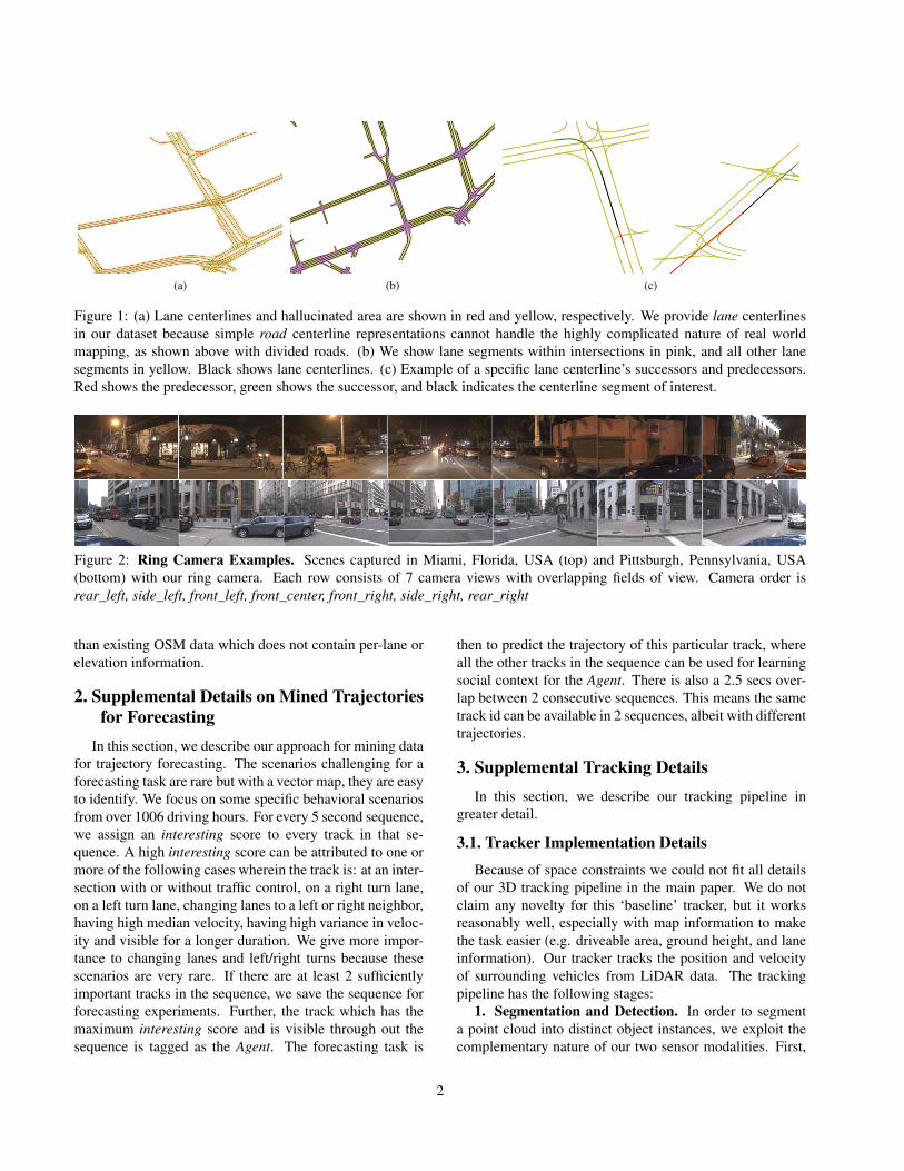
Figure 2: Ring Camera Examples. Scenes captured in Miami, Florida, USA (top) and Pittsburgh, Pennsylvania, USA(bottom) with our ring camera. Each row consists of 7 camera views with overlapping fields of view. Camera order isrear_left, side_left, front_left, front_center, front_right, side_right, rear_right

than existing OSM data which does not contain per-lane orelevation information.

2. Supplemental Details on Mined Trajectoriesfor Forecasting

In this section, we describe our approach for mining datafor trajectory forecasting. The scenarios challenging for aforecasting task are rare but with a vector map, they are easyto identify. We focus on some specific behavioral scenariosfrom over 1006 driving hours. For every 5 second sequence,we assign an interesting score to every track in that se-quence. A high interesting score can be attributed to one ormore of the following cases wherein the track is: at an inter-section with or without traffic control, on a right turn lane,on a left turn lane, changing lanes to a left or right neighbor,having high median velocity, having high variance in veloc-ity and visible for a longer duration. We give more impor-tance to changing lanes and left/right turns because thesescenarios are very rare. If there are at least 2 sufficientlyimportant tracks in the sequence, we save the sequence forforecasting experiments. Further, the track which has themaximum interesting score and is visible through out thesequence is tagged as the Agent. The forecasting task is

then to predict the trajectory of this particular track, whereall the other tracks in the sequence can be used for learningsocial context for the Agent. There is also a 2.5 secs over-lap between 2 consecutive sequences. This means the sametrack id can be available in 2 sequences, albeit with differenttrajectories.

3. Supplemental Tracking DetailsIn this section, we describe our tracking pipeline in

greater detail.

3.1. Tracker Implementation Details

Because of space constraints we could not fit all detailsof our 3D tracking pipeline in the main paper. We do notclaim any novelty for this ‘baseline’ tracker, but it worksreasonably well, especially with map information to makethe task easier (e.g. driveable area, ground height, and laneinformation). Our tracker tracks the position and velocityof surrounding vehicles from LiDAR data. The trackingpipeline has the following stages:

1. Segmentation and Detection. In order to segmenta point cloud into distinct object instances, we exploit thecomplementary nature of our two sensor modalities. First,

2

Function name Description

remove_non_driveable_area_points Use rasterized driveable area ROI to decimate LiDAR point cloud toonly ROI points.

remove_ground_surface Remove all 3D points within 30 cm of the ground surface.get_ground_height_at_xy Get ground height at provided (x,y) coordinates.render_local_map_bev_cv2 Render a Bird’s Eye View (BEV) in OpenCV.render_local_map_bev_mpl Render a Bird’s Eye View (BEV) in Matplotlib.get_nearest_centerline Retrieve nearest lane centerline polyline.get_lane_direction Retrieve most probable tangent vector ∈ R2 to lane centerline.get_semantic_label_of_lane Provide boolean values regarding the lane segment, including is_intersection

turn_direction, and has_traffic_control.get_lane_ids_in_xy_bbox Get all lane IDs within a Manhattan distance search radius in the xy plane.get_lane_segment_predecessor_ids Retrieve all lane IDs with an incoming edge into the query lane segment in the

semantic graph.get_lane_segment_successor_ids Retrieve all lane IDs with an outgoing edge from the query lane segment.get_lane_segment_adjacent_ids Retrieve all lane segment IDs of that serve as left/right neighbors to the query

lane segment.get_lane_segment_centerline Retrieve polyline coordinates of query lane segment ID.get_lane_segment_polygon Hallucinate a lane polygon based around a centerline using avg. lane width.get_lane_segments_containing_xy Use a “point-in-polygon” test to find lane IDs whose hallucinated lane polygons

contain this (x, y) query point.

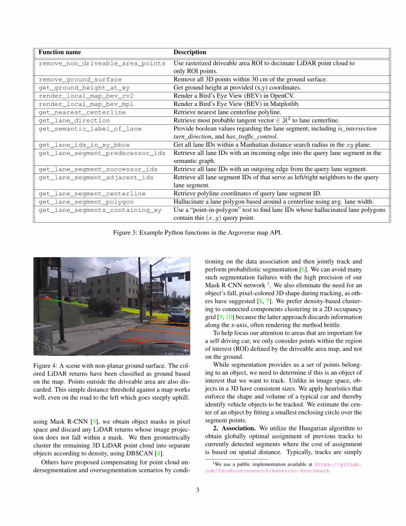
Figure 3: Example Python functions in the Argoverse map API.

Figure 4: A scene with non-planar ground surface. The col-ored LiDAR returns have been classified as ground basedon the map. Points outside the driveable area are also dis-carded. This simple distance threshold against a map workswell, even on the road to the left which goes steeply uphill.

using Mask R-CNN [5], we obtain object masks in pixelspace and discard any LiDAR returns whose image projec-tion does not fall within a mask. We then geometricallycluster the remaining 3D LiDAR point cloud into separateobjects according to density, using DBSCAN [4].

Others have proposed compensating for point cloud un-dersegmentation and oversegmentation scenarios by condi-

tioning on the data association and then jointly track andperform probabilistic segmentation [6]. We can avoid manysuch segmentation failures with the high precision of ourMask R-CNN network 1. We also eliminate the need for anobject’s full, pixel-colored 3D shape during tracking, as oth-ers have suggested [8, 7]. We prefer density-based cluster-ing to connected components clustering in a 2D occupancygrid [9, 10] because the latter approach discards informationalong the z-axis, often rendering the method brittle.

To help focus our attention to areas that are important fora self driving car, we only consider points within the regionof interest (ROI) defined by the driveable area map, and noton the ground.

While segmentation provides us a set of points belong-ing to an object, we need to determine if this is an object ofinterest that we want to track. Unlike in image space, ob-jects in a 3D have consistent sizes. We apply heuristics thatenforce the shape and volume of a typical car and therebyidentify vehicle objects to be tracked. We estimate the cen-ter of an object by fitting a smallest enclosing circle over thesegment points.

2. Association. We utilize the Hungarian algorithm toobtain globally optimal assignment of previous tracks tocurrently detected segments where the cost of assignmentis based on spatial distance. Typically, tracks are simply

1We use a public implementation available at https://github.com/facebookresearch/maskrcnn-benchmark.

3

assigned to their nearest neighbor in the next frame.3. Tracking. We use ICP (Iterative Closest Point) from

the Point Cloud Library [12] to estimate relative transforma-tion between corresponding point segments for each track.Then we apply a Kalman Filter (KF) [7] with ICP resultsas the measurement and a static motion model (or constantvelocity motion model, depending on the environment) toestimate vehicle poses for each tracked vehicle. We assigna fixed size bounding box for each tracked object. The KFstate is comprised of both the 6 dof pose and velocity.

3.2. Tracking Evaluation Metrics

We use standard evaluation metrics commonly used formultiple object trackers (MOT) [11, 1]. The MOT metricrelies on centroid distance as distance measure.

• MOTA(Multi-Object Tracking Accuracy):

MOTA = 100∗ (1−∑

t FNt + FPt + IDsw∑t GT

) (1)

where FNt, FPt, IDsw, GT denote number of falsenegative, false positives, number of ID switches, andground truths. We report MOTA as percentages.

• MOTP(Multi-Object Tracking Precision):

MOTP =

∑i,t D

it∑

t Ct(2)

where Ct denotes the number of matches, and Dit de-

notes the distance of matches.

• IDF1 (F1 score):

IDF1 = 2precision ∗ recallprecision+ recall

(3)

Where recall is the number of true positives over num-ber of total ground truth labels. precision is the num-ber of true positives over sum of true positives andfalse positives.

• MT (Mostly Tracked): the ratio of trajectories trackedmore than 80% of its lifetime.

• ML (Mostly Lost): the ratio of trajectories trackedless than 20% of its lifetime.

• FP (False Positive): Total number of false positives

• FN (False Negative): Total number of false negatives

• IDsw (ID Switch): number of identified ID switches

• Frag (Fragmentation): Total number of switchesfrom "tracked" to "not tracked"

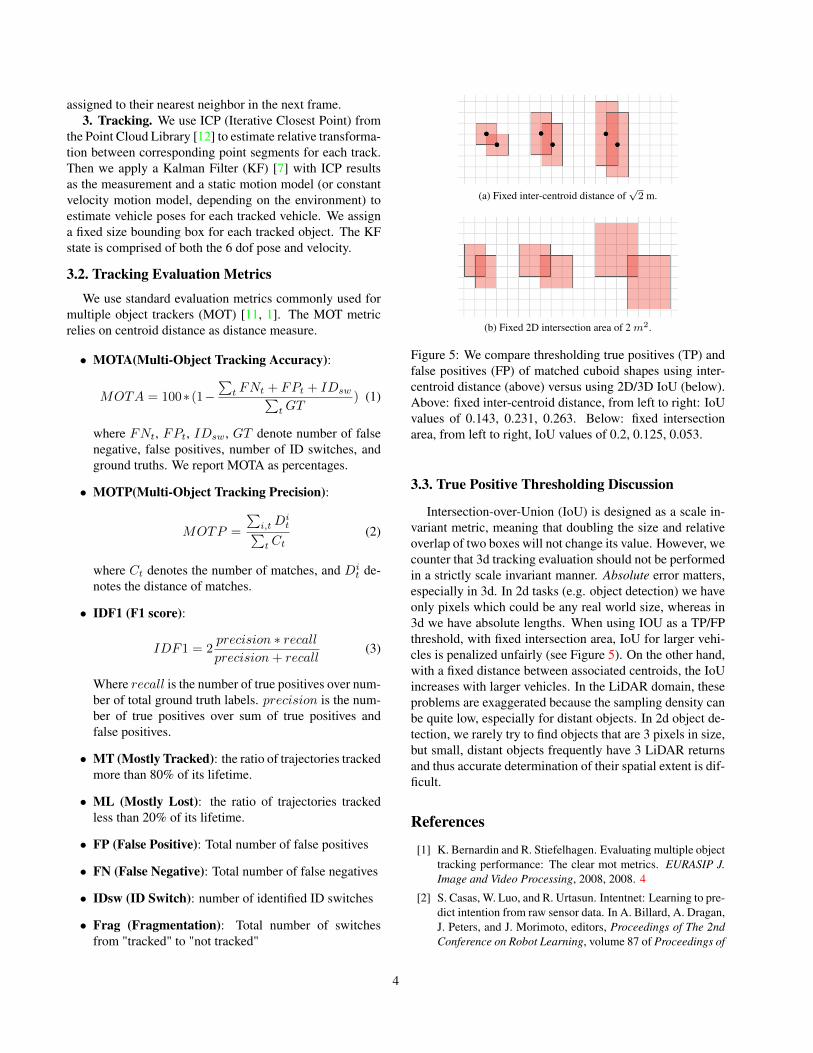
(a) Fixed inter-centroid distance of√2 m.

(b) Fixed 2D intersection area of 2 m2.

Figure 5: We compare thresholding true positives (TP) andfalse positives (FP) of matched cuboid shapes using inter-centroid distance (above) versus using 2D/3D IoU (below).Above: fixed inter-centroid distance, from left to right: IoUvalues of 0.143, 0.231, 0.263. Below: fixed intersectionarea, from left to right, IoU values of 0.2, 0.125, 0.053.

3.3. True Positive Thresholding Discussion

Intersection-over-Union (IoU) is designed as a scale in-variant metric, meaning that doubling the size and relativeoverlap of two boxes will not change its value. However, wecounter that 3d tracking evaluation should not be performedin a strictly scale invariant manner. Absolute error matters,especially in 3d. In 2d tasks (e.g. object detection) we haveonly pixels which could be any real world size, whereas in3d we have absolute lengths. When using IOU as a TP/FPthreshold, with fixed intersection area, IoU for larger vehi-cles is penalized unfairly (see Figure 5). On the other hand,with a fixed distance between associated centroids, the IoUincreases with larger vehicles. In the LiDAR domain, theseproblems are exaggerated because the sampling density canbe quite low, especially for distant objects. In 2d object de-tection, we rarely try to find objects that are 3 pixels in size,but small, distant objects frequently have 3 LiDAR returnsand thus accurate determination of their spatial extent is dif-ficult.

References

[1] K. Bernardin and R. Stiefelhagen. Evaluating multiple objecttracking performance: The clear mot metrics. EURASIP J.Image and Video Processing, 2008, 2008. 4

[2] S. Casas, W. Luo, and R. Urtasun. Intentnet: Learning to pre-dict intention from raw sensor data. In A. Billard, A. Dragan,J. Peters, and J. Morimoto, editors, Proceedings of The 2ndConference on Robot Learning, volume 87 of Proceedings of

4

(a) Argoverse LiDAR (b) Argoverse LiDAR

(c) KITTI LiDAR (d) nuScenes LiDAR

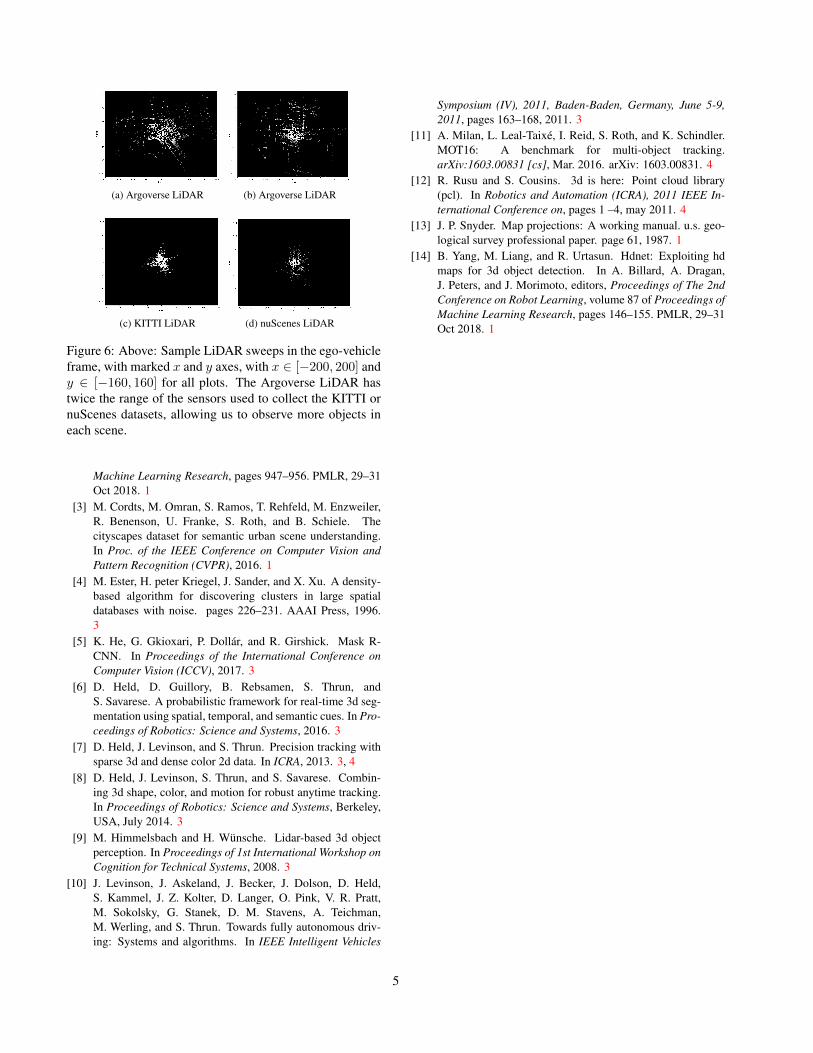
Figure 6: Above: Sample LiDAR sweeps in the ego-vehicleframe, with marked x and y axes, with x ∈ [−200, 200] andy ∈ [−160, 160] for all plots. The Argoverse LiDAR hastwice the range of the sensors used to collect the KITTI ornuScenes datasets, allowing us to observe more objects ineach scene.

Machine Learning Research, pages 947–956. PMLR, 29–31Oct 2018. 1

[3] M. Cordts, M. Omran, S. Ramos, T. Rehfeld, M. Enzweiler,R. Benenson, U. Franke, S. Roth, and B. Schiele. Thecityscapes dataset for semantic urban scene understanding.In Proc. of the IEEE Conference on Computer Vision andPattern Recognition (CVPR), 2016. 1

[4] M. Ester, H. peter Kriegel, J. Sander, and X. Xu. A density-based algorithm for discovering clusters in large spatialdatabases with noise. pages 226–231. AAAI Press, 1996.3

[5] K. He, G. Gkioxari, P. Dollár, and R. Girshick. Mask R-CNN. In Proceedings of the International Conference onComputer Vision (ICCV), 2017. 3

[6] D. Held, D. Guillory, B. Rebsamen, S. Thrun, andS. Savarese. A probabilistic framework for real-time 3d seg-mentation using spatial, temporal, and semantic cues. In Pro-ceedings of Robotics: Science and Systems, 2016. 3

[7] D. Held, J. Levinson, and S. Thrun. Precision tracking withsparse 3d and dense color 2d data. In ICRA, 2013. 3, 4

[8] D. Held, J. Levinson, S. Thrun, and S. Savarese. Combin-ing 3d shape, color, and motion for robust anytime tracking.In Proceedings of Robotics: Science and Systems, Berkeley,USA, July 2014. 3

[9] M. Himmelsbach and H. Wünsche. Lidar-based 3d objectperception. In Proceedings of 1st International Workshop onCognition for Technical Systems, 2008. 3

[10] J. Levinson, J. Askeland, J. Becker, J. Dolson, D. Held,S. Kammel, J. Z. Kolter, D. Langer, O. Pink, V. R. Pratt,M. Sokolsky, G. Stanek, D. M. Stavens, A. Teichman,M. Werling, and S. Thrun. Towards fully autonomous driv-ing: Systems and algorithms. In IEEE Intelligent Vehicles

Symposium (IV), 2011, Baden-Baden, Germany, June 5-9,2011, pages 163–168, 2011. 3

[11] A. Milan, L. Leal-Taixé, I. Reid, S. Roth, and K. Schindler.MOT16: A benchmark for multi-object tracking.arXiv:1603.00831 [cs], Mar. 2016. arXiv: 1603.00831. 4

[12] R. Rusu and S. Cousins. 3d is here: Point cloud library(pcl). In Robotics and Automation (ICRA), 2011 IEEE In-ternational Conference on, pages 1 –4, may 2011. 4

[13] J. P. Snyder. Map projections: A working manual. u.s. geo-logical survey professional paper. page 61, 1987. 1

[14] B. Yang, M. Liang, and R. Urtasun. Hdnet: Exploiting hdmaps for 3d object detection. In A. Billard, A. Dragan,J. Peters, and J. Morimoto, editors, Proceedings of The 2ndConference on Robot Learning, volume 87 of Proceedings ofMachine Learning Research, pages 146–155. PMLR, 29–31Oct 2018. 1

5