Embed Size (px)
Citation preview
The author(s) shown below used Federal funds provided by the U.S.Department of Justice and prepared the following final report:
Document Title: Crime Hot Spot Forecasting: Modeling andComparative Evaluation, Summary
Author(s): Wilpen Gorr ; Andreas Olligschlaeger
Document No.: 195168
Date Received: July 03, 2002
Award Number: 98-IJ-CX-K005
This report has not been published by the U.S. Department of Justice.To provide better customer service, NCJRS has made this Federally-funded grant final report available electronically in addition totraditional paper copies.
Opinions or points of view expressed are thoseof the author(s) and do not necessarily reflect
the official position or policies of the U.S.Department of Justice.
Summary
Crime Hot Spot Forecasting: Modeling and Comparative Evaluation
Grant 98-W-CX-KO05
Wilpen Gorr
and
Andreas Olligschlaeger
May 6,2002 PROPERTY OF
National Criminal Justice Reference Service (NCJRS) Box 6000 Rcckville, MD 20849-6000
.
and do not necessarily reflect the official position or policies of the U.S. Department of Justice. been published by the Department. Opinions or points of view expressed are those of the author(s) This document is a research report submitted to the U.S. Department of Justice. This report has not
1
Crime mapping is a critical tool for use in crime prevention and law enforcement.
Electronic computer maps displaying data from police record management systems,
computer aided dispatch, and other sources have directed attention to the criminality of
places and led to new approaches to policing including hot spot enforcement, Compstat,
and geographic profiling.’
Often key to success in crime mapping are crime data and maps that are up to date, with
the latest events and patterns available for analysis and use. Crime maps portray valuable
information to the extent that criminals are creatures of habit, repeatedly using the same
locales for committing crimes, or are attracted to certain high crime risk areas. There are
situations, however, in which crime patterns change over time. For example,
enforcement may cause crime to displace in location, the arrival of college students to an
urban campus in late August may lead to an increase in robberies near and on campus
because of the availability of good targets for criminals, and a rivalry between
neighboring gangs may reach the boiling point causing a gang war and violent crimes.
These are situations in which it would be desirable to forecast crime.
Many police resources are mobile and easily transferred to or focused on different
locations immediately. Consequently, short-term, one-month-ahead forecasts are
sufficient for many law enforcement and crime prevention purposes. Fortunately such
forecasting methods are among the most-studied because of their many business
applications. The most common short-term forecasting approach is to extrapolate or
extend established time-based patterns including time trend (steady increase of decrease
of crime level with advancing time) and seasonal adjustments into the future. For
example, if robberies have a trend decreasing on average four per month but next month
is July, a peak month on average having a seasonal increase of 10 robberies, the forecast
for July would include a net change over June of plus six robberies. Such an
extrapolation constitutes a “business as usual” forecast, merely continuing the established
time patterns with no “surprises.” Besides often yielding the most accurate short-term
forecasts, extrapolations also make a good basis of comparison, “counterfactual cases”, e
and do not necessarily reflect the official position or policies of the U.S. Department of Justice. been published by the Department. Opinions or points of view expressed are those of the author(s) This document is a research report submitted to the U.S. Department of Justice. This report has not

2
for evaluating enforcement activities because of their business-as-usual nature. One
compares the extrapolative (counterfactual) forecast with the actual crime level of the
same month. If the actual crime level is much different than the forecast, then there is
evidence of a change in crime patterns. Note that extrapolative methods are also called
“univariate methods” because they include only one substantive variable, which for crime
forecasting would generally be crime counts, and a time index (e.g., month serial number
e
/
with the oldest month having the index 1). I
A more sophisticated approach to short-term forecasting uses leading indicators, if they
can be shown to exist and are available. For example, a sharp increase in certain minor
crimes and disturbances in an area this month may indicate the presence and building of a
criminal element and therefore forecast an increase in serious crimes next month. The
minor crimes and disturbances are the leading indicators. Enforcement and spatial crime
displacement may yield another leading indicator. For example, a crackdown on drugs at
a hot spot this month may lead to drug dealing in a nearby area next month. In this case,
drug offenses in a locale is a leading indicator. These sorts of changes in crime patterns
do not fall into the “business-as-usual category,” but are unforeseeable as simple
extrapolations.
Leading indicator forecasting, such as done in macroeconomic and other advanced
forecasting problems, requires multivariate statistical modeling; for example, multiple
regression models. We build and test regression models for crime forecasting. A
comprehensive crime forecasting system would include both extrapolative and leading
indicator forecasting. Most forecasts used in practice would be extrapolative, but in the
background, leading indicator models would be looking for big, otherwise unexpected
changes.
The research reported in this summary is among the earliest attempts to determine the
feasibility of crime forecasting, including both extrapolative methods and leading a
and do not necessarily reflect the official position or policies of the U.S. Department of Justice. been published by the Department. Opinions or points of view expressed are those of the author(s) This document is a research report submitted to the U.S. Department of Justice. This report has not
3
indicator models. We compare common police practices with simple, widely-used
forecast models through a state-of-art experimental design and extensive police data from
Pittsburgh, Pennsylvania. While initial results are promising, we do not know if crime
forecasting will ultimately be accurate enough for use by police. Nevertheless, to give a
concrete idea of how crime forecasting could fit into policing and crime mapping, we
next provide a use case scenario - a fictional story. It is the target that we envision for
research on crime forecasting. After providing the scenario, we proceed to review .the I alternative approaches to short-term forecasting in more depth, and then describe our
Pittsburgh case study for evaluating forecasts. Following those sections is a description
of our experimental design for assessing forecast accuracy, which is followed by results.
Last are recommendations for practitioners and researchers, including areas for future
research.
Use Case Scenario
Suppose that it is June 3,2005. Precinct 2 of the Pittsburgh Police Bureau is on deck at
the monthly planning and review (Compstat) meeting. The precinct 2 commander starts
by saying, “Let’s take a look first, at what happened last month with part 1 violent
crimes.” On a projected computer screen is a grid map covering all of Pittsburgh,
showing forecasted changes in part 1 violent crimes from April to May 2005. Areas that
were forecasted to have increases in violent crimes are shown in shades of red (the darker
the shade, the larger the increase) and areas forecasted to have decreases are in shades of
blue
The commander of Precinct 2 continues: “The five dark red grid cells with arrows
pointing to them were the ones forecasted in April to have large crime increases in May.
In all five grid cells, leading indicators including simple assaults, shots fired calls, and
criminal mischief all spiked up in April, making the high violent crime forecasts that we
had for May. We carried out a number of special actions tailored for each identified grid a
and do not necessarily reflect the official position or policies of the U.S. Department of Justice. been published by the Department. Opinions or points of view expressed are those of the author(s) This document is a research report submitted to the U.S. Department of Justice. This report has not
cell, after studying the zoomed-in pin maps and crime reports for the April leading
indicators and violent crimes.”
“The result was seven major arrests and only one of the grid cells actually flared up, as
you can see in this next map.” The next map has actual violent crime changes from April
to May 2005, with the same five grid cells identified. Two of the grid cells had no
significant changes, two cooled off, and only one had the forecasted increase. One of the
no-change cells and one of the cooled-off cells look like they were duds. There were no
significant arrests or other signs of the forecasted flare ups there. The commander
continues: “Regardless, we think that we were able to nip most of last month’s new
violent crime problems in the bud. We’ll pull our special squads out of the four grid cells
that didn’t flare up and redeploy them to new flare ups forecasted for June. All four grid
cells that we’re pulling out of are forecasted to stay low in June, but we’ll keep an eye on
their CAD calls and crime reports.”
“Let’s turn now, to the forecasts for next month. The next map is a forecasted change
map for June. In part, we expect increases in violent crimes due to seasonal effects, as
summer gets going. This map shows six grid cells heating up, with leading indicators in
May spiking up, especially shots fired, simple assaults, and CAD drug calls. The drug
markets are heating up. Let’s take a look at the first grid cell, would you please zoom
into grid cell 87? OK, you can see that drug calls and shots fired are up in the
southeastern block of that grid cell, that’s the Kelly Street drug market. We’re going to
move on undercover work, make arrests, and we’re going to maintain a police presence
around the clock in that area of the grid cell.” The presentation and mapping displays
continue through the rest of the forecasted flare-up grid cells. This ends the use case
scenario.
and do not necessarily reflect the official position or policies of the U.S. Department of Justice. been published by the Department. Opinions or points of view expressed are those of the author(s) This document is a research report submitted to the U.S. Department of Justice. This report has not

5
Approaches to Short-Term Forecasting
There has been a great deal of applied research in the field of forecastin over the last
twenty-five years with many advances, especially with short-term forecasting methods
and experimental designs for their evaluation. As this literature suggests, our strategy for
assessing short-term crime forecasting is to use well-established, simple methods first and
then proceed to more advanced methods later as merited.
I 1
A unique feature of crime forecasting, in contrast to the great body of the forecasting
literature, is that it involves time and space series data; for example, monthly crime
counts for all uniform grid cells covering a jurisdiction. Most forecast methods were
developed for single time series. One opportunity with time and space series data over
traditional time series is the ability to create new variables, based on data from
neighboring grid cells, that can estimate the effects of crime spillover, displacement, and
other spatial interactions? The biggest challenge of forecasting space and time series
data is to accurately forecast crime counts in as small grid cells (or other area units) as
possible. Our research thus far has shown that grid cells need to be quite a bit larger than
individual hot spots areas, about ten blocks on a side. Crime forecasting is nevertheless
valuable at this scale, drawing attention to areas needing further study through pin
mapping such as the Kelly Street drug market example in the use case scenario. The
smallest administrative areas of interest to police is car beats (or patrol districts) and these
are approximately twice as large as 4,000 foot grid cells on the average in Pittsburgh, and
approximately the same size in densely populated areas.
The fundamental result of the more recent empirical research on forecasting is that
alternative forecast methods should be compared based on forecast accuracy and simple
methods should be used unless more complicated ones prove to be more accurate. While
seemingly obvious, this was not the accepted approach in the 1970s and 1980s. It used to
be that the most theoretically appealing and rigorous methods were favored, but in
and do not necessarily reflect the official position or policies of the U.S. Department of Justice. been published by the Department. Opinions or points of view expressed are those of the author(s) This document is a research report submitted to the U.S. Department of Justice. This report has not
general, empirical research has shown that such methods have not improved forecast
acc~racy .~ We follow this pragmatic result and compare three kinds of simple forecast
approaches based on forecast accuracy through experimentation: data methods that are
not model-based (the random walk and a related common police practice), exponential
smoothing univariate methods, and multiple regression leading indicator models. For the
univariate methods, we use multiplicative Classical Decomposition to remove seasonality
from the time series data and add it back into forecasts. We explain each of these .
methods in general terms next. Note that it is not the purpose of this summary to describe
these methods in computational detail. They can be found in many standard textbooks
and are implemented in many software programs4. Our current research is producing
prototype forecasting software and will include detailed descriptions for implementation.
The so-called random walk (or ndive) method takes the most recent month’s actual crime
count as next month’s forecast. This is a competitive method in contexts for time series
data that undergo frequent time pattern changes, including step jumps and turning points,
but do not have strong time trends and seasonality. The random walk is memory less - it
just uses the last data point - and thus adjusts immediately to pattern changes, while most
other methods retain the influence of past data (i.e., have memories). Of course the
random walk cannot forecast step jumps or other pattern changes, but merely adjusts to
them immediately after they occur. If there are time trends or seasonality, the random
walk has no ability to forecast such patterns and thus does poorly. Also, if data are very
noisy (with frequent large changes up and down but no time pattern changes), the random
walk has no benefit of averaging and thus is unreliable as a forecaster - this seems to be
the case for crime forecasting.
0
The most common data-based, non-model police method uses a month’s data point from
a year ago as the forecast of the same month this year. For monthly data, we call this
method “naTve lag 12.” For example, in May 2005 the forecast made for June 2005 is the
data point from June 2004. This method, commonly used as the comparison point (i.e.,
counterfactual) for judging performance in Compstat meetings5. It also has the advantage a
and do not necessarily reflect the official position or policies of the U.S. Department of Justice. been published by the Department. Opinions or points of view expressed are those of the author(s) This document is a research report submitted to the U.S. Department of Justice. This report has not
7
of accounting for seasonality; for example, one uses an old June data point to forecast a
new June, and thus one observation of June seasonality is included. The problems with
this method, however, are many. It includes all of the problems of the random walk, plus
ignores an entire year of trend and pattern changes. It also destroys the comparative
advantage of the random walk’s ability to immediately adjust to pattern changes, because
the data point used as the forecast is a year old. As we shall see, this is the very worst
forecast and comparison method if one is attempting to assess police activities.
Ndive and nahe lag 12 are examples of the more general univariate forecast methods.
The two most common univariate model components are: time trend (most often linear,
estimating a steady increase or decrease in crime counts with each increase in the time
index) and seasonality (additive or multiplicative adjustment to the linear time trend for
each month). An additive seasonal adjustment add or subtracts a number of crimes for
each month; for example, add 10 for July, subtract 6 for February. A multiplicative
seasonal adjustment is a unit less factor for each month; for example multiply the linear
time trend by 1.25 for July and by 0.80 for February. For time and space series data, we
need to use multiplicative seasonality factors because they scale themselves for use in
both high crime and low crime areas. In contrast, additive seasonal adjustments would
have to be separately estimated for high versus low crime areas.
A third type of univariate model component is autoregressive/moving averages.
Autoregressive/moving averages correct for forecast errors; for example, if there are
several errors of the same sign in time sequence (e.g., most recent forecasts are too low),
it is likely that the next forecast will have the same error (too low) and this information
can be included in the forecast as an adjustment. These methods; however, are complex
to use and have had only limited success in improving forecast accuracy. Hence, we do
not use them in our research at this time. Simpler univariate methods, such as the ones
that we use - exponential smoothing for linear time trend estimation and classical
decomposition for multiplicative seasonality - have been consistently among the most
accurate forecasters for a wide variety of data in the short-term. There are more complex e
and do not necessarily reflect the official position or policies of the U.S. Department of Justice. been published by the Department. Opinions or points of view expressed are those of the author(s) This document is a research report submitted to the U.S. Department of Justice. This report has not
8
and often somewhat superior univariate methods, but they should be investigated later
after we learn from the simpler methods.
Exponential smoothing methods are based on weighted averages. For estimating the time
trend of monthly crime counts, exponential smoothing methods place the most weight on
the most recent month’s data point. Weights on older data points get smaller quickly
(reduce exponentially) with the age of the data. The result is a time trend that bestfits the
most recent data, and that can self-adapt to changes in time trends, albeit with a time lag.
We used two variations of exponential smoothing: simple exponential smoothing and
Holt linear trend exponential smoothing. The former estimates the average of a time
series and uses the last estimated month as the forecast for next month. The latter also
includes a time trend component and thus the forecast is the average for the most recent
month plus a time trend change. Note that the analyst must estimate a separate univariate
model for each area unit (grid cell, car beat, etc.), presumably with automated software.
A benefit is that each area gets its own, custom model. The flip-side difficulty is that
each area needs to have a sufficiently high crime volume to allow reliable estimation of
models - this is the central problem in applying univariate methods to crime forecasting.
I
We used Classical Decomposition, a widely-used simple method, to estimate
multiplicative seasonal factors. This method uses a moving average approach to estimate
seasonal factors. The moving average is 13 months long, centered on the month of
interest, say July of a given year. The ratio of the July data point divided by the centered
average is an observation of the multiplicative July seasonal impact. Such data points,
computed for all July observations in the full estimation data set, are averaged to yield the
July seasonal factor. A rule of thumb suggests that monthly time series be at least five
years long to permit adequate estimation of seasonal factors.
Leading indicator forecast models are multivariate, relating current values of the
dependent variable to past values of independent variables. Current crime theories
and do not necessarily reflect the official position or policies of the U.S. Department of Justice. been published by the Department. Opinions or points of view expressed are those of the author(s) This document is a research report submitted to the U.S. Department of Justice. This report has not

9
suggest the existence of crime leading indicators; for example, “broken windows” and
routine activities.6 We find that counts of simple assaults, shots fired calls, criminal
mischief, drug calls, disorderly conduct offenses, and other part 2 offenses and CAD calls
in a given month forecast counts of part 1 violent crimes in the next month. Successful
leading indicators can forecast what otherwise would be surprises - departures from past
patterns that one cannot foresee with univariate forecasts. If a leading indicator
undergoes a large step jump or trend reversal, then the corresponding forecast can also
make the same break from a historical pattern. Note that generally an analyst would
estimate a single leading indicator model covering all geographic areas, in contrast with
the case of a separate model per area of univariate methods.
Leading indicators are potentially successful, and more accurate than univariate methods
in limited circumstances; namely, if
Leading indicators are available with the same data frequency as the dependent
variable (e.g., as monthly data) and are strongly predictive of the dependent
variable.
The estimated multiple regression or other model is stable over time and space,
with accurately estimated coefficients for leading indicators.
The leading indicators undergo occasional large changes, yielding to forecasts
that are more accurate than univariate extrapolations under those conditions.
Selected part 2 crimes and computer aided dispatch (CAD) calls are promising leading
indicators for part 1 violent and property crimes and CAD drug calls. Expectations need
to be somewhat guarded; however, for leading indicator crime forecasting because of the
high complexity of the phenomena and the very small areas under study and at which our
needs lie. On the positive side, we have only attempted the simplest models in the
current research and there are clear approaches to improving these models.
and do not necessarily reflect the official position or policies of the U.S. Department of Justice. been published by the Department. Opinions or points of view expressed are those of the author(s) This document is a research report submitted to the U.S. Department of Justice. This report has not
10
Case Study
Pittsburgh, Pennsylvania, our study area, is a medium-size city of approximately 370,000
population and 55 square miles. It has six precincts and 46 car beats. We collected all
offense reports and 91 1 CAD calls in electronic form from the Pittsburgh Bureau of
Police for 1990 through 1998. Our data processing included address matching to place
the data in a GIs, spatial overlay to geocode crime points with area unit identifiers (grid
cells, precincts, etc.), specification and aggregation of crime types to leading indicators
and dependent variables, creation of time and spatial lags of leading indicators, and
aggregation to produce monthly, grid cell or other areal unit series for selected crimes.
The spatial lags are leading indicators averaged over all neighboring cells that touch a
data observation cell (along a line or at a point).
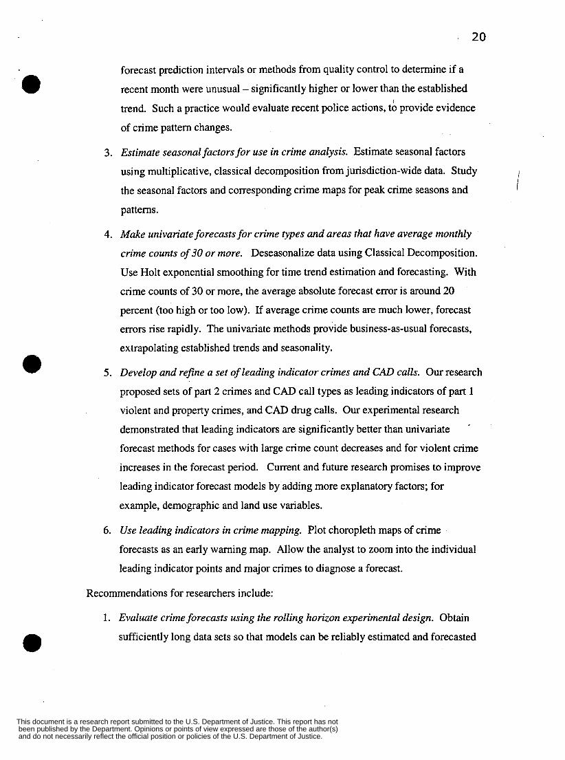
Exhibit 1 displays monthly time series plots for part 1 violent crimes (with robbery
included), part 1 property crimes (with robbery also included), and CAD drug calls7.
These plots cover the entire period of data used from 1990 through 1998 and for all of
Pittsburgh. We standardized the scale of each time series to facilitate comparisons (we
adjusted the mean of each time series to be zero and standard deviation to be one, a
common practice for comparing data). Data from 1990 through the end of 1995 served as
estimation data to estimate model coefficients. Then data from January 1996 through
December 1998 were forecasted one month ahead, using a rolling horizon design to be
described later.
Time pattern changes in these data contribute to the challenge of forecasting them
accurately. From 1990 through 1992, crime had an increasing time trend. Then from
1993 through about 1995, crimes decreased strongly. Thus the estimation period had two
major time patterns, and the older pattern needed to be “forgotten” by methods. Next, in
our hold-out sample period starting in 1996, crimes flattened out and reversed time trend,
and started to gradually increase again through 1998. Thus forecast models had to e
and do not necessarily reflect the official position or policies of the U.S. Department of Justice. been published by the Department. Opinions or points of view expressed are those of the author(s) This document is a research report submitted to the U.S. Department of Justice. This report has not

11
accommodate turning points and trend reversals as we entered forecast periods. Note that
individual precincts and grid cells generally followed the total Pittsburgh pattern, but
significant sub-trends and other variations existed. For example, during 1996-1998,
many sub-areas stayed flat over time while others increased sharply. We conclude that
this real-world case study has some real challenges for forecasting.
While we forecasted data for many different kinds of area units, including precincts, car
beats, and census tracts, we decided to restrict our research to precincts and, primarily,
uniform square grid cells. Data displayed as color coding in grid cells are easiest to
comprehend on maps. The eye easily integrates information from individual cells, seeing
patterns immediately, because two visual variables are eliminated (size and shape of area
unit). Crime maps can display precincts and car beat boundaries superimposed over
color-coded grid cells, to easily relate grid cell patterns to administrative areas.
Furthermore, the user of a desktop or Web GIS can zoom-in to see underlying pin maps
and thus obtain the finest detail of spatial information. Color-coded change maps based
on grid cells, such as the ones described in the use case scenario, form the basis of early
warning forecast systems, providing jurisdiction-wide scanning. Users then can zoom
into grid cells of interest (e.g., dark red cells) for pin map details.
We eventually settled on a 4,000 foot grid cell as the smallest practical for forecasting in
Pittsburgh, working our way up from smaller grid cell sizes starting at 1,500 feet. The
smaller grid cells led to data aggregates that were too small for reliable model estimation,
a point that we will discuss at length below. Exhibit 2 displays July 1991 robbery and
CAD drug call points with a background of Pittsburgh boundaries, its three major rivers,
and the 4,000 foot grid. The two crimes chosen for display here are among the most
clustered, and here we can see that the grid cells are fairly good at capturing clusters of
one or few hot spot areas. While not as small as hoped, we are reasonably pleased with
the representation provided by the 4,000 foot grid system.
and do not necessarily reflect the official position or policies of the U.S. Department of Justice. been published by the Department. Opinions or points of view expressed are those of the author(s) This document is a research report submitted to the U.S. Department of Justice. This report has not

12
Experimental Design
We conducted forecast experiments, comparing forecast accuracy of several forecast
methods. We made forecasts with no knowledge of any future values, including the
crime counts that we were forecasting nor independent variables used in multivariate
models. The latter were all leading indicators, with known values at the time forecasts
were made, as would be the case in practice.
We used the rolling-horizon experimental design, which maximizes the number of
forecasts for a given time series at different times and under different conditions. In this
design, we use several forecast models and make alternative forecasts in parallel. For
each forecast model included in an experiment, we estimate models on training data,
forecast one month ahead to new data not previously seen by the model, and calculate
and save the forecast error. Then we roll forward one month, adding the observed value
of the previously forecasted data point to the training data, dropping the oldest historical
data point, and forecasting ahead to the next month. We made forecasts over a 36 month
period (January 1996 through December 1998), in order to generate an adequate sample
size of forecast errors for statistical testing purposes. This provided 36 forecast errors per
univariate method and area, and 5,076 (36 months x 141 grid cells) per multivariate
model.
0
We conducted two experimental studies. Study 1 had the purpose of determining the best
univariate forecast method for one-month-ahead crime forecasts. This study included:
A representative set of individual crime types to forecast: simple assault,
aggravated assault, robbery, burglary, and CAD drug calls. These include part
1 property and violent crimes, a part 2 crime, and a CAD call variable. Some
are high frequency crimes (simple assaults and burglaries), others are low
frequency (aggravated assault and robbery).
and do not necessarily reflect the official position or policies of the U.S. Department of Justice. been published by the Department. Opinions or points of view expressed are those of the author(s) This document is a research report submitted to the U.S. Department of Justice. This report has not
13
0 The six precincts in Pittsburgh as the area units. This proved to be a good
choice, because there still remained a large variation in crime counts per areal
unit, from quite small to large. This is the most critical variable in determining
forecast accuracy, as will be shown below.
Random Walk (nayve method), narve Lag 12 (police method), simple exponential
smoothing, Holt linear trend exponential smoothing - all with and without
deseasonalized data. Smoothing methods had smoothing parameters optifnized
in usual ways'. We used seasonal estimates made individually by precinct and
made from all of Pittsburgh for pooled estimates. The tradeoff confronted by the
two approaches for seasonal estimation is more reliable estimates from pooling
versus tailored seasonal factors for different kinds of areas (commercial,
residential, etc.).
Rolling five years of estimation data and three years of one-month-ahead
forecasts.
The best univariate forecast method from study 1 is Holt exponential smoothing with
pooled estimates of seasonality, but more follows on this in the results section. Study 2
pits this univariate method against leading indicator models. Features of the second
study include:
Three dependent variables -part I violent crimes (aggravated assaults, robbery,
rape, and homicide), part I property crimes (burglary, larceny, motor vehicle
theft, arson, and robbery), and CAD drug calls. We aggregated crimes up to
larger collections in part to increase crime counts per grid cell. We maintained
violent versus property crime categories because the two types of crime have
different behaviors and leading indicators. Drug calls were included because of
their importance in causing so many other crimes.
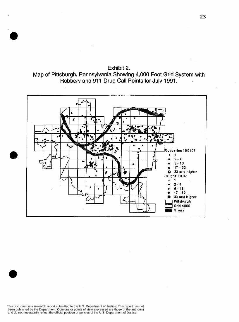
0 Leading indicators defined in Exhibit 3 - We had crime analysts from the
Pittsburgh and Rochester, NY Police Departments review all non-part 1 crime
codes and all CAD codes to suggest potential leading indicators for part 1 crimes
and do not necessarily reflect the official position or policies of the U.S. Department of Justice. been published by the Department. Opinions or points of view expressed are those of the author(s) This document is a research report submitted to the U.S. Department of Justice. This report has not

14
and drug CAD calls. Then, we had a noted criminologist, Dr. Jacqueline Cohen,
refine the list provided by the crime analysts to produce leading indicators for
part 1 property crimes, part 1 violent crimes, and CAD drug calls. All
independent variables in our leading indicator models are lagged one month.
Furthermore, our models also include spatial lags: independent variables lagged
one month and averaged over all contiguous neighbors of a grid. The spatial
lags allow for interactions over space, including effects of crime displacement,
spillover effects (e.g., of nearby drug dealing on robberies or burglaries), and
crime magnet effects such as holiday shopping, etc.
e Holt exponential smoothing with pooled seasonal factors, linear regression
leading indicator model, and neural network leading indicator model. The
linear regression is the simplest leading indicator model, while the neural
network model is an exploratory approach that automatically identifies and
estimates patterns in data?
rn Rollingfive years of estimation data for the Holt method, rolling three years of
estimation data for the regression model, and all historic data retained for the
neural network model. All methods forecast the same 36 month period, on the
one-month-ahead, rolling basis. Unlike the smoothing model, the regression
models cannot adapt to changing patterns in the data, but weight all data equally
regardless of age. Hence we chose a shorter time window (three years) for this
method to allow it to be somewhat adaptive. Indeed, over the 36 regression
models estimated per dependent variable, there were trends in independent
variable coefficients plotted as time series (e.g., shots fired increased in
importance for violent crimes). Neural networks are notorious for needing a lot
of data, so we retained all historic data rather than moving a fixed-length
window along.
There remains one more element to discuss about our experimental design, and that is the
framework for analysis. A common method of triggering decisions or attention in
monitoring systems is through rules based on threshold levels. For example, one rule is e
and do not necessarily reflect the official position or policies of the U.S. Department of Justice. been published by the Department. Opinions or points of view expressed are those of the author(s) This document is a research report submitted to the U.S. Department of Justice. This report has not
15
as follows: ifpart 1 violent crimes are forecasted to increase byfive or more in a grid
cell, then review that grid cell for possible action. Accepting this sort of approach
suggests a contingency table analysis of data. Elements of such an approach include:
A “positive” is any forecasted change of five or greater that is correct (the actual
change found later is five or more increase). This is a successful forecast.
A “false positive” is any forecasted change of five or greater that is incorrect (the
actual is four or less increase). This is a false alarm and is thus undesirable.
There are also “negatives” and “false negatives”, analogous to the positives but
for cases requiring no action. A false negative is a missed problem needing
attention and thus is undesirable.
The objective is to maximize positives and negatives to the extent existing in the
data, and thus minimizing false positives and false negatives.
We suggest that the “bar” should not be very high for leading indicator models, for them
to be considered useful. Forecasted changes exceeding the threshold for attention are
relatively rare and should not be considered facts, but merely high quality leads. Large
changes are likely to be time series pattern changes that would otherwise be total
surprises, were it not for leading indicator forecasts. Perhaps 50 percent positives and 50
percent false positives may be deemed a success in this context.
Results
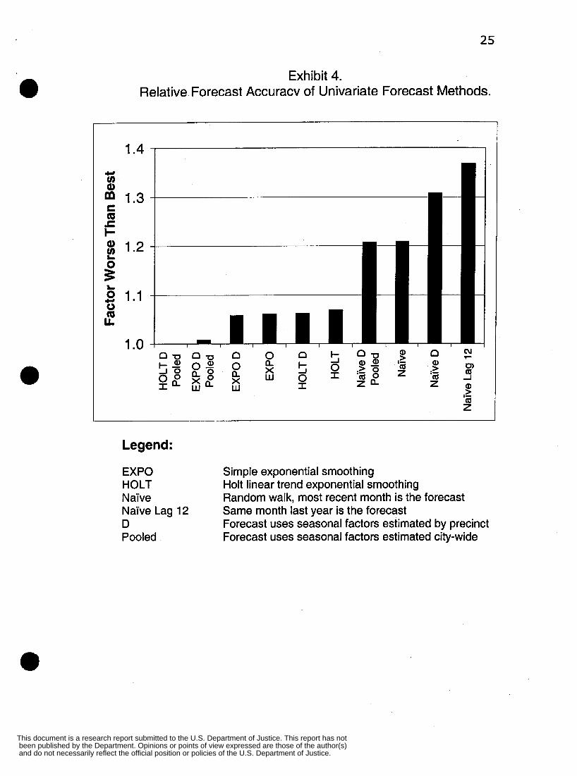
Two exhibits summarize the results of study 1 on univariate forecast methods. Exhibit 4
is a comparison of forecast accuracy across all crime types forecasted and all forecasts
made over the rolling horizon. The worst forecasting method is the police method, nahe
lag 12, which has 37 percent higher one-month-ahead forecast errors as measured by the
mean absolute percentage error (MAPE) than the overall best method, Holt exponential
smoothing with pooled seasonality. Using pair-wise comparison t-tests, the smoothing e
and do not necessarily reflect the official position or policies of the U.S. Department of Justice. been published by the Department. Opinions or points of view expressed are those of the author(s) This document is a research report submitted to the U.S. Department of Justice. This report has not

16
methods are significantly more accurate than the naTve methods at conventional levels,
and the pooled seasonality versions of smoothing methods are significantly more accurate
than those with seasonality estimated by precinct. In the tradeoff between more
homogeneous seasonality estimates (tailored by precinct) versus increased reliability
through pooled seasonal estimates (using city-wide data), Exhibit 4 and corresponding
statistical tests show that pooling yields higher forecast accuracy. Hence our current
research is pursuing more sophisticated methods of pooling data for seasonality factors.
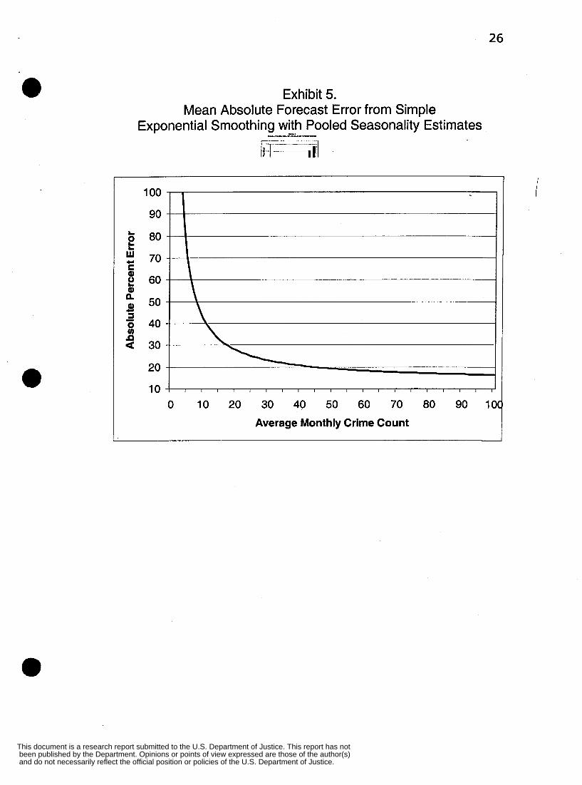
Exhibit 5 shows the average relationship between MAPE forecast error obtained from the
simple exponential smoothing method with pooled deseasonalization (EXPO D Pooled)
and average monthly crime count of precincts. There is a “knee of the curve”,
represented by an inverse relationship between MAPE forecast accuracy and average
crime count per month. Below average crime counts of around 30 per month, forecast
errors increase rapidly. At 30 or more, MAPE’s are approximately 20 percent. This level
of accuracy is acceptable for many purposes. The curve in Exhibit 5 is the result of a
multiple regression model for forecast absolute percentage error as explained by fixed
effects for precinct and crime type plus time series characteristics of data (magnitude of
time trend and seasonality), in addition to the inverse of average crime count. Only the
inverse of average crime count and the dummy variable for simple assaults were
statistically significant, providing evidence that crime scale is the major factor in
determining forecast error.
In summary, we find that exponential smoothing forecasts provide adequate accuracy for
the hotter crime areas. Pooled seasonality estimates, made with city-wide data contribute
to increased forecast accuracy. The next question is whether leading indicator forecast
models can improve over the best univariate forecasts for large changes in crime. In
answer to this question, we shall see that the leading indicators are best at forecasting
large crime decreases for all three crime types. For large crime increases, only the neural
network model for violent crimes was a successful forecaster. Future work introducing
census and land use data, and more sophisticated models should improve leading a
and do not necessarily reflect the official position or policies of the U.S. Department of Justice. been published by the Department. Opinions or points of view expressed are those of the author(s) This document is a research report submitted to the U.S. Department of Justice. This report has not

indicator forecasts. Also, forecasts for periods with crime increases (e.g., early 1990s)
might provide a better test bed for forecasting crime increases than our experiments in the
mid to late 1990s when crime decreased and leveled off.
a
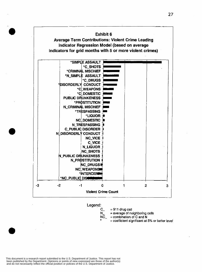
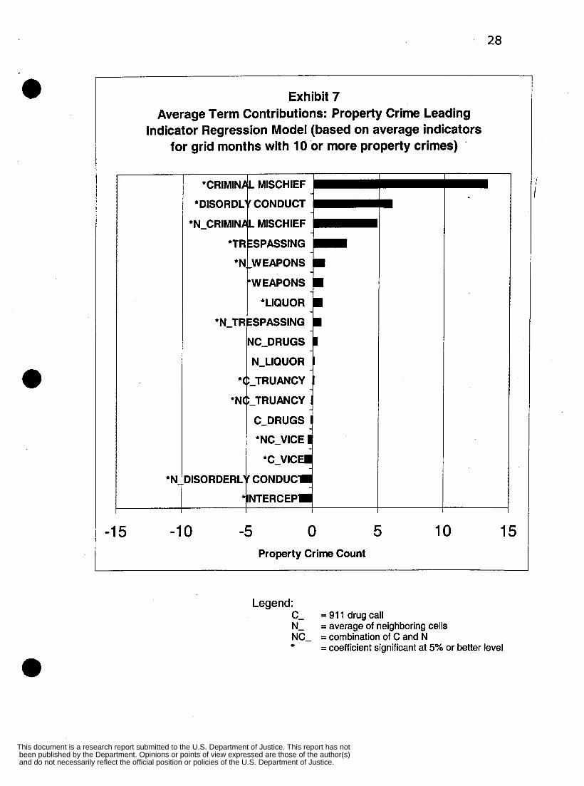
Exhibits 6 through 8 provide a summary of leading indicator models estimated by least
squares regression. In the rolling forecast experiments, we estimated a series of 36
regression models for each crime variable, each with three years’ data. We would
estimate a model, make one-step-ahead forecasts for all grid cells, drop the oldest
month’s data and add a new month’s data, and repeat the cycle. For exposition purposes,
we report here on a single regression model for each crime variable estimated over the
period of 1993-1998. Each of the bar charts in these figures was obtained by first
averaging the leading indicators across active grid cells, defined to be cells with average
dependent variable crime counts of five or more for violent crimes and drug calls, and 10
or more for property crimes. Then we multiplied the averaged leading indicators by
estimated regression coefficients, with the results displayed as bar charts. The result is
the average contribution of each term to a forecasted change in crime counts. a For part 1 violent crimes (Exhibit 6) , simple assaults in the same grid cell dominate other
leading indicators; however, a number of other leading indicators contribute significantly
including CAD shots fired, criminal mischief, simple assaults in neighboring grid cells,
CAD drug calls, disorderly conduct, and CAD weapons calls. There are fewer important
leading indicators for part 1 property crimes (Exhibit 7). Criminal mischief has the
largest impact, with disorderly conduct next, followed by criminal mischief in
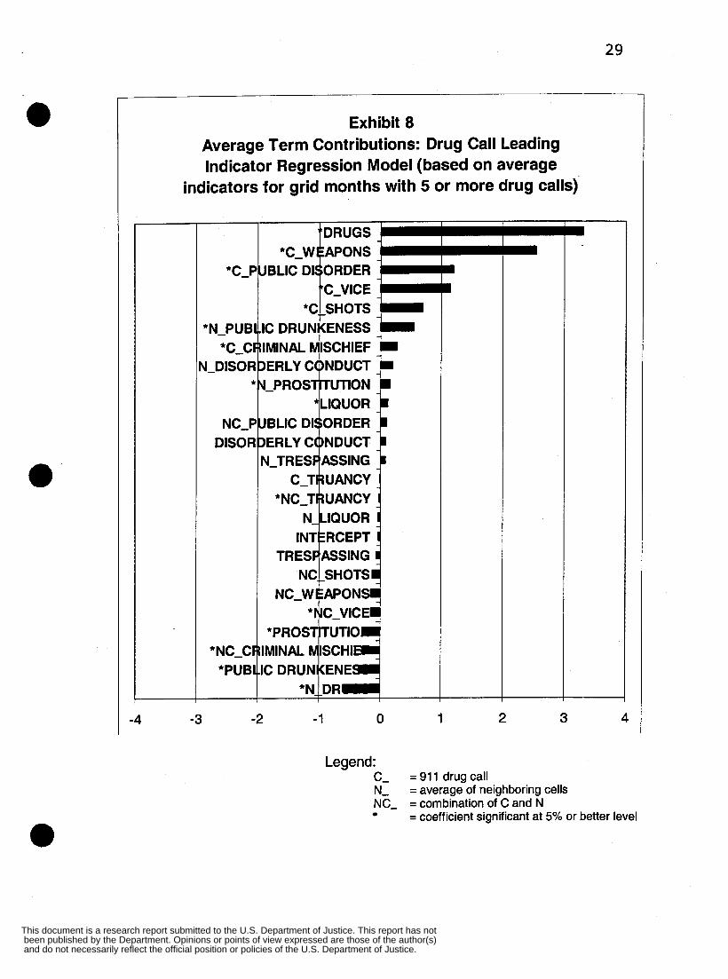
neighboring grid cells, and then trespassing. Finally, for CAD drug calls (Exhibit 8),
drug offenses (which correspond closely to drug arrests) dominates, showing a
persistence of drug dealing in place, followed by CAD weapons calls, CAD public
disorder calls, CAD vice calls, and CAD shots fired. The leading indicator models are all
highly statistically significant and make reasonable sense.
and do not necessarily reflect the official position or policies of the U.S. Department of Justice. been published by the Department. Opinions or points of view expressed are those of the author(s) This document is a research report submitted to the U.S. Department of Justice. This report has not
18
Finally, are results of the forecast experiments, in Exhibits 9 through 11. Note that the
order of presentation progresses from the best performing models (for violent crimes) to
worst performing models in terms of forecast accuracy. Overall, there is only moderate
success for the current models. Note also that comparison of alternative methods using
contingency table analysis is complex, so the reader will have to follow the text carefully
in order to understand these exhibits.
First is the case of part 1 violent crimes in Exhibit 9. There were 92 cell-months with
large decreases of five or more violent crimes. The regression leading indicator model
made a total of 64 forecasts of five or more decrease in violent crimes. Of these, the
regression model identified 38 correctly (41.3 percent positives = 100x38/92), but had 26
false positives (40.6 percent of positive forecasts = 100x26/64). So, 41.3 percent of the
time that the regression model forecasted a large crime decrease, it was right (positives),
but 40.6 percent of positive forecasts cried wolf (were false alarms). The regression
results are statistically better than those for the neural network leading indicator model
and univariate method.
There were 58 cases of large increases in violent crimes (five or more per grid-month).
The neural network leading indicator model made a total of 74 forecasts of five or more
increase in violent crimes. The neural network leading indicator model identified 22 (38
percent = lOOx22/58) of these, but also made 52 false positives (70 percent of all positive
forecasts = lOOx52/74). The neural network results are significantly better than the
others. Evidently, there are nonlinear components of the leading indicator model that the
neural network was able to find on its own.
i
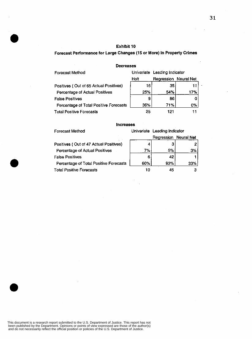
The results for property crimes are in Exhibit 10. Again, the regression model is best at
identifying large decreases, finding 35 (54 percent) out of 65, but with 86 (71 percent)
false positives. The neural network only found 11 (17 percent) of the large decreases, but
had no false positives. Also, the univariate method found only 16 (25 percent) of the e
and do not necessarily reflect the official position or policies of the U.S. Department of Justice. been published by the Department. Opinions or points of view expressed are those of the author(s) This document is a research report submitted to the U.S. Department of Justice. This report has not

19
large decreases, but only had 9 (36 percent of positive forecasts) false positives. None of
the methods were successful in identifying the 47 large increases in property crimes.
This is an area that needs improvement.
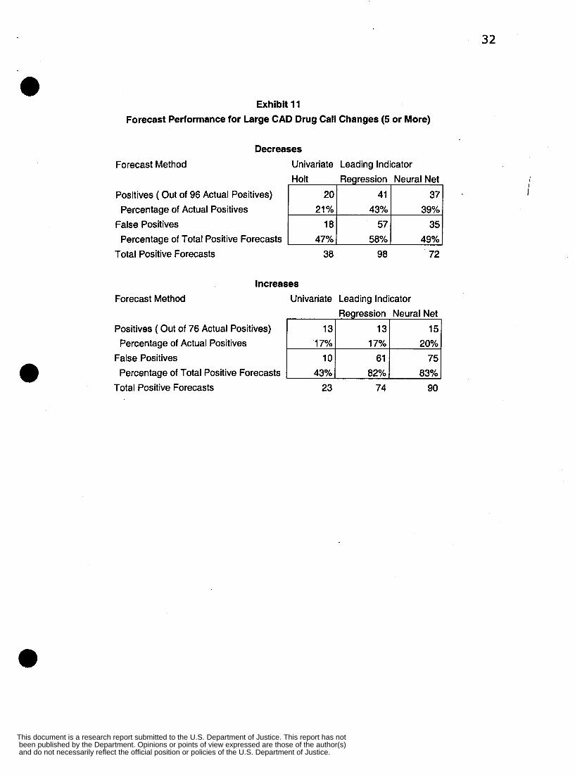
In Exhibit 11, both leading indicator models were successful in identifying large
decreases in CAD drug calls. Best was the regression model, finding 41 (43 percent) of
the 96 actual large decreases. The regression model had 57 (58 percent) false positives.
The results are statistically significant, that leading indicators are better than the
univariate model. On large increases, all methods are weak on identifying and
discriminating these changes.
In summary, the leading indicators are best at forecasting large crime decreases for all
three crime types. For large crime increases, only the neural network model for violent
crimes was a successful forecaster. Additional work needs to be done on forecasting
increases for property crimes and drug calls.
Recornmenda tions
First are recommendations for police:
1. Forecast major crimes one month ahead for precincts, car beats, and uniform
grid cells as small as approximately I O blocks on a side. These are the
requirements of crime forecasting for tactical deployment of police. Precincts and
car beats are important for administrative purposes. Grid cells are the easiest
areal units to interpret visually and provide the finest-grainded results. Additional
recommendations below provide details and caveats.
2. Stop using the same month from last year as the basis for evaluating police
perjGormance in a month this year. This method is by far the worst method that
we evaluated for forecasting one month ahead. A better practice would be to use
and do not necessarily reflect the official position or policies of the U.S. Department of Justice. been published by the Department. Opinions or points of view expressed are those of the author(s) This document is a research report submitted to the U.S. Department of Justice. This report has not
20
forecast prediction intervals or methods from quality control to determine if a
recent month were unusual - significantly higher or lower than the established
trend. Such a practice would evaluate recent police actions, to provide evidence
of crime pattern changes.
3. Estimate seasonal factors for use in crime analysis. Estimate seasonal factors
using multiplicative, classical decomposition from jurisdiction-wide data. Study
the seasonal factors and corresponding crime maps for peak crime seasons and
patterns.
4. Make univariate forecasts for crime types and areas that have average monthly
crime counts of 30 or more. Deseasonalize data using Classical Decomposition.
Use Holt exponential smoothing for time trend estimation and forecasting. With
crime counts of 30 or more, the average absolute forecast error is around 20
percent (too high or too low). If average crime counts are much lower, forecast
errors rise rapidly. The univariate methods provide business-as-usual forecasts,
extrapolating established trends and seasonality.
5 . Develop and refine a set of leading indicator crimes and CAD calls. Our research
proposed sets of part 2 crimes and CAD call types as leading indicators of part 1
violent and property crimes, and CAD drug calls. Our experimental research
demonstrated that leading indicators are significantly better than univariate
forecast methods for cases with large crime count decreases and for violent crime
increases in the forecast period. Current and future research promises to improve
leading indicator forecast models by adding more explanatory factors; for
example, demographic and land use variables.
6. Use leading indicators in crime mapping. Plot choropleth maps of crime
forecasts as an early warning map. Allow the analyst to zoom into the individual
leading indicator points and major crimes to diagnose a forecast.
Recommendations for researchers include:
1. Evaluate crime forecasts using the rolling horizon experimental design. Obtain
sufficiently long data sets so that models can be reliably estimated and forecasted
and do not necessarily reflect the official position or policies of the U.S. Department of Justice. been published by the Department. Opinions or points of view expressed are those of the author(s) This document is a research report submitted to the U.S. Department of Justice. This report has not

21
2.
3.
4.
over a long enough series of forecast origins. We used eight years of data. We
used a five-year rolling window for univariate forecasts, a three-year ahead
rolling window for multiple regression leading indicator model estimation, and
made a series of 36 one-month-ahead forecasts.
Compare advanced to simple forecast methods. Compare forecast accuracy of
leading indicator models to the best univariate method. In order to recommend a
leading indicator model, it needs to forecast more accurately than the simpler,
business-as-usual univariate method. Expect the leading indicator models to
perform better than univariate methods for large changes in crime counts, large
increases or decreases.
Evaluate forecast accuracy in intervals corresponding to threshold decision rules.
Example decision rules might be: a. do nothing different (low change forecasted),
b. be vigilant (medium change forecasted), and c. intervene (large change
forecasted). Evaluate alternative models within forecasted change intervals using
pair-wise comparisons to control for lack of independence of forecasts.
Consider advanced leading indicator models forfuture work. The list of potential
extensions and improvements for leading indicator models includes: consider
vector autoregressive models to identify lags longer than one month, include
nonlinear terms in the model specification (based on neural network results), use
census and land use features to add fixed effects components and better fit city-
wide data, weight averages for spatial lags based on nature of relationship
between neighboring cells, and build different models for crime increases versus
decreases.
i
and do not necessarily reflect the official position or policies of the U.S. Department of Justice. been published by the Department. Opinions or points of view expressed are those of the author(s) This document is a research report submitted to the U.S. Department of Justice. This report has not
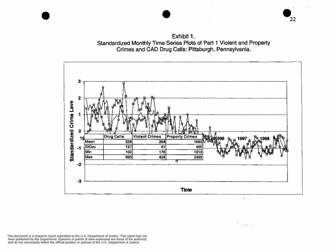
Exhibit 1. Standardized Monthly Time Series Plots of Part 1 Violent and Property
Crimes and CAD Drug Calls: Pittsburgh, Pennsylvania.
3
2
1
0 1
-1
-2
-3
Time
and do not necessarily reflect the official position or policies of the U.S. Department of Justice. been published by the Department. Opinions or points of view expressed are those of the author(s) This document is a research report submitted to the U.S. Department of Justice. This report has not
23
Exhibit 2. Map of Pittsburgh, Pennsylvania Showing 4,000 Foot Grid System with
Robbery and 91 1 Drua Call Points for July 1991.
and do not necessarily reflect the official position or policies of the U.S. Department of Justice. been published by the Department. Opinions or points of view expressed are those of the author(s) This document is a research report submitted to the U.S. Department of Justice. This report has not
24
Exhibit 3 Definition of Leading Indicators by Dependent Variable Type
and do not necessarily reflect the official position or policies of the U.S. Department of Justice. been published by the Department. Opinions or points of view expressed are those of the author(s) This document is a research report submitted to the U.S. Department of Justice. This report has not
25
Exhibit 4. Relative Forecast Accuracv of Univariate Forecast Methods.
1.4 I I w cn
1.3 r I- $ 1.2
L 2 1.1
1 .o
Legend:
EXPO Simple exponential smoothing HOLT Nai’ve Naive Lag 12 D Pooled
Holt linear trend exponential smoothing Random walk, most recent month is the forecast Same month last year is the forecast Forecast uses seasonal factors estimated by precinct Forecast uses seasonal factors estimated city-wide
and do not necessarily reflect the official position or policies of the U.S. Department of Justice. been published by the Department. Opinions or points of view expressed are those of the author(s) This document is a research report submitted to the U.S. Department of Justice. This report has not
26
Exhi bit 5. Mean Absolute Forecast Error from Simple
Exponential Smoothing with -. Pooled Seasonality Estimates -.--.-.-.... -1
100
90
80
10 1 1 l 1 1 1 1 1 1 1 1 1 1 1 1 1 1 1 1 I
0 10 20 30 40 50 60 70 80 90 10( Average Monthly Crime Count
and do not necessarily reflect the official position or policies of the U.S. Department of Justice. been published by the Department. Opinions or points of view expressed are those of the author(s) This document is a research report submitted to the U.S. Department of Justice. This report has not
27
Exhibit 6 Average Term Contributions: Violent Crime Leading
Indicator Regression Model (based on average indicators for grid months with 5 or more violent crimes)
-3 -2 -1 0 1 2 3
Violent Crime Count
Legend: C- = 91 1 drug call N- = average of neighboring cells NC- = combination of C and N
= coefficient significant at 5% or better level
and do not necessarily reflect the official position or policies of the U.S. Department of Justice. been published by the Department. Opinions or points of view expressed are those of the author(s) This document is a research report submitted to the U.S. Department of Justice. This report has not
28
~~
*CRIMINAL
*DISORDLY
"NCRIMINAL
*N-TR
*C:
NSORDERL"
Exhibit 7 Average Term Contributions: Property Crime Leading
Indicator Regression Model (based on average indicators for grid months with 10 or more property crimes)
MISCHIEF - - CONDUCT
-
MISCHIEF - *TRESPASSING -
-
*N.-WEAPONS D
*WEAPONS I
*LIQUOR
ESPASSING
NC-DRUGS B N-LIQUOR I
- TRUANCY I
-
-
-
-
-
- *NC:-TR UANCY
C-DRUGS
* NC-VICE
*C-VICEm - CONDUC-
*INTERCEPW I
-
-1 5 -1 0 -5 0 5 10 15 Property Crime Count
Legend: C- = 91 1 drug call N- = average of neighboring cells NC- = combination of C and N
= coefficient significant at 5% or better level
and do not necessarily reflect the official position or policies of the U.S. Department of Justice. been published by the Department. Opinions or points of view expressed are those of the author(s) This document is a research report submitted to the U.S. Department of Justice. This report has not
29
Exhibit 8 Average Term Contributions: Drug Call Leading Indicator Regression Model (based on average
indicators for grid months with 5 or more drug calls)
*C-F
*N-PUB *c-c
4-DISOF i
NC-F DISOF
*PROS UTI0 9 * $ R J
*NC-C IMINAL ISCHI *PUB ICDRUN ENE
-4 -3 -2 -1 0 1 2 3 4
Legend: C- = 911 drug call N- = average of neighboring cells NC- = combination of C and N
= coefficient significant at 5% or better level
and do not necessarily reflect the official position or policies of the U.S. Department of Justice. been published by the Department. Opinions or points of view expressed are those of the author(s) This document is a research report submitted to the U.S. Department of Justice. This report has not

30
Positives ( Out of 58 Actual Positives) Percentage of Actual Positives
Percentage of Total Positive Forecasts False Positives
Exhibit 9
Forecast Performance for Large Changes (5 or More) in Violent Crimes
4 4 22 7% 7% 38% 14 8 52
78% 67% 70%
Decreases
Forecast Method
Positives ( Out of 92 Actual Positives)
False Positives
Total Positive Forecasts
Percentage of Actual Positives
Percentage of Total Positive Forecasts
Univariate
22 24%
11 33%
33
Leading Indicator Regressif, Neural N;!
41 ?‘o 22%
64 28 41 % 29%
i
and do not necessarily reflect the official position or policies of the U.S. Department of Justice. been published by the Department. Opinions or points of view expressed are those of the author(s) This document is a research report submitted to the U.S. Department of Justice. This report has not
31
16 35 11 25% 54% 17%
9 86 0 36% 71 % 0%
Exhibit 10
Forecast Performance for Large Changes (15 or More) in Property Crimes
.
Decreases
Positives ( Out of 47 Actual Positives) Percentage of Actual Positives
Percentage of Total Positive Forecasts False Positives
Forecast Method
4 3 2 7% 5% 3%
6 42 1 60% 93% 33%
Positives ( Out of 65 Actual Positives)
False Positives
Total Positive Forecasts
Percentage of Actual Positives
Percentage of Total Positive Forecasts
and do not necessarily reflect the official position or policies of the U.S. Department of Justice. been published by the Department. Opinions or points of view expressed are those of the author(s) This document is a research report submitted to the U.S. Department of Justice. This report has not
32
Positives ( Out of 76 Actual Positives)
False Positives Percentage of Actual Positives
Percentage of Total Positive Forecasts
Exhibit 11 Forecast Performance for Large CAD Drug Call Changes (5 or More)
13 13 15 17% 17% 20%
10 61 75 43% 82% 83%
Decreases
Forecast Method
Positives ( Out of 96 Actual Positives)
False Positives
Total Positive Forecasts
Percentage of Actual Positives
Percentage of Total Positive Forecasts
Univariate Holt
20 21 %
18 47%
38
Leading Indicator Regressi;7 I Neural N;i
43% 39%
58% 49% 98 72
and do not necessarily reflect the official position or policies of the U.S. Department of Justice. been published by the Department. Opinions or points of view expressed are those of the author(s) This document is a research report submitted to the U.S. Department of Justice. This report has not
33
Glossary
Areal Unit
AutoregressiveLMoving Average Models Classical Decomposition Coun terfac tual Forecast
Dependeen t Variable
Deseasonalizing Data
Exponential Smoothing
Extrapolation Forecast Horizon
Hold-Out Sample
Holt Exponential Smoothing Independent Variable
Lag - Spatial
Lag - Time
Leading Indicator Forecast Models
Least Squares Regression Model
Spatial area which is a unit of observation (e.g., precinct, census tract) Complex univariate forecast model popular in the 1970s and 1980s also known as BodJenkins forecast models
Simple method used to estimate seasonal factors An extrapolative forecast used as the basis for comparison or evaluation Variable of interest for decision making (e.g., number of robberies in a precinct per month) Either subtracting additive seasonal estimates or dividing by multiplicative seasonal estimates to remove seasonal variations from time series data
An extrapolation procedure used for forecasting. It is a weighted moving average in which the weights are decreased exponentially as data becomes older. A forecast based only on earlier values of a time series The number of periods from the forecast origin to the end of the time period being forecast. Data not used in constructing a forecast model but are forecasted using the model, providing the basis for validationof the model in forecast experiments.
Exponential smoothing model estimating a time trend Variable used to explain or predict the dependent variable (e.g., a time index or number of leading indicator crimes) Often the average or sum of an independent variable in areal units surrounding the areal unit being considered as an observation A difference in time between an observation and a previous observation; sometimes used for independent variables that are leading indicators (e.g., last month’s shots fired CAD calls may predict this months aggravated assaults)
A multivariate time series model in which the independent variables are leading indicators (e.g., this month’s shots fired CAD calls and simple assaults may predict next month’s part 1 violent crimes)
The standard approach to regression analysis wherein the goal is to minimize the sum of squares of the deviations between actual and predicted values in the calibration data.
The average of a variable in a sample of data
I
Mean
and do not necessarily reflect the official position or policies of the U.S. Department of Justice. been published by the Department. Opinions or points of view expressed are those of the author(s) This document is a research report submitted to the U.S. Department of Justice. This report has not

34
Mean Absolute Percentage Error (MAPE)
Multivariate Model
Nai’ve Forecast
Neural Network Model
Noise
Optimization Procedure
Pairwise Comparison t-Tests
Pooled Estimates
Random Walk
Rolling Horizon Forecast Experiment
Seasonality
Seasonality - Additive
Seasonality - Multiplicative
Short-term Forecasts Simple Exponential Smoothing
Smoothing Parameters
=Sum of 100’Absolute Value (Actual Value - Forecast Value)/Actual Value over a set of forecasts; yields average percentage errors with signs removed (e.g., 20% MAPE means that on average a forecast is 20% too high or too low, off by 20%)
Model in which the dependent variables is explained by two ro more independent variables Forecast method that does not use any averaging of data to remove effects of noise A complex multivariate model that is capable of self-learning intricate mathematical patterns in data The random, irregular, or unexplained component in a measurement process. A mathematical set of steps that search for the best values for a model based on training datra A statistical test that compares pairs of alternative estimates or forecasts for the same quantity Estimates that use data from a group of areal units instead only the real unit being modeled (e.g., a univariate time series model for a precinct that uses seasonal factors estimated form all precincts in a jurisdiction)
A model in which the latest value in a time series is used as the forecast for all periods in the forecast horizon. An experimental design for evaluating alternative forecast models using training data and hold-out samples in which the forecaster makes several forecasts as if time is passing and new forecasts must be made when new data arrives; the design gets the most out of a time series data set by making many forecasts at different points in time, thus yielding many forecast errors for analysis and summary. Systematic cycles within the year, typically caused by weather, culture, or holidays Seasonal estimates that are added to a trend model to represent seasonality; generally not valid for use across areal units because of differences in magnitudes of the dependent variable (e.g., high versus low crime areas)
Seasonal estimates that are mutiplied times a trend model to represent seasonality; are factors suc as 0.8 or 1.3 that are dimensionless and thus work well across areal units (e.g., high and low crime areas)
Generally forecasts with horizons less than a year Exponential smoothing model estimating only a moving average and is only capable of a horizontal forecast over time with no time trend
One to three parameters that control how quickly an exponential smoothing model can adapt to time series pattern changes, generally estimated using an optimization procedure
and do not necessarily reflect the official position or policies of the U.S. Department of Justice. been published by the Department. Opinions or points of view expressed are those of the author(s) This document is a research report submitted to the U.S. Department of Justice. This report has not
35
Standard Deviation
Standarized Data
Step Jump
Time Series
Time Series Patterns
Time Trend
Training Data
Turning point Uni vari ate Forecast Methods
Variance
The square root of the variance. A summary statistic, usually denoted by s, that measures variation in the sample Data which have been transformed to have a mean of zero and standard deviation of one A sudden and relatively large change in a time series pattern that moves the entire pattern up or down relative to the old pattern
Data collected over time and aggregated to counts or sums by time period (e.g., weeks, months, quarters, years) Systematic changes in a quantity as a function of time such as linear trend, seasonality, or consistent under or over estimates Part of a time series model in which an estimated amount is added to or subtracted from the model with every increase in time (e.g., month, quarter, or year)
Data used to calibrate a model so that the model can estimate and forecast quantities The point at which a time series changes direction Forecast methods for models using only the dependent variable time series with a time index as the basis for independent variables A measure of variation equal to the mean of the squared deviations from the mean
and do not necessarily reflect the official position or policies of the U.S. Department of Justice. been published by the Department. Opinions or points of view expressed are those of the author(s) This document is a research report submitted to the U.S. Department of Justice. This report has not
36
See Dodenhoff, P.C., “LEN Salutes its 1996 People of the Year, the NYPD and its Compstat Process,” Law Enforcement News, Vol. XXII, No. 458, 12/31/1996, John Jay College of Criminal Justice; Anderson, D.C., Crime Control by the Numbers, Ford Foundation Report, Winter 2001; Rossmo, K. 1999, Geographic Profiling, CRC Press, New York.
For a review of spatial econometrics applied to crime analysis, see Anselin, L., J. Cohen, D. Cook, W.L. GOK, and G. Tita, “Spatial Analysis of Crime,” in Duffee, D. [ed.], Volume 4. Measurement and Analysis of Crime and Justice, Criminal Justice 2000, July 2000, NCJ 18241 1, pp 213-262.
See, for example, Makridakis, S., A. Andersen, R. Carbone, R. Fildes, M. Hibon, R. Lewandowski, J. Newton, E. Parzen, & R. Winkler (1982), ‘The accuracy of extrapolation (time series) methods: results of forecasting competition, ” Journal OfForecasting 1,111-153 and Makridakis Spyros, Hibon MichiYe (ZOOO), The M3-Competition: results, conclusions and implications, International Journal Of Forecasting (16) 4 pp. 45 1476.
Makridakis, S. and Wheelwright S.C. (eds) 1987, The Handbook of Forecasting, Wiley, NY, pages 173- 195,220; Yaffee, R. 2000, Introduction to Time Series Analysis and Forecasting with Applications of SAS and SPSS, Academic Press, San Diego, pages 23-38; Bowerman, B.L. and O’Connell, R.T., Forecasting and Time Series: An Applied Approach 1993, Duxbury Press, Belmont CA, pages 355-370,379-386,400- 403.
The New York Police Department uses this method as do many other police departments. See httr,://www.nvc.gov/html/nv~d/htmYchfdeDt/Drocess.html.
For example, see Kelling, G. L. and C.M. Coles (1996), Fixing Broken Windows: Restoring Order and Reducing Crime in Our Communities, NY: Free Press and Cohen, L.E. and M. Felson (1979), “Social Change and Crime Rate Trends: A Routine Activity Approach,” American Sociological Review 44,588-607. ’ Note that inclusion of robbery in the property crime aggregate has little effect on that aggregate, but the opposite is true for violent crimes. Robbery is a relatively low incidence crime, but so are most part 1 violent crimes.
minimized one-step-ahead, mean squared forecast errors within the estimation sample.
Crime Mapping, Crime Prevention. D. Weisburd, and T. McEwen (eds) Money, NY: Criminal Justice
For detailed descriptions of exponential smoothing and classical decomposition see the following:
We used a full grid search of each smoothing parameter in increments of 0.1 from 0.1 to 0.9 and
We used the same model as in Olligschlaeger, A. M. 1997. Artificial neural networks and crime mapping.
Press. PRuixH-rY OF
National Criminal Justice Reference Senrice (NCJRS) Box 6000 Rockviile, MD 20849-6000 _4y”-
and do not necessarily reflect the official position or policies of the U.S. Department of Justice. been published by the Department. Opinions or points of view expressed are those of the author(s) This document is a research report submitted to the U.S. Department of Justice. This report has not


![Forecasting Crime with Deep Learning - arXiv · crime data. We make use of weather data, census data, and public transportation data on top of the crime reports. Cohn [4] establishes](https://img.pdfslide.net/doc/110x75/5f66a77ca7fa7c529521e9f8/forecasting-crime-with-deep-learning-arxiv-crime-data-we-make-use-of-weather.jpg)