Artifact Detection and QA Manual Susan Whitfield-Gabrieli MIT

The zip / tar.gz files include the tool's Matlab source files and documentation. To install, simply extract the files and place them somewhere in your matlab path. MATLAB and SPM are required. The code is compatible with SPM99/2/5/8 and Analyze (.img) and NIFTI (.img/.nii) format images. Motion parameters can be specified either as .txt files (SPM) or .par files (FSL). The software was developed by Susan Whitfield-Gabrieli, Shay Mozes and Alfonso Nieto Castañón. Satra Ghosh has developed python scripts which are compatible with 4-d Nifti formats (Please see RAPIDART at NTRIC).

Introduction The ARtifact detection Tools (ART) software package offers a set of tools that facilitates the identification of outlier values in fMRI time series that likely reflect artifacts and provides diagnostics tools which assist in appropriate design specification and model estimation. Specifically it offers 1) automatic and manual detection of global mean intensity and motion outliers in fMRI data that may be omitted from subsequent statistical analyses, interpolated or deweighted in the GLM; 2) methods for diagnosing the degree of stimulus correlated motion in order to determine whether or not to include motion as confounds in the GLM; 3) methods for determining task correlation with global brain signal, in order to decide on global scaling options; 4) superposition of the experimental design on the time series for visual inspection; and 5) calculation of the power spectra of the experimental paradigm, as well as the motion, in order to allow users to select an appropriate high pass filter that does not filter out the frequencies associated with the task (Fig 1).

Fig. 1 Art tool.The ARtifact detection Tools (ART) software package allows detection of outliers in global signal intensity as well as translation and rotational movement parameters. The art tool also allows data exploration options.

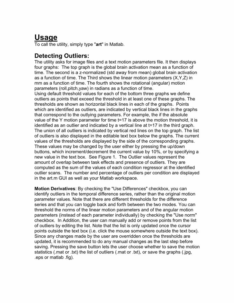
Usage To call the utility, simply type "art" in Matlab. Detecting Outliers: The utility asks for image files and a text motion parameters file. It then displays four graphs: The top graph is the global brain activation mean as a function of time. The second is a z-normalized (std away from mean) global brain activation as a function of time. The Third shows the linear motion parameters (X,Y,Z) in mm as a function of time. The fourth shows the rotational (angular) motion parameters (roll,pitch,yaw) in radians as a function of time. Using default threshold values for each of the bottom three graphs we define outliers as points that exceed the threshold in at least one of these graphs. The thresholds are shown as horizontal black lines in each of the graphs. Points which are identified as outliers, are indicated by vertical black lines in the graphs that correspond to the outlying parameters. For example, the if the absolute value of the Y motion parameter for time t=17 is above the motion threshold, it is identified as an outlier and indicated by a vertical line at t=17 in the third graph. The union of all outliers is indicated by vertical red lines on the top graph. The list of outliers is also displayed in the editable text box below the graphs. The current values of the thresholds are displayed by the side of the corresponding graphs. These values may be changed by the user either by pressing the up/down buttons, which increment/decrement the current value by 10%, or by specifying a new value in the text box. See Figure 1. The Outlier values represent the amount of overlap between task effects and presence of outliers. They are computed as the sum of the values of each condition regressor at the identified outlier scans. The number and percentage of outliers per condition are displayed in the art.m GUI as well as your Matlab workspace. Motion Derivatives: By checking the "Use Differences" checkbox, you can identify outliers in the temporal difference series, rather than the original motion parameter values. Note that there are different thresholds for the difference series and that you can toggle back and forth between the two modes. You can threshold the norms of the linear motion parameters and of the angular motion parameters (instead of each parameter individually) by checking the "Use norm" checkbox. In Addition, the user can manually add or remove points from the list of outliers by editing the list. Note that the list is only updated once the cursor points outside the text box (i.e. click the mouse somewhere outside the text box). Since any changes made by the user are overridden once the thresholds are updated, it is recommended to do any manual changes as the last step before saving. Pressing the save button lets the user choose whether to save the motion statistics (.mat or .txt) the list of outliers (.mat or .txt), or save the graphs (.jpg, .eps or matlab .fig).

Data Exploration: Design: The "Show Design" checkbox. When this checkbox is checked, the task conditions from the design matrix are superimposed on the signal intensity time series graph. This might help identify correlations between the motion or the task and the experimental design. This design matrix is obtained from the SPM.mat file specified by the user. This is show below.

Fig. 2 Task design Pressing the small '+' button on the left side of the z-graph will plot it in a separate window (shown below).

Fig. 3 Task design blown up

Stimulus correlated motion: The "motion-task corr." checkbox displays in a new window a matrix where the rows correspond to the conditions, the columbs correspond to the motion parameters and the colors correspond to the correlation coefficient between them. It thus provides an intensity map of the correlations between the task conditions and motion parameters for each session.

Fig. 4 Stimulus Correlated Motion Note: It is better to use a design matrix (“template design matrix”) where the motion parameters are not considered as covariates, since the motion parameters are shown anyway. Global Signal: Similarly, the "signal-task corr." checkbox displays in a new window an intensity map of the correlations between the global signal and task conditions for each session.

Power Spectra: The "Show Spectrum" displays the power spectrum of the task conditions and motion parameters in a new window (each session has its own graph). The highpass cutoff frequency is also displayed. The user may choose which parameters to display by (un)checking the appropriate checkboxes. Note: It is far better to use a design matrix where the motion parameters are not considered as covariates, since the motion parameters are shown anyway.

Fig. 5 Power Spectra

The default high pass filter cutoff in SPM2 and higher is .01 Hz (128 seconds) and represents the inflection point of 1/f and white noise. An apparent small change in this cutoff can result in large differences in your results. Above you see activation maps in the upper right hand corner: top has hpf cutoff of .01 hz and the lower activation map is the result of a hpf cutoff of .02 hz. You can see that a cutoff of .02 hz filtered out the task activation. It is thus wise to plot the power spectra of your design matrix and observe where the fundamental frequencies of your task are wrt your choise of hpf cutoff.

Fig. 6 Power Spectra of task conditions: allows you to select appropriate high pass filter cutoff.

Saving Results: You can choose to save the outliers (combined global mean intensity as well as motion), the number of outliers per condition, the motion summary, the correlation coefficients, the jpegs of the results and SPM regressors for inclusion in first level GLM.

Fig. 7 Save options You can omit these bad time points in the GLM by including a single regressor for each scan you want to remove, with a 1 for the scan you want to remove, and zeros elsewhere (See Fig. 7) Including parameters as covariates can increase sensitivity, especially in event related designs. However, if the motion parameters are correlated with the task conditions, including the parameters as covariates could eliminate task activation. In addition, beware of between group differences in SCM when comparing groups. (Bullmore 1999) as this can result in artifactual between-group differences. One possible method of addressing this situation would be via

2nd level Ancova, where the amount of scm for each subject is entered as a nuisance regressor. Note: Finally do top down QA on first and second level statistics. Superimpose the mask (mask.img) image on a high resolution anatomy image to see which voxels were included in the analysis. The mask.img lives in the first level stats directory as well as the second level stats directory. The second level mask image is the intersection of all first level masks. Also, do a check registration in SPM of the ResMS.img, Mask.img, RPV.img and Tmaps of interest to discover further issues.