Artificial neural networks of soil erosion and runoff prediction at the

Artificial neural networks of soil erosion

and runoff prediction at the plot scale

P. Licznara, M.A. Nearingb,*

a Institute of Building and Landscape Architechture, Agriculture University, Wroclaw, PolandbUSDA-ARS-National Soil Erosion Research Laboratory, 1196 Soil Building,

Purdue University, West Lafayette, IN 47907, USA

Received 4 July 2001; received in revised form 7 August 2002; accepted 20 September 2002

Abstract

Neural networks may provide a user-friendly alternative or supplement to complex physically

based models for soil erosion prediction for some study areas. The purpose of this study was to

investigate the applicability of using neural networks to quantitatively predict soil loss from natural

runoff plots. Data from 2879 erosion events from eight locations in the United States were used.

Neural networks were developed for data from each individual site using only eight input

parameters, and for the complete data set using 10 input parameters. Results indicated that the neural

networks performed generally better than the WEPP model in predicting both event runoff volumes

and soil loss amounts, with exception of some small events where the negative erosion predictions

were not physically possible. Linear correlation coefficients (r) for the resulting predictions from the

networks versus measured values were generally in the range of 0.7 to 0.9. Networks that predicted

runoff and soil loss individually did not perform better than those that predicted both variables

together. The type of transfer function and the number of neurons used within the neural network

structure did not make a difference in the quality of the results. Soil loss was somewhat better

predicted when values were processed using a natural logarithm transformation prior to network

development. The results of this study suggest the possibility for using neural networks to estimate

soil erosion by water at the plot scale for locations with sufficient data from prior erosion monitoring.

D 2002 Elsevier Science B.V. All rights reserved.

Keywords: Soil erosion; Neural networks; WEPP; Natural runoff plots

0341-8162/02/$ - see front matter D 2002 Elsevier Science B.V. All rights reserved.

PII: S0341 -8162 (02 )00147 -9

* Corresponding author. Tel.: +1-765-494-8683; fax: +1-765-494-5948.

E-mail address: [email protected] (M.A. Nearing).

www.elsevier.com/locate/catena

Catena 51 (2003) 89–114

1. Introduction

Since the early 1990s, artificial neural networks’ popularity has been rising and they are

gaining new fields of implementation at a rapid rate. In general, neural networks may be

thought of as resembling to some extent the biological neural networks of the human brain.

They can analyze multi-source data sets and are considered as universal approximators.

Hornik (1991) has shown that the standard multi-layer, feed-forward network is able to

approximate any measurable function to any desirable degree of accuracy. Artificial neural

networks are being successfully used in many areas closely related to soil erosion. The

American Society of Civil Engineers (ASCE) Task Committee on Application of Artificial

Neural Networks in Hydrology (2000a) reports applications for rainfall-runoff modeling,

stream flow forecasting, ground water modeling, water quality, water management policy,

precipitation forecasting, hydrological time series, and reservoir operations. Surprisingly,

only a few articles describe results of artificial neural network implementation in erosion

research. In that area, artificial neural networks have been used mainly for classification of

erosion processes. Rosa et al. (1999) captured interactions between the land and land

management qualities and a vulnerability index to soil erosion in Andalucia region in

Spain by means of expert decision trees and artificial neural networks. Harris and

Boardmann (1998) used expert systems and neural networks as an alternative paradigm

to mathematical process-based erosion modeling for South Downs in Sussex, England.

However, we know of no publication describing quantitative prediction of soil loss and

runoff at the plot scale.

From the beginning of the soil erosion research, soil loss and runoff studies at the plot

scale have been of crucial importance. The extensive data from plot studies have formed

the basis of a number of empirical erosion models, e.g., the Universal Soil Loss Equation

(USLE) (Wischmeier and Smith, 1958, 1978) and its modified version—the Revised

Universal Soil Loss Equation (RUSLE) (Renard et al., 1991, 1996). The recent tendency

to move from using empirical erosion models to the more advanced, physically based or

theoretical ones capable of performing larger scale analyses does not reduce the important

and fundamental role of the plot scale studies. Results from those studies continue to

supply enormous amounts of information needed for model calibrations and evaluations.

The plot scale has proved to be optimal for the introduction of new erosion technologies

because of providing access to reliable and consistent erosion measurements and the large

numbers of data necessary to test new models (Nearing et al., 1999). For example, the

physically based model, the Water Erosion Prediction Project model (WEPP), described by

Lane and Nearing (1989) and by Ascough et al. (1997), was primarily evaluated on the

basis of the data from the natural runoff plots (Zhang et al., 1996).

In view of this and also the need for new better tools for predicting runoff and soil

erosion, this study examines the possibility of implementing artificial neural networks at

the plot scale. It presents a comparison study between results from erosion and runoff

procedures of the WEPP technology and from artificial neural networks. Measured versus

predicted values of the sediment load and runoff volumes are plotted, and linear regression

parameters are established for several data sets selected from eight sites located in the

eastern United States. Comparison between WEPP and neural networks of two specific

architectures were made for every site-specific set of data. Also, a more detailed

P. Licznar, M.A. Nearing / Catena 51 (2003) 89–11490

comparison study was made on the basis of the entire data set containing information from

all the plots combined. The impact of different network architectures and the data set

preparation technique for the prediction accuracy is presented. In most cases, the results

received from the neural networks were better than those from WEPP, although the neural

networks generally tended to under-predict runoff and soil loss values.

2. Material and methods

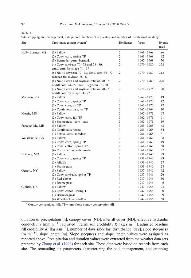
For the purpose of this study, runoff and soil loss data were selected from plots located

in eight sites in the eastern United States. The data represented a broad range of climatic

and physiographical conditions. It was the same data used previously by Zhang et al.

(1996) for WEPP evaluation, except that all the events yielding no soil loss or no runoff

were removed. Table 1 summarizes the data used, and further details may be found in

Zhang et al. (1996).

Omission of data from small events yielding no soil loss or runoff was made in order to

remove the fuzzy inputs that might complicate the training process and deteriorate the

overall performance of the neural networks. The authors believed that establishing

threshold input values for runoff and soil loss occurrence was possible with the use of

a simple perception network, as has been reported for similar class problems by Demuth

and Beale (2000). However, the authors concentrated their study on quantitative erosion

estimates for larger events that generated soil loss and runoff of practical importance.

All plots were standard USLE natural runoff plots with a common width of

approximately 4 m, except for the Geneva and Guthrie sites where width of plot was

1.8 m. Slope length of the plots was equal to 22.13 m for all of the sites. Slope steepnesses

on the plots were reported as: 0.05 m m� 1 for Holly Springs, 0.056 m m� 1 for Madison,

0.059 m m� 1 for Morris, 0.07 m m� 1 for Bethany and Watkinsville, 0.077 m m� 1 for

Guthrie, and 0.08 m m� 1 for Presque Isle and Geneva. For sites with replicates, replicate

means rather then each individual value were used in comparisons and for artificial

network training to minimize random error.

Detailed information on soils and management practices can be found in the previous

study of Zhang et al. (1996). For the purpose of this research we used the same

management, soil, slope, and weather input files as prepared for the above-mentioned

study. The WEPP model (version 95.1) was run in a hillslope, continuous-simulation

mode. The continuous-simulation mode was chosen because it updates the internal system

parameters that allow for better WEPP prediction results. The single storm mode was not

applied since it was impossible to run a WEPP calibration for each storm event. The model

predicted event, annual, and average annual runoff volumes and soil loss rates. Only event

values of runoff and soil loss were compared to measured data. Graphs for all sites

displaying measured versus predicted results for runoff and soil loss were plotted for all

sites separately and for a summary from all sites. For all graphs, linear regressions were

made and their parameters were calculated.

For the neural networks we prepared special input and output (target) files. Input files

for the neural networks prepared for runoff and soil erosion estimations for all the sites

consisted of 2879 event values for 10 system parameters, including: precipitation [mm],

P. Licznar, M.A. Nearing / Catena 51 (2003) 89–114 91

duration of precipitation [h], canopy cover [ND], interrill cover [ND], effective hydraulic

conductivity [mm h� 1], adjusted interrill soil erodibility Ki [kg s m� 4], adjusted baseline

rill erodibility Kr [kg s m� 4], number of days since last disturbance [day], slope steepness

[m m� 1], slope length [m]. Slope steepness and slope length values were assigned as

reported above. Precipitation and duration values were extracted from the weather data sets

prepared by Zhang et al. (1996) for each site. These data were based on records from each

site. The remanding six parameters characterizing the soil, management, and cropping

Table 1

Site, cropping and management, data period, numbers of replicates, and number of events used in study

Site Crop management systema Replicates Years Events

used

Holly Springs, MS (1) Fallow 2 1961–1968 186

(2) Conv. corn, spring TP 2 1961–1968 92

(3) Bermuda–corn–bermuda 2 1962–1968 70

(4) Conv. soybean 70–73 and 78–80,

conv. corn for silage 74–77

2 1970–1980 373

(5) No-till soybean 70–73, conv. corn 74–77,

reduced-till soybean 78–80

2 1970–1980 318

(6) No-till corn and soybean rotation 70–73,

no-till corn 74–77, no-till soybean 78–80

2 1970–1980 296

(7) No-till corn and soybean rotation 70–73,

no-till corn for silage 74–77

2 1970–1976 190

Madison, SD (1) Fallow 3 1962–1970 49


(3) Cons. corn, no TP 3 1962–1970 42

(4) Continuous oats, no TP 3 1962–1964 10

Morris, MN (1) Fallow 3 1962–1971 67

(2) Conv. corn, fall TP 3 1962–1971 61

(3) Bromegrass–corn–oats 3 1962–1971 19

Presque Isle, ME (1) Fallow 3 1961–1965 48

(2) Continuous potato 3 1961–1965 54

(3) Potato–oats–meadow 3 1961–1965 31

Watkinsville, GA (1) Fallow 2 1961–1967 108


(3) Cons. cotton, spring TP 2 1961–1967 68

(4) Corn–bermuda–bermuda 2 1961–1967 27

Bethany, MO (1) Fallow 1 1931–1940 99


(3) Alfalfa 1 1931–1940 27

(4) Bromegrass 1 1931–1940 28

Geneva, NY (1) Fallow 1 1937–1946 92

(2) Conv. soybean, spring TP 1 1937–1946 26

(3) Red clover 1 1937–1946 10

(4) Bromegrass 1 1937–1946 6

Guthrie, OK (1) Fallow 1 1942–1956 125

(2) Conv. cotton, spring TP 1 1942–1956 100

(3) Bermudagrass 1 1942–1956 9

(4) Wheat–clover–cotton 1 1942–1956 58

a Conv. = conventional till; TP= turn-plow; cons. = conservation till.


factors were taken from the outputs of the previous WEPP model simulations. Actual

values from the sites would have been preferable, and may have resulted in more accurate

neural network predictions, but were not available.

The number of parameters that we used to create the neural network input file was

carefully studied during the preliminary research. We started with 21 parameters using also

the 5-day average minimum temperature prior to the event [jC], the 5-day average

maximum temperature prior to the event [jC], the daily minimum temperature [jC], thedaily maximum temperature [jC], the canopy height [m], the leaf area index [ND], the rill

cover [ND], the root depth [m], the current residue mass on ground [kg m� 2], soil porosity

[%], and soil bulk density [g cm� 3]. All of the 21 parameters were standard WEPP inputs

and we suspected that their introduction as a inputs of neural networks would lead to better

prediction results of both soil loss and runoff. For example, we hypothesized that the 5-day

average minimum temperature prior to the event, the 5-day average maximum temperature

prior to the event, the daily minimum temperature and the daily maximum temperature

used in soil moisture routines in WEPP model would provide an important source of input

information for runoff predictions by neural networks. Upon analysis we found that the

introduction of the additional parameters did not result in the improvement of the artificial

neural network estimations, and in fact made training of the network more time

consuming. Moreover, during the preprocessing of the extended input data sets, one of

the parameters was automatically reduced. This was because of the similarity of interrill

and rill cover parameters for nearly all of the analyzed events. Input files for the site-

specific neural networks designated for runoff and soil erosion estimations consisted of a

smaller number of events, of course. The number of events varied between 133 for Presque

Isle and 1525 for Holly Springs. Also, the number of input parameters used for analysis of

specific sites was only eight, as we did not take into consideration slope steepness and

slope length, which were essentially constant for each individual site.

Target files for all site-specific artificial neural networks consisted of the measured

runoff and soil loss values for all analyzed events at each site. Values of runoff and soil

loss in the target files for each individual site, and their corresponding input values for

each event, were sorted relative to soil loss first and runoff values secondly. This was done

to insure that there would be no bias relative to scale in the selection of soil loss and runoff

to be used for training, validation, and test subsets by the neural network program. (This

issue will become clear below as we discuss the manner in which the program selects these

subsets.) Target files for the neural networks for all sites consisted of runoff and soil loss

values for all analyzed events at the different sites combined. These were also sorted

relative to soil loss first and runoff values second, along with their corresponding inputs, as

was done with site-specific data.

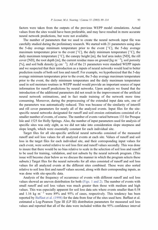
Analysis of the frequency of occurrence of events with different runoff and soil loss

values showed an uneven distribution for both (Figs. 1 and 2). The number of events with

small runoff and soil loss values was much greater then those with medium and high

values. This was especially apparent for soil loss data sets where events smaller than 0.58

and 1.16 kg m� 2 were 89% and 95% of cases, respectively. This tendency has been

reported by Baffaut et al. (1998) for the data from four of the sites used here. Baffaut et al.

estimated a Log-Pearson Type III (LP III) distribution parameters for measured soil loss

values and reported that all of the data were included within the 95% confidence interval


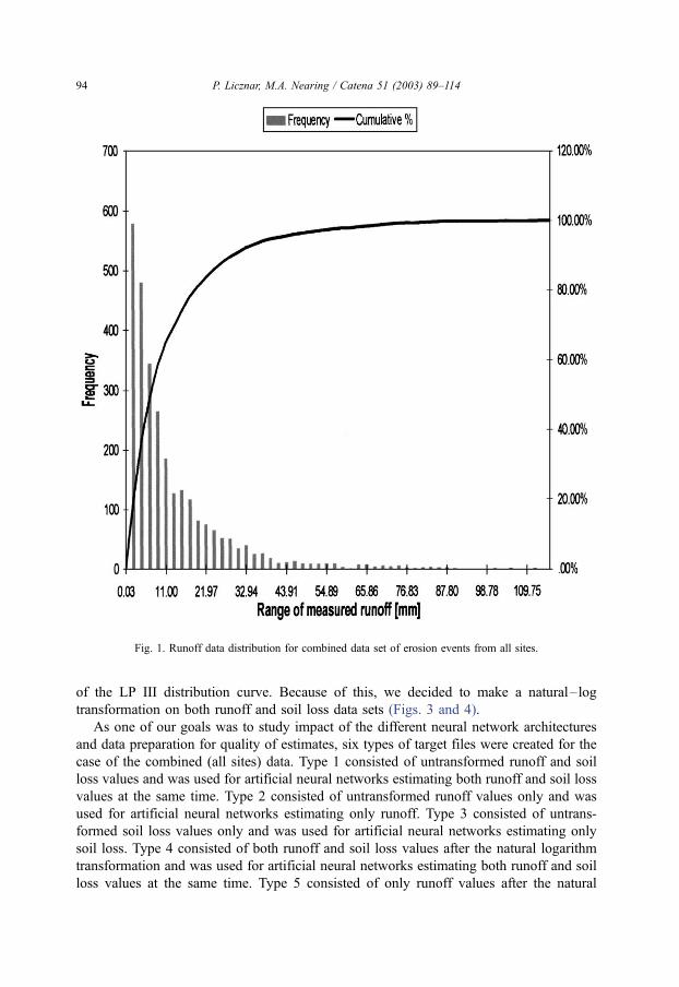
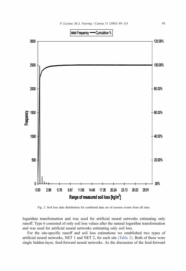
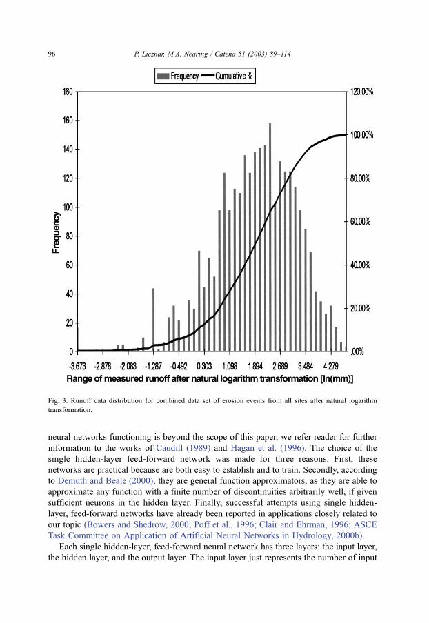
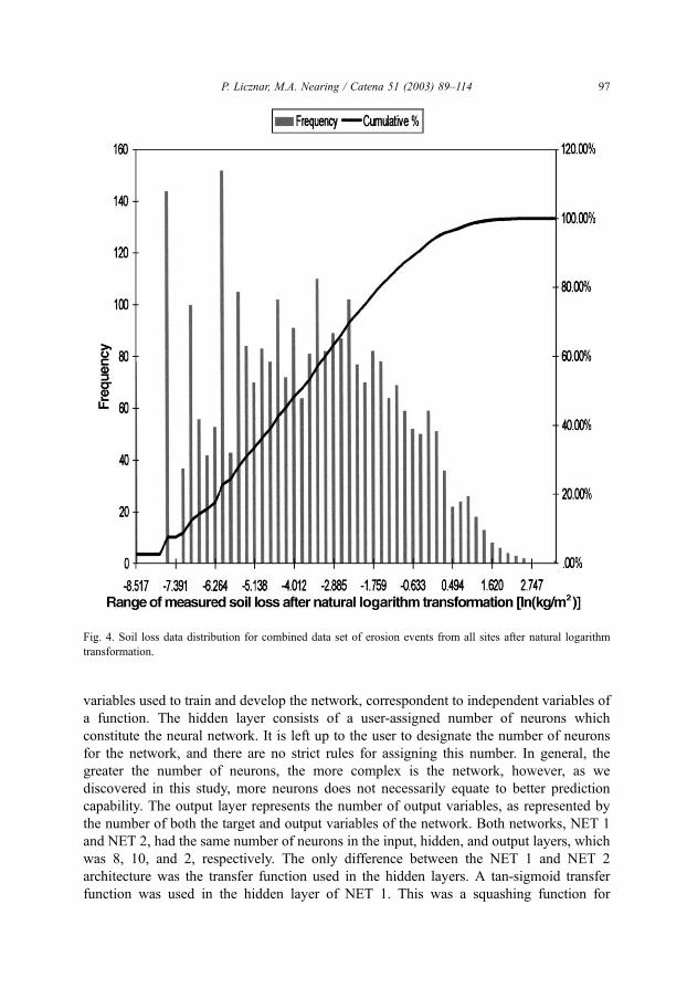
of the LP III distribution curve. Because of this, we decided to make a natural–log

transformation on both runoff and soil loss data sets (Figs. 3 and 4).

As one of our goals was to study impact of the different neural network architectures

and data preparation for quality of estimates, six types of target files were created for the

case of the combined (all sites) data. Type 1 consisted of untransformed runoff and soil

loss values and was used for artificial neural networks estimating both runoff and soil loss

values at the same time. Type 2 consisted of untransformed runoff values only and was

used for artificial neural networks estimating only runoff. Type 3 consisted of untrans-

formed soil loss values only and was used for artificial neural networks estimating only

soil loss. Type 4 consisted of both runoff and soil loss values after the natural logarithm

transformation and was used for artificial neural networks estimating both runoff and soil

loss values at the same time. Type 5 consisted of only runoff values after the natural

Fig. 1. Runoff data distribution for combined data set of erosion events from all sites.


logarithm transformation and was used for artificial neural networks estimating only

runoff. Type 6 consisted of only soil loss values after the natural logarithm transformation

and was used for artificial neural networks estimating only soil loss.

For the site-specific runoff and soil loss estimations we established two types of

artificial neural networks, NET 1 and NET 2, for each site (Table 2). Both of these were

single hidden-layer, feed-forward neural networks. As the discussion of the feed-forward

Fig. 2. Soil loss data distribution for combined data set of erosion events from all sites.


neural networks functioning is beyond the scope of this paper, we refer reader for further

information to the works of Caudill (1989) and Hagan et al. (1996). The choice of the

single hidden-layer feed-forward network was made for three reasons. First, these

networks are practical because are both easy to establish and to train. Secondly, according

to Demuth and Beale (2000), they are general function approximators, as they are able to

approximate any function with a finite number of discontinuities arbitrarily well, if given

sufficient neurons in the hidden layer. Finally, successful attempts using single hidden-

layer, feed-forward networks have already been reported in applications closely related to

our topic (Bowers and Shedrow, 2000; Poff et al., 1996; Clair and Ehrman, 1996; ASCE

Task Committee on Application of Artificial Neural Networks in Hydrology, 2000b).

Each single hidden-layer, feed-forward neural network has three layers: the input layer,

the hidden layer, and the output layer. The input layer just represents the number of input

Fig. 3. Runoff data distribution for combined data set of erosion events from all sites after natural logarithm

transformation.


variables used to train and develop the network, correspondent to independent variables of

a function. The hidden layer consists of a user-assigned number of neurons which

constitute the neural network. It is left up to the user to designate the number of neurons

for the network, and there are no strict rules for assigning this number. In general, the

greater the number of neurons, the more complex is the network, however, as we

discovered in this study, more neurons does not necessarily equate to better prediction

capability. The output layer represents the number of output variables, as represented by

the number of both the target and output variables of the network. Both networks, NET 1

and NET 2, had the same number of neurons in the input, hidden, and output layers, which

was 8, 10, and 2, respectively. The only difference between the NET 1 and NET 2

architecture was the transfer function used in the hidden layers. A tan-sigmoid transfer

function was used in the hidden layer of NET 1. This was a squashing function for

Fig. 4. Soil loss data distribution for combined data set of erosion events from all sites after natural logarithm

transformation.


mapping the input to the interval (� 1, 1) of the following form (Demuth and Beale,

2000):

f ðnÞ ¼ 1� e�n

1þ e�nð1Þ

A log-sigmoid transfer function was used in the hidden layer of NET 2. This was

squashing function for mapping the input to the interval (0, 1) of the following form

(Demuth and Beale, 2000):

f ðnÞ ¼ 1

1þ e�nð2Þ

Both networks’ output layer used a simple linear transfer function.

For estimation of runoff and soil loss values from the combined data (from all sites), 12

additional types of artificial neural networks were designated as NET 3 through NET 14

(Table 2). Each of them, as with the previously described NET 1 and NET 2, was a single

hidden-layer, feed-forward neural networks. A tan-sigmoid transfer function was used in

the hidden layer of NET 3 through NET 8, whereas a log-sigmoid transfer function was

used in the hidden layer of NET 9 through NET 14. A linear function was used as an

output layer transfer function for all the networks. The number of the neurons in the output

layer was equal to 2 for NET 3 and NET 9, as they were designated to be use with target

files of Type 1 (untransformed) that had both runoff and soil loss, and for NET 6 and NET

12, as they were designated to be use with target files of Type 4 (log-transformed) that had

both runoff and soil loss. The remanding eight networks had only one neuron in the output

layer as they were designated to be use with either runoff alone or soil loss alone. NET 4

and NET 10 were used with target files of Type 3 (untransformed for soil loss), NET 5 and

Table 2

Description of the 14 types of neural networks studied

NET Data set Transfer function type Target file type

1 Individual Sites Tan-Sigmoid 1 Untransformed, Both Variables

2 Individual Sites Log-Sigmoid 1 Untransformed, Both Variables

3 Combined Sites Tan-Sigmoid 1 Untransformed, Both Variables

4 Combined Sites Tan-Sigmoid 3 Untransformed, Soil Loss only

5 Combined Sites Tan-Sigmoid 2 Untransformed, Runoff only

6 Combined Sites Tan-Sigmoid 4 Log-Transformed, Both Variables

7 Combined Sites Tan-Sigmoid 6 Log-Transformed, Soil Loss only

8 Combined Sites Tan-Sigmoid 5 Log-Transformed, Runoff only

9 Combined Sites Log-Sigmoid 1 Untransformed, Both Variables

10 Combined Sites Log-Sigmoid 3 Untransformed, Soil Loss only

11 Combined Sites Log-Sigmoid 2 Untransformed, Runoff only

12 Combined Sites Log-Sigmoid 4 Log-Transformed, Both Variables

13 Combined Sites Log-Sigmoid 6 Log-Transformed, Soil Loss only

14 Combined Sites Log-Sigmoid 5 Log-Transformed, Runoff only

NET 1 and NET 2 used eight input parameters and 10 hidden layers within the network. NET 3 through NET 14

used 10 input parameters, and each of these nets were developed five times using 10, 20, 30, 40, and 50 hidden

layers.


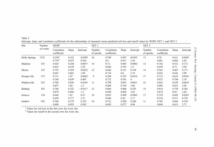
Table 3

Intercept, slope, and correlation coefficients for the relationships of measured versus predicted soil loss and runoff values by WEPP, NET 1, and NET 2

Site Number WEPP NET 1 NET 2

of eventsCorrelation

coefficient

Slope Intercept Number

of epochs

Correlation

coefficient


of epochs

Correlation

coefficient

Slope Intercept

Holly Springs 1525 0.238a 0.162 0.0389 24 0.789 0.697 0.0345 13 0.76 0.611 0.0487

0.735b 0.675 0.934 0.9 0.817 2.54 0.891 0.805 2.65

Madison 143 0.624 0.244 0.0837 14 0.72 0.603 0.0882 12 0.762 0.512 0.172

0.823 0.678 2.29 0.896 0.791 1.9 0.859 0.73 2.09

Morris 147 0.753 0.369 0.0252 12 0.666 0.511 0.194 14 0.563 0.467 0.171

0.647 0.801 1.09 0.714 0.6 2.74 0.643 0.641 2.09

Presque Isle 133 0.711 1.07 0.0682 9 0.584 0.355 0.0516 17 0.712 0.619 0.0541

0.768 0.659 0.407 0.752 0.561 4 0.837 0.704 2.19

Watkinsville 252 0.768 0.856 0.0165 11 0.798 0.691 0.0811 23 0.842 0.839 0.0625

0.857 1.02 1.2 0.884 0.745 3.04 0.903 0.815 2.05

Bethany 383 0.768 0.332 � 0.0117 12 0.866 0.806 0.293 14 0.814 0.754 0.205

0.879 0.866 1.3 0.894 0.802 3.83 0.874 0.85 2.44

Geneva 134 0.664 1.01 0.21 14 0.693 0.499 0.0945 17 0.738 0.685 0.0267

0.638 0.717 3.11 0.686 0.56 2.17 0.514 0.511 0.745

Guthrie 292 0.766 0.279 0.235 10 0.512 0.209 0.286 11 0.702 0.464 0.328

0.889 0.955 0.582 0.693 0.577 8.08 0.896 0.813 2.77

a Values for soil loss in the first rows for every site.b Values for runoff in the second rows for every site.

P.Liczn

ar,M.A.Nearin

g/Caten

a51(2003)89–114

99

NET 11 with target files of Type 2 (untransformed for runoff), NET 7 and NET 13 with

target files of Type 6 (log-transformed for soil loss), NET 8 and NET 14 with target files of

Type 5 (log-transformed for runoff). In each case for NET 3 through NET 14, a different

net was developed using the number of the neurons in the hidden layer of 10, 20, 30, 40 or

50 in order to evaluate the influence of number of internal neurons on the precision of the

network estimates.

The Levenberg–Marquardt algorithm was chosen for training of all networks. This

algorithm belongs to the group of quasi-Newton algorithms allowing rapid training, but, as

opposed to the Newton method, it does not require a Hessian matrix of the performance

index at the current values of the weights and biases to be computed. This makes it less

complicated and memory demanding, which is why it is often used in artificial network

training and was chosen also for the purpose of this study. A more detailed description of

Levenberg–Marquardt algorithm may be found in Hagan et al. (1996).

Usually, neural networks are more efficient if certain preprocessing steps are made

(Demuth and Beale, 2000). Because of this, all the input and output were scaled so that

they had zero means and unity standard deviation. After every simulation, network outputs

were converted in the post-processing step back to the original units. Also, a principal

component analysis was applied in order to eliminate the components that contribute the

least to the variation of data. This specific technique had three effects (Demuth and Beale,

2000): it orthogonalized the components of the input vectors, so that they were

uncorrelated with one another, it ordered the resulting orthogonal components so that

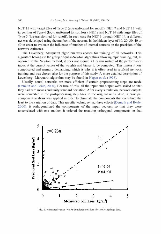
Fig. 5. Measured versus WEPP predicted soil loss for Holly Springs data.


those with the largest variation came first, and it eliminated those components that

contributed the least to the variation in the data set. Those principal components that

accounted for 99.9% of the variation in the data sets were retained. The results of this

technique led to the discovery of the observation reported above of similarity of interrill

and rill cover parameters for most of analyzed events.

After preprocessing the input and target sets, the data were divided into three subsets:

the training subset (50% of the total), the validation subset (25% of the total), and the test

subset (25% of all set). The test subset was comprised of every fourth record beginning

with the second record and the validation subset set was comprised of every fourth record

beginning with the fourth record. All other records were put into training subset. This

operation was made in connection with above described sorting of runoff and soil loss

values (and corresponding inputs) in the target files. Dividing of the data into three subsets

was mandatory, since the ‘‘early stopping’’ method for improving the generalization of the

networks was implemented. In this method, error on the validation subset is monitored

during the training process. It usually decreases at the beginning of training, as does the

error of training subset. At some point during the training it is common that the network

begins to overfit the data, and then the validation error begins to rise. When the validation

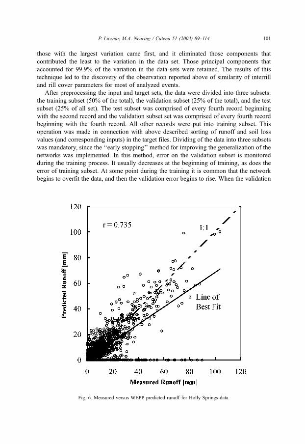
Fig. 6. Measured versus WEPP predicted runoff for Holly Springs data.


error increases for a number of iterations, the training is terminated and the weights and

biases at the minimum of the validation error are assumed as optimum (Demuth and Beale,

2000). Over-fitting is undesirable, since the goal of the network training was not to mimic

the training data themselves (including the noise in the training data) but to learn the

underlying system that generated the training data.

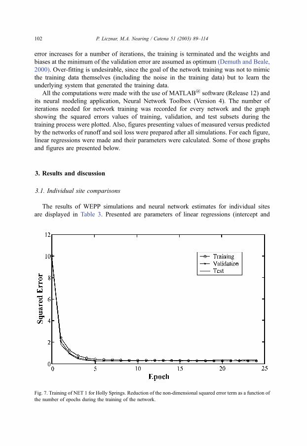
All the computations were made with the use of MATLAB@ software (Release 12) and

its neural modeling application, Neural Network Toolbox (Version 4). The number of

iterations needed for network training was recorded for every network and the graph

showing the squared errors values of training, validation, and test subsets during the

training process were plotted. Also, figures presenting values of measured versus predicted

by the networks of runoff and soil loss were prepared after all simulations. For each figure,

linear regressions were made and their parameters were calculated. Some of those graphs

and figures are presented below.

3. Results and discussion

3.1. Individual site comparisons

The results of WEPP simulations and neural network estimates for individual sites

are displayed in Table 3. Presented are parameters of linear regressions (intercept and

Fig. 7. Training of NET 1 for Holly Springs. Reduction of the non-dimensional squared error term as a function of

the number of epochs during the training of the network.


slope of the best fit lines and correlation coefficients) for relationships between

measured and predicted runoff and soil loss by the WEPP model and networks NET

1 and NET 2. Information regarding the number of epochs training lasted for NET 1

and NET 2 is also supplied in Table 3. The number of epochs refers to the number of

computational cycles used by the neural network software in arriving at the optimal

network parameters.

The WEPP model predicted better for runoff than for soil loss for nearly all sites. The

difference was especially apparent for the Holly Springs site (see Figs. 5 and 6) where

runoff was predicted reasonably well (the correlation coefficient and a slope of best fit line

were equal to 0.735 and 0.675, respectively), whereas soil loss was predicted poorly (the

correlation coefficient was 0.238). The reverse tendency for WEPP of predicting better soil

loss than runoff was observed only in cases of Geneva and Morris. However, for the

Morris site, while the correlation coefficient was high, the slope and intercept values of the

best-fit line for soil loss were quite low, which suggests a strong tendency to underpredict

large events by WEPP for that site. The WEPP model at the Geneva site had very precise

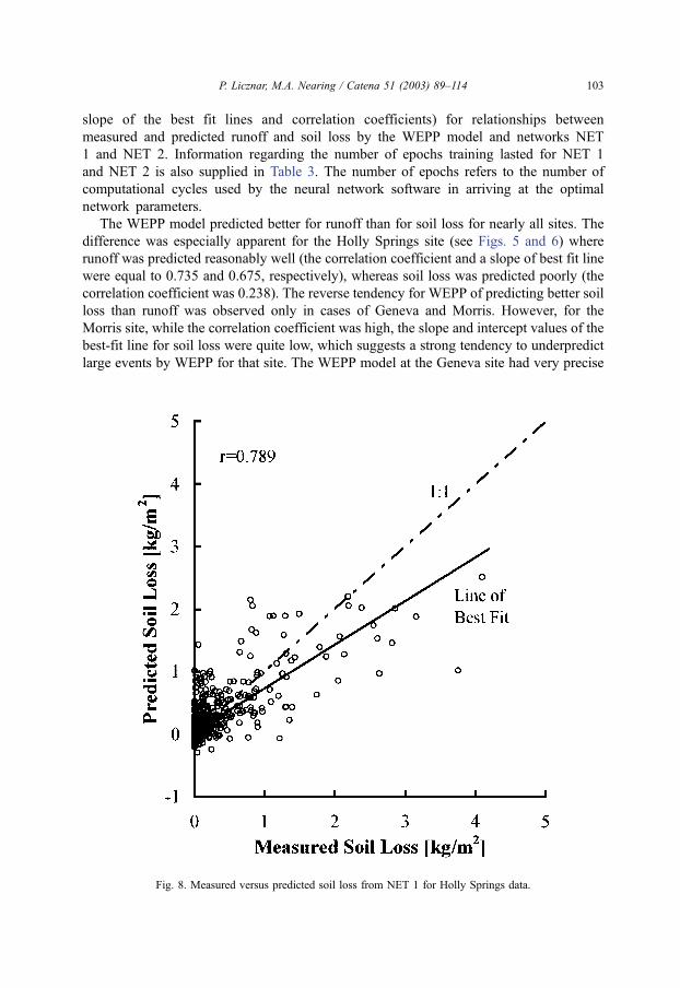
Fig. 8. Measured versus predicted soil loss from NET 1 for Holly Springs data.


soil loss estimates, with slope and intercept values equal to 1.01 and 0.21, respectively,

suggesting that the trend line was close to the 1:1 slope line. For all the sites except

Presque Isle, Watkinsville and Geneva, slope values of the best-fit lines for soil loss were

less than the best-fit slope values for runoff. This observed trend of predicting better runoff

than soil loss was in agreement with previous results of WEPP model performance studies

at the plot scale by Zhang et al. (1996) and with general conclusions considering modeling

of soil erosion by water of Boardman and Favis-Mortlock (1998). Slope values for soil

loss and runoff best fit lines for nearly all cases were less than 1 and intercept values were

usually greater than 0. This result highlights the tendency for erosion models in general,

and WEPP in particular, to under-predict large events and over-predict small events, which

has been discussed in detail by Nearing (1998).

NET 1 and NET 2 simulations gave encouraging results. Results obtained from at least

one of the two networks for most of the sites were better than the results from WEPP. That

was true for both soil loss and runoff estimates. Only for Morris, Presque Isle and Guthrie

sites were results from neural networks simulations approximately of the same or slightly

lower quality as the results received from WEPP. It is worth noting that all those three sites

had a relatively smaller number of events, which may have made the training subset of

data too small for an optimal training of the network. This may be also shown to some

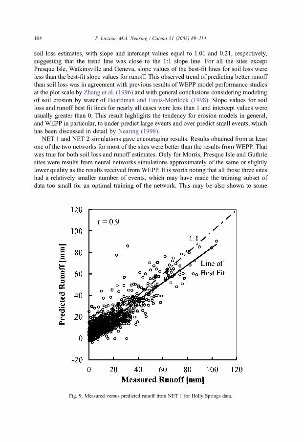
Fig. 9. Measured versus predicted runoff from NET 1 for Holly Springs data.


extend by the fact that the number of epochs needed for training of those site-specific

networks was relatively small. At Presque Isle NET 2 was trained for eight epochs longer

than was NET 1, and resultant performance of the network was improved. Soil loss and

runoff correlation coefficient values increased from 0.584 and 0.752 to 0.712 and 0.837,

respectively; regression line slope values increased from 0.355 and 0.561 to 0.619 and

0.704, respectively; and intercept values were the same or slightly less. In general,

however, no great differences were observed between the quality of outputs from NET 1

and NET 2 for the different sites. It seems that the improved results from one of the

networks, as it was in the case of Presque Isle, may not be attributed to the specific

activation function used in the hidden layer but to the longer training process. For

example, for the Holly Spring site, NET 1, which trained during 24 epochs (see Fig. 7),

provided better estimates than did NET 2, which trained during only 13 epochs. Likewise,

the Watkinsville site NET 2, which trained during 23 epochs, gave better results than NET

1, which trained during 11 epochs.

Particularly better predictions for both networks in comparison to WEPP results were

found for Holly Springs. This was especially true for soil loss, where the correlation

coefficient and slope of best-fit line increased by a factor of approximately three to a

value of 0.789 and 0.697, respectively, for NET 1 (Fig. 8). For runoff, the correlation

coefficient and slope of best-fit line increased to the value of 0.9 and 0.817, respectively,

for NET 1 (Fig. 9). We presume that the positive results for networks for Holly Springs

were because this was the site with the largest data set, with a total number of 1525

events. This allowed the preparation of very good training and validation subsets.

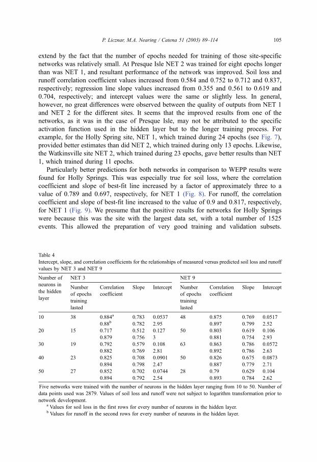
Table 4

Intercept, slope, and correlation coefficients for the relationships of measured versus predicted soil loss and runoff

values by NET 3 and NET 9

Number of NET 3 NET 9

neurons in

the hidden

layer

Number

of epochs

training

lasted

Correlation

coefficient


of epochs

training

lasted

Correlation

coefficient

Slope Intercept

10 38 0.884a 0.783 0.0537 48 0.875 0.769 0.0517

0.88b 0.782 2.95 0.897 0.799 2.52

20 15 0.717 0.512 0.127 50 0.803 0.619 0.106

0.879 0.756 3 0.881 0.754 2.93

30 19 0.792 0.579 0.108 63 0.863 0.786 0.0572

0.882 0.769 2.81 0.892 0.786 2.63

40 23 0.825 0.708 0.0901 50 0.826 0.675 0.0873

0.894 0.798 2.47 0.887 0.779 2.71

50 27 0.852 0.702 0.0744 28 0.79 0.629 0.104

0.894 0.792 2.54 0.893 0.784 2.62

Five networks were trained with the number of neurons in the hidden layer ranging from 10 to 50. Number of

data points used was 2879. Values of soil loss and runoff were not subject to logarithm transformation prior to

network development.a Values for soil loss in the first rows for every number of neurons in the hidden layer.b Values for runoff in the second rows for every number of neurons in the hidden layer.


However, detailed analysis of the neural network predicted soil loss and runoff showed

anomalies in the predictions. It was observed that in the case of some small events neural

networks predictions yielded negative values of soil loss and runoff (see Figs. 8 and 9).

Since neural networks functioned as black box models they estimated abnormal

(negative) values of soil loss and runoff, which was not the case for the physically

based WEPP model predictions.

Networks NET 1 and NET 2 generally displayed better abilities of runoff than of soil

loss estimation. The only exception was for Geneva. The tendency to under-predict large

events and over-predict small ones for all the site-specific networks NET 1 and NET 2 was

qualitatively similar with the results reported above for the WEPP predictions.

3.2. Combined data comparisons

The summary comparisons of the WEPP predicted soil loss and runoff values versus

measured for all site data combined yielded the following results: for soil loss the

correlation coefficient was equal to 0.621 and the slope and the intercept of the best fit

line were 0.335 and 0.08; for runoff the correlation coefficient was equal to 0.603 and the

slope and the intercept of the best fit line were 0.759 and 1.138. As it was in the case of

NET 1 and NET 2, training of all networks of type NET 3 through NET 14 was

successfully accomplished and terminated by validation stop. All the parameters of linear

regressions (intercepts, slopes, and correlation coefficients) for relationships between

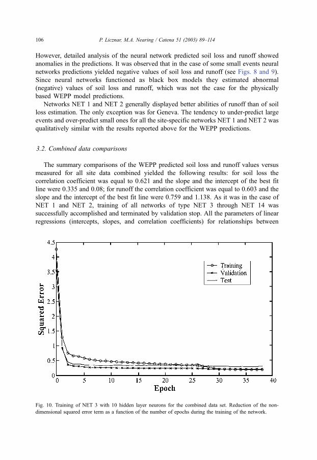
Fig. 10. Training of NET 3 with 10 hidden layer neurons for the combined data set. Reduction of the non-

dimensional squared error term as a function of the number of epochs during the training of the network.


measured and predicted both soil loss and runoff values for networks NET 3 through NET

14, and for the different number of neurons in the hidden layer, are presented in Tables 4–

9. Also, results of the training process and relations of predicted versus measured values

are presented for NET 3 with 10 neurons in the hidden layer in Figs. 10–12, and for NET

13 with 50 neurons in the hidden layer in Figs. 13 and 14.

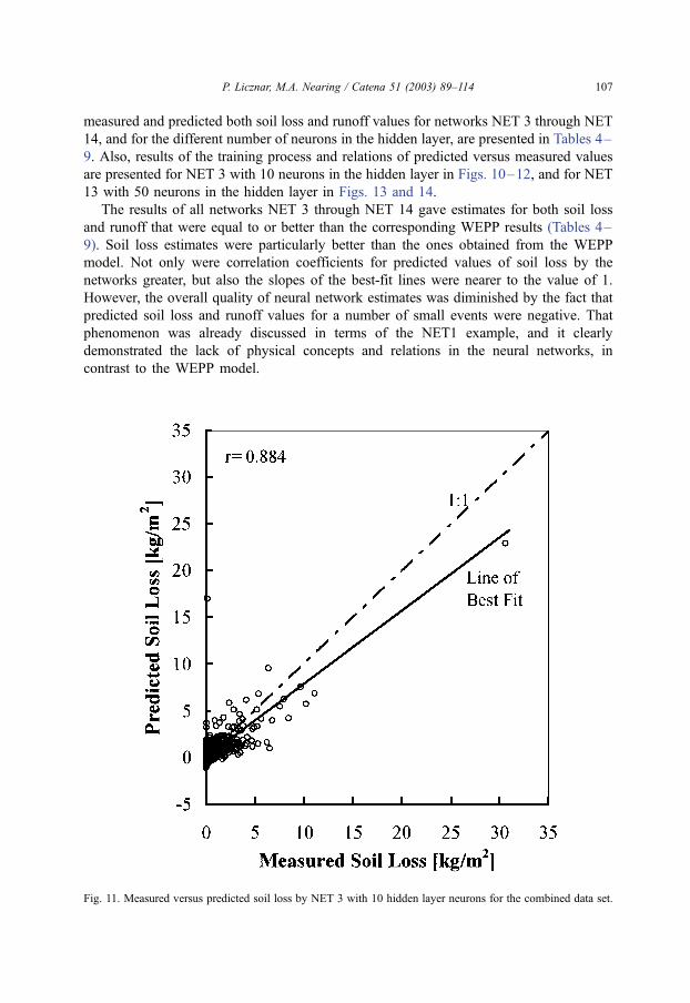
The results of all networks NET 3 through NET 14 gave estimates for both soil loss

and runoff that were equal to or better than the corresponding WEPP results (Tables 4–

9). Soil loss estimates were particularly better than the ones obtained from the WEPP

model. Not only were correlation coefficients for predicted values of soil loss by the

networks greater, but also the slopes of the best-fit lines were nearer to the value of 1.

However, the overall quality of neural network estimates was diminished by the fact that

predicted soil loss and runoff values for a number of small events were negative. That

phenomenon was already discussed in terms of the NET1 example, and it clearly

demonstrated the lack of physical concepts and relations in the neural networks, in

contrast to the WEPP model.

Fig. 11. Measured versus predicted soil loss by NET 3 with 10 hidden layer neurons for the combined data set.


We were not able with these results to identify a single best architecture for the runoff

and soil loss estimates. It was found that the activation function used in the hidden layer

did not strongly influence the quality of results. Results from NET 3 for each analyzed

number of hidden layer neurons were quite similar to the NET 9 results (Table 4). The

same was observed for the other pairs of networks: NET 4 and NET 10, NET 5 and NET

11, NET 6 and NET 12, NET 7 and NET 13, and NET 8 and NET 14 (Tables 5–9). Also,

the optimal number of neurons in the hidden layer was not established in these results. The

increase in the number of hidden layer neurons did not generally yield better network

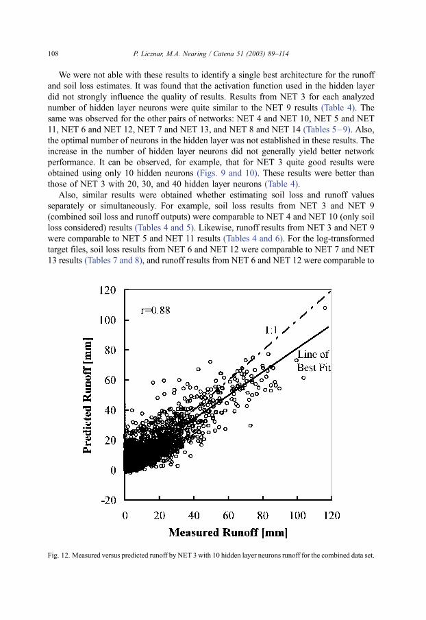
performance. It can be observed, for example, that for NET 3 quite good results were

obtained using only 10 hidden neurons (Figs. 9 and 10). These results were better than

those of NET 3 with 20, 30, and 40 hidden layer neurons (Table 4).

Also, similar results were obtained whether estimating soil loss and runoff values

separately or simultaneously. For example, soil loss results from NET 3 and NET 9

(combined soil loss and runoff outputs) were comparable to NET 4 and NET 10 (only soil

loss considered) results (Tables 4 and 5). Likewise, runoff results from NET 3 and NET 9

were comparable to NET 5 and NET 11 results (Tables 4 and 6). For the log-transformed

target files, soil loss results from NET 6 and NET 12 were comparable to NET 7 and NET

13 results (Tables 7 and 8), and runoff results from NET 6 and NET 12 were comparable to

Fig. 12. Measured versus predicted runoff by NET 3 with 10 hidden layer neurons runoff for the combined data set.


NET 8 and NET 14 results (Tables 7 and 9). Constructing the neural network on the

individual output parameters rather than the two outputs at the same time did not improve

the prediction capability of the resultant network.

On the other hand, the preparation process of log-transforming the target files did

appear to influence the quality of neural network estimates. Comparison of NET 4 and

NET 10 performances with NET 7 and NET 13 performances allowed us to conclude that

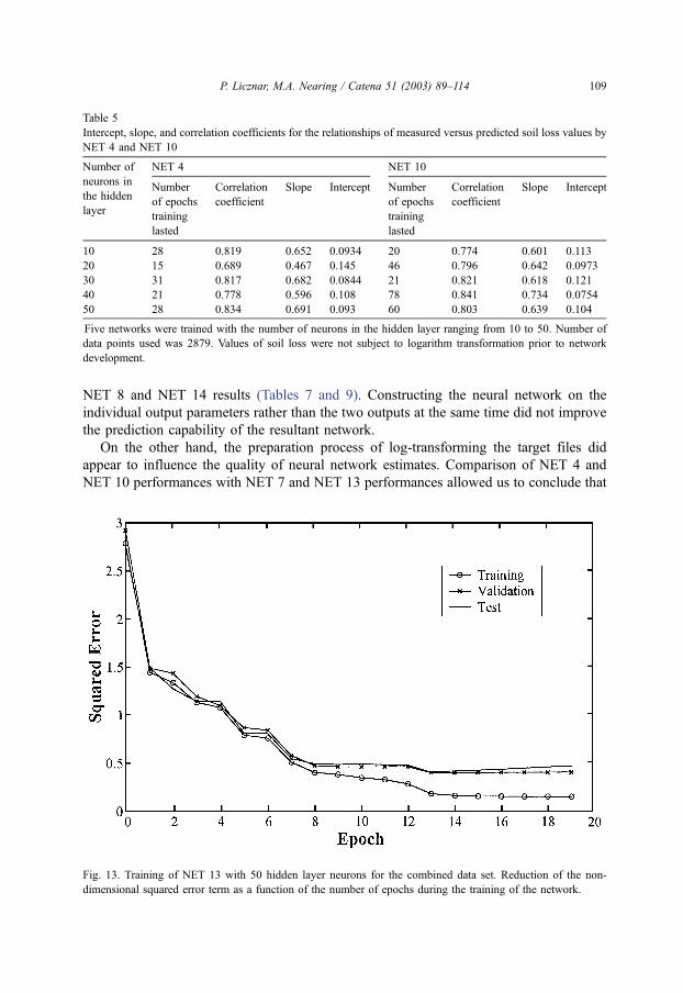
Fig. 13. Training of NET 13 with 50 hidden layer neurons for the combined data set. Reduction of the non-

dimensional squared error term as a function of the number of epochs during the training of the network.

Table 5

Intercept, slope, and correlation coefficients for the relationships of measured versus predicted soil loss values by

NET 4 and NET 10


neurons in

the hidden

layer

Number

of epochs

training

lasted

Correlation

coefficient


of epochs

training

lasted

Correlation

coefficient

Slope Intercept

10 28 0.819 0.652 0.0934 20 0.774 0.601 0.113

20 15 0.689 0.467 0.145 46 0.796 0.642 0.0973

30 31 0.817 0.682 0.0844 21 0.821 0.618 0.121

40 21 0.778 0.596 0.108 78 0.841 0.734 0.0754

50 28 0.834 0.691 0.093 60 0.803 0.639 0.104


data points used was 2879. Values of soil loss were not subject to logarithm transformation prior to network

development.


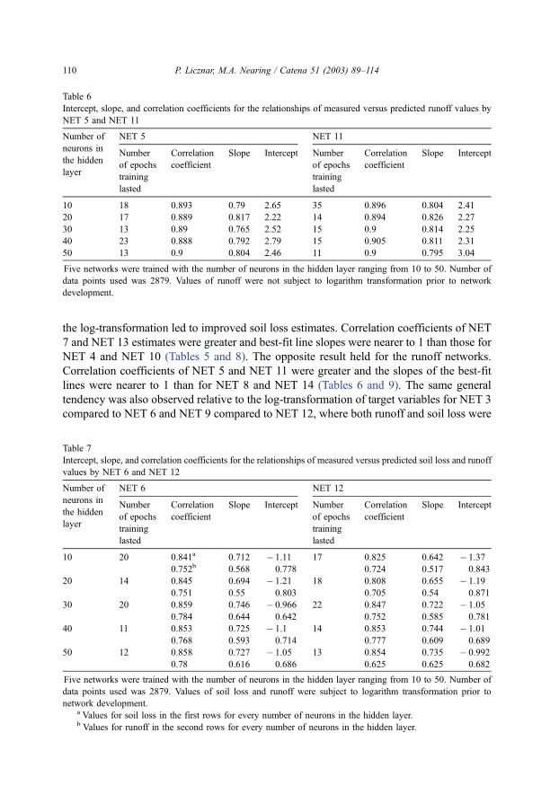
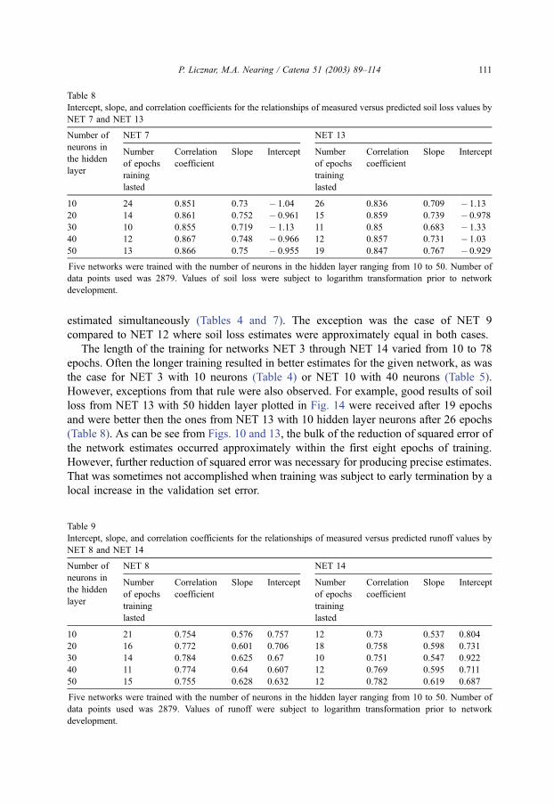
the log-transformation led to improved soil loss estimates. Correlation coefficients of NET

7 and NET 13 estimates were greater and best-fit line slopes were nearer to 1 than those for

NET 4 and NET 10 (Tables 5 and 8). The opposite result held for the runoff networks.

Correlation coefficients of NET 5 and NET 11 were greater and the slopes of the best-fit

lines were nearer to 1 than for NET 8 and NET 14 (Tables 6 and 9). The same general

tendency was also observed relative to the log-transformation of target variables for NET 3

compared to NET 6 and NET 9 compared to NET 12, where both runoff and soil loss were

Table 6

Intercept, slope, and correlation coefficients for the relationships of measured versus predicted runoff values by

NET 5 and NET 11


neurons in

the hidden

layer

Number

of epochs

training

lasted

Correlation

coefficient


of epochs

training

lasted

Correlation

coefficient

Slope Intercept

10 18 0.893 0.79 2.65 35 0.896 0.804 2.41

20 17 0.889 0.817 2.22 14 0.894 0.826 2.27

30 13 0.89 0.765 2.52 15 0.9 0.814 2.25

40 23 0.888 0.792 2.79 15 0.905 0.811 2.31

50 13 0.9 0.804 2.46 11 0.9 0.795 3.04


data points used was 2879. Values of runoff were not subject to logarithm transformation prior to network

development.

Table 7

Intercept, slope, and correlation coefficients for the relationships of measured versus predicted soil loss and runoff

values by NET 6 and NET 12


neurons in

the hidden

layer

Number

of epochs

training

lasted

Correlation

coefficient


of epochs

training

lasted

Correlation

coefficient

Slope Intercept

10 20 0.841a 0.712 � 1.11 17 0.825 0.642 � 1.37

0.752b 0.568 0.778 0.724 0.517 0.843

20 14 0.845 0.694 � 1.21 18 0.808 0.655 � 1.19

0.751 0.55 0.803 0.705 0.54 0.871

30 20 0.859 0.746 � 0.966 22 0.847 0.722 � 1.05

0.784 0.644 0.642 0.752 0.585 0.781

40 11 0.853 0.725 � 1.1 14 0.853 0.744 � 1.01

0.768 0.593 0.714 0.777 0.609 0.689

50 12 0.858 0.727 � 1.05 13 0.854 0.735 � 0.992

0.78 0.616 0.686 0.625 0.625 0.682


data points used was 2879. Values of soil loss and runoff were subject to logarithm transformation prior to

network development.a Values for soil loss in the first rows for every number of neurons in the hidden layer.b Values for runoff in the second rows for every number of neurons in the hidden layer.


estimated simultaneously (Tables 4 and 7). The exception was the case of NET 9

compared to NET 12 where soil loss estimates were approximately equal in both cases.

The length of the training for networks NET 3 through NET 14 varied from 10 to 78

epochs. Often the longer training resulted in better estimates for the given network, as was

the case for NET 3 with 10 neurons (Table 4) or NET 10 with 40 neurons (Table 5).

However, exceptions from that rule were also observed. For example, good results of soil

loss from NET 13 with 50 hidden layer plotted in Fig. 14 were received after 19 epochs

and were better then the ones from NET 13 with 10 hidden layer neurons after 26 epochs

(Table 8). As can be see from Figs. 10 and 13, the bulk of the reduction of squared error of

the network estimates occurred approximately within the first eight epochs of training.

However, further reduction of squared error was necessary for producing precise estimates.

That was sometimes not accomplished when training was subject to early termination by a

local increase in the validation set error.

Table 8

Intercept, slope, and correlation coefficients for the relationships of measured versus predicted soil loss values by

NET 7 and NET 13


neurons in

the hidden

layer

Number

of epochs

raining

lasted

Correlation

coefficient


of epochs

training

lasted

Correlation

coefficient

Slope Intercept

10 24 0.851 0.73 � 1.04 26 0.836 0.709 � 1.13

20 14 0.861 0.752 � 0.961 15 0.859 0.739 � 0.978

30 10 0.855 0.719 � 1.13 11 0.85 0.683 � 1.33

40 12 0.867 0.748 � 0.966 12 0.857 0.731 � 1.03

50 13 0.866 0.75 � 0.955 19 0.847 0.767 � 0.929


data points used was 2879. Values of soil loss were subject to logarithm transformation prior to network

development.

Table 9

Intercept, slope, and correlation coefficients for the relationships of measured versus predicted runoff values by

NET 8 and NET 14


neurons in

the hidden

layer

Number

of epochs

training

lasted

Correlation

coefficient


of epochs

training

lasted

Correlation

coefficient

Slope Intercept

10 21 0.754 0.576 0.757 12 0.73 0.537 0.804

20 16 0.772 0.601 0.706 18 0.758 0.598 0.731

30 14 0.784 0.625 0.67 10 0.751 0.547 0.922

40 11 0.774 0.64 0.607 12 0.769 0.595 0.711

50 15 0.755 0.628 0.632 12 0.782 0.619 0.687


data points used was 2879. Values of runoff were subject to logarithm transformation prior to network

development.


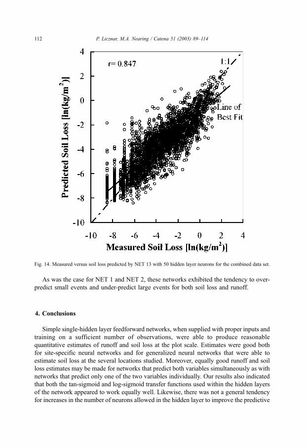
As was the case for NET 1 and NET 2, these networks exhibited the tendency to over-

predict small events and under-predict large events for both soil loss and runoff.

4. Conclusions

Simple single-hidden layer feedforward networks, when supplied with proper inputs and

training on a sufficient number of observations, were able to produce reasonable

quantitative estimates of runoff and soil loss at the plot scale. Estimates were good both

for site-specific neural networks and for generalized neural networks that were able to

estimate soil loss at the several locations studied. Moreover, equally good runoff and soil

loss estimates may be made for networks that predict both variables simultaneously as with

networks that predict only one of the two variables individually. Our results also indicated

that both the tan-sigmoid and log-sigmoid transfer functions used within the hidden layers

of the network appeared to work equally well. Likewise, there was not a general tendency

for increases in the number of neurons allowed in the hidden layer to improve the predictive

Fig. 14. Measured versus soil loss predicted by NET 13 with 50 hidden layer neurons for the combined data set.


capabilities of the network. The ability of the network to provide good predictions of soil

loss improved when the target and output values of soil loss were transformed to natural

logarithms of the soil loss values. This was not true for runoff estimates, in which case the

untransformed target values produced better network predictions.

Performances of neural networks were as good as or better than the performance of the

WEPP model, which belongs to the class of new, physically based erosion prediction

technologies. Since the amount of information that must be introduced to a physically based

model is extensive in comparison with the artificial network demands, the neural networks

can be seen as a future supplementary or sometimes complementary tool in erosion

prediction technology. However, our study results show clearly that neural networks have

also a number of disadvantages that should be seriously considered prior their application.

First of all, the success of neural network application depends and is completely determined

by the quality and quantity of available data. In the erosion prediction practice that

requirement usually is not easily met. Requisite data very often are not available and have to

be generated by other means, for example by use of a complex physically based model.

That was the case in this study wherein some of the neural networks inputs were generated

by the physically based WEPP model. Another major limitation in widespread use of neural

networks is the lack of physical concepts and relations. That may lead to abnormal

(physically nonsensical) prediction results and certainly does not allow us for better

understanding of the complex functioning of the erosional system. This factor has important

implications for extending the application of the model to new environments.

Before using neural networks for a particular erosion prediction application, research

should be done to establish the best input parameters for network performances and to

optimize their architectures. Such optimization is not easy since there is no one stand-

ardized procedure of selecting network architecture and it may also vary depending upon

the environment to which neural networks are applied. It is reasonable to assume that

erosion on construction sites or in forests, for example, may lead to a very different set of

optimum parameters and network architecture than those presented here.

Acknowledgements

We wish to thank the Polish–U.S. Fulbright Commission for supporting Pawel Licznar

with funds for a 5-month stay at the Purdue University, which gave him unique opportunity

to extend his interest in the field of soil erosion and neural networks. We also would like to

appreciate courtesy of the Stephan Batory Foundation, which covered all the costs of Pawel

Licznar’s scholarship at the University of Bologna. That program greatly enhanced his

knowledge of soil erosion research and stimulated his interest in neural networks.

References

ASCE Task Committee on Application of Artificial Neural Networks in Hydrology, 2000a. Artificial neural

networks in hydrology: I. Preliminary concepts. Journal of Hydrologic Engineering 5 (2), 115–123.

ASCE Task Committee on Application of Artificial Neural Networks in Hydrology, 2000b. Artificial neural

networks in hydrology: II. Hydrologic applications. Journal of Hydrologic Engineering 5 (2), 124–137.


Ascough III, J.C., Baffaut, C., Nearing, M.A., Liu, B.Y., 1997. The WEPP watershed model: I. Hydrology and

erosion. Transactions of the ASAE 40 (4), 921–933.

Baffaut, C., Nearing, M.A., Govers, G., 1998. Statistical distribution of soil loss from runoff plots and WEPP

model simulations. Soil Science Society of America Journal 62 (3), 756–763 (May–June).

Boardman, J., Favis-Mortlock, D., 1998. Modeling soil erosion by water: some conclusions. Modeling Soil

Erosion by Water. NATO ASI Series I, vol. 55. Springer-Verlag, Berlin, pp. 515–517.

Bowers, J.A., Shedrow, C.B., 2000. Predicting stream water quality using artificial neural networks. U.S. Depart-

ment of Energy Report WSRC-MS-2000-00112, 7 pp.

Caudill, M., 1989. Neural Network Primer. Miller Freeman Publications, San Francisco, CA.

Clair, T.A., Ehrman, J.M., 1996. Limnology and Oceanography 41 (5), 921–927.

Demuth, H., Beale, M., 2000. Neural Network Toolbox for Use with MATLAB, Users Guide Version 4. The

Math Works, Natic, ME.

Hagan, M.T., Demuth, H.B., Beale, M.H., 1996. Neural Network Design. PWS Publishing, Boston, MA.

Harris, T.M., Boardman, J., 1998. Alternative approaches to soil erosion prediction and conservation using expert

systems and neural networks. Modeling Soil Erosion by Water. NATO ASI Series I, vol. 55. Springer-Verlag,

Berlin, pp. 461–477.

Hornik, K., 1991. Approximation capabilities of multilayer feedforward networks. Neural Networks 4, 251–257.

Lane, L.J., Nearing, M.A., 1989. USDA-Water Erosion Prediction Project-Hillslope Profile Version. NSERL

Report No. 2. US Department of Agriculture, Agriculture Research Service, W. Lafayette, IN.

Nearing, M.A., 1998. Why soil erosion models over-predict small soil losses and under-predict large soil losses.

Catena 32, 15–22.

Nearing, M.A., Govers, G., Norton, D.L., 1999. Variability in soil erosion data from replicated plots. Soil Science

Society of America Journal 63 (6), 1829–1835 (November–December).

Poff, N.L., Tokar, S., Johnson, P., 1996. Limnology and Oceanography 41 (5), 857–863.

Renard, K.G., Foster, G.R., Weesies, G.A., Porter, P.J., 1991. RUSLE—revised universal soil loss equation.

Journal of Soil and Water Conservation, 30–33 (January–February).

Renard, K.G., Foster, G.R., Weesies, G.A., McCool, D.K., Yoder, D.C., 1996. Predicting Soil Erosion By Water:

A Guide to Conservation Planning with the Revised Universal Soil Loss Equation (RUSLE). Soil and Water

Conservation Society, Tucson, AZ. 383 pp.

Rosa, D., de la Mayol, F., Lozano, S., 1999. An expert system/neural network model (impelERO) for evaluating

agricultural soil erosion in Andalucia region, southern Spain. Agriculture, Ecosystems and Environment 73

(3), 211–226.

Wischmeier, W.H., Smith, D.D., 1958. Rainfall energy and its relationship to soil loss. Transactions-American

Geophysical Union 39 (2), 285–291.

Wischmeier, W.H., Smith, D.D., 1978. Predicting rainfall erosion losses: a guide to conservation planning. Agric.

Handbook No. 282. US Department of Agriculture, Washington, DC.

Zhang, X.C., Nearing, M.A., Risse, L.M., McGregor, K.C., 1996. Evaluation of WEPP runoff and soil loss

predictions using natural runoff plot data. Transactions of the ASAE 39 (3), 855–863.


Documents

Artificial neural networks of soil erosion and runoff prediction at the