Embed Size (px)
Citation preview
FULL DISSERTATION
Submitted in fulfilment of the requirements for the degree of MASTER OF SCIENCE in
the field of HYDROLOGY in the Faculty of Science and Agriculture at the University of
Zululand
With the title:
SIMULATION OF CATCHMENT RUNOFF, EROSION AND
SEDIMENT TRANSPORT USING A TRANSIENT
NUMERICAL MODEL FOR MLALAZI CATCHMENT
FACULTY OF SCIENCE AND AGRICULTURE
Candidate: Khathutshelo Joshua Rasifudi
Student number: 201454749
Supervisor: Prof J Simonis
Co-supervisor: Prof B Kelbe and Mr B K Rawlins
February 2019

S I MU L A TI O N O F C A TC H ME N T R U N O F F , E R OS I O N A N D S E DI ME N T TR A N S P O R T U S I N G A TR A N S I E N T N U ME R I C A L MO D E L F O R ML A L A Z I C A TC H ME N T
i
DEDICATION
This work can only be dedicated to the Lord, He is the Ultimate keeper. His love,
generosity and kindness are very fundamental and I thank Him for keeping me in the
high place of confidence and faith, hence this work a success.

S I MU L A TI O N O F C A TC H ME N T R U N O F F , E R OS I O N A N D S E DI ME N T TR A N S P O R T U S I N G A TR A N S I E N T N U ME R I C A L MO D E L F O R ML A L A Z I C A TC H ME N T
ii
DECLARATION
I Rasifudi Khathutshelo Joshua of student number 201454749 declare that this research
is my own work and is submitted in fulfillment of a Master of Sciences degree in
Hydrology. This is my own work and it has not been submitted to this university or any
other university for any degree. All the reference materials have been fully
acknowledged and the research complies with the University’s Plagiarism Policy.
04 March 2019
Signature Date
Khathutshelo Joshua Rasifudi
Name in full

S I MU L A TI O N O F C A TC H ME N T R U N O F F , E R OS I O N A N D S E DI ME N T TR A N S P O R T U S I N G A TR A N S I E N T N U ME R I C A L MO D E L F O R ML A L A Z I C A TC H ME N T
iii
ACKNOWLEDGEMENTS
I would like to express my sincere appreciation to:
Mr JJ Le Roux for providing soil erodibility, topography factor and cover factor
data which was crucial for this study;
Prof J.J. Simonis for his supervision and guidance as project leader at the initial
stages of the research project;
Mr. B.K. Rawlins for his supervision and meaningful inputs;
My co-supervisor and mentor Prof Bruce Kelbe for his powerful mentorship and
most importantly his guidance throughout this research project. I am so grateful
for the opportunity to be mentored by such a decorated individual within the water
sciences fraternity; and
to all the people in my own life who have been powerful in giving support, may
God keep you as you have kept me; I owe you a debt of gratitude.
S I MU L A TI O N O F C A TC H ME N T R U N O F F , E R OS I O N A N D S E DI ME N T TR A N S P O R T U S I N G A TR A N S I E N T N U ME R I C A L MO D E L F O R ML A L A Z I C A TC H ME N T
iv
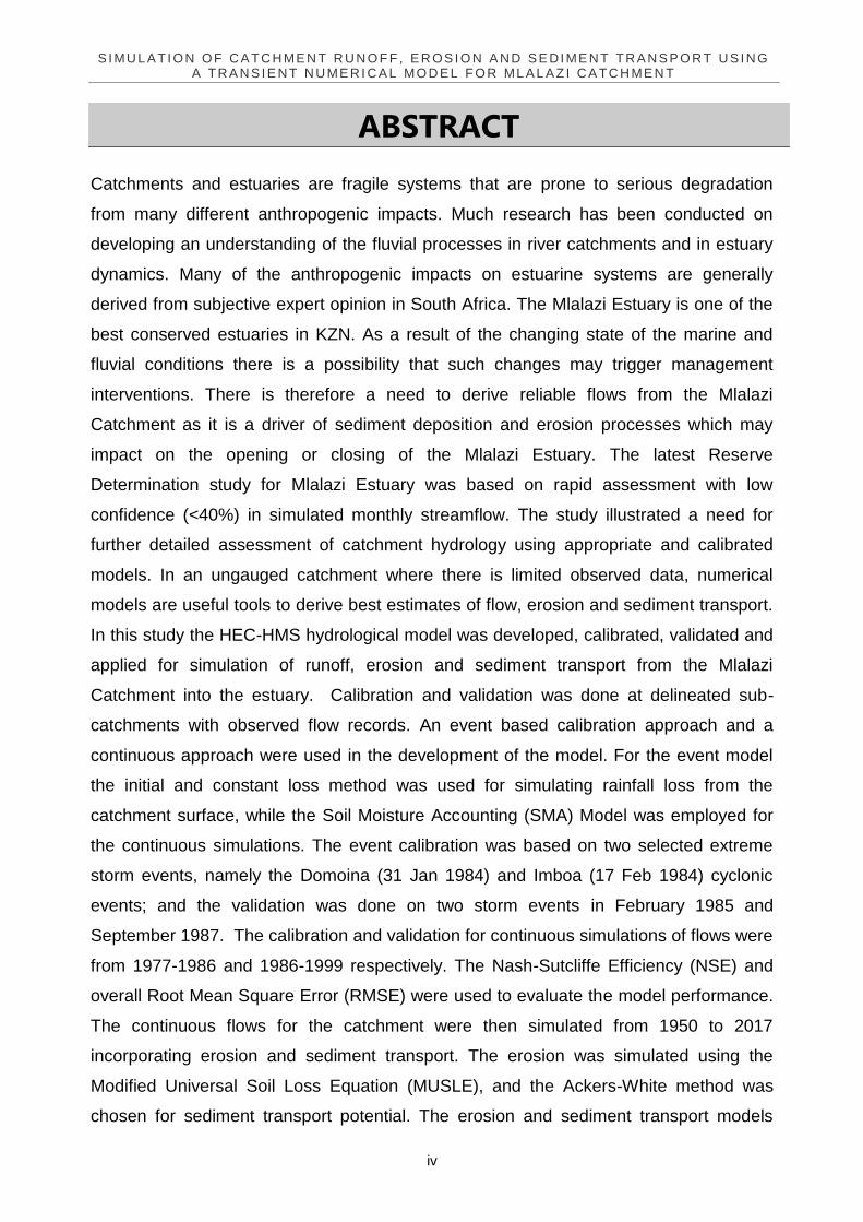
ABSTRACT
Catchments and estuaries are fragile systems that are prone to serious degradation
from many different anthropogenic impacts. Much research has been conducted on
developing an understanding of the fluvial processes in river catchments and in estuary
dynamics. Many of the anthropogenic impacts on estuarine systems are generally
derived from subjective expert opinion in South Africa. The Mlalazi Estuary is one of the
best conserved estuaries in KZN. As a result of the changing state of the marine and
fluvial conditions there is a possibility that such changes may trigger management
interventions. There is therefore a need to derive reliable flows from the Mlalazi
Catchment as it is a driver of sediment deposition and erosion processes which may
impact on the opening or closing of the Mlalazi Estuary. The latest Reserve
Determination study for Mlalazi Estuary was based on rapid assessment with low
confidence (<40%) in simulated monthly streamflow. The study illustrated a need for
further detailed assessment of catchment hydrology using appropriate and calibrated
models. In an ungauged catchment where there is limited observed data, numerical
models are useful tools to derive best estimates of flow, erosion and sediment transport.
In this study the HEC-HMS hydrological model was developed, calibrated, validated and
applied for simulation of runoff, erosion and sediment transport from the Mlalazi
Catchment into the estuary. Calibration and validation was done at delineated sub-
catchments with observed flow records. An event based calibration approach and a
continuous approach were used in the development of the model. For the event model
the initial and constant loss method was used for simulating rainfall loss from the
catchment surface, while the Soil Moisture Accounting (SMA) Model was employed for
the continuous simulations. The event calibration was based on two selected extreme
storm events, namely the Domoina (31 Jan 1984) and Imboa (17 Feb 1984) cyclonic
events; and the validation was done on two storm events in February 1985 and
September 1987. The calibration and validation for continuous simulations of flows were
from 1977-1986 and 1986-1999 respectively. The Nash-Sutcliffe Efficiency (NSE) and
overall Root Mean Square Error (RMSE) were used to evaluate the model performance.
The continuous flows for the catchment were then simulated from 1950 to 2017
incorporating erosion and sediment transport. The erosion was simulated using the
Modified Universal Soil Loss Equation (MUSLE), and the Ackers-White method was
chosen for sediment transport potential. The erosion and sediment transport models

S I MU L A TI O N O F C A TC H ME N T R U N O F F , E R OS I O N A N D S E DI ME N T TR A N S P O R T U S I N G A TR A N S I E N T N U ME R I C A L MO D E L F O R ML A L A Z I C A TC H ME N T
v
were not calibrated due to limitations of observed data, but parameter values were
estimated from other studies available in literature for this region. The simulated
sediment yield from the catchment was evaluated by comparison to sediments yield
found by other studies in this region.
It was concluded that a physically based, numerical simulation model provides a
pragmatic method for the derivation of reliable hydrodynamic data and information in
catchments with limited observed data like the Mlalazi Catchment. Furthermore, this
study allowed a smooth linkage with the study of the Mlalazi Estuary that employed the
HEC-RAS model.
S I MU L A TI O N O F C A TC H ME N T R U N O F F , E R OS I O N A N D S E DI ME N T TR A N S P O R T U S I N G A TR A N S I E N T N U ME R I C A L MO D E L F O R ML A L A Z I C A TC H ME N T
vi
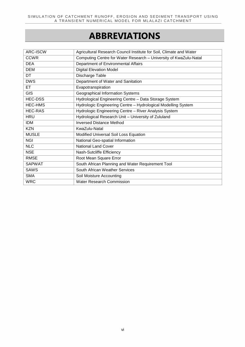
ABBREVIATIONS
ARC-ISCW Agricultural Research Council Institute for Soil, Climate and Water
CCWR Computing Centre for Water Research – University of KwaZulu-Natal
DEA Department of Environmental Affairs
DEM Digital Elevation Model
DT Discharge Table
DWS Department of Water and Sanitation
ET Evapotranspiration
GIS Geographical Information Systems
HEC-DSS Hydrological Engineering Centre – Data Storage System
HEC-HMS Hydrologic Engineering Centre – Hydrological Modelling System
HEC-RAS Hydrologic Engineering Centre – River Analysis System
HRU Hydrological Research Unit – University of Zululand
IDM Inversed Distance Method
KZN KwaZulu-Natal
MUSLE Modified Universal Soil Loss Equation
NGI National Geo-spatial Information
NLC National Land Cover
NSE Nash-Sutcliffe Efficiency
RMSE Root Mean Square Error
SAPWAT South African Planning and Water Requirement Tool
SAWS South African Weather Services
SMA Soil Moisture Accounting
WRC Water Research Commission
S I MU L A TI O N O F C A TC H ME N T R U N O F F , E R OS I O N A N D S E DI ME N T TR A N S P O R T U S I N G A TR A N S I E N T N U ME R I C A L MO D E L F O R ML A L A Z I C A TC H ME N T
vii
TABLE OF CONTENTS
DEDICATION ....................................................................................................................................................... i
DECLARATION .................................................................................................................................................. ii
ACKNOWLEDGEMENTS .................................................................................................................................. iii
ABSTRACT... ..................................................................................................................................................... iv
ABBREVIATIONS .............................................................................................................................................. vi
TABLE OF CONTENTS ................................................................................................................................... vii
LIST OF TABLES .............................................................................................................................................. ix
LIST OF FIGURES ............................................................................................................................................. x
CHAPTER 1: INTRODUCTION 1
1.1 Problem Statement 3
1.2 Aim of Study 3
1.3 Specific Objectives 4
1.4 Research Hypothesis 4
1.5 Thesis Organisation 4
CHAPTER 2: LITERATURE REVIEW 5
2.1 Hydrological Modelling 5
2.2 Different Hydrological Models 7
2.2.1 MIKE SHE Model 7
2.2.2 The ACRU Model 9
2.2.3 SHETRAN Model 11
2.2.4 SWAT Model 13
2.2.5 HEC-HMS Model 14
2.2.6 Model Selection 16
CHAPTER 3: STUDY AREA AND DATA ANALYSIS 19
3.1 Geomorphology Data 20
3.2 Climatic Data 21
3.2.1 Rainfall 22
3.2.2 Evaporation 26
3.3 River Network Data 28
3.3.1 Runoff 29
3.3.2 W1H012 Discharge Table 34
3.4 Land Use Data 37
3.5 Soils Data 40
S I MU L A TI O N O F C A TC H ME N T R U N O F F , E R OS I O N A N D S E DI ME N T TR A N S P O R T U S I N G A TR A N S I E N T N U ME R I C A L MO D E L F O R ML A L A Z I C A TC H ME N T
viii
CHAPTER 4: MODEL CONFIGURATION AND SETUP 46
4.1 Data Processing using HEC-GeoHMS 46
4.1.1 DEM and pre-processing 46
4.1.2 Sub-catchments and stream delineation 47
4.1.3 Project setup and Basin Processing 49
4.2 Model Structure and Components 49
4.3 Basin Model 51
4.3.1 Rainfall loss component 51
4.3.2 Direct runoff component 55
4.3.3 Base flow component 56
4.4 Flow Routing Model 58
4.5 Erosion and Sediment Transport Component 60
4.6 Meteorological Model 62
4.7 Flow Model Calibration and Validation 64
4.7.1 Event based approach 65
4.7.2 Continuous based approach 65
CHAPTER 5: RESULTS AND DISCUSSION 67
5.1 Flow Calibration 67
5.1.1 Event based Calibration 67
5.1.2 Continuous based Calibration 69
5.2 Flow Validation 73
5.2.1 Event based Validation 73
5.2.2 Continuous based Validation 74
5.3 Mlalazi Catchment Runoff and Sediment Simulation Results 77
CHAPTER 6: CONCLUSIONS AND RECOMMENDATIONS 88
REFERENCES 91
APPENDIX 99
S I MU L A TI O N O F C A TC H ME N T R U N O F F , E R OS I O N A N D S E DI ME N T TR A N S P O R T U S I N G A TR A N S I E N T N U ME R I C A L MO D E L F O R ML A L A Z I C A TC H ME N T
ix
LIST OF TABLES
Table 2.1: Categorisation of numerical models (from Ford and Hamilton, 1996) ........................................... 6
Table 2.2: Comparative analysis of reviewed models................................................................................... 17
Table 3.1: Rainfall station record length and altitude distribution ................................................................. 23
Table 3.2: Potential evaporation data captured ............................................................................................ 27
Table 3.3: Flow gauging stations in the study Catchment and their period of record ................................... 30
Table 3.4: Generalised Soil Pattern data Description ................................................................................... 41
Table 5.1: Calibration parameters for event calibration at W1H012 catchment ........................................... 68
Table 5.2: Auto Calibration SMA Parameters for continuous modelling ....................................................... 70
Table 5.3: Performance measures of the model ........................................................................................... 70
Table 5.4: Performance measures of the model ........................................................................................... 75
Table 5.5: Mlalazi Catchment range for MUSLE erosion model parameters, description and sources ....... 77
Table 5.6: Statistical variables of simulated flows and sediment load .......................................................... 81

S I MU L A TI O N O F C A TC H ME N T R U N O F F , E R OS I O N A N D S E DI ME N T TR A N S P O R T U S I N G A TR A N S I E N T N U ME R I C A L MO D E L F O R ML A L A Z I C A TC H ME N T
x
LIST OF FIGURES
Figure 2.1: MIKE SHE catchment hydrological processes (DHI, 2003) ........................................................... 7
Figure 2.2: ACRU model flow diagram (Schulze, 1995) ................................................................................ 10
Figure 2.3: SHETRAN model processes (SHETRAN, 2018) ......................................................................... 12
Figure 2.4: Continuous SMA algorithm (Bennett, 1998) ................................................................................ 16
Figure 3.1: Location of the study area showing the Mlalazi Catchment ......................................................... 19
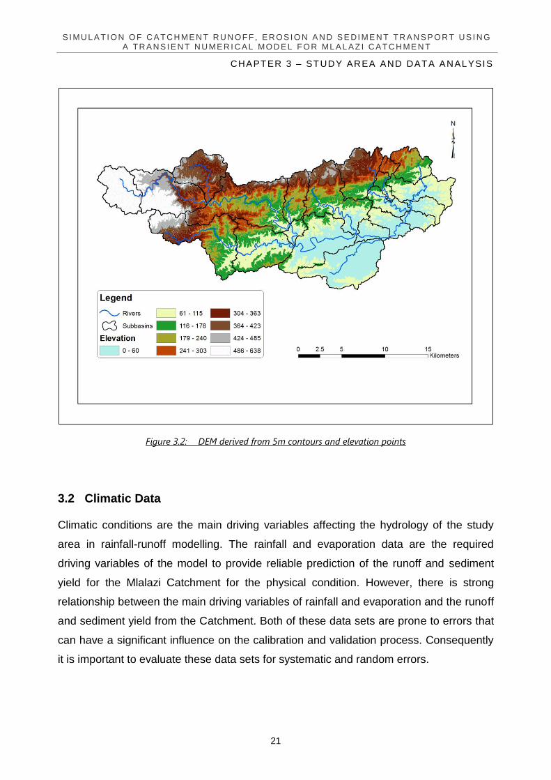
Figure 3.2: DEM derived from 5m contours and elevation points .................................................................. 21
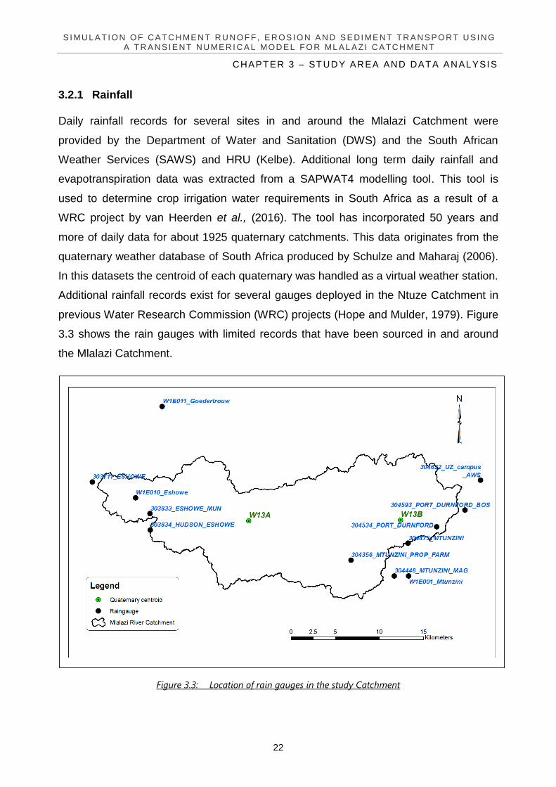
Figure 3.3: Location of rain gauges in the study Catchment .......................................................................... 22
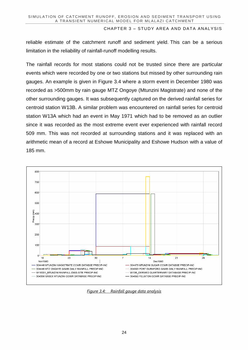
Figure 3.4: Rainfall gauge data analysis ........................................................................................................ 24
Figure 3.5: Chosen rainfall station data series ............................................................................................... 25
Figure 3.6: Catchments represented by the Quaternary Catchments ........................................................... 26
Figure 3.7: ET information derived for W13A and W13B catchments ........................................................... 27
Figure 3.8: Mlalazi River Network .................................................................................................................. 29
Figure 3.9: Main rivers and the location of the River gauging station in the study Catchment. ..................... 30
Figure 3.10: Consistency analysis for weir W1H012 (Red points –missing data) ........................................... 32
Figure 3.11: W1H012 during 1987 Flood (A) and in 2000 when it was repaired (B) (Photos by B Kelbe) ...... 34
Figure 3.12: Gauging weir W1H012 on 16 January 1981 (DWS) .................................................................... 35
Figure 3.13: Current DWS DT and fitted equation DT flows at W1H012 (Red points –missing data) ............. 37
Figure 3.14: Land use of the study Catchment (Data Source, GTI, 2015) ....................................................... 38
Figure 3.15: Commercial sugarcane land use (Source, Google Earth - 28 May 2018) ................................... 39
Figure 3.16: Subsistence farming fields (Source, Google Earth – 28 May 2018) ............................................ 39
Figure 3.17: Generalised Soil Patterns Data (Data Source, ARC-ISCW staff, 2004) ...................................... 40
Figure 3.18: Erodibility factor (Data Source, Le Roux et al., 2008) .................................................................. 42
Figure 3.19: Sub-Catchment with moderate to high erosion (A) and erosion gullies (C-D), (Google Earth –
28 May 2018) ............................................................................................................................... 43
Figure 3.20: Cover factor (Data Source, Le Roux et al., 2008) ........................................................................ 44
Figure 3.21: Topographical factor (Data Source Le Roux et al., 2008) ........................................................... 45
Figure 4.1: Sub-catchments with relatively uniform land use ......................................................................... 48
Figure 4.2: HEC-HMS Project Area for the Mlalazi Catchment generated by HEC-GeoHMS....................... 48
Figure 4.3: Main features of HEC-HMS (adapted from Cleveland, 2011)...................................................... 50
Figure 4.4: Main components of the HEC-HMS model .................................................................................. 50
Figure 4.5: Flow routing hydrographs (Cleveland, 2011) ............................................................................... 58
Figure 4.6: Illustration of the inverse-distance method .................................................................................. 63
Figure 5.1: Observed and simulated hydrographs for two storm events (Linear Scale) ................................ 68
Figure 5.2: Observed and simulated hydrographs for two storm events (Log Scale) .................................... 69
S I MU L A TI O N O F C A TC H ME N T R U N O F F , E R OS I O N A N D S E DI ME N T TR A N S P O R T U S I N G A TR A N S I E N T N U ME R I C A L MO D E L F O R ML A L A Z I C A TC H ME N T
xi
Figure 5.3: W1H015 Observed and simulated streamflow (Log Scale) ......................................................... 72
Figure 5.4: W1H015 Cumulative observed and simulated streamflow .......................................................... 72
Figure 5.5: W1H012 Observed and simulated streamflow (Log Scale) ......................................................... 72
Figure 5.6: W1H012 Cumulative observed and simulated streamflow .......................................................... 72
Figure 5.7: Observed and simulated flows for validation storm event (September 1987) ............................. 73
Figure 5.8: Observed and simulated flows for validation storm event (November 1989) .............................. 74
Figure 5.9: W1H015 validation period observed and simulated flow (Log Scale) ........................................ 76
Figure 5.10: W1H015 validation period cumulative streamflow ....................................................................... 76
Figure 5.11: W1H012 validation period observed and simulated flow (Log scale) ......................................... 76
Figure 5.12: W1H012 validation period cumulative streamflow ....................................................................... 76
Figure 5.13: Daily simulated flows (m3/s) and sediment load (tonnes/day) from Mlalazi Catchment
discharge into the Mlalazi Estuary at the confluence of the main tributaries. ............................. 79
Figure 5.14: Simulated flow depth (mm/day) and Rainfall (mm/day) ............................................................... 80
Figure 5.15: Simulated flow (m3/s) frequency plot ........................................................................................... 82
Figure 5.16: Simulated sediment yield (t/km2.a) frequency plot ....................................................................... 83
Figure 5.17: The simulated cumulative sediment load from the Mlalazi Catchment from 1950 to 2018 ......... 84
Figure 5.18: W1H004 Catchment simulated sediment grain size distribution (tonnes/day.km2) ..................... 85
Figure 5.19: W1H012 Catchment simulated sediment grain size distribution (tonnes/day.km2) ..................... 86
Figure 5.20: Mlalazi River simulated sediment grain size distribution (tonnes/day.km2) ................................. 87
S I MU L A TI O N O F C A TC H ME N T R U N O F F , E R OS I O N A N D S E DI ME N T TR A N S P O R T U S I N G A TR A N S I E N T N U ME R I C A L MO D E L F O R ML A L A Z I C A TC H ME N T
CHAPTER 1 - INTRODUCTION
1
CHAPTER 1: INTRODUCTION
Catchments and estuaries are fragile systems that are prone to serious degradation
from many different anthropogenic impacts. Much research has been conducted on
developing an understanding of the fluvial processes in river catchments and in estuary
dynamics (Chow et al., 1988). Many of the anthropogenic impacts on estuarine systems
are generally derived from subjective expert opinion in South Africa (DWS, 2015). The
ever-increasing reports of sedimentation problems in South African estuaries due to
increased sediment yields from the catchment, lead to calls for increased flushing of
these estuaries and mouth breaching, both natural and mechanical in order to remove
the sediment (CSIR, 1999 and 2003, DWS, 2015). There is a need to be more objective
in the assessment of these systems by using numerical models to provide reproducible,
comparable and consistent catchment and estuary dynamic information to evaluate
hydrological concepts and predict impacts and responses to changes in catchment
conditions (Beven, 2001). These numerical models can be a possible tool to aid in the
decision making process of dredging or artificial breaching (managing) of estuaries, in
order to prevent flooding, lower water levels, restore tidal circulation, flushing pollutants,
nutrients, and promoting migration patterns in fish and other biological resources into the
ocean, rather than to remove accumulated sediment.
Many estuaries in South Africa are only temporarily open to the sea due to the various
interactions between the fluvial and marine processes (Beck and Basson, 2008).
However, many estuaries are often closed more frequently and for longer periods than in
the past due to reduced river flows (Beck and Basson, 2008). The behaviour of these
estuary mouths is driven by three main components; river, tidal and wave processes
(O’Brian, 1931). Open-mouth conditions at small estuaries are principally maintained by
river flow and especially by a strong base flow. A reduction in minimum (base) low flow
commonly results in an increase in closed mouth conditions (Beck and Basson, 2008).
There is a need to develop relationships (models) that establish the linkages between
the estuary state and the controlling environment. In this study one of the three main
components driving the state of the estuary is in the form of river and sediment flows
through the estuary. A major contributor to the flow and sediment dynamics in the
estuary is the discharge of these hydrological components from the catchments.
S I MU L A TI O N O F C A TC H ME N T R U N O F F , E R OS I O N A N D S E DI ME N T TR A N S P O R T U S I N G A TR A N S I E N T N U ME R I C A L MO D E L F O R ML A L A Z I C A TC H ME N T
CHAPTER 1 - INTRODUCTION
2
Overland surface water flows and stream channel flows affects the landscape. Surface
flow result in erosion and sediment loads which are carried to stream channels where it
is transported to the estuary. Headwater streams with steep slopes have high velocity
which leads to stream bed erosion and rapid transport of the sediment load. Sediment
load can be carried by stream flow to the lower reaches of the catchment where they are
often deposited because of the decrease in flow velocity along a declining channel
gradient. Diversion structures and reservoirs in the catchment can also affect the
movement of sediments through the catchment where reservoirs will trap some or most
sediments which enter with the flow (USACE, 2000; Rossouw et al., 1998). The
sediment load from the catchment that is exported into the estuary can affect the estuary
bathymetry and tidal prism.
In catchments where there are no records or limited observed data of flow or sediment,
suitable rainfall-runoff and erosion models can be used as the most effective tools to
derive the best estimates of the flow and sediment loads. The resultant runoff and
sediments are routed to downstream sinks, while also modelling the erosion and the
deposition of the sediments in reservoirs and river reaches (Pak et al., 2010). Models
are useful tools for estimating flow and sedimentation in areas with limited observed
data. The Mlalazi Catchment has some flow stations on the Ntuze River tributary and
one on the upper reaches of the Mlalazi River. However, there is not a single flow station
which measures the outflows from the whole catchment. Therefore, for catchment
surface soil erosion and sediment routing studies, information from a well calibrated
rainfall-runoff model should be considered as the reliable and pragmatic approach for
estimating the discharge from the catchment into the estuary (HEC, 2015). There are no
sediment or erosion monitoring stations in the catchment.
The latest Reserve Determination study for the Mlalazi Estuary (DWS, 2015) was based
on a rapid assessment technique with low confidence for the simulated monthly flow but
produced no sediment yield for assessment. The study was based on an uncalibrated
monthly WRSM2000 (Pitman) model that was unable to provide reliable predictions of
storm and sediment yields. The study illustrated the need for further and more detailed
assessment of the catchment hydrology using appropriate and calibrated models.
S I MU L A TI O N O F C A TC H ME N T R U N O F F , E R OS I O N A N D S E DI ME N T TR A N S P O R T U S I N G A TR A N S I E N T N U ME R I C A L MO D E L F O R ML A L A Z I C A TC H ME N T
CHAPTER 1 - INTRODUCTION
3
While it is possible to measure the flow and sediment entering an estuary, these are
seldom measured in small catchments because of the cost and difficulties associated
with the measurement techniques. A more pragmatic and cost effective approach for a
clear understanding of the reality and enable future predictions is the configuration,
calibration, validation and application of a physically based continuous numerical
hydrological model (Surur, 2010). The following questions arise in the choice and
application of models:
Whether such a model can be configured and applied to the Mlalazi Catchment to
provide the transient flow and sediment yield data at the required temporal and
spatial level of accuracy for use in the Mlalazi Estuary hydrodynamic study?
What data will be required for the application of a numerical hydrological model?
Which is the most appropriate model to use with the available data?
1.1 Problem Statement
The Mlalazi Estuary is one of the best conserved estuaries in KZN (Mann, et al., 1996).
As a result of the changing state of the marine and fluvial conditions (Begg, 1978) there
is a possibility that such changes may trigger management interventions (DWS, 2015).
There is therefore a need to derive reliable flows from the Mlalazi Catchment as it is a
driver of sediment deposition and erosion processes which may impact on the opening
or closing of the Mlalazi Estuary. Catchment runoff is directly associated with climatic
and geomorphic conditions that may change in response to human induced activities
associated with land use and land cover change at the catchment scale (Day, 1981).
These changes may alter the total runoff of the catchment and therefore also impact on
the resultant opening and the closing of the estuary mouth.
1.2 Aim of Study
The aim of this study is to configure, calibrate, validate and apply a suitable numerical
hydrological model for the simulation of runoff, erosion and sediment transport from the
Mlalazi Catchment into the Mlalazi Estuary as important drivers of the hydrodynamics of
the estuary.
S I MU L A TI O N O F C A TC H ME N T R U N O F F , E R OS I O N A N D S E DI ME N T TR A N S P O R T U S I N G A TR A N S I E N T N U ME R I C A L MO D E L F O R ML A L A Z I C A TC H ME N T
CHAPTER 1 - INTRODUCTION
4
1.3 Specific Objectives
(a) Review literature on catchment hydrological models and select a suitable model
for application in the Mlalazi Catchment.
(b) Establish the required temporal resolution of the required model simulations.
(c) Identify data needs, availability and source the data required for the selected
model.
(d) Create a Digital Elevation Model (DEM), assess its accuracy for hydrological
modelling in the catchment and supplement where necessary.
(e) Calibrate and validate the model.
(f) Compute catchment flows and sediment load series to be incorporated into the
estuary model.
1.4 Research Hypothesis
Catchment runoff and sediment loads are one of the main driving variables of the
estuary mouth dynamics. An assessment of these hydrological drivers is important in
facilitating an understanding of ecological, morphological and hydrodynamic processes
in estuarine studies. A physically based, numerical simulation model is the most
pragmatic tool for the derivation of hydrodynamic information in catchments with limited
observed data.
1.5 Thesis Organisation
This thesis is organised into six chapters. The first chapter gives an introduction for the
study. The second chapter contains a literature review of hydrological models to enable
the selection of a suitable model for the study. The third chapter gives an overview of the
study area including the data available and their analysis. The fourth chapter provides
the methodologies used in the model configuration, choices of process models, the
calibration and validation of the model. The fifth chapter presents and discusses the
model results. The sixth chapter contains the conclusions reached and
recommendations.
S I MU L A TI O N O F C A TC H ME N T R U N O F F , E R OS I O N A N D S E DI ME N T TR A N S P O R T U S I N G A TR A N S I E N T N U ME R I C A L MO D E L F O R ML A L A Z I C A TC H ME N T
CHAPTER 2 – L ITERATURE REVIEW
5
CHAPTER 2: LITERATURE REVIEW
2.1 Hydrological Modelling
Models are simplified representations of specific features of the real world, predicting
effects from causes (Jewitt and Gorgens, 2000). Hydrological models are conceptual
and/or mathematical representations of the process(es) involved in the transformation of
input variables. The input variable used such as precipitation and evaporation are
transformed, through surface and subsurface transfer processes of water and energy
into hydrological outputs. The outputs include streamflow, soil moisture and groundwater
(Hughes, 2004).
In general terms, numerical models can be classified as empirical or physically-based;
deterministic or stochastics; event or continuous and furthermore, a model can be
categorised as either distributed or lumped. There is also a distinction between
measured-parameter and fitted-parameter models. This is critical for application of
hydrological models in catchments where observations of input and output are limited or
unavailable. The different categorisation of numerical models is given in Table 2.1.
The selection and configuration of the resources and process that need to be included in
the model depend on the purpose of the model application. There is not enough data to
develop an empirical model; event and continuous flow records are required; the
catchment is too large for a lumped model; so it has been established from the purpose
and review of the model and the catchment characteristics and available data that a
distributed, physical based parameterised model is the most suitable for this study.
The parameters required as input to physically-based models are generally obtained
from field measurements, maps and other sources of information (Hughes, 1991).
Physically-based numerical models are created from conceptual models which are built
upon the base knowledge of the pertinent physical, chemical and biological processes
that act on the input to produce the desired output (USACE, 2000).
S I MU L A TI O N O F C A TC H ME N T R U N O F F , E R OS I O N A N D S E DI ME N T TR A N S P O R T U S I N G A TR A N S I E N T N U ME R I C A L MO D E L F O R ML A L A Z I C A TC H ME N T
CHAPTER 2 – L ITERATURE REVIEW
6
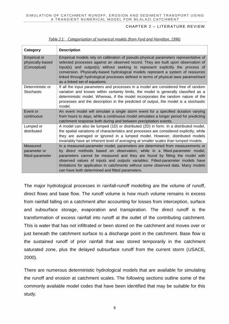
Table 2.1: Categorisation of numerical models (from Ford and Hamilton, 1996)
Category Description
Empirical or
physically-based
(Conceptual)
Empirical models rely on calibration of pseudo-physical parameters representative of
selected processes against an observed record. They are built upon observation of
input(s) and output(s) without seeking to represent explicitly the process of
conversion. Physically-based hydrological models represent a system of resources
linked through hydrological processes defined in terms of physical laws parametrised
as a linked set of equations.
Deterministic or
Stochastic
If all the input parameters and processes in a model are considered free of random
variation and known within certainty limits, the model is generally classified as a
deterministic model. Whereas, if the model incorporates the random nature of the
processes and the description in the predicted of output, the model is a stochastic
model.
Event or
continuous
An event model will simulate a single storm event for a specified duration varying
from hours to days, while a continuous model simulates a longer period for predicting
catchment response both during and between precipitation events.
Lumped or
distributed
A model can also be lumped (1D) or distributed (2D) in form. In a distributed model,
the spatial variations of characteristics and processes are considered explicitly, while
they are averaged or ignored in a lumped model. However, distributed models
invariably have an inherent level of averaging at smaller scales than lumped models.
Measured
parameter or
fitted-parameter
In a measured-parameter model, parameters are determined from measurements or
by direct methods based on observation, while in a fitted-parameter model,
parameters cannot be measured and they are found by fitting the model with
observed values of inputs and outputs variables. Fitted-parameter models have
limitations for application in catchments without some observed data. Many models
can have both determined and fitted parameters.
The major hydrological processes in rainfall-runoff modelling are the volume of runoff,
direct flows and base flow. The runoff volume is how much volume remains in excess
from rainfall falling on a catchment after accounting for losses from interception, surface
and subsurface storage, evaporation and transpiration. The direct runoff is the
transformation of excess rainfall into runoff at the outlet of the contributing catchment.
This is water that has not infiltrated or been stored on the catchment and moves over or
just beneath the catchment surface to a discharge point in the catchment. Base flow is
the sustained runoff of prior rainfall that was stored temporarily in the catchment
saturated zone, plus the delayed subsurface runoff from the current storm (USACE,
2000).
There are numerous deterministic hydrological models that are available for simulating
the runoff and erosion at catchment scales. The following sections outline some of the
commonly available model codes that have been identified that may be suitable for this
study.
S I MU L A TI O N O F C A TC H ME N T R U N O F F , E R OS I O N A N D S E DI ME N T TR A N S P O R T U S I N G A TR A N S I E N T N U ME R I C A L MO D E L F O R ML A L A Z I C A TC H ME N T
CHAPTER 2 – L ITERATURE REVIEW
7
2.2 Different Hydrological Models
2.2.1 MIKE SHE Model
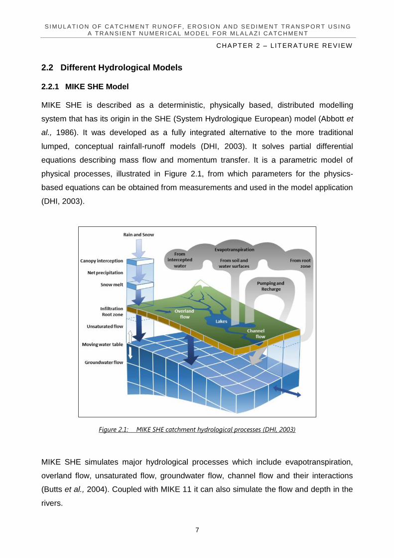
MIKE SHE is described as a deterministic, physically based, distributed modelling
system that has its origin in the SHE (System Hydrologique European) model (Abbott et
al., 1986). It was developed as a fully integrated alternative to the more traditional
lumped, conceptual rainfall-runoff models (DHI, 2003). It solves partial differential
equations describing mass flow and momentum transfer. It is a parametric model of
physical processes, illustrated in Figure 2.1, from which parameters for the physics-
based equations can be obtained from measurements and used in the model application
(DHI, 2003).
Figure 2.1: MIKE SHE catchment hydrological processes (DHI, 2003)
MIKE SHE simulates major hydrological processes which include evapotranspiration,
overland flow, unsaturated flow, groundwater flow, channel flow and their interactions
(Butts et al., 2004). Coupled with MIKE 11 it can also simulate the flow and depth in the
rivers.
S I MU L A TI O N O F C A TC H ME N T R U N O F F , E R OS I O N A N D S E DI ME N T TR A N S P O R T U S I N G A TR A N S I E N T N U ME R I C A L MO D E L F O R ML A L A Z I C A TC H ME N T
CHAPTER 2 – L ITERATURE REVIEW
8
This model is flexible in input requirement and there is no predefined list of required
input data. The required data depends on the hydrological processes which are
assumed to dominate the catchment under consideration and the process models
selected, which in turn, depend on what problems are to be solved. Basic model
parameters required for nearly every MIKE SHE model include the following:
Model extent – typically a polygon incorporating the topographical catchment
boundary
Topography – as point or gridded surface
Precipitation – as station data (rain gauge data)
Additional basic data required for runoff simulations are as follows:
Reference Evapo(transpi)ration) as station data or calculated from meteorological
data
Sub-catchment delineation – for rainfall distribution
River morphology (Geometry and cross-sections).
Land use distribution – for vegetation (Leaf Area Index (LAI), interception and
evaporation).
Soil distribution – for distributing infiltration, runoff and sediment processes.
Limitations of the MIKE SHE physical-based model:
Require significant amount of data and the cost of data acquisition may be high.
Attempts to represent flow processing at a grid scale with mathematical
description that, at best are valid for small scale experimental conditions.
Relative complexity may lead to over-parameterized descriptions for simple
applications (DHI, 2003)
The successful applications of this model are found in surface-water and groundwater
hydrology interaction applications (Refsgaard et al., 1999; Feyen et al., 2000; Andersen
et al., 2001; Vazquez and Feyen, 2003; Johnson et al., 2003).
S I MU L A TI O N O F C A TC H ME N T R U N O F F , E R OS I O N A N D S E DI ME N T TR A N S P O R T U S I N G A TR A N S I E N T N U ME R I C A L MO D E L F O R ML A L A Z I C A TC H ME N T
CHAPTER 2 – L ITERATURE REVIEW
9
The MIKE SHE model does not have any physical limit to the size of the model or model
boundary, but the mathematical descriptions applied are best suited for small scale
conditions, it is advisable to always apply the model in a distributed system. Practical
limits are that little extra detail or slightly smaller grid size will lead to long computer run
times. This is a commercial product that is not freely available, severe restrictions apply
to the model size if used without a dongle and the model runs in demo mode (DHI,
2003).
2.2.2 The ACRU Model
ACRU is a physical conceptual model. It is conceptual in that it consists of a system in
which important hydrological processes and couplings are idealized. In addition its,
physical to the degree that physical processes are represented explicitly in the process
and the model uses input variables that can be estimated from the physical
characteristics of the catchment. ACRU is therefore not a parameter fitting or optimizing
model but is critically dependent on reliable estimates of the parameter values for the
catchment to be modelled. The acronym ACRU is derived from the Agricultural
Catchments Research Unit within the Department of Agricultural Engineering of the
University of KwaZulu-Natal (UKZN), South Africa (Schulze, 1995).
Compulsory data inputs into ACRU include the catchment area, daily rainfall, reference
evaporation, soil properties and land use information that is common to most of the
similar models. Optional data can be inputted into the model based on the suitability of
the study (Schulze, 1995).
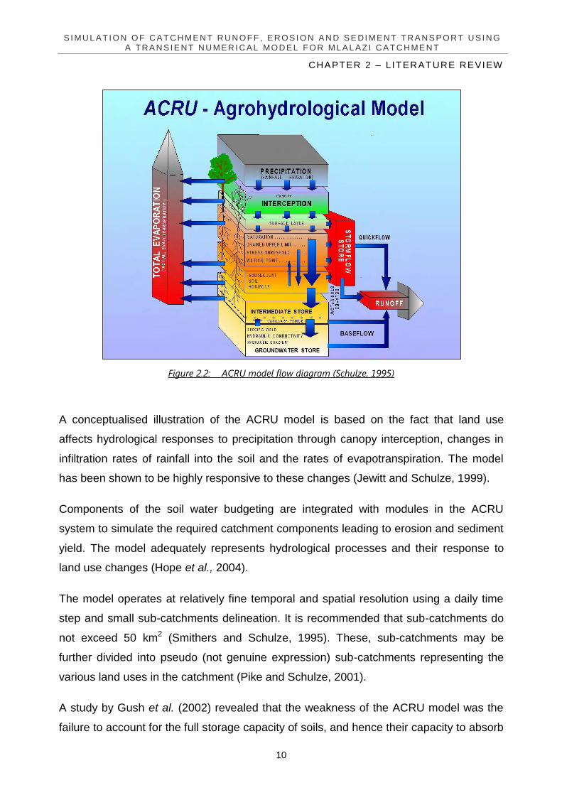
ACRU revolves around multi-layer soil water budgeting in the unsaturated zone. A flow
diagram in which multi-layer soil water budgeting is accounted for in ACRU is depicted in
Figure 2.2. In the model total streamflow (channel runoff) is generated as stormflow and
base flow depending upon the magnitude of daily rainfall in relation to dynamic soil water
budgeting. Stormflow is made up of quick overland flow and delayed stormflow. Base
flow is the sum of (unsaturated) groundwater flows and delayed through-flows, and
typically recedes much slower than the stormflow (Royappen, 2002).
S I MU L A TI O N O F C A TC H ME N T R U N O F F , E R OS I O N A N D S E DI ME N T TR A N S P O R T U S I N G A TR A N S I E N T N U ME R I C A L MO D E L F O R ML A L A Z I C A TC H ME N T
CHAPTER 2 – L ITERATURE REVIEW
10
Figure 2.2: ACRU model flow diagram (Schulze, 1995)
A conceptualised illustration of the ACRU model is based on the fact that land use
affects hydrological responses to precipitation through canopy interception, changes in
infiltration rates of rainfall into the soil and the rates of evapotranspiration. The model
has been shown to be highly responsive to these changes (Jewitt and Schulze, 1999).
Components of the soil water budgeting are integrated with modules in the ACRU
system to simulate the required catchment components leading to erosion and sediment
yield. The model adequately represents hydrological processes and their response to
land use changes (Hope et al., 2004).
The model operates at relatively fine temporal and spatial resolution using a daily time
step and small sub-catchments delineation. It is recommended that sub-catchments do
not exceed 50 km2 (Smithers and Schulze, 1995). These, sub-catchments may be
further divided into pseudo (not genuine expression) sub-catchments representing the
various land uses in the catchment (Pike and Schulze, 2001).
A study by Gush et al. (2002) revealed that the weakness of the ACRU model was the
failure to account for the full storage capacity of soils, and hence their capacity to absorb
S I MU L A TI O N O F C A TC H ME N T R U N O F F , E R OS I O N A N D S E DI ME N T TR A N S P O R T U S I N G A TR A N S I E N T N U ME R I C A L MO D E L F O R ML A L A Z I C A TC H ME N T
CHAPTER 2 – L ITERATURE REVIEW
11
rainfall following extended drying events. ACRU is based on hillslope hydrological
processes and does not incorporate groundwater dynamics. This limits its suitability for
applications in groundwater dominated systems such as Maputaland Coastal Plain in
KZN (Kelbe, pers. comm.). However, the hydrological processes in the Mlalazi
Catchment are mainly hillslope dominated and the model should be suitable for
application.
ACRU has been used widely in South Africa to assess the hydrological response of
catchments to the impacts of changing land uses and climate in the hydrological system
at varying spatial and temporal scale. Warburton, Schulze and Jewitt (2011) have done
a study which compares simulated against observed stream flow in climatically diverse
South African catchments. The study confirmed that ACRU model can be used with
confidence to simulate streamflow and represent hydrological response from a range of
climates and diversity of land uses.
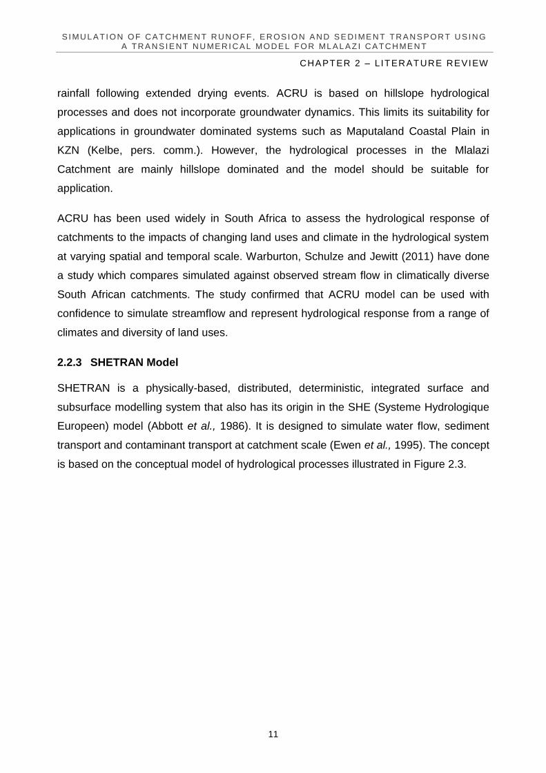
2.2.3 SHETRAN Model
SHETRAN is a physically-based, distributed, deterministic, integrated surface and
subsurface modelling system that also has its origin in the SHE (Systeme Hydrologique
Europeen) model (Abbott et al., 1986). It is designed to simulate water flow, sediment
transport and contaminant transport at catchment scale (Ewen et al., 1995). The concept
is based on the conceptual model of hydrological processes illustrated in Figure 2.3.
S I MU L A TI O N O F C A TC H ME N T R U N O F F , E R OS I O N A N D S E DI ME N T TR A N S P O R T U S I N G A TR A N S I E N T N U ME R I C A L MO D E L F O R ML A L A Z I C A TC H ME N T
CHAPTER 2 – L ITERATURE REVIEW
12
Figure 2.3: SHETRAN model processes (SHETRAN, 2018)
Essential data required for running SHETRAN are a Digital Elevation Model (DEM) with
a spatial resolution better than 50 x 50 m and a catchment mask which can be created in
GIS. Meteorological inputs include precipitation and potential evapotranspiration.
Optional data can be a vegetation map and soil category both with a maximum limit of
nine categories. River network data is automatically setup in SHETRAN from the DEM
(Ewen et al., 1995).
The time step in SHETRAN can vary throughout the simulation period, during dry
periods the time step can be relatively large (basic time step of one or two hours is often
used). During a storm event smaller time steps are used because the rates of infiltration
into the ground and surface runoff can both vary rapidly. The time step is modified based
on user-defined criteria for the rates of rainfall (Ewen et al., 1995). For each simulation,
there are three flow modules which are automatically included; namely the variable
saturation zone (VSS); evapotranspiration/interception (ET), and overland/channel (OC).
ET component calculates the net rainfall and evaporation.
VSS calculates groundwater flows in saturated zone and soil moisture in
unsaturated zone.
S I MU L A TI O N O F C A TC H ME N T R U N O F F , E R OS I O N A N D S E DI ME N T TR A N S P O R T U S I N G A TR A N S I E N T N U ME R I C A L MO D E L F O R ML A L A Z I C A TC H ME N T
CHAPTER 2 – L ITERATURE REVIEW
13
Potential evaporation is calculated using Penman’s combined energy
balance/turbulent transfer equation (Penman, 1948).
OC module calculates the depth of surface water on the ground surface and in
stream channel networks, the flow of surface water across the ground surface,
along stream channel networks and into or out of stream channels.
Both overland and channel phases of the OC module are based on the diffusive
wave approximation of the full St. Venant equations, allowing backwater effects to
be modelled.
SHETRANS, like MIKE SHE, is a commercial product with a free version that has
limitation on the size and functions available.
The SHETRAN sediment transport component simulates soil erosion by raindrop and
leaf drip impacts, detachment of soil by overland flow and channel erosion. Sediment is
transported by overland channel flows calculated in the flow component of SHETRAN,
and is routed through the sediment continuity equation (Lukey, et al., 1995).
2.2.4 SWAT Model
SWAT (Soil and Water Assessment Tool) is a river basin or catchment model developed
by Dr. Jeff Arnold for the United States Department of Agriculture (USDA) Agricultural
Research Services (ARC). This is one of the widely used catchment scale simulation
tool around the world to address catchment questions. It was developed to predict the
impacts of land management practices on water, sediment and agricultural sediment
yields in large catchments with varying soils, land use and management conditions over
long periods of time (Neitsch et al., 2011).
The SWAT model is a physical based model which requires specific information of
weather, soil properties, topography, vegetation and land management practices in a
catchment. SWAT can directly model the physical processes associated with water,
sediment and nutrient movement in catchments with limited or no monitoring data and
has been used to model the relative impact of alternative input data on water quality or
other variables. This is a semi-distributed model which allows a catchment to be divided
into a number of sub-basins that is similar to other models such as HEC-HMS. The input
information for each sub-basin is categorised into: climate; hydrological response unit,
S I MU L A TI O N O F C A TC H ME N T R U N O F F , E R OS I O N A N D S E DI ME N T TR A N S P O R T U S I N G A TR A N S I E N T N U ME R I C A L MO D E L F O R ML A L A Z I C A TC H ME N T
CHAPTER 2 – L ITERATURE REVIEW
14
ponds or wetlands; groundwater; and the main channel. Hydrological response units are
lumped catchment areas within the sub-basin that are comprised of unique land covers,
soil and management combinations (Neitsch et al., 2011).
The simulation of the hydrology of the catchment in SWAT is separated into two major
divisions: the land phase and the water or routing phase. The land phase of the
hydrologic cycle controls the amount of water, sediment, nutrient and pesticides loading
to the main channel in each sub-basin. The water or routing phase controls the
movement of water, sediments, etc. through the channel network of the catchment to the
outlet (Neitsch et al., 2011). This is an open-source model with algorithms which are
readily available and has been used in many scientific studies.
2.2.5 HEC-HMS Model
HEC-HMS is a semi-distributed conceptual hydrological model that has been developed
and used extensively by the US Army Corps of Engineers (USACE) for hydrological
studies. Like all other models, it requires precipitation, potential evapotranspiration,
runoff from the catchment (only required for calibration and validation), geographical
(geomorphic) information of the basin (for obtaining simulated runoff as output) and land
use (Sintayehu, 2015). HEC-HMS model setup consists of four main components
comprising the basin model, meteorological model, control specifications for each
simulation run, and storage of input data (time series data) (HEC, 2006).
This is a simplified distributed model, where parameters are allowed to vary in space by
dividing the basin into a number of smaller (lumped) sub-basins. The main advantage of
using HEC-HMS which is a semi-distributed model is that its structure is more
physically-based than the structure of lumped models. It is furthermore, less demanding
on input data than fully distributed models (Sintayehu, 2015).
HEC-HMS is based on a Soil Moisture Accounting (SMA) model. The SMA model is
patterned after Leavesley’s (1983) rainfall-runoff modelling system and is described in
detail in Bennett (1998). This model simulates the movement and storage of water
through the vegetation, the soil surface, the soil profile, and in (unsaturated)
groundwater layers. Given precipitation and potential evapotranspiration (ET), the model
S I MU L A TI O N O F C A TC H ME N T R U N O F F , E R OS I O N A N D S E DI ME N T TR A N S P O R T U S I N G A TR A N S I E N T N U ME R I C A L MO D E L F O R ML A L A Z I C A TC H ME N T
CHAPTER 2 – L ITERATURE REVIEW
15
computes basin surface runoff, (unsaturated) groundwater flow, losses due to ET, and
deep percolation over the entire basin (USACE, 2000).
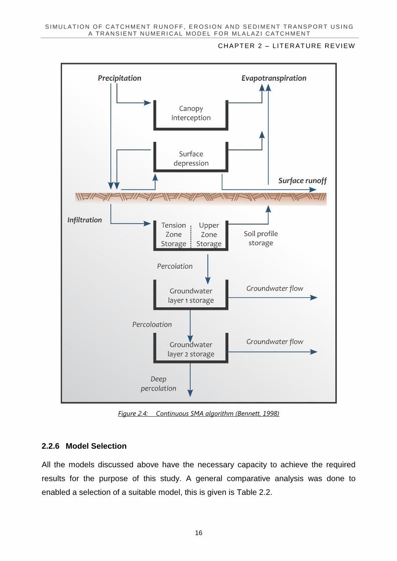
In the Soil Moisture Accounting (SMA) module showed in Figure 2.4, water is stored in
canopy leaves, in surface depressions, in soil profile, and in two groundwater layers.
Canopy interception is considered as initial loss from the incident rainfall. The infiltration
rate is subtracted from the precipitation that exceeded canopy storage (effective rainfall).
The effective rainfall that is not infiltrated is accounted for in depression storage where it
is subsequently re-distributed over time through evaporation, infiltration and runoff.
Overflow from the depression storage is considered as surface runoff (direct runoff).
Water stored in the soil profile is lost to evapotranspiration and to percolation into the
groundwater layers. The two groundwater storage layers serve as a shallow aquifer and
deep aquifer. Water in the deep aquifer moves slowly, but eventually some returns to the
channels as base flow. Lateral flow from the deep groundwater aquifer contributes to
stream base flow (Sintayehu, 2015).
HEC-HMS does not incorporate the full groundwater dynamics that are necessary in
studies in some primary aquifers (Kelbe. pers. comm.).
S I MU L A TI O N O F C A TC H ME N T R U N O F F , E R OS I O N A N D S E DI ME N T TR A N S P O R T U S I N G A TR A N S I E N T N U ME R I C A L MO D E L F O R ML A L A Z I C A TC H ME N T
CHAPTER 2 – L ITERATURE REVIEW
16
Figure 2.4: Continuous SMA algorithm (Bennett, 1998)
2.2.6 Model Selection
All the models discussed above have the necessary capacity to achieve the required
results for the purpose of this study. A general comparative analysis was done to
enabled a selection of a suitable model, this is given is Table 2.2.
S I MU L A TI O N O F C A TC H ME N T R U N O F F , E R OS I O N A N D S E DI ME N T TR A N S P O R T U S I N G A TR A N S I E N T N U ME R I C A L MO D E L F O R ML A L A Z I C A TC H ME N T
CHAPTER 2 – L ITERATURE REVIEW
17
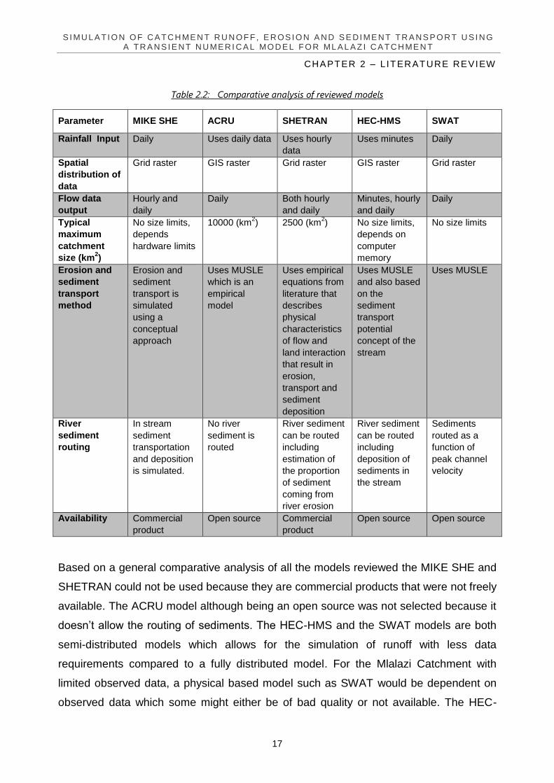
Table 2.2: Comparative analysis of reviewed models
Parameter MIKE SHE ACRU SHETRAN HEC-HMS SWAT
Rainfall Input Daily Uses daily data Uses hourly
data
Uses minutes Daily
Spatial
distribution of
data
Grid raster GIS raster Grid raster GIS raster Grid raster
Flow data
output
Hourly and
daily
Daily Both hourly
and daily
Minutes, hourly
and daily
Daily
Typical
maximum
catchment
size (km2)
No size limits,
depends
hardware limits
10000 (km2) 2500 (km
2) No size limits,
depends on
computer
memory
No size limits
Erosion and
sediment
transport
method
Erosion and
sediment
transport is
simulated
using a
conceptual
approach
Uses MUSLE
which is an
empirical
model
Uses empirical
equations from
literature that
describes
physical
characteristics
of flow and
land interaction
that result in
erosion,
transport and
sediment
deposition
Uses MUSLE
and also based
on the
sediment
transport
potential
concept of the
stream
Uses MUSLE
River
sediment
routing
In stream
sediment
transportation
and deposition
is simulated.
No river
sediment is
routed
River sediment
can be routed
including
estimation of
the proportion
of sediment
coming from
river erosion
River sediment
can be routed
including
deposition of
sediments in
the stream
Sediments
routed as a
function of
peak channel
velocity
Availability Commercial
product
Open source Commercial
product
Open source Open source
Based on a general comparative analysis of all the models reviewed the MIKE SHE and
SHETRAN could not be used because they are commercial products that were not freely
available. The ACRU model although being an open source was not selected because it
doesn’t allow the routing of sediments. The HEC-HMS and the SWAT models are both
semi-distributed models which allows for the simulation of runoff with less data
requirements compared to a fully distributed model. For the Mlalazi Catchment with
limited observed data, a physical based model such as SWAT would be dependent on
observed data which some might either be of bad quality or not available. The HEC-
S I MU L A TI O N O F C A TC H ME N T R U N O F F , E R OS I O N A N D S E DI ME N T TR A N S P O R T U S I N G A TR A N S I E N T N U ME R I C A L MO D E L F O R ML A L A Z I C A TC H ME N T
CHAPTER 2 – L ITERATURE REVIEW
18
HMS model was selected as the preferred model because it is a conceptual model
which will allow some hydrological processes to be simulated using empirical and
parameter fitting process models. This model also presented an attribute of being able
as part of river sediment routing to simulate deposition of sediments in the stream.
The model time-step ranges from minutes to daily which could allow for a storm event
simulation with ease. HEC-HMS data is spatially distributed as GIS raster which makes
it easy for data preparation and hydrological analysis in ArcMap using HEC-GeoHMS.
The model also comes with its own database storing system (DSS) which allows a
smooth link of all input datasets with the model setup.
The choice of the HEC-HMS model was also based on a careful consideration that the
selected model for rainfall-runoff, erosion and sediment transport which are drivers of
the estuary dynamics, such a model should derive information which is compatible or
allow a smooth linkage with the HEC-RAS model. The HEC-RAS model is selected in
the WRC study which this study forms part of, to route flows and sediments in the
Mlalazi Estuarty Catchment. The WRC study aims to derive estimates of flow rate, water
level and sediment transport to the Mlalazi Estuary that could influence the mouth
dynamics that lead to open or closed state. The study will allow for estuary management
interventions and application of information derived to other systems such as the Siyaya
Estuary.
S I MU L A TI O N O F C A TC H ME N T R U N O F F , E R OS I O N A N D S E DI ME N T TR A N S P O R T U S I N G A TR A N S I E N T N U ME R I C A L MO D E L F O R ML A L A Z I C A TC H ME N T
CHAPTER 3 – STUDY AREA AND DATA ANALYSIS
19
CHAPTER 3: STUDY AREA AND DATA
ANALYSIS
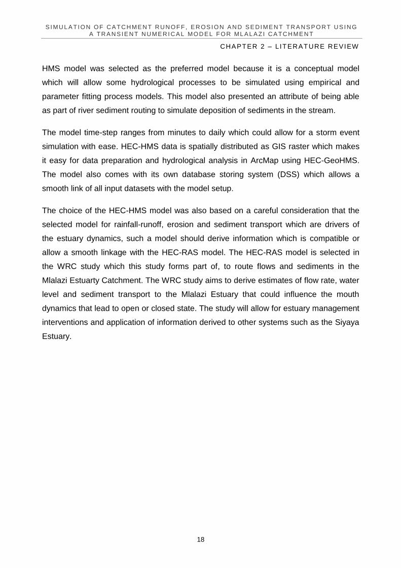
The Mlalazi Catchment is a coastal catchment that lies between the Ngoye Hills and the
Indian Ocean in the north-eastern region of South Africa. The Catchment drains into the
Mlalazi Estuary near the town of Mtunzini in northern KZN (Figure 3.1). The Mlalazi
River flows from the Ngoye Hills and comprises of two main tributaries, namely Mkukuze
River flowing in an easterly direction and KwaGugushe River (also known as Ntuze
River) which drains of the north-eastern sub-catchments. The confluence of Ntuze River
and Mlalazi River coincides with the upper reaches of the Mlalazi Estuary and forms the
outlet for this study. The Mlalazi Catchment delineated for the study covers a surface
area of 397 km2.
Figure 3.1: Location of the study area showing the Mlalazi Catchment
S I MU L A TI O N O F C A TC H ME N T R U N O F F , E R OS I O N A N D S E DI ME N T TR A N S P O R T U S I N G A TR A N S I E N T N U ME R I C A L MO D E L F O R ML A L A Z I C A TC H ME N T
CHAPTER 3 – STUDY AREA AND DATA ANALYSIS
20
3.1 Geomorphology Data
The geomorphology of a region reflects the historical processes forming the land and
water features within the catchment. Many geomorphic features can be described by the
surface elevation and drainage network. Terrain data (topography) is a critical
requirement in catchment runoff modelling. An extension tool used on an ArcGIS
platform, known as HEC-GeoHMS, uses terrain data to determine drainage paths and
some of the physical characteristics of the catchment. As part of the basin processing,
HEC-GeoHMS operates on a DEM to derive sub-basin delineation and for preparation of
hydrological input parameters. The generation of catchment drainage network in HEC-
GeoHMS can cause spurious networks due to imperfection in the DEM. It is therefore
necessary to impose the actual river network on the DEM in the processes of delineating
sub-catchment boundaries.
Five meter elevation contours and spot heights data for the study area were obtained
from the National Geo-spatial Information (NGI) section in the Department of Rural
Development and Land Reform. These datasets are much better than the SRTM
elevation datasets. The NGI data was used to create a 10 by 10 m resolution DEM
which was used for the delineation of the sub-catchments using the derived river
networks in the Mlalazi Catchment through the application of the HEC-GeoHMS
extension tool in the ArcMap platform. Figure 3.2 shows the derived DEM. The elevation
ranges from sea level at the inlet into the Mlalazi Estuary to 638 m AMSL in upper
reaches of the Ngoye Hills.
S I MU L A TI O N O F C A TC H ME N T R U N O F F , E R OS I O N A N D S E DI ME N T TR A N S P O R T U S I N G A TR A N S I E N T N U ME R I C A L MO D E L F O R ML A L A Z I C A TC H ME N T
CHAPTER 3 – STUDY AREA AND DATA ANALYSIS
21
Figure 3.2: DEM derived from 5m contours and elevation points
3.2 Climatic Data
Climatic conditions are the main driving variables affecting the hydrology of the study
area in rainfall-runoff modelling. The rainfall and evaporation data are the required
driving variables of the model to provide reliable prediction of the runoff and sediment
yield for the Mlalazi Catchment for the physical condition. However, there is strong
relationship between the main driving variables of rainfall and evaporation and the runoff
and sediment yield from the Catchment. Both of these data sets are prone to errors that
can have a significant influence on the calibration and validation process. Consequently
it is important to evaluate these data sets for systematic and random errors.
S I MU L A TI O N O F C A TC H ME N T R U N O F F , E R OS I O N A N D S E DI ME N T TR A N S P O R T U S I N G A TR A N S I E N T N U ME R I C A L MO D E L F O R ML A L A Z I C A TC H ME N T
CHAPTER 3 – STUDY AREA AND DATA ANALYSIS
22
3.2.1 Rainfall
Daily rainfall records for several sites in and around the Mlalazi Catchment were
provided by the Department of Water and Sanitation (DWS) and the South African
Weather Services (SAWS) and HRU (Kelbe). Additional long term daily rainfall and
evapotranspiration data was extracted from a SAPWAT4 modelling tool. This tool is
used to determine crop irrigation water requirements in South Africa as a result of a
WRC project by van Heerden et al., (2016). The tool has incorporated 50 years and
more of daily data for about 1925 quaternary catchments. This data originates from the
quaternary weather database of South Africa produced by Schulze and Maharaj (2006).
In this datasets the centroid of each quaternary was handled as a virtual weather station.
Additional rainfall records exist for several gauges deployed in the Ntuze Catchment in
previous Water Research Commission (WRC) projects (Hope and Mulder, 1979). Figure
3.3 shows the rain gauges with limited records that have been sourced in and around
the Mlalazi Catchment.
Figure 3.3: Location of rain gauges in the study Catchment
S I MU L A TI O N O F C A TC H ME N T R U N O F F , E R OS I O N A N D S E DI ME N T TR A N S P O R T U S I N G A TR A N S I E N T N U ME R I C A L MO D E L F O R ML A L A Z I C A TC H ME N T
CHAPTER 3 – STUDY AREA AND DATA ANALYSIS
23
The available rainfall data was captured and stored into HEC-DSSVue database tool
which is compatible to HEC-HMS. Table 3.1 shows the available rainfall stations with
records that are available for use in the meteorological model using the inverse distance
method.
Table 3.1: Rainfall station record length and altitude distribution
Name Period of observation Altitude (m)
303711 Eshowe West 06Jan1957 – 01Feb1989 595
303833 Eshowe Municipality 06Jan1957 – 01Feb1989 529
W1E010 Eshowe Dam 06Jan1957 – 28Jan1997 501
303834 Eshowe Hudson 06Jan1957 – 01Feb1989 517
W13A Quaternary covering Mkukuze tributary 01Jan1950 – 31Dec2015 332
304446 Mtunzini Magistrate 11Jan1916 – 21Oct1996 60
W1E001 Mtunzini 01Apr1969 – 30Nov1996 9
304593 Port Durnford 03Jan1949 – 16Mar2018 75
W13B Quaternary covering the Ntuze tributary 01Jan1950 – 31Dec1999 66
W1E011 Godertrouw 08May1983 - 31May2018 224
304356 Sasex Mtunzini 03Jan1966 – 29Apr1993 15
304475 Mtunzini Sugar 31Dec1946 – 29Apr1993 56
304622 UZ Campus 30Aug1975 – 30Dec1977 80
The rainfall records are derived from point source measurements (~10-3m2) of
atmospheric processes that are random in nature and variable in space and time. It is
not possible for a single point measurement to capture the spatial distribution of rainfall
at catchment scales > 50 km2. In a study of the nature of convective storm in the north
eastern region of South Africa, Kelbe (1984) established that the characteristic (average)
area of a large convective storm cell was between 50-100 km2 and lasted for an average
of 30 minutes. Although these convective cells generally combined to form a swath
across a catchment as they propagated under prevailing wind regimes, the rainfall
variability across the swath varies considerably and cannot be measured adequately by
a standard rain gauge. These typical storm areas are generally a factor of 2 smaller than
the catchment. It is necessary to have several point measurements of rainfall to
adequately represent the distribution of rainfall in a catchment in order to provide a
S I MU L A TI O N O F C A TC H ME N T R U N O F F , E R OS I O N A N D S E DI ME N T TR A N S P O R T U S I N G A TR A N S I E N T N U ME R I C A L MO D E L F O R ML A L A Z I C A TC H ME N T
CHAPTER 3 – STUDY AREA AND DATA ANALYSIS
24
reliable estimate of the catchment runoff and sediment yield. This can be a serious
limitation in the reliability of rainfall-runoff modelling results.
The rainfall records for most stations could not be trusted since there are particular
events which were recorded by one or two stations but missed by other surrounding rain
gauges. An example is given in Figure 3.4 where a storm event in December 1980 was
recorded as >500mm by rain gauge MTZ Ongoye (Mtunzini Magistrate) and none of the
other surrounding gauges. It was subsequently captured on the derived rainfall series for
centroid station W13B. A similar problem was encountered on rainfall series for centroid
station W13A which had an event in May 1971 which had to be removed as an outlier
since it was recorded as the most extreme event ever experienced with rainfall record
509 mm. This was not recorded at surrounding stations and it was replaced with an
arithmetic mean of a record at Eshowe Municipality and Eshowe Hudson with a value of
185 mm.
Figure 3.4: Rainfall gauge data analysis

S I MU L A TI O N O F C A TC H ME N T R U N O F F , E R OS I O N A N D S E DI ME N T TR A N S P O R T U S I N G A TR A N S I E N T N U ME R I C A L MO D E L F O R ML A L A Z I C A TC H ME N T
CHAPTER 3 – STUDY AREA AND DATA ANALYSIS
25
It would be necessary to use all gauge records available for this simulation study.
Unfortunately, all these gauges have variable length records with missing data and
many of them are no longer operational. The choice of methods and gauge networks for
distributing the rainfall are important criteria in the configuration of the runoff model. The
Inverse-Distance Method (IDM) used to distribute point rainfall over the Mlalazi
Catchment is the preferred method (described in detail in Chapter 4 under
Meteorological model) but it requires continuous data with no missing records that has
proved elusive to generate in this study. The stations chosen to generate rainfall series
for the simulation study was Port Durnford, centroid station W13A and W1E011 at the
Goedertrouw Dam was used to extend records from 2015 – 2018. Port Durford station
represents the more coastal region and W13A represents the inland area of the Mlalazi
Catchment. These stations were chosen after performing a consistency analysis. Since
they contain fewer gaps, they are consistent with most stations within the vicinity of the
Catchment. A plot of the rainfall series of the three chosen stations is given in Figure 3.5
to illustrate the variability between the various sites across the catchment.
Figure 3.5: Chosen rainfall station data series
S I MU L A TI O N O F C A TC H ME N T R U N O F F , E R OS I O N A N D S E DI ME N T TR A N S P O R T U S I N G A TR A N S I E N T N U ME R I C A L MO D E L F O R ML A L A Z I C A TC H ME N T
CHAPTER 3 – STUDY AREA AND DATA ANALYSIS
26
W1E011 and W13A are stations which are more inland while Port Durnford is located in
the more coastal area towards the east. It is evident from the above plot that from year
2000 to 2017 the derived station W13A and W1HE011 has recorded less rainfall
compared to the coastal station records at Port Durnford. The most extreme event
experienced in the study area was the flood in September 1987.
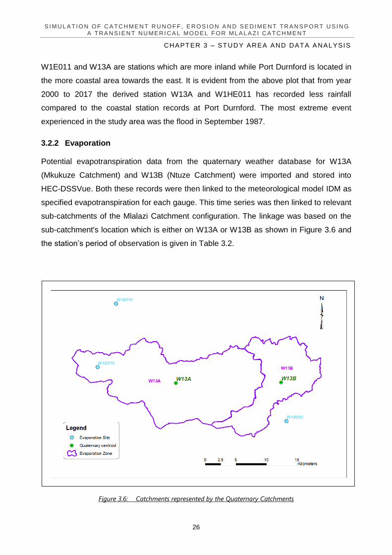
3.2.2 Evaporation
Potential evapotranspiration data from the quaternary weather database for W13A
(Mkukuze Catchment) and W13B (Ntuze Catchment) were imported and stored into
HEC-DSSVue. Both these records were then linked to the meteorological model IDM as
specified evapotranspiration for each gauge. This time series was then linked to relevant
sub-catchments of the Mlalazi Catchment configuration. The linkage was based on the
sub-catchment's location which is either on W13A or W13B as shown in Figure 3.6 and
the station’s period of observation is given in Table 3.2.
Figure 3.6: Catchments represented by the Quaternary Catchments
S I MU L A TI O N O F C A TC H ME N T R U N O F F , E R OS I O N A N D S E DI ME N T TR A N S P O R T U S I N G A TR A N S I E N T N U ME R I C A L MO D E L F O R ML A L A Z I C A TC H ME N T
CHAPTER 3 – STUDY AREA AND DATA ANALYSIS
27
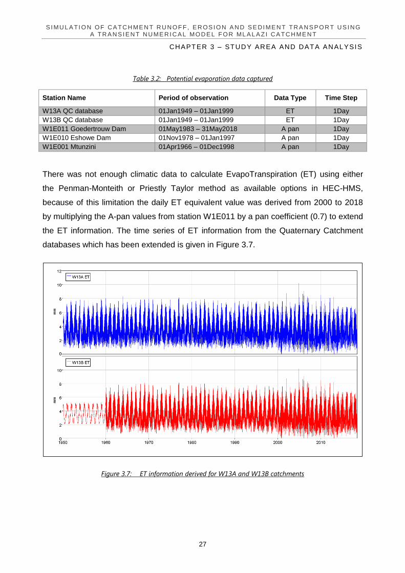
Table 3.2: Potential evaporation data captured
Station Name Period of observation Data Type Time Step
W13A QC database 01Jan1949 – 01Jan1999 ET 1Day
W13B QC database 01Jan1949 – 01Jan1999 ET 1Day
W1E011 Goedertrouw Dam 01May1983 – 31May2018 A pan 1Day
W1E010 Eshowe Dam 01Nov1978 – 01Jan1997 A pan 1Day
W1E001 Mtunzini 01Apr1966 – 01Dec1998 A pan 1Day
There was not enough climatic data to calculate EvapoTranspiration (ET) using either
the Penman-Monteith or Priestly Taylor method as available options in HEC-HMS,
because of this limitation the daily ET equivalent value was derived from 2000 to 2018
by multiplying the A-pan values from station W1E011 by a pan coefficient (0.7) to extend
the ET information. The time series of ET information from the Quaternary Catchment
databases which has been extended is given in Figure 3.7.
Figure 3.7: ET information derived for W13A and W13B catchments
S I MU L A TI O N O F C A TC H ME N T R U N O F F , E R OS I O N A N D S E DI ME N T TR A N S P O R T U S I N G A TR A N S I E N T N U ME R I C A L MO D E L F O R ML A L A Z I C A TC H ME N T
CHAPTER 3 – STUDY AREA AND DATA ANALYSIS
28
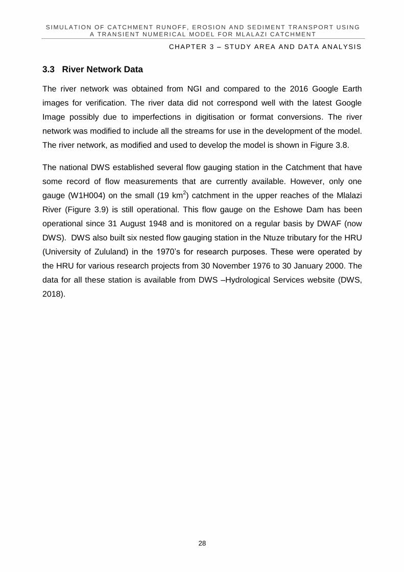
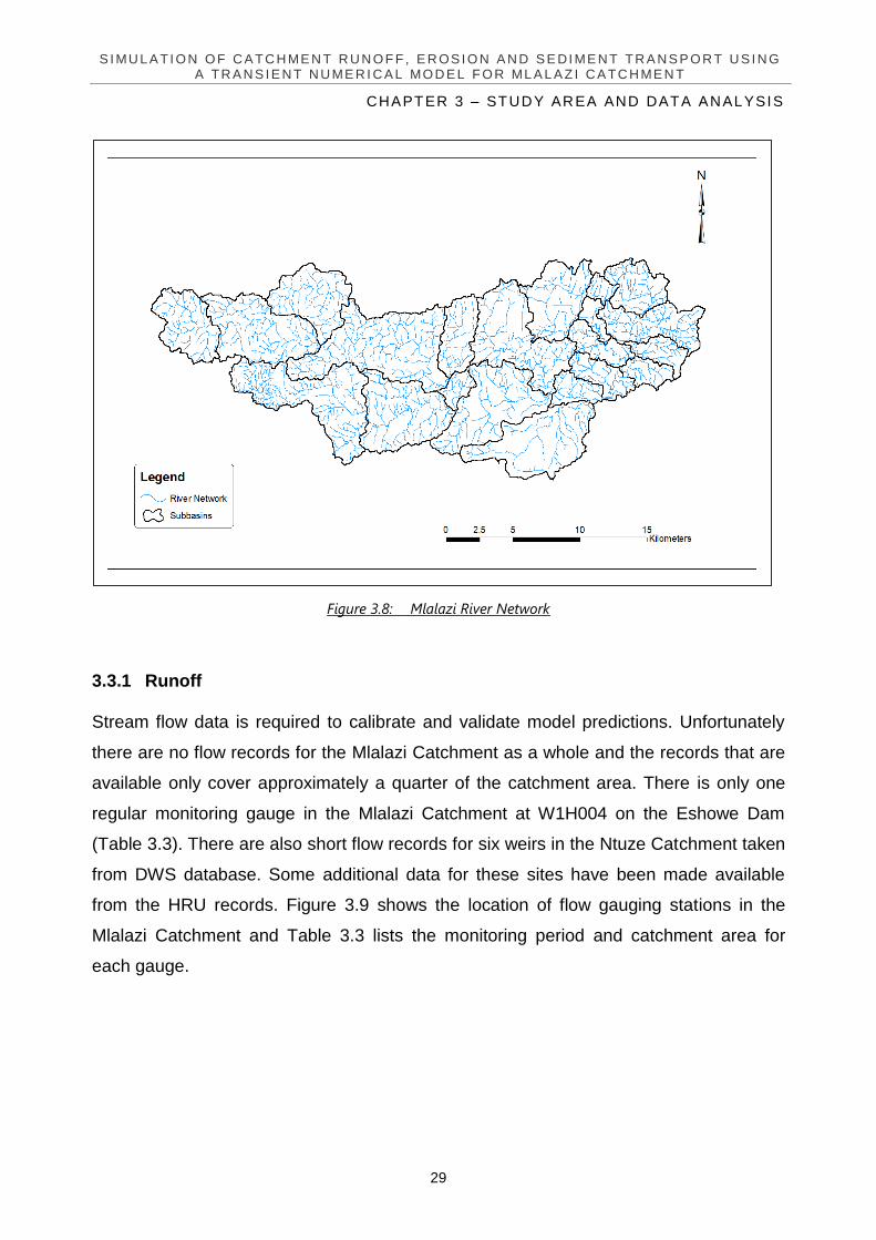
3.3 River Network Data
The river network was obtained from NGI and compared to the 2016 Google Earth
images for verification. The river data did not correspond well with the latest Google
Image possibly due to imperfections in digitisation or format conversions. The river
network was modified to include all the streams for use in the development of the model.
The river network, as modified and used to develop the model is shown in Figure 3.8.
The national DWS established several flow gauging station in the Catchment that have
some record of flow measurements that are currently available. However, only one
gauge (W1H004) on the small (19 km2) catchment in the upper reaches of the Mlalazi
River (Figure 3.9) is still operational. This flow gauge on the Eshowe Dam has been
operational since 31 August 1948 and is monitored on a regular basis by DWAF (now
DWS). DWS also built six nested flow gauging station in the Ntuze tributary for the HRU
(University of Zululand) in the 1970’s for research purposes. These were operated by
the HRU for various research projects from 30 November 1976 to 30 January 2000. The
data for all these station is available from DWS –Hydrological Services website (DWS,
2018).
S I MU L A TI O N O F C A TC H ME N T R U N O F F , E R OS I O N A N D S E DI ME N T TR A N S P O R T U S I N G A TR A N S I E N T N U ME R I C A L MO D E L F O R ML A L A Z I C A TC H ME N T
CHAPTER 3 – STUDY AREA AND DATA ANALYSIS
29
Figure 3.8: Mlalazi River Network
3.3.1 Runoff
Stream flow data is required to calibrate and validate model predictions. Unfortunately
there are no flow records for the Mlalazi Catchment as a whole and the records that are
available only cover approximately a quarter of the catchment area. There is only one
regular monitoring gauge in the Mlalazi Catchment at W1H004 on the Eshowe Dam
(Table 3.3). There are also short flow records for six weirs in the Ntuze Catchment taken
from DWS database. Some additional data for these sites have been made available
from the HRU records. Figure 3.9 shows the location of flow gauging stations in the
Mlalazi Catchment and Table 3.3 lists the monitoring period and catchment area for
each gauge.

S I MU L A TI O N O F C A TC H ME N T R U N O F F , E R OS I O N A N D S E DI ME N T TR A N S P O R T U S I N G A TR A N S I E N T N U ME R I C A L MO D E L F O R ML A L A Z I C A TC H ME N T
CHAPTER 3 – STUDY AREA AND DATA ANALYSIS
30
Figure 3.9: Main rivers and the location of the River gauging station in the study Catchment.
Table 3.3: Flow gauging stations in the study Catchment and their period of record
Station Number Period of observation Area (km2)
W1H004 Eshowe 31Aug1948 – 30Oct2015 19
W1H012 31Jul1977 - 30Jan2000 82
W1H031 30Sep1988 – 29Nov1998 3
W1H025 Eshowe 30Jun1959 – 29Nov1990
W1H013 30Nov-1976 – 30Dec1999 33
W1H014 13Nov1979 – 04Dec1988 12
W1H015 30Nov1976 – 30Dec1997 23.5
W1H017 30Nov1976 – 30Dec1997 0.65
The runoff measurements are derived from various types of hydraulic structures that
have measurement limits and require regular maintenance for a reliable data series.
These gauges represent the entire catchment and would provide a more reliable
indicator of the effective rainfall than a few point measurements. The gauge data could
S I MU L A TI O N O F C A TC H ME N T R U N O F F , E R OS I O N A N D S E DI ME N T TR A N S P O R T U S I N G A TR A N S I E N T N U ME R I C A L MO D E L F O R ML A L A Z I C A TC H ME N T
CHAPTER 3 – STUDY AREA AND DATA ANALYSIS
31
provide a method of evaluating the rainfall record(s) that have proved to be problematic
in this study as discussed earlier in this chapter. Unfortunately, the gauge data only
covers the Ntuze Catchment and a small portion of the Mlalazi Catchment at station
W1H004 on the Eshowe Dam (Eshlazi Dam). All the other gauges with exception of
W1H004 have a short monitoring period from 1977 to 1997 (Table 3.3). However, the
Ntuze gauges are nested and provide a method of verifying several storm events that do
not reflect the rainfall record at some gauges.
The gauging stations used for calibration are W1H004; W1H031; W1H015 and W1H012.
However W1H004 might not at all times show a reliable rainfall-runoff relationship since
Eshlazi Dam is located immediately upstream which was built in the early 1980s and is
used for water supply for Eshowe Town. The flow gauge which covers the largest part of
the catchment on Ntuze River is W1H012. This gauge has been used extensively in this
study for most of the calibrations and validations in order to get best estimates of runoff
and sediments yield from the Mlalazi Catchment.
Rainfall and flow data for the calibration period were plotted to analyse for consistency
and reliability of the driving variable (rainfall) and calibration data (flow). A plot of the
data is shown in Figure 3.10 for flow gauge W1H012 from August 1977 to July 1986.

S I MU L A TI O N O F C A TC H ME N T R U N O F F , E R OS I O N A N D S E DI ME N T TR A N S P O R T U S I N G A TR A N S I E N T N U ME R I C A L MO D E L F O R ML A L A Z I C A TC H ME N T
CHAPTER 3 – STUDY AREA AND DATA ANALYSIS
32
Figure 3.10: Consistency analysis for weir W1H012 (Red points –missing data)
It can be observed that the cyclonic rainfall in January and February 1984 (Domoina and
Imboa respectively) was recorded on the rainfall series and also resulted in an extreme
event at the flow station. However, in 1978 rainfall peaked to more than 100 mm but
there was no flow of such magnitude which resulted. Again in 1980 rainfall peaked to
more than 140 mm but the resultant flow did not exceed 100 m3/s. The largest
discrepancy identified was in 1985 when flows of approximately 200 m3/s were recorded
as a resultant of a small rainfall amount of only 80 mm. This analysis shows that rainfall
and resultant flows are not corresponding at all times. This could be a problem of the
reliability of rainfall data for a point source measurement, or possibly also errors in
gauge data. There are gaps of missing observed flow data from 1981 to 1983 in the
dataset.
A calculation was done on the possible catchment yield. Assuming that the catchment of
W1H012 (82 km2) had no losses (Impervious), then cyclone Domoina with rainfall of 194
mm/day when converted to mean daily flow rate will yield a flow of 183 m3/s,
substantially less than the recorded flow of 330 m3/s. Similarly, Imboa (February 1984)
S I MU L A TI O N O F C A TC H ME N T R U N O F F , E R OS I O N A N D S E DI ME N T TR A N S P O R T U S I N G A TR A N S I E N T N U ME R I C A L MO D E L F O R ML A L A Z I C A TC H ME N T
CHAPTER 3 – STUDY AREA AND DATA ANALYSIS
33
with rainfall of 178 mm/day will yield a flow of 169 m3/s. Looking at Figure 3.10 it is
evident that the two analysed events show a large discrepancy between the rainfall and
runoff measurements that needs to be analysed further.
The flow gauging station W1H012 is a compound sharp crested V-notch weir (Figure
3.11) with a specified rating table that is available on the DWS portal. The rating table
has an upper structural limit for a stage measurement of 4.78 m with a corresponding
discharge rate of 482 m3/s. Flow measurements above this stage limit cannot be
accurately determined because the weir becomes hydraulically drowned (submerged).
This is illustrated in Figure 3.11 after the peak of the Domoina Floods that reached a
maximum stage value of 8.93 m above the lower V-Notch. This could present a limitation
on all extreme events recorded which their mean stage is above the structural limit and
their flows cannot be determined using the rating table. An event recorded where the
mean daily stage exceeded the structural limit was a flood on 28 September 1987 were
the mean daily stage reached a height of 6 m. Figure 3.11 shows the station W1H012
which was submerged under water during the 1987 flood and after it was repaired in
2000.
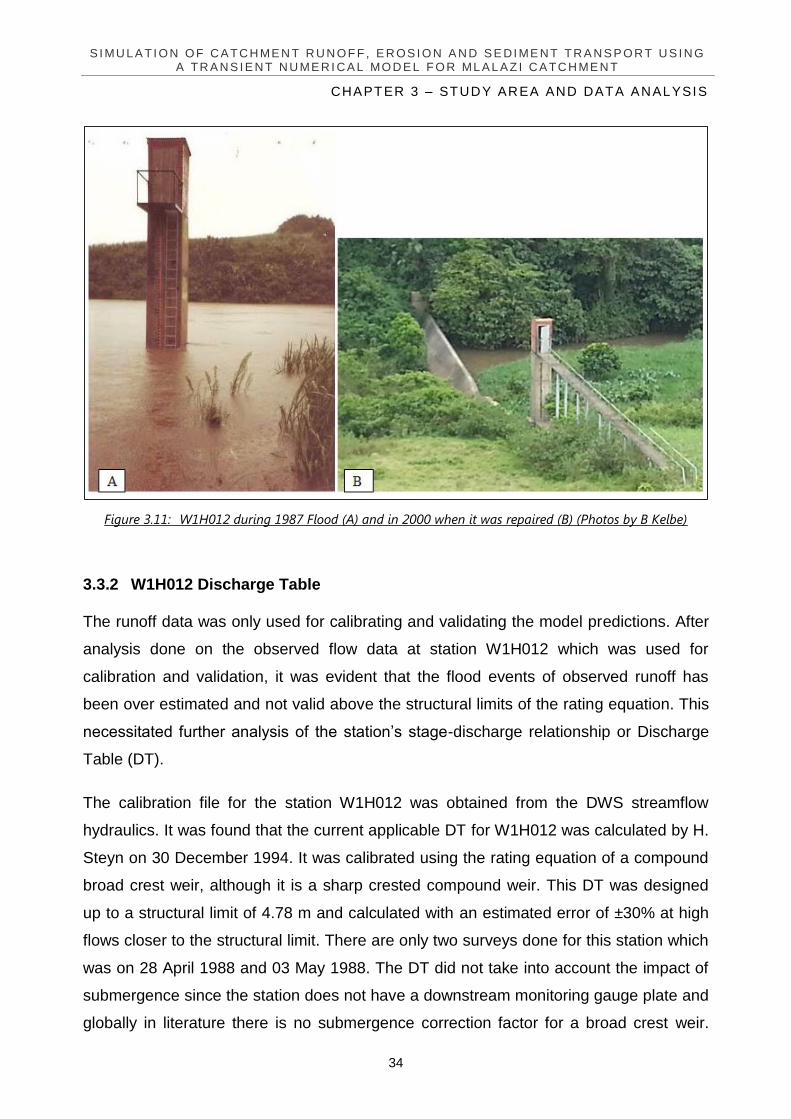
S I MU L A TI O N O F C A TC H ME N T R U N O F F , E R OS I O N A N D S E DI ME N T TR A N S P O R T U S I N G A TR A N S I E N T N U ME R I C A L MO D E L F O R ML A L A Z I C A TC H ME N T
CHAPTER 3 – STUDY AREA AND DATA ANALYSIS
34
Figure 3.11: W1H012 during 1987 Flood (A) and in 2000 when it was repaired (B) (Photos by B Kelbe)
3.3.2 W1H012 Discharge Table
The runoff data was only used for calibrating and validating the model predictions. After
analysis done on the observed flow data at station W1H012 which was used for
calibration and validation, it was evident that the flood events of observed runoff has
been over estimated and not valid above the structural limits of the rating equation. This
necessitated further analysis of the station’s stage-discharge relationship or Discharge
Table (DT).
The calibration file for the station W1H012 was obtained from the DWS streamflow
hydraulics. It was found that the current applicable DT for W1H012 was calculated by H.
Steyn on 30 December 1994. It was calibrated using the rating equation of a compound
broad crest weir, although it is a sharp crested compound weir. This DT was designed
up to a structural limit of 4.78 m and calculated with an estimated error of ±30% at high
flows closer to the structural limit. There are only two surveys done for this station which
was on 28 April 1988 and 03 May 1988. The DT did not take into account the impact of
submergence since the station does not have a downstream monitoring gauge plate and
globally in literature there is no submergence correction factor for a broad crest weir.

S I MU L A TI O N O F C A TC H ME N T R U N O F F , E R OS I O N A N D S E DI ME N T TR A N S P O R T U S I N G A TR A N S I E N T N U ME R I C A L MO D E L F O R ML A L A Z I C A TC H ME N T
CHAPTER 3 – STUDY AREA AND DATA ANALYSIS
35
Submergence of a structure starts when the downstream water level reaches the height
of the crest of the low notch and starts to have effect on the discharge assumptions of
flow through the structure. If a station is calibrated and submergence is not taken into
account, the discharge table will overestimate the flows above the level of submergence
which is unknown for this weir.
A V-notch structure is much more accurate at low flows. The error increases when one
considers the structure under submerged conditions when the assumptions of critical
flow conditions over the sharp crested notches are not valid. The compound weir
W1H012 consists of a low V-notch; other notches of sharp crest, but it is not a broad
crest as it has been calibrated by H. Steyn (Figure 3.12). The DT by H. Steyn was found
to be over-estimating high flows and therefore could not be used for calibration and
validation of the model for extreme events.
Figure 3.12: Gauging weir W1H012 on 16 January 1981 (DWS)
S I MU L A TI O N O F C A TC H ME N T R U N O F F , E R OS I O N A N D S E DI ME N T TR A N S P O R T U S I N G A TR A N S I E N T N U ME R I C A L MO D E L F O R ML A L A Z I C A TC H ME N T
CHAPTER 3 – STUDY AREA AND DATA ANALYSIS
36
In the DWS – Streamflow Hydraulics calibration file it was found that there is a DT
calculated based on a fitted equation produced from 35 current gauging’s. They were
done between 1980 and 1983 and included other points produced using a slope area
method based on surveys of flood marks. This fitted equation DT was calculated by Mr
GD Jones on 15 October 1981 up to a DT limit of 5.67m. The equation of the DT was:
𝑄 = 𝐴(𝐻 + 𝐷)𝐵 (1)
Where 𝑄 is the discharge and 𝐻 is the stage; 𝐴 = 2.27537; 𝐷 = 0.000 and 𝐵 = 2.57848.
This fitted equation had a R2 value of 0.989. This DT was considered to be more
accurate and suitable for use for this study since it was produced from more direct
methods rather than a theoretical calibration based on a set of site theoretical
requirements. A HEC-RAS calculation was thought of as a solution but it could not be
used to produce the Ha/Hb pairs to be used for submergence correction since there is a
weir structure between the point of stage measurement upstream (Ha) and a point of
stage measurement downstream (Hb).
The mean daily stage data for W1H012 was converted to discharge using Equation 1 for
the period of record and this was used for calibration and validation. Figure 3.13 shows
flows from the two DTs which also confirmed that the current DT over-estimated the
flows.
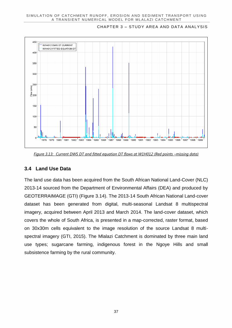
S I MU L A TI O N O F C A TC H ME N T R U N O F F , E R OS I O N A N D S E DI ME N T TR A N S P O R T U S I N G A TR A N S I E N T N U ME R I C A L MO D E L F O R ML A L A Z I C A TC H ME N T
CHAPTER 3 – STUDY AREA AND DATA ANALYSIS
37
Figure 3.13: Current DWS DT and fitted equation DT flows at W1H012 (Red points –missing data)
3.4 Land Use Data
The land use data has been acquired from the South African National Land-Cover (NLC)
2013-14 sourced from the Department of Environmental Affairs (DEA) and produced by
GEOTERRAIMAGE (GTI) (Figure 3.14). The 2013-14 South African National Land-cover
dataset has been generated from digital, multi-seasonal Landsat 8 multispectral
imagery, acquired between April 2013 and March 2014. The land-cover dataset, which
covers the whole of South Africa, is presented in a map-corrected, raster format, based
on 30x30m cells equivalent to the image resolution of the source Landsat 8 multi-
spectral imagery (GTI, 2015). The Mlalazi Catchment is dominated by three main land
use types; sugarcane farming, indigenous forest in the Ngoye Hills and small
subsistence farming by the rural community.
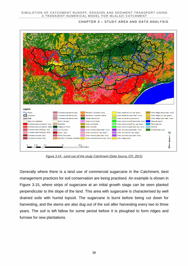
S I MU L A TI O N O F C A TC H ME N T R U N O F F , E R OS I O N A N D S E DI ME N T TR A N S P O R T U S I N G A TR A N S I E N T N U ME R I C A L MO D E L F O R ML A L A Z I C A TC H ME N T
CHAPTER 3 – STUDY AREA AND DATA ANALYSIS
38
Figure 3.14: Land use of the study Catchment (Data Source, GTI, 2015)
Generally where there is a land use of commercial sugarcane in the Catchment, best
management practices for soil conservation are being practised. An example is shown in
Figure 3.15, where strips of sugarcane at an initial growth stage can be seen planted
perpendicular to the slope of the land. This area with sugarcane is characterised by well
drained soils with humid topsoil. The sugarcane is burnt before being cut down for
harvesting, and the stems are also dug out of the soil after harvesting every two to three
years. The soil is left fallow for some period before it is ploughed to form ridges and
furrows for new plantations.
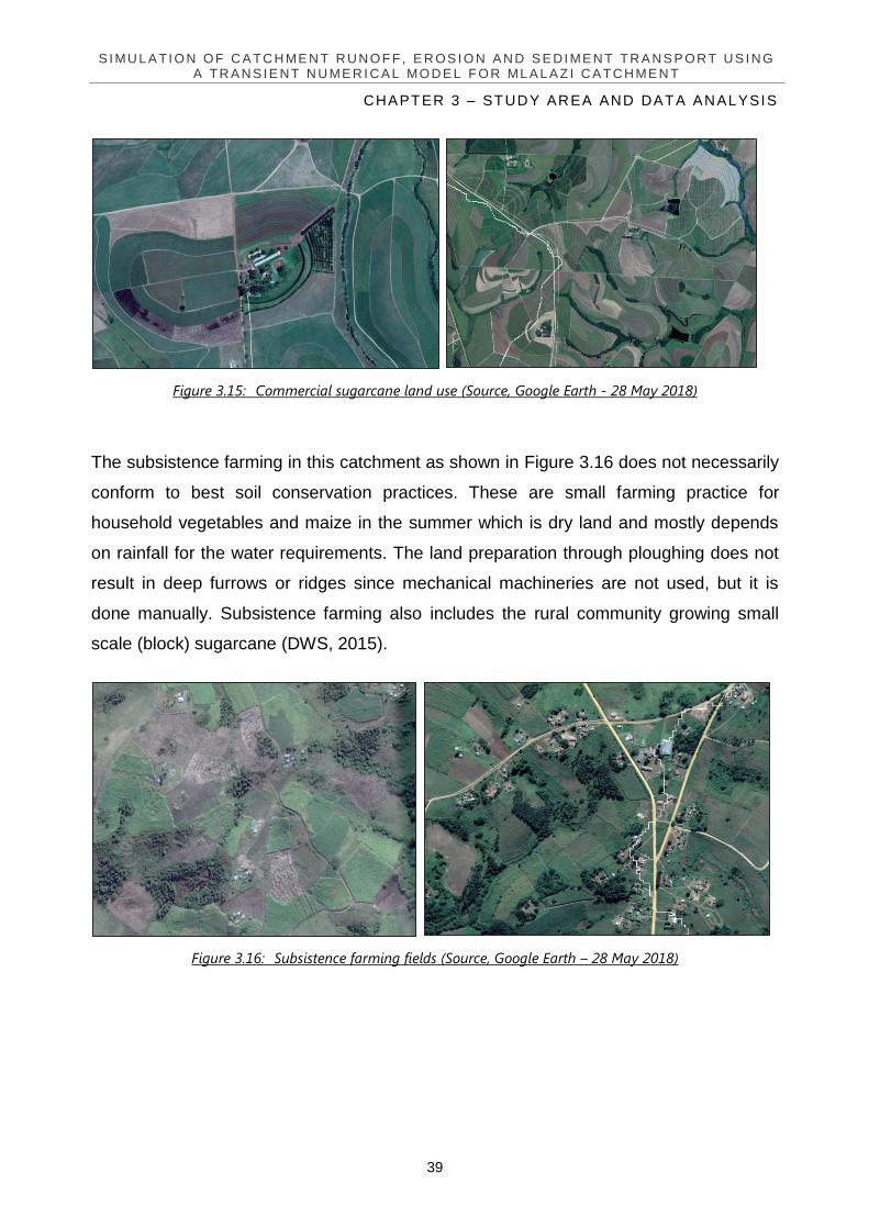
S I MU L A TI O N O F C A TC H ME N T R U N O F F , E R OS I O N A N D S E DI ME N T TR A N S P O R T U S I N G A TR A N S I E N T N U ME R I C A L MO D E L F O R ML A L A Z I C A TC H ME N T
CHAPTER 3 – STUDY AREA AND DATA ANALYSIS
39
Figure 3.15: Commercial sugarcane land use (Source, Google Earth - 28 May 2018)
The subsistence farming in this catchment as shown in Figure 3.16 does not necessarily
conform to best soil conservation practices. These are small farming practice for
household vegetables and maize in the summer which is dry land and mostly depends
on rainfall for the water requirements. The land preparation through ploughing does not
result in deep furrows or ridges since mechanical machineries are not used, but it is
done manually. Subsistence farming also includes the rural community growing small
scale (block) sugarcane (DWS, 2015).
Figure 3.16: Subsistence farming fields (Source, Google Earth – 28 May 2018)
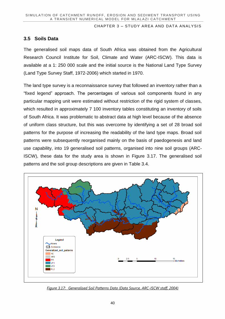
S I MU L A TI O N O F C A TC H ME N T R U N O F F , E R OS I O N A N D S E DI ME N T TR A N S P O R T U S I N G A TR A N S I E N T N U ME R I C A L MO D E L F O R ML A L A Z I C A TC H ME N T
CHAPTER 3 – STUDY AREA AND DATA ANALYSIS
40
3.5 Soils Data
The generalised soil maps data of South Africa was obtained from the Agricultural
Research Council Institute for Soil, Climate and Water (ARC-ISCW). This data is
available at a 1: 250 000 scale and the initial source is the National Land Type Survey
(Land Type Survey Staff, 1972-2006) which started in 1970.
The land type survey is a reconnaissance survey that followed an inventory rather than a
“fixed legend” approach. The percentages of various soil components found in any
particular mapping unit were estimated without restriction of the rigid system of classes,
which resulted in approximately 7 100 inventory tables constituting an inventory of soils
of South Africa. It was problematic to abstract data at high level because of the absence
of uniform class structure, but this was overcome by identifying a set of 28 broad soil
patterns for the purpose of increasing the readability of the land type maps. Broad soil
patterns were subsequently reorganised mainly on the basis of paedogenesis and land
use capability, into 19 generalised soil patterns, organised into nine soil groups (ARC-
ISCW), these data for the study area is shown in Figure 3.17. The generalised soil
patterns and the soil group descriptions are given in Table 3.4.
Figure 3.17: Generalised Soil Patterns Data (Data Source, ARC-ISCW staff, 2004)
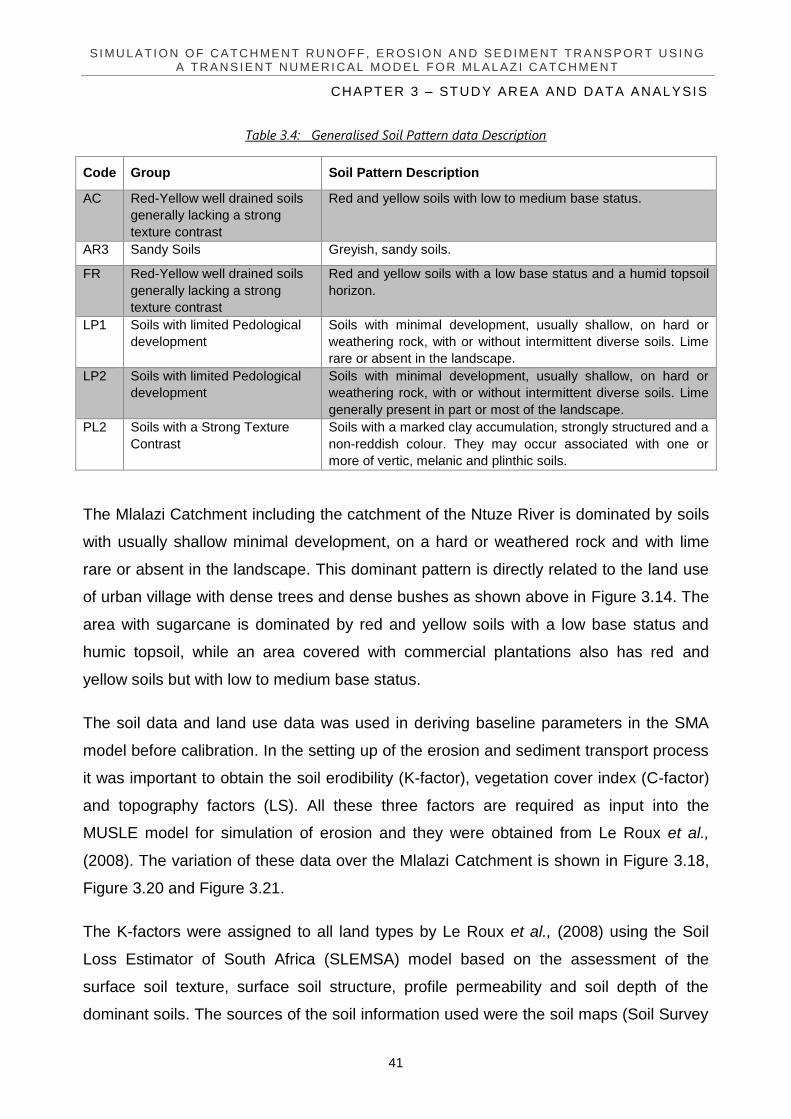
S I MU L A TI O N O F C A TC H ME N T R U N O F F , E R OS I O N A N D S E DI ME N T TR A N S P O R T U S I N G A TR A N S I E N T N U ME R I C A L MO D E L F O R ML A L A Z I C A TC H ME N T
CHAPTER 3 – STUDY AREA AND DATA ANALYSIS
41
Table 3.4: Generalised Soil Pattern data Description
Code Group Soil Pattern Description
AC Red-Yellow well drained soils
generally lacking a strong
texture contrast
Red and yellow soils with low to medium base status.
AR3 Sandy Soils Greyish, sandy soils.
FR Red-Yellow well drained soils
generally lacking a strong
texture contrast
Red and yellow soils with a low base status and a humid topsoil
horizon.
LP1 Soils with limited Pedological
development
Soils with minimal development, usually shallow, on hard or
weathering rock, with or without intermittent diverse soils. Lime
rare or absent in the landscape.
LP2 Soils with limited Pedological
development
Soils with minimal development, usually shallow, on hard or
weathering rock, with or without intermittent diverse soils. Lime
generally present in part or most of the landscape.
PL2 Soils with a Strong Texture
Contrast
Soils with a marked clay accumulation, strongly structured and a
non-reddish colour. They may occur associated with one or
more of vertic, melanic and plinthic soils.
The Mlalazi Catchment including the catchment of the Ntuze River is dominated by soils
with usually shallow minimal development, on a hard or weathered rock and with lime
rare or absent in the landscape. This dominant pattern is directly related to the land use
of urban village with dense trees and dense bushes as shown above in Figure 3.14. The
area with sugarcane is dominated by red and yellow soils with a low base status and
humic topsoil, while an area covered with commercial plantations also has red and
yellow soils but with low to medium base status.
The soil data and land use data was used in deriving baseline parameters in the SMA
model before calibration. In the setting up of the erosion and sediment transport process
it was important to obtain the soil erodibility (K-factor), vegetation cover index (C-factor)
and topography factors (LS). All these three factors are required as input into the
MUSLE model for simulation of erosion and they were obtained from Le Roux et al.,
(2008). The variation of these data over the Mlalazi Catchment is shown in Figure 3.18,
Figure 3.20 and Figure 3.21.
The K-factors were assigned to all land types by Le Roux et al., (2008) using the Soil
Loss Estimator of South Africa (SLEMSA) model based on the assessment of the
surface soil texture, surface soil structure, profile permeability and soil depth of the
dominant soils. The sources of the soil information used were the soil maps (Soil Survey
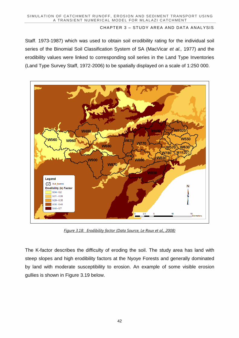
S I MU L A TI O N O F C A TC H ME N T R U N O F F , E R OS I O N A N D S E DI ME N T TR A N S P O R T U S I N G A TR A N S I E N T N U ME R I C A L MO D E L F O R ML A L A Z I C A TC H ME N T
CHAPTER 3 – STUDY AREA AND DATA ANALYSIS
42
Staff. 1973-1987) which was used to obtain soil erodibility rating for the individual soil
series of the Binomial Soil Classification System of SA (MacVicar et al., 1977) and the
erodibility values were linked to corresponding soil series in the Land Type Inventories
(Land Type Survey Staff, 1972-2006) to be spatially displayed on a scale of 1:250 000.
Figure 3.18: Erodibility factor (Data Source, Le Roux et al., 2008)
The K-factor describes the difficulty of eroding the soil. The study area has land with
steep slopes and high erodibility factors at the Nyoye Forests and generally dominated
by land with moderate susceptibility to erosion. An example of some visible erosion
gullies is shown in Figure 3.19 below.
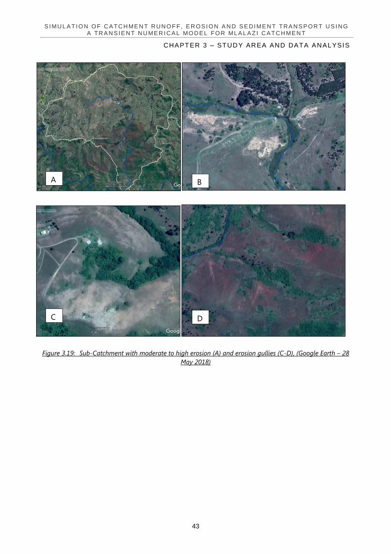
S I MU L A TI O N O F C A TC H ME N T R U N O F F , E R OS I O N A N D S E DI ME N T TR A N S P O R T U S I N G A TR A N S I E N T N U ME R I C A L MO D E L F O R ML A L A Z I C A TC H ME N T
CHAPTER 3 – STUDY AREA AND DATA ANALYSIS
43
Figure 3.19: Sub-Catchment with moderate to high erosion (A) and erosion gullies (C-D), (Google Earth – 28
May 2018)
A B
C D
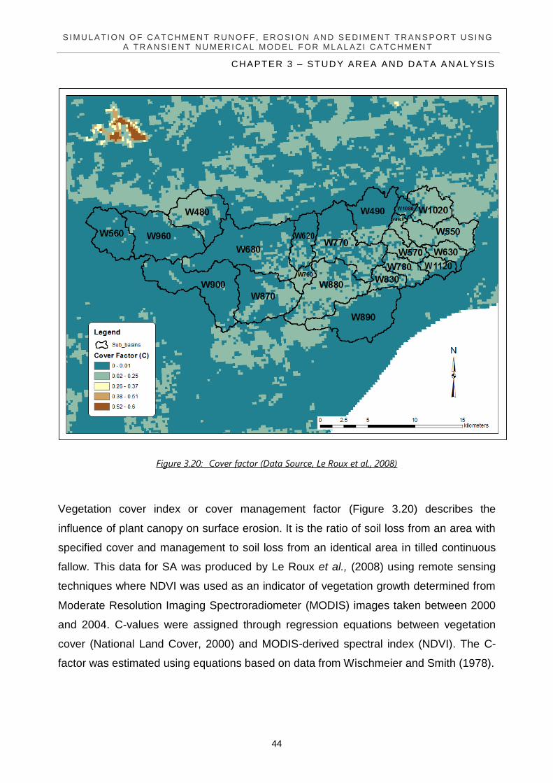
S I MU L A TI O N O F C A TC H ME N T R U N O F F , E R OS I O N A N D S E DI ME N T TR A N S P O R T U S I N G A TR A N S I E N T N U ME R I C A L MO D E L F O R ML A L A Z I C A TC H ME N T
CHAPTER 3 – STUDY AREA AND DATA ANALYSIS
44
Figure 3.20: Cover factor (Data Source, Le Roux et al., 2008)
Vegetation cover index or cover management factor (Figure 3.20) describes the
influence of plant canopy on surface erosion. It is the ratio of soil loss from an area with
specified cover and management to soil loss from an identical area in tilled continuous
fallow. This data for SA was produced by Le Roux et al., (2008) using remote sensing
techniques where NDVI was used as an indicator of vegetation growth determined from
Moderate Resolution Imaging Spectroradiometer (MODIS) images taken between 2000
and 2004. C-values were assigned through regression equations between vegetation
cover (National Land Cover, 2000) and MODIS-derived spectral index (NDVI). The C-
factor was estimated using equations based on data from Wischmeier and Smith (1978).
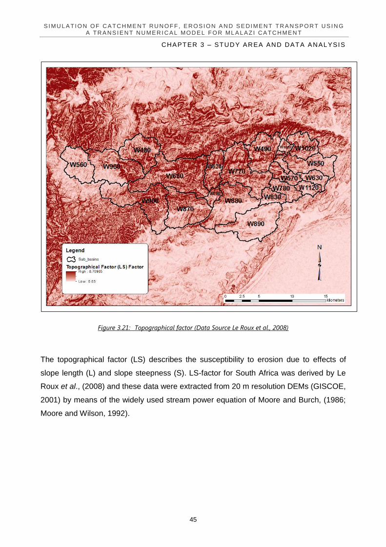
S I MU L A TI O N O F C A TC H ME N T R U N O F F , E R OS I O N A N D S E DI ME N T TR A N S P O R T U S I N G A TR A N S I E N T N U ME R I C A L MO D E L F O R ML A L A Z I C A TC H ME N T
CHAPTER 3 – STUDY AREA AND DATA ANALYSIS
45
Figure 3.21: Topographical factor (Data Source Le Roux et al., 2008)
The topographical factor (LS) describes the susceptibility to erosion due to effects of
slope length (L) and slope steepness (S). LS-factor for South Africa was derived by Le
Roux et al., (2008) and these data were extracted from 20 m resolution DEMs (GISCOE,
2001) by means of the widely used stream power equation of Moore and Burch, (1986;
Moore and Wilson, 1992).
S I MU L A TI O N O F C A TC H ME N T R U N O F F , E R OS I O N A N D S E DI ME N T TR A N S P O R T U S I N G A TR A N S I E N T N U ME R I C A L MO D E L F O R ML A L A Z I C A TC H ME N T
CHAPTER 4 – MODEL CONFIGURATION AND SETUP
46
CHAPTER 4: MODEL CONFIGURATION AND
SETUP
The configuration of the HEC-HMS model involves the setup of the physical components
of the catchment (basin) drainage network that control the flow and sediment processes.
The catchment needs to be configured as a network of discrete sub-catchments with
relatively homogeneous hydrological characteristics. The derivation, specification of
these sub-catchments and parameterised characteristics are summarised in the
following sections.
4.1 Data Processing using HEC-GeoHMS
The derivation of the sub-catchments in the study area was derived using the HEC-
GeoHMS tools in ArcGIS. HEC-GeoHMS is a set of ArcGIS tools specifically designed to
process geospatial data and create input files for HEC-HMS model. The basin model
contains discrete sub-catchments with relatively homogenous hydrological elements and
their connectivity representing the movement of water in the drainage system from
source to sink (outlet). The network configuration was derived from the topographical
features using a DEM. Spatial data preparation for the basin model was done in ArcGIS
10.2 software package, with the use of three extension tools; Spatial Analyst, 3D Analyst
and HEC-GeoHMS.
4.1.1 DEM and pre-processing
As part of developing the HEC-HMS Project components in HEC-GeoHMS, the DEM
was first reconditioned to remove imperfections using the modified river network. This
eliminates the possible undesirable side effect of fictitious islands near the stream
centreline. The DEM reconditioning method allows the user to adjust the elevation of the
stream cell based on the input of a river network. A hydrologically corrected and
depressionless DEM was created by filling the artificial depressions or pits by increasing
the elevation of the pit cells to the level of the surrounding terrain; this is done to remove
imperfections of the DEM created using various interpolation routines that can create
minor artificial features in the surface.
S I MU L A TI O N O F C A TC H ME N T R U N O F F , E R OS I O N A N D S E DI ME N T TR A N S P O R T U S I N G A TR A N S I E N T N U ME R I C A L MO D E L F O R ML A L A Z I C A TC H ME N T
CHAPTER 4 – MODEL CONFIGURATION AND SETUP
47
4.1.2 Sub-catchments and stream delineation
The hydrologically corrected DEM is used as the starting point for delineating sub-
catchments and river reaches. It was used as an input to derive eight spatial layers
(datasets) that collectively describe the drainage pattern of the watershed and allows for
stream and sub-catchment delineation. The first five datasets derived were grid layers
that represent the flow direction in each cell, flow accumulation over connected cells,
stream network, stream segmentation, and watershed delineation.
Flow direction defines the direction of the steepest descent for each terrain cell
(raster pixel).
Flow accumulation determines the number of upstream cells draining to a given
cell that defines the drainage area upstream of the cell.
The main channel characteristics within each sub-catchment and the stream
channels (segments) linking each sub-catchment with specified accumulation
levels, are derived from the network of sub-catchments.
Stream segmentation divides the stream grid into segments or linkage channels
which are the sections of the stream that connect two successive junctions
(confluence), a junction and an outlet, or a junction and the drainage divide.
Drainage areas with a flow accumulation greater than a user-defined threshold are used
to establish the network of sub-catchments. The sub-catchments represent areas that
should have relatively uniform hydrological characteristics such as land use and can be
represented by one parameter value (Figure 4.1). The default of one per cent of the
largest drainage area in the entire DEM was used to establish the initial network of sub-
catchment that generally has uniform characteristics. The smaller the size threshold
specified the greater the number of sub-catchments to be delineated. However, several
of the Ntuze sub-catchments were configured to coincide with the weir catchments with
the exception of the three smallest gauges (W1H014, W1H016 and W1H017). A
schematic of the stream network is shown in Figure 4.2.
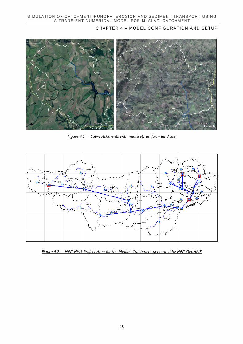
S I MU L A TI O N O F C A TC H ME N T R U N O F F , E R OS I O N A N D S E DI ME N T TR A N S P O R T U S I N G A TR A N S I E N T N U ME R I C A L MO D E L F O R ML A L A Z I C A TC H ME N T
CHAPTER 4 – MODEL CONFIGURATION AND SETUP
48
Figure 4.1: Sub-catchments with relatively uniform land use
Figure 4.2: HEC-HMS Project Area for the Mlalazi Catchment generated by HEC-GeoHMS
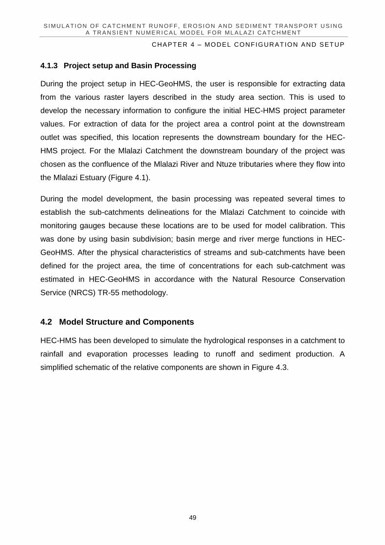
S I MU L A TI O N O F C A TC H ME N T R U N O F F , E R OS I O N A N D S E DI ME N T TR A N S P O R T U S I N G A TR A N S I E N T N U ME R I C A L MO D E L F O R ML A L A Z I C A TC H ME N T
CHAPTER 4 – MODEL CONFIGURATION AND SETUP
49
4.1.3 Project setup and Basin Processing
During the project setup in HEC-GeoHMS, the user is responsible for extracting data
from the various raster layers described in the study area section. This is used to
develop the necessary information to configure the initial HEC-HMS project parameter
values. For extraction of data for the project area a control point at the downstream
outlet was specified, this location represents the downstream boundary for the HEC-
HMS project. For the Mlalazi Catchment the downstream boundary of the project was
chosen as the confluence of the Mlalazi River and Ntuze tributaries where they flow into
the Mlalazi Estuary (Figure 4.1).
During the model development, the basin processing was repeated several times to
establish the sub-catchments delineations for the Mlalazi Catchment to coincide with
monitoring gauges because these locations are to be used for model calibration. This
was done by using basin subdivision; basin merge and river merge functions in HEC-
GeoHMS. After the physical characteristics of streams and sub-catchments have been
defined for the project area, the time of concentrations for each sub-catchment was
estimated in HEC-GeoHMS in accordance with the Natural Resource Conservation
Service (NRCS) TR-55 methodology.
4.2 Model Structure and Components
HEC-HMS has been developed to simulate the hydrological responses in a catchment to
rainfall and evaporation processes leading to runoff and sediment production. A
simplified schematic of the relative components are shown in Figure 4.3.
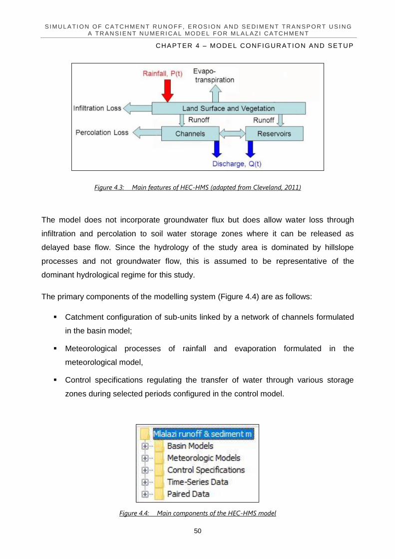
S I MU L A TI O N O F C A TC H ME N T R U N O F F , E R OS I O N A N D S E DI ME N T TR A N S P O R T U S I N G A TR A N S I E N T N U ME R I C A L MO D E L F O R ML A L A Z I C A TC H ME N T
CHAPTER 4 – MODEL CONFIGURATION AND SETUP
50
Figure 4.3: Main features of HEC-HMS (adapted from Cleveland, 2011)
The model does not incorporate groundwater flux but does allow water loss through
infiltration and percolation to soil water storage zones where it can be released as
delayed base flow. Since the hydrology of the study area is dominated by hillslope
processes and not groundwater flow, this is assumed to be representative of the
dominant hydrological regime for this study.
The primary components of the modelling system (Figure 4.4) are as follows:
Catchment configuration of sub-units linked by a network of channels formulated
in the basin model;
Meteorological processes of rainfall and evaporation formulated in the
meteorological model,
Control specifications regulating the transfer of water through various storage
zones during selected periods configured in the control model.
Figure 4.4: Main components of the HEC-HMS model
S I MU L A TI O N O F C A TC H ME N T R U N O F F , E R OS I O N A N D S E DI ME N T TR A N S P O R T U S I N G A TR A N S I E N T N U ME R I C A L MO D E L F O R ML A L A Z I C A TC H ME N T
CHAPTER 4 – MODEL CONFIGURATION AND SETUP
51
The meteorological model calculates the precipitation and evaporation series for each
sub-catchment of the basin model. HEC-HMS requires the specification of simulation
controls for each run.
Control specifications are one of the main components in the configuration of the HEC-
HMS project. Their principle purpose is to control when simulations start and stop, and
what time interval is used in the simulations. In addition to these three components of
the HEC-HMS model system is the times series data and the paired data component.
The time-series and paired data component establishes the data base for input data
required as parameters or boundary conditions in the basin and meteorological models
4.3 Basin Model
The basin model simulates the flow of precipitation through the canopy with interception
losses from evaporation, surface storage/ponding on the hillslope, infiltration and
percolation storage. Deep percolated water can returned to stream channel as base
flow, the runoff to sub-catchment outlet and erosion on hillslope. The Basin model was
setup for both event and continuous simulations with the difference being in the rainfall
loss and the base flow component selected.
4.3.1 Rainfall loss component
For the event simulation, the initial and constant-rate loss method was selected for
calculating losses. According to USACE (2000) this method has been used successfully
in hundreds of studies throughout the USA. It is easy to setup and use and includes
only a few parameters necessary to explain the variation in runoff volumes. This method
does predict total losses well and can be applied only on catchments with observed data
since it lacks direct physical relationship of parameters and catchment properties.
The SMA method was not selected for event modelling because a detailed account of
the movement and storage of water through the system was not necessary for single
storms. According to USACE (2000) the SCS CN method does not consider rainfall
intensity and the infiltration rate continuously decreases towards zero during storms of
long duration. The deficit and constant method is recommended for long term
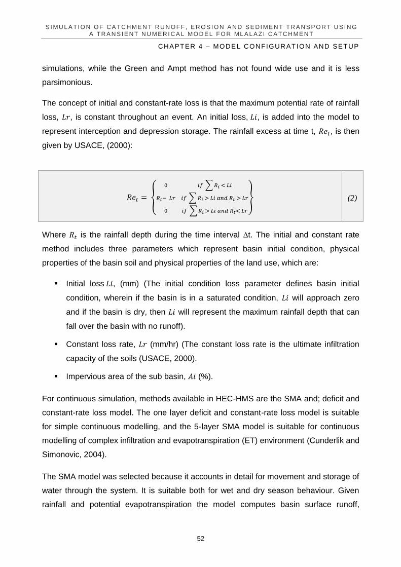
S I MU L A TI O N O F C A TC H ME N T R U N O F F , E R OS I O N A N D S E DI ME N T TR A N S P O R T U S I N G A TR A N S I E N T N U ME R I C A L MO D E L F O R ML A L A Z I C A TC H ME N T
CHAPTER 4 – MODEL CONFIGURATION AND SETUP
52
simulations, while the Green and Ampt method has not found wide use and it is less
parsimonious.
The concept of initial and constant-rate loss is that the maximum potential rate of rainfall
loss, 𝐿𝑟, is constant throughout an event. An initial loss, 𝐿𝑖, is added into the model to
represent interception and depression storage. The rainfall excess at time t, 𝑅𝑒𝑡, is then
given by USACE, (2000):
𝑅𝑒𝑡 = {
0 𝑖𝑓 ∑ 𝑅𝑖 < 𝐿𝑖
𝑅𝑡− 𝐿𝑟 𝑖𝑓 ∑ 𝑅𝑖 > 𝐿𝑖 𝑎𝑛𝑑 𝑅𝑡 > 𝐿𝑟
0 𝑖𝑓 ∑ 𝑅𝑖 > 𝐿𝑖 𝑎𝑛𝑑 𝑅𝑡< 𝐿𝑟
} (2)
Where 𝑅𝑡 is the rainfall depth during the time interval ∆t. The initial and constant rate
method includes three parameters which represent basin initial condition, physical
properties of the basin soil and physical properties of the land use, which are:
Initial loss 𝐿𝑖, (mm) (The initial condition loss parameter defines basin initial
condition, wherein if the basin is in a saturated condition, 𝐿𝑖 will approach zero
and if the basin is dry, then 𝐿𝑖 will represent the maximum rainfall depth that can
fall over the basin with no runoff).
Constant loss rate, 𝐿𝑟 (mm/hr) (The constant loss rate is the ultimate infiltration
capacity of the soils (USACE, 2000).
Impervious area of the sub basin, 𝐴𝑖 (%).
For continuous simulation, methods available in HEC-HMS are the SMA and; deficit and
constant-rate loss model. The one layer deficit and constant-rate loss model is suitable
for simple continuous modelling, and the 5-layer SMA model is suitable for continuous
modelling of complex infiltration and evapotranspiration (ET) environment (Cunderlik and
Simonovic, 2004).
The SMA model was selected because it accounts in detail for movement and storage of
water through the system. It is suitable both for wet and dry season behaviour. Given
rainfall and potential evapotranspiration the model computes basin surface runoff,

S I MU L A TI O N O F C A TC H ME N T R U N O F F , E R OS I O N A N D S E DI ME N T TR A N S P O R T U S I N G A TR A N S I E N T N U ME R I C A L MO D E L F O R ML A L A Z I C A TC H ME N T
CHAPTER 4 – MODEL CONFIGURATION AND SETUP
53
groundwater flow, losses due to ET, and deep percolation over the entire basin (USACE,
2000).
The SMA model is based on Leavesley et al. (1983) Precipitation-Runoff Modelling
System. In the SMA model, the river catchment is represented by a series of
interconnected storage layers. There are four different storages in the SMA Model:
Canopy-interception storage (rainfall captured on trees, shrubs and grasses that
is lost to evaporation and does not reach the soil profile).
Surface-depression storage (water held in shallow surface depressions that is
subsequently lost to evaporation or delayed infiltration).
Soil-profile storage, 𝑆𝑠 (water stored in the top soil layer; water held in soil pores
and water attached to soil particles due to tension).
Groundwater storage, 𝐺𝑠 (model can include either one or two groundwater
storage layers that act as storage of shallow surface drainage water and deep
percolation water).
The SMA model computes flow into, out off, and in between the storages as follows
(USACE, 2000):
a) Precipitation: This is a direct input to the SMA system.
b) Evapotranspiration (ET). ET is modelled as vaporization of water directly from the
soil and vegetative surface, and transpiration through plant leaves. In the SMA
model, potential ET demand is computed from monthly pan evaporation depths,
multiplied by monthly-varying pan correction coefficients, and scaled to the time
interval. When ET is from interception storage, surface-depression storage or from
upper soil zone, actual ET (𝐴𝐸𝑇) is equivalent to potential ET (𝑃𝐸𝑇). When 𝑃𝐸𝑇 is
drawn from the tension zone, the 𝐴𝐸𝑇 is a percentage of the PET (USACE, 2000):
𝐴𝐸𝑇 = 𝑃𝐸𝑇 . 𝑓(𝐶𝑇𝑠, 𝑇𝑠) (3)
S I MU L A TI O N O F C A TC H ME N T R U N O F F , E R OS I O N A N D S E DI ME N T TR A N S P O R T U S I N G A TR A N S I E N T N U ME R I C A L MO D E L F O R ML A L A Z I C A TC H ME N T
CHAPTER 4 – MODEL CONFIGURATION AND SETUP
54
Where CTs is the current tension zone storage and 𝑇𝑠 is the maximum tension zone
storage. ET is modelled in HEC-HMS only if no precipitation occurs, if precipitation
occurs during the time interval, ET is not modelled.
c) Infiltration: The SMA model computes the potential infiltration volume (𝑃𝐼𝑉), as:
𝑃𝐼𝑉 = 𝐼𝑓 − 𝐶𝑆𝑠
𝑆𝑠𝐼𝑓
(4)
Where 𝐼𝑓 is the maximum soil infiltration rate, 𝐶𝑆𝑠 is the current soil storage, and 𝑆𝑠 is
the maximum soil storage.
d) Percolation. The percolation rate from soil profile into groundwater layer 1, CSp, is
computed as:
𝐶𝑆𝑝 = 𝑆𝑝 (𝐶𝑆𝑠
𝑆𝑠) (1 −
𝐶𝐺𝑠
𝐺𝑠)
(5)
Where 𝑆𝑝 is the maximum soil percolation rate, 𝐶𝑆𝑠 is the current soil storage, 𝑆𝑠 is the
maximum soil storage, CGs is the current storage in the groundwater layer 1, and 𝐺𝑠 is
the maximum storage in groundwater layer 1. Similarly, the percolation rate from
groundwater layer 1 to 2, 𝐶𝐺𝑝 is given by:
𝐶𝐺𝑝 = 𝐺𝑝 (𝐶𝐺𝑠
𝐺𝑠) (1 −
𝐶𝐺𝑠
𝐺𝑠)
(6)
Where 𝐺𝑝 is the maximum groundwater percolation rate.
e) Surface Runoff: Surface runoff is the Precipitation-Interception rate that exceeds the
infiltration rate and overflows the surface depression storage. This volume of water is
direct runoff.
f) Groundwater flow. The rate of groundwater flow is computed as:
𝐺𝑊𝑡+1 = 𝐶𝑆𝑝 + 𝐺𝑠𝑡 − 𝑃𝐺𝑝𝑖 − 0.5𝐺𝑤𝑡 . 𝑇
𝑅𝐺𝑠𝑖 + 0.5𝑇𝑆
(7)

S I MU L A TI O N O F C A TC H ME N T R U N O F F , E R OS I O N A N D S E DI ME N T TR A N S P O R T U S I N G A TR A N S I E N T N U ME R I C A L MO D E L F O R ML A L A Z I C A TC H ME N T
CHAPTER 4 – MODEL CONFIGURATION AND SETUP
55
Where 𝐺𝑊𝑡 , is the groundwater flow rate at the beginning of the time interval t, 𝐶𝑆𝑝 is
the actual soil percolation rate, 𝑃𝐺𝑝𝑖 is the potential percolation rate from groundwater
layer i, 𝑅𝐺𝑠𝑖 is the groundwater flow routing coefficient from storage i, and T is the
simulation time step. The volume of groundwater from the river basin is computed as:
𝐺𝑊 = 0.5(𝐺𝑊𝑡+1 + 𝐺𝑊𝑡)T (8)
4.3.2 Direct runoff component
The direct runoff component refers to the transformation of excess rainfall into point
runoff (direct runoff) from the sub-catchment channel outlet. USACE (2000) provides
general recommendations for choosing a direct runoff method with options depending
upon availability of information for calibration or parameter estimation, appropriateness
of model assumptions and user preference and experience. The Clark unit hydrograph
(Clark, 1945) was selected to calculate the direct runoff for event and continuous
simulation. This is a frequently used technique for modelling direct runoff resulting from
individual storm events (Sabol, 1988, Nelson et al., 1999, Fleming and Neary, 2004).
The method is particularly valuable for unusually shaped catchments containing several
different physiographic areas (Sabol, 1988). It has also been used by Mulder and Kelbe
(1991).
The kinetic-wave method and Mod Clark method are other options in HEC-HMS, the
kinetic-wave method is based a conceptual model which is data intensive and based on
a finite difference equations, while the Mod Clark is a distributed parameter model which
can be used with gridded data.
The same Clark unit hydrograph method used for event simulations was also used for
the continuous model to transform excess rainfall into direct runoff. The water that
exceeds the infiltration rate and overflows the surface depression storage in the SMA
model is the input to direct runoff component. The parameters for this method are the
time of concentration and the surface storage coefficient that can be estimated
through calibration if observed rainfall and streamflow data is available.
S I MU L A TI O N O F C A TC H ME N T R U N O F F , E R OS I O N A N D S E DI ME N T TR A N S P O R T U S I N G A TR A N S I E N T N U ME R I C A L MO D E L F O R ML A L A Z I C A TC H ME N T
CHAPTER 4 – MODEL CONFIGURATION AND SETUP
56
The Clark unit hydrograph method derives a catchment unit hydrograph by representing
two key processes in transformation of excess rainfall to runoff: translation and
attenuation:
Translation is based on a synthetic time-area histogram and the time of
concentration, 𝑇𝑐. The time-area histogram specifies the basin area contributing
to flow at the outlet as a function of time.
Attenuation is modelled with a linear reservoir method (HEC, 2006). The reservoir
represents the aggregated impacts of all basin storage, 𝑆𝑡. The average outflow
from the reservoir during a period t is given by (USACE, 2000) :
𝑂𝑡 = 𝐶𝐴𝐼𝑡 + 𝐶𝐵𝑂𝑡−1 (9)
Where 𝐼𝑡 is the inflow to storage at time, t and 𝐶𝐴 and 𝐶𝐵 are routing coefficients given
by:
𝐶𝐴 = ∆𝑡
𝑆𝑡 + 0.5∆𝑡 𝑎𝑛𝑑 𝐶𝐵 = 1 − 𝐶𝐴 (10)
Where ∆𝑡 is the computational time step. The required parameters of the Clark method
are:
Time of concentration, 𝑇𝑐 (hr)
Storage coefficient, 𝑆𝑡 (hr)
4.3.3 Base flow component
Base flow is the sustained runoff of prior rainfall that was stored temporarily in the
catchment soil (subsurface) profile, from the current storm (USACE, 2000). Base flow
can also have a component of flow of water that returns to the stream or land surface
from groundwater aquifers. The HEC-HMS model includes three methods for modelling
base flow: constant monthly, exponential recession and linear reservoir volume
accounting model (Cunderlik and Simonovic, 2004).
In events modelling, base flow plays a significant role in the formation of flood
hydrograph. Base flow component is important for modelling recession limbs of flood
S I MU L A TI O N O F C A TC H ME N T R U N O F F , E R OS I O N A N D S E DI ME N T TR A N S P O R T U S I N G A TR A N S I E N T N U ME R I C A L MO D E L F O R ML A L A Z I C A TC H ME N T
CHAPTER 4 – MODEL CONFIGURATION AND SETUP
57
hydrographs as well as for more accurate estimation of flood volumes (Cunderlik and
Simonovic, 2004). The exponential recession method was selected for modelling base
flow in event simulations. This is because the method is also often used as a technique
for base flow separation and groundwater recharge estimation (Arnold et al., 2000). This
method is suitable for basins where the volume and timing of base flow is strongly
influenced by rainfall events (USACE, 2000).
Other methods included in HEC-HMS for base flow modelling is the constant monthly
and linear reservoir. The latter method can only be used in conjunction with the SMA
loss method. The constant monthly method is a simple approach that uses a constant
base flow at all simulation time step falling within a particular month.
The recession model has been used often to explain the drainage from a natural storage
in a catchment (Linsley, et al., 1982). It defines the relationship of 𝐵𝑡, the base flow at
any time t, to an initial value as:
𝐵𝑡 = 𝐵𝑖 . 𝑅𝑐𝑡 (11)
Where 𝐵𝑖 is the initial base flow at time 𝑡𝑜, and 𝑅𝑐 is the exponential decay constant.
The parameters of the recession method are:
Initial base flow, 𝐵𝑖
Recession constant, 𝑅𝑐
Threshold, 𝑇𝑑
The initial flow is equal to the base flow at the beginning of the simulation. The recession
constant describes the rate of base flow decay. It is the ratio of base flow at time t to the
base flow one day earlier (t-1). The threshold is the point on the hydrograph where base
flow replaces overland flow as a source of flow from the basin (USACE, 2000).
The linear-reservoir base flow model was selected for use in conjunction with the
continuous SMA model for continuous simulations. In this model, outflows from the SMA
groundwater layers are inflows to base flow linear reservoirs. The outflow from the two
linear reservoirs is combined to compute the total base flow for the catchment. The
required parameters of the linear reservoir base flow model are:
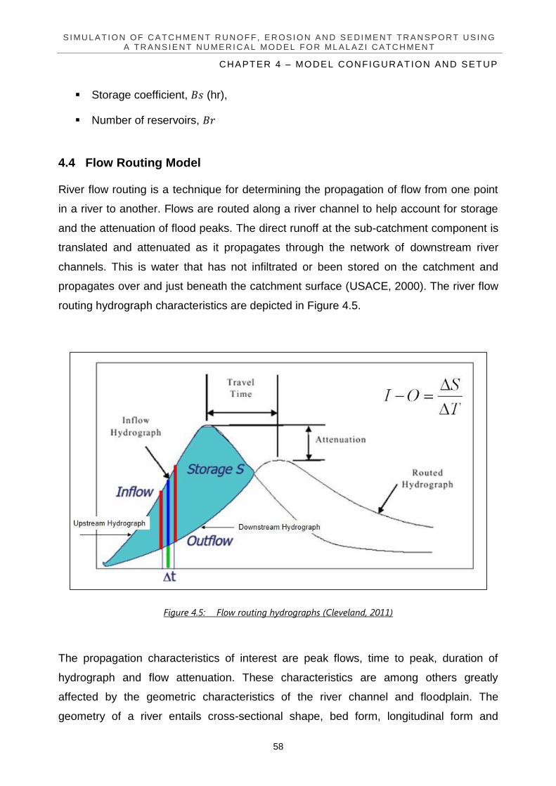
S I MU L A TI O N O F C A TC H ME N T R U N O F F , E R OS I O N A N D S E DI ME N T TR A N S P O R T U S I N G A TR A N S I E N T N U ME R I C A L MO D E L F O R ML A L A Z I C A TC H ME N T
CHAPTER 4 – MODEL CONFIGURATION AND SETUP
58
Storage coefficient, 𝐵𝑠 (hr),
Number of reservoirs, 𝐵𝑟
4.4 Flow Routing Model
River flow routing is a technique for determining the propagation of flow from one point
in a river to another. Flows are routed along a river channel to help account for storage
and the attenuation of flood peaks. The direct runoff at the sub-catchment component is
translated and attenuated as it propagates through the network of downstream river
channels. This is water that has not infiltrated or been stored on the catchment and
propagates over and just beneath the catchment surface (USACE, 2000). The river flow
routing hydrograph characteristics are depicted in Figure 4.5.
Figure 4.5: Flow routing hydrographs (Cleveland, 2011)
The propagation characteristics of interest are peak flows, time to peak, duration of
hydrograph and flow attenuation. These characteristics are among others greatly
affected by the geometric characteristics of the river channel and floodplain. The
geometry of a river entails cross-sectional shape, bed form, longitudinal form and
S I MU L A TI O N O F C A TC H ME N T R U N O F F , E R OS I O N A N D S E DI ME N T TR A N S P O R T U S I N G A TR A N S I E N T N U ME R I C A L MO D E L F O R ML A L A Z I C A TC H ME N T
CHAPTER 4 – MODEL CONFIGURATION AND SETUP
59
branching. In mathematical representations the river is represented by a simple cross-
sectional shape, such as rectangular, triangular or trapezoidal, and this cross-section is
assumed to be prismatic over the river under consideration (Singh, 2004). Flow routing
in rivers is governed by the laws of conservation of mass, momentum and energy which
is expressed as continuity, momentum and energy equations.
Flow routing models can be broadly classified into hydrologic and hydraulic models.
Hydrologic models are based on a spatially lumped form of the continuity equation and
express storage as a function of inflow and outflow (Singh, 1988). This equation does
not explicitly involve any spatial variability and expresses the flow routing variable as a
function of only time at a particular location. Lumped flow routing models includes the
Modified Puls, Muskingum method and a series of reservoir models. Hydraulic models
are based on the full or simplified version of the St. Venant equations. The simplified
hydraulic models include the kinetic wave, diffusive wave, gravity wave, and quasi-
steady state (Singh, 2004). Flows in hydraulic models are calculated as a function of
space and time throughout the system.
There are six methods included in the HEC-HMS model to compute river routing: (1) lag,
(2) kinematic wave, (3) modified Puls, (4) Muskingum, (5) Muskingum-Cunge standard
section, and (6) Muskingum-Cunge 8-point section. The Muskingum-Cunge which is a
hydrologic flow routing model was selected for river flow routing. This model is popular
and easy to use, but the main advantage of choosing a hydrologic approach is that it
greatly improves computational efficiency and speed, and reduces the amount of detail
field data that traditionally would be required for hydraulic flow routing models
(Weinmann and Laurenson, 1979). The Muskingum-Cunge model also has an
advantage over other hydrologic techniques such as Modified Puls or the simple
Muskingum method as it is comparable to the diffusion wave routing (Cunge, 1969;
Miller and Cunge, 1975); it produces consistent result which are reproducible and its
coefficients are physically based (Cunge, 1969). This model does not simulate
backwater events (Reid, 2009), however the study area does not have significant
tributary inflows or dams that could cause backwater effects.
S I MU L A TI O N O F C A TC H ME N T R U N O F F , E R OS I O N A N D S E DI ME N T TR A N S P O R T U S I N G A TR A N S I E N T N U ME R I C A L MO D E L F O R ML A L A Z I C A TC H ME N T
CHAPTER 4 – MODEL CONFIGURATION AND SETUP
60
The Muskingum-Cunge model is based upon solution of the continuity equation and the
diffusion form of the momentum equation. The combination of the two equations using a
linear approximation yields the convective diffusion equation (Miller and Cunge, 1975).
4.5 Erosion and Sediment Transport Component
Soil erosion and sedimentation deposition by water involves the processes of soil
detachment, transport, and deposition of sediment over a surface. Detachment of
sediment from the soil surface is as a result of raindrop impact and overland flow.
Rainfall detachment is caused by the locally intense shear stresses generated at the soil
surface by raindrop impact (Loch and Silburn, 1996), while overland flow causes a shear
stress to the soil surface which if it exceeds the cohesive strength of the soil (critical
shear stress) also results in sediment detachment.
There are four main types of erosion processes: sheet, rill, gully and instream erosion.
For simplification in erosion modelling, sheet erosion and rill erosion are often
considered together as overland flow erosion detaching sediment from the soil surface
only (Merritt, et al., 2003). Raindrop impact is not an important factor in terms of flow
resistance or sediment particle detachment for gully flows (Bennett, 1974). Instream
erosion involves the direct removal of sediment from stream banks (lateral erosion) or
the stream bed due to the erosive capacity of the flowing water. All these erosion types
do not necessarily occur in isolation from one another. They are influenced by the
landscape factors as well as rainfall characteristics. The dominant erosion processes
would be expected to follow a downslope sequence of splash-sheet-rill-gully (Loch and
Silburn, 1996). In many catchments worldwide, gully erosion has been identified as
being a major source of sediments entering the waterways as they usually have high
delivery ratios when well connected to streams (Merritt, et al., 2003).
A prime reason for selecting the HEC-HMS model is its ability to simulate erosion and
sediment transport component. In HEC-HMS each erosion method computes the total
sediment load out of a sub-basin during a storm and deposited into the channel at the
catchment outlet. The available methods in HEC-HMS for simulating soil erosion from
the catchment are the Modified Universal Soil Loss Equation (MUSLE) and the Build-up
wash-off erosion method. The latter is designated for urban environments and was not
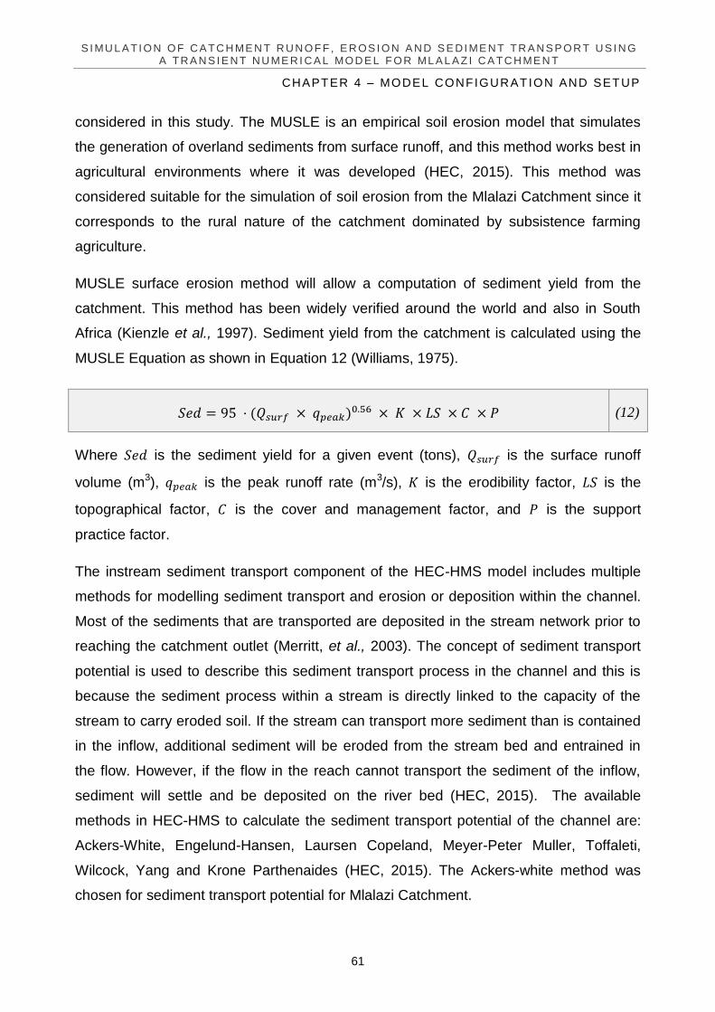
S I MU L A TI O N O F C A TC H ME N T R U N O F F , E R OS I O N A N D S E DI ME N T TR A N S P O R T U S I N G A TR A N S I E N T N U ME R I C A L MO D E L F O R ML A L A Z I C A TC H ME N T
CHAPTER 4 – MODEL CONFIGURATION AND SETUP
61
considered in this study. The MUSLE is an empirical soil erosion model that simulates
the generation of overland sediments from surface runoff, and this method works best in
agricultural environments where it was developed (HEC, 2015). This method was
considered suitable for the simulation of soil erosion from the Mlalazi Catchment since it
corresponds to the rural nature of the catchment dominated by subsistence farming
agriculture.
MUSLE surface erosion method will allow a computation of sediment yield from the
catchment. This method has been widely verified around the world and also in South
Africa (Kienzle et al., 1997). Sediment yield from the catchment is calculated using the
MUSLE Equation as shown in Equation 12 (Williams, 1975).
𝑆𝑒𝑑 = 95 ⋅ (𝑄𝑠𝑢𝑟𝑓 × 𝑞𝑝𝑒𝑎𝑘)0.56 × 𝐾 × 𝐿𝑆 × 𝐶 × 𝑃 (12)
Where 𝑆𝑒𝑑 is the sediment yield for a given event (tons), 𝑄𝑠𝑢𝑟𝑓 is the surface runoff
volume (m3), 𝑞𝑝𝑒𝑎𝑘 is the peak runoff rate (m3/s), 𝐾 is the erodibility factor, 𝐿𝑆 is the
topographical factor, 𝐶 is the cover and management factor, and 𝑃 is the support
practice factor.
The instream sediment transport component of the HEC-HMS model includes multiple
methods for modelling sediment transport and erosion or deposition within the channel.
Most of the sediments that are transported are deposited in the stream network prior to
reaching the catchment outlet (Merritt, et al., 2003). The concept of sediment transport
potential is used to describe this sediment transport process in the channel and this is
because the sediment process within a stream is directly linked to the capacity of the
stream to carry eroded soil. If the stream can transport more sediment than is contained
in the inflow, additional sediment will be eroded from the stream bed and entrained in
the flow. However, if the flow in the reach cannot transport the sediment of the inflow,
sediment will settle and be deposited on the river bed (HEC, 2015). The available
methods in HEC-HMS to calculate the sediment transport potential of the channel are:
Ackers-White, Engelund-Hansen, Laursen Copeland, Meyer-Peter Muller, Toffaleti,
Wilcock, Yang and Krone Parthenaides (HEC, 2015). The Ackers-white method was
chosen for sediment transport potential for Mlalazi Catchment.
S I MU L A TI O N O F C A TC H ME N T R U N O F F , E R OS I O N A N D S E DI ME N T TR A N S P O R T U S I N G A TR A N S I E N T N U ME R I C A L MO D E L F O R ML A L A Z I C A TC H ME N T
CHAPTER 4 – MODEL CONFIGURATION AND SETUP
62
Sediment transport includes the deposition and additional stream bed erosion, these
processes are simulated by the sediment routing method. The channel sediment routing
methods available in HEC-HMS includes, Fishers Dispersion, Linear Reservoir, Uniform
equilibrium and Volume Ratio (HEC, 2015). For the Mlalazi Catchment the volume ratio
method was used, it links the transport of sediment to the transport of flow in the channel
using a conceptual approach. This method models relatively large distances between
calculation point well (HEC, 2015). For each time interval, sediment from the upstream
elements is added to the sediment already in the reach. The deposition or erosion of the
sediment is calculated for each grain size to determine the available sediment for
routing. The proportion of available sediment that leaves the reach is assumed equal to
the proportion of stream flow that leaves the reach during the same interval. It means
that all grain sizes are transported through the reach at the same rate, even though
erosion and deposition are determined separately for each grain size.
The level of complexity introduced through the selection of the various sub-model
options is dependent on the available data or information for the study area. Many of the
parameter values required for these various options are unknown and/or obtained from
other studies presented in the hydrological literature. Consequently, it is necessary to
calibrate or validate the parameter during the development of the model if there is the
required data.
4.6 Meteorological Model
The meteorological component defines the precipitation distribution over the basin with
space and time (USACE, 2000). In HEC-GeoHMS a tool is available that can create
specified hyetograph, user gauge weights and inverse-distance models from a network
of monitoring gauges distributed in and around the catchment.
In the present version (4.2) of HEC-HMS the meteorological component can be used to
model the temporal and spatial distribution of rainfall and evapotranspiration using
several user specified methods. All rainfall distribution methods available in HEC-HMS
use an assumption that the rainfall is distributed uniformly over a representative
catchment area for a given period of time or duration. The gridded method can be used
only with gridded SMA infiltration method of the HEC-HMS distributed basin model and
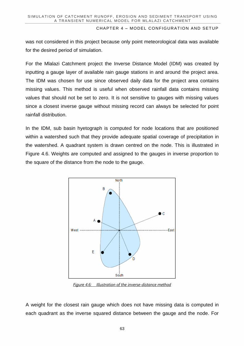
S I MU L A TI O N O F C A TC H ME N T R U N O F F , E R OS I O N A N D S E DI ME N T TR A N S P O R T U S I N G A TR A N S I E N T N U ME R I C A L MO D E L F O R ML A L A Z I C A TC H ME N T
CHAPTER 4 – MODEL CONFIGURATION AND SETUP
63
was not considered in this project because only point meteorological data was available
for the desired period of simulation.
For the Mlalazi Catchment project the Inverse Distance Model (IDM) was created by
inputting a gauge layer of available rain gauge stations in and around the project area.
The IDM was chosen for use since observed daily data for the project area contains
missing values. This method is useful when observed rainfall data contains missing
values that should not be set to zero. It is not sensitive to gauges with missing values
since a closest inverse gauge without missing record can always be selected for point
rainfall distribution.
In the IDM, sub basin hyetograph is computed for node locations that are positioned
within a watershed such that they provide adequate spatial coverage of precipitation in
the watershed. A quadrant system is drawn centred on the node. This is illustrated in
Figure 4.6. Weights are computed and assigned to the gauges in inverse proportion to
the square of the distance from the node to the gauge.
Figure 4.6: Illustration of the inverse-distance method
A weight for the closest rain gauge which does not have missing data is computed in
each quadrant as the inverse squared distance between the gauge and the node. For
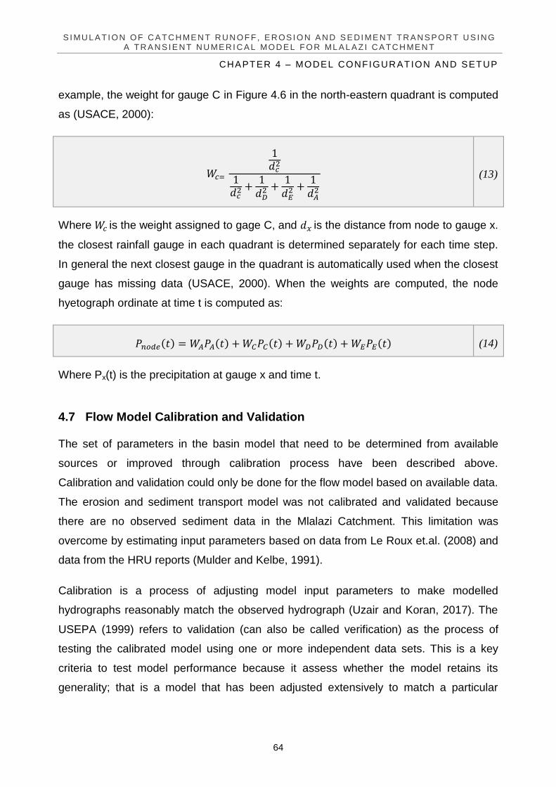
S I MU L A TI O N O F C A TC H ME N T R U N O F F , E R OS I O N A N D S E DI ME N T TR A N S P O R T U S I N G A TR A N S I E N T N U ME R I C A L MO D E L F O R ML A L A Z I C A TC H ME N T
CHAPTER 4 – MODEL CONFIGURATION AND SETUP
64
example, the weight for gauge C in Figure 4.6 in the north-eastern quadrant is computed
as (USACE, 2000):
𝑊𝑐=
1𝑑𝑐
2
1𝑑𝑐
2 +1
𝑑𝐷2 +
1𝑑𝐸
2 +1
𝑑𝐴2
(13)
Where 𝑊𝑐 is the weight assigned to gage C, and 𝑑𝑥 is the distance from node to gauge x.
the closest rainfall gauge in each quadrant is determined separately for each time step.
In general the next closest gauge in the quadrant is automatically used when the closest
gauge has missing data (USACE, 2000). When the weights are computed, the node
hyetograph ordinate at time t is computed as:
𝑃𝑛𝑜𝑑𝑒(𝑡) = 𝑊𝐴𝑃𝐴(𝑡) + 𝑊𝐶𝑃𝐶(𝑡) + 𝑊𝐷𝑃𝐷(𝑡) + 𝑊𝐸𝑃𝐸(𝑡) (14)
Where Px(t) is the precipitation at gauge x and time t.
4.7 Flow Model Calibration and Validation
The set of parameters in the basin model that need to be determined from available
sources or improved through calibration process have been described above.
Calibration and validation could only be done for the flow model based on available data.
The erosion and sediment transport model was not calibrated and validated because
there are no observed sediment data in the Mlalazi Catchment. This limitation was
overcome by estimating input parameters based on data from Le Roux et.al. (2008) and
data from the HRU reports (Mulder and Kelbe, 1991).
Calibration is a process of adjusting model input parameters to make modelled
hydrographs reasonably match the observed hydrograph (Uzair and Koran, 2017). The
USEPA (1999) refers to validation (can also be called verification) as the process of
testing the calibrated model using one or more independent data sets. This is a key
criteria to test model performance because it assess whether the model retains its
generality; that is a model that has been adjusted extensively to match a particular
S I MU L A TI O N O F C A TC H ME N T R U N O F F , E R OS I O N A N D S E DI ME N T TR A N S P O R T U S I N G A TR A N S I E N T N U ME R I C A L MO D E L F O R ML A L A Z I C A TC H ME N T
CHAPTER 4 – MODEL CONFIGURATION AND SETUP
65
events might lose its ability to predict the effects of other events that are not included in
the data used in the calibration process (Uzair and Koran, 2017).
Two approaches are available for simulating hydrological response to meteorological
events that depend on the purpose. Event based model provide an estimate of flow from
the catchment for various extreme types rainfall “events” such as 1:100 year flood.
These events generally operate at short time steps due to the very rapid nature of
changing hydrological conditions. Alternatively, HEC-HMS can simulate long term
“continuous” sequences of flow from a catchment that include these extreme events.
Under these conditions, computational constraints require less stringent time steps.
An event and a continuous based approach were both used in the configuration of the
model. Calibration and validation was done for delineated sub-basins with flow gauging
station W1H012; W1H015; and W1H004 for the runoff model. In order to obtain
reasonably correlation between observed and simulated hydrographs, initial values were
determine, an optimization trial (auto calibration) was run in HEC-HMS and evaluated
using the Nelder and Mead (1965) method. This method used the sum of squared
residuals for the objective function in order to identify the sensitive parameters that were
subsequently manually calibrated.
4.7.1 Event based approach
The main features identified and manually adjusted for event based calibration using
daily observed data running at 6 hour time step to simulate a reasonable hydrographs
were the following:
Peak flow rate;
Time to peak (affected mainly by surface runoff);
Recession curve (represents surface-intermediate-base flow); and
Base flow (represents groundwater/ soil storage that will affect the transport of
sediments between events.
4.7.2 Continuous based approach
The calibration for continuous simulations to determine the rainfall-runoff parameters
was carried out using daily data running at a 1 day time step for the period of 9 years
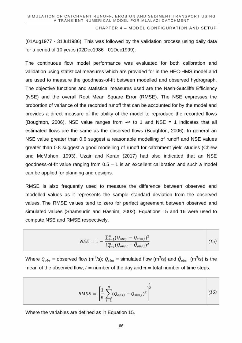
S I MU L A TI O N O F C A TC H ME N T R U N O F F , E R OS I O N A N D S E DI ME N T TR A N S P O R T U S I N G A TR A N S I E N T N U ME R I C A L MO D E L F O R ML A L A Z I C A TC H ME N T
CHAPTER 4 – MODEL CONFIGURATION AND SETUP
66
(01Aug1977 - 31Jul1986). This was followed by the validation process using daily data
for a period of 10 years (02Dec1986 - 01Dec1999).
The continuous flow model performance was evaluated for both calibration and
validation using statistical measures which are provided for in the HEC-HMS model and
are used to measure the goodness-of-fit between modelled and observed hydrograph.
The objective functions and statistical measures used are the Nash-Sutcliffe Efficiency
(NSE) and the overall Root Mean Square Error (RMSE). The NSE expresses the
proportion of variance of the recorded runoff that can be accounted for by the model and
provides a direct measure of the ability of the model to reproduce the recorded flows
(Boughton, 2006). NSE value ranges from -∞ to 1 and NSE = 1 indicates that all
estimated flows are the same as the observed flows (Boughton, 2006). In general an
NSE value greater than 0.6 suggest a reasonable modelling of runoff and NSE values
greater than 0.8 suggest a good modelling of runoff for catchment yield studies (Chiew
and McMahon, 1993). Uzair and Koran (2017) had also indicated that an NSE
goodness-of-fit value ranging from 0.5 – 1 is an excellent calibration and such a model
can be applied for planning and designs.
RMSE is also frequently used to measure the difference between observed and
modelled values as it represents the sample standard deviation from the observed
values. The RMSE values tend to zero for perfect agreement between observed and
simulated values (Shamsudin and Hashim, 2002). Equations 15 and 16 were used to
compute NSE and RMSE respectively.
𝑁𝑆𝐸 = 1 − ∑ (𝑄𝑜𝑏𝑠,𝑖 − 𝑄𝑠𝑖𝑚,𝑖)
2𝑛𝑖=1
∑ (𝑄𝑜𝑏𝑠,𝑖 − �̅�𝑜𝑏𝑠,𝑖)2𝑛𝑖=1
(15)
Where 𝑄𝑜𝑏𝑠 = observed flow (m3/s); 𝑄𝑠𝑖𝑚 = simulated flow (m3/s) and �̅�𝑜𝑏𝑠 (m3/s) is the
mean of the observed flow, 𝑖 = number of the day and 𝑛 = total number of time steps.
𝑅𝑀𝑆𝐸 = [1
𝑛 ∑(𝑄𝑜𝑏𝑠,𝑖 − 𝑄𝑠𝑖𝑚,𝑖)
2
𝑛
𝑖=1
]
12
(16)
Where the variables are defined as in Equation 15.

S I MU L A TI O N O F C A TC H ME N T R U N O F F , E R OS I O N A N D S E DI ME N T TR A N S P O R T U S I N G A TR A N S I E N T N U ME R I C A L MO D E L F O R ML A L A Z I C A TC H ME N T
CHAPTER 5 – RESULTS AND DISCUSSION
67
CHAPTER 5: RESULTS AND DISCUSSION
The results of literature review are presented in Chapter 2 (Literature Review) where the
HEC-HMS was selected as the suitable model to be used for the Mlalazi Catchment.
The result of the creation of the DEM with a required accuracy is presented in Chapter 3
(Study Area and Data), where the geomorphology of the study area is presented after
the DEM was created during the model development stage. Chapter 4 has presented
the model configuration and the selection of process methods of the model. This chapter
will present and discuss the HEC-HMS model flow calibration and validation results, as
well as the continuous simulated catchment flows and sediment load.
5.1 Flow Calibration
5.1.1 Event based Calibration
This event calibration was based on how well the important features of a simulated
storm hydrograph fit the observed hydrograph. The two main features of the model are
the sub-catchment yield and the channel routing that will affect the storm
hydrograph. Both are important in the sediment production and transportation. The
combined yield must correlate closely to the combined runoff for a specific area while
the shape of the hydrograph represents the combined contributions from the storm,
intermediate and base flow components. These are examined for selected conditions
that represent a contribution of a distributed storm events during the monitoring period
between 1984 and 2000.
An event based calibration was done on two selected storm events which could result in
erosion and sediments formations. The simulations were done at a 6 hourly time step for
the station W1H012. The results of the two cyclonic storm events selected for calibration
are shown in Figure 5.1 and Figure 5.2, these were Domoina (31 January 1984) and
Imboa (17 February 1984) respectively. The parameters obtained from the model
calibration are given in Table 5.1.
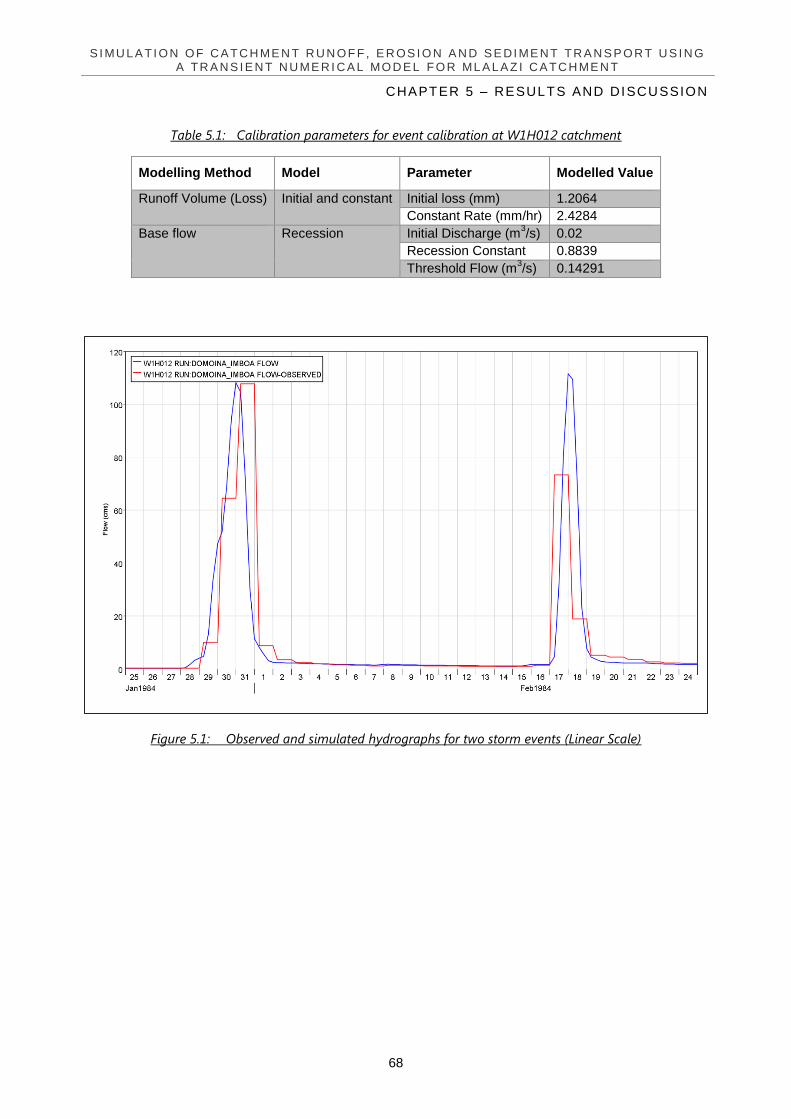
S I MU L A TI O N O F C A TC H ME N T R U N O F F , E R OS I O N A N D S E DI ME N T TR A N S P O R T U S I N G A TR A N S I E N T N U ME R I C A L MO D E L F O R ML A L A Z I C A TC H ME N T
CHAPTER 5 – RESULTS AND DISCUSSION
68
Table 5.1: Calibration parameters for event calibration at W1H012 catchment
Modelling Method Model Parameter Modelled Value
Runoff Volume (Loss) Initial and constant Initial loss (mm) 1.2064
Constant Rate (mm/hr) 2.4284
Base flow Recession Initial Discharge (m3/s) 0.02
Recession Constant 0.8839
Threshold Flow (m3/s) 0.14291
Figure 5.1: Observed and simulated hydrographs for two storm events (Linear Scale)
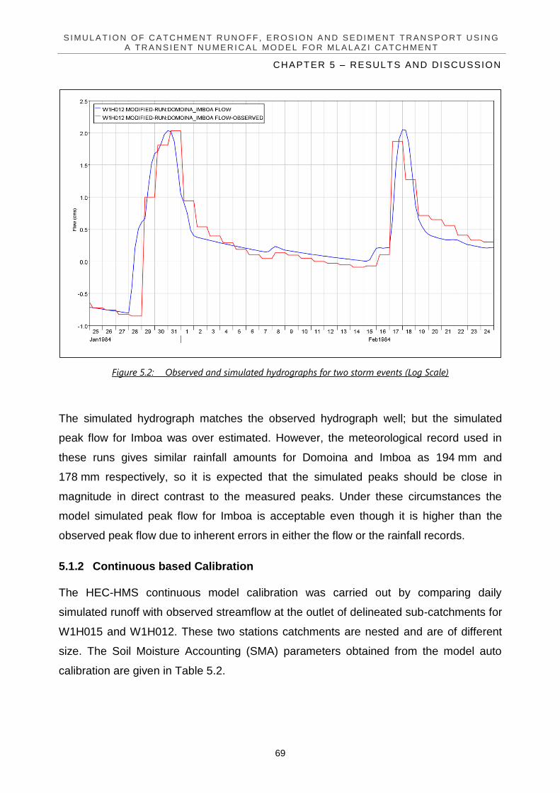
S I MU L A TI O N O F C A TC H ME N T R U N O F F , E R OS I O N A N D S E DI ME N T TR A N S P O R T U S I N G A TR A N S I E N T N U ME R I C A L MO D E L F O R ML A L A Z I C A TC H ME N T
CHAPTER 5 – RESULTS AND DISCUSSION
69
Figure 5.2: Observed and simulated hydrographs for two storm events (Log Scale)
The simulated hydrograph matches the observed hydrograph well; but the simulated
peak flow for Imboa was over estimated. However, the meteorological record used in
these runs gives similar rainfall amounts for Domoina and Imboa as 194 mm and
178 mm respectively, so it is expected that the simulated peaks should be close in
magnitude in direct contrast to the measured peaks. Under these circumstances the
model simulated peak flow for Imboa is acceptable even though it is higher than the
observed peak flow due to inherent errors in either the flow or the rainfall records.
5.1.2 Continuous based Calibration
The HEC-HMS continuous model calibration was carried out by comparing daily
simulated runoff with observed streamflow at the outlet of delineated sub-catchments for
W1H015 and W1H012. These two stations catchments are nested and are of different
size. The Soil Moisture Accounting (SMA) parameters obtained from the model auto
calibration are given in Table 5.2.

S I MU L A TI O N O F C A TC H ME N T R U N O F F , E R OS I O N A N D S E DI ME N T TR A N S P O R T U S I N G A TR A N S I E N T N U ME R I C A L MO D E L F O R ML A L A Z I C A TC H ME N T
CHAPTER 5 – RESULTS AND DISCUSSION
70
Table 5.2: Auto Calibration SMA Parameters for continuous modelling
SMA Parameter Catchment Station
W1H015 W1H012
Max rate of infiltration (mm/hr) 3.3433 4.571322
Soil Storage (mm) 79.193 114.698
Tension Storage (mm) 11.863 13.211826
Soil Percolation (mm/hr) 9.6467 4.9952
GW 1 Storage (mm) 50.095 4.11523
GW 1 percolation (mm/hr) 12.777 13.88954
GW 1 coefficient (hr) 27.125 39.41356
GW 2 Storage (mm) 93.542 72.63342
GW 2 percolation (mm/hr) 7.2213 5.943966
GW 2 coefficient (hr) 89.527 151.39457
The simulate NSE for the calibration for W1H015 is 0.71, and 0.78 for W1H012. These
NSE values obtained suggest a good result for calibration of runoff; the ranges of NSE
are discussed in detailed in the earlier Chapter 4. The simulated RMSE of calibration for
W1H015 was 0.3 m3/s and 1.4 m3/s for W1H012. The RMSE for the calibration period
tend to be reasonably close to zero for station W1H015 and for W1H012 it was
reasonable. These results obtained are considered satisfactory and acceptable for runoff
simulations.
The study area is characterised by unreliable rainfall data and observed streamflow data
with missing records, and prone to errors especially at high flows, that could have
affected the NSE and RMSE values for the continuous based calibration. The RMSE
and NSE values obtained from calibration results are shown in Table 5.3 below.
Table 5.3: Performance measures of the model
Gauge Catchment Error function Calibration Period
W1H015 NSE 0.71
RMSE 0.3 (m3/s)
W1H012 NSE 0.78
RMSE 1.4 (m3/s)

S I MU L A TI O N O F C A TC H ME N T R U N O F F , E R OS I O N A N D S E DI ME N T TR A N S P O R T U S I N G A TR A N S I E N T N U ME R I C A L MO D E L F O R ML A L A Z I C A TC H ME N T
CHAPTER 5 – RESULTS AND DISCUSSION
71
The calibration period simulated runoff and their comparison to observed stream flow on
a log scale for stations W1H015 and W1H012 are given in Figure 5.3 and Figure 5.5,
and the cumulative yield for the same period in Figure 5.4 and Figure 5.6 respectively.
For description of the plots, the yellow is the missing data symbol; the red line is
observed data, while the simulated data is always presented by a blue line in all the
result plots.

SIMULATION OF CATCHMENT RUNOFF, EROSION AND SEDIMENT TRANSPORT USING A TRANSIENT NUMERICAL MODEL FOR MLALAZI CATCHMENT
CHAPTER 5 – RESULTS AND DISCUSSION
72
Figure 5.3: W1H015 Observed and simulated streamflow (Log Scale) Figure 5.4: W1H015 Cumulative observed and simulated streamflow
Figure 5.5: W1H012 Observed and simulated streamflow (Log Scale) Figure 5.6: W1H012 Cumulative observed and simulated streamflow
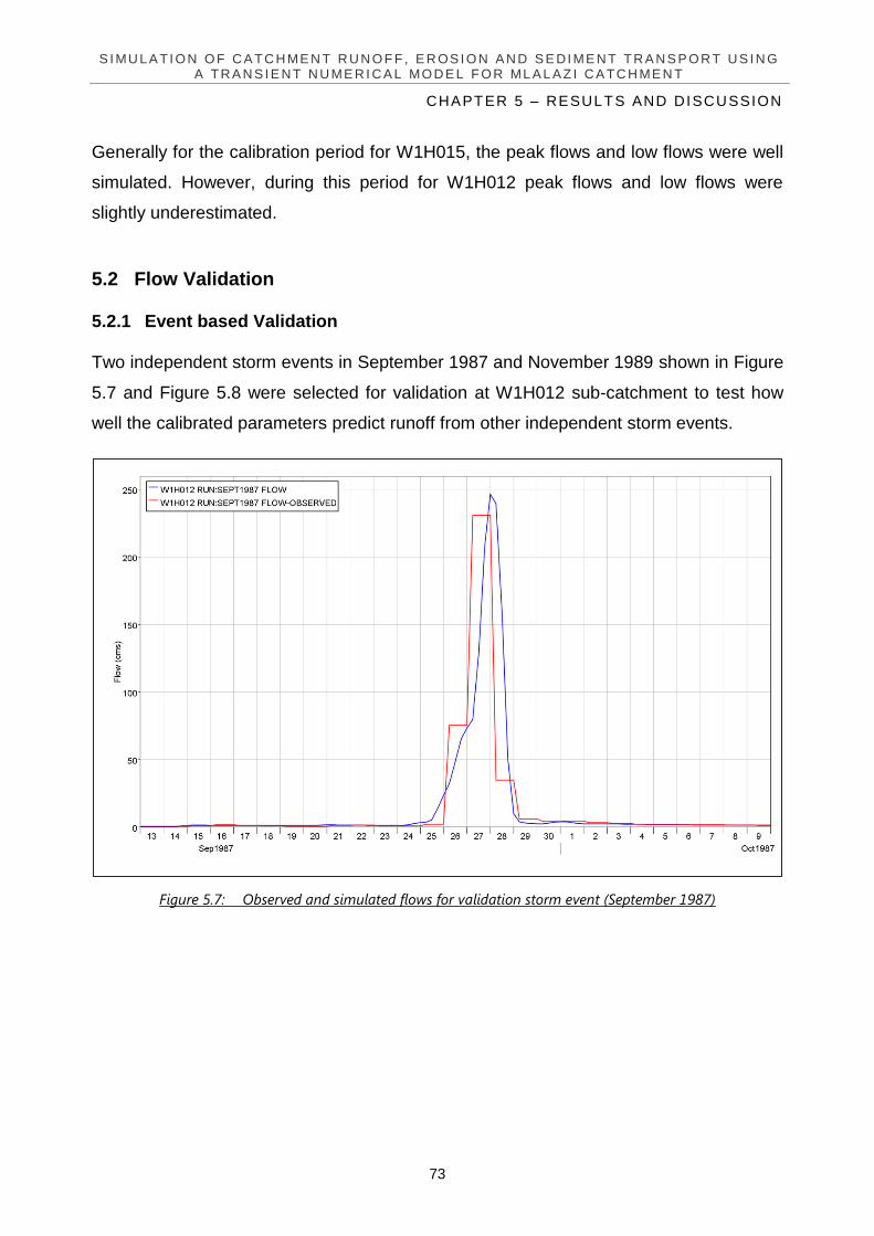
S I MU L A TI O N O F C A TC H ME N T R U N O F F , E R OS I O N A N D S E DI ME N T TR A N S P O R T U S I N G A TR A N S I E N T N U ME R I C A L MO D E L F O R ML A L A Z I C A TC H ME N T
CHAPTER 5 – RESULTS AND DISCUSSION
73
Generally for the calibration period for W1H015, the peak flows and low flows were well
simulated. However, during this period for W1H012 peak flows and low flows were
slightly underestimated.
5.2 Flow Validation
5.2.1 Event based Validation
Two independent storm events in September 1987 and November 1989 shown in Figure
5.7 and Figure 5.8 were selected for validation at W1H012 sub-catchment to test how
well the calibrated parameters predict runoff from other independent storm events.
Figure 5.7: Observed and simulated flows for validation storm event (September 1987)

S I MU L A TI O N O F C A TC H ME N T R U N O F F , E R OS I O N A N D S E DI ME N T TR A N S P O R T U S I N G A TR A N S I E N T N U ME R I C A L MO D E L F O R ML A L A Z I C A TC H ME N T
CHAPTER 5 – RESULTS AND DISCUSSION
74
Figure 5.8: Observed and simulated flows for validation storm event (November 1989)
Both simulated storm events show good agreement between the predicted and
observed storm hydrographs. However, the November 1989 peaked early than the
observed hydrograph. This possibly is because of the difference in time steps, where the
simulation was for a 6 hour time step and the observed data was daily.
5.2.2 Continuous based Validation
The simulated NSE for the validation period for station W1H015 was 0.62 and the RMSE
was 0.4 m3/s. The NSE for W1H012 was also 0.62, while the RMSE was 2.8 m3/s (Table
5.4). The results obtained for the validation period are satisfactory and considered
acceptable for rainfall-runoff simulations based on the condition that the NSE is greater
than 0.6 that is a good model performance, and the RMSE of 2.8 m3/s is reasonable
although not the closest to zero.
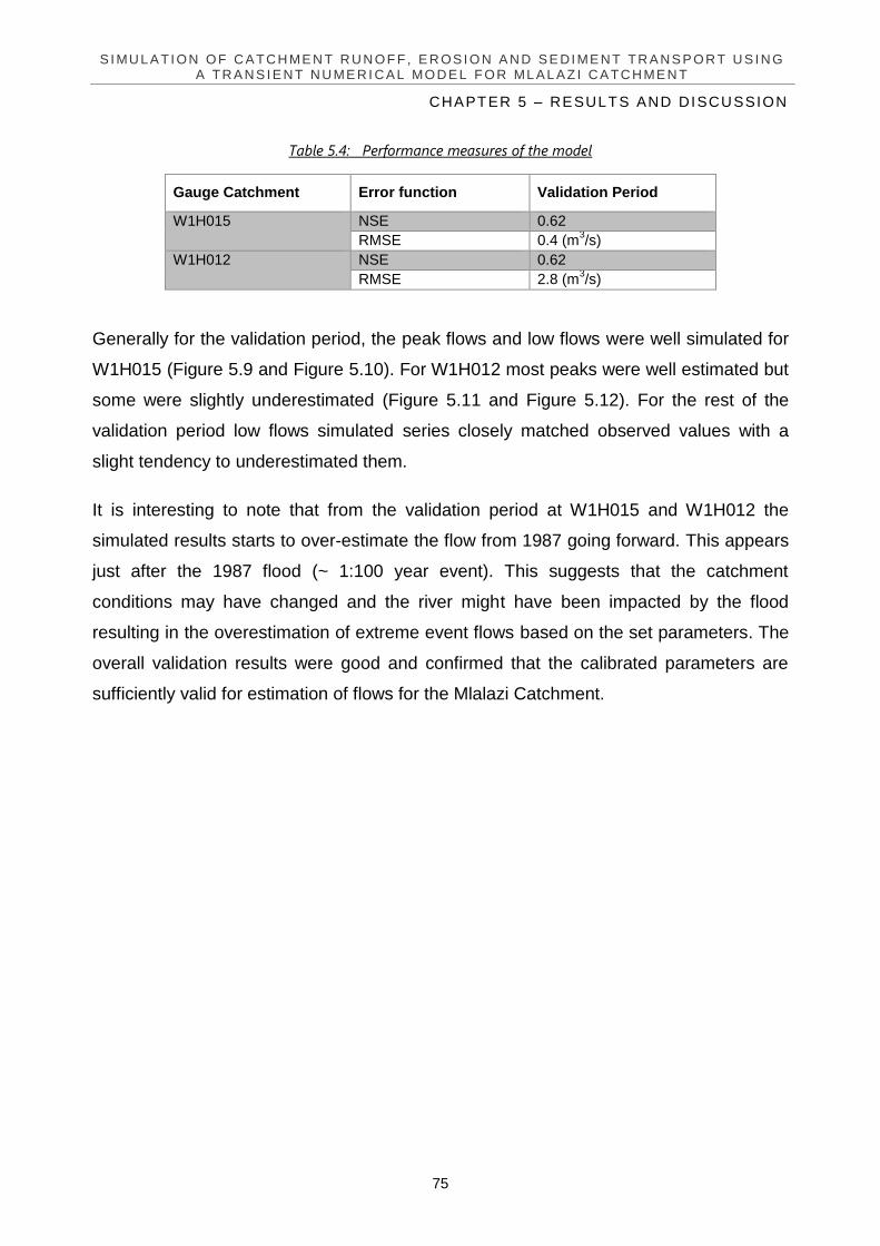
S I MU L A TI O N O F C A TC H ME N T R U N O F F , E R OS I O N A N D S E DI ME N T TR A N S P O R T U S I N G A TR A N S I E N T N U ME R I C A L MO D E L F O R ML A L A Z I C A TC H ME N T
CHAPTER 5 – RESULTS AND DISCUSSION
75
Table 5.4: Performance measures of the model
Gauge Catchment Error function Validation Period
W1H015 NSE 0.62
RMSE 0.4 (m3/s)
W1H012 NSE 0.62
RMSE 2.8 (m3/s)
Generally for the validation period, the peak flows and low flows were well simulated for
W1H015 (Figure 5.9 and Figure 5.10). For W1H012 most peaks were well estimated but
some were slightly underestimated (Figure 5.11 and Figure 5.12). For the rest of the
validation period low flows simulated series closely matched observed values with a
slight tendency to underestimated them.
It is interesting to note that from the validation period at W1H015 and W1H012 the
simulated results starts to over-estimate the flow from 1987 going forward. This appears
just after the 1987 flood (~ 1:100 year event). This suggests that the catchment
conditions may have changed and the river might have been impacted by the flood
resulting in the overestimation of extreme event flows based on the set parameters. The
overall validation results were good and confirmed that the calibrated parameters are
sufficiently valid for estimation of flows for the Mlalazi Catchment.
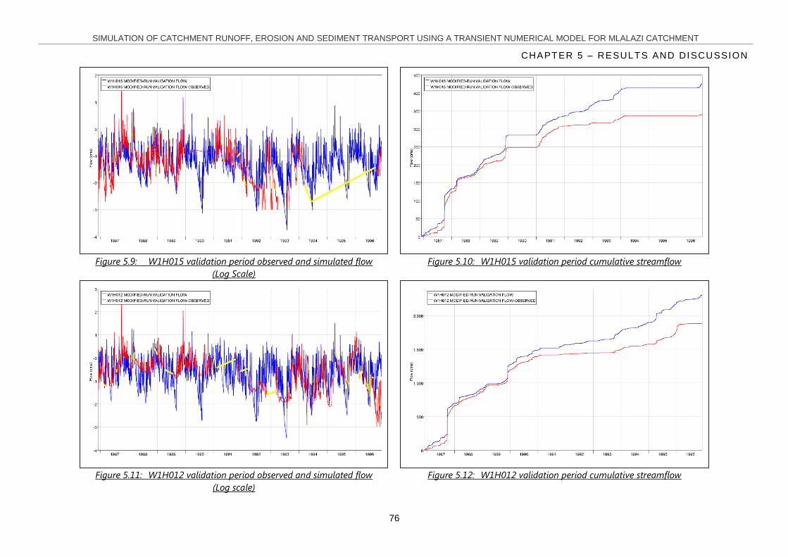
SIMULATION OF CATCHMENT RUNOFF, EROSION AND SEDIMENT TRANSPORT USING A TRANSIENT NUMERICAL MODEL FOR MLALAZI CATCHMENT
CHAPTER 5 – RESULTS AND DISCUSSION
76
Figure 5.9: W1H015 validation period observed and simulated flow
(Log Scale)
Figure 5.10: W1H015 validation period cumulative streamflow
Figure 5.11: W1H012 validation period observed and simulated flow
(Log scale)
Figure 5.12: W1H012 validation period cumulative streamflow
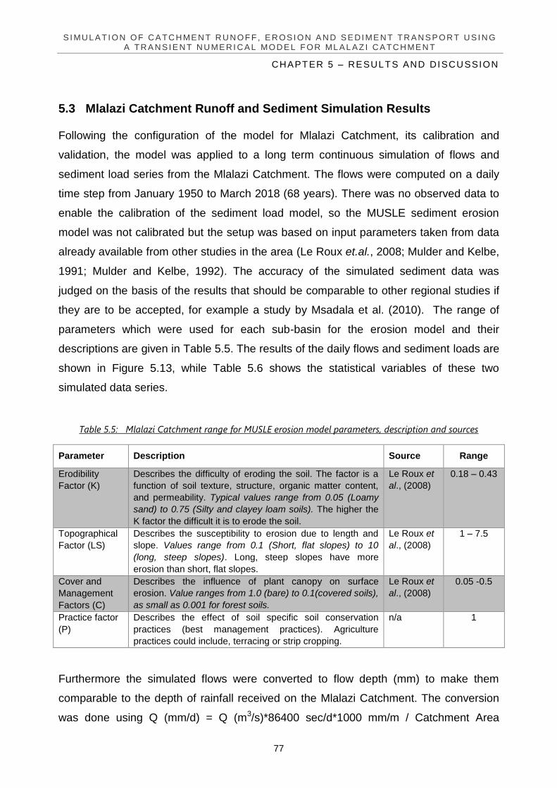
S I MU L A TI O N O F C A TC H ME N T R U N O F F , E R OS I O N A N D S E DI ME N T TR A N S P O R T U S I N G A TR A N S I E N T N U ME R I C A L MO D E L F O R ML A L A Z I C A TC H ME N T
CHAPTER 5 – RESULTS AND DISCUSSION
77
5.3 Mlalazi Catchment Runoff and Sediment Simulation Results
Following the configuration of the model for Mlalazi Catchment, its calibration and
validation, the model was applied to a long term continuous simulation of flows and
sediment load series from the Mlalazi Catchment. The flows were computed on a daily
time step from January 1950 to March 2018 (68 years). There was no observed data to
enable the calibration of the sediment load model, so the MUSLE sediment erosion
model was not calibrated but the setup was based on input parameters taken from data
already available from other studies in the area (Le Roux et.al., 2008; Mulder and Kelbe,
1991; Mulder and Kelbe, 1992). The accuracy of the simulated sediment data was
judged on the basis of the results that should be comparable to other regional studies if
they are to be accepted, for example a study by Msadala et al. (2010). The range of
parameters which were used for each sub-basin for the erosion model and their
descriptions are given in Table 5.5. The results of the daily flows and sediment loads are
shown in Figure 5.13, while Table 5.6 shows the statistical variables of these two
simulated data series.
Table 5.5: Mlalazi Catchment range for MUSLE erosion model parameters, description and sources
Parameter Description Source Range
Erodibility
Factor (K)
Describes the difficulty of eroding the soil. The factor is a
function of soil texture, structure, organic matter content,
and permeability. Typical values range from 0.05 (Loamy
sand) to 0.75 (Silty and clayey loam soils). The higher the
K factor the difficult it is to erode the soil.
Le Roux et
al., (2008)
0.18 – 0.43
Topographical
Factor (LS)
Describes the susceptibility to erosion due to length and
slope. Values range from 0.1 (Short, flat slopes) to 10
(long, steep slopes). Long, steep slopes have more
erosion than short, flat slopes.
Le Roux et
al., (2008)
1 – 7.5
Cover and
Management
Factors (C)
Describes the influence of plant canopy on surface
erosion. Value ranges from 1.0 (bare) to 0.1(covered soils),
as small as 0.001 for forest soils.
Le Roux et
al., (2008)
0.05 -0.5
Practice factor
(P)
Describes the effect of soil specific soil conservation
practices (best management practices). Agriculture
practices could include, terracing or strip cropping.
n/a 1
Furthermore the simulated flows were converted to flow depth (mm) to make them
comparable to the depth of rainfall received on the Mlalazi Catchment. The conversion
was done using Q (mm/d) = Q (m3/s)*86400 sec/d*1000 mm/m / Catchment Area

S I MU L A TI O N O F C A TC H ME N T R U N O F F , E R OS I O N A N D S E DI ME N T TR A N S P O R T U S I N G A TR A N S I E N T N U ME R I C A L MO D E L F O R ML A L A Z I C A TC H ME N T
CHAPTER 5 – RESULTS AND DISCUSSION
78
(397 000 000 m2). The plot of three rainfall stations used and the simulated runoff in mm
depth for the same period is given in Figure 5.14.
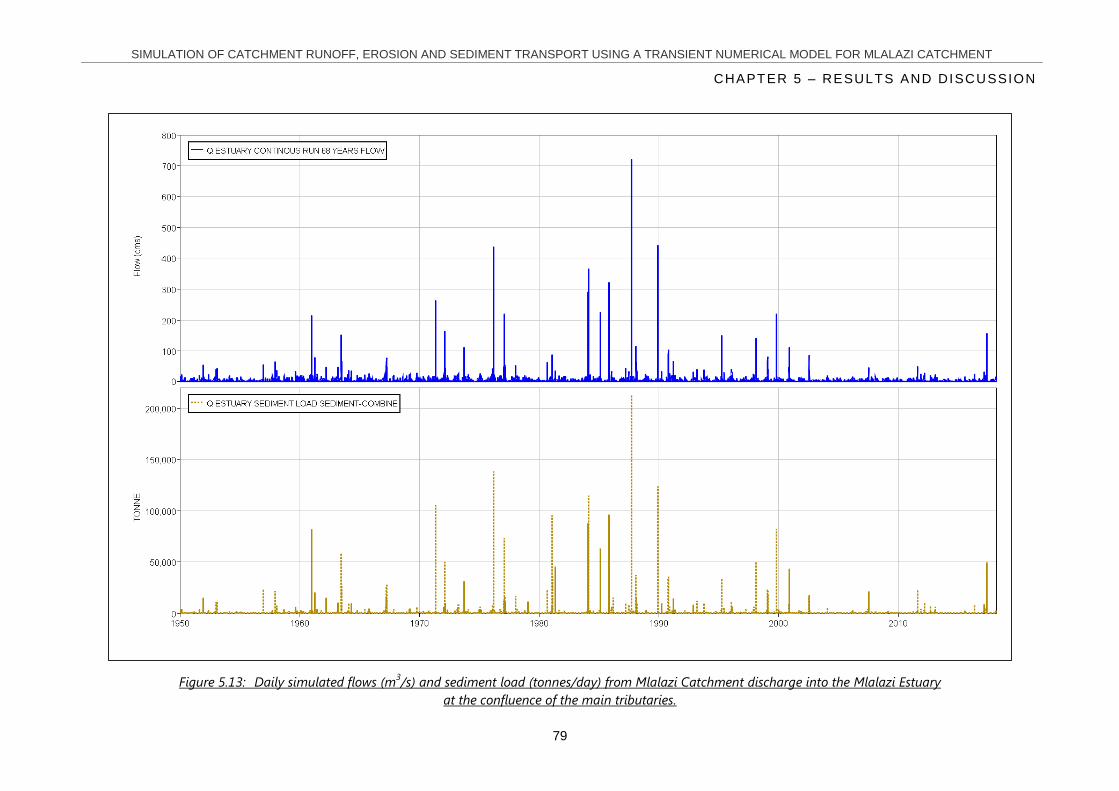
SIMULATION OF CATCHMENT RUNOFF, EROSION AND SEDIMENT TRANSPORT USING A TRANSIENT NUMERICAL MODEL FOR MLALAZI CATCHMENT
CHAPTER 5 – RESULTS AND DISCUSSION
79
Figure 5.13: Daily simulated flows (m3/s) and sediment load (tonnes/day) from Mlalazi Catchment discharge into the Mlalazi Estuary
at the confluence of the main tributaries.

SIMULATION OF CATCHMENT RUNOFF, EROSION AND SEDIMENT TRANSPORT USING A TRANSIENT NUMERICAL MODEL FOR MLALAZI CATCHMENT
CHAPTER 5 – RESULTS AND DISCUSSION
80
Figure 5.14: Simulated flow depth (mm/day) and Rainfall (mm/day)

S I MU L A TI O N O F C A TC H ME N T R U N O F F , E R OS I O N A N D S E DI ME N T TR A N S P O R T U S I N G A TR A N S I E N T N U ME R I C A L MO D E L F O R ML A L A Z I C A TC H ME N T
CHAPTER 5 – RESULTS AND DISCUSSION
81
Table 5.6: Statistical variables of simulated flows and sediment load
Statistical Variable Daily simulated Flows (m3/s) Daily simulated Sediment Load (tonne)
Minimum Value 2.69 * 10-4
2.92 * 10-26
Mean Value 2.76 207.61
Maximum Value 720.11 212772.31
Standard Deviation 11.64 3258.32
Skew Coeffcient 29.37 34.49
The most extreme event experienced during the period of simulation was in 1987
wherein a daily rainfall amount between 260 mm and 350 mm that was recorded for this
catchment produced a runoff of approximately 150 mm in depth. This event has also
yielded a sediment load of approximately 210 000 tonnes per day.
From Figure 5.14 presented above, it can be noted that the rainfall data series from
2000 to the end of the simulation period has shown a significant difference, with W13A
showing less rainfall records compared to Port Durnford. This has sigficantly affected the
resultant simulated runoff and sediment yield from the catchment. This period fell
outside the monitoring period for most of the surrounding stations, which meant that the
derivation of centroid station W13A rainfall data series was dependent on only one
station which was Eshowe Municipality. This is a manual station which could have been
subjected to various errors and there was no luxury for comparison with records from
other stations and/or the filling of suspected data. It is also believed that after 2006 the
quality control over data from SAWS was stopped.
A frequency analysis plot shown in Figure 5.15 was computed in HEC-DSS for the
simulated daily flows. This was to be able to identify the reccurrence intervals of different
peak discharges out of the catchment as a resultant of rainfall extreme events.
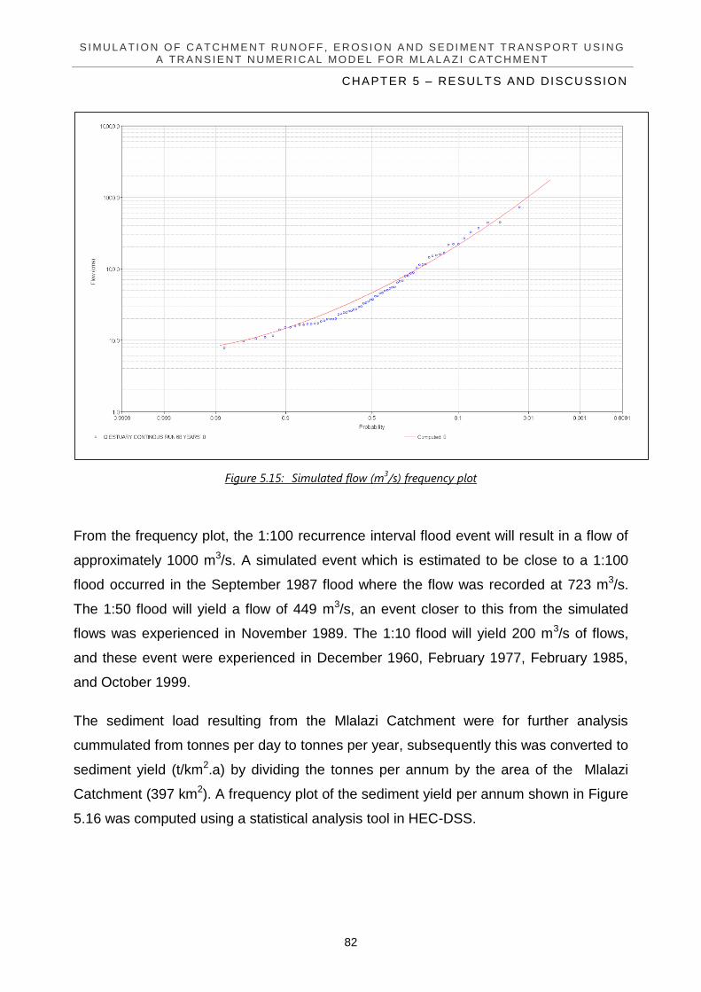
S I MU L A TI O N O F C A TC H ME N T R U N O F F , E R OS I O N A N D S E DI ME N T TR A N S P O R T U S I N G A TR A N S I E N T N U ME R I C A L MO D E L F O R ML A L A Z I C A TC H ME N T
CHAPTER 5 – RESULTS AND DISCUSSION
82
Figure 5.15: Simulated flow (m3/s) frequency plot
From the frequency plot, the 1:100 recurrence interval flood event will result in a flow of
approximately 1000 m3/s. A simulated event which is estimated to be close to a 1:100
flood occurred in the September 1987 flood where the flow was recorded at 723 m3/s.
The 1:50 flood will yield a flow of 449 m3/s, an event closer to this from the simulated
flows was experienced in November 1989. The 1:10 flood will yield 200 m3/s of flows,
and these event were experienced in December 1960, February 1977, February 1985,
and October 1999.
The sediment load resulting from the Mlalazi Catchment were for further analysis
cummulated from tonnes per day to tonnes per year, subsequently this was converted to
sediment yield (t/km2.a) by dividing the tonnes per annum by the area of the Mlalazi
Catchment (397 km2). A frequency plot of the sediment yield per annum shown in Figure
5.16 was computed using a statistical analysis tool in HEC-DSS.
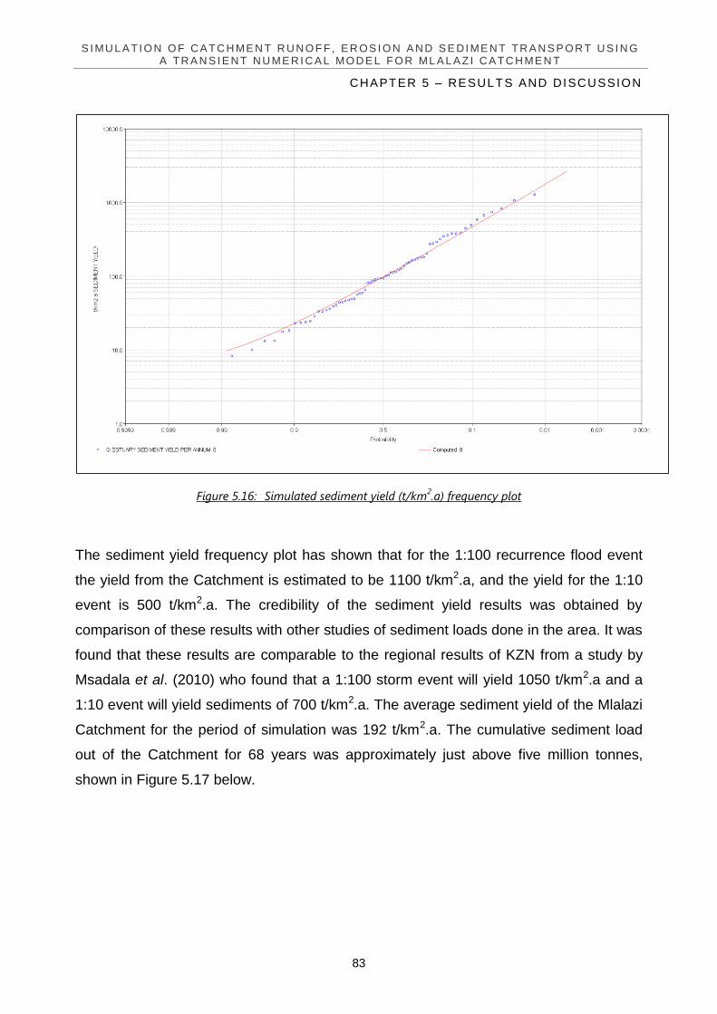
S I MU L A TI O N O F C A TC H ME N T R U N O F F , E R OS I O N A N D S E DI ME N T TR A N S P O R T U S I N G A TR A N S I E N T N U ME R I C A L MO D E L F O R ML A L A Z I C A TC H ME N T
CHAPTER 5 – RESULTS AND DISCUSSION
83
Figure 5.16: Simulated sediment yield (t/km2.a) frequency plot
The sediment yield frequency plot has shown that for the 1:100 recurrence flood event
the yield from the Catchment is estimated to be 1100 t/km2.a, and the yield for the 1:10
event is 500 t/km2.a. The credibility of the sediment yield results was obtained by
comparison of these results with other studies of sediment loads done in the area. It was
found that these results are comparable to the regional results of KZN from a study by
Msadala et al. (2010) who found that a 1:100 storm event will yield 1050 t/km2.a and a
1:10 event will yield sediments of 700 t/km2.a. The average sediment yield of the Mlalazi
Catchment for the period of simulation was 192 t/km2.a. The cumulative sediment load
out of the Catchment for 68 years was approximately just above five million tonnes,
shown in Figure 5.17 below.
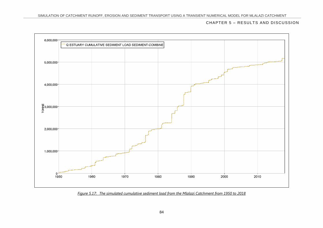
SIMULATION OF CATCHMENT RUNOFF, EROSION AND SEDIMENT TRANSPORT USING A TRANSIENT NUMERICAL MODEL FOR MLALAZI CATCHMENT
CHAPTER 5 – RESULTS AND DISCUSSION
84
Figure 5.17: The simulated cumulative sediment load from the Mlalazi Catchment from 1950 to 2018

S I MU L A TI O N O F C A TC H ME N T R U N O F F , E R OS I O N A N D S E DI ME N T TR A N S P O R T U S I N G A TR A N S I E N T N U ME R I C A L MO D E L F O R ML A L A Z I C A TC H ME N T
CHAPTER 5 – RESULTS AND DISCUSSION
85
In order to establish information of sediment grainsize distribution along the two main
tributaries (Mlalazi and Ntuze River) and erosion from different land use sections,
sediment yield data were further analysed and presented based on grain sizes (sand,
gravel, silt and clay). This was achieved by dividing the sediment load per day (tonnes)
by the catchment area contributing to the point selected, to result in tonnes per day per
square kilometre of area (SQKM). The grain sizes results presented below are for the
following areas: W1H004 catchment (Figure 5.18); W1H012 station which covers much
of the Ntuze River tributary catchment (Figure 5.19) and a point on Mlalazi River before
confluence with Ntuze River (Figure 5.20).
Figure 5.18: W1H004 Catchment simulated sediment grain size distribution (tonnes/day.km2)
The catchment of station W1H004 which its sediment yield as a result of erosion is
presented above is a catchment dominated by a land use of commercial sugarcane
plantation. Results have showed that the sediments produced are constituted by mostly
sand and gravel. During the 1:100 year flood event experience in September 1987 this
catchment produced a daily sediment yield of approximately 4.6 tonnes per square km
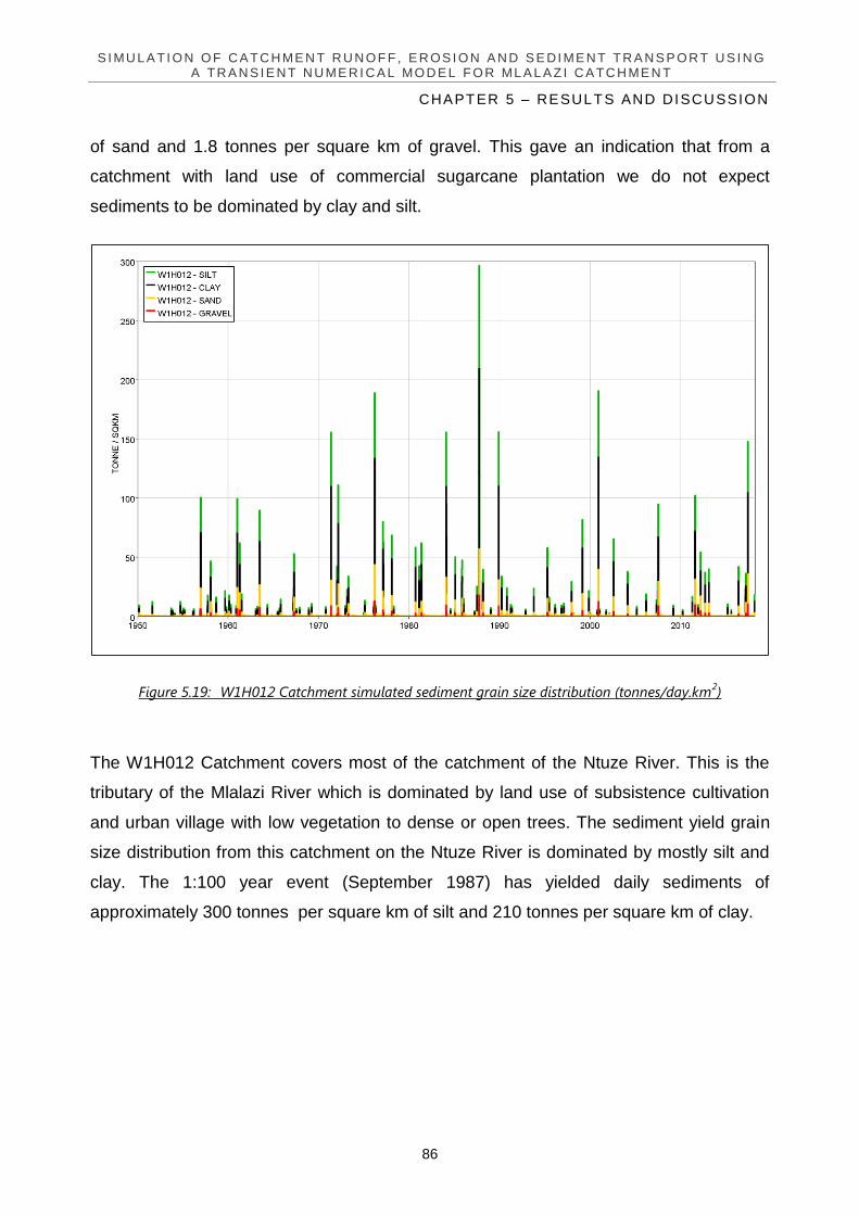
S I MU L A TI O N O F C A TC H ME N T R U N O F F , E R OS I O N A N D S E DI ME N T TR A N S P O R T U S I N G A TR A N S I E N T N U ME R I C A L MO D E L F O R ML A L A Z I C A TC H ME N T
CHAPTER 5 – RESULTS AND DISCUSSION
86
of sand and 1.8 tonnes per square km of gravel. This gave an indication that from a
catchment with land use of commercial sugarcane plantation we do not expect
sediments to be dominated by clay and silt.
Figure 5.19: W1H012 Catchment simulated sediment grain size distribution (tonnes/day.km2)
The W1H012 Catchment covers most of the catchment of the Ntuze River. This is the
tributary of the Mlalazi River which is dominated by land use of subsistence cultivation
and urban village with low vegetation to dense or open trees. The sediment yield grain
size distribution from this catchment on the Ntuze River is dominated by mostly silt and
clay. The 1:100 year event (September 1987) has yielded daily sediments of
approximately 300 tonnes per square km of silt and 210 tonnes per square km of clay.
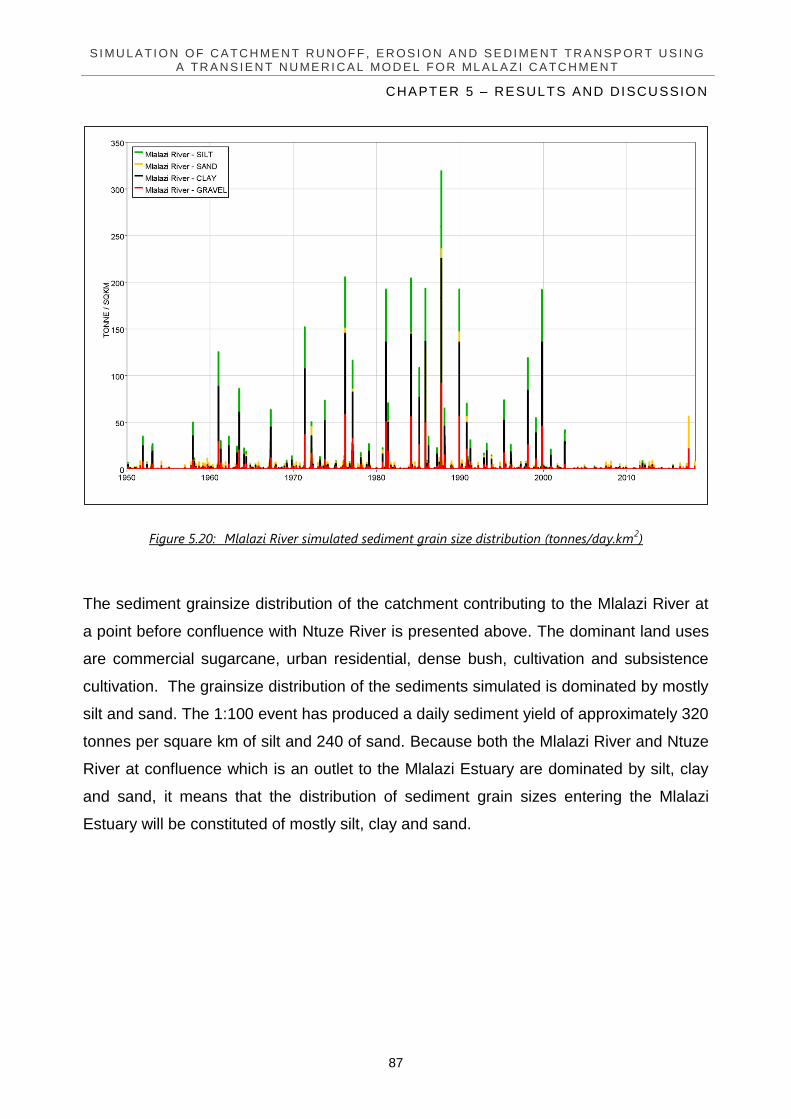
S I MU L A TI O N O F C A TC H ME N T R U N O F F , E R OS I O N A N D S E DI ME N T TR A N S P O R T U S I N G A TR A N S I E N T N U ME R I C A L MO D E L F O R ML A L A Z I C A TC H ME N T
CHAPTER 5 – RESULTS AND DISCUSSION
87
Figure 5.20: Mlalazi River simulated sediment grain size distribution (tonnes/day.km2)
The sediment grainsize distribution of the catchment contributing to the Mlalazi River at
a point before confluence with Ntuze River is presented above. The dominant land uses
are commercial sugarcane, urban residential, dense bush, cultivation and subsistence
cultivation. The grainsize distribution of the sediments simulated is dominated by mostly
silt and sand. The 1:100 event has produced a daily sediment yield of approximately 320
tonnes per square km of silt and 240 of sand. Because both the Mlalazi River and Ntuze
River at confluence which is an outlet to the Mlalazi Estuary are dominated by silt, clay
and sand, it means that the distribution of sediment grain sizes entering the Mlalazi
Estuary will be constituted of mostly silt, clay and sand.

S I MU L A TI O N O F C A TC H ME N T R U N O F F , E R OS I O N A N D S E DI ME N T TR A N S P O R T U S I N G A TR A N S I E N T N U ME R I C A L MO D E L F O R ML A L A Z I C A TC H ME N T
CHAPTER 6 – CONCLUSIONS AND RECOMMENDATIONS
88
CHAPTER 6: CONCLUSIONS AND
RECOMMENDATIONS
The Mlalazi Estuary is prone to degradation from changing fluvial processes which will
result in increased sediment yields from the catchment into the estuary; this could lead
to management interventions such as mechanical breaching of the mouth to remove the
sediments. This however, will need to be an objective decision to be made as opposed
to a subjective one, based on the best available information. In the interest of objectivity
in decision making, a need arises to assess the catchment and estuary systems using
the best information that is frequently derived from numerical models which provide
results that are comparable, reproducible and enable the prediction of effects from
causes. It is for this reason that the HRU – University of Zululand is conducting a study
funded by the WRC which aims at deriving hydrodynamic information of the Mlalazi
Estuary which will assist in decision making and be applicable in other estuaries of
similar hydrological conditions such as the Siyaya Estuary which is has been closed for
an extended period of time. The necessity for that study was also because the Mlalazi
Estuary’s Rapid Ecological Water Reserve (EWR) study by DWS (2015) was based on
low confidence simulated monthly flows and no sediment information. This illustrated
that there is no daily or sub-daily flow and sediment data for the Mlalazi Catchment
which could be used to derive estuary hydrodynamic information. The EWR study was
aimed at assisting DWS in making informed decisions regarding the authorisations of
future water use and the magnitude of the impacts of the proposed developments on the
water resources in the catchment, and to provide the input data for classification of the
areas of the water resources.
The aim of this study was, as part of the study by the HRU, to derive reliable best
estimates of the flows and sediments load out of the Mlalazi Catchment which is to be
routed to the estuary catchment. This is because flows, erosion and sediment transport
are the main drivers which may impact the opening and the closing of the estuary
mouth. Given that these data is not measured for the Mlalazi Catchment as a whole, the
hypothesis tested was that a physically based, numerical simulation model is the most
S I MU L A TI O N O F C A TC H ME N T R U N O F F , E R OS I O N A N D S E DI ME N T TR A N S P O R T U S I N G A TR A N S I E N T N U ME R I C A L MO D E L F O R ML A L A Z I C A TC H ME N T
CHAPTER 6 – CONCLUSIONS AND RECOMMENDATIONS
89
pragmatic tool for the derivation of hydrodynamic information in catchments with limited
observed data.
A literature reviewed of MIKE SHE, ACRU, SHETRAN, HEC-HMS and SWAT as
suitable models with the capacity to achieve the required results was conducted for the
purpose of this study to select a suitable model for application in the Mlalazi catchment.
The MIKE SHE and SHETRAN could not be used because they are commercial
products that were not freely available. The ACRU model although being an open
source was not selected because it does not allow the routing of sediments. SWAT has
data intensive requirements that were not available for the catchment. The HEC-HMS
model was selected as the preferred model because it allowed some hydrological
processes to be simulated using empirical or parameter fitting process models, rather
than using mostly physical sub-models which will require measured data which might not
be available for Mlalazi Catchment.
The Mlalazi Catchment is characterised by rainfall records that were not reliable and not
always consistent with streamflows. This study had a limited series of observed flow
data that did not cover the catchment adequately. However, this was overcome by using
delineated sub-catchments for stations with data on the Ntuze Catchment for calibration.
The results were extrapolated to other sub-catchments which are not gauged but have
similar catchment characteristics. It was critical in this study to analyse the accuracy of
the flow data used for calibration, this was because the rainfall data and streamflow data
did not always correspond to one another, especially for extreme events. The flow
gauging station W1H012 mostly used for calibration and validation was overestimating
flows for extreme events which made it difficult to calibrate the model successfully. This
was overcome by using a fitted equation discharge table produced from current gauging
and slope area method to calibrate and validate the model. It was a lesson learnt that
because a discharge table is a theoretical relationship, it can be prone to errors
especially at high flows which could be due to submergence effect and as a result a
flood event could be overestimated. This suggests that after any flood event, it is
important that the flood marks are surveyed in order to determine the magnitude of the
flood event accurately.
S I MU L A TI O N O F C A TC H ME N T R U N O F F , E R OS I O N A N D S E DI ME N T TR A N S P O R T U S I N G A TR A N S I E N T N U ME R I C A L MO D E L F O R ML A L A Z I C A TC H ME N T
CHAPTER 6 – CONCLUSIONS AND RECOMMENDATIONS
90
The HEC-HMS model was configured in HEC-GeoHMS and setup. A hydrologically
correct and depressionless DEM derived formed the basis of the derivation of all
geospatial and input files into HEC-HMS Model. Since HEC-HMS is a semi-distributed
model, sub-basins were divided based on similar land use and location of flow gauges
which allowed for input data to be lumped for some catchments. An event based and a
continuous based approach for model calibration has allowed a configuration of a model
would be able to simulate other storm events in future. The overall results of the
calibration and validation of the continuous simulations were good and confirmed that
the calibrated parameters are sufficiently valid for estimation of flows for the Mlalazi
Catchment. The flows were then computed on a daily time step from January 1950 to
March 2018 (68 years) for use in the study by the HRU.
There was no observed data to enable the calibration of the sediment yield model, so
the MUSLE sediment model was not calibrated but was setup based on input
parameters taken from data already available from other studies in the area. The
accuracy of the simulated sediment data was evaluated on the basis that the results
should be comparable to other regional studies. The sediment yield simulations have
shown that for a 1:100 recurrence flood event the yield from the catchment is 1100
t/km2.a, the yield for the 1:10 event is 500 t/km2.a. It was found that the sediment results
are comparable to the regional study by Msadala et al. (2010) who found that a 1:100
storm event will yielded 1050 t/km2.a and a 1:10 event yielded sediments of 700 t/km2.a.
This study of Mlalazi Catchment has found that the distribution of sediment grain sizes
entering the Mlalazi Estuary will be constituted of mostly silt, clay and sand respectively.
It was concluded that the use a calibrated HEC-HMS model in the Mlalazi Catchment
which is characterised by limited observed data was the most pragmatic approach to
derive the best estimates of the flows and sediment yield information for the Mlalazi
Catchment, information that was lacking in the EWR (2015) study. If the Hydrological
Research Unit (HRU) of the University of Zululand is to be reinstituted, it is
recommended that the flow gauge W1H012 should be resurrected since it has proven to
be crucial for catchment studies. It is also recommended that the DWS as part of its
monitoring network should consider monitoring sites for sediment load in the Mlalazi
Catchment since this data is not monitored for the catchment as a whole. This is
because the sediment transport is also one of the drivers of the estuary dynamics.
S I MU L A TI O N O F C A TC H ME N T R U N O F F , E R OS I O N A N D S E DI ME N T TR A N S P O R T U S I N G A TR A N S I E N T N U ME R I C A L MO D E L F O R ML A L A Z I C A TC H ME N T
REFERENCES
91
REFERENCES
Abbott, M.B., Bathurst, J.C., Cunge, J.A., O'Connell, P.E., and Rasmussen, J. (1986) An introduction
to the European Hydrological System - Système Hydrologique Européen, SHE, 2: Structure
of a physically-based, distributed modelling system. J. Hydrol., 87, 6177.
Andersen, J., Refsgaard, J.C. and Jensen, K.H. (2001) Distributed hydrological modelling of the
Senegal River Basin – model construction and validation. Journal of hydrology, 247: 200–
214.
ARC-ISCW Staff. (2004) Generalised soil patterns of South Africa. (2004). ARC-ISCW, Pretoria.
Arnold, J.G., Muttiahb, R.S., Srinivasan, R. and Alen P.M. (2000). Regional estimation of base flow
and groundwater recharge in the upper Mississippi River basin. Journal of Hydrology, 227,
21-40.
Beck, J.S. and Basson, G.R. (2008) Klein River Estuary (South Africa): 2D numerical modelling of
estuary breaching. Water SA Vol. 34
Begg, G.W. (1978) The estuaries of Natal. Natal Town and Regional Planning Commission.
Pietermaritzburg.
Bennett, J.P. (1974) Concepts of mathematical modelling of sediment yield. Water Resources
Research 10, 485–492.
Bennett, T.H. (1998) Development and application of a continuous soil moisture accounting algorithm
of the HEC-HMS. MSc thesis, department of civil and environmental engineering, University
of California, Davis.
Beven, K. J. (2001) Rainfall-Runoff modeling: The Primer, John Wiley and Sons Ltd, England. pp
372.
Boughton, W.C. (2006) Calibrations of a daily rainfall–runoff model with poor quality data.
Environmental Modelling and Software Journal 21, 1114–1128.
Butts, M.B., Payne, J.T. and Overgaard, J. (2004) Improving streamflow simulations and flood
forecasts with multimodel ensembles. In: Proc. Of the 6th International Conferences on
Hydroinformatics, (eds). Liong, Phoon and Babovic, 21-24 June, 2004. World Scientific
Publishing Company, pp1189-1196.
S I MU L A TI O N O F C A TC H ME N T R U N O F F , E R OS I O N A N D S E DI ME N T TR A N S P O R T U S I N G A TR A N S I E N T N U ME R I C A L MO D E L F O R ML A L A Z I C A TC H ME N T
REFERENCES
92
Chiew, F.H.S. and McMahon, T.A. (1993) Assessing the adequacy of catchment streamflow yield
estimates. Australian Journal of Soil Research 31, 665–680.
Chow, V.T., Maidment, D.R. and Mays, L.W. (1988) Applied Hydrology. McGraw-Hill, New York.
Clark, C.O. (1945) Storage and the unit hydrograph: Transactions: American Society of Civil
Engineers, 110, 1419-1488.
Cleveland, T.G. (2011) DES 606: Water Modeling with HEC-HMS, Model 5. Lecturer Presentation,
Department of Civil and Environmental Engineering, Texas Tech University.
CSIR (1999) Klein River Estuary – The Effects of Mouth Breachings in 1998. CSIR Report No.
ENV/S-C 99014. Stellenbosch.
CSIR (2003) Great Brak Estuary Management Programme, Review Report. CSIR Report ENV S-C-
2003-092. Stellenbosch.
Cunderlik, J.M. and Simonovic, S.P, (2003) Hydrological model selection for CFCAS project:
Assessment of Water Resources Risk and Vulnerability to Changing Climatic Conditions.
CFCAS Project Report 1., 28p.
Cunge, J.A. (1969) On subject of flood propagation computation method (Muskingum method).
Journal of Hydraulic Research, 7(2), 205-230
Day, J.H. (1981) Estuarine Ecology: with particular reference to southern Africa. A.A Balkema. Cape
Town.
Department of Water and Sanitation (2018) Hydrological Services. Viewed on 20th August 2018,
http://www.dwa.gov.za/Hydrology/.
Department of Water and Sanitation (DWS). (2015) Chief Directorate – Water Ecosystems: Reserve
determination study of selected surface water and groundwater resources in the
Usutu/Mhlathuze Water Management Area. Mlalazi Estuary Rapid Environmental Water
Requirements Determination. Prepared by Tlou Consulting (Pty) Ltd and CRUZ
Environmental. Report no: RDM/WMA6/CON/COMP/1313.
DHI (2003) MIKE SHE Flow Modules Manual. Danish Hydraulic Institute, Denmark.
DHI (2003) MIKE SHE Flow Modules Manual. Danish Hydraulic Institute, Denmark.
Ewen, J., Parkin, G. and O'Connell, P.E. (1995) SHETRAN: a physically-based modelling system for
water flow and sediment and contaminant transport in river basins. WRSRU/TR/9510/64.0.
S I MU L A TI O N O F C A TC H ME N T R U N O F F , E R OS I O N A N D S E DI ME N T TR A N S P O R T U S I N G A TR A N S I E N T N U ME R I C A L MO D E L F O R ML A L A Z I C A TC H ME N T
REFERENCES
93
Feyen, L., Vazquez, R., Christiaens, K., Sels, O. and Feyen, J. (2000) Application of a distributed
physically-based hydrological model to a medium size catchment. Hydrology and earth
system sciences, 4 (1): 47–63.
Flemming, M., and V. Neary, (2004) Continous hydrologic modelling study with the Hydrologic
Modelling System. Journal of Hydrologic Engineering, 9/3, 175-183
Ford, D.T., and Hamilton, D. (1996) Computer models for water-excess management. Larry W. Mays
ed., Water resources handbook, McGraw-Hill, NY.
GEOTERRAIMAGE (GTI). (2015) 2013 – 2014 South African National Land-Cover Dataset. Data
User Report and MetaData, A Commercial Data Product: March 2015, Version 05 #2 (DEA
Open Access), South Africa.
GISCOE (2001) GISCOE Digital Terrain Models. GISCOE, South Africa.
Gush, M.B., Scott, D.F., Jewitt, G.P.W., Schulze, R.E., Lumsden, T., Hallowes, L.A. and Gorgens,
A.H.M. (2002) Estimation of Streamflow Reductions Resulting from Commercial Afforestation
in South Africa. WRC Report TT 173/02, Water Research Commission, Pretoria, RSA.
HEC (2006) Hydrological Modelling System HEC-HMS User’s Manual. US Army Corps of Engineers
(USACE), Hydrologic Engineering Centre, HEC. Davis, CA, USA
HEC (2015) Hydrological Modelling System HEC-HMS. Applications Guide. US Army Corps of
Engineers (USACE), Hydrologic Engineering Centre, HEC. Davis, CA, USA.
Hope, A.S. and Mulder, G.J. (1979) Hydrological investigation of small catchments in Natal coastal
belt and the role of physiography and land use in the rainfall-runoff process. Final Report to
WRC, Report Series B, (6), Hydrological Research Unit, University of Zululand,
KwaDlangezwa.
Hope, R.A., Jewitt, G.P.W. and Gowing, J.W. (2004) Linking the hydrological cycle and rural
livelihoods: a case study in the Luvuvhu catchment, South Africa. Physics and Chemistry of
the Earth, 29: 1209–1217.
Hughes, D.A. (1991) Catchment Hydrological Modelling: where are we and where do we go from
here. Proceedings of the Fifth South African National Hydrology Symposium. Stellenbosch,
RSA.
Hughes, D.A. (2004) Three Decades of Hydrological Modelling Research in South Africa. South
African Journal of Science, 100: 638-642.
S I MU L A TI O N O F C A TC H ME N T R U N O F F , E R OS I O N A N D S E DI ME N T TR A N S P O R T U S I N G A TR A N S I E N T N U ME R I C A L MO D E L F O R ML A L A Z I C A TC H ME N T
REFERENCES
94
Jewitt, G.P.W. and Gorgens, A.H.M. (2000) Scale and Model Interfaces in the Context of the
Integrated Water Resources Management for the Rivers of the Kruger National Park. WRC
Report 627/1/00, Water Research Commission, Pretoria, RSA.
Jewitt, G.P.W. and Schulze, R.E. (1999) Verification of the ACRU model for forest hydrology
applications. Water South Africa, 25: 483–489.
Johnson, M.S., Coon, W.F., Mehta, V.K., Steenhuis, T.S., Brooks, E.S. and Boll, J. (2003)
Application of two hydrologic models with different runoff mechanisms to a hillslope
dominated watershed in the northern US: a comparison of HSPF and SMR. Journal of
hydrology, 284: 57–76.
Kelbe, B.E. (1984) Cumulus cloud characteristics of the Eastern Transvaal Lowveld. Water SA Vol.
10 No.2
Kelbe, B.E. (2018) Personal communication, KwaZulu-Natal, South Africa
Kienzle, S. W., Lorentz, S. A., and Schulze, R. K (1997) Hydrology and Water Quality of the Mgeni
Catchment. Water Research Commission, Pretoria, Report TT87/97. pp 88.
Land Type Survey Staff (1972-2006) Land Types of South Africa: Digital Map (1:250 000 scale) and
Soil Inventory Databases. ARC – Institute for Soil, Climate and Water, Pretoria, South Africa.
Le Roux J.J., Morgenthal, T.L, Malherbe, J., Sumner, P.D. and Pretorius, D.J. (2008) Water erosion
prediction at a national scale for South Africa. Water SA 34(3): 305-314.
Leavesley, G.H., Lichty, R.W., Troutman, B.M., and Saindon L.G. (1983) Precipitation-runoff
modelling system user’s manual. Water-Resources Investigations, 83-4238. US Dept. of the
Interior, Geological Survey, Denver, CO.
Linsley, R.K., Kohler, M.A., and Paulhus, J.L.H. (1982) Hydrology for engineers. McGraw Hill, New
York, NY.
Loch, R.J., Silburn, D.M. (1996). Constraints to sustainability—soil erosion erosion. In: Clarke, L.,
Wylie, P.B. (Eds.), Sustainable Crop Production in the Sub-tropics: an Australian Perspective.
QDPI.
Lukey, B.T., Bathurst, J.C., Hiley, R.A. and Ewen, J. (1995) SHETRAN: sediment transport
component equations and alogarithms. WRSRU/TR/9510/60.0.
MacVicar, C.N., De Villiers, J.M., Loxton, R.F., Lambrechts, J.J.N., Le Roux, J., Merryweather, F.R.,
Van Rooyen, T.H., Von, M., Harmse, H.J. and Verster, E. (1977) Soil Classification: A
S I MU L A TI O N O F C A TC H ME N T R U N O F F , E R OS I O N A N D S E DI ME N T TR A N S P O R T U S I N G A TR A N S I E N T N U ME R I C A L MO D E L F O R ML A L A Z I C A TC H ME N T
REFERENCES
95
Binomial System for South Africa. Department of Agricultural Technical Services, Pretoria,
South Africa.
Mann, B., Taylor, R and Densham, D. (1996) A synthesis of the current status of marine and
estuarine protected areas along the KwaZulu-Natal coast. Prepared on behalf of the Marine
Reserves Task Group. Unpublished Report no. 134.
Merritt, W.S., Letcher, R.A. and Jakeman, A.J. (2003) A review of erosion and sediment transport
models. Environmental Modelling & Software 18 (2003) 761–799.
Miller, W.A., and Cunge, J.A. (1975) Simplified equations of unsteady flow. K Mahmood and V.
Yevjevich, eds., Unsteady flow in open channels, Vol.I, Water Resources Publications, Ft
Collins, CO.
Moore, I.D. and Burch, G.J. (1986) Physical Basis of Length-slope factor in the Universal Soil Loss
Equation (USLE). Soil Sci. Soc. Am. J. 50 1294-1298.
Moore, I.D. and Wilson, J.P. (1992) Length-slope factors for the Revised Universal Soil Loss
Equation (RUSLE) simplified method for estimation, J. Environ. Qual. 22 458-466.
Msadala, V., Gibson, L., Le Roux, J., Rooseboom, A. and Basson, G.R. (2010) Sediment Yield
Prediction for South Africa: 2010 Edition. WRC Report 1765/1/10, Water Research
Commission, Pretoria, RSA.
Mulder, G.J. and Kelbe, B.E. (1991) An Investigation of the hydrological response to third world
settlements in peri-urban areas of Natal/KwaZulu. Volume II: Numerical analysis. Final report
to the Water Research Commission, Pretoria
Mulder, G.J. and Kelbe, B.E. (1992) Hydrological response to drainage morphology of Small
catchments. Paper presented to the Southern African Association of Geomorphologists
biennial conference: geomorphology and Land Management, Durban, July 1992.
National Land Cover (2000) Unpublished Beta Release Supplied by ARC and CSIR, Pretoria, South
Africa.
Neitsch, S.L., Arnold, J.G., Kiniry, J.R. and Williams, J.R. (2011) Soil and Water Assessment Tool
Theoritical Document Version 2009. Texas A & M University, Teaxas Water Institute
Technical Report N0. 406.
Nelder, J.A. and Mead, R. (1965) “A simplex method for function minimization”, Comput. J., 7, pp.
308–313
S I MU L A TI O N O F C A TC H ME N T R U N O F F , E R OS I O N A N D S E DI ME N T TR A N S P O R T U S I N G A TR A N S I E N T N U ME R I C A L MO D E L F O R ML A L A Z I C A TC H ME N T
APPENDIX
96
Nelson, E.J., Smemoe, C.M., and Zhao, B., (1999) A GIS approach to watershed modelling in
Maricopa Country, Arizona. Proceedings of 1999 ASCE conference, Boston, USA, 10p.
O,Brian, M.P. (1931) Estuary Tidal Prisms related to entrance Areas. Journal of Civil Engineers, 1(8),
738-793.
Pak, J., Fleming, M., Scharftenberg, W. and Ely, P. (2010) Assessment of reservoir trap efficiency
methods using HEC-HMS for the upper north Bosque river watershed in central Texas. 2nd
Joint Inter Agency Conference, June 27- July 1, 2010. Las Vegas, N.V.
Penman, H.L., (1948) Natural evaporation from open water, bare soil and grass. Proc. Roy. Soc.
London.
Pike, A. and Schulze, R. (2001) Development of a Distributed Hydrological Modelling System to
Assist in Managing the Ecological Reserve of the Sabie River System within the Kruger
National Park. WRC Report 884/1/01, Water Research Commission, Pretoria, RSA.
Refsgaard, J.C., Thorsen, M., Jensen, J.B., Kleeschulte, S. and Hansen, S. (1999) Large scale
modelling of groundwater contamination from nitrate leaching. Journal of hydrology, 221:
117–140.
Reid, S. (2009) Uncertainty and sensitivity analysis of the Muskingum-Cunge channel routing,
Eisenhower Parkway: Pro Quest LLC.
Rossouw, J., Loubser, C., Rooseboom, A. and Bester, A. (1998) Sluicing flumes: A new structure for
discharge measurement in Sediment laden rivers. ISBN: 1868453685. Water Research
Commission, Pretoria, RSA.
Royappen, M. (2002) Towards improved parameter estimation in streamflow predictions using the
ACRU model. MSc (Hydrology) thesis submitted to School of Bioresource Engineering and
Environmental Hydrology, University of Natal, Pietermaritzburg, RSA.
Sabol, G.V. (1988) Clark unit hydrograph and parameter estimation. Journal of Hydraulic
Engineering, 144/1, 103-111.
Schulze, R.E. (1995) Hydrology and Agrohydrology: A Text to Accompany the ACRU 3.00
Agrohydrological Modelling System. WRC Report TT69/95, Water Research Commission,
Pretoria, RSA.
S I MU L A TI O N O F C A TC H ME N T R U N O F F , E R OS I O N A N D S E DI ME N T TR A N S P O R T U S I N G A TR A N S I E N T N U ME R I C A L MO D E L F O R ML A L A Z I C A TC H ME N T
APPENDIX
97
Schulze, R.E. and Maharaj, M. (2006). 50 Years of Daily Hydro-Climatic Data per Quaternary
Catchment in South Africa. University of KwaZulu-Natal School of Bio-Resource Engineering
and Environmental Hydrology. Pietermaritzburg.
Shamsudin, S. and Hashim, N. (2002) Rainfall runoff simulation using Mike11 NAM. Journal of Civil
Engineering 5 (2), 1–13.
SHETRAN Version 4. (2018) SHETRAN hydrological model. Viewed on 20th August 2018,
http://research.ncl.ac.uk/shetran/
Singh, V.P. (2004) Flow Routing in Open Channels: Some Recent Advances. Department of Civil
and Environmental Engineering: Louisiana State University. Baton Rouge, LA 70803-6405
Singh, V.P., (1988) Hydrologic Systems: Vol. 1. Rainfall-Runoff Modeling. Prentice Hall, Englewood
Cliffs, New Jersey. (Weinmann and Laurenson, 1979)
Sintayehu, L.G. (2015) Application of the HEC-HMS Model for Runoff Simulation of Upper Blue Nile
River Basin. Hydrol Current Res 6: 199.
Smithers, J.C. and Schulze, R.E. (1995) ACRU Agrohydrological Modelling System: User Manual
Version 3.00. WRC Report TT70/95, Water Research Commission, Pretoria, RSA.
Soil Survey Staff. (1973-1987) Soil Profile Descriptions and Soil Analyses Data. In: ARC-ISCW Soil
Profile Information System, Unpublished. ARC – Institute for Soil, Climate and Water,
Pretoria, South Africa.
Surur, A. (2010) Simulated Impact of Land use dynamics on hydrology during a 20-65 year period of
Beles Basin in Ethopia. M.Sc Thesis, Royal Institute of Technology (KTH), Sweden.
USACE (2000) Hydrological Modelling System HEC-HMS. Technical Reference Manual. US Army
Corps of Engineers (USACE), Hydrologic Engineering Centre, HEC. Davis, CA, USA.
USEPA (1999) Combined Sewer Overflows Guidance for Monitoring and Modelling. Wasshington,
DC: United States Environmental Protection Agency. Report No 832-B 99-002.
Uzair, S. and Koran, J. (2017) Continuous Calibration. Journal of Water Management Modelling
25:C414.
Van Heerden, P.S. and Walker, S. (2016). Upgrading of SAPWAT3 as a management tool to
estimate the irrigation water use of crops, revised edition SAPWAT4. WRC Report TT
662/16, Water Research Commission, Pretoria, RSA.
S I MU L A TI O N O F C A TC H ME N T R U N O F F , E R OS I O N A N D S E DI ME N T TR A N S P O R T U S I N G A TR A N S I E N T N U ME R I C A L MO D E L F O R ML A L A Z I C A TC H ME N T
APPENDIX
98
Vazquez, R.F. and Feyen, J. (2003) Effect of potential evapotranspiration estimates on effective
parameters and performance of the MIKE SHE code applied to a medium size catchment.
Journal of hydrology, 270: 309–327.
Warburton, M.L., Schulze, R.E. and Jewitt, G.P.W., (2011) Hydrological responses to joint land use
change and climate change in three diverse South African catchments. Submitted to Global
and Planetary Change
Weinmann, P.E. and Laurenson, E.M. (1979) Approximate flood routing methods: A review. J. of
hydraulic div., ASCE 105 (HY2): 1521-1535.
Williams, J.R. (1975) Sediment yield prediction with universal equation using runoff energy factor, In:
Present and Prospective Technology for Predicting Sediment Yields and Sources.
USDAARS, 40, pp. 244-252.
Wischmeier, W.H. and Smith, D.D. (1978) Predicting Rainfall Erosion Losses, a Guide to
conversation Planning. U.S. Department of Agriculture, Agricultural Handbook No. 537,
Washington DC, USA.
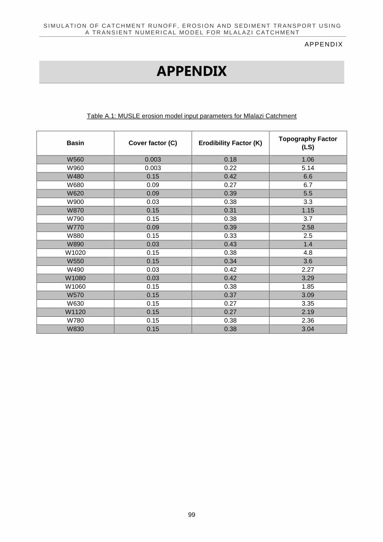
S I MU L A TI O N O F C A TC H ME N T R U N O F F , E R OS I O N A N D S E DI ME N T TR A N S P O R T U S I N G A TR A N S I E N T N U ME R I C A L MO D E L F O R ML A L A Z I C A TC H ME N T
APPENDIX
99
APPENDIX
Table A.1: MUSLE erosion model input parameters for Mlalazi Catchment
Basin Cover factor (C) Erodibility Factor (K) Topography Factor
(LS)
W560 0.003 0.18 1.06
W960 0.003 0.22 5.14
W480 0.15 0.42 6.6
W680 0.09 0.27 6.7
W620 0.09 0.39 5.5
W900 0.03 0.38 3.3
W870 0.15 0.31 1.15
W790 0.15 0.38 3.7
W770 0.09 0.39 2.58
W880 0.15 0.33 2.5
W890 0.03 0.43 1.4
W1020 0.15 0.38 4.8
W550 0.15 0.34 3.6
W490 0.03 0.42 2.27
W1080 0.03 0.42 3.29
W1060 0.15 0.38 1.85
W570 0.15 0.37 3.09
W630 0.15 0.27 3.35
W1120 0.15 0.27 2.19
W780 0.15 0.38 2.36
W830 0.15 0.38 3.04

S I MU L A TI O N O F C A TC H ME N T R U N O F F , E R OS I O N A N D S E DI ME N T TR A N S P O R T U S I N G A TR A N S I E N T N U ME R I C A L MO D E L F O R ML A L A Z I C A TC H ME N T
APPENDIX
100
ANNEXURE A: CANDIDATE’S ORIGINALITY DECLARATION (RESEARCH PAPERS, MINI-
DISSERTATIONS, DISSERTATIONS AND THESES)
ORIGINALITY DECLARATION
Full Names and Surname Khathutshelo Joshua Rasifudi
Student Number 201454749
Title of dissertation/thesis Simulation of catchment runoff, erosion and sediment transport using a
transient numerical model for Mlalazi Catchment
I acknowledge that I have read and understood the University's policies and rules applicable to
postgraduate research, and I certify that I have, to the best of my knowledge and belief,
complied with their requirements.
In particular, I confirm that I had obtained an ethical clearance certificate for my research
(Certificate Number UZREC 171110-030 PGM 2018/592) and that I have complied with the
conditions set out in that certificate.
I further certify that this dissertation is original, and that the material has not been published
elsewhere, or submitted, either in whole or in part, for a degree at this or any other university.
I declare that this dissertation is, save for the supervisory guidance received, the product of my
own work and effort. I have, to the best of my knowledge and belief, complied with the
University’s Plagiarism Policy and acknowledged all sources of information in line with normal
academic conventions.
I have subjected the document to the University’s text-matching and/or similarity-checking
procedures.
Candidate’s signature
Date
25/10/2018

S I MU L A TI O N O F C A TC H ME N T R U N O F F , E R OS I O N A N D S E DI ME N T TR A N S P O R T U S I N G A TR A N S I E N T N U ME R I C A L MO D E L F O R ML A L A Z I C A TC H ME N T
APPENDIX
101
ANNEXURE B: UNIVERSITY’S RESEARCH ETHICS DECLARATION AND CERTIFICATE

S I MU L A TI O N O F C A TC H ME N T R U N O F F , E R OS I O N A N D S E DI ME N T TR A N S P O R T U S I N G A TR A N S I E N T N U ME R I C A L MO D E L F O R ML A L A Z I C A TC H ME N T
APPENDIX
102