Arun K. Tangirala · 2017-08-04 · Wiener-Khinchin Theorem Recall that the DTFT of a sequence exists only if it is absolutely convergent. Thus, the p.s.d. of a signal is deﬁned

Spectral Representations of Random Processes References

CH5350: Applied Time-Series Analysis

Arun K. Tangirala

Department of Chemical Engineering, IIT Madras

Spectral Representations of Random Signals

Arun K. Tangirala (IIT Madras) Applied Time-Series Analysis 1


Opening remarks

We have learnt, until this point, how to represent deterministic signals (and systems) in

the frequency-domain using Fourier series / transforms.

I Signal decomposition results in also energy / power decomposition (as the case

maybe) by virtue of Parseval’s relations.

I Signal decomposition is primarily useful in filtering and signal estimation, whereas

power / energy decomposition is useful in detection of periodic components /

frequency content of signals.

I Fourier analysis, as we have seen, is the key to characterizing the frequency response

of LTI systems and analyzing their “filtering” nature,



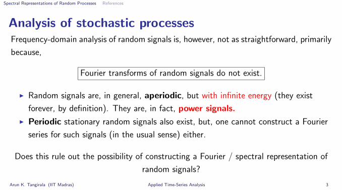
Analysis of stochastic processesFrequency-domain analysis of random signals is, however, not as straightforward, primarily

because,

Fourier transforms of random signals do not exist.

I Random signals are, in general, aperiodic, but with infinite energy (they exist

forever, by definition). They are, in fact, power signals.

I Periodic stationary random signals also exist, but, one cannot construct a Fourier

series for such signals (in the usual sense) either.

Does this rule out the possibility of constructing a Fourier / spectral representation of

random signals?



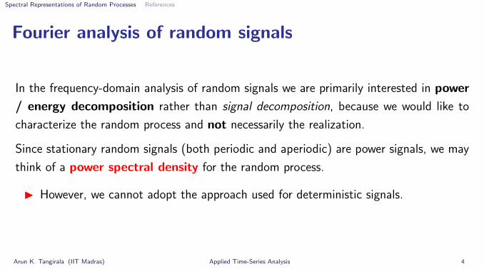
Fourier analysis of random signals

In the frequency-domain analysis of random signals we are primarily interested in power

/ energy decomposition rather than signal decomposition, because we would like to

characterize the random process and not necessarily the realization.

Since stationary random signals (both periodic and aperiodic) are power signals, we may

think of a power spectral density for the random process.

I However, we cannot adopt the approach used for deterministic signals.



Spectral analysis of random signals

A rigorous way of defining power spectral density (p.s.d.) of a random signal is through

Wiener’s generalized harmonic analysis (GHA). Roughly stated, the GHA is an

extension of Fourier transforms / series to handle random signals, wherein the Fourier

transforms / coe�cients of expansion are random variables.

An alternative route takes a semi-formal approach to arrive at the same expression for

p.s.d. as through Weiner’s GHA. The most widely used route is, however, through the

Wiener-Khinchin relation.



Three di↵erent approaches to p.s.d.

1. Semi-formal approach: Construct the spectral density as the ensemble average of the

empirical spectral density of a finite-length realization in the limit as N ! 1.

2. Wiener-Khinchin relation: One of the most fundamental results in spectral analysis of

stochastic processes, it allows us to compute the spectral density as the Fourier

transform of the ACVF. This is perhaps the most widely used approach.

3. Wiener’s GHA: A generalization of the Fourier analysis to the class of signals which are

neither periodic nor finite-energy, aperiodic signals (e.g., cosp2k). It is theoretically

sound, but also involves the use of advanced mathematical concepts, e.g., stochastic

integrals.

Focus: First two approaches and the conditions for the existence of a spectral density.Arun K. Tangirala (IIT Madras) Applied Time-Series Analysis 6


Semi-formal approach

Consider a length-N sample record of a random signal. Compute the periodogram, i.e.,

the empirical p.s.d., of the finite-length realization

�(i,N)vv (!n) =

|VN(!n)|2

2⇡N=

1

2⇡N

��

N�1X

k=0

v(i)[k]e�j!nk

��

2

where VN(!n) is the N -point DFT of the finite length realization.



Semi-formal approach

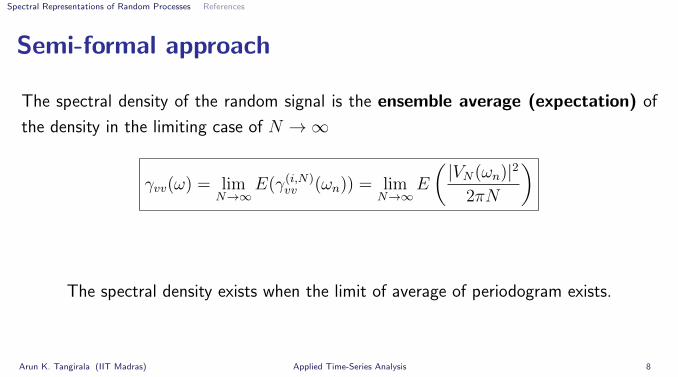
The spectral density of the random signal is the ensemble average (expectation) of

the density in the limiting case of N ! 1

�vv(!) = lim

N!1E(�(i,N)

vv (!n)) = lim

N!1E

✓|VN(!n)|2

2⇡N

◆

The spectral density exists when the limit of average of periodogram exists.



When does the empirical definition exist?

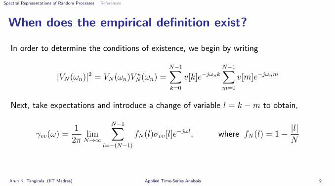
In order to determine the conditions of existence, we begin by writing

|VN(!n)|2 = VN(!n)V?N(!n) =

N�1X

k=0

v[k]e�j!nkN�1X

m=0

v[m]e�j!nm

Next, take expectations and introduce a change of variable l = k �m to obtain,

�vv(!) =1

2⇡lim

N!1

N�1X

l=�(N�1)

fN(l)�vv[l]e�j!l, where fN(l) = 1� |l|

N



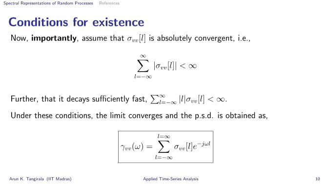
Conditions for existenceNow, importantly, assume that �vv[l] is absolutely convergent, i.e.,

1X

l=�1

|�vv[l]| < 1

Further, that it decays su�ciently fast,P1

l=�1 |l|�vv[l] < 1.

Under these conditions, the limit converges and the p.s.d. is obtained as,

�vv(!) =

l=1X

l=�1

�vv[l]e�j!l



Wiener-Khinchin Theorem

Recall that the DTFT of a sequence exists only if it is absolutely convergent. Thus, the

p.s.d. of a signal is defined only if its ACVF is absolutely convergent.

This leads us to the familiar Wiener-Khinchin theorem or the spectral

representation theorem.



Spectral Representation / Wiener-Khinchin TheoremW-K Theorem (Shumway and Sto↵er, 2006)Any stationary process with ACVF �vv[l] satisfying

1X

l=�1

|�vv[l]| < 1 (absolutely summable)

has the spectral representation

�vv[l] =

Z ⇡

�⇡

�vv(!)ej!l d!, where �vv(!) =

1

2⇡

1X

l=�1

�vv[l]e�j!l �⇡ ! < ⇡

�vv(!) is known as the spectral density.



W-K Theorem: Remarks

I It is one of the milestone results in the analysis of linear random processes.

I Recall that a similar version also exists for aperiodic, finite-energy, deterministic

signals. The p.s.d. is replaced by e.s.d. (energy spectral density). Thus, it provides

a unified definition for both deterministic and stochastic signals.

I It establishes a direct connection between the second-order statistical properties in

time to second-order properties in frequency domain.

I The inverse result o↵ers an alternative way of computing the ACVF of a signal.

A more general statement of the theorem unifies both classes of random signals, the ones with absolutely

convergent ACVFs and the ones with periodic ACVFs (harmonic processes).



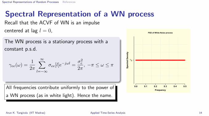
Spectral Representation of a WN processRecall that the ACVF of WN is an impulse

centered at lag l = 0,

The WN process is a stationary process with a

constant p.s.d.

�ee(!) =1

2⇡

1X

l=�1�ee[l]e

�j!l=

�2e

2⇡, �⇡ ! ⇡

All frequencies contribute uniformly to the power of

a WN process (as in white light). Hence the name.

PSD of White-Noise process

Frequency

Sp

ec

tra

l D

en

sit

y

!2

0.0 0.1 0.2 0.3 0.4 0.5



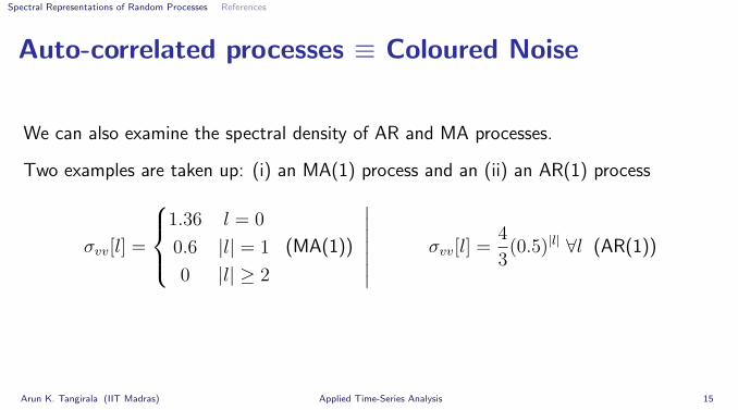
Auto-correlated processes ⌘ Coloured Noise

We can also examine the spectral density of AR and MA processes.

Two examples are taken up: (i) an MA(1) process and an (ii) an AR(1) process

�vv[l] =

8><

>:

1.36 l = 0

0.6 |l| = 1

0 |l| � 2

(MA(1))

��vv[l] =

4

3

(0.5)|l| 8l (AR(1))



PSD of MA(1) and AR(1) processes

0.0 0.1 0.2 0.3 0.4 0.5

0.5

1.0

1.5

2.0

2.5

PSD of an MA(1) process: x[k] = e[k] + 0.6e[k-1]

Frequency

Sp

ec

tra

l D

en

sit

y

The spectral density is a func-

tion of the frequency unlike

the “white” noise. Correlated

processes therefore acquire the

name coloured noise.

0.0 0.1 0.2 0.3 0.4 0.5

0.5

1.0

1.5

2.0

2.5

3.0

3.5

4.0

PSD of an AR(1) process: x[k] = 0.5x[k-1] + e[k]

Frequency

Sp

ec

tra

l D

en

sit

y



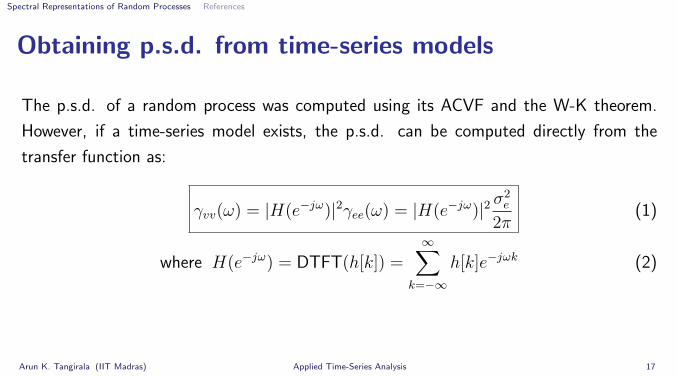
Obtaining p.s.d. from time-series models

The p.s.d. of a random process was computed using its ACVF and the W-K theorem.

However, if a time-series model exists, the p.s.d. can be computed directly from the

transfer function as:

�vv(!) = |H(e�j!)|2�ee(!) = |H(e�j!

)|2 �2e

2⇡(1)

where H(e�j!) = DTFT(h[k]) =

1X

k=�1

h[k]e�j!k (2)



PSD from Model

Derivation: Start with the general definition of a linear random process

v[k] =

1X

m=�1h[m]e[k �m] =) �vv[l] =

1X

m=�1h[m]h[l �m]�2

ee

Taking (discrete-time) Fourier Transform on both sides yields the main result.

The p.s.d. of a linear random process is / the squared magnitude of its FRF


Documents

Arun K. Tangirala · 2017-08-04 · Wiener-Khinchin Theorem Recall that the DTFT of a sequence exists only if it is absolutely convergent. Thus, the p.s.d. of a signal is deﬁned