Arun K. Tangirala...Probability & Statistics - Review 2 Multivariate analysis In the analysis of several statistical events and random signals we will be required to analyze two or

Probability & Statistics - Review 2

CH5350: Applied Time-Series Analysis

Arun K. Tangirala

Department of Chemical Engineering, IIT Madras

Probability & Statistics: Bivariate / Multivariate case

Arun K. Tangirala Applied Time-Series Analysis 1


Multivariate analysis

In the analysis of several statistical events and random signals we will be required to

analyze two or more variables simultaneously. Of particular interest would be to examine

the presence of linear dependencies, develop linear models and predict one RV using

another set of random variables.

We shall primarily study bivariate analysis, i.e., analysis of a pair of random variables.



Bivariate analysis and joint p.d.f.

Where bivariate analysis is concerned, we start to think of joint probability density

functions, i.e., the probability of two RVs taking on values within a rectangular cell in

the 2-D real space.

Examples:

I Height and weight of an individual

I Temperature and pressure of a gas



Joint density

Consider two continuous-valued RVs X and Y . The probability that these variables take

on values in a rectangular cell is given by the joint density

Pr(x1 x x2, y1 y y2) =

Zy2

y1

Zx2

x1

f(x, y) dx dy



Joint Gaussian density

The joint Gaussian density function of two RVs is given by

f(x, y) =

1

2⇡|⌃Z|1/2exp

✓�1

2

(Z� µZ

)

T

⌃

�1Z

(Z� µZ)

◆(1)

where

Z =

"X

Y

#⌃Z =

"�

2X

�

XY

�

XY

�

2Y

#(2)

The quantity �XY

is known as the covariance and ⌃Z the variance-covariance matrix.



Marginal and conditional p.d.f.s

Associated with this joint probability (density function), we can ask two questions:

1. What is the probability Pr(x1 X x2) regardless of the outcome of Y and vice

versa? (marginal density)

2. What is the probability Pr(x1 X x2) given Y has occurred and taken on a

value Y = y? (conditional density)

I Strictly speaking, one cannot talk of Y taking on an exact value, but only of

values within an infinitesimal neighbourhood of y.



Marginal density

The marginal density is arrived at by walking across the outcome space of the “free”

variable and adding up the probabilities of the free variable within infinitesimal intervals.

The marginal density of a RV X with respect to another RV Y is given by

f

X

(x) =

Z 1

�1f(x, y) dy (3)

Likewise,

f

Y

(y) =

Z 1

�1f(x, y) dx (4)



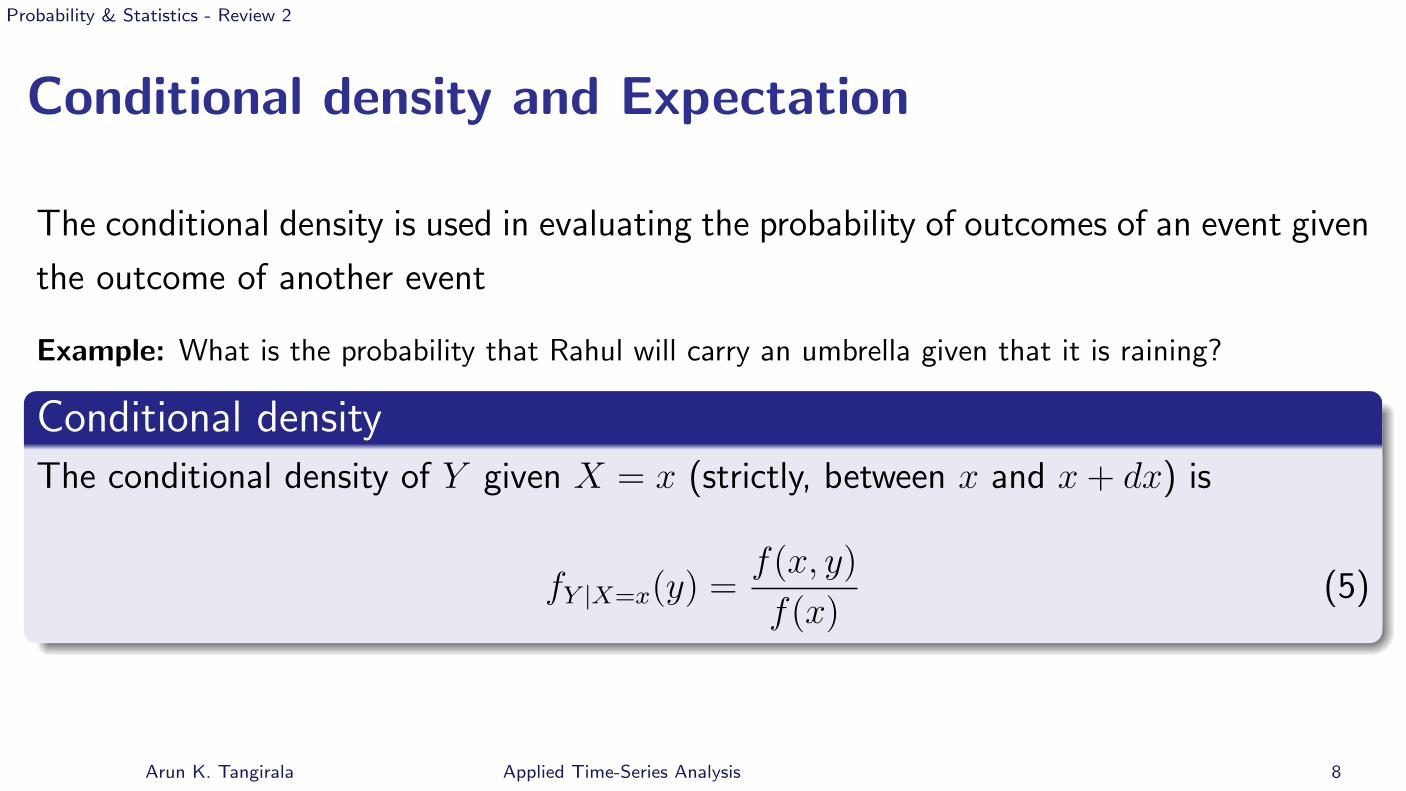
Conditional density and Expectation

The conditional density is used in evaluating the probability of outcomes of an event given

the outcome of another event

Example: What is the probability that Rahul will carry an umbrella given that it is raining?

Conditional densityThe conditional density of Y given X = x (strictly, between x and x+ dx) is

f

Y |X=x

(y) =

f(x, y)

f(x)

(5)



Conditional Expectation

In several situations we are interested in “predicting” the outcome of one phenomenon

given the outcome of another phenomenon.

Conditional expectationThe conditional expectation of Y given X = x is

E(Y |X = x) =

Z 1

�1yf

Y |X=x

(y) dy (6)



Conditional expectation and prediction

The conditional expectation of Y given X = x is a function of x, i.e.,

E(Y |X = x) = �(x)

The conditional expectation is the best predictor of Y given X among all the pre-

dictors that minimize the mean square prediction error

Note: We shall prove this result later in the lecture on prediction theory.



Iterative expectation

A useful result involving conditional expectations is that of iterative expectation.

Iterative Expectation

E

X

(E

Y

(Y |X)) = E(Y ) ;E

Y

(E

X

(X|Y )) = E(X)

In evaluating the inner expectation, the quantity that is fixed is treated as deterministic.

The outer expectation essentially averages the inner one over the outcome space of the

fixed inner variable.



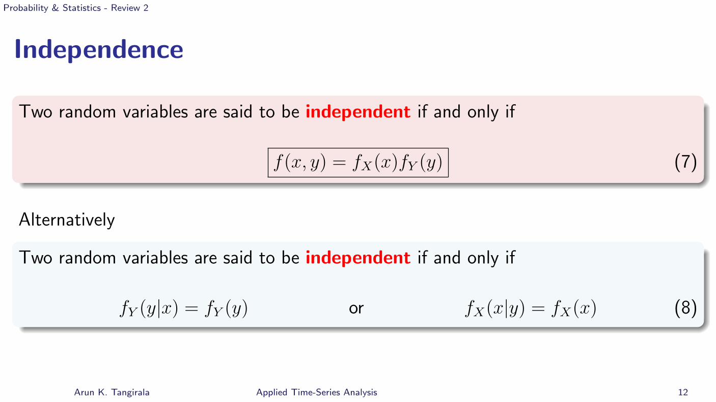
Independence

Two random variables are said to be independent if and only if

f(x, y) = f

X

(x)f

Y

(y) (7)

Alternatively

Two random variables are said to be independent if and only if

f

Y

(y|x) = f

Y

(y) or f

X

(x|y) = f

X

(x) (8)



CovarianceOne of the most interesting questions in bivariate analysis and prediction theory is if the

outcomes of two random variables influence each other, i.e., whether they co-vary.

The statistic that measures the co-variance between two RVs is given by

�

XY

= E((X � µ

X

)(Y � µ

Y

)) =

Z +1

�1

Z +1

�1(x� µ

X

)(y � µ

Y

)f(x, y) dx dy (9)

Covariance, second-order property of the joint p.d.f., can further be shown as

�

XY

= E((X � µ

X

)(Y � µ

Y

)) = E(XY )� E(X)E(Y ) (10)

I Clearly, if Y = X, we obtain variance of X, the spread of outcomes of X

I Therefore, covariance is a measure of joint spread of X and Y



Covariance for vector quantities

The covariance and variance of a pair of random variables X1 and X2 are collected in a

single matrix, known as the variance-covariance matrix

⌃

X

=

"�

2X1

�

X1X2

�

X2X1 �

2X2

#



Vector caseIn the general case, for a vector of random variables,

X =

hX1 X2 · · · X

N

iT

the matrix is given by,

⌃X = E((X� µX)(X� µX)T

)

=

2

66664

�

2X1

�

X1X2 · · · �

X1XN

�

X2X1 �

2X2

· · · �

X2XN

... · · · · · · ...

�

XNX1 �

XNX2 · · · �

2XN

3

77775



Properties of the covariance matrix

The covariance (matrix) possesses certain properties which have far-reaching implications

in analysis of random processes.

I Covariance is a second-order property of the joint probability density function

I It is a symmetric measure: �XY

= �

Y X

, i.e., it is not a directional measure.

Consequently it cannot be used to sense causality (cause-e↵ect relation).

I The covariance matrix ⌃X is a symmetric, positive semi-definite matrix

=) �

i

(⌃X) � 0 8 i

I Number of zero eigenvalues of ⌃Z = Number of linear relationships in Z

(cornerstone for principal component analysis and multivariate regression)



Properties of the covariance matrix

I Linear transformation of the random variables Z = AX results in

⌃Z = E((Z� µZ)(Z� µZ)T

) = A⌃XAT (11)

I Most importantly, covariance is only a measure of linear relationship between

two RVs, i.e.,

When �

XY

= �

Y X

= 0, there is no linear relationship between X and Y



CorrelationTwo issues are encountered with the use of covariance in practice:

i. Covariance is sensitive to the choice of units for the random variables under investigation.

Stated otherwise, it is sensitive to scaling.

ii. It is not a bounded measure, meaning it is not possible to the infer the degree of the

strength of the linear relationship from the value of �XY

To overcome these issues, a normalized version of covariance known as correlation is

introduced:

⇢

XY

=

�

XY

�

X

�

Y

(12)

I The correlation defined above is also known as Pearson’s correlation

I Other forms of correlations exist, namely, reflection correlation coe�cient, Spearman”s rank

correlation coe�cient, Kendall’s tau rank correlation coe�cient



Properties of correlationCorrelation enjoys all the properties that covariance satisfies,i.e., symmetricity and ability

to detect linear relationships, etc.

Importantly, correlation is a bounded measure, i.e., |⇢XY

| 1

BoundednessFor all bivariate distributions with finite second order moments,

|⇢XY

| 1 (13)

with equality if, with probability 1, there is a linear relationship between X and Y .

The result can be proved using Chebyshev’s inequalityArun K. Tangirala Applied Time-Series Analysis 19


Unity correlation

Correlation measures linear dependence. Specifically,

i. ⇢

XY

= 0 () X and Y have no linear relationship (non-linear relationship cannot

be detected)

ii. |⇢XY

| = 1 () Y = ↵X + � (Y and X are linearly related with or without an

intercept)



Unity correlation . . . contd.

Assume Y = ↵X. Then, µY

= ↵µ

X

; �

2Y

= ↵

2�

2X

⇢

XY

=

E(XY )� E(X)E(Y )

�

X

�

Y

=

↵(E(X)

2 � E(X)

2)

|↵|�2X

=

↵

|↵|= ±1



Uncorrelated variables

Uncorrelated variablesTwo random variables are said to be uncorrelated if �

XY

= 0 =) ⇢

XY

= 0.

Alternatively, since �

XY

= E(XY )� E(X)E(Y ), the condition also implies

E(XY ) = E(X)E(Y ) (14)

I Uncorrelatedness () NO linear relationship between X and Y .

I Determining the absence of non-linear dependencies requires the test of

independence.



Independence vs. Uncorrelated variables

Independence =) Uncorrelated condition but NOT vice versa.

Thus independence is a stronger condition.

If the variables X and Y have a bivariate Gaussian distribution,

Independence () Uncorrelated condition.

Therefore, in all such cases, independence and lack of correlation are equivalent.



Conditional expectation and Covariance

The conditional expectation essentially gives the expectation of Y given X = x. In-

tuitively, if there is a linear relationship between Y and X, the conditional expectation

should be expected to be di↵erent from the unconditional expectation. Theoretically,

Two variables are uncorrelated if E(Y |X) = E(Y )

The result can be proved using iterative expectation. See text (p. 168) for details.

Remark: The result is similar to that for independence: f(y|x) = f(y) (conditional = marginal)



Correlation values less than unity - implications

The magnitude of correlation in practice is never likely to touch unity since no process

is truly linear. Therefore, it is useful to quantify the e↵ects of factors that contribute to

the fall of correlation (in magnitude) below unity:

I Non-linearities and / or modelling errors

I Measurement noise and / or e↵ects of unmeasured disturbances



A common scenario: linear relation plus noise, etc.

Assume a r.v. Y is made up of a linear e↵ect ↵X and an additional element ✏, Y = ↵X+✏

s.t. (i) µ✏

= 0 =) µ

Y

= ↵µ

X

and (ii) ✏ and X are uncorrelated, i.e., there is nothing in

✏ that can be explained by a linear function of X (reasonable assumption).

Then, it can be shown that

⇢

Y X

= ± 1s

1 +

�

2✏

↵

2�

2X

±1



Signal-to-Noise Ratio (SNR) and Non-linearities

I When ✏ represents merely the measurement error in Y , the ratio↵

2�

2X

�

2✏

is known as

the signal-to-noise ratio (SNR). Thus, even when the true relationship is linear,

SNR can cause a significant dip in the correlation. In fact, as SNR ! 0, ⇢Y X

! 0

I When ✏ represents the non-linearities and other factors that are uncorrelated with

X, the ratio↵

2�

2X

�

2✏

represents the variance-explained to prediction-error ratio. Once

again when �

2✏

� ↵

2�

2X

, ⇢Y X

⇡ 0

In practice, ✏ contains both unexplained non-linear e↵ects and noise. It is hard to distinguish

the individual contributions, but the net e↵ect is a drop in the correlation.



Connections b/w Correlation and Linear regression

Correlation between two RVs is naturally related to linear regression of one variable on

the other.

Given two (zero-mean) RVs X and Y , consider the linear predictor of Y in terms of X

ˆ

Y = bX (15)

The optimal estimate b that minimizes E("

2) = E(Y � ˆ

Y )

2 is

b

?

=

�

XY

�

2X

= ⇢

XY

�

Y

�

X

(16)



Correlation and regression . . . contd.Similarly, the optimal coe�cient of the reverse predictor, ˆ

X =

˜

bY , is

˜

b

?

=

�

XY

�

2Y

= ⇢

XY

�

X

�

Y

(17)

We make an interesting observation,

⇢

2XY

= b

?

˜

b

? (18)

Correlation captures linear e↵ects in both directions.



Correlation and regression . . . contd.Further, (for the X ! Y model)

cov(", X) = cov(Y � b

?

X,X) = 0 (residual ? regressor) (19)

�

2"

= �

2Y

� b

?

2�

2X

= �

2Y

(1� ⇢

2XY

) (20)

so that the standard theoretical measures of fit for both (directional) models are

R

2X!Y

= 1� �

2"

�

2Y

= ⇢

2XY

= R

2Y!X

(21)

Zero correlation implies no linear fit in either direction.



Remarks, limitations, . . .

I Correlation is only a mathematical / statistical measure. It does not take

into account any physics of the process that relates X to Y .

I High values of correlation only means that a linear model can be fit between X and

Y . It does not mean that in reality there exists a linear process that relates X to Y

I Correlation is symmetric, i.e., ⇢XY

= ⇢

Y X

. Therefore, it is not a cause-e↵ect

measure, meaning it cannot detect direction of relationships

I Correlation is primarily used to determine if a linear model can explain the

relationship:



Remarks, limitations, . . . . . . contd.

I High values of estimated correlation may imply linear relationship over the

experimental conditions, but a non-linear relationship over a wider range.

I Absence of correlation only implies that no linear model can be fit. Even if

the true relationship is linear, noise can be high, thus limiting the ability of

correlation to detect linearity

I Correlation measures only linear dependencies. Zero correlation means

E(XY ) = E(X)E(Y ). In contrast, independence implies f(x, y) = f(x)f(y)

Despite its limitations, correlation and its variants remain one of the most widely used

measures in data analysis



Confounding

When two variables X and Y are correlated, a question that begs attention is:

Q: Are X and Y connected to each other directly or indirectly?

Conditional measures provide the answer.



Conditional correlation

Z

X Y

direct link

confounding variable Z

X.Z Y.Z

conditioning

I If the conditional correlation vanishes, then the connection is purely indirect,

else there exists a direct relation

Correlation measures total (linear) connectivity, whereas conditional or partial version

measures “direct” association.



Partial covariance

The conditional or partial covariance is defined as

�

XY.Z

= cov(✏X.Z

, ✏

Y.Z

) where ✏

X.Z

= X � ˆ

X

?

(Z), ✏

Y.Z

= Y � ˆ

Y

?

(Z)

where ˆ

X

?

(Z) and ˆ

Y

?

(Z) are the optimal predictions of X and Y using Z.



Partial correlation

Partial correlation (PC)

⇢

XY.Z

=

�

XY.Z

�

✏X.Z�✏Y.Z

=

⇢

XY

� ⇢

XZ

⇢

ZYp(1� ⇢

2XZ

)

p(1� ⇢

2ZY

)

(22)

I Can be extended to more-than-three variables case as well.

I Partial correlation ⌘ Analysis in the inverse domain.



Partial correlation: Example

Consider two random variables X = 2Z + 3W and Y = Z + V where V , W and Z are

zero-mean RVs. Further, it is known that W and V are uncorrelated with Z as well as

among themselves, i.e., �VW

= 0.

Evaluating the covariance between X and Y yields

�

Y X

= E((2Z + 3W )(Z + V )) = 2E(Z

2) = 2�

2Z

6= 0

although X and Y are not “directly” correlated.



Partial correlation: Example

Now,

⇢

Y X

=

�

2Z

(�

2Z

+ �

2Y

)(4�

2Z

+ �

2W

)

; ⇢

Y Z

=

1s

1 +

�

2V

�

2Z

; ⇢

XZ

=

1s

1 +

�

2V

4�

2Z

;

Next, applying (22), it is easy to see that

⇢

Y X.Z

= 0



Partial correlation by inversion (from covariance)

Partial correlation coe�cients can also be computed from the inverse of covariance

matrix as follows.

Assume we have M RVs X1, X2, · · · , XM

. Let X =

hX1 X2 · · · X

M

iT

.

1. Construct the covariance matrix ⌃X.

2. Determine the inverse of covariance matrix, SX = ⌃

�1X .

3. The partial correlation between X

i

and X

j

conditioned on all X\{Xi

, X

j

} is then:

⇢

XiXj .X\{Xi,Xj} = � s

ijps

ii

ps

jj

(23)



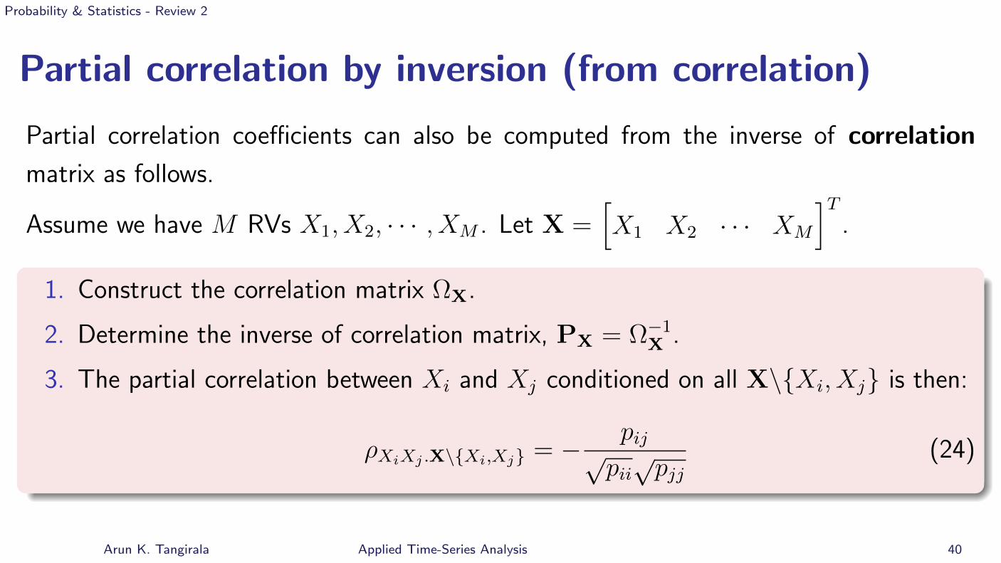
Partial correlation by inversion (from correlation)

Partial correlation coe�cients can also be computed from the inverse of correlation

matrix as follows.

Assume we have M RVs X1, X2, · · · , XM

. Let X =

hX1 X2 · · · X

M

iT

.

1. Construct the correlation matrix ⌦X.

2. Determine the inverse of correlation matrix, PX = ⌦

�1X .

3. The partial correlation between X

i

and X

j

conditioned on all X\{Xi

, X

j

} is then:

⇢

XiXj .X\{Xi,Xj} = � p

ijpp

ii

pp

jj

(24)



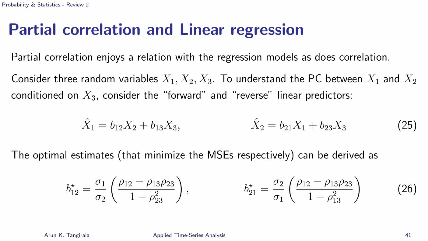
Partial correlation and Linear regression

Partial correlation enjoys a relation with the regression models as does correlation.

Consider three random variables X1, X2, X3. To understand the PC between X1 and X2

conditioned on X3, consider the “forward” and “reverse” linear predictors:

ˆ

X1 = b12X2 + b13X3,ˆ

X2 = b21X1 + b23X3 (25)

The optimal estimates (that minimize the MSEs respectively) can be derived as

b

?

12 =�1

�2

✓⇢12 � ⇢13⇢23

1� ⇢

223

◆, b

?

21 =�2

�1

✓⇢12 � ⇢13⇢23

1� ⇢

213

◆(26)



PC and linear regression

We have an interesting result:

The squared-PC between X1 and X2 is the product of optimal coe�cients

⇢

212.3 = b

?

12b?

21 (27)

I Partial correlation captures “direct” dependence in both directions.

I As with correlation, it is also, therefore, an symmetric measure.



Uses of partial correlation

I In time-series analysis, partial correlations are used in devising what are known as

partial auto-correlation functions, which are used in determining the order of

auto-regressive models

I The partial cross-correlation function and its frequency-domain counterpart, known

as partial coherency function, find good use in time-delay estimation

I In model-based control applications, partial correlations are used in quantifying the

impact of model-plant mismatch in model-predictive control applications.



Commands in R

Commands Utility

mean,var,sd sample mean, variance and standard deviation

colMeans,rowMeans means of columns and rows

median,mad sample median and median absolute deviation

cov,corr,cov2cor covariance, correlation and covariance-to-correlation

lm, summary linear regression and summary of fit



Computing partial correlation in R

Use the ppcor package (due to Seongho Kim)

Ipcor: Computes partial correlation for each pair of variables given others.

Syntax: pcormat <- pcor(X)

where X is a matrix with variables in columns. The default is Pearson correlation,

but it can also compute Kendall and Spearman (partial) correlations. Result is

given in pcormat$estimate



Computing semi-partial correlation in R

Use the ppcor package (due to Seongho Kim)

Ispcor: Computes semi-partial correlation

Syntax: spcormat <- spcor(X)

The semi-partial correlation between X and Y given Z is computed as the

correlation between X and Y.Z, i.e., only Y is conditioned on Z. The matrix of

semi-partial correlations is asymmetric



Sample usage

1 w <� rnorm ( 2 0 0 ) ; v <� rnorm ( 2 0 0 ) ; z <� rnorm ( 2 0 0 ) ; # Genera te w, v and z

2 x <� 2⇤ z + 3⇤w; y = z+ v ; # Genera te x and y

3 cor ( cb ind ( x , y ) ) # Compute c o r r e l a t i o n mat r i x between x and y

4 pcor ( cb ind ( x , y , z ) ) ) $ e s t ima t e # Compute p a r t i a l c o r r e l a t i o n mat r i x


Documents

Arun K. Tangirala...Probability & Statistics - Review 2 Multivariate analysis In the analysis of several statistical events and random signals we will be required to analyze two or