arX

iv:h

ep-p

h/98

0335

1v1

13

Mar

199

8

ANL-HEP-PR-98-08

JLAB-THY-98-08

hep-ph/9803351

March 13, 1998

x-Dependent Polarized Parton Distributions

Lionel E. Gordona,b,c Mehrdad Goshtasbpourd,e and Gordon P. Ramseyf,c

a) Thomas Jefferson National Lab, Newport News, VA 23606

b) Hampton University, Hampton, VA 23668

c) Argonne National Lab, Argonne, IL 60439 ∗

d) Shahid Beheshti University, Tehran, Iran

e) Center For Theoretical Physics and Mathematics, AEOI, Tehran, Iran

f) Loyola University, Chicago, IL 60626

Abstract

Using QCD motivated and phenomenological considerations, we construct x de-

pendent polarized parton distributions, which evolve under GLAP evolution, satisfy

DIS data and are within positivity constraints. Each flavor is done separately and the

overall set can be used to predict polarization asymmetries for various processes. We

perform our NLO analysis strictly in x space, avoiding difficulties in moment inversion.

Small-x results and other physical considerations are discussed.

PACS: 13.60.Hb, 13.88.+e, 14.20.Dh

∗Work supported in part by the U.S. Department of Energy, Division of High Energy Physics, ContractW-31-109-ENG-38.

I. Introduction

In light of recent polarized deep-inelastic-scattering data, there has been considerable

interest in generating x-dependent parton distributions for the spin-dependent case. Physics

results have been extracted from the integrated structure functions [1-3]. The results indicate

that there is still considerable uncertainty in the fraction of spin carried by the gluons and sea

quarks. Each of the analyses rely on certain assumptions to model the polarized distributions.

One important way to test these assumptions is to generate the x-dependent distributions

and predict spin observables, such as the structure functions, g1, for the proton, neutron

and deuteron, hard scattering cross sections for polarized hadronic collisions and hadronic

production of pions, Kaons and heavy quark flavors. The structure function measurements

of g1 have been made, but the distributions at small-x are still quite uncertain.

There are various sets of x-dependent polarized distributions which extract the un-

known parameters from assumptions about the data [3-9]. Most of these are consistent with

the x-dependent data, but do not adequately address the physical questions of compatibility

with the integrated data (and hence the spin fractions of the partons) and the positivity

constraints for each flavor. The usual approach is to fit the polarized data directly with a

given parametrization, and then check the integrals for agreement with the extracted frac-

tions of spin carried by the quark flavors (or set normalizations to fit the spin fractions).

Often, either the valence is not considered separately or the flavor dependence of the sea is

not considered.

Our approach is to establish a reasonable set of flavor-dependent distributions at an

initial Q20, motivated by physical constraints and data, then evolve to arbitrary Q2 for use

in predicting polarized observables. This approach is unique in many aspects. The distri-

butions begin with information from the integrated distributions and impose normalization

and positivity constraints (all flavors, valence and sea) to ensure that all of the spin infor-

mation extracted from data is explicitly contained in the x-dependent results. We generate

polarized parton distributions from the unpolarized distributions and well defined suitable

assumptions, derived from the most recent polarized deep-inelastic-scattering (PDIS) data

sets available [10-15].

For the polarized sea, we assume a broken SU(3) model, to account for mass effects in

1

polarizing the sea. Our models separate out all flavors in the valence and sea for a complete

analysis of the flavor dependence of the spin fractions in hadrons. We include charm via

the evolution equations (Nf), at the appropriate Q2 of charm production, to avoid any

non-empirical assumptions about its size. The entire LO and NLO analysis is done in x-

space to avoid the potential pitfalls of losing kinematical information in the inversion of

moments. Physically, the small-x behavior is of the Regge type, consistent with data and

other theoretical approaches [2]. The large-x behavior is compatible with the appropriate

counting rules [16].

We consider three distinct models for the polarized gluons, which have a moderately

wide range. Our choice effectively includes two separate factorization schemes: Gauge In-

variant (GI) and Chiral Invariant (CI). These are all physically motivated models, whose

overall size not large. The final parametrizations are easy to use, both in form and format.

They are also in excellent agreement with the most recent data.

II. Theoretical Background

A. Polarized Quark Distributions

Any distributions that are to be used to predict physical observables must be consistent

with both existing, related data and certain fundamental theoretical assumptions. In the

case of the polarized distributions, the spin information as it applies to hadronic structure

must be implicitly included, and the appropriate kinematic behavior must be explicit, so that

they satisfy the fundamental constraints. This major requirement covers both the theoretical

and experimental considerations which are important. Thus, we wish to construct the x-

dependent polarized valence and sea quark distributions subject to the following physical

constraints:

• the integration over x should reproduce the values extracted from PDIS data, so that

the fraction of spin carried by each constituent is contained implicitly in the flavor-

dependent distributions

• the distributions should reproduce the x-dependent polarized structure functions, gi1,

i=p,n and d at the average Q2 values of the data

• the small-x behavior of g1(x) should fall between a Regge quark-like power of x and a

2

gluon-dominated logarithmic behavior

• the Q2 behavior of the quark distributions should be consistent with the non-singlet

and singlet NLO evolution equations, for the number of flavors appropriate to the Q2

range to be covered

• the positivity constraints are satisfied for all of the flavors.

The first two constraints build in compatibility with both the integrated and the x-

dependent polarized deep-inelastic-scattering (PDIS) data. The third and fourth conditions

satisfy sound theoretical assumptions about both the x and Q2 kinematical dependence of

the distributions. Finally, the last constraint is fundamental to our physical understanding

of polarization.

Valence and Sea Quark Assumptions

We construct the polarized valence distributions from the unpolarized distributions by

imposing a modified SU(6) model [17, 18]:

∆uv(x) ≡ cos θD(x)[uv(x)−2

3dv(x)],

∆dv(x) ≡ cos θD(x)[−1

3dv(x)],

(2.1)

where the spin dilution factor is given by: cos θD ≡ [1 +R0(1− x)2/√x]−1. The R0 term is

chosen to satisfy the Bjorken Sum Rule (BSR), including the appropriate QCD corrections.

In the Q2 region of the present PDIS data, we find that R0 ≈ 2αs

3. We may choose the

unpolarized valence distributions uv and dv as either the MRS [19]:

xuv(x) = 2.43x0.6(1− x)3.69[1− 1.18√x+ 6.18x],

xdv(x) = 0.14x0.24(1− x)4.43[1 + 5.63√x+ 25.5x],

(2.2)

or the CTEQ [20]:

xuv(x) = 1.344x0.501(1− x)3.689[1 + 6.402x0.873],

xdv(x) = 0.640x0.501(1− x)4.247[1 + 2.690x0.333],(2.3)

or equivalent.

3

If we assume a model of the sea obtaining its polarization from gluon Bremsstrahlung,

then the polarized distributions naively would have a form ∆qf = xqf [21, 22]. However, the

polarized deep-inelastic scattering data appear to imply a negatively polarized sea [1]. If the

integrated structure functions are to agree with data, then the normalization defined by ηav ≡〈∆q〉 / 〈xq〉 must be a part of the proportionality between the polarized and unpolarized

distributions. Meanwhile, the positivity constraint, which requires | ∆q |≤ q for all x,

implies a functional form for the function η(x). The basic idea of the Bremsstrahlung

model, coupled with the implications of the data motivate the following form for the flavor

dependent polarized sea distributions:

∆qf (x) ≡ ηf(x) x qf (x), (2.4)

where q(x) is the x-dependent unpolarized distribution for flavor f . The function η(x) is

chosen to satisfy the normalization constraint:

〈∆qf 〉 =∫ 1

0ηf (x) x qf(x) dx ≡ 〈ηxqf 〉 = ηav 〈xqf 〉 , (2.5)

where ηav is extracted from data for each flavor [1]. Physically, η(x) may be interpreted as

a modification of ∆q due to unknown effects of soft physics at low x. This motivates a form

for η(x), which will be discussed later.

Positivity Constraint

For the purposes of this analysis, we are assuming that the sea quarks are effectively

massless, so each quark has a definite helicity state. In essence, this ignores higher twist

transverse spin effects in the entire kinematic range considered. Thus, there is a probabilistic

interpretation of the parton densities, q, and the net parton distribution is given by: q = q ↑+q ↓. The total polarization is given as the difference of probabilities of finding polarized

↑ and ↓ partons in the nucleon: ∆q ≡ q ↑ −q ↓. In a polarized ↑ proton, this probability

for sea quarks should be less than that of the total unpolarized sea distribution, since every

quark is in a given helicity state. This is the positivity constraint; i.e,

| ∆q(x) |≤ q(x). (2.6)

for all x.

This is valid for the leading order (LO) x-dependent distributions which have a clear

probabilistic interpretation, because there is no intrinsic scheme dependence at this level.

4

The results in the next-to-leading-order (NLO) treatment depend only upon the GLAP

evolution, so there is no problem with constraining the sea quarks using positivity at Q20 in

either case. The valence quarks satisfy the positivity constraint by construction. Although

the probabilistic meaning gives rise to the positivity constraint, it is not clear what role

the chiral and gauge invariant schemes have on this interpretation. In our treatment, the

polarized gluon distribution is assumed small at these low Q2 values, so the schemes are

close enough so that positivity is unaffected. This provides a motivation to choose a zero

∆G model - to investigate the gauge invariant factorization.

Evolution

The polarized partons are grouped in a linear combination which is a singlet of flavor

SUf(3) group and a nonsinglet linear combination of that group. The singlet/non-singlet

designations are useful for delineating certain evolution and factorization properties of the

quarks. These combinations can be related to the usual flavor decomposition, including the

valence, sea and gluons. The nonsinglet term ∆qNS is a linear combination of the triplet a3

axial charge and an octet a8 axial charge of the SUf (3) symmetry. The singlet, ∆Σ is related

to the axial charge, a0 and is normally associated with the axial anomaly, which includes a

gluonic contribution. This depends upon the factorization scheme, which will be discussed

shortly.

The non-singlet term is dominated by the valence distribution, under polarized (∆us,

∆ds) symmetry. Its first moment is scale (Q2) independent in LO. The singlet term has

a definite physical interpretation in the gauge invariant scheme, even though it is scale

dependent. Since we are going to assume a small ∆G in all of our models, this interpretation

will be essentially valid, even in the chiral invariant (Adler-Bardeen) scheme, which separates

out the anomaly. Thus, our distributions are constructed within the positivity constraint,

in both cases. In the NLO analysis, the initial distributions are constructed at a low enough

Q20 value to justify the constraints that we have set. We assume that this Q2

0 is still large

enough that higher-twist effects are negligible [23]. The distributions are then evolved in

NLO, completely independent of any further considerations. In the evolution, the separation

of singlet and non-singlet is faithfully maintained. Thus, we can satisfy all of the important

physical constraints.

Our parton distributions are evolved directly in x-space using an iteration technique

5

first suggested in reference [24] and we use the splitting functions recently calculated in

reference [25]. This method differs from the ’brute force’ technique recently used in reference

[26] and requires less computer time than the conventional evolution in n-moment space. In

addition it eliminates the need to invert from n-moment space and the attendant difficulties

in covering the extreme x-values. As a result, this method is inherently more accurate

than evolving the distributions in moment space. Details of the technique can be found in

reference [27].

B. The Role of Polarized Gluons

Factorization

In PDIS, there are two factorization schemes which can be used to represent the po-

larized sea distributions: the gauge-invariant [28] (or MS) and the chiral invariant [29] (or

Adler-Bardeen) schemes [30]. In the chiral-invariant (AB) scheme, the axial gluon anomaly

term, [31] which depends upon the polarized gluon distribution, is separated out from the

chiral invariant polarized quark distributions. Since the measured distributions must be

gauge invariant, the relation between the two scheme dependent distributions is:

∆q(x)GI = ∆q(x)CI −Nfαs

2π∆G(x), (2.7)

where the GI refers to the gauge-invariant scheme and CI to the chiral-invariant scheme.

Thus, the size of ∆G is relevant in the CI scheme. This, in turn, affects the average η

values extracted for each flavor. Thus, ∆G has an indirect bearing on the polarized sea

distributions. [1]

There exists no empirical evidence that the polarized gluon distribution is very large at

the relatively small Q2 values of the data. In fact, even in the NLO evolution, the polarized

gluon distribution does not evolve significantly between Q2 = 1 andQ2 = 10 GeV2, regardless

of which model is chosen. Data from Fermilab [32] indicate that it is likely small at the Q2

values of existing data. In addition, a theoretical model of the polarized glue, based on

counting rules, implies that ∆G ≈ 12[16]. Other theoretical models substantiate this claim,

as well [33, 34]. However, since we do not know the explicit size of the ∆G in this kinematic

region, we perform our analysis using three distinct physical models. The evolution of ∆G

is then done both in LO and NLO to investigate any possible NLO effects.

6

The first set of η(x) functions, quoted in Table I assumes a moderately polarized glue:

∆G(x) = xG(x) = 31.3x0.41(1− x)6.54[1− 4.64√x+ 6.55x], (2.8)

using an unpolarized MRS glue, normalized to 0.50 or

∆G(x) = xG(x) = 1.123x−0.206(1− x)4.673[1 + 4.269x1.508], (2.9)

for the CTEQ gluon distribution, consistent with the analysis in reference 1.

For the second polarized gluon model, we set ∆G = 0 to determine ηav and parametrize

the η(x) accordingly. This is equivalent to the gauge-invariant scheme, since the anomaly

term vanishes. Any analysis which requires a gauge-independent set of flavor dependent

distributions (such as on the lattice) should use this set of polarized distributions at Q20,

evolved to the appropriate Q2 values. The corresponding η(x) functions are listed in Table

II.

The third gluon model is motivated by an instanton-induced polarized gluon distri-

bution, which gives a negatively polarized glue at small-x [35]. This modified distribution

(normalized to ∆G = −0.23) is given by the best fit to the curve in reference [35]:

∆G(x) = 7(1− x)7[1 + 0.474 ln(x)]. (2.10)

This would allow for instanton based non-perturbative effects at small Q2.

Relation between the sea and glue in g1

The valence polarizations are rather well established from the BSR and the polarized

DIS experiments. The valence quarks are dominant at large x and they give their polarization

to the gluons through Bremsstrahlung, which in turn, creates sea polarization via pair-

production. But the sea quarks share the momentum from the gluon which created the

pair, and thus, each constituent is at lower x than the original valence ”parent”. This is

consistent with the polarized sea being dominant at lower x. The PDIS data imply that the

sea is polarized opposite to that of the valence quarks. The relative size of the negative sea

polarization is an indication as to whether gluon polarization is moderately positive (such

as ∆G = xG, implying that polarization of G carries most of the spin of the proton), nil,

or negative. We expect a larger negatively polarized sea for the last two cases as it must

offset the positive anomaly term proportional to gluons in the chiral-invariant scheme and

7

the Jz = 12sum rule in either scheme. If the polarized sea is smaller (less negative) or the

polarized gluon is large, the gp1 curve will exhibit a sharper rise at small x. When future data

are available with smaller error bars, these scenarios can be better defined to yield the correct

sign and size of ∆G. There may be a possibility to argue a positive proportionality of spin

and momentum of the sea if ∆G is very large. A much larger polarized gluon distribution

can imply either a smaller negatively polarized sea or even a slightly positive polarized sea.

However, this would require a prohibitively large polarized glue at these smaller Q2 values.

We argue that this is not likely for the following reasons:

• (1) when the light-cone wavefunctions at small-x are analyzed, they implicate a nega-

tively polarized sea, [36]

• (2) in order for the sea to be entirely positive, ∆G would have to be prohibitively large

to satisfy the data. The orbital angular momentum would have to be correspondingly

large to satisfy the J=1/2 sum rule. This would also disagree with the implications of

the E704 data, [32]

• (3) Our highly successful fits to the x-dependent data not only indicate that ∆G is

likely moderate at Q2=10 GeV2, but that the data at lower Q2 is fit somewhat better

with even smaller ∆G. This is consistent with the evolution of the polarized gluon

distribution. We also show in Section IV that the growth of ∆G presented by ABFR

[4] is not likely, even in NLO. Thus, our present analysis further strengthens the point

of a smaller ∆G at these lower Q2 values,

• (4) most all other independent analyses agree with the negatively polarized sea.

We conclude that a positively polarized sea and a very large ∆G seem unlikely, given

present data.

C. Extrapolation of Data to Small-x

Extrapolation of gi1 (i = p, n, d) to small-x is important experimentally for determi-

nation of the integrated values of these structure functions. Theoretically, the g1 behavior

at small-x is important to understanding the mechanisms which underlie the physics in this

region. There are various models that attempt to explain the contributions to both F2 and

8

g1 at low-x. The data appear to exhibit growth of these quantities, but since the error bars

are somewhat large, most of the predicted types of behavior cannot be ruled out [37].

At large-x, the valence distributions dominate F2 and g1 and these are more well

determined than the sea distributions, which are more prevalent at small-x. Thus, one must

make suitable assumptions about the behavior of the polarized sea at low-x. Experimental

analyses [14, 12] have tended to assume a relatively constant behavior and extrapolate g1

from its value at about x ∼ 10−2 down to x = 0. A model by Donnachie and Landshoff [38]

assumes that the Pomeron couples via vector γµ so that g1 exhibits a logarithmic behavior:

g1 ∼ ln(1/x). Bass and Landshoff [39] analyze a model of a two-gluon Pomeron which

leads to a slightly more divergent behavior at small-x: g1 ∼ [1 + 2 ln(x)]. If negative parity

Pomeron cuts contribute to the spin-dependent cross section, a divergent behavior of g1

results, [40] corresponding to the singular form: g1 ∼ 1/x ln2(x).

We make no presumptions about the forms of the flavor dependent distributions at

small-x, other than their relation to the unpolarized distributions. The parametrization of

ηf(x) in (2.4) will be determined primarily from normalization and positivity constraints.

Once the polarized sea flavors are generated, we can determine resulting the small-x behavior

of g1 and compare it to these theoretical models.

III. Phenomenology

A. Polarized Quark Flavors

In the work of reference 1, the integrated polarized structure functions were compared

to the spin averaged distributions, to establish a comparison between the spin and momentum

carried by each flavor of quark. The results indicate that the relation is flavor dependent,

but the magnitudes of these ratios (ηav in equation 2.5) are of the same order of magnitude.

Although this does not necessarily imply that there is a direct relation between the two, it

does provide a suitable starting point for generating the polarized distributions from known

unpolarized distributions, which satisfy the data on spin-averaged physical processes. This is

the motivation for the form in equation (2.4) for the polarized flavor-dependent distributions.

The integrated data are satisfied by choosing the parameters in η(x) to satisfy equation (2.5)

and the positivity constraints. We also wish to stay consistent with counting rules at large-

9

x [16]. The small-x behavior can be controlled by the functional form that we choose for

η(x). All of these constraints are to be satisfied at some low value of Q2, and the evolution

equations will ensure that positivity and the kinematical behavior stay consistent at all Q2.

A possible form for η(x), which gives flexibility in satisfying the constraints (2.5) and

(2.6) is: η(x) = a+ bxn. We expect the function to be decreasing with x, since the problems

with positivity (for | ηav |> 1) occur at large x. We chose not to modify the (1−x) dependence

in order to keep the counting rule powers in tact (insofar as the unpolarized distributions

do this) for the large-x behavior. We were able to satisfy the positivity constraint at all x

using this form for η(x).

In the following analysis, we assume the unpolarized distributions in the CTEQ form:

q(x) = A0xA1(1−x)A2(1+A3x

A4). Then, using equation (2.4), we generate the corresponding

polarized distributions for each flavor. An analysis with the MRS distributions yields similar

results.

For the CTEQ distributions, we have

xq(x) =1

2

[

0.255x−0.143(1− x)8.041(1 + 6.112x)∓ 0.071x0.501(1− x)8.041]

, (3.1)

where the (−) holds for u and the (+) for the d flavors. The strange sea has the parametriza-

tion:

xs(x) =[

0.064x−0.143(1− x)8.041(1 + 6.112x)]

. (3.2)

Both of these sets account for the u, d asymmetry in the unpolarized sea.

The corresponding integrated polarized distributions can be written in terms of beta

functions, B(m,n), as:

〈∆q〉 = aA0B(A1 + 2, A2 + 1) + aA0A3B(A1 + A4 + 2, A2 + 1)

− bA0B(A1 + n + 2, A2 + 1)− bA0A3B(A1 + A4 + n + 2, A2 + 1)(3.3)

for the CTEQ distributions. The integral 〈xq〉 can be similarly written and thus the re-

striction on a and b, corresponding to the normalization constraint (2.5) is: a = ηav − bλ,

where

λ ≡ B(A1 + n+ 2, A2 + 1) + A3B(A1 + A4 + n + 2, A2 + 1)

B(A1 + 2, A2 + 1) + A3B(A1 + A4 + 2, A2 + 1), (3.4)

10

for the CTEQ unpolarized distributions.

The positivity constraint in terms of a and b is

| ∆q(x) |q(x)

=| ax+ bxn+1 |≤ 1, (3.5)

for all x ∈ [0, 1]. In the following discussion, we will show how η(x) is generated for the

zero polarized gluon case. The procedure is virtually identical to the other two gluon models

where the anomaly term is present.

When we choose a to satisfy the normalization constraint (2.5) and b to satisfy the

positivity constraint (2.6), the x-dependent polarized distribution for each flavor is deter-

mined from (2.4). These conditions are independent of the set of unpolarized distributions

that is used. However, one must be consistent by using the appropriate set of unpolarized

distributions which were used to determine the function η(x). Therefore, we seek the form

η(x) = (ηav − bλ) + bxn, (3.6)

where both b and n are chosen to satisfy the positivity constraint (3.5). This form of η(x)

is motivated by: (1) associating this function with modifications of ∆q by small-x physics

and (2) keeping the (1− x) dependence in tact to be consistent with counting rule behavior

at large x to the extent that the unpolarized distributions have this desired form [16]. We

can then both satisfy positivity (even at large x) and control the small x behavior, where

the sea and glue are most prominent.

Choice of η(x) at small-x

The polarized sea and the gluon distributions are expected to dominate in the small-x

region. If we assume a strongly polarized negative sea, with ηav < −1 then this defines

a range of b values which satisfy the positivity constraint. The behavior of our Ansatz

η(x) = a + bxn for 0 < n < 1 is suited for small-x dependence. When a certain small-x

behavior is desired, a series of n values can be tried for the best fits to data. In fact, when

0.2 < n < 1.0, it is easier to satisfy both constraints with appropriate choices of a and b.

These values of n allow a wider range of a and b values. However, when 0 < n < 0.2, the

range of possible a and b values which satisfy the constraints gets very small and will not be

the same for all experimental yields of ηav. Thus, it makes it impossible to find a uniform

11

fit for η(x) for each flavor. Since η(x) should be only flavor dependent to have any physical

connection, we must choose n so that a and b will be comparable for all experimental results.

Positivity of n is, in principle, not essential. If we choose a small negative n, we enhance

the divergence of g1 as x → 0. This favors strong anti-polarization of sea at small-x and

could give the sea some positive polarization for large x. However, it is virtually impossible

to satisfy both the normalization and positivity constraints simultaneously with negative n

and such a simple parametrization of η. Thus, it does not appear to be advantageous to

choose n to be negative, especially since we have fit the data successfully with n = 12.

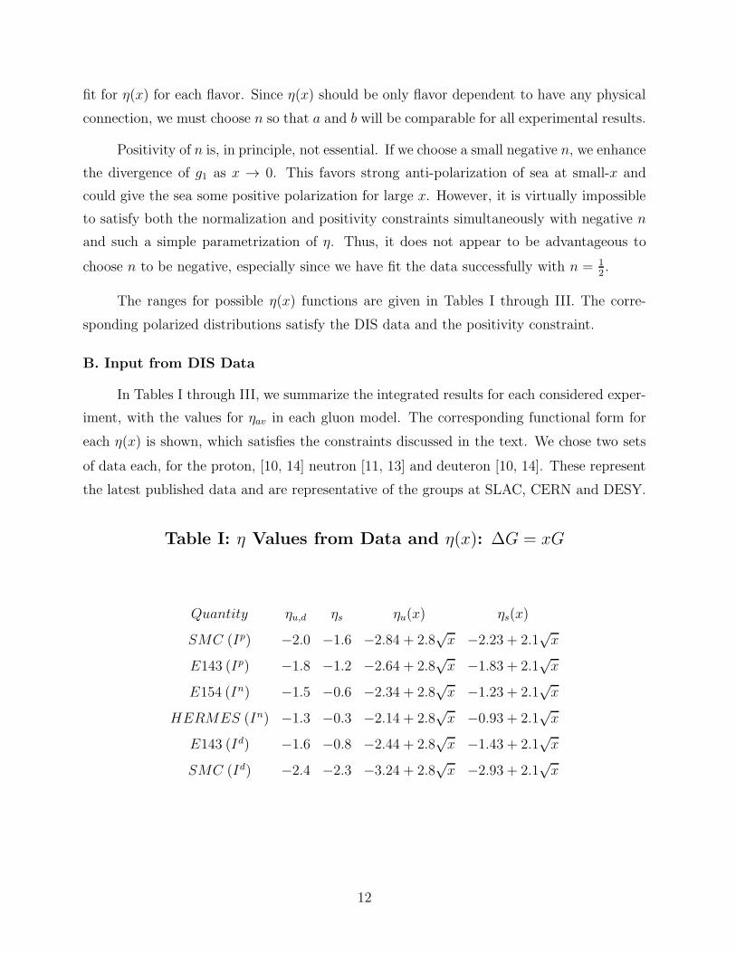
The ranges for possible η(x) functions are given in Tables I through III. The corre-

sponding polarized distributions satisfy the DIS data and the positivity constraint.

B. Input from DIS Data

In Tables I through III, we summarize the integrated results for each considered exper-

iment, with the values for ηav in each gluon model. The corresponding functional form for

each η(x) is shown, which satisfies the constraints discussed in the text. We chose two sets

of data each, for the proton, [10, 14] neutron [11, 13] and deuteron [10, 14]. These represent

the latest published data and are representative of the groups at SLAC, CERN and DESY.

Table I: η Values from Data and η(x): ∆G = xG

Quantity ηu,d ηs ηu(x) ηs(x)

SMC (Ip) −2.0 −1.6 −2.84 + 2.8√x −2.23 + 2.1

√x

E143 (Ip) −1.8 −1.2 −2.64 + 2.8√x −1.83 + 2.1

√x

E154 (In) −1.5 −0.6 −2.34 + 2.8√x −1.23 + 2.1

√x

HERMES (In) −1.3 −0.3 −2.14 + 2.8√x −0.93 + 2.1

√x

E143 (Id) −1.6 −0.8 −2.44 + 2.8√x −1.43 + 2.1

√x

SMC (Id) −2.4 −2.3 −3.24 + 2.8√x −2.93 + 2.1

√x

12

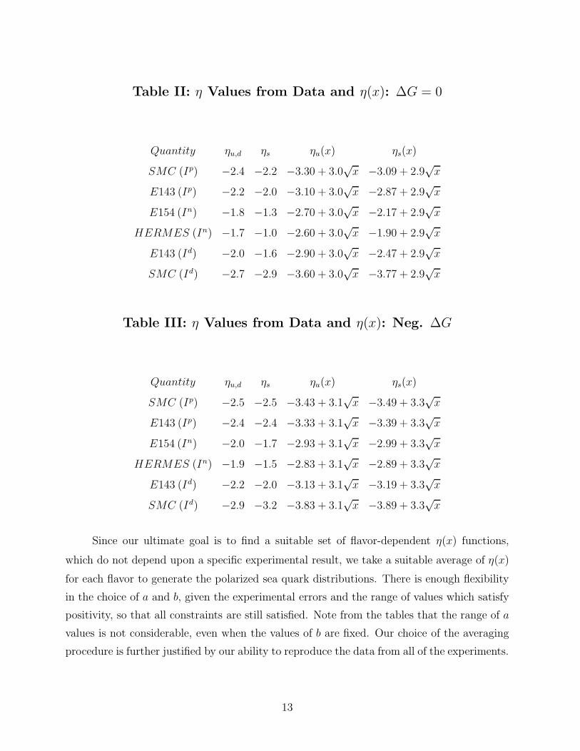
Table II: η Values from Data and η(x): ∆G = 0

Quantity ηu,d ηs ηu(x) ηs(x)

SMC (Ip) −2.4 −2.2 −3.30 + 3.0√x −3.09 + 2.9

√x

E143 (Ip) −2.2 −2.0 −3.10 + 3.0√x −2.87 + 2.9

√x

E154 (In) −1.8 −1.3 −2.70 + 3.0√x −2.17 + 2.9

√x

HERMES (In) −1.7 −1.0 −2.60 + 3.0√x −1.90 + 2.9

√x

E143 (Id) −2.0 −1.6 −2.90 + 3.0√x −2.47 + 2.9

√x

SMC (Id) −2.7 −2.9 −3.60 + 3.0√x −3.77 + 2.9

√x

Table III: η Values from Data and η(x): Neg. ∆G

Quantity ηu,d ηs ηu(x) ηs(x)

SMC (Ip) −2.5 −2.5 −3.43 + 3.1√x −3.49 + 3.3

√x

E143 (Ip) −2.4 −2.4 −3.33 + 3.1√x −3.39 + 3.3

√x

E154 (In) −2.0 −1.7 −2.93 + 3.1√x −2.99 + 3.3

√x

HERMES (In) −1.9 −1.5 −2.83 + 3.1√x −2.89 + 3.3

√x

E143 (Id) −2.2 −2.0 −3.13 + 3.1√x −3.19 + 3.3

√x

SMC (Id) −2.9 −3.2 −3.83 + 3.1√x −3.89 + 3.3

√x

Since our ultimate goal is to find a suitable set of flavor-dependent η(x) functions,

which do not depend upon a specific experimental result, we take a suitable average of η(x)

for each flavor to generate the polarized sea quark distributions. There is enough flexibility

in the choice of a and b, given the experimental errors and the range of values which satisfy

positivity, so that all constraints are still satisfied. Note from the tables that the range of a

values is not considerable, even when the values of b are fixed. Our choice of the averaging

procedure is further justified by our ability to reproduce the data from all of the experiments.

13

The resulting functions η(x) for each gluon model are:

Quantity ηu,d(x) ηs(x)

∆G = xG −2.49 + 2.8√x −1.67 + 2.1

√x

∆G = 0 −3.03 + 3.0√x −2.71 + 2.9

√x

∆G < 0 −3.25 + 3.1√x −3.31 + 3.3

√x

IV. Results and Discussion

A. Results for the Polarized Distributions

The polarized valence quark distributions are constructed with the assumptions made

in eqns. (2.1) and (2.3), with R0 determined by the BSR. The overall parametrization for

each of the polarized sea flavors, including the η(x) functions, the anomaly terms and the

up-down unpolarized asymmetry term can be written (with the CTEQ basis) in the form:

∆qi(x) = −Ax−0.143(1− x)8.041(1− B√x)

[

1 + 6.112x+ P (x)]

. (4.1)

The values for the variables in equation 4.1 are given for each flavor and each gluon model

in Table IV.

14

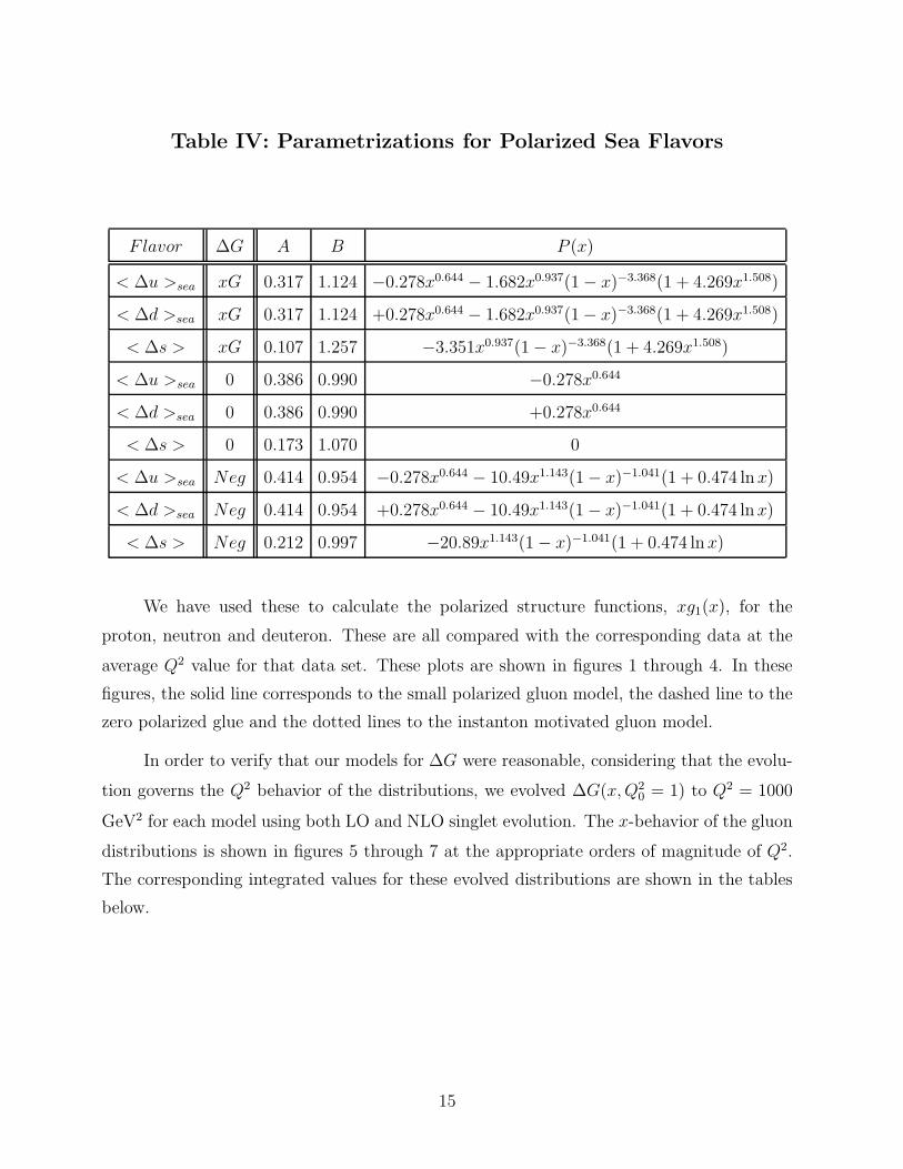
Table IV: Parametrizations for Polarized Sea Flavors

F lavor ∆G A B P (x)

< ∆u >sea xG 0.317 1.124 −0.278x0.644 − 1.682x0.937(1− x)−3.368(1 + 4.269x1.508)

< ∆d >sea xG 0.317 1.124 +0.278x0.644 − 1.682x0.937(1− x)−3.368(1 + 4.269x1.508)

< ∆s > xG 0.107 1.257 −3.351x0.937(1− x)−3.368(1 + 4.269x1.508)

< ∆u >sea 0 0.386 0.990 −0.278x0.644

< ∆d >sea 0 0.386 0.990 +0.278x0.644

< ∆s > 0 0.173 1.070 0

< ∆u >sea Neg 0.414 0.954 −0.278x0.644 − 10.49x1.143(1− x)−1.041(1 + 0.474 lnx)

< ∆d >sea Neg 0.414 0.954 +0.278x0.644 − 10.49x1.143(1− x)−1.041(1 + 0.474 lnx)

< ∆s > Neg 0.212 0.997 −20.89x1.143(1− x)−1.041(1 + 0.474 lnx)

We have used these to calculate the polarized structure functions, xg1(x), for the

proton, neutron and deuteron. These are all compared with the corresponding data at the

average Q2 value for that data set. These plots are shown in figures 1 through 4. In these

figures, the solid line corresponds to the small polarized gluon model, the dashed line to the

zero polarized glue and the dotted lines to the instanton motivated gluon model.

In order to verify that our models for ∆G were reasonable, considering that the evolu-

tion governs the Q2 behavior of the distributions, we evolved ∆G(x,Q20 = 1) to Q2 = 1000

GeV2 for each model using both LO and NLO singlet evolution. The x-behavior of the gluon

distributions is shown in figures 5 through 7 at the appropriate orders of magnitude of Q2.

The corresponding integrated values for these evolved distributions are shown in the tables

below.

15

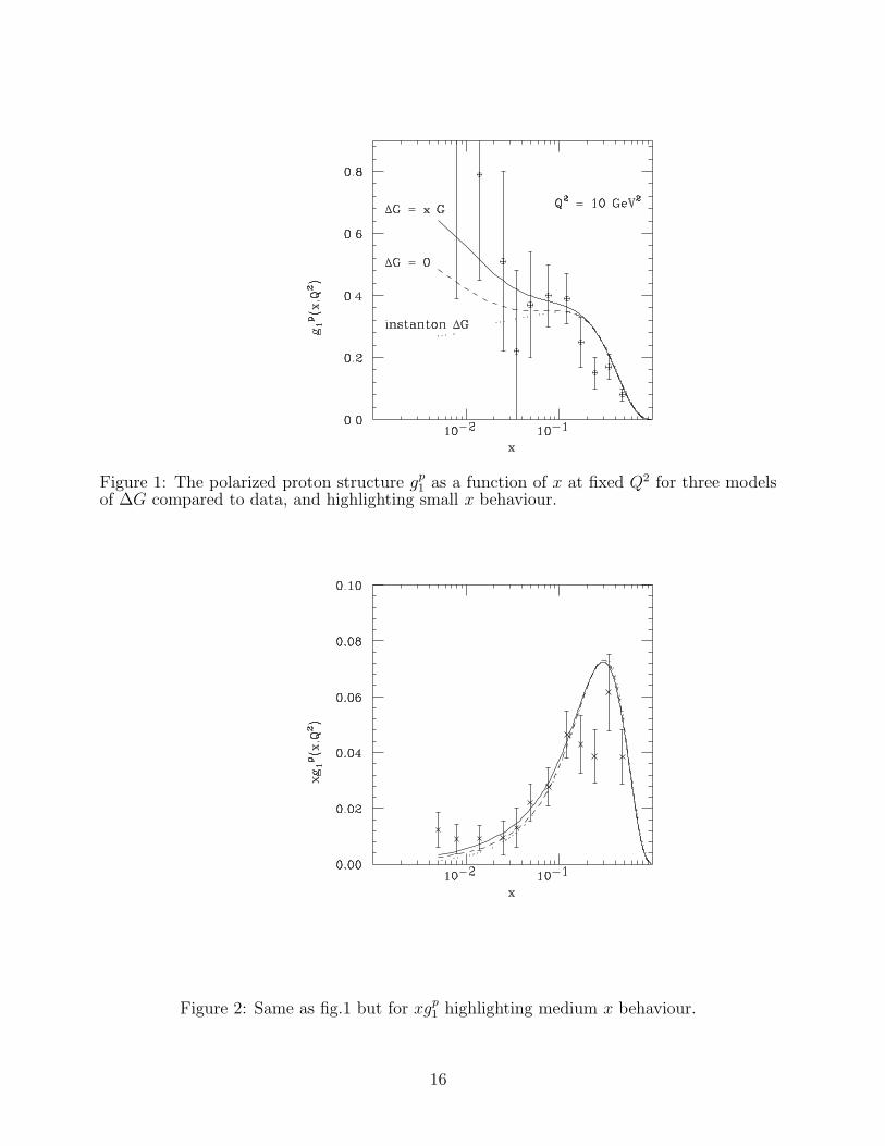
Figure 1: The polarized proton structure gp1 as a function of x at fixed Q2 for three modelsof ∆G compared to data, and highlighting small x behaviour.

Figure 2: Same as fig.1 but for xgp1 highlighting medium x behaviour.

16

Figure 3: The Polarized Neutron Distribution xgn1 as a function of x at Q2 = 10GeV 2

compared to data. The three curves are for three different gluon models (see text).

Figure 4: Same as fig.3 for gd1 .

17

Leading order polarized gluon evolution:∫ 1xmin

∆G dx

Q2(GeV 2) ∆G = xG ∆G = 0 Instanton

1 0.387 0.071 −0.076

10 0.651 0.107 +0.045

100 0.736 0.167 +0.118

1000 0.794 0.211 +0.182

Next-to-leading order polarized gluon evolution:∫ 1xmin

∆G dx

Q2(GeV 2) ∆G = xG ∆G = 0 Instanton

1 0.424 0.080 −0.082

10 0.653 0.119 +0.047

100 0.751 0.183 +0.130

1000 0.811 0.229 +0.190

For comparison with other models of the polarized quarks, we show the x-dependent

distributions of the valence and sea for each flavor in figures 8-11. The sea flavors are shown

for each gluon model. Note that our results compare favorably with other models. There

seems to be a general agreement about the shape of these distributions. Differences arise in

the actual numerical values of the integrated distributions. Both our x-dependent and our

integrated distributions have been constructed to satisfy all of the present data.

Physics Implications

1. All comparisons of our distributions with existing data are excellent, including Fig.

1, which shows g1, as opposed to xg1, accentuating the small-x behavior. The best overall

fits occur with the moderate glue (model 1). The zero glue model results are somewhat

better for the neutron, where the data are at lower average Q2 values. This is consistent

with the Q2 evolution of the polarized gluon distribution.

18

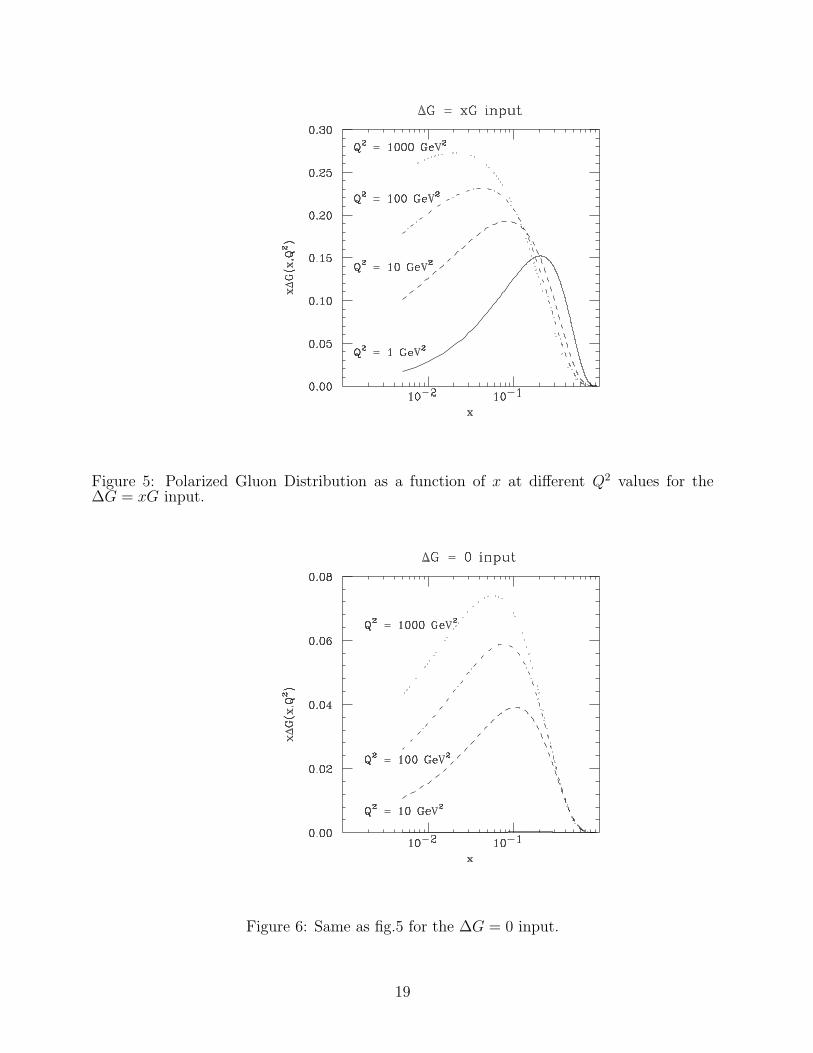
Figure 5: Polarized Gluon Distribution as a function of x at different Q2 values for the∆G = xG input.

Figure 6: Same as fig.5 for the ∆G = 0 input.

19

Figure 7: Same as fig.5 and fig.6 for the Instanton gluon input.

20

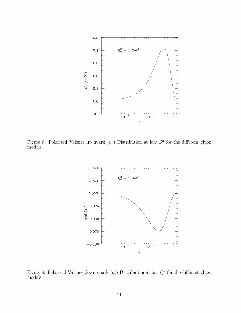
Figure 8: Polarized Valence up quark (uv) Distribution at low Q2 for the different gluonmodels.

Figure 9: Polarized Valence down quark (dv) Distribution at low Q2 for the different gluonmodels.

21

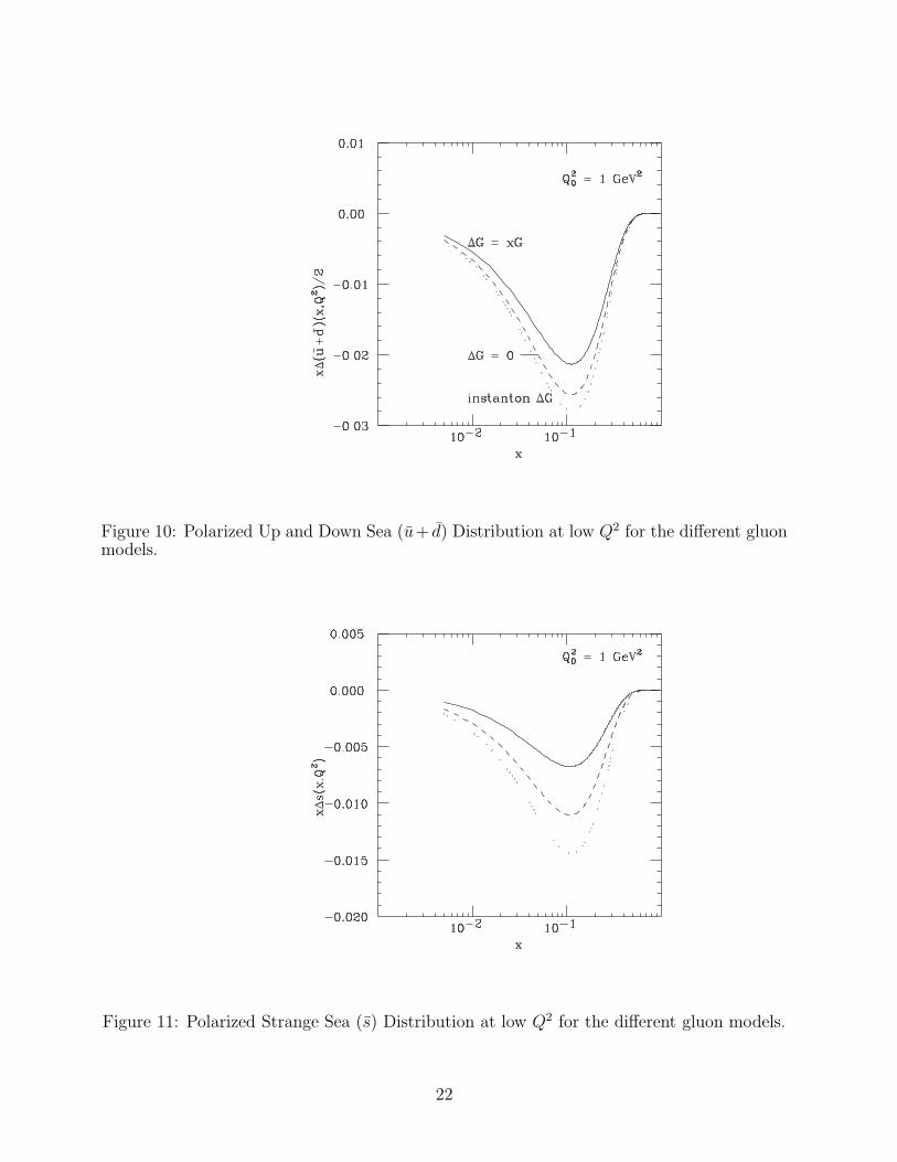
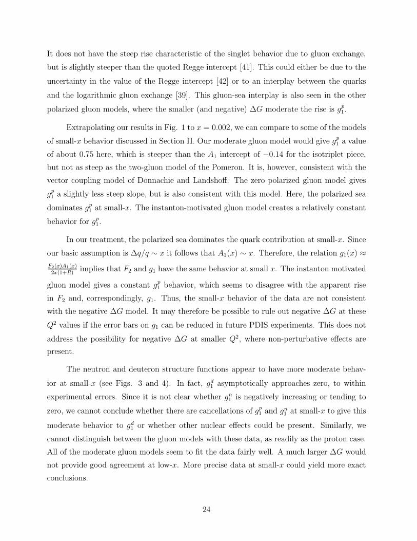
Figure 10: Polarized Up and Down Sea (u+ d) Distribution at low Q2 for the different gluonmodels.

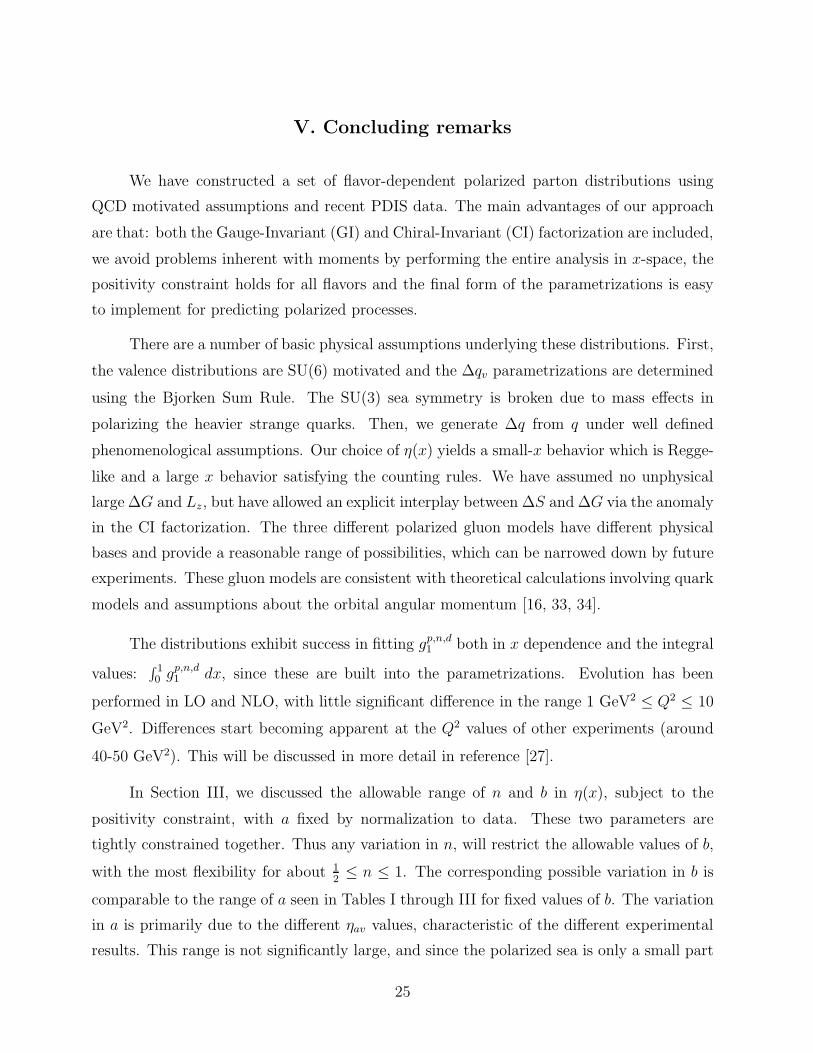
Figure 11: Polarized Strange Sea (s) Distribution at low Q2 for the different gluon models.

22

2. At small-x, the instanton gluon model predicts that gp1 decreases slightly. However,

considering the latitude in this distribution, it is consistent with a constant behavior. The

data appear to be rising in this x region, contrary to this implication. Since the data are at

average Q2 of 10 GeV2, this seems to indicate that the gluons are not negatively polarized

at such a relatively large Q2. This is consistent with the assumption that instantons are

dominant at smaller x and Q2 values and are likely not a major contributor to the polarized

glue at higher Q2 [35].

3. The polarized gluon distribution does not evolve as large as BFR predict, [4] even

with the moderate gluon model. Assumption of such large polarization at these lower Q2

values is unfounded. In fact, data from E704 at Fermilab indicate that it is likely more on

the order of the moderate or zero distribution. Even the NLO integrated polarized gluons

do not evolve significantly different from the LO distributions.

4. Our up and down valence distributions are comparable to others. Ours is motivated

from the physical SU(6) model with the BSR fixing the lone free parameter. It is compatible

with the u-valence domination at large x and has the appropriate x-dependent behavior at

all other x values.

5. The u and d polarized sea distributions are not highly dependent on the gluon model

used to generate them. However, the polarized strange sea is quite sensitive to the gluon

model and hence the anomaly term. This is discussed in more detail in reference [1].

6. The shape of the x-dependent polarized sea distributions agrees with the analysis

of Antonuccio, et. al.[36]. They exhibit Regge-like behavior at small-x and become slightly

positive at moderate x. Although it is not completely obvious from the figures, our sea

distributions remain negative until about x ∼ 0.3 and then turn slightly positive. This is

hidden by the dominance of the valence quarks in this kinematic range, but indicates a

consistency with physical expectations of the polarized sea.

B. Small-x Behavior

For the SMC proton data with the CTEQ unpolarized distributions and the positive

gluon model, we find at small x that: gp1 ∼ x−0.19. Phenomenologically, this is due to the

interplay between the sea distributions, with a ∆qi ∼ x−0.143 behavior in eqn. (3.1) and

the gluons in the model, dominated by xG ∼ x−0.206 at small-x in eqn. (2.9). Physically,

this is consistent with Regge behavior, characteristic of the iso-triplet contributions to g1.

23

It does not have the steep rise characteristic of the singlet behavior due to gluon exchange,

but is slightly steeper than the quoted Regge intercept [41]. This could either be due to the

uncertainty in the value of the Regge intercept [42] or to an interplay between the quarks

and the logarithmic gluon exchange [39]. This gluon-sea interplay is also seen in the other

polarized gluon models, where the smaller (and negative) ∆G moderate the rise is gp1.

Extrapolating our results in Fig. 1 to x = 0.002, we can compare to some of the models

of small-x behavior discussed in Section II. Our moderate gluon model would give gp1 a value

of about 0.75 here, which is steeper than the A1 intercept of −0.14 for the isotriplet piece,

but not as steep as the two-gluon model of the Pomeron. It is, however, consistent with the

vector coupling model of Donnachie and Landshoff. The zero polarized gluon model gives

gp1 a slightly less steep slope, but is also consistent with this model. Here, the polarized sea

dominates gp1 at small-x. The instanton-motivated gluon model creates a relatively constant

behavior for gp1.

In our treatment, the polarized sea dominates the quark contribution at small-x. Since

our basic assumption is ∆q/q ∼ x it follows that A1(x) ∼ x. Therefore, the relation g1(x) ≈F2(x)A1(x)2x(1+R)

implies that F2 and g1 have the same behavior at small x. The instanton motivated

gluon model gives a constant gp1 behavior, which seems to disagree with the apparent rise

in F2 and, correspondingly, g1. Thus, the small-x behavior of the data are not consistent

with the negative ∆G model. It may therefore be possible to rule out negative ∆G at these

Q2 values if the error bars on g1 can be reduced in future PDIS experiments. This does not

address the possibility for negative ∆G at smaller Q2, where non-perturbative effects are

present.

The neutron and deuteron structure functions appear to have more moderate behav-

ior at small-x (see Figs. 3 and 4). In fact, gd1 asymptotically approaches zero, to within

experimental errors. Since it is not clear whether gn1 is negatively increasing or tending to

zero, we cannot conclude whether there are cancellations of gp1 and gn1 at small-x to give this

moderate behavior to gd1 or whether other nuclear effects could be present. Similarly, we

cannot distinguish between the gluon models with these data, as readily as the proton case.

All of the moderate gluon models seem to fit the data fairly well. A much larger ∆G would

not provide good agreement at low-x. More precise data at small-x could yield more exact

conclusions.

24

V. Concluding remarks

We have constructed a set of flavor-dependent polarized parton distributions using

QCD motivated assumptions and recent PDIS data. The main advantages of our approach

are that: both the Gauge-Invariant (GI) and Chiral-Invariant (CI) factorization are included,

we avoid problems inherent with moments by performing the entire analysis in x-space, the

positivity constraint holds for all flavors and the final form of the parametrizations is easy

to implement for predicting polarized processes.

There are a number of basic physical assumptions underlying these distributions. First,

the valence distributions are SU(6) motivated and the ∆qv parametrizations are determined

using the Bjorken Sum Rule. The SU(3) sea symmetry is broken due to mass effects in

polarizing the heavier strange quarks. Then, we generate ∆q from q under well defined

phenomenological assumptions. Our choice of η(x) yields a small-x behavior which is Regge-

like and a large x behavior satisfying the counting rules. We have assumed no unphysical

large ∆G and Lz, but have allowed an explicit interplay between ∆S and ∆G via the anomaly

in the CI factorization. The three different polarized gluon models have different physical

bases and provide a reasonable range of possibilities, which can be narrowed down by future

experiments. These gluon models are consistent with theoretical calculations involving quark

models and assumptions about the orbital angular momentum [16, 33, 34].

The distributions exhibit success in fitting gp,n,d1 both in x dependence and the integral

values:∫ 10 gp,n,d1 dx, since these are built into the parametrizations. Evolution has been

performed in LO and NLO, with little significant difference in the range 1 GeV2 ≤ Q2 ≤ 10

GeV2. Differences start becoming apparent at the Q2 values of other experiments (around

40-50 GeV2). This will be discussed in more detail in reference [27].

In Section III, we discussed the allowable range of n and b in η(x), subject to the

positivity constraint, with a fixed by normalization to data. These two parameters are

tightly constrained together. Thus any variation in n, will restrict the allowable values of b,

with the most flexibility for about 12≤ n ≤ 1. The corresponding possible variation in b is

comparable to the range of a seen in Tables I through III for fixed values of b. The variation

in a is primarily due to the different ηav values, characteristic of the different experimental

results. This range is not significantly large, and since the polarized sea is only a small part

25

of g1, except perhaps at small-x, the differences are not significant to the overall results we

present here.

The results of gp1 at small-x imply that it may be possible to narrow down the gluon

size with more precise PDIS experiments at small-x. Such experiments are planned at SLAC

(E155) and DESY (HERMES). These would also refine the parametrizations by indicating

the behavior of gi1 at small-x. Comparisons of the x-dependent deuteron structure function

with the corresponding proton and neutron structure functions could provide insight into

possible nuclear effects, if they are significant. There are various possible experiments which

would provide a better indication of the size of the polarized gluon distribution. These

include: (1) one and two jet production in e−p and p−p collisions, [43, 44, 45, 46] (2) prompt

photon production [18, 47, 48, 49, 50], (3) charm production [51] and (4) pion production

[45]. Groups at RHIC (STAR), SLAC (E156), CERN (COMPASS) and DESY (HERA- ~N)

are planning to perform these experiments in the near future. For detailed explanations of

these experiments, see references [52] and [53]. We are presently calculating the appropriate

processes using the distributions and gluon models presented here [27].

Acknowledgement: One of us (G.P.R.) would like to thank P. Ratcliffe and D. Sivers

for useful discussions regarding the positivity constraint.

*References

[1] M. Goshtasbpour and G. P. Ramsey, Phys. Rev. D55, 1244 (1997)

[2] J. Ellis and M. Karliner, Phys. Lett. B341, 397 (1995)

[3] T.P. Cheng and L.-F. Li, Phys. Rev. Lett. 74, 2872 (1995), Phys. Rev. D57, 344 (1998)

[4] R.D. Ball, S. Forte and G. Rudolfi, Nucl. Phys. B444, 287 (1995); Nucl. Phys. B449,

680E (1995) and Nucl. Phys. B496, 337 (1997); G. Altarelli, R.D. Ball, S. Forte and

G. Rudolfi, hep-ph/9707276 and hep-ph/9803237

[5] T. Gehrmann and W. J. Stirling, Z. Phys. C65, 461 (1995)

[6] M. Gluck, E. Reya, M. Stratmann and W. Vogelsang, Phys. Rev. D53, 4775 (1996)

[7] J. Bartelski and S. Tatur, Z. Phys. C71, 595 (1996)

26

[8] D. DeFlorian, O.A. Sampayo and R. Sassot, hep-ph/9711440

[9] D. Indumathi, Z. Phys. C64, 439 (1994)

[10] K. Abe, et. al., Phys. Rev. Lett. 78, 815 (1997), Phys. Rev. D54, 6620 (1996), Phys.

Rev. Lett. 74, 346 (1995), Phys. Lett. B364, 61 (1995); P.L. Anthony, et. al., Phys.

Rev. Lett. 71, 959 (1993)

[11] K. Abe, et.al., Phys. Rev. Lett. 79, 26 (1997)

[12] P.L. Anthony, et. al., Phys. Rev. D54, 6620 (1996)

[13] K. Ackerstaff, et. al., Phys. Lett. B404, 383 (1997)

[14] B. Adeva, et. al., Phys. Lett. B320, 400 (1994); D. Adams, et. al., Phys. Lett. B329,

399 (1994), Phys. Lett. B357, 248 (1995) and Phys. Rev. D56, 5330 (1997)

[15] B. Adeva, et. al., Phys. Lett. B369, 93 (1996)

[16] S.J. Brodsky, M. Burkardt and I. Schmidt, Nucl. Phys. B441, 197 (1995)

[17] R. Carlitz and J. Kaur Phys. Rev. Lett. 38, 673 (1977); J. Kaur Nucl. Phys. B128, 219

(1977); F.E. Close, H. Osborn and A.M. Thomson, Nucl. Phys. B77, 281 (1974)

[18] J.-W. Qiu, G.P. Ramsey, D.G. Richards and D. Sivers, Phys. Rev. D41, 65 (1990)

[19] A.D. Martin, R.G. Roberts and W.J. Stirling, Phys. Lett. B387, 419 (1996)

[20] H.L. Lai, et. al., Phys. Rev. D55, 1280 (1997) and Phys. Rev. D51, 4763 (1996); W.-K.

Tung, hep-ph/9608293.

[21] F. Close and D. Sivers, Phys. Rev. Lett. 39, 1116 (1977)

[22] P. Chiapetta and J. Soffer, Phys. Rev. D31, 1019 (1985)

[23] S.A. Larin, F.V. Tkachev and J.A.M. Vermaseren, Phys. Rev. Lett. 66, 862 (1991) and

S.A. Larin and J.A.M. Vermaseren, Phys. Lett. B259, 345 (1991); A.L. Kataev and V.

Starshenko, CERN-TH-7198-94

[24] G. Rossi, Phys. Rev. D29 852, (1984)

27

[25] W. Vogelsang, Nucl. Phys. B475, 47 (1996); Phys. Rev. D54, 2023 (1996)

[26] S. Kumano and M. Mayama, Comput. Phys. Commun. 108, 38 (1998)

[27] L. E. Gordon and G. P. Ramsey, Work in Progress

[28] G. Bodwin and J.-W. Qiu, Phys. Rev. D41, 2755 (1990)

[29] Adler and W. Bardeen, Phys. Rev. 182, 1517 (1969)

[30] For a detailed discussion and comparison of these schemes, see H.-Y. Cheng, Int. J.

Mod. Phys., A11, 5109 (1996) and hep-ph/9712473

[31] A.V. Efremov and O.V. Teryaev, JINR Report E2-88-287 (1988); G. Altarelli and G.G.

Ross, Phys. Lett. B212, 391 (1988); R.D. Carlitz, J.C. Collins, and A.H. Mueller, Phys.

Lett. B214, 229 (1988)

[32] D.L. Adams, et. al., Phys. Lett. B336, 269 (1994); D.P. Grosnick, et. al., Phys. Rev.

D55, 1159 (1997)

[33] V. Barone, T. Calarco and A. Drago, hep-ph/9801281

[34] I. Balitsky and X. Ji, Phys. Rev. Lett. 79, 1225 (1997)

[35] N. Kochelev, AIP Conference Proceedings 407, 1997; DIS97, Chicago, IL, J. Repond

and D. Krakauer, Eds.

[36] F. Antonuccio, S.J. Brodsky, S. Dalley, Phys. Lett. B412, 104 (1997)

[37] F. Close and R.G. Roberts, Phys. Lett. B336, 257 (1994)

[38] A. Donnachie and P.V. Landshoff, Z. Phys. C61, 139 (1994)

[39] S.D. Bass and P.V. Landshoff, Phys. Lett. B336, 537 (1994)

[40] A.H. Mueller and T.L. Trueman, Phys. Rev. 160, 1306 (1967); L. Galfi, J. Kuti and A.

Pathos, Phys. Lett. B31, 465 (1970); F.E. Close and R.G. Roberts, Phys. Rev. Lett.

60, 1471 (1988)

[41] R.L. Heimann, Nucl. Phys. B64, 429 (1973)

28

[42] J. Ellis and M. Karliner, Phys. Lett. B213, 73 (1988)

[43] M. Stratmann and W. Vogelsang, Z. Phys. C74, 641 (1997)

[44] G.P. Ramsey, D. Richards and D. Sivers Phys. Rev. D37, 314 (1988)

[45] G.P. Ramsey and D. Sivers, Phys. Rev. D43, 2861 (1991)

[46] L.E. Gordon, Phys. Rev. D57, 235 (1998)

[47] L.E. Gordon and W. Vogelsang, Phys. Lett. B387, 629 (1996)

[48] L.E. Gordon and W. Vogelsang, Phys. Rev. D49, 170 (1994)

[49] A.P. Contogouris and Z. Merebashvili, Phys. Rev. D55, 2718 (1997)

[50] C. Coriano and L.E. Gordon, Phys. Rev. D49, 170 (1994) and

Phys. Rev. D54, 781 (1996)

[51] B. Baily, E.L. Berger and L.E. Gordon, Phys. Rev. D54, 1896 (1996)

[52] G.P. Ramsey, Prog. Part. Nucl. Physics, 39, 599 (1997) and Particle World, 4, No. 3

(1995)

[53] H. Bottcher, hep-ph/9712458

29