Embed Size (px)
Citation preview

ASAP 2020 Confirm
Developer/AnalystOperator’s Manual
V3.04
202-42811-01May 2010

Kalrez is a registered trademark of DuPont Dow Elastomers L.L.C.Teflon is a registered trademark of E.I. DuPont de Nemours CompanyWindows is a registered trademark of Microsoft Corporation
© Micromeritics Instrument Corporation 2004-2010. All rights reserved.
The software described in this manual is furnished under a license agreement and may be used or copied only in accordance with the terms of the agreement.
ASAP 2020 Confirm Table of Contents
TABLE OF CONTENTS
1. GENERAL INFORMATIONOrganization of the Operator’s Manual . . . . . . . . . . . . . . . . . . . . . . . . . . . . . . . . . . . . . . . . . . . . 1-1
Conventions . . . . . . . . . . . . . . . . . . . . . . . . . . . . . . . . . . . . . . . . . . . . . . . . . . . . . . . . . . . . . 1-2 Equipment Description . . . . . . . . . . . . . . . . . . . . . . . . . . . . . . . . . . . . . . . . . . . . . . . . . . . . . . . . 1-3
Gas Requirements . . . . . . . . . . . . . . . . . . . . . . . . . . . . . . . . . . . . . . . . . . . . . . . . . . . . . . . . 1-4Analysis Program . . . . . . . . . . . . . . . . . . . . . . . . . . . . . . . . . . . . . . . . . . . . . . . . . . . . . . . . . 1-4
Report System . . . . . . . . . . . . . . . . . . . . . . . . . . . . . . . . . . . . . . . . . . . . . . . . . . . . . . . 1-4Online Manual . . . . . . . . . . . . . . . . . . . . . . . . . . . . . . . . . . . . . . . . . . . . . . . . . . . . . . . . . . . . . . . 1-5
Using Bookmarks. . . . . . . . . . . . . . . . . . . . . . . . . . . . . . . . . . . . . . . . . . . . . . . . . . . . . . . . . 1-5Using the Table of Contents, Index, and other Links. . . . . . . . . . . . . . . . . . . . . . . . . . . . . . 1-7
Table of Contents . . . . . . . . . . . . . . . . . . . . . . . . . . . . . . . . . . . . . . . . . . . . . . . . . . . . . 1-7Index. . . . . . . . . . . . . . . . . . . . . . . . . . . . . . . . . . . . . . . . . . . . . . . . . . . . . . . . . . . . . . . 1-8Cross References . . . . . . . . . . . . . . . . . . . . . . . . . . . . . . . . . . . . . . . . . . . . . . . . . . . . . 1-8
Using the Find Command . . . . . . . . . . . . . . . . . . . . . . . . . . . . . . . . . . . . . . . . . . . . . . . . . . 1-9Printing . . . . . . . . . . . . . . . . . . . . . . . . . . . . . . . . . . . . . . . . . . . . . . . . . . . . . . . . . . . . . . . . . 1-10
Internet Access . . . . . . . . . . . . . . . . . . . . . . . . . . . . . . . . . . . . . . . . . . . . . . . . . . . . . . . . . . . . . . . 1-11Specifications . . . . . . . . . . . . . . . . . . . . . . . . . . . . . . . . . . . . . . . . . . . . . . . . . . . . . . . . . . . . . . . . 1-12
2. USER INTERFACEControls, Indicators, and Connectors . . . . . . . . . . . . . . . . . . . . . . . . . . . . . . . . . . . . . . . . . . . . . . 2-1
Front Panel . . . . . . . . . . . . . . . . . . . . . . . . . . . . . . . . . . . . . . . . . . . . . . . . . . . . . . . . . . . . . . 2-2Side Panel . . . . . . . . . . . . . . . . . . . . . . . . . . . . . . . . . . . . . . . . . . . . . . . . . . . . . . . . . . . . . . . 2-5
Upper . . . . . . . . . . . . . . . . . . . . . . . . . . . . . . . . . . . . . . . . . . . . . . . . . . . . . . . . . . . . . . 2-5Lower . . . . . . . . . . . . . . . . . . . . . . . . . . . . . . . . . . . . . . . . . . . . . . . . . . . . . . . . . . . . . . 2-6
Rear Panel . . . . . . . . . . . . . . . . . . . . . . . . . . . . . . . . . . . . . . . . . . . . . . . . . . . . . . . . . . . . . . 2-7Using the Software. . . . . . . . . . . . . . . . . . . . . . . . . . . . . . . . . . . . . . . . . . . . . . . . . . . . . . . . . . . . 2-8
Logging In . . . . . . . . . . . . . . . . . . . . . . . . . . . . . . . . . . . . . . . . . . . . . . . . . . . . . . . . . . . . . . 2-8Shortcut Menus . . . . . . . . . . . . . . . . . . . . . . . . . . . . . . . . . . . . . . . . . . . . . . . . . . . . . . . . . . 2-8Shortcut Keys . . . . . . . . . . . . . . . . . . . . . . . . . . . . . . . . . . . . . . . . . . . . . . . . . . . . . . . . . . . . 2-9Dialog Boxes . . . . . . . . . . . . . . . . . . . . . . . . . . . . . . . . . . . . . . . . . . . . . . . . . . . . . . . . . . . . 2-10Selecting Files . . . . . . . . . . . . . . . . . . . . . . . . . . . . . . . . . . . . . . . . . . . . . . . . . . . . . . . . . . . 2-12
Menu Structure. . . . . . . . . . . . . . . . . . . . . . . . . . . . . . . . . . . . . . . . . . . . . . . . . . . . . . . . . . . . . . . 2-14Windows Menu . . . . . . . . . . . . . . . . . . . . . . . . . . . . . . . . . . . . . . . . . . . . . . . . . . . . . . . . . . 2-15Help Menu . . . . . . . . . . . . . . . . . . . . . . . . . . . . . . . . . . . . . . . . . . . . . . . . . . . . . . . . . . . . . . 2-16
3. OPERATIONAL PROCEDURESCreating File Templates . . . . . . . . . . . . . . . . . . . . . . . . . . . . . . . . . . . . . . . . . . . . . . . . . . . . . . . . 3-1Creating Parameter Files . . . . . . . . . . . . . . . . . . . . . . . . . . . . . . . . . . . . . . . . . . . . . . . . . . . . . . . 3-3
Sample Tube. . . . . . . . . . . . . . . . . . . . . . . . . . . . . . . . . . . . . . . . . . . . . . . . . . . . . . . . . . . . . 3-3Degas Conditions . . . . . . . . . . . . . . . . . . . . . . . . . . . . . . . . . . . . . . . . . . . . . . . . . . . . . . . . . 3-4Analysis Conditions . . . . . . . . . . . . . . . . . . . . . . . . . . . . . . . . . . . . . . . . . . . . . . . . . . . . . . . 3-5
May 2010 i
Table of Contents ASAP2020 Confirm
Adsorptive Properties . . . . . . . . . . . . . . . . . . . . . . . . . . . . . . . . . . . . . . . . . . . . . . . . . . . . . . 3-7Report Options . . . . . . . . . . . . . . . . . . . . . . . . . . . . . . . . . . . . . . . . . . . . . . . . . . . . . . . . . . . 3-8
Creating a Sample File . . . . . . . . . . . . . . . . . . . . . . . . . . . . . . . . . . . . . . . . . . . . . . . . . . . . . . . . . 3-10Analyst . . . . . . . . . . . . . . . . . . . . . . . . . . . . . . . . . . . . . . . . . . . . . . . . . . . . . . . . . . . . . . . . . 3-10Developer . . . . . . . . . . . . . . . . . . . . . . . . . . . . . . . . . . . . . . . . . . . . . . . . . . . . . . . . . . . . . . . 3-11
Preparing Samples . . . . . . . . . . . . . . . . . . . . . . . . . . . . . . . . . . . . . . . . . . . . . . . . . . . . . . . . . . . . 3-13Choosing Sample Tubes . . . . . . . . . . . . . . . . . . . . . . . . . . . . . . . . . . . . . . . . . . . . . . . . . . . . 3-13Cleaning and Labeling Sample Tubes . . . . . . . . . . . . . . . . . . . . . . . . . . . . . . . . . . . . . . . . . 3-14Determining Amount of Sample to Use . . . . . . . . . . . . . . . . . . . . . . . . . . . . . . . . . . . . . . . . 3-18Determining the Mass of the Sample . . . . . . . . . . . . . . . . . . . . . . . . . . . . . . . . . . . . . . . . . . 3-18Degassing the Sample. . . . . . . . . . . . . . . . . . . . . . . . . . . . . . . . . . . . . . . . . . . . . . . . . . . . . . 3-20Transferring the Degassed Sample to the Analysis Port. . . . . . . . . . . . . . . . . . . . . . . . . . . . 3-22
Installing Dewars . . . . . . . . . . . . . . . . . . . . . . . . . . . . . . . . . . . . . . . . . . . . . . . . . . . . . . . . . . . . . 3-24Precautions . . . . . . . . . . . . . . . . . . . . . . . . . . . . . . . . . . . . . . . . . . . . . . . . . . . . . . . . . . . . . . 3-24Cold Trap Dewar . . . . . . . . . . . . . . . . . . . . . . . . . . . . . . . . . . . . . . . . . . . . . . . . . . . . . . . . . 3-25Analysis Dewar. . . . . . . . . . . . . . . . . . . . . . . . . . . . . . . . . . . . . . . . . . . . . . . . . . . . . . . . . . . 3-26
Performing an Analysis . . . . . . . . . . . . . . . . . . . . . . . . . . . . . . . . . . . . . . . . . . . . . . . . . . . . . . . . 3-27Printing File Contents . . . . . . . . . . . . . . . . . . . . . . . . . . . . . . . . . . . . . . . . . . . . . . . . . . . . . . . . . . 3-29Listing File Statistics . . . . . . . . . . . . . . . . . . . . . . . . . . . . . . . . . . . . . . . . . . . . . . . . . . . . . . . . . . 3-30Importing Sample and Parameter Files. . . . . . . . . . . . . . . . . . . . . . . . . . . . . . . . . . . . . . . . . . . . . 3-31Exporting a Sample Information File . . . . . . . . . . . . . . . . . . . . . . . . . . . . . . . . . . . . . . . . . . . . . . 3-32Generating Graph Overlays . . . . . . . . . . . . . . . . . . . . . . . . . . . . . . . . . . . . . . . . . . . . . . . . . . . . . 3-33
Multiple Samples Overlay . . . . . . . . . . . . . . . . . . . . . . . . . . . . . . . . . . . . . . . . . . . . . . . . . . 3-34Multiple Graphs Overlay . . . . . . . . . . . . . . . . . . . . . . . . . . . . . . . . . . . . . . . . . . . . . . . . . . . 3-37
4. FILE MENUDescription . . . . . . . . . . . . . . . . . . . . . . . . . . . . . . . . . . . . . . . . . . . . . . . . . . . . . . . . . . . . . . . . . . 4-1New. . . . . . . . . . . . . . . . . . . . . . . . . . . . . . . . . . . . . . . . . . . . . . . . . . . . . . . . . . . . . . . . . . . . . . . . 4-3
Sample Information . . . . . . . . . . . . . . . . . . . . . . . . . . . . . . . . . . . . . . . . . . . . . . . . . . . . . . . 4-4Analyst . . . . . . . . . . . . . . . . . . . . . . . . . . . . . . . . . . . . . . . . . . . . . . . . . . . . . . . . . . . . . 4-4Developer . . . . . . . . . . . . . . . . . . . . . . . . . . . . . . . . . . . . . . . . . . . . . . . . . . . . . . . . . . . 4-7
Sample Tube . . . . . . . . . . . . . . . . . . . . . . . . . . . . . . . . . . . . . . . . . . . . . . . . . . . . . . . . . . . . . 4-10Degas Conditions . . . . . . . . . . . . . . . . . . . . . . . . . . . . . . . . . . . . . . . . . . . . . . . . . . . . . . . . . 4-12Analysis Conditions . . . . . . . . . . . . . . . . . . . . . . . . . . . . . . . . . . . . . . . . . . . . . . . . . . . . . . . 4-15Adsorptive Properties . . . . . . . . . . . . . . . . . . . . . . . . . . . . . . . . . . . . . . . . . . . . . . . . . . . . . . 4-27Report Options . . . . . . . . . . . . . . . . . . . . . . . . . . . . . . . . . . . . . . . . . . . . . . . . . . . . . . . . . . . 4-30
Summary Report . . . . . . . . . . . . . . . . . . . . . . . . . . . . . . . . . . . . . . . . . . . . . . . . . . . . . . 4-34Isotherm Report Options. . . . . . . . . . . . . . . . . . . . . . . . . . . . . . . . . . . . . . . . . . . . . . . . 4-36BET/Langmuir Surface Area Report Options. . . . . . . . . . . . . . . . . . . . . . . . . . . . . . . . 4-39Freundlich Isotherm . . . . . . . . . . . . . . . . . . . . . . . . . . . . . . . . . . . . . . . . . . . . . . . . . . . 4-42Temkin Isotherm. . . . . . . . . . . . . . . . . . . . . . . . . . . . . . . . . . . . . . . . . . . . . . . . . . . . . . 4-44t-Plot Report Options . . . . . . . . . . . . . . . . . . . . . . . . . . . . . . . . . . . . . . . . . . . . . . . . . . 4-46Alpha-S Plot . . . . . . . . . . . . . . . . . . . . . . . . . . . . . . . . . . . . . . . . . . . . . . . . . . . . . . . . . 4-52f-Ratio Plot . . . . . . . . . . . . . . . . . . . . . . . . . . . . . . . . . . . . . . . . . . . . . . . . . . . . . . . . . . 4-54BJH Adsorption/Desorption Report Options . . . . . . . . . . . . . . . . . . . . . . . . . . . . . . . . 4-56Dollimore-Heal Adsorption/Desorption Report Options . . . . . . . . . . . . . . . . . . . . . . . 4-64Horvath-Kawazoe Report Options . . . . . . . . . . . . . . . . . . . . . . . . . . . . . . . . . . . . . . . . 4-65DFT Pore Size. . . . . . . . . . . . . . . . . . . . . . . . . . . . . . . . . . . . . . . . . . . . . . . . . . . . . . . . 4-71
ii May 2010
ASAP 2020 Confirm Table of Contents
DFT Surface Energy. . . . . . . . . . . . . . . . . . . . . . . . . . . . . . . . . . . . . . . . . . . . . . . . . . . 4-74Dubinin Report Options . . . . . . . . . . . . . . . . . . . . . . . . . . . . . . . . . . . . . . . . . . . . . . . . 4-75MP-Method Report Options. . . . . . . . . . . . . . . . . . . . . . . . . . . . . . . . . . . . . . . . . . . . . 4-80Options Report . . . . . . . . . . . . . . . . . . . . . . . . . . . . . . . . . . . . . . . . . . . . . . . . . . . . . . . 4-84Sample Log Report. . . . . . . . . . . . . . . . . . . . . . . . . . . . . . . . . . . . . . . . . . . . . . . . . . . . 4-84Validation Report . . . . . . . . . . . . . . . . . . . . . . . . . . . . . . . . . . . . . . . . . . . . . . . . . . . . . 4-85
Collected/Entered Data . . . . . . . . . . . . . . . . . . . . . . . . . . . . . . . . . . . . . . . . . . . . . . . . . . . . 4-86Open . . . . . . . . . . . . . . . . . . . . . . . . . . . . . . . . . . . . . . . . . . . . . . . . . . . . . . . . . . . . . . . . . . . . . . . 4-88
Sample Information File. . . . . . . . . . . . . . . . . . . . . . . . . . . . . . . . . . . . . . . . . . . . . . . . . . . . 4-88Analyst . . . . . . . . . . . . . . . . . . . . . . . . . . . . . . . . . . . . . . . . . . . . . . . . . . . . . . . . . . . . . 4-90Developer . . . . . . . . . . . . . . . . . . . . . . . . . . . . . . . . . . . . . . . . . . . . . . . . . . . . . . . . . . . 4-91
Templates . . . . . . . . . . . . . . . . . . . . . . . . . . . . . . . . . . . . . . . . . . . . . . . . . . . . . . . . . . . . . . . 4-91Parameter Files. . . . . . . . . . . . . . . . . . . . . . . . . . . . . . . . . . . . . . . . . . . . . . . . . . . . . . . . . . . 4-92
Save . . . . . . . . . . . . . . . . . . . . . . . . . . . . . . . . . . . . . . . . . . . . . . . . . . . . . . . . . . . . . . . . . . . . . . . 4-93Save As. . . . . . . . . . . . . . . . . . . . . . . . . . . . . . . . . . . . . . . . . . . . . . . . . . . . . . . . . . . . . . . . . . . . . 4-93Save As Template . . . . . . . . . . . . . . . . . . . . . . . . . . . . . . . . . . . . . . . . . . . . . . . . . . . . . . . . . . . . 4-95Save All . . . . . . . . . . . . . . . . . . . . . . . . . . . . . . . . . . . . . . . . . . . . . . . . . . . . . . . . . . . . . . . . . . . . 4-95Close. . . . . . . . . . . . . . . . . . . . . . . . . . . . . . . . . . . . . . . . . . . . . . . . . . . . . . . . . . . . . . . . . . . . . . . 4-96Close All. . . . . . . . . . . . . . . . . . . . . . . . . . . . . . . . . . . . . . . . . . . . . . . . . . . . . . . . . . . . . . . . . . . . 4-96Print . . . . . . . . . . . . . . . . . . . . . . . . . . . . . . . . . . . . . . . . . . . . . . . . . . . . . . . . . . . . . . . . . . . . . . . 4-97List . . . . . . . . . . . . . . . . . . . . . . . . . . . . . . . . . . . . . . . . . . . . . . . . . . . . . . . . . . . . . . . . . . . . . . . . 4-99Import. . . . . . . . . . . . . . . . . . . . . . . . . . . . . . . . . . . . . . . . . . . . . . . . . . . . . . . . . . . . . . . . . . . . . . 4-100Export. . . . . . . . . . . . . . . . . . . . . . . . . . . . . . . . . . . . . . . . . . . . . . . . . . . . . . . . . . . . . . . . . . . . . . 4-101Convert. . . . . . . . . . . . . . . . . . . . . . . . . . . . . . . . . . . . . . . . . . . . . . . . . . . . . . . . . . . . . . . . . . . . . 4-102Log In . . . . . . . . . . . . . . . . . . . . . . . . . . . . . . . . . . . . . . . . . . . . . . . . . . . . . . . . . . . . . . . . . . . . . . 4-103Log Out . . . . . . . . . . . . . . . . . . . . . . . . . . . . . . . . . . . . . . . . . . . . . . . . . . . . . . . . . . . . . . . . . . . . 4-103Exit . . . . . . . . . . . . . . . . . . . . . . . . . . . . . . . . . . . . . . . . . . . . . . . . . . . . . . . . . . . . . . . . . . . . . . . . 4-104
5. UNIT MENUDescription . . . . . . . . . . . . . . . . . . . . . . . . . . . . . . . . . . . . . . . . . . . . . . . . . . . . . . . . . . . . . . . . . . 5-1Sample Analysis. . . . . . . . . . . . . . . . . . . . . . . . . . . . . . . . . . . . . . . . . . . . . . . . . . . . . . . . . . . . . . 5-3Start Degas . . . . . . . . . . . . . . . . . . . . . . . . . . . . . . . . . . . . . . . . . . . . . . . . . . . . . . . . . . . . . . . . . . 5-8Enable Manual Control . . . . . . . . . . . . . . . . . . . . . . . . . . . . . . . . . . . . . . . . . . . . . . . . . . . . . . . . 5-9Show Instrument Schematic. . . . . . . . . . . . . . . . . . . . . . . . . . . . . . . . . . . . . . . . . . . . . . . . . . . . . 5-12Show Status . . . . . . . . . . . . . . . . . . . . . . . . . . . . . . . . . . . . . . . . . . . . . . . . . . . . . . . . . . . . . . . . . 5-13Show Instrument Log. . . . . . . . . . . . . . . . . . . . . . . . . . . . . . . . . . . . . . . . . . . . . . . . . . . . . . . . . . 5-14Unit Configuration . . . . . . . . . . . . . . . . . . . . . . . . . . . . . . . . . . . . . . . . . . . . . . . . . . . . . . . . . . . . 5-16Diagnostics. . . . . . . . . . . . . . . . . . . . . . . . . . . . . . . . . . . . . . . . . . . . . . . . . . . . . . . . . . . . . . . . . . 5-18Calibration . . . . . . . . . . . . . . . . . . . . . . . . . . . . . . . . . . . . . . . . . . . . . . . . . . . . . . . . . . . . . . . . . . 5-19
Vacuum Gauge. . . . . . . . . . . . . . . . . . . . . . . . . . . . . . . . . . . . . . . . . . . . . . . . . . . . . . . . . . . 5-19Pressure Zero . . . . . . . . . . . . . . . . . . . . . . . . . . . . . . . . . . . . . . . . . . . . . . . . . . . . . . . . . . . . 5-19Pressure Scale. . . . . . . . . . . . . . . . . . . . . . . . . . . . . . . . . . . . . . . . . . . . . . . . . . . . . . . . . . . . 5-20Temperature . . . . . . . . . . . . . . . . . . . . . . . . . . . . . . . . . . . . . . . . . . . . . . . . . . . . . . . . . . . . . 5-20Volume . . . . . . . . . . . . . . . . . . . . . . . . . . . . . . . . . . . . . . . . . . . . . . . . . . . . . . . . . . . . . . . . . 5-21Save to File. . . . . . . . . . . . . . . . . . . . . . . . . . . . . . . . . . . . . . . . . . . . . . . . . . . . . . . . . . . . . . 5-23Load from File . . . . . . . . . . . . . . . . . . . . . . . . . . . . . . . . . . . . . . . . . . . . . . . . . . . . . . . . . . . 5-23
Degas . . . . . . . . . . . . . . . . . . . . . . . . . . . . . . . . . . . . . . . . . . . . . . . . . . . . . . . . . . . . . . . . . . . . . . 5-24Enable Manual Control . . . . . . . . . . . . . . . . . . . . . . . . . . . . . . . . . . . . . . . . . . . . . . . . . . . . 5-24
May 2010 iii
Table of Contents ASAP2020 Confirm
Show Instrument Schematic . . . . . . . . . . . . . . . . . . . . . . . . . . . . . . . . . . . . . . . . . . . . . . . . . 5-25Show Status. . . . . . . . . . . . . . . . . . . . . . . . . . . . . . . . . . . . . . . . . . . . . . . . . . . . . . . . . . . . . . 5-26Calibrate Pressure Zero. . . . . . . . . . . . . . . . . . . . . . . . . . . . . . . . . . . . . . . . . . . . . . . . . . . . . 5-27Calibrate Pressure Scale . . . . . . . . . . . . . . . . . . . . . . . . . . . . . . . . . . . . . . . . . . . . . . . . . . . . 5-27Calibrate Vacuum Gauge . . . . . . . . . . . . . . . . . . . . . . . . . . . . . . . . . . . . . . . . . . . . . . . . . . . 5-28Calibrate Servo . . . . . . . . . . . . . . . . . . . . . . . . . . . . . . . . . . . . . . . . . . . . . . . . . . . . . . . . . . . 5-28
Service Test . . . . . . . . . . . . . . . . . . . . . . . . . . . . . . . . . . . . . . . . . . . . . . . . . . . . . . . . . . . . . . . . . 5-29
6. REPORTS MENUDescription . . . . . . . . . . . . . . . . . . . . . . . . . . . . . . . . . . . . . . . . . . . . . . . . . . . . . . . . . . . . . . . . . . 6-1Start Report. . . . . . . . . . . . . . . . . . . . . . . . . . . . . . . . . . . . . . . . . . . . . . . . . . . . . . . . . . . . . . . . . . 6-3Close Reports . . . . . . . . . . . . . . . . . . . . . . . . . . . . . . . . . . . . . . . . . . . . . . . . . . . . . . . . . . . . . . . . 6-5Open Report . . . . . . . . . . . . . . . . . . . . . . . . . . . . . . . . . . . . . . . . . . . . . . . . . . . . . . . . . . . . . . . . . 6-5SPC Report Options . . . . . . . . . . . . . . . . . . . . . . . . . . . . . . . . . . . . . . . . . . . . . . . . . . . . . . . . . . . 6-6Regression Report. . . . . . . . . . . . . . . . . . . . . . . . . . . . . . . . . . . . . . . . . . . . . . . . . . . . . . . . . . . . . 6-7Control Chart . . . . . . . . . . . . . . . . . . . . . . . . . . . . . . . . . . . . . . . . . . . . . . . . . . . . . . . . . . . . . . . . 6-11Heat of Adsorption . . . . . . . . . . . . . . . . . . . . . . . . . . . . . . . . . . . . . . . . . . . . . . . . . . . . . . . . . . . . 6-14Rate of Adsorption (ROA) . . . . . . . . . . . . . . . . . . . . . . . . . . . . . . . . . . . . . . . . . . . . . . . . . . . . . . 6-17Printed Reports . . . . . . . . . . . . . . . . . . . . . . . . . . . . . . . . . . . . . . . . . . . . . . . . . . . . . . . . . . . . . . . 6-18
Header . . . . . . . . . . . . . . . . . . . . . . . . . . . . . . . . . . . . . . . . . . . . . . . . . . . . . . . . . . . . . . . . . . 6-18Onscreen Reports . . . . . . . . . . . . . . . . . . . . . . . . . . . . . . . . . . . . . . . . . . . . . . . . . . . . . . . . . . . . . 6-18
Tool Bar . . . . . . . . . . . . . . . . . . . . . . . . . . . . . . . . . . . . . . . . . . . . . . . . . . . . . . . . . . . . . . . . 6-19Shortcut Menus . . . . . . . . . . . . . . . . . . . . . . . . . . . . . . . . . . . . . . . . . . . . . . . . . . . . . . . . . . . 6-23
Tabular Reports. . . . . . . . . . . . . . . . . . . . . . . . . . . . . . . . . . . . . . . . . . . . . . . . . . . . . . . 6-23Graphs . . . . . . . . . . . . . . . . . . . . . . . . . . . . . . . . . . . . . . . . . . . . . . . . . . . . . . . . . . . . . . 6-24
Zoom Feature . . . . . . . . . . . . . . . . . . . . . . . . . . . . . . . . . . . . . . . . . . . . . . . . . . . . . . . . . . . . 6-26Axis Cross Hair. . . . . . . . . . . . . . . . . . . . . . . . . . . . . . . . . . . . . . . . . . . . . . . . . . . . . . . . . . . 6-27
Report Examples. . . . . . . . . . . . . . . . . . . . . . . . . . . . . . . . . . . . . . . . . . . . . . . . . . . . . . . . . . . . . . 6-27Tabular Report . . . . . . . . . . . . . . . . . . . . . . . . . . . . . . . . . . . . . . . . . . . . . . . . . . . . . . . . . . . 6-28Isotherm Plot. . . . . . . . . . . . . . . . . . . . . . . . . . . . . . . . . . . . . . . . . . . . . . . . . . . . . . . . . . . . . 6-29t-Plot . . . . . . . . . . . . . . . . . . . . . . . . . . . . . . . . . . . . . . . . . . . . . . . . . . . . . . . . . . . . . . . . . . . 6-30BET Surface Area Plot . . . . . . . . . . . . . . . . . . . . . . . . . . . . . . . . . . . . . . . . . . . . . . . . . . . . . 6-31BJH Adsorption . . . . . . . . . . . . . . . . . . . . . . . . . . . . . . . . . . . . . . . . . . . . . . . . . . . . . . . . . . 6-32Summary Report . . . . . . . . . . . . . . . . . . . . . . . . . . . . . . . . . . . . . . . . . . . . . . . . . . . . . . . . . . 6-33Options Report . . . . . . . . . . . . . . . . . . . . . . . . . . . . . . . . . . . . . . . . . . . . . . . . . . . . . . . . . . . 6-34Sample Log Report . . . . . . . . . . . . . . . . . . . . . . . . . . . . . . . . . . . . . . . . . . . . . . . . . . . . . . . . 6-35
7. OPTIONS MENUDescription . . . . . . . . . . . . . . . . . . . . . . . . . . . . . . . . . . . . . . . . . . . . . . . . . . . . . . . . . . . . . . . . . . 7-1Add Archive Location . . . . . . . . . . . . . . . . . . . . . . . . . . . . . . . . . . . . . . . . . . . . . . . . . . . . . . . . . 7-2Edit Labels . . . . . . . . . . . . . . . . . . . . . . . . . . . . . . . . . . . . . . . . . . . . . . . . . . . . . . . . . . . . . . . . . . 7-3Update File List . . . . . . . . . . . . . . . . . . . . . . . . . . . . . . . . . . . . . . . . . . . . . . . . . . . . . . . . . . . . . . 7-4Units . . . . . . . . . . . . . . . . . . . . . . . . . . . . . . . . . . . . . . . . . . . . . . . . . . . . . . . . . . . . . . . . . . . . . . . 7-4Graph Grid Lines . . . . . . . . . . . . . . . . . . . . . . . . . . . . . . . . . . . . . . . . . . . . . . . . . . . . . . . . . . . . . 7-5Live Graph . . . . . . . . . . . . . . . . . . . . . . . . . . . . . . . . . . . . . . . . . . . . . . . . . . . . . . . . . . . . . . . . . . 7-6Service Test Mode . . . . . . . . . . . . . . . . . . . . . . . . . . . . . . . . . . . . . . . . . . . . . . . . . . . . . . . . . . . . 7-6
iv May 2010
ASAP 2020 Confirm Table of Contents
8. TROUBLESHOOTING AND MAINTENANCE Troubleshooting . . . . . . . . . . . . . . . . . . . . . . . . . . . . . . . . . . . . . . . . . . . . . . . . . . . . . . . . . . . . . . 8-1Preventive Maintenance . . . . . . . . . . . . . . . . . . . . . . . . . . . . . . . . . . . . . . . . . . . . . . . . . . . . . . . . 8-3
Lubricating the Elevator Screw . . . . . . . . . . . . . . . . . . . . . . . . . . . . . . . . . . . . . . . . . . . . . . 8-4Checking the Analysis Port Dewar . . . . . . . . . . . . . . . . . . . . . . . . . . . . . . . . . . . . . . . . . . . 8-4Replacing the Sample Tube O-ring . . . . . . . . . . . . . . . . . . . . . . . . . . . . . . . . . . . . . . . . . . . 8-5Replacing the Port Filters. . . . . . . . . . . . . . . . . . . . . . . . . . . . . . . . . . . . . . . . . . . . . . . . . . . 8-7
Analysis Port . . . . . . . . . . . . . . . . . . . . . . . . . . . . . . . . . . . . . . . . . . . . . . . . . . . . . . . . 8-7Degas Port . . . . . . . . . . . . . . . . . . . . . . . . . . . . . . . . . . . . . . . . . . . . . . . . . . . . . . . . . . 8-8
Replacing the Vacuum Pump Exhaust Filter . . . . . . . . . . . . . . . . . . . . . . . . . . . . . . . . . . . . 8-8Inspecting and Changing Vacuum Pump Fluid . . . . . . . . . . . . . . . . . . . . . . . . . . . . . . . . . . 8-10
Inspecting Fluid . . . . . . . . . . . . . . . . . . . . . . . . . . . . . . . . . . . . . . . . . . . . . . . . . . . . . . 8-10Changing Fluid . . . . . . . . . . . . . . . . . . . . . . . . . . . . . . . . . . . . . . . . . . . . . . . . . . . . . . . 8-10
Replacing the Alumina in the Oil Vapor Traps . . . . . . . . . . . . . . . . . . . . . . . . . . . . . . . . . . 8-12Cleaning the Cold Trap Tubes . . . . . . . . . . . . . . . . . . . . . . . . . . . . . . . . . . . . . . . . . . . . . . . 8-15Calibrating the Manifold Temperature Sensor. . . . . . . . . . . . . . . . . . . . . . . . . . . . . . . . . . . 8-16Testing the Analyzer for Leaks . . . . . . . . . . . . . . . . . . . . . . . . . . . . . . . . . . . . . . . . . . . . . . 8-17
Routine Maintenance . . . . . . . . . . . . . . . . . . . . . . . . . . . . . . . . . . . . . . . . . . . . . . . . . . . . . . . . . . 8-18Cleaning the Analyzer . . . . . . . . . . . . . . . . . . . . . . . . . . . . . . . . . . . . . . . . . . . . . . . . . . . . . 8-18Calibrating the Pressure Offset . . . . . . . . . . . . . . . . . . . . . . . . . . . . . . . . . . . . . . . . . . . . . . 8-18Calibrating the Pressure Scale . . . . . . . . . . . . . . . . . . . . . . . . . . . . . . . . . . . . . . . . . . . . . . . 8-19
9. ORDERING INFORMATION
A. FORMSASAP Series Sample Data Worksheet. . . . . . . . . . . . . . . . . . . . . . . . . . . . . . . . . . . . . . . . . . . . . A-3
B. ERROR MESSAGES2200 and 2300 Series . . . . . . . . . . . . . . . . . . . . . . . . . . . . . . . . . . . . . . . . . . . . . . . . . . . . . . . . . . B-12400 Series . . . . . . . . . . . . . . . . . . . . . . . . . . . . . . . . . . . . . . . . . . . . . . . . . . . . . . . . . . . . . . . . . . B-62500 Series . . . . . . . . . . . . . . . . . . . . . . . . . . . . . . . . . . . . . . . . . . . . . . . . . . . . . . . . . . . . . . . . . . B-174000 Series . . . . . . . . . . . . . . . . . . . . . . . . . . . . . . . . . . . . . . . . . . . . . . . . . . . . . . . . . . . . . . . . . . B-256200 Series . . . . . . . . . . . . . . . . . . . . . . . . . . . . . . . . . . . . . . . . . . . . . . . . . . . . . . . . . . . . . . . . . . B-436500 Series . . . . . . . . . . . . . . . . . . . . . . . . . . . . . . . . . . . . . . . . . . . . . . . . . . . . . . . . . . . . . . . . . . B-47
C. CALCULATIONSSaturation Pressure (Po). . . . . . . . . . . . . . . . . . . . . . . . . . . . . . . . . . . . . . . . . . . . . . . . . . . . . . . . C-1Relative Pressure . . . . . . . . . . . . . . . . . . . . . . . . . . . . . . . . . . . . . . . . . . . . . . . . . . . . . . . . . . . . . C-1Free Space . . . . . . . . . . . . . . . . . . . . . . . . . . . . . . . . . . . . . . . . . . . . . . . . . . . . . . . . . . . . . . . . . . C-3Volume Adsorbed . . . . . . . . . . . . . . . . . . . . . . . . . . . . . . . . . . . . . . . . . . . . . . . . . . . . . . . . . . . . C-4Equilibration. . . . . . . . . . . . . . . . . . . . . . . . . . . . . . . . . . . . . . . . . . . . . . . . . . . . . . . . . . . . . . . . . C-5Thermal Transpiration Correction . . . . . . . . . . . . . . . . . . . . . . . . . . . . . . . . . . . . . . . . . . . . . . . . C-6BET Surface Area . . . . . . . . . . . . . . . . . . . . . . . . . . . . . . . . . . . . . . . . . . . . . . . . . . . . . . . . . . . . C-7
May 2010 v
Table of Contents ASAP2020 Confirm
Langmuir Surface Area. . . . . . . . . . . . . . . . . . . . . . . . . . . . . . . . . . . . . . . . . . . . . . . . . . . . . . . . . C-9t-Plot . . . . . . . . . . . . . . . . . . . . . . . . . . . . . . . . . . . . . . . . . . . . . . . . . . . . . . . . . . . . . . . . . . . . . . . C-11BJH Pore Volume and Area Distribution . . . . . . . . . . . . . . . . . . . . . . . . . . . . . . . . . . . . . . . . . . . C-13
Explanation of Terms . . . . . . . . . . . . . . . . . . . . . . . . . . . . . . . . . . . . . . . . . . . . . . . . . . . . . . C-13Calculations . . . . . . . . . . . . . . . . . . . . . . . . . . . . . . . . . . . . . . . . . . . . . . . . . . . . . . . . . . . . . C-14Compendium of Variables . . . . . . . . . . . . . . . . . . . . . . . . . . . . . . . . . . . . . . . . . . . . . . . . . . C-22
Horvath-Kawazoe . . . . . . . . . . . . . . . . . . . . . . . . . . . . . . . . . . . . . . . . . . . . . . . . . . . . . . . . . . . . . C-23Slit Pore Geometry (original HK). . . . . . . . . . . . . . . . . . . . . . . . . . . . . . . . . . . . . . . . . . . . . C-23Cylinder Pore Geometry (Saito/Foley) . . . . . . . . . . . . . . . . . . . . . . . . . . . . . . . . . . . . . . . . . C-24Sphere Pore Geometry (Cheng/Yang) . . . . . . . . . . . . . . . . . . . . . . . . . . . . . . . . . . . . . . . . . C-25Cheng/Yang Correction . . . . . . . . . . . . . . . . . . . . . . . . . . . . . . . . . . . . . . . . . . . . . . . . . . . . C-26Interaction Parameter . . . . . . . . . . . . . . . . . . . . . . . . . . . . . . . . . . . . . . . . . . . . . . . . . . . . . . C-26
Additional Calculations . . . . . . . . . . . . . . . . . . . . . . . . . . . . . . . . . . . . . . . . . . . . . . . . C-27Interaction Parameter Components. . . . . . . . . . . . . . . . . . . . . . . . . . . . . . . . . . . . . . . . . . . . C-29
Dubinin-Radushkevich . . . . . . . . . . . . . . . . . . . . . . . . . . . . . . . . . . . . . . . . . . . . . . . . . . . . . . . . . C-31Dubinin-Astakhov. . . . . . . . . . . . . . . . . . . . . . . . . . . . . . . . . . . . . . . . . . . . . . . . . . . . . . . . . . . . . C-33MP-Method. . . . . . . . . . . . . . . . . . . . . . . . . . . . . . . . . . . . . . . . . . . . . . . . . . . . . . . . . . . . . . . . . . C-37Freundlich Isotherm . . . . . . . . . . . . . . . . . . . . . . . . . . . . . . . . . . . . . . . . . . . . . . . . . . . . . . . . . . . C-39Temkin Isotherm. . . . . . . . . . . . . . . . . . . . . . . . . . . . . . . . . . . . . . . . . . . . . . . . . . . . . . . . . . . . . . C-40DFT (Density Functional Theory) . . . . . . . . . . . . . . . . . . . . . . . . . . . . . . . . . . . . . . . . . . . . . . . . C-41
The Integral Equation of Adsorption . . . . . . . . . . . . . . . . . . . . . . . . . . . . . . . . . . . . . . . . . . C-41Application to Surface Energy Distribution . . . . . . . . . . . . . . . . . . . . . . . . . . . . . . . . . C-42Application to Pore Size Distribution . . . . . . . . . . . . . . . . . . . . . . . . . . . . . . . . . . . . . . C-42
Performing the Deconvolution . . . . . . . . . . . . . . . . . . . . . . . . . . . . . . . . . . . . . . . . . . . . . . . C-43Regularization . . . . . . . . . . . . . . . . . . . . . . . . . . . . . . . . . . . . . . . . . . . . . . . . . . . . . . . . C-43
Heat of Adsorption . . . . . . . . . . . . . . . . . . . . . . . . . . . . . . . . . . . . . . . . . . . . . . . . . . . . . . . . . . . . C-44Summary Report. . . . . . . . . . . . . . . . . . . . . . . . . . . . . . . . . . . . . . . . . . . . . . . . . . . . . . . . . . . . . . C-45SPC Report Variables . . . . . . . . . . . . . . . . . . . . . . . . . . . . . . . . . . . . . . . . . . . . . . . . . . . . . . . . . . C-47
Regressions Chart Variables. . . . . . . . . . . . . . . . . . . . . . . . . . . . . . . . . . . . . . . . . . . . . . . . . C-47Control Chart Variables . . . . . . . . . . . . . . . . . . . . . . . . . . . . . . . . . . . . . . . . . . . . . . . . . . . . C-48
References. . . . . . . . . . . . . . . . . . . . . . . . . . . . . . . . . . . . . . . . . . . . . . . . . . . . . . . . . . . . . . . . . . . C-49
D. TESTING FOR LEAKSTesting Individual Valves. . . . . . . . . . . . . . . . . . . . . . . . . . . . . . . . . . . . . . . . . . . . . . . . . . . . . . . D-1
Analysis Valves . . . . . . . . . . . . . . . . . . . . . . . . . . . . . . . . . . . . . . . . . . . . . . . . . . . . . . . . . . D-1Valves 3 and P1 through P6 . . . . . . . . . . . . . . . . . . . . . . . . . . . . . . . . . . . . . . . . . . . . . D-4Valves PS, 5, and 7 . . . . . . . . . . . . . . . . . . . . . . . . . . . . . . . . . . . . . . . . . . . . . . . . . . . . D-4Valves 1, 2, 8, 9, 10, 11, and PV. . . . . . . . . . . . . . . . . . . . . . . . . . . . . . . . . . . . . . . . . . D-5
Degas Valves . . . . . . . . . . . . . . . . . . . . . . . . . . . . . . . . . . . . . . . . . . . . . . . . . . . . . . . . . . . . D-7What To Do If You Detect a Leaking Valve . . . . . . . . . . . . . . . . . . . . . . . . . . . . . . . . . . . . . . . . D-8
Removing Differential Pressure from a Leaking Valve . . . . . . . . . . . . . . . . . . . . . . . . . . . . D-8Repairing or Replacing a Leaking Valve . . . . . . . . . . . . . . . . . . . . . . . . . . . . . . . . . . . . . . . D-8
Repairing Valves on the Analysis Manifold . . . . . . . . . . . . . . . . . . . . . . . . . . . . . . . . D-8Replacing Valves on the Degas and Gas Inlet Manifold . . . . . . . . . . . . . . . . . . . . . . . D-10
Valve Data Test Sheet . . . . . . . . . . . . . . . . . . . . . . . . . . . . . . . . . . . . . . . . . . . . . . . . . . . . . . . . . D-11
vi May 2010
ASAP 2020 Confirm Table of Contents
E. CALCULATING FREE-SPACE VALUES FOR MICROPORE ANALYSES
F. DFT MODELSModels Based on Statistical Thermodynamics . . . . . . . . . . . . . . . . . . . . . . . . . . . . . . . . . . . . . . F-1
Theoretical Background . . . . . . . . . . . . . . . . . . . . . . . . . . . . . . . . . . . . . . . . . . . . . . . . . . . . F-1Molecular Simulation Methods . . . . . . . . . . . . . . . . . . . . . . . . . . . . . . . . . . . . . . . . . . . . . . F-2
Molecular Dynamics Method. . . . . . . . . . . . . . . . . . . . . . . . . . . . . . . . . . . . . . . . . . . . F-2Monte Carlo Method . . . . . . . . . . . . . . . . . . . . . . . . . . . . . . . . . . . . . . . . . . . . . . . . . . F-2
Density Functional Formulation. . . . . . . . . . . . . . . . . . . . . . . . . . . . . . . . . . . . . . . . . . . . . . F-3Models Included. . . . . . . . . . . . . . . . . . . . . . . . . . . . . . . . . . . . . . . . . . . . . . . . . . . . . . . . . . F-7
Non-Local Density Functional Theory with Density-Independent Weights . . . . . . . . F-7Non-Local Density Functional Theory with Density-Dependent Weights . . . . . . . . . F-7
Models Based on Classical Theories . . . . . . . . . . . . . . . . . . . . . . . . . . . . . . . . . . . . . . . . . . . . . . F-12Surface Energy . . . . . . . . . . . . . . . . . . . . . . . . . . . . . . . . . . . . . . . . . . . . . . . . . . . . . . . . . . . F-12Pore Size. . . . . . . . . . . . . . . . . . . . . . . . . . . . . . . . . . . . . . . . . . . . . . . . . . . . . . . . . . . . . . . . F-12Models Included. . . . . . . . . . . . . . . . . . . . . . . . . . . . . . . . . . . . . . . . . . . . . . . . . . . . . . . . . . F-13
Kelvin Equation with Halsey Thickness Curve . . . . . . . . . . . . . . . . . . . . . . . . . . . . . . F-13Kelvin Equation with Harkins and Jura Thickness Curve . . . . . . . . . . . . . . . . . . . . . . F-13Kelvin Equation with Broekhoff-de Boer Thickness Curve . . . . . . . . . . . . . . . . . . . . F-14
References . . . . . . . . . . . . . . . . . . . . . . . . . . . . . . . . . . . . . . . . . . . . . . . . . . . . . . . . . . . . . . . . . . F-16
INDEX
May 2010 vii

Form No. 008-42104-00
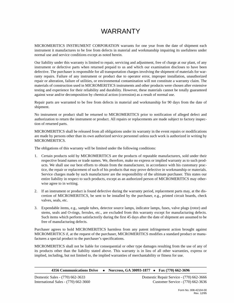
WARRANTY
MICROMERITICS INSTRUMENT CORPORATION warrants for one year from the date of shipment eachinstrument it manufactures to be free from defects in material and workmanship impairing its usefulness undernormal use and service conditions except as noted herein.
Our liability under this warranty is limited to repair, servicing and adjustment, free of charge at our plant, of anyinstrument or defective parts when returned prepaid to us and which our examination discloses to have beendefective. The purchaser is responsible for all transportation charges involving the shipment of materials for war-ranty repairs. Failure of any instrument or product due to operator error, improper installation, unauthorizedrepair or alteration, failure of utilities, or environmental contamination will not constitute a warranty claim. Thematerials of construction used in MICROMERITICS instruments and other products were chosen after extensivetesting and experience for their reliability and durability. However, these materials cannot be totally guaranteedagainst wear and/or decomposition by chemical action (corrosion) as a result of normal use.
Repair parts are warranted to be free from defects in material and workmanship for 90 days from the date ofshipment.
No instrument or product shall be returned to MICROMERITICS prior to notification of alleged defect andauthorization to return the instrument or product. All repairs or replacements are made subject to factory inspec-tion of returned parts.
MICROMERITICS shall be released from all obligations under its warranty in the event repairs or modificationsare made by persons other than its own authorized service personnel unless such work is authorized in writing byMICROMERITICS.
The obligations of this warranty will be limited under the following conditions:
1. Certain products sold by MICROMERITICS are the products of reputable manufacturers, sold under theirrespective brand names or trade names. We, therefore, make no express or implied warranty as to such prod-ucts. We shall use our best efforts to obtain from the manufacturer, in accordance with his customary prac-tice, the repair or replacement of such of his products that may prove defective in workmanship or materials.Service charges made by such manufacturer are the responsibility of the ultimate purchaser. This states ourentire liability in respect to such products, except as an authorized person of MICROMERITICS may other-wise agree to in writing.
2. If an instrument or product is found defective during the warranty period, replacement parts may, at the dis-cretion of MICROMERITICS, be sent to be installed by the purchaser, e.g., printed circuit boards, checkvalves, seals, etc.
3. Expendable items, e.g., sample tubes, detector source lamps, indicator lamps, fuses, valve plugs (rotor) andstems, seals and O-rings, ferrules, etc., are excluded from this warranty except for manufacturing defects.Such items which perform satisfactorily during the first 45 days after the date of shipment are assumed to befree of manufacturing defects.
Purchaser agrees to hold MICROMERITICS harmless from any patent infringement action brought againstMICROMERITICS if, at the request of the purchaser, MICROMERITICS modifies a standard product or manu-factures a special product to the purchaser’s specifications.
MICROMERITICS shall not be liable for consequential or other type damages resulting from the use of any ofits products other than the liability stated above. This warranty is in lieu of all other warranties, express orimplied, including, but not limited to, the implied warranties of merchantability or fitness for use.
4356 Communications Drive Norcross, GA 30093-1877 Fax (770) 662-3696
Domestic Sales - (770) 662-3633 Domestic Repair Service - (770) 662-3666International Sales - (770) 662-3660 Customer Service - (770) 662-3636
Rev. 12/95

Organization of the Operator’s Manual ASAP 2020 Confirm
1. GENERAL INFORMATION
This manual provides a description of the ASAP 2020 analyzer and the menu options and functions available for the ASAP 2020 Confirm program. This manual covers operations for a Developer and an Analyst. A Developer is authorized to perform all functions listed on the menu bar. An Analyst is restricted to certain functions which are enabled; the functions not authorized for an Analyst are disabled.
Organization of the Operator’s Manual
This operator’s manual is organized so that all basic operating procedures are located in Chapter 3. Chapters 4, 5, 6, and 7 contain detailed information on the dialogs used while performing these procedures. Refer to these chapters if you need clarification on a procedure. Many of the procedures and dialogs also are accessible through online help.
The ASAP 2020 Confirm operator’s manual is divided as follows:
Chapter 1 General Information.Provides a general description of the ASAP 2020 system as well as its specifications.
Chapter 2 USER INTERFACEProvides basic instrument and software interface.
Chapter 3 OPERATIONAL PROCEDURESProvides step-by-step instructions for operating the ASAP 2020.
Chapter 4 FILE MENU Provides a description of the commands on the File menu.
Chapter 5 UNIT MENUProvides a description of the commands on the Unit menu.
Chapter 6 REPORTS MENUProvides a description of the commands on the Reports menu and samples of reports.
Chapter 7 OPTIONS MENUProvides a description of the commands on the Options menu.
Chapter 8 TROUBLESHOOTING AND MAINTENANCE Provides instructions for troubleshooting hardware problems and for performing routine maintenance procedures.
May 06 1-1
ASAP 2020 Confirm Organization of the Operator’s Manual
Conventions
This document uses the symbols shown below to identify notes of importance, cautions, and warnings.
Chapter 9 ORDERING INFORMATIONProvides part numbers and descriptions of the ASAP 2020 System components and accessories.
Appendix A FORMSContains a form to assist you in determining the sample mass.
Appendix B ERROR MESSAGES Lists the error messages that may be displayed by the software/hardware; includes a cause and action for each.
Appendix C CALCULATIONSContains the calculations used by the system to produce reports.
Appendix D TESTING FOR LEAKS Describes the procedure for testing each valve for leaks.
Appendix E CALCULATING FREE-SPACE VALUES FOR MICROPORE ANALYSES Provides instructions for obtaining free-space values to use in micropore analyses.
Appendix F DFT MODELSProvides information on the models used with the DFT reports.
Notes contain a tip or important information pertinent to the subject matter.
Cautions contain information to help you prevent actions which could damage the instrument.
Warnings contain information to help you prevent actions which could cause personal injury.
1-2 May 06
Equipment Description ASAP 2020 Confirm
Equipment Description
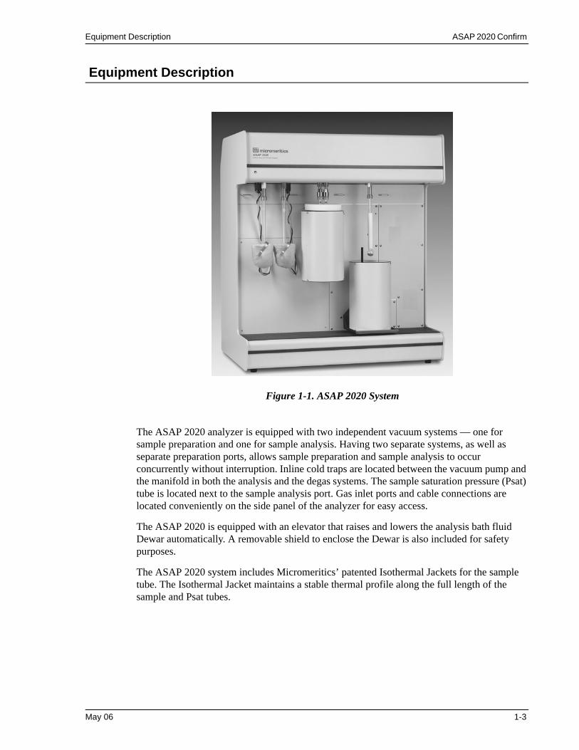
Figure 1-1. ASAP 2020 System
The ASAP 2020 analyzer is equipped with two independent vacuum systems — one for sample preparation and one for sample analysis. Having two separate systems, as well as separate preparation ports, allows sample preparation and sample analysis to occur concurrently without interruption. Inline cold traps are located between the vacuum pump and the manifold in both the analysis and the degas systems. The sample saturation pressure (Psat) tube is located next to the sample analysis port. Gas inlet ports and cable connections are located conveniently on the side panel of the analyzer for easy access.
The ASAP 2020 is equipped with an elevator that raises and lowers the analysis bath fluid Dewar automatically. A removable shield to enclose the Dewar is also included for safety purposes.
The ASAP 2020 system includes Micromeritics’ patented Isothermal Jackets for the sample tube. The Isothermal Jacket maintains a stable thermal profile along the full length of the sample and Psat tubes.
May 06 1-3
ASAP 2020 Confirm Equipment Description
Gas Requirements
Compressed gases are required for analyses performed by the ASAP 2020 analyzer. Gas bottles or an outlet from a central source should be located near the analyzer. Appropriate two-stage regulators which have been leak-checked and specially cleaned are required. Pressure relief valves should be set to no more than 30 psig (200 kPag). Gas regulators are available from Micromeritics; refer to Chapter 9, page 9-1 for ordering information.
Analysis Program
The ASAP 2020 Confirm software is designed to operate in a Windows 2000 or Windows XP Professional environment. The Windows environment provides a user-friendly interface for performing analyses and generating reports.
The ASAP 2020 Confirm software monitors and controls the analyzer. It enables you to perform automatic analyses with just a few key strokes, and collects and reports analysis data. You can choose from a variety of reports, which can be printed automatically after an analysis or stored and printed later.
Report System
The ASAP 2020 Confirm software includes a report system which allows you to manipulate and customize reports. You can zoom in on portions of the graphs or shift the axes to examine fine details. Scalable graphs can be copied to the clipboard and pasted into other applications. Reports can be customized with your choice of fonts and a company logo added to the report header for an impressive presentation. Refer to Chapter 6, page for the options available for reports.
If you are new to Windows, you should learn some basic Windows skills, such as using the mouse and choosing commands. Brief instructions are provided in Chapter 3. For more specific instructions, refer to the Windows documentation or its online help system.
1-4 May 06
Online Manual ASAP 2020 Confirm
Online Manual
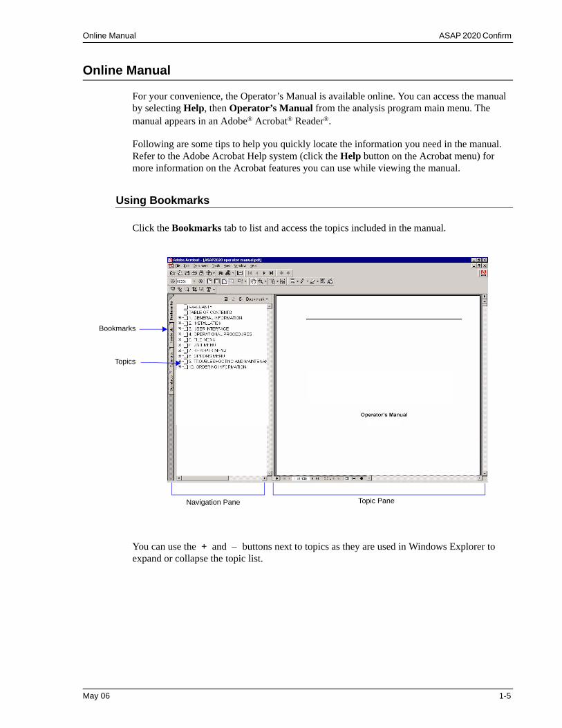
For your convenience, the Operator’s Manual is available online. You can access the manual by selecting Help, then Operator’s Manual from the analysis program main menu. The manual appears in an Adobe® Acrobat® Reader®.
Following are some tips to help you quickly locate the information you need in the manual. Refer to the Adobe Acrobat Help system (click the Help button on the Acrobat menu) for more information on the Acrobat features you can use while viewing the manual.
Using Bookmarks
Click the Bookmarks tab to list and access the topics included in the manual.
You can use the + and − buttons next to topics as they are used in Windows Explorer to expand or collapse the topic list.
Navigation Pane Topic Pane
Bookmarks
Topics
May 06 1-5
ASAP 2020 Confirm Online Manual
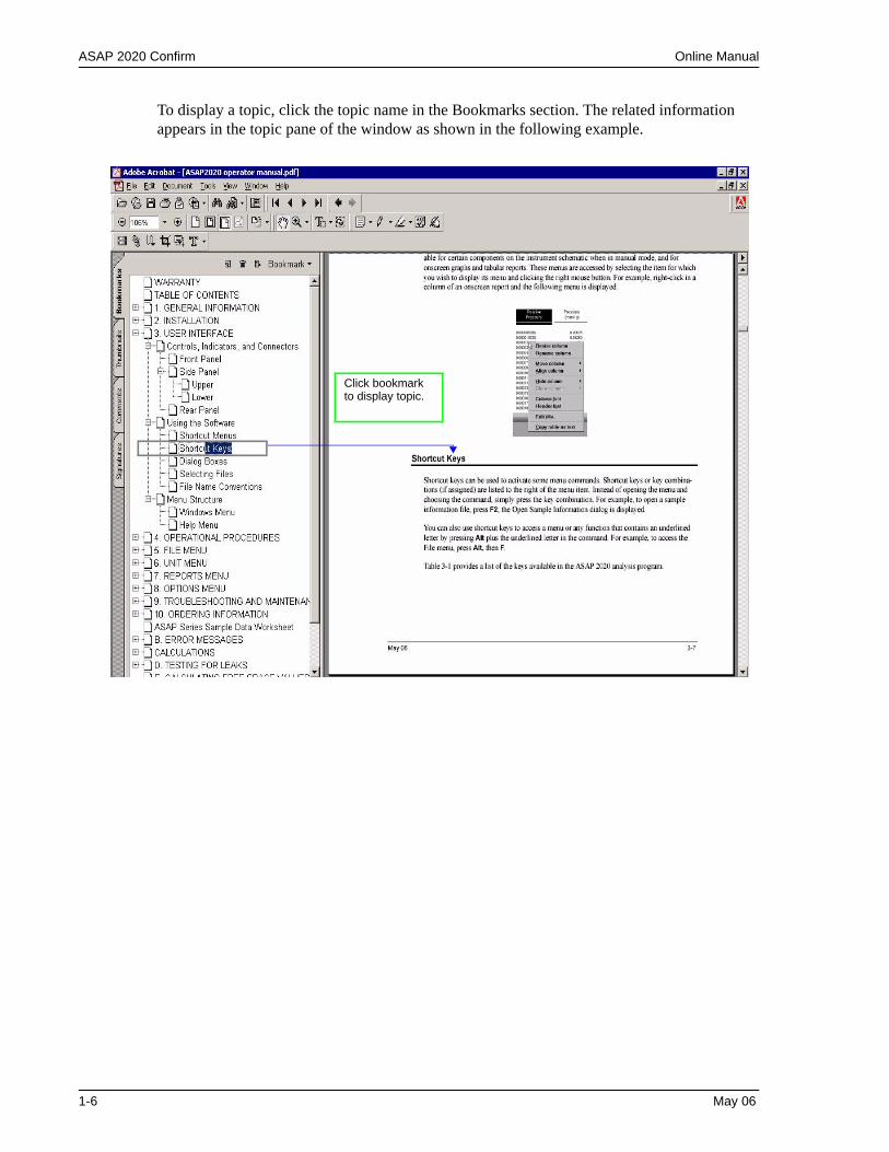
To display a topic, click the topic name in the Bookmarks section. The related information appears in the topic pane of the window as shown in the following example.
Click bookmarkto display topic.
1-6 May 06
Online Manual ASAP 2020 Confirm
Using the Table of Contents, Index, and other Links
Links provide direct access to selected information. All links appear in blue type. Links are contained in:
• the table of contents• index entries• cross-references within the manual
Table of Contents
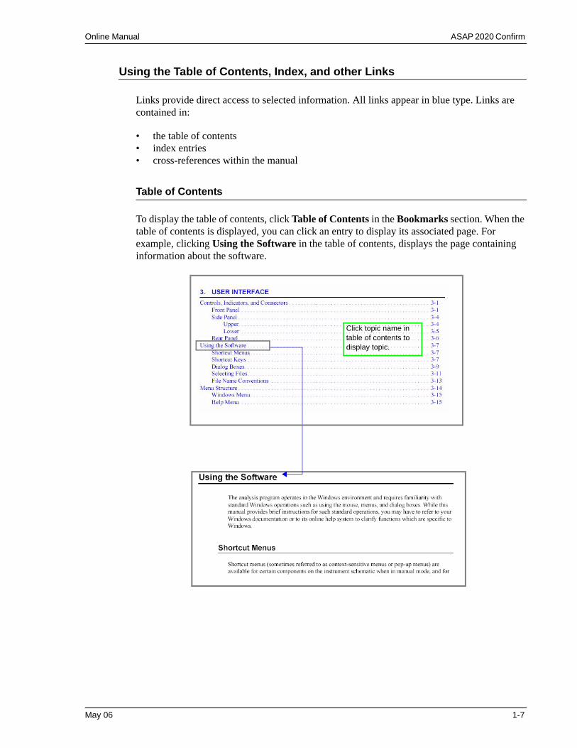
To display the table of contents, click Table of Contents in the Bookmarks section. When the table of contents is displayed, you can click an entry to display its associated page. For example, clicking Using the Software in the table of contents, displays the page containing information about the software.
Click topic name in table of contents to display topic.
May 06 1-7
ASAP 2020 Confirm Online Manual
Index
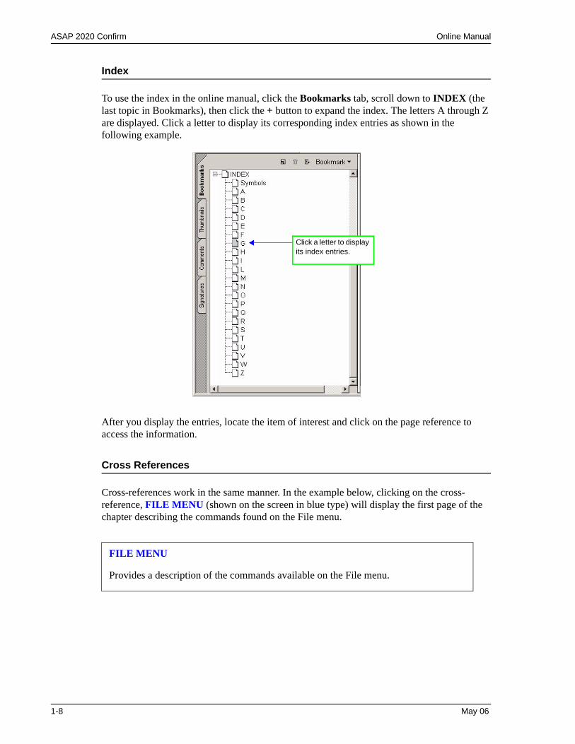
To use the index in the online manual, click the Bookmarks tab, scroll down to INDEX (the last topic in Bookmarks), then click the + button to expand the index. The letters A through Z are displayed. Click a letter to display its corresponding index entries as shown in the following example.
After you display the entries, locate the item of interest and click on the page reference to access the information.
Cross References
Cross-references work in the same manner. In the example below, clicking on the cross-reference, FILE MENU (shown on the screen in blue type) will display the first page of the chapter describing the commands found on the File menu.
FILE MENU
Provides a description of the commands available on the File menu.
Click a letter to display its index entries.
1-8 May 06
Online Manual ASAP 2020 Confirm
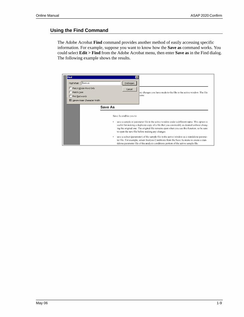
Using the Find Command
The Adobe Acrobat Find command provides another method of easily accessing specific information. For example, suppose you want to know how the Save as command works. You could select Edit > Find from the Adobe Acrobat menu, then enter Save as in the Find dialog. The following example shows the results.
May 06 1-9
ASAP 2020 Confirm Online Manual
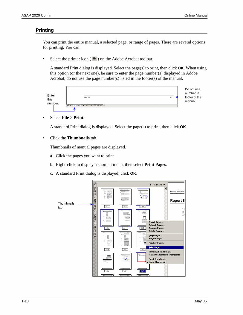
Printing
You can print the entire manual, a selected page, or range of pages. There are several options for printing. You can:
• Select the printer icon ( ) on the Adobe Acrobat toolbar.
A standard Print dialog is displayed. Select the page(s) to print, then click OK. When using this option (or the next one), be sure to enter the page number(s) displayed in Adobe Acrobat; do not use the page number(s) listed in the footer(s) of the manual.
• Select File > Print.
A standard Print dialog is displayed. Select the page(s) to print, then click OK.
• Click the Thumbnails tab.
Thumbnails of manual pages are displayed.
a. Click the pages you want to print.
b. Right-click to display a shortcut menu, then select Print Pages.
c. A standard Print dialog is displayed; click OK.
Enter this number.
Do not use number in footer of the manual.
Thumbnails tab
1-10 May 06
Internet Access ASAP 2020 Confirm
Internet Access
Visit www.micromeritics.com to learn more about Micromeritics, our products, and applica-tions. Our site is user-friendly, easy to navigate, and informative. Its content is summarized below.
Be sure to browse our site to see the many ways in which we can assist you.
About Micromeritics A brief history of Micromeritics, office locations, awards/cer-tifications, career opportunities, and a virtual tour of its headquarters
Products Product information and printable brochures
Applications Application Notes, Product Bulletins, Tech Tips, Technical Articles/papers, and important application links
Online Catalog Catalog of instruments and accessories, allowing you to place your order online
News and Press Press releases, Events calendar, microReports, and latest Micromeritics news updates
Lab Service Provides laboratory tips and access to the Micromeritics Ana-lytical Services web site
Customer Support Customer support contacts, product registration, instrument training information, Material Safety Data Sheets, and account registration
Grant Program Details of the Grant Program established for non-profit orga-nizations and universities
Contact Us Contact information, office locations, maps and driving direc-tions to the Micromeritics facility, and registration for the microReport newsletter
May 06 1-11
ASAP 2020 Confirm Specifications
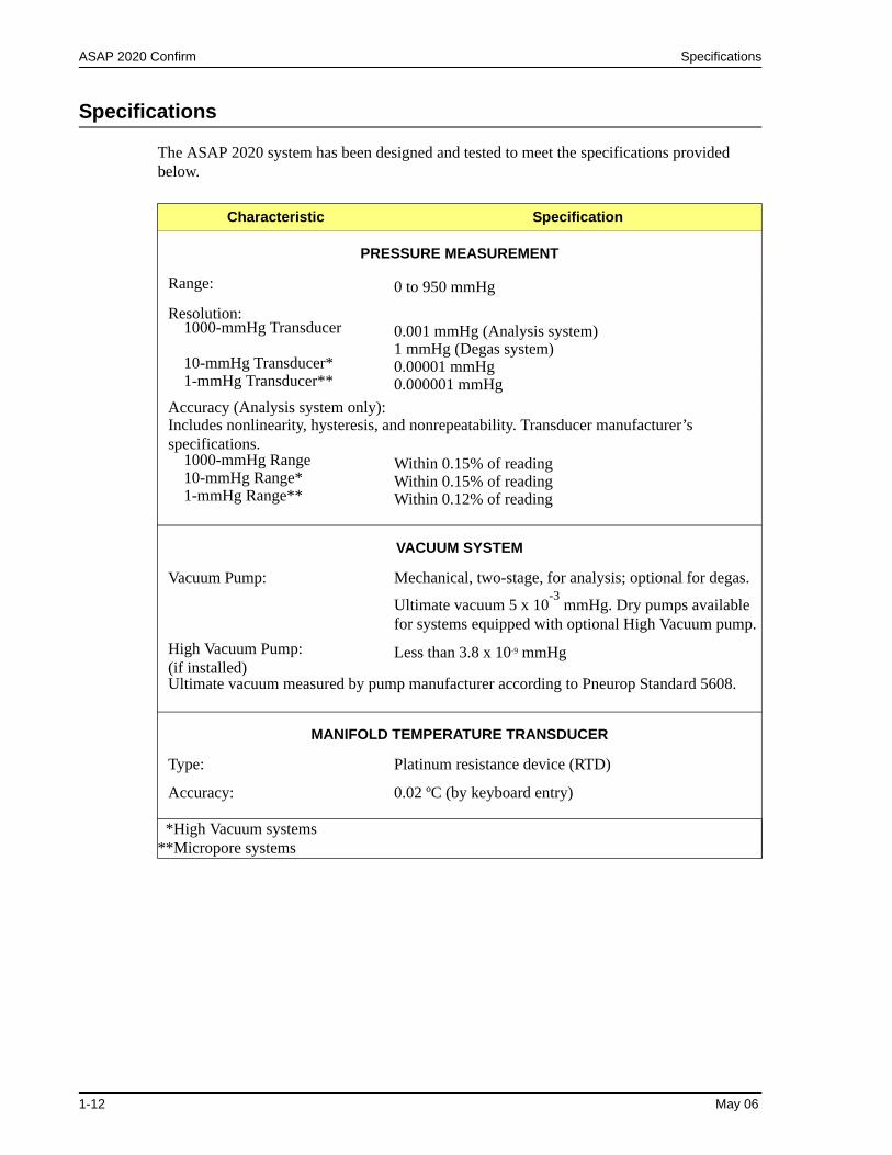
Specifications
The ASAP 2020 system has been designed and tested to meet the specifications provided below.
Characteristic Specification
PRESSURE MEASUREMENT
Range: 0 to 950 mmHg
Resolution:1000-mmHg Transducer 0.001 mmHg (Analysis system)
1 mmHg (Degas system)10-mmHg Transducer* 0.00001 mmHg1-mmHg Transducer** 0.000001 mmHg
Accuracy (Analysis system only):Includes nonlinearity, hysteresis, and nonrepeatability. Transducer manufacturer’s specifications.
1000-mmHg Range Within 0.15% of reading10-mmHg Range* Within 0.15% of reading1-mmHg Range** Within 0.12% of reading
VACUUM SYSTEM
Vacuum Pump: Mechanical, two-stage, for analysis; optional for degas.
Ultimate vacuum 5 x 10⁻³ mmHg. Dry pumps available for systems equipped with optional High Vacuum pump.
High Vacuum Pump:(if installed)
Less than 3.8 x 10⁻⁹ mmHg
Ultimate vacuum measured by pump manufacturer according to Pneurop Standard 5608.
MANIFOLD TEMPERATURE TRANSDUCER
Type: Platinum resistance device (RTD)
Accuracy: 0.02 ºC (by keyboard entry)
*High Vacuum systems**Micropore systems
1-12 May 06
Specifications ASAP 2020 Confirm
Characteristic Specification
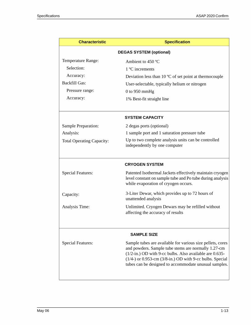
DEGAS SYSTEM (optional)
Temperature Range: Ambient to 450 ºCSelection: 1 ºC incrementsAccuracy: Deviation less than 10 ºC of set point at thermocouple
Backfill Gas: User-selectable, typically helium or nitrogenPressure range: 0 to 950 mmHgAccuracy: 1% Best-fit straight line
SYSTEM CAPACITY
Sample Preparation: 2 degas ports (optional)Analysis: 1 sample port and 1 saturation pressure tube
Total Operating Capacity: Up to two complete analysis units can be controlled independently by one computer
CRYOGEN SYSTEM
Special Features: Patented Isothermal Jackets effectively maintain cryogen level constant on sample tube and Po tube during analysis while evaporation of cryogen occurs.
Capacity: 3-Liter Dewar, which provides up to 72 hours of unattended analysis
Analysis Time: Unlimited. Cryogen Dewars may be refilled without affecting the accuracy of results
SAMPLE SIZE
Special Features: Sample tubes are available for various size pellets, cores and powders. Sample tube stems are normally 1.27-cm (1/2-in.) OD with 9-cc bulbs. Also available are 0.635- (1/4-) or 0.953-cm (3/8-in.) OD with 9-cc bulbs. Special tubes can be designed to accommodate unusual samples.
May 06 1-13
ASAP 2020 Confirm Specifications
Characteristic Specification
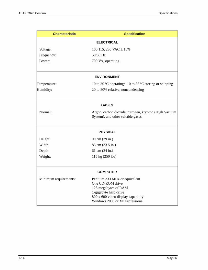
ELECTRICAL
Voltage: 100,115, 230 VAC ± 10%Frequency: 50/60 HzPower: 700 VA, operating
ENVIRONMENT
Temperature: 10 to 30 ºC operating; -10 to 55 ºC storing or shippingHumidity: 20 to 80% relative, noncondensing
GASES
Normal: Argon, carbon dioxide, nitrogen, krypton (High Vacuum System), and other suitable gases
PHYSICAL
Height: 99 cm (39 in.)Width: 85 cm (33.5 in.)Depth: 61 cm (24 in.)Weight: 115 kg (250 lbs)
COMPUTER
Minimum requirements: Pentium 333 MHz or equivalentOne CD-ROM drive128 megabytes of RAM1-gigabyte hard drive800 x 600 video display capabilityWindows 2000 or XP Professional
1-14 May 06
Controls, Indicators, and Connectors ASAP 2020 Confirm
2. USER INTERFACE
The ASAP 2020 Confirm software is accessed by three different levels of users:
• Administrator: installs and maintains software and updates, establishes user accounts and rights (the Administrator responsibilities are covered in a separate manual).
• Developer: has access to all functions of the software. A Developer’s primary function is to create templates for an Analyst.
• Analyst: creates sample files from predefined templates; some fields, such as the Mass field, are enabled and can be edited. An Analyst is also allowed to perform other tasks as designated throughout this manual. Tasks not allowed are disabled.
This manual is written for the Developer and Analyst levels of the ASAP 2020 Confirm software. Functions for the Administrator level are covered in the Administrator Utility User’s Guide.
This chapter contains information to familiarize you with the hardware and software of the ASAP 2020 system. It is recommended that you read this chapter before attempting to operate the ASAP 2020 system.
Controls, Indicators, and Connectors
This section contains a description of the controls, indicators, and connectors located on the front, side, and rear panels of the ASAP 2020 system.
May 06 2-1
ASAP 2020 Confirm Controls, Indicators, and Connectors
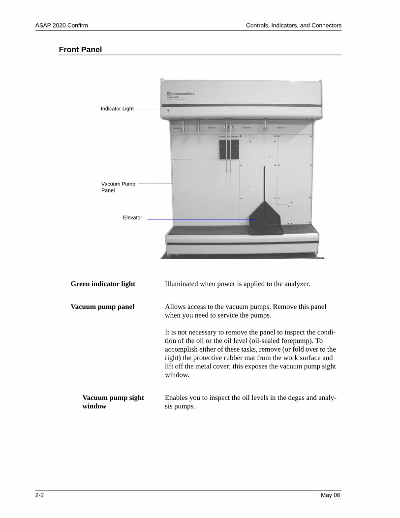
Front Panel
Green indicator light Illuminated when power is applied to the analyzer.
Vacuum pump panel Allows access to the vacuum pumps. Remove this panel when you need to service the pumps.
It is not necessary to remove the panel to inspect the condi-tion of the oil or the oil level (oil-sealed forepump). To accomplish either of these tasks, remove (or fold over to the right) the protective rubber mat from the work surface and lift off the metal cover; this exposes the vacuum pump sight window.
Vacuum pump sightwindow
Enables you to inspect the oil levels in the degas and analy-sis pumps.
Indicator Light
Vacuum Pump Panel
Elevator
2-2 May 06
Controls, Indicators, and Connectors ASAP 2020 Confirm
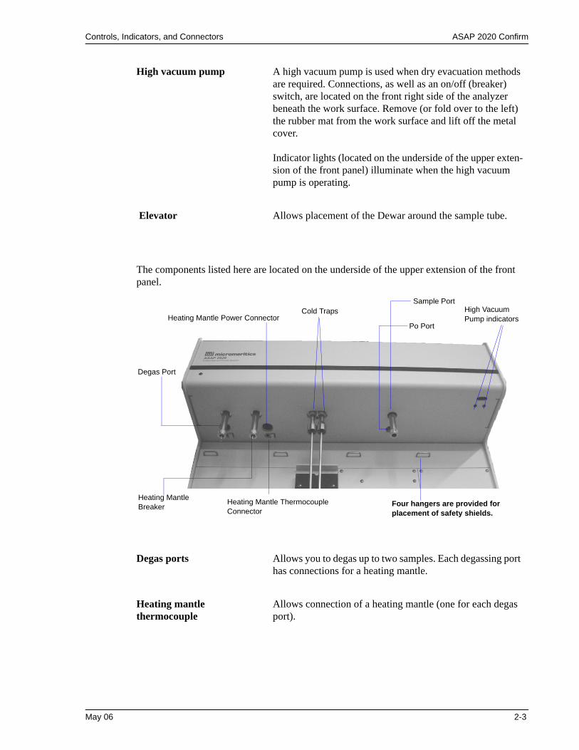
The components listed here are located on the underside of the upper extension of the front panel.
High vacuum pump A high vacuum pump is used when dry evacuation methods are required. Connections, as well as an on/off (breaker) switch, are located on the front right side of the analyzer beneath the work surface. Remove (or fold over to the left) the rubber mat from the work surface and lift off the metal cover.
Indicator lights (located on the underside of the upper exten-sion of the front panel) illuminate when the high vacuum pump is operating.
Elevator Allows placement of the Dewar around the sample tube.
Degas ports Allows you to degas up to two samples. Each degassing port has connections for a heating mantle.
Heating mantle thermocouple
Allows connection of a heating mantle (one for each degas port).
Po PortHeating Mantle Power Connector
Degas Port
Heating Mantle Thermocouple Connector
Sample PortHigh Vacuum Pump indicators
Heating Mantle Breaker
Cold Traps
Four hangers are provided for placement of safety shields.
May 06 2-3
ASAP 2020 Confirm Controls, Indicators, and Connectors
Heating mantle power connector
Allows connection of the heating mantle power cord (one for each heating mantle).
Heating mantlebreaker
Protects the circuitry for the heating mantle in the event of a failure (one for each heating mantle). If the circuit breaker trips (pops out), call your Micromeritics service representa-tive.
Cold Traps Two cold traps are provided; one for degassing and one for analysis.
High vacuum pump indicators
Illuminate when the high vacuum pump(s) is(are) operating at normal speed. The left indicator is for degas operations and the right one for analysis.
Sample port For installing the sample tube containing the material you wish to analyze.
Po port For installing a Po (saturation pressure) tube when perform-ing physisorption analyses.
2-4 May 06
Controls, Indicators, and Connectors ASAP 2020 Confirm
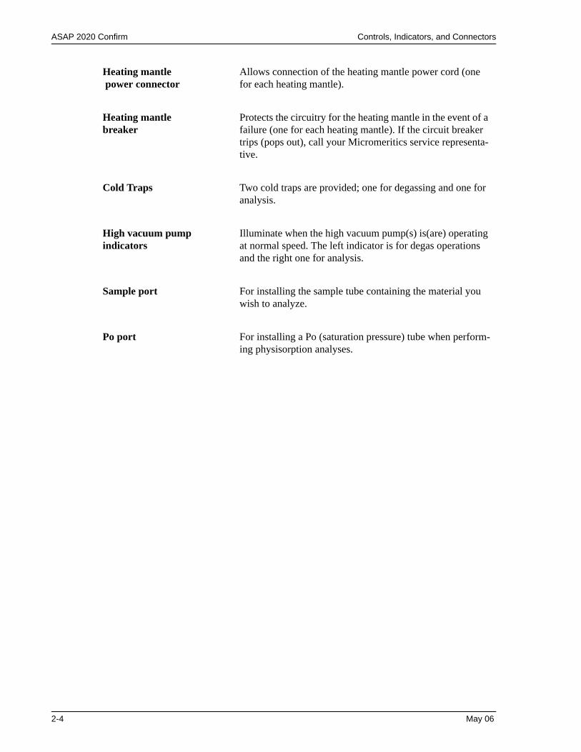
Side Panel
Upper
Gas inlet ports Used to connect gas supplies to the analyzer.
Vapor gas port For attaching the water vapor option, or connecting a vapor gas. Refer to Chapter 9, page 9-1 for ordering information on the water vapor option.
Degas port Allows connection of a gas to use for degassing the sample.
Helium port Allows connection of helium to use for measuring the free space.
Gas Inlet Ports
Chemisorption Ports (available if upgraded to Chemisorption capability)
Degas Port
Helium Port
Vapor Gas Port
May 06 2-5
ASAP 2020 Confirm Controls, Indicators, and Connectors
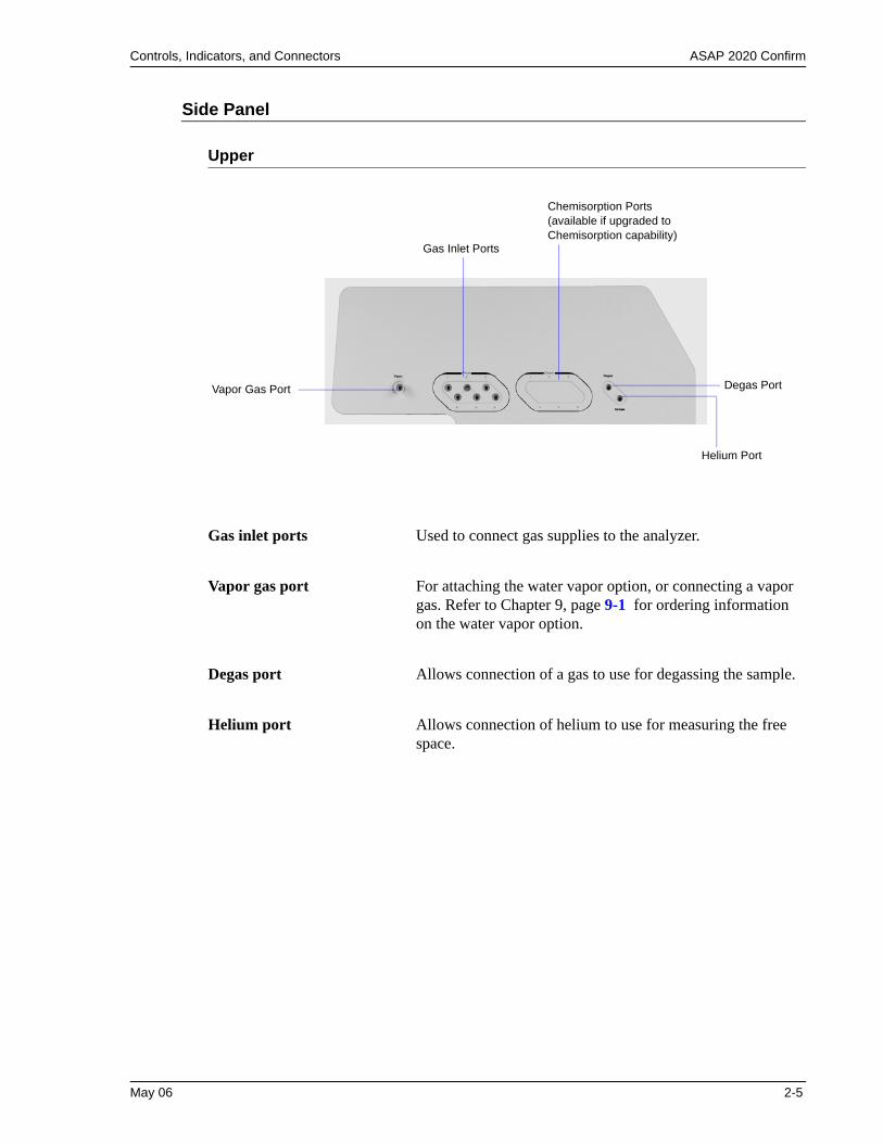
Lower
On/Off switch For turning the analyzer on and off. This switch also serves as the main breaker for the analyzer; it switches off auto-matically in the event of an electrical fault.
Power connector For connecting the analyzer to the electrical supply.
RS232 port For connecting the analyzer to a computer.
Valve circuit breaker Protects the circuitry for the valves in the event of a failure. If the circuit breaker trips (pops out) and continues to trip after being reset, call your Micromeritics service representa-tive.
Voltage selector switch For setting the analyzer to the correct incoming AC line voltage.
On/Off Switch
Power Connector
Voltage Selector Switch
Valve Circuit Breaker
RS 232 Port
2-6 May 06
Controls, Indicators, and Connectors ASAP 2020 Confirm
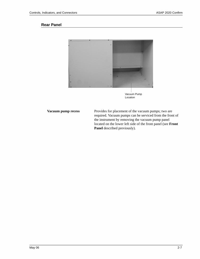
Rear Panel
Vacuum pump recess Provides for placement of the vacuum pumps; two are required. Vacuum pumps can be serviced from the front of the instrument by removing the vacuum pump panel located on the lower left side of the front panel (see Front Panel described previously).
Vacuum Pump Location
May 06 2-7
ASAP 2020 Confirm Using the Software
Using the Software
The ASAP 2020 Confirm Program operates in the Windows environment and requires familiarity with standard Windows operations such as using the mouse, menus, and dialog boxes. While this manual provides brief instructions for such standard operations, you may have to refer to your Windows documentation or to its online help system to clarify functions which are specific to Windows.
Logging In
Each user — Administrator, Developer, or Analyst — is required to enter a user name and password when opening the application. Initially, the Administrator establishes passwords for the Developer and Analyst(s) when the software is installed. These passwords are temporary and are used for initial log-in; at that time, each user is prompted to specify a password that only he/she knows.
Your password must consist of at least six characters and expires after a specified time (designated by the Administrator). You will be locked out of the application if you fail to enter the correct password after three (default) tries. This number can be changed by your Administrator. The Administrator is also required to unlock the application in the event it becomes locked after failure to enter the correct password.
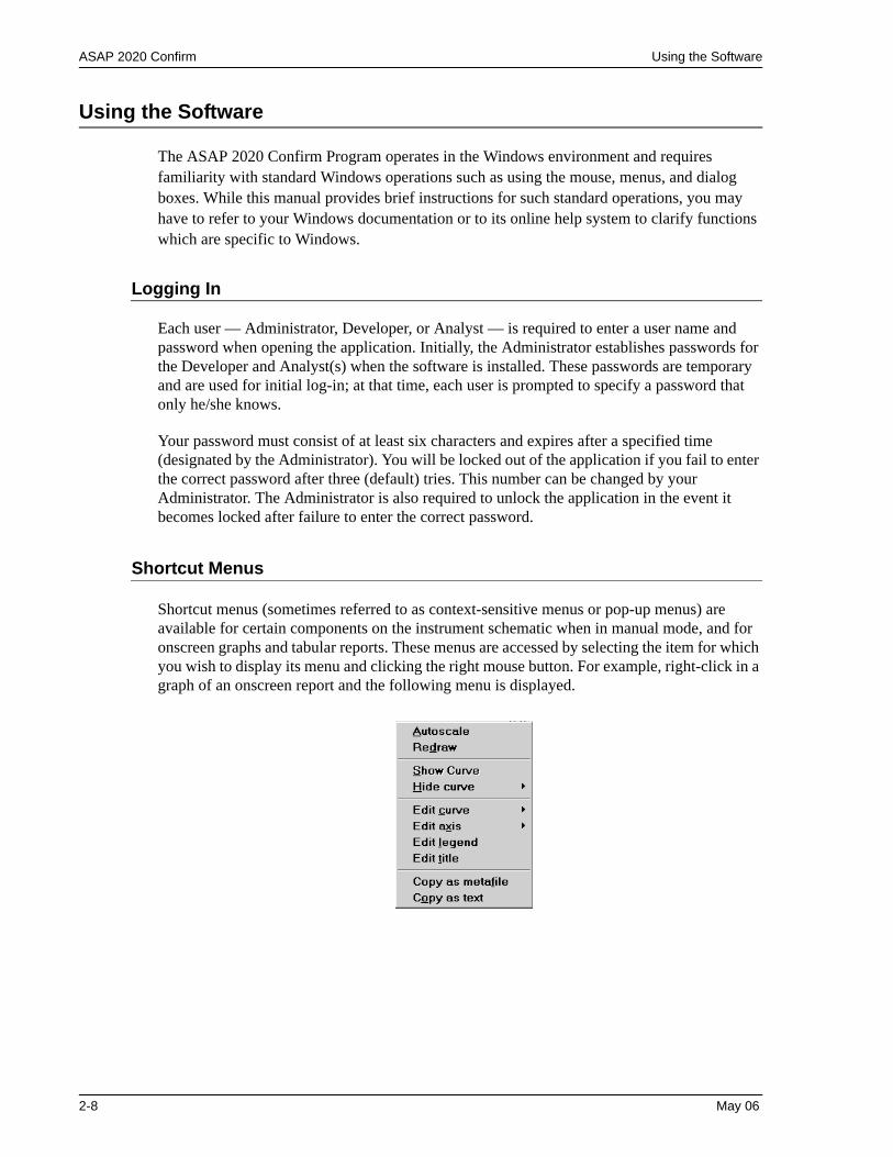
Shortcut Menus
Shortcut menus (sometimes referred to as context-sensitive menus or pop-up menus) are available for certain components on the instrument schematic when in manual mode, and for onscreen graphs and tabular reports. These menus are accessed by selecting the item for which you wish to display its menu and clicking the right mouse button. For example, right-click in a graph of an onscreen report and the following menu is displayed.
2-8 May 06
Using the Software ASAP 2020 Confirm
Shortcut Keys
Shortcut keys can be used to activate some menu commands. Shortcut keys or key combinations (if assigned) are listed to the right of the menu item. Instead of opening the menu and choosing the command, simply press the key combination. For example, to open a sample information file, press F2; the Open Sample Information dialog is displayed.
You can also use shortcut keys to access a menu or any function that contains an underlined letter by pressing Alt plus the underlined letter in the command. For example, to access the File menu, press Alt, then F.
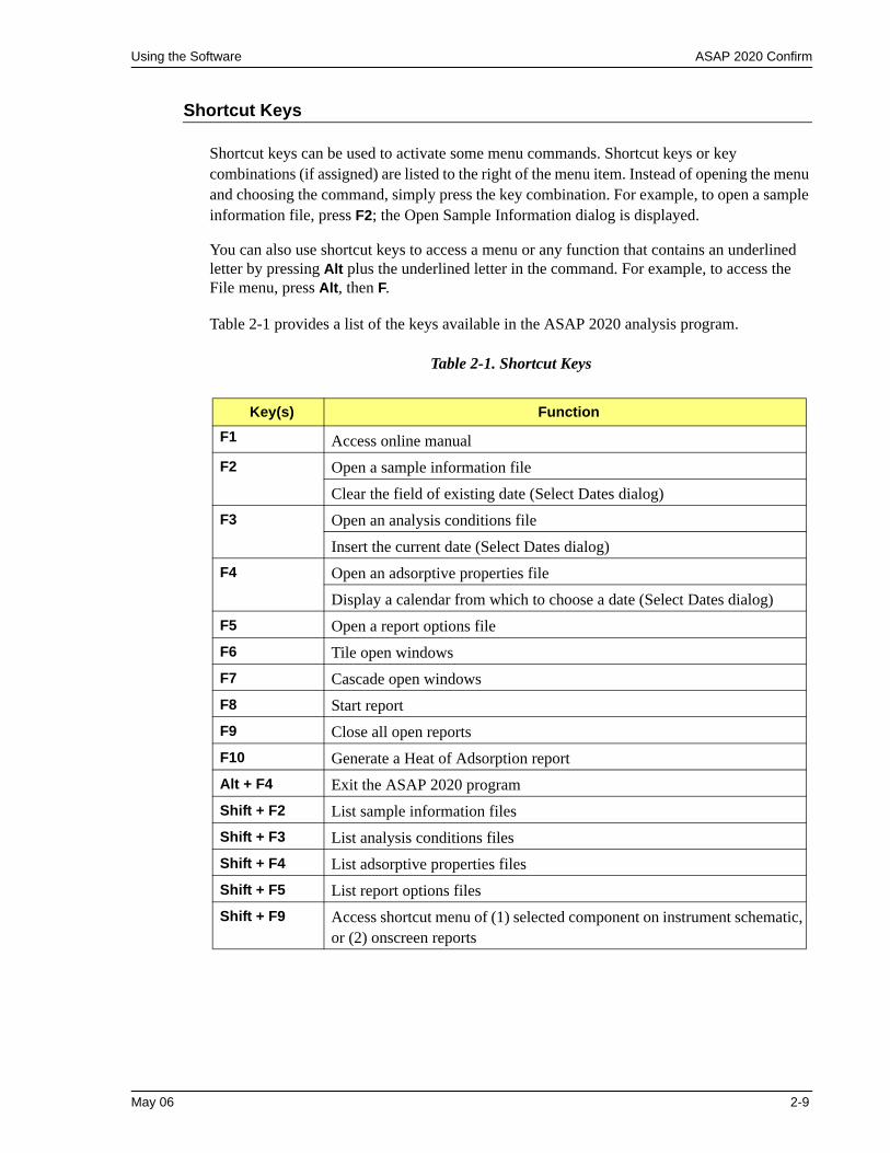
Table 2-1 provides a list of the keys available in the ASAP 2020 analysis program.
Table 2-1. Shortcut Keys
Key(s) FunctionF1 Access online manualF2 Open a sample information file
Clear the field of existing date (Select Dates dialog)F3 Open an analysis conditions file
Insert the current date (Select Dates dialog)F4 Open an adsorptive properties file
Display a calendar from which to choose a date (Select Dates dialog)F5 Open a report options fileF6 Tile open windowsF7 Cascade open windowsF8 Start reportF9 Close all open reportsF10 Generate a Heat of Adsorption reportAlt + F4 Exit the ASAP 2020 programShift + F2 List sample information filesShift + F3 List analysis conditions filesShift + F4 List adsorptive properties filesShift + F5 List report options filesShift + F9 Access shortcut menu of (1) selected component on instrument schematic,
or (2) onscreen reports
May 06 2-9
ASAP 2020 Confirm Using the Software
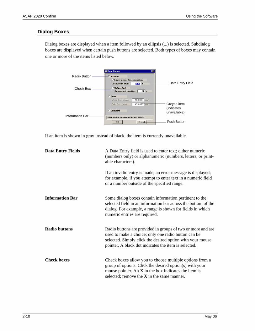
Dialog Boxes
Dialog boxes are displayed when a item followed by an ellipsis (...) is selected. Subdialog boxes are displayed when certain push buttons are selected. Both types of boxes may contain one or more of the items listed below.
If an item is shown in gray instead of black, the item is currently unavailable.
Data Entry Fields A Data Entry field is used to enter text; either numeric (numbers only) or alphanumeric (numbers, letters, or print-able characters).
If an invalid entry is made, an error message is displayed; for example, if you attempt to enter text in a numeric field or a number outside of the specified range.
Information Bar Some dialog boxes contain information pertinent to the selected field in an information bar across the bottom of the dialog. For example, a range is shown for fields in which numeric entries are required.
Radio buttons Radio buttons are provided in groups of two or more and are used to make a choice; only one radio button can be selected. Simply click the desired option with your mouse pointer. A black dot indicates the item is selected.
Check boxes Check boxes allow you to choose multiple options from a group of options. Click the desired option(s) with your mouse pointer. An X in the box indicates the item is selected; remove the X in the same manner.
Data Entry Field
Greyed item (indicates unavailable)
Push Button
Information Bar
Check Box
Radio Button
2-10 May 06
Using the Software ASAP 2020 Confirm
Push Buttons A push button is used to display a subdialog box in which to enter additional information about the subject matter, or to invoke an action.
For example, if you click Dates on the Open Sample Infor-mation dialog box, the Select Dates subdialog box is dis-played (explained in the next section). If you click Cancel on the Open Sample Information dialog box, you invoke the action of canceling and closing the dialog box.
Close Closes the active dialog box. If the dialog box contains unsaved changes, you will be prompted to save them before the dialog box closes.
Any information entered in subdialog boxes (refer to the next section of this chapter), is discarded also.
Save Saves the information entered in the current session; the dia-log box remains open.
Replace Allows you to replace the contents of the current file with those from an existing file. For example, if you are creating an analysis conditions file, you can save time by clicking and choosing the file containing the values you wish to use. These values are copied into the current file automatically And since the values are actually just copied into the file, you can edit them in any way you wish. The file from which they were copied remains intact and ready for the next use.
Cancel Discards everything you entered in the dialog box and any subdialog boxes, and closes the dialog box. A warning mes-sage is displayed before closing.
Drop-down list A drop-down list contains a list of options and is indicated by a down arrow to the right of the field. If there are more items than can fit in the box, a scroll bar is provided for nav-igating through the list.
May 06 2-11
ASAP 2020 Confirm Using the Software
Selecting Files
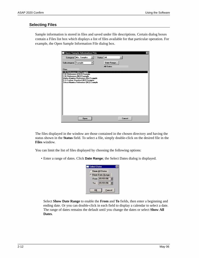
Sample information is stored in files and saved under file descriptions. Certain dialog boxes contain a Files list box which displays a list of files available for that particular operation. For example, the Open Sample Information File dialog box.
The files displayed in the window are those contained in the chosen directory and having the status shown in the Status field. To select a file, simply double-click on the desired file in the Files window.
You can limit the list of files displayed by choosing the following options:
• Enter a range of dates. Click Date Range; the Select Dates dialog is displayed.
Select Show Date Range to enable the From and To fields, then enter a beginning and ending date. Or you can double-click in each field to display a calendar to select a date. The range of dates remains the default until you change the dates or select Show All Dates.
2-12 May 06
Using the Software ASAP 2020 Confirm
For convenience, the following shortcut keys are available when the Select Dates dialog is displayed:
F2 Clears the dateF3 Inserts the current dateF4 Displays a calendar from which you may select a date
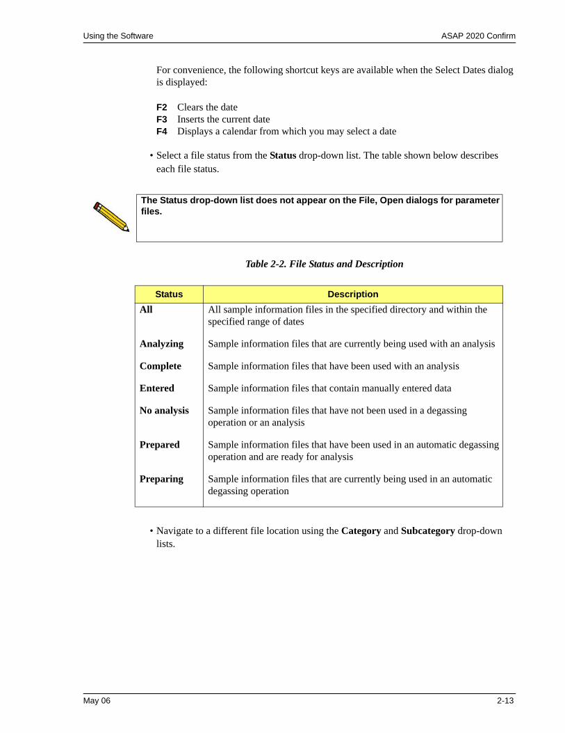
• Select a file status from the Status drop-down list. The table shown below describes each file status.
Table 2-2. File Status and Description
• Navigate to a different file location using the Category and Subcategory drop-down lists.
The Status drop-down list does not appear on the File, Open dialogs for parameter files.
Status DescriptionAll All sample information files in the specified directory and within the
specified range of dates
Analyzing Sample information files that are currently being used with an analysis
Complete Sample information files that have been used with an analysis
Entered Sample information files that contain manually entered data
No analysis Sample information files that have not been used in a degassing operation or an analysis
Prepared Sample information files that have been used in an automatic degassing operation and are ready for analysis
Preparing Sample information files that are currently being used in an automatic degassing operation
May 06 2-13
ASAP 2020 Confirm Menu Structure
Menu Structure
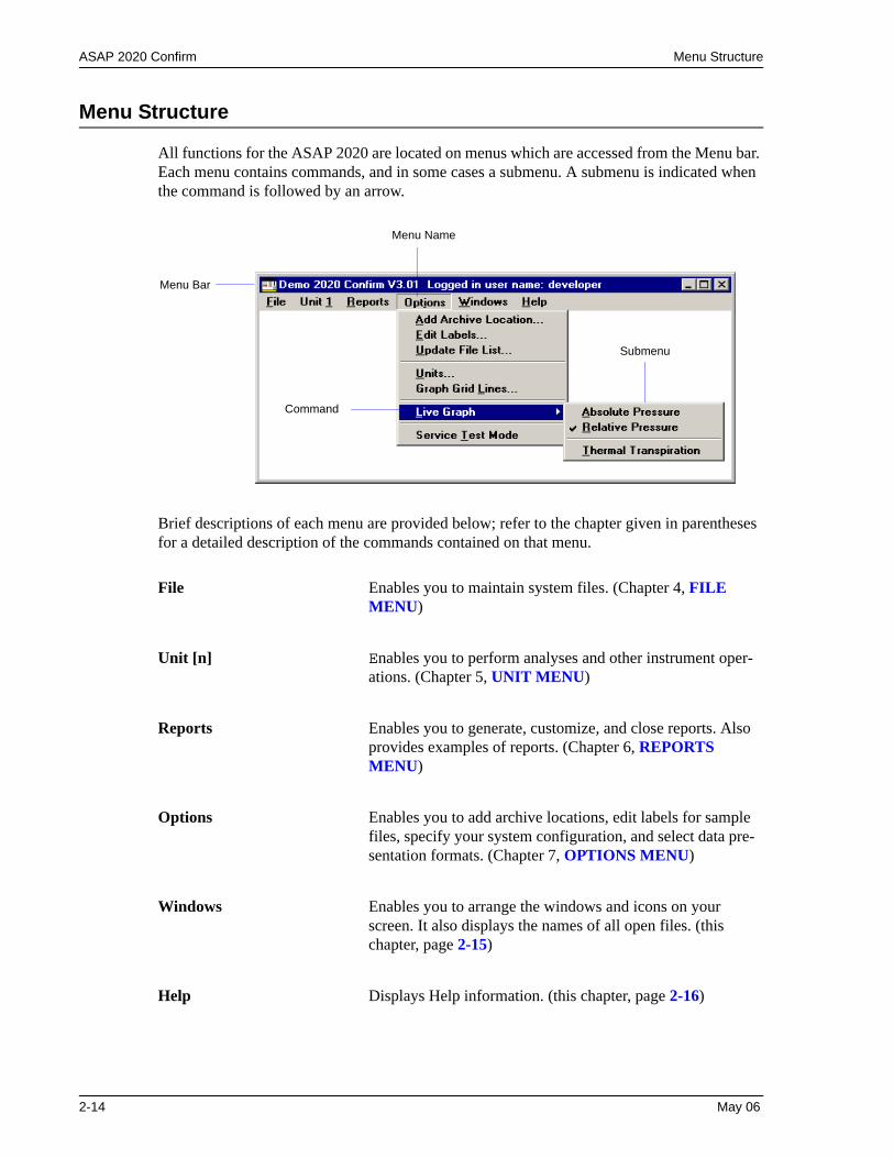
All functions for the ASAP 2020 are located on menus which are accessed from the Menu bar. Each menu contains commands, and in some cases a submenu. A submenu is indicated when the command is followed by an arrow.
Brief descriptions of each menu are provided below; refer to the chapter given in parentheses for a detailed description of the commands contained on that menu.
File Enables you to maintain system files. (Chapter 4, FILE MENU)
Unit [n] Enables you to perform analyses and other instrument oper-ations. (Chapter 5, UNIT MENU)
Reports Enables you to generate, customize, and close reports. Also provides examples of reports. (Chapter 6, REPORTS MENU)
Options Enables you to add archive locations, edit labels for sample files, specify your system configuration, and select data pre-sentation formats. (Chapter 7, OPTIONS MENU)
Windows Enables you to arrange the windows and icons on your screen. It also displays the names of all open files. (this chapter, page 2-15)
Help Displays Help information. (this chapter, page 2-16)
Menu Name
Command
Menu Bar
Submenu
2-14 May 06
Menu Structure ASAP 2020 Confirm
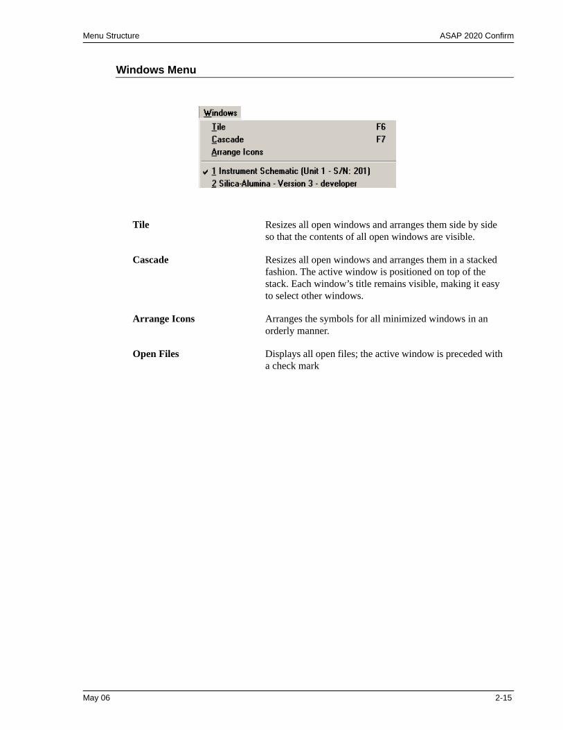
Windows Menu
Tile Resizes all open windows and arranges them side by side so that the contents of all open windows are visible.
Cascade Resizes all open windows and arranges them in a stacked fashion. The active window is positioned on top of the stack. Each window’s title remains visible, making it easy to select other windows.
Arrange Icons Arranges the symbols for all minimized windows in an orderly manner.
Open Files Displays all open files; the active window is preceded with a check mark
May 06 2-15
ASAP 2020 Confirm Menu Structure
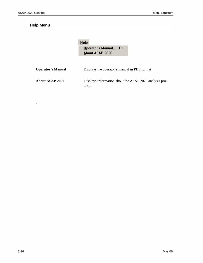
Help Menu
.
Operator’s Manual Displays the operator’s manual in PDF format
About ASAP 2020 Displays information about the ASAP 2020 analysis pro-gram
2-16 May 06
Creating File Templates ASAP 2020 Confirm
3. OPERATIONAL PROCEDURES
This chapter contains step-by-step procedures for operating the ASAP 2020 Confirm program. It does not provide detailed descriptions of the fields in the dialogs used to perform these procedures. Refer to Chapters 4 through 7 for field descriptions.
Some procedures cannot be performed by the Analyst; these procedures are marked accordingly.
Creating File Templates
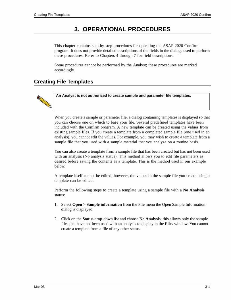
When you create a sample or parameter file, a dialog containing templates is displayed so that you can choose one on which to base your file. Several predefined templates have been included with the Confirm program. A new template can be created using the values from existing sample files. If you create a template from a completed sample file (one used in an analysis), you cannot edit the values. For example, you may wish to create a template from a sample file that you used with a sample material that you analyze on a routine basis.
You can also create a template from a sample file that has been created but has not been used with an analysis (No analysis status). This method allows you to edit file parameters as desired before saving the contents as a template. This is the method used in our example below.
A template itself cannot be edited; however, the values in the sample file you create using a template can be edited.
Perform the following steps to create a template using a sample file with a No Analysis status:
1. Select Open > Sample information from the File menu the Open Sample Information dialog is displayed.
2. Click on the Status drop-down list and choose No Analysis; this allows only the sample files that have not been used with an analysis to display in the Files window. You cannot create a template from a file of any other status.
An Analyst is not authorized to create sample and parameter file templates.
Mar 08 3-1
ASAP 2020 Confirm Creating File Templates
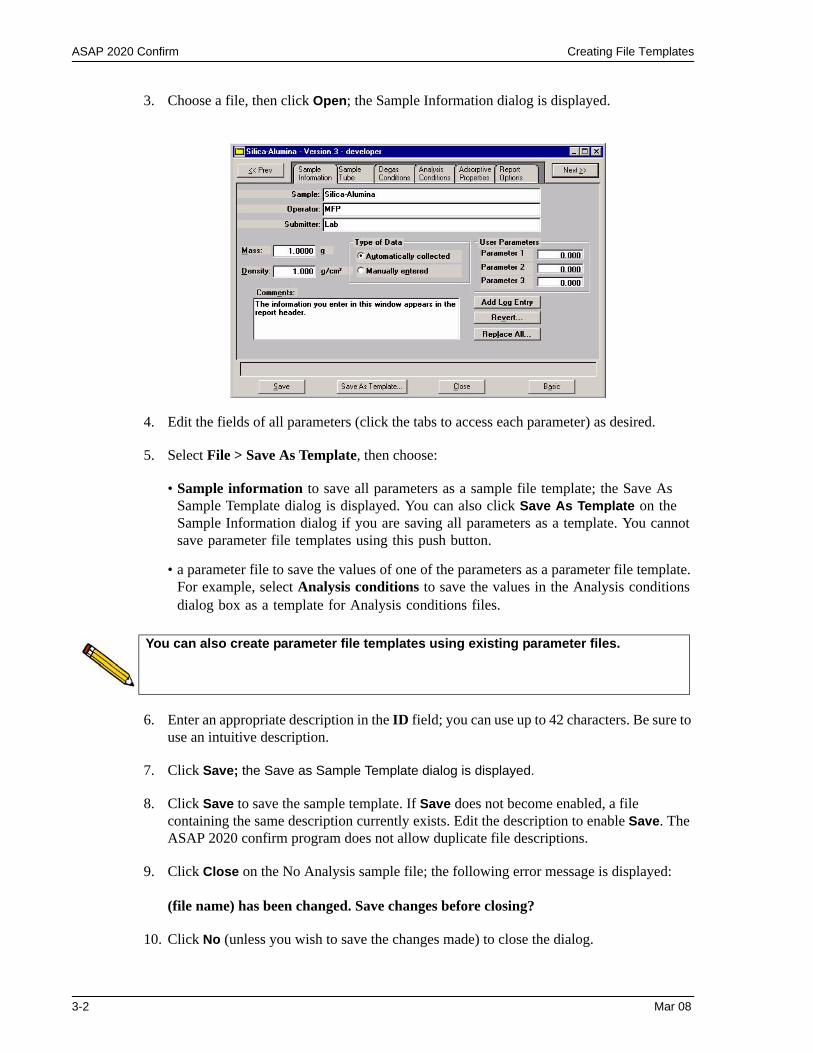
3. Choose a file, then click Open; the Sample Information dialog is displayed.
4. Edit the fields of all parameters (click the tabs to access each parameter) as desired.
5. Select File > Save As Template, then choose:
• Sample information to save all parameters as a sample file template; the Save As Sample Template dialog is displayed. You can also click Save As Template on the Sample Information dialog if you are saving all parameters as a template. You cannot save parameter file templates using this push button.
• a parameter file to save the values of one of the parameters as a parameter file template. For example, select Analysis conditions to save the values in the Analysis conditions dialog box as a template for Analysis conditions files.
6. Enter an appropriate description in the ID field; you can use up to 42 characters. Be sure to use an intuitive description.
7. Click Save; the Save as Sample Template dialog is displayed.
8. Click Save to save the sample template. If Save does not become enabled, a file containing the same description currently exists. Edit the description to enable Save. The ASAP 2020 confirm program does not allow duplicate file descriptions.
9. Click Close on the No Analysis sample file; the following error message is displayed:
(file name) has been changed. Save changes before closing?
10. Click No (unless you wish to save the changes made) to close the dialog.
You can also create parameter file templates using existing parameter files.
3-2 Mar 08
Creating Parameter Files ASAP 2020 Confirm
Creating Parameter Files
The following file types can exist as part of the sample information file, as well as individual parameter files:
• Sample tube• Degas conditions• Analysis conditions• Adsorptive properties• Report options
Having these files exist independently allows you to use them over and over again.
Several predefined parameter files are included with the ASAP 2020 Confirm program. Although these files may come close to the needs of your laboratory, you may wish to define additional ones. Or you can use a predefined file as a starting point. You can do this by creating a new file and then selecting Replace. A dialog is displayed so that you can select the existing parameter file. Then you can make any changes you need to make and the played.
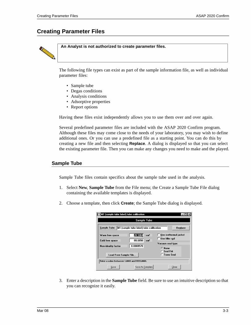
Sample Tube
Sample Tube files contain specifics about the sample tube used in the analysis.
1. Select New, Sample Tube from the File menu; the Create a Sample Tube File dialog containing the available templates is displayed.
2. Choose a template, then click Create; the Sample Tube dialog is displayed.
3. Enter a description in the Sample Tube field. Be sure to use an intuitive description so that you can recognize it easily.
An Analyst is not authorized to create parameter files.
Mar 08 3-3
ASAP 2020 Confirm Creating Parameter Files
4. Click Load from Sample File; the Open Sample Information File dialog is displayed.
5. Select the file you used in the blank run with this sample tube, then click Open to copy the warm and cold free space, and the non-ideality factor values into the Sample Tube dialog.
6. Select whether an isothermal jacket and/or filler rod is(are) being used.
7. If a vacuum seal of some type was used, select the appropriate option or leave the default of None selected.
8. Click Save; the Save As Sample Tube dialog is displayed.
9. Ensure that the description is as desired, then click Save to save the file and return to the Sample Tube file dialog. If Save is disabled, the description is a duplicate one and must be edited. The ASAP 2020 Confirm program does not allow duplicate descriptions.
10. Click Close to close the dialog box.
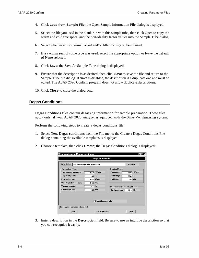
Degas Conditions
Degas Conditions files contain degassing information for sample preparation. These files apply only if your ASAP 2020 analyzer is equipped with the SmartVac degassing system.
Perform the following steps to create a degas conditions file:
1. Select New, Degas conditions from the File menu; the Create a Degas Conditions File dialog containing the available templates is displayed.
2. Choose a template, then click Create; the Degas Conditions dialog is displayed:
3. Enter a description in the Description field. Be sure to use an intuitive description so that you can recognize it easily.
3-4 Mar 08
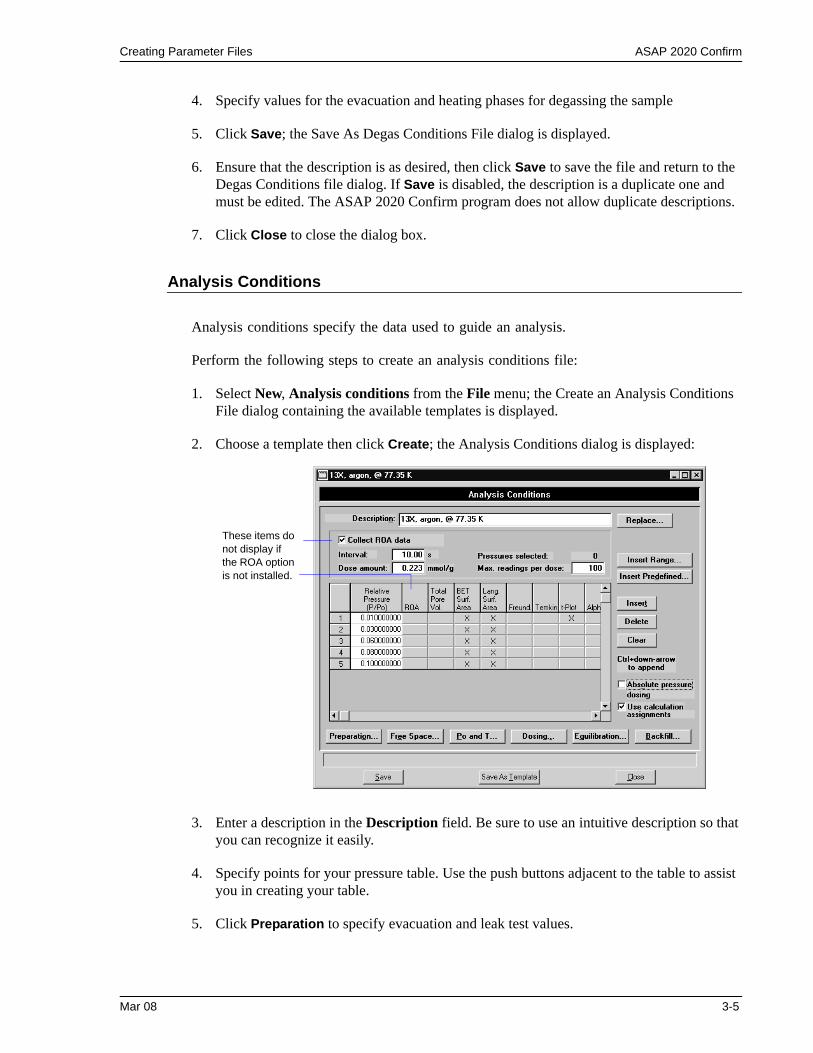
Creating Parameter Files ASAP 2020 Confirm
4. Specify values for the evacuation and heating phases for degassing the sample
5. Click Save; the Save As Degas Conditions File dialog is displayed.
6. Ensure that the description is as desired, then click Save to save the file and return to the Degas Conditions file dialog. If Save is disabled, the description is a duplicate one and must be edited. The ASAP 2020 Confirm program does not allow duplicate descriptions.
7. Click Close to close the dialog box.
Analysis Conditions
Analysis conditions specify the data used to guide an analysis.
Perform the following steps to create an analysis conditions file:
1. Select New, Analysis conditions from the File menu; the Create an Analysis Conditions File dialog containing the available templates is displayed.
2. Choose a template then click Create; the Analysis Conditions dialog is displayed:
3. Enter a description in the Description field. Be sure to use an intuitive description so that you can recognize it easily.
4. Specify points for your pressure table. Use the push buttons adjacent to the table to assist you in creating your table.
5. Click Preparation to specify evacuation and leak test values.
These items do not display if the ROA option is not installed.
Mar 08 3-5
ASAP 2020 Confirm Creating Parameter Files
6. Click Free Space to specify how the free space is to be measured.
7. Click Po and T to specify how the saturation pressure (Po) is to be measured and the analysis bath temperature. If you select Absolute pressure dosing, options 1 through 5 are disabled. The Po will be calculated using the analysis bath temperature; enter the appropriate temperature in the field provided.
8. Click Dosing to specify dosing options.
9. Click Equilibration to specify the equilibration interval and its delay time.
10. Click Backfill to specify backfill options.
11. If you wish to use absolute dosing, click the Absolute pressure dosing option.
12. Click Save; the Save As Analysis Conditions File dialog is displayed.
13. Ensure that the description is as desired, then click Save to save the file and return to the Analysis Conditions file dialog. If Save is disabled, the description is a duplicate one and must be edited. The ASAP 2020 Confirm program does not allow duplicate descriptions.
14. Click Close to close the dialog.
3-6 Mar 08
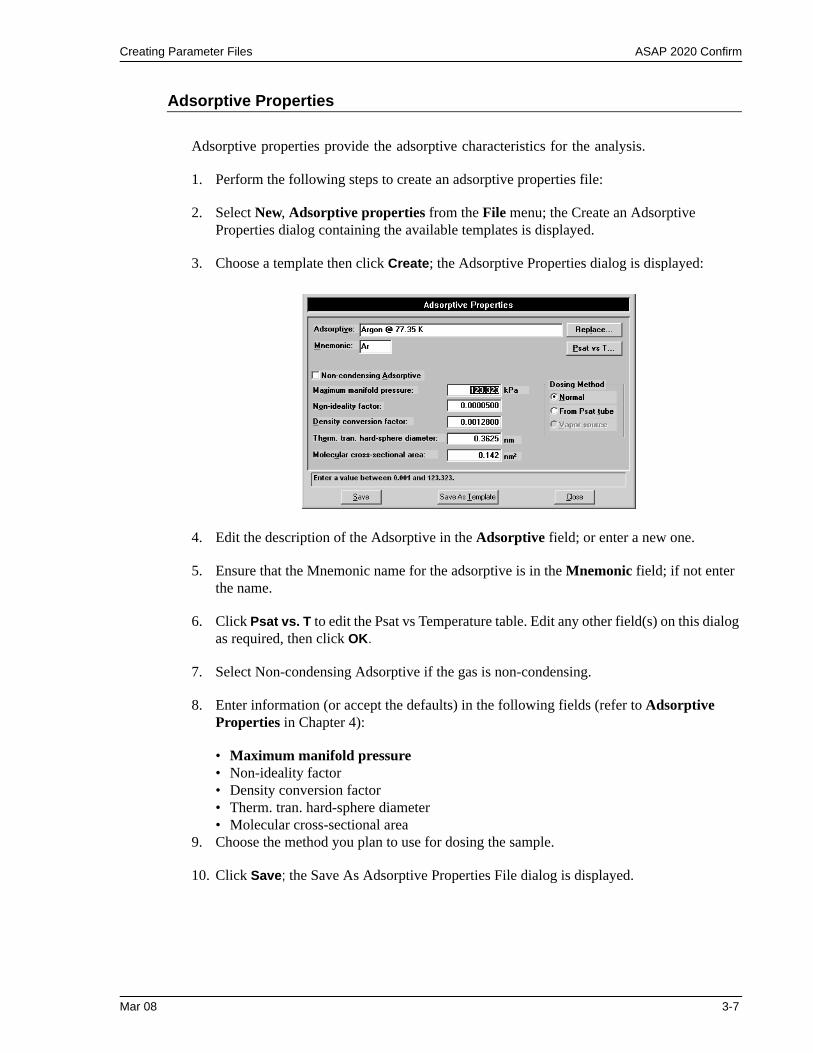
Creating Parameter Files ASAP 2020 Confirm
Adsorptive Properties
Adsorptive properties provide the adsorptive characteristics for the analysis.
1. Perform the following steps to create an adsorptive properties file:
2. Select New, Adsorptive properties from the File menu; the Create an Adsorptive Properties dialog containing the available templates is displayed.
3. Choose a template then click Create; the Adsorptive Properties dialog is displayed:
4. Edit the description of the Adsorptive in the Adsorptive field; or enter a new one.
5. Ensure that the Mnemonic name for the adsorptive is in the Mnemonic field; if not enter the name.
6. Click Psat vs. T to edit the Psat vs Temperature table. Edit any other field(s) on this dialog as required, then click OK.
7. Select Non-condensing Adsorptive if the gas is non-condensing.
8. Enter information (or accept the defaults) in the following fields (refer to Adsorptive Properties in Chapter 4):
• Maximum manifold pressure• Non-ideality factor• Density conversion factor• Therm. tran. hard-sphere diameter• Molecular cross-sectional area
9. Choose the method you plan to use for dosing the sample.
10. Click Save; the Save As Adsorptive Properties File dialog is displayed.
Mar 08 3-7
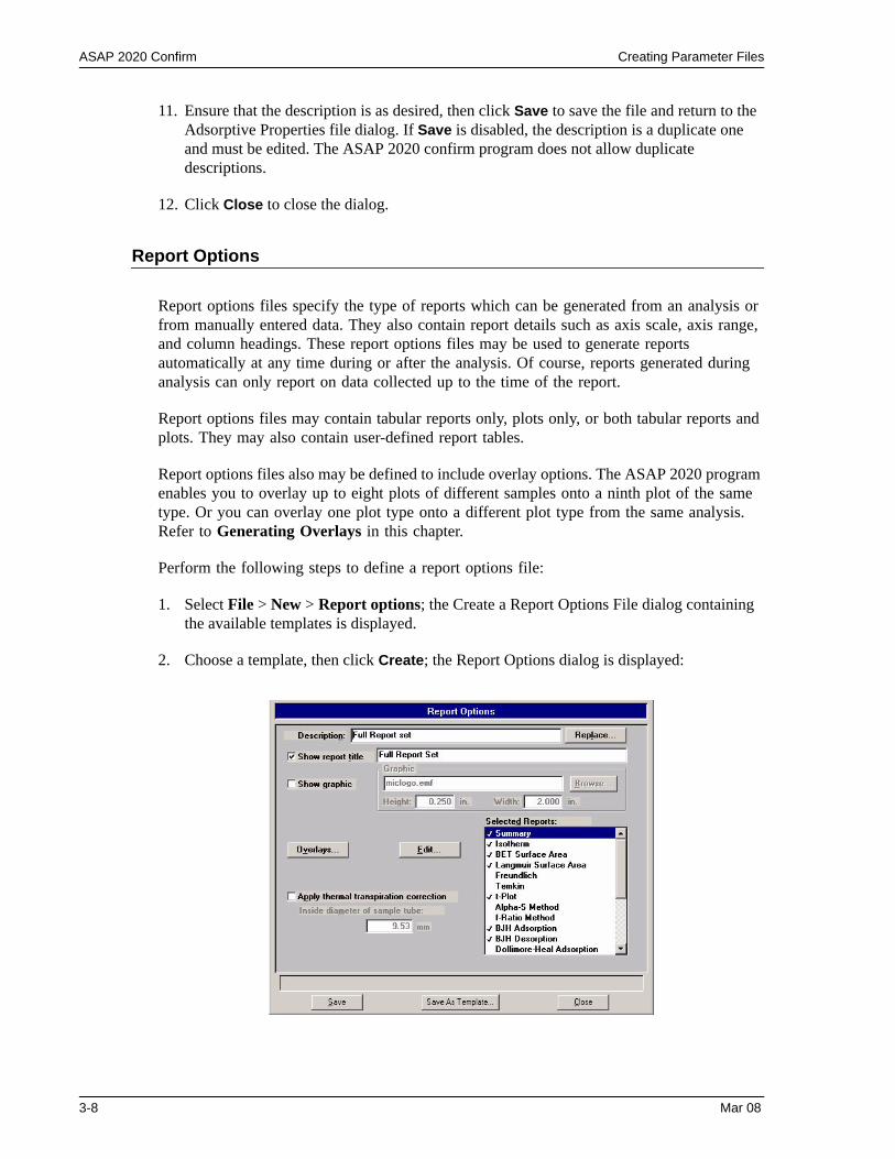
ASAP 2020 Confirm Creating Parameter Files
11. Ensure that the description is as desired, then click Save to save the file and return to the Adsorptive Properties file dialog. If Save is disabled, the description is a duplicate one and must be edited. The ASAP 2020 confirm program does not allow duplicate descriptions.
12. Click Close to close the dialog.
Report Options
Report options files specify the type of reports which can be generated from an analysis or from manually entered data. They also contain report details such as axis scale, axis range, and column headings. These report options files may be used to generate reports automatically at any time during or after the analysis. Of course, reports generated during analysis can only report on data collected up to the time of the report.
Report options files may contain tabular reports only, plots only, or both tabular reports and plots. They may also contain user-defined report tables.
Report options files also may be defined to include overlay options. The ASAP 2020 program enables you to overlay up to eight plots of different samples onto a ninth plot of the same type. Or you can overlay one plot type onto a different plot type from the same analysis. Refer to Generating Overlays in this chapter.
Perform the following steps to define a report options file:
1. Select File > New > Report options; the Create a Report Options File dialog containing the available templates is displayed.
2. Choose a template, then click Create; the Report Options dialog is displayed:
3-8 Mar 08
Creating Parameter Files ASAP 2020 Confirm
3. Enter a description (up to 42 characters) in the Description field. Enter an identifier that gives a more intuitive description of the files contents. For example, BJH Adsorption Report Options.
4. Select Show report title and enter the title you wish to appear at the top of the report. Or deselect this option if you prefer not to have a report title.
5. If you wish to compare the same type of graph from multiple files, click Overlays and choose the files. Then be sure you edit the graph from the Selected Reports window and choose Samples from the Overlay drop-down list.
6. The reports that may be generated are listed in the Selected Reports list. Select reports by double-clicking on the desired report, or highlight the report and press the spacebar. Reports are deselected in the same manner. A report is selected when it is preceded by a check mark. You can edit details of some reports by highlighting the desired report and clicking Edit.
7. Click Save; the Save As Report Options File dialog is displayed.
8. Ensure that the description is as desired, then click Save to save the file and return to the Report Options file dialog. If it is disabled, the description is a duplicate one and must be edited.
9. Click Close to close the dialog.
If your company logo exists as a bitmap (bmp) or enhanced metafile (emf), you can have it display in the report header by selecting Show graphic. Click Browse to select the file; use the Height and Width fields to specify the size.
Mar 08 3-9
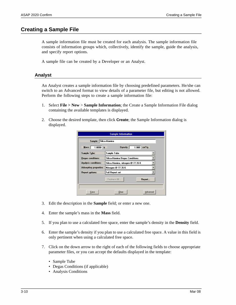
ASAP 2020 Confirm Creating a Sample File
Creating a Sample File
A sample information file must be created for each analysis. The sample information file consists of information groups which, collectively, identify the sample, guide the analysis, and specify report options.
A sample file can be created by a Developer or an Analyst.
Analyst
An Analyst creates a sample information file by choosing predefined parameters. He/she can switch to an Advanced format to view details of a parameter file, but editing is not allowed. Perform the following steps to create a sample information file:
1. Select File > New > Sample Information; the Create a Sample Information File dialog containing the available templates is displayed.
2. Choose the desired template, then click Create; the Sample Information dialog is displayed.
3. Edit the description in the Sample field; or enter a new one.
4. Enter the sample’s mass in the Mass field.
5. If you plan to use a calculated free space, enter the sample’s density in the Density field.
6. Enter the sample’s density if you plan to use a calculated free space. A value in this field is only pertinent when using a calculated free space.
7. Click on the down arrow to the right of each of the following fields to choose appropriate parameter files, or you can accept the defaults displayed in the template:
• Sample Tube• Degas Conditions (if applicable)• Analysis Conditions
3-10 Mar 08
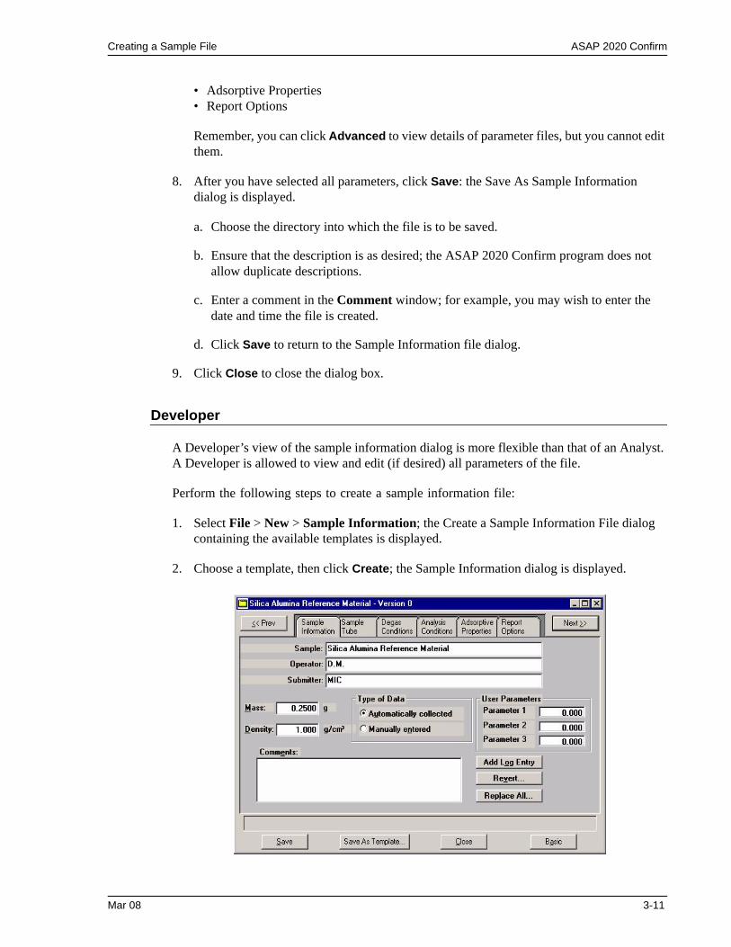
Creating a Sample File ASAP 2020 Confirm
• Adsorptive Properties• Report Options
Remember, you can click Advanced to view details of parameter files, but you cannot edit them.
8. After you have selected all parameters, click Save: the Save As Sample Information dialog is displayed.
a. Choose the directory into which the file is to be saved.
b. Ensure that the description is as desired; the ASAP 2020 Confirm program does not allow duplicate descriptions.
c. Enter a comment in the Comment window; for example, you may wish to enter the date and time the file is created.
d. Click Save to return to the Sample Information file dialog.
9. Click Close to close the dialog box.
Developer
A Developer’s view of the sample information dialog is more flexible than that of an Analyst. A Developer is allowed to view and edit (if desired) all parameters of the file.
Perform the following steps to create a sample information file:
1. Select File > New > Sample Information; the Create a Sample Information File dialog containing the available templates is displayed.
2. Choose a template, then click Create; the Sample Information dialog is displayed.
Mar 08 3-11
ASAP 2020 Confirm Creating a Sample File
3. Edit (or enter) the description in the Sample field; you can use up to 42 characters.
4. In the Operator field, enter the name of the Analyst who will be performing the analysis.
5. In the Submitter field, enter the name of the department, company, etc. submitting the sample for analysis.
6. Enter the mass of the sample in the Mass field; this value can be edited later if desired.
7. Enter the sample’s density if you plan to use a calculated free space. A value in this field is only pertinent when using a calculated free space.
8. Choose whether you are going to enter data or have it automatically collected.
9. If you plan to report statistical process control (SPC) information, enter appropriate information. These are user-definable parameters that can be entered and tracked along with other statistical process control data; refer to Edit Labels, page 7-3 for additional information on these parameters.
10. After you complete the Sample Information dialog, click on the parameter tabs to open associated dialogs and edit as desired. Instructions for completing these dialogs are explained in Creating Parameter Files beginning on page 3-3.
11. After you have completed all parameters, click Save: the Save As Sample Information dialog is displayed.
a. Choose the directory into which the file is to be saved.
b. Edit the description; the ASAP 2020 Confirm program does not allow duplicate descriptions.
c. Enter a comment in the Comment window; for example, you may wish to enter the date and time the file is created.
d. Click Save to complete the save operation and return to the Sample Information file dialog.
12. Click Close to close the dialog.
3-12 Mar 08
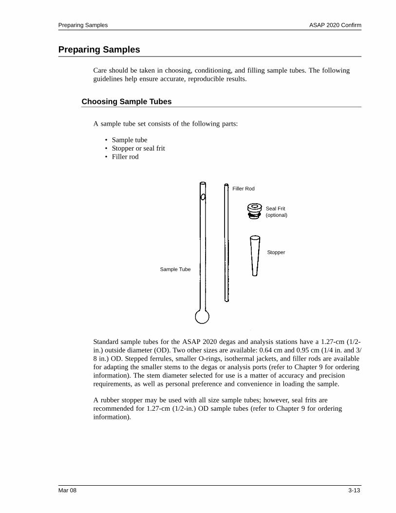
Preparing Samples ASAP 2020 Confirm
Preparing Samples
Care should be taken in choosing, conditioning, and filling sample tubes. The following guidelines help ensure accurate, reproducible results.
Choosing Sample Tubes
A sample tube set consists of the following parts:
• Sample tube• Stopper or seal frit• Filler rod
Standard sample tubes for the ASAP 2020 degas and analysis stations have a 1.27-cm (1/2-in.) outside diameter (OD). Two other sizes are available: 0.64 cm and 0.95 cm (1/4 in. and 3/8 in.) OD. Stepped ferrules, smaller O-rings, isothermal jackets, and filler rods are available for adapting the smaller stems to the degas or analysis ports (refer to Chapter 9 for ordering information). The stem diameter selected for use is a matter of accuracy and precision requirements, as well as personal preference and convenience in loading the sample.
A rubber stopper may be used with all size sample tubes; however, seal frits are recommended for 1.27-cm (1/2-in.) OD sample tubes (refer to Chapter 9 for ordering information).
Sample Tube
Filler Rod
Stopper
Seal Frit (optional)
Mar 08 3-13
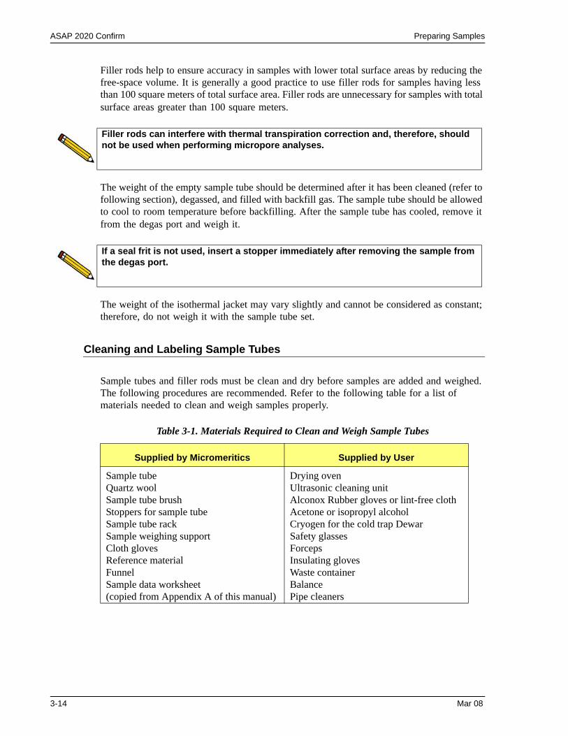
ASAP 2020 Confirm Preparing Samples
Filler rods help to ensure accuracy in samples with lower total surface areas by reducing the free-space volume. It is generally a good practice to use filler rods for samples having less than 100 square meters of total surface area. Filler rods are unnecessary for samples with total surface areas greater than 100 square meters.
The weight of the empty sample tube should be determined after it has been cleaned (refer to following section), degassed, and filled with backfill gas. The sample tube should be allowed to cool to room temperature before backfilling. After the sample tube has cooled, remove it from the degas port and weigh it.
The weight of the isothermal jacket may vary slightly and cannot be considered as constant; therefore, do not weigh it with the sample tube set.
Cleaning and Labeling Sample Tubes
Sample tubes and filler rods must be clean and dry before samples are added and weighed. The following procedures are recommended. Refer to the following table for a list of materials needed to clean and weigh samples properly.
Table 3-1. Materials Required to Clean and Weigh Sample Tubes
Filler rods can interfere with thermal transpiration correction and, therefore, should not be used when performing micropore analyses.
If a seal frit is not used, insert a stopper immediately after removing the sample from the degas port.
Supplied by Micromeritics Supplied by User
Sample tubeQuartz woolSample tube brushStoppers for sample tubeSample tube rackSample weighing supportCloth glovesReference materialFunnelSample data worksheet (copied from Appendix A of this manual)
Drying ovenUltrasonic cleaning unitAlconox Rubber gloves or lint-free clothAcetone or isopropyl alcoholCryogen for the cold trap DewarSafety glassesForcepsInsulating glovesWaste containerBalancePipe cleaners
3-14 Mar 08
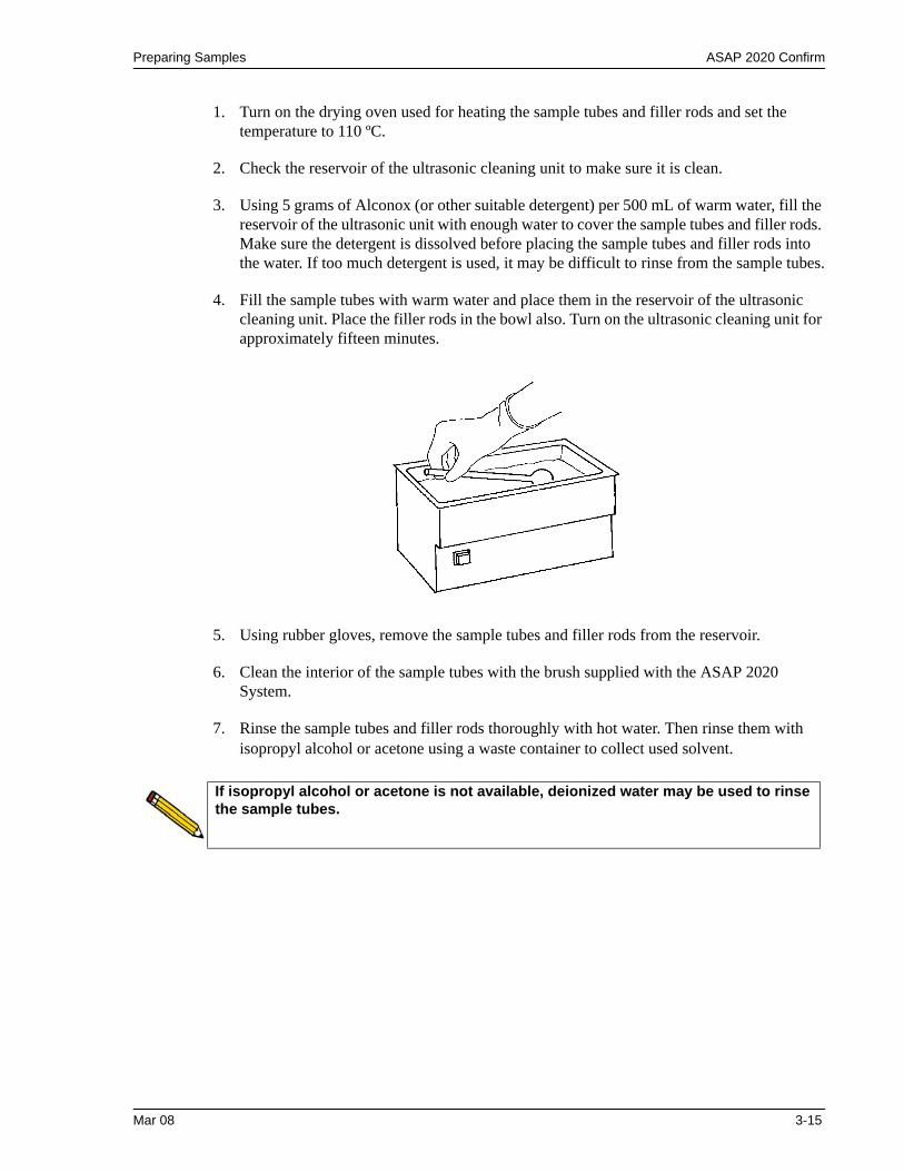
Preparing Samples ASAP 2020 Confirm
1. Turn on the drying oven used for heating the sample tubes and filler rods and set the temperature to 110 ºC.
2. Check the reservoir of the ultrasonic cleaning unit to make sure it is clean.
3. Using 5 grams of Alconox (or other suitable detergent) per 500 mL of warm water, fill the reservoir of the ultrasonic unit with enough water to cover the sample tubes and filler rods. Make sure the detergent is dissolved before placing the sample tubes and filler rods into the water. If too much detergent is used, it may be difficult to rinse from the sample tubes.
4. Fill the sample tubes with warm water and place them in the reservoir of the ultrasonic cleaning unit. Place the filler rods in the bowl also. Turn on the ultrasonic cleaning unit for approximately fifteen minutes.
5. Using rubber gloves, remove the sample tubes and filler rods from the reservoir.
6. Clean the interior of the sample tubes with the brush supplied with the ASAP 2020 System.
7. Rinse the sample tubes and filler rods thoroughly with hot water. Then rinse them with isopropyl alcohol or acetone using a waste container to collect used solvent.
If isopropyl alcohol or acetone is not available, deionized water may be used to rinse the sample tubes.
Mar 08 3-15
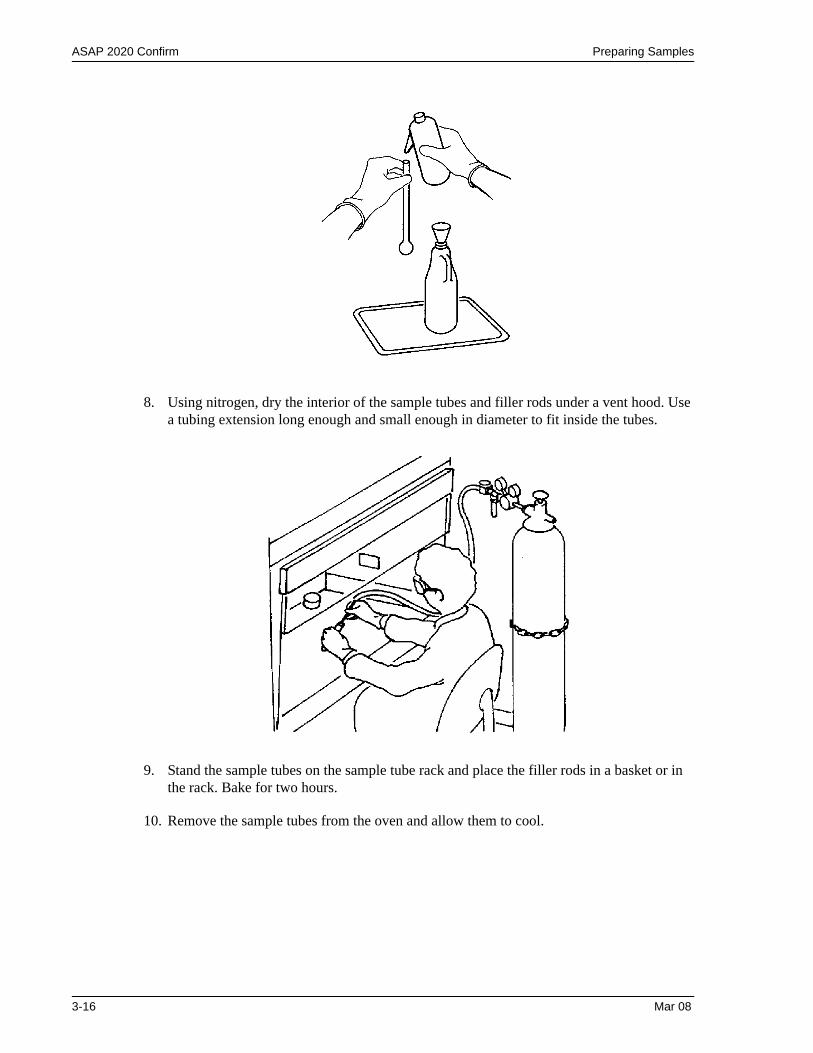
ASAP 2020 Confirm Preparing Samples
8. Using nitrogen, dry the interior of the sample tubes and filler rods under a vent hood. Use a tubing extension long enough and small enough in diameter to fit inside the tubes.
9. Stand the sample tubes on the sample tube rack and place the filler rods in a basket or in the rack. Bake for two hours.
10. Remove the sample tubes from the oven and allow them to cool.
3-16 Mar 08
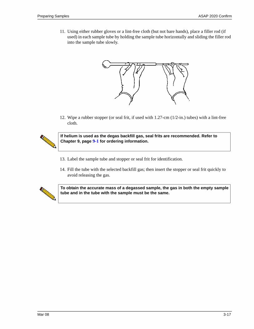
Preparing Samples ASAP 2020 Confirm
11. Using either rubber gloves or a lint-free cloth (but not bare hands), place a filler rod (if used) in each sample tube by holding the sample tube horizontally and sliding the filler rod into the sample tube slowly.
12. Wipe a rubber stopper (or seal frit, if used with 1.27-cm (1/2-in.) tubes) with a lint-free cloth.
13. Label the sample tube and stopper or seal frit for identification.
14. Fill the tube with the selected backfill gas; then insert the stopper or seal frit quickly to avoid releasing the gas.
If helium is used as the degas backfill gas, seal frits are recommended. Refer to Chapter 9, page 9-1 for ordering information.
To obtain the accurate mass of a degassed sample, the gas in both the empty sample tube and in the tube with the sample must be the same.
Mar 08 3-17
ASAP 2020 Confirm Preparing Samples
Determining Amount of Sample to Use
Clean, dry sample tubes are essential for accurate results. How much sample to use can be determined best by experiment. In general, a sample providing 40 to 120 square meters of total surface area is recommended for nitrogen analysis. Less than this may cause variability of results; considerably more than this extends unnecessarily the time required for analysis.
Smaller quantities are required for samples having high surface areas. These samples require careful weighing after degassing because a small error may represent a considerable percent of total weight. Proper weighing techniques are most important in this case. Use no less than 100 mg to reduce the effect of weighing errors.
Care should be taken when loading powders; the accessory funnel is useful for this purpose. Large granules or chunks may be loaded with forceps.
Determining the Mass of the Sample
Analysis results are expressed in units of surface area per gram of sample; therefore, the true mass of the sample must be known. Carefully weigh each sample tube set and sample as described below.
1. Write the Sample Tube number on the Sample Data Worksheet. (A Sample Data Worksheet, which you may copy, is included in Appendix A.)
2. Place the sample weighing support on the balance. Tare the balance and allow it to stabilize at zero (0).
3. Place the sample tube set (sample tube, stopper or seal frit, and filler rod, if used) on the sample support. Record the stabilized weight on the Sample Data Worksheet as Mass of empty sample tube. Remove the sample support and sample tube set from the balance.
4. Place a sample container onto the balance. Tare the balance and allow it to stabilize at zero (0).
5. Slowly add the sample to the sample container.
6. Remove the rubber stopper or seal frit and filler rod from the sample tube.
Avoid touching the sample with your fingers because oils may be transferred to the sample and can alter results or create degassing problems.
Do not touch the sample or filler rod with bare hands while performing the next six steps. Doing so could affect the accuracy of results.
3-18 Mar 08
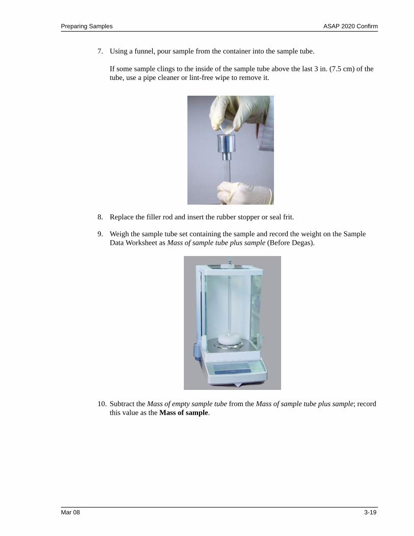
Preparing Samples ASAP 2020 Confirm
7. Using a funnel, pour sample from the container into the sample tube.
If some sample clings to the inside of the sample tube above the last 3 in. (7.5 cm) of the tube, use a pipe cleaner or lint-free wipe to remove it.
8. Replace the filler rod and insert the rubber stopper or seal frit.
9. Weigh the sample tube set containing the sample and record the weight on the Sample Data Worksheet as Mass of sample tube plus sample (Before Degas).
10. Subtract the Mass of empty sample tube from the Mass of sample tube plus sample; record this value as the Mass of sample.
Mar 08 3-19
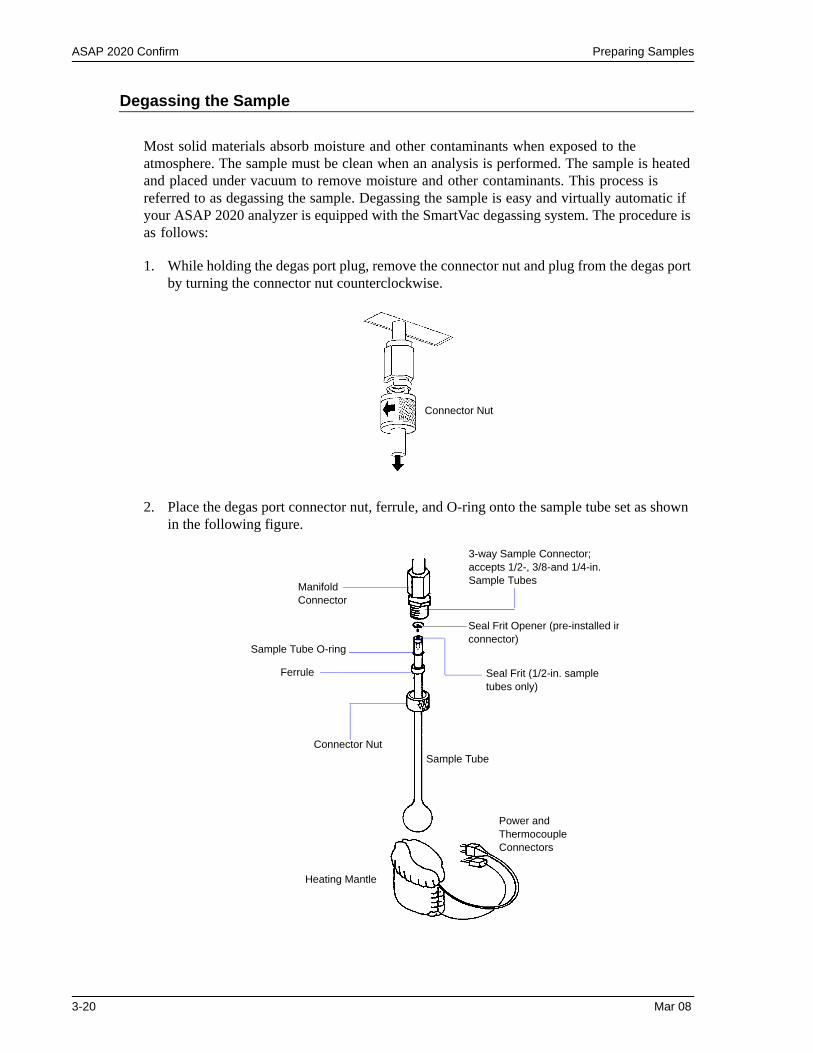
ASAP 2020 Confirm Preparing Samples
Degassing the Sample
Most solid materials absorb moisture and other contaminants when exposed to the atmosphere. The sample must be clean when an analysis is performed. The sample is heated and placed under vacuum to remove moisture and other contaminants. This process is referred to as degassing the sample. Degassing the sample is easy and virtually automatic if your ASAP 2020 analyzer is equipped with the SmartVac degassing system. The procedure is as follows:
1. While holding the degas port plug, remove the connector nut and plug from the degas port by turning the connector nut counterclockwise.
2. Place the degas port connector nut, ferrule, and O-ring onto the sample tube set as shown in the following figure.
Connector Nut
Manifold Connector
Sample Tube O-ring
Connector Nut
Seal Frit Opener (pre-installed inconnector)
Ferrule
3-way Sample Connector; accepts 1/2-, 3/8-and 1/4-in. Sample Tubes
Seal Frit (1/2-in. sample tubes only)
Sample Tube
Heating Mantle
Power and Thermocouple Connectors
3-20 Mar 08
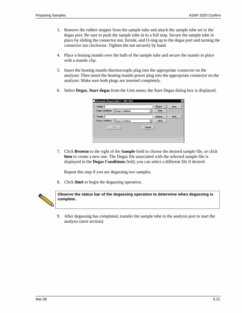
Preparing Samples ASAP 2020 Confirm
3. Remove the rubber stopper from the sample tube and attach the sample tube set to the degas port. Be sure to push the sample tube in to a full stop. Secure the sample tube in place by sliding the connector nut, ferrule, and O-ring up to the degas port and turning the connector nut clockwise. Tighten the nut securely by hand.
4. Place a heating mantle over the bulb of the sample tube and secure the mantle in place with a mantle clip.
5. Insert the heating mantle thermocouple plug into the appropriate connector on the analyzer. Then insert the heating mantle power plug into the appropriate connector on the analyzer. Make sure both plugs are inserted completely.
6. Select Degas, Start degas from the Unit menu; the Start Degas dialog box is displayed.
7. Click Browse to the right of the Sample field to choose the desired sample file, or click New to create a new one. The Degas file associated with the selected sample file is displayed in the Degas Conditions field; you can select a different file if desired.
Repeat this step if you are degassing two samples.
8. Click Start to begin the degassing operation.
9. After degassing has completed, transfer the sample tube to the analysis port to start the analysis (next section).
Observe the status bar of the degassing operation to determine when degassing is complete.
Mar 08 3-21
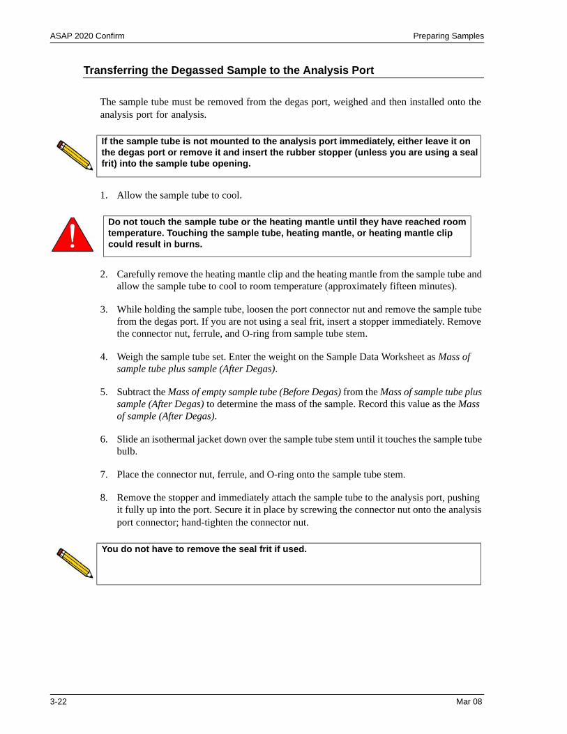
ASAP 2020 Confirm Preparing Samples
Transferring the Degassed Sample to the Analysis Port
The sample tube must be removed from the degas port, weighed and then installed onto the analysis port for analysis.
1. Allow the sample tube to cool.
2. Carefully remove the heating mantle clip and the heating mantle from the sample tube and allow the sample tube to cool to room temperature (approximately fifteen minutes).
3. While holding the sample tube, loosen the port connector nut and remove the sample tube from the degas port. If you are not using a seal frit, insert a stopper immediately. Remove the connector nut, ferrule, and O-ring from sample tube stem.
4. Weigh the sample tube set. Enter the weight on the Sample Data Worksheet as Mass of sample tube plus sample (After Degas).
5. Subtract the Mass of empty sample tube (Before Degas) from the Mass of sample tube plus sample (After Degas) to determine the mass of the sample. Record this value as the Mass of sample (After Degas).
6. Slide an isothermal jacket down over the sample tube stem until it touches the sample tube bulb.
7. Place the connector nut, ferrule, and O-ring onto the sample tube stem.
8. Remove the stopper and immediately attach the sample tube to the analysis port, pushing it fully up into the port. Secure it in place by screwing the connector nut onto the analysis port connector; hand-tighten the connector nut.
If the sample tube is not mounted to the analysis port immediately, either leave it on the degas port or remove it and insert the rubber stopper (unless you are using a seal frit) into the sample tube opening.
Do not touch the sample tube or the heating mantle until they have reached room temperature. Touching the sample tube, heating mantle, or heating mantle clip could result in burns.
You do not have to remove the seal frit if used.
3-22 Mar 08
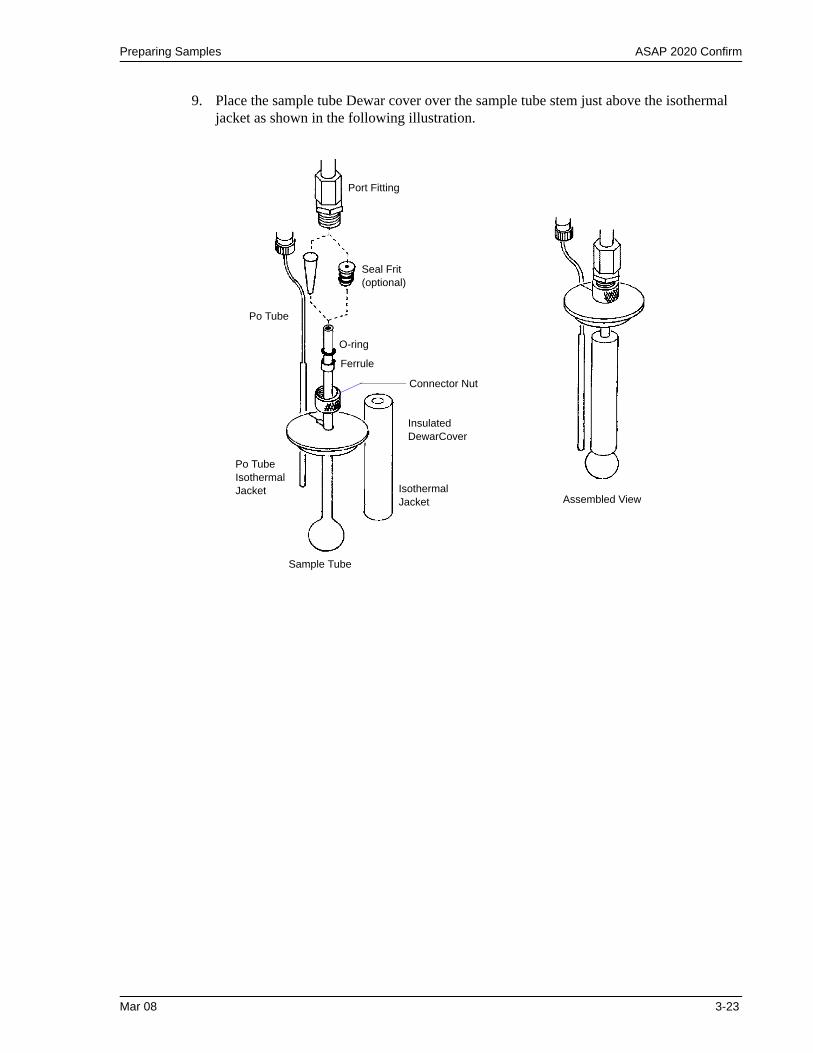
Preparing Samples ASAP 2020 Confirm
9. Place the sample tube Dewar cover over the sample tube stem just above the isothermal jacket as shown in the following illustration.
Port Fitting
Seal Frit (optional)
Connector Nut
Insulated DewarCover
Isothermal Jacket
Sample Tube
Po Tube Isothermal Jacket
Po Tube
Ferrule
O-ring
Assembled View
Mar 08 3-23
ASAP 2020 Confirm Installing Dewars
Installing Dewars
Precautions
Always handle Dewars with care. Any product incorporating a vacuum is a potential safety hazard and should be treated with caution.
We recommend the following be observed when handling Dewars containing liquefied gases:
• Protect yourself by wearing 1) goggles (or a face shield), 2) an insulated or rubber apron, and 3) insulated gloves.
• When pouring liquefied gases from one container to another: 1) cool the receiving container gradually to minimize thermal shock, 2) pour the liquefied gas slowly to prevent splashing, and 3) vent the receiving container to the atmosphere.
• Use a plastic stirring rod when stirring substances in a Dewar containing liquefied gases (or other materials of extremely low temperature). Do not use a glass or metal stirring rod unless it is coated with some form of protective coating.
• Do not handle heavy objects above the Dewar. If unavoidable, place a protective cover over the Dewar’s opening. If an object of sufficient weight is accidentally dropped into the Dewar, shattering may occur.
3-24 Mar 08
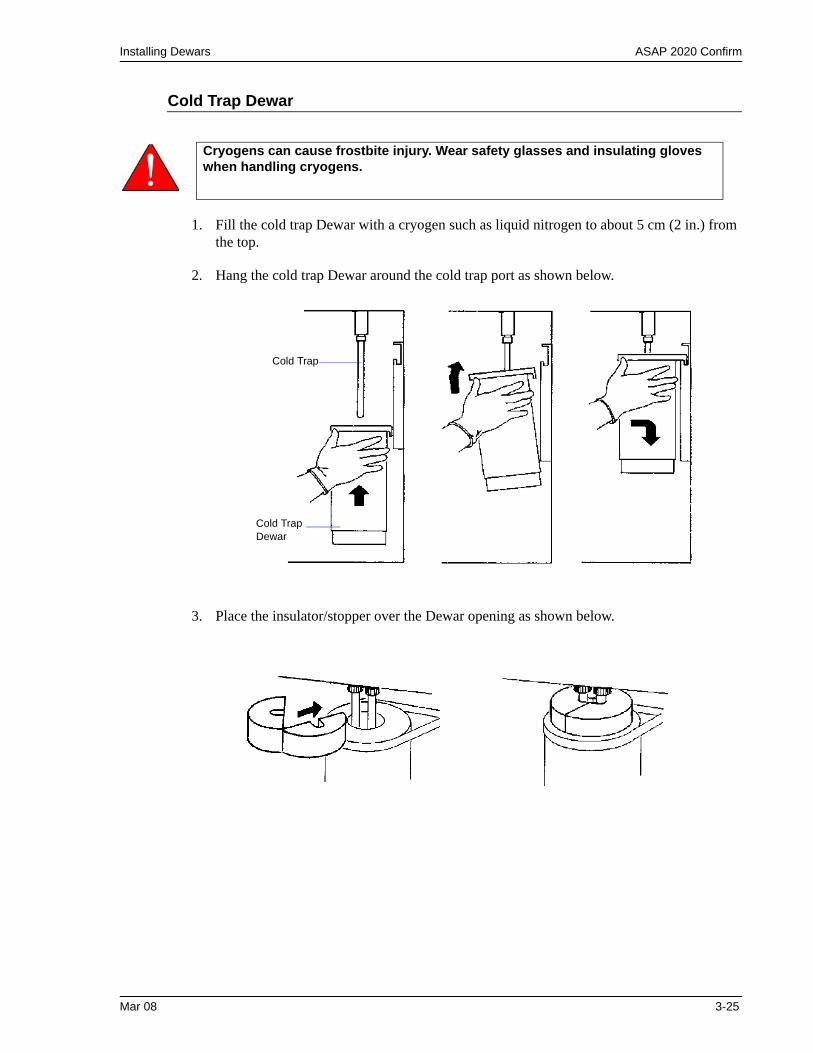
Installing Dewars ASAP 2020 Confirm
Cold Trap Dewar
1. Fill the cold trap Dewar with a cryogen such as liquid nitrogen to about 5 cm (2 in.) from the top.
2. Hang the cold trap Dewar around the cold trap port as shown below.
3. Place the insulator/stopper over the Dewar opening as shown below.
Cryogens can cause frostbite injury. Wear safety glasses and insulating gloves when handling cryogens.
Cold Trap
Cold Trap Dewar
Mar 08 3-25
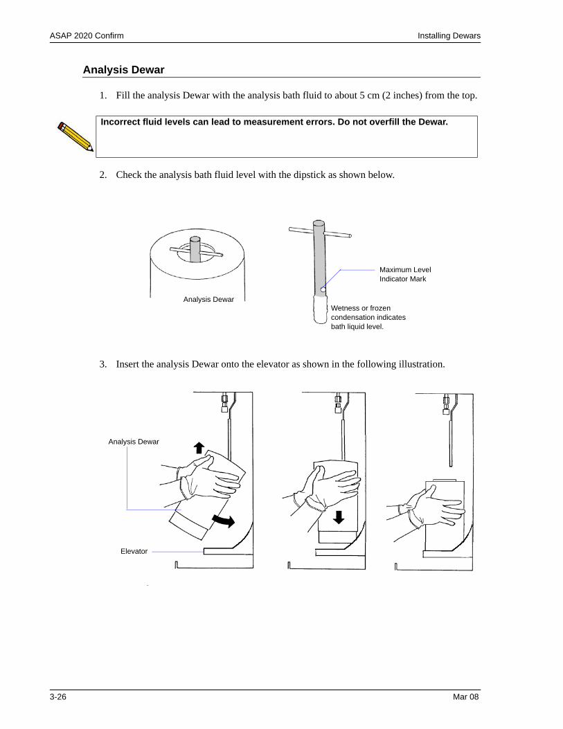
ASAP 2020 Confirm Installing Dewars
Analysis Dewar
1. Fill the analysis Dewar with the analysis bath fluid to about 5 cm (2 inches) from the top.
2. Check the analysis bath fluid level with the dipstick as shown below.
3. Insert the analysis Dewar onto the elevator as shown in the following illustration.
Incorrect fluid levels can lead to measurement errors. Do not overfill the Dewar.
Maximum Level Indicator Mark
Wetness or frozen condensation indicates bath liquid level.
Analysis Dewar
Analysis Dewar
Elevator
3-26 Mar 08
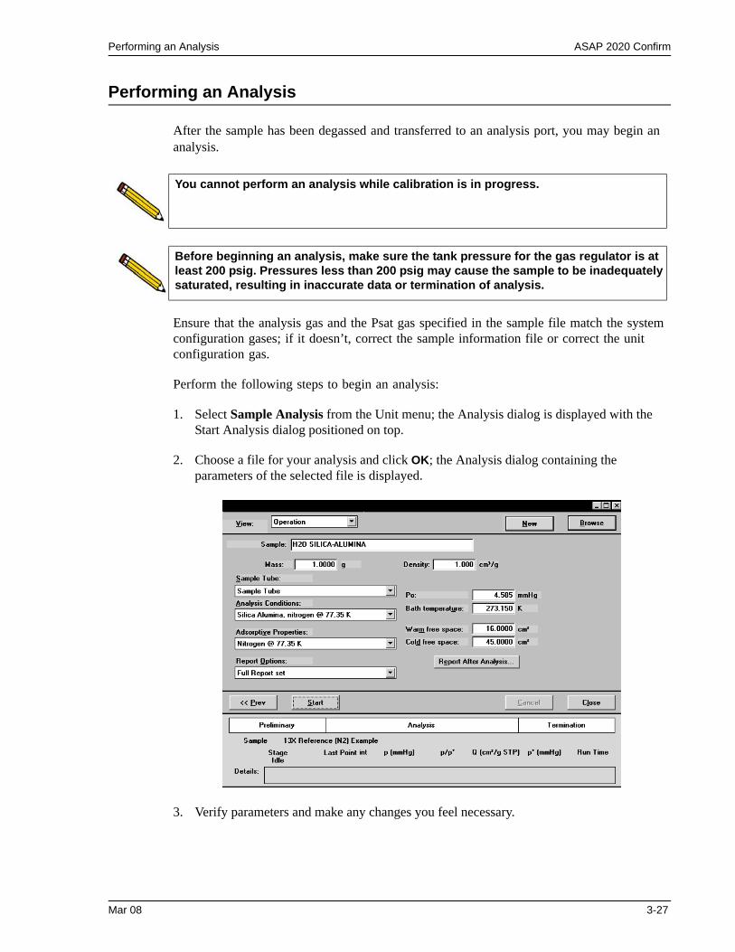
Performing an Analysis ASAP 2020 Confirm
Performing an Analysis
After the sample has been degassed and transferred to an analysis port, you may begin an analysis.
Ensure that the analysis gas and the Psat gas specified in the sample file match the system configuration gases; if it doesn’t, correct the sample information file or correct the unit configuration gas.
Perform the following steps to begin an analysis:
1. Select Sample Analysis from the Unit menu; the Analysis dialog is displayed with the Start Analysis dialog positioned on top.
2. Choose a file for your analysis and click OK; the Analysis dialog containing the parameters of the selected file is displayed.
3. Verify parameters and make any changes you feel necessary.
You cannot perform an analysis while calibration is in progress.
Before beginning an analysis, make sure the tank pressure for the gas regulator is at least 200 psig. Pressures less than 200 psig may cause the sample to be inadequately saturated, resulting in inaccurate data or termination of analysis.
Mar 08 3-27
ASAP 2020 Confirm Performing an Analysis
4. To generate a report automatically after the analysis, click Report After Analysis and choose report output options. You can generate reports to the screen (Preview) or directly to a printer. A Developer can also Export data to a file name; the Export option is unavailable for an Analyst.
5. Click Start to begin the analysis; a Logon dialog is displayed. The purpose of this dialog is to ensure that the person logged onto the system is actually performing the analysis. Enter your password and click OK to close the dialog and begin the analysis; a graphical representation of the data as collected is displayed.
6. Click Next to perform another analysis; the first view of the Analysis dialog is displayed.
If you choose to print reports to the screen, many options for manipulating and customizing your reports are provided from the Report window. You can also print to a printer from the Report window. Or if you prefer, you can choose not to generate reports after an analysis and generate them later using the Start Report command on the Reports menu.
Make sure the elevator is all the way down. If it is not all the way down, hazardous conditions can result.
3-28 Mar 08
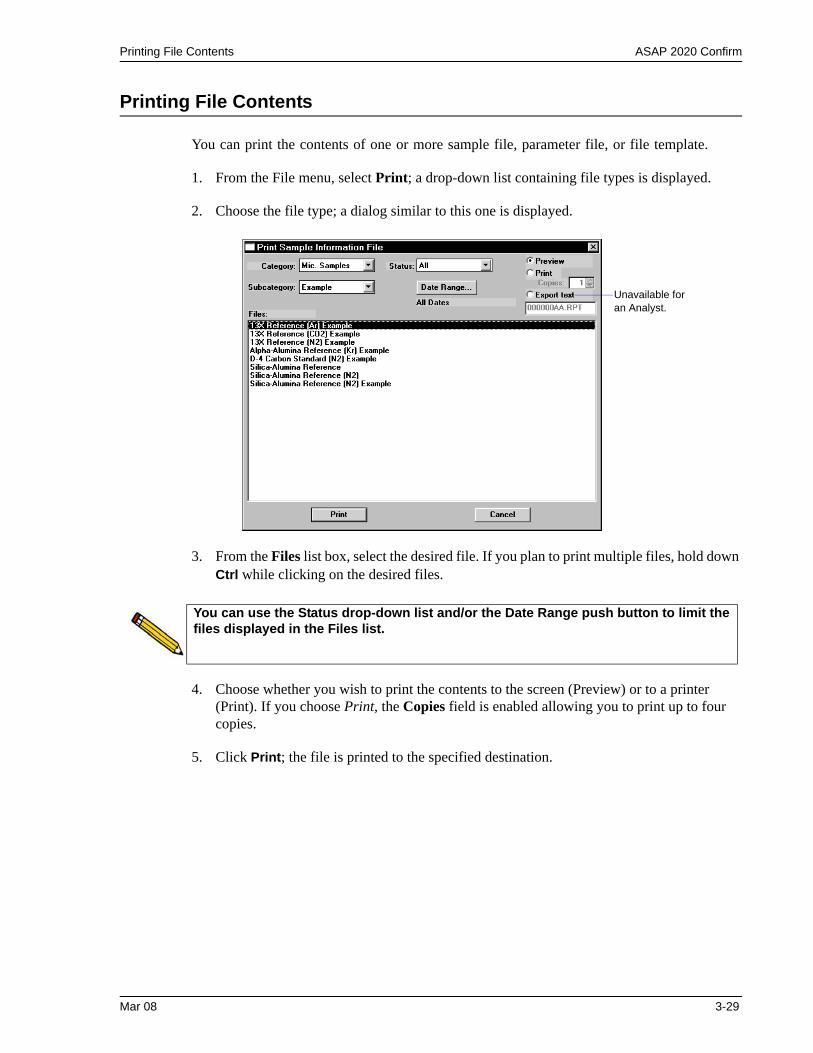
Printing File Contents ASAP 2020 Confirm
Printing File Contents
You can print the contents of one or more sample file, parameter file, or file template.
1. From the File menu, select Print; a drop-down list containing file types is displayed.
2. Choose the file type; a dialog similar to this one is displayed.
3. From the Files list box, select the desired file. If you plan to print multiple files, hold down Ctrl while clicking on the desired files.
4. Choose whether you wish to print the contents to the screen (Preview) or to a printer (Print). If you choose Print, the Copies field is enabled allowing you to print up to four copies.
5. Click Print; the file is printed to the specified destination.
Unavailable for an Analyst.
You can use the Status drop-down list and/or the Date Range push button to limit the files displayed in the Files list.
Mar 08 3-29
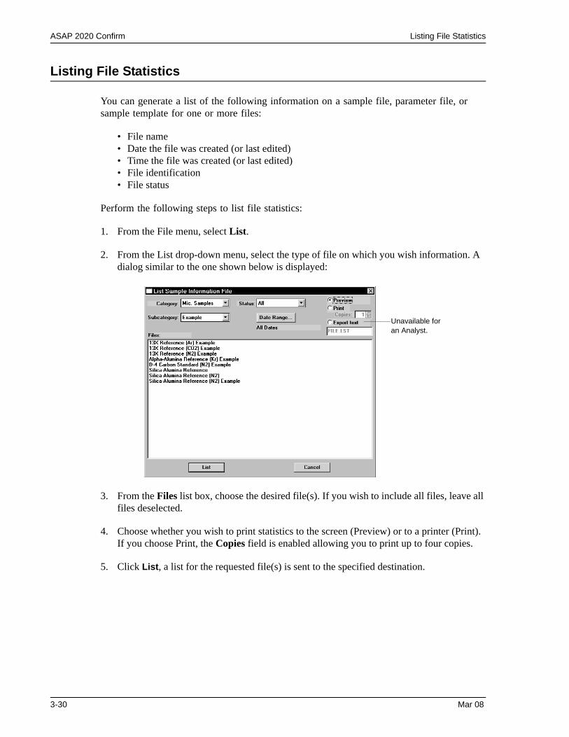
ASAP 2020 Confirm Listing File Statistics
Listing File Statistics
You can generate a list of the following information on a sample file, parameter file, or sample template for one or more files:
• File name• Date the file was created (or last edited)• Time the file was created (or last edited)• File identification• File status
Perform the following steps to list file statistics:
1. From the File menu, select List.
2. From the List drop-down menu, select the type of file on which you wish information. A dialog similar to the one shown below is displayed:
3. From the Files list box, choose the desired file(s). If you wish to include all files, leave all files deselected.
4. Choose whether you wish to print statistics to the screen (Preview) or to a printer (Print). If you choose Print, the Copies field is enabled allowing you to print up to four copies.
5. Click List, a list for the requested file(s) is sent to the specified destination.
Unavailable for an Analyst.
3-30 Mar 08
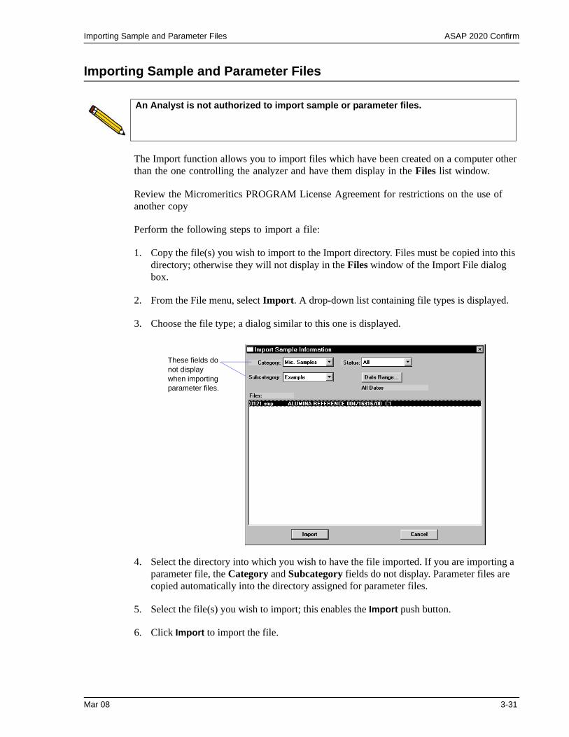
Importing Sample and Parameter Files ASAP 2020 Confirm
Importing Sample and Parameter Files
The Import function allows you to import files which have been created on a computer other than the one controlling the analyzer and have them display in the Files list window.
Review the Micromeritics PROGRAM License Agreement for restrictions on the use of another copy
Perform the following steps to import a file:
1. Copy the file(s) you wish to import to the Import directory. Files must be copied into this directory; otherwise they will not display in the Files window of the Import File dialog box.
2. From the File menu, select Import. A drop-down list containing file types is displayed.
3. Choose the file type; a dialog similar to this one is displayed.
4. Select the directory into which you wish to have the file imported. If you are importing a parameter file, the Category and Subcategory fields do not display. Parameter files are copied automatically into the directory assigned for parameter files.
5. Select the file(s) you wish to import; this enables the Import push button.
6. Click Import to import the file.
An Analyst is not authorized to import sample or parameter files.
These fields do not display when importing parameter files.
Mar 08 3-31
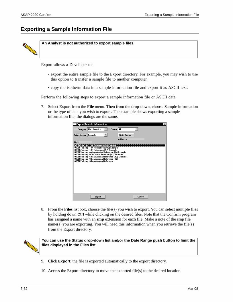
ASAP 2020 Confirm Exporting a Sample Information File
Exporting a Sample Information File
Export allows a Developer to:
• export the entire sample file to the Export directory. For example, you may wish to use this option to transfer a sample file to another computer.
• copy the isotherm data in a sample information file and export it as ASCII text.
Perform the following steps to export a sample information file or ASCII data:
7. Select Export from the File menu. Then from the drop-down, choose Sample information or the type of data you wish to export. This example shows exporting a sample information file; the dialogs are the same.
8. From the Files list box, choose the file(s) you wish to export. You can select multiple files by holding down Ctrl while clicking on the desired files. Note that the Confirm program has assigned a name with an smp extension for each file. Make a note of the smp file name(s) you are exporting. You will need this information when you retrieve the file(s) from the Export directory.
9. Click Export; the file is exported automatically to the export directory.
10. Access the Export directory to move the exported file(s) to the desired location.
An Analyst is not authorized to export sample files.
You can use the Status drop-down list and/or the Date Range push button to limit the files displayed in the Files list.
3-32 Mar 08
Generating Graph Overlays ASAP 2020 Confirm
Generating Graph Overlays
Use graph overlays when you wish to compare graphically results for multiple samples or multiple graphs for one sample. Graphical lines are differentiated by the use of varying symbols and reported in a legend on the report. If color output capability is available, different colors are used instead of symbols.
Graph overlays can be implemented in two ways:
• Multiple Sample Overlays Overlay results for up to eight samples on top of a previously selected sample.
• Multiple Graph OverlaysOverlay two different types of graphs from one sample. The multiple graph overlay capability exists for:
BJH Adsorption/DesorptionDFT Pore Size/Surface EnergyDollimore-Heal Adsorption/DesorptionHorvath-Kawazoe*MP-Method
*Available only if the micropore option is installed.
An Analyst must click Advanced to access the Report Options tab in order to perform these procedures.
Mar 08 3-33
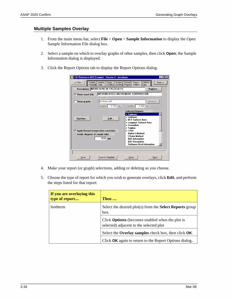
ASAP 2020 Confirm Generating Graph Overlays
Multiple Samples Overlay
1. From the main menu bar, select File > Open > Sample Information to display the Open Sample Information File dialog box.
2. Select a sample on which to overlay graphs of other samples, then click Open; the Sample Information dialog is displayed.
3. Click the Report Options tab to display the Report Options dialog.
4. Make your report (or graph) selections, adding or deleting as you choose.
5. Choose the type of report for which you wish to generate overlays, click Edit, and perform the steps listed for that report:
If you are overlaying this type of report.... Then ....
Isotherm Select the desired plot(s) from the Select Reports group box.
Click Options (becomes enabled when the plot is selected) adjacent to the selected plot
Select the Overlay samples check box, then click OK.
Click OK again to return to the Report Options dialog..
3-34 Mar 08
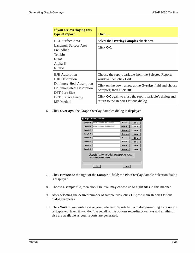
Generating Graph Overlays ASAP 2020 Confirm
6. Click Overlays; the Graph Overlay Samples dialog is displayed.
7. Click Browse to the right of the Sample 1 field; the Plot Overlay Sample Selection dialog is displayed.
8. Choose a sample file, then click OK. You may choose up to eight files in this manner.
9. After selecting the desired number of sample files, click OK; the main Report Options dialog reappears.
10. Click Save if you wish to save your Selected Reports list; a dialog prompting for a reason is displayed. Even if you don’t save, all of the options regarding overlays and anything else are available as your reports are generated.
If you are overlaying this type of report.... Then ....
BET Surface AreaLangmuir Surface AreaFreundlichTemkint-PlotAlpha-Sf-Ratio
Select the Overlay Samples check box.
Click OK.
BJH AdsorptionBJH DesorptionDollimore-Heal AdsorptionDollimore-Heal DesorptionDFT Pore SizeDFT Surface EnergyMP-Method
Choose the report variable from the Selected Reports window, then click Edit.
Click on the down arrow at the Overlay field and choose Samples; then click OK.
Click OK again to close the report variable’s dialog and return to the Report Options dialog.
Mar 08 3-35
ASAP 2020 Confirm Generating Graph Overlays
11. Select Reports >Start Report; the Start Report dialog is displayed with the name of your primary file highlighted.
12. Click Report; one of the following occurs:
• if you clicked Save to save specified overlay options, the Select Reports dialog is displayed.
• If you did not click Save, a dialog stating that a preview report will be generated or you can cancel the operation is displayed. If you choose to generate the preview report, the Select Reports dialog is displayed.
13. Ensure that the desired graph is selected (preceded with a check mark, then click OK.
3-36 Mar 08
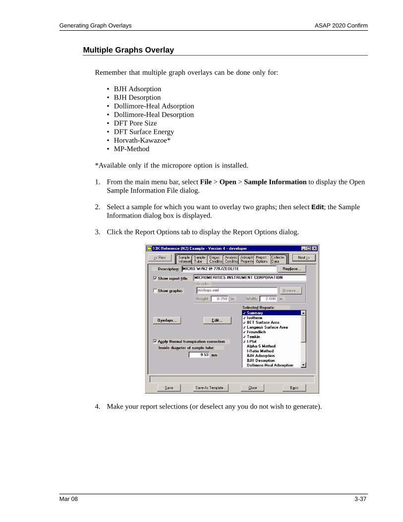
Generating Graph Overlays ASAP 2020 Confirm
Multiple Graphs Overlay
Remember that multiple graph overlays can be done only for:
• BJH Adsorption• BJH Desorption• Dollimore-Heal Adsorption• Dollimore-Heal Desorption• DFT Pore Size• DFT Surface Energy • Horvath-Kawazoe* • MP-Method
*Available only if the micropore option is installed.
1. From the main menu bar, select File > Open > Sample Information to display the Open Sample Information File dialog.
2. Select a sample for which you want to overlay two graphs; then select Edit; the Sample Information dialog box is displayed.
3. Click the Report Options tab to display the Report Options dialog.
4. Make your report selections (or deselect any you do not wish to generate).
Mar 08 3-37
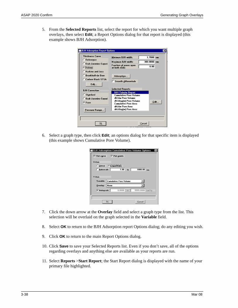
ASAP 2020 Confirm Generating Graph Overlays
5. From the Selected Reports list, select the report for which you want multiple graph overlays, then select Edit; a Report Options dialog for that report is displayed (this example shows BJH Adsorption).
6. Select a graph type, then click Edit; an options dialog for that specific item is displayed (this example shows Cumulative Pore Volume).
7. Click the down arrow at the Overlay field and select a graph type from the list. This selection will be overlaid on the graph selected in the Variable field.
8. Select OK to return to the BJH Adsorption report Options dialog; do any editing you wish.
9. Click OK to return to the main Report Options dialog.
10. Click Save to save your Selected Reports list. Even if you don’t save, all of the options regarding overlays and anything else are available as your reports are run.
11. Select Reports >Start Report; the Start Report dialog is displayed with the name of your primary file highlighted.
3-38 Mar 08
Generating Graph Overlays ASAP 2020 Confirm
12. Click Report; one of the following occurs:
• if you clicked Save to save specified overlay options, the Select Reports dialog is displayed.
• If you did not click Save, a dialog stating that a preview report will be generated or you can cancel the operation is displayed. If you choose to generate the preview report, the Select Reports dialog is displayed.
13. Ensure that the desired graph is selected (preceded with a check mark, then click OK.
Mar 08 3-39

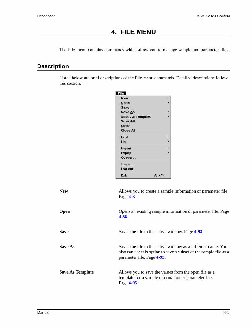
Description ASAP 2020 Confirm
4. FILE MENU
The File menu contains commands which allow you to manage sample and parameter files.
Description
Listed below are brief descriptions of the File menu commands. Detailed descriptions follow this section.
New Allows you to create a sample information or parameter file. Page 4-3.
Open Opens an existing sample information or parameter file. Page 4-88.
Save Saves the file in the active window. Page 4-93.
Save As Saves the file in the active window as a different name. You also can use this option to save a subset of the sample file as a parameter file. Page 4-93.
Save As Template Allows you to save the values from the open file as a template for a sample information or parameter file. Page 4-95.
Mar 08 4-1
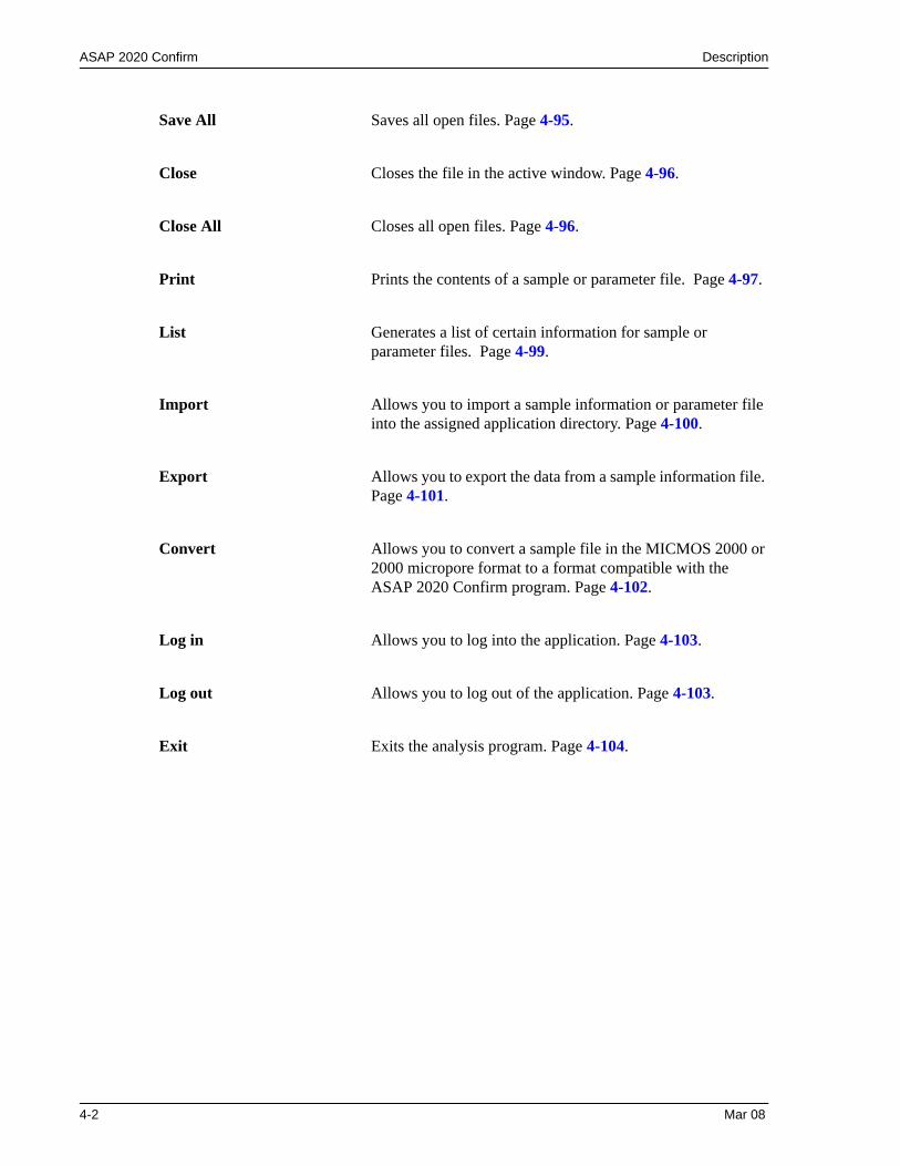
ASAP 2020 Confirm Description
Save All Saves all open files. Page 4-95.
Close Closes the file in the active window. Page 4-96.
Close All Closes all open files. Page 4-96.
Print Prints the contents of a sample or parameter file. Page 4-97.
List Generates a list of certain information for sample or parameter files. Page 4-99.
Import Allows you to import a sample information or parameter file into the assigned application directory. Page 4-100.
Export Allows you to export the data from a sample information file. Page 4-101.
Convert Allows you to convert a sample file in the MICMOS 2000 or 2000 micropore format to a format compatible with the ASAP 2020 Confirm program. Page 4-102.
Log in Allows you to log into the application. Page 4-103.
Log out Allows you to log out of the application. Page 4-103.
Exit Exits the analysis program. Page 4-104.
4-2 Mar 08
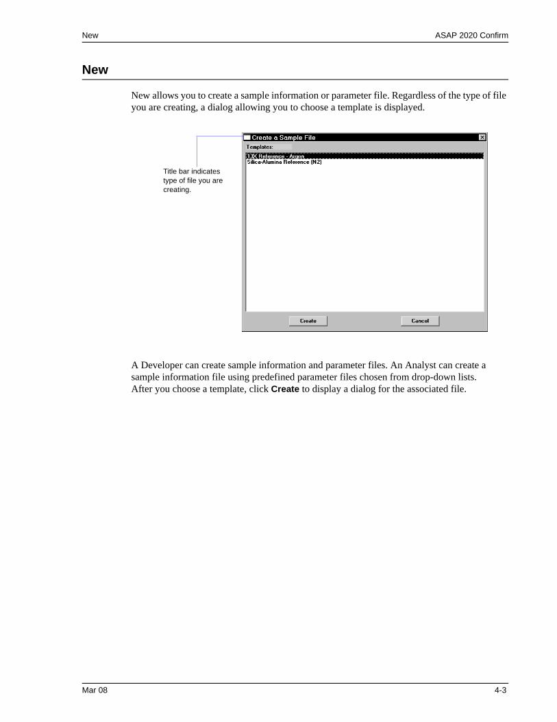
New ASAP 2020 Confirm
New
New allows you to create a sample information or parameter file. Regardless of the type of file you are creating, a dialog allowing you to choose a template is displayed.
A Developer can create sample information and parameter files. An Analyst can create a sample information file using predefined parameter files chosen from drop-down lists.After you choose a template, click Create to display a dialog for the associated file.
Title bar indicates type of file you are creating.
Mar 08 4-3
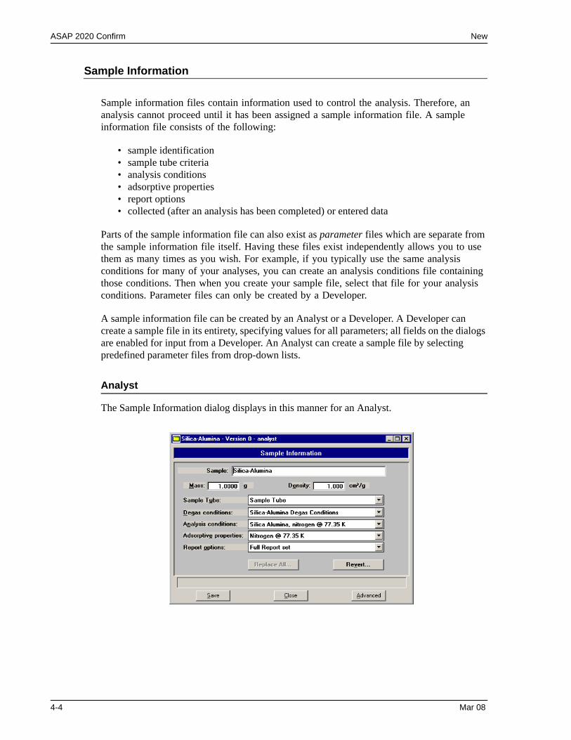
ASAP 2020 Confirm New
Sample Information
Sample information files contain information used to control the analysis. Therefore, an analysis cannot proceed until it has been assigned a sample information file. A sample information file consists of the following:
• sample identification• sample tube criteria• analysis conditions• adsorptive properties• report options• collected (after an analysis has been completed) or entered data
Parts of the sample information file can also exist as parameter files which are separate from the sample information file itself. Having these files exist independently allows you to use them as many times as you wish. For example, if you typically use the same analysis conditions for many of your analyses, you can create an analysis conditions file containing those conditions. Then when you create your sample file, select that file for your analysis conditions. Parameter files can only be created by a Developer.
A sample information file can be created by an Analyst or a Developer. A Developer can create a sample file in its entirety, specifying values for all parameters; all fields on the dialogs are enabled for input from a Developer. An Analyst can create a sample file by selecting predefined parameter files from drop-down lists.
Analyst
The Sample Information dialog displays in this manner for an Analyst.
4-4 Mar 08
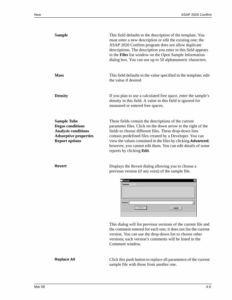
New ASAP 2020 Confirm
Sample This field defaults to the description of the template. You must enter a new description or edit the existing one; the ASAP 2020 Confirm program does not allow duplicate descriptions. The description you enter in this field appears in the Files list window on the Open Sample Information dialog box. You can use up to 50 alphanumeric characters.
Mass This field defaults to the value specified in the template; edit the value if desired
Density If you plan to use a calculated free space, enter the sample’s density in this field. A value in this field is ignored for measured or entered free spaces.
Sample TubeDegas conditionsAnalysis conditionsAdsorptive propertiesReport options
These fields contain the descriptions of the current parameter files. Click on the down arrow to the right of the fields to choose different files. These drop-down lists contain predefined files created by a Developer. You can view the values contained in the files by clicking Advanced; however, you cannot edit them. You can edit details of some reports by clicking Edit.
Revert Displays the Revert dialog allowing you to choose a previous version (if any exist) of the sample file.
This dialog will list previous versions of the current file and the comment entered for each one; it does not list the current version. You can use the drop-down list to choose other versions; each version’s comments will be listed in the Comment window.
Replace All Click this push button to replace all parameters of the current sample file with those from another one.
Mar 08 4-5
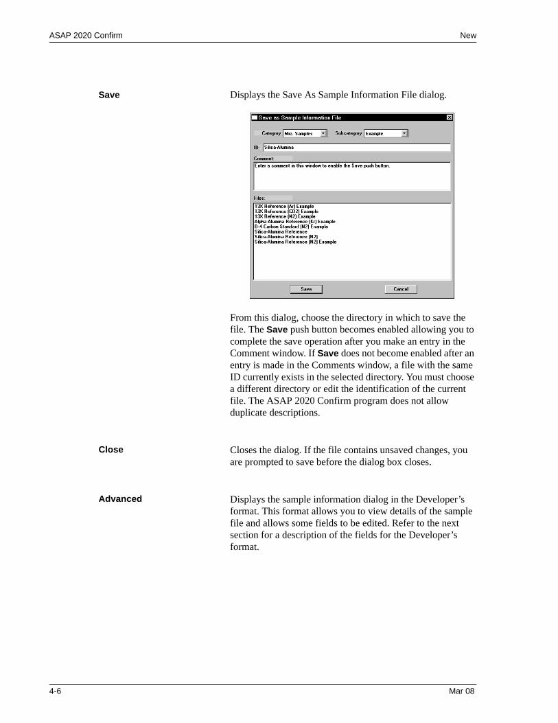
ASAP 2020 Confirm New
Save Displays the Save As Sample Information File dialog.
From this dialog, choose the directory in which to save the file. The Save push button becomes enabled allowing you to complete the save operation after you make an entry in the Comment window. If Save does not become enabled after an entry is made in the Comments window, a file with the same ID currently exists in the selected directory. You must choose a different directory or edit the identification of the current file. The ASAP 2020 Confirm program does not allow duplicate descriptions.
Close Closes the dialog. If the file contains unsaved changes, you are prompted to save before the dialog box closes.
Advanced Displays the sample information dialog in the Developer’s format. This format allows you to view details of the sample file and allows some fields to be edited. Refer to the next section for a description of the fields for the Developer’s format.
4-6 Mar 08
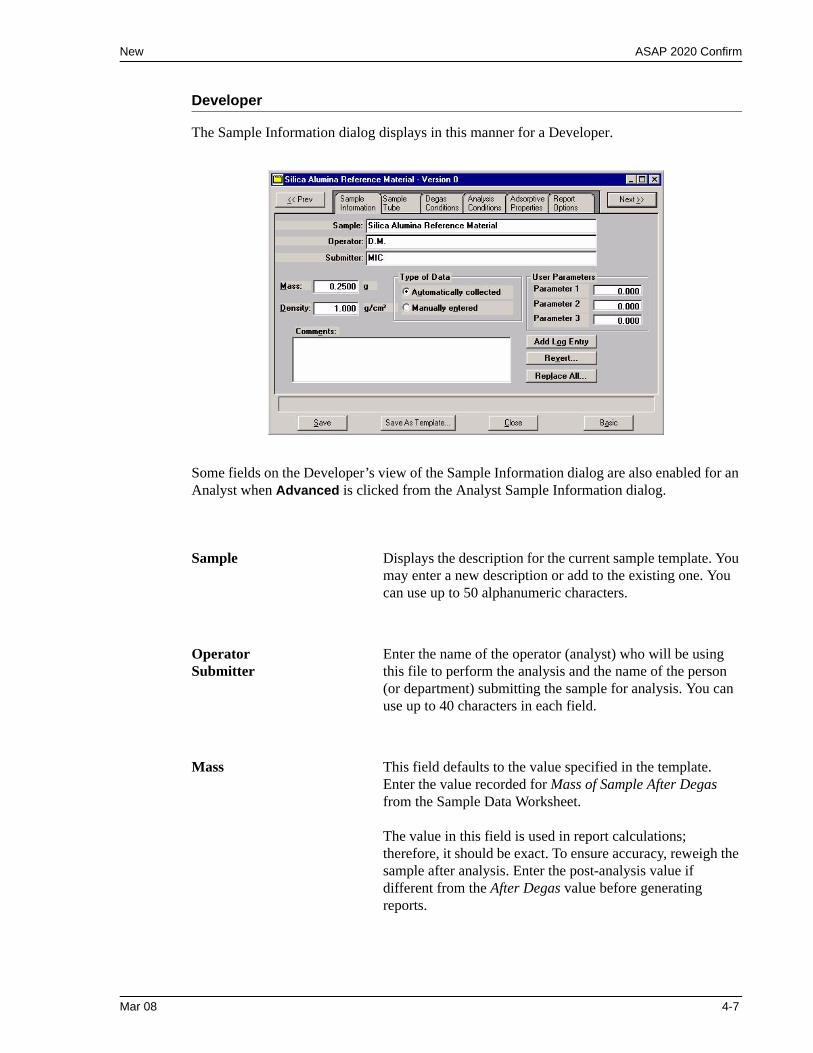
New ASAP 2020 Confirm
Developer
The Sample Information dialog displays in this manner for a Developer.
Some fields on the Developer’s view of the Sample Information dialog are also enabled for an Analyst when Advanced is clicked from the Analyst Sample Information dialog.
Sample Displays the description for the current sample template. You may enter a new description or add to the existing one. You can use up to 50 alphanumeric characters.
Operator Submitter
Enter the name of the operator (analyst) who will be using this file to perform the analysis and the name of the person (or department) submitting the sample for analysis. You can use up to 40 characters in each field.
Mass This field defaults to the value specified in the template. Enter the value recorded for Mass of Sample After Degas from the Sample Data Worksheet.
The value in this field is used in report calculations; therefore, it should be exact. To ensure accuracy, reweigh the sample after analysis. Enter the post-analysis value if different from the After Degas value before generating reports.
Mar 08 4-7
ASAP 2020 Confirm New
Density If you plan to use a calculated free space, enter the sample’s density in this field. A value in this field is ignored for measured or entered free spaces.
Type of Data Choose whether you wish to enter the data or have it collected automatically by the analysis program. If you choose Manually entered, an “Entered” tab is added so that you may enter the desired data. You cannot enter data if you are creating the file on a computer that is not attached to the analyzer.
User Parameters These fields are used primarily for SPC (Statistical Process Control) reporting. However, they can be used for other data as well. You may wish to enter specific analysis conditions or sample criteria. These parameters print on the Options report. Select Options > Edit Labels to specify the param-eters you wish to report. The parameter(s) you specify replace the User Parameter label(s).
If desired, you can have these fields omitted from the sample information file (refer to Edit Labels, page 7-3).
Comments Allows you to enter comments about the sample or its analysis conditions. Anything you enter in this window is printed in the header of the report.
Replace All Click this push button to replace all parameters of the current sample file with those from another one.
4-8 Mar 08
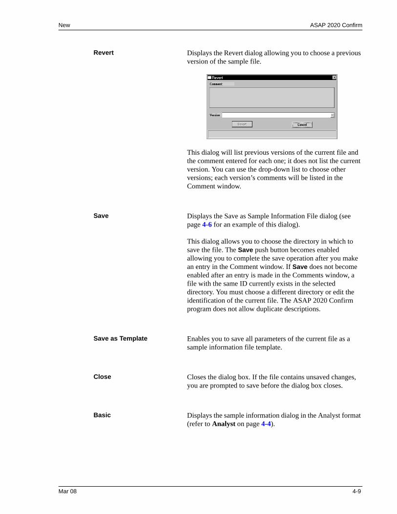
New ASAP 2020 Confirm
Revert Displays the Revert dialog allowing you to choose a previous version of the sample file.
This dialog will list previous versions of the current file and the comment entered for each one; it does not list the current version. You can use the drop-down list to choose other versions; each version’s comments will be listed in the Comment window.
Save Displays the Save as Sample Information File dialog (see page 4-6 for an example of this dialog).
This dialog allows you to choose the directory in which to save the file. The Save push button becomes enabled allowing you to complete the save operation after you make an entry in the Comment window. If Save does not become enabled after an entry is made in the Comments window, a file with the same ID currently exists in the selected directory. You must choose a different directory or edit the identification of the current file. The ASAP 2020 Confirm program does not allow duplicate descriptions.
Save as Template Enables you to save all parameters of the current file as a sample information file template.
Close Closes the dialog box. If the file contains unsaved changes, you are prompted to save before the dialog box closes.
Basic Displays the sample information dialog in the Analyst format (refer to Analyst on page 4-4).
Mar 08 4-9
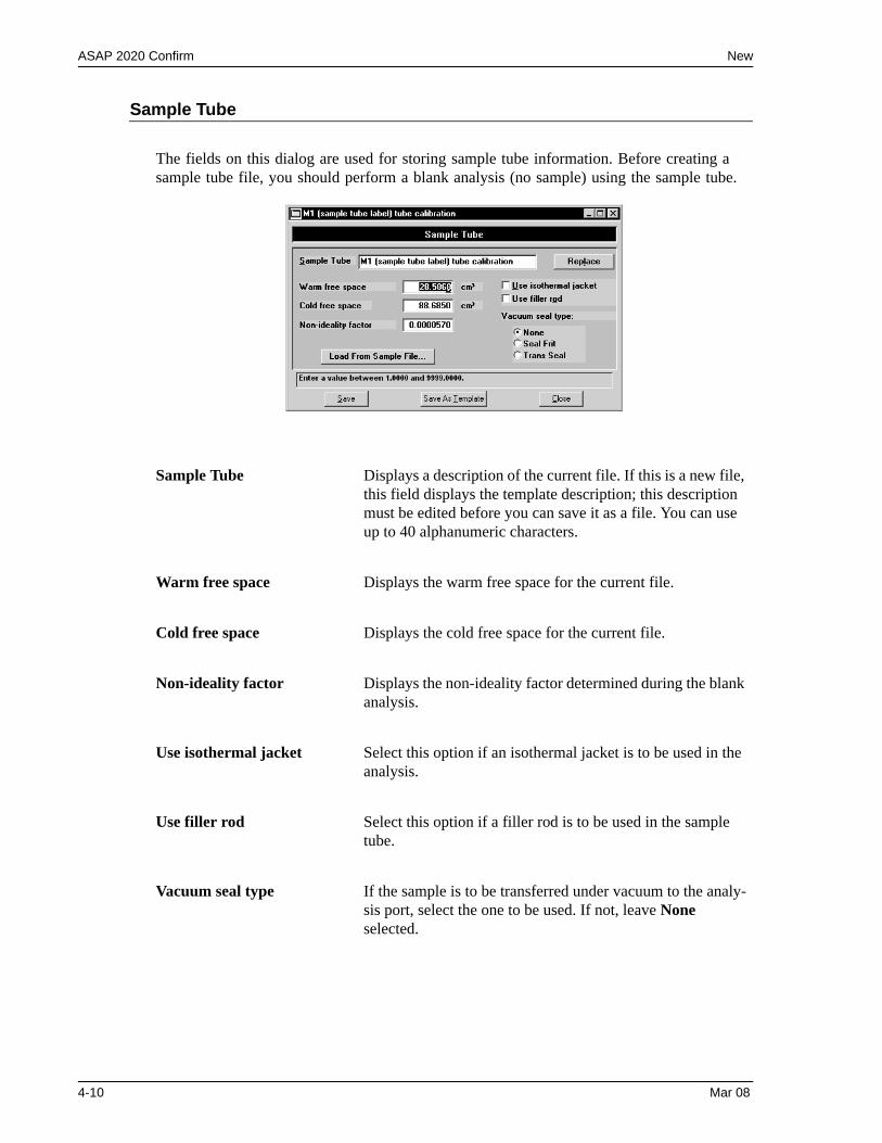
ASAP 2020 Confirm New
Sample Tube
The fields on this dialog are used for storing sample tube information. Before creating a sample tube file, you should perform a blank analysis (no sample) using the sample tube.
Sample Tube Displays a description of the current file. If this is a new file, this field displays the template description; this description must be edited before you can save it as a file. You can use up to 40 alphanumeric characters.
Warm free space Displays the warm free space for the current file.
Cold free space Displays the cold free space for the current file.
Non-ideality factor Displays the non-ideality factor determined during the blank analysis.
Use isothermal jacket Select this option if an isothermal jacket is to be used in the analysis.
Use filler rod Select this option if a filler rod is to be used in the sample tube.
Vacuum seal type If the sample is to be transferred under vacuum to the analy-sis port, select the one to be used. If not, leave None selected.
4-10 Mar 08
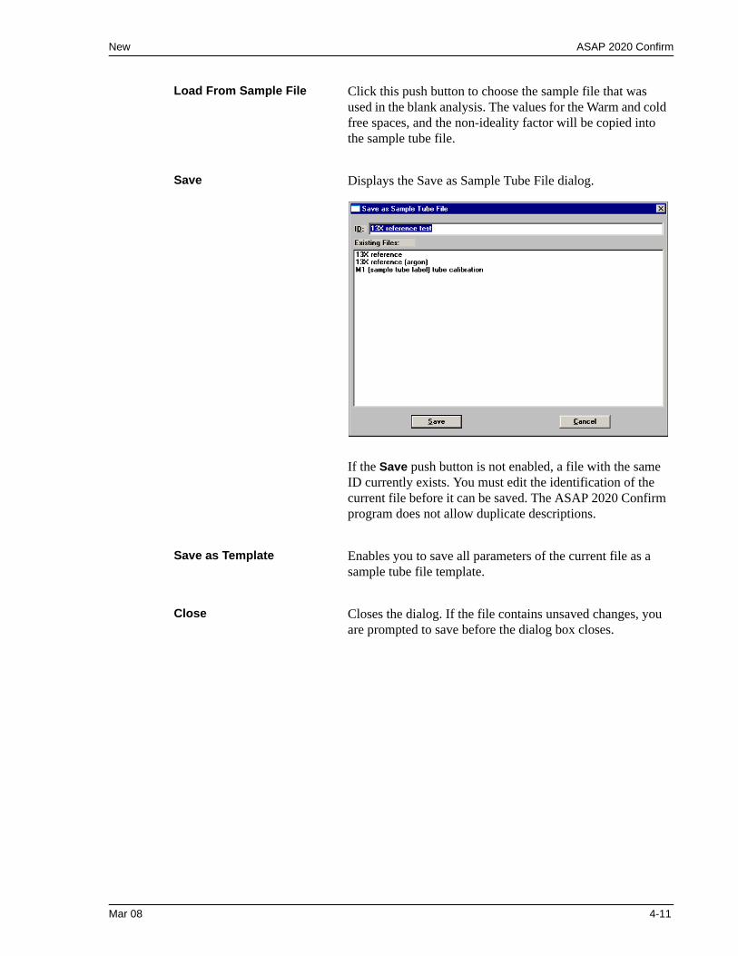
New ASAP 2020 Confirm
Load From Sample File Click this push button to choose the sample file that was used in the blank analysis. The values for the Warm and cold free spaces, and the non-ideality factor will be copied into the sample tube file.
Save Displays the Save as Sample Tube File dialog.
If the Save push button is not enabled, a file with the same ID currently exists. You must edit the identification of the current file before it can be saved. The ASAP 2020 Confirm program does not allow duplicate descriptions.
Save as Template Enables you to save all parameters of the current file as a sample tube file template.
Close Closes the dialog. If the file contains unsaved changes, you are prompted to save before the dialog box closes.
Mar 08 4-11
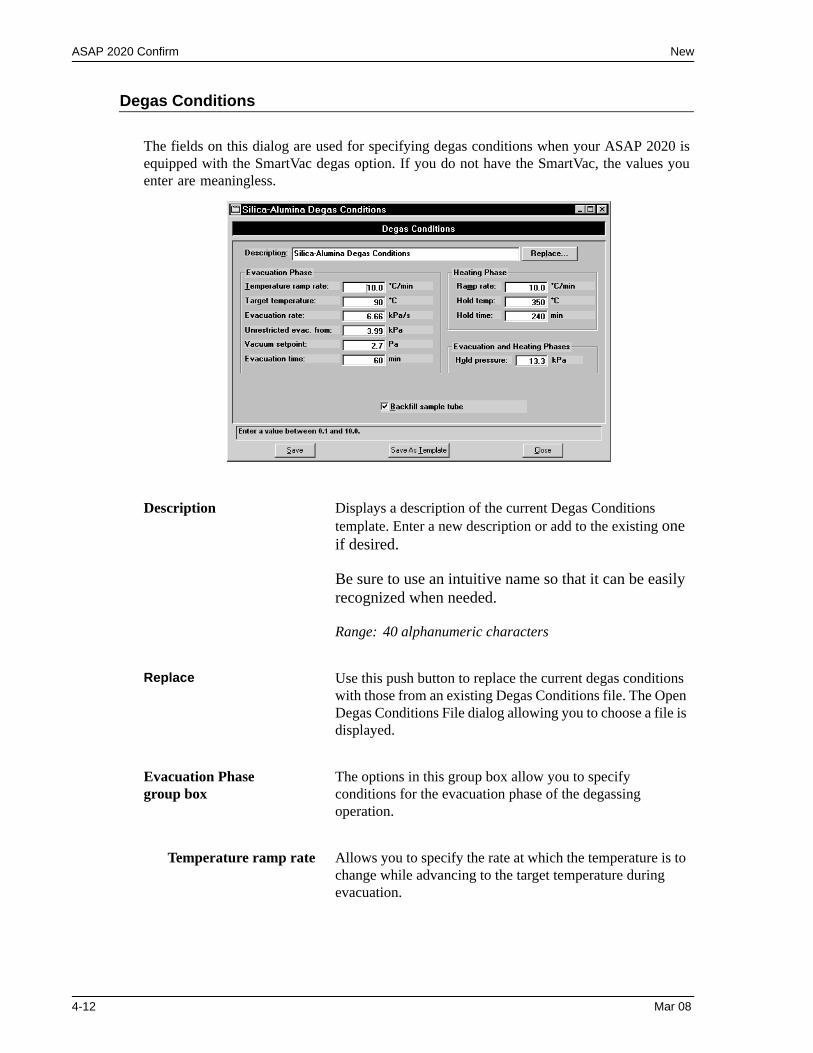
ASAP 2020 Confirm New
Degas Conditions
The fields on this dialog are used for specifying degas conditions when your ASAP 2020 is equipped with the SmartVac degas option. If you do not have the SmartVac, the values you enter are meaningless.
Description Displays a description of the current Degas Conditions template. Enter a new description or add to the existing one if desired.
Be sure to use an intuitive name so that it can be easily recognized when needed.
Range: 40 alphanumeric characters
Replace Use this push button to replace the current degas conditions with those from an existing Degas Conditions file. The Open Degas Conditions File dialog allowing you to choose a file is displayed.
Evacuation Phasegroup box
The options in this group box allow you to specify conditions for the evacuation phase of the degassing operation.
Temperature ramp rate Allows you to specify the rate at which the temperature is to change while advancing to the target temperature during evacuation.
4-12 Mar 08
New ASAP 2020 Confirm
Target temperature Allows you to specify a temperature at which the sample will be held for the remainder of the evacuation.
Evacuation rate Enables you to specify an evacuation rate for initial evacuation.
Unrestricted evac. from Enables you to specify a pressure at which unrestricted sample evacuation will begin.
Vacuum setpoint Enables you to specify the vacuum level to be achieved before evacuation begins.
Evacuation time Enables yo to specify how long the sample is to be evacuated prior to the second stage of heating.
Heating Phasegroup box
The options in this group box allow you to specify conditions for the heating phase of the degassing operation.
Ramp rate Enables you to specify the rate at which the temperature will change after evacuation while advancing to the hold temperature.
Hold temp Enables you to specify a temperature at which the sample is to be held during degassing.
Hold time Enables you to specify how long the sample is to be held at the specified temperature before beginning to cool down.
Hold Pressure If during the temperature ramp the pressure exceeds the value you enter in this field, the ramp will be suspended until the pressure returns to a safe level.
Backfill Sample Tube Select this option to have the sample tube backfilled. You should deselect this option if you are using the TranSeal; this allows the sample to remain under vacuum while transferring to the analysis port.
Mar 08 4-13
ASAP 2020 Confirm New
Save Displays the Save as Degas Conditions File dialog (see page 4-11 for an example of this dialog).
If the Save push button is not enabled, a file with the same ID currently exists. You must edit the identification of the current file before it can be saved. The ASAP 2020 Confirm program does not allow duplicate descriptions.
Save as Template Enables you to save the parameters of the current file as a Degas Conditions file template.
Close Closes the dialog box. If the file contains unsaved changes, you are prompted to save before the dialog box closes.
4-14 Mar 08
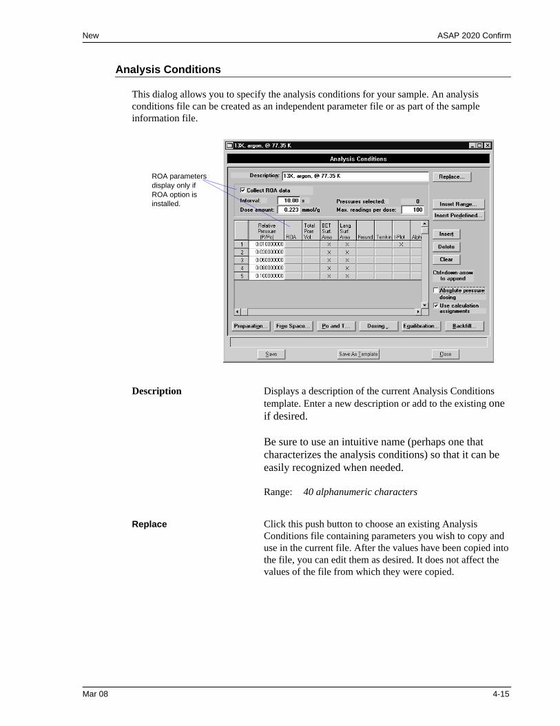
New ASAP 2020 Confirm
Analysis Conditions
This dialog allows you to specify the analysis conditions for your sample. An analysis conditions file can be created as an independent parameter file or as part of the sample information file.
Description Displays a description of the current Analysis Conditions template. Enter a new description or add to the existing one if desired.
Be sure to use an intuitive name (perhaps one that characterizes the analysis conditions) so that it can be easily recognized when needed.
Range: 40 alphanumeric characters
Replace Click this push button to choose an existing Analysis Conditions file containing parameters you wish to copy and use in the current file. After the values have been copied into the file, you can edit them as desired. It does not affect the values of the file from which they were copied.
ROA parameters display only if ROA option is installed.
Mar 08 4-15
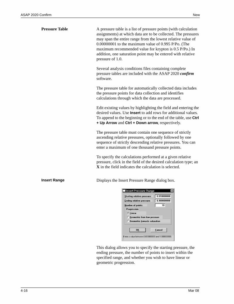
ASAP 2020 Confirm New
Pressure Table A pressure table is a list of pressure points (with calculation assignments) at which data are to be collected. The pressures may span the entire range from the lowest relative value of 0.00000001 to the maximum value of 0.995 P/Po. (The maximum recommended value for krypton is 0.5 P/Po.) In addition, one saturation point may be entered with relative pressure of 1.0.
Several analysis conditions files containing complete pressure tables are included with the ASAP 2020 confirm software.
The pressure table for automatically collected data includes the pressure points for data collection and identifies calculations through which the data are processed.
Edit existing values by highlighting the field and entering the desired values. Use Insert to add rows for additional values. To append to the beginning or to the end of the table, use Ctrl + Up Arrow and Ctrl + Down arrow, respectively.
The pressure table must contain one sequence of strictly ascending relative pressures, optionally followed by one sequence of strictly descending relative pressures. You can enter a maximum of one thousand pressure points.
To specify the calculations performed at a given relative pressure, click in the field of the desired calculation type; an X in the field indicates the calculation is selected.
Insert Range Displays the Insert Pressure Range dialog box.
This dialog allows you to specify the starting pressure, the ending pressure, the number of points to insert within the specified range, and whether you wish to have linear or geometric progression.
4-16 Mar 08
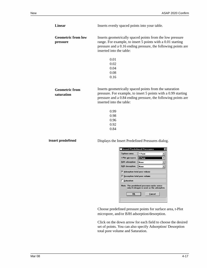
New ASAP 2020 Confirm
Linear Inserts evenly spaced points into your table.
Geometric from low pressure
Inserts geometrically spaced points from the low pressure range. For example, to insert 5 points with a 0.01 starting pressure and a 0.16 ending pressure, the following points are inserted into the table:
0.010.020.040.080.16
Geometric from saturation
Inserts geometrically spaced points from the saturation pressure. For example, to insert 5 points with a 0.99 starting pressure and a 0.84 ending pressure, the following points are inserted into the table:
0.990.980.960.920.84
Insert predefined Displays the Insert Predefined Pressures dialog.
Choose predefined pressure points for surface area, t-Plot micropore, and/or BJH adsorption/desorption.
Click on the down arrow for each field to choose the desired set of points. You can also specify Adsorption/ Desorption total pore volume and Saturation.
Mar 08 4-17
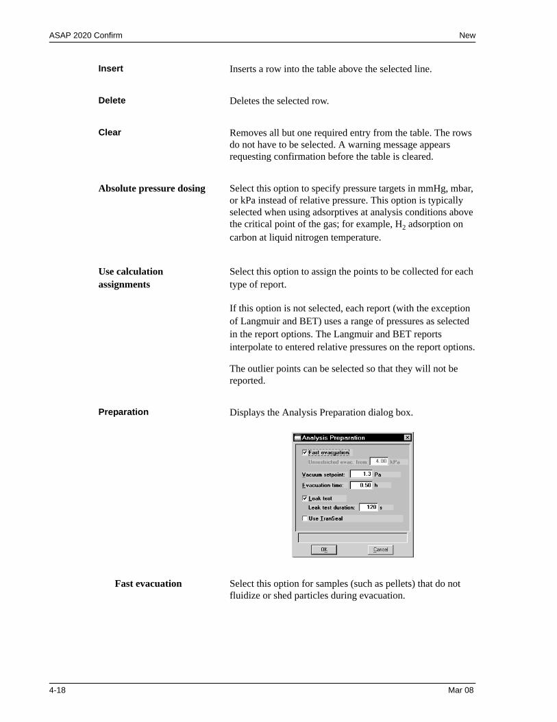
ASAP 2020 Confirm New
Insert Inserts a row into the table above the selected line.
Delete Deletes the selected row.
Clear Removes all but one required entry from the table. The rows do not have to be selected. A warning message appears requesting confirmation before the table is cleared.
Absolute pressure dosing Select this option to specify pressure targets in mmHg, mbar, or kPa instead of relative pressure. This option is typically selected when using adsorptives at analysis conditions above the critical point of the gas; for example, H2 adsorption on carbon at liquid nitrogen temperature.
Use calculationassignments
Select this option to assign the points to be collected for each type of report.
If this option is not selected, each report (with the exception of Langmuir and BET) uses a range of pressures as selected in the report options. The Langmuir and BET reports interpolate to entered relative pressures on the report options.
The outlier points can be selected so that they will not be reported.
Preparation Displays the Analysis Preparation dialog box.
Fast evacuation Select this option for samples (such as pellets) that do not fluidize or shed particles during evacuation.
4-18 Mar 08
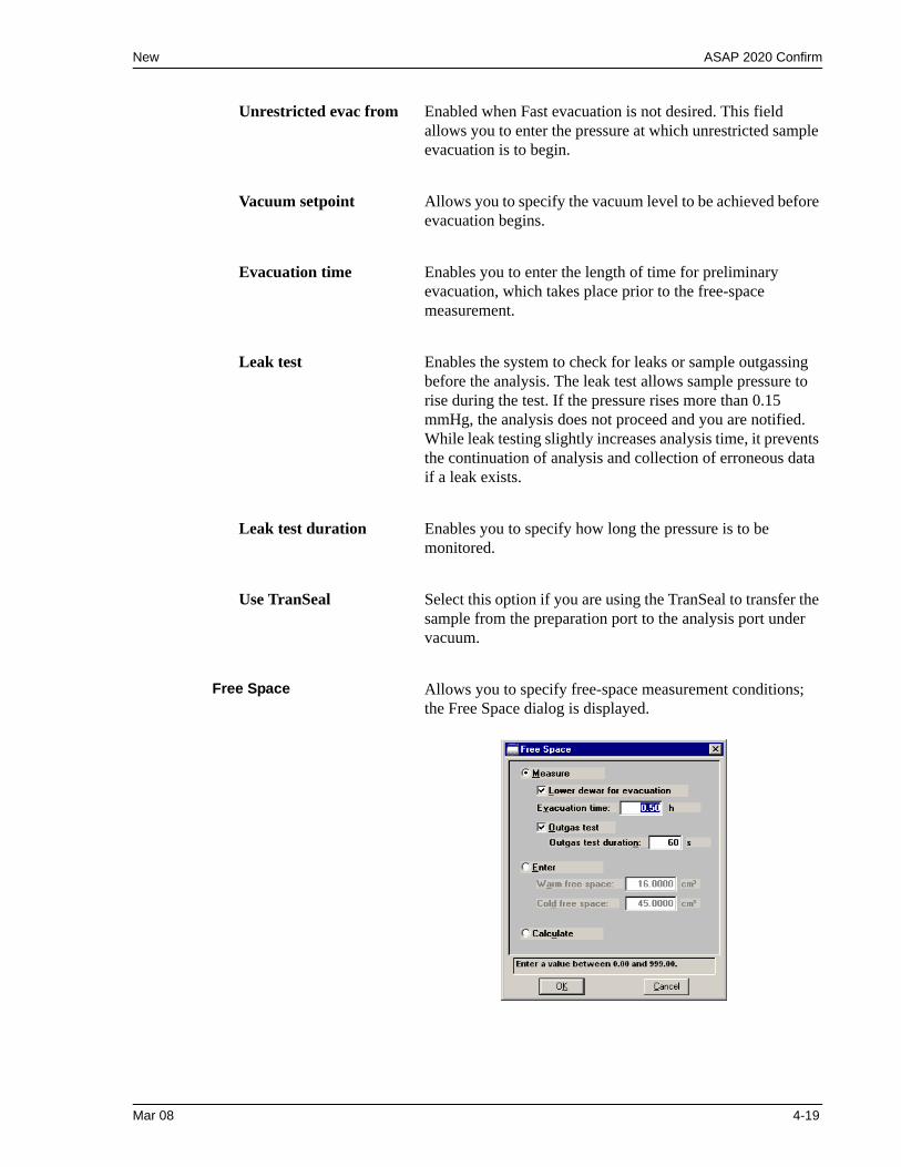
New ASAP 2020 Confirm
Unrestricted evac from Enabled when Fast evacuation is not desired. This field allows you to enter the pressure at which unrestricted sample evacuation is to begin.
Vacuum setpoint Allows you to specify the vacuum level to be achieved before evacuation begins.
Evacuation time Enables you to enter the length of time for preliminary evacuation, which takes place prior to the free-space measurement.
Leak test Enables the system to check for leaks or sample outgassing before the analysis. The leak test allows sample pressure to rise during the test. If the pressure rises more than 0.15 mmHg, the analysis does not proceed and you are notified. While leak testing slightly increases analysis time, it prevents the continuation of analysis and collection of erroneous data if a leak exists.
Leak test duration Enables you to specify how long the pressure is to be monitored.
Use TranSeal Select this option if you are using the TranSeal to transfer the sample from the preparation port to the analysis port under vacuum.
Free Space Allows you to specify free-space measurement conditions; the Free Space dialog is displayed.
Mar 08 4-19
ASAP 2020 Confirm New
.Measure Select this option to have free space measured automatically
by the system.
Typically, it is best to measure the free space when analyzing macro- and mesoporous samples, and for routine surface area measurements.
Select Lower dewar for evacuation to lower the dewar following free-space measurements.
Evacuation time enables you to specify how long evacuation is to take place following the measured free space
Select Outgas test to check for system leaks or sample outgassing. After free space is measured, the Dewar is lowered and the sample evacuated for 30 minutes. The leak test is performed after evacuation. If a leak is found, the leak test repeats nine times, with 30 minutes evacuation between tests. If the 10th leak check fails, the analysis stops and you are notified. Leak testing slightly increases analysis time, it prevents the continuation of analysis and collection of erroneous data if a leak occurs.
Outgas test duration indicates the number of seconds the leak test is performed.
Enter Select this option to enter values for the warm and cold free spaces. You may need to use this option if the sample retains helium and measurement of very low micron range pressures are required.
If you change the entered free-space value after the preliminary analysis stage is 50% complete, the change does not affect the analysis.
Warm free space is the sample tube gas capacity measured at room temperature.
Cold free space is the sample tube gas capacity measured with the Dewar raised.
4-20 Mar 08
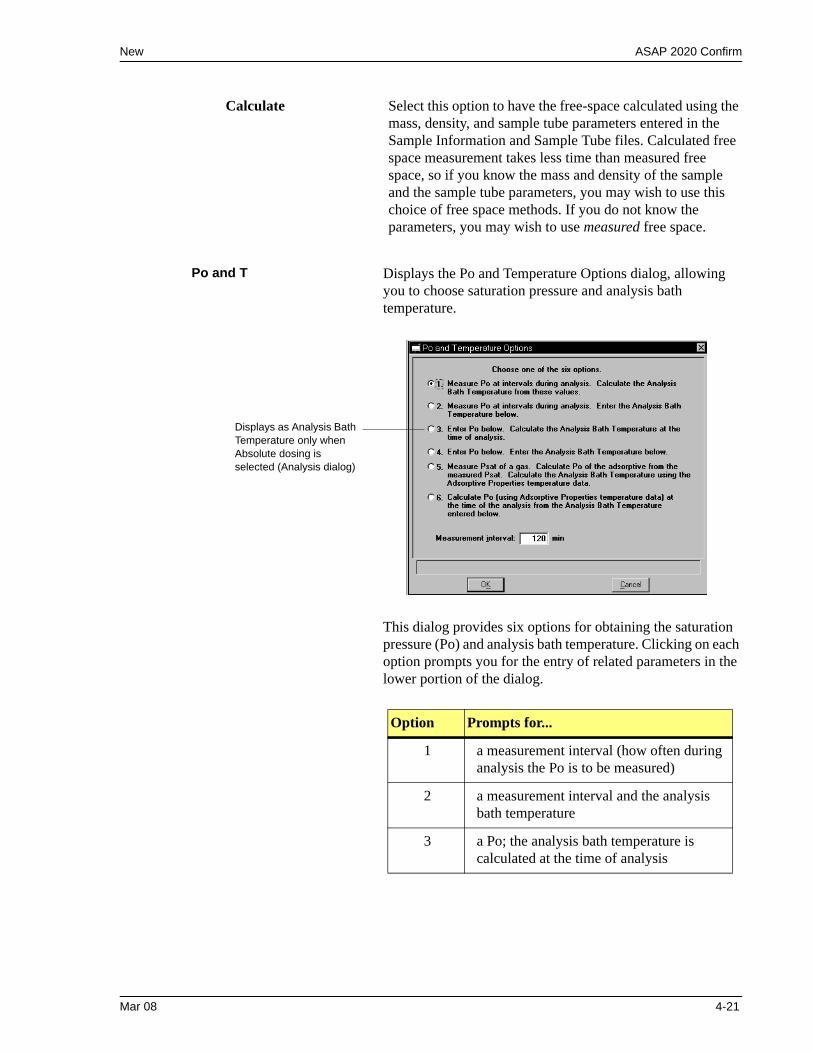
New ASAP 2020 Confirm
Calculate Select this option to have the free-space calculated using the mass, density, and sample tube parameters entered in the Sample Information and Sample Tube files. Calculated free space measurement takes less time than measured free space, so if you know the mass and density of the sample and the sample tube parameters, you may wish to use this choice of free space methods. If you do not know the parameters, you may wish to use measured free space.
Po and T Displays the Po and Temperature Options dialog, allowing you to choose saturation pressure and analysis bath temperature.
This dialog provides six options for obtaining the saturation pressure (Po) and analysis bath temperature. Clicking on each option prompts you for the entry of related parameters in the lower portion of the dialog.
Option Prompts for...
1 a measurement interval (how often during analysis the Po is to be measured)
2 a measurement interval and the analysis bath temperature
3 a Po; the analysis bath temperature is calculated at the time of analysis
Displays as Analysis Bath Temperature only when Absolute dosing is selected (Analysis dialog)
Mar 08 4-21
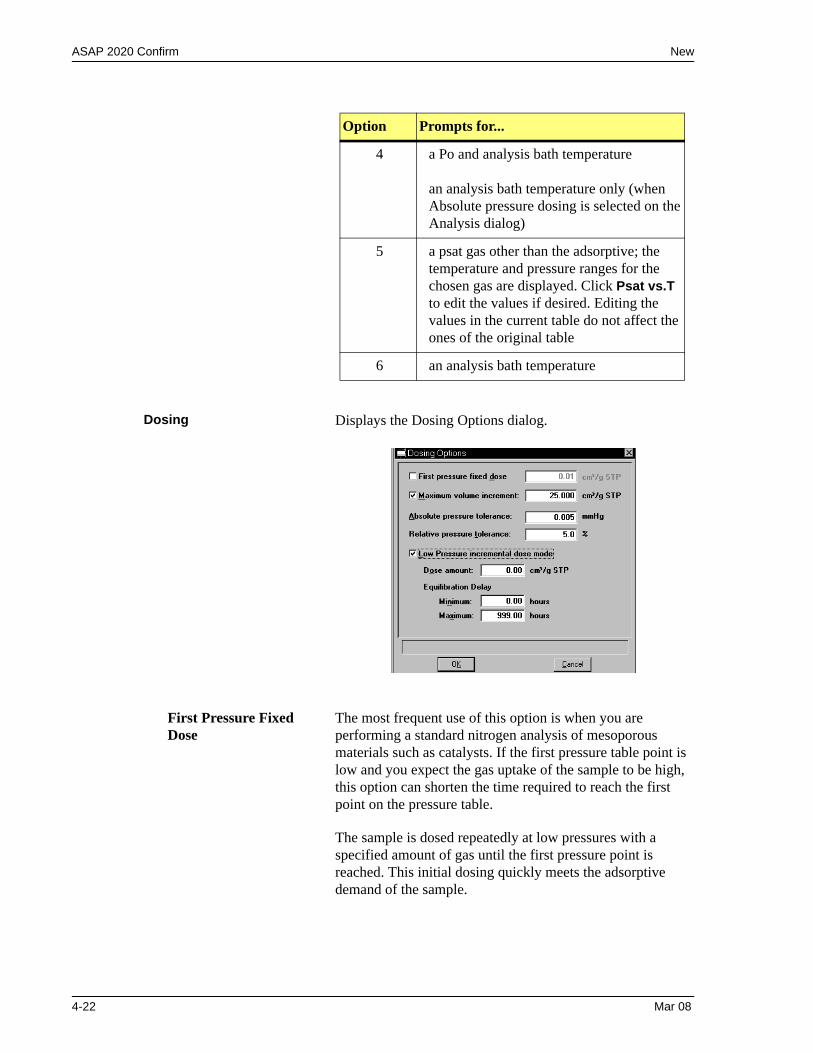
ASAP 2020 Confirm New
Option Prompts for...
4 a Po and analysis bath temperature
an analysis bath temperature only (when Absolute pressure dosing is selected on the Analysis dialog)
5 a psat gas other than the adsorptive; the temperature and pressure ranges for the chosen gas are displayed. Click Psat vs.T to edit the values if desired. Editing the values in the current table do not affect the ones of the original table
6 an analysis bath temperature
Dosing Displays the Dosing Options dialog.
First Pressure Fixed Dose
The most frequent use of this option is when you are performing a standard nitrogen analysis of mesoporous materials such as catalysts. If the first pressure table point is low and you expect the gas uptake of the sample to be high, this option can shorten the time required to reach the first point on the pressure table.
The sample is dosed repeatedly at low pressures with a specified amount of gas until the first pressure point is reached. This initial dosing quickly meets the adsorptive demand of the sample.
4-22 Mar 08
New ASAP 2020 Confirm
First Pressure Fixed Dose(continued)
The first point on the pressure table is the threshold value, triggering the transition from the Fixed Dose Mode to Pressure Table Mode. When the first pressure table value is reached, Fixed Dose Mode is disabled, and points are equilibrated and recorded in accordance with the specified pressure table. In the field adjacent to this option, enter the amount of gas that is to be added to the sample for each dose cycle.
This option is disabled if Low pressure incremental dose mode is selected.
Maximum volume increment
Select this option to determine when additional data points are collected between target pressures in regions of adsorption. When the maximum increment has been adsorbed since the last collected data point, another point is equilibrated and collected.
During desorption, this field is treated as a maximum volume “decrement” value.
Absolute and Relative pressure tolerance
The values entered in these fields are used to determine how close the actual pressure must be to each target pressure from the pressure table. At lower pressures the relative tolerance value is smaller, and at higher pressures the absolute tolerance value is smaller. The lesser (or more stringent) of these two criteria are used to determine the tolerance
For example, with relative tolerance = 5% and absolute tolerance = 5 mmHg, the relative tolerance at 40 mmHg target pressure is 5% of 40 mmHg, or 2 mmHg; 2 mmHg is smaller than the absolute tolerance of 5 mmHg, so 2 mmHg is used. At 200 mmHg target pressure, the relative tolerance is 5% of 200 mmHg, or 10 mmHg; in this case, the absolute tolerance of 5 mmHg is smaller and is used.
In the above example, a minimum pressure of 40 - 2 = 38 mmHg must be attained to collect data for a target pressure of 40 mmHg. For a target of 200 mmHg, 200 - 5 = 195 mmHg must be attained.
Normally, surface area measurement points are widely spaced, and the resulting measurement is not very sensitive to the precise location of points so wider tolerances may be used. Unnecessarily tight tolerances lengthen the analysis.
Mar 08 4-23
ASAP 2020 Confirm New
Low pressure incrementaldose mode
Enabled only if the MicroPore option is installed. Choose this option when you are performing an analysis of microporous materials. At low pressures on Type 1 isotherms, the pressure points are very closely spaced, making a useful pressure table difficult to define. Choosing this mode enables you to measure equilibrium points at approximately equal intervals on the quantity adsorbed axis. Each dose is fully equilibrated and recorded as a data point.
In this mode, the sample is successively dosed with a specified amount of gas until the first pressure point is reached. The first point is the threshold value, triggering the transition from Incremental Dose Mode to Pressure Table Mode. When the first pressure table value is reached, Incremental Dose Mode is disabled, and points are recorded in accordance with the specified pressure table. Because the data points recorded during Incremental Dose Mode may define most of the analysis, one point on the pressure table can be sufficient and serve as the end point for the analysis.
This field is disabled if First Pressure Fixed Dose Mode is selected.
The next three fields are enabled only if Low pressure incremental dose mode is selected
Dose amount Enter the amount of gas to be added to the sample for each data point until the first point on the pressure table is reached.
Equilibration delay MinimumUse this option to prevent premature equilibration caused by reduced percentage sensitivity to pressure changes at the low-est pressures.
MaximumUse this option to prevent the effects of long term tempera-ture or pressure drift, which may cause the instrument to wait an excessive length of time for equilibration.
4-24 Mar 08
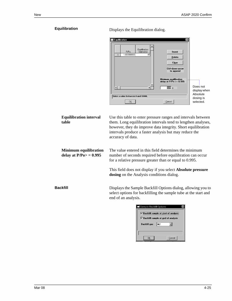
New ASAP 2020 Confirm
Equilibration Displays the Equilibration dialog.
Equilibration interval table
Use this table to enter pressure ranges and intervals between them. Long equilibration intervals tend to lengthen analyses, however, they do improve data integrity. Short equilibration intervals produce a faster analysis but may reduce the accuracy of data.
Minimum equilibration delay at P/Po> = 0.995
The value entered in this field determines the minimum number of seconds required before equilibration can occur for a relative pressure greater than or equal to 0.995.
This field does not display if you select Absolute pressure dosing on the Analysis conditions dialog.
Backfill Displays the Sample Backfill Options dialog, allowing you to select options for backfilling the sample tube at the start and end of an analysis.
Does not display when Absolute dosing is selected.
Mar 08 4-25
ASAP 2020 Confirm New
Backfill sample at start of analysis
Backfills the sample tube at the beginning of the analysis with the specified backfill gas.
For micropore analyses, it may be best not to select this option. Generally, it is best to manually evacuate the sample and start the analysis under vacuum. This minimizes any stray gas contamination.
Backfill sample at end of analysis
Backfills the sample tube at the end of the analysis with the specified backfill gas. If the sample mass is determined after the analysis, it is best to use nitrogen as the backfill gas.
It is recommended that you backfill the sample tube at the start and at the end of the analysis unless you are using the TranSeal to transfer the sample tube under vacuum. If you deselect either backfill option, proceed with caution as damage to the analyzer or sample tube may occur.
Backfill Gas Lists the available backfill gases. The gases in this list are the ones for which Adsorptive Properties files have been created; helium is also included.
Save Displays the Save as Analysis Conditions File dialog (see page 4-11 for an example of this dialog).
If the Save push button is not enabled, a file with the same ID currently exists. You must edit the identification of the current file before it can be saved. The ASAP 2020 Confirm program does not allow duplicate descriptions.
Save as Template Enables you to save all parameters of the current file as an analysis conditions file template.
Close Closes the dialog box. If the file contains unsaved changes, you are prompted to save before the dialog box closes.
4-26 Mar 08
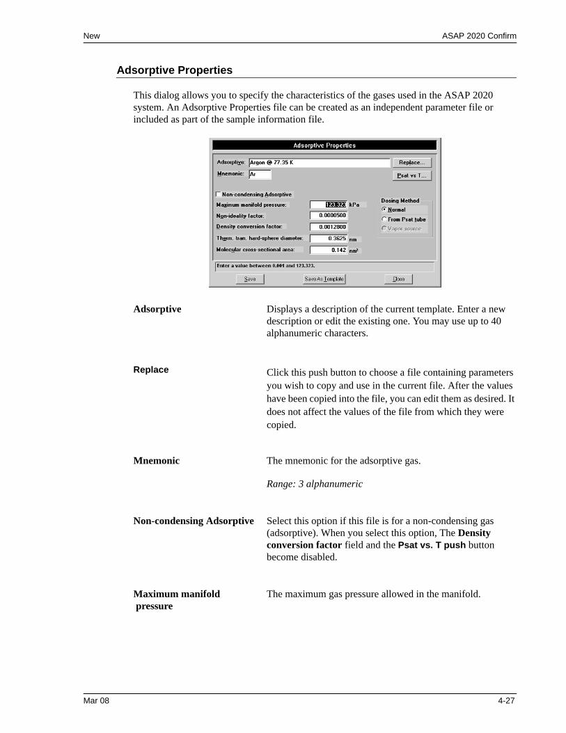
New ASAP 2020 Confirm
Adsorptive Properties
This dialog allows you to specify the characteristics of the gases used in the ASAP 2020 system. An Adsorptive Properties file can be created as an independent parameter file or included as part of the sample information file.
Adsorptive Displays a description of the current template. Enter a new description or edit the existing one. You may use up to 40 alphanumeric characters.
Replace Click this push button to choose a file containing parameters you wish to copy and use in the current file. After the values have been copied into the file, you can edit them as desired. It does not affect the values of the file from which they were copied.
Mnemonic The mnemonic for the adsorptive gas.
Range: 3 alphanumeric
Non-condensing Adsorptive Select this option if this file is for a non-condensing gas (adsorptive). When you select this option, The Density conversion factor field and the Psat vs. T push button become disabled.
Maximum manifold pressure
The maximum gas pressure allowed in the manifold.
Mar 08 4-27
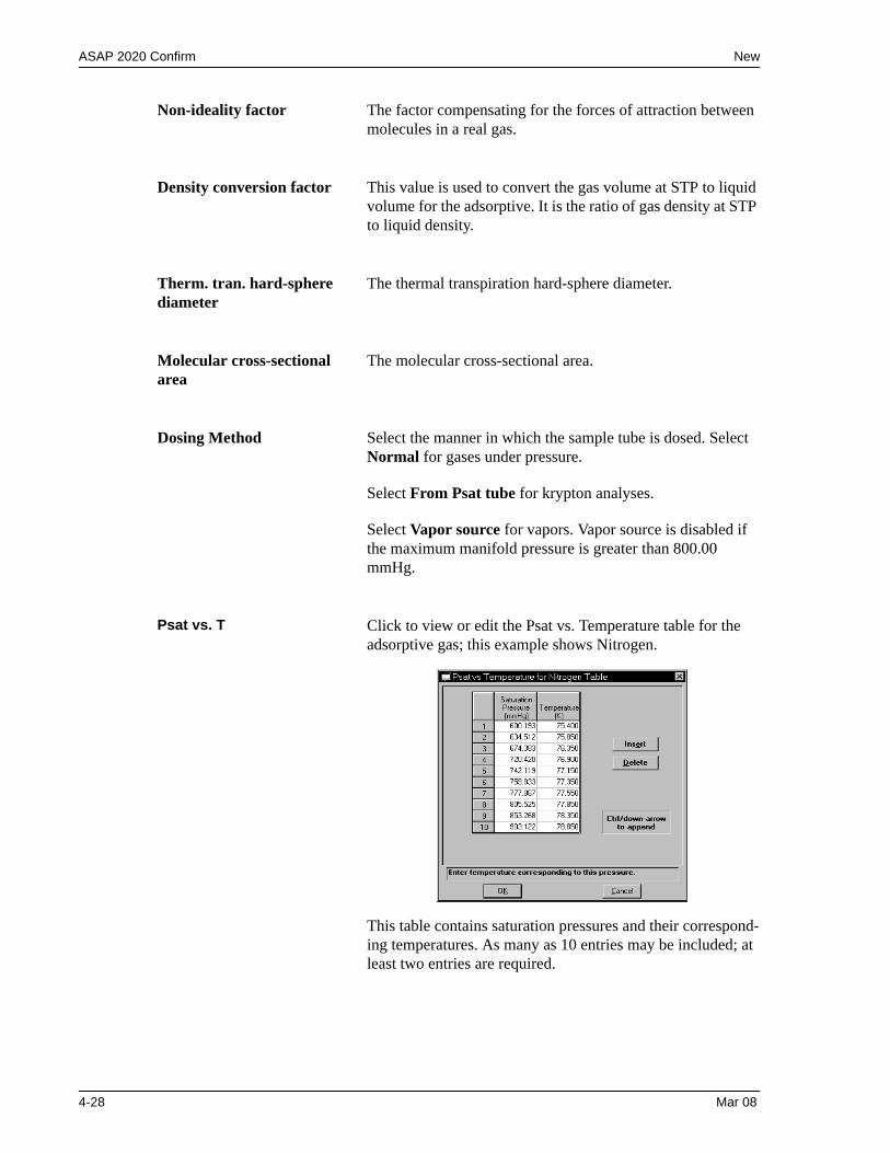
ASAP 2020 Confirm New
Non-ideality factor The factor compensating for the forces of attraction between molecules in a real gas.
Density conversion factor This value is used to convert the gas volume at STP to liquid volume for the adsorptive. It is the ratio of gas density at STP to liquid density.
Therm. tran. hard-sphere diameter
The thermal transpiration hard-sphere diameter.
Molecular cross-sectionalarea
The molecular cross-sectional area.
Dosing Method Select the manner in which the sample tube is dosed. Select Normal for gases under pressure.
Select From Psat tube for krypton analyses.
Select Vapor source for vapors. Vapor source is disabled if the maximum manifold pressure is greater than 800.00 mmHg.
Psat vs. T Click to view or edit the Psat vs. Temperature table for the adsorptive gas; this example shows Nitrogen.
This table contains saturation pressures and their correspond-ing temperatures. As many as 10 entries may be included; at least two entries are required.
4-28 Mar 08
New ASAP 2020 Confirm
Psat vs. T
(continued)
You can edit the table by clicking on the desired saturation pressure or temperature and entering a different value.
Use Insert to insert a new row above the selected line; the cursor moves to the new line. Use Delete to delete the selected row.
Save Displays the Save as Adsorptive Properties File dialog (see page 4-11 for an example of this dialog).
If the Save push button is not enabled, a file with the same ID currently exists. You must edit the identification of the current file before it can be saved. The ASAP 2020 Confirm program does not allow duplicate descriptions.
Save as Template Enables you to save all parameters of the current file as an adsorptive properties file template.
Close Closes the dialog box. If the file contains unsaved changes, you are prompted to save before the dialog box closes.
Mar 08 4-29
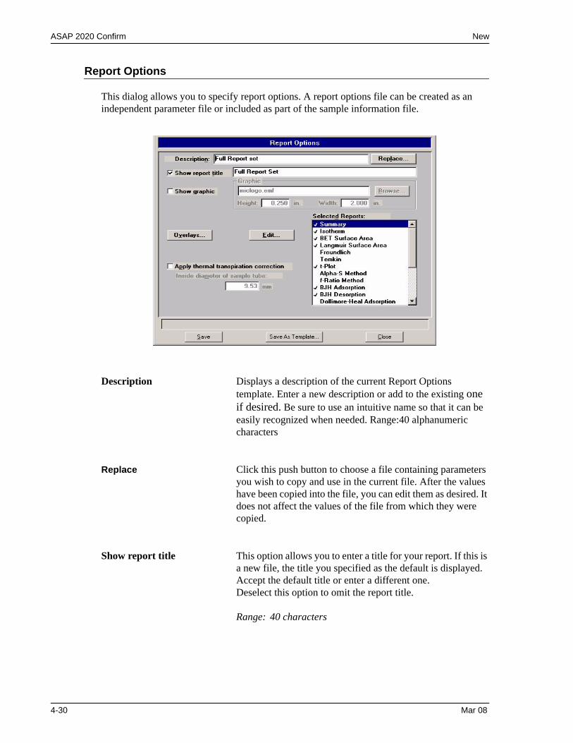
ASAP 2020 Confirm New
Report Options
This dialog allows you to specify report options. A report options file can be created as an independent parameter file or included as part of the sample information file.
Description Displays a description of the current Report Options template. Enter a new description or add to the existing one if desired. Be sure to use an intuitive name so that it can be easily recognized when needed. Range:40 alphanumeric characters
Replace Click this push button to choose a file containing parameters you wish to copy and use in the current file. After the values have been copied into the file, you can edit them as desired. It does not affect the values of the file from which they were copied.
Show report title This option allows you to enter a title for your report. If this is a new file, the title you specified as the default is displayed. Accept the default title or enter a different one.Deselect this option to omit the report title.
Range: 40 characters
4-30 Mar 08
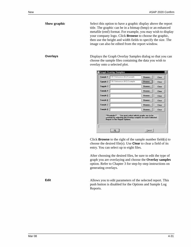
New ASAP 2020 Confirm
Show graphic Select this option to have a graphic display above the report title. The graphic can be in a bitmap (bmp) or an enhanced metafile (emf) format. For example, you may wish to display your company logo. Click Browse to choose the graphic, then use the height and width fields to specify the size. The image can also be edited from the report window.
Overlays Displays the Graph Overlay Samples dialog so that you can choose the sample files containing the data you wish to overlay onto a selected plot.
Click Browse to the right of the sample number field(s) to choose the desired file(s). Use Clear to clear a field of its entry. You can select up to eight files.
After choosing the desired files, be sure to edit the type of graph you are overlaying and choose the Overlay samples option. Refer to Chapter 3 for step-by-step instructions on generating overlays.
Edit Allows you to edit parameters of the selected report. This push button is disabled for the Options and Sample Log Reports.
Mar 08 4-31
ASAP 2020 Confirm New
Apply thermal transpiration correction
Select this option to correct for the temperature-induced pressure difference between the manifold and the chilled sample tube. This option is most significant for pressures less than approximately 1.0 mmHg. Never use filler rods in the sample tube when applying correction for thermal transpiration
You should always use thermal transpiration when performing micropore analyses.
Inside diameter of sample tube
Enabled when you select Thermal transpiration correction, so that you may enter the inside diameter of the sample tube.
Selected Reports Contains a list of available reports. Choose reports by double-clicking on the desired report(s). Alternatively, you can highlight the desired report and press the Spacebar. A report is selected when it is preceded with a check mark. You may deselect reports in the same manner.
• Summary• Isotherm• BET Surface Area• Langmuir Surface Area• Freundlich• Temkin • t-Plot• Alpha-S Method• f-Ratio Method• BJH Adsorption • BJH Desorption• Dollimore-Heal Adsorption• Dollimore-Heal Desorptioin• Horvath-Kawazoe (if micropore option is installed)• DFT Pore Size• DFT Surface Energy• Dubinin• MP-Method• Options• Sample Log• Validation
Editing options for these reports are found in subsequent sections.
You can find printed examples of some reports in Chapter 6 beginning on page 6-27.
4-32 Mar 08
New ASAP 2020 Confirm
Save Displays the Save as Adsorptive Properties File dialog (see page 4-11 for an example of this dialog).
If the Save push button is not enabled, a file with the same ID currently exists. You must edit the identification of the current file before it can be saved. The ASAP 2020 Confirm program does not allow duplicate descriptions.
Save as Template Enables you to save all parameters of the current file as an adsorptive properties file template.
Close Closes the dialog. If the file contains unsaved changes, you are prompted to save before the dialog box closes.
Mar 08 4-33
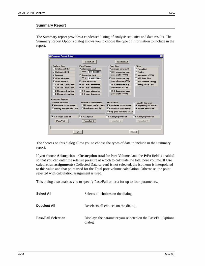
ASAP 2020 Confirm New
Summary Report
The Summary report provides a condensed listing of analysis statistics and data results. The Summary Report Options dialog allows you to choose the type of information to include in the report.
The choices on this dialog allow you to choose the types of data to include in the Summary report.
If you choose Adsorption or Desorption total for Pore Volume data, the P/Po field is enabled so that you can enter the relative pressure at which to calculate the total pore volume. If Use calculation assignments (Collected Data screen) is not selected, the isotherm is interpolated to this value and that point used for the Total pore volume calculation. Otherwise, the point selected with calculation assignment is used.
This dialog also enables you to specify Pass/Fail criteria for up to four parameters.
Select All Selects all choices on the dialog.
Deselect All Deselects all choices on the dialog.
Pass/Fail Selection Displays the parameter you selected on the Pass/Fail Options dialog.
4-34 Mar 08
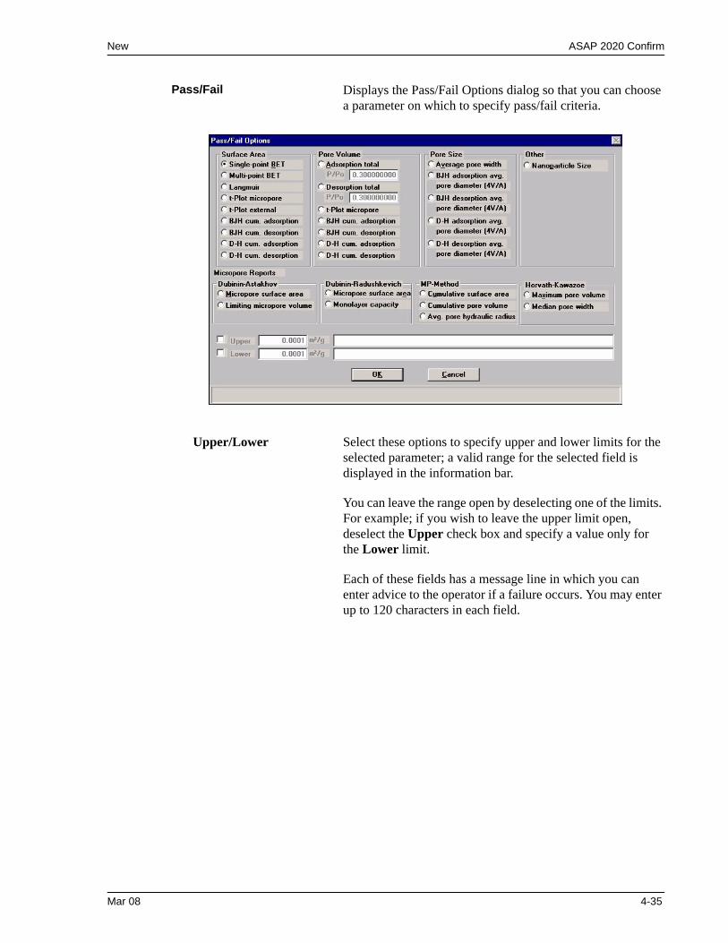
New ASAP 2020 Confirm
Pass/Fail Displays the Pass/Fail Options dialog so that you can choose a parameter on which to specify pass/fail criteria.
Upper/Lower Select these options to specify upper and lower limits for the selected parameter; a valid range for the selected field is displayed in the information bar.
You can leave the range open by deselecting one of the limits. For example; if you wish to leave the upper limit open, deselect the Upper check box and specify a value only for the Lower limit.
Each of these fields has a message line in which you can enter advice to the operator if a failure occurs. You may enter up to 120 characters in each field.
Mar 08 4-35
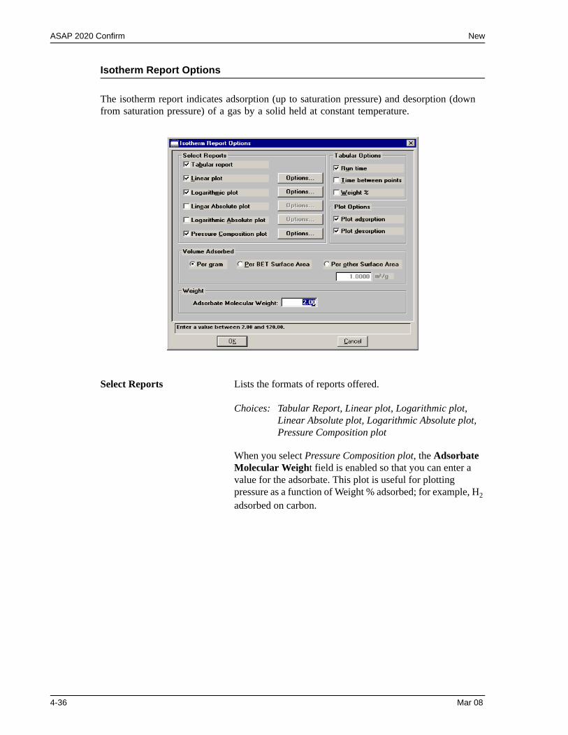
ASAP 2020 Confirm New
Isotherm Report Options
The isotherm report indicates adsorption (up to saturation pressure) and desorption (down from saturation pressure) of a gas by a solid held at constant temperature.
Select Reports Lists the formats of reports offered.
Choices: Tabular Report, Linear plot, Logarithmic plot, Linear Absolute plot, Logarithmic Absolute plot,
Pressure Composition plot
When you select Pressure Composition plot, the Adsorbate Molecular Weight field is enabled so that you can enter a value for the adsorbate. This plot is useful for plotting pressure as a function of Weight % adsorbed; for example, H2 adsorbed on carbon.
4-36 Mar 08
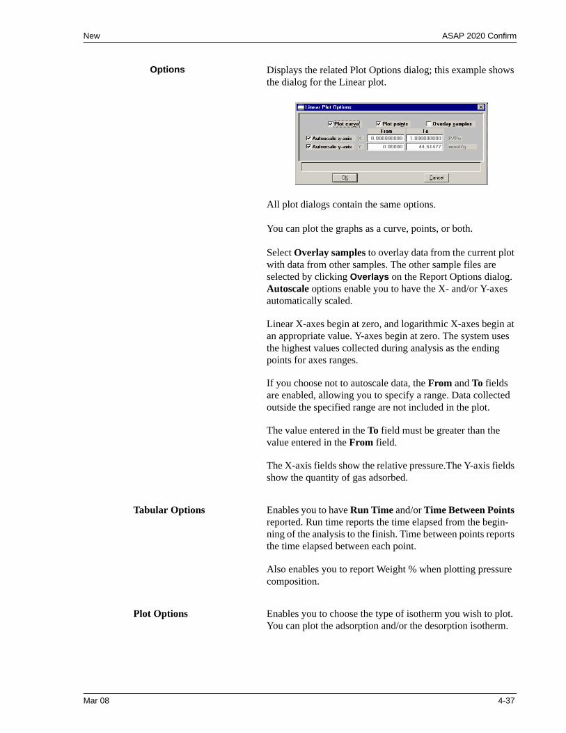
New ASAP 2020 Confirm
Options Displays the related Plot Options dialog; this example shows the dialog for the Linear plot.
All plot dialogs contain the same options.
You can plot the graphs as a curve, points, or both.
Select Overlay samples to overlay data from the current plot with data from other samples. The other sample files are selected by clicking Overlays on the Report Options dialog.Autoscale options enable you to have the X- and/or Y-axes automatically scaled.
Linear X-axes begin at zero, and logarithmic X-axes begin at an appropriate value. Y-axes begin at zero. The system uses the highest values collected during analysis as the ending points for axes ranges.
If you choose not to autoscale data, the From and To fields are enabled, allowing you to specify a range. Data collected outside the specified range are not included in the plot.
The value entered in the To field must be greater than the value entered in the From field.
The X-axis fields show the relative pressure.The Y-axis fields show the quantity of gas adsorbed.
Tabular Options Enables you to have Run Time and/or Time Between Points reported. Run time reports the time elapsed from the begin-ning of the analysis to the finish. Time between points reports the time elapsed between each point.
Also enables you to report Weight % when plotting pressure composition.
Plot Options Enables you to choose the type of isotherm you wish to plot. You can plot the adsorption and/or the desorption isotherm.
Mar 08 4-37

ASAP 2020 Confirm New
Volume Adsorbed Enables you to choose the manner in which the volume adsorbed is reported. These data are reported by default as Per Gram (cm3/g). However, you can choose to report data Per BET Surface Area (cm3/m2) or Per Other Surface Area (m2/g). If the latter field is selected, a field is enabled allowing you to enter a value.
Weight The Adsorbate Molecular Weight field is enabled when you choose Pressure Composition plot, allowing you to enter the molecular weight of the adsorbate.
4-38 Mar 08
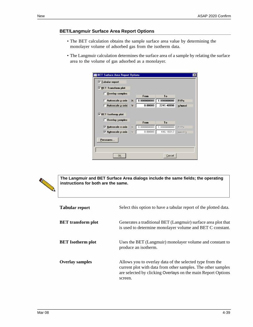
New ASAP 2020 Confirm
BET/Langmuir Surface Area Report Options
• The BET calculation obtains the sample surface area value by determining the monolayer volume of adsorbed gas from the isotherm data.
• The Langmuir calculation determines the surface area of a sample by relating the surface area to the volume of gas adsorbed as a monolayer.
The Langmuir and BET Surface Area dialogs include the same fields; the operating instructions for both are the same.
Tabular report Select this option to have a tabular report of the plotted data.
BET transform plot Generates a traditional BET (Langmuir) surface area plot that is used to determine monolayer volume and BET C constant.
BET Isotherm plot Uses the BET (Langmuir) monolayer volume and constant to produce an isotherm.
Overlay samples Allows you to overlay data of the selected type from the current plot with data from other samples. The other samples are selected by clicking Overlays on the main Report Options screen.
Mar 08 4-39
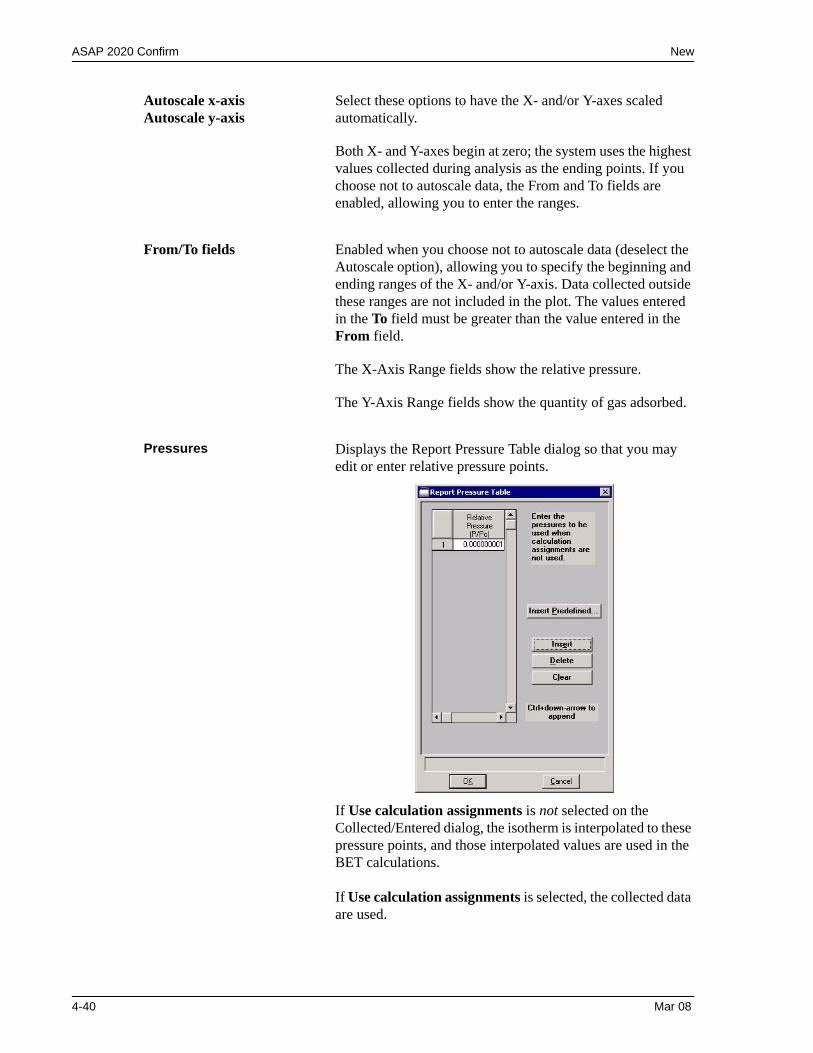
ASAP 2020 Confirm New
Autoscale x-axis Autoscale y-axis
Select these options to have the X- and/or Y-axes scaled automatically.
Both X- and Y-axes begin at zero; the system uses the highest values collected during analysis as the ending points. If you choose not to autoscale data, the From and To fields are enabled, allowing you to enter the ranges.
From/To fields Enabled when you choose not to autoscale data (deselect the Autoscale option), allowing you to specify the beginning and ending ranges of the X- and/or Y-axis. Data collected outside these ranges are not included in the plot. The values entered in the To field must be greater than the value entered in the From field.
The X-Axis Range fields show the relative pressure.
The Y-Axis Range fields show the quantity of gas adsorbed.
Pressures Displays the Report Pressure Table dialog so that you may edit or enter relative pressure points.
If Use calculation assignments is not selected on the Collected/Entered dialog, the isotherm is interpolated to these pressure points, and those interpolated values are used in the BET calculations.
If Use calculation assignments is selected, the collected data are used.
4-40 Mar 08
New ASAP 2020 Confirm
Insert predefined Displays the Surface Area Report Pressure Selection dialog, allowing you to select predefined points.
Choices: 1 Point, 3 Point, 5 Point, 5 Point Low Pressure
Insert Inserts a row into the table above the selected line.
Delete Deletes the selected row.
Clear Removes all but one entry from the table; one entry is required. The rows do not have to be selected.
A warning message requesting confirmation is displayed before the table is cleared.
Mar 08 4-41
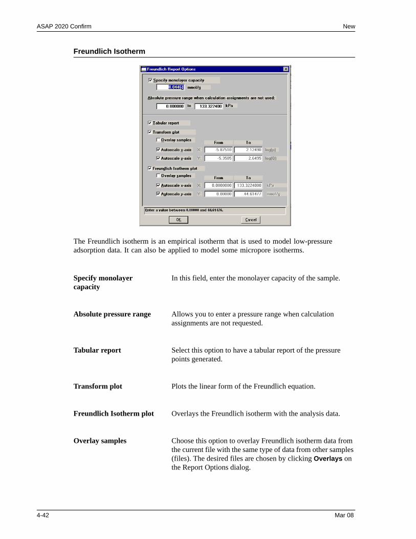
ASAP 2020 Confirm New
Freundlich Isotherm
The Freundlich isotherm is an empirical isotherm that is used to model low-pressure adsorption data. It can also be applied to model some micropore isotherms.
Specify monolayer capacity
In this field, enter the monolayer capacity of the sample.
Absolute pressure range Allows you to enter a pressure range when calculation assignments are not requested.
Tabular report Select this option to have a tabular report of the pressure points generated.
Transform plot Plots the linear form of the Freundlich equation.
Freundlich Isotherm plot Overlays the Freundlich isotherm with the analysis data.
Overlay samples Choose this option to overlay Freundlich isotherm data from the current file with the same type of data from other samples (files). The desired files are chosen by clicking Overlays on the Report Options dialog.
4-42 Mar 08
New ASAP 2020 Confirm
Autoscale x-axisAutoscale y-axis
Select these options to have the X- and/or Y-axis scaled automatically.
Both X- and Y-axes begin at zero; the system uses the highest values collected during analysis as the ending points.If you choose not to autoscale data, the From and To fields are enabled, allowing you to enter the ranges.
The X-axis shows the log of absolute pressure and the Y-axis shows the quantity of gas adsorbed.
From/To fields Enabled when you choose not to autoscale data (deselect the Autoscale option), allowing you to specify the beginning and ending ranges of the X- and/or Y-axis. Data collected outside these ranges are not included in the plot.
Mar 08 4-43
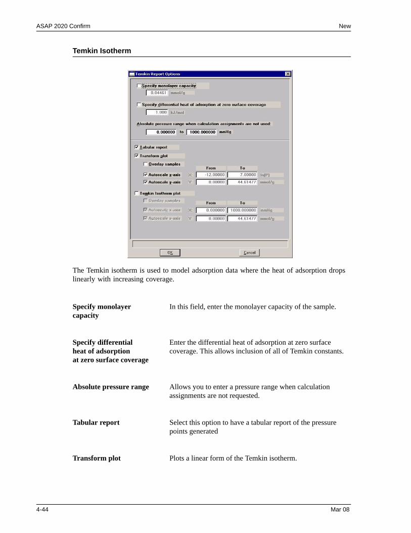
ASAP 2020 Confirm New
Temkin Isotherm
The Temkin isotherm is used to model adsorption data where the heat of adsorption drops linearly with increasing coverage.
Specify monolayer capacity
In this field, enter the monolayer capacity of the sample.
Specify differential heat of adsorption at zero surface coverage
Enter the differential heat of adsorption at zero surface coverage. This allows inclusion of all of Temkin constants.
Absolute pressure range Allows you to enter a pressure range when calculation assignments are not requested.
Tabular report Select this option to have a tabular report of the pressure points generated
Transform plot Plots a linear form of the Temkin isotherm.
4-44 Mar 08
New ASAP 2020 Confirm
Temkin isotherm plot Overlays the Temkin isotherm with the analysis data.
Overlay samples Choose this option to overlay Freundlich isotherm data from the current file with the same type of data from other samples (files). The desired files are chosen by selecting Overlays on the Report Options dialog.
Autoscale x-axisAutoscale y-axis
Select these options to have the X- and/or Y-axis scaled automatically.
Both X- and Y-axes begin at zero; the system uses the highest values collected during analysis as the ending points.
The X-axis shows the natural log of absolute pressure and the Y-axis shows the quantity of gas adsorbed.
If you choose not to autoscale data, the From and To fields are enabled, allowing you to enter the ranges.
From/To fields Enabled when you choose not to autoscale data (deselect the Autoscale option), allowing you to specify the beginning and ending ranges of the X- and/or Y-axis. Data collected outside these ranges are not included in the plot.
Mar 08 4-45
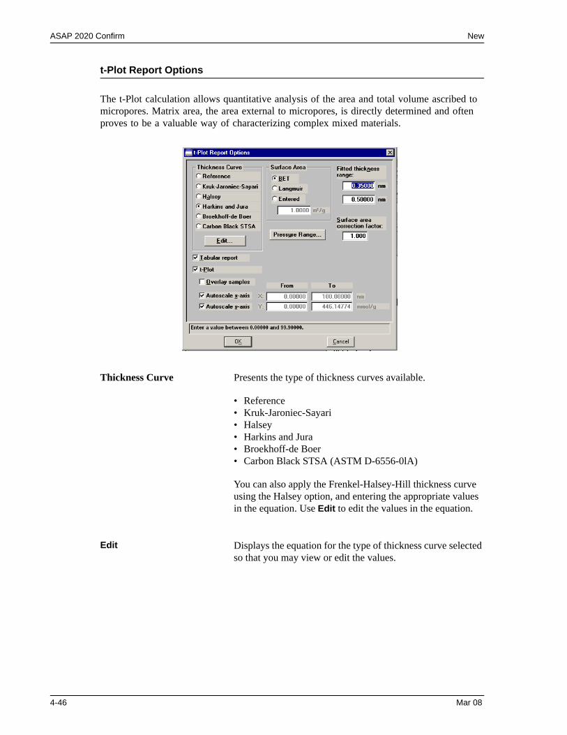
ASAP 2020 Confirm New
t-Plot Report Options
The t-Plot calculation allows quantitative analysis of the area and total volume ascribed to micropores. Matrix area, the area external to micropores, is directly determined and often proves to be a valuable way of characterizing complex mixed materials.
Thickness Curve Presents the type of thickness curves available.
• Reference• Kruk-Jaroniec-Sayari• Halsey• Harkins and Jura• Broekhoff-de Boer• Carbon Black STSA (ASTM D-6556-0lA)
You can also apply the Frenkel-Halsey-Hill thickness curve using the Halsey option, and entering the appropriate values in the equation. Use Edit to edit the values in the equation.
Edit Displays the equation for the type of thickness curve selected so that you may view or edit the values.
4-46 Mar 08
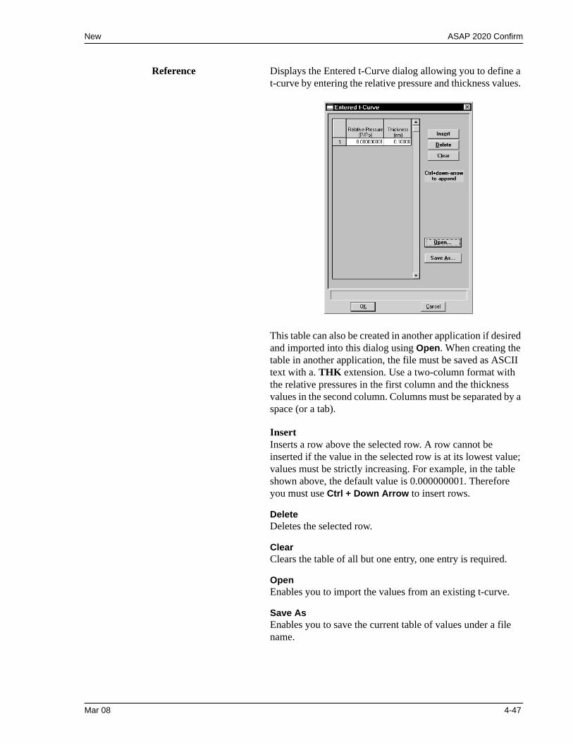
New ASAP 2020 Confirm
Reference Displays the Entered t-Curve dialog allowing you to define a t-curve by entering the relative pressure and thickness values.
This table can also be created in another application if desired and imported into this dialog using Open. When creating the table in another application, the file must be saved as ASCII text with a. THK extension. Use a two-column format with the relative pressures in the first column and the thickness values in the second column. Columns must be separated by a space (or a tab).
InsertInserts a row above the selected row. A row cannot be inserted if the value in the selected row is at its lowest value; values must be strictly increasing. For example, in the table shown above, the default value is 0.000000001. Therefore you must use Ctrl + Down Arrow to insert rows.
DeleteDeletes the selected row.
ClearClears the table of all but one entry, one entry is required.
OpenEnables you to import the values from an existing t-curve.
Save AsEnables you to save the current table of values under a file name.
Mar 08 4-47
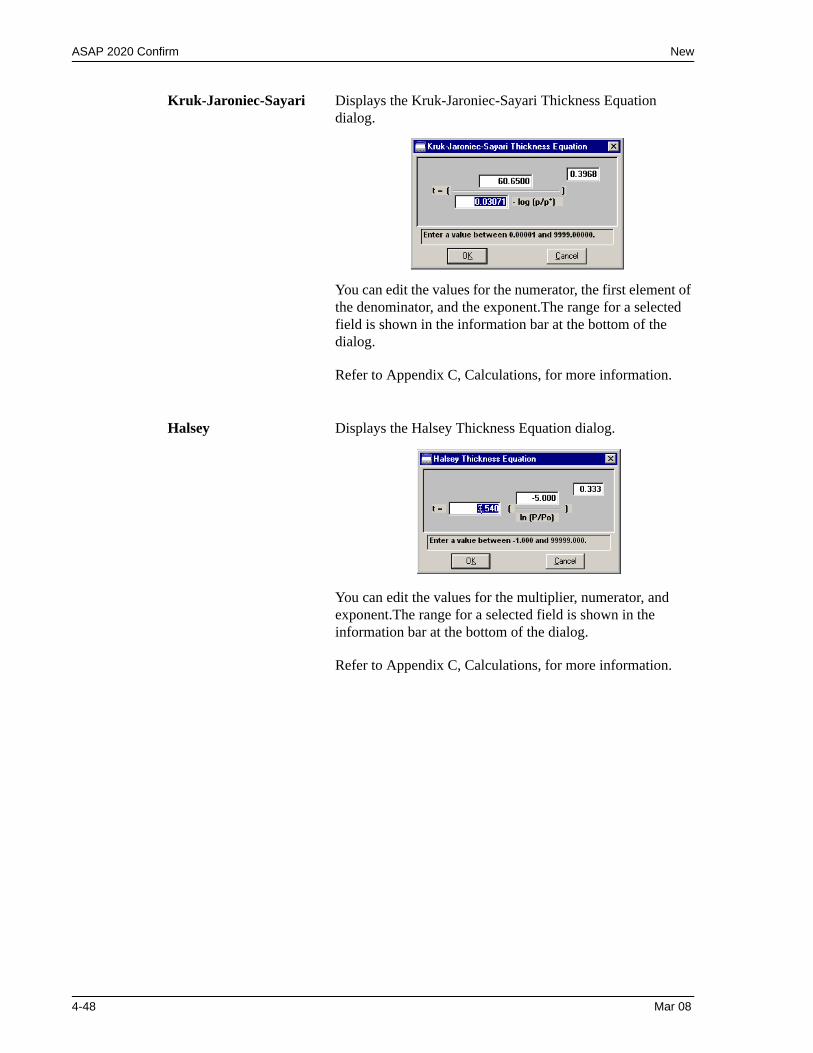
ASAP 2020 Confirm New
Kruk-Jaroniec-Sayari Displays the Kruk-Jaroniec-Sayari Thickness Equation dialog.
You can edit the values for the numerator, the first element of the denominator, and the exponent.The range for a selected field is shown in the information bar at the bottom of the dialog.
Refer to Appendix C, Calculations, for more information.
Halsey Displays the Halsey Thickness Equation dialog.
You can edit the values for the multiplier, numerator, and exponent.The range for a selected field is shown in the information bar at the bottom of the dialog.
Refer to Appendix C, Calculations, for more information.
4-48 Mar 08
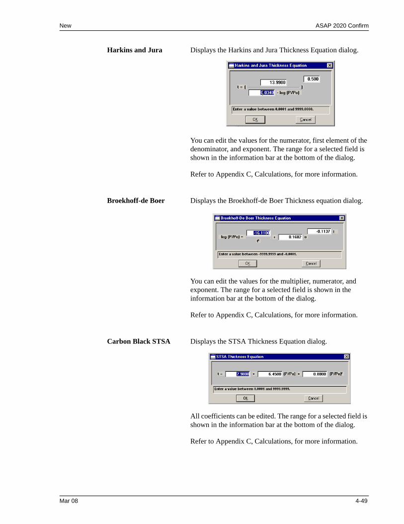
New ASAP 2020 Confirm
Harkins and Jura Displays the Harkins and Jura Thickness Equation dialog.
You can edit the values for the numerator, first element of the denominator, and exponent. The range for a selected field is shown in the information bar at the bottom of the dialog.
Refer to Appendix C, Calculations, for more information.
Broekhoff-de Boer Displays the Broekhoff-de Boer Thickness equation dialog.
You can edit the values for the multiplier, numerator, and exponent. The range for a selected field is shown in the information bar at the bottom of the dialog.
Refer to Appendix C, Calculations, for more information.
Carbon Black STSA Displays the STSA Thickness Equation dialog.
All coefficients can be edited. The range for a selected field is shown in the information bar at the bottom of the dialog.
Refer to Appendix C, Calculations, for more information.
Mar 08 4-49
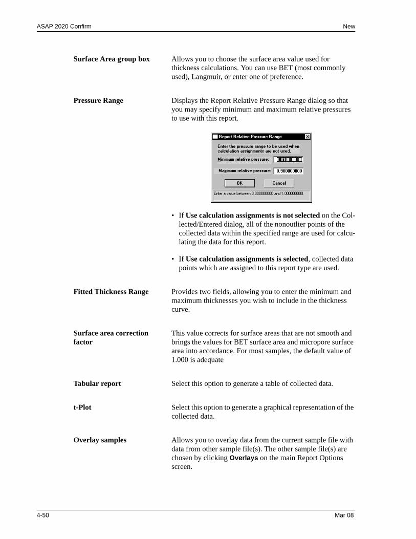
ASAP 2020 Confirm New
Surface Area group box Allows you to choose the surface area value used for thickness calculations. You can use BET (most commonly used), Langmuir, or enter one of preference.
Pressure Range Displays the Report Relative Pressure Range dialog so that you may specify minimum and maximum relative pressures to use with this report.
• If Use calculation assignments is not selected on the Col-lected/Entered dialog, all of the nonoutlier points of the collected data within the specified range are used for calcu-lating the data for this report.
• If Use calculation assignments is selected, collected data points which are assigned to this report type are used.
Fitted Thickness Range Provides two fields, allowing you to enter the minimum and maximum thicknesses you wish to include in the thickness curve.
Surface area correction factor
This value corrects for surface areas that are not smooth and brings the values for BET surface area and micropore surface area into accordance. For most samples, the default value of 1.000 is adequate
Tabular report Select this option to generate a table of collected data.
t-Plot Select this option to generate a graphical representation of the collected data.
Overlay samples Allows you to overlay data from the current sample file with data from other sample file(s). The other sample file(s) are chosen by clicking Overlays on the main Report Options screen.
4-50 Mar 08
New ASAP 2020 Confirm
Autoscale x-axis Autoscale y-axis
Select these options to have the X- and/or Y-axes scaled automatically.
Both X- and Y-axes begin at zero; the system uses the highest values collected during analysis as the ending points.
If you choose not to autoscale data, the From and To fields are enabled, allowing you to enter the ranges.
From/To fields Enabled when you choose not to autoscale data (deselect the Autoscale option), allowing you to specify the beginning and ending ranges of the X- and/or Y-axis. Data collected outside these ranges are not included in the plot.
The X-Axis Range fields show the relative pressure
The Y-Axis Range fields show the quantity of gas adsorbed
Mar 08 4-51
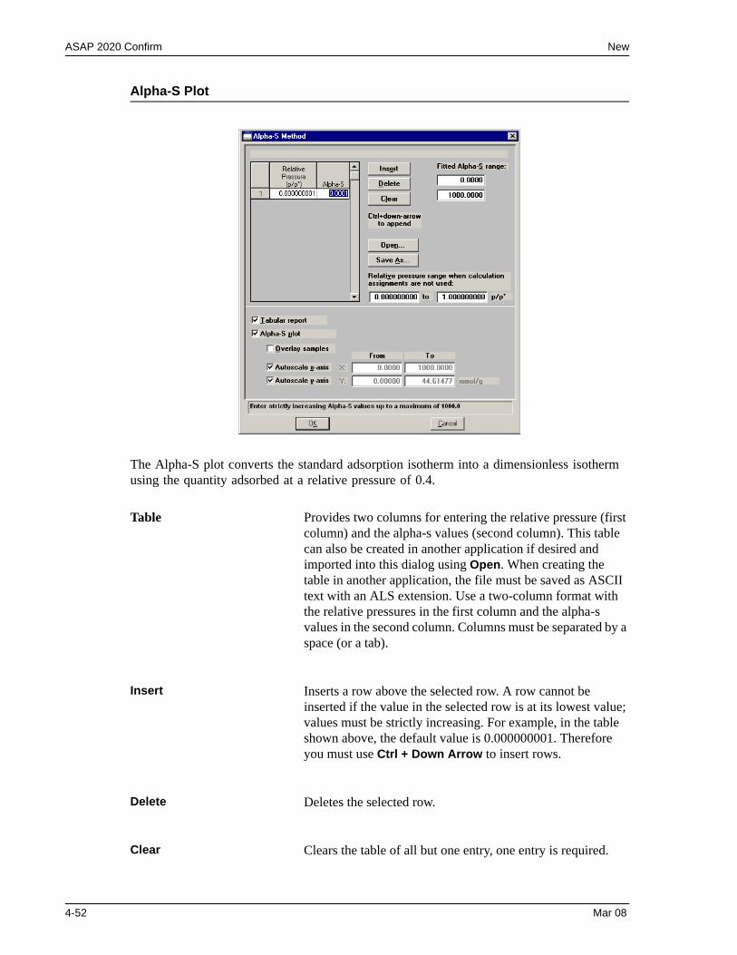
ASAP 2020 Confirm New
Alpha-S Plot
The Alpha-S plot converts the standard adsorption isotherm into a dimensionless isotherm using the quantity adsorbed at a relative pressure of 0.4.
Table Provides two columns for entering the relative pressure (first column) and the alpha-s values (second column). This table can also be created in another application if desired and imported into this dialog using Open. When creating the table in another application, the file must be saved as ASCII text with an ALS extension. Use a two-column format with the relative pressures in the first column and the alpha-s values in the second column. Columns must be separated by a space (or a tab).
Insert Inserts a row above the selected row. A row cannot be inserted if the value in the selected row is at its lowest value; values must be strictly increasing. For example, in the table shown above, the default value is 0.000000001. Therefore you must use Ctrl + Down Arrow to insert rows.
Delete Deletes the selected row.
Clear Clears the table of all but one entry, one entry is required.
4-52 Mar 08
New ASAP 2020 Confirm
Open Allows you to import the values from an existing alpha-s curve (ALS) into the table. One predefined curve is shipped with the analysis program. After the values are copied into the table, you may edit them if desired. Editing these values will not affect the file from which they were copied.
Save As Enables you to save the current table of values under a file name.
Fitted alpha-S Range Provides two fields for entering the minimum and maximum relative pressures from which the fit will be determined.
Relative pressure range Provides two fields for entering a pressure range when calculation assignments are not used.
Tabular report Select this option to generate collected data in a tabular manner.
Alpha-S plot Select this option to generate collected data graphically.
Overlay samples Allows you to overlay data from the current sample file with data from other sample file(s). The other sample file(s) are chosen by clicking Overlays on the main Report Options screen.
Autoscale x-axis Autoscale y-axis
Select these options to have the X- and/or Y-axes scaled automatically.
Both X- and Y-axes begin at zero; the system uses the highest values collected during analysis as the ending points.
If you choose not to autoscale data, the From and To fields are enabled, allowing you to enter the ranges.
Mar 08 4-53
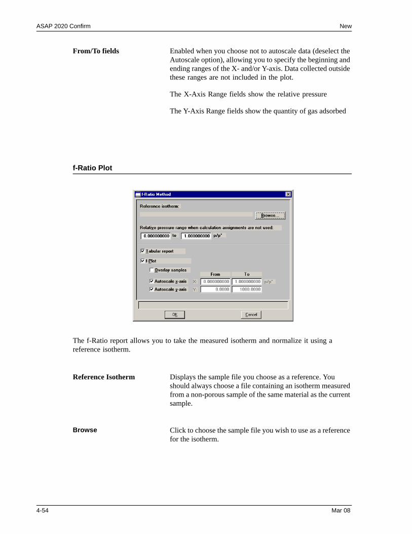
ASAP 2020 Confirm New
f-Ratio Plot
The f-Ratio report allows you to take the measured isotherm and normalize it using a reference isotherm.
From/To fields Enabled when you choose not to autoscale data (deselect the Autoscale option), allowing you to specify the beginning and ending ranges of the X- and/or Y-axis. Data collected outside these ranges are not included in the plot.
The X-Axis Range fields show the relative pressure
The Y-Axis Range fields show the quantity of gas adsorbed
Reference Isotherm Displays the sample file you choose as a reference. You should always choose a file containing an isotherm measured from a non-porous sample of the same material as the current sample.
Browse Click to choose the sample file you wish to use as a reference for the isotherm.
4-54 Mar 08
New ASAP 2020 Confirm
Relative pressure range Allows you to enter a pressure range when calculations assignments are not used.
Tabular report Choose this option to have a tabular report generated The tabular report contains four columns: relative pressure, quantity adsorbed for the isotherm of interest, quantity adsorbed for the reference isotherm, and the ratio of the quantities adsorbed.
f-Plot Choose this option to have the data plotted as a graph.
Overlay samples Allows you to overlay data from the current sample file with data from other sample file(s). The other sample file(s) are chosen by clicking Overlays on the main Report Options screen.
Autoscale x-axis Autoscale y-axis
Select these options to have the X- and/or Y-axes scaled automatically.
Both X- and Y-axes begin at zero; the system uses the highest values collected during analysis as the ending points.
If you choose not to autoscale data, the From and To fields are enabled, allowing you to enter the ranges.
From/To fields Enabled when you choose not to autoscale data (deselect the Autoscale option), allowing you to specify the beginning and ending ranges of the X- and/or Y-axis. Data collected outside these ranges are not included in the plot.
Mar 08 4-55
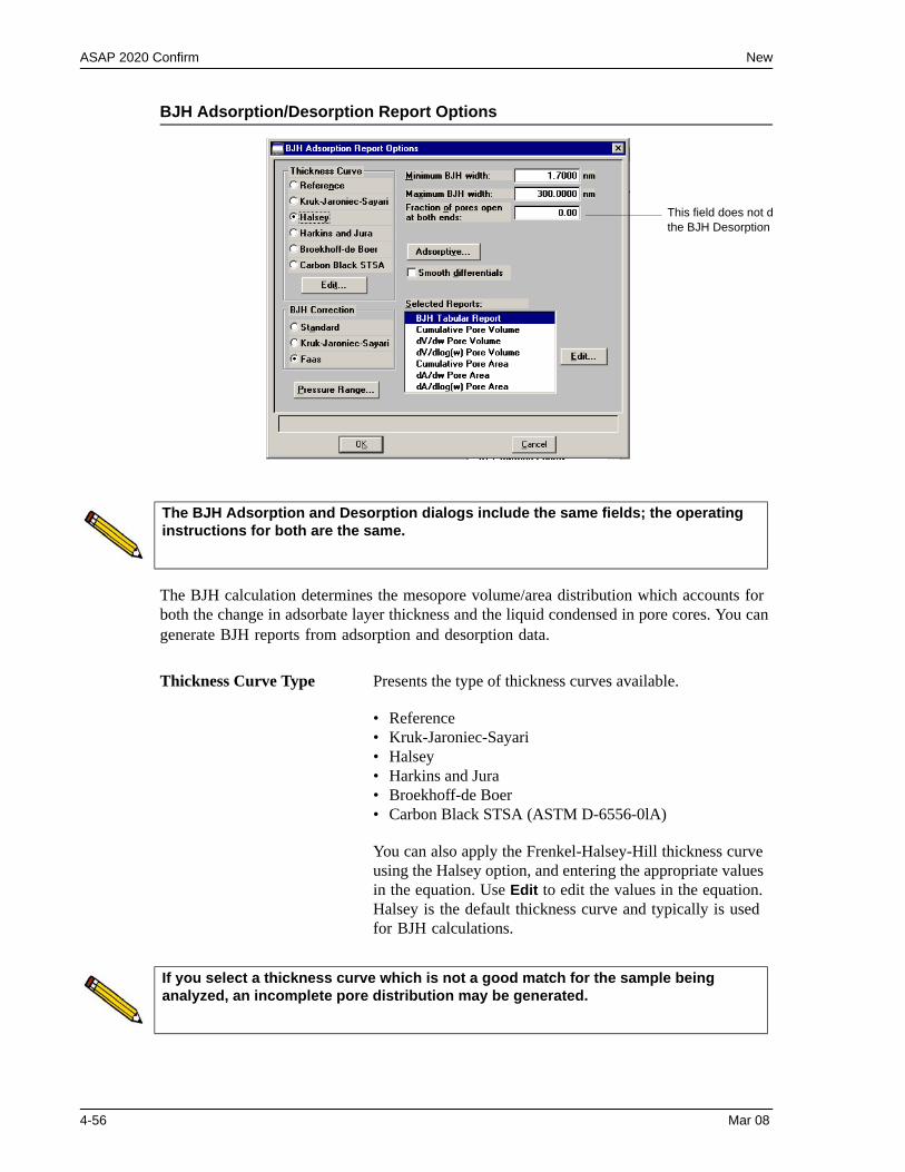
ASAP 2020 Confirm New
BJH Adsorption/Desorption Report Options
The BJH calculation determines the mesopore volume/area distribution which accounts for both the change in adsorbate layer thickness and the liquid condensed in pore cores. You can generate BJH reports from adsorption and desorption data.
This field does not dthe BJH Desorption
The BJH Adsorption and Desorption dialogs include the same fields; the operating instructions for both are the same.
Thickness Curve Type Presents the type of thickness curves available.
• Reference• Kruk-Jaroniec-Sayari• Halsey• Harkins and Jura• Broekhoff-de Boer• Carbon Black STSA (ASTM D-6556-0lA)
You can also apply the Frenkel-Halsey-Hill thickness curve using the Halsey option, and entering the appropriate values in the equation. Use Edit to edit the values in the equation. Halsey is the default thickness curve and typically is used for BJH calculations.
If you select a thickness curve which is not a good match for the sample being analyzed, an incomplete pore distribution may be generated.
4-56 Mar 08
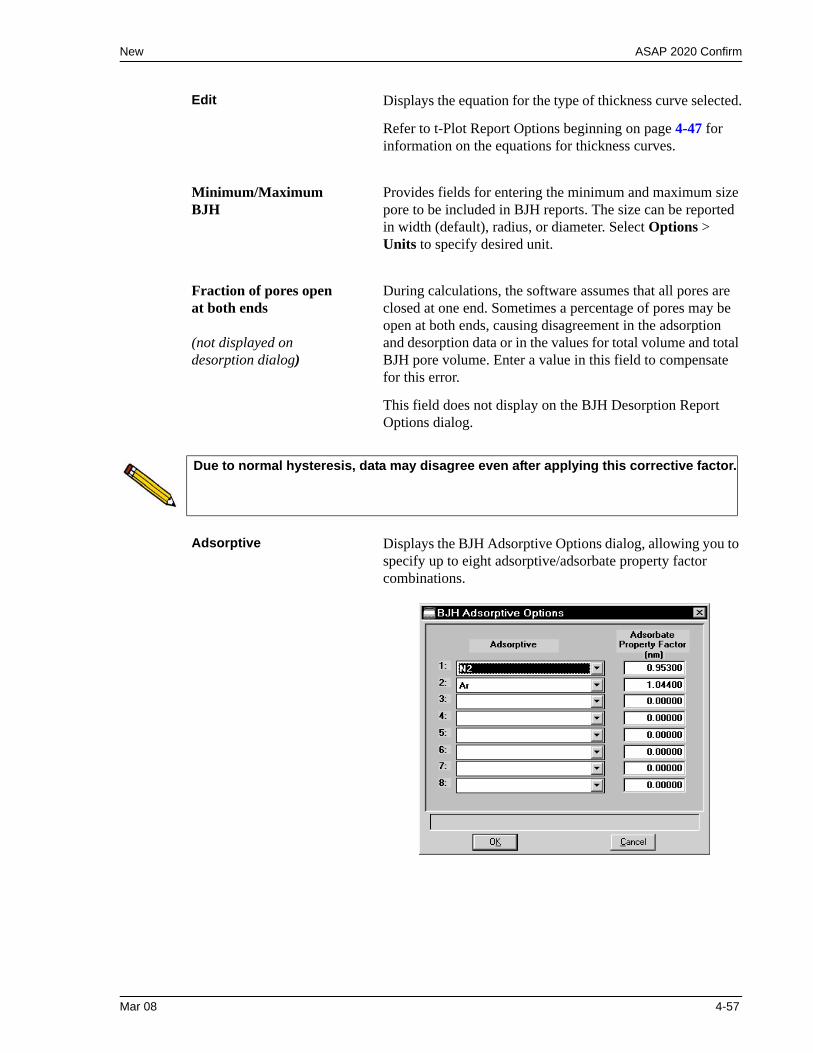
New ASAP 2020 Confirm
Edit Displays the equation for the type of thickness curve selected.
Refer to t-Plot Report Options beginning on page 4-47 for information on the equations for thickness curves.
Minimum/Maximum BJH
Provides fields for entering the minimum and maximum size pore to be included in BJH reports. The size can be reported in width (default), radius, or diameter. Select Options > Units to specify desired unit.
Fraction of pores open at both ends
(not displayed on desorption dialog)
During calculations, the software assumes that all pores are closed at one end. Sometimes a percentage of pores may be open at both ends, causing disagreement in the adsorption and desorption data or in the values for total volume and total BJH pore volume. Enter a value in this field to compensate for this error.
This field does not display on the BJH Desorption Report Options dialog.
Due to normal hysteresis, data may disagree even after applying this corrective factor.
Adsorptive Displays the BJH Adsorptive Options dialog, allowing you to specify up to eight adsorptive/adsorbate property factor combinations.
Mar 08 4-57
ASAP 2020 Confirm New
Adsorptive(continued)
The recommended adsorptives and their values are shown. You may specify up to six additional adsorptive/adsorbate property factor combinations.
The adsorbate property factor is the combination of constants in the numerator of the BJH equation which is specific to the type of gas used. Adsorbate property factors may be specified in angstroms or nanometers. Select Options > Units to spec-ify desired units.
Smooth differentials Smooths all of the differential calculations, eliminating varia-tions in the differential computation caused by noise in the input data.
BJH Correction Enables you to choose the type of correction to apply to calculations. The type you choose will be displayed in the report header.
Standard Uses original BJH models.
Kruk-Jaroniec-Sayari Good for reference thickness curves.
Faas Good for statistical thickness curves.
Pressure Range Displays the Report Relative Pressure Range dialog so that you may specify minimum and maximum relative pressures to use with this report.
• If Use calculation assignments is not selected on the Col-lected/Entered dialog, all of the nonoutlier points of the collected data within the specified range are used for calcu-lating the data for this report.
• If Use calculation assignments is selected, collected data points which are assigned to this report type are used.
4-58 Mar 08
New ASAP 2020 Confirm
Selected Reports Lists the available BJH reports.
• Tabular Report • Cumulative Pore Volume• dV/d* Pore Volume• dV/dlog(*) Pore Volume• Cumulative Pore Area• dA/d* Pore Area• dA/dlog(*) Pore Area
* = width, radius, or diameter
Choose a report by double-clicking on the report name or click the report name and press Spacebar. A report is selected when it is preceded with a check mark.
Edit Displays an associated dialog for the selected report. Editing options for available reports are shown in subsequent sections.
Mar 08 4-59
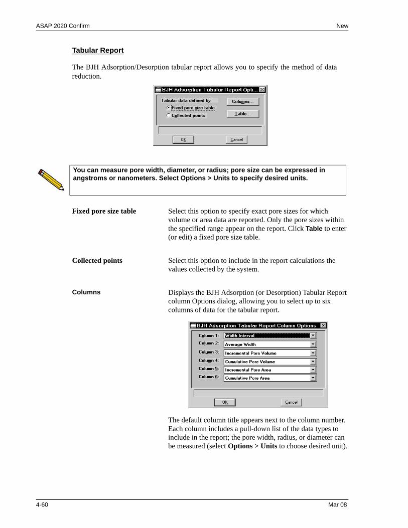
ASAP 2020 Confirm New
Tabular Report
The BJH Adsorption/Desorption tabular report allows you to specify the method of data reduction.
You can measure pore width, diameter, or radius; pore size can be expressed in angstroms or nanometers. Select Options > Units to specify desired units.
Fixed pore size table Select this option to specify exact pore sizes for which volume or area data are reported. Only the pore sizes within the specified range appear on the report. Click Table to enter (or edit) a fixed pore size table.
Collected points Select this option to include in the report calculations the values collected by the system.
Columns Displays the BJH Adsorption (or Desorption) Tabular Report column Options dialog, allowing you to select up to six columns of data for the tabular report.
The default column title appears next to the column number. Each column includes a pull-down list of the data types to include in the report; the pore width, radius, or diameter can be measured (select Options > Units to choose desired unit).
4-60 Mar 08
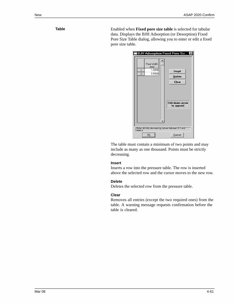
New ASAP 2020 Confirm
Table Enabled when Fixed pore size table is selected for tabular data. Displays the BJH Adsorption (or Desorption) Fixed Pore Size Table dialog, allowing you to enter or edit a fixed pore size table.
The table must contain a minimum of two points and may include as many as one thousand. Points must be strictly decreasing.
InsertInserts a row into the pressure table. The row is inserted above the selected row and the cursor moves to the new row.
DeleteDeletes the selected row from the pressure table.
ClearRemoves all entries (except the two required ones) from the table. A warning message requests confirmation before the table is cleared.
Mar 08 4-61
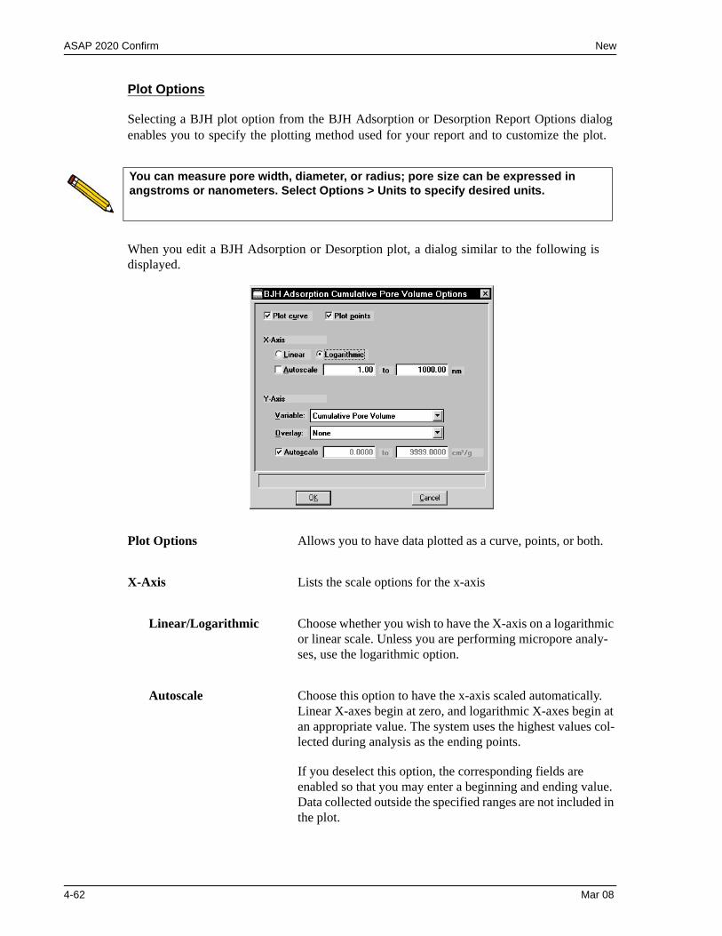
ASAP 2020 Confirm New
Plot Options
Selecting a BJH plot option from the BJH Adsorption or Desorption Report Options dialog enables you to specify the plotting method used for your report and to customize the plot.
When you edit a BJH Adsorption or Desorption plot, a dialog similar to the following is displayed.
You can measure pore width, diameter, or radius; pore size can be expressed in angstroms or nanometers. Select Options > Units to specify desired units.
Plot Options Allows you to have data plotted as a curve, points, or both.
X-Axis Lists the scale options for the x-axis
Linear/Logarithmic Choose whether you wish to have the X-axis on a logarithmic or linear scale. Unless you are performing micropore analy-ses, use the logarithmic option.
Autoscale Choose this option to have the x-axis scaled automatically. Linear X-axes begin at zero, and logarithmic X-axes begin at an appropriate value. The system uses the highest values col-lected during analysis as the ending points.
If you deselect this option, the corresponding fields are enabled so that you may enter a beginning and ending value. Data collected outside the specified ranges are not included in the plot.
4-62 Mar 08
New ASAP 2020 Confirm
Autoscale(continued)
X-axis range fields show pore radius or diameter in angstroms or nanometers.
Data ranges are displayed in the information bar across the bottom of the dialog when the cursor is in a numerical data entry field.
Y-axis Lists the options for the Y-axis.
Variable Click on the down-arrow to choose a variable for the Y-axis.
Overlay Displays a list of overlay choices. You can choose a different type of plot to overlay with the current plot. Or, you can choose Samples to overlay the current type of plot with the same type from other sample files. If you choose Samples, you select the other files using Overlays on the Report Options dialog.
Autoscale Choose this option to have the y-axis scaled automatically. Y-axes begin at zero. The system uses the highest values col-lected during analysis as the ending points.
If you deselect this option, the corresponding fields are enabled so that you may enter a beginning and ending value. Data collected outside the specified ranges are not included in the plot.
Y-axis range fields show the quantity of gas adsorbed.
Data ranges are displayed in the information bar across the bottom of the dialog when the cursor is in a numerical data entry field.
Mar 08 4-63
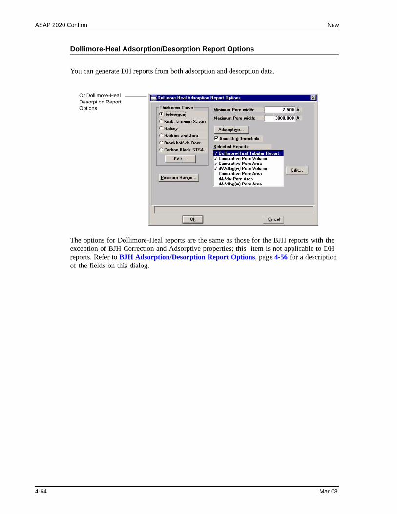
ASAP 2020 Confirm New
Dollimore-Heal Adsorption/Desorption Report Options
You can generate DH reports from both adsorption and desorption data.
The options for Dollimore-Heal reports are the same as those for the BJH reports with the exception of BJH Correction and Adsorptive properties; this item is not applicable to DH reports. Refer to BJH Adsorption/Desorption Report Options, page 4-56 for a description of the fields on this dialog.
Or Dollimore-Heal Desorption Report Options
4-64 Mar 08
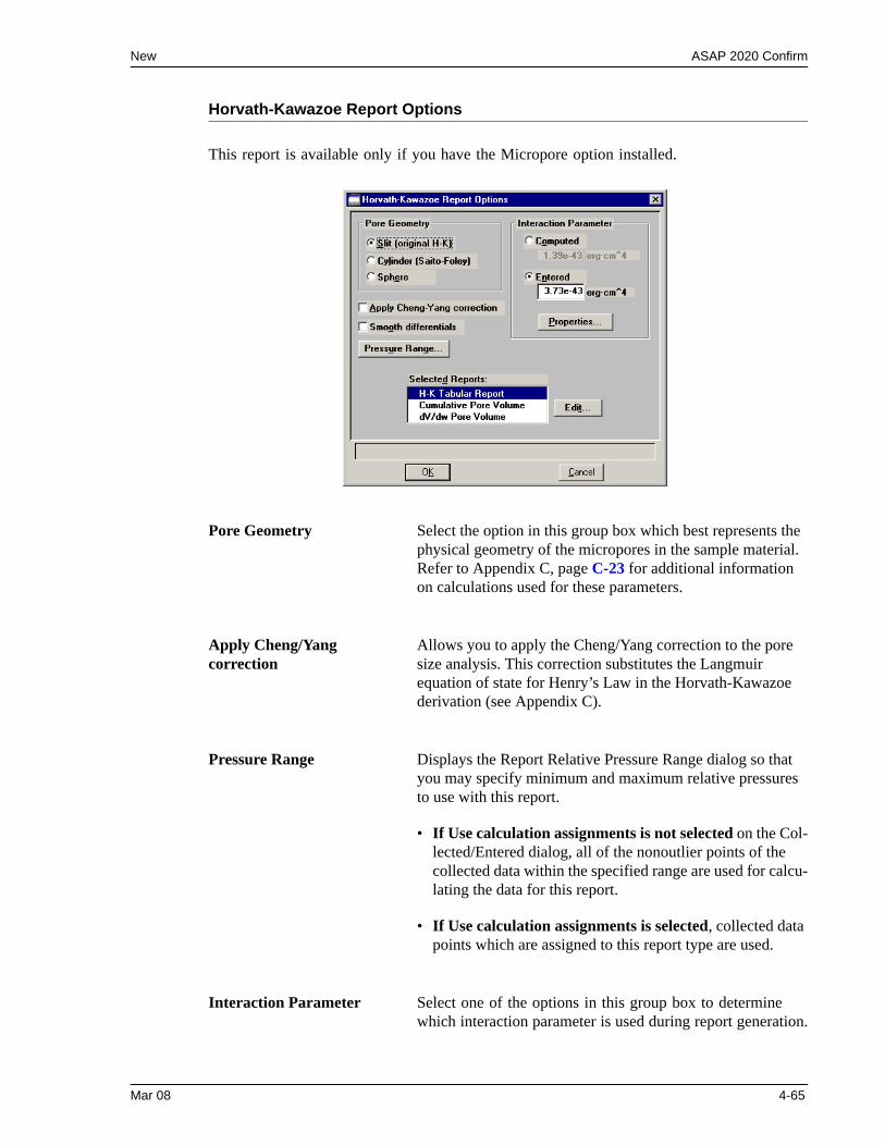
New ASAP 2020 Confirm
Horvath-Kawazoe Report Options
This report is available only if you have the Micropore option installed.
Pore Geometry Select the option in this group box which best represents the physical geometry of the micropores in the sample material. Refer to Appendix C, page C-23 for additional information on calculations used for these parameters.
Apply Cheng/Yang correction
Allows you to apply the Cheng/Yang correction to the pore size analysis. This correction substitutes the Langmuir equation of state for Henry’s Law in the Horvath-Kawazoe derivation (see Appendix C).
Pressure Range Displays the Report Relative Pressure Range dialog so that you may specify minimum and maximum relative pressures to use with this report.
• If Use calculation assignments is not selected on the Col-lected/Entered dialog, all of the nonoutlier points of the collected data within the specified range are used for calcu-lating the data for this report.
• If Use calculation assignments is selected, collected data points which are assigned to this report type are used.
Interaction Parameter Select one of the options in this group box to determine which interaction parameter is used during report generation.
Mar 08 4-65
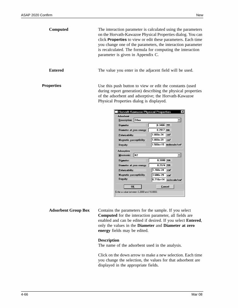
ASAP 2020 Confirm New
Computed The interaction parameter is calculated using the parameters on the Horvath-Kawazoe Physical Properties dialog. You can click Properties to view or edit these parameters. Each time you change one of the parameters, the interaction parameter is recalculated. The formula for computing the interaction parameter is given in Appendix C.
Entered The value you enter in the adjacent field will be used.
Properties Use this push button to view or edit the constants (used during report generation) describing the physical properties of the adsorbent and adsorptive; the Horvath-Kawazoe Physical Properties dialog is displayed.
Adsorbent Group Box Contains the parameters for the sample. If you select Computed for the interaction parameter, all fields are enabled and can be edited if desired. If you select Entered, only the values in the Diameter and Diameter at zero energy fields may be edited.
DescriptionThe name of the adsorbent used in the analysis.
Click on the down arrow to make a new selection. Each time you change the selection, the values for that adsorbent are displayed in the appropriate fields.
4-66 Mar 08
New ASAP 2020 Confirm
Adsorbent Group Box(continued)
DiameterThe diameter of the sample atom.
Diameter at zero energyThe diameter of an atom at zero interaction energy,(2/5)1/6 x diameter.
PolarizabilityThe polarizability of the adsorbent.
Magnetic susceptibilityThe magnetic susceptibility of the adsorbent.
DensityThe density per unit area of the adsorbent.
Adsorptive Group Box Contains the parameters for the adsorptives (provided with the software and/or user-defined). If you select Computed for the interaction parameter, all fields are enabled and can be edited if desired. If you select Entered, only the values in the Diameter and Diameter at zero energy fields may be edited.
MnemonicThe mnemonic name of the adsorptive gas in use.
Click on the down arrow to make a new selection. Each time you change the selection, the values for that adsorptive display in the appropriate fields. If no parameters have been defined, the default values are displayed.
DiameterThe diameter of the adsorptive atom.
Diameter at zero energyThe diameter of an atom at zero interaction energy,(2/5)1/6 x diameter.
PolarizabilityThe polarizability of the adsorptive.
Magnetic susceptibilityThe magnetic susceptibility of the adsorptive.
DensityThe density per unit area of the adsorptive.
Mar 08 4-67
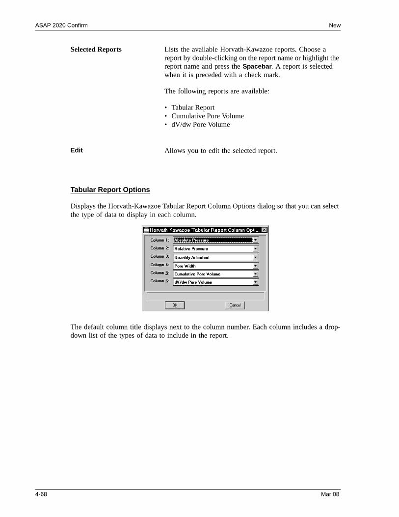
ASAP 2020 Confirm New
Tabular Report Options
Displays the Horvath-Kawazoe Tabular Report Column Options dialog so that you can select the type of data to display in each column.
The default column title displays next to the column number. Each column includes a drop-down list of the types of data to include in the report.
Selected Reports Lists the available Horvath-Kawazoe reports. Choose a report by double-clicking on the report name or highlight the report name and press the Spacebar. A report is selected when it is preceded with a check mark.
The following reports are available:
• Tabular Report• Cumulative Pore Volume• dV/dw Pore Volume
Edit Allows you to edit the selected report.
4-68 Mar 08
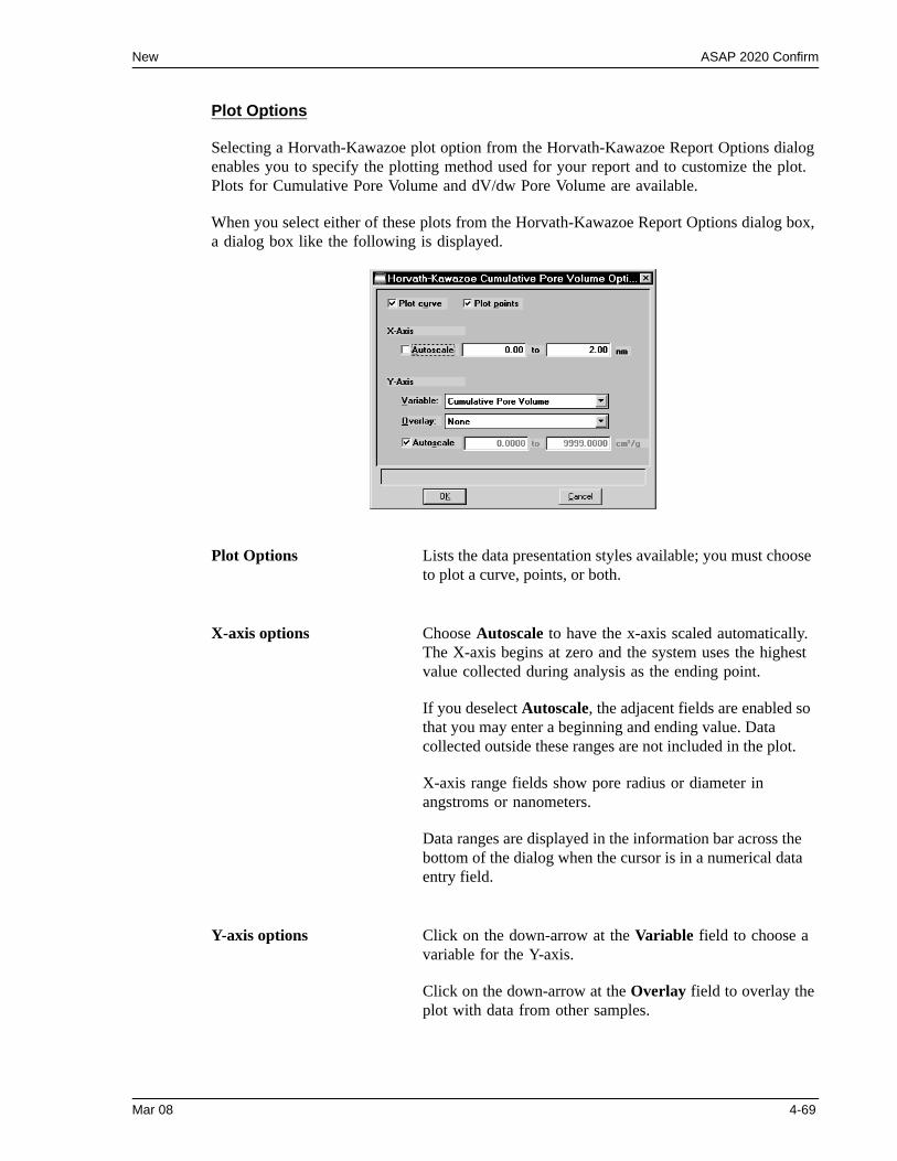
New ASAP 2020 Confirm
Plot Options
Selecting a Horvath-Kawazoe plot option from the Horvath-Kawazoe Report Options dialog enables you to specify the plotting method used for your report and to customize the plot. Plots for Cumulative Pore Volume and dV/dw Pore Volume are available.
When you select either of these plots from the Horvath-Kawazoe Report Options dialog box, a dialog box like the following is displayed.
Plot Options Lists the data presentation styles available; you must choose to plot a curve, points, or both.
X-axis options Choose Autoscale to have the x-axis scaled automatically. The X-axis begins at zero and the system uses the highest value collected during analysis as the ending point.
If you deselect Autoscale, the adjacent fields are enabled so that you may enter a beginning and ending value. Data collected outside these ranges are not included in the plot.
X-axis range fields show pore radius or diameter in angstroms or nanometers.
Data ranges are displayed in the information bar across the bottom of the dialog when the cursor is in a numerical data entry field.
Y-axis options Click on the down-arrow at the Variable field to choose a variable for the Y-axis.
Click on the down-arrow at the Overlay field to overlay the plot with data from other samples.
Mar 08 4-69

ASAP 2020 Confirm New
Y-axis options(continued)
Choose Autoscale to have the y-axis scaled automatically. Y-axes begin at zero. The system uses the highest value collected during analysis as the ending point.
If you deselect Autoscale, the corresponding fields are enabled so that you may enter a beginning and ending value. Data collected outside these ranges are not included in the plot.
Y-axis range fields show the quantity of gas adsorbed
Data ranges are displayed in the information bar across the bottom of the dialog when the cursor is in a numerical data entry field.
4-70 Mar 08
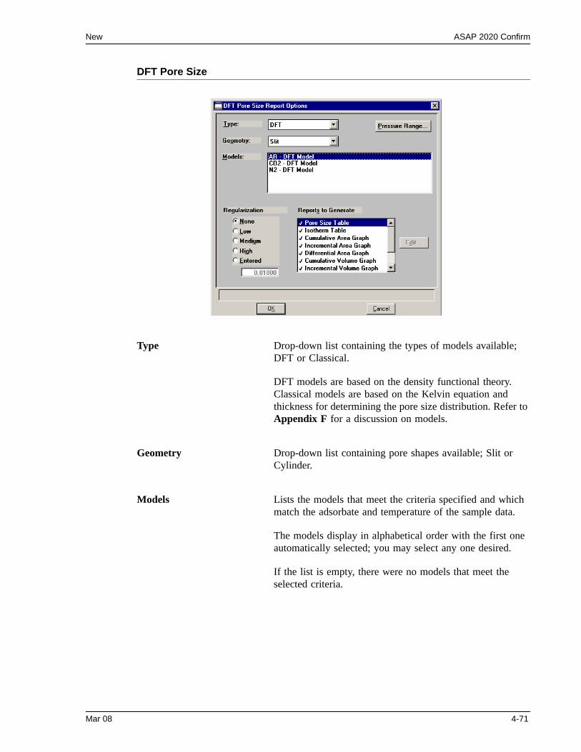
New ASAP 2020 Confirm
DFT Pore Size
Type Drop-down list containing the types of models available; DFT or Classical.
DFT models are based on the density functional theory. Classical models are based on the Kelvin equation and thickness for determining the pore size distribution. Refer to Appendix F for a discussion on models.
Geometry Drop-down list containing pore shapes available; Slit or Cylinder.
Models Lists the models that meet the criteria specified and which match the adsorbate and temperature of the sample data.
The models display in alphabetical order with the first one automatically selected; you may select any one desired.
If the list is empty, there were no models that meet the selected criteria.
Mar 08 4-71
ASAP 2020 Confirm New
Pressure Range Displays the Report Relative Pressure Range dialog so that you may specify minimum and maximum relative pressures to use with this report.
• If Use calculation assignments is not selected on the Col-lected/Entered dialog, all of the nonoutlier points of the collected data within the specified range are used for calcu-lating the data for this report.
• If Use calculation assignments is selected, collected data points which are assigned to this report type are used.
Regularization These choices enable you to choose the extent of smoothing you wish to have applied to your data, or your can choose None.
If you choose Entered, its field is enabled allowing you to enter a number giving a relative weight for the smoothing during deconvolution. Larger values produce more smoothing.
Reports to Generate Displays the types of reports available.
• Pore Size table• Isotherm table• Cumulative area graph• Incremental area graph• Differential area graph• Log goodness of fit graph• Goodness of fit graph
Graph details can be edited by selecting the Edit push button.
4-72 Mar 08
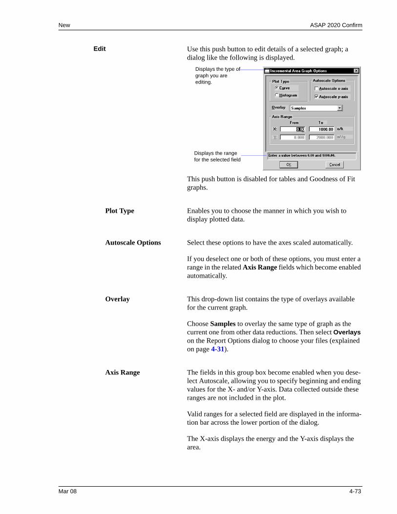
New ASAP 2020 Confirm
Edit Use this push button to edit details of a selected graph; a dialog like the following is displayed.
This push button is disabled for tables and Goodness of Fit graphs.
Plot Type Enables you to choose the manner in which you wish to display plotted data.
Autoscale Options Select these options to have the axes scaled automatically.
If you deselect one or both of these options, you must enter a range in the related Axis Range fields which become enabled automatically.
Overlay This drop-down list contains the type of overlays available for the current graph.
Choose Samples to overlay the same type of graph as the current one from other data reductions. Then select Overlays on the Report Options dialog to choose your files (explained on page 4-31).
Axis Range The fields in this group box become enabled when you dese-lect Autoscale, allowing you to specify beginning and ending values for the X- and/or Y-axis. Data collected outside these ranges are not included in the plot.
Valid ranges for a selected field are displayed in the informa-tion bar across the lower portion of the dialog.
The X-axis displays the energy and the Y-axis displays the area.
Displays the type of graph you are editing.
Displays the range for the selected field
Mar 08 4-73
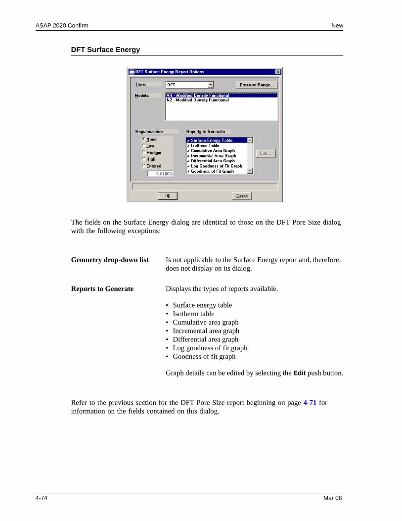
ASAP 2020 Confirm New
DFT Surface Energy
The fields on the Surface Energy dialog are identical to those on the DFT Pore Size dialog with the following exceptions:
Refer to the previous section for the DFT Pore Size report beginning on page 4-71 for information on the fields contained on this dialog.
Geometry drop-down list Is not applicable to the Surface Energy report and, therefore, does not display on its dialog.
Reports to Generate Displays the types of reports available.
• Surface energy table• Isotherm table• Cumulative area graph• Incremental area graph• Differential area graph• Log goodness of fit graph• Goodness of fit graph
Graph details can be edited by selecting the Edit push button.
4-74 Mar 08
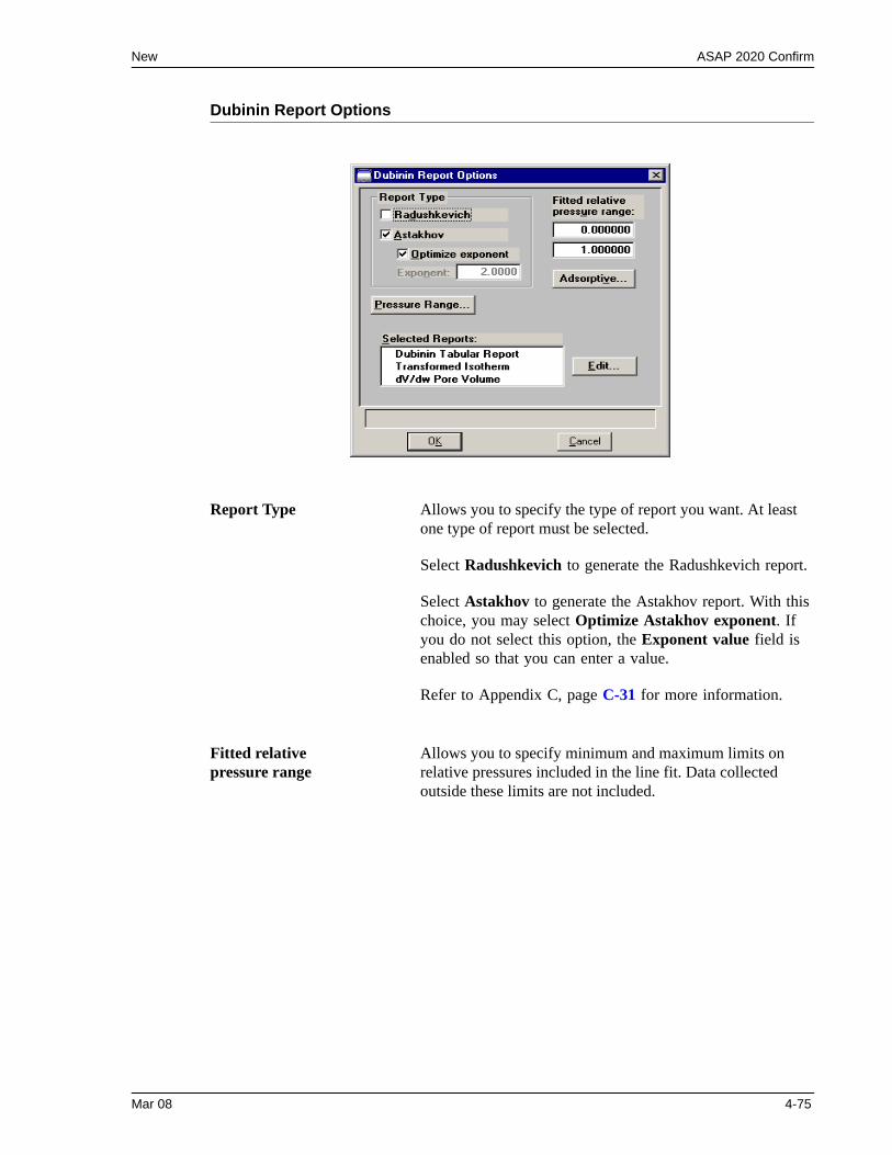
New ASAP 2020 Confirm
Dubinin Report Options
Report Type Allows you to specify the type of report you want. At least one type of report must be selected.
Select Radushkevich to generate the Radushkevich report.
Select Astakhov to generate the Astakhov report. With this choice, you may select Optimize Astakhov exponent. If you do not select this option, the Exponent value field is enabled so that you can enter a value.
Refer to Appendix C, page C-31 for more information.
Fitted relative pressure range
Allows you to specify minimum and maximum limits on relative pressures included in the line fit. Data collected outside these limits are not included.
Mar 08 4-75
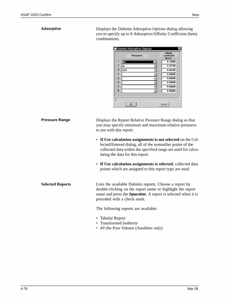
ASAP 2020 Confirm New
Adsorptive Displays the Dubinin Adsorptive Options dialog allowing you to specify up to 8 Adsorptive/Affinity Coefficient (beta) combinations.
Pressure Range Displays the Report Relative Pressure Range dialog so that you may specify minimum and maximum relative pressures to use with this report.
• If Use calculation assignments is not selected on the Col-lected/Entered dialog, all of the nonoutlier points of the collected data within the specified range are used for calcu-lating the data for this report.
• If Use calculation assignments is selected, collected data points which are assigned to this report type are used.
Selected Reports Lists the available Dubinin reports. Choose a report by double-clicking on the report name or highlight the report name and press the Spacebar. A report is selected when it is preceded with a check mark.
The following reports are available:
• Tabular Report• Transformed Isotherm• dV/dw Pore Volume (Astakhov only)
4-76 Mar 08
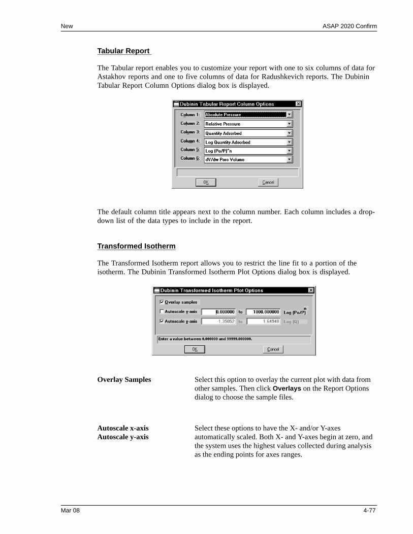
New ASAP 2020 Confirm
Tabular Report
The Tabular report enables you to customize your report with one to six columns of data for Astakhov reports and one to five columns of data for Radushkevich reports. The Dubinin Tabular Report Column Options dialog box is displayed.
The default column title appears next to the column number. Each column includes a drop-down list of the data types to include in the report.
Transformed Isotherm
The Transformed Isotherm report allows you to restrict the line fit to a portion of the isotherm. The Dubinin Transformed Isotherm Plot Options dialog box is displayed.
Overlay Samples Select this option to overlay the current plot with data from other samples. Then click Overlays on the Report Options dialog to choose the sample files.
Autoscale x-axisAutoscale y-axis
Select these options to have the X- and/or Y-axes automatically scaled. Both X- and Y-axes begin at zero, and the system uses the highest values collected during analysis as the ending points for axes ranges.
Mar 08 4-77
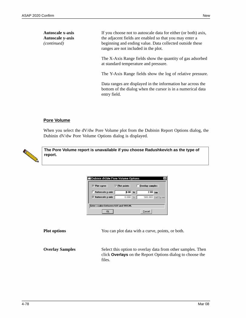
ASAP 2020 Confirm New
Pore Volume
When you select the dV/dw Pore Volume plot from the Dubinin Report Options dialog, the Dubinin dV/dw Pore Volume Options dialog is displayed.
Autoscale x-axisAutoscale y-axis(continued)
If you choose not to autoscale data for either (or both) axis, the adjacent fields are enabled so that you may enter a beginning and ending value. Data collected outside these ranges are not included in the plot.
The X-Axis Range fields show the quantity of gas adsorbed at standard temperature and pressure.
The Y-Axis Range fields show the log of relative pressure.
Data ranges are displayed in the information bar across the bottom of the dialog when the cursor is in a numerical data entry field.
The Pore Volume report is unavailable if you choose Radushkevich as the type of report.
Plot options You can plot data with a curve, points, or both.
Overlay Samples Select this option to overlay data from other samples. Then click Overlays on the Report Options dialog to choose the files.
4-78 Mar 08
New ASAP 2020 Confirm
Autoscale x-axisAutoscale y-axis
Select these options to have the X- and/or Y-axes automatically scaled. Both X- and Y-axes begin at zero, and the system uses the highest values collected during analysis as the ending points for axes ranges.
If you choose not to autoscale data for either (or both) axis, the adjacent fields are enabled so that you may enter a beginning and ending value. Data collected outside these ranges are not included in the plot.
The X-axis Range fields show pore width, radius, or diameter in angstroms or nanometers.
The Y-axis Range fields show the quantity of gas adsorbed.
Data ranges are displayed in the information bar across the bottom of the dialog when the cursor is in a numerical data entry field
Mar 08 4-79
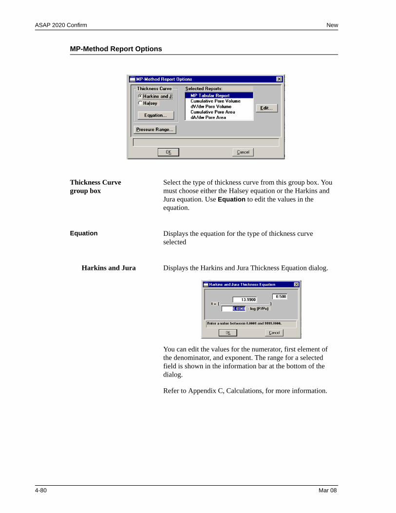
ASAP 2020 Confirm New
MP-Method Report Options
Thickness Curve group box
Select the type of thickness curve from this group box. You must choose either the Halsey equation or the Harkins and Jura equation. Use Equation to edit the values in the equation.
Equation Displays the equation for the type of thickness curve selected
Harkins and Jura Displays the Harkins and Jura Thickness Equation dialog.
You can edit the values for the numerator, first element of the denominator, and exponent. The range for a selected field is shown in the information bar at the bottom of the dialog.
Refer to Appendix C, Calculations, for more information.
4-80 Mar 08
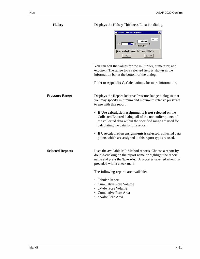
New ASAP 2020 Confirm
Halsey Displays the Halsey Thickness Equation dialog.
You can edit the values for the multiplier, numerator, and exponent.The range for a selected field is shown in the information bar at the bottom of the dialog.
Refer to Appendix C, Calculations, for more information.
Pressure Range Displays the Report Relative Pressure Range dialog so that you may specify minimum and maximum relative pressures to use with this report.
• If Use calculation assignments is not selected on the Collected/Entered dialog, all of the nonoutlier points of the collected data within the specified range are used for calculating the data for this report.
• If Use calculation assignments is selected, collected data points which are assigned to this report type are used.
Selected Reports Lists the available MP-Method reports. Choose a report by double-clicking on the report name or highlight the report name and press the Spacebar. A report is selected when it is preceded with a check mark.
The following reports are available:
• Tabular Report • Cumulative Pore Volume• dV/dw Pore Volume • Cumulative Pore Area• dA/dw Pore Area
Mar 08 4-81
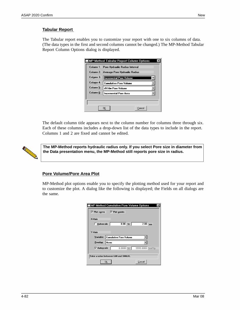
ASAP 2020 Confirm New
Tabular Report
The Tabular report enables you to customize your report with one to six columns of data. (The data types in the first and second columns cannot be changed.) The MP-Method Tabular Report Column Options dialog is displayed.
The default column title appears next to the column number for columns three through six. Each of these columns includes a drop-down list of the data types to include in the report. Columns 1 and 2 are fixed and cannot be edited.
Pore Volume/Pore Area Plot
MP-Method plot options enable you to specify the plotting method used for your report and to customize the plot. A dialog like the following is displayed; the Fields on all dialogs are the same.
The MP-Method reports hydraulic radius only. If you select Pore size in diameter from the Data presentation menu, the MP-Method still reports pore size in radius.
4-82 Mar 08
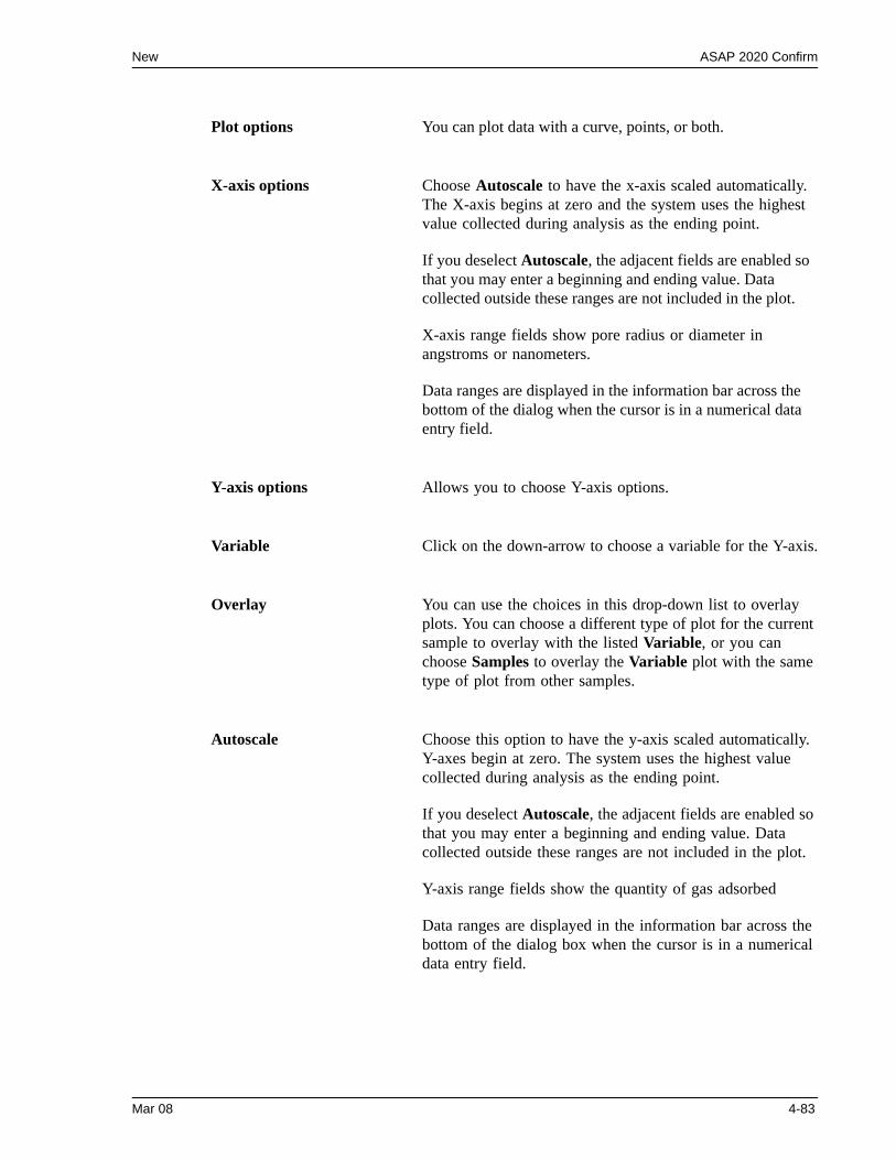
New ASAP 2020 Confirm
Plot options You can plot data with a curve, points, or both.
X-axis options Choose Autoscale to have the x-axis scaled automatically. The X-axis begins at zero and the system uses the highest value collected during analysis as the ending point.
If you deselect Autoscale, the adjacent fields are enabled so that you may enter a beginning and ending value. Data collected outside these ranges are not included in the plot.
X-axis range fields show pore radius or diameter in angstroms or nanometers.
Data ranges are displayed in the information bar across the bottom of the dialog when the cursor is in a numerical data entry field.
Y-axis options Allows you to choose Y-axis options.
Variable Click on the down-arrow to choose a variable for the Y-axis.
Overlay You can use the choices in this drop-down list to overlay plots. You can choose a different type of plot for the current sample to overlay with the listed Variable, or you can choose Samples to overlay the Variable plot with the same type of plot from other samples.
Autoscale Choose this option to have the y-axis scaled automatically. Y-axes begin at zero. The system uses the highest value collected during analysis as the ending point.
If you deselect Autoscale, the adjacent fields are enabled so that you may enter a beginning and ending value. Data collected outside these ranges are not included in the plot.
Y-axis range fields show the quantity of gas adsorbed
Data ranges are displayed in the information bar across the bottom of the dialog box when the cursor is in a numerical data entry field.
Mar 08 4-83
ASAP 2020 Confirm New
Options Report
The Options report is a subset of the contents report; it provides pertinent information for the following:
• Degas conditions• Adsorptive properties• Analysis conditions• Sample tube criteria• Free space• Po and temperature• Equilibration• Isotherm collection
Sample Log Report
The Sample Log report displays the following:
• Manual control operations performed during analysis• Information entered using Add Log Entry on the sample file editor• Warnings and/or errors which occurred during analysis
The Sample Log report is a new feature with the ASAP 2020 program. Therefore, if you request a Sample Log report on a file that was used with the ASAP 2010 program, no information will be available.
4-84 Mar 08
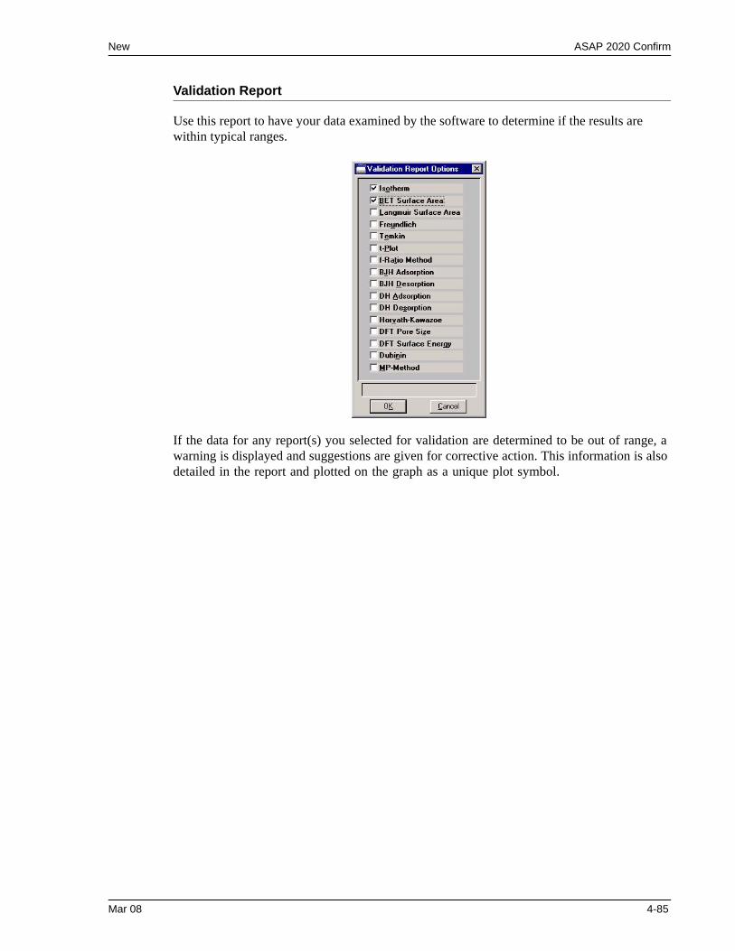
New ASAP 2020 Confirm
Validation Report
Use this report to have your data examined by the software to determine if the results are within typical ranges.
If the data for any report(s) you selected for validation are determined to be out of range, a warning is displayed and suggestions are given for corrective action. This information is also detailed in the report and plotted on the graph as a unique plot symbol.
Mar 08 4-85
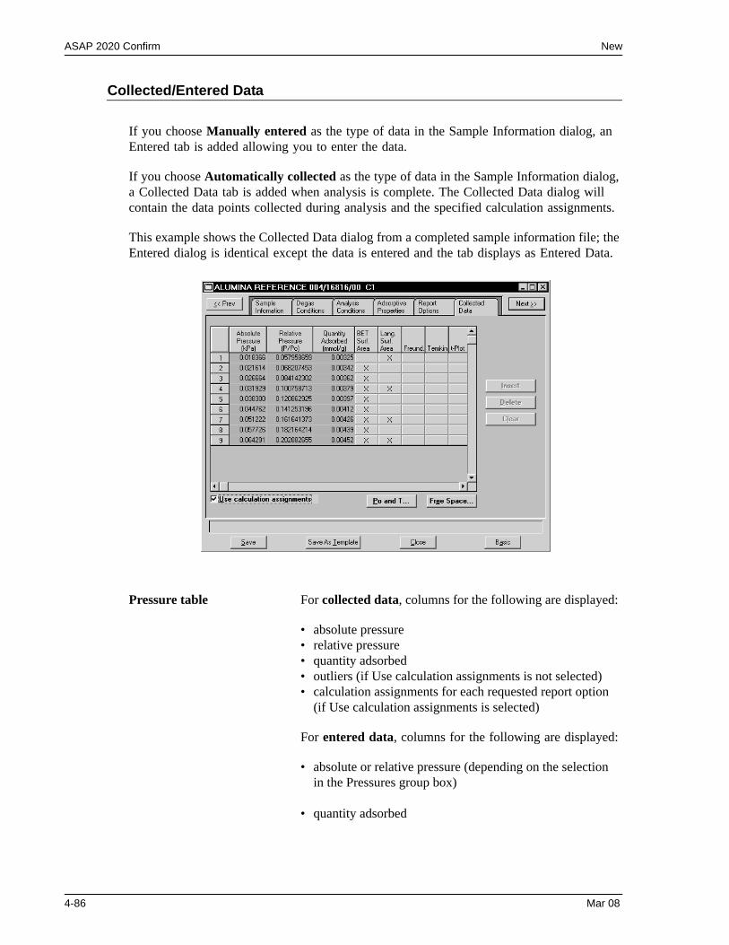
ASAP 2020 Confirm New
Collected/Entered Data
If you choose Manually entered as the type of data in the Sample Information dialog, an Entered tab is added allowing you to enter the data.
If you choose Automatically collected as the type of data in the Sample Information dialog, a Collected Data tab is added when analysis is complete. The Collected Data dialog will contain the data points collected during analysis and the specified calculation assignments.
This example shows the Collected Data dialog from a completed sample information file; the Entered dialog is identical except the data is entered and the tab displays as Entered Data.
Pressure table For collected data, columns for the following are displayed:
• absolute pressure• relative pressure• quantity adsorbed• outliers (if Use calculation assignments is not selected)• calculation assignments for each requested report option
(if Use calculation assignments is selected)
For entered data, columns for the following are displayed:
• absolute or relative pressure (depending on the selection in the Pressures group box)
• quantity adsorbed
4-86 Mar 08
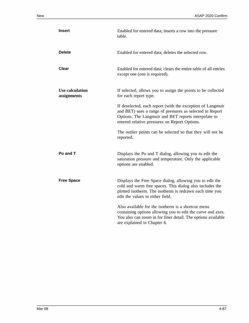
New ASAP 2020 Confirm
Insert Enabled for entered data; inserts a row into the pressure table.
Delete Enabled for entered data; deletes the selected row.
Clear Enabled for entered data; clears the entire table of all entries except one (one is required).
Use calculationassignments
If selected, allows you to assign the points to be collected for each report type.
If deselected, each report (with the exception of Langmuir and BET) uses a range of pressures as selected in Report Options. The Langmuir and BET reports interpolate to entered relative pressures on Report Options.
The outlier points can be selected so that they will not be reported.
Po and T Displays the Po and T dialog, allowing you to edit the saturation pressure and temperature. Only the applicable options are enabled.
Free Space Displays the Free Space dialog, allowing you to edit the cold and warm free spaces. This dialog also includes the plotted isotherm. The isotherm is redrawn each time you edit the values in either field.
Also available for the isotherm is a shortcut menu containing options allowing you to edit the curve and axes. You also can zoom in for finer detail. The options available are explained in Chapter 6.
Mar 08 4-87
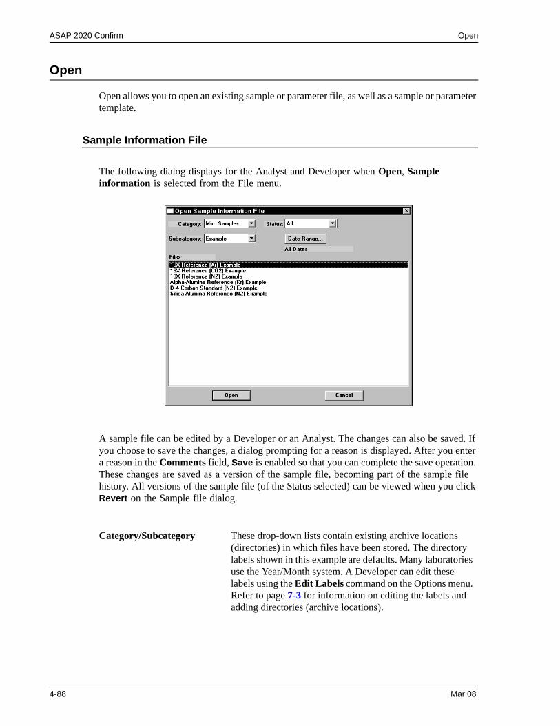
ASAP 2020 Confirm Open
Open
Open allows you to open an existing sample or parameter file, as well as a sample or parameter template.
Sample Information File
The following dialog displays for the Analyst and Developer when Open, Sample information is selected from the File menu.
A sample file can be edited by a Developer or an Analyst. The changes can also be saved. If you choose to save the changes, a dialog prompting for a reason is displayed. After you enter a reason in the Comments field, Save is enabled so that you can complete the save operation. These changes are saved as a version of the sample file, becoming part of the sample file history. All versions of the sample file (of the Status selected) can be viewed when you click Revert on the Sample file dialog.
Category/Subcategory These drop-down lists contain existing archive locations (directories) in which files have been stored. The directory labels shown in this example are defaults. Many laboratories use the Year/Month system. A Developer can edit these labels using the Edit Labels command on the Options menu. Refer to page 7-3 for information on editing the labels and adding directories (archive locations).
4-88 Mar 08
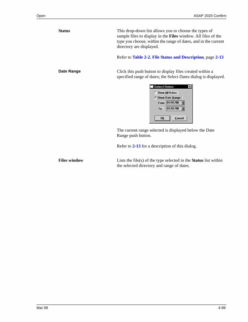
Open ASAP 2020 Confirm
Status This drop-down list allows you to choose the types of sample files to display in the Files window. All files of the type you choose, within the range of dates, and in the current directory are displayed.
Refer to Table 2-2. File Status and Description, page 2-13
Date Range Click this push button to display files created within a specified range of dates; the Select Dates dialog is displayed.
The current range selected is displayed below the Date Range push button.
Refer to 2-13 for a description of this dialog.
Files window Lists the file(s) of the type selected in the Status list within the selected directory and range of dates.
Mar 08 4-89
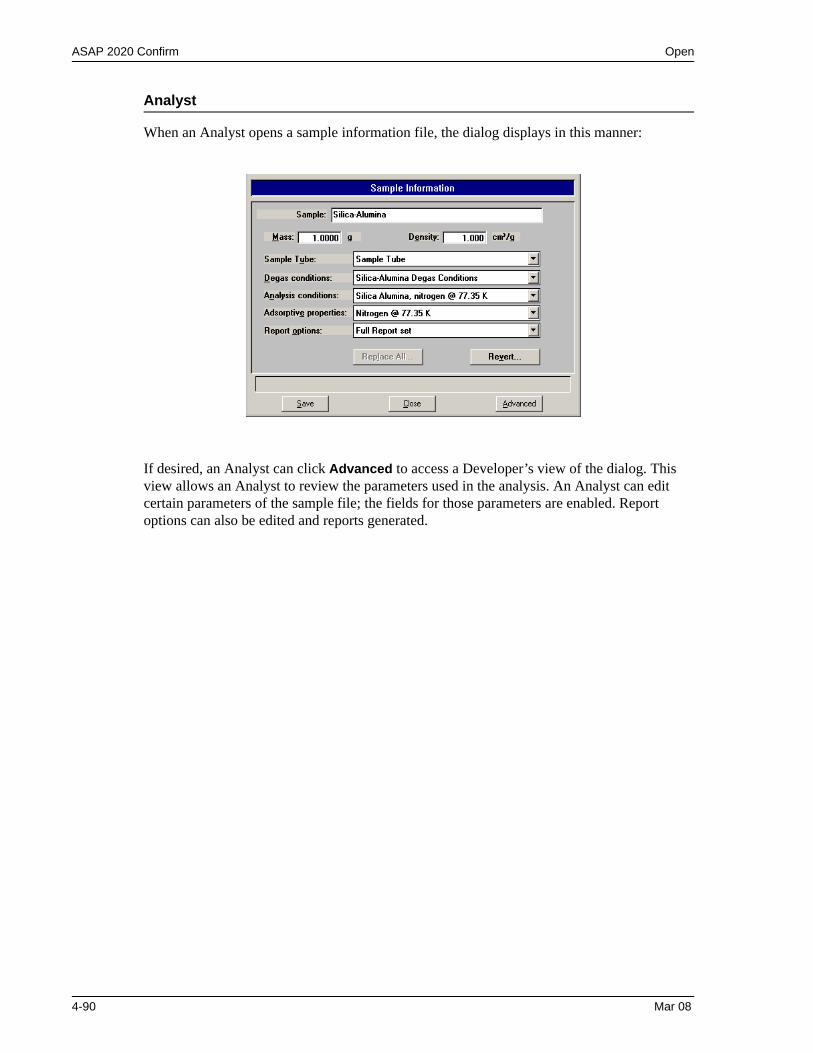
ASAP 2020 Confirm Open
Analyst
When an Analyst opens a sample information file, the dialog displays in this manner:
If desired, an Analyst can click Advanced to access a Developer’s view of the dialog. This view allows an Analyst to review the parameters used in the analysis. An Analyst can edit certain parameters of the sample file; the fields for those parameters are enabled. Report options can also be edited and reports generated.
4-90 Mar 08
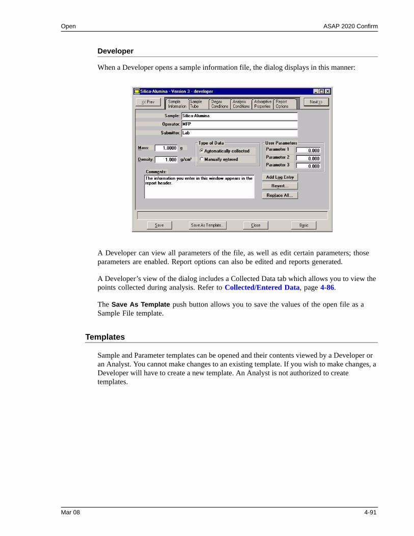
Open ASAP 2020 Confirm
Developer
When a Developer opens a sample information file, the dialog displays in this manner:
A Developer can view all parameters of the file, as well as edit certain parameters; those parameters are enabled. Report options can also be edited and reports generated.
A Developer’s view of the dialog includes a Collected Data tab which allows you to view the points collected during analysis. Refer to Collected/Entered Data, page 4-86.
The Save As Template push button allows you to save the values of the open file as a Sample File template.
Templates
Sample and Parameter templates can be opened and their contents viewed by a Developer or an Analyst. You cannot make changes to an existing template. If you wish to make changes, a Developer will have to create a new template. An Analyst is not authorized to create templates.
Mar 08 4-91
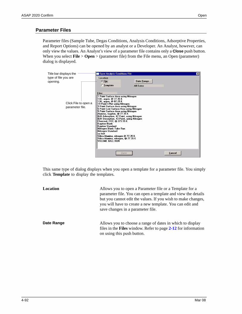
ASAP 2020 Confirm Open
Parameter Files
Parameter files (Sample Tube, Degas Conditions, Analysis Conditions, Adsorptive Properties, and Report Options) can be opened by an analyst or a Developer. An Analyst, however, can only view the values. An Analyst’s view of a parameter file contains only a Close push button. When you select File > Open > (parameter file) from the File menu, an Open (parameter) dialog is displayed.
This same type of dialog displays when you open a template for a parameter file. You simply click Template to display the templates.
Location Allows you to open a Parameter file or a Template for a parameter file. You can open a template and view the details but you cannot edit the values. If you wish to make changes, you will have to create a new template. You can edit and save changes in a parameter file.
Date Range Allows you to choose a range of dates in which to display files in the Files window. Refer to page 2-12 for information on using this push button.
Title bar displays the type of file you are opening.
Click File to open a parameter file.
4-92 Mar 08
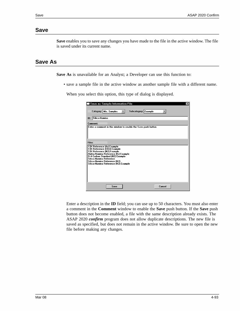
Save ASAP 2020 Confirm
Save
Save enables you to save any changes you have made to the file in the active window. The file is saved under its current name.
Save As
Save As is unavailable for an Analyst; a Developer can use this function to:
• save a sample file in the active window as another sample file with a different name.
When you select this option, this type of dialog is displayed.
Enter a description in the ID field; you can use up to 50 characters. You must also enter a comment in the Comment window to enable the Save push button. If the Save push button does not become enabled, a file with the same description already exists. The ASAP 2020 confirm program does not allow duplicate descriptions. The new file is saved as specified, but does not remain in the active window. Be sure to open the new file before making any changes.
Mar 08 4-93
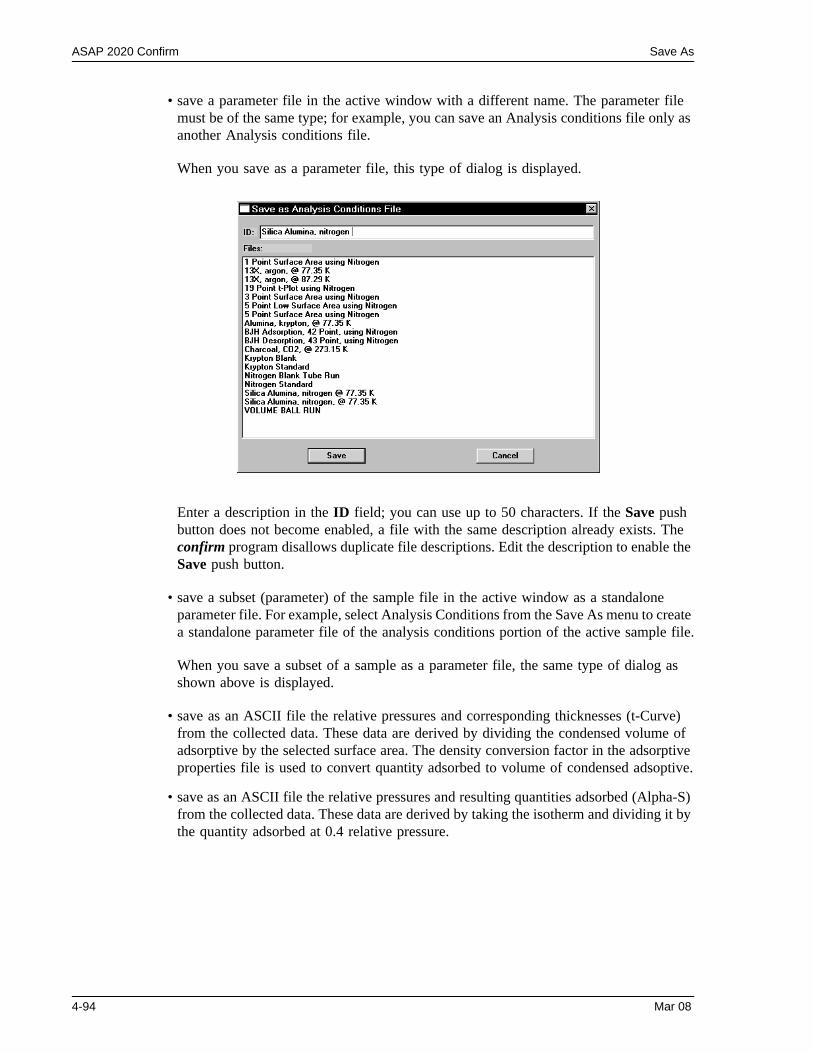
ASAP 2020 Confirm Save As
• save a parameter file in the active window with a different name. The parameter file must be of the same type; for example, you can save an Analysis conditions file only as another Analysis conditions file.
When you save as a parameter file, this type of dialog is displayed.
Enter a description in the ID field; you can use up to 50 characters. If the Save push button does not become enabled, a file with the same description already exists. The confirm program disallows duplicate file descriptions. Edit the description to enable the Save push button.
• save a subset (parameter) of the sample file in the active window as a standalone parameter file. For example, select Analysis Conditions from the Save As menu to create a standalone parameter file of the analysis conditions portion of the active sample file.
When you save a subset of a sample as a parameter file, the same type of dialog as shown above is displayed.
• save as an ASCII file the relative pressures and corresponding thicknesses (t-Curve) from the collected data. These data are derived by dividing the condensed volume of adsorptive by the selected surface area. The density conversion factor in the adsorptive properties file is used to convert quantity adsorbed to volume of condensed adsoptive.
• save as an ASCII file the relative pressures and resulting quantities adsorbed (Alpha-S) from the collected data. These data are derived by taking the isotherm and dividing it by the quantity adsorbed at 0.4 relative pressure.
4-94 Mar 08
Save As Template ASAP 2020 Confirm
Save As Template
Save As Template is unavailable for an Analyst; a Developer can use this function to:
• save the values of the sample file in the active window as a sample template
• save a subset (parameter) of the sample file in the active window as a parameter file template.
• save the values of a parameter file in the active window as a parameter file template.
Save All
Save All enables you to save all open files under their current names. This option provides a faster way to save all open files at one time and avoids having to perform a Save operation on each individual file.
A dialog prompting for a reason for the current change version of each file is displayed.
An Analyst is not authorized to create sample and parameter file templates.
Mar 08 4-95
ASAP 2020 Confirm Close
Close
Close enables you to close the file in the active window. If the file contains changes that have not been saved, the following message is displayed:
(file name) has been changed. Save changes before closing?
Yes No Cancel
Click Yes; a dialog prompting for a reason for the change is displayed before the file closes.
Click No to close the file without saving the changes.
Click Cancel to return to the active file.
Close All
Close All enables you to close all open files under their current names. The following message displays for every file containing changes that have not been saved:
(file name) has been changed. Save changes before closing?
Yes No Cancel
Click Yes; a dialog prompting for a reason for the change is displayed before the file closes.
Click No to close the file without saving the changes.
Click Cancel to return to the active file.
4-96 Mar 08
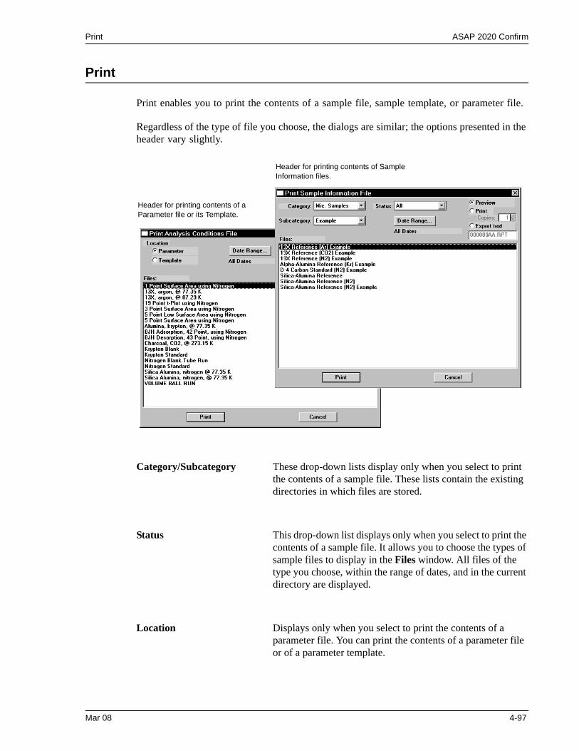
Print ASAP 2020 Confirm
Print enables you to print the contents of a sample file, sample template, or parameter file.
Regardless of the type of file you choose, the dialogs are similar; the options presented in the header vary slightly.
Category/Subcategory These drop-down lists display only when you select to print the contents of a sample file. These lists contain the existing directories in which files are stored.
Status This drop-down list displays only when you select to print the contents of a sample file. It allows you to choose the types of sample files to display in the Files window. All files of the type you choose, within the range of dates, and in the current directory are displayed.
Location Displays only when you select to print the contents of a parameter file. You can print the contents of a parameter file or of a parameter template.
Header for printing contents of Sample Information files.
Header for printing contents of a Parameter file or its Template.
Mar 08 4-97
ASAP 2020 Confirm Print
The remainder of the options display regardless of the type of file you request to print.
Date Range Allows you to specify a range of dates for the files you wish to display in the Files list window, or you can choose All for all files to display. The range you choose is displayed below the push button. (Refer to page 2-12 for an explanation of this push button.)
PreviewPrintExport
Choose Preview to view the file before it is printed; you can then print the file from the preview window.
Choose Print to send the file directly to the printer; you can print up to 4 copies.
Choose Export to print to a file; use the field below the Export option to enter a name. The Export option is unavailable for an Analyst.
Files window Displays the file(s) of the type selected in the Status list within the selected directory and range of dates.You may print the contents of multiple files by holding down Ctrl while selecting files.
4-98 Mar 08
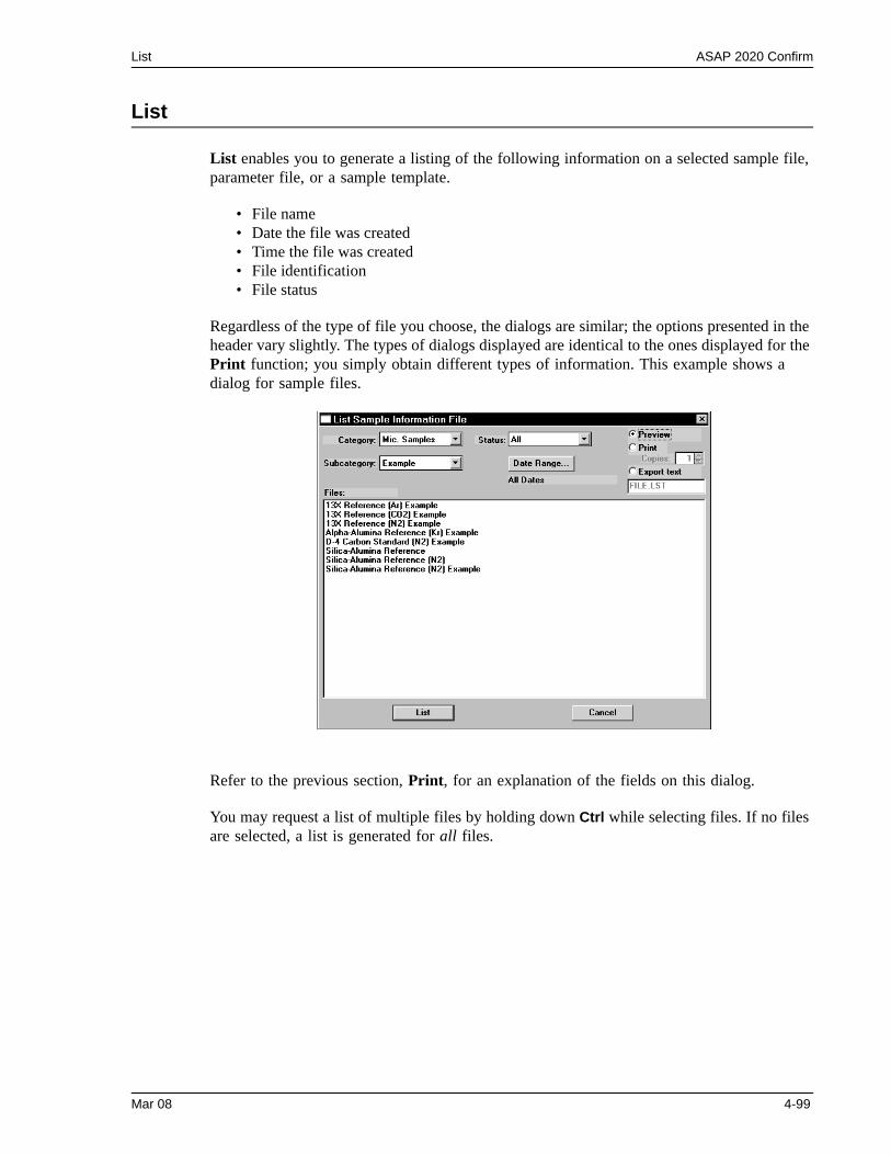
List ASAP 2020 Confirm
List
List enables you to generate a listing of the following information on a selected sample file, parameter file, or a sample template.
• File name• Date the file was created• Time the file was created• File identification• File status
Regardless of the type of file you choose, the dialogs are similar; the options presented in the header vary slightly. The types of dialogs displayed are identical to the ones displayed for the Print function; you simply obtain different types of information. This example shows a dialog for sample files.
Refer to the previous section, Print, for an explanation of the fields on this dialog.
You may request a list of multiple files by holding down Ctrl while selecting files. If no files are selected, a list is generated for all files.
Mar 08 4-99
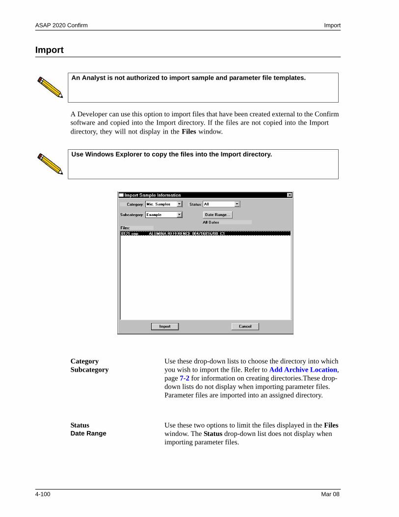
ASAP 2020 Confirm Import
Import
A Developer can use this option to import files that have been created external to the Confirm software and copied into the Import directory. If the files are not copied into the Import directory, they will not display in the Files window.
An Analyst is not authorized to import sample and parameter file templates.
Use Windows Explorer to copy the files into the Import directory.
Category Subcategory
Use these drop-down lists to choose the directory into which you wish to import the file. Refer to Add Archive Location, page 7-2 for information on creating directories.These drop-down lists do not display when importing parameter files. Parameter files are imported into an assigned directory.
StatusDate Range
Use these two options to limit the files displayed in the Files window. The Status drop-down list does not display when importing parameter files.
4-100 Mar 08
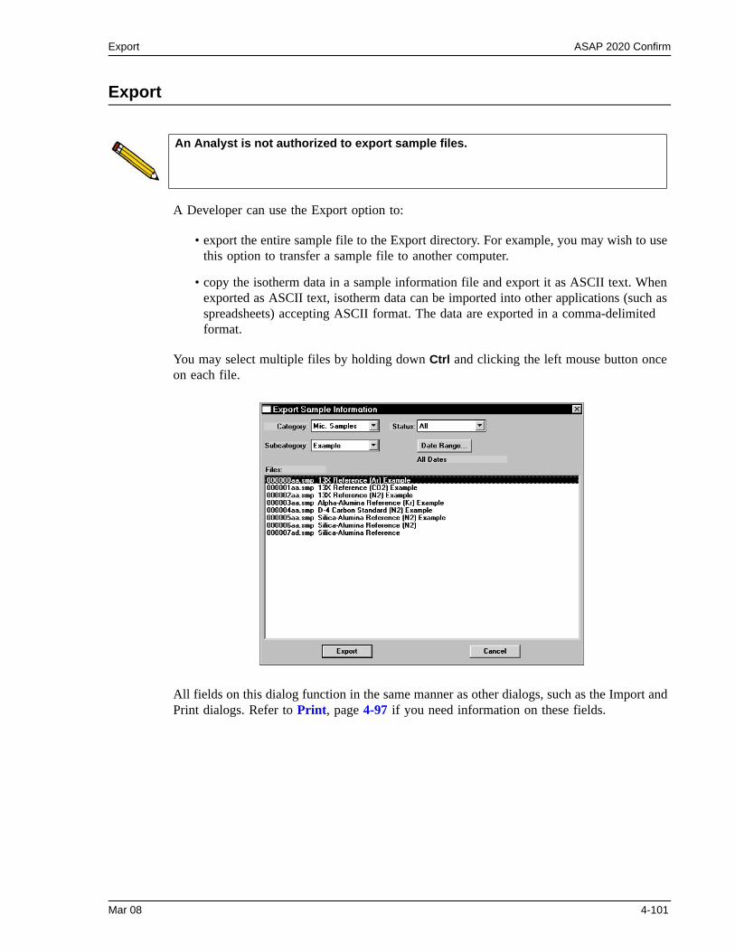
Export ASAP 2020 Confirm
Export
A Developer can use the Export option to:
• export the entire sample file to the Export directory. For example, you may wish to use this option to transfer a sample file to another computer.
• copy the isotherm data in a sample information file and export it as ASCII text. When exported as ASCII text, isotherm data can be imported into other applications (such as spreadsheets) accepting ASCII format. The data are exported in a comma-delimited format.
You may select multiple files by holding down Ctrl and clicking the left mouse button once on each file.
All fields on this dialog function in the same manner as other dialogs, such as the Import and Print dialogs. Refer to Print, page 4-97 if you need information on these fields.
An Analyst is not authorized to export sample files.
Mar 08 4-101
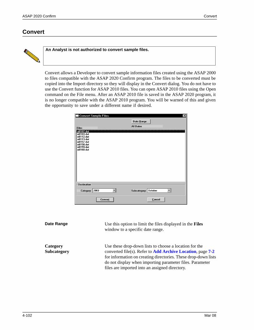
ASAP 2020 Confirm Convert
Convert
Convert allows a Developer to convert sample information files created using the ASAP 2000 to files compatible with the ASAP 2020 Confirm program. The files to be converted must be copied into the Import directory so they will display in the Convert dialog. You do not have to use the Convert function for ASAP 2010 files. You can open ASAP 2010 files using the Open command on the File menu. After an ASAP 2010 file is saved in the ASAP 2020 program, it is no longer compatible with the ASAP 2010 program. You will be warned of this and given the opportunity to save under a different name if desired.
An Analyst is not authorized to convert sample files.
Date Range Use this option to limit the files displayed in the Files window to a specific date range.
Category Subcategory
Use these drop-down lists to choose a location for the converted file(s). Refer to Add Archive Location, page 7-2 for information on creating directories. These drop-down lists do not display when importing parameter files. Parameter files are imported into an assigned directory.
4-102 Mar 08
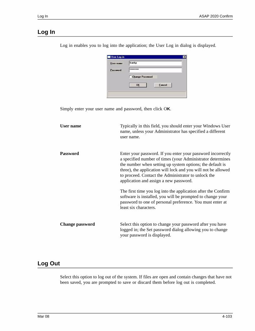
Log In ASAP 2020 Confirm
Log In
Log in enables you to log into the application; the User Log in dialog is displayed.
Simply enter your user name and password, then click OK.
Log Out
Select this option to log out of the system. If files are open and contain changes that have not been saved, you are prompted to save or discard them before log out is completed.
User name Typically in this field, you should enter your Windows User name, unless your Administrator has specified a different user name.
Password Enter your password. If you enter your password incorrectly a specified number of times (your Administrator determines the number when setting up system options; the default is three), the application will lock and you will not be allowed to proceed. Contact the Administrator to unlock the application and assign a new password.
The first time you log into the application after the Confirm software is installed, you will be prompted to change your password to one of personal preference. You must enter at least six characters.
Change password Select this option to change your password after you have logged in; the Set password dialog allowing you to change your password is displayed.
Mar 08 4-103
ASAP 2020 Confirm Exit
Exit
Exit enables you to exit (close) the ASAP 2020 confirm program.
• If a window containing a modified file is open, the following message is displayed:
(file name) has been changed. Save changes before closing?
Yes No Cancel
Click Yes; a dialog prompting for a reason for the change is displayed before the file closes.
Click No to close the file without saving the changes.
Click Cancel to return to the active file.
• If an analysis is in progress, the following message is displayed:
2459- An analyzer is busy. A delay in restarting this application could result in loss of new data. continue with program exit?
Yes No
Click Yes to exit the analysis program but the analysis will continue until completion; analysis data are collected and stored in the analyzer’s memory.
Click No to allow the analysis program to remain active and the analysis to finish
• If a report is in progress, you are cautioned that reports are being generated, and given the opportunity to either cancel the print job or allow the reports to print before exiting.
Although data are stored in the analyzer when you exit the program during analysis, they are not saved in the file until the program is restarted. At that time the data are saved automatically. If a power failure occurs in the interim and you do not have an Uninterruptible Power Supply (UPS) attached, loss of data will result.
4-104 Mar 08
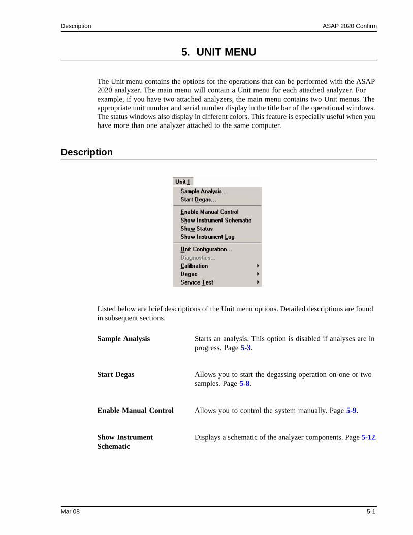
Description ASAP 2020 Confirm
5. UNIT MENU
The Unit menu contains the options for the operations that can be performed with the ASAP 2020 analyzer. The main menu will contain a Unit menu for each attached analyzer. For example, if you have two attached analyzers, the main menu contains two Unit menus. The appropriate unit number and serial number display in the title bar of the operational windows. The status windows also display in different colors. This feature is especially useful when you have more than one analyzer attached to the same computer.
Description
Listed below are brief descriptions of the Unit menu options. Detailed descriptions are found in subsequent sections.
Sample Analysis Starts an analysis. This option is disabled if analyses are in progress. Page 5-3.
Start Degas Allows you to start the degassing operation on one or two samples. Page 5-8.
Enable Manual Control Allows you to control the system manually. Page 5-9.
Show Instrument Schematic
Displays a schematic of the analyzer components. Page 5-12.
Mar 08 5-1
ASAP 2020 Confirm Description
Show Status Shows the status window of the operation in progress. Page 5-13.
Show Instrument Log Displays a log of recent analyses, calibrations, and error mes-sages. Page 5-14.
Unit Configuration Displays the configuration of the analyzer. Page 5-16.
Diagnostics Enables you to perform certain diagnostic tests. Page 5-18
Calibration Enables you to calibrate certain components of the analyzer. Page 5-19.
Degas Allows you to perform sample degassing operations. Enabled only if the SmartVac is installed. Page 5-24.
Service Test Enables you to perform certain troubleshooting procedures. This option is enabled only with the direction of a Micromer-itics service representative. Page 5-29.
5-2 Mar 08
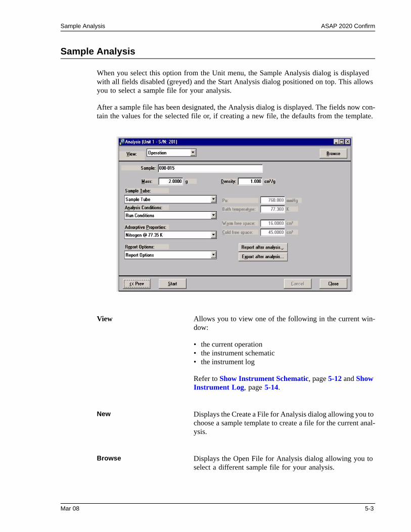
Sample Analysis ASAP 2020 Confirm
Sample Analysis
When you select this option from the Unit menu, the Sample Analysis dialog is displayed with all fields disabled (greyed) and the Start Analysis dialog positioned on top. This allows you to select a sample file for your analysis.
After a sample file has been designated, the Analysis dialog is displayed. The fields now con-tain the values for the selected file or, if creating a new file, the defaults from the template.
View Allows you to view one of the following in the current win-
dow:
• the current operation• the instrument schematic• the instrument log
Refer to Show Instrument Schematic, page 5-12 and Show Instrument Log, page 5-14.
New Displays the Create a File for Analysis dialog allowing you to choose a sample template to create a file for the current anal-ysis.
Browse Displays the Open File for Analysis dialog allowing you to select a different sample file for your analysis.
Mar 08 5-3
ASAP 2020 Confirm Sample Analysis
Sample Displays an identification of the sample file.
Mass Enables you to enter the sample’s mass.
Sample Tube Displays the description of the Sample Tube file for the cur-rent sample file.
The drop-down list contains a list of predefined parameter files. You may choose a different file from this list if desired.
Analysis Conditions Displays the description of the Analysis Conditions file for the current sample file.
The drop-down list contains a list of predefined parameter files. You may choose a different file from this list if desired.
Adsorptive Properties Displays the description of the Adsorptive Properties file for the current sample file.
The drop-down list contains a list of predefined parameter files. You may choose a different file from this list if desired.
Report Options Displays the description of the Report Options file for the current sample file.
The drop-down list contains a list of predefined parameter files. You may choose a different file from this list if desired.
Po Enabled if you have chosen to enter the Po measurement. Enter (or confirm) the saturation pressure of the adsorptive, or edit the current one if desired.
Bath temperature Enabled if you have chosen to enter the bath temperature (Po and T option on the Analysis Conditions dialog). Enter (or confirm) the temperature for the analysis bath.
Warm and Cold Free space Enabled if you have chosen to enter the free space values (Free Space option on the Analysis Conditions dialog). Enter (or confirm) the appropriate value(s).
5-4 Mar 08
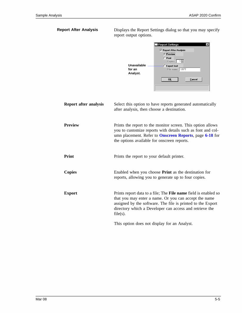
Sample Analysis ASAP 2020 Confirm
Report After Analysis Displays the Report Settings dialog so that you may specify report output options.
Report after analysis Select this option to have reports generated automatically after analysis, then choose a destination.
Preview Prints the report to the monitor screen. This option allows you to customize reports with details such as font and col-umn placement. Refer to Onscreen Reports, page 6-18 for the options available for onscreen reports.
Print Prints the report to your default printer.
Copies Enabled when you choose Print as the destination for reports, allowing you to generate up to four copies.
Export Prints report data to a file; The File name field is enabled so that you may enter a name. Or you can accept the name assigned by the software. The file is printed to the Export directory which a Developer can access and retrieve the file(s).
This option does not display for an Analyst.
Unavailable for an Analyst.
Mar 08 5-5
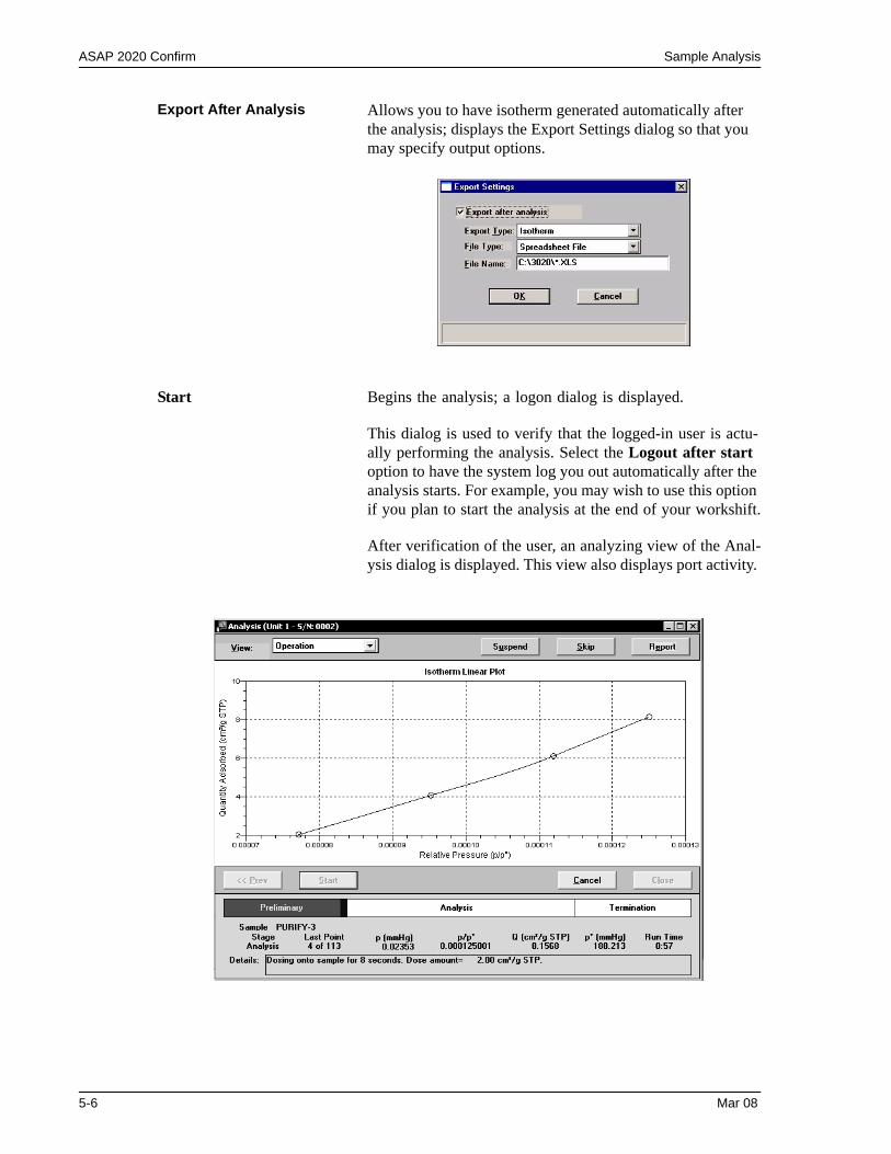
ASAP 2020 Confirm Sample Analysis
Export After Analysis Allows you to have isotherm generated automatically after the analysis; displays the Export Settings dialog so that you may specify output options.
Start Begins the analysis; a logon dialog is displayed.
This dialog is used to verify that the logged-in user is actu-ally performing the analysis. Select the Logout after start option to have the system log you out automatically after the analysis starts. For example, you may wish to use this option if you plan to start the analysis at the end of your workshift.
After verification of the user, an analyzing view of the Anal-ysis dialog is displayed. This view also displays port activity.
5-6 Mar 08
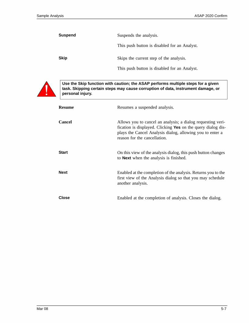
Sample Analysis ASAP 2020 Confirm
Suspend Suspends the analysis.
This push button is disabled for an Analyst.
Skip Skips the current step of the analysis.
This push button is disabled for an Analyst.
Use the Skip function with caution; the ASAP performs multiple steps for a given task. Skipping certain steps may cause corruption of data, instrument damage, or personal injury.
Resume Resumes a suspended analysis.
Cancel Allows you to cancel an analysis; a dialog requesting veri-fication is displayed. Clicking Yes on the query dialog dis-plays the Cancel Analysis dialog, allowing you to enter a reason for the cancellation.
Start On this view of the analysis dialog, this push button changes to Next when the analysis is finished.
Next Enabled at the completion of the analysis. Returns you to the first view of the Analysis dialog so that you may schedule another analysis.
Close Enabled at the completion of analysis. Closes the dialog.
Mar 08 5-7
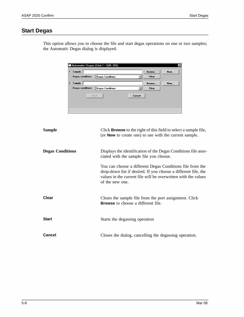
ASAP 2020 Confirm Start Degas
Start Degas
This option allows you to choose the file and start degas operations on one or two samples; the Automatic Degas dialog is displayed.
Sample Click Browse to the right of this field to select a sample file, (or New to create one) to use with the current sample.
Degas Conditions Displays the identification of the Degas Conditions file asso-ciated with the sample file you choose.
You can choose a different Degas Conditions file from the drop-down list if desired. If you choose a different file, the values in the current file will be overwritten with the values of the new one.
Clear Clears the sample file from the port assignment. Click Browse to choose a different file.
Start Starts the degassing operation
Cancel Closes the dialog, cancelling the degassing operation.
5-8 Mar 08
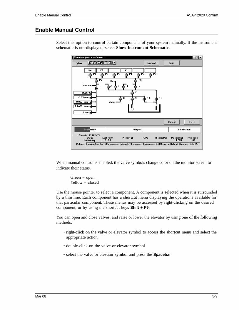
Enable Manual Control ASAP 2020 Confirm
Enable Manual Control
Select this option to control certain components of your system manually. If the instrument schematic is not displayed, select Show Instrument Schematic.
When manual control is enabled, the valve symbols change color on the monitor screen to indicate their status.
Green = openYellow = closed
Use the mouse pointer to select a component. A component is selected when it is surrounded by a thin line. Each component has a shortcut menu displaying the operations available for that particular component. These menus may be accessed by right-clicking on the desired component, or by using the shortcut keys Shift + F9.
You can open and close valves, and raise or lower the elevator by using one of the following methods:
• right-click on the valve or elevator symbol to access the shortcut menu and select the appropriate action
• double-click on the valve or elevator symbol
• select the valve or elevator symbol and press the Spacebar
Mar 08 5-9
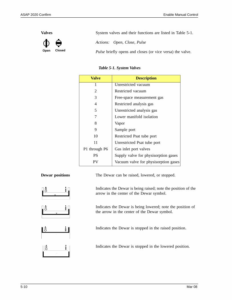
ASAP 2020 Confirm Enable Manual Control
Table 5-1. System Valves
Valves System valves and their functions are listed in Table 5-1.
Actions: Open, Close, Pulse
Pulse briefly opens and closes (or vice versa) the valve.
Valve Description1 Unrestricted vacuum2 Restricted vacuum3 Free-space measurement gas4 Restricted analysis gas5 Unrestricted analysis gas7 Lower manifold isolation8 Vapor9 Sample port
10 Restricted Psat tube port11 Unrestricted Psat tube port
P1 through P6 Gas inlet port valvesPS Supply valve for physisorption gasesPV Vacuum valve for physisorption gases
Dewar positions The Dewar can be raised, lowered, or stopped.
Indicates the Dewar is being raised; note the position of the arrow in the center of the Dewar symbol.
Indicates the Dewar is being lowered; note the position of the arrow in the center of the Dewar symbol.
Indicates the Dewar is stopped in the raised position.
Indicates the Dewar is stopped in the lowered position.
Open Closed
5-10 Mar 08
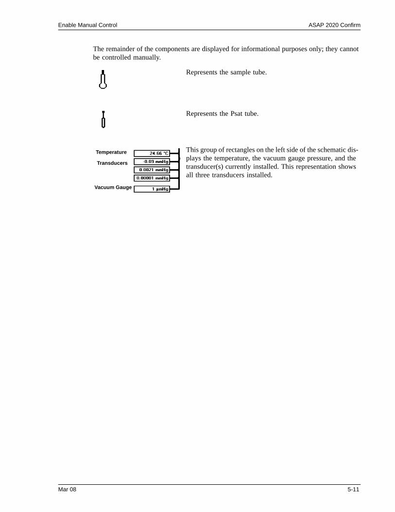
Enable Manual Control ASAP 2020 Confirm
The remainder of the components are displayed for informational purposes only; they cannot be controlled manually.
Represents the sample tube.
Represents the Psat tube.
This group of rectangles on the left side of the schematic dis-plays the temperature, the vacuum gauge pressure, and the transducer(s) currently installed. This representation shows all three transducers installed.
Transducers
Vacuum Gauge
Temperature
Mar 08 5-11
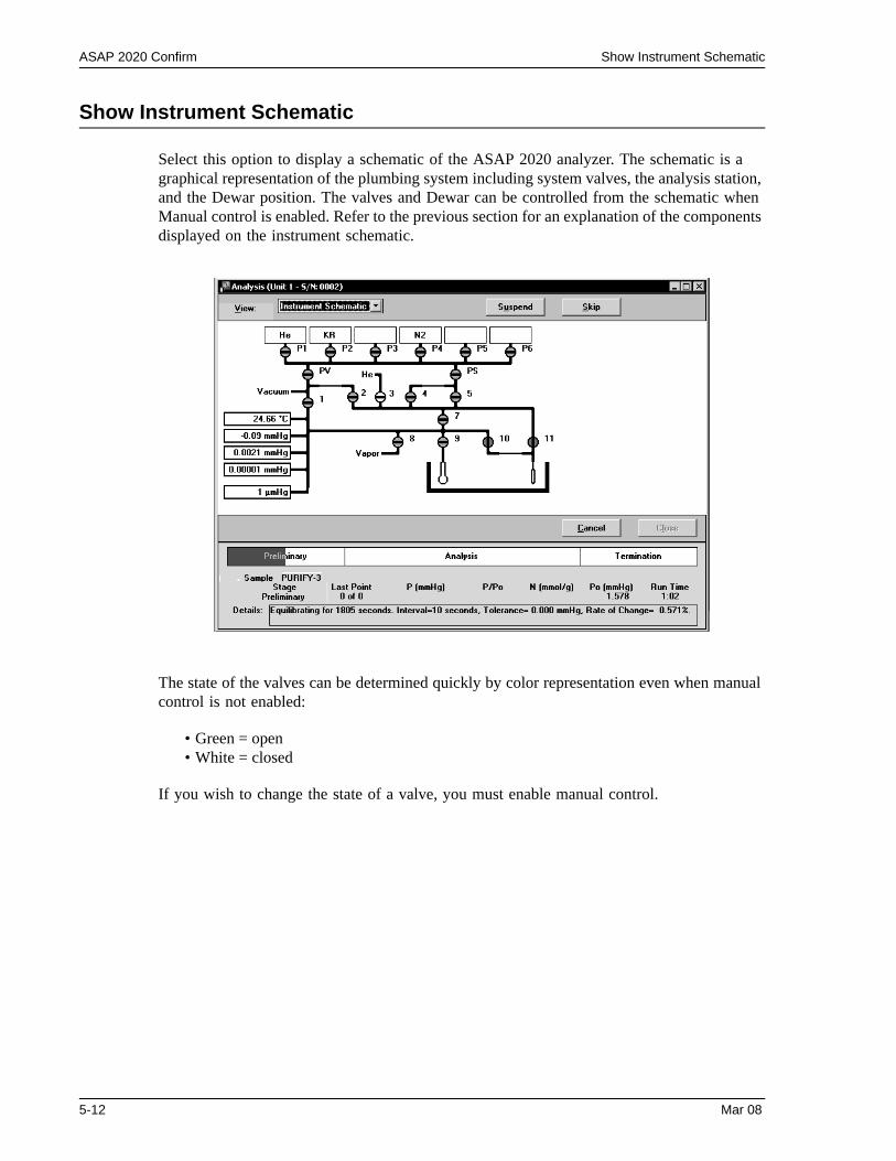
ASAP 2020 Confirm Show Instrument Schematic
Show Instrument Schematic
Select this option to display a schematic of the ASAP 2020 analyzer. The schematic is a graphical representation of the plumbing system including system valves, the analysis station, and the Dewar position. The valves and Dewar can be controlled from the schematic when Manual control is enabled. Refer to the previous section for an explanation of the components displayed on the instrument schematic.
The state of the valves can be determined quickly by color representation even when manual control is not enabled:
• Green = open• White = closed
If you wish to change the state of a valve, you must enable manual control.
5-12 Mar 08
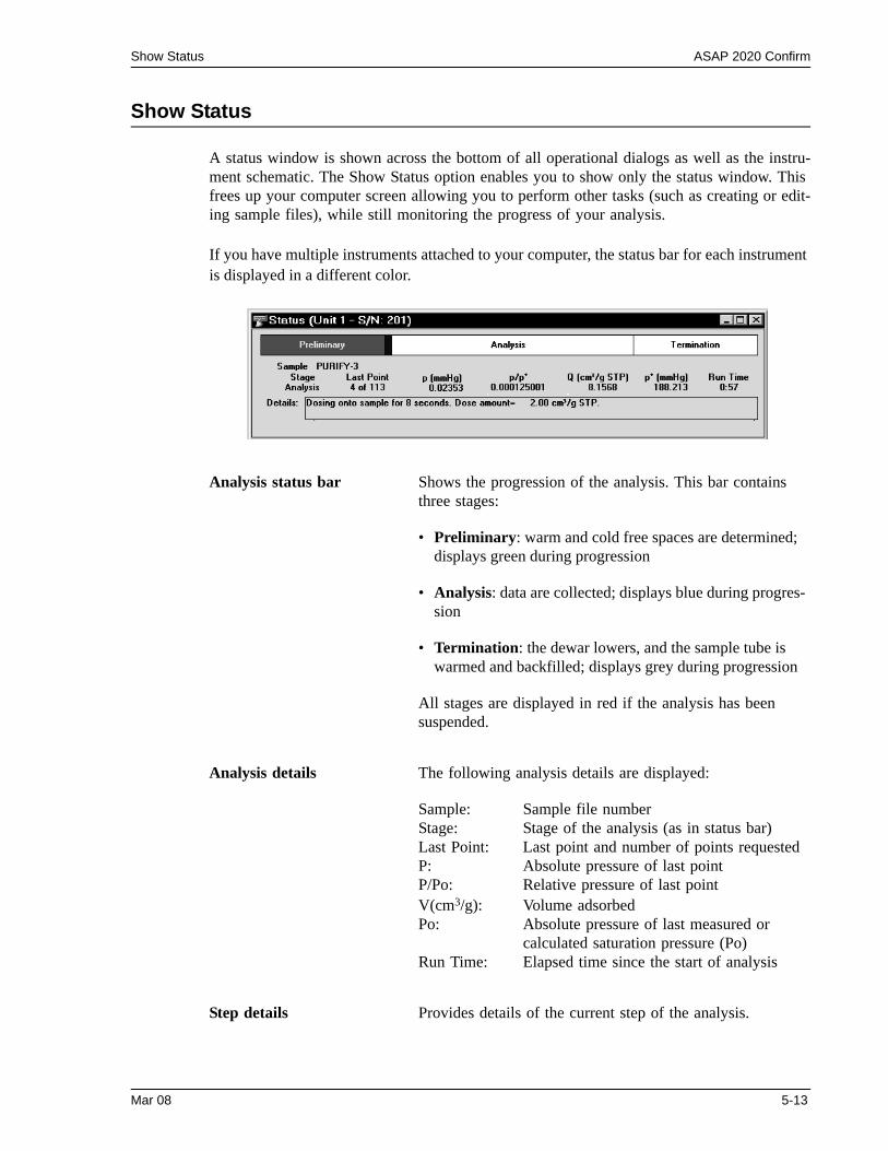
Show Status ASAP 2020 Confirm
Show Status
A status window is shown across the bottom of all operational dialogs as well as the instru-ment schematic. The Show Status option enables you to show only the status window. This frees up your computer screen allowing you to perform other tasks (such as creating or edit-ing sample files), while still monitoring the progress of your analysis.
If you have multiple instruments attached to your computer, the status bar for each instrument is displayed in a different color.
Analysis status bar Shows the progression of the analysis. This bar contains three stages:
• Preliminary: warm and cold free spaces are determined; displays green during progression
• Analysis: data are collected; displays blue during progres-sion
• Termination: the dewar lowers, and the sample tube is warmed and backfilled; displays grey during progression
All stages are displayed in red if the analysis has been suspended.
Analysis details The following analysis details are displayed:
Sample: Sample file numberStage: Stage of the analysis (as in status bar)Last Point: Last point and number of points requestedP: Absolute pressure of last pointP/Po: Relative pressure of last pointV(cm3/g): Volume adsorbedPo: Absolute pressure of last measured or
calculated saturation pressure (Po)Run Time: Elapsed time since the start of analysis
Step details Provides details of the current step of the analysis.
Mar 08 5-13
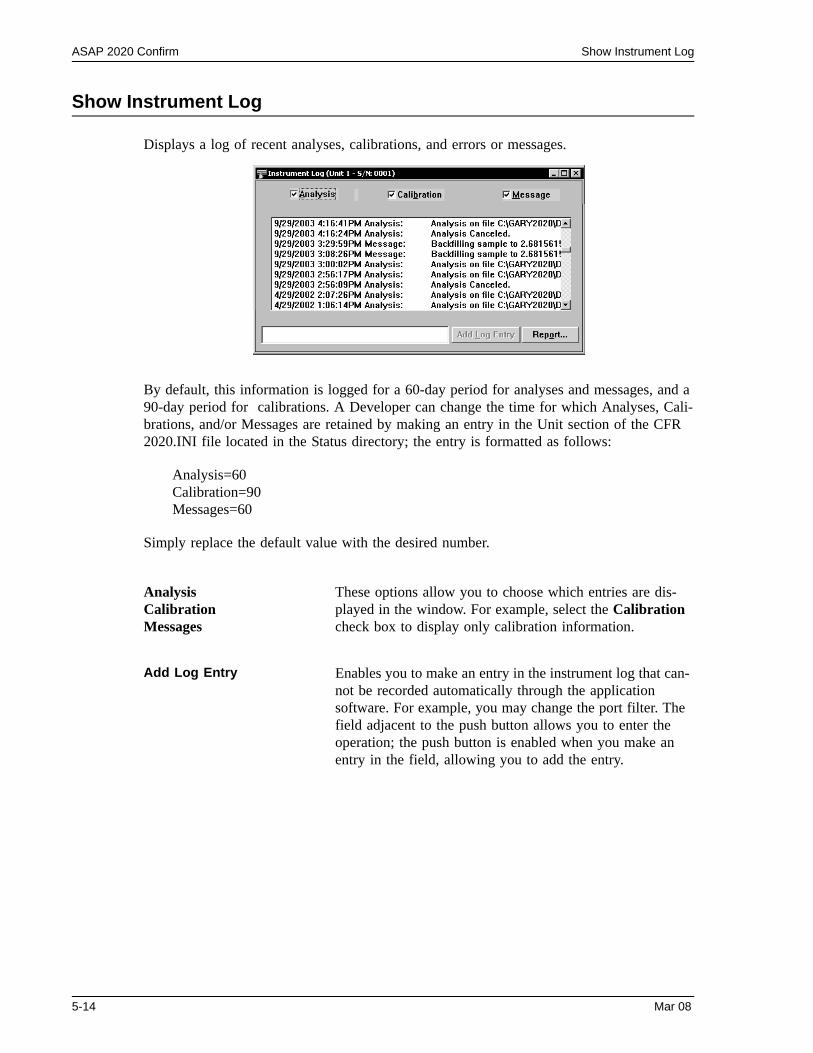
ASAP 2020 Confirm Show Instrument Log
Show Instrument Log
Displays a log of recent analyses, calibrations, and errors or messages.
By default, this information is logged for a 60-day period for analyses and messages, and a 90-day period for calibrations. A Developer can change the time for which Analyses, Cali-brations, and/or Messages are retained by making an entry in the Unit section of the CFR 2020.INI file located in the Status directory; the entry is formatted as follows:
Analysis=60Calibration=90Messages=60
Simply replace the default value with the desired number.
Analysis Calibration Messages
These options allow you to choose which entries are dis-played in the window. For example, select the Calibration check box to display only calibration information.
Add Log Entry Enables you to make an entry in the instrument log that can-not be recorded automatically through the application software. For example, you may change the port filter. The field adjacent to the push button allows you to enter the operation; the push button is enabled when you make an entry in the field, allowing you to add the entry.
5-14 Mar 08
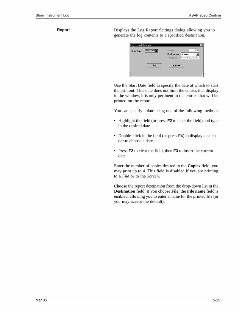
Show Instrument Log ASAP 2020 Confirm
Report Displays the Log Report Settings dialog allowing you to generate the log contents to a specified destination.
Use the Start Date field to specify the date at which to start the printout. This date does not limit the entries that display in the window, it is only pertinent to the entries that will be printed on the report.
You can specify a date using one of the following methods:
• Highlight the field (or press F2 to clear the field) and type in the desired date.
• Double-click in the field (or press F4) to display a calen-dar to choose a date.
• Press F2 to clear the field, then F3 to insert the current date.
Enter the number of copies desired in the Copies field; you may print up to 4. This field is disabled if you are printing to a File or to the Screen.
Choose the report destination from the drop-down list in the Destination field. If you choose File, the File name field is enabled, allowing you to enter a name for the printed file (or you may accept the default).
Mar 08 5-15
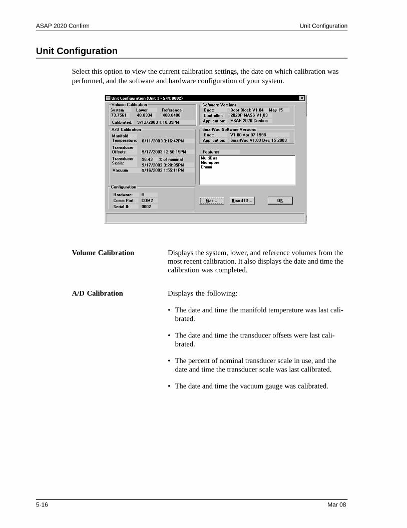
ASAP 2020 Confirm Unit Configuration
Unit Configuration
Select this option to view the current calibration settings, the date on which calibration was performed, and the software and hardware configuration of your system.
Volume Calibration Displays the system, lower, and reference volumes from the most recent calibration. It also displays the date and time the calibration was completed.
A/D Calibration Displays the following:
• The date and time the manifold temperature was last cali-brated.
• The date and time the transducer offsets were last cali-brated.
• The percent of nominal transducer scale in use, and the date and time the transducer scale was last calibrated.
• The date and time the vacuum gauge was calibrated.
5-16 Mar 08
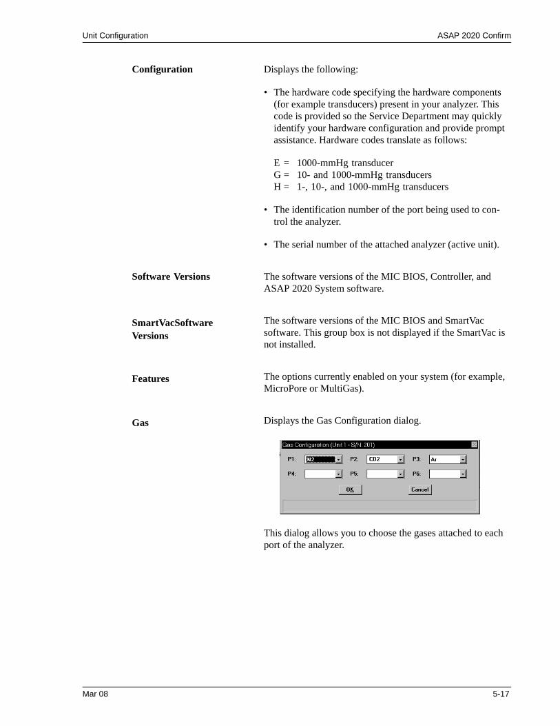
Unit Configuration ASAP 2020 Confirm
Configuration Displays the following:
• The hardware code specifying the hardware components (for example transducers) present in your analyzer. This code is provided so the Service Department may quickly identify your hardware configuration and provide prompt assistance. Hardware codes translate as follows:
E = 1000-mmHg transducerG = 10- and 1000-mmHg transducers H = 1-, 10-, and 1000-mmHg transducers
• The identification number of the port being used to con-trol the analyzer.
• The serial number of the attached analyzer (active unit).
Software Versions The software versions of the MIC BIOS, Controller, and ASAP 2020 System software.
SmartVacSoftware Versions
The software versions of the MIC BIOS and SmartVac software. This group box is not displayed if the SmartVac is not installed.
Features The options currently enabled on your system (for example, MicroPore or MultiGas).
Gas Displays the Gas Configuration dialog.
This dialog allows you to choose the gases attached to each port of the analyzer.
Mar 08 5-17
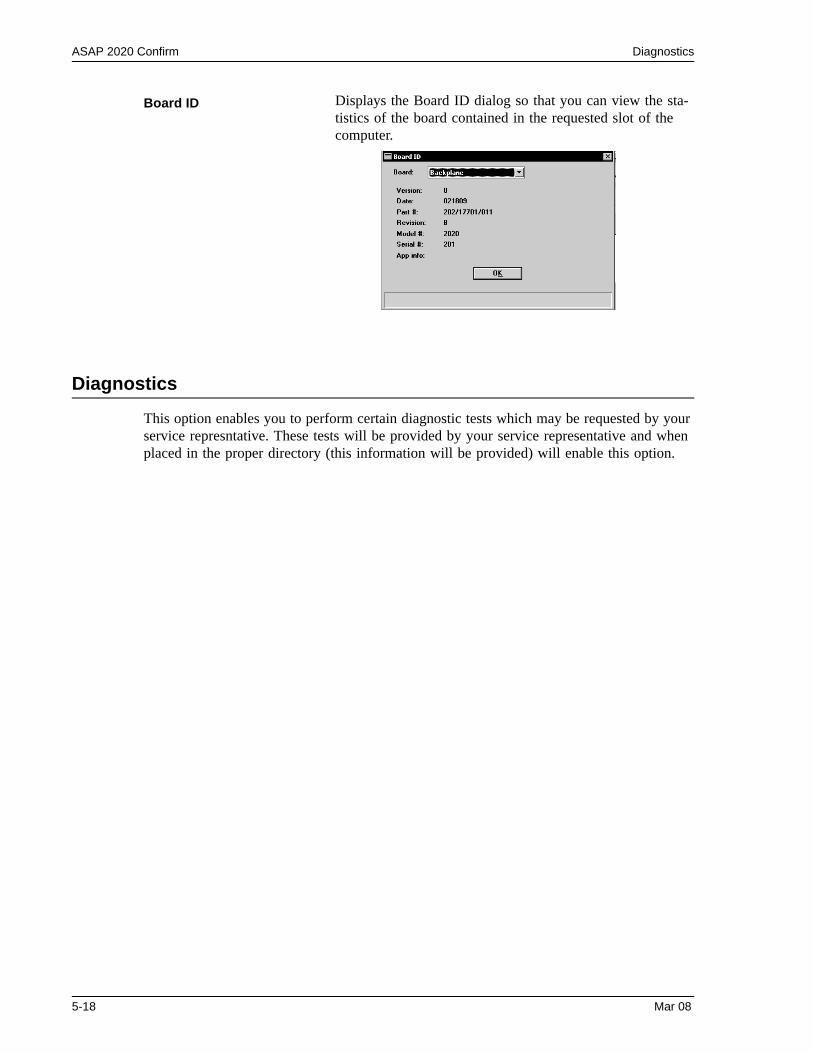
ASAP 2020 Confirm Diagnostics
Diagnostics
This option enables you to perform certain diagnostic tests which may be requested by your service represntative. These tests will be provided by your service representative and when placed in the proper directory (this information will be provided) will enable this option.
Board ID Displays the Board ID dialog so that you can view the sta-tistics of the board contained in the requested slot of the computer.
5-18 Mar 08
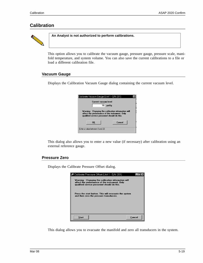
Calibration ASAP 2020 Confirm
Calibration
This option allows you to calibrate the vacuum gauge, pressure gauge, pressure scale, mani-fold temperature, and system volume. You can also save the current calibrations to a file or load a different calibration file.
Vacuum Gauge
Displays the Calibration Vacuum Gauge dialog containing the current vacuum level.
This dialog also allows you to enter a new value (if necessary) after calibration using an external reference gauge.
Pressure Zero
Displays the Calibrate Pressure Offset dialog.
This dialog allows you to evacuate the manifold and zero all transducers in the system.
An Analyst is not authorized to perform calibrations.
Mar 08 5-19
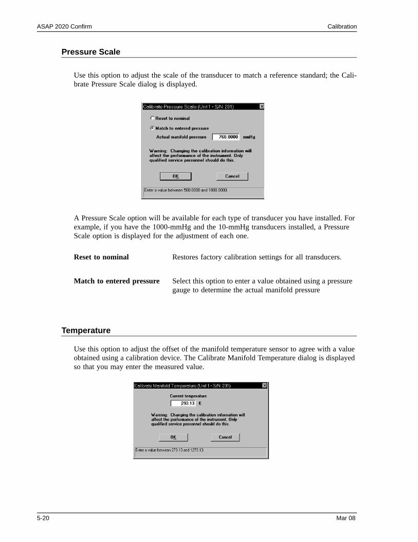
ASAP 2020 Confirm Calibration
Pressure Scale
Use this option to adjust the scale of the transducer to match a reference standard; the Cali-brate Pressure Scale dialog is displayed.
A Pressure Scale option will be available for each type of transducer you have installed. For example, if you have the 1000-mmHg and the 10-mmHg transducers installed, a Pressure Scale option is displayed for the adjustment of each one.
Temperature
Use this option to adjust the offset of the manifold temperature sensor to agree with a value obtained using a calibration device. The Calibrate Manifold Temperature dialog is displayed so that you may enter the measured value.
Reset to nominal Restores factory calibration settings for all transducers.
Match to entered pressure Select this option to enter a value obtained using a pressure gauge to determine the actual manifold pressure
5-20 Mar 08
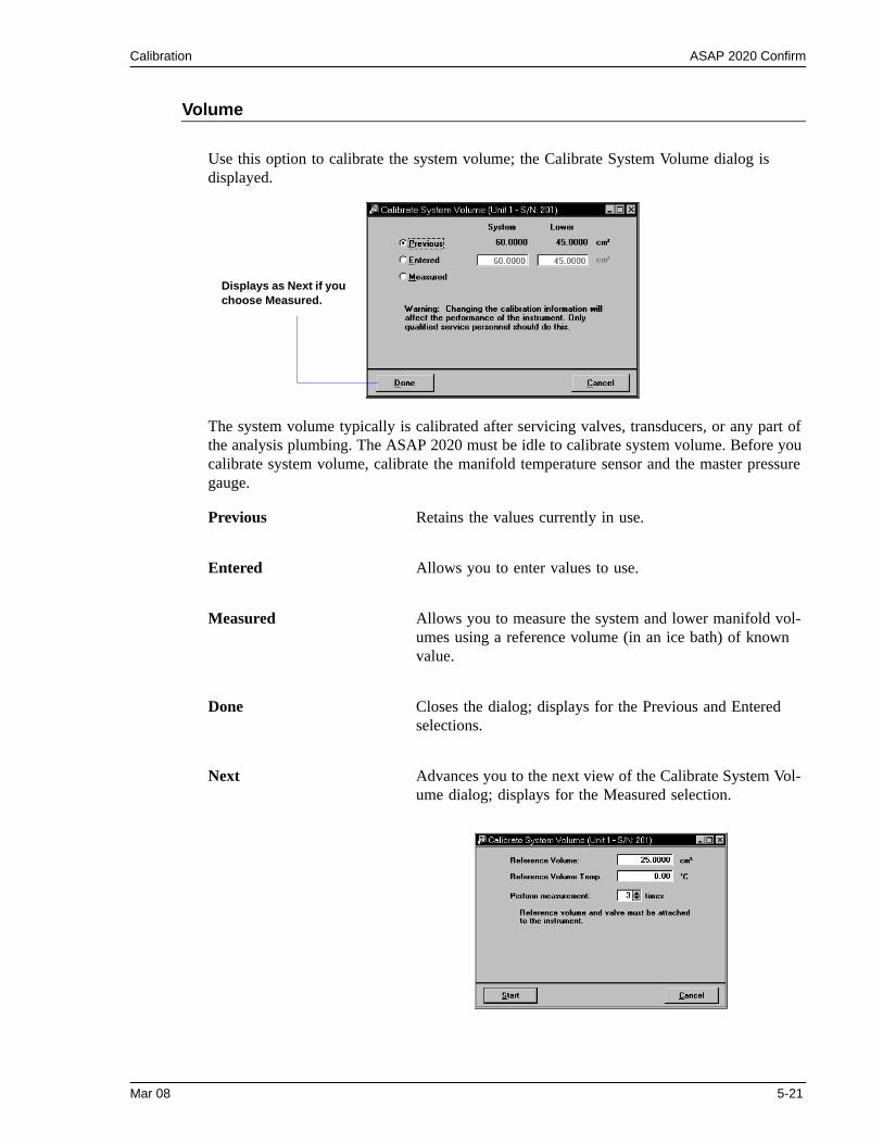
Calibration ASAP 2020 Confirm
Volume
Use this option to calibrate the system volume; the Calibrate System Volume dialog is displayed.
The system volume typically is calibrated after servicing valves, transducers, or any part of the analysis plumbing. The ASAP 2020 must be idle to calibrate system volume. Before you calibrate system volume, calibrate the manifold temperature sensor and the master pressure gauge.
Previous Retains the values currently in use.
Entered Allows you to enter values to use.
Measured Allows you to measure the system and lower manifold vol-umes using a reference volume (in an ice bath) of known value.
Done Closes the dialog; displays for the Previous and Entered selections.
Next Advances you to the next view of the Calibrate System Vol-ume dialog; displays for the Measured selection.
Displays as Next if you choose Measured.
Mar 08 5-21
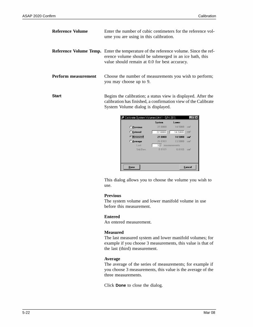
ASAP 2020 Confirm Calibration
Reference Volume Enter the number of cubic centimeters for the reference vol-ume you are using in this calibration.
Reference Volume Temp. Enter the temperature of the reference volume. Since the ref-erence volume should be submerged in an ice bath, this value should remain at 0.0 for best accuracy.
Perform measurement Choose the number of measurements you wish to perform; you may choose up to 9.
Start Begins the calibration; a status view is displayed. After the calibration has finished, a confirmation view of the Calibrate System Volume dialog is displayed.
This dialog allows you to choose the volume you wish to use.
PreviousThe system volume and lower manifold volume in use before this measurement.
EnteredAn entered measurement.
MeasuredThe last measured system and lower manifold volumes; for example if you choose 3 measurements, this value is that of the last (third) measurement.
AverageThe average of the series of measurements; for example if you choose 3 measurements, this value is the average of the three measurements.
Click Done to close the dialog.
5-22 Mar 08
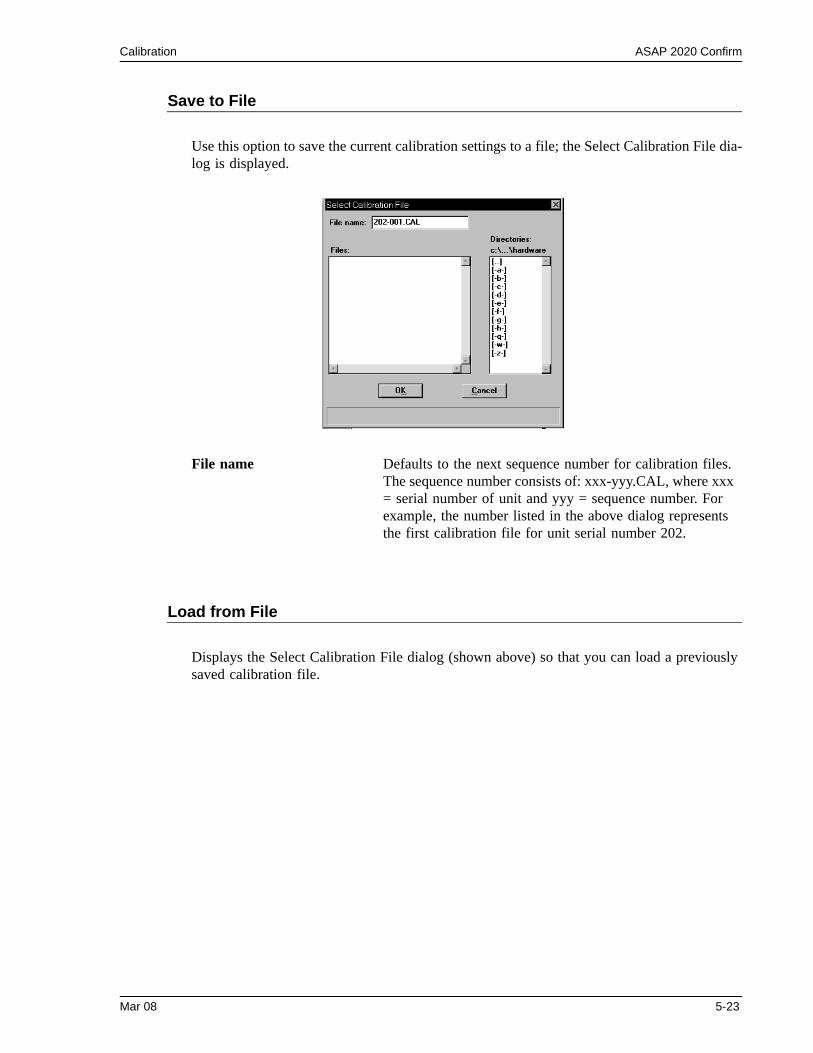
Calibration ASAP 2020 Confirm
Save to File
Use this option to save the current calibration settings to a file; the Select Calibration File dia-log is displayed.
Load from File
Displays the Select Calibration File dialog (shown above) so that you can load a previously saved calibration file.
File name Defaults to the next sequence number for calibration files. The sequence number consists of: xxx-yyy.CAL, where xxx = serial number of unit and yyy = sequence number. For example, the number listed in the above dialog represents the first calibration file for unit serial number 202.
Mar 08 5-23
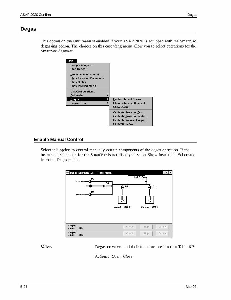
ASAP 2020 Confirm Degas
Degas
This option on the Unit menu is enabled if your ASAP 2020 is equipped with the SmartVac degassing option. The choices on this cascading menu allow you to select operations for the SmartVac degasser.
Enable Manual Control
Select this option to control manually certain components of the degas operation. If the instrument schematic for the SmartVac is not displayed, select Show Instrument Schematic from the Degas menu.
Valves Degasser valves and their functions are listed in Table 6-2.
Actions: Open, Close
5-24 Mar 08
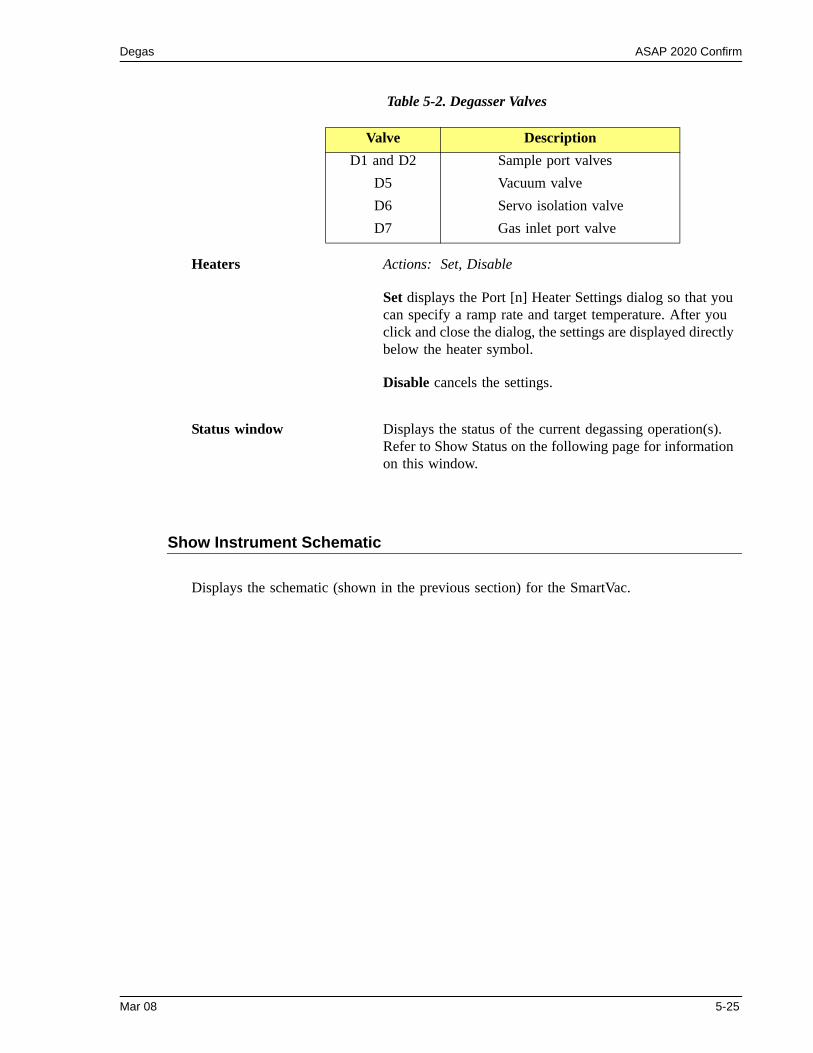
Degas ASAP 2020 Confirm
Table 5-2. Degasser Valves
Show Instrument Schematic
Displays the schematic (shown in the previous section) for the SmartVac.
Valve DescriptionD1 and D2 Sample port valves
D5 Vacuum valveD6 Servo isolation valveD7 Gas inlet port valve
Heaters Actions: Set, Disable
Set displays the Port [n] Heater Settings dialog so that you can specify a ramp rate and target temperature. After you click and close the dialog, the settings are displayed directly below the heater symbol.
Disable cancels the settings.
Status window Displays the status of the current degassing operation(s). Refer to Show Status on the following page for information on this window.
Mar 08 5-25
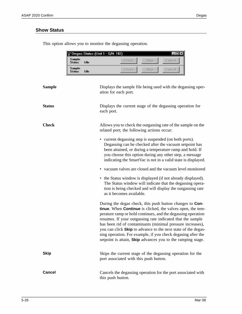
ASAP 2020 Confirm Degas
Show Status
This option allows you to monitor the degassing operation.
Sample Displays the sample file being used with the degassing oper-ation for each port.
Status Displays the current stage of the degassing operation for each port.
Check Allows you to check the outgassing rate of the sample on the related port; the following actions occur:
• current degassing step is suspended (on both ports). Degassing can be checked after the vacuum setpoint has been attained, or during a temperature ramp and hold. If you choose this option during any other step, a message indicating the SmartVac is not in a valid state is displayed.
• vacuum valves are closed and the vacuum level monitored
• the Status window is displayed (if not already displayed). The Status window will indicate that the degassing opera-tion is being checked and will display the outgassing rate as it becomes available.
During the degas check, this push button changes to Con-tinue. When Continue is clicked, the valves open, the tem-perature ramp or hold continues, and the degassing operation resumes. If your outgassing rate indicated that the sample has been rid of contaminants (minimal pressure increases), you can click Skip to advance to the next state of the degas-sing operation. For example, if you check degasing after the setpoint is attain, Skip advances you to the ramping stage.
Skip Skips the current stage of the degassing operation for the port associated with this push button.
Cancel Cancels the degassing operation for the port associated with this push button.
5-26 Mar 08
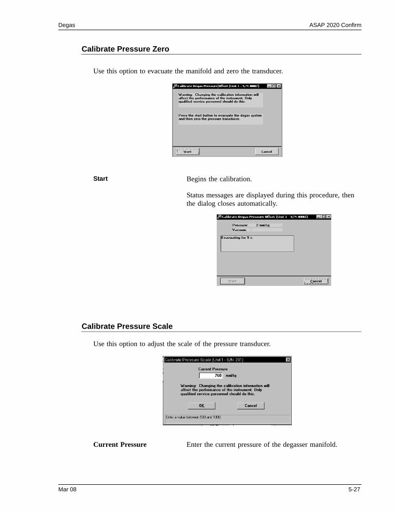
Degas ASAP 2020 Confirm
Calibrate Pressure Zero
Use this option to evacuate the manifold and zero the transducer.
Calibrate Pressure Scale
Use this option to adjust the scale of the pressure transducer.
Start Begins the calibration.
Status messages are displayed during this procedure, then the dialog closes automatically.
Current Pressure Enter the current pressure of the degasser manifold.
Mar 08 5-27
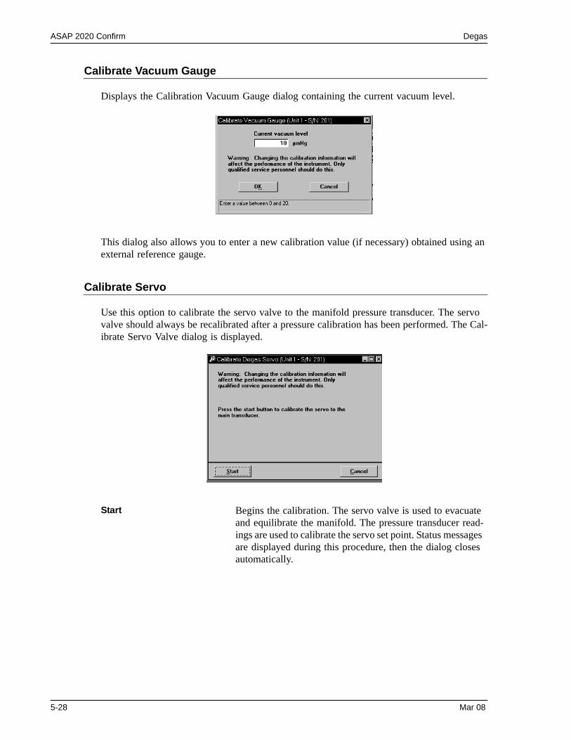
ASAP 2020 Confirm Degas
Calibrate Vacuum Gauge
Displays the Calibration Vacuum Gauge dialog containing the current vacuum level.
This dialog also allows you to enter a new calibration value (if necessary) obtained using an external reference gauge.
Calibrate Servo
Use this option to calibrate the servo valve to the manifold pressure transducer. The servo valve should always be recalibrated after a pressure calibration has been performed. The Cal-ibrate Servo Valve dialog is displayed.
Start Begins the calibration. The servo valve is used to evacuate and equilibrate the manifold. The pressure transducer read-ings are used to calibrate the servo set point. Status messages are displayed during this procedure, then the dialog closes automatically.
5-28 Mar 08

Service Test ASAP 2020 Confirm
Service Test
Various service tests are included in the ASAP 2020 operating program. These tests can be enabled and performed only with the assistance of a trained Micromeritics service represen-tative. These tests are designed to provide your service representative with instrument readouts, as well as to assist him in troubleshooting potential problems and, perhaps, elimi-nating unnecessary repair services. This service strategy allows you to conduct expert tests in less time than it would take to be trained in servicing the instrument properly.
Mar 08 5-29

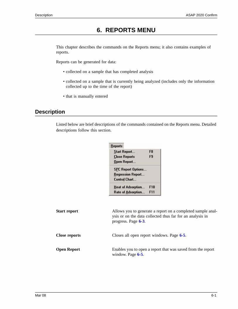
Description ASAP 2020 Confirm
6. REPORTS MENU
This chapter describes the commands on the Reports menu; it also contains examples of reports.
Reports can be generated for data:
• collected on a sample that has completed analysis
• collected on a sample that is currently being analyzed (includes only the information collected up to the time of the report)
• that is manually entered
Description
Listed below are brief descriptions of the commands contained on the Reports menu. Detailed descriptions follow this section.
Start report Allows you to generate a report on a completed sample anal-ysis or on the data collected thus far for an analysis in progress. Page 6-3.
Close reports Closes all open report windows. Page 6-5.
Open Report Enables you to open a report that was saved from the report window. Page 6-5.
Mar 08 6-1
ASAP 2020 Confirm Description
SPC Report Options Allows you to specify the sample data to be included in SPC reports. Page 6-6.
Regression Report Allows you to generate a regression report. Page 6-7.
Control Chart Allows you to generate a control chart report. Page 6-11.
Heat of Adsorption Allows you to generate a Heat of Adsorption report. Page 6-3.
Rate of Adsorption Invokes the Rate of Adsorption program, allowing you to generate ROA reports. Page 6-3.
6-2 Mar 08
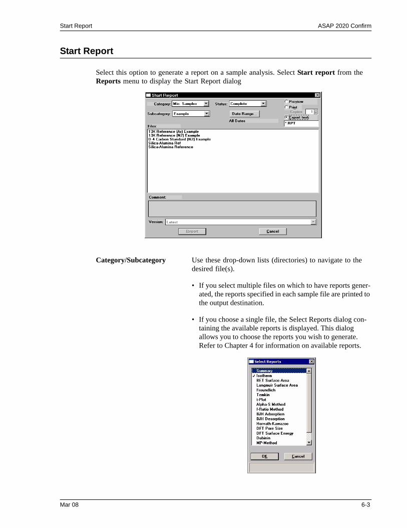
Start Report ASAP 2020 Confirm
Start Report
Select this option to generate a report on a sample analysis. Select Start report from the Reports menu to display the Start Report dialog
Category/Subcategory Use these drop-down lists (directories) to navigate to the desired file(s).
• If you select multiple files on which to have reports gener-ated, the reports specified in each sample file are printed to the output destination.
• If you choose a single file, the Select Reports dialog con-taining the available reports is displayed. This dialog allows you to choose the reports you wish to generate. Refer to Chapter 4 for information on available reports.
Mar 08 6-3
ASAP 2020 Confirm Start Report
Category/Subcategory(continued)
Select (or deselect) reports by double-clicking on the desired report (reports are selected when they are preceded with a check mark). Alternatively, you can highlight the report and press Spacebar.
Status This drop-down list determines what type of sample files are displayed in the Files list window in the specified directory for all dates, or within the specified range of dates (using push button).
Choices: All, Analyzing, Complete, Entered
Refer to Table 2-2. File Status and Description, page 2-13 for a description of the status types.
Date Range Displays the Select Dates dialog so that you may specify a range of dates. Refer to Selecting Files on page 2-12 for a description of this push button.
Preview Choose this option to have the report(s) generated to the screen. If a printed copy is desired, you can print the report from the report window.
Options for customizing and fine-tuning data are available for onscreen reports.
Print Choose this option to have the report(s) generated directly to the printer without reviewing them first. If you choose this option, the Copies field is enabled allowing you to print up to four copies.
Files window Displays a list of the available sample files for the choice shown in the Status field and within the range of dates spec-ified in the Dates dialog.
6-4 Mar 08
Close Reports ASAP 2020 Confirm
Close Reports
This option enables you to close all open report windows at one time. This avoids having to select close on each report window.
Open Report
Enables you to open a report that was saved from the Report window.
Mar 08 6-5
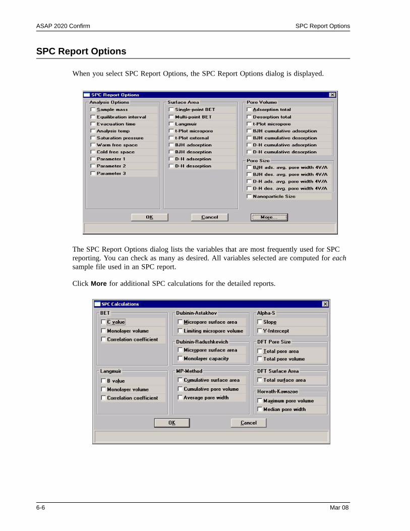
ASAP 2020 Confirm SPC Report Options
SPC Report Options
When you select SPC Report Options, the SPC Report Options dialog is displayed.
The SPC Report Options dialog lists the variables that are most frequently used for SPC reporting. You can check as many as desired. All variables selected are computed for each sample file used in an SPC report.
Click More for additional SPC calculations for the detailed reports.
6-6 Mar 08
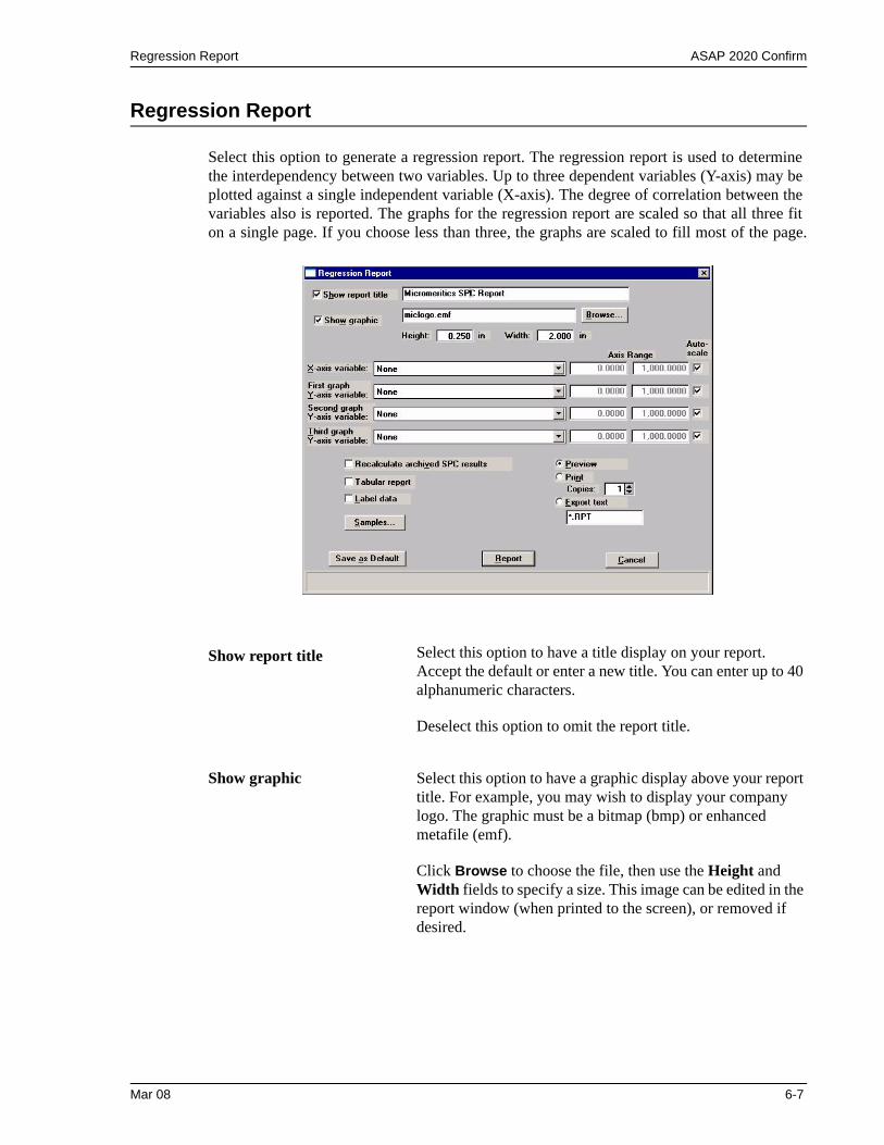
Regression Report ASAP 2020 Confirm
Regression Report
Select this option to generate a regression report. The regression report is used to determine the interdependency between two variables. Up to three dependent variables (Y-axis) may be plotted against a single independent variable (X-axis). The degree of correlation between the variables also is reported. The graphs for the regression report are scaled so that all three fit on a single page. If you choose less than three, the graphs are scaled to fill most of the page.
Show report title Select this option to have a title display on your report. Accept the default or enter a new title. You can enter up to 40 alphanumeric characters.
Deselect this option to omit the report title.
Show graphic Select this option to have a graphic display above your report title. For example, you may wish to display your company logo. The graphic must be a bitmap (bmp) or enhanced metafile (emf).
Click Browse to choose the file, then use the Height and Width fields to specify a size. This image can be edited in the report window (when printed to the screen), or removed if desired.
Mar 08 6-7
ASAP 2020 Confirm Regression Report
X- and Y-Axes Variable fields
Allows you to designate the X- and Y-axes variables. Click on the down arrow to display a list of variables. The variables in this list are the ones you specified in the SPC report options.
With this option, you can plot the regression of up to three Y-axis variables against the X-axis variable. The X-axis specifies the independent variable for the regression, while the Y-axes provide the dependent variables.
Axis Range Enables you to specify the beginning and ending values for the X- and Y-axis ranges. Data collected outside these ranges are not included in the plot. These fields are disabled if you choose Autoscale.
Autoscale Allows you to have the X- and/or Y-axes scaled automatically. When scaled automatically, both axes begin at zero. The analysis program uses the highest values collected during analysis as the ending points.
Recalculate archived SPC results
Select this option to have archived SPC values recalculated. This ensures that any changes made to the SPC Report Options are included in the new report; however, it does lengthen the time required to generate the report.
Tabular report Enables you to generate tabular, as well as graphical, data of the included samples. A tabular report contains the numeric values contributed by each sample.
Label data Allows you to label the points on the plot to correspond with the values in the sample files.
Samples Displays the Regression Report Sample Selection dialog, allowing you to choose the sample files you wish to have reported.
6-8 Mar 08
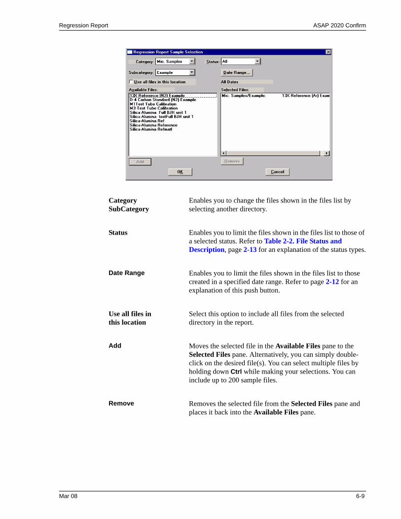
Regression Report ASAP 2020 Confirm
CategorySubCategory
Enables you to change the files shown in the files list by selecting another directory.
Status Enables you to limit the files shown in the files list to those of a selected status. Refer to Table 2-2. File Status and Description, page 2-13 for an explanation of the status types.
Date Range Enables you to limit the files shown in the files list to those created in a specified date range. Refer to page 2-12 for an explanation of this push button.
Use all files inthis location
Select this option to include all files from the selected directory in the report.
Add Moves the selected file in the Available Files pane to the Selected Files pane. Alternatively, you can simply double-click on the desired file(s). You can select multiple files by holding down Ctrl while making your selections. You can include up to 200 sample files.
Remove Removes the selected file from the Selected Files pane and places it back into the Available Files pane.
Mar 08 6-9

ASAP 2020 Confirm Regression Report
PreviewPrintExport text
Enables you to specify the report destination.
The Export options is not available for an Analyst.
Save As Default Saves the current definition of the report as the default.
Report Generates the report.
6-10 Mar 08
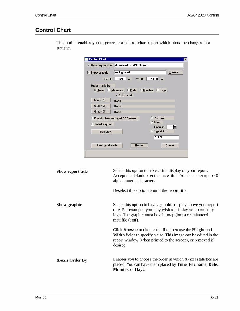
Control Chart ASAP 2020 Confirm
Control Chart
This option enables you to generate a control chart report which plots the changes in a statistic.
Show report title Select this option to have a title display on your report. Accept the default or enter a new title. You can enter up to 40 alphanumeric characters.
Deselect this option to omit the report title.
Show graphic Select this option to have a graphic display above your report title. For example, you may wish to display your company logo. The graphic must be a bitmap (bmp) or enhanced metafile (emf).
Click Browse to choose the file, then use the Height and Width fields to specify a size. This image can be edited in the report window (when printed to the screen), or removed if desired.
X-axis Order By Enables you to choose the order in which X-axis statistics are placed. You can have them placed by Time, File name, Date, Minutes, or Days.
Mar 08 6-11
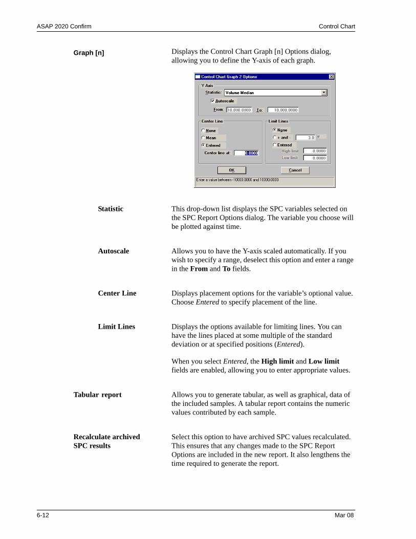
ASAP 2020 Confirm Control Chart
Graph [n] Displays the Control Chart Graph [n] Options dialog, allowing you to define the Y-axis of each graph.
Statistic This drop-down list displays the SPC variables selected on the SPC Report Options dialog. The variable you choose will be plotted against time.
Autoscale Allows you to have the Y-axis scaled automatically. If you wish to specify a range, deselect this option and enter a range in the From and To fields.
Center Line Displays placement options for the variable’s optional value. Choose Entered to specify placement of the line.
Limit Lines Displays the options available for limiting lines. You can have the lines placed at some multiple of the standard deviation or at specified positions (Entered).
When you select Entered, the High limit and Low limit fields are enabled, allowing you to enter appropriate values.
Tabular report Allows you to generate tabular, as well as graphical, data of the included samples. A tabular report contains the numeric values contributed by each sample.
Recalculate archived SPC results
Select this option to have archived SPC values recalculated. This ensures that any changes made to the SPC Report Options are included in the new report. It also lengthens the time required to generate the report.
6-12 Mar 08
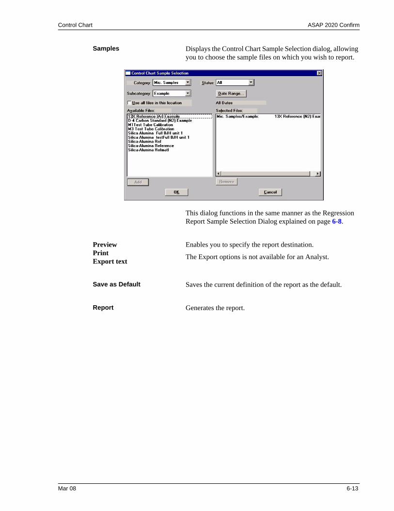
Control Chart ASAP 2020 Confirm
Samples Displays the Control Chart Sample Selection dialog, allowing you to choose the sample files on which you wish to report.
This dialog functions in the same manner as the Regression Report Sample Selection Dialog explained on page 6-8.
PreviewPrintExport text
Enables you to specify the report destination.
The Export options is not available for an Analyst.
Save as Default Saves the current definition of the report as the default.
Report Generates the report.
Mar 08 6-13
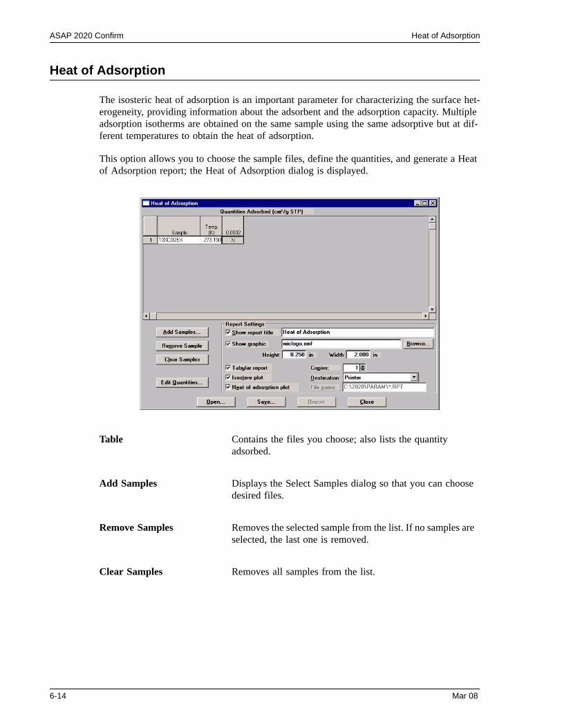
ASAP 2020 Confirm Heat of Adsorption
Heat of Adsorption
The isosteric heat of adsorption is an important parameter for characterizing the surface het-erogeneity, providing information about the adsorbent and the adsorption capacity. Multiple adsorption isotherms are obtained on the same sample using the same adsorptive but at dif-ferent temperatures to obtain the heat of adsorption.
This option allows you to choose the sample files, define the quantities, and generate a Heat of Adsorption report; the Heat of Adsorption dialog is displayed.
Table Contains the files you choose; also lists the quantity adsorbed.
Add Samples Displays the Select Samples dialog so that you can choose desired files.
Remove Samples Removes the selected sample from the list. If no samples are selected, the last one is removed.
Clear Samples Removes all samples from the list.
6-14 Mar 08
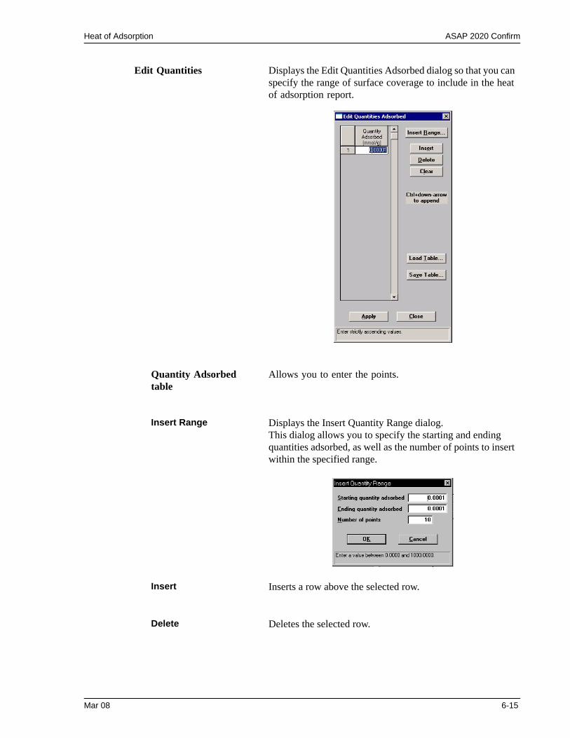
Heat of Adsorption ASAP 2020 Confirm
Edit Quantities Displays the Edit Quantities Adsorbed dialog so that you can specify the range of surface coverage to include in the heat of adsorption report.
Quantity Adsorbed table
Allows you to enter the points.
Insert Range Displays the Insert Quantity Range dialog.This dialog allows you to specify the starting and ending quantities adsorbed, as well as the number of points to insert within the specified range.
Insert Inserts a row above the selected row.
Delete Deletes the selected row.
Mar 08 6-15
ASAP 2020 Confirm Heat of Adsorption
Clear Clears the entire table of all entries except one; one is required.
Load Table Allows you to import a previously saved table.
Save Table Allows you to save the current table as a file (QNT extension).
Apply Applies the quantities in the table to the curent Heat of Adsorption report.
Report Settings The options in this group box allow you to choose report cri-teria
Show report title Choose this option to have a title display in the header of your report, then use the adjacent field to enter the title.
Show graphic This option allows you to have a graphic appear in your title; for example, you may wish to show your company logo. You can use a bitmap or an enhanced metafile.
Use the Height and Width fields to define a size.
Tabular report Select this option to have data generated in a tabular format.
Isostere plot Select this option to generate a graph showing quantities of gas adsorbed vs. the temperature.
Heat of adsorption plot
Select this option to generate the Heat of Adsorption data in a graphical format.
Preview Select this option to print reports to the screen. There are many options for customizing reports onscreen. You can print a hard copy from the report window if desired.
6-16 Mar 08
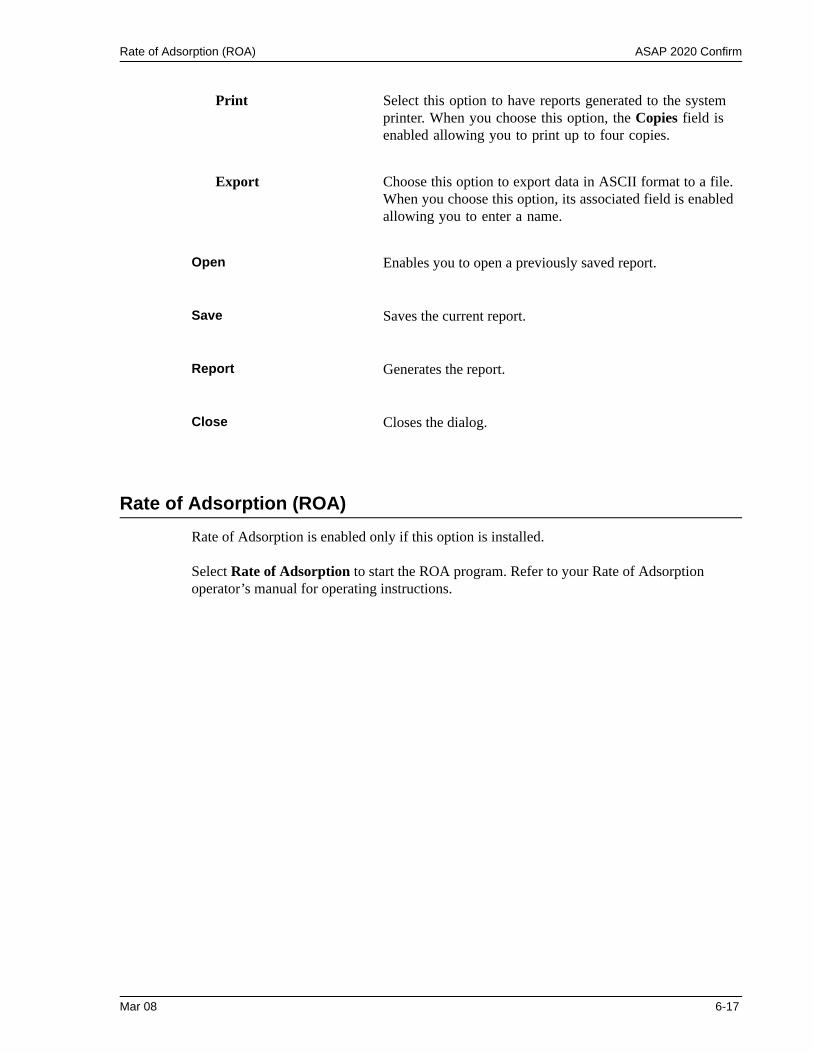
Rate of Adsorption (ROA) ASAP 2020 Confirm
Rate of Adsorption (ROA)Rate of Adsorption is enabled only if this option is installed.
Select Rate of Adsorption to start the ROA program. Refer to your Rate of Adsorption operator’s manual for operating instructions.
Print Select this option to have reports generated to the system printer. When you choose this option, the Copies field is enabled allowing you to print up to four copies.
Export Choose this option to export data in ASCII format to a file. When you choose this option, its associated field is enabled allowing you to enter a name.
Open Enables you to open a previously saved report.
Save Saves the current report.
Report Generates the report.
Close Closes the dialog.
Mar 08 6-17
ASAP 2020 Confirm Printed Reports
Printed Reports
Header
All printed reports (either to the screen or to a printer) contain a header displaying file statistics.
• Tabular and graphical reports contain sample and instrument statistics such as when the file was created and by whom, date and time of analysis, analysis conditions, and so forth.
The headers for these reports also contain notes of any changes to the sample file that occur after analysis.
• Summary report headers contain the same type of information displayed in tabular and graphical reports with the exception of notes.
Onscreen Reports
When you choose Preview as the report destination, reports are printed to the screen. Onscreen reports provide many options for customizing and manipulating reports:
• a tool bar• shortcut menus• zoom feature• axis cross-hairs
When reports are printed to the screen, they are printed in a window like the one shown below. Each requested report is listed in the Reports window on the tool bar; they are also indicated by selectable tabs across the top of the report header. To view a specific report, select its tab or select the report in the Reports window and click Show.
6-18 Mar 08
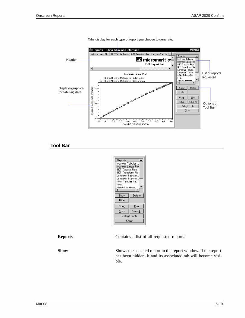
Onscreen Reports ASAP 2020 Confirm
Tool Bar
Displays graphical (or tabular) data
Options on Tool Bar
List of reports requested
Tabs display for each type of report you choose to generate.
Header
Reports Contains a list of all requested reports.
Show Shows the selected report in the report window. If the report has been hidden, it and its associated tab will become visi-ble.
Mar 08 6-19
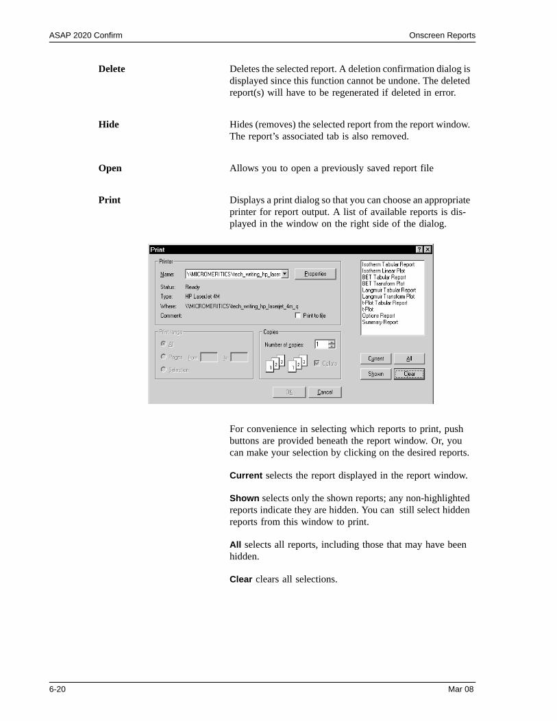
ASAP 2020 Confirm Onscreen Reports
Delete Deletes the selected report. A deletion confirmation dialog is displayed since this function cannot be undone. The deleted report(s) will have to be regenerated if deleted in error.
Hide Hides (removes) the selected report from the report window. The report’s associated tab is also removed.
Open Allows you to open a previously saved report file
Print Displays a print dialog so that you can choose an appropriate printer for report output. A list of available reports is dis-played in the window on the right side of the dialog.
For convenience in selecting which reports to print, push buttons are provided beneath the report window. Or, you can make your selection by clicking on the desired reports.
Current selects the report displayed in the report window.
Shown selects only the shown reports; any non-highlighted reports indicate they are hidden. You can still select hidden reports from this window to print.
All selects all reports, including those that may have been hidden.
Clear clears all selections.
6-20 Mar 08
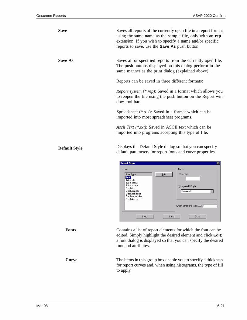
Onscreen Reports ASAP 2020 Confirm
Save Saves all reports of the currently open file in a report format using the same name as the sample file, only with an rep extension. If you wish to specify a name and/or specific reports to save, use the Save As push button.
Save As Saves all or specified reports from the currently open file. The push buttons displayed on this dialog perform in the same manner as the print dialog (explained above).
Reports can be saved in three different formats:
Report system (*.rep): Saved in a format which allows you to reopen the file using the push button on the Report win-dow tool bar.
Spreadsheet (*.xls): Saved in a format which can be imported into most spreadsheet programs.
Ascii Text (*.txt): Saved in ASCII text which can be imported into programs accepting this type of file.
Default Style Displays the Default Style dialog so that you can specify default parameters for report fonts and curve properties.
Fonts Contains a list of report elements for which the font can be edited. Simply highlight the desired element and click Edit; a font dialog is displayed so that you can specify the desired font and attributes.
Curve The items in this group box enable you to specify a thickness for report curves and, when using histograms, the type of fill to apply.
Mar 08 6-21
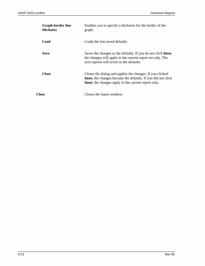
ASAP 2020 Confirm Onscreen Reports
Graph border linethickness
Enables you to specify a thickness for the border of the graph.
Load Loads the last saved defaults.
Save Saves the changes as the defaults. If you do not click Save, the changes will apply to the current report set only. The next reports will revert to the defaults.
Close Closes the dialog and applies the changes. If you clicked Save, the changes become the defaults. If you did not click Save, the changes apply to the current report only.
Close Closes the report window.
6-22 Mar 08
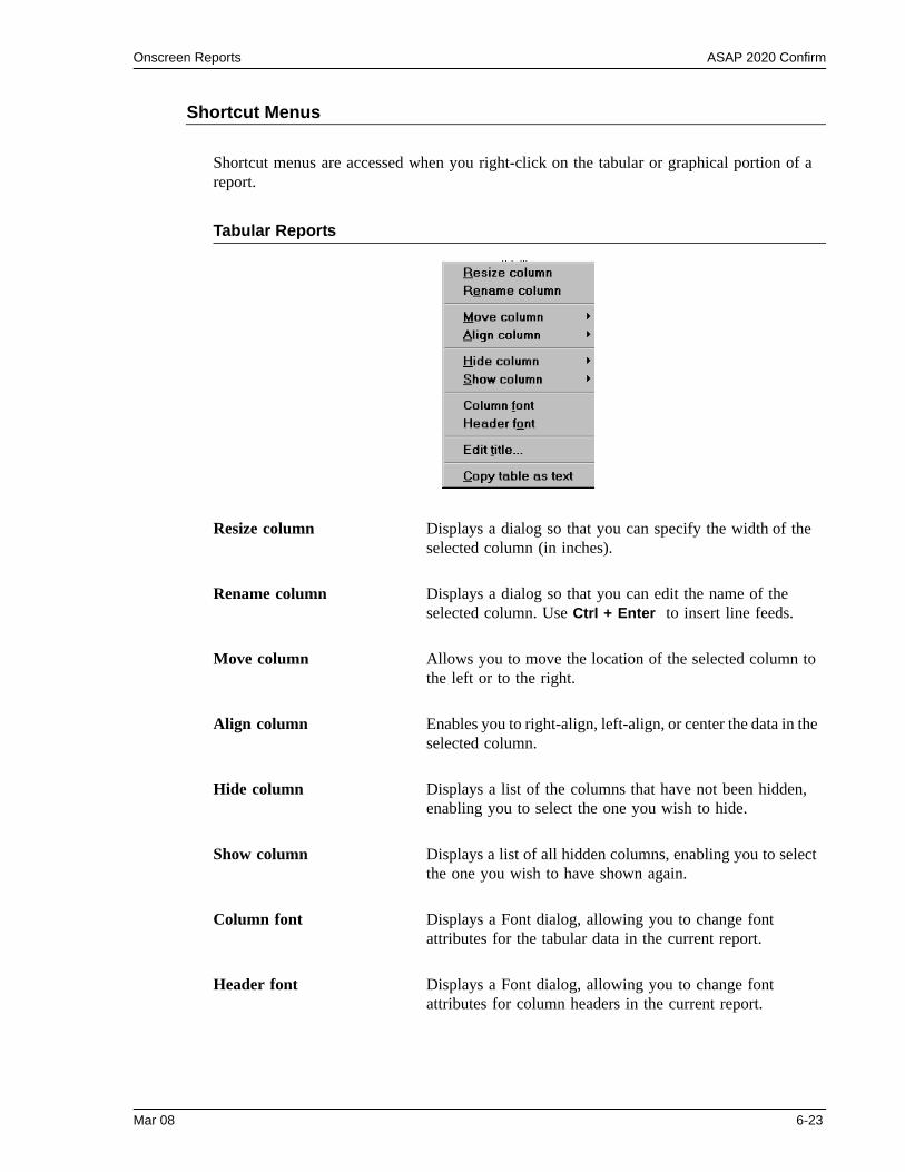
Onscreen Reports ASAP 2020 Confirm
Shortcut Menus
Shortcut menus are accessed when you right-click on the tabular or graphical portion of a report.
Tabular Reports
Resize column Displays a dialog so that you can specify the width of the selected column (in inches).
Rename column Displays a dialog so that you can edit the name of the selected column. Use Ctrl + Enter to insert line feeds.
Move column Allows you to move the location of the selected column to the left or to the right.
Align column Enables you to right-align, left-align, or center the data in the selected column.
Hide column Displays a list of the columns that have not been hidden, enabling you to select the one you wish to hide.
Show column Displays a list of all hidden columns, enabling you to select the one you wish to have shown again.
Column font Displays a Font dialog, allowing you to change font attributes for the tabular data in the current report.
Header font Displays a Font dialog, allowing you to change font attributes for column headers in the current report.
Mar 08 6-23
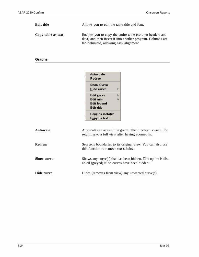
ASAP 2020 Confirm Onscreen Reports
Graphs
Edit title Allows you to edit the table title and font.
Copy table as text Enables you to copy the entire table (column headers and data) and then insert it into another program. Columns are tab-delimited, allowing easy alignment
Autoscale Autoscales all axes of the graph. This function is useful for returning to a full view after having zoomed in.
Redraw Sets axis boundaries to its original view. You can also use this function to remove cross-hairs.
Show curve Shows any curve(s) that has been hidden. This option is dis-abled (greyed) if no curves have been hidden.
Hide curve Hides (removes from view) any unwanted curve(s).
6-24 Mar 08
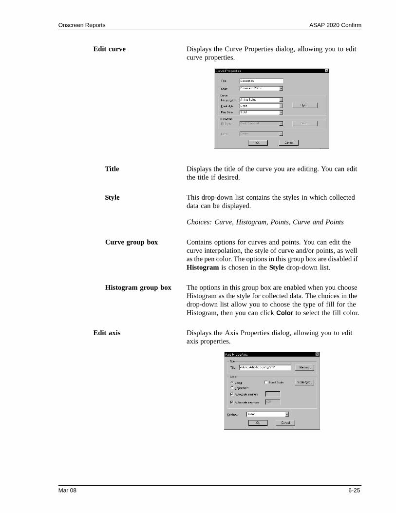
Onscreen Reports ASAP 2020 Confirm
Edit curve Displays the Curve Properties dialog, allowing you to edit curve properties.
Title Displays the title of the curve you are editing. You can edit the title if desired.
Style This drop-down list contains the styles in which collected data can be displayed.
Choices: Curve, Histogram, Points, Curve and Points
Curve group box Contains options for curves and points. You can edit the curve interpolation, the style of curve and/or points, as well as the pen color. The options in this group box are disabled if Histogram is chosen in the Style drop-down list.
Histogram group box The options in this group box are enabled when you choose Histogram as the style for collected data. The choices in the drop-down list allow you to choose the type of fill for the Histogram, then you can click Color to select the fill color.
Edit axis Displays the Axis Properties dialog, allowing you to edit axis properties.
Mar 08 6-25
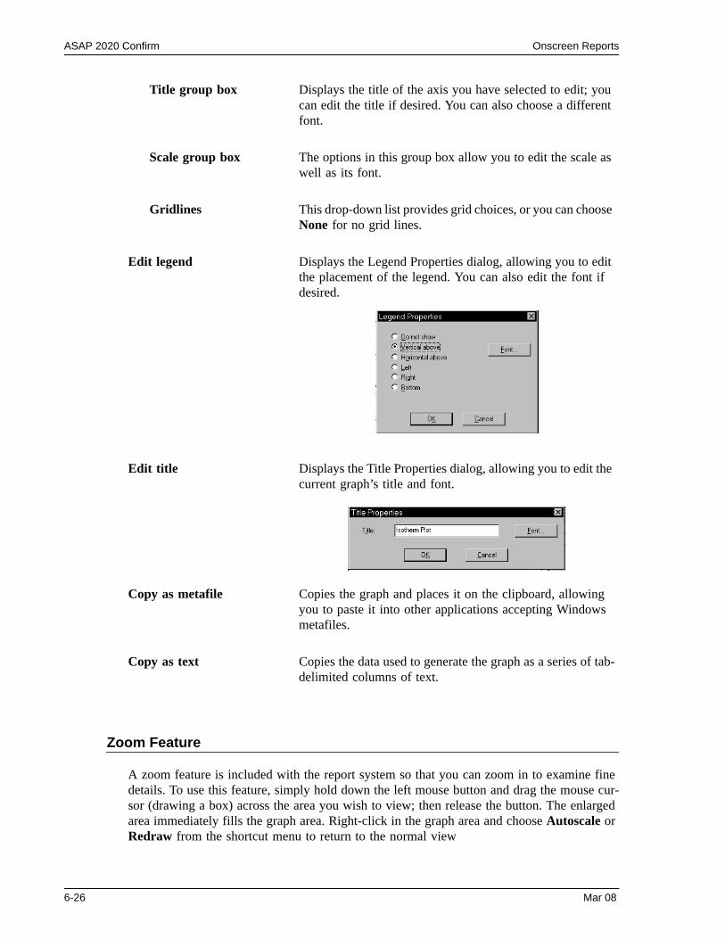
ASAP 2020 Confirm Onscreen Reports
Zoom Feature
A zoom feature is included with the report system so that you can zoom in to examine fine details. To use this feature, simply hold down the left mouse button and drag the mouse cur-sor (drawing a box) across the area you wish to view; then release the button. The enlarged area immediately fills the graph area. Right-click in the graph area and choose Autoscale or Redraw from the shortcut menu to return to the normal view
Title group box Displays the title of the axis you have selected to edit; you can edit the title if desired. You can also choose a different font.
Scale group box The options in this group box allow you to edit the scale as well as its font.
Gridlines This drop-down list provides grid choices, or you can choose None for no grid lines.
Edit legend Displays the Legend Properties dialog, allowing you to edit the placement of the legend. You can also edit the font if desired.
Edit title Displays the Title Properties dialog, allowing you to edit the current graph’s title and font.
Copy as metafile Copies the graph and places it on the clipboard, allowing you to paste it into other applications accepting Windows metafiles.
Copy as text Copies the data used to generate the graph as a series of tab-delimited columns of text.
6-26 Mar 08
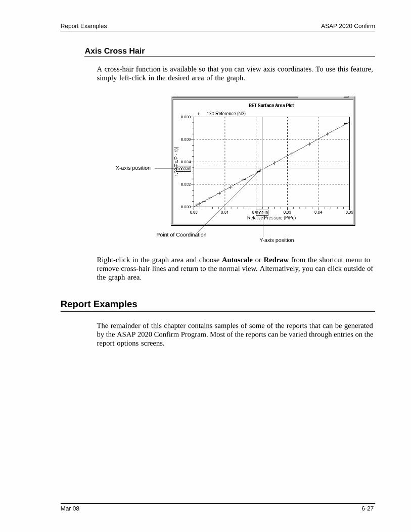
Report Examples ASAP 2020 Confirm
Axis Cross Hair
A cross-hair function is available so that you can view axis coordinates. To use this feature, simply left-click in the desired area of the graph.
Right-click in the graph area and choose Autoscale or Redraw from the shortcut menu to remove cross-hair lines and return to the normal view. Alternatively, you can click outside of the graph area.
Report Examples
The remainder of this chapter contains samples of some of the reports that can be generated by the ASAP 2020 Confirm Program. Most of the reports can be varied through entries on the report options screens.
Point of CoordinationY-axis position
X-axis position
Mar 08 6-27
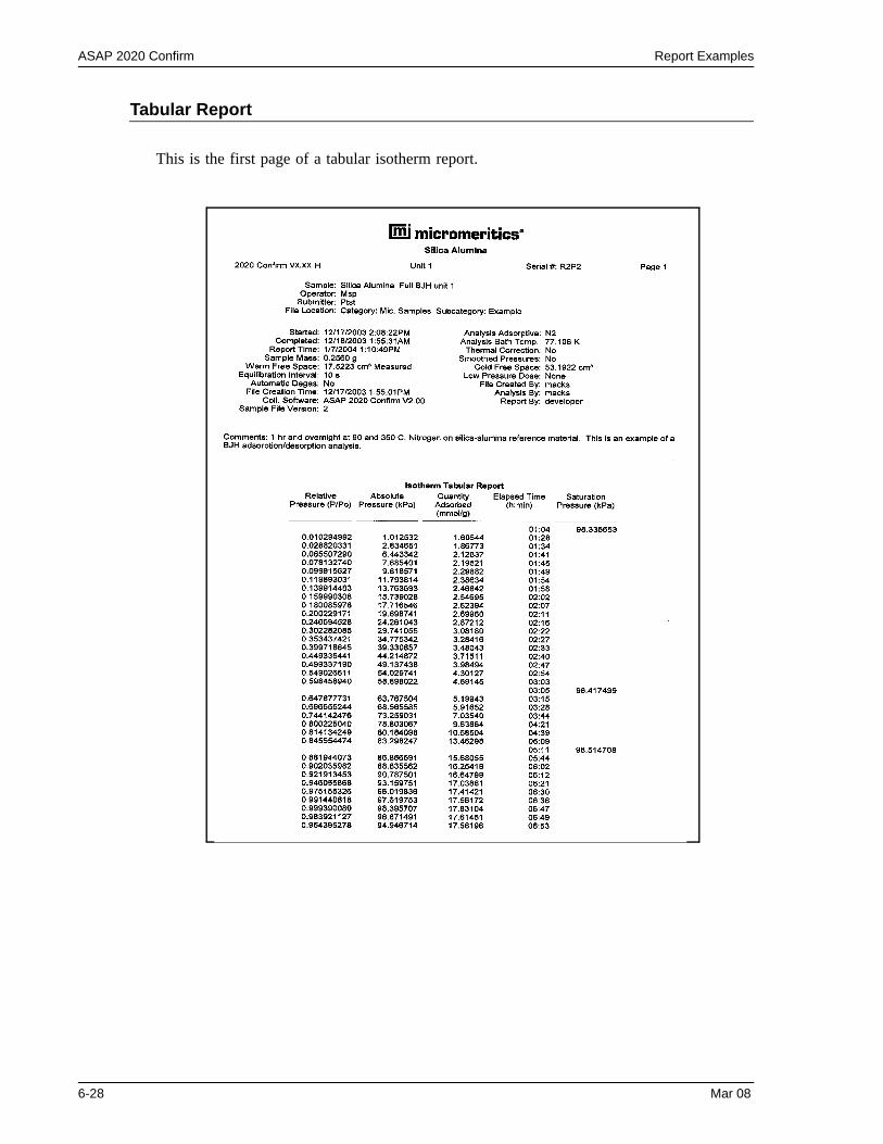
ASAP 2020 Confirm Report Examples
Tabular Report
This is the first page of a tabular isotherm report.
6-28 Mar 08
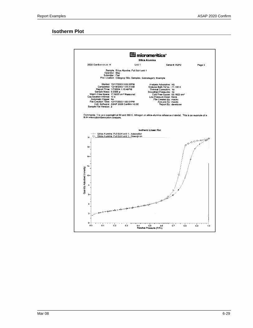
Report Examples ASAP 2020 Confirm
Isotherm Plot
Mar 08 6-29
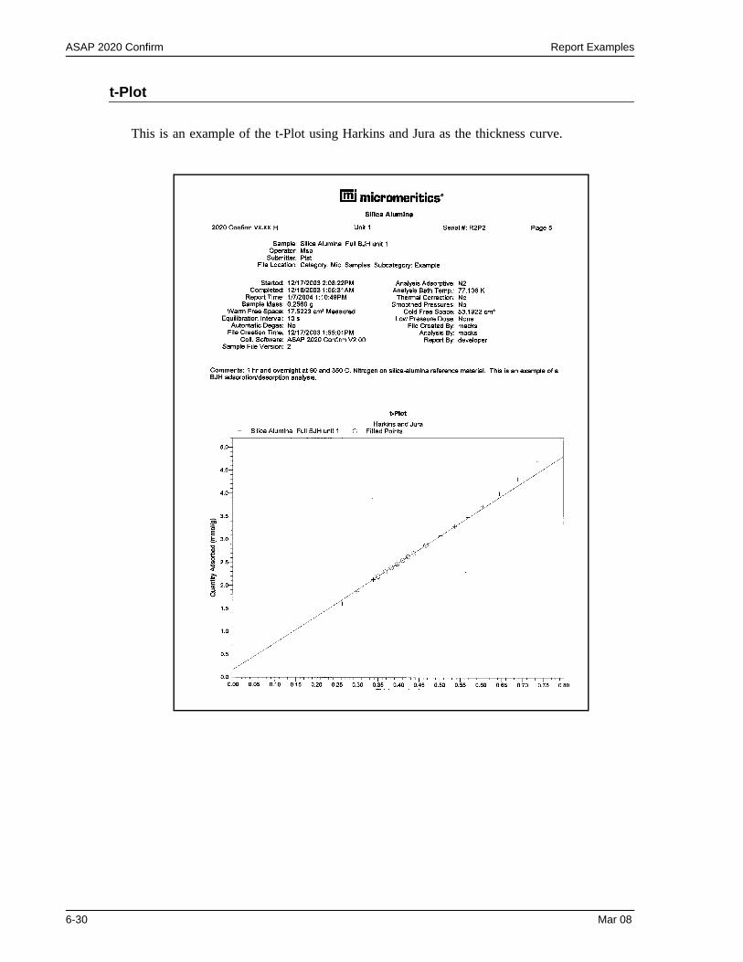
ASAP 2020 Confirm Report Examples
t-Plot
This is an example of the t-Plot using Harkins and Jura as the thickness curve.
6-30 Mar 08
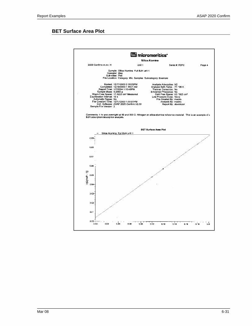
Report Examples ASAP 2020 Confirm
BET Surface Area Plot
Mar 08 6-31
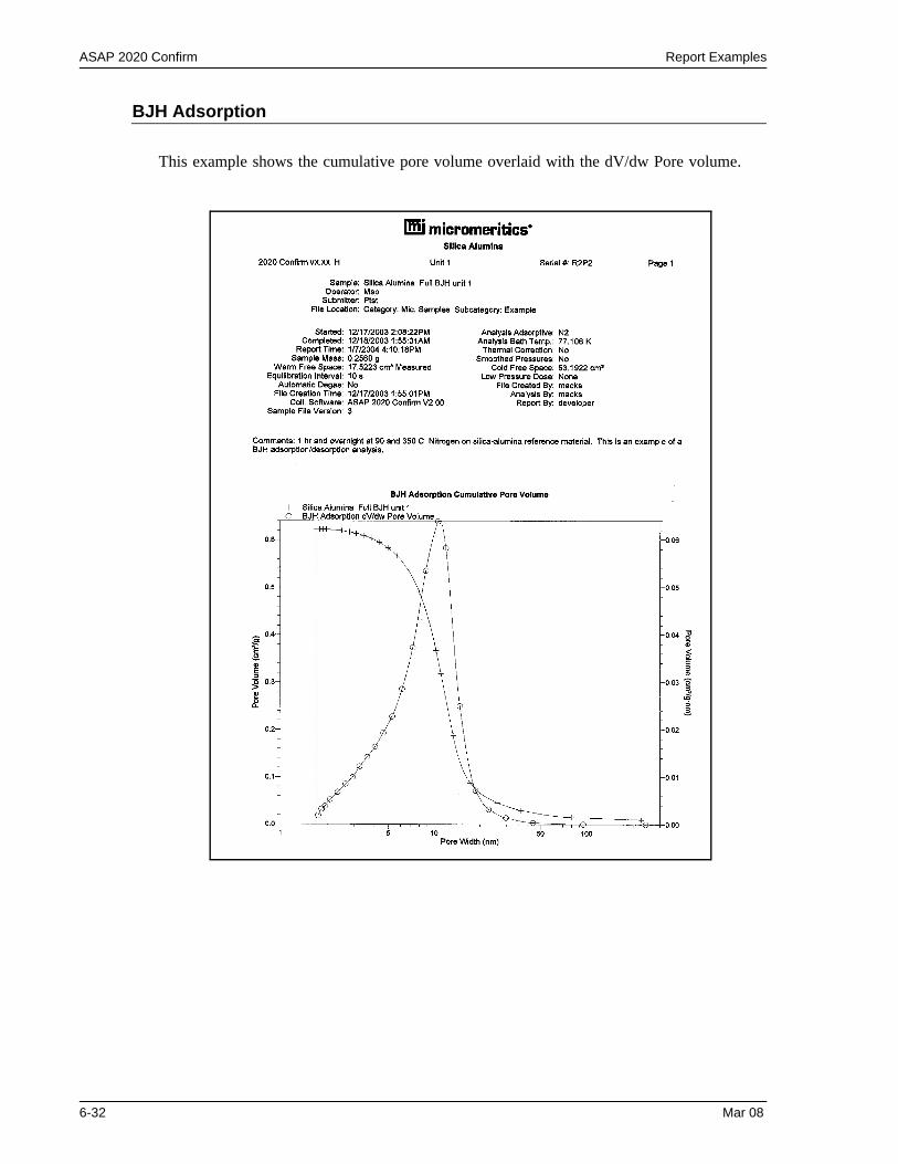
ASAP 2020 Confirm Report Examples
BJH Adsorption
This example shows the cumulative pore volume overlaid with the dV/dw Pore volume.
6-32 Mar 08
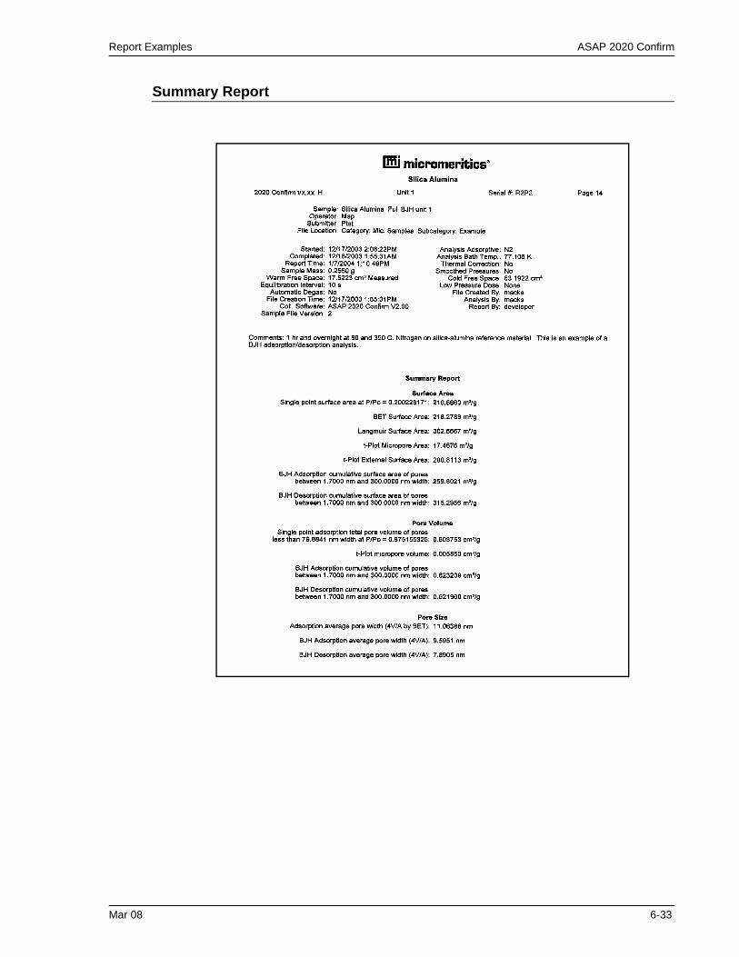
Report Examples ASAP 2020 Confirm
Summary Report
Mar 08 6-33
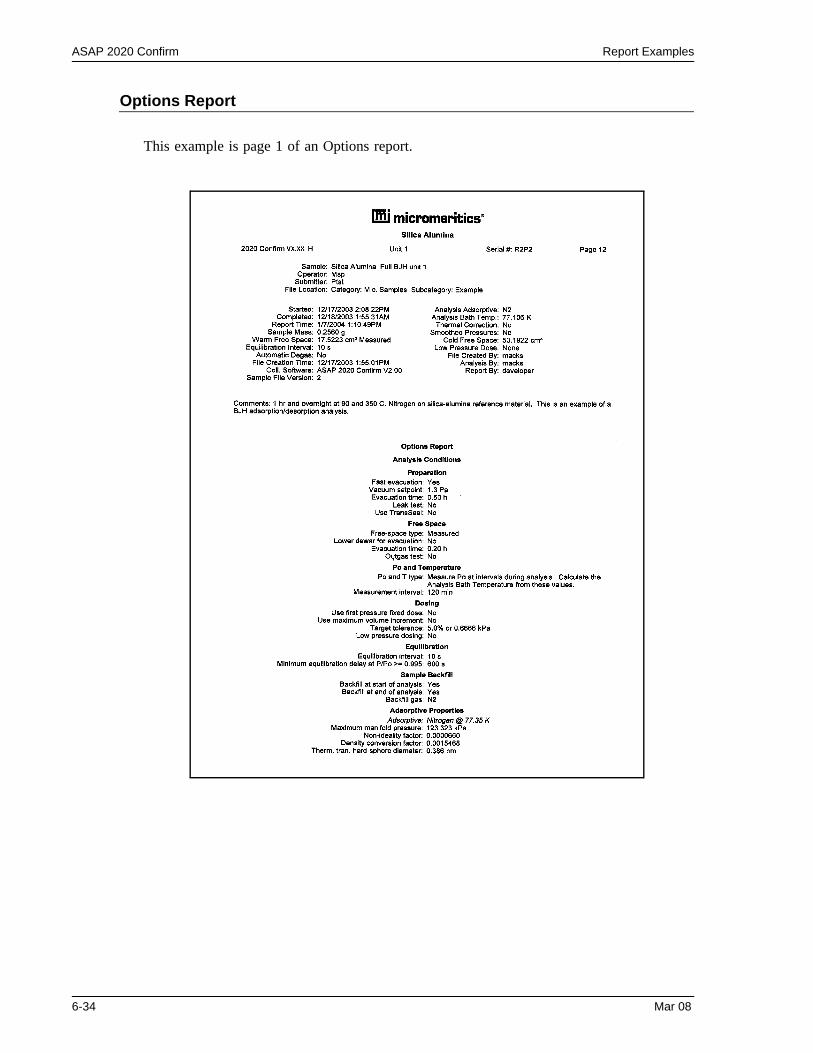
ASAP 2020 Confirm Report Examples
Options Report
This example is page 1 of an Options report.
6-34 Mar 08
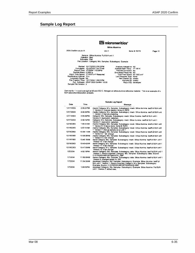
Report Examples ASAP 2020 Confirm
Sample Log Report
Mar 08 6-35

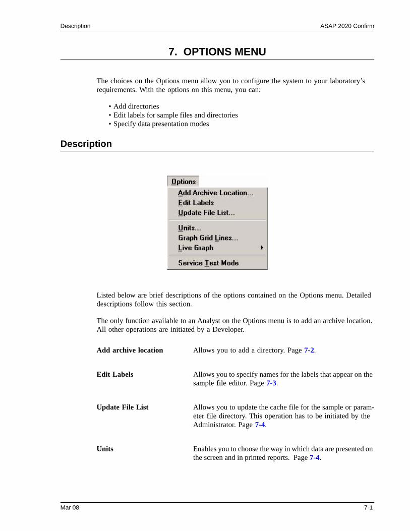
Description ASAP 2020 Confirm
7. OPTIONS MENU
The choices on the Options menu allow you to configure the system to your laboratory’s requirements. With the options on this menu, you can:
• Add directories• Edit labels for sample files and directories• Specify data presentation modes
Description
Listed below are brief descriptions of the options contained on the Options menu. Detailed descriptions follow this section.
The only function available to an Analyst on the Options menu is to add an archive location. All other operations are initiated by a Developer.
Add archive location Allows you to add a directory. Page 7-2.
Edit Labels Allows you to specify names for the labels that appear on the sample file editor. Page 7-3.
Update File List Allows you to update the cache file for the sample or param-eter file directory. This operation has to be initiated by the Administrator. Page 7-4.
Units Enables you to choose the way in which data are presented on the screen and in printed reports. Page 7-4.
Mar 08 7-1
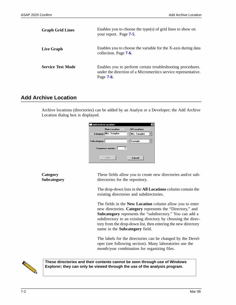
ASAP 2020 Confirm Add Archive Location
Add Archive Location
Archive locations (directories) can be added by an Analyst or a Developer; the Add Archive Location dialog box is displayed.
Graph Grid Lines Enables you to choose the type(s) of grid lines to show on your report. Page 7-5.
Live Graph Enables you to choose the variable for the X-axis during data colleciton. Page 7-6.
Service Test Mode Enables you to perform certain troubleshooting procedures. under the direction of a Micromeritics service representative. Page 7-6.
CategorySubcategory
These fields allow you to create new directories and/or sub-directories for the repository.
The drop-down lists in the All Locations column contain the existing directories and subdirectories.
The fields in the New Location column allow you to enter new directories. Category represents the “Directory,” and Subcategory represents the “subdirectory.” You can add a subdirectory to an existing directory by choosing the direc-tory from the drop-down list, then entering the new directory name in the Subcategory field.
The labels for the directories can be changed by the Devel-oper (see following section). Many laboratories use the month/year combination for organizing files.
These directories and their contents cannot be seen through use of Windows Explorer; they can only be viewed through the use of the analysis program.
7-2 Mar 08
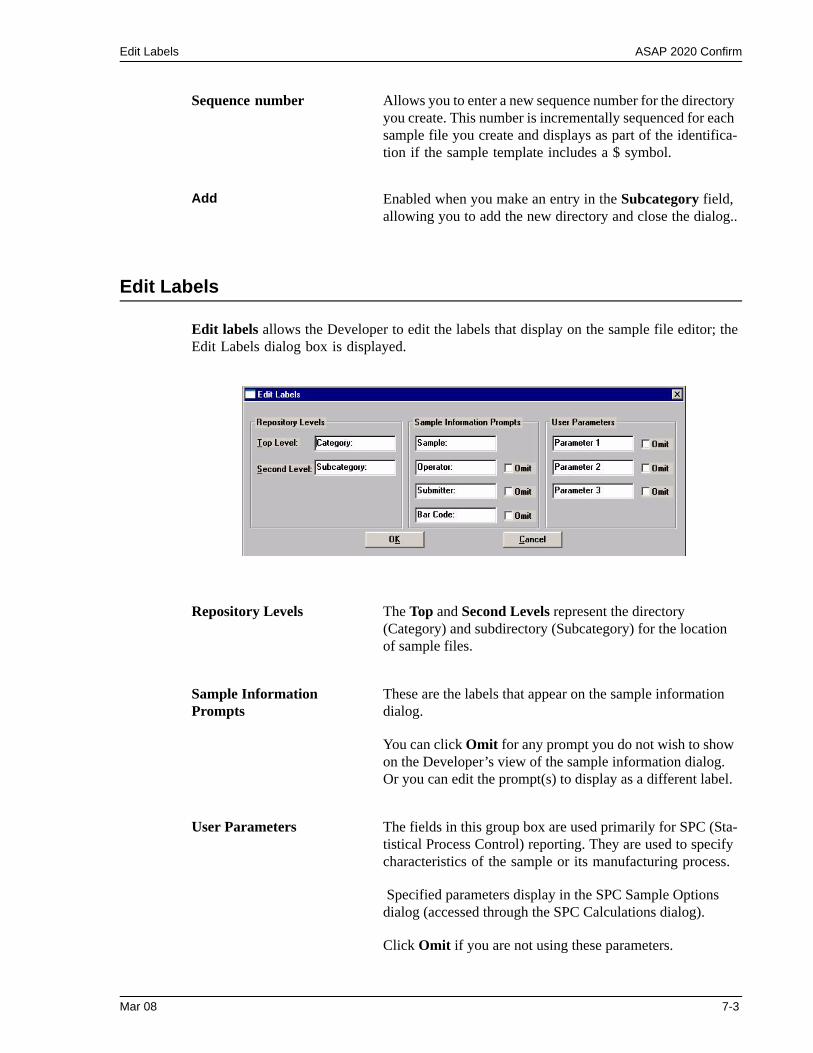
Edit Labels ASAP 2020 Confirm
Edit Labels
Edit labels allows the Developer to edit the labels that display on the sample file editor; the Edit Labels dialog box is displayed.
Sequence number Allows you to enter a new sequence number for the directory you create. This number is incrementally sequenced for each sample file you create and displays as part of the identifica-tion if the sample template includes a $ symbol.
Add Enabled when you make an entry in the Subcategory field, allowing you to add the new directory and close the dialog..
Repository Levels The Top and Second Levels represent the directory (Category) and subdirectory (Subcategory) for the location of sample files.
Sample Information Prompts
These are the labels that appear on the sample information dialog.
You can click Omit for any prompt you do not wish to show on the Developer’s view of the sample information dialog. Or you can edit the prompt(s) to display as a different label.
User Parameters The fields in this group box are used primarily for SPC (Sta-tistical Process Control) reporting. They are used to specify characteristics of the sample or its manufacturing process.
Specified parameters display in the SPC Sample Options dialog (accessed through the SPC Calculations dialog).
Click Omit if you are not using these parameters.
Mar 08 7-3
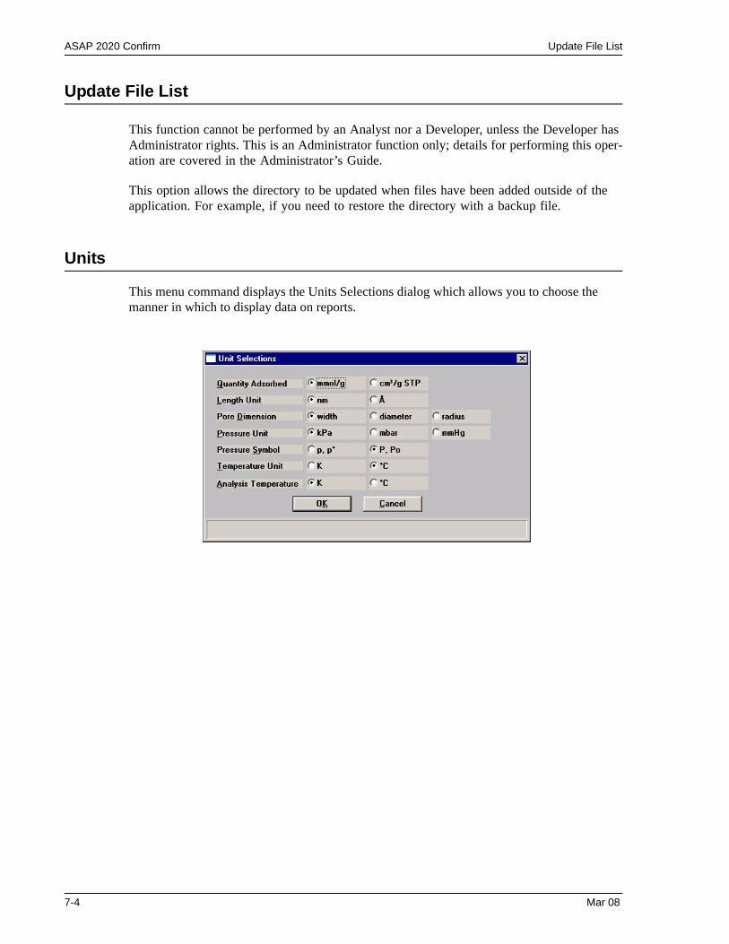
ASAP 2020 Confirm Update File List
Update File List
This function cannot be performed by an Analyst nor a Developer, unless the Developer has Administrator rights. This is an Administrator function only; details for performing this oper-ation are covered in the Administrator’s Guide.
This option allows the directory to be updated when files have been added outside of the application. For example, if you need to restore the directory with a backup file.
Units
This menu command displays the Units Selections dialog which allows you to choose the manner in which to display data on reports.
7-4 Mar 08
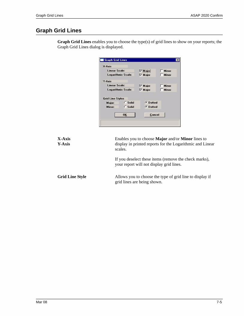
Graph Grid Lines ASAP 2020 Confirm
Graph Grid Lines
Graph Grid Lines enables you to choose the type(s) of grid lines to show on your reports; the Graph Grid Lines dialog is displayed.
X-AxisY-Axis
Enables you to choose Major and/or Minor lines to display in printed reports for the Logarithmic and Linear scales.
If you deselect these items (remove the check marks), your report will not display grid lines.
Grid Line Style Allows you to choose the type of grid line to display if grid lines are being shown.
Mar 08 7-5
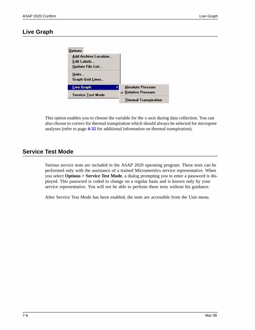
ASAP 2020 Confirm Live Graph
Live Graph
This option enables you to choose the variable for the x-axis during data collection. You can also choose to correct for thermal transpiration which should always be selected for micropore analyses (refer to page 4-32 for additional information on thermal transpiration).
Service Test Mode
Various service tests are included in the ASAP 2020 operating program. These tests can be performed only with the assistance of a trained Micromeritics service representative. When you select Options > Service Test Mode, a dialog prompting you to enter a password is dis-played. This password is coded to change on a regular basis and is known only by your service representative. You will not be able to perform these tests without his guidance.
After Service Test Mode has been enabled, the tests are accessible from the Unit menu.
7-6 Mar 08
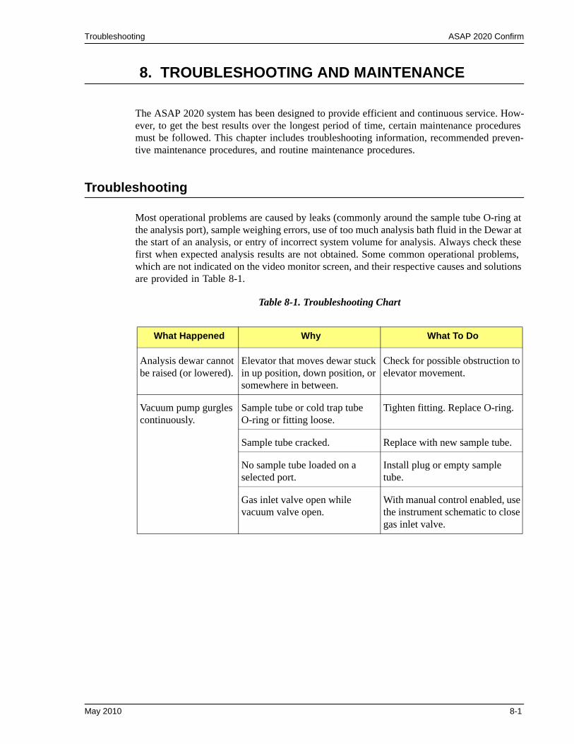
Troubleshooting ASAP 2020 Confirm
8. TROUBLESHOOTING AND MAINTENANCE
The ASAP 2020 system has been designed to provide efficient and continuous service. How-ever, to get the best results over the longest period of time, certain maintenance procedures must be followed. This chapter includes troubleshooting information, recommended preven-tive maintenance procedures, and routine maintenance procedures.
Troubleshooting
Most operational problems are caused by leaks (commonly around the sample tube O-ring at the analysis port), sample weighing errors, use of too much analysis bath fluid in the Dewar at the start of an analysis, or entry of incorrect system volume for analysis. Always check these first when expected analysis results are not obtained. Some common operational problems, which are not indicated on the video monitor screen, and their respective causes and solutions are provided in Table 8-1.
Table 8-1. Troubleshooting Chart
What Happened Why What To Do
Analysis dewar cannot be raised (or lowered).
Elevator that moves dewar stuck in up position, down position, or somewhere in between.
Check for possible obstruction to elevator movement.
Vacuum pump gurgles continuously.
Sample tube or cold trap tube O-ring or fitting loose.
Tighten fitting. Replace O-ring.
Sample tube cracked. Replace with new sample tube.
No sample tube loaded on a selected port.
Install plug or empty sample tube.
Gas inlet valve open while vacuum valve open.
With manual control enabled, use the instrument schematic to close gas inlet valve.
May 2010 8-1
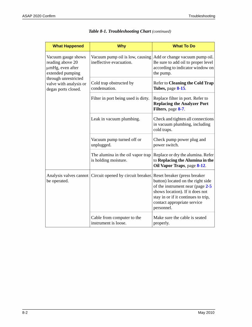
ASAP 2020 Confirm Troubleshooting
Table 8-1. Troubleshooting Chart (continued)
What Happened Why What To Do
Vacuum gauge shows reading above 20 µmHg, even after extended pumping through unrestricted valve with analysis or degas ports closed.
Vacuum pump oil is low, causing ineffective evacuation.
Add or change vacuum pump oil. Be sure to add oil to proper level according to indicator window on the pump.
Cold trap obstructed by condensation.
Refer to Cleaning the Cold Trap Tubes, page 8-15.
Filter in port being used is dirty. Replace filter in port. Refer to Replacing the Analyzer Port Filters, page 8-7.
Leak in vacuum plumbing. Check and tighten all connections in vacuum plumbing, including cold traps.
Vacuum pump turned off or unplugged.
Check pump power plug and power switch.
The alumina in the oil vapor trap is holding moisture.
Replace or dry the alumina. Refer to Replacing the Alumina in the Oil Vapor Traps, page 8-12.
Analysis valves cannot be operated.
Circuit opened by circuit breaker. Reset breaker (press breaker button) located on the right side of the instrument near (page 2-5 shows location). If it does not stay in or if it continues to trip, contact appropriate service personnel.
Cable from computer to the instrument is loose.
Make sure the cable is seated properly.
8-2 May 2010
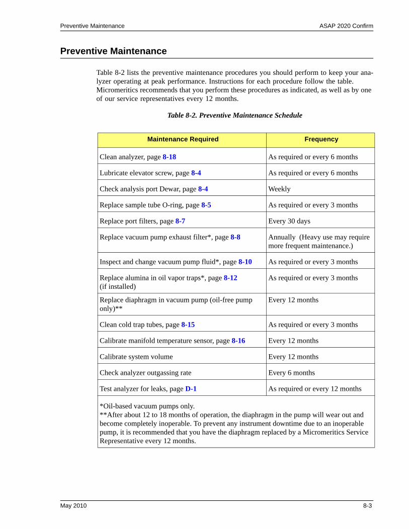
Preventive Maintenance ASAP 2020 Confirm
Preventive Maintenance
Table 8-2 lists the preventive maintenance procedures you should perform to keep your ana-lyzer operating at peak performance. Instructions for each procedure follow the table. Micromeritics recommends that you perform these procedures as indicated, as well as by one of our service representatives every 12 months.
Table 8-2. Preventive Maintenance Schedule
Maintenance Required Frequency
Clean analyzer, page 8-18 As required or every 6 months
Lubricate elevator screw, page 8-4 As required or every 6 months
Check analysis port Dewar, page 8-4 Weekly
Replace sample tube O-ring, page 8-5 As required or every 3 months
Replace port filters, page 8-7 Every 30 days
Replace vacuum pump exhaust filter*, page 8-8 Annually (Heavy use may require more frequent maintenance.)
Inspect and change vacuum pump fluid*, page 8-10 As required or every 3 months
Replace alumina in oil vapor traps*, page 8-12 (if installed)
As required or every 3 months
Replace diaphragm in vacuum pump (oil-free pump only)**
Every 12 months
Clean cold trap tubes, page 8-15 As required or every 3 months
Calibrate manifold temperature sensor, page 8-16 Every 12 months
Calibrate system volume Every 12 months
Check analyzer outgassing rate Every 6 months
Test analyzer for leaks, page D-1 As required or every 12 months
*Oil-based vacuum pumps only.**After about 12 to 18 months of operation, the diaphragm in the pump will wear out and become completely inoperable. To prevent any instrument downtime due to an inoperable pump, it is recommended that you have the diaphragm replaced by a Micromeritics Service Representative every 12 months.
May 2010 8-3
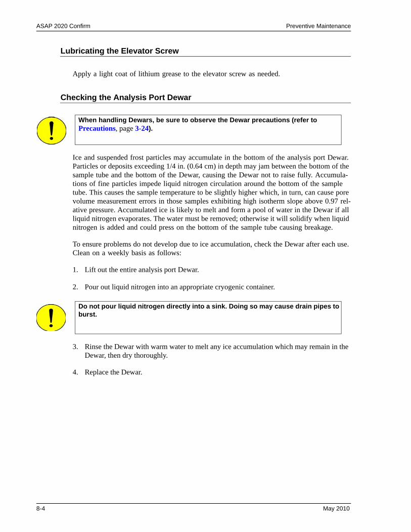
ASAP 2020 Confirm Preventive Maintenance
Lubricating the Elevator Screw
Apply a light coat of lithium grease to the elevator screw as needed.
Checking the Analysis Port Dewar
Ice and suspended frost particles may accumulate in the bottom of the analysis port Dewar. Particles or deposits exceeding 1/4 in. (0.64 cm) in depth may jam between the bottom of the sample tube and the bottom of the Dewar, causing the Dewar not to raise fully. Accumula-tions of fine particles impede liquid nitrogen circulation around the bottom of the sample tube. This causes the sample temperature to be slightly higher which, in turn, can cause pore volume measurement errors in those samples exhibiting high isotherm slope above 0.97 rel-ative pressure. Accumulated ice is likely to melt and form a pool of water in the Dewar if all liquid nitrogen evaporates. The water must be removed; otherwise it will solidify when liquid nitrogen is added and could press on the bottom of the sample tube causing breakage.
To ensure problems do not develop due to ice accumulation, check the Dewar after each use. Clean on a weekly basis as follows:
1. Lift out the entire analysis port Dewar.
2. Pour out liquid nitrogen into an appropriate cryogenic container.
3. Rinse the Dewar with warm water to melt any ice accumulation which may remain in the Dewar, then dry thoroughly.
4. Replace the Dewar.
When handling Dewars, be sure to observe the Dewar precautions (refer to Precautions, page 3-24).
Do not pour liquid nitrogen directly into a sink. Doing so may cause drain pipes to burst.
8-4 May 2010
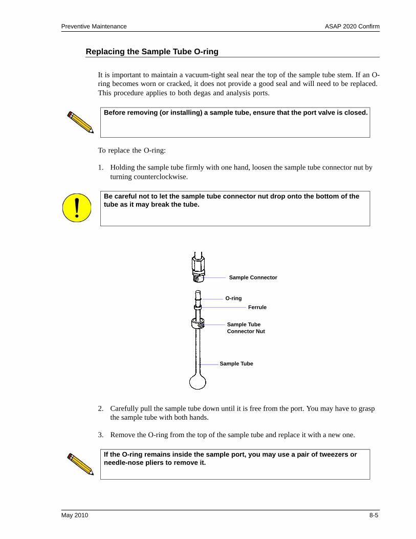
Preventive Maintenance ASAP 2020 Confirm
Replacing the Sample Tube O-ring
It is important to maintain a vacuum-tight seal near the top of the sample tube stem. If an O-ring becomes worn or cracked, it does not provide a good seal and will need to be replaced. This procedure applies to both degas and analysis ports.
To replace the O-ring:
1. Holding the sample tube firmly with one hand, loosen the sample tube connector nut by turning counterclockwise.
2. Carefully pull the sample tube down until it is free from the port. You may have to grasp the sample tube with both hands.
3. Remove the O-ring from the top of the sample tube and replace it with a new one.
Before removing (or installing) a sample tube, ensure that the port valve is closed.
Be careful not to let the sample tube connector nut drop onto the bottom of the tube as it may break the tube.
Sample Connector
O-ringFerrule
Sample Tube Connector Nut
Sample Tube
If the O-ring remains inside the sample port, you may use a pair of tweezers or needle-nose pliers to remove it.
May 2010 8-5

ASAP 2020 Confirm Preventive Maintenance
4. After the new O-ring is in place, insert the sample tube back into the sample port until it is fully seated.
5. Slide the sample tube connector nut up the tube (the ferrule and O-ring will move along with the connector nut). Then, turning clockwise, hand-tighten the connector nut to the sample connector.
8-6 May 2010
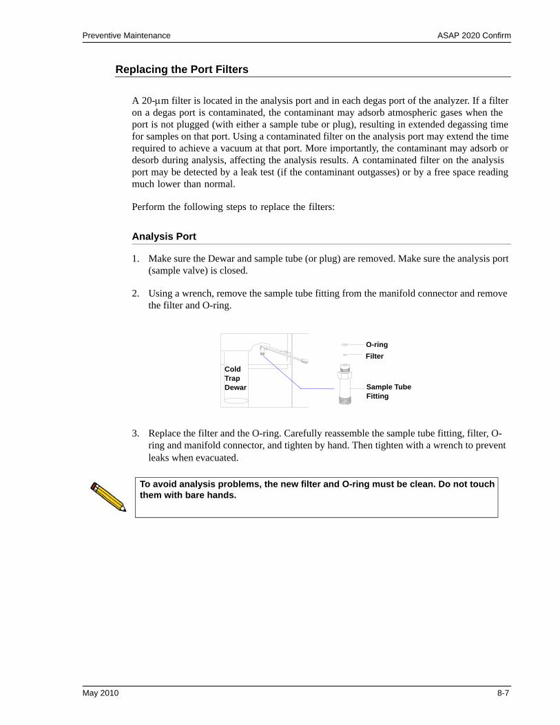
Preventive Maintenance ASAP 2020 Confirm
Replacing the Port Filters
A 20-µm filter is located in the analysis port and in each degas port of the analyzer. If a filter on a degas port is contaminated, the contaminant may adsorb atmospheric gases when the port is not plugged (with either a sample tube or plug), resulting in extended degassing time for samples on that port. Using a contaminated filter on the analysis port may extend the time required to achieve a vacuum at that port. More importantly, the contaminant may adsorb or desorb during analysis, affecting the analysis results. A contaminated filter on the analysis port may be detected by a leak test (if the contaminant outgasses) or by a free space reading much lower than normal.
Perform the following steps to replace the filters:
Analysis Port
1. Make sure the Dewar and sample tube (or plug) are removed. Make sure the analysis port (sample valve) is closed.
2. Using a wrench, remove the sample tube fitting from the manifold connector and remove the filter and O-ring.
3. Replace the filter and the O-ring. Carefully reassemble the sample tube fitting, filter, O-ring and manifold connector, and tighten by hand. Then tighten with a wrench to prevent leaks when evacuated.
O-ringFilter
Sample Tube Fitting
Cold Trap Dewar
To avoid analysis problems, the new filter and O-ring must be clean. Do not touch them with bare hands.
May 2010 8-7
ASAP 2020 Confirm Preventive Maintenance
Degas Port
1. Using a wrench, remove the degas port fitting and remove the filter and O-ring.
2. Replace the filter and the O-ring. Carefully reassemble the sample tube fitting, filter, O-ring and manifold connector, and tighten by hand. Then tighten with the wrenches to prevent leaks when evacuated.
Replacing the Vacuum Pump Exhaust Filter
The gases used by the ASAP 2020 are exhausted by vacuum pumps. An exhaust filter is installed on the exhaust port of each vacuum pump. The filter minimizes the release of oil vapor and should be replaced when it becomes so saturated with oil that it is ineffective.
1. Using a flat-head screwdriver, remove the screws from the vacuum pump panel on the front of the analyzer, then remove the panel to access the pump.
To avoid degassing problems, the new filter and O-ring must be clean. Do not tough them with bare hands.
This procedure does not apply, and is not required, for dry vacuum pumps.
Exhaust filters are used on the vacuum pump to minimize the release of oil vapors. The gases used are diluted substantially upon being released form the vacuum pumps. However, it may be desirable in some locations to provide a fume hood for added protection from hazardous gases and vapors released into the work area.
8-8 May 2010
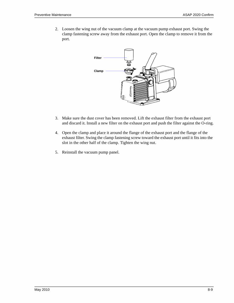
Preventive Maintenance ASAP 2020 Confirm
2. Loosen the wing nut of the vacuum clamp at the vacuum pump exhaust port. Swing the clamp fastening screw away from the exhaust port. Open the clamp to remove it from the port.
3. Make sure the dust cover has been removed. Lift the exhaust filter from the exhaust port and discard it. Install a new filter on the exhaust port and push the filter against the O-ring.
4. Open the clamp and place it around the flange of the exhaust port and the flange of the exhaust filter. Swing the clamp fastening screw toward the exhaust port until it fits into the slot in the other half of the clamp. Tighten the wing nut.
5. Reinstall the vacuum pump panel.
Filter
Clamp
May 2010 8-9
ASAP 2020 Confirm Preventive Maintenance
Inspecting and Changing Vacuum Pump Fluid
The fluid in the vacuum pump should be changed every three months or when the efficiency of the vacuum pump declines (requiring increased time to reach vacuum levels). The fluid can first be inspected to determine if a change is necessary.
Use oil supplied by Micromeritics, or refer to the manual for the vacuum pump for other acceptable oils.
Inspecting Fluid
Inspect the fluid as follows:
1. Remove the vacuum pump panel (located on the left front side of the analyzer).
2. View the vacuum pump fluid through the oil level indicator window. Fluid in good condition is clean, clear or light in color, and transparent. If the color of the fluid is darkened, the fluid should be changed.
Changing Fluid
Change the fluid as follows:
1. Place the analyzer ON/OFF switch in the OFF position.
2. Remove the vacuum pump panel (if not already removed)
3. Disconnect the vacuum pump power cord from its power source..
4. Disconnect the vacuum pump hose from the top of the vacuum pump.
5. Grasp the handle on top of the vacuum pump and lift it out of the analyzer; place the vacuum pump on a work table.
This procedure does not apply, and is not required, for dry vacuum pumps.
If the high vacuum pump is installed, wait for it to completely stop (approximately 10 minutes).
Always drain the vacuum pump while the pump is warm and switched off (unplugged).
8-10 May 2010
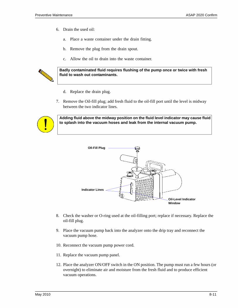
Preventive Maintenance ASAP 2020 Confirm
6. Drain the used oil:
a. Place a waste container under the drain fitting.
b. Remove the plug from the drain spout.
c. Allow the oil to drain into the waste container.
d. Replace the drain plug.
7. Remove the Oil-fill plug; add fresh fluid to the oil-fill port until the level is midway between the two indicator lines.
8. Check the washer or O-ring used at the oil-filling port; replace if necessary. Replace the oil-fill plug.
9. Place the vacuum pump back into the analyzer onto the drip tray and reconnect the vacuum pump hose.
10. Reconnect the vacuum pump power cord.
11. Replace the vacuum pump panel.
12. Place the analyzer ON/OFF switch in the ON position. The pump must run a few hours (or overnight) to eliminate air and moisture from the fresh fluid and to produce efficient vacuum operations.
Badly contaminated fluid requires flushing of the pump once or twice with fresh fluid to wash out contaminants.
Adding fluid above the midway position on the fluid level indicator may cause fluid to splash into the vacuum hoses and leak from the internal vacuum pump.
OIl-Fill Plug
Indicator Lines
Oil-Level Indicator Window
May 2010 8-11
ASAP 2020 Confirm Preventive Maintenance
Replacing the Alumina in the Oil Vapor Traps
The activated alumina in the oil vapor traps becomes saturated during use. The alumina should be replaced if any of the following conditions exist:
• The alumina has been used for a three-month period.• Oil has accumulated in the cold trap.• Most of the alumina pellets are no longer white.
Perform the following steps to replace the alumina:
1. Place the analyzer ON/OFF switch in the OFF position., and turn off the vacuum pump.
2. Remove the vacuum pump panel.
3. Prepare fresh alumina as follows:
a. Heat an oven between 250 °C and 350 °C.
b. Pour about 180 grams of alumina into a glass or metal container for each trap (approximately 250 mL if a graduated beaker is used). Place the container in the oven.
c. Bake the alumina for two hours; turn off the oven.
d. Allow the alumina to cool in the oven before pouring it into the traps.
When you replace the alumina, you may also need to change the vacuum pump oil if the interval between changes of alumina has been short.
Do not perform the following procedure on used alumina. The resultant oil vapors may cause a fire or an explosion.
If the high vacuum pump is installed, wait for it to completely stop (approximately 10 minutes).
8-12 May 2010
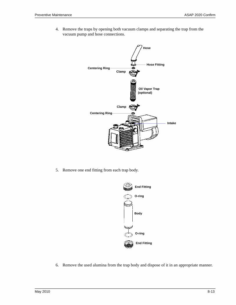
Preventive Maintenance ASAP 2020 Confirm
4. Remove the traps by opening both vacuum clamps and separating the trap from the vacuum pump and hose connections.
5. Remove one end fitting from each trap body.
6. Remove the used alumina from the trap body and dispose of it in an appropriate manner.
Hose Fitting
Hose
Oil Vapor Trap (optional)
Clamp
Clamp
Centering Ring
Intake
Centering Ring
End Fitting
End Fitting
Body
O-ring
O-ring
May 2010 8-13
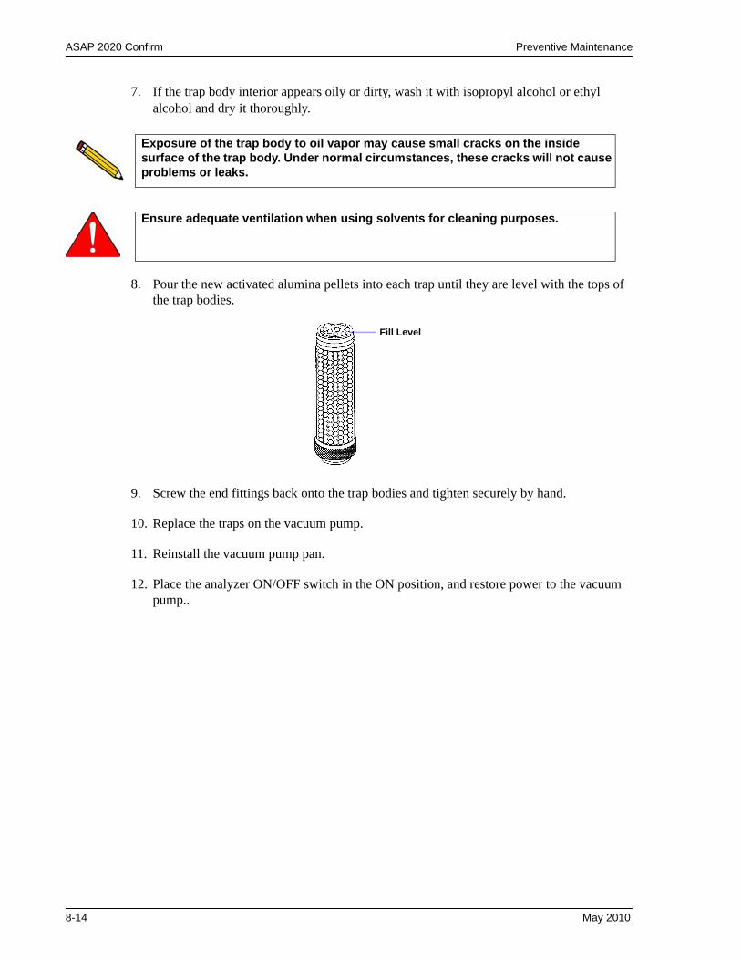
ASAP 2020 Confirm Preventive Maintenance
7. If the trap body interior appears oily or dirty, wash it with isopropyl alcohol or ethyl alcohol and dry it thoroughly.
8. Pour the new activated alumina pellets into each trap until they are level with the tops of the trap bodies.
9. Screw the end fittings back onto the trap bodies and tighten securely by hand.
10. Replace the traps on the vacuum pump.
11. Reinstall the vacuum pump pan.
12. Place the analyzer ON/OFF switch in the ON position, and restore power to the vacuum pump..
Exposure of the trap body to oil vapor may cause small cracks on the inside surface of the trap body. Under normal circumstances, these cracks will not cause problems or leaks.
Ensure adequate ventilation when using solvents for cleaning purposes.
Fill Level
8-14 May 2010
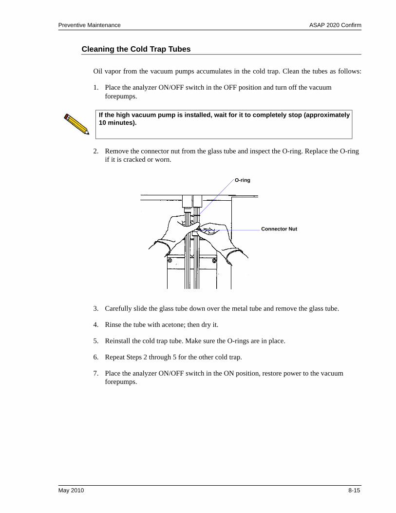
Preventive Maintenance ASAP 2020 Confirm
Cleaning the Cold Trap Tubes
Oil vapor from the vacuum pumps accumulates in the cold trap. Clean the tubes as follows:
1. Place the analyzer ON/OFF switch in the OFF position and turn off the vacuum forepumps.
2. Remove the connector nut from the glass tube and inspect the O-ring. Replace the O-ring if it is cracked or worn.
3. Carefully slide the glass tube down over the metal tube and remove the glass tube.
4. Rinse the tube with acetone; then dry it.
5. Reinstall the cold trap tube. Make sure the O-rings are in place.
6. Repeat Steps 2 through 5 for the other cold trap.
7. Place the analyzer ON/OFF switch in the ON position, restore power to the vacuum forepumps.
If the high vacuum pump is installed, wait for it to completely stop (approximately 10 minutes).
O-ring
Connector Nut
May 2010 8-15
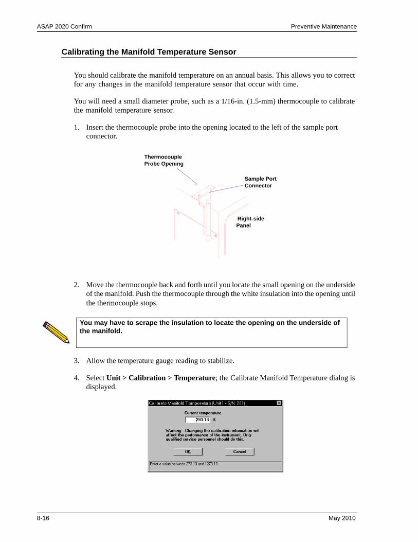
ASAP 2020 Confirm Preventive Maintenance
Calibrating the Manifold Temperature Sensor
You should calibrate the manifold temperature on an annual basis. This allows you to correct for any changes in the manifold temperature sensor that occur with time.
You will need a small diameter probe, such as a 1/16-in. (1.5-mm) thermocouple to calibrate the manifold temperature sensor.
1. Insert the thermocouple probe into the opening located to the left of the sample port connector.
2. Move the thermocouple back and forth until you locate the small opening on the underside of the manifold. Push the thermocouple through the white insulation into the opening until the thermocouple stops.
3. Allow the temperature gauge reading to stabilize.
4. Select Unit > Calibration > Temperature; the Calibrate Manifold Temperature dialog is displayed.
Sample Port Connector
Right-side Panel
Thermocouple Probe Opening
You may have to scrape the insulation to locate the opening on the underside of the manifold.
8-16 May 2010

Preventive Maintenance ASAP 2020 Confirm
5. Enter the manifold temperature indicated on the temperature gauge. Click OK to store the new value.
6. Remove the thermocouple probe.
Testing the Analyzer for Leaks
Refer to Appendix D for instructions on testing the ASAP 2020 for leaks.
May 2010 8-17
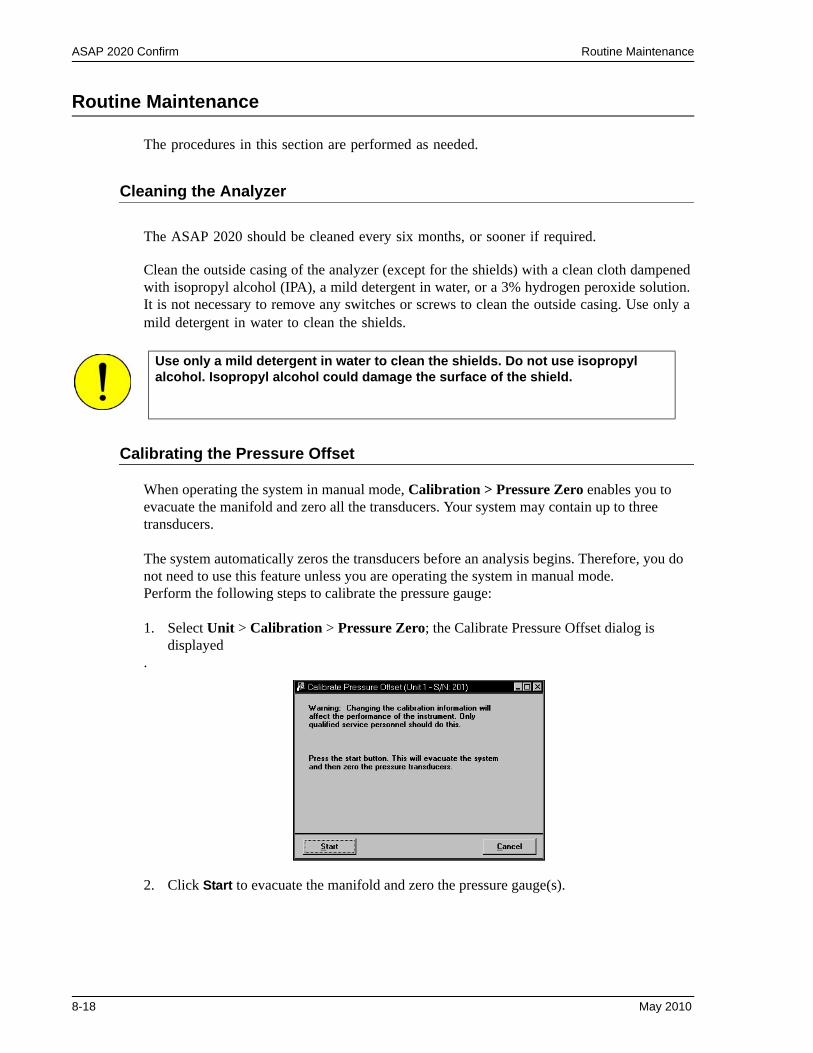
ASAP 2020 Confirm Routine Maintenance
Routine Maintenance
The procedures in this section are performed as needed.
Cleaning the Analyzer
The ASAP 2020 should be cleaned every six months, or sooner if required.
Clean the outside casing of the analyzer (except for the shields) with a clean cloth dampened with isopropyl alcohol (IPA), a mild detergent in water, or a 3% hydrogen peroxide solution. It is not necessary to remove any switches or screws to clean the outside casing. Use only a mild detergent in water to clean the shields.
Calibrating the Pressure Offset
When operating the system in manual mode, Calibration > Pressure Zero enables you to evacuate the manifold and zero all the transducers. Your system may contain up to three transducers.
The system automatically zeros the transducers before an analysis begins. Therefore, you do not need to use this feature unless you are operating the system in manual mode.Perform the following steps to calibrate the pressure gauge:
1. Select Unit > Calibration > Pressure Zero; the Calibrate Pressure Offset dialog is displayed
.
2. Click Start to evacuate the manifold and zero the pressure gauge(s).
Use only a mild detergent in water to clean the shields. Do not use isopropyl alcohol. Isopropyl alcohol could damage the surface of the shield.
8-18 May 2010
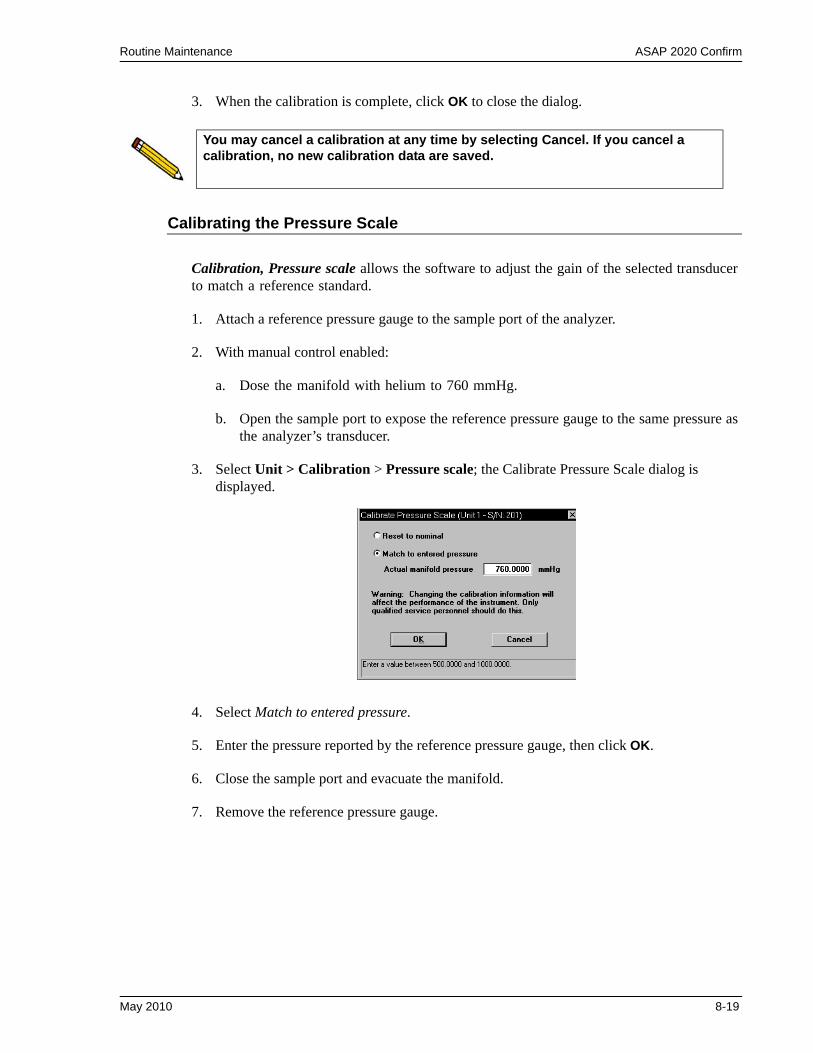
Routine Maintenance ASAP 2020 Confirm
3. When the calibration is complete, click OK to close the dialog.
Calibrating the Pressure Scale
Calibration, Pressure scale allows the software to adjust the gain of the selected transducer to match a reference standard.
1. Attach a reference pressure gauge to the sample port of the analyzer.
2. With manual control enabled:
a. Dose the manifold with helium to 760 mmHg.
b. Open the sample port to expose the reference pressure gauge to the same pressure as the analyzer’s transducer.
3. Select Unit > Calibration > Pressure scale; the Calibrate Pressure Scale dialog is displayed.
4. Select Match to entered pressure.
5. Enter the pressure reported by the reference pressure gauge, then click OK.
6. Close the sample port and evacuate the manifold.
7. Remove the reference pressure gauge.
You may cancel a calibration at any time by selecting Cancel. If you cancel a calibration, no new calibration data are saved.
May 2010 8-19

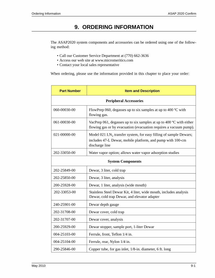
Ordering Information ASAP 2020 Confirm
9. ORDERING INFORMATION
The ASAP2020 system components and accessories can be ordered using one of the follow-ing method:
• Call our Customer Service Department at (770) 662-3636• Access our web site at www.micromeritics.com• Contact your local sales representative
When ordering, please use the information provided in this chapter to place your order:
Part Number Item and Description
Peripheral Accessories
060-00030-00 FlowPrep 060, degasses up to six samples at up to 400 ºC with flowing gas.
061-00030-00 VacPrep 061, degasses up to six samples at up to 400 ºC with either flowing gas or by evacuation (evacuation requires a vacuum pump).
021-00000-00 Model 021 LN2 transfer system, for easy filling of sample Dewars; includes 47-L Dewar, mobile platform, and pump with 100-cm discharge line
202-33050-00 Water vapor option; allows water vapor adsorption studies
System Components
202-25849-00 Dewar, 3 liter, cold trap
202-25850-00 Dewar, 3 liter, analysis
200-25928-00 Dewar, 1 liter, analysis (wide mouth)
202-33053-00 Stainless Steel Dewar Kit, 4 liter, wide mouth, includes analysis Dewar, cold trap Dewar, and elevator adapter
240-25901-00 Dewar depth gauge
202-31708-00 Dewar cover, cold trap
202-31707-00 Dewar cover, analysis
200-25929-00 Dewar stopper, sample port, 1-liter Dewar
004-25103-00 Ferrule, front, Teflon 1/4 in.
004-25104-00 Ferrule, rear, Nylon 1/4 in.
290-25846-00 Copper tube, for gas inlet, 1/8-in. diameter, 6 ft. long
May 2010 9-1
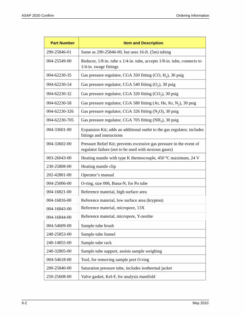
ASAP 2020 Confirm Ordering Information
Part Number Item and Description
290-25846-01 Same as 290-25846-00, but uses 16-ft. (5m) tubing
004-25549-00 Reducer, 1/8-in. tube x 1/4-in. tube, accepts 1/8-in. tube, connects to 1/4-in. swage fittings
004-62230-35 Gas pressure regulator, CGA 350 fitting (CO, H2), 30 psig
004-62230-54 Gas pressure regulator, CGA 540 fitting (O2), 30 psig
004-62230-32 Gas pressure regulator, CGA 320 fitting (CO2), 30 psig
004-62230-58 Gas pressure regulator, CGA 580 fitting (Ar, He, Kr, N2), 30 psig
004-62230-326 Gas pressure regulator, CGA 326 fitting (N2O), 30 psig
004-62230-705 Gas pressure regulator, CGA 705 fitting (NH3), 30 psig
004-33601-00 Expansion Kit; adds an additional outlet to the gas regulator, includes fittings and instructions
004-33602-00 Pressure Relief Kit; prevents excessive gas pressure in the event of regulator failure (not to be used with noxious gases)
003-26043-00 Heating mantle with type K thermocouple, 450 ºC maximum, 24 V
230-25808-00 Heating mantle clip
202-42801-00 Operator’s manual
004-25006-00 O-ring, size 006, Buna-N, for Po tube
004-16821-00 Reference material, high surface area
004-16816-00 Reference material, low surface area (krypton)
004-16843-00 Reference material, micropore, 13X
004-16844-00 Reference material, micropore, Y-zeolite
004-54609-00 Sample tube brush
240-25853-00 Sample tube funnel
240-14855-00 Sample tube rack
240-32805-00 Sample tube support, assists sample weighing
004-54618-00 Tool, for removing sample port O-ring
200-25840-00 Saturation pressure tube, includes isothermal jacket
250-25608-00 Valve gasket, Kel-F, for analysis manifold
9-2 May 2010

Ordering Information ASAP 2020 Confirm
250-25627-00 Valve plunger, Buna-N seal, for analysis manifold
May 2010 9-3
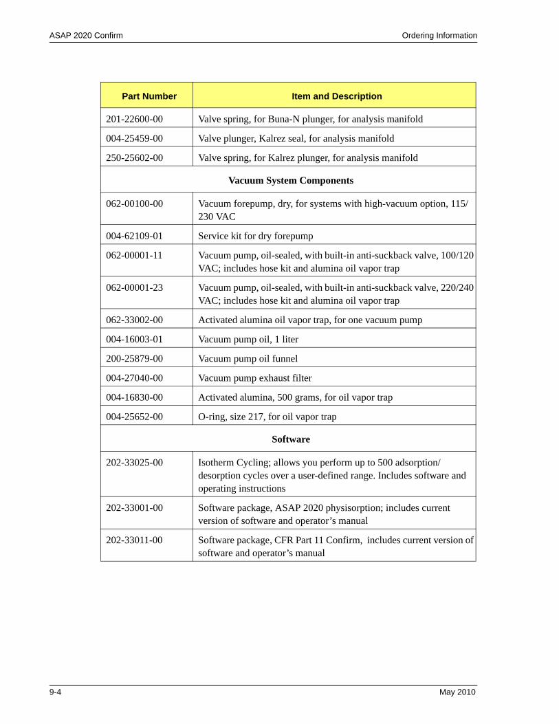
ASAP 2020 Confirm Ordering Information
Part Number Item and Description
201-22600-00 Valve spring, for Buna-N plunger, for analysis manifold
004-25459-00 Valve plunger, Kalrez seal, for analysis manifold
250-25602-00 Valve spring, for Kalrez plunger, for analysis manifold
Vacuum System Components
062-00100-00 Vacuum forepump, dry, for systems with high-vacuum option, 115/230 VAC
004-62109-01 Service kit for dry forepump
062-00001-11 Vacuum pump, oil-sealed, with built-in anti-suckback valve, 100/120 VAC; includes hose kit and alumina oil vapor trap
062-00001-23 Vacuum pump, oil-sealed, with built-in anti-suckback valve, 220/240 VAC; includes hose kit and alumina oil vapor trap
062-33002-00 Activated alumina oil vapor trap, for one vacuum pump
004-16003-01 Vacuum pump oil, 1 liter
200-25879-00 Vacuum pump oil funnel
004-27040-00 Vacuum pump exhaust filter
004-16830-00 Activated alumina, 500 grams, for oil vapor trap
004-25652-00 O-ring, size 217, for oil vapor trap
Software
202-33025-00 Isotherm Cycling; allows you perform up to 500 adsorption/ desorption cycles over a user-defined range. Includes software and operating instructions
202-33001-00 Software package, ASAP 2020 physisorption; includes current version of software and operator’s manual
202-33011-00 Software package, CFR Part 11 Confirm, includes current version of software and operator’s manual
9-4 May 2010
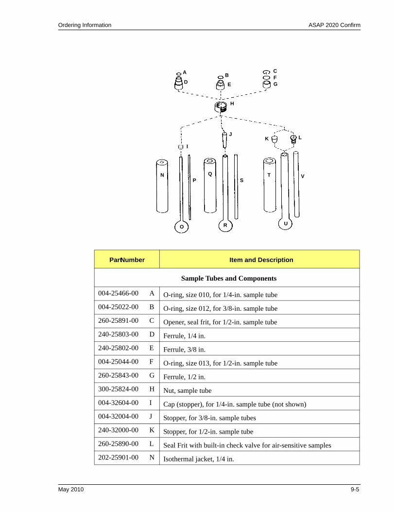
Ordering Information ASAP 2020 Confirm
Part Number Item and Description
Sample Tubes and Components
004-25466-00 A O-ring, size 010, for 1/4-in. sample tube
004-25022-00 B O-ring, size 012, for 3/8-in. sample tube
260-25891-00 C Opener, seal frit, for 1/2-in. sample tube
240-25803-00 D Ferrule, 1/4 in.
240-25802-00 E Ferrule, 3/8 in.
004-25044-00 F O-ring, size 013, for 1/2-in. sample tube
260-25843-00 G Ferrule, 1/2 in.
300-25824-00 H Nut, sample tube
004-32604-00 I Cap (stopper), for 1/4-in. sample tube (not shown)
004-32004-00 J Stopper, for 3/8-in. sample tubes
240-32000-00 K Stopper, for 1/2-in. sample tube
260-25890-00 L Seal Frit with built-in check valve for air-sensitive samples
202-25901-00 N Isothermal jacket, 1/4 in.
A BC
D EFG
H
JK L
N Q T
O
P
R U
SV
I
May 2010 9-5
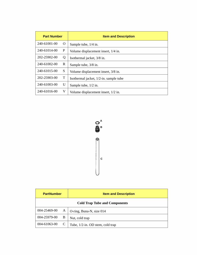
Part Number Item and Description
240-61001-00 O Sample tube, 1/4 in.
240-61014-00 P Volume displacement insert, 1/4 in.
202-25902-00 Q Isothermal jacket, 3/8 in.
240-61002-00 R Sample tube, 3/8 in.
240-61015-00 S Volume displacement insert, 3/8 in.
202-25903-00 T Isothermal jacket, 1/2-in. sample tube
240-61003-00 U Sample tube, 1/2 in.
240-61016-00 V Volume displacement insert, 1/2 in.
Part Number Item and Description
Cold Trap Tube and Components
004-25469-00 A O-ring, Buna-N, size 014
004-25979-00 B Nut, cold trap
004-61063-00 C Tube, 1/2-in. OD stem, cold trap
A
B
C

Ordering Information ASAP 2020 Confirm
May 2010 9-7

ASAP 2020 Confirm Ordering Information
9-8 May 2010

ASAP 2020 confirm Developer/Analyst Operator’s Manual Appendix A
A. FORMS
This appendix contains the following form:
• Sample Data Worksheet
Copy and use this form as needed.
Oct 03 A-1

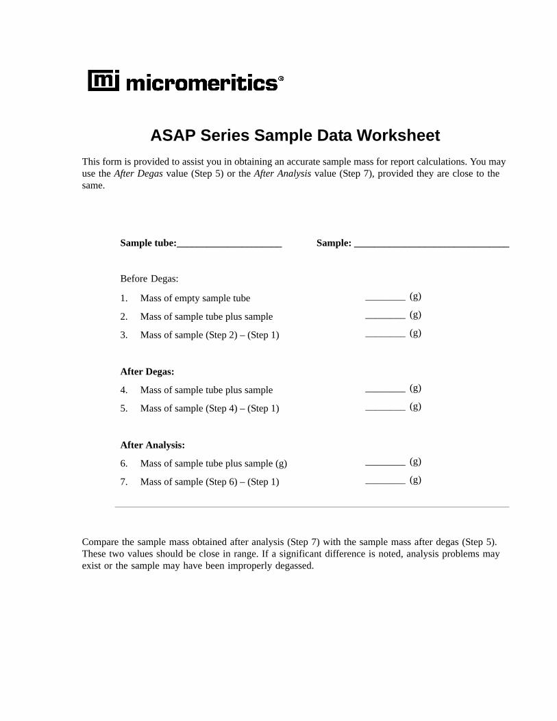
ASAP Series Sample Data WorksheetThis form is provided to assist you in obtaining an accurate sample mass for report calculations. You may use the After Degas value (Step 5) or the After Analysis value (Step 7), provided they are close to the same.
Compare the sample mass obtained after analysis (Step 7) with the sample mass after degas (Step 5). These two values should be close in range. If a significant difference is noted, analysis problems may exist or the sample may have been improperly degassed.
Sample tube:_____________________ Sample: _______________________________
Before Degas:
1. Mass of empty sample tube ________ (g)
2. Mass of sample tube plus sample ________ (g)
3. Mass of sample (Step 2) – (Step 1) ________ (g)
After Degas:
4. Mass of sample tube plus sample ________ (g)
5. Mass of sample (Step 4) – (Step 1) ________ (g)
After Analysis:
6. Mass of sample tube plus sample (g) ________ (g)
7. Mass of sample (Step 6) – (Step 1) ________ (g)

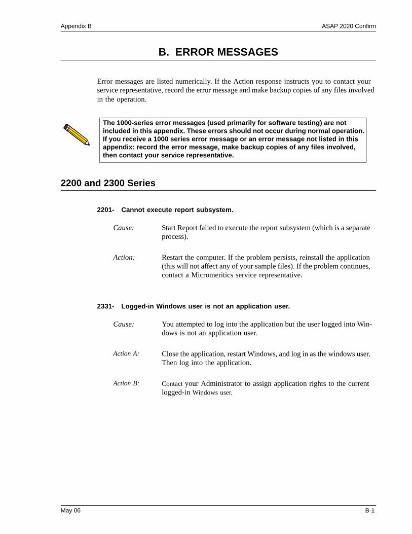
Appendix B ASAP 2020 Confirm
B. ERROR MESSAGES
Error messages are listed numerically. If the Action response instructs you to contact your service representative, record the error message and make backup copies of any files involved in the operation.
2200 and 2300 Series
2201- Cannot execute report subsystem.
2331- Logged-in Windows user is not an application user.
The 1000-series error messages (used primarily for software testing) are not included in this appendix. These errors should not occur during normal operation. If you receive a 1000 series error message or an error message not listed in this appendix: record the error message, make backup copies of any files involved, then contact your service representative.
Cause: Start Report failed to execute the report subsystem (which is a separate process).
Action: Restart the computer. If the problem persists, reinstall the application (this will not affect any of your sample files). If the problem continues, contact a Micromeritics service representative.
Cause: You attempted to log into the application but the user logged into Win-dows is not an application user.
Action A: Close the application, restart Windows, and log in as the windows user. Then log into the application.
Action B: Contact your Administrator to assign application rights to the current logged-in Windows user.
May 06 B-1
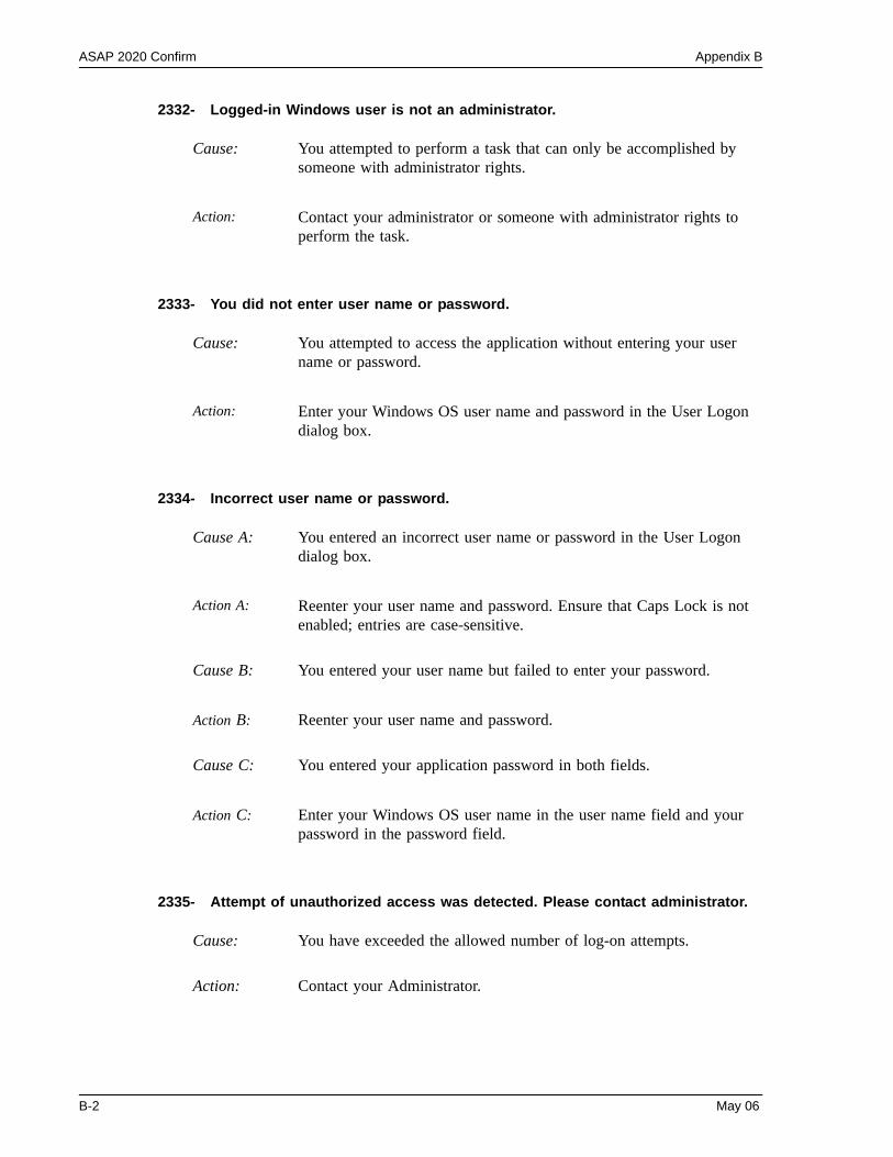
ASAP 2020 Confirm Appendix B
2332- Logged-in Windows user is not an administrator.
2333- You did not enter user name or password.
2334- Incorrect user name or password.
2335- Attempt of unauthorized access was detected. Please contact administrator.
Cause: You attempted to perform a task that can only be accomplished by someone with administrator rights.
Action: Contact your administrator or someone with administrator rights to perform the task.
Cause: You attempted to access the application without entering your user name or password.
Action: Enter your Windows OS user name and password in the User Logon dialog box.
Cause A: You entered an incorrect user name or password in the User Logon dialog box.
Action A: Reenter your user name and password. Ensure that Caps Lock is not enabled; entries are case-sensitive.
Cause B: You entered your user name but failed to enter your password.
Action B: Reenter your user name and password.
Cause C: You entered your application password in both fields.
Action C: Enter your Windows OS user name in the user name field and your password in the password field.
Cause: You have exceeded the allowed number of log-on attempts.
Action: Contact your Administrator.
B-2 May 06
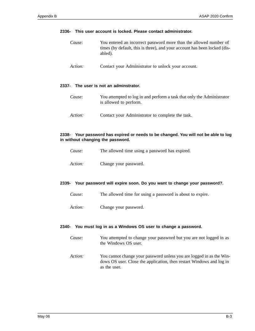
Appendix B ASAP 2020 Confirm
2336- This user account is locked. Please contact administrator.
2337- The user is not an adminstrator.
2338- Your password has expired or needs to be changed. You will not be able to log in without changing the password.
2339- Your password will expire soon. Do you want to change your password?.
2340- You must log in as a Windows OS user to change a password.
Cause: You entered an incorrect password more than the allowed number of times (by default, this is three), and your account has been locked (dis-abled).
Action: Contact your Administrator to unlock your account.
Cause: You attempted to log in and perform a task that only the Administrator is allowed to perform.
Action: Contact your Administrator to complete the task.
Cause: The allowed time using a password has expired.
Action: Change your password.
Cause: The allowed time for using a password is about to expire.
Action: Change your password.
Cause: You attempted to change your password but you are not logged in as the Windows OS user.
Action: You cannot change your password unless you are logged in as the Win-dows OS user. Close the application, then restart Windows and log in as the user.
May 06 B-3
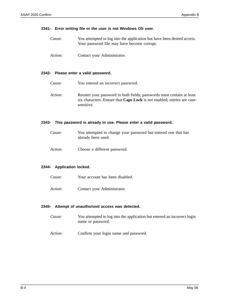
ASAP 2020 Confirm Appendix B
2341- Error writing file or the user is not Windows OS user.
2342- Please enter a valid password.
2343- This password is already in use. Please enter a valid password.
2344- Application locked.
2345- Attempt of unauthorized access was detected.
Cause: You attempted to log into the application but have been denied access. Your password file may have become corrupt.
Action: Contact your Administrator.
Cause: You entered an incorrect password.
Action: Reenter your password in both fields; passwords must contain at least six characters. Ensure that Caps Lock is not enabled; entries are case-sensitive.
Cause: You attempted to change your password but entered one that has already been used.
Action: Choose a different password.
Cause: Your account has been disabled.
Action: Contact your Administrator.
Cause: You attempted to log into the application but entered an incorrect login name or password.
Action: Confirm your login name and password.
B-4 May 06

Appendix B ASAP 2020 Confirm
2346- This user account is disabled. Please contact an administrator.
Cause: You have attempted to log into the application repeatedly but all attempts have failed.
Action: Contact your Administrator.
May 06 B-5
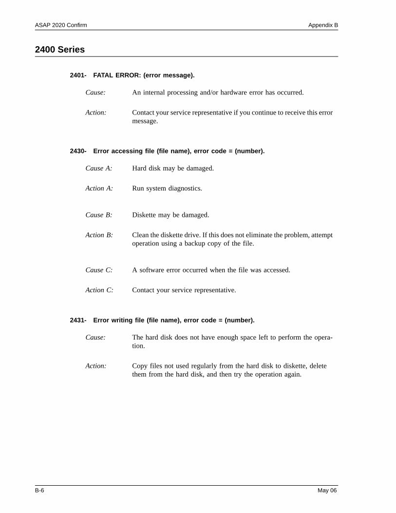
ASAP 2020 Confirm Appendix B
2400 Series
2401- FATAL ERROR: (error message).
2430- Error accessing file (file name), error code = (number).
2431- Error writing file (file name), error code = (number).
Cause: An internal processing and/or hardware error has occurred.
Action: Contact your service representative if you continue to receive this error message.
Cause A: Hard disk may be damaged.
Action A: Run system diagnostics.
Cause B: Diskette may be damaged.
Action B: Clean the diskette drive. If this does not eliminate the problem, attempt operation using a backup copy of the file.
Cause C: A software error occurred when the file was accessed.
Action C: Contact your service representative.
Cause: The hard disk does not have enough space left to perform the opera-tion.
Action: Copy files not used regularly from the hard disk to diskette, delete them from the hard disk, and then try the operation again.
B-6 May 06
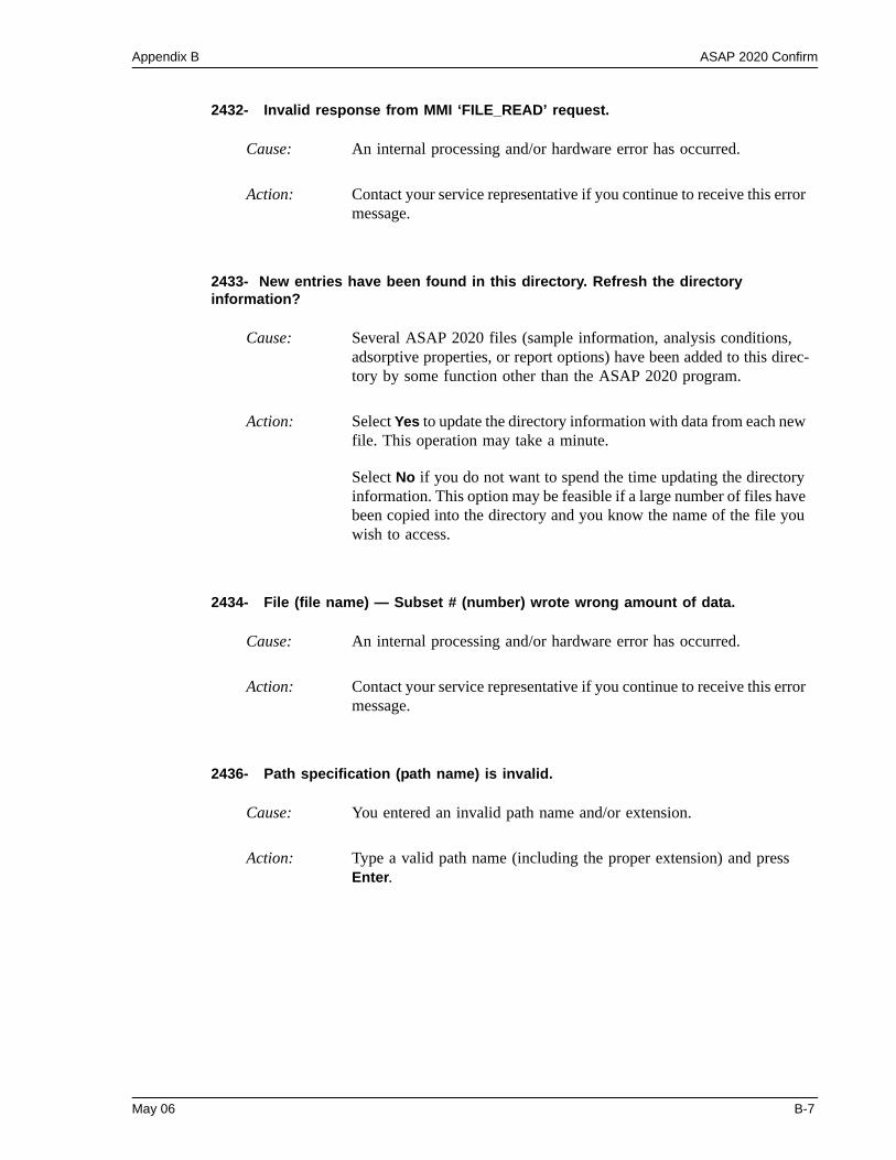
Appendix B ASAP 2020 Confirm
2432- Invalid response from MMI ‘FILE_READ’ request.
2433- New entries have been found in this directory. Refresh the directory information?
2434- File (file name) — Subset # (number) wrote wrong amount of data.
2436- Path specification (path name) is invalid.
Cause: An internal processing and/or hardware error has occurred.
Action: Contact your service representative if you continue to receive this error message.
Cause: Several ASAP 2020 files (sample information, analysis conditions, adsorptive properties, or report options) have been added to this direc-tory by some function other than the ASAP 2020 program.
Action: Select Yes to update the directory information with data from each new file. This operation may take a minute.
Select No if you do not want to spend the time updating the directory information. This option may be feasible if a large number of files have been copied into the directory and you know the name of the file you wish to access.
Cause: An internal processing and/or hardware error has occurred.
Action: Contact your service representative if you continue to receive this error message.
Cause: You entered an invalid path name and/or extension.
Action: Type a valid path name (including the proper extension) and press Enter.
May 06 B-7
ASAP 2020 Confirm Appendix B
2437- File (file name) does not exist.
2438- Disk drive (letter): is inaccessible.
2439- Could not register file.2440- Subset not found.2441- Seek within file failed.2442- Bad header in subset file.2443- Subset owner denied access.2444- Not a valid file format.2445- Subset wrote the wrong amount of data.2446- Error reading data.2447- Error writing data.
2448- File directory (path name) is invalid. Resetting to the installation directory.
2449- This field does not contain a valid file specification.
Cause: You entered a file specification that does not exist.
Action: Enter an existing file specification or select a file name from the list box.
Cause: You selected a disk drive that is not presently accessible.
Action: Ensure that the disk is not write-protected.
Cause: An unexpected error occurred when you tried to access a data file.
Action: Contact your service representative.
Cause: A working directory specified in the .INI file is invalid. The directory may have been deleted or moved to a different location.
Action: The installation directory will be substituted. The next time you open a file, use the Directories: list to move to the correct directory.
Cause: You entered an invalid file name.
Action: See the description of file naming conventions in your DOS or Win-dows manual and re-enter the name.
B-8 May 06
Appendix B ASAP 2020 Confirm
2450- Sample Defaults may not be edited while this operation is in progress. Do you wish to save and close the Sample Defaults edit session?
2452- Attempt to write MICATTR.DIR in read only mode. (file name)2453- Attempt to append MICATTR.DIR in read only mode. (file name)
2454- Too many selections for a print-to-file operation. Only the first (number) selec-tions will be processed. Please reselect the remainder.
2455- Too many selections for an export-to-file operation. Only the first (number) selections will be processed. Please reselect the remainder.
2456- Insufficient file handles available. Application cannot continue.
Cause: You are in the process of initiating an automatic analysis (an analysis in which sample files are created using the defaults) while editing the defaults.
Action: Finish your edit session of the defaults and close the dialog. Then restart the automatic analysis.
Cause: The Read-Only attribute is turned on in the application’s MICATTR.DIR file (this file exists in each folder containing sample or parameter files).
Action: Use Windows Explorer to access the folder containing the MICATTR.DIR file and disable the Read-Only option.
Cause: You selected too many files for this operation.
Action: Select only the number of files specified in the message.
Cause: You have more than 50 files open at the same time.
Action: Refer to the manual for your operating system and set the limit for open files to 50 or greater.
May 06 B-9
ASAP 2020 Confirm Appendix B
2457- Results cannot be displayed. More than (number) windows are currently dis-playing or printing results.
2458- An instrument is performing a critical operation. Wait a few moments before exiting the application.
2459- An instrument is busy. A delay in restarting this application could result in loss of new data. Continue with program Exit?
2460- Fatal Communications error on (unit nn).
Cause: You have too many windows open in the application.
Action: Close some of the open windows.
Cause: You attempted to exit the application while the analyzer is performing a critical operation. This operation must be completed before the appli-cation can be stopped.
Action: Wait a few minutes before attempting to exit the application again.
Cause: You attempted to exit the application while the analyzer was perform-ing an operation.
Action: Rather than exiting the application you may choose to minimize it.
Cause: Repeated attempts to maintain communication with the analyzer have failed.
Action: Check the communications cable connecting the analyzer to the com-puter. Confirm that the analyzer is turned on and that the status light is not blinking.
If these checks are okay, exit the analysis program and then restart the application. If this error persists, contact your service representative.
B-10 May 06
Appendix B ASAP 2020 Confirm
2461- No instruments are in operation. This application will unconditionally terminate.
2471- Unit n - S/N; nn has an invalid communications port specified. It cannot be initialized.
2474- (Unit {number}) Communications port COM (port number) specified in the pro-gram control files is already in use. Unit cannot initialize.
Cause: At least one analyzer must be active for the application to operate. The initialization of the analyzers configured with the Setup program has failed. The application stops.
Action A: Usually this message is preceded by another message giving the reason for the analyzer’s failure to initialize. See the instructions for that mes-sage.
Action B: Check the cable connection between the analyzer and the computer. Verify that the analyzer has the power switch in the ON position and that the light on the front panel is illuminated. If the application con-tinues to fail in its attempts to initialize the analyzer, contact your ser-vice representative.
Cause: The communications port specified for this analyzer during installation (or configuration) is invalid.
Action: Use the setup program to change the analyzer configuration.
Cause: The communications port assigned to the indicated unit is in use by another program.
Action: End the program using the busy port or use the Setup program to change the communications port assigned to this program.
May 06 B-11
ASAP 2020 Confirm Appendix B
2475- (Unit {number}) Communications port COM (port number) specified in the pro-gram control files cannot be accessed. Unit cannot initialize.
2476- Unit startup failed. Cannot initialize the communications port.
2477- (Unit n; Serial nn) did not properly initialize.
2478- Error copying sequential data segment.
Cause: The operating system has prevented the application from accessing the communications port.
Action: Review the hardware configuration of the computer, ensure that no other application is using the port. Contact your service representative if you continue to receive this error message.
Cause: The communications port specified during installation is invalid.
Action: Use the setup program to change the analyzer configuration. Contact your service representative if you continue to receive this error mes-sage.
Cause: The software was unable to initialize the analyzer.
Action A: Run the Setup program and ensure that a valid port is specified; if not, specify a valid one when prompted.
Action B: Reinstall the software, then restart application.
Action C: Contact your Micromeritics service representative if you continue to get this message.
Cause: An internal processing and/or hardware error occurred while accessing a portion of a sample file.
Action: Confirm that the media being accessed does not contain errors; for example, you may wish to use a utility such as ScanDisk. Contact your service representative if you continue to receive this error message.
B-12 May 06
Appendix B ASAP 2020 Confirm
2479- (Unit n; Serial nn) The instrument is busy performing an operation of which this application is unaware. Do you want to cancel? (Yes, No)
2480- File (file name) cannot be analyzed. It is currently being edited.
2481- Error accessing the sample information file (file name).
Cause: During initialization of the application, the status of the analyzer was found to be in a different state than expected.
Action: Click Yes to cancel the operation in process, allowing the analyzer to reset and continue with initialization.
Click No to cancel the initialization process.
If you continue to get this message, verify that files in the application directory structure are not being changed or removed.
Cause: You attempted an analysis using a sample file that is being edited.
Action: Save the changes and close the dialog box.
Cause A: You attempted to open a file that is already open, possibly minimized.
Action A: View the minimized icons, locate and maximize the file.
Cause B: Diskette may be damaged.
Action B: Clean the diskette drive. If this does not eliminate the problem, attempt operation using a backup copy of the file.
Cause C: Hard disk may be damaged.
Action C: Contact your service representative.
Cause D: A software error occurred when the file was accessed.
Action D: Contact your service representative.
May 06 B-13
ASAP 2020 Confirm Appendix B
2482- File cannot be opened for writing. It is already in use.
2483- An analysis cannot be performed on (file name). It is open for editing and con-tains errors.
2484- The edit session for (file name) must be saved before the analysis. Save changes and continue with the analysis.
2485- The service test file has an invalid status and cannot be used for this analysis.
2486- Cannot construct (name) report type. Program will terminate.2487- Cannot start report generator. Error code (number). Program will terminate.
Cause: You are attempting to open a file that is currently being used (either by this application or another).
Action: Locate the application using the file (in the Micromeritics application, use the Windows menu item to get a list of all windows, one of which may contain this file).
Cause: You attempted to use a sample file containing errors that is currently open.
Action: Go to the window containing the file, correct the errors, and save it.
Cause: You attempted an analysis using a sample file that contains unsaved changes.
Action: Select Yes to save the changes and continue with the analysis.
Select No to abort the analysis and return to the sample file.
Cause: The selected service test file has a status other than No Analysis.
Action: Select a different service test file or create a new one and use Replace All to copy parameters from the file you originally selected.
Cause: An internal processing and/or hardware error has occurred.
Action: Contact your service representative if you continue to receive this error message.
B-14 May 06
Appendix B ASAP 2020 Confirm
2488- File (file name) cannot be opened for editing. It is already in use.
2489- File (file name) cannot be opened for writing. It is already in use.
2490- No ‘.INI’ file present. Application will terminate.
2491- Highlighted fields contain errors. Please correct the errors before closing dia-log box.
2492- This field’s entry is INVALID.
2493- An entry is required for this field.
Cause: The file you specified is being used in another edit operation.
Action: Check the Windows list to locate the other edit session.
Cause: The file you specified in a Save As operation is already open for edit.
Action: Select a different file for the Save As operation.
Cause: The ASCII file containing initialization information and system options information used during program startup does not exist.
Action: Run the ASAP 2020 Setup program, select Change analyzer setup, and create the control file used by the ASAP 2020.
Cause: The highlighted fields contain invalid entries. You will not be able to close the dialog box until you correct the errors.
Action: Check the entries, correct the errors, and close the dialog box
Cause: The highlighted field contains an invalid entry.
Action: Check the entry and correct the error.
Cause: This field requires a valid entry for you to proceed.
Action: Enter or select an appropriate value.
May 06 B-15
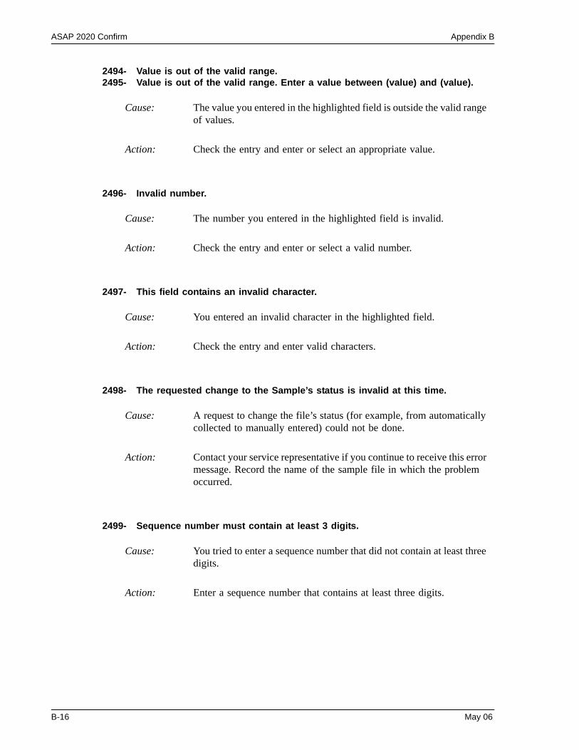
ASAP 2020 Confirm Appendix B
2494- Value is out of the valid range.2495- Value is out of the valid range. Enter a value between (value) and (value).
2496- Invalid number.
2497- This field contains an invalid character.
2498- The requested change to the Sample’s status is invalid at this time.
2499- Sequence number must contain at least 3 digits.
Cause: The value you entered in the highlighted field is outside the valid range of values.
Action: Check the entry and enter or select an appropriate value.
Cause: The number you entered in the highlighted field is invalid.
Action: Check the entry and enter or select a valid number.
Cause: You entered an invalid character in the highlighted field.
Action: Check the entry and enter valid characters.
Cause: A request to change the file’s status (for example, from automatically collected to manually entered) could not be done.
Action: Contact your service representative if you continue to receive this error message. Record the name of the sample file in which the problem occurred.
Cause: You tried to enter a sequence number that did not contain at least three digits.
Action: Enter a sequence number that contains at least three digits.
B-16 May 06
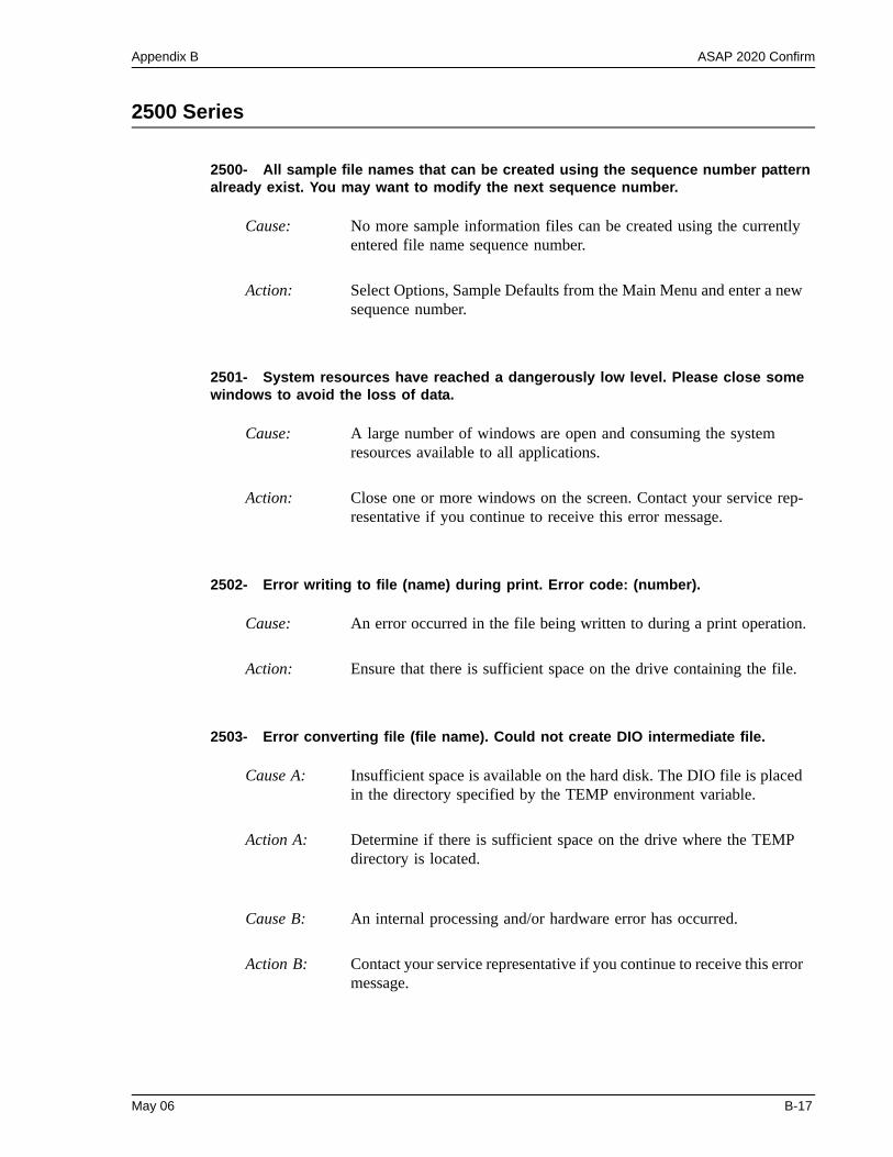
Appendix B ASAP 2020 Confirm
2500 Series
2500- All sample file names that can be created using the sequence number pattern already exist. You may want to modify the next sequence number.
2501- System resources have reached a dangerously low level. Please close some windows to avoid the loss of data.
2502- Error writing to file (name) during print. Error code: (number).
2503- Error converting file (file name). Could not create DIO intermediate file.
Cause: No more sample information files can be created using the currently entered file name sequence number.
Action: Select Options, Sample Defaults from the Main Menu and enter a new sequence number.
Cause: A large number of windows are open and consuming the system resources available to all applications.
Action: Close one or more windows on the screen. Contact your service rep-resentative if you continue to receive this error message.
Cause: An error occurred in the file being written to during a print operation.
Action: Ensure that there is sufficient space on the drive containing the file.
Cause A: Insufficient space is available on the hard disk. The DIO file is placed in the directory specified by the TEMP environment variable.
Action A: Determine if there is sufficient space on the drive where the TEMP directory is located.
Cause B: An internal processing and/or hardware error has occurred.
Action B: Contact your service representative if you continue to receive this error message.
May 06 B-17
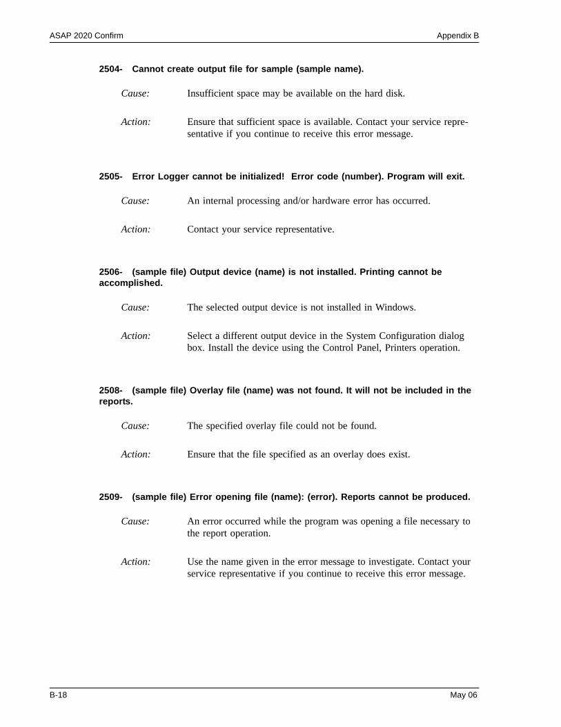
ASAP 2020 Confirm Appendix B
2504- Cannot create output file for sample (sample name).
2505- Error Logger cannot be initialized! Error code (number). Program will exit.
2506- (sample file) Output device (name) is not installed. Printing cannot be accomplished.
2508- (sample file) Overlay file (name) was not found. It will not be included in the reports.
2509- (sample file) Error opening file (name): (error). Reports cannot be produced.
Cause: Insufficient space may be available on the hard disk.
Action: Ensure that sufficient space is available. Contact your service repre-sentative if you continue to receive this error message.
Cause: An internal processing and/or hardware error has occurred.
Action: Contact your service representative.
Cause: The selected output device is not installed in Windows.
Action: Select a different output device in the System Configuration dialog box. Install the device using the Control Panel, Printers operation.
Cause: The specified overlay file could not be found.
Action: Ensure that the file specified as an overlay does exist.
Cause: An error occurred while the program was opening a file necessary to the report operation.
Action: Use the name given in the error message to investigate. Contact your service representative if you continue to receive this error message.
B-18 May 06
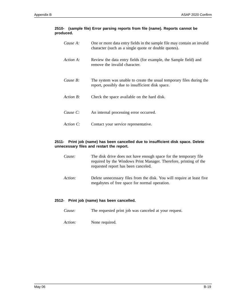
Appendix B ASAP 2020 Confirm
2510- (sample file) Error parsing reports from file (name). Reports cannot be produced.
2511- Print job (name) has been cancelled due to insufficient disk space. Delete unnecessary files and restart the report.
2512- Print job (name) has been cancelled.
Cause A: One or more data entry fields in the sample file may contain an invalid character (such as a single quote or double quotes).
Action A: Review the data entry fields (for example, the Sample field) and remove the invalid character.
Cause B: The system was unable to create the usual temporary files during the report, possibly due to insufficient disk space.
Action B: Check the space available on the hard disk.
Cause C: An internal processing error occurred.
Action C: Contact your service representative.
Cause: The disk drive does not have enough space for the temporary file required by the Windows Print Manager. Therefore, printing of the requested report has been canceled.
Action: Delete unnecessary files from the disk. You will require at least five megabytes of free space for normal operation.
Cause: The requested print job was canceled at your request.
Action: None required.
May 06 B-19
ASAP 2020 Confirm Appendix B
2513- Unable to read the calibration file (file name).
2514- Unable to write the calibration file (file name).
2515- Warning: Changing the calibration information will affect the performance of the instrument. Only qualified service personnel should do this. Do you wish to proceed?
2516- Warning: Keeping a backup copy of the calibration data is recommended by Micromeritics. Would you like to do so now?
2517- Canceling this dialog will reset the calibration state to what it was when this dialog was first opened. Are you sure you want to cancel?
Cause: You selected an invalid calibration file or one that cannot be read.
Action: Be sure the media containing the alleged calibration file has no prob-lems.
Cause: An attempt to Save calibration data has failed due to possible media problems.
Action A: Be sure the media containing the alleged calibration file has no prob-lems.
Action B: Choose an alternate media to Save the calibration data.
Cause: You have started the process of performing a calibration operation.
Action: Calibration operations should only be done by or under the direction of qualified service personnel.
Cause: You have performed a calibration operation; a backup copy is recom-mended.
Action: Perform a calibration Save operation.
Cause: You have not accepted the calibration you performed.
Action: If the calibration operation was successful, press Accept.
B-20 May 06
Appendix B ASAP 2020 Confirm
2521- Unable to program controller.
2522- Invalid controller application file.
2523- Programming the controller failed.2524- CRC check failed on programming controller.2525- Unknown error programming controller.2526- Controller download was not successful.2527- Controller CRC error on boot block.2528- Controller DRAM error.2529- Controller Com1: error.2530- Controller Com2: error.2531- Controller debug port error.
2532- The instrument contains a different software version. Do you want to reset it?
2533- Analyzer initialization failed.
Cause: A hardware malfunction has occurred.
Action: Contact your local Micromeritics service representative.
Cause: The application’s control file has been corrupted or deleted.
Action: Reinstall the ASAP 2020 analysis program.
Cause: An internal processing and/or hardware error has occurred.
Action: Contact your service representative if you continue to receive this error message.
Cause: The application has discovered a different version of software operat-ing in the analyzer.
Action: If there are no analyzers other than the ASAP 2020 connected to the computer, select Yes and allow the updated software to load.
Cause: An internal processing and/or hardware error has occurred.
Action: Contact your service representative if you continue to receive this error message.
May 06 B-21
ASAP 2020 Confirm Appendix B
2534- Error opening file (name) for printing. Error code: (number).
2535- The requested directory is not a repository location. Resetting to the default location.
2536- The maximum number of versions has already been created for this file.
2537- The directory (name) has already been added to the repository.
2538- The archive location name (name) has already been used.
Cause: An error occurred in the selected file for print output.
Action: Ensure that sufficient space is available on the drive containing the file.
Cause: The directory last accessed is no longer available; the application defaults to the default location.
Action: Choose an appropriate directory to select a file.
Cause: The current file contains the maximum number of 676 versions.
Action: If additional versions are required, select File, Save As to create a new file from the current version.
Cause: An internal conflict with the repository structure has occurred.
Action: Contact your Micromeritics service representative.
Cause: An internal conflict with the repository structure has occurred.
Action: Contact your Micromeritics service representative.
B-22 May 06
Appendix B ASAP 2020 Confirm
2539- The repository location (name) cannot be created.
2540- Error getting log file name.
2541- Windows and application user’s rights conflict.
2542- The file (name) could not be written. Check that the directory permissions are correct.
2543- Cannot read from the repository. Check that the directory permissions are correct.
Cause: You attempted to create a new directory (category) or subdirectory (sub-category) but the directory-creating function of the Windows operating system has prevented you from doing so.
Action: Contact your Administrator to review security permissions and local disk space.
Cause: The Confirm application was unable to access (or create) the system log.
Action: Contact your Administrator to review user rights and local disk space.
Cause: You attempted to log into the application, but the windows user rights and Confirm application rights do not agree.
Action: Contact your Administrator to review user rights.
Cause: The system has prevented you from saving your file.
Action: Contact your Administrator to review user rights and local disk space.
Cause: The system has prevented you from accessing a file in the repository.
Action: Contact your Administrator to review user rights for the application and the Windows operating system.
May 06 B-23
ASAP 2020 Confirm Appendix B
2544- Cannot write to the repository. Check that the directory permissions are correct
2545- The repository appears to be empty. Check that the directory permissions are correct.
2546- The file list for the current repository location is missing. Contact an adminis-trator to update the list.
2549- Error accessing online manual file (name).
Cause: The system has prevented you from saving your file to the repository.
Action: Contact your Administrator to review user rights for the application and the Windows operating system.
Cause: The application was unable to determine the repository structure.
Action: Contact your Administrator to review user rights and local disk space.
Cause: You attempted to access a file but the repository does not contain any files.
Action: Contact your Administrator to review user rights and local disk space.
Cause: You were unable to access the operator’s manual.
Action: Reinstall the software. If the problem persists, contact your local Micromeritics service representative.
B-24 May 06
Appendix B ASAP 2020 Confirm
4000 Series
4000- Memory Allocation Error.
4002- Thermal Transpiration correction had no effect.
4003- Error Converting Pressures.4004- Error Computing Volume Adsorbed.
4005- Pressures were not smoothed. Not enough pressures below 0.10 P/Po.
Cause: An internal processing and/or hardware error occurred during report generation.
Action: Contact your service representative if you continue to receive this error message.
Cause: The Thermal transpiration correction option was selected on the Report Options dialog box. However, the correction did not change any pres-sure by more than one percent.
Action: De-select this option to disable this message. This correction is only meaningful for very low pressures.
Cause: An internal processing and/or hardware error occurred during report generation.
Action: Contact your service representative if you continue to receive this error message.
Cause: The Smooth pressures below 0.10 P/Po option was selected on the Report Options dialog. There must be at least 10 pressures within this range for smoothing to occur.
Action: Deselect this option to disable this message.
May 06 B-25
ASAP 2020 Confirm Appendix B
4006- Report Type Not Found.4007- Error Processing Report.
4008- Report requested on sample file with no data points.
4009- Error, No Reports Selected.
4010- Summary Report was not included in the Selected Reports.
Cause: An internal processing and/or hardware error occurred during report generation.
Action: Contact your service representative if you continue to receive this error message.
Cause: You selected a file for reporting which contains no collected data.
Action: Select another file which contains collected data and restart the report.
Cause: You attempted to generate reports for a sample that has no reports selected in its report options.
Action: Select the desired reports in the sample’s report options and save the sample file.
Cause: You did not select a plot or a table for any of the Selected Reports in the Report Options dialog; you selected the reports only to generate an entry in the summary. However, the Summary was not included in the Selected Reports.
Action: Select a plot or table in one or more of the Selected Reports, and/or add the Summary to the Selected Reports.
B-26 May 06
Appendix B ASAP 2020 Confirm
4011- Analysis gas in sample file does not match any gas in unit.
4012- Psat gas in sample file does not match any gas in unit.
4013- The ‘Incremental Dosing’ option is not available on the selected unit.
4014- File (name) is not a valid file for conversion.
Cause: You attempted to start an analysis using a sample information file in which the analysis gas specified does not match the analysis gas entered in the unit configuration.
Action: If necessary, attach the appropriate gas bottle, then enter the gas in the Unit Configuration dialog box.
Cause: You attempted to start an analysis using a sample information file in which the Psat gas does not match the Psat gas entered in the unit con-figuration.
Action: If necessary, attach the appropriate gas bottle, then enter the gas in the Unit Configuration dialog box.
Cause: The MicroPore option is not installed.
Action: Install the MicroPore option before starting the analysis.
Cause: The file selected for conversion is not a MICMOS 2000 or 2000 MicroPore file.
Action: Select only files that have been created by MICMOS 2000 or 2000 MicroPore programs.
May 06 B-27
ASAP 2020 Confirm Appendix B
4015- Error creating export file for sample <sample file name>.
4016- Sample (file name) has no data for export.
4017- Damage to the instrument will result if the sample has not been manually evac-uated. Have you evacuated the sample?
Cause: A file error occurred during creation of an export output file.
Action: The output file name may be invalid. Ensure that the target directory exists. Ensure that the target diskette is not full or write protected. The target disk drive may be damaged or inoperative. Verify that other files may be created on the same drive. Contact your service representative if you continue to receive this error message.
Cause: The file selected for export has a status of No Analysis. No export file will be created.
Action: Select a file which contains analysis data.
Cause: You did not select Backfill sample at start of analysis on the Sample Backfill Options dialog box. The sample tube is normally at atmo-spheric pressure when an analysis is started, and it must be backfilled before the analysis begins to prevent sample material from being drawn into the manifold.
Action: If you have manually evacuated the sample tube, select Yes. If you have not, select No and then either perform a manual evacuation or go to the Sample Backfill Options dialog box and select Backfill sample at start of analysis.
B-28 May 06
Appendix B ASAP 2020 Confirm
4020- Disabling this option may damage the instrument. Are you sure that the sample should not be backfilled?
4021- The entered Po value (Po and Temperature Options of the Analysis Conditions) is outside the range of the pressures listed in the Psat vs. Temperature Table (Adsorp-tive Properties).
4022- The entered bath temperature value (Po and Temperature Options of the Anal-ysis Conditions) is outside the range of the temperatures listed in the Psat vs. Temperature Table (Adsorptive Properties).
Cause: You did not select Backfill sample at start of analysis on the Sample Backfill Options dialog. The sample tube is normally at atmospheric pressure when an analysis is started; it must be backfilled before the analysis begins to prevent sample material from being drawn into the manifold.
Action: If you want to manually evacuate the sample prior to the start of the analysis, select Yes. Otherwise, select No, go to the Sample Backfill Options dialog, and select Backfill sample at start of analysis.
Cause: The temperature that corresponds to the entered Po cannot be found because the entered Po is outside of the range of values in the Psat vs. T table.
Action A: Enter a Po that is within the range of the table.
Action B: Use a different Psat vs. T table.
Cause: The Po that corresponds to the entered temperature cannot be found because the entered temperature is outside of the range of values in the Psat vs. T table.
Action A: Enter a temperature that is within the range of the table.
Action B: Use a different Psat vs. T table.
May 06 B-29

ASAP 2020 Confirm Appendix B
4023- The file (sample file) cannot be prepared for analysis. It is open for editing and contains errors.
4024- Backfill gas in sample file does not match any gas in unit.
4025- There is no Helium attached to the unit.
4026- Cannot calculate Dubinin-Astkahov: bad least squares data.
4027- Fewer than two sample files have data suitable for heat of adsorption reports.
Cause: You attempted an analysis using a sample file that is being edited and has invalid values in one or more of its fields.
Action: Enter valid values into the fields that have errors, save the changes, and close the dialog box.
Cause: You selected a backfill gas that is not included in the gas configuration.
Action: Make sure that gas selections match the gases that are attached to the instrument. Choose one of the gases as the backfill gas, or edit the sam-ple file and choose one of the existing gases as the backfill gas.
Cause: A measured free space has been requested but Helium does not appear to be available.
Action: Make sure the helium cylinder is attached to the unit at its designated port.
Cause: Less than two selected data points are within the fitted pressure range.
Action: Edit the calculation assignments on the Collected Data dialog, or change the fitted pressure range on the Dubinin report options dialog.
Cause: Less than two of the sample files you selected for heat of adsorption reports contain appropriate data.
Action: Edit the Quantity Adsorbed table, or select other sample files.
B-30 May 06
Appendix B ASAP 2020 Confirm
4028- Dubinin calculations cannot be performed because the affinity coefficient of the analysis gas is zero.
4029- At least two fitted data points are needed for Alpha-S calculations.
4030- Preparations failed in primary data.
4031- Not enough points with a relative pressure in the range (n,n)
4032- Some summary reports could not be produced because they require the Micropore option.
Cause: Dubinin values could not be calculated because the affinity coefficient of the analysis gas is zero.
Action: Access the Dubinin Report Adsorptive options in the sample file and enter an appropriate value for the analysis gas.
Cause: Fewer than two data points fall within the selected Alpha-s range.
Action: Edit the calculation assignments or the fitted Alpha-s range, or use a different reference curve.
Cause: Appropriate data were not available to generate the report.
Action: This message was preceded by a different error message; refer to the cause/action of the preceding message.
Cause: Fewer than two data points selected for the Dubinin report falls within the selected relative pressure range.
Action: Edit the calculation assignments or the fitted relative pressure range.
Cause: Some of the summary reports you requested were not produced because you do not have the micropore option installed.
Action: Edit the summary report and deselect the micropore options.
May 06 B-31
ASAP 2020 Confirm Appendix B
4033- Not enough points to generate Dubinin Tabular Report.
4034- Fewer than 2 points available for Dubinin calculations.
4035- Cannot calculate optimized Astakhov exponent: Not enough points with a rel-ative pressure in the range [(pressure), (pressure)].
4036- Fewer than 2 points available for Horvath-Kawazoe calculations.
Cause: There are fewer than two data points selected for the Dubinin tabular reports.
Action: Examine the calculation assignments in the Collected Data dialog of the sample file. You must have at least two micropore pressures selected for inclusion in the Dubinin report.
Cause: There are fewer than two data points selected for Dubinin reports in one of the sample files selected.
Action: Examine the calculation assignments in the Collected Data dialog of the sample file. You must have at least two micropore pressures selected for inclusion in the Dubinin report.
Cause: There are fewer than two valid data points in the relative pressure range specified. Astakhov reports will not be produced.
Action: Examine the calculation assignments in the Collected Data dialog for the sample file. You must have at least two pressures in the given range selected for inclusion in the Dubinin report.
Cause: You must select at least two data points for inclusion in the Horvath-Kawazoe analysis on the Collected Data dialog. No report will be pro-duced.
Action: From the Collected Data dialog, select the data points to be analyzed.
B-32 May 06
Appendix B ASAP 2020 Confirm
4037- Computations failed while processing the primary data set. No reports will be produced.
4038- Fewer than 2 points available for the Langmuir Qm computation. Cheng/Yang correction will not be applied.
4039- The isotherm does not meet the constraints of the Cheng/Yang assumption. Cheng/Yang correction will not be applied.
Cause: The preparation of data for reporting could not be successfully com-pleted. No Horvath-Kawazoe reports will be produced. This message will always be preceded with another one containing additional infor-mation.
Action: Refer to the number of the error message which preceded this one for an explanation.
Cause: The Cheng/Yang correction to the Horvath-Kawazoe equation requires the value of the monolayer volume as calculated from the Langmuir equation. The isotherm must include at least two points above 0.02 rel-ative pressure for the Langmuir equation to be applied.
Action: The analysis will be performed without the Cheng/Yang correction. Deselect Apply Cheng/Yang correction on the Horvath-Kawazoe Report Options dialog to prevent this message from appearing on future reports.
Cause: The Cheng/Yang correction to the Horvath-Kawazoe equation requires the value of the monolayer volume as calculated from the Langmuir equation. The isotherm does not correlate to the Langmuir assumption with a coefficient of 0.98 or more. The correction is not applicable to this isotherm or to the range of the data points selected.
Action A: The analysis will be performed without the Cheng/Yang correction. Deselect Apply Cheng/Yang correction on the Horvath-Kawazoe Report Options dialog to prevent this message from appearing on future reports.
Action B: Generate the Langmuir report for the same data points selected for the Horvath-Kawazoe report. If the Langmuir correlation coefficient can be brought above 0.98 by removing some points at high relative pres-sure, remove them and reproduce the Horvath-Kawazoe reports.
May 06 B-33
ASAP 2020 Confirm Appendix B
4040- The value of Qm computed from the Langmuir equation is too low. The pore size will not be computed for all data points.
4041- Cheng/Yang correction is inappropriate for some P/Po.
4042- 0.0 cannot be a starting or ending pressure for a geometric progression from low pressure.
Cause: The Cheng/Yang correction to the Horvath-Kawazoe equation requires the value of the monolayer volume as calculated from the Langmuir equation. The computed value is less than the volume adsorbed at the largest relative pressure included in the analysis. The correction is not applicable to this isotherm or to the range of the data points selected.
Action: The analysis will be performed and the Cheng/Yang correction will be applied to all points with a volume adsorbed less than the value of Vm. The pore size will not be calculated for data points with an invalid vol-ume adsorbed. Deselect Apply Cheng/Yang correction on the Horvath-Kawazoe Report Options dialog to clear this message.
Cause: The Cheng/Yang correction is usually inappropriate for any P/Po above the isotherm knee. In some instances, the computed pore sizes may decrease above the knee. While it is possible to include these relative pressures (usually above 0.1 P/Po) in the analysis, the computed pore sizes for these pressures are usually meaningless.
Action: Change the data points selected for the Horvath-Kawazoe report to include only relative pressures at or below the knee of the isotherm, or change the Horvath-Kawazoe report options so that the Cheng/Yang correction is not applied.
Cause: You selected to generate a pressure table from a geometrically pro-gressing range.
Action: Change the 0.0 entered value.
B-34 May 06
Appendix B ASAP 2020 Confirm
4043- 1.0 cannot be a starting or ending pressure for a geometric progression toward saturation.
4044- Points in the Langmuir report pressure table lie outside the collected data.
4045- Points in the report pressure table lie outside the collected data.
4046- (file name) could not be opened for reading.
4047- Warning: An error occurred while reading (file name).
Cause: You selected to generate a pressure table from a geometrically pro-gressing range.
Action: Change the 1.0 entered value.
Cause: Calculation assignments are not being used and more than one of the report pressure table points is above the range of the collected data, and more than one is below.
Action: Change the report pressure table to be more consistent with the col-lected data.
Cause: Calculation assignments are not being used and more than one of the report pressure table points is above the range of the collected data, and more than one is below.
Action: Change the report pressure table to be more consistent with the col-lected data.
Cause: A thickness curve file could not be opened.
Action: If the problem persists, restart your computer and optionally perform a media integrity check (using ScanDisk).
Cause: An error happened during a read operation of a thickness curve file.
Action: If the problem persists, restart your computer and optionally perform a media integrity check (using ScanDisk).
May 06 B-35
ASAP 2020 Confirm Appendix B
4048- Warning: An error occurred while restoring the heat of adsorption report editor.
4049- The sample (file name) does not have enough data. A minimum of two adsorp-tion points is required.
4050- None of the requested quantities adsorbed is within the range of the collected data of more than one sample file.
4051- The sample (file name) does not have any data in the range of the requested quantities adsorbed.
Cause: The state of the heat of adsorption report editor could not be restored. Default settings will be used.
Action: No action.
Cause: A sample file has been included in the Heat of Adsorption report that does not have enough data.
Action: Remove the file from the selected file list.
Cause: The Heat of Adsorption report failed because the specified quantities are not within the range of the collected data.
Action A: Edit the quantities adsorbed so that they are within the range of the col-lected data, or select other sample files.
Cause: The sample’s data cannot be interpolated to any of the quantities adsorbed.
Action: Edit the quantities adsorbed so that they are within the range of the col-lected data.
B-36 May 06
Appendix B ASAP 2020 Confirm
4052- Fewer than two points are selected for this report.
4053- At least two data points must be selected for t-Plot calculations.
4054- Fewer than two data points are inside the fitted thickness range.
4055- The BET surface area could not be calculated.
Cause: At least two points are required for the BET calculations.
Action: Edit the calculation assignments for the BET report.
Cause: At least two points are required for the t-Plot calculations.
Action: Edit the calculation assignments for the t-Plot report.
Cause: At least two points must be within the fitted thickness range for the t-Plot calculations.
Action A: Edit the calculation assignments for the t-Plot report.
Action B: Edit the fitted thickness range in the t-Plot report editor.
Cause: Fewer than two points were assigned to the requested surface area cal-culation in the collected data table.
Action A: Assign more points to the surface area calculation.
Action B: Select a different surface area in the t-Plot report editor.
May 06 B-37
ASAP 2020 Confirm Appendix B
4056- The Langmuir surface area could not be calculated.
4057- At least two data points are needed for Freundlich calculations.
4058- At least two data points are needed for Temkin calculations.
4059- Fewer than 2 points available for MP-Method calculations.
Cause: Fewer than two points were assigned to the requested surface area cal-culation in the collected data table.
Action A: Assign more points to the surface area calculation.
Action B: Select a different surface area in the t-Plot report editor.
Cause: Less than two data points have been selected for the Freundlich report; at least two are required.
Action: Select Freundlich points on the Collected Data dialog. If calculation assignments are not being used, edit the Freundlich Report options, Absolute pressure range in the sample file.
Cause: Less than two data points have been selected for the Temkin report; at least two are required.
Action: Select Temkin points on the Collected Data dialog. If calculation assignments are not being used, edit the Temkin Report options, Abso-lute pressure range in the sample file.
Cause: At least two points are required for the MP-Method calculations.
Action: Edit the calculation assignments for the MP-Method report.
B-38 May 06
Appendix B ASAP 2020 Confirm
4060- Sample (file name) contains no data points.
4061- The t-curve must contain at least 2 points.
4062- Error during report generation.
4063- The data requested on this report are not available.
4064- This report cannot be produced without the Micropore option.
Action: An attempt was made to save a sample without collected data as a t-curve or alpha-S curve.
Cause: Repeat the save as t-curve or save as alpha-S operation after opening a sample that has collected data.
Cause: At least two points are required in a thickness curve definition.
Action: Edit the thickness curve.
Cause: An internal processing error has occurred.
Action: Contact your Micromeritics service representative.
Cause: There is no information in the sample log to report.
Action: You selected a sample file for which no instrument operations have been used. Select a sample file with a status of Prepared, Preparing, Analyzing, or Complete to obtain a valid sample log report.
Cause: You requested a report that requires the micropore option.
Action: Deselect the report. Order the Micropore option to install on teh ana-lyzer.
May 06 B-39
ASAP 2020 Confirm Appendix B
4067- No data points are within the range of pressures in the reference isotherm.
4068- No points were selected for the f-Ratio report.
4069- Dosing method choice is invalid. The Analysis Conditions choice of Absolute pressure dosing requires that the Adsorptive Properties (Dosing Method) is set to Normal.
4070- Unable to load deconvolution model (name).
Cause: Thre are no collected data points within the range of pressures in the reference isotherm.
Action: Select data points that are in the range of the reference isotherm, or select a more appropriate reference isotherm.
Cause: The collected data column for the f-Ratio report does not have any points selected.
Action: Edit the collected data dialog and select points for the f-Ratio report.
Cause: There is an incompatibility between the analysis conditions choice of Absolute pressure dosing and the adsorptive properties dosing method.
Action: Edit one of the choices.
Cause: For some reason, the list of available models was corrupted, therefore, the model selected could not be loaded for the deconvolution.
Action: Exit the program and reinstall the software, then try again.
B-40 May 06
Appendix B ASAP 2020 Confirm
4071- The selected pressures points do not form a valid set for deconvolution.
4072- The range of pressures selected is too small to deconvolute using this model.
4073- The analysis gas (name) does not match the model gas (name).
4076- Invalid sample file - Adsorptive Properties “Non-condensing adsorptive” can-not be used unless Analysis Conditions “Absolute pressure dosing” is selected.
Cause: The data points selected for analysis do not contain enough informa-tion to allow a DFT Plus data reduction.
Action A: Edit data points in the table of the Collected Data dialog, or select another sample file. At least two points with strictly increasing pres-sures and volumes adsorbed are required for a DFT Plus data reduc-tion.
Action B: Edit the pressure range on the DFT report options dialog.
Cause: A null result was found using the selected model.
Action: Edit data points in the table of the Collected Data dialog, or select another sample file. At least two points with strictly increasing pres-sures and volumes adsorbed are required for a DFT Plus data reduc-tion.
Cause: The model assumes a specific gas and the sample file uses a different one.
Action: Select a model that assumes the same gas.
Cause: You selected a sample file that has Non-condensing adsorptive selected in the Adsorptive Properties but does not have Absolute pres-sure dosing selected in Analysis Conditions.
Action A: If you plan to use a non-condensing adsorptive, select Absolute pres-sure dosing on the Analysis Conditions dialog.
Action B: If you are not using a non-condensing adsorptive, deselect the Non-condensing adsorptive option on the Adsorptive Properties dialog, or choose an adsorptive that you are sure in not non-condensing.
May 06 B-41
ASAP 2020 Confirm Appendix B
4077- Cannot get surface area for: (file name)
4078- Slope and Y-Intercept cannot be determined from the selected points.
4079- Points found with negative pressure values will not appear on the graph.
Cause: The Isotherm report for the named overlay file has Per gram selected for the Volume Adsorbed, and the Isotherm report for the primary file has a surface area option selected for the Volume Adsorbed.
Action A: Edit the Isotherm report for the named overlay file and select a surface area option for Volume Adsorbed.
Action B: Click Overlays on the Report options dialog of the primary file and remove the named overlay file from the list.
Cause: The Langmuir report cannot be generated from the selected points.
Action: Edit the calculation assignments in the Langmuir column on the Collected Data dialog.
Cause: Collected data contains negative pressure values.
Action: Negative pressure points are automatically removed from isotherm graphs. If you wish to have negative pressure values appear on the graph: Open the sample file and click the Collected Data tab. Deselect Use calculation assignments and then select the points with negative pressures as Outliers.
B-42 May 06
Appendix B ASAP 2020 Confirm
6200 Series
6201- ‘GetOpenFile()’ reports error code (number). File selection cannot be made.
6202- Invalid communications port (port name) specified in the application’s config-uration settings. Unit cannot initialize.
6203- No serial number available. Unit cannot initialize.
6204- The disk does not have enough room for the ROA data. The space required is (number) megabytes.
Cause: You specified a file name which does not exist.
Action: Confirm that the file name used is valid and that the file exists.
Cause A: The communications port assigned to the ASAP 2020 cannot be made available for proper communications.
Action A: Run the ASAP 2020 Setup program, select Change analyzer setup, and enter the correct port information. If the message continues, contact your service representative.
Cause B: The ASAP 2020 control file was manually modified and an invalid communications port was specified.
Action B: Use the ASAP 2020 Setup program to change the communications port assigned to the ASAP 2020.
Cause: The ASAP 2020 control file does not contain a serial number for the unit.
Action: Run the ASAP 2020 Setup program, select Change analyzer setup, and define the serial number for the instrument.
Cause: The computer’s disk is almost out of disk space.
Action: Delete unwanted files.
May 06 B-43
ASAP 2020 Confirm Appendix B
6206- An error occurred creating the ROA data file (file name). The error code was (n).
6209- Analysis startup failed. (Secondary message number and text.)
6212- Calibrating. This action must be completed before the application exits.
6216- Instrument could not initialize. Reason: (reason).
Cause: A software error occurred when the file was being created.
Action: Contact your Micromeritics service representative.
Cause: The ASAP 2020 Program was unable to start an analysis with the indi-cated unit.
Action: Refer to the specified error number and text for instructions.
Cause: The unit is calibrating.
Action: Do not exit the application until the calibration is complete.
Cause: An internal processing and/or hardware error has occurred.
Action: The specific reason given may identify a possible corrective action. Contact your service representative if you continue to receive this error message.
B-44 May 06
Appendix B ASAP 2020 Confirm
6235- (Unit [number]) Analysis canceled: Time limit exceeded while dosing Psat tube to 925 mmHg.
6237- (Unit [number]) Analysis canceled: Time limit exceeded while evacuating Psat tube.
6240- Leak test failed.
Cause A: A pressure of 925 mmHg was not attained within the allowed time. The Psat gas regulator may be set too low or turned off.
Action A: Set the Psat gas regulator to 10 psig (0.7 bar). Then restart the analysis.
Cause B: The Psat gas bottle is empty.
Action B: Connect a new Psat gas bottle. Then restart the analysis.
Cause C: The Psat tube fitting is loose.
Action C: Check the Psat tube fittings and ensure that the tube is attached securely to the port. Then restart the analysis.
Cause: The maximum time for evacuating the Psat tube was exceeded before the vacuum set point was achieved.
Action: Check the Psat tube fittings. Tighten the connector nut if necessary; then restart the analysis.
Cause: With the sample port valve closed, the sample pressure increased by 0.15 mmHg before the leak test duration was completed.
Action: Check sample tube fitting and ensure that it is securely attached to the port. Then restart the analysis.
May 06 B-45
ASAP 2020 Confirm Appendix B
6241- (Unit [number]) Analysis canceled: Maximum time exceeded before the elevator reached the UP (or DOWN) position.
6244- (Unit [number]) Analysis canceled: Time limit exceeded while storing analysis gas in Psat tube.
Cause A: The maximum time for the analysis was exceeded before the elevator reached the UP (or DOWN) position. Ice may be present in the bottom or the neck of the Dewar.
Action A: Check the Dewar and remove ice if necessary. Refer to Checking the Analysis Port Dewar in Chapter 8. Then restart the analysis.
Cause B: The Psat tube is interfering with elevator movement.
Action B: Make sure the Psat tube is close to the sample tube and the Dewar cover is over both the sample and Psat tubes. Then restart the analysis.
Cause A: The time limit (10 minutes) was exceeded while storing the analysis gas in the Psat tube. The Psat gas regulator may be set too low or turned off.
Action A: Set the Psat gas regulator to 10 psig (0.7 bar). Then restart the analysis.
Cause B: The Psat gas bottle is empty.
Action B: Connect a new Psat gas bottle. Then restart the analysis.
Cause C: The Psat tube fitting is loose.
Action C: Check the Psat tube fittings and ensure that the tube is attached securely to the port. Then restart the analysis.
B-46 May 06
Appendix B ASAP 2020 Confirm
6500 Series
6500- Failed to evacuate manifold to VAC SET in (number of) seconds. Calibration canceled.
6501- The 1000 mmHg transducer offset exceeds recommended limits: (number)
6502- The 10 mmHg transducer offset exceeds recommended limits: (number)
Cause A: The vacuum set point is set too low.
Action A: Ensure that the vacuum set point is at 5.0 mmHg. If the set point is already at 5.0 mmHg or above, the vacuum gauge may need servicing.
Cause B: Leak in manifold.
Action B: Locate the leak and repair it. Refer to Chapter 8, Troubleshooting and Maintenance. Restart calibration.
Cause C: Valve failure.
Action C: Identify the leaking valve. Contact your service representative.
Cause: The Pressure Gauge Calibration operation showed the transducer offset exceeds the recommended limit.
Action: Repeat the Pressure Gauge Calibration operation, if this message occurs again contact a Micromeritics service representative.
Cause: The Pressure Gauge Calibration operation showed the transducer offset exceeds the recommended limit.
Action: Repeat the Pressure Gauge Calibration operation, if this message occurs again contact a Micromeritics service representative.
May 06 B-47
ASAP 2020 Confirm Appendix B
6503- The 1 mmHg transducer offset exceeds recommended limits: (number)
6504- Unable to write the calibration file (name).
6505- Unable to read the calibration file (name).
6506- Calibration file for (file name) is invalid.
6509- The sample has an invalid status and cannot be used for degassing.
Cause: The Pressure Gauge Calibration operation showed the transducer offset exceeds the recommended limit.
Action: Repeat the Pressure Gauge Calibration operation, if this message occurs again contact a Micromeritics service representative.
Cause: A Save to File operation failed.
Action: Confirm there is sufficient free space on the media receiving the file and that the media is not corrupted (run ScanDisk). If the problem per-sists contact a Micromeritics service representative.
Cause: A Load from File operation failed.
Action: Confirm there is sufficient free space on the media receiving the file and that the media is not corrupted (run ScanDisk). If the problem per-sists contact a Micromeritics service representative.
Cause: A Load From File operation failed due to invalid information in the file.
Action: Confirm there is sufficient free space on the media receiving the file and that the media is not corrupted (run ScanDisk). If the problem per-sists contact a Micromeritics service representative.
Cause: A file selected for degassing has a status other then No Analysis or Pre-pared.
Action: Select a different file.
B-48 May 06
Appendix B ASAP 2020 Confirm
6510- Error evacuating.
6511- Error dosing.
6512- Error calibrating the servo.
6513- Error waiting for pressure to drop.
6514- Problem encountered dosing to target [PR2] [PR-U], last pressure = [PR4] [PR-U], elapsed time = [0]:[0].
Cause: An evacuation error occurred during a degas operation.
Action: If the problem persists, contact a Micromeritics service representative.
Cause: A dosing error occurred during a degas operation.
Action: If the problem persists, contact a Micromeritics service representative.
Cause: An error occurred while calibrating the servo valve.
Action: If the problem persists, contact a Micromeritics service representative.
Cause: A pressure error occurred during a degas operation.
Action: If the problem persists, contact a Micromeritics service representative.
Cause: Dosing during an analysis did not come within the allowed range of the target.
Action: Check that the outlet stage of the gas regulator is within specification. If the problem occurs frequently contact a Micromeritics service rep-resentative.
May 06 B-49
ASAP 2020 Confirm Appendix B
6516- (Unit [number]) Analysis canceled: Sample pressure greater than (pressure) mmHg is not allowed.
6517- (Unit [number]) Analysis canceled: Total volume dosed greater than (volume) cm3 is not allowed.
6518- (Unit [number]) Analysis canceled: Pressure of (pressure point) mmHg exceeds the maximum manifold pressure of (pressure point) mmHg.
Cause: An absolute pressure greater than (pressure) mmHg was attained dur-ing Low pressure dosing (either fixed dose mode or incremental dose mode).
Action: The analysis was canceled. All previously collected data were stored.
Cause A: More than (volume) cm3 has been dosed onto the sample, possibly due to leaks in the system.
Action A: Perform leak checks on the system. Refer to Appendix E, Testing for Leaks.
Cause B: The value for the Po may be too low, causing the instrument to mistake condensation for actual adsorption.
Action B: Change the analysis variables to directly measure the value of Po dur-ing the experiment.
Cause C: The amount of sample you used may be too large. Multiply the max-imum value from the Volume Adsorbed column of the Isotherm Report by the sample weight. If the result exceeds (volume) cm3, the amount of sample is too large.
Action C: Reduce the amount of sample.
Cause: An absolute pressure greater than (pressure) mmHg was attained that exceeded the specified maximum manifold pressure.
Action: The analysis was canceled. All previously collected data were stored. Change the maximum manifold pressure value in the Adsorptive Prop-erties file.
B-50 May 06
Appendix B ASAP 2020 Confirm
6519- (Unit [number]) Analysis canceled: Psat gas is not condensing.
6520- Power failure detected.
Cause A: The working Dewar does not contain enough bath liquid.
Action A: Retry the operation after filling the Dewar.
Cause B: The Psat gas is contaminated.
Action B: Replace the Psat gas supply.
Cause C: The Psat tubing from the regulator to the instrument is contaminated.
Action C: Pump out the tubing.
Cause A: Main power failed but UPS (if attached) is working.
Action A: Restore power to the analyzer.
Cause B: The value for the Po may be too low, causing the instrument to mistake condensation for actual adsorption.
Action B: Change the analysis variables to directly measure the value of Po dur-ing the experiment.
Cause C: The amount of sample you used may be too large. Multiply the max-imum value from the Volume Adsorbed column of the Isotherm Report by the sample weight. If the result exceeds (volume) cm3, the amount of sample is too large.
Action C: Reduce the amount of sample.
May 06 B-51
ASAP 2020 Confirm Appendix B
6521- Transducer overrange detected.
6522- (Unit [number]) Analysis canceled: Time limit exceeded while evacuating man-ifold.
6523- (Unit [number]) Analysis canceled: Time limit exceeded while evacuating sam-ple (unrestricted).
Cause: A manifold pressure over 1000 mmHg was detected.
Action: Observe caution when operating the analyzer manually. If the problem persists contact a Micromeritics service representative.
Cause A: Maximum manifold evacuation time was exceeded before the vacuum set point was achieved. Vacuum pump may be turned off.
Action A: Turn on vacuum pump switch. Then restart the analysis.
Cause B: The vacuum pump oil level is low.
Action B: Check the vacuum pump oil level and add more oil if necessary. Then restart the analysis.
Cause C: The manifold is contaminated or leaking.
Action C: Correct the problem. Refer to Appendix E, Testing for Leaks. Then restart the analysis.
Cause: The maximum time for evacuating the sample through the unrestricted valve was exceeded. Possible causes are a leak in the sample tube fit-ting or a crack in the sample tube.
Action: Check the sample tube and the sample tube fitting; ensure that the tube is securely attached to the port. Then restart the analysis.
B-52 May 06
Appendix B ASAP 2020 Confirm
6524- (Unit [number]) Analysis canceled: Time limit exceeded while evacuating sam-ple (restricted).
6525- Power failure lasted too long.
6526- Time limit exceeded while backfilling manifold to [PR4] [PR-U] with [G].
Cause: The maximum time for evacuating the sample through the restricted valve was exceeded. Possible causes are a leak in the sample tube fit-ting, a crack in the sample tube, or a poorly degassed sample.
Action: Check the sample tube and the sample tube fitting; ensure that the tube is securely attached to the port. Verify that the sample is properly degassed; then restart the analysis
Cause: A power failure on an anlyzer which has an Uninteruptible Power Sup-ply attached has lasted for an hour or more; therefore, the analysis has been canceled.
Action: Determine the cause of the power failure and correct it.
Cause A: The maximum time was exceeded before the target pressure point was reached. The gas regulator may be set too low or turned off.
Action A: Set the gas regulator to 10 psig (0.7 bar). Then resume the analysis.
Cause B: The gas bottle is empty.
Action B: Connect a new gas bottle. Then resume the analysis.
May 06 B-53
ASAP 2020 Confirm Appendix B
6527- (Unit [number]) Analysis suspended: Time limit exceeded while dosing mani-fold to (target pressure point) mmHg with (gas name).
6528- Low pressure gauge offset too high - [PR4] [PR-U].
6529- Master pressure gauge offset is too high - [PR1] [PR-U].
6530- Volume calibration canceled due to failure (code [0]).
Cause A: The maximum time was exceeded before the target pressure point was reached. The nitrogen regulator may be set too low or turned off.
Action A: Set the analysis gas regulator to 10 psig (0.7 bar). Then resume the analysis.
Cause B: The analysis gas bottle is empty.
Action B: Connect a new analysis gas bottle. Then resume the analysis.
Cause: A check of the 1000 mmHg gauge’s offset during an automatic oper-ation indicated it was too high.
Action: If this message occurs repeatedly, contact a Micromeritics service rep-resentative
Cause: A check of the 10 mmHg or 1 mmHg gauge’s offset during an auto-matic operation indicated it was too high.
Action: If this message occurs repeatedly contact a Micromeritics service rep-resentative.
Cause: A problem occurred during volume calibration.
Action: Contact a Micromeritics service representative.
B-54 May 06
Appendix B ASAP 2020 Confirm
6531- The gas configuration file for (unit number) is invalid.
6532- The instrument is currently running the Physi software. Do you want to reset it?
6533- The instrument is currently running the Chemi software. Do you want to reset it?
6534- Instrument (unit number) is not calibrated.
6535- Problem encountered evacuating.
Cause: The contents of the gas configuration file are not valid.
Action: Confirm there is sufficient free space on the media receiving the file and that the media is not corrupted (run ScanDisk). If the problem per-sists, contact a Micromeritics service representative.
Cause: The analyzer is under the control of the 2020 Physisorption software.
Action: Selecting Yes will reset the analyzer and download the 2020 Chemi-sorption control software.
Cause: The analyzer is under the control of the 2020 Chemisorption software.
Action: Selecting Yes will reset the analyzer and download the 2020 phys-isorption control software.
Cause: Calibration information for various analyzer components are missing.
Action: Run the application setup program and reinstall calibration information for the specified unit.
Cause: Evacuation during the manifold dosing operation did not come within the allowed range of the target.
Action: Check that the outlet stage of the gas regulator is within specification. If the problem occurs frequently, contact a Micromeritics service rep-resentative.
May 06 B-55
ASAP 2020 Confirm Appendix B
6536- There is no Nitrogen attached to the unit.
6537- Error reading SmartVac ADC.
6538- Power failure detected. The sample is in an unknown condition. A run termina-tion will be performed for safety.
6539- Error overheating Current = (no.), Target = (no.), Limit = (no.)
Cause: A volume calibration has been requested but N2 is not one of the gases selected in the unit/gas configuration.
Action: Make sure the nitrogen cylinder is attached to the unit and edit unit configuration to match the gases that are present.
Cause: There was a problem reading one of the signals on the SmartVac board.
Action: Exit the application, turn off the power switch on the analyzer, then turn the power back on. Restart the application and the degas opera-tion. If the problem persists, contact your service representative.
Cause: A total power failure occurred (a UPS was not connected) while an analysis was in progress.
Action: Allow the analysis to terminate.
Cause A: The heating mantle is reporting a higher temperature than expected.
Action A: Ensure that the heating mantle and thermocouple cables are plugged in fully on the port(s).
Cause B: An internal failure of the degas system may have occurred.
Action B: Unplug the heating mantle power connector; do not unplug the ther-mocouple. Allow the heating mantle to cool down (approximately 15-30 minutes). Then exit the analysis program and turn off the analyzer. Wait a couple of minutes, then turn the instrument on and restart the program. If the problem recurs, contact your Micromeritics service representative.
B-56 May 06
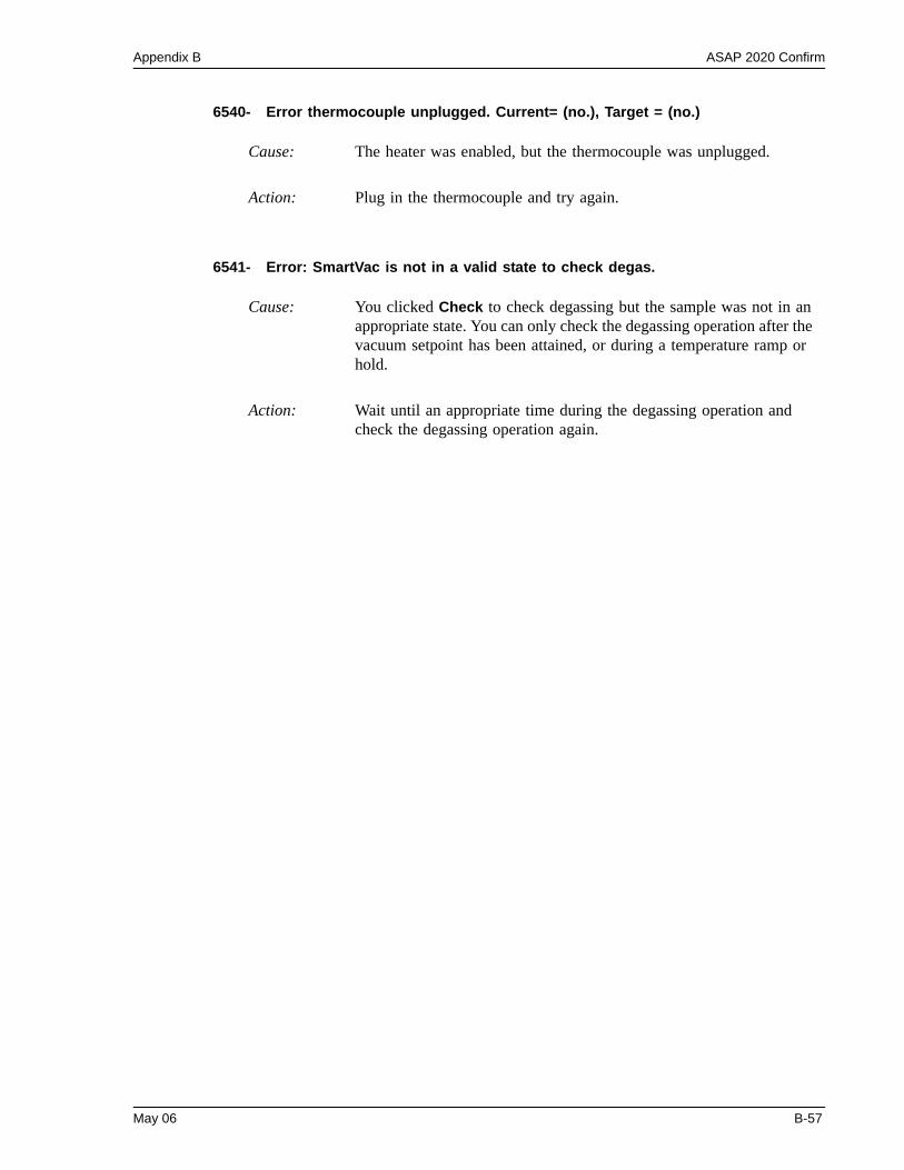
Appendix B ASAP 2020 Confirm
6540- Error thermocouple unplugged. Current= (no.), Target = (no.)
6541- Error: SmartVac is not in a valid state to check degas.
Cause: The heater was enabled, but the thermocouple was unplugged.
Action: Plug in the thermocouple and try again.
Cause: You clicked Check to check degassing but the sample was not in an appropriate state. You can only check the degassing operation after the vacuum setpoint has been attained, or during a temperature ramp or hold.
Action: Wait until an appropriate time during the degassing operation and check the degassing operation again.
May 06 B-57

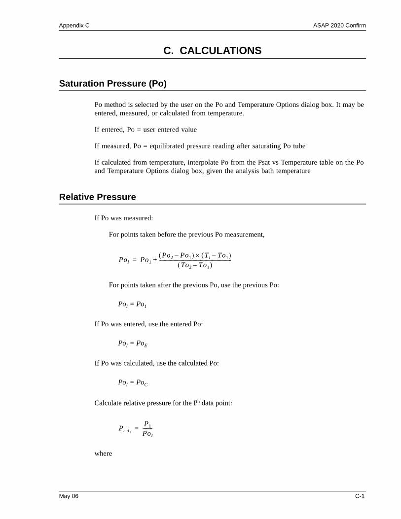
Appendix C ASAP 2020 Confirm
C. CALCULATIONS
Saturation Pressure (Po)
Po method is selected by the user on the Po and Temperature Options dialog box. It may be entered, measured, or calculated from temperature.
If entered, Po = user entered value
If measured, Po = equilibrated pressure reading after saturating Po tube
If calculated from temperature, interpolate Po from the Psat vs Temperature table on the Po and Temperature Options dialog box, given the analysis bath temperature
Relative Pressure
If Po was measured:
For points taken before the previous Po measurement,
For points taken after the previous Po, use the previous Po:
PoI = Po1
If Po was entered, use the entered Po:
PoI = PoE
If Po was calculated, use the calculated Po:
PoI = PoC
Calculate relative pressure for the Ith data point:
where
PoI Po1Po2 Po1–( ) TI To1–( )×
To2 To1–( )------------------------------------------------------------+=
Prel1
P1
PoI--------=
May 06 C-1
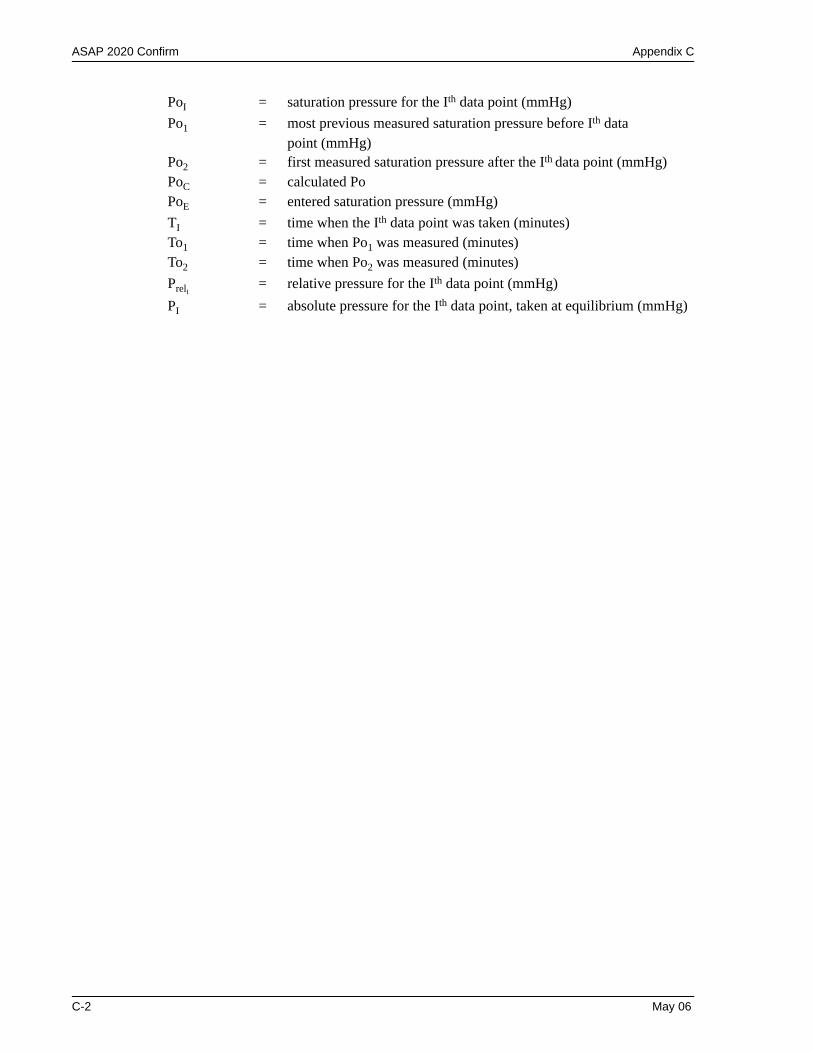
ASAP 2020 Confirm Appendix C
PoI = saturation pressure for the Ith data point (mmHg)Po1 = most previous measured saturation pressure before Ith data
point (mmHg)Po2 = first measured saturation pressure after the Ith data point (mmHg)PoC = calculated PoPoE = entered saturation pressure (mmHg)TI = time when the Ith data point was taken (minutes)To1 = time when Po1 was measured (minutes)To2 = time when Po2 was measured (minutes)PrelI
= relative pressure for the Ith data point (mmHg)PI = absolute pressure for the Ith data point, taken at equilibrium (mmHg)
C-2 May 06
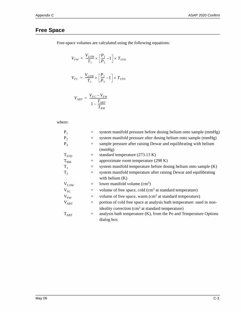
Appendix C ASAP 2020 Confirm
Free Space
Free-space volumes are calculated using the following equations:
where:
P1 = system manifold pressure before dosing helium onto sample (mmHg)P2 = system manifold pressure after dosing helium onto sample (mmHg)P3 = sample pressure after raising Dewar and equilibrating with helium
(mmHg)TSTD = standard temperature (273.13 K)TRM = approximate room temperature (298 K)T1 = system manifold temperature before dosing helium onto sample (K)T2 = system manifold temperature after raising Dewar and equilibrating
with helium (K)VLOW = lower manifold volume (cm3)VFC = volume of free space, cold (cm3 at standard temperature)VFW = volume of free space, warm (cm3 at standard temperature)VABT = portion of cold free space at analysis bath temperature: used in non-
ideality correction (cm3 at standard temperature)TABT = analysis bath temperature (K), from the Po and Temperature Options
dialog box
VFWVLOW
T1------------ P1
P2----- 1–× TSTD×=
VFCVLOW
T2------------ P1
P3----- 1–× TSTD×=
VABTVFC VFW–
1 TABT
TRM----------–
------------------------=
May 06 C-3
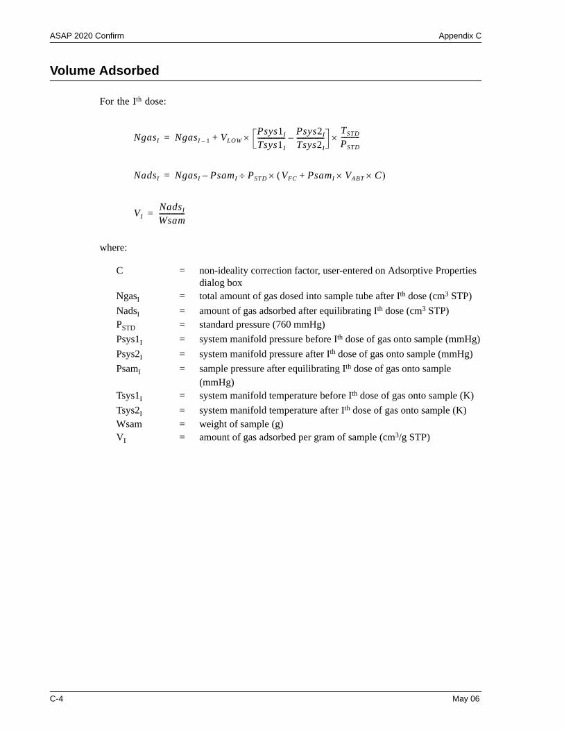
ASAP 2020 Confirm Appendix C
Volume Adsorbed
For the Ith dose:
where:
C = non-ideality correction factor, user-entered on Adsorptive Properties dialog box
NgasI = total amount of gas dosed into sample tube after Ith dose (cm3 STP)NadsI = amount of gas adsorbed after equilibrating Ith dose (cm3 STP)PSTD = standard pressure (760 mmHg)Psys1I = system manifold pressure before Ith dose of gas onto sample (mmHg)Psys2I = system manifold pressure after Ith dose of gas onto sample (mmHg)PsamI = sample pressure after equilibrating Ith dose of gas onto sample
(mmHg)Tsys1I = system manifold temperature before Ith dose of gas onto sample (K)Tsys2I = system manifold temperature after Ith dose of gas onto sample (K)Wsam = weight of sample (g) VI = amount of gas adsorbed per gram of sample (cm3/g STP)
NgasI NgasI 1– VLOWPsys1I
Tsys1I---------------- Psys2I
Tsys2I----------------–×
TSTD
PSTD-----------×+=
NadsI NgasI PsamI PSTD VFC PsamI VABT C××+( )×÷–=
VINadsI
Wsam---------------=
C-4 May 06
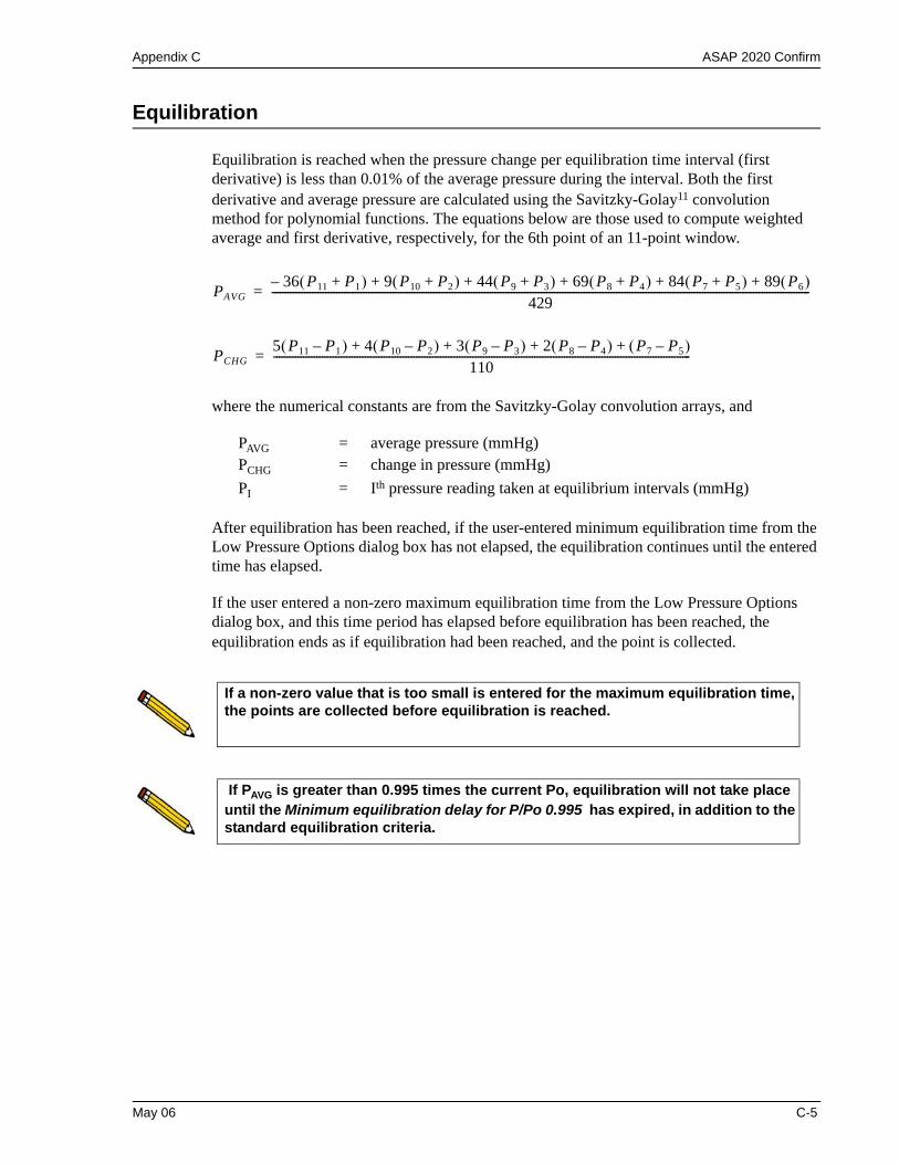
Appendix C ASAP 2020 Confirm
Equilibration
Equilibration is reached when the pressure change per equilibration time interval (first derivative) is less than 0.01% of the average pressure during the interval. Both the first derivative and average pressure are calculated using the Savitzky-Golay11 convolution method for polynomial functions. The equations below are those used to compute weighted average and first derivative, respectively, for the 6th point of an 11-point window.
where the numerical constants are from the Savitzky-Golay convolution arrays, and
PAVG = average pressure (mmHg)PCHG = change in pressure (mmHg)PI = Ith pressure reading taken at equilibrium intervals (mmHg)
After equilibration has been reached, if the user-entered minimum equilibration time from the Low Pressure Options dialog box has not elapsed, the equilibration continues until the entered time has elapsed.
If the user entered a non-zero maximum equilibration time from the Low Pressure Options dialog box, and this time period has elapsed before equilibration has been reached, the equilibration ends as if equilibration had been reached, and the point is collected.
PAVG36 P11 P1+( )– 9 P10 P2+( ) 44 P9 P3+( ) 69 P8 P4+( ) 84 P7 P5+( ) 89 P6( )+ + + + +
429--------------------------------------------------------------------------------------------------------------------------------------------------------------------------------------------------------=
PCHG5 P11 P1–( ) 4 P10 P2–( ) 3 P9 P3–( ) 2 P8 P4–( ) P7 P5–( )+ + + +
110-----------------------------------------------------------------------------------------------------------------------------------------------------------=
If a non-zero value that is too small is entered for the maximum equilibration time, the points are collected before equilibration is reached.
If PAVG is greater than 0.995 times the current Po, equilibration will not take place until the Minimum equilibration delay for P/Po 0.995 has expired, in addition to the standard equilibration criteria.
May 06 C-5
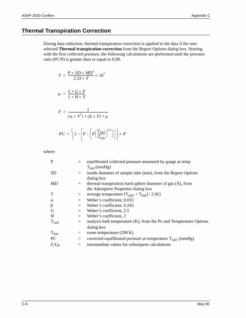
ASAP 2020 Confirm Appendix C
Thermal Transpiration Correction
During data reduction, thermal transpiration correction is applied to the data if the user selected Thermal transpiration correction from the Report Options dialog box. Starting with the first collected pressure, the following calculations are performed until the pressure ratio (PC/P) is greater than or equal to 0.99.
where:
P = equilibrated collected pressure measured by gauge at temp TRM (mmHg)
SD = inside diameter of sample tube (mm), from the Report Optionsdialog box
MD = thermal transpiration hard sphere diameter of gas (Å), from the Adsorptive Properties dialog box
T = average temperature [TABT + TRM] / 2 (K)α = Weber’s coefficient, 0.033β = Weber’s coefficient, 0.245G = Weber’s coefficient, 2.5H = Weber’s coefficient, 2 TABT = analysis bath temperature (K), from the Po and Temperature Options
dialog boxTRM = room temperature (298 K) PC = corrected equilibrated pressure at temperature TABT (mmHg)F,Y,µ = intermediate values for subsequent calculations
Y P SD MD2××2.33 T×
----------------------------------- 103×=
µ 1 G Y×+1 H Y×+-----------------------=
F 1α Y2×( ) β Y×( ) µ+ +
------------------------------------------------------=
PC 1 F FTABT
TRM----------⎝ ⎠
⎛ ⎞0.5
⎠⎞
⎭⎬⎫
P×⎝⎜⎛
––⎩⎨⎧
=
C-6 May 06
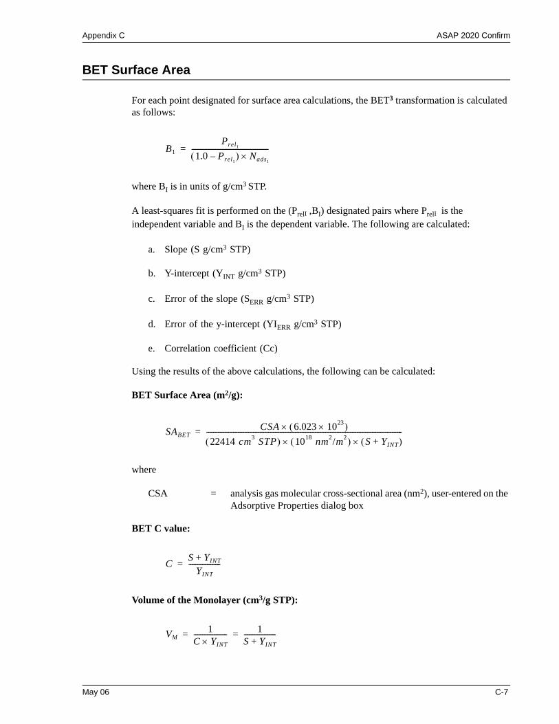
Appendix C ASAP 2020 Confirm
BET Surface Area
For each point designated for surface area calculations, the BET3 transformation is calculated as follows:
where BI is in units of g/cm3 STP.
A least-squares fit is performed on the (PrelI ,BI) designated pairs where PrelI is the independent variable and BI is the dependent variable. The following are calculated:
a. Slope (S g/cm3 STP)
b. Y-intercept (YINT g/cm3 STP)
c. Error of the slope (SERR g/cm3 STP)
d. Error of the y-intercept (YIERR g/cm3 STP)
e. Correlation coefficient (Cc)
Using the results of the above calculations, the following can be calculated:
BET Surface Area (m2/g):
where
CSA = analysis gas molecular cross-sectional area (nm2), user-entered on the Adsorptive Properties dialog box
BET C value:
Volume of the Monolayer (cm3/g STP):
B1Prel1
1.0 Prel1–( ) Nads1
×----------------------------------------------=
SABETCSA 6.023 1023×( )×
22414 cm3 STP( ) 1018 nm2/m2( ) S YINT+( )××---------------------------------------------------------------------------------------------------------------------=
C S YINT+YINT
-------------------=
VM1
C YINT×-------------------- 1
S YINT+-------------------= =
May 06 C-7

ASAP 2020 Confirm Appendix C
Error of the BET Surface Area (m2/g):
BETERRSABET SERR 2 YIERR 2+( )
0.5×
YINT S+---------------------------------------------------------------------=
C-8 May 06
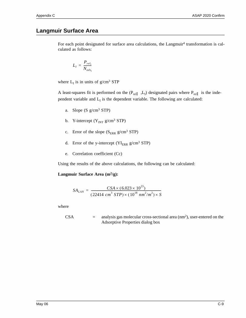
Appendix C ASAP 2020 Confirm
Langmuir Surface Area
For each point designated for surface area calculations, the Langmuir4 transformation is cal-culated as follows:
where LI is in units of g/cm3 STP
A least-squares fit is performed on the (PrelI ,LI) designated pairs where PrelI is the inde-pendent variable and LI is the dependent variable. The following are calculated:
a. Slope (S g/cm3 STP)
b. Y-intercept (YINT g/cm3 STP)
c. Error of the slope (SERR g/cm3 STP)
d. Error of the y-intercept (YIERR g/cm3 STP)
e. Correlation coefficient (Cc)
Using the results of the above calculations, the following can be calculated:
Langmuir Surface Area (m2/g):
where
CSA = analysis gas molecular cross-sectional area (nm2), user-entered on the Adsorptive Properties dialog box
LIPrelI
NadsI
-----------=
SALANCSA 6.023 1023×( )×
22414 cm3 STP( ) 1018 nm2/m2( ) S××-----------------------------------------------------------------------------------------------=
May 06 C-9
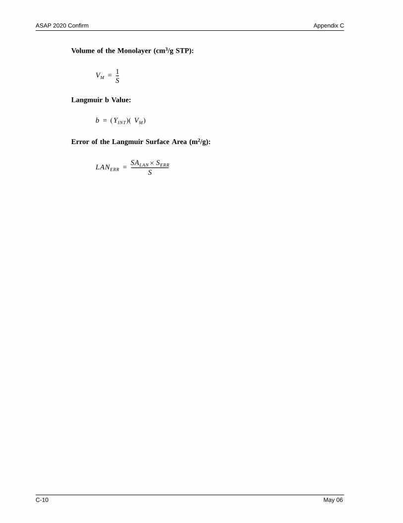
ASAP 2020 Confirm Appendix C
Volume of the Monolayer (cm3/g STP):
Langmuir b Value:
Error of the Langmuir Surface Area (m2/g):
VM1S---=
b YINT( ) VM( )=
LANERRSALAN SERR×
S-------------------------------=
C-10 May 06
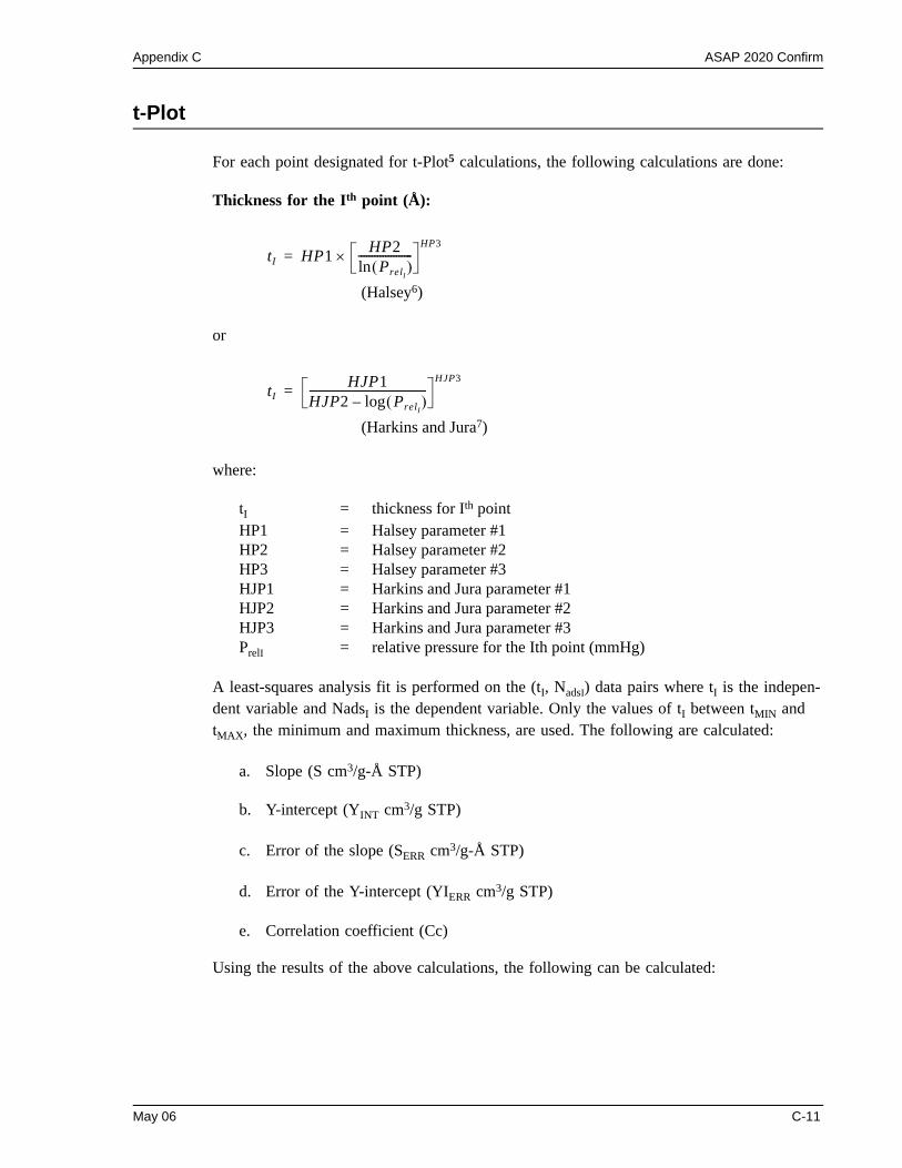
Appendix C ASAP 2020 Confirm
t-Plot
For each point designated for t-Plot5 calculations, the following calculations are done:
Thickness for the Ith point (Å):
(Halsey6)
or
(Harkins and Jura7)
where:
tI = thickness for Ith point HP1 = Halsey parameter #1HP2 = Halsey parameter #2HP3 = Halsey parameter #3HJP1 = Harkins and Jura parameter #1HJP2 = Harkins and Jura parameter #2HJP3 = Harkins and Jura parameter #3PrelI = relative pressure for the Ith point (mmHg)
A least-squares analysis fit is performed on the (tI, NadsI) data pairs where tI is the indepen-dent variable and NadsI is the dependent variable. Only the values of tI between tMIN and tMAX, the minimum and maximum thickness, are used. The following are calculated:
a. Slope (S cm3/g-Å STP)
b. Y-intercept (YINT cm3/g STP)
c. Error of the slope (SERR cm3/g-Å STP)
d. Error of the Y-intercept (YIERR cm3/g STP)
e. Correlation coefficient (Cc)
Using the results of the above calculations, the following can be calculated:
tI HP1 HP2PrelI
( )ln--------------------×
HP3=
tIHJP1
HJP2 PrelI( )log–
-------------------------------------------HJP3
=
May 06 C-11
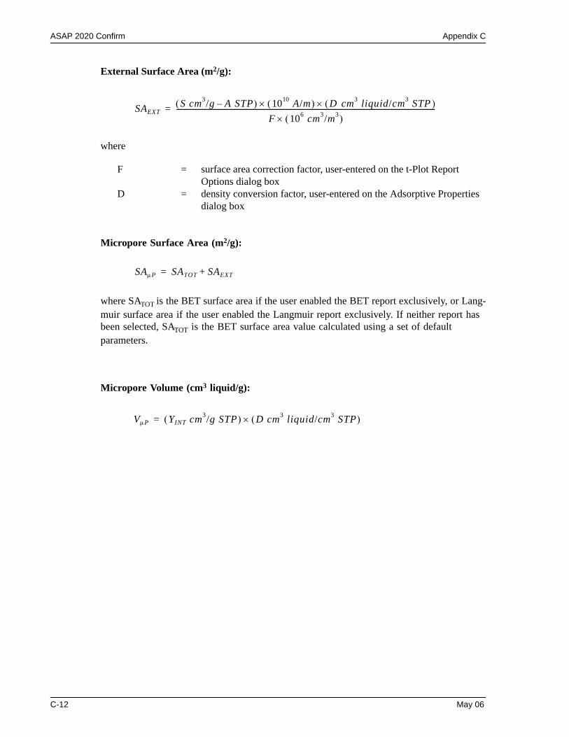
ASAP 2020 Confirm Appendix C
External Surface Area (m2/g):
where
F = surface area correction factor, user-entered on the t-Plot Report Options dialog box
D = density conversion factor, user-entered on the Adsorptive Properties dialog box
Micropore Surface Area (m2/g):
where SATOT is the BET surface area if the user enabled the BET report exclusively, or Lang-muir surface area if the user enabled the Langmuir report exclusively. If neither report has been selected, SATOT is the BET surface area value calculated using a set of default parameters.
Micropore Volume (cm3 liquid/g):
SAEXTS cm3/g A STP–( ) 1010 A/m( ) D( cm3 liquid/cm3 STP )××
F 106 cm3/m3( )×--------------------------------------------------------------------------------------------------------------------------------------------------------=
SAµP SATOT SAEXT+=
VµP YINT cm3/g STP( ) D cm3 liquid/cm3 STP( )×=
C-12 May 06
Appendix C ASAP 2020 Confirm
BJH Pore Volume and Area Distribution
For adsorption data, the relative pressure and volume adsorbed data point pairs collected dur-ing an analysis must be arranged in reverse order from which the points were collected during analysis. All calculations are performed based on a desorption model, regardless of whether adsorption or desorption data are being used.
The data used in these calculations must be in order of strictly decreasing numerical value. Points which do not meet this criterion are omitted. The remaining data set is composed of relative pressure (Pr), volume adsorbed (Va) pairs from (Pr1, Va1) to (PrN, VaN) where (PrN = 0, VaN = 0) is assumed as a final point. Each data pair represents an interval boundary (or des-orption step boundary) for intervals i=1 to i=N-1 where N = total number of (Pr, Va) pairs.
Generally, the desorption branch of an isotherm is used to relate the amount of adsorbate lost in a desorption step to the average size of pores emptied in the step. A pore loses its con-densed liquid adsorbate, known as the core of the pore, at a particular relative pressure related to the core radius by the Kelvin8 equation. After the core has evaporated, a layer of adsorbate remains on the wall of the pore. The thickness of this layer is calculated for a particular rel-ative pressure from the thickness equation. This layer becomes thinner with successive decreases in pressure, so that the measured quantity of gas desorbed in a step is composed of a quantity equivalent to the liquid cores evaporated in that step plus the quantity desorbed from the pore walls of pores whose cores have been evaporated in that and previous steps. Barrett, Joyner, and Halenda9 developed the method (known as the BJH method) which incor-porates these ideas. The algorithm used on the ASAP 2020 is an implementation of the BJH method.
Explanation of Terms
A pore filled with condensed liquid nitrogen has three zones:
a. The core - evaporates all at once when the critical pressure for that radius is reached; the relationship between the core radius and the critical pressure is defined by the Kelvin equation.
b. The adsorbed layer - composed of adsorbed gas that is stripped off a bit at a time with each pressure step; the relationship between the thickness of the layer and the relative pressure is defined by the thickness equation.
May 06 C-13
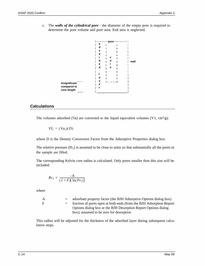
ASAP 2020 Confirm Appendix C
c. The walls of the cylindrical pore - the diameter of the empty pore is required to determine the pore volume and pore area. End area is neglected.
Calculations
The volumes adsorbed (Va) are converted to the liquid equivalent volumes (V1, cm3/g):
where D is the Density Conversion Factor from the Adsorptive Properties dialog box.
The relative pressure (Pr1) is assumed to be close to unity so that substantially all the pores in the sample are filled.
The corresponding Kelvin core radius is calculated. Only pores smaller than this size will be included:
where
A = adsorbate property factor (the BJH Adsorptive Options dialog box)F = fraction of pores open at both ends (from the BJH Adsorption Report
Options dialog box or the BJH Desorption Report Options dialog box); assumed to be zero for desorption
This radius will be adjusted for the thickness of the adsorbed layer during subsequent calcu-lation steps.
adsorbed
layer
wallcore
Insignificant compared to core length
pore
VII VaI( ) D( )=
RcIA–
1 F+( ) PrI( )ln[ ]-----------------------------------------=
C-14 May 06
Appendix C ASAP 2020 Confirm
The thickness of the remaining adsorbed layer at this relative pressure is calculated:
where
HP1, HP2, and HP3 are Halsey Parameters 1, 2, and 3 (respectively) from the Halsey Thick-ness Equation dialog box.
These calculations illustrate the use of the Halsey thickness equation. If the Harkins/Jura equation was selected, substitute the following wherever the thickness equation appears:
where
HJ1, HJ2, and HJ3 are Harkins-Jura Parameters 1, 2, and 3 (respectively) from the Harkins-Jura Thickness Equation dialog box.
The following calculations (a-c) are made for each relative pressure interval based on the increment of volume desorbed during that interval. The variable I refers to the interval num-ber, that is I=1 for the first interval from Pr1 to Pr2, and so on. J refers to each previous interval during which new pores were found. K refers to the total number of intervals in which new pores have been found. K is also the number of lines reported on the BJH table for collected data.
a. The thickness of the adsorbed layer at the end of the interval is calculated as follows:
(For the last pressure interval from the lowest PrI to zero relative pressure, TwI+1 = 0.)
For the first pressure interval, there are no previously opened pores so the volume desorbed from walls of previously opened pores is zero (Vd1 = 0), and the remainder of Step a is skipped.
The change in thickness of the wall layer due to desorption from preivously opened pores is calculated:
Tw1 HP1 HP2Pr1( )ln
------------------HP3
=
Tw1HJ1
HJ2 Pr1( )log–--------------------------------------
HJ3=
TwI 1+ HP1 HP2PrI 1+( )ln
------------------------HP3
=
∆Tw Tw1 TwI 1+–=
May 06 C-15
ASAP 2020 Confirm Appendix C
The annular cross-sectional area of the wall layer desorbed is calculated for all pre-viously opened pores:
The total volume of gas desorbed from walls of previously opened pores is calculated:
for all previously opened pores
where LPJ = length of previously opened pores as calculated in Step b(2).
b. The physical processes occurring for this pressure interval are determined as follows:
(1) If VdI is greater than the current increment of volume desorbed (VlI - VlI+1), desorption from walls only is occurring. Total surface of walls exposed thus far (cm2/g) is calculated as follows:
for all previously opened pores
where
DavgJ = weighted average pore diameter calculated below in Step b(2).
A new layer thickness (∆Tw) that will not overcompensate for the actual volume desorbed in this interval is calculated:
Since no cores are evaporated in this pressure interval, no new pores are revealed. Thus no ending Kelvin radius and average pore diameter are calculated for this interval. Note that this means the report may have fewer tabulated intervals on the collected data report than experimental pressure intervals.
(2) If VdI is less than the volume increment desorbed during this interval, the remaining volume is due to new pores with core evaporation taking place in this interval. K, the number of intervals with new pores exposed, is increased by 1. (For the interval from the lowest to zero relative pressure, no new pore volume is calculated and the rest of Step b is skipped.)
The volume desorbed from newly opened pores in this interval is calculated as follows:
CSAJ π Rcj ∆Tw+( )2 Rcj 2–[ ] 10 16– cm2/A2( )=
VdI LpJ( ) CSAaJ( )∑=
SAW π LPJ( ) DavgJ( ) 10 8– cm/A( )∑=
∆Tw V1I V1I 1+–( ) 108 A/cm( )SAwI
--------------------------------------------------------------=
VcI VII VII 1+–( ) VdI–=
C-16 May 06
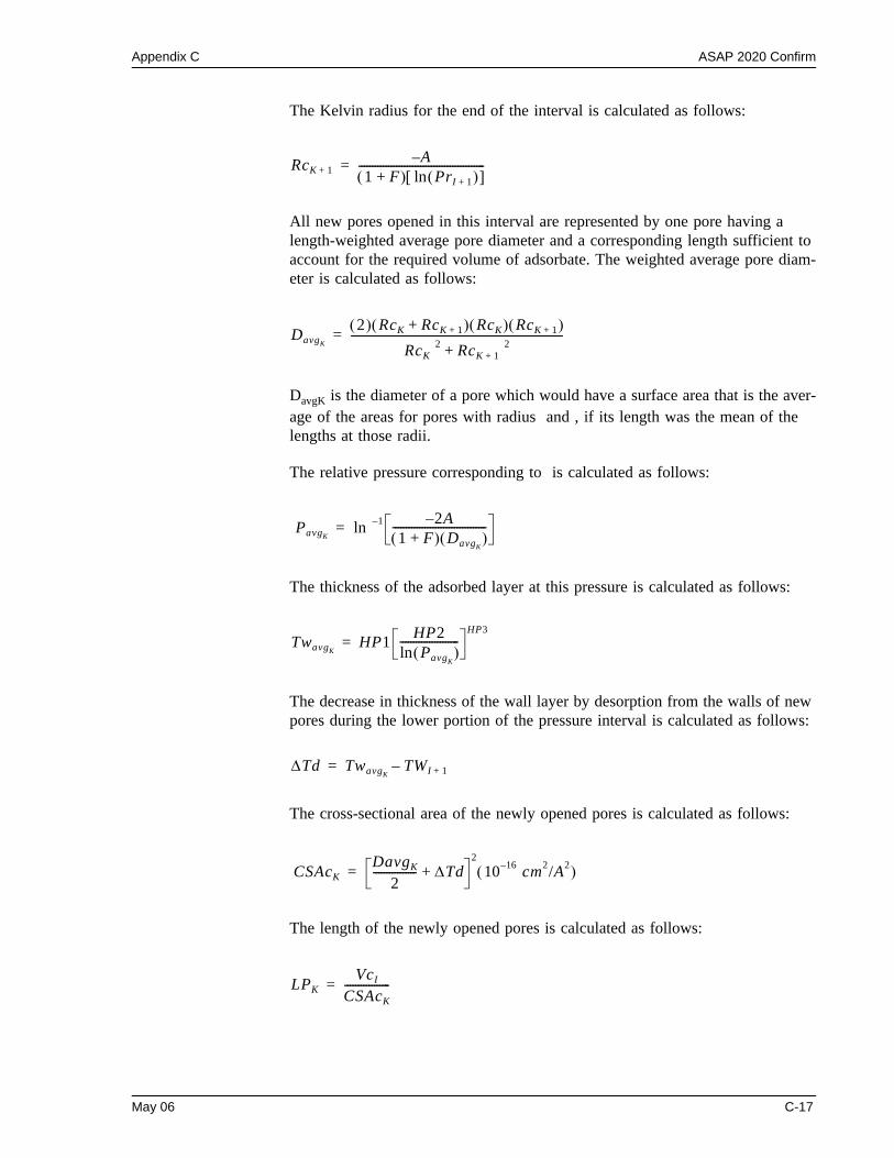
Appendix C ASAP 2020 Confirm
The Kelvin radius for the end of the interval is calculated as follows:
All new pores opened in this interval are represented by one pore having a length-weighted average pore diameter and a corresponding length sufficient to account for the required volume of adsorbate. The weighted average pore diam-eter is calculated as follows:
DavgK is the diameter of a pore which would have a surface area that is the aver-age of the areas for pores with radius and , if its length was the mean of the lengths at those radii.
The relative pressure corresponding to is calculated as follows:
The thickness of the adsorbed layer at this pressure is calculated as follows:
The decrease in thickness of the wall layer by desorption from the walls of new pores during the lower portion of the pressure interval is calculated as follows:
The cross-sectional area of the newly opened pores is calculated as follows:
The length of the newly opened pores is calculated as follows:
RcK 1+A–
1 F+( ) PrI 1+( )ln[ ]-----------------------------------------------=
DavgK
2( ) RcK RcK 1++( ) RcK( ) RcK 1+( )
RcK 2 RcK 1+ 2+-------------------------------------------------------------------------------=
PavgK 1– 2A–
1 F+( ) DavgK( )
-----------------------------------ln=
TwavgKHP1 HP2
PavgK( )ln
----------------------HP3
=
∆Td TwavgKTWI 1+–=
CSAcKDavgK
2---------------- ∆Td+
210 16– cm2/A2( )=
LPKVcI
CSAcK-----------------=
May 06 C-17
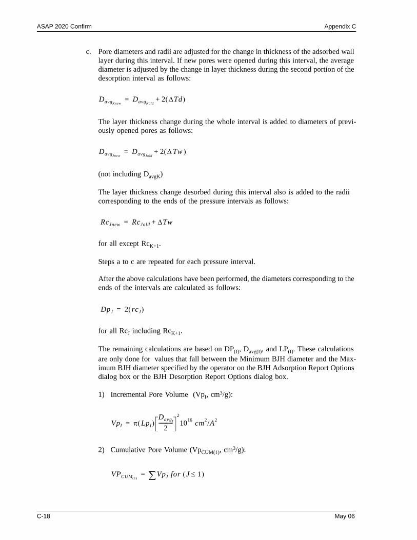
ASAP 2020 Confirm Appendix C
c. Pore diameters and radii are adjusted for the change in thickness of the adsorbed wall layer during this interval. If new pores were opened during this interval, the average diameter is adjusted by the change in layer thickness during the second portion of the desorption interval as follows:
The layer thickness change during the whole interval is added to diameters of previ-ously opened pores as follows:
(not including DavgK)
The layer thickness change desorbed during this interval also is added to the radii corresponding to the ends of the pressure intervals as follows:
for all except RcK+1.
Steps a to c are repeated for each pressure interval.
After the above calculations have been performed, the diameters corresponding to the ends of the intervals are calculated as follows:
for all RcJ including RcK+1.
The remaining calculations are based on DP(I), Davg(I), and LP(I). These calculations are only done for values that fall between the Minimum BJH diameter and the Max-imum BJH diameter specified by the operator on the BJH Adsorption Report Options dialog box or the BJH Desorption Report Options dialog box.
1) Incremental Pore Volume (VpI, cm3/g):
2) Cumulative Pore Volume (VpCUM(1), cm3/g):
DavgKnewDavgKold
2 ∆Td( )+=
DavgJnewDavgJold
2 ∆( Tw )+=
RcJnew RcJold ∆Tw+=
DpJ 2 rcJ( )=
VpI π LpI( )DavgI
2-----------
2
1016 cm2/A2=
VPCUM 1( )VpJ for J 1≤( )∑=
C-18 May 06
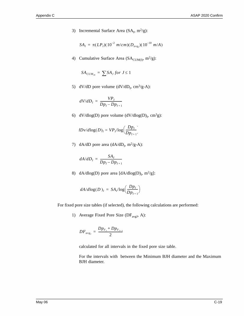
Appendix C ASAP 2020 Confirm
3) Incremental Surface Area (SAI, m2/g):
4) Cumulative Surface Area (SACUM(I), m2/g):
5) dV/dD pore volume (dV/dDI, cm3/g-A):
6) dV/dlog(D) pore volume (dV/dlog(D)I, cm3g):
7) dA/dD pore area (dA/dDI, m2/g-A):
8) dA/dlog(D) pore area [dA/dlog(D)I, m2/g]:
For fixed pore size tables (if selected), the following calculations are performed:
1) Average Fixed Pore Size (DFavgJ, A):
calculated for all intervals in the fixed pore size table.
For the intervals with between the Minimum BJH diameter and the Maximum BJH diameter.
SAI π LPI( ) 10 2– m/cm( ) DavgI( ) 10 10– m/A( )=
SACUM10SAJ for J 1≤∑=
dV/dDIVPI
DpI DpI 1+–------------------------------=
dDv/d D( )I VPI/DpI
DpI 1+---------------⎝ ⎠
⎛ ⎞log=log
dA/dDISAI
DpI DpI 1+–------------------------------=
dA/d D( )Ilog SAI/DpI
DpI 1+---------------⎝ ⎠
⎛ ⎞log=
DFavgJ
DpFJDpFJ 1+
+2
---------------------------------=
May 06 C-19
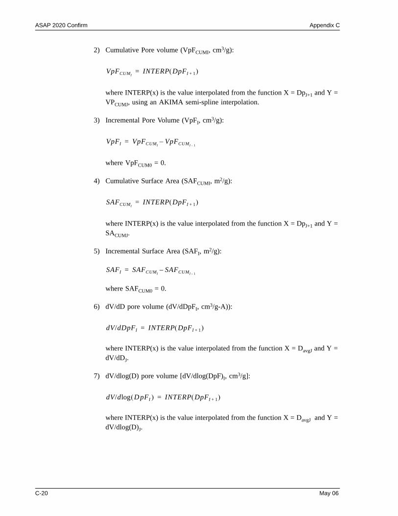
ASAP 2020 Confirm Appendix C
2) Cumulative Pore volume (VpFCUMI, cm3/g):
where INTERP(x) is the value interpolated from the function X = DpJ+1 and Y = VPCUMJ, using an AKIMA semi-spline interpolation.
3) Incremental Pore Volume (VpFI, cm3/g):
where VpFCUM0 = 0.
4) Cumulative Surface Area (SAFCUMI, m2/g):
where INTERP(x) is the value interpolated from the function X = DpJ+1 and Y = SACUMJ.
5) Incremental Surface Area (SAFI, m2/g):
where SAFCUM0 = 0.
6) dV/dD pore volume (dV/dDpFI, cm3/g-A)):
where INTERP(x) is the value interpolated from the function X = DavgJ and Y = dV/dDJ.
7) dV/dlog(D) pore volume [dV/dlog(DpF)I, cm3/g]:
where INTERP(x) is the value interpolated from the function X = DavgJ and Y = dV/dlog(D)J.
VpFCUMIINTERP DpFI 1+( )=
VpFI VpFCUMIVpFCUMI 1–
–=
SAFCUMIINTERP DpFI 1+( )=
SAFI SAFCUMISAFCUMI 1–
–=
dV/dDpFI INTERP DpFI 1+( )=
dV/d D( pFI )log INTERP DpFI 1+( )=
C-20 May 06
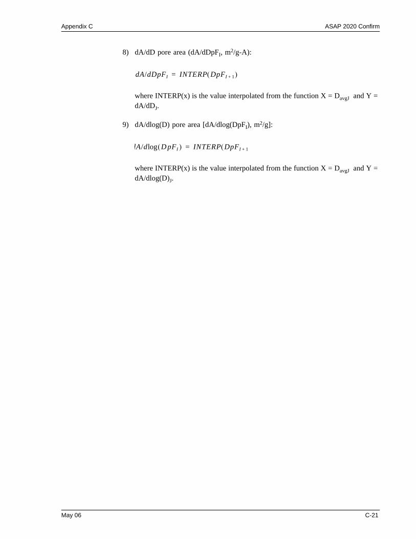
Appendix C ASAP 2020 Confirm
8) dA/dD pore area (dA/dDpFI, m2/g-A):
where INTERP(x) is the value interpolated from the function X = DavgJ and Y = dA/dDJ.
9) dA/dlog(D) pore area [dA/dlog(DpFI), m2/g]:
where INTERP(x) is the value interpolated from the function X = DavgJ and Y = dA/dlog(D)J.
dA/dDpFI INTERP DpFI 1+( )=
dA/d D( pFI )log INTERP DpFI 1+( )=
May 06 C-21
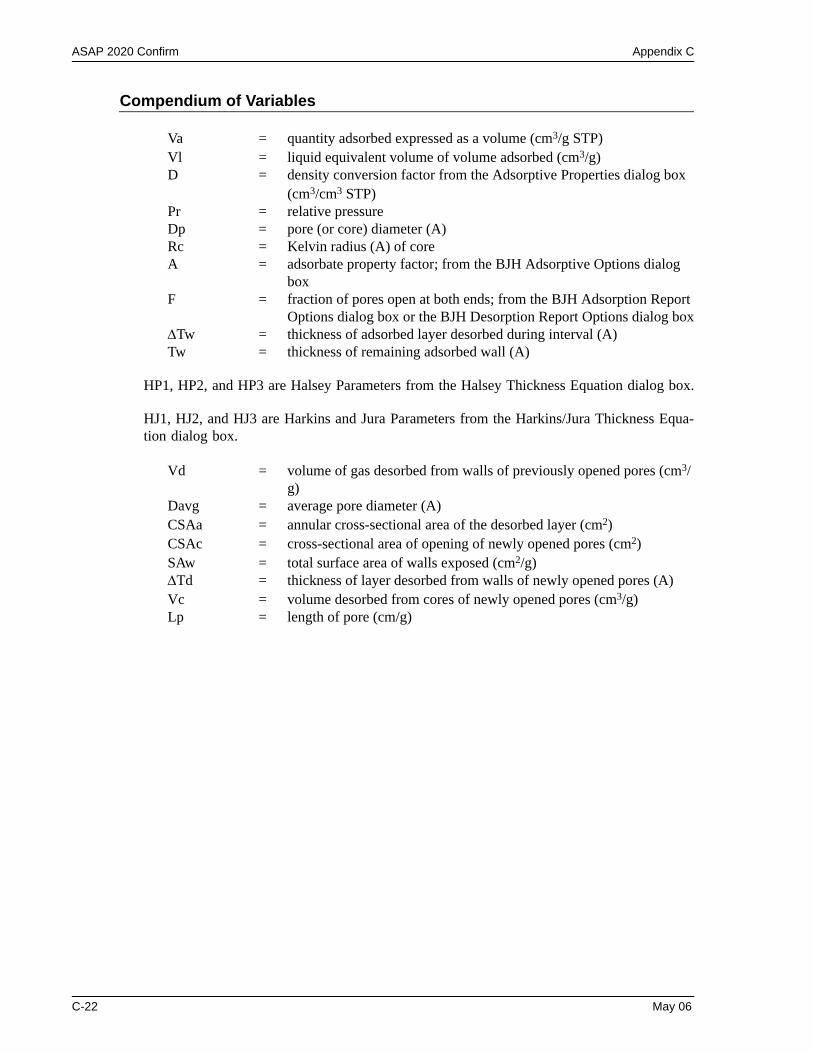
ASAP 2020 Confirm Appendix C
Compendium of Variables
Va = quantity adsorbed expressed as a volume (cm3/g STP)Vl = liquid equivalent volume of volume adsorbed (cm3/g)D = density conversion factor from the Adsorptive Properties dialog box
(cm3/cm3 STP)Pr = relative pressureDp = pore (or core) diameter (A)Rc = Kelvin radius (A) of coreA = adsorbate property factor; from the BJH Adsorptive Options dialog
boxF = fraction of pores open at both ends; from the BJH Adsorption Report
Options dialog box or the BJH Desorption Report Options dialog box∆Tw = thickness of adsorbed layer desorbed during interval (A)Tw = thickness of remaining adsorbed wall (A)
HP1, HP2, and HP3 are Halsey Parameters from the Halsey Thickness Equation dialog box.
HJ1, HJ2, and HJ3 are Harkins and Jura Parameters from the Harkins/Jura Thickness Equa-tion dialog box.
Vd = volume of gas desorbed from walls of previously opened pores (cm3/g)
Davg = average pore diameter (A)CSAa = annular cross-sectional area of the desorbed layer (cm2)CSAc = cross-sectional area of opening of newly opened pores (cm2)SAw = total surface area of walls exposed (cm2/g)∆Td = thickness of layer desorbed from walls of newly opened pores (A)Vc = volume desorbed from cores of newly opened pores (cm3/g)Lp = length of pore (cm/g)
C-22 May 06
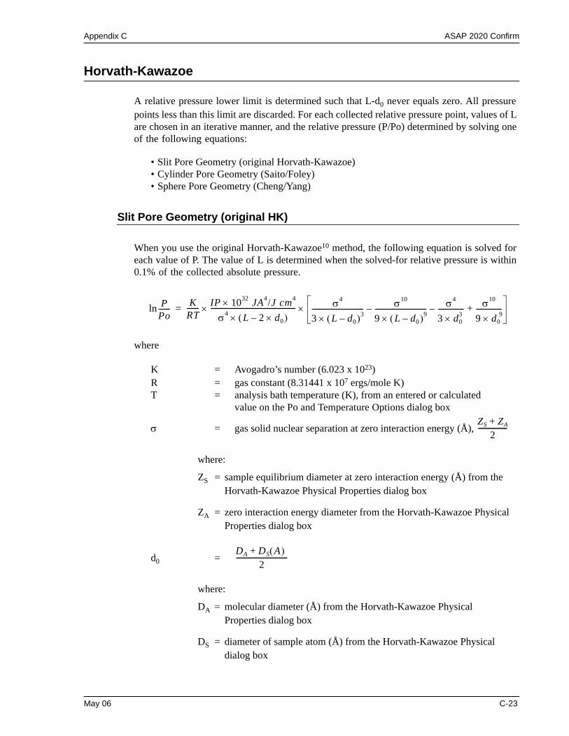
Appendix C ASAP 2020 Confirm
Horvath-Kawazoe
A relative pressure lower limit is determined such that L-d0 never equals zero. All pressure points less than this limit are discarded. For each collected relative pressure point, values of L are chosen in an iterative manner, and the relative pressure (P/Po) determined by solving one of the following equations:
• Slit Pore Geometry (original Horvath-Kawazoe)• Cylinder Pore Geometry (Saito/Foley)• Sphere Pore Geometry (Cheng/Yang)
Slit Pore Geometry (original HK)
When you use the original Horvath-Kawazoe10 method, the following equation is solved for each value of P. The value of L is determined when the solved-for relative pressure is within 0.1% of the collected absolute pressure.
where
K = Avogadro’s number (6.023 x 10²³)R = gas constant (8.31441 x 10⁷ ergs/mole K)T = analysis bath temperature (K), from an entered or calculated
value on the Po and Temperature Options dialog box
σ = gas solid nuclear separation at zero interaction energy (Å),
where:
ZS = sample equilibrium diameter at zero interaction energy (Å) from the Horvath-Kawazoe Physical Properties dialog box
ZA = zero interaction energy diameter from the Horvath-Kawazoe Physical Properties dialog box
d0 =
where:
DA = molecular diameter (Å) from the Horvath-Kawazoe PhysicalProperties dialog box
DS = diameter of sample atom (Å) from the Horvath-Kawazoe Physical dialog box
PPo-------ln K
RT------- IP 1032 JA4/J cm4×
σ4 L 2 d0×–( )×--------------------------------------------------× σ4
3 L d0–( )3×------------------------------ σ10
9 L d0–( )9×------------------------------– σ4
3 d0 3×
---------------– σ10
9 d0 9×
---------------+×=
ZS ZA+2
-----------------
DA DS A( ) +2
------------------------------
May 06 C-23
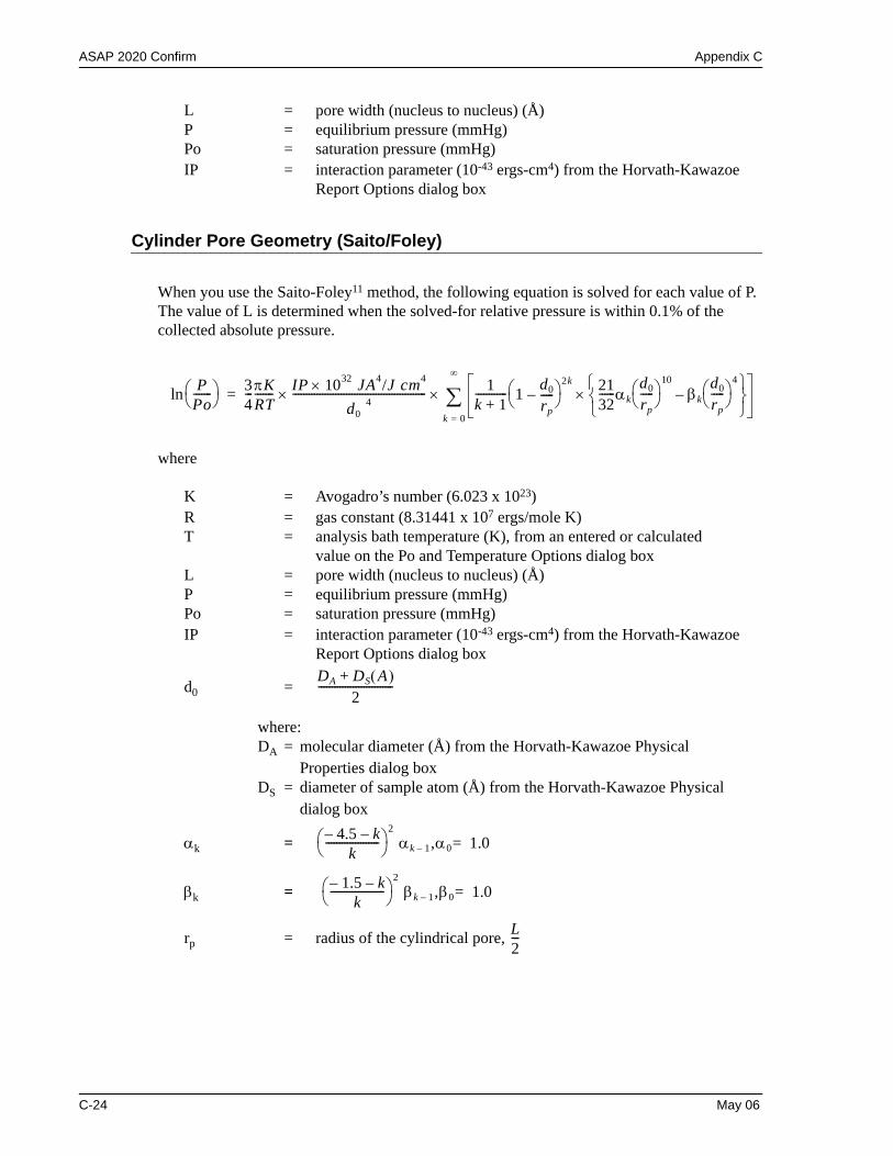
ASAP 2020 Confirm Appendix C
L = pore width (nucleus to nucleus) (Å)P = equilibrium pressure (mmHg)Po = saturation pressure (mmHg)IP = interaction parameter (10-43 ergs-cm4) from the Horvath-Kawazoe
Report Options dialog box
Cylinder Pore Geometry (Saito/Foley)
When you use the Saito-Foley11 method, the following equation is solved for each value of P. The value of L is determined when the solved-for relative pressure is within 0.1% of the collected absolute pressure.
where
K = Avogadro’s number (6.023 x 10²³)R = gas constant (8.31441 x 10⁷ ergs/mole K)T = analysis bath temperature (K), from an entered or calculated
value on the Po and Temperature Options dialog boxL = pore width (nucleus to nucleus) (Å)P = equilibrium pressure (mmHg)Po = saturation pressure (mmHg)IP = interaction parameter (10-43 ergs-cm4) from the Horvath-Kawazoe
Report Options dialog box
d0 =
where:DA = molecular diameter (Å) from the Horvath-Kawazoe Physical
Properties dialog box DS = diameter of sample atom (Å) from the Horvath-Kawazoe Physical
dialog box
αk =
βk =
rp = radius of the cylindrical pore,
PPo-------⎝ ⎠
⎛ ⎞ln 34---πK
RT------- IP 1032 JA4/J cm4×
d0 4--------------------------------------------------× 1
k 1+------------ 1 d0
rp-----–⎝ ⎠
⎛ ⎞ 2k 2132------αk
d0
rp-----⎝ ⎠
⎛ ⎞10
βkd0
rp-----⎝ ⎠
⎛ ⎞4
–⎩ ⎭⎨ ⎬⎧ ⎫
×k 0=
∞
∑×=
DA DS A( )+2
----------------------------
4.5– k–k
--------------------⎝ ⎠⎛ ⎞
2 αk 1– ,α0 1.0=
1.5– k–k
--------------------⎝ ⎠⎛ ⎞
2 βk 1– ,β0 1.0=
L2---
C-24 May 06
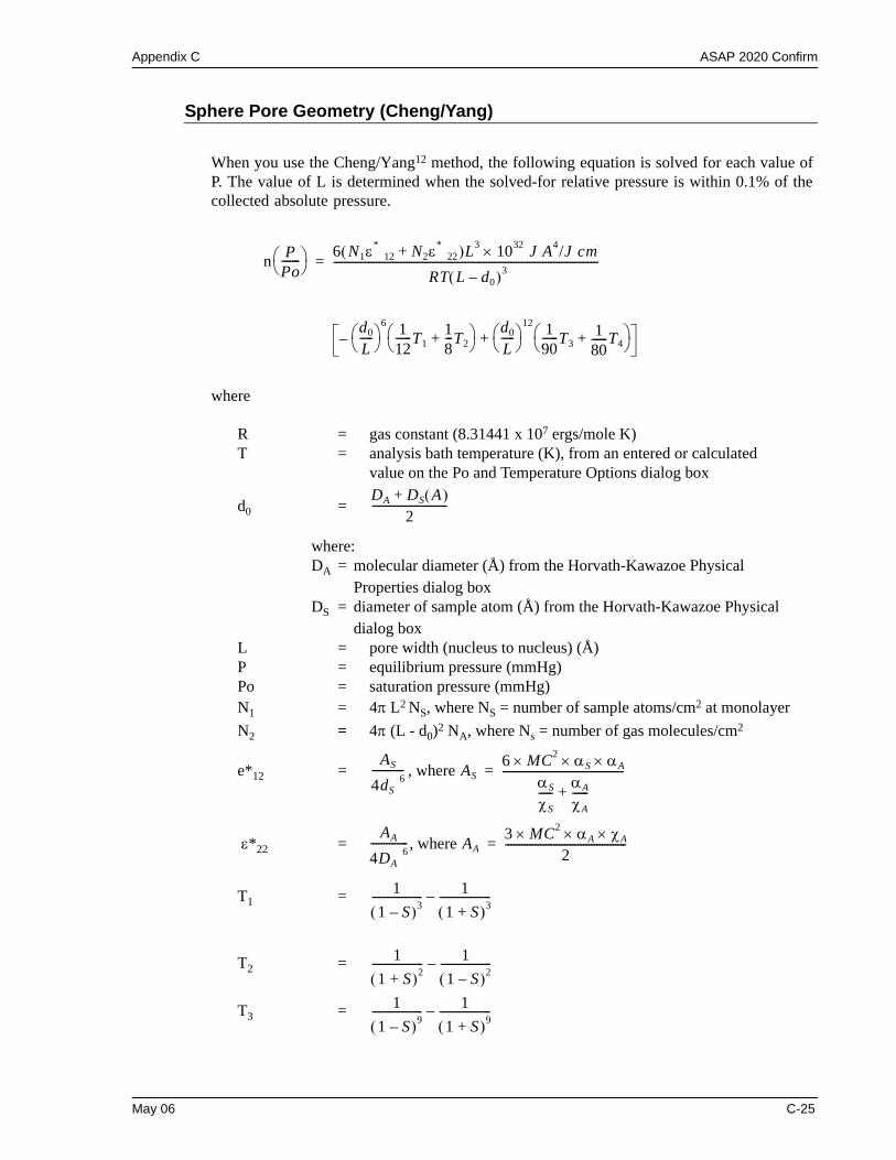
Appendix C ASAP 2020 Confirm
Sphere Pore Geometry (Cheng/Yang)
When you use the Cheng/Yang12 method, the following equation is solved for each value of P. The value of L is determined when the solved-for relative pressure is within 0.1% of the collected absolute pressure.
where
R = gas constant (8.31441 x 10⁷ ergs/mole K)T = analysis bath temperature (K), from an entered or calculated
value on the Po and Temperature Options dialog box
d0 =
where:DA = molecular diameter (Å) from the Horvath-Kawazoe Physical
Properties dialog box DS = diameter of sample atom (Å) from the Horvath-Kawazoe Physical
dialog box L = pore width (nucleus to nucleus) (Å)P = equilibrium pressure (mmHg)Po = saturation pressure (mmHg)N1 = 4π L2 NS, where NS = number of sample atoms/cm2 at monolayerN2 = 4π (L - d0)2 NA, where Ns = number of gas molecules/cm2
e*12 = , where
ε*22 = , where
T1 =
T2 =
T3 =
PPo-------⎝ ⎠
⎛ ⎞n 6 N1ε* 12 N2ε* 22+( )L3 1032 J A4/J cm4×
RT L d0–( )3----------------------------------------------------------------------------------------------------=
d0
L-----⎝ ⎠
⎛ ⎞6 1
12------T1
18---T2+⎝ ⎠
⎛ ⎞–d0
L-----⎝ ⎠
⎛ ⎞12 1
90------T3
180------+ T4⎝ ⎠
⎛ ⎞+
DA DS A( )+2
----------------------------
AS
4dS 6------------ AS
6 MC2 αS αA×××αS
χS----- αA
χA------+
---------------------------------------------=
AA
4DA 6-------------- AA
3 MC2 αA χA×××2
---------------------------------------------=
11 S–( )3
------------------- 11 S+( )3
-------------------–
11 S+( )2
------------------- 11 S–( )2
-------------------–
11 S–( )9
------------------- 11 S+( )9
-------------------–
May 06 C-25
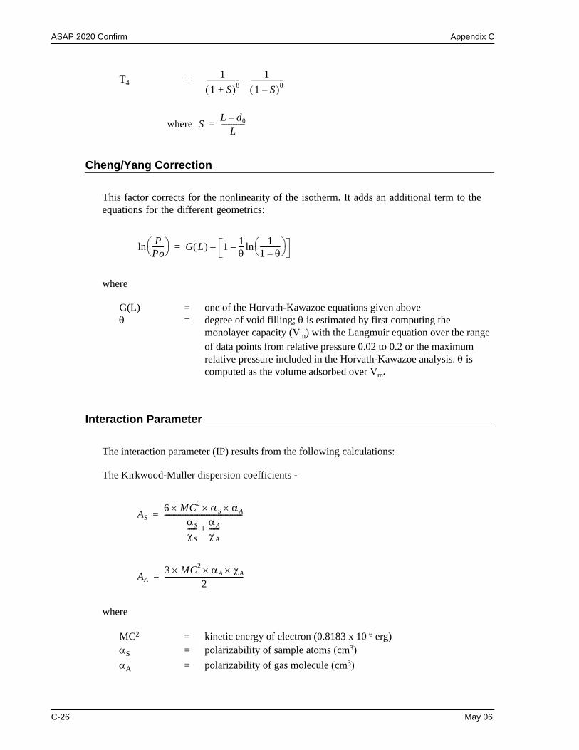
ASAP 2020 Confirm Appendix C
T4 =
where
Cheng/Yang Correction
This factor corrects for the nonlinearity of the isotherm. It adds an additional term to the equations for the different geometrics:
where
G(L) = one of the Horvath-Kawazoe equations given aboveθ = degree of void filling; θ is estimated by first computing the
monolayer capacity (Vm) with the Langmuir equation over the range of data points from relative pressure 0.02 to 0.2 or the maximum relative pressure included in the Horvath-Kawazoe analysis. θ is computed as the volume adsorbed over Vm.
Interaction Parameter
The interaction parameter (IP) results from the following calculations:
The Kirkwood-Muller dispersion coefficients -
where
MC2 = kinetic energy of electron (0.8183 x 10⁻⁶ erg)αS = polarizability of sample atoms (cm3)αA = polarizability of gas molecule (cm3)
11 S+( )8
------------------- 11 S–( )8
-------------------–
S L d0–L
--------------=
PPo-------⎝ ⎠
⎛ ⎞ln G L( ) 1 1θ--- 1
1 θ–------------⎝ ⎠
⎛ ⎞ln––=
AS6 MC2 αS αA×××
αS
χS----- αA
χA------+
---------------------------------------------=
AA3 MC2 αA χA×××
2---------------------------------------------=
C-26 May 06
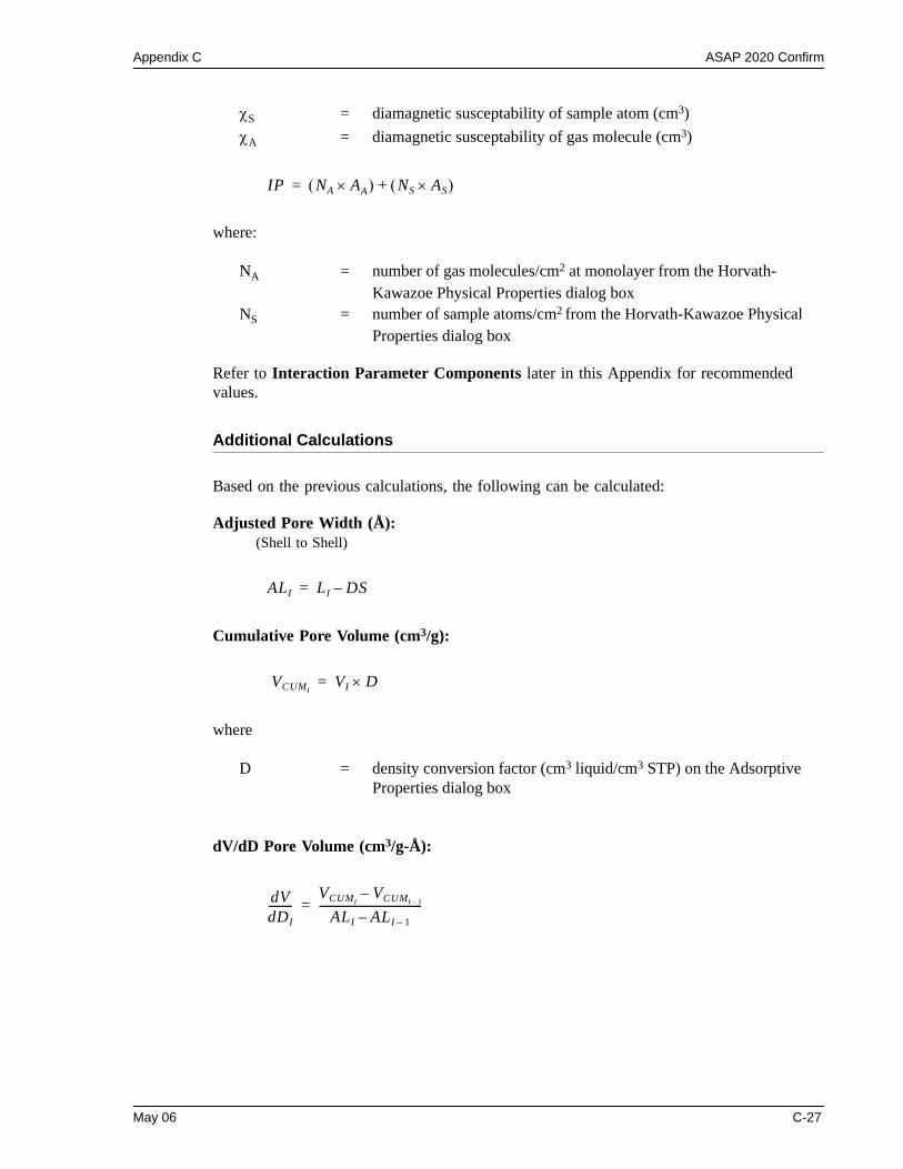
Appendix C ASAP 2020 Confirm
χS = diamagnetic susceptability of sample atom (cm3)χA = diamagnetic susceptability of gas molecule (cm3)
where:
NA = number of gas molecules/cm2 at monolayer from the Horvath-Kawazoe Physical Properties dialog box
NS = number of sample atoms/cm2 from the Horvath-Kawazoe Physical Properties dialog box
Refer to Interaction Parameter Components later in this Appendix for recommended values.
Additional Calculations
Based on the previous calculations, the following can be calculated:
Adjusted Pore Width (Å): (Shell to Shell)
Cumulative Pore Volume (cm3/g):
where
D = density conversion factor (cm3 liquid/cm3 STP) on the Adsorptive Properties dialog box
dV/dD Pore Volume (cm3/g-Å):
IP NA A× A( ) NS AS×( )+=
ALI LI DS–=
VCUMIVI D×=
dVdDI---------
VCUMIVCUMI 1–
–ALI ALI 1––
--------------------------------------=
May 06 C-27
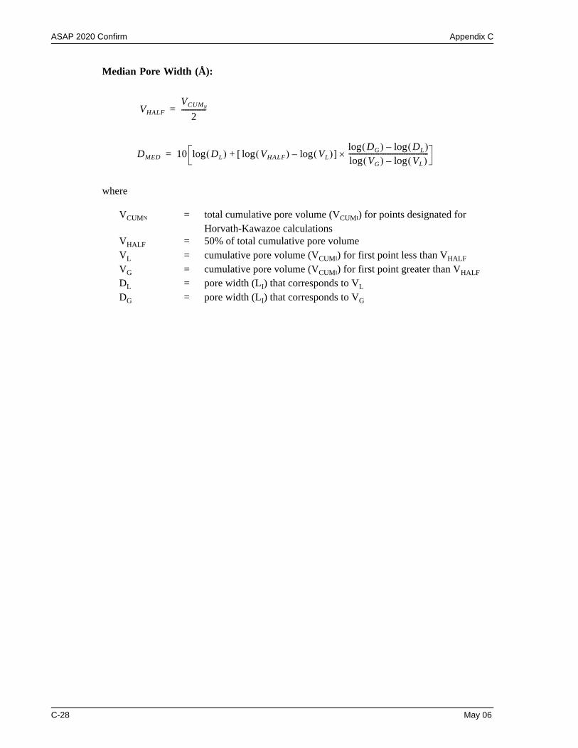
ASAP 2020 Confirm Appendix C
Median Pore Width (Å):
where
VCUMN = total cumulative pore volume (VCUMI) for points designated for Horvath-Kawazoe calculations
VHALF = 50% of total cumulative pore volume VL = cumulative pore volume (VCUMI) for first point less than VHALFVG = cumulative pore volume (VCUMI) for first point greater than VHALFDL = pore width (LI) that corresponds to VL DG = pore width (LI) that corresponds to VG
VHALFVCUMN
2--------------=
DMED 10 DL( )log VHALF( ) VL( )log–log[ ]DG( ) DL( )log–logVG( ) VL( )log–log
----------------------------------------------×+=
C-28 May 06
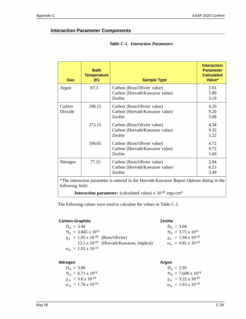
Appendix C ASAP 2020 Confirm
Interaction Parameter Components
Table C-1. Interaction Parameters
The following values were used to calculate the values in Table C-1.
Gas
Bath Temperature
(K) Sample Type
Interaction Parameter Calculated
Value*
Argon 87.3 Carbon (Ross/Olivier value)Carbon (Horvath/Kawazoe value)Zeolite
2.615.893.19
Carbon Dioxide
298.15 Carbon (Ross/Olivier value)Carbon (Horvath/Kawazoe value)Zeolite
4.209.205.08
273.15 Carbon (Ross/Olivier value)Carbon (Horvath/Kawazoe value)Zeolite
4.349.355.22
194.65 Carbon (Ross/Olivier value)Carbon (Horvath/Kawazoe value)Zeolite
4.729.725.60
Nitrogen 77.15 Carbon (Ross/Olivier value)Carbon (Horvath/Kawazoe value)Zeolite
2.846.533.49
*The interaction parameter is entered in the Horvath-Kawazoe Report Options dialog in the following field:
Interaction parameter: (calculated value) x 10-43 ergs-cm4
Carbon-Graphite ZeoliteDS = 3.40 DS = 3.04NS = 3.845 x 10¹⁵ NS = 3.75 x 10¹⁵
χS = 1.05 x 10⁻²⁹ (Ross/Olivier) χS = 1.94 x 10⁻²⁹
13.5 x 10⁻²⁹ (Horvath/Kawazoe, implicit) αS = 0.85 x 10⁻²⁴
αS = 1.02 x 10⁻²⁴
Nitrogen ArgonDA = 3.00 DA = 2.95ΝA = 6.71 x 10¹⁴ ΝA = 7.608 x 10¹⁴
χA = 3.6 x 10⁻²⁹ χA = 3.22 x 10⁻²⁹
αA = 1.76 x 10⁻²⁴ αA = 1.63 x 10⁻²⁴
May 06 C-29
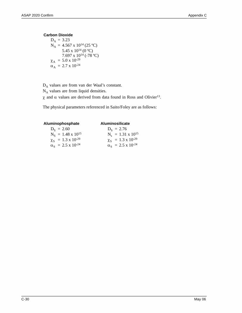
ASAP 2020 Confirm Appendix C
DA values are from van der Waal’s constant.NA values are from liquid densities.χ and α values are derived from data found in Ross and Olivier13.
The physical parameters referenced in Saito/Foley are as follows:
Carbon DioxideDA = 3.23NA = 4.567 x 10¹⁴ (25 ºC)
5.45 x 10¹⁴ (0 ºC)7.697 x 10¹⁴ (-78 ºC)
χA = 5.0 x 10⁻²⁹
αA = 2.7 x 10⁻²⁴
Aluminophosphate AluminosilicateDS = 2.60 DS = 2.76NS = 1.48 x 10¹⁵ Ns = 1.31 x 10¹⁵
χS = 1.3 x 10⁻²⁹ χS = 1.3 x 10⁻²⁹
αS = 2.5 x 10⁻²⁴ αS = 2.5 x 10⁻²⁴
C-30 May 06
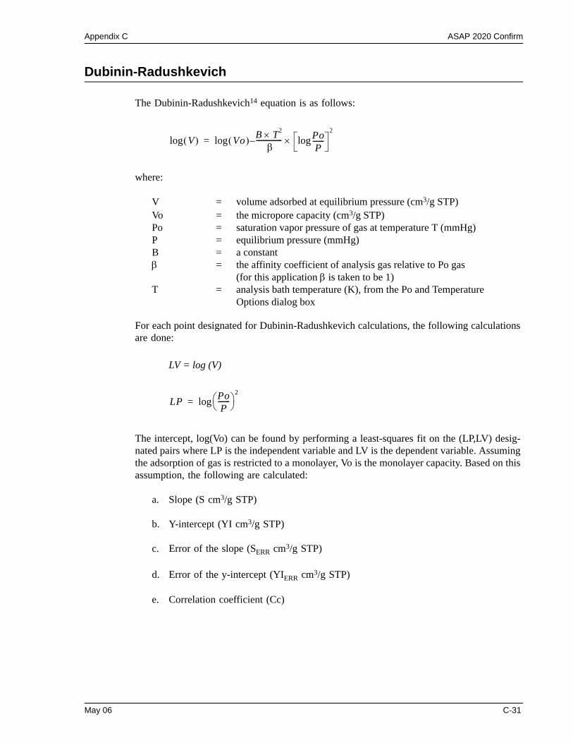
Appendix C ASAP 2020 Confirm
Dubinin-Radushkevich
The Dubinin-Radushkevich14 equation is as follows:
where:
V = volume adsorbed at equilibrium pressure (cm3/g STP)Vo = the micropore capacity (cm3/g STP)Po = saturation vapor pressure of gas at temperature T (mmHg) P = equilibrium pressure (mmHg)B = a constantβ = the affinity coefficient of analysis gas relative to Po gas
(for this application β is taken to be 1)T = analysis bath temperature (K), from the Po and Temperature
Options dialog box
For each point designated for Dubinin-Radushkevich calculations, the following calculations are done:
LV = log (V)
The intercept, log(Vo) can be found by performing a least-squares fit on the (LP,LV) desig-nated pairs where LP is the independent variable and LV is the dependent variable. Assuming the adsorption of gas is restricted to a monolayer, Vo is the monolayer capacity. Based on this assumption, the following are calculated:
a. Slope (S cm3/g STP)
b. Y-intercept (YI cm3/g STP)
c. Error of the slope (SERR cm3/g STP)
d. Error of the y-intercept (YIERR cm3/g STP)
e. Correlation coefficient (Cc)
V( )log Vo( ) B T2× β
--------------- PoP
-------log×2
–log=
LP PoP
-------⎝ ⎠⎛ ⎞
2log=
May 06 C-31
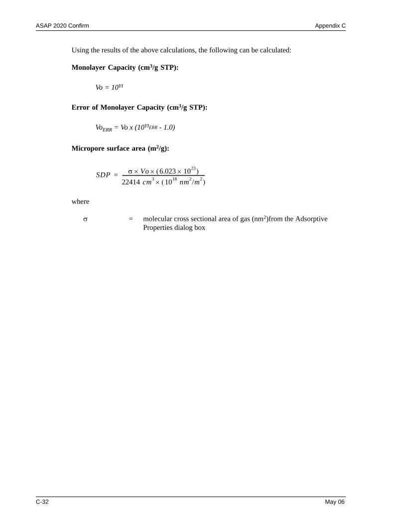
ASAP 2020 Confirm Appendix C
Using the results of the above calculations, the following can be calculated:
Monolayer Capacity (cm3/g STP):
Vo = 10YI
Error of Monolayer Capacity (cm3/g STP):
VoERR = Vo x (10YIERR - 1.0)
Micropore surface area (m2/g):
where
σ = molecular cross sectional area of gas (nm2)from the Adsorptive Properties dialog box
SDP σ Vo 6.023 1023×( )××22414 cm3 1018 nm2/m2( )×--------------------------------------------------------------------=
C-32 May 06
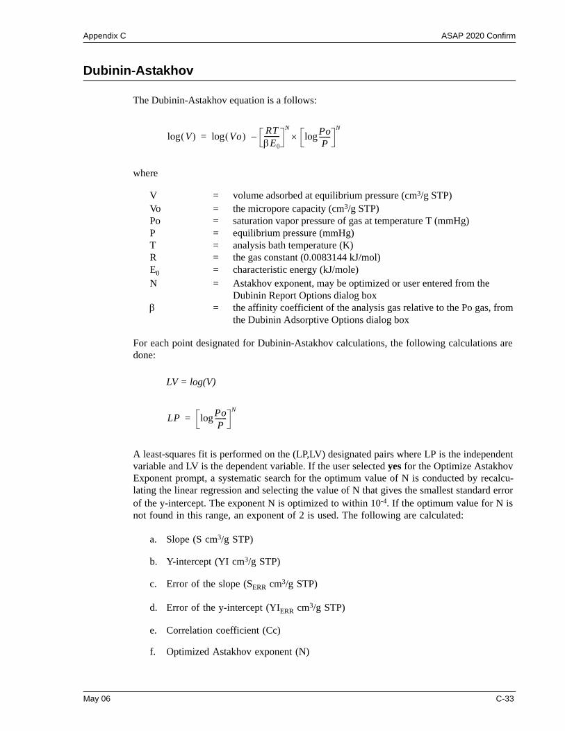
Appendix C ASAP 2020 Confirm
Dubinin-Astakhov
The Dubinin-Astakhov equation is a follows:
where
V = volume adsorbed at equilibrium pressure (cm3/g STP)Vo = the micropore capacity (cm3/g STP)Po = saturation vapor pressure of gas at temperature T (mmHg) P = equilibrium pressure (mmHg)T = analysis bath temperature (K) R = the gas constant (0.0083144 kJ/mol)E0 = characteristic energy (kJ/mole)N = Astakhov exponent, may be optimized or user entered from the
Dubinin Report Options dialog boxβ = the affinity coefficient of the analysis gas relative to the Po gas, from
the Dubinin Adsorptive Options dialog box
For each point designated for Dubinin-Astakhov calculations, the following calculations are done:
LV = log(V)
A least-squares fit is performed on the (LP,LV) designated pairs where LP is the independent variable and LV is the dependent variable. If the user selected yes for the Optimize Astakhov Exponent prompt, a systematic search for the optimum value of N is conducted by recalcu-lating the linear regression and selecting the value of N that gives the smallest standard error of the y-intercept. The exponent N is optimized to within 10-4. If the optimum value for N is not found in this range, an exponent of 2 is used. The following are calculated:
a. Slope (S cm3/g STP)
b. Y-intercept (YI cm3/g STP)
c. Error of the slope (SERR cm3/g STP)
d. Error of the y-intercept (YIERR cm3/g STP)
e. Correlation coefficient (Cc)
f. Optimized Astakhov exponent (N)
V( )log Vo( ) RTβE0---------
N PoP
-------log×N
–log=
LP PoP
-------logN
=
May 06 C-33
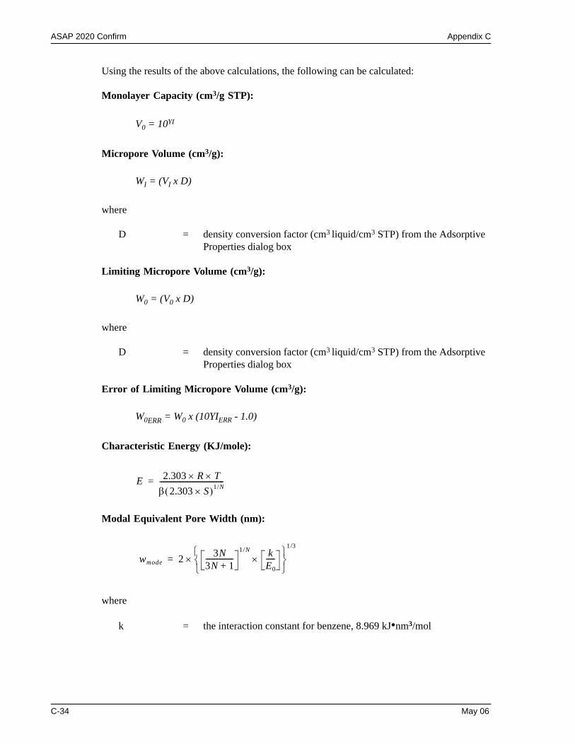
ASAP 2020 Confirm Appendix C
Using the results of the above calculations, the following can be calculated:
Monolayer Capacity (cm3/g STP):
V0 = 10YI
Micropore Volume (cm3/g):
WI = (VI x D)
where
D = density conversion factor (cm3 liquid/cm3 STP) from the Adsorptive Properties dialog box
Limiting Micropore Volume (cm3/g):
W0 = (V0 x D)
where
D = density conversion factor (cm3 liquid/cm3 STP) from the Adsorptive Properties dialog box
Error of Limiting Micropore Volume (cm3/g):
W0ERR = W0 x (10YIERR - 1.0)
Characteristic Energy (KJ/mole):
Modal Equivalent Pore Width (nm):
where
k = the interaction constant for benzene, 8.969 kJ•nm3/mol
E 2.303 R T××β 2.303 S×( )1/N-------------------------------------=
wmode 2 3N3N 1+----------------
1/N kE0-----×
⎩ ⎭⎨ ⎬⎧ ⎫
1/3
×=
C-34 May 06
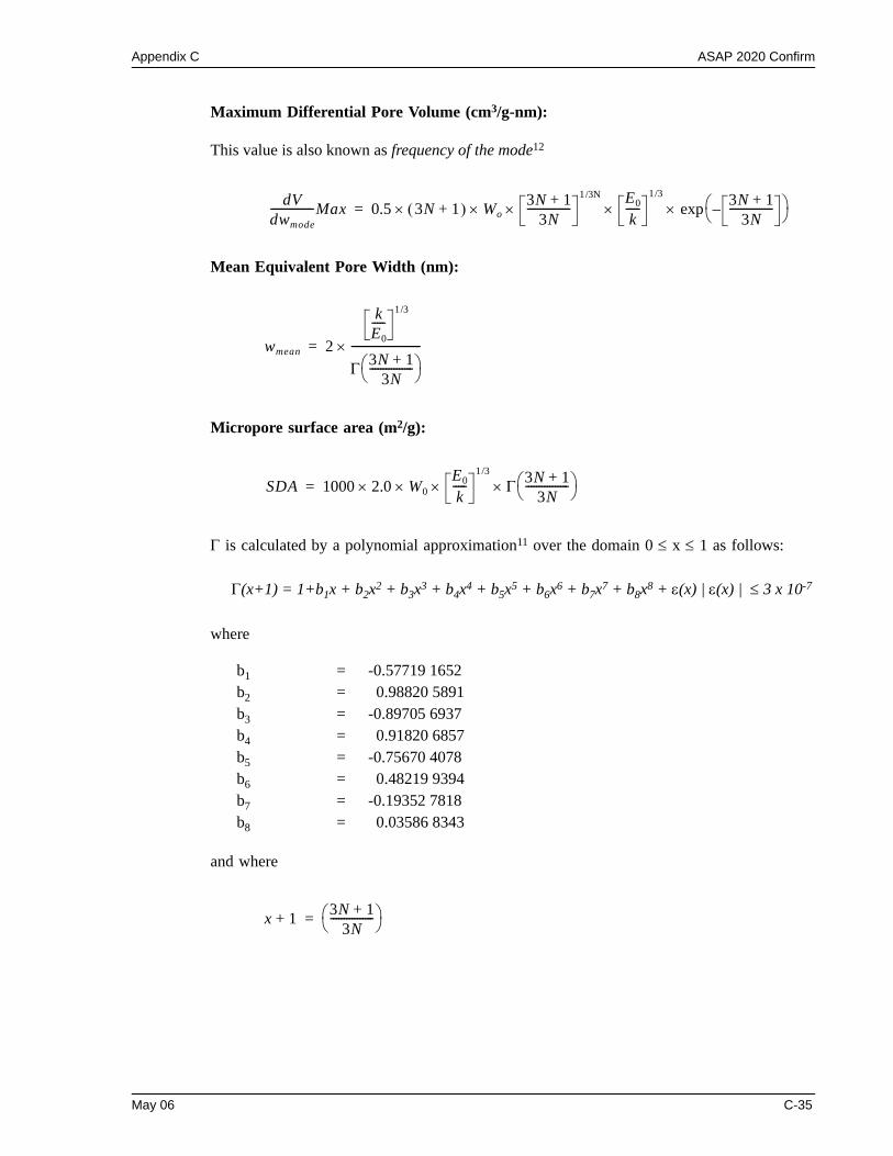
Appendix C ASAP 2020 Confirm
Maximum Differential Pore Volume (cm3/g-nm):
This value is also known as frequency of the mode12
Mean Equivalent Pore Width (nm):
Micropore surface area (m2/g):
Γ is calculated by a polynomial approximation11 over the domain 0 ≤ x ≤ 1 as follows:
Γ(x+1) = 1+b1x + b2x2 + b3x3 + b4x4 + b5x5 + b6x6 + b7x7 + b8x8 + ε(x) | ε(x) | ≤ 3 x 10⁻⁷
where
b1 = -0.57719 1652b2 = 0.98820 5891b3 = -0.89705 6937b4 = 0.91820 6857b5 = -0.75670 4078b6 = 0.48219 9394b7 = -0.19352 7818b8 = 0.03586 8343
and where
dVdwmode----------------Max 0.5 3N 1+( )× Wo× 3N 1+
3N----------------
1/3N×
E0
k-----×
1/3 3N 1+3N
----------------–⎝ ⎠⎛ ⎞exp×=
wmean 2
kE0-----
1/3
Γ 3N 1+3N
----------------⎝ ⎠⎛ ⎞
--------------------------×=
SDA 1000 2.0 W0××E0
k-----
1/3
× Γ 3N 1+3N
----------------⎝ ⎠⎛ ⎞×=
x 1+ 3N 1+3N
----------------⎝ ⎠⎛ ⎞=
May 06 C-35
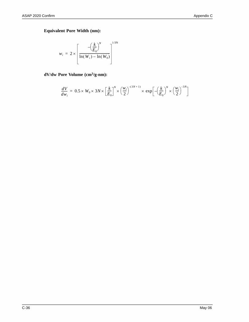
ASAP 2020 Confirm Appendix C
Equivalent Pore Width (nm):
dV/dw Pore Volume (cm3/g-nm):
wi 2
kE0-----⎝ ⎠
⎛ ⎞ N–
W( i ) W0( )ln–ln-----------------------------------------×
1/3N
=
dVdwi-------- 0.5 W0 3N k
E0-----
N×××
wi
2-----⎝ ⎠
⎛ ⎞3N 1+( )–
× kE0-----⎠
⎞ N
⎝⎛ wi
2-----⎝ ⎠
⎛ ⎞3N–
×–exp×=
C-36 May 06
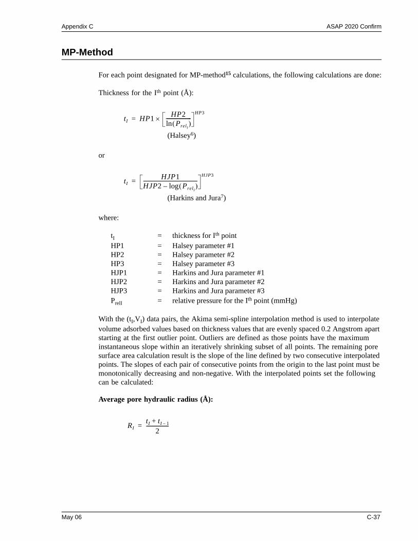
Appendix C ASAP 2020 Confirm
MP-Method
For each point designated for MP-method15 calculations, the following calculations are done:
Thickness for the Ith point (Å):
(Halsey6)
or
(Harkins and Jura7)
where:
tI = thickness for Ith point HP1 = Halsey parameter #1HP2 = Halsey parameter #2HP3 = Halsey parameter #3HJP1 = Harkins and Jura parameter #1HJP2 = Harkins and Jura parameter #2HJP3 = Harkins and Jura parameter #3PrelI = relative pressure for the Ith point (mmHg)
With the (tI,VI) data pairs, the Akima semi-spline interpolation method is used to interpolate volume adsorbed values based on thickness values that are evenly spaced 0.2 Angstrom apart starting at the first outlier point. Outliers are defined as those points have the maximum instantaneous slope within an iteratively shrinking subset of all points. The remaining pore surface area calculation result is the slope of the line defined by two consecutive interpolated points. The slopes of each pair of consecutive points from the origin to the last point must be monotonically decreasing and non-negative. With the interpolated points set the following can be calculated:
Average pore hydraulic radius (Å):
tI HP1 HP2PrelI
( )ln--------------------×
HP3=
tIHJP1
HJP2 PrelI( )log–
-------------------------------------------HJP3
=
RItI tI 1–+
2------------------=
May 06 C-37
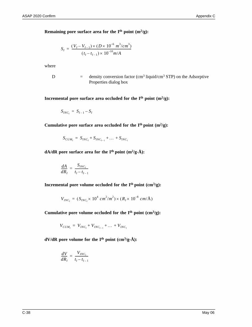
ASAP 2020 Confirm Appendix C
Remaining pore surface area for the Ith point (m2/g):
where
D = density conversion factor (cm3 liquid/cm3 STP) on the Adsorptive Properties dialog box
Incremental pore surface area occluded for the Ith point (m2/g):
Cumulative pore surface area occluded for the Ith point (m2/g):
dA/dR pore surface area for the Ith point (m2/g-Å):
Incremental pore volume occluded for the Ith point (cm3/g):
Cumulative pore volume occluded for the Ith point (cm3/g):
dV/dR pore volume for the Ith point (cm3/g-Å):
SIVI VI 1––( ) D 10 6– m3/cm3×( )×
tI tI 1––( ) 10 10– m/A×-------------------------------------------------------------------------------=
SINCISI 1– SI–=
SCUMISINCI
SINCI 1–… SINC1
+ + +=
dAdRI--------
SINCI
tI tI 1––------------------=
VINCISINCI
104 cm2/m2×( ) RI 10 8– cm/Å×( )×=
VCUMIVINCI
VINCI 1–… VINC1
+ + +=
dVdRI--------
VINCI
tI tI 1––------------------=
C-38 May 06
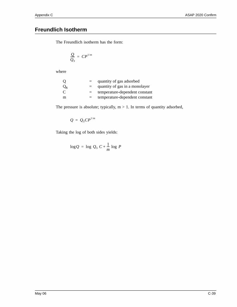
Appendix C ASAP 2020 Confirm
Freundlich Isotherm
The Freundlich isotherm has the form:
where
Q = quantity of gas adsorbedQS = quantity of gas in a monolayerC = temperature-dependent constantm = temperature-dependent constant
The pressure is absolute; typically, m > 1. In terms of quantity adsorbed,
Taking the log of both sides yields:
QQS------ CP1/m=
Q QSCP1/m=
Qlog QS C 1m---- Plog+log=
May 06 C-39
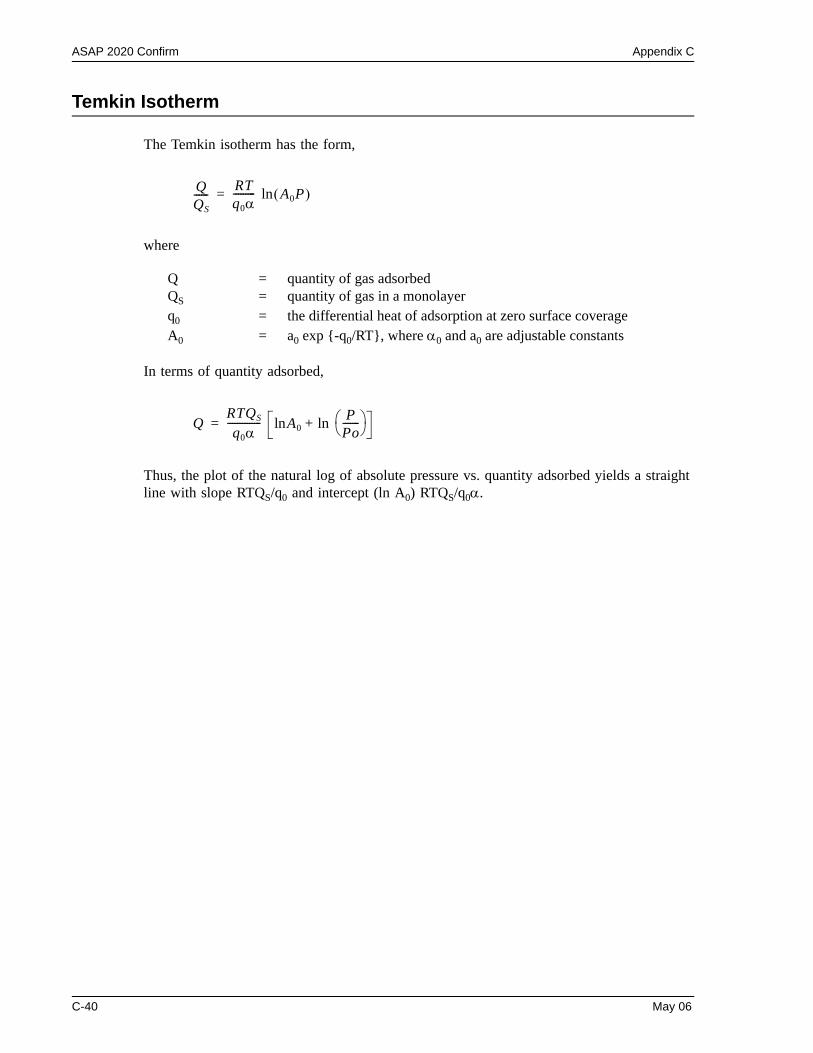
ASAP 2020 Confirm Appendix C
Temkin Isotherm
The Temkin isotherm has the form,
where
Q = quantity of gas adsorbedQS = quantity of gas in a monolayerq0 = the differential heat of adsorption at zero surface coverageA0 = a0 exp {-q0/RT}, where α0 and a0 are adjustable constants
In terms of quantity adsorbed,
Thus, the plot of the natural log of absolute pressure vs. quantity adsorbed yields a straight line with slope RTQS/q0 and intercept (ln A0) RTQS/q0α.
QQS------ RT
q0α--------- A0P( )ln=
QRTQS
q0α-------------- A0 P
Po-------⎝ ⎠
⎛ ⎞ln+ln=
C-40 May 06
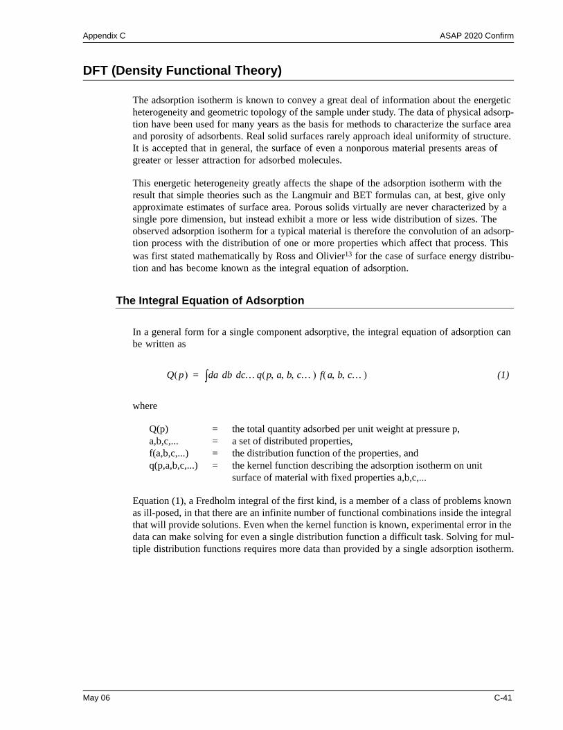
Appendix C ASAP 2020 Confirm
DFT (Density Functional Theory)
The adsorption isotherm is known to convey a great deal of information about the energetic heterogeneity and geometric topology of the sample under study. The data of physical adsorp-tion have been used for many years as the basis for methods to characterize the surface area and porosity of adsorbents. Real solid surfaces rarely approach ideal uniformity of structure. It is accepted that in general, the surface of even a nonporous material presents areas of greater or lesser attraction for adsorbed molecules.
This energetic heterogeneity greatly affects the shape of the adsorption isotherm with the result that simple theories such as the Langmuir and BET formulas can, at best, give only approximate estimates of surface area. Porous solids virtually are never characterized by a single pore dimension, but instead exhibit a more or less wide distribution of sizes. The observed adsorption isotherm for a typical material is therefore the convolution of an adsorp-tion process with the distribution of one or more properties which affect that process. This was first stated mathematically by Ross and Olivier13 for the case of surface energy distribu-tion and has become known as the integral equation of adsorption.
The Integral Equation of Adsorption
In a general form for a single component adsorptive, the integral equation of adsorption can be written as
(1)
where
Q(p) = the total quantity adsorbed per unit weight at pressure p,a,b,c,... = a set of distributed properties,f(a,b,c,...) = the distribution function of the properties, andq(p,a,b,c,...) = the kernel function describing the adsorption isotherm on unit
surface of material with fixed properties a,b,c,...
Equation (1), a Fredholm integral of the first kind, is a member of a class of problems known as ill-posed, in that there are an infinite number of functional combinations inside the integral that will provide solutions. Even when the kernel function is known, experimental error in the data can make solving for even a single distribution function a difficult task. Solving for mul-tiple distribution functions requires more data than provided by a single adsorption isotherm.
Q p( ) a d b d c…q p a b c…, , ,( ) f a b c…, ,( )d∫=
May 06 C-41
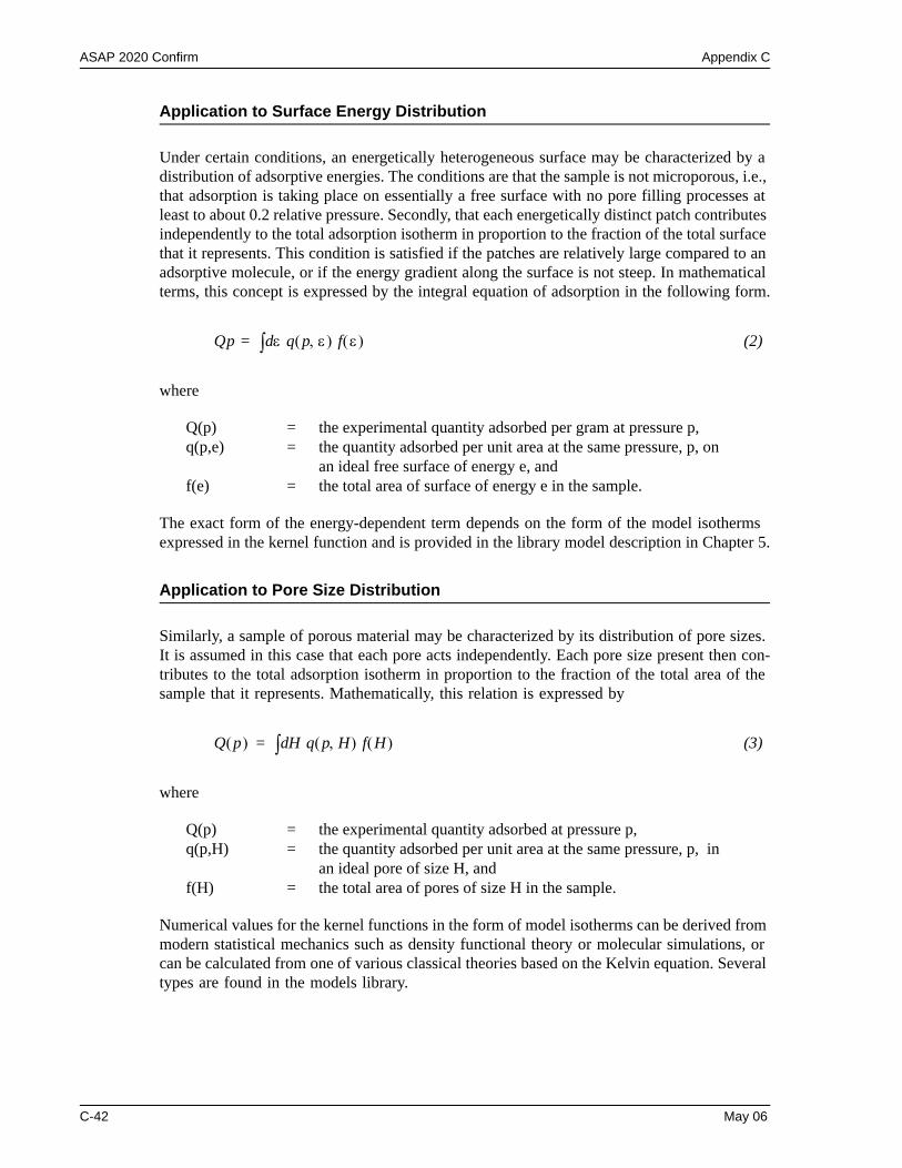
ASAP 2020 Confirm Appendix C
Application to Surface Energy Distribution
Under certain conditions, an energetically heterogeneous surface may be characterized by a distribution of adsorptive energies. The conditions are that the sample is not microporous, i.e., that adsorption is taking place on essentially a free surface with no pore filling processes at least to about 0.2 relative pressure. Secondly, that each energetically distinct patch contributes independently to the total adsorption isotherm in proportion to the fraction of the total surface that it represents. This condition is satisfied if the patches are relatively large compared to an adsorptive molecule, or if the energy gradient along the surface is not steep. In mathematical terms, this concept is expressed by the integral equation of adsorption in the following form.
(2)
where
Q(p) = the experimental quantity adsorbed per gram at pressure p,q(p,e) = the quantity adsorbed per unit area at the same pressure, p, on
an ideal free surface of energy e, and f(e) = the total area of surface of energy e in the sample.
The exact form of the energy-dependent term depends on the form of the model isotherms expressed in the kernel function and is provided in the library model description in Chapter 5.
Application to Pore Size Distribution
Similarly, a sample of porous material may be characterized by its distribution of pore sizes. It is assumed in this case that each pore acts independently. Each pore size present then con-tributes to the total adsorption isotherm in proportion to the fraction of the total area of the sample that it represents. Mathematically, this relation is expressed by
(3)
where
Q(p) = the experimental quantity adsorbed at pressure p,q(p,H) = the quantity adsorbed per unit area at the same pressure, p, in
an ideal pore of size H, and f(H) = the total area of pores of size H in the sample.
Numerical values for the kernel functions in the form of model isotherms can be derived from modern statistical mechanics such as density functional theory or molecular simulations, or can be calculated from one of various classical theories based on the Kelvin equation. Several types are found in the models library.
Qp ε q p ε,( ) f ε( )d∫=
Q p( ) H q p H,( ) f H( )d∫=
C-42 May 06
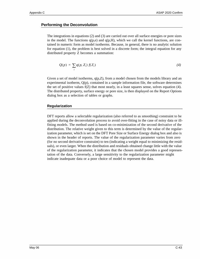
Appendix C ASAP 2020 Confirm
Performing the Deconvolution
The integrations in equations (2) and (3) are carried out over all surface energies or pore sizes in the model. The functions q(p,e) and q(p,H), which we call the kernel functions, are con-tained in numeric form as model isotherms. Because, in general, there is no analytic solution for equation (1), the problem is best solved in a discrete form; the integral equation for any distributed property Z becomes a summation:
(4)
Given a set of model isotherms, q(p,Z), from a model chosen from the models library and an experimental isotherm, Q(p), contained in a sample information file, the software determines the set of positive values f(Z) that most nearly, in a least squares sense, solves equation (4). The distributed property, surface energy or pore size, is then displayed on the Report Options dialog box as a selection of tables or graphs.
Regularization
DFT reports allow a selectable regularization (also referred to as smoothing) constraint to be applied during the deconvolution process to avoid over-fitting in the case of noisy data or ill-fitting models. The method used is based on co-minimization of the second derivative of the distribution. The relative weight given to this term is determined by the value of the regular-ization parameter, which is set on the DFT Pore Size or Surface Energy dialog box and also is shown in the header of reports. The value of the regularization parameter varies from zero (for no second derivative constraint) to ten (indicating a weight equal to minimizing the resid-uals), or even larger. When the distribution and residuals obtained change little with the value of the regularization parameter, it indicates that the chosen model provides a good represen-tation of the data. Conversely, a large sensitivity to the regularization parameter might indicate inadequate data or a poor choice of model to represent the data.
Q p( ) q p Zi,( ) f Zi( )i
∑=
May 06 C-43
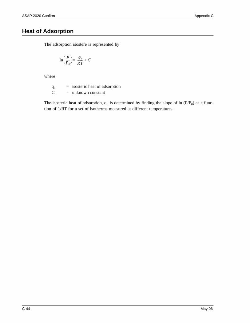
ASAP 2020 Confirm Appendix C
Heat of Adsorption
The adsorption isostere is represented by
where
qi = isosteric heat of adsorptionC = unknown constant
The isosteric heat of adsorption, q,i is determined by finding the slope of ln (P/P0) as a func-tion of 1/RT for a set of isotherms measured at different temperatures.
PP0-----⎝ ⎠
⎛ ⎞ qi
RT------- C+=ln
C-44 May 06
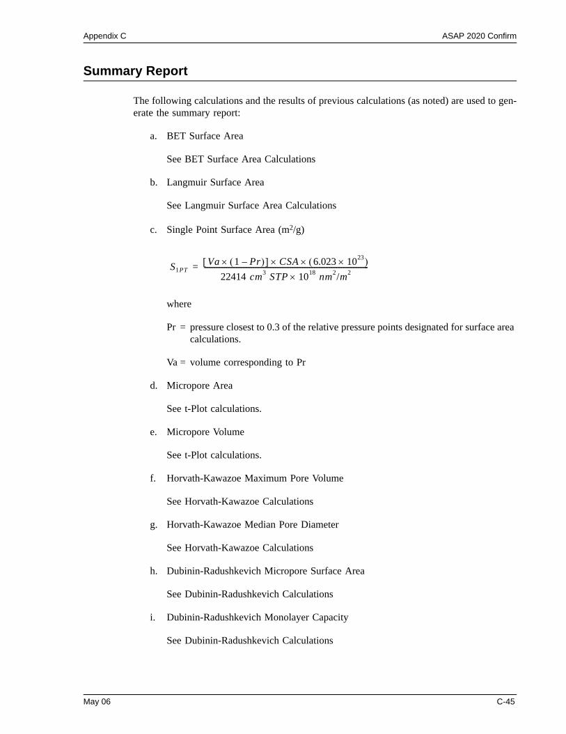
Appendix C ASAP 2020 Confirm
Summary Report
The following calculations and the results of previous calculations (as noted) are used to gen-erate the summary report:
a. BET Surface Area
See BET Surface Area Calculations
b. Langmuir Surface Area
See Langmuir Surface Area Calculations
c. Single Point Surface Area (m2/g)
where
Pr = pressure closest to 0.3 of the relative pressure points designated for surface area calculations.
Va = volume corresponding to Pr
d. Micropore Area
See t-Plot calculations.
e. Micropore Volume
See t-Plot calculations.
f. Horvath-Kawazoe Maximum Pore Volume
See Horvath-Kawazoe Calculations
g. Horvath-Kawazoe Median Pore Diameter
See Horvath-Kawazoe Calculations
h. Dubinin-Radushkevich Micropore Surface Area
See Dubinin-Radushkevich Calculations
i. Dubinin-Radushkevich Monolayer Capacity
See Dubinin-Radushkevich Calculations
S1PTVa 1 Pr–( )×[ ] CSA 6.023 1023×( )××
22414 cm3 STP 1018 nm2/m2×-------------------------------------------------------------------------------------------------=
May 06 C-45
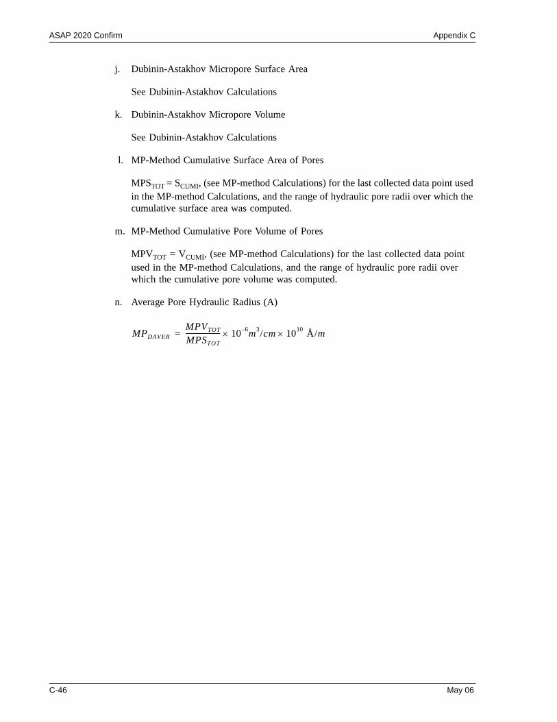
ASAP 2020 Confirm Appendix C
j. Dubinin-Astakhov Micropore Surface Area
See Dubinin-Astakhov Calculations
k. Dubinin-Astakhov Micropore Volume
See Dubinin-Astakhov Calculations
l. MP-Method Cumulative Surface Area of Pores
MPSTOT = SCUMI, (see MP-method Calculations) for the last collected data point used in the MP-method Calculations, and the range of hydraulic pore radii over which the cumulative surface area was computed.
m. MP-Method Cumulative Pore Volume of Pores
MPVTOT = VCUMI, (see MP-method Calculations) for the last collected data point used in the MP-method Calculations, and the range of hydraulic pore radii over which the cumulative pore volume was computed.
n. Average Pore Hydraulic Radius (A)
MPDAVERMPVTOT
MPSTOT-------------------- 10 6–× m3/cm 1010 Å/m×=
C-46 May 06
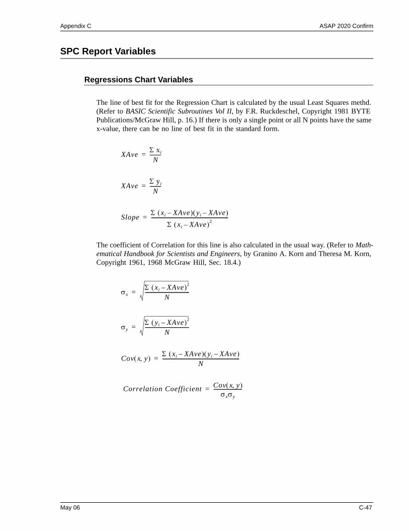
Appendix C ASAP 2020 Confirm
SPC Report Variables
Regressions Chart Variables
The line of best fit for the Regression Chart is calculated by the usual Least Squares methd. (Refer to BASIC Scientific Subroutines Vol II, by F.R. Ruckdeschel, Copyright 1981 BYTE Publications/McGraw Hill, p. 16.) If there is only a single point or all N points have the same x-value, there can be no line of best fit in the standard form.
The coefficient of Correlation for this line is also calculated in the usual way. (Refer to Math-ematical Handbook for Scientists and Engineers, by Granino A. Korn and Theresa M. Korn, Copyright 1961, 1968 McGraw Hill, Sec. 18.4.)
XAve Σ xi
N---------=
XAve Σ yi
N---------=
Slope Σ xi XAve–( ) yi XAve–( )
Σ xi XAve–( )2---------------------------------------------------------------=
σxΣ xi XAve–( )2
N------------------------------------=
σyΣ yi XAve–( )2
N------------------------------------=
Cov x y,( )Σ xi XAve–( ) yi XAve–( )
N---------------------------------------------------------------=
Correlation Coefficient Cov x y,( )σxσy
-----------------------=
May 06 C-47
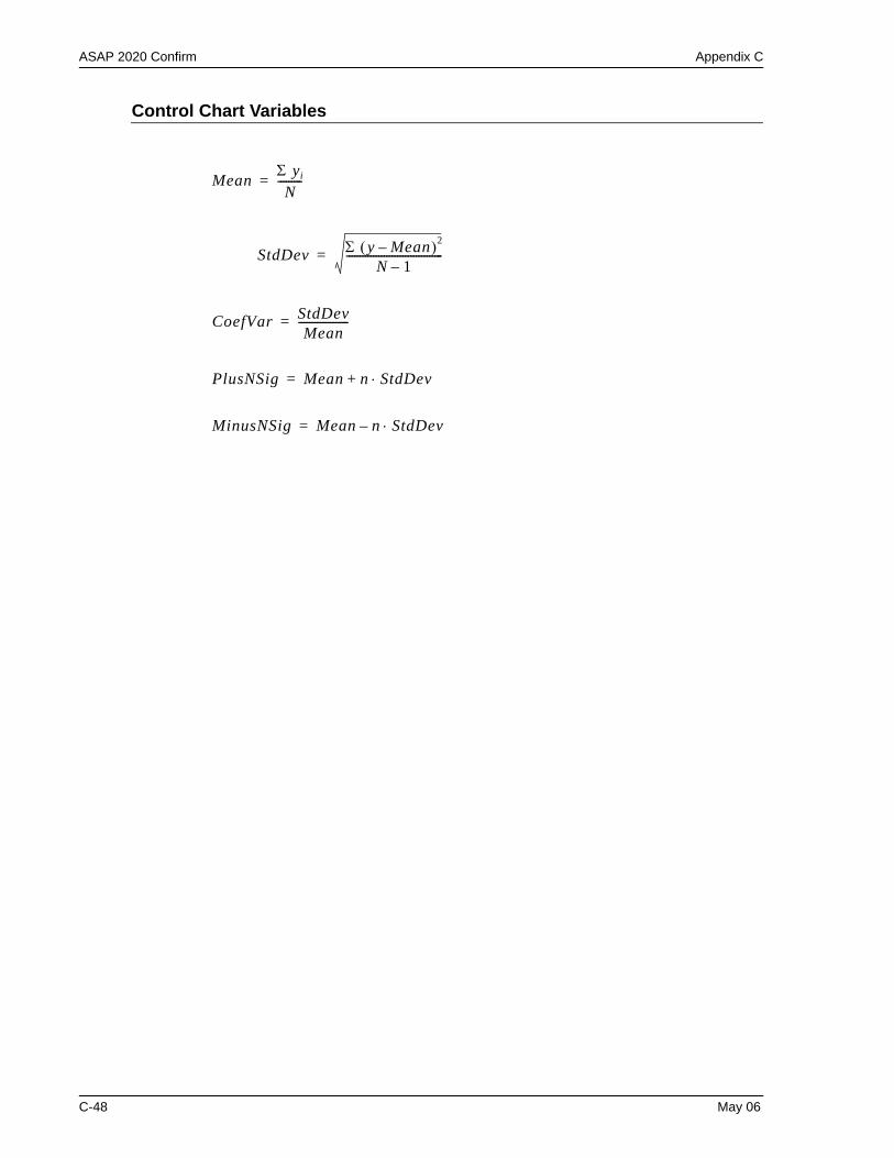
ASAP 2020 Confirm Appendix C
Control Chart Variables
Mean Σ yi
N---------=
StdDev Σ y Mean–( )2
N 1–------------------------------------=
CoefVar StdDevMean
-------------------=
PlusNSig Mean n StdDev⋅+=
MinusNSig Mean n StdDev⋅–=
C-48 May 06
Appendix C ASAP 2020 Confirm
References
1. Savitzky, A. and Golay, M.J.E., Anal. Chem. 36, 1627 (1964).
2. Blackman, R.B. and Tukey, J.W., “The Measurement of Power Spectra,” Dover (1958).
3. Brunauer, S.; Emmett, P.H.; and Teller, E., J. Am. Chem. Soc. 60, 309 (1938).
4. Langmuir, I., J. Am. Chem. Soc. 38, 2267 (1916); J. Am. Chem. Soc. 40, 1361 (1918); Phys. Rev 8, 149 (1916).
5. deBoer, J.H., et al, J. Catalysis 3, 32, 38, 44, 268 (1964); J. Catalysis 4, 319, 643, 649 (1965); Cranston, R. and Inkley, F., Adv. Catalysis 9, 143 (1957).
6. Halsey, G., J. Chem. Phys. 16, 931-937 (1948).
7. Harkins, W.D. and Jura, G., J. Chem. Phys. 11, 431 (1943).
8. Kelvin, J. (published under the name of Sir William Thomson), Phil. Mag. 42, 448-452 (1871).
9. Barrett, E.P.; Joyner, L.S.; and Halenda, P.P., J. Am. Chem. Soc. 73, 373-380 (1951).
10. Horvath, G. and Kawazoe, K., J. Chem. Eng. Japan 16(6), 470 (1983).
11. Saito, A. and Foley, H.C., AlChE Journal 37(3), 429 (1991).
12. Cheng, Linda S. and Yang, Ralph T., Chemical Engineering Science 49(16), 2599-2609 (1994).
13. Ross and Olivier, J.P., “On Physical Adsorption,” J. Wiley and Sons, New York (1964).
14. Dubinin, M., Carbon 21, 359 (1983); Dubinin, M., Progress in Surface and Membrane Science 9, 1, Academic Press, New York (1975); Dubinin, M. and Astakhov, V., Adv. Chem. Ser. 102, 69 (1971); Lamond, T. and Marsh, H., Carbon 1, 281, 293 (1964); Medek, J., Fuel 56, 131 (1977); Polanyi, M., Trans. Faraday Soc. 28, 316 (1932); Radushkevich, L., Zh. fiz. Kemi. 33, 2202 (1949); Stoeckli, H., et al, Carbon 27, 125 (1989).
15. Mikhail, R., Brunauer, S. and Bodor, E., J. Colloid and Interface Sci. 24, 45 (1968).
May 06 C-49

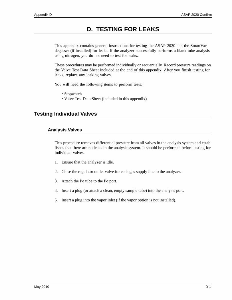
Appendix D ASAP 2020 Confirm
D. TESTING FOR LEAKS
This appendix contains general instructions for testing the ASAP 2020 and the SmartVac degasser (if installed) for leaks. If the analyzer successfully performs a blank tube analysis using nitrogen, you do not need to test for leaks.
These procedures may be performed individually or sequentially. Record pressure readings on the Valve Test Data Sheet included at the end of this appendix. After you finish testing for leaks, replace any leaking valves.
You will need the following items to perform tests:
• Stopwatch• Valve Test Data Sheet (included in this appendix)
Testing Individual Valves
Analysis Valves
This procedure removes differential pressure from all valves in the analysis system and estab-lishes that there are no leaks in the analysis system. It should be performed before testing for individual valves.
1. Ensure that the analyzer is idle.
2. Close the regulator outlet valve for each gas supply line to the analyzer.
3. Attach the Po tube to the Po port.
4. Insert a plug (or attach a clean, empty sample tube) into the analysis port.
5. Insert a plug into the vapor inlet (if the vapor option is not installed).
May 2010 D-1
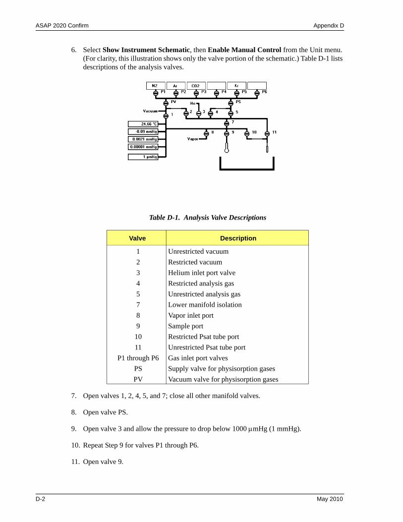
ASAP 2020 Confirm Appendix D
6. Select Show Instrument Schematic, then Enable Manual Control from the Unit menu. (For clarity, this illustration shows only the valve portion of the schematic.) Table D-1 lists descriptions of the analysis valves.
Table D-1. Analysis Valve Descriptions
7. Open valves 1, 2, 4, 5, and 7; close all other manifold valves.
8. Open valve PS.
9. Open valve 3 and allow the pressure to drop below 1000 µmHg (1 mmHg).
10. Repeat Step 9 for valves P1 through P6.
11. Open valve 9.
Valve Description
1 Unrestricted vacuum2 Restricted vacuum3 Helium inlet port valve4 Restricted analysis gas5 Unrestricted analysis gas7 Lower manifold isolation8 Vapor inlet port9 Sample port10 Restricted Psat tube port11 Unrestricted Psat tube port
P1 through P6 Gas inlet port valvesPS Supply valve for physisorption gasesPV Vacuum valve for physisorption gases
D-2 May 2010
Appendix D ASAP 2020 Confirm
12. Open valves 10 and 11.
13. Open valve 8.
14. Open valve PV.
15. Allow the system to evacuate for a minimum of one hour; a four-hour or overnight evacuation is preferred.
16. Obtain the manifold outgassing rate:
a. Close valves 3, 4, 5, 8, 9, 10, 11, and P1 through P6.
b. Evacuate manifold for another 30 minutes.
c. Take a pressure reading; record it as P1 for the manifold.
d. Close valves 1 and 2.
e. Wait 10 minutes and take another pressure reading; record it as P2 for the manifold.
f. Subtract P1 from P2 and divide the difference by 10 to obtain the outgassing rate per minute;
Outgassing rate =
Record this value as the outgassing rate for the manifold. This value should be less than 0.5 µmHg/min. for the lower manifold alone and less than 0.7 µmHg/min. for the upper and lower manifolds combined.
17. Obtain the gas inlet valve outgassing rate:
a. Open valves PS and 5; valve 7 should still be open.
b. Take a pressure reading; record it as P1 for the gas inlet valve.
c. Wait 10 minutes and take another pressure reading; record it as P2 for the gas inlet valve.
d. Subtract P1 from P2 and divide the difference by 10; record this value as the outgas-sing rate for the gas inlet valve. This value should be less than 10 µmHg/min.
Use the pressure transducer with the lowest range. For example, if you have a 1 mmHg transducer, it is the first choice. Next is the 10 mmHg transducer. If you have neither, use the Vacuum Gauge.
P2 P1–10
--------------------
May 2010 D-3
ASAP 2020 Confirm Appendix D
Valves 3 and P1 through P6
1. Open the regulator outlet valve for the gas connected to port 3.
2. Take a pressure reading; record it as P1 for valve 3.
3. Wait 10 minutes and take another pressure reading; record it as P2 for valve 3.
4. Subtract P1 from P2 and divide the difference by 10; record this value as the outgassing rate for Valve 3. This value should be less than 0.7 µmHg/min.
5. Repeat Steps 1 through 4 for valves P1 through P6 to which a gas is attached. Record the values on the Valve Test Data Worksheet in the spaces provided.
Valves PS, 5, and 7
1. Close valve PS.
2. Open valve P1 for 60 seconds, then close it.
3. Take a pressure reading; store it as P1 for valve PS.
4. Wait 10 minutes and take another pressure reading; record it as P2 for valve PS.
5. Subtract P1 from P2 and divide the difference by 10; record the value as the outgassing rate for Valve PS. This value should be less than 0.7 µmHg/min.
6. Close valve 5 (close Valve 4 if open).
7. Open valve PS.
8. Open valve P1 for 30 seconds, then close it.
9. Take a pressure reading; record it as P1 for valve 5.
10. Wait 10 minutes and take another pressure reading; record it as P2 for valve 5.
11. Subtract P1 from P2 and divide the difference by 10.; record this value as the outgassing rate for Valve 5. This value should be less than 0.7 µmHg/min.
12. Close valve 7; open valve 5.
13. Open valve P1 for 30 seconds, then close it.
14. Take a pressure reading; record it as P1 for valve 7.
15. Wait 10 minutes and take another pressure reading; record it as P2 for valve 7.
16. Subtract P1 from P2 and divide the difference by 10; record this value as the outgassing rate for Valve 7. This value should be less than 0.5 µmHg/min.
D-4 May 2010
Appendix D ASAP 2020 Confirm
Valves 1, 2, 8, 9, 10, 11, and PV
Valves 10 and 11
1. Open valve PV; wait 5 minutes (Valves PS and 5 should be open.).
2. Open valve 7; allow the system to evacuate to 10 µmHg.
3. Close valves PV, PS, and 5.
4. Open valves 1 and 2; allow the system to evacuate for 30 minutes.
Valves 1, 2, and 7 should be the only valves open at this time.
5. Remove the Po tube.
6. Take a pressure reading; record it as P1 for valves 10 and 11.
7. Wait 10 minutes and take another pressure reading; record it as P2 for valves 10 and 11.
8. Subtract P1 from P2 and divide the difference by 10; record this value as the outgassing rate for Valves 10 and 11. This value should be less than 0.7 µmHg/min.
Valve 9
9. Remove the sample tube from the analysis port.
10. Take a pressure reading; record it as P1 for valve 9.
11. Wait 10 minutes and take another pressure reading; record it as P2 for valve 9.
12. Subtract P1 from P2 and divide the difference by 10; record this value as the outgassing rate for valve 9. This should be less than 0.7 µmHg/min.
Valve 8
13. With valve 8 closed, remove the plug from the vapor inlet port on the side of the analyzer.
If the vapor accessory is installed, disconnect it from the analyzer.
14. Take a pressure reading; record it as P1 for valve 8.
15. Wait 10 minutes and take another pressure reading; record it as P2 for valve 8.
16. Subtract P1 from P2 and divide the difference by 10; record this value as the outgassing rate for valve 8. This value should be less than 0.7 µmHg/min.
17. Before proceeding, reinstall the sample tube, the Po tube, and the plug from the vapor inlet (or the vapor accessory).
May 2010 D-5
ASAP 2020 Confirm Appendix D
Valves 1, 2, and PV
18. Open valves 1 and 2.
19. Open valves 4, 5, and PS.
20. Allow the system to evacuate for 15 minutes.
21. Close valves 1 and 2. Valve PV should be closed; if not, close it.
22. Take a pressure reading; record it as P1 for valves 1, 2, and PV.
23. Wait 10 minutes and take another pressure reading; record it as P2 for valves 1, 2, and PV.
24. Subtract P1 from P2 and divide the difference by 10; record this value as the outgassing rate for valves 1, 2, and PV. This value should be less than 0.7 µmHg/min.
25. Fill the manifold to 800 mmHg with N2, then close the nitrogen port valve.
26. Close valve 4.
27. Take a pressure reading; record it as P1 for valve PV.
28. Wait 10 minutes and take another pressure reading; record it as P2 for valve PV.
29. Subtract P1 from P2 and divide the difference by 10; record this value as the outgassing rate for valve PV. This value should be less than 50 µmHg/min.
If the pressure drops more than 0.05 mmHg, close valve 5, the PV valve may be leaking.
30. Take another pressure reading; record it as P1 for valves 1 and 2.
31. Wait 10 minutes and take another pressure reading; record it as P2 for valves 1 and 2.
32. Subtract P1 from P2 and divide the difference by 10; record this value as the outgassing rate for valves 1 and 2. This value should be less than 50 µmHg/min.
If the pressure drops more than 0.05 mmHg, close valve 7, valves 1 or 2 may be leaking.
33. Take another pressure reading; record it as P1 for valve 1.
34. Wait 10 minutes and take another pressure reading; record it as P2 for valve 1.
35. Subtract P1 from P2 and divide the difference by 10; record this value as the outgassing rate for valve 1. This value should be less than 50 µmHg/min.
If the pressure drops more than 0.05 mmHg, valve 1 may be leaking.
D-6 May 2010
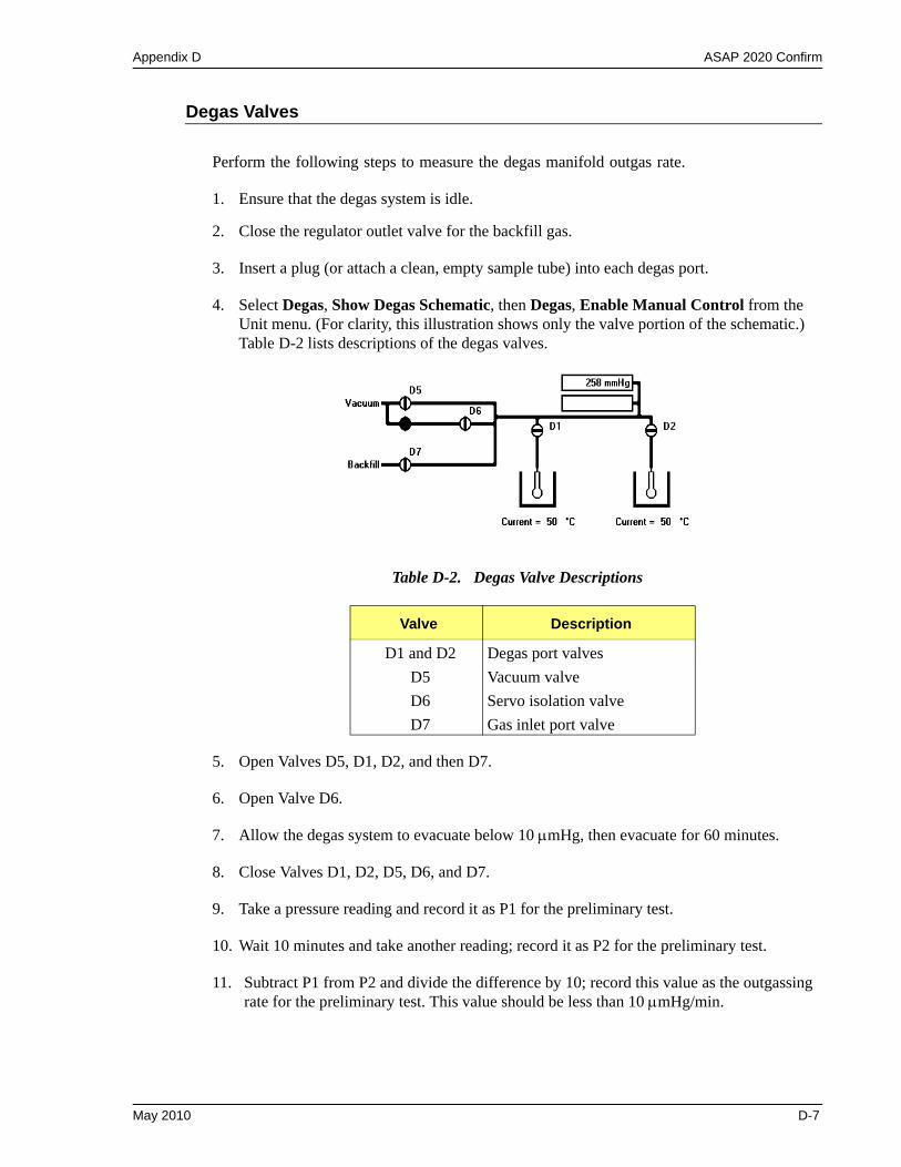
Appendix D ASAP 2020 Confirm
Degas Valves
Perform the following steps to measure the degas manifold outgas rate.
1. Ensure that the degas system is idle.
2. Close the regulator outlet valve for the backfill gas.
3. Insert a plug (or attach a clean, empty sample tube) into each degas port.
4. Select Degas, Show Degas Schematic, then Degas, Enable Manual Control from the Unit menu. (For clarity, this illustration shows only the valve portion of the schematic.) Table D-2 lists descriptions of the degas valves.
Table D-2. Degas Valve Descriptions
5. Open Valves D5, D1, D2, and then D7.
6. Open Valve D6.
7. Allow the degas system to evacuate below 10 µmHg, then evacuate for 60 minutes.
8. Close Valves D1, D2, D5, D6, and D7.
9. Take a pressure reading and record it as P1 for the preliminary test.
10. Wait 10 minutes and take another reading; record it as P2 for the preliminary test.
11. Subtract P1 from P2 and divide the difference by 10; record this value as the outgassing rate for the preliminary test. This value should be less than 10 µmHg/min.
Valve Description
D1 and D2 Degas port valvesD5 Vacuum valveD6 Servo isolation valveD7 Gas inlet port valve
May 2010 D-7
ASAP 2020 Confirm Appendix D
What To Do If You Detect a Leaking Valve
If you determine that a specific valve is leaking, remove differential pressure from the valve and continue testing the remaining valves for leaks.
Removing Differential Pressure from a Leaking Valve
1. Select either of the following actions:
• Close the regulator outlet valve for the gas supply line to the valve.• Reinstall the plug that was removed to test the valve.
2. Open the leaking valve.
3. Evacuate the analyzer until you obtain an outgas rate of less than 0.7 µmHg per minute. Refer to Testing Individual Valves on page D-1 for detailed instructions on determining the outgas rate for specific valves.
Repairing or Replacing a Leaking Valve
Whether you repair or replace a valve depends on the type of valve that is leaking.
• Valves on the Analysis manifold should be repaired• Valves on the Degas and inlet manifold should be replaced.
Repairing Valves on the Analysis Manifold
1. Backfill the manifold with nitrogen to approximately 800 mmHg.
• Close off the helium gas supply if you are repairing the helium inlet valve.• Turn off the vacuum pump system if you are repairing a vacuum valve.
2. Remove and replace the plunger and the thin gasket on the leaking valve.
As an alternative, you may repair or replace the leaking valve after removing the differential pressure on the valve. However, opening the analysis system to replace or repair a valve exposes the analyzer manifold to atmospheric gases and moisture. These gases and moisture greatly increase the time required to evacuate the analyzer and prepare it for further testing or operation.
D-8 May 2010
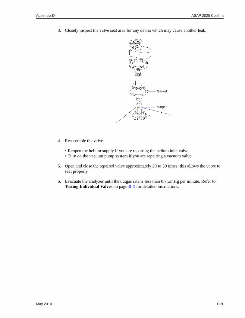
Appendix D ASAP 2020 Confirm
3. Closely inspect the valve seat area for any debris which may cause another leak.
4. Reassemble the valve.
• Reopen the helium supply if you are repairing the helium inlet valve.• Turn on the vacuum pump system if you are repairing a vacuum valve.
5. Open and close the repaired valve approximately 20 to 30 times; this allows the valve to seat properly.
6. Evacuate the analyzer until the outgas rate is less than 0.7 µmHg per minute. Refer to Testing Individual Valves on page D-1 for detailed instructions.
Plunger
Gasket
May 2010 D-9
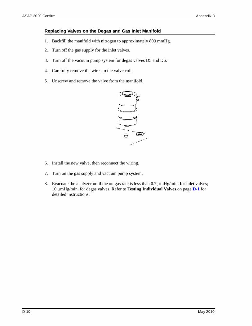
ASAP 2020 Confirm Appendix D
Replacing Valves on the Degas and Gas Inlet Manifold
1. Backfill the manifold with nitrogen to approximately 800 mmHg.
2. Turn off the gas supply for the inlet valves.
3. Turn off the vacuum pump system for degas valves D5 and D6.
4. Carefully remove the wires to the valve coil.
5. Unscrew and remove the valve from the manifold.
6. Install the new valve, then reconnect the wiring.
7. Turn on the gas supply and vacuum pump system.
8. Evacuate the analyzer until the outgas rate is less than 0.7 µmHg/min. for inlet valves; 10 µmHg/min. for degas valves. Refer to Testing Individual Valves on page D-1 for detailed instructions.
D-10 May 2010
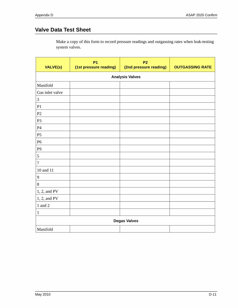
Appendix D ASAP 2020 Confirm
Valve Data Test Sheet
Make a copy of this form to record pressure readings and outgassing rates when leak-testing system valves.
VALVE(s)P1
(1st pressure reading)P2
(2nd pressure reading) OUTGASSING RATE
Analysis Valves
Manifold
Gas inlet valve
3
P1
P2
P3
P4
P5
P6
PS
5
7
10 and 11
9
8
1, 2, and PV
1, 2, and PV
1 and 2
1
Degas Valves
Manifold
May 2010 D-11

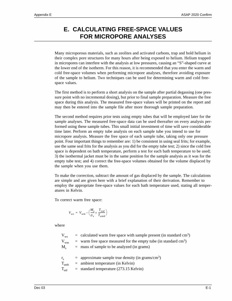
Appendix E ASAP 2020 Confirm
E. CALCULATING FREE-SPACE VALUESFOR MICROPORE ANALYSES
Many microporous materials, such as zeolites and activated carbons, trap and hold helium in their complex pore structures for many hours after being exposed to helium. Helium trapped in micropores can interfere with the analysis at low pressures, causing an “S”-shaped curve at the lower end of the isotherm. For this reason, it is recommended that you enter the warm and cold free-space volumes when performing micropore analyses, therefore avoiding exposure of the sample to helium. Two techniques can be used for determining warm and cold free-space values.
The first method is to perform a short analysis on the sample after partial degassing (one pres-sure point with no incremental dosing), but prior to final sample preparation. Measure the free space during this analysis. The measured free-space values will be printed on the report and may then be entered into the sample file after more thorough sample preparation.
The second method requires prior tests using empty tubes that will be employed later for the sample analyses. The measured free-space data can be used thereafter on every analysis per-formed using these sample tubes. This small initial investment of time will save considerable time later. Perform an empty tube analysis on each sample tube you intend to use for micropore analysis. Measure the free space of each sample tube, taking only one pressure point. Four important things to remember are: 1) be consistent in using seal frits; for example, use the same seal frits for the analysis as you did for the empty tube test; 2) since the cold free space is dependent on bath temperature, perform a test for each bath temperature to be used; 3) the isothermal jacket must be in the same position for the sample analysis as it was for the empty tube test; and 4) correct the free-space volumes obtained for the volume displaced by the sample when you use them.
To make the correction, subtract the amount of gas displaced by the sample. The calculations are simple and are given here with a brief explanation of their derivation. Remember to employ the appropriate free-space values for each bath temperature used, stating all temper-atures in Kelvin.
To correct warm free space:
where
Vws = calculated warm free space with sample present (in standard cm3)Vwm = warm free space measured for the empty tube (in standard cm3)Ms = mass of sample to be analyzed (in grams)
rs = approximate sample true density (in grams/cm3)Tamb = ambient temperature (in Kelvin)Tstd = standard temperature (273.15 Kelvin)
Vws VwmMsρs-------
TstdTamb------------× ⎠
⎞⎝⎛–=
Dec 03 E-1
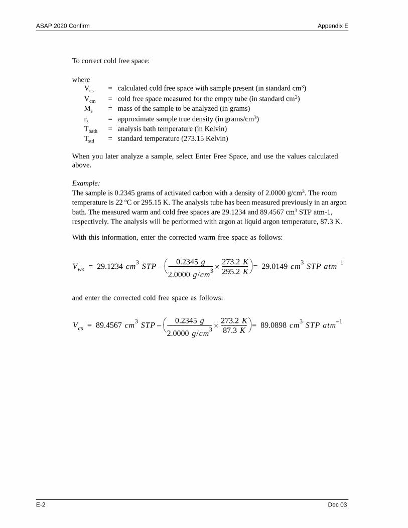
ASAP 2020 Confirm Appendix E
To correct cold free space:
whereVcs = calculated cold free space with sample present (in standard cm3)Vcm = cold free space measured for the empty tube (in standard cm3)Ms = mass of the sample to be analyzed (in grams)rs = approximate sample true density (in grams/cm3)Tbath = analysis bath temperature (in Kelvin)Tstd = standard temperature (273.15 Kelvin)
When you later analyze a sample, select Enter Free Space, and use the values calculated above.
Example:The sample is 0.2345 grams of activated carbon with a density of 2.0000 g/cm3. The room temperature is 22 ºC or 295.15 K. The analysis tube has been measured previously in an argon bath. The measured warm and cold free spaces are 29.1234 and 89.4567 cm3 STP atm-1, respectively. The analysis will be performed with argon at liquid argon temperature, 87.3 K.
With this information, enter the corrected warm free space as follows:
and enter the corrected cold free space as follows:
Vws 29.1234 cm3 STP 0.2345 g2.0000 g/cm3--------------------------------- 273.2 K
295.2 K-------------------× ⎠
⎞ 29.0149 cm3 STP atm 1–=⎝⎛–=
Vcs 89.4567 cm3 STP 0.2345 g2.0000 g/cm3--------------------------------- 273.2 K
87.3 K-------------------× ⎠
⎞ 89.0898 cm3 STP atm 1–=⎝⎛–=
E-2 Dec 03
ASAP 2020 Confirm Appendix F
F. DFT MODELS
Theories are developed by scientists in an attempt to explain a class of observed behavior. In the experimental physical sciences, theories are often expressed in terms of a model that can be visualized and described mathematically. Early models of physical adsorption were quite simple, both conceptually and mathematically, for very practical reasons — hand computa-tions were required. Today we can explore complex models that describe adsorption systems on the atomic scale of size and sub-picosecond time frame. This is not because scientists are smarter, but because of available tools. The DFT models are created by classical approaches to adsorption as well as models based on modern statistical thermodynamics.
Models Based on Statistical Thermodynamics
Included in this group are methods that model the adsorption system in terms of forces acting between individual molecules.
Theoretical Background
Traditional adsorption theories attempt to describe experimental adsorption isotherms with an isotherm equation containing a small number of parameters. At a minimum, these parameters include the extent of the surface, such as the monolayer capacity (Vm), and the molar inten-sity of the gas-surface interaction, such as the Langmuir “K” constant or the BET “C” constant. In some equations, additional parameters take into account the lateral interaction of adsorbed molecules with each other. Other theories, such as the Dubinin-Astakhov approach, also include parameters for the effect of adsorbent porosity.
Instead of this classical kinetic or phenomenological approach, we can use a molecular-based statistical thermodynamic theory that allows us to relate the adsorption isotherm to the micro-scopic properties of the system: the fluid-fluid and fluid-solid interaction energy parameters, the pore size, the pore geometry, and the temperature.
The following example is given so that you may understand how such a theory is constructed.
A clean sample of a solid material containing slit-shaped pores of a single width is placed in an evacuated space. It is kept at a fixed temperature as a known quantity of pure argon gas is admitted into the space surrounding the sample. The pressure within the space is recorded over time. In this situation, the pressure falls rapidly from its initial value and gradually approaches a steady reading, called the equilibrium pressure. The amount adsorbed corre-sponds to the quantity of gas effectively removed from the gas phase by the solid surface. A graph that plots amount adsorbed versus equilibrium pressure is called an adsorption isotherm.
Under such conditions, the argon atoms that randomly enter the pore space feel the presence of the solid surface as the action of an external attractive force (the dispersion forces or Van der Waal’s forces) and spend more time near the surface. As a result, the space near the sur-face acquires a greater average density of argon atoms than regions farther removed.
Jan 09 F-1
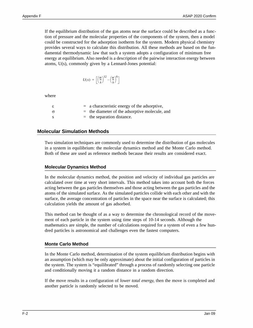
Appendix F ASAP 2020 Confirm
If the equilibrium distribution of the gas atoms near the surface could be described as a func-tion of pressure and the molecular properties of the components of the system, then a model could be constructed for the adsorption isotherm for the system. Modern physical chemistry provides several ways to calculate this distribution. All these methods are based on the fun-damental thermodynamic law that such a system adopts a configuration of minimum free energy at equilibrium. Also needed is a description of the pairwise interaction energy between atoms, U(s), commonly given by a Lennard-Jones potential:
where
ε = a characteristic energy of the adsorptive,σ = the diameter of the adsorptive molecule, ands = the separation distance.
Molecular Simulation Methods
Two simulation techniques are commonly used to determine the distribution of gas molecules in a system in equilibrium: the molecular dynamics method and the Monte Carlo method. Both of these are used as reference methods because their results are considered exact.
Molecular Dynamics Method
In the molecular dynamics method, the position and velocity of individual gas particles are calculated over time at very short intervals. This method takes into account both the forces acting between the gas particles themselves and those acting between the gas particles and the atoms of the simulated surface. As the simulated particles collide with each other and with the surface, the average concentration of particles in the space near the surface is calculated; this calculation yields the amount of gas adsorbed.
This method can be thought of as a way to determine the chronological record of the move-ment of each particle in the system using time steps of 10-14 seconds. Although the mathematics are simple, the number of calculations required for a system of even a few hun-dred particles is astronomical and challenges even the fastest computers.
Monte Carlo Method
In the Monte Carlo method, determination of the system equilibrium distribution begins with an assumption (which may be only approximate) about the initial configuration of particles in the system. The system is “equilibrated” through a process of randomly selecting one particle and conditionally moving it a random distance in a random direction.
If the move results in a configuration of lower total energy, then the move is completed and another particle is randomly selected to be moved.
U s( ) σs---⎝ ⎠
⎛ ⎞ 12 σs---⎝ ⎠
⎛ ⎞ 6–=
F-2 Jan 09
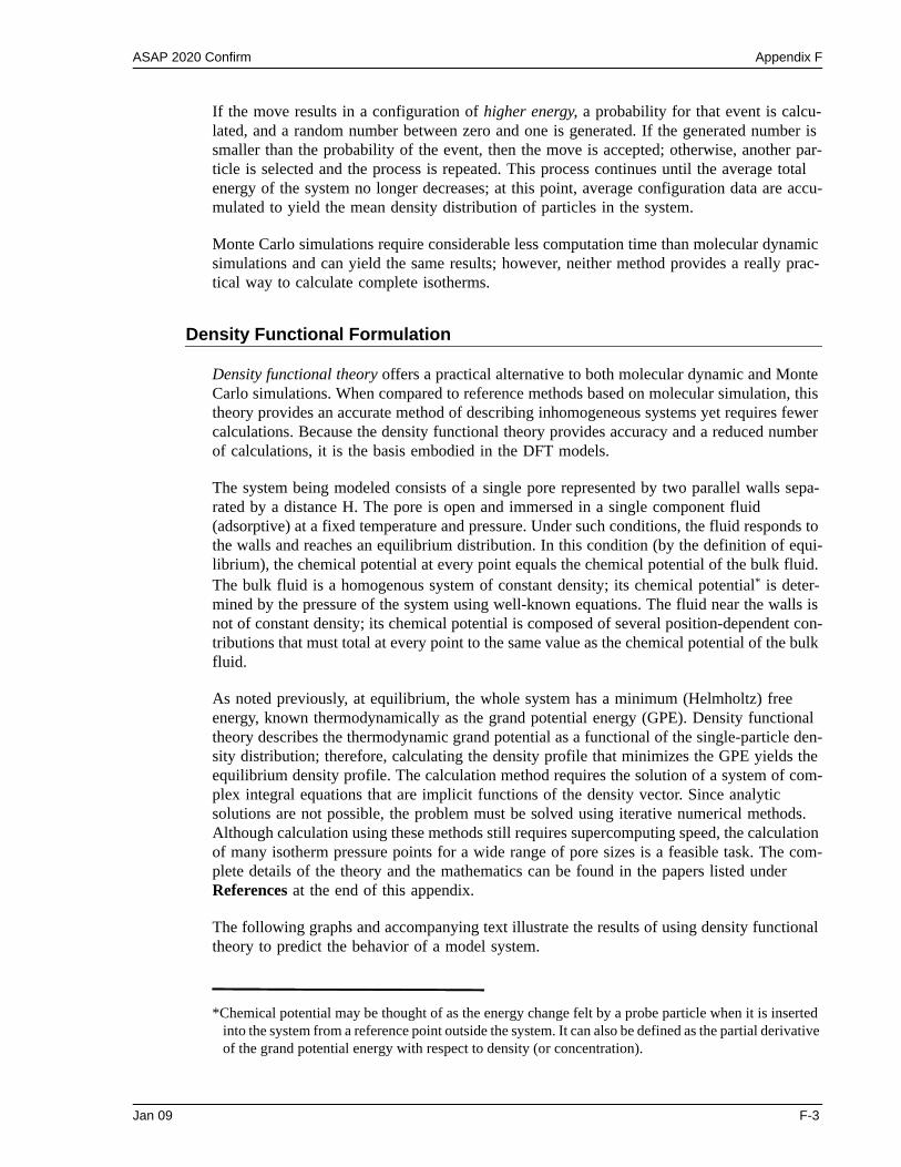
ASAP 2020 Confirm Appendix F
If the move results in a configuration of higher energy, a probability for that event is calcu-lated, and a random number between zero and one is generated. If the generated number is smaller than the probability of the event, then the move is accepted; otherwise, another par-ticle is selected and the process is repeated. This process continues until the average total energy of the system no longer decreases; at this point, average configuration data are accu-mulated to yield the mean density distribution of particles in the system.
Monte Carlo simulations require considerable less computation time than molecular dynamic simulations and can yield the same results; however, neither method provides a really prac-tical way to calculate complete isotherms.
Density Functional Formulation
Density functional theory offers a practical alternative to both molecular dynamic and Monte Carlo simulations. When compared to reference methods based on molecular simulation, this theory provides an accurate method of describing inhomogeneous systems yet requires fewer calculations. Because the density functional theory provides accuracy and a reduced number of calculations, it is the basis embodied in the DFT models.
The system being modeled consists of a single pore represented by two parallel walls sepa-rated by a distance H. The pore is open and immersed in a single component fluid (adsorptive) at a fixed temperature and pressure. Under such conditions, the fluid responds to the walls and reaches an equilibrium distribution. In this condition (by the definition of equi-librium), the chemical potential at every point equals the chemical potential of the bulk fluid. The bulk fluid is a homogenous system of constant density; its chemical potential* is deter-mined by the pressure of the system using well-known equations. The fluid near the walls is not of constant density; its chemical potential is composed of several position-dependent con-tributions that must total at every point to the same value as the chemical potential of the bulk fluid.
As noted previously, at equilibrium, the whole system has a minimum (Helmholtz) free energy, known thermodynamically as the grand potential energy (GPE). Density functional theory describes the thermodynamic grand potential as a functional of the single-particle den-sity distribution; therefore, calculating the density profile that minimizes the GPE yields the equilibrium density profile. The calculation method requires the solution of a system of com-plex integral equations that are implicit functions of the density vector. Since analytic solutions are not possible, the problem must be solved using iterative numerical methods. Although calculation using these methods still requires supercomputing speed, the calculation of many isotherm pressure points for a wide range of pore sizes is a feasible task. The com-plete details of the theory and the mathematics can be found in the papers listed under References at the end of this appendix.
The following graphs and accompanying text illustrate the results of using density functional theory to predict the behavior of a model system.
*Chemical potential may be thought of as the energy change felt by a probe particle when it is inserted into the system from a reference point outside the system. It can also be defined as the partial derivative of the grand potential energy with respect to density (or concentration).
Jan 09 F-3
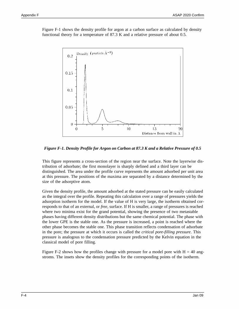
Appendix F ASAP 2020 Confirm
Figure F-1 shows the density profile for argon at a carbon surface as calculated by density functional theory for a temperature of 87.3 K and a relative pressure of about 0.5.
Figure F-1. Density Profile for Argon on Carbon at 87.3 K and a Relative Pressure of 0.5
This figure represents a cross-section of the region near the surface. Note the layerwise dis-tribution of adsorbate; the first monolayer is sharply defined and a third layer can be distinguished. The area under the profile curve represents the amount adsorbed per unit area at this pressure. The positions of the maxima are separated by a distance determined by the size of the adsorptive atom.
Given the density profile, the amount adsorbed at the stated pressure can be easily calculated as the integral over the profile. Repeating this calculation over a range of pressures yields the adsorption isotherm for the model. If the value of H is very large, the isotherm obtained cor-responds to that of an external, or free, surface. If H is smaller, a range of pressures is reached where two minima exist for the grand potential, showing the presence of two metastable phases having different density distributions but the same chemical potential. The phase with the lower GPE is the stable one. As the pressure is increased, a point is reached where the other phase becomes the stable one. This phase transition reflects condensation of adsorbate in the pore; the pressure at which it occurs is called the critical pore-filling pressure. This pressure is analogous to the condensation pressure predicted by the Kelvin equation in the classical model of pore filling.
Figure F-2 shows how the profiles change with pressure for a model pore with H = 40 ang-stroms. The insets show the density profiles for the corresponding points of the isotherm.
F-4 Jan 09
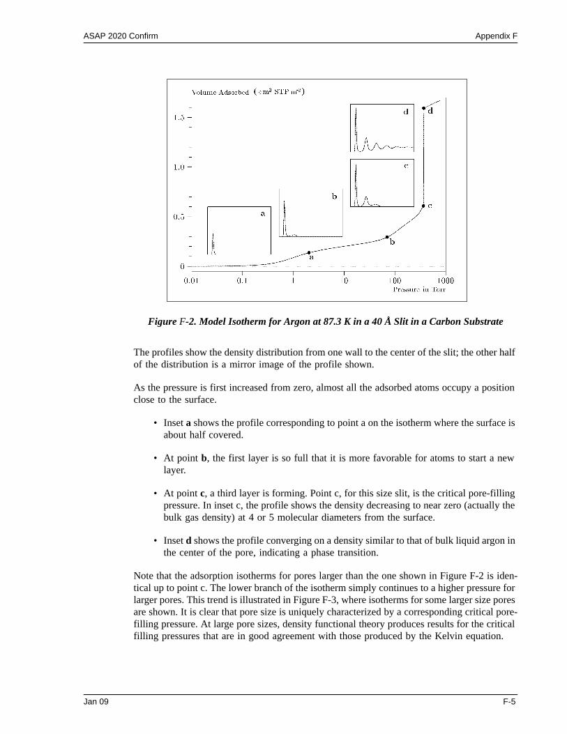
ASAP 2020 Confirm Appendix F
Figure F-2. Model Isotherm for Argon at 87.3 K in a 40 Å Slit in a Carbon Substrate
The profiles show the density distribution from one wall to the center of the slit; the other half of the distribution is a mirror image of the profile shown.
As the pressure is first increased from zero, almost all the adsorbed atoms occupy a position close to the surface.
• Inset a shows the profile corresponding to point a on the isotherm where the surface is about half covered.
• At point b, the first layer is so full that it is more favorable for atoms to start a new layer.
• At point c, a third layer is forming. Point c, for this size slit, is the critical pore-filling pressure. In inset c, the profile shows the density decreasing to near zero (actually the bulk gas density) at 4 or 5 molecular diameters from the surface.
• Inset d shows the profile converging on a density similar to that of bulk liquid argon in the center of the pore, indicating a phase transition.
Note that the adsorption isotherms for pores larger than the one shown in Figure F-2 is iden-tical up to point c. The lower branch of the isotherm simply continues to a higher pressure for larger pores. This trend is illustrated in Figure F-3, where isotherms for some larger size pores are shown. It is clear that pore size is uniquely characterized by a corresponding critical pore-filling pressure. At large pore sizes, density functional theory produces results for the critical filling pressures that are in good agreement with those produced by the Kelvin equation.
Jan 09 F-5
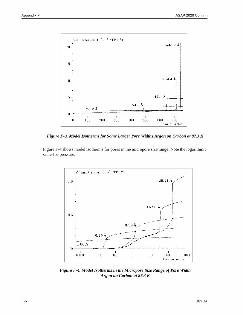
Appendix F ASAP 2020 Confirm
Figure F-3. Model Isotherms for Some Larger Pore Widths Argon on Carbon at 87.3 K
Figure F-4 shows model isotherms for pores in the micropore size range. Note the logarithmic scale for pressure.
Figure F-4. Model Isotherms in the Micropore Size Range of Pore WidthArgon on Carbon at 87.3 K
F-6 Jan 09
ASAP 2020 Confirm Appendix F
Pores of 4 Å width, barely larger than the argon atom (3.38 Å), fill at pressures below 1 mil-litorr. Pores below 15 Å fill before a monolayer is completed on the surface of the larger pores. In the micropore size range, the pore volume fills more gradually with pressure and the total shape of the isotherm is important in characterizing the pore size.
Models Included
Non-Local Density Functional Theory with Density-Independent Weights
N2 - DFT ModelAR - DFT Model
Using the methods of non-local density functional theory, two sets of isotherms have been calculated to serve as kernel functions for the characterization of porous solids from adsorp-tion data. The model isotherms are stored in binary format files. These models assume a slit-like pore geometry. The pore size range from 4.0 to 4000 Å is covered in 91 classes in a geo-metric progression. The class intervals are rounded to the nearest 0.02 molecular diameters. A model for the free or external surface is included to account for unfilled pores. Each of the 92 model isotherms has been calculated at 181 pressure points from near 1x10⁻⁶ to near 1.00 rel-ative pressure.
These models are identical to those supplied with the original DOS version of DFT software. Some slight difference from the DOS results may be noted when they are applied to the same data due to improvements in the deconvolution algorithm and better regularization of the cur-rent software.
Non-Local Density Functional Theory with Density-Dependent Weights
N2 - Modified Density Functional
Using the modified Tarazona prescription described by Olivier (refer to References, refer-ences 3 and 4), model isotherms were calculated for a wide range of adsorptive energies to a relative pressure of 0.6. The model makes no provision for pore filling in the micropore region. If the sample solid contains small mesopores, the isotherm data should be truncated (using the Select Data Points dialog box) to a suitably low relative pressure to avoid trying to fit this region; mesopore filling reports as a large area of low energy in the calculated distri-bution of adsorptive potential.
Geometry: SlitSubstrate: Carbon (graphite)Category: PorosityMethod: Nitrogen at 77 K; Argon at 87 K
Geometry: Free surfaceSubstrate: Surface energyMethod: Nitrogen at 77K
Jan 09 F-7
Appendix F ASAP 2020 Confirm
The surface energy is reported in terms of the effective Lennard-Jones interaction parameter, e, for the adsorptive/adsorbent pair divided by Boltzmann’s constant. The units are therefore degrees Kelvin.
N2 - Cylindrical Pores - Oxide SurfaceAR - Cylindrical Pores - Oxide Surface
Model isotherms were calculated using a combination of statistical mechanical calculations and experimental observations for macroporous silicas and MCM-41 mesoporous silicas as well as zeolites. The pore-filling pressures were determined as a function of the pore size from adsorption isotherms on MCM-41 materials characterized by X-ray and other tech-niques. The variation of the pore fluid density with pressure and pore size has been accounted for by density functional theory calculations. The N2 model reports pore sizes ranging from 3.8 to 387 angstroms and the AR model from 3.8 to over 500 angstroms.
N2 – Cylindrical Pores – Pillared Clay Surface (Montmorillionite)
Model isotherms were calculated using a combination of statistical thermodynamic Non-Local Density Functional Theory (NLDFT) calculations and experimental isotherms for ref-erence samples of montmorillionite.The construction method for the hybrid models was analogous to that described in the first reference below (Jaroniec et al,1999). The additional references add additional theoretical details as well as examples of the application of the model to pillared clay catalysts.This model reports pore widths from 3.8 to 387 angstroms.
Geometry: CylinderSubstrate: OxideCategory: PorosityMethod: Nitrogen at 77 K; Argon at 87 K
Reference: M. Jaroniec, M. Kruk, J.P. Olivier, and S. Koch, “A New Method for the Accurate Pore Size Analysis of MCM-41 and Other Silica-Based Mesoporous Materials,” Proceedings of COPS-V, Heidelberg, Germany (1999)
Geometry: CylinderSubstrate: Crystalline SilicateCategory: PorosityMethod: Nitrogen at 77 K
F-8 Jan 09
ASAP 2020 Confirm Appendix F
C02 - DFT Model
Model isotherms were calculated, using the non-local prescription of Tarazona, employing molecular parameters derived from the known bulk properties of carbon dioxide.
AR - Modified Density Functional Model
This model was produced in the same manner as the N2 Modified Density Functional model listed earlier, except applicable to argon adsorbed at 87.3 K.
References: Mietec Jaroniec, Michal Kruk, James P. Olivier and Stefan Koch, “A New Method for the Characterization of Mesoporous Silicas,” Proceedings of COPS-V, 1999, Studies in Surface Science, Vol 128, Characterization of porous Solids V , Unger, et al, Eds, Elsevier, Amsterdam, 2000.
James P. Olivier and Mario L. Occell, “Surface Area and Microporosity of a Pillared Interlayered Clay (PILC) from a Hybrid Density Functional Theory (DFT) Method,” The Journal of Physical Chemistry B; 2001, 105(3), 623-629.
M. L. Occelli, J. P. Olivier, J. A. Perdigon-Melon, and A. Auroux, “Surface Area, Pore Volume Distribution, and Acidity in Mesoporous Expanded Clay Catalysts from Hybrid Density Functional Theory (DFT) and Adsorption Microcalorimetry Methods,” Langmuir 2002, 18, 9816-9823.9b
James P. Olivier, “The Importance of Surface Heterogeneity in Developing Characterization Methods.” 6th International Symposium on the Character-ization of Porous Solids, Studies in Surface Science and Catalysis 144, Elsevier, 2002.
James P. Olivier and Mario L. Occelli, “Surface Area and Microporosity of Pillared Rectorite Catalysts from a Hybrid Density Functional Theory Method,” Microporous and Mesoporous Materials 2003, 57, 291-296.
Geometry: SlitSubstrate: CarbonCategory: PorosityMethod: Carbon dioxide at 273 K
Geometry: Free SurfaceSubstrate: AnyCategory: Surface energyMethod: Argon at 87 K
Jan 09 F-9
Appendix F ASAP 2020 Confirm
N2 - Tarazona NLDFT, Esf = 30.0K
Model isotherms were calculated using the prescriptions of Tarazona for density dependent weighting functions and a cylindrical pore geometry. The wall potential used is k = 30 K, typ-ical for a silica or alumina surface.
This model file is particularly useful for sizing zeolites or zeolite containing materials that have substantial micropore volume. The reported pore size range is 3.8 to 387 angstroms.
N2 - Carbon Slit Pores by NLDFTAr - Carbon Slit Pores by NLDFT
Model isotherms were calculated using the prescriptions of Tarazona for density dependent weighting functions and a slit-like pore geometry. These models are slightly different from N2-DFT and Ar-DFT models that were calculated using NLDFT with density independent weighting functions.
The reported pore size range is from 3.5 to 1000 angstroms.
N2 - Carbon Finite Pores, As=6, 2D-NLDFTAr - Carbon Finite Pores, As=6, 2D-NLDFT
Model isotherms were calculated using the prescriptions of Tarazona for density dependent weighting functions assuming 2D model of finite slit pores having a diam-eter-to-width aspect ratio of 6.
Geometry: CylinderSubstrate: OxideCategory: PorosityMethod: Nitrogen at 77 K
Reference: P. Tarazona, Phys. Rev. A 31: 2672 (1985).Idem, Phys. Rev. A 32: 3148 (1985).P. Tarazona, U. M. B. Marconi, and R. Evans, Mol. Phys. 60: 573 (1987).
Geometry: SlitSubstrate: CarbonCategory: PorosityMethod: Nitrogen at 77 K; Argon at 87K
Reference: P. Tarazona, Phys. Rev. A 31: 2672 (1985).Idem, Phys. Rev. A 32: 3148 (1985).P. Tarazona, U. M. B. Marconi, and R. Evans, Mol. Phys. 60: 573 (1987).
Geometry: Finite SlitSubstrate: CarbonCategory: PorosityMethod: Nitrogen at 77 K; Argon at 87K
F-10 Jan 09
ASAP 2020 Confirm Appendix F
This model is particularly useful for microporous carbon materials. The reported pore size range is from 3.5 to 250 angstroms.
N2 - Carbon Finite Pores, As=12, 2D-NLDFTAr - Carbon Finite Pores, As=12, 2D-NLDFT
Model isotherms were calculated using the same methods and assumptions that were used in the model above except in this model, the aspect ratio is equal to 12.
These two finite pore models may be used as a research tool in conjunction with inde-pendent analytical techniques such as high-resolution transmission electron microscopy (HRTEM) and/or X-ray diffraction (XRD) to obtain comprehensive information about the structure of studied carbon material.
Reference: Jacek Jagiello and James P. Olivier. “A simple two-dimensional NLDFT model of gas adsorption in finite carbon pores. Application to pore structure analysis.,” The Journal of Physical Chemistry C, 113(45):19382-19385, 2009.
Geometry: Finite SlitSubstrate: CarbonCategory: PorosityMethod: Nitrogen at 77 K; Argon at 87K
Reference: See above reference.
Jan 09 F-11
Appendix F ASAP 2020 Confirm
Models Based on Classical Theories
Both surface energy distribution and pore size distribution may be evaluated using classical approaches to model kernel functions for use with equation (1) of the DFT Theory in the cal-culations appendix. Be aware that the deconvolution method only provides a fitting mechanism; it does not overcome any inherent shortcomings in the underlying theory.
Surface Energy
The use of classical theories to extract adsorptive potential distribution is mostly of historical interest. At a minimum, the equation must contain a parameter dependent on adsorption energy and another dependent on monolayer capacity, or surface area. This is sufficient to permit the calculation of the set of model isotherms that is used to create a library model. The Langmuir equation has been used in the past, as have the Hill-deBoer equation and the Fowler-Guggenheim equation. All of these suffer from the fact that they only describe mono-layer adsorption, whereas the data may include contributions from multilayer formation.
Pore Size
It is well established that the pore space of a mesoporous solid fills with condensed adsorbate at pressures somewhat below the prevailing saturated vapor pressure of the adsorptive. When combined with a correlating function that relates pore size with a critical condensation pres-sure, this knowledge can be used to characterize the mesopore size distribution of the adsorbent. The correlating function most commonly used is the Kelvin equation. Refinements make allowance for the reduction of the physical pore size by the thickness of the adsorbed film existing at the critical condensation pressure. Still further refinements adjust the film thickness for the curvature of the pore wall.
The commonly used practical methods of extracting mesopore distribution from isotherm data using Kelvin-based theories, such as the BJH method, were for the most part developed decades ago and were designed for hand computation using relatively few experimental points. In general, these methods visualize the incremental decomposition of an experimental isotherm, starting at the highest relative pressure or pore size. At each step, the quantity of adsorptive involved is divided between pore emptying and film thinning processes and exactly is accounted for. This computational algorithm frequently leads to inconsistencies when carried to small mesopore sizes. If the thickness curve used is too steep, it finally will predict a larger increment of adsorptive for a given pressure increment than is actually observed; since a negative pore volume is non-physical, the algorithm must stop. Conversely, if the thickness curve used underestimates film thinning, accumulated error results in the cal-culation of an overly large volume of (possibly nonexistent) small pores.
The use of equation (1) represents an improvement over the traditional algorithm. Kernel functions corresponding to various classical Kelvin-based methods have been calculated for differing geometries and included in the list of models.
F-12 Jan 09
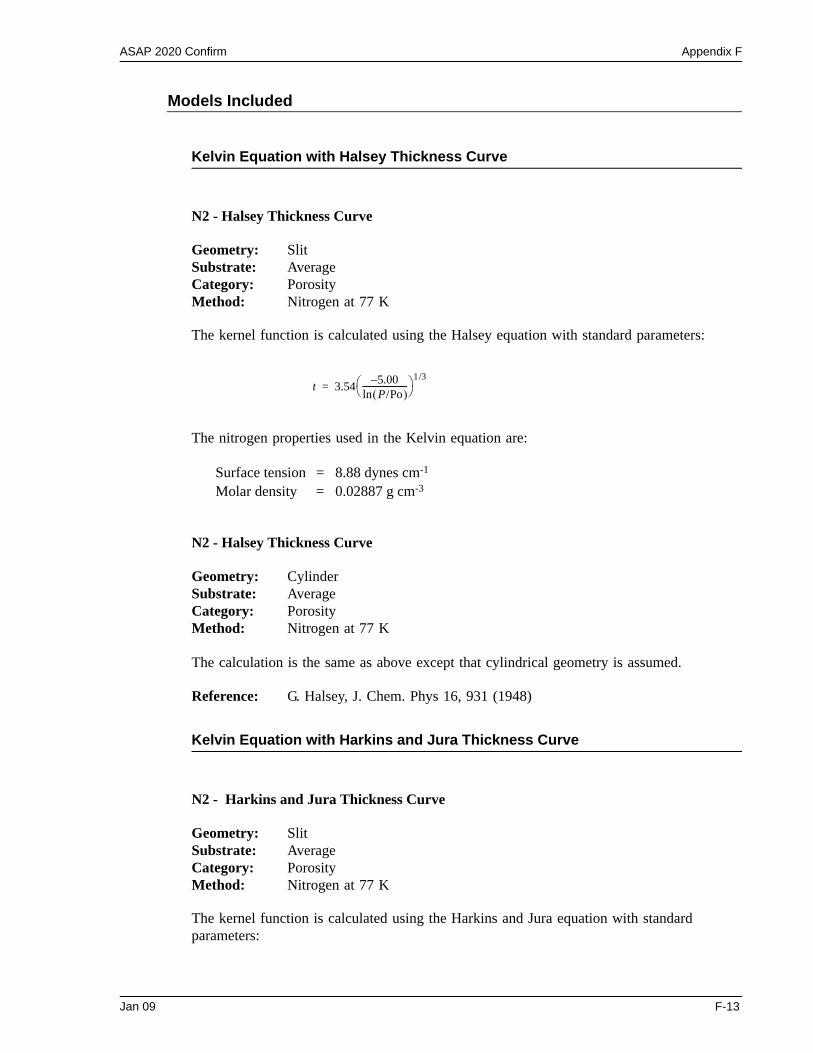
ASAP 2020 Confirm Appendix F
Models Included
Kelvin Equation with Halsey Thickness Curve
N2 - Halsey Thickness Curve
The kernel function is calculated using the Halsey equation with standard parameters:
The nitrogen properties used in the Kelvin equation are:
Surface tension = 8.88 dynes cm-1
Molar density = 0.02887 g cm-3
N2 - Halsey Thickness Curve
The calculation is the same as above except that cylindrical geometry is assumed.
Kelvin Equation with Harkins and Jura Thickness Curve
N2 - Harkins and Jura Thickness Curve
The kernel function is calculated using the Harkins and Jura equation with standard parameters:
Geometry: SlitSubstrate: AverageCategory: PorosityMethod: Nitrogen at 77 K
Geometry: CylinderSubstrate: AverageCategory: PorosityMethod: Nitrogen at 77 K
Reference: G. Halsey, J. Chem. Phys 16, 931 (1948)
Geometry: SlitSubstrate: AverageCategory: PorosityMethod: Nitrogen at 77 K
t 3.54 5.00–P/Po( )ln
----------------------⎝ ⎠⎛ ⎞ 1/3
=
Jan 09 F-13
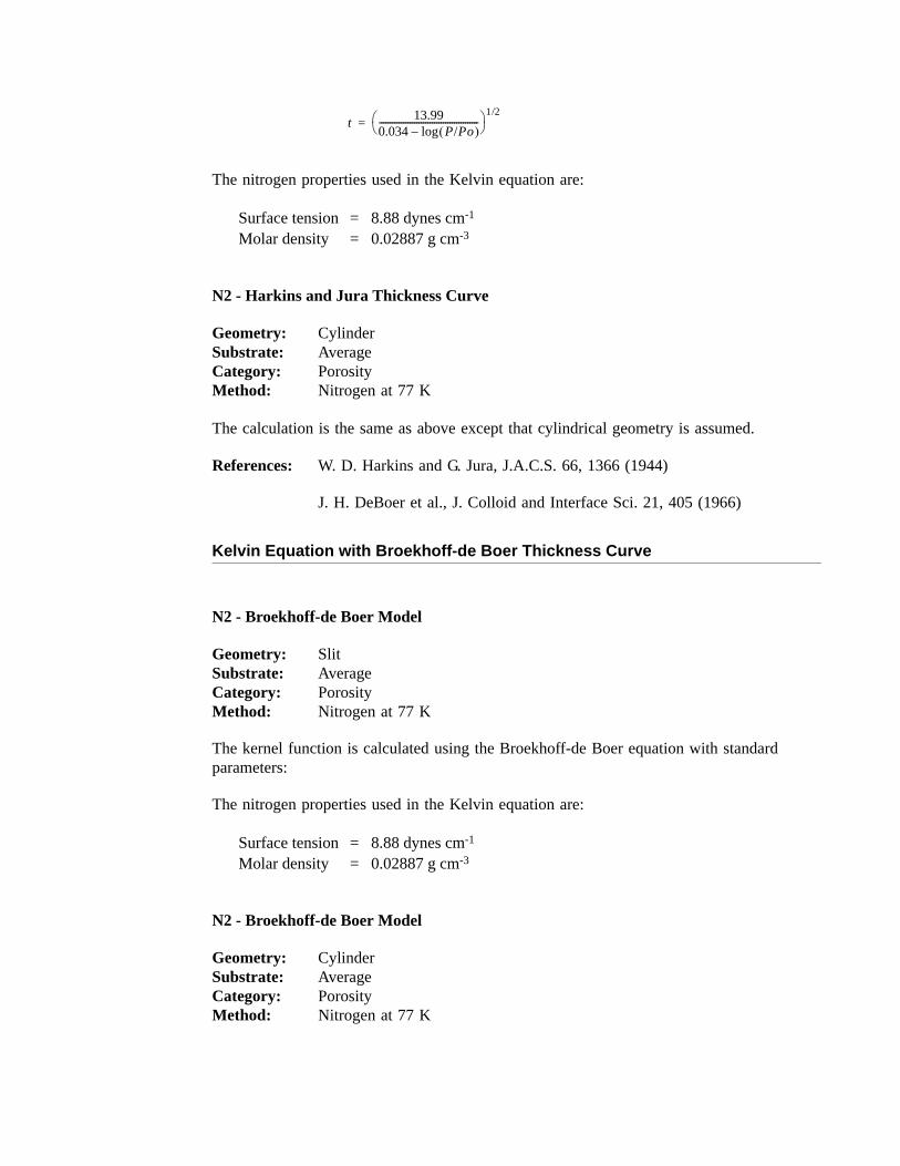
The nitrogen properties used in the Kelvin equation are:
Surface tension = 8.88 dynes cm-1
Molar density = 0.02887 g cm-3
N2 - Harkins and Jura Thickness Curve
The calculation is the same as above except that cylindrical geometry is assumed.
Kelvin Equation with Broekhoff-de Boer Thickness Curve
N2 - Broekhoff-de Boer Model
The kernel function is calculated using the Broekhoff-de Boer equation with standard parameters:
The nitrogen properties used in the Kelvin equation are:
Surface tension = 8.88 dynes cm-1
Molar density = 0.02887 g cm-3
N2 - Broekhoff-de Boer Model
Geometry: CylinderSubstrate: AverageCategory: PorosityMethod: Nitrogen at 77 K
References: W. D. Harkins and G. Jura, J.A.C.S. 66, 1366 (1944)
J. H. DeBoer et al., J. Colloid and Interface Sci. 21, 405 (1966)
Geometry: SlitSubstrate: AverageCategory: PorosityMethod: Nitrogen at 77 K
Geometry: CylinderSubstrate: AverageCategory: PorosityMethod: Nitrogen at 77 K
t 13.990.034 P/Po( )log–---------------------------------------------⎝ ⎠
⎛ ⎞ 1/2=

ASAP 2020 Confirm Appendix F
The calculation is similar to the above except that cylindrical geometry is assumed, and the film thickness depends on pore size (see reference).
Reference: Specifically, equations 20 and 21 in: J.C.P. Broekhoff and J.H. de Boer, “The Surface Area in Intermediate Pores,” Proceedings of the International Sym-posium on Surface Area Determination, D.H. Everett, R.H. Ottwill, eds., U.K. (1969)
Jan 09 F-15
References
The papers listed below provide additional information on DFT models:
1. “Determination of Pore Size Distribution from Density Functional Theoretic Models of Adsorption and Condensation within Porous Solids,” J.P. Olivier and W.B. Conklin, Micromeritics Instrument Corp; presented at the International Symposium on the Effects of Surface Heterogeneity in Adsorption and Catalysts on Solids, Kazimierz Dolny, Poland (July 1992).
2. “Classification of Adsorption Behavior: Simple Fluids in Pores of Slit-shaped Geometry,” Perla B. Balbuena and Keith E. Gubbins, Fluid Phase Equilibria, 76, 21-35, Elsevier Science Publishers, B.V., Amsterdam (1992).
3. “Modeling Physical Adsorption on Porous and Nonporous solids Using Density Functional Theory,” J.P. Olivier, Journal of Porous Materials, 3, 9-17 (1995).
4. “The Determination of Surface Energetic Heterogeneity Using Model Isotherms Calculated by Density Functional Theory,” J.P. Olivier; presented at the Fifth International Conference on the Fundamentals of Adsorption, Pacific Grove, CA (1995).
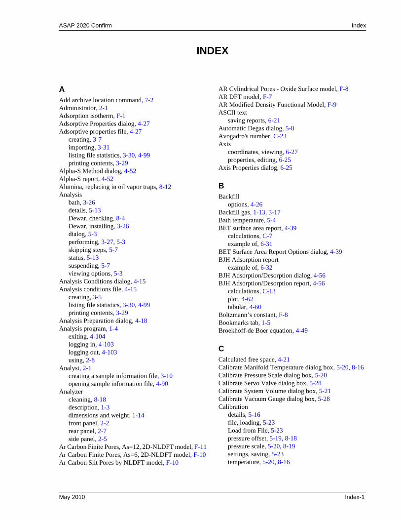
ASAP 2020 Confirm Index
INDEX
AAdd archive location command, 7-2Administrator, 2-1Adsorption isotherm, F-1Adsorptive Properties dialog, 4-27Adsorptive properties file, 4-27
creating, 3-7importing, 3-31listing file statistics, 3-30, 4-99printing contents, 3-29
Alpha-S Method dialog, 4-52Alpha-S report, 4-52Alumina, replacing in oil vapor traps, 8-12Analysis
bath, 3-26details, 5-13Dewar, checking, 8-4Dewar, installing, 3-26dialog, 5-3performing, 3-27, 5-3skipping steps, 5-7status, 5-13suspending, 5-7viewing options, 5-3
Analysis Conditions dialog, 4-15Analysis conditions file, 4-15
creating, 3-5listing file statistics, 3-30, 4-99printing contents, 3-29
Analysis Preparation dialog, 4-18Analysis program, 1-4
exiting, 4-104logging in, 4-103logging out, 4-103using, 2-8
Analyst, 2-1creating a sample information file, 3-10opening sample information file, 4-90
Analyzercleaning, 8-18description, 1-3dimensions and weight, 1-14front panel, 2-2rear panel, 2-7side panel, 2-5
Ar Carbon Finite Pores, As=12, 2D-NLDFT model, F-11Ar Carbon Finite Pores, As=6, 2D-NLDFT model, F-10Ar Carbon Slit Pores by NLDFT model, F-10
AR Cylindrical Pores - Oxide Surface model, F-8AR DFT model, F-7AR Modified Density Functional Model, F-9ASCII text
saving reports, 6-21Automatic Degas dialog, 5-8Avogadro's number, C-23Axis
coordinates, viewing, 6-27properties, editing, 6-25
Axis Properties dialog, 6-25
BBackfill
options, 4-26Backfill gas, 1-13, 3-17Bath temperature, 5-4BET surface area report, 4-39
calculations, C-7example of, 6-31
BET Surface Area Report Options dialog, 4-39BJH Adsorption report
example of, 6-32BJH Adsorption/Desorption dialog, 4-56BJH Adsorption/Desorption report, 4-56
calculations, C-13plot, 4-62tabular, 4-60
Boltzmann’s constant, F-8Bookmarks tab, 1-5Broekhoff-de Boer equation, 4-49
CCalculated free space, 4-21Calibrate Manifold Temperature dialog box, 5-20, 8-16Calibrate Pressure Scale dialog box, 5-20Calibrate Servo Valve dialog box, 5-28Calibrate System Volume dialog box, 5-21Calibrate Vacuum Gauge dialog box, 5-28Calibration
details, 5-16file, loading, 5-23Load from File, 5-23pressure offset, 5-19, 8-18pressure scale, 5-20, 8-19settings, saving, 5-23temperature, 5-20, 8-16
May 2010 Index-1
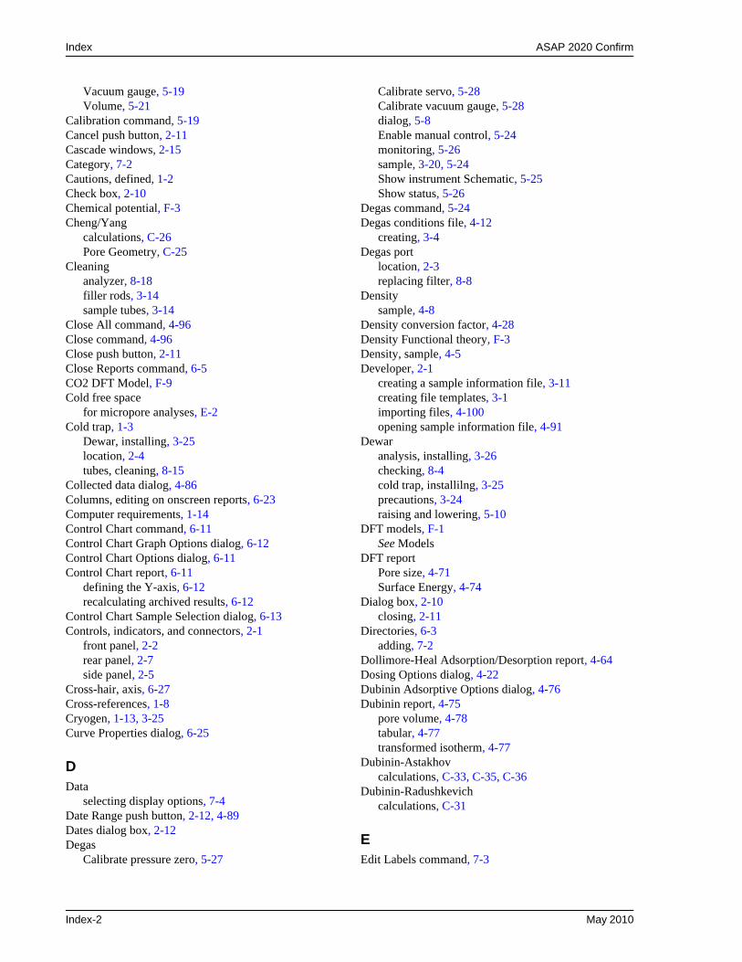
Index ASAP 2020 Confirm
Vacuum gauge, 5-19Volume, 5-21
Calibration command, 5-19Cancel push button, 2-11Cascade windows, 2-15Category, 7-2Cautions, defined, 1-2Check box, 2-10Chemical potential, F-3Cheng/Yang
calculations, C-26Pore Geometry, C-25
Cleaninganalyzer, 8-18filler rods, 3-14sample tubes, 3-14
Close All command, 4-96Close command, 4-96Close push button, 2-11Close Reports command, 6-5CO2 DFT Model, F-9Cold free space
for micropore analyses, E-2Cold trap, 1-3
Dewar, installing, 3-25location, 2-4tubes, cleaning, 8-15
Collected data dialog, 4-86Columns, editing on onscreen reports, 6-23Computer requirements, 1-14Control Chart command, 6-11Control Chart Graph Options dialog, 6-12Control Chart Options dialog, 6-11Control Chart report, 6-11
defining the Y-axis, 6-12recalculating archived results, 6-12
Control Chart Sample Selection dialog, 6-13Controls, indicators, and connectors, 2-1
front panel, 2-2rear panel, 2-7side panel, 2-5
Cross-hair, axis, 6-27Cross-references, 1-8Cryogen, 1-13, 3-25Curve Properties dialog, 6-25
DData
selecting display options, 7-4Date Range push button, 2-12, 4-89Dates dialog box, 2-12Degas
Calibrate pressure zero, 5-27
Calibrate servo, 5-28Calibrate vacuum gauge, 5-28dialog, 5-8Enable manual control, 5-24monitoring, 5-26sample, 3-20, 5-24Show instrument Schematic, 5-25Show status, 5-26
Degas command, 5-24Degas conditions file, 4-12
creating, 3-4Degas port
location, 2-3replacing filter, 8-8
Densitysample, 4-8
Density conversion factor, 4-28Density Functional theory, F-3Density, sample, 4-5Developer, 2-1
creating a sample information file, 3-11creating file templates, 3-1importing files, 4-100opening sample information file, 4-91
Dewaranalysis, installing, 3-26checking, 8-4cold trap, installilng, 3-25precautions, 3-24raising and lowering, 5-10
DFT models, F-1See Models
DFT reportPore size, 4-71Surface Energy, 4-74
Dialog box, 2-10closing, 2-11
Directories, 6-3adding, 7-2
Dollimore-Heal Adsorption/Desorption report, 4-64Dosing Options dialog, 4-22Dubinin Adsorptive Options dialog, 4-76Dubinin report, 4-75
pore volume, 4-78tabular, 4-77transformed isotherm, 4-77
Dubinin-Astakhovcalculations, C-33, C-35, C-36
Dubinin-Radushkevichcalculations, C-31
EEdit Labels command, 7-3
Index-2 May 2010
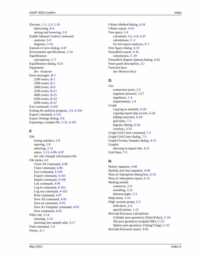
ASAP 2020 Confirm Index
Elevator, 1-3, 2-3, 5-10lubricating, 8-4raising and lowering, 5-9
Enable Manual Control commandanalyzer, 5-9degasser, 5-24
Entered t-Curve dialog, 4-47Environment specificaitons, 1-14Equilibration
calculations, C-5Equilibration dialog, 4-25Equipment
See AnalyzerError messages, B-1
2200 series, B-12300 series, B-12400 series, B-62500 series, B-174000 series, B-256200 series, B-436500 series, B-47
Exit command, 4-104Exiting the analysis program, 2-9, 4-104Export command, 4-101Export Settings dialog, 5-6Exporting a sample file, 3-32, 4-101
FFile
listing statistics, 2-9opening, 2-9selecting, 2-12status, 2-13, 4-89, 4-97See also Sample information file
File menu, 4-1Close All command, 4-96Close command, 4-96Exit command, 4-104Export command, 4-101Import command, 4-100List command, 4-99Log in command, 4-103Log out command, 4-103Print command, 4-97Save All command, 4-95Save as command, 4-93Save As Template command, 4-95Save command, 4-93
Filler rod, 3-14cleaning, 3-14inserting into sample tube, 3-17
Find command, 1-9Forms, A-1
f-Ratio Method dialog, 4-54f-Ratio report, 4-54Free space, 5-4
calculated, 4-5, 4-8, 4-21calculations, C-3for micropore analyses, E-1
Free Space dialog, 4-19Freundlich report, 4-42
calculations, C-39Freundlich Report Options dialog, 4-42Front panel description, 2-2Function keys
See Shortcut keys
GGas
connection ports, 2-5regulator pressure, 3-27regulators, 1-4requirements, 1-4
Graphcopying as metafile, 6-26copying report data as text, 6-26editing onscreen, 6-24grid lines, 7-5legend, editing, 6-26overlays, 3-33
Graph Grid Lines command, 7-5Graph Grid Lines dialog, 7-5Graph Overlay Samples dialog, 4-31Graphic
showing in report title, 4-31Grid lines, 7-5
HHalsey equation, 4-48Harkins and Jura equation, 4-49Heat of Adsorption dialog box, 6-14Heat of Adsorption report, 6-14Heating mantle
connector, 2-4installing, 3-21thermocouple, 2-3
Help menu, 2-16High vacuum pump, 2-3
indicators, 2-4specifications, 1-12
Horvath-Kawazoe calculationsCylinder pore geometry (Saito/Foley), C-24Slit pore geometry (original HK), C-23Sphere pore geometry (Cheng/Yang), C-25
Horvath-Kawazoe report, 4-65
May 2010 Index-3
Index ASAP 2020 Confirm
calculations, C-23plot, 4-69tabular, 4-68
IImport command, 4-100Importing files, 3-31, 4-100Index, online, 1-8Indicators, 2-1Information bar, 2-10Insert Predefined Pressures dialog, 4-17Insert Pressure Range dialog, 4-16Instrument schematic
analyzer, 5-12degasser, 5-24
Interaction parameter, C-26Isosteric heat of adsorption, 6-14Isotherm, F-1Isotherm data, exporting, 3-32Isotherm report, 4-36
example of, 6-29Isotherm Report Options dialog, 4-36Isothermal jacket, 1-3, 1-13, 3-22, 4-10
KKernel function, F-12, F-13Kruk-Jaroniec-Sayari Equation, 4-48
LLabels, sample file, editing, 7-3Langmuir surface area report, 4-39
calculations, C-9Langmuir Surface Area Report Options dialog, 4-39Leak test
blank tube analysis (nitrogen), D-1Data sheet for recording values, D-11removing differential pressure, D-8Valve 9, D-5Valves 10 and 11, D-5Valves P1 through P6, D-4Valves PS, 5, and 7, D-4
Legend Properties dialog, 6-26Lennard-Jones, F-2, F-8Links, 1-7List command, 4-99Listing file statistics, 3-30, 4-99Load from File command, 5-23Log in, 2-8Log in command, 4-103Log out command, 4-103
MMain Menu bar, 2-14Maintenance, 8-1Manifold temperature
calibrating, 5-20, 8-16Manual
See Operator’s manualManual control, 5-9
enabling for analyzer, 5-9MCM-41 materials, F-8Menu structure, 2-14Messages
See Error MessagesMetafile, copying graph as, 6-26Micropore analyses
free-space values, E-1Models, F-1
Ar Carbon finite pores by NLDFT, As=12, F-11Ar Carbon finite pores by NLDFT, As=6, F-10Ar Carbon slit pores by NLDFT, F-10AR Cylindrical Pores - Oxide Surface, F-8AR DFT model, F-7AR Modified Density Functional, F-9based on classical theories, F-12based on statistical thermodynamics, F-1CO2 DFT Model, F-9N2 Broekhoff-de Boer Model, F-14N2 Carbon finite pores by NLDFT, As=12, F-11N2 Carbon finite pores by NLDFT, As=6, F-10N2 Carbon slit pores by NLDFT, F-10N2 Cylindrical Pores - Oxide Surface, F-8N2 Cylindrical Pores - Pillared Clay Surface, F-8N2 DFT model, F-7N2 Halsey Thickness Curve, F-13N2 Harkins and Jura Thickness Curve, F-13, F-14N2 Harkins and Jura Thickness Curve model, F-13N2 Modified Density Functional, F-7N2 Tarazona NLDFT, Esf = 30.0K, F-10
Molecular dynamics, F-2Molecular simulation methods, F-2Monte Carlo, F-2Montmorillionite, F-8MP-Method report, 4-80
calculations, C-37pore volume/pore area, 4-82tabular, 4-82
NN2 Broekhoff-de Boer model, F-14N2 Broekhoff-de Boer Model model, F-14N2 Carbon Finite Pores, As=12, 2D-NLDFT model,
F-11N2 Carbon Finite Pores, As=6, 2D-NLDFT model, F-10
Index-4 May 2010
ASAP 2020 Confirm Index
N2 Carbon Slit Pores by NLDFT model, F-10N2 Cylindrical Pores - Oxide Surface model, F-8N2 Cylindrical Pores - Pillared Clay Surface model, F-8N2 DFT model, F-7N2 Halsey Thickness Curve model, F-13N2 Harkins and Jura Thickness Curve model, F-14N2 Modified Density Functional model, F-7N2 Tarazona NLDFT, Esf = 30.0K model, F-10Non-ideality factor, 4-10Notes, defined, 1-2
OOil vapor traps, replacing alumina, 8-12Online manual
cross references, 1-8index, 1-8printing options, 1-10using, 1-5See also Operator’s manual
Open Report command, 6-5Operator’s manual
conventions used, 1-2online, 1-5organization, 1-1See also Online manual
Options menuAdd Archive Location command, 7-2description, 7-1Edit Labels command, 7-3Graph Grid Lines command, 7-5Update File List command, 7-4
Options report, 4-84example of, 6-34
Ordering information, 9-1Overlays
for multiple samples, 3-34generating, 3-33
PParameter file, 4-4, 4-92
Adsorptive properties, 4-27creating, 3-3, 4-3creating templates, 3-2importing, 3-31, 4-100listing file statistics, 3-30, 4-99printing contents, 3-29Report options, 4-30
Parts, ordering, 9-1Pass/Fail Options dialog, 4-35Password, 2-8
changing, 4-103logging in, 4-103
Po and Temperature Options dialog, 4-21Po port, 2-4Pore filling pressure, F-4Pore Geometry
cylinder (Saito-Foley), C-24slit (original Horvath-Kawazoe), C-23sphere (Cheng/Yang), C-25
Pore size, F-12Port filter, degas, 8-8Ports
gas connection, 2-5Pressure
relative, calculations, C-1, C-2Pressure offset
calibrating, 8-18Pressure scale
calibrating, 5-20, 8-19calibrating (Degasser), 5-27
Pressure table, 4-16Pressure zero
calibrating, 5-27Preventive maintenance schedule, 8-3Print command, 4-97Printing file contents, 3-29Prompts, sample information, 7-3Psat vs. Temperature Table dialog, 4-28Push buttons, 2-11
RRadio button, 2-10Rate of Adsorption, 6-17Regression report, 6-7
recalculaing SPC values, 6-8selecting X- and Y-Axes variables, 6-8
Regression Report command, 6-7Regression Report Options dialog, 6-7Regression Report Sample Selection dialog, 6-8Regulators, gas, 1-4Replace push button, 2-11Report
closing, 2-9, 6-5Control Chart, 6-11displaying company logo in title, 4-31Dollimore-Heal, 4-64examples, 6-27generated automatically, 5-5generating, 6-3generating automatically after analysis, 3-28graphs, editing onscreen, 6-24header, 6-18Heat of Adsorption, 6-14Isotherm, 6-29legend, editing, 6-26
May 2010 Index-5
Index ASAP 2020 Confirm
onscreen, 6-18onscreen, shortcut menus for, 6-23Regression, 6-7saving in other formats, 6-21starting, 2-9Statistical Process Control (SPC), 6-6title, 4-30Validation, 4-85zoom feature, 6-26
Report button, 6-10Report options dialog, 4-30Report options file, 3-8, 4-30
creating, 3-8importing, 3-31listing file statistics, 3-30, 4-99printing contents, 3-29
Report Pressure Table dialog, 4-40Reports menu, 6-1
Close Reports command, 6-5Control Chart command, 6-11description, 6-1Heat of Adsorption command, 6-14Open Report command, 6-5Rate of Adsorption command, 6-17Regression Report command, 6-7SPC Report Options command, 6-6Start Report command, 6-3
Revert, 4-5, 4-9RS232 port, 2-6
SSaito-Foley
calculations, C-24Pore Geometry, C-24
Sampledegassing, 3-20, 5-24density, 4-8determining amount to use, 3-18determining weight, 3-18preparing, 3-13
Sample Analysis command, 5-3Sample Backfill Options dialog, 4-25Sample Information file
Analyst, 4-4Sample information file
creating, 4-3creating a template for, 3-1creating, Analyst, 3-10creating, Developer, 3-11Developer, 4-7editing labels for, 7-3exporting, 3-32, 4-101importing, 3-31, 4-100
listing file statistics, 3-30, 4-99opening, 4-88printing contents, 3-29revert to previous version, 4-5, 4-9versions, 4-5, 4-9
Sample Log report, 4-84Sample log report
example of, 6-35Sample port, 2-4Sample template
SeeSample tube, 3-13
cleaning, 3-14displayed on schematic, 5-11installed, 3-23installing on sample port, 3-22labeling, 3-14replacing O-ring, 8-5sizes, 1-13
Sample tube file, 4-10Sample, density, 4-5Saturation pressure
calculations, C-1Save All command, 4-95Save as command, 4-93Save as Default button, 6-13Save As Sample Information File dialog, 4-6Save As Template command, 4-95Save command, 4-93Save push button, 2-11Save to File command, 5-23Schematic
analyzer, 5-12degasser, 5-24
Select Dates dialog, 4-89Sequence number, 7-3Service Test command, 5-29Servo valve
calibrating (Degasser), 5-28Shortcut keys, 2-9
list of, 2-9Shortcut menu, 2-8
for graphs, 6-24for tabular reports, 6-23
Show Instrument Log command, 5-14Show Instrument Schematic command
analyzer, 5-12degasser, 5-25
Show Status commandanalyzer, 5-13degasser, 5-26
Softwareusing, 2-8
SPC report
Index-6 May 2010
ASAP 2020 Confirm Index
user parameters, 4-8, 7-3SPC Report Options command, 6-6SPC Report Options dialog, 6-6Specifications
ASAP 2020, 1-12computer, 1-14
Spreadsheet formatsaving reports in, 6-21
Start Degas command, 5-8Start Report command, 6-3Start Report dialog box, 6-3Status drop-down list, 2-13Status list, 6-4STSA Equation, 4-49Subcategory, 7-2Summary report, 4-34
calculations, C-45example of, 6-33
Summary Report Options dialog, 4-34Surface Energy, F-12Surface Energy report, 4-74System
valves, 5-10volume, calibrating, 5-21
TTable of Contents, online, 1-7Tarazona, F-7Temkin report, 4-44
calculations, C-40Temkin Report Options dialog, 4-44Temperature
calibrating, 5-20, 8-16calibration details, 5-16displayed on schematic, 5-11
Templatecreating, 3-1listing statistics, 3-30, 4-99opening, 4-91printing contents, 3-29
Text, copy graph data as, 6-26Thermal transpiration correction, 3-14
calculations, C-6choosing, 4-32
Thermodynamic law, F-2Thumbnails tab, 1-10Tile windows, 2-15Title Properties dialog, 6-26t-Plot report, 4-46
calculations, C-11example of, 6-30
t-Plot Report Options dialog, 4-46Transducer
adjusting scale, 5-20calibration details, 5-16displayed on schematic, 5-11zeroing, 8-18
TranSeal option, 4-19Troubleshooting, 8-1
UUnit Configuration command, 5-16Unit menu, 5-1
Calibration command, 5-19Degas command, 5-24description, 5-1Enable Manual Control command, 5-9Sample Analysis command, 5-3Save to File command, 5-23Service Test command, 5-29Show Instrument Log command, 5-14Show Instrument Schematic command, 5-12Show Status command, 5-13Start Degas command, 5-8Unit configuration command, 5-16
Units Selections dialog, 7-4Units, selecting, 7-4Update file list command, 7-4Use calculation assignments, 4-18User levels, 2-1User parameters, 4-8
VVacuum gauge
calibrating, 5-19calibrating (Degasser), 5-28calibration details, 5-16pressure, 5-11
Vacuum pumpexhaust filter, replacing, 8-8fluid, changing, 8-10fluid, inspecting, 8-10panel, 2-2placement, 2-7
Validation report, 4-85Valves
degassing, 5-25description, D-2opening and closing, 5-9system, 5-10testing for leaks, D-1
Van der Waal force, F-1Vapor gas port, 2-5Versions of sample information file, 4-5, 4-9Viewing options, 5-3
May 2010 Index-7
Index ASAP 2020 Confirm
Voltageselecting, 2-6
Volumecalibrating, 5-21calibration details, 5-16
Volume adsorbedcalculations, C-4
WWall potential, F-10Warm free space
for micropore analyses, E-1Warnings, defined, 1-2Windows
Cascade, 2-15tile, 2-15
Windows menu, 2-15
ZZoom feature, 6-26
Index-8 May 2010


![TD-42811 IgE-Tia AU-400-480-640 (EN-180809) [aaaammdd].PUB](https://img.pdfslide.net/doc/110x75/616a3f2011a7b741a3506962/td-42811-ige-tia-au-400-480-640-en-180809-aaaammddpub-.jpg)