Embed Size (px)
Citation preview
TECHNISCHE UNIVERSITAT MUNCHENInstitut fur Energietechnik
Lehrstuhl fur Thermodynamik
Aspects of the Thermoacoustic EffectConsidering Mean Flow
Tobias Holzinger
Vollstandiger Abdruck der von der Fakultat fur Maschinenwesen derTechnischen Universitat Munchen zur Erlangung des akademischenGrades eines
DOKTOR – INGENIEURS
genehmigten Dissertation.
Vorsitzender:Prof. Dr.-Ing. Oskar J. Haidn
Prufer der Dissertation:1. Univ.-Prof. Wolfgang Polifke, Ph.D. (CCNY)2. Prof. Sjoerd S.W. Rienstra, Ph.D.TU Eindhoven/ Niederlande
Die Dissertation wurde am 03.04.2013 bei der Technischen Universitat Munchen
eingereicht und durch die Fakultat fur Maschinenwesen am 25.06.2013 angenommen.


Ein Wieselsaß auf einem Kiesel
inmitten Bachgeriesel.
Wißt ihrweshalb?
Das Mondkalbverriet es mir
im Stillen:
Das raffinier-te Tier
tat’s um des Reimes willen.
Christian Morgenstern

Vorwort
Die vorliegende Arbeit entstand am Lehrstuhl fur Thermodynamikder Technischen Universitat Munchen im Rahmen meiner sechs jahri-gen Anstellung als akademischer Rat. Die Forschungsarbeit in diesemZeitraum setzte sich zum Ziel selbst erregte Pulsationen an einemWarmetauscher mit Hilfe des thermoakustischen Effekts zu erzeugen,um damit dessen Warmeubertragung zu verbessern. Aus diesemForschungsvorhaben kristallisierte sich die verbesserte eindimension-ale Modellierung der Wechselwirkung zwischen mittlerer Stromungund thermoakustischen Grenzschichtphanomenen als wissenschaftlichbesonders interessanter Aspekt heraus. Ihre Formulierung und Vali-dierung gegen numerische und experimentelle Daten stellen den Kerndieser Doktorarbeit dar.
Um dieses Thema umfassend in dieser Promotion munden zu lassen, wardie tatkraftige Unterstutzung vieler Personen notwendig.
Vor allen gilt mein Dank meinem Doktorvater, Prof. Wolfgang Polifke,Ph.D., der mich uber die gesamte Zeit mit kreativen fachlichen Anregun-gen und kritischen Fragen bei meinen Forschungen voranbrachte. DieMoglichkeit dabei meinen eigenen Weg zu gehen, ohne außeren Restrik-tionen ausgesetzt zu sein, erlaubte mir auch auf unorthodoxe Herange-hensweisen an das Thema zuruckzugreifen. Seine große Spontanitatsorgte dafur, dass nie Eintonigkeit aufkam.
Fur die Chance, diese Arbeit kurzfristig mundlich verteidigen zu konnenbin ich dem Vorsitzenden der Kommission Prof. Dr.-Ing. Oskar J. Haidnund meinem Zweitprufer Prof. Sjoerd W. Rienstra, Ph.D. zu Dankverpflichtet. Hier geht auch ein besonderer Dank an Frau Helga Bas-set. Ohne Ihre straffe Organisation ware der Zeitplan nicht umsetzbargewesen.
Neben den Herren Ralf Blumenthal und Christoph Jorg bin ich vor allemFrau Indu Sujith dankbar, dass sie es mir ermoglichte diese Arbeit in en-glischer Sprache abzufassen.
Die Bearbeitung des Forschungsthemas mit analytischen, numerischenund experimentellen Methoden ware ohne die tatkraftige Unterstutzung

vieler Studenten nicht moglich gewesen. Besonders mochte ich dabeidie Arbeiten von Armin Baumgartner und Maximilian Sperling her-vorheben, die die Erkenntnisse auf den Gebieten der eindimensionalenModellierung und der numerischen Validierung besonders vorantreibenkonnten.
Die Betreuung des Hochschulpraktikums ”Grundlagen numerischerSimulation” bereitete mir stets große Freude. Dies lag nicht zuletzt ander großartigen Unterstutzung durch Tutoren, die mir dabei halfen dasPraktikum fur die Teilnehmer stets kurzweilig zu gestalten.
Die positivste Erfahrung im Rahmen dieser Arbeit war die gegenseit-ige Unterstutzung unter den Doktoranden. Fur die großartige Hilfe beigroßen und kleinen Problemen danke ich stellvertretend fur alle nichtGenannten Klaus Mosl, Martin Hauser, Christoph Mayer, Volker Kauf-mann, Daniel Morgenweck, Alejandro Cardenas und Johannes Weinzierl.
Diese Arbeit steht am Ende eines langen Ausbildungsweges. Dies wareohne die Unterstutzung meiner Eltern undenkbar gewesen.
Zu guter Letzt gilt mein Dank meiner Frau Sandra und meinen KindernGabriel und Magdalena. Die geopferte Freizeit, die ich nicht mit ihnensondern der Anfertigung dieser Dissertation verbracht habe, hatte ichlieber ihnen gewidmet. Ich danke ihnen von Herzen fur ihr Verstandnisund die abgenommene Last, die vor allem meine Frau fur mich getragenhat.
Munchen, im August 2013 Tobias Holzinger
Kurzfassung
Der weltweit steigende Energiebedarf und die strikter werdenden An-forderungen an die bei der Aufbereitung entstehenden Emissioneneroffnet die Nachfrage nach alternativen Ansatzen der Energiewand-lung. Der Phasenversatz akustischer Schwankungsgroßen im Ein-flußbereich der thermischen und viskosen akustischen Grenzschicht er-laubt eine effiziente, teils reversible Umwandlung von Warme in akustis-che Energie. Das Zusammenspiel mit den geringen treibenden Tem-peraturgefallen, die fur diesen Prozess notwendig sind, fuhrt zu einemgesteigerten Interesse, diesen Effekt kommerziell nutzbar zu machen.Die Wechselwirkung der zugrunde liegenden Mechanismen mit einerGrundstromung sind bis heute aber nur teilweise verstanden. Deshalbfokussieren sich bisherige Forschungen auf das Gebiet undurchstromterthermoakustischer Anlagen. Viele Technologien, fur die ein Einsatzsolcher Wandler denkbar ware, gehen jedoch mit eben solchen Grund-stromungen einher. Deshalb setzt sich diese Arbeit zum Ziel, fur eintieferes Verstandnis der Interaktion zwischen mittlerem Stromungsfeldund thermoakustischer Energiewandlung zu sorgen. Ein eigens ana-lytisch hergeleitetes, quasi eindimensionales Modell erlaubt eine Vorher-sage des akustischen Ubertragungsverhaltens. Die Validierung diesesModells und der, zur Schließung des Gleichungssystems enthaltenenModellierungsansatze erfolgt gegen generierte Vergleichsdaten aus CFDSimulationen und experimentellen Messungen. Die Ergebnisse dieserArbeit ermoglichen einen tieferen Einblick in die thermoakustische En-ergiewandlung unter dem Einfluss mittlerer Stromung. Das validierteVorhersagemodell erleichtert die Bestimmung optimaler Bedingungenfur zukunftige durchstromte thermoakustische Anwendungen.

Abstract
The rising global demand for energy coinciding with increasingly strin-gent requirements for emissions, opens the field for alternative energyconversion processes. The phase lag of acoustic fluctuating quantitiesin the vicinity of the thermal and viscous acoustic boundary layer facili-tates an efficient transformation of heat to acoustic power and vice versa.As the involved mechanisms come along with low thermal driving ra-tios, there is an increased interest in utilizing this effect in commercialapplications. The interaction of this thermoacoustic conversion mecha-nism with mean flow is barely understood and hence no proper model-ing approaches exist. Thus, the research activity is mostly restricted tothermoacoustic apparatuses operating in quiescent environment. Manytechnologies with a conceivable application of such converters are inher-ently employing mean flow. This thesis aims at providing a deeper un-derstanding of the interaction of thermoacoustic boundary layer effectsand mean flow. A quasi one-dimensional predictive model is derived an-alytically. This model is validated against both CFD data and experimen-tal measurement accomplished in this study. Generating a deeper insightinto the interaction of thermoacoustic energy conversion and providingan improved low-order modeling tool, this thesis facilitates the identifi-cation of an optimum combination of thermoacoustic energy conversionand mean flow conditions.

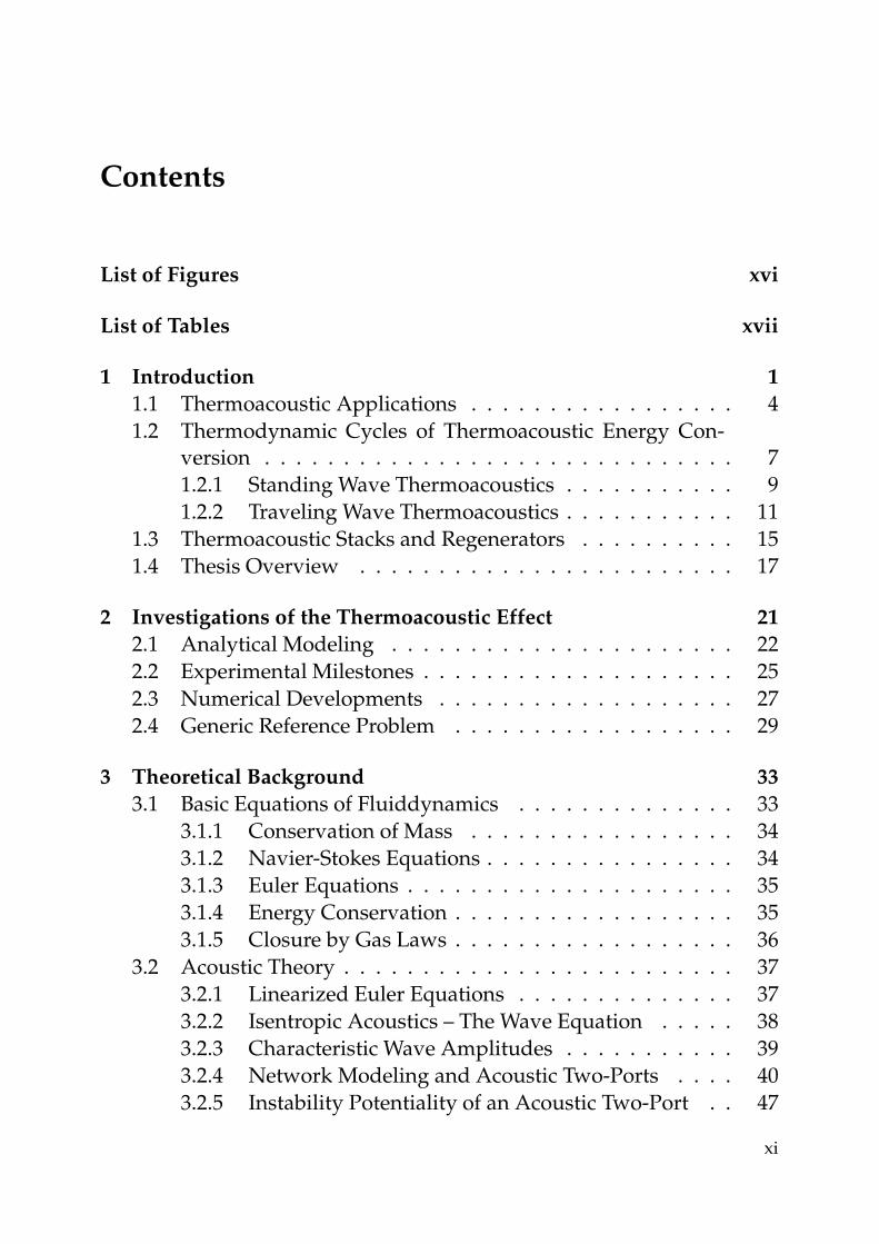
Contents
List of Figures xvi
List of Tables xvii
1 Introduction 1
1.1 Thermoacoustic Applications . . . . . . . . . . . . . . . . . 4
1.2 Thermodynamic Cycles of Thermoacoustic Energy Con-version . . . . . . . . . . . . . . . . . . . . . . . . . . . . . . 7
1.2.1 Standing Wave Thermoacoustics . . . . . . . . . . . 9
1.2.2 Traveling Wave Thermoacoustics . . . . . . . . . . . 11
1.3 Thermoacoustic Stacks and Regenerators . . . . . . . . . . 15
1.4 Thesis Overview . . . . . . . . . . . . . . . . . . . . . . . . 17
2 Investigations of the Thermoacoustic Effect 21
2.1 Analytical Modeling . . . . . . . . . . . . . . . . . . . . . . 22
2.2 Experimental Milestones . . . . . . . . . . . . . . . . . . . . 25
2.3 Numerical Developments . . . . . . . . . . . . . . . . . . . 27
2.4 Generic Reference Problem . . . . . . . . . . . . . . . . . . 29
3 Theoretical Background 33
3.1 Basic Equations of Fluiddynamics . . . . . . . . . . . . . . 33
3.1.1 Conservation of Mass . . . . . . . . . . . . . . . . . 34
3.1.2 Navier-Stokes Equations . . . . . . . . . . . . . . . . 34
3.1.3 Euler Equations . . . . . . . . . . . . . . . . . . . . . 35
3.1.4 Energy Conservation . . . . . . . . . . . . . . . . . . 35
3.1.5 Closure by Gas Laws . . . . . . . . . . . . . . . . . . 36
3.2 Acoustic Theory . . . . . . . . . . . . . . . . . . . . . . . . . 37
3.2.1 Linearized Euler Equations . . . . . . . . . . . . . . 37
3.2.2 Isentropic Acoustics – The Wave Equation . . . . . 38
3.2.3 Characteristic Wave Amplitudes . . . . . . . . . . . 39
3.2.4 Network Modeling and Acoustic Two-Ports . . . . 40
3.2.5 Instability Potentiality of an Acoustic Two-Port . . 47
xi
CONTENTS
3.2.6 Analytical Solutions Obtained by the Green’s Func-tion Method . . . . . . . . . . . . . . . . . . . . . . . 52
4 Inclusion of Mean Flow in Quasi 1D Thermoacoustic Transport
Equations 55
4.1 Dimensionless Two-Dimensional Navier-Stokes Equations 57
4.2 Asymptotic Expansion . . . . . . . . . . . . . . . . . . . . . 60
4.2.1 Narrow Pore and Linear Acoustics Assumption . . 65
4.3 Determination of Mean Field Quantities . . . . . . . . . . . 66
4.4 Linearized Navier-Stokes Equations . . . . . . . . . . . . . 69
4.5 One-Dimensional Thermoacoustic Transport . . . . . . . . 70
4.5.1 Simplification Approaches . . . . . . . . . . . . . . 71
4.5.2 Closure Assumptions . . . . . . . . . . . . . . . . . 72
4.5.3 Spatial Averaging of the TAPEs . . . . . . . . . . . . 74
4.5.4 Achieving High Modeling Accuracy . . . . . . . . . 79
4.6 Numerical Implementation of the TATEs . . . . . . . . . . 83
4.6.1 General Solution Technique . . . . . . . . . . . . . . 83
4.6.2 Implementation . . . . . . . . . . . . . . . . . . . . . 84
4.7 Advantages and Drawbacks of Mean Flow Inclusion . . . 84
5 CFD/SI - Time Domain Analysis of Thermoacoustic Scattering 87
5.1 System Identification . . . . . . . . . . . . . . . . . . . . . . 89
5.2 CFD Simulation . . . . . . . . . . . . . . . . . . . . . . . . . 92
5.2.1 Case Setup . . . . . . . . . . . . . . . . . . . . . . . . 93
5.2.2 Material Properties . . . . . . . . . . . . . . . . . . . 97
5.2.3 Boundary Conditions . . . . . . . . . . . . . . . . . 97
5.2.4 Initial Conditions . . . . . . . . . . . . . . . . . . . . 99
5.2.5 Post-Processing Methods and WHI Settings . . . . . 100
6 Experimental Determination of Thermoacoustic Effects 103
6.1 Multi Microphone Method . . . . . . . . . . . . . . . . . . . 104
6.1.1 Two Microphone Method and its Development . . 105
6.1.2 Multi Microphone Method in Non-Isentropic Con-ditions . . . . . . . . . . . . . . . . . . . . . . . . . . 106
6.1.3 Reconstruction from TA Core Data . . . . . . . . . . 111
6.2 Mode Shape, Onset and Limit Cycles of TA Engines . . . . 114
6.3 Experimental Setup . . . . . . . . . . . . . . . . . . . . . . . 115
xii
CONTENTS
6.3.1 TA Engine Setup . . . . . . . . . . . . . . . . . . . . 116
6.3.2 Multi-Microphone-Method Setup . . . . . . . . . . 120
6.3.3 Measurement Processs . . . . . . . . . . . . . . . . . 121
7 Thermoacoustic Interaction in Zero Mean Flow Conditions 125
7.1 Scattering Behavior of Thermoacoustic Stacks . . . . . . . . 125
7.1.1 One-Dimensional Models and CFD/SI Data . . . . 126
7.1.2 Analytical Limits . . . . . . . . . . . . . . . . . . . . 128
7.1.3 Comparison with Experimental Results . . . . . . . 131
7.1.4 Accuracy of Applied Methods . . . . . . . . . . . . 133
7.2 Thermoacoustic Engine Operation Mode . . . . . . . . . . 143
7.2.1 Mode shape of the First Eigenmode . . . . . . . . . 144
7.2.2 Thermoacoustic Onset . . . . . . . . . . . . . . . . . 147
7.2.3 Limit Cycle Oscillations . . . . . . . . . . . . . . . . 149
7.3 Instability Potentiality of TA Stacks and Regenerators . . . 151
7.3.1 Influence of Mean Parameters . . . . . . . . . . . . . 153
8 Impact of Mean Flow on the Scattering Behavior of TA Stacks 161
8.1 Experimental Mean Flow Results . . . . . . . . . . . . . . . 162
8.2 CFD/SI Mean Flow Results . . . . . . . . . . . . . . . . . . 164
8.3 1D-Modeling of Mean Flow Affected Regenerators . . . . . 166
8.3.1 Heat Conduction Dominated Conditions . . . . . . 166
8.3.2 Peclet Number Controlled Conditions . . . . . . . . 168
9 Conclusions and Outlook 171
Supervised Theses 175
References 179
A Details of the Derivation of the Quasi 1D-Model 201
A.1 Higher Order Terms in the Dimensionless NSEs . . . . . . 201
A.2 Abbreviations for the Analytical Approaches . . . . . . . . 202
A.2.1 Axial Momentum Equation . . . . . . . . . . . . . . 203
A.2.2 Energy Equation . . . . . . . . . . . . . . . . . . . . 203
A.2.3 Gas Law . . . . . . . . . . . . . . . . . . . . . . . . . 204
A.2.4 Conservation of Mass . . . . . . . . . . . . . . . . . 205
xiii

CONTENTS
B Experimental Modeling Approaches 207
B.1 Approximated Temperature Distribution Inside theDownstream Duct . . . . . . . . . . . . . . . . . . . . . . . . 207
B.2 Reconstructed Network Representations of the heaters . . 209
xiv
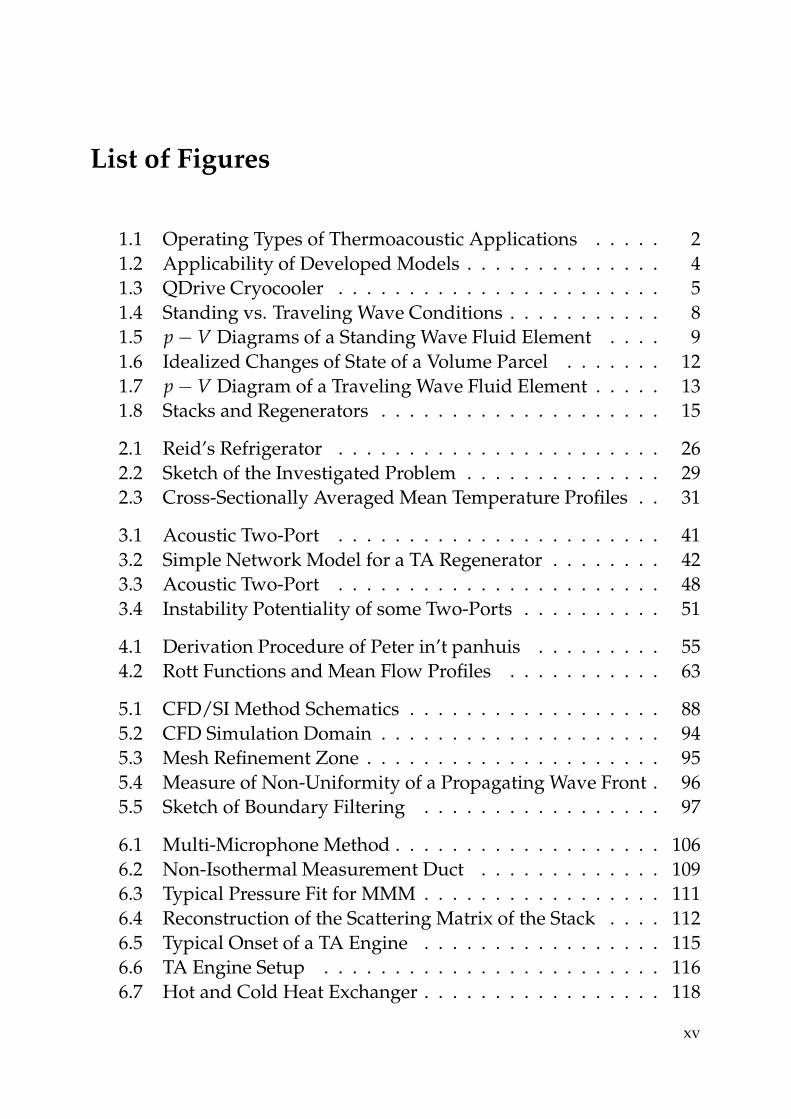
List of Figures
1.1 Operating Types of Thermoacoustic Applications . . . . . 2
1.2 Applicability of Developed Models . . . . . . . . . . . . . . 4
1.3 QDrive Cryocooler . . . . . . . . . . . . . . . . . . . . . . . 5
1.4 Standing vs. Traveling Wave Conditions . . . . . . . . . . . 8
1.5 p − V Diagrams of a Standing Wave Fluid Element . . . . 9
1.6 Idealized Changes of State of a Volume Parcel . . . . . . . 12
1.7 p − V Diagram of a Traveling Wave Fluid Element . . . . . 13
1.8 Stacks and Regenerators . . . . . . . . . . . . . . . . . . . . 15
2.1 Reid’s Refrigerator . . . . . . . . . . . . . . . . . . . . . . . 26
2.2 Sketch of the Investigated Problem . . . . . . . . . . . . . . 29
2.3 Cross-Sectionally Averaged Mean Temperature Profiles . . 31
3.1 Acoustic Two-Port . . . . . . . . . . . . . . . . . . . . . . . 41
3.2 Simple Network Model for a TA Regenerator . . . . . . . . 42
3.3 Acoustic Two-Port . . . . . . . . . . . . . . . . . . . . . . . 48
3.4 Instability Potentiality of some Two-Ports . . . . . . . . . . 51
4.1 Derivation Procedure of Peter in’t panhuis . . . . . . . . . 55
4.2 Rott Functions and Mean Flow Profiles . . . . . . . . . . . 63
5.1 CFD/SI Method Schematics . . . . . . . . . . . . . . . . . . 88
5.2 CFD Simulation Domain . . . . . . . . . . . . . . . . . . . . 94
5.3 Mesh Refinement Zone . . . . . . . . . . . . . . . . . . . . . 95
5.4 Measure of Non-Uniformity of a Propagating Wave Front . 96
5.5 Sketch of Boundary Filtering . . . . . . . . . . . . . . . . . 97
6.1 Multi-Microphone Method . . . . . . . . . . . . . . . . . . . 106
6.2 Non-Isothermal Measurement Duct . . . . . . . . . . . . . 109
6.3 Typical Pressure Fit for MMM . . . . . . . . . . . . . . . . . 111
6.4 Reconstruction of the Scattering Matrix of the Stack . . . . 112
6.5 Typical Onset of a TA Engine . . . . . . . . . . . . . . . . . 115
6.6 TA Engine Setup . . . . . . . . . . . . . . . . . . . . . . . . 116
6.7 Hot and Cold Heat Exchanger . . . . . . . . . . . . . . . . . 118
xv
6.8 Picture of the Regenerator . . . . . . . . . . . . . . . . . . . 119
6.9 Sketch of the MMM Setup . . . . . . . . . . . . . . . . . . . 121
7.1 Scattering Matrix from 1D-Models and CFD Data . . . . . 126
7.2 TA Scattering Matrix vs. Simple Limit Model . . . . . . . . 129
7.3 Experimental Data vs. Quasi 1D Data . . . . . . . . . . . . 131
7.4 Validation of tud . . . . . . . . . . . . . . . . . . . . . . . . . 135
7.5 Microphone Deviations from Fit Profile . . . . . . . . . . . 138
7.6 Maximum Experimental Errors . . . . . . . . . . . . . . . . 140
7.7 Standard Deviation of Measurements . . . . . . . . . . . . 141
7.8 Onset and Limit Cycle of TA Engine Setup . . . . . . . . . 144
7.9 Mode Shape of Engine Setup . . . . . . . . . . . . . . . . . 145
7.10 FFT of the TA Engine in its Limit Cycle . . . . . . . . . . . 150
7.11 Instability Potentiality of the Reference Case . . . . . . . . 151
7.12 Instability Potentiality for Different Shapes . . . . . . . . . 154
7.13 Prandtl Number Variations . . . . . . . . . . . . . . . . . . 156
7.14 IP of Different Pressurization Levels . . . . . . . . . . . . . 157
7.15 Mean Temperature Dependency of the IP . . . . . . . . . . 158
8.1 Experimental Mean Flow Scattering Matrices . . . . . . . . 162
8.2 Scattering Matrices Obtained by CFD/SI . . . . . . . . . . 164
8.3 1D-Models vs. CFD/SI for Pelin . . . . . . . . . . . . . . . . 167
8.4 1D-Models vs. CFD/SI for Peexp . . . . . . . . . . . . . . . 168
B.1 Temperature Fit for MMM . . . . . . . . . . . . . . . . . . . 208
B.2 Network Representation of the Ambient heater . . . . . . . 209
B.3 Experimental Data vs. Model Data of the Cold heater . . . 211
B.4 Network Representation of the Hot heater . . . . . . . . . . 212
List of Tables
4.1 Dimensionless Numbers of Narrow Pores . . . . . . . . . . 59
4.2 Overview of Mathematical Derivation Steps . . . . . . . . . 71
4.3 Overview Over the Modeled Terms . . . . . . . . . . . . . . 73
xvi

LIST OF TABLES
4.4 Replacement Characters and Their Indexing . . . . . . . . 75
B.1 Geometrical Parameters of the Ambient heater NetworkRepresentation . . . . . . . . . . . . . . . . . . . . . . . . . . 210
B.2 Geometrical Parameters of the Heater Network Represen-tation . . . . . . . . . . . . . . . . . . . . . . . . . . . . . . . 213
xvii

LIST OF TABLES
xviii
1 Introduction
Energy has been a perennial topic since the beginning of the industrialrevolution in the 18th century. From that time on its worldwide demandhas risen steadily. Today, especially emerging markets and developingcountries insist on a rising amount of resources for domestic and indus-trial use. This trend will lead to increasing environmental problems thathave to be faced. The industrial nations tackle this problem by forcingtheir industry to reduce their CO2 equivalent by self-dictated restrictions.Consequently, the interest in efficient energy conversion has been a cur-rent topic in research activity in the recent decades. Traditional energyconversion techniques have been exploited up to their efficiency limits.Hence, the investigation of less common methods becomes more andmore interesting for special applications like waste heat recovery or ef-ficient cooling.
Thermoacoustic (TA) boundary layer interaction causes energy conver-sion effects that can be exploited in both power generation and thermalmanagement. This type of energy conversion combines positive aspects,such as theoretical high efficiency and low maintenance costs because ofthe absence of moving parts and low minimum driving levels. Thesepromising issues have pushed the research activity in TAs over almostthree decades. They have yielded, among other innovations, analyticaldescriptions of the effect. However, the performance of the technologyachieved in practice is still far from the theoretical potential. Additionalresearch effort is needed to improve the applicability of this form of en-ergy conversion.
Existing analytical formalisms that describe this mechanism are basedon simplifications and hence do not account for several technically in-evitable effects. One of the most restricting assumptions is ignoring themean flow impact on acoustic transport inside TA regenerators. The goalof this study is to expand the understanding of the influence of meanflow on TA boundary layer interaction, focusing on the transmission and
1
1 Introduction
back scattering of acoustic waves in components experiencing such con-ditions. Analytical considerations yield a fast quasi one-dimensional pre-diction tool for future technical applications. This approach is validatedagainst numerical and experimental results obtained for a generic prob-lem.
The research field of thermoacoustics focuses on effects that originatefrom thermal and acoustic background. The most common topic is theinvestigation of the energy feedback between acoustics and heat releasein systems containing enclosed flames. Apart from this undesired ef-fect this thesis treats a research topic that handles a deliberate couplingof thermal and acoustic mechanisms. In modern literature this effect ismore and more referred to as “the thermoacoustic (TA) effect” [77, 115, 174],which causes a transformation from acoustic power into steady state heatflux in the vicinity of rigid walls or vice versa.
Refrigerator
Q
Q
W
Displacement x
Tem
per
atu
reT
δQ
δQParcelWall
(a)
Engine
Q
Q
W
Displacement x
Tem
per
atu
reT
δQ
δQWall
Parcel
(b)
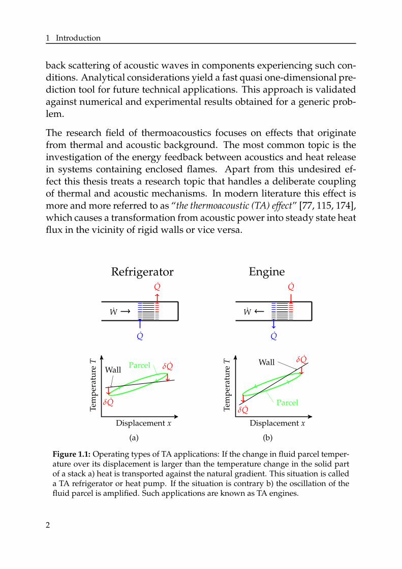
Figure 1.1: Operating types of TA applications: If the change in fluid parcel temper-ature over its displacement is larger than the temperature change in the solid partof a stack a) heat is transported against the natural gradient. This situation is calleda TA refrigerator or heat pump. If the situation is contrary b) the oscillation of thefluid parcel is amplified. Such applications are known as TA engines.
2
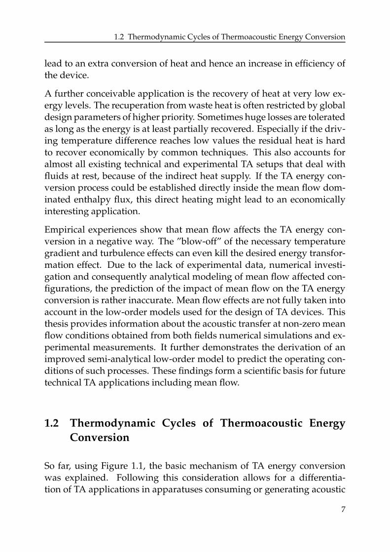
The most simple TA apparatus consists of a module of two heat exchang-ers adjacent to a porous media – so called stacks or regenerators – whichare located near the closed end of a wide duct. The two sketches dis-played in the top part of Figure 1.1 depict the energy transport for bothconfigurations. If heat Q is pumped from a cold region to a hot reservoir(Fig. 1.1a), acoustic power W has to be fed into the system. Depending onthe application, apparatuses employing this kind of energy conversionare distinguished as TA “refrigerators” or “heat pumps” [60]. If the TAenergy conversion process is reverted (Fig. 1.1b), a part of Q being trans-ported from the hot to the cold reservoir is converted into W. As acousticpower is generated, such systems are referred to as “TA engines” and“prime movers”.
An intuitive explanation of the TA effect can be given by an idealized con-sideration of a fluid volume parcel oscillating inside a part of the porousmedia, which for simplicity is modeled as a channel of constant height.Acoustic perturbations in gases at stagnant conditions usually lead to re-versible, isentropic changes of thermodynamic state. In wide ducts theadiabatic compression and expansion of a fluid parcel cause an oscilla-tory displacement in axial direction, which coincides with an acoustictemperature fluctuation T1. With decreasing duct diameter this fluctua-tion is affected by the local temperature of the solid wall. In the vicinityof the wall the temperature undergoes a cycle, which is sketched by thegreen ellipses in the lower part of Figure 1.1. When traveling towardslarger x-values, the compression due to the increasing acoustic pressurep1 causes an increase in T1. If the local temperature of the wall is lowerthan the actual fluid parcel value, heat is transfered to the wall, which isrejected when the parcel travels in negative x-direction. Hence the fluidtransports a certain amount of heat in the direction opposite to the axialtemperature gradient of the wall. Using parts of the acoustic power ofthe fluid, heat is pumped from a cold to a hot reservoir. This is shownin the top part of Figure 1.1a. The effect is reversed when the mean tem-perature gradient ∂T0/∂x is steeper than the gradient experienced by thefluid parcel. In the configuration displayed in Figure 1.1b a part of theheat flux is converted into acoustic power, which may lead to an acousticinstability.
3
1 Introduction
If mean flow affects the oscillation of the volume parcel, the thermody-namic cycle it undergoes is no more closed. As long as the displacementcaused by the mean velocity u0 is much smaller than the oscillatory coun-terpart, the system still performs at similar conditions. When u0 > u1 isreached not only the mean field conditions change, but also the changesof state cannot be described by the idealized consideration presentedabove. Furthermore, the analytical models which are derived for stag-nant mean flow conditions are no more valid. Thus these models have tobe adapted to non-zero mean flow conditions.
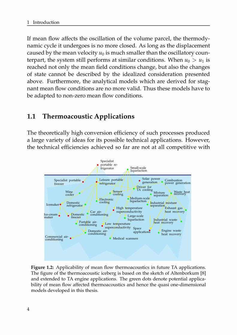
1.1 Thermoacoustic Applications
The theoretically high conversion efficiency of such processes produceda large variety of ideas for its possible technical applications. However,the technical efficiencies achieved so far are not at all competitive with
Leisure portablerefrigerator
Specialistportable re-frigerator
Specialist portablefreezer
Winecooler
IcemakerDomesticrefrigerator
Electroniccooling
Ice-creammaker
Domesticfreezer
Car air-conditioning
Portable air-conditioning
Domestic air-conditioning
Commercial air-conditioning
High temperaturesuperconductivity
Small-scaleliquefaction
Sensorcooling
Medium-scaleliquefaction
Low temperaturesuperconductivity
Medical scanners
Large-scaleliquefaction
Solar powergeneration
Combustionpower generation
Driver forTA cooling
Waste heatrecovery
Spaceapplications
Exhaust gasheat recovery
Industrial mixtureseparation
Industrial wasteheat recovery
Engine wasteheat recovery
Mixtureseparation
Figure 1.2: Applicability of mean flow thermoacoustics in future TA applications.The figure of the thermoacoustic iceberg is based on the sketch of Altenborkum [8]and extended to TA engine applications. The green dots denote potential applica-bility of mean flow affected thermoacoustics and hence the quasi one-dimensionalmodels developed in this thesis.
4
1.1 Thermoacoustic Applications
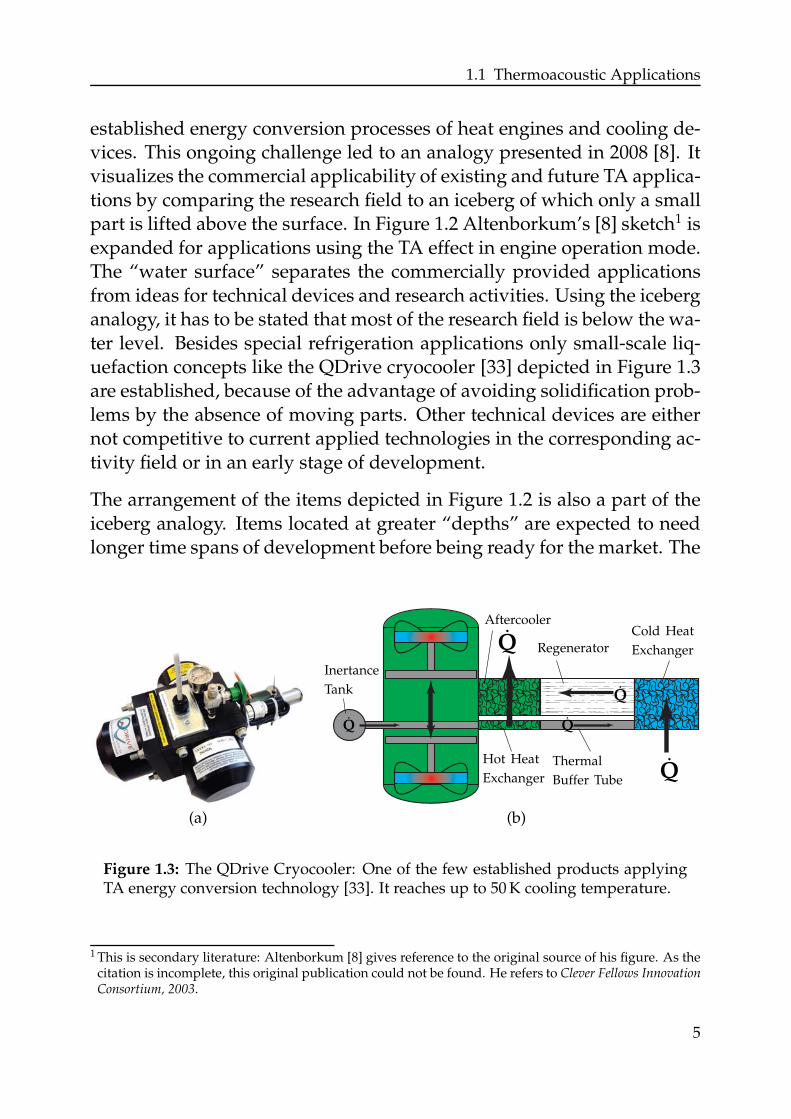
established energy conversion processes of heat engines and cooling de-vices. This ongoing challenge led to an analogy presented in 2008 [8]. Itvisualizes the commercial applicability of existing and future TA applica-tions by comparing the research field to an iceberg of which only a smallpart is lifted above the surface. In Figure 1.2 Altenborkum’s [8] sketch1 isexpanded for applications using the TA effect in engine operation mode.The “water surface” separates the commercially provided applicationsfrom ideas for technical devices and research activities. Using the iceberganalogy, it has to be stated that most of the research field is below the wa-ter level. Besides special refrigeration applications only small-scale liq-uefaction concepts like the QDrive cryocooler [33] depicted in Figure 1.3are established, because of the advantage of avoiding solidification prob-lems by the absence of moving parts. Other technical devices are eithernot competitive to current applied technologies in the corresponding ac-tivity field or in an early stage of development.
The arrangement of the items depicted in Figure 1.2 is also a part of theiceberg analogy. Items located at greater “depths” are expected to needlonger time spans of development before being ready for the market. The
800
(a) (b)
Inertance
Tank
Hot Heat
Exchanger
Thermal
Buffer Tube
Cold Heat
ExchangerRegenerator
Aftercooler
Q
Q
Q
Q
Q
Figure 1.3: The QDrive Cryocooler: One of the few established products applyingTA energy conversion technology [33]. It reaches up to 50 K cooling temperature.
1 This is secondary literature: Altenborkum [8] gives reference to the original source of his figure. As thecitation is incomplete, this original publication could not be found. He refers to Clever Fellows InnovationConsortium, 2003.
5
1 Introduction
yellow arrays give an idea of the evolution steps that have to be processedbefore certain devices could reach their break-through.
For example the generation of acoustic power from a biomass combustorwith the aim of developing a stove with a stand-alone source for electricalpower is an ongoing project [34, 119]. If the production costs per appara-tus are reduced by half, the project denoted as SCORE [162] is ripe for themarket. The same accounts for waste heat recovery systems which havealready been mounted as prototypes to small industrial applications [43].
On the bottom of the iceberg medical scanners are listed. The applicationof TA tomography [98] is an alternative to technologies using ultrasonicsound. Although the mathematical theory is fully provided [99], furtherresearch activity is needed to make this technology competitive to exist-ing technologies. Further as TA liquefaction plays a certain role in thistechnology, a stable medium-scale liquefaction should be established onthe market first. Therefore, TA tomography is far away from being usedcommercially.
The huge discrepancy between the number of commercially establishedand theoretically conceivable TA devices shows the long way TA researchstill has to go. The wide range of the applicability of the TA technologyprovides space for promising niche applications.
One area investigated only in a cursory manner is the application ofTA energy conversion in combination with mean flow. Existing ideasmainly focus on stagnant mean flow conditions. In many applicationsthe large oscillations at operating conditions cause undesired streamingeffects which limit the efficiency of many devices. Some of the topicslisted in Figure 1.2 are related to mean flow effects. The green dots in-dicate fields of research where non-stagnant conditions may either occuror can even be used beneficially. TA mixture separation only works ifthe products can be transported towards the separation device. Thus acertain mean flow inside such applications occurs necessarily. Car air-conditioning and exhaust gas heat recovery are also linked to convectiondominated energy flux. Under certain circumstances, a direct couplingof the gas stream with TA energy conversion in the latter example may
6
1.2 Thermodynamic Cycles of Thermoacoustic Energy Conversion
lead to an extra conversion of heat and hence an increase in efficiency ofthe device.
A further conceivable application is the recovery of heat at very low ex-ergy levels. The recuperation from waste heat is often restricted by globaldesign parameters of higher priority. Sometimes huge losses are toleratedas long as the energy is at least partially recovered. Especially if the driv-ing temperature difference reaches low values the residual heat is hardto recover economically by common techniques. This also accounts foralmost all existing technical and experimental TA setups that deal withfluids at rest, because of the indirect heat supply. If the TA energy con-version process could be established directly inside the mean flow dom-inated enthalpy flux, this direct heating might lead to an economicallyinteresting application.
Empirical experiences show that mean flow affects the TA energy con-version in a negative way. The ”blow-off” of the necessary temperaturegradient and turbulence effects can even kill the desired energy transfor-mation effect. Due to the lack of experimental data, numerical investi-gation and consequently analytical modeling of mean flow affected con-figurations, the prediction of the impact of mean flow on the TA energyconversion is rather inaccurate. Mean flow effects are not fully taken intoaccount in the low-order models used for the design of TA devices. Thisthesis provides information about the acoustic transfer at non-zero meanflow conditions obtained from both fields numerical simulations and ex-perimental measurements. It further demonstrates the derivation of animproved semi-analytical low-order model to predict the operating con-ditions of such processes. These findings form a scientific basis for futuretechnical TA applications including mean flow.
1.2 Thermodynamic Cycles of Thermoacoustic Energy
Conversion
So far, using Figure 1.1, the basic mechanism of TA energy conversionwas explained. Following this consideration allows for a differentia-tion of TA applications in apparatuses consuming or generating acoustic
7
1 Introduction
|u1|,|p
1|
(a)
|u1|,|p
1|
(b)
x x
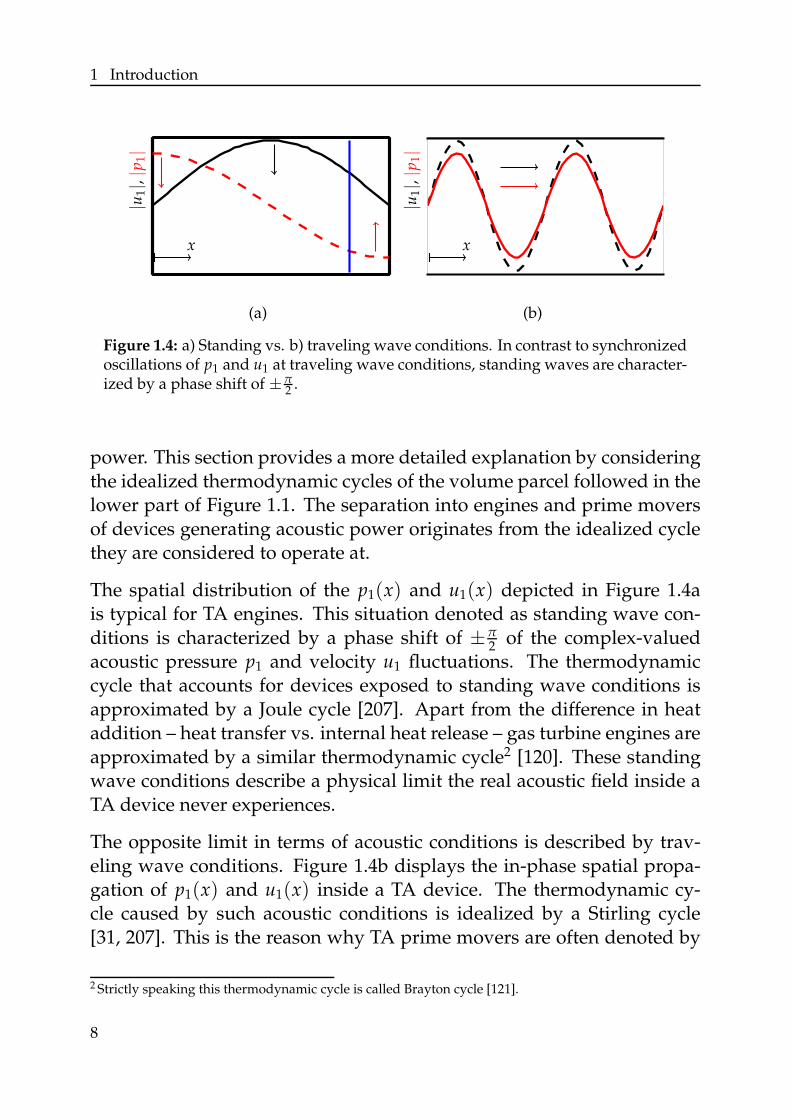
Figure 1.4: a) Standing vs. b) traveling wave conditions. In contrast to synchronizedoscillations of p1 and u1 at traveling wave conditions, standing waves are character-ized by a phase shift of ±π
2 .
power. This section provides a more detailed explanation by consideringthe idealized thermodynamic cycles of the volume parcel followed in thelower part of Figure 1.1. The separation into engines and prime moversof devices generating acoustic power originates from the idealized cyclethey are considered to operate at.
The spatial distribution of the p1(x) and u1(x) depicted in Figure 1.4ais typical for TA engines. This situation denoted as standing wave con-ditions is characterized by a phase shift of ±π
2 of the complex-valuedacoustic pressure p1 and velocity u1 fluctuations. The thermodynamiccycle that accounts for devices exposed to standing wave conditions isapproximated by a Joule cycle [207]. Apart from the difference in heataddition – heat transfer vs. internal heat release – gas turbine engines areapproximated by a similar thermodynamic cycle2 [120]. These standingwave conditions describe a physical limit the real acoustic field inside aTA device never experiences.
The opposite limit in terms of acoustic conditions is described by trav-eling wave conditions. Figure 1.4b displays the in-phase spatial propa-gation of p1(x) and u1(x) inside a TA device. The thermodynamic cy-cle caused by such acoustic conditions is idealized by a Stirling cycle[31, 207]. This is the reason why TA prime movers are often denoted by
2 Strictly speaking this thermodynamic cycle is called Brayton cycle [121].
8
1.2 Thermodynamic Cycles of Thermoacoustic Energy Conversion
TA Stirling engines. Sometimes such devices are also called “travelingwave engines”.
Neither of these two operating conditions are reached in TA applications.As they form the limit conditions an oscillating which a volume parcelexperiences, investigating it under these two idealized conditions leadsto a deeper qualitative insight to TA energy conversion. In the next twosections we follow such a parcel located in the region marked by the blueline in Figure 1.4 for both limit conditions. In order to make the investi-gation more intuitive, the changes of displacement, acoustic pressure p1
and acoustic velocity u1 of the parcel are idealized by square wave sig-nals. Here we focus on acoustic power generation, i.e. TA engine andheat pump applications. The same ideas can be applied to the consid-eration of acoustic power consumption. If so, the inverse temperaturedifferences to the wall cause a change in the direction of the fluxes ofheat and power.
1.2.1 Standing Wave Thermoacoustics
Volume V
Pre
ssu
rep
s
y ≫ δK
(a)
Volume V
Pre
ssu
rep
T
y ≪ δK
(b)
Volume V
Pre
ssu
rep
p
pG
A
s
B
D
s
Cy ∼ δK
(c)
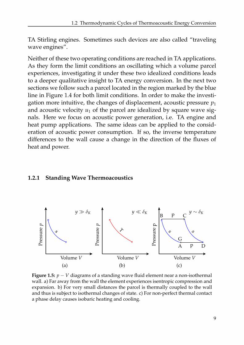
Figure 1.5: p − V diagrams of a standing wave fluid element near a non-isothermalwall. a) Far away from the wall the element experiences isentropic compression andexpansion. b) For very small distances the parcel is thermally coupled to the walland thus is subject to isothermal changes of state. c) For non-perfect thermal contacta phase delay causes isobaric heating and cooling.
9

1 Introduction
As shown in the introduction, the interaction between the fluid and thesolid wall is crucial for TA energy conversion. The length scales charac-terizing this problem are the viscous acoustic penetration depth
δν =
√
2ν
ω(1.1)
and thermal acoustic penetration depth
δK =
√
2K
ωcp0. (1.2)
Both quantities scale with the inverse square root of angular frequencyω and the material properties of the fluid. The viscous acoustic penetra-tion depth δν depends on the kinematic viscosity ν. The fraction of ther-mal conductivity K and the product of specific capacity of heat cp andmean density 0 is denoted as thermal diffusivity and forms the equiv-alent for the thermal penetration depth δK. Here, we consider the ratioof the distance y between the volume parcel and the wall to the ther-mal penetration depth δK as the measure allowing for a classification intothree different situations:
y ≫ δK: General acoustics deals with parcels that are not affected by thewall. Due to the poor contact to the wall, the isentropic changeof state of the parcel is not affected by the solid temperature. Theblue line(s) in the p − v diagram presented in Figure 1.5a depictsall acoustic states such a parcel experiences. As no area is enclosedby the changes of state, acoustic energy is neither consumed norgenerated.
y ≪ δK: The fluid parcel is in perfect thermal contact to the wall. Hence,the compression it experiences when being displaced towardshigher acoustic pressure at larger x-values leads to a simultane-ous heating. The hotter solid wall passes heat to the fluid parcelat lower temperature. When the parcel travels in the opposite di-rection, it is cooled while it expands to the lower acoustic pressureat its original position. Figure 1.5a displays the thermodynamicstates of such a parcel in terms of a red line (T). Again, they forma line which is insufficient for energy conversion. Like parcels the
10
1.2 Thermodynamic Cycles of Thermoacoustic Energy Conversion
first situation, this change of state is not restricted to the regionnear the blue line depicted in Figure 1.4a.
y ≈ δK: The thermal contact of the fluid volume to the correspondingwall location is imperfect. This causes a time delay between the ex-pansion/compression and the addition/subtraction of heat by thesolid wall. If a parcel located right of the blue line in Figure 1.4a isexposed to a positive axial mean temperature gradient, the pres-sure fluctuation is larger than the velocity counterpart. This leadsto small but non-negligible axial movements of the parcel thatare in phase with the pressure oscillation. During one oscilla-tion period it experiences a four step process that is displayed inFigure 1.5. Additionally the location, volume and temperature ofthe parcel is visualized in the left column of Figure 1.6:
1. The parcel is compressed (A → B) while being displaced to-wards higher pressure.
2. If acoustic power is generated, the hot wall at this locationheats (δQ1 > 0) the parcel (B → C). In addition the change involume does work at the system (δW1 < 0).
3. Next, the parcel expands while being displaced towards itsoriginal position (C → D).
4. Finally it is cooled (D → A) to its original state (δQ1 < 0)while work is freed δW2 < 0.
This thermodynamic cycle is known as Joule cycle [207]. As the imperfectthermal contact is crucial for the energy conversion process, TA devicesoperating with this cycle use porous media with hydraulic radii R largerthan the thermal penetration depth δK.
1.2.2 Traveling Wave Thermoacoustics
The characteristic thermodynamic cycle a traveling wave engines is op-erating with is shown in Figure 1.7. Additionally the parcel with perfectthermal wall contact δK ≪ y is sketched on the right column of Figure 1.6.In contrast to the phase shift of π/2 between acoustic pressure and veloc-ity in a standing wave application, the acoustic variables oscillate simul-
11
1 Introduction
Wave EngineWave EngineStanding Traveling
1. Compression
2. Heating
3. Expansion
4. Cooling
δQ1 δQ1
δQ2 δQ2
δW1
δW1
δW2
δW2
A → B
B → C
C → D
D → A
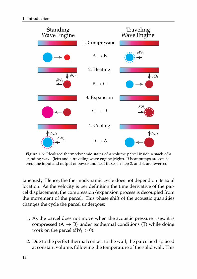
Figure 1.6: Idealized thermodynamic states of a volume parcel inside a stack of astanding wave (left) and a traveling wave engine (right). If heat pumps are consid-ered, the input and output of power and heat fluxes in step 2. and 4. are reversed.
taneously. Hence, the thermodynamic cycle does not depend on its axiallocation. As the velocity is per definition the time derivative of the par-cel displacement, the compression/expansion process is decoupled fromthe movement of the parcel. This phase shift of the acoustic quantitieschanges the cycle the parcel undergoes:
1. As the parcel does not move when the acoustic pressure rises, it iscompressed (A → B) under isothermal conditions (T) while doingwork on the parcel (δW1 > 0).
2. Due to the perfect thermal contact to the wall, the parcel is displacedat constant volume, following the temperature of the solid wall. This
12
1.2 Thermodynamic Cycles of Thermoacoustic Energy Conversion
isochoric change of state causes an input of heat (δQ1 > 0) into theparcel.
3. In the maximum positive deflection, the parcel expands (C → D)keeping the temperature of the wall. Mechanic power (δW2 < 0) isfreed by the fluid volume.
4. When it travels back to the negative point of deflection (D → A)leads to a heat release (δQ1 < 0) into the wall.
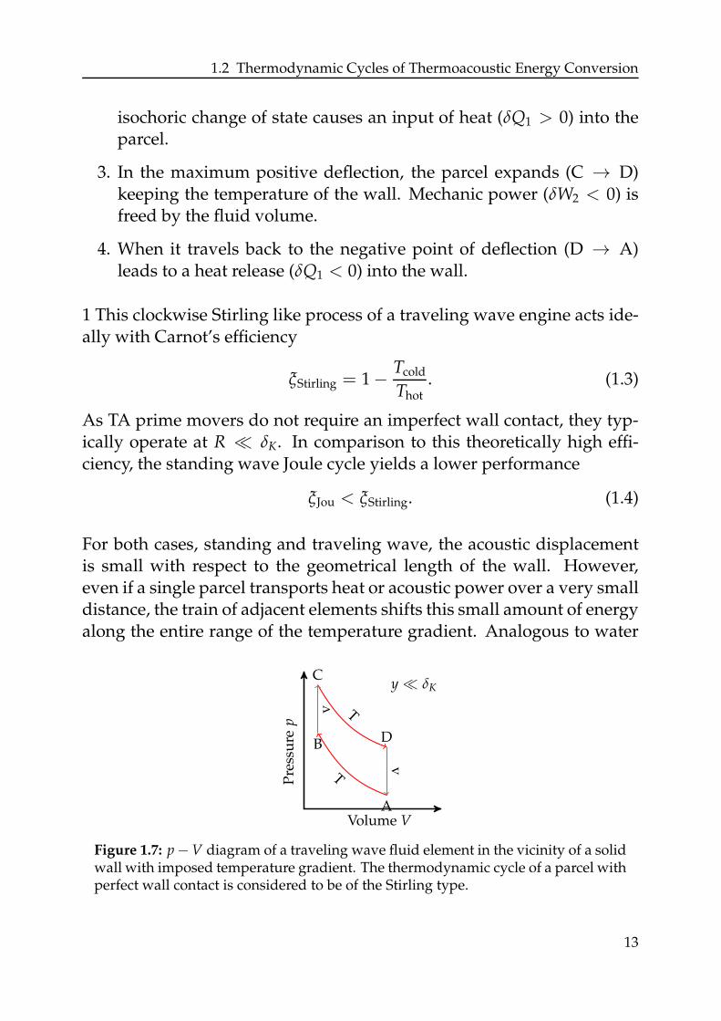
1 This clockwise Stirling like process of a traveling wave engine acts ide-ally with Carnot’s efficiency
ξStirling = 1 − Tcold
Thot. (1.3)
As TA prime movers do not require an imperfect wall contact, they typ-ically operate at R ≪ δK. In comparison to this theoretically high effi-ciency, the standing wave Joule cycle yields a lower performance
ξJou < ξStirling. (1.4)
For both cases, standing and traveling wave, the acoustic displacementis small with respect to the geometrical length of the wall. However,even if a single parcel transports heat or acoustic power over a very smalldistance, the train of adjacent elements shifts this small amount of energyalong the entire range of the temperature gradient. Analogous to water
Volume V
Pre
ssu
rep
C
T
D
v
A
T
B
v
y ≪ δK
Figure 1.7: p −V diagram of a traveling wave fluid element in the vicinity of a solidwall with imposed temperature gradient. The thermodynamic cycle of a parcel withperfect wall contact is considered to be of the Stirling type.
13
1 Introduction
buckets being passed from person to person to bridge the distance froma well to the scene of fire, this effect is referred to as bucket-brigading.
These idealized considerations are only valid for stagnant flow condi-tions. As soon as mean flow is present, the fluid parcel does not returnto the initial condition after one loop. In his Ph. D. thesis [158], Reidprovides an improved idealized condition for moderate mean flow con-dition. If the mean velocity increases to small values, the original ellipsesin Figure 1.1 degenerate toward spirals that propagate along the meanflow gradient. Only as long as the mean velocity u0 is that low, it affectsthe mean flow field and does not interfere directly with acoustic propaga-tion. While isobaric heat exchange in the standing wave cycle seems to bequite unaffected by this effect, the expansion and compression process inthe traveling wave configuration are no longer isothermal. Therefore, thethermodynamic cycle of the latter is expected to be affected more stronglyby mean flow effects.
Using the model of Reid, the impact of mean flow is accounted for bysolving a convection/diffusion equation for the cross-sectionally aver-aged mean flow temperature 〈T0〉(x). A solution for such a problem withconstant material properties has an exponential shape. With increasingPeclet number Pe of the mean flow field, the narrow geometry consistsof a larger region at approximately uniform temperature. Here, the ther-moacoustic energy conversion is clearly in the heat pumping regime. Therest of the duct is dominated by large mean temperature gradients. Asthese gradients ∂T0(x)/∂x lead to higher acoustic power production, thispart annihilates at least a part of the first conversion from power to heat.The integral impact of this combination on the acoustic propagation hasnot been investigated so far.
In technical applications the temperature profile is not fixed by boundaryconditions of the first kind. Thus using similar heat exchangers, parts ofthe steep profile are shifted inside the heat exchanger and do not causeTA interaction. Furthermore, mean flow leads to the formation of shearlayers. They especially form at the in- and outlet of the duct and arenot accounted for in the scope of this thesis. These shear layers inter-act with acoustic propagation in a dissipative way. The impact of meanflow inside the duct is partially accounted for in later investigations in
14
1.3 Thermoacoustic Stacks and Regenerators
this thesis. It will be shown that the transversal mean velocity profileplays a minor role for the acoustic propagation in the cases. Summariz-ing the ideas of possible mean flow impact on TA energy conversion, nobenefiting effect can be identified. Technical applications also could notgenerate conditions that improve the basic mechanism. Wherever meanflow occurs, the efficiency of the device is reduced.
1.3 Thermoacoustic Stacks and Regenerators
The simplified explanation of the TA energy conversion presented in thelast sections reveals the main requirement for the technical segment ofTA energy conversion. Both traveling and standing wave conversion cy-
300
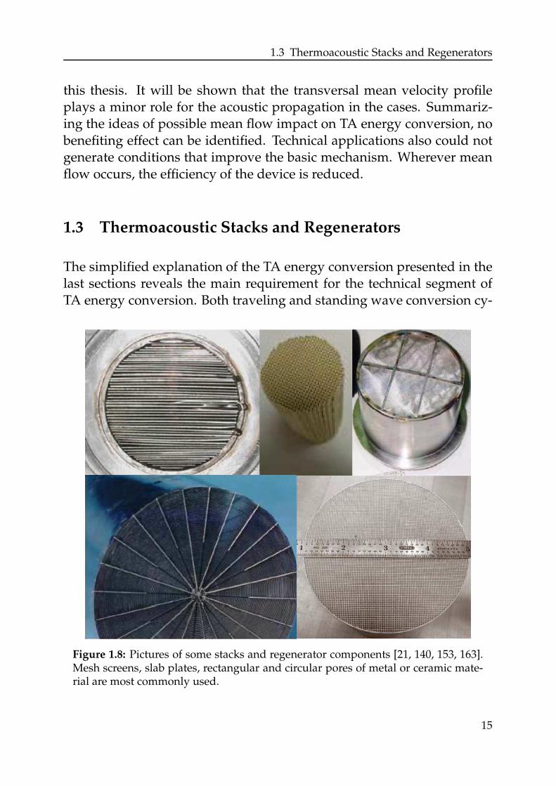
Figure 1.8: Pictures of some stacks and regenerator components [21, 140, 153, 163].Mesh screens, slab plates, rectangular and circular pores of metal or ceramic mate-rial are most commonly used.
15
1 Introduction
cles are characterized by the thermal acoustic boundary layer thickness.The hydraulic radius R of the selected component has to be at least ofa similar order of magnitude as δK. As this geometric restriction leadsto small amounts of power per pore, an efficient application of the effectimplies a parallel utilization of such components. A wide variety of ma-terials and forms were proposed by different authors; some are shownin Figure 1.8. Thermally low charged devices often operate with bun-dles of plastic pipes or packages of equally spaced plates [16]. Most ofthe applications use a slab-shaped pore geometry or other simple shapessuch as bundles of circular [184] or rectangular pipes [158]. Besides theseregular shaped geometries, arbitrary porous media with similar averagepore diameters also support the TA effect and can even be modeled ana-lytically [105]. Due to their wider thermal stability, copper [71], stainlesssteel [15] or ceramic based [212] devices are utilized in applications withhigh temperature differences. As long as the Lautrec number
La =Rh
δK, (1.5)
i.e. the ratio of hydraulic to acoustic length scale, is of the order of unityor smaller, the pore shape can be chosen arbitrarily. For example, steelwool [2] and even rice [129] were used for the energy conversion.
TA standing wave devices typically operate with porous media with1 < La < 10. In the literature they are denoted as stacks, as their firstprototypes consisted of stacks of parallel plates. As explained in the pre-vious section, the fluid outside the thermal boundary layer of travelingwave applications does not contribute to the energy conversion. There-fore a Lautrec number of La < 1 is required for this operation mode. Theidealized Stirling cycle suggests a direct comparison to the homonymoustype piston engines. Thus, the heat conversion unit is called regenerator.Nevertheless these various denominations describe the same componentand, depending on the operating frequency and the acoustic state, evenidentical components are referred to by different wordings. In this workthe acoustic scattering behavior of these components is investigated. Thismeans the transmitted and back scattered components are related to theincident acoustic waves. In general this is a frequency dependent prob-lem. As this thesis does not distinguish frequency ranges, regeneratorand stack are used as synonyms here.
16
1.4 Thesis Overview
1.4 Thesis Overview
The knowledge about thermoacoustic energy conversion in mean flow af-fected pores, investigated only fleetingly so far, is improved by providingdata sets and analytical prediction tools for this combination. The con-version performance of mean flow affected devices in all hitherto inves-tigated configurations always decreased with increasing Mach number.High Peclet numbers Pe cause an reduction of the axial temperature gra-dient inside the regenerators. The change in mean temperature is shiftedtowards the heat exchanger. No driving mean temperature gradient inthe pore establishes and the TA energy conversion breaks down. Highpore Reynolds numbers Re lead to turbulent perturbations and there-with distortion or deterioration of both acoustic boundary layers. Thus,researchers with the focus on constructing high efficient devices, whichare particularly based on TA energy conversion, always concentrate onsuppressing turbulent effects. Designing economically reasonable appli-cations operating in this regime requires a detailed knowledge of the in-teraction of the TA effect and non-stagnant mean conditions. Improvingthis understanding demands a universal approach. Thus, the thesis isstructured in an analytical, numerical and experimental investigation ofone generic reference configuration.
Chapter 2 briefly reviews the literature published on TA boundary layerinteraction. Starting from its discovery, the analytical, numerical and ex-perimental developments are presented. It focuses on publications whicheither contribute to the general understanding of TAs or provide infor-mation on mean flow affected devices. The problem considered in thisthesis is presented based on the investigation techniques applied.
The investigations processed in the main part of this thesis demand sometheoretical background. These include the basics of fluid dynamics, ther-modynamics and acoustics. Their fundamental equations are providedin Chapter 3. The theory of the latter topic is treated in detail. The de-scription of technical components in terms of acoustic multi-ports, theirtransmission behavior and instability potentiality (IP), a newly derivedacoustic power balance criterion, is explained by simple configurations.The chapter finally presents the derivation of a Green’s function (GF) for
17
1 Introduction
a form of ordinary differential equation that is encountered in subsequentchapters.
The interaction of thermoacoustic energy conversion and mean flow istreated theoretically in Chapter 4. The scope of this chapter is to providea quasi one-dimensional set of differential equations that describe suchconfigurations with higher accuracy than previous methods. The new ap-proach extends the formulation found by Peter in’t panhuis [82] using thesame derivation strategy. At first, the fluid transport equations account-ing for viscous friction and thermal diffusion are non-dimensionalizedusing characteristic parameters from boundary layer theory. In a sec-ond step the resulting equations experience a series expansion in termsof acoustic Mach number. The first order set of equations is simplifiedby assuming this quantity to be of the order of the ratio of dimensionsof the pore considered. Applying the method of separation of variablesto these equations, the GF presented in Chapter 3 allows for an analyti-cal solution for the transversal components of the acoustic quantities. Thecross-sectionally averaged3 form of the set of equations strongly dependson two closure assumptions that have to be found during the derivation.For the purpose of keeping the resulting system of equations short, twodifferent approaches are selected. These final equations are implementedin a numerical tool, which is later used to compute linear scattering ma-trices for given mean field configurations of the TA stack. The descriptionof the implementation is followed by a discussion of closure assumptionsof higher complexity.
For validating the scattering matrix results of the one-dimensional tool, amulti-dimensional numerical approach is carried out in Chapter 5. Com-putational fluid dynamics (CFD) is used to describe the TAs inside regen-erators affected by mean flow. The accuracy of CFD simulations scaleswith the precision of the geometric model and the exactness of resolutionof the dominating effects. Consequently, resolving all scales dominat-ing the problem leads to a highly accurate prediction of the flow fieldinside the domain. As CFD is hosted in the time domain, system iden-tification (SI) methods are needed for post processing. The theory of the
3 The application of the words “mean” and “average” are strictly distinguished: All parameters denotedas mean parameters are constant in time, while averaging refers to computed spatial (mostly cross-sectional) averaging of a quantity.
18
1.4 Thesis Overview
technique used in this work is laid out in Section 5.1. Using this so-calledCFD/SI method, the scattering behavior in the observed frequency rangecan be predicted in a single simulation run. The results of this methodenable a direct validation of the scattering matrices predicted by the one-dimensional tool.
Numerical and semi-analytical results are always based on modeling as-sumptions. In general only experimental results are assumed to be validwithin the accuracy of measurement errors. For this purpose an experi-mental test rig was set up for generating reference data. In Chapter 6 itssetup components and the measurement techniques applied are demon-strated. The multi-microphone technique, an improvement of the two-source location method of Munjal and Doige [123], delivers the acousticscattering behavior for the thermoacoustic core, a regenerator flanked bytwo heat exchangers. The use of recursive methods allows the determi-nation of the acoustic scattering matrices of the TA stack.
Chapter 7 discusses the predicted acoustic scattering behavior of thegeneric stack for stagnant mean flow conditions. The chapter considersthe acoustic scattering predicted by all three approaches. The frequencydependent scattering matrix values are further compared against a net-work model that approaches a stack pore by two viscous ducts enclosinga discrete temperature change. This simple model matches the scatteringbehavior in the high frequency regime. Whenever the thermoacousticenergy conversion is active, it deviates from the real matrix values andhence provides an insight into the impact of the TA effect to the scatter-ing behavior of the stack. An implementation of the computed scatteringmatrices into a network stability analysis tool facilitates a comparisonwith experimentally investigated TA engine operating conditions. Themodeled growth rate as well as the mode shape are investigated. Finallya parameter variation yields information about an optimum stack con-figuration in terms of IP. Applying this criterion facilitates the determi-nation of the limit amplification or attenuation of the observed acoustictwo-port.
The impact of mean flow on the acoustic scattering behavior is discussedin Chapter 8. The good qualitative agreement of the experimental andCFD/SI data forms a base for validation of the one-dimensional predic-
19
1 Introduction
tion models. The improvements of the newly derived over their prede-cessors are demonstrated. The chapter finally discusses the influence ofdifferent closure assumptions.
The thesis concludes with a brief outlook on the applicability of TA de-vices affected by mean flow and their importance is classified in the fieldof thermoacoustics.
20
2 Investigations of the Thermoacoustic Effect
The discovery of thermoacoustics dates back more than 200 years. Thereport of Higgins [69] on “singing flames“gave birth to TA research.He observed the occurrence of unstable acoustic modes when hydrogenflames were located in certain regions in open pipes. Rijke [161] replacedthe flames by a wire framed mesh and showed that in this case the TAphenomenon is linked to convection dominated energy conversion pro-cesses. Although Sondhauss [182] is considered to be the first investi-gator of spontaneous acoustic sounds emitted during the glass blowingprocess, Pinaud [139] and Carl Marx [112] tried to capture its physics tosome extent. Their publications even refer to investigations carried out atthe beginning of the 18th century, which mainly focus on musical aspectsof the construction of a thermal organ pipe. While Pinaud related thespontaneous loud emission of tones to local condensation phenomena,Marx, discovered a certain dependency on the glass pipe diameter andthe location of heating. In contrast to his predecessors, Sondhauss [182]was the first to provide technical data. Moreover, he investigated a corre-lation of the axial temperature gradient with the observed sound levels.This publication led to an immense amount of publications over the lasttwo centuries. They approach the problem of understanding these mech-anisms from three different directions. The experimental observationspublished for various configurations provide the data to validate the in-vestigations carried out with numerical simulations. The third type ofpublications provides simplified analytical models that lead to a betterunderstanding of the basic mechanisms. The literature referenced hereis also presented in three parts. At first, the history of analytical mod-eling is reviewed. The second section treats the most important experi-mental contributions, before Section 2.3 gives a brief overview over themilestones achieved by numerical simulations of the thermoacoustic ef-fect. For detailed information the reader is referred to review articles[25, 52, 53], the resource letter of Garrett [60], the book of Swift [187] andthe literature discussed therein.
21
2 Investigations of the Thermoacoustic Effect
Finally, Section 2.4 discusses the generic reference setup, which is usedfor the existing one-dimensional analytical models as well as for the newmodel developed in Chapter 4.
2.1 Analytical Modeling
Rayleigh [157] himself claimed that his general criterion for the occur-rence of any TA oscillation – an in-phase oscillation of pressure and heatrelease fluctuation – is fulfilled for the process described by Sondhauss[182], because “(...) the adjustment of air takes time, and thus the temperature(...) deviates from that of neighbouring parts. (...) From this it follows, that atthe phase of greatest condensation heat is received by the air, and at the phase ofgreatest rarefaction, heat is given up from it, and thus there is the tendency tomaintain the vibrations.“ However, he provided no analytical descriptionfor this phenomenon. Kirchhoff [92] was the first to consider the impactof thermal diffusion on acoustic propagation. He found that like vis-cous friction, this damping mechanism affects the propagation of acous-tic waves in terms of shifting the wave number from the real axis into thecomplex plane. Almost one century later Kramers [96] published a pro-found mathematical model to describe thermally damped and driven os-cillations in terms of acoustic pressure p1 and cross-sectionally averagedvelocity 〈u1〉. Like his predecessor, he considered an idealized pipe. Hisapproach was the first attempt to completely describe thermo-viscousboundary layer interaction, but he could not explain the acoustic am-plification in the presence of mean temperature gradients ∂T0/∂x. A fewyears later, Clement and Gaffner [37] derived a similar model, which wasbased on observed oscillations in cryogenic devices.
In the following decades, Merkli and Thomann [115] and especially Rottrefined Kramers model in a series of publications [164–171]. Using themethod of separation of variables, he found analytical solutions hν(y)for the transversal (y-dependent) profile of the acoustic velocity u1 inthe linearized axial momentum equation including viscous frictions andhK(y) of the temperature fluctuation T1 in the energy transport equationincluding thermal diffusion. For the description of circular pipes, heincorporated these solutions into the one-dimensional ODEs describing
22
2.1 Analytical Modeling
the axial acoustic propagation of p1 and the transversally averaged formof the acoustic velocity 〈u1〉. Furthermore, the second-order analysis ofenthalpy flux revealed a correlation of the mean temperature distribu-tion to acoustic quantities. Applying a harmonic ansatz, his observationsyielded a system of ordinary differential equations (ODEs) in frequencydomain. These ODEs are formulated in terms of acoustic pressure p1,transversally averaged velocity oscillation 〈u1〉, mean parameters andtwo functions fν,K = 〈hν,K〉 accounting for the cross-sectionally averagedimpact of viscous friction (index ν) and thermal diffusion (index K).
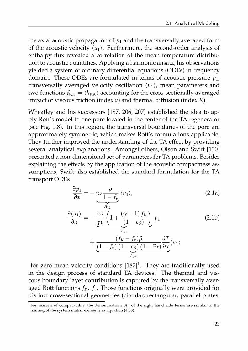
Wheatley and his successors [187, 206, 207] established the idea to ap-ply Rott’s model to one pore located in the center of the TA regenerator(see Fig. 1.8). In this region, the transversal boundaries of the pore areapproximately symmetric, which makes Rott’s formulations applicable.They further improved the understanding of the TA effect by providingseveral analytical explanations. Amongst others, Olson and Swift [130]presented a non-dimensional set of parameters for TA problems. Besidesexplaining the effects by the application of the acoustic compactness as-sumptions, Swift also established the standard formulation for the TAtransport ODEs
∂p1
∂x=− iω
ρ
1 − fν︸ ︷︷ ︸
A12
〈u1〉, (2.1a)
∂〈u1〉∂x
=− iω
γp
(
1 +(γ − 1) fK
(1 − ǫS)
)
︸ ︷︷ ︸
A21
p1 (2.1b)
+( fK − fν)β
(1 − fν) (1 − ǫS) (1 − Pr)
∂T
∂x︸ ︷︷ ︸
A22
〈u1〉
for zero mean velocity conditions [187]1. They are traditionally usedin the design process of standard TA devices. The thermal and vis-cous boundary layer contribution is captured by the transversally aver-aged Rott functions fK, fν. Those functions originally were provided fordistinct cross-sectional geometries (circular, rectangular, parallel plates,
1 For reasons of comparability, the denominations Aij of the right hand side terms are similar to thenaming of the system matrix elements in Equation (4.63).
23
2 Investigations of the Thermoacoustic Effect
etc.), before Arnott et al. [9] derived a general solution for these quanti-ties for arbitrarily shaped cross-sections. The system of Equations (2.1)includes the contribution of viscous dissipation as well as thermal dif-fusivity and the TA interaction. The viscous dissipation is taken intoaccount by the viscous Rott function fν in A12 of the acoustic pressuretransport Equation (2.1a) originating from the linearized axial momen-tum equation. Thermal diffusivity scales the energy transport (Eq. (2.1b))in terms of p1 and the thermal Rott function fK in A21. The third term A22
is controlled by a combination of the Rott functions. The compressibil-ity β and the mean temperature gradient also affect the TA interaction.The influence of thermal oscillations inside the solid region was addedby Swift’s student Ward [189] using the scaling parameter ǫS, a productof the ratio of thermal diffusivities and geometrical functions.
The attempt of Reid and Swift [159] to take mean flow into account has al-ready been introduced in Section 1.2.2. They considered the mean veloc-ity to be of second order. Thus terms containing u0 do not appear in thelinearized system of equations. To account for the changes in axial meantemperature distribution, their steady state enthalpy equation includessecond-order energy fluxes and thus is affected by the mean flow veloc-ity. As stated in the previous section, Peter in’t panhuis [80–82] derivedSwifts system of TA transport Equations (2.1) form a dimensionless set ofNavier-Stokes equations by applying Green’s function (GF) techniques.This technique is also the base for the improved modeling derived inChapter 4, where mean flow impact of zeroth order is incorporated.
The recent review of Bamman et al. [22] shows that the system ofEquations (2.1) is still state of the art for the prediction of mean flow con-tribution in TA devices. Further considerations of mean flow effects, forexample by Backhaus and Swift [18, 19, 131, 186, 188], only consideredsecond-order effects in terms of different types of acoustic streaming. Asexisting TA analysis does not incorporate mean flow, technical TA designapproaches do not attempt to exploit possible benefits from mean flow.This may be restricted to the low predicting accuracy of the acousticsinside a mean flow affected device by the existing models. A more accu-rate modeling may open the research field for technical TA applicationsaffected by mean flow.
24
2.2 Experimental Milestones
2.2 Experimental Milestones
In 1918, Knipp [93] extended the measurements of Sondhauss [182] andpresented the first quantitative results of his device. Although incapableto explain the phenomenon, he was the first to state that this effect couldbe used to provide a constant source of sound. Three decades later, Taco-nis [190] discovered similar sound occurrences in the pipe system of cryo-genic coolers. Although often named after its discoverer, Taconis oscil-lations are based on the same acoustic thermo-viscous boundary layereffects as those of the Sondhauss type.
The idea of technically exploiting TA energy conversion dates back fiftyyears. Carter [30] was the first who suggested to transform the acousticenergy obtained from a TA engine into electricity. For this purpose, hisPh. D. student Feldman [51] extensively studied the pressure distribu-tion in several experimental standing wave setups and different workingfluids. The first standing wave heat pump prototype was proposed byMerkli and Thomann [115]. They reached temperature differences of upto 30 K in an air filled 100 Hz resonance tube and pressure amplitudes of2000 Pa. Hofler’s [206] pressurized and helium filled refrigerator was oneof the first to use a TA stack. He measured a mean temperature differenceof up to 50 K over his 5 cm long stack.
Due to the higher complexity, traveling wave based applications ap-peared later. In 1979, Ceperley [31] proposed the first traveling waveengine. It was capable of producing a ratio of acoustic power input tooutput of 1.16 by applying a temperature difference of 60 K.
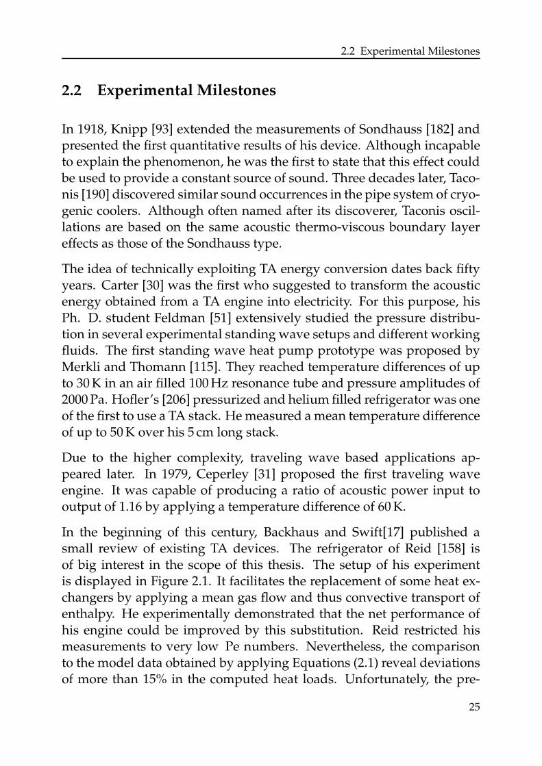
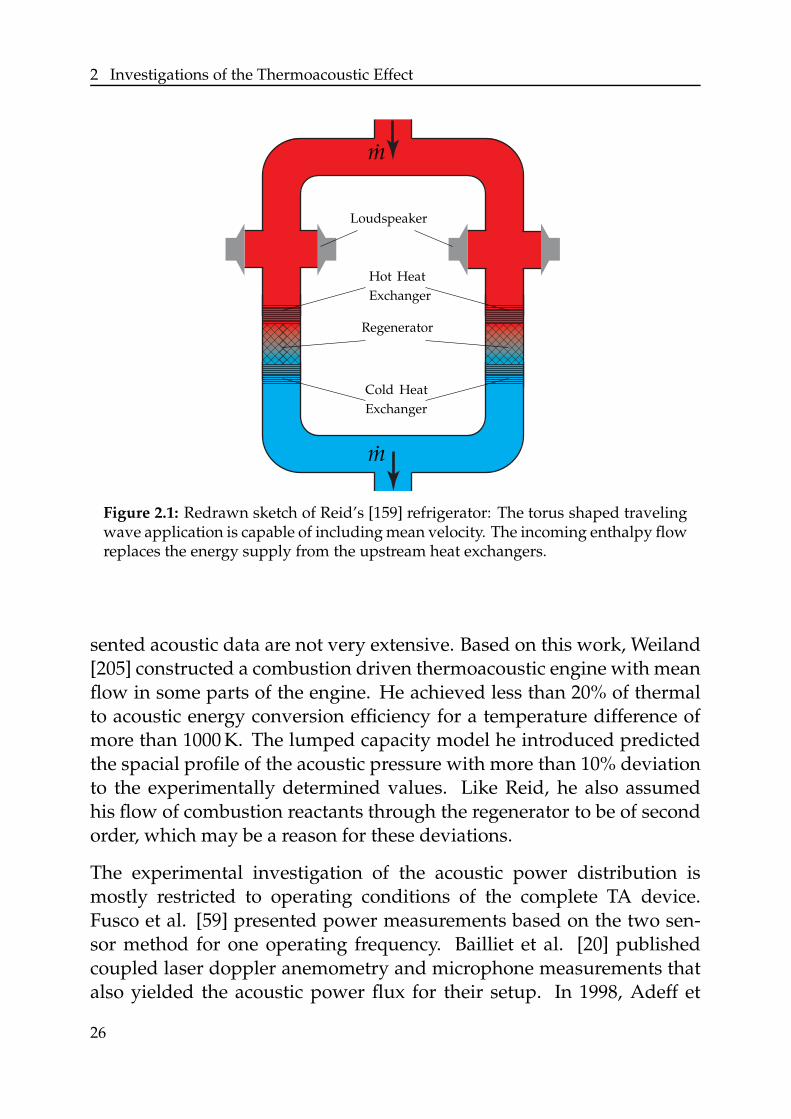
In the beginning of this century, Backhaus and Swift[17] published asmall review of existing TA devices. The refrigerator of Reid [158] isof big interest in the scope of this thesis. The setup of his experimentis displayed in Figure 2.1. It facilitates the replacement of some heat ex-changers by applying a mean gas flow and thus convective transport ofenthalpy. He experimentally demonstrated that the net performance ofhis engine could be improved by this substitution. Reid restricted hismeasurements to very low Pe numbers. Nevertheless, the comparisonto the model data obtained by applying Equations (2.1) reveal deviationsof more than 15% in the computed heat loads. Unfortunately, the pre-
25
2 Investigations of the Thermoacoustic Effect
Cold Heat
Exchanger
Regenerator
Hot Heat
Exchanger
Loudspeaker
m
m
Figure 2.1: Redrawn sketch of Reid’s [159] refrigerator: The torus shaped travelingwave application is capable of including mean velocity. The incoming enthalpy flowreplaces the energy supply from the upstream heat exchangers.
sented acoustic data are not very extensive. Based on this work, Weiland[205] constructed a combustion driven thermoacoustic engine with meanflow in some parts of the engine. He achieved less than 20% of thermalto acoustic energy conversion efficiency for a temperature difference ofmore than 1000 K. The lumped capacity model he introduced predictedthe spacial profile of the acoustic pressure with more than 10% deviationto the experimentally determined values. Like Reid, he also assumedhis flow of combustion reactants through the regenerator to be of secondorder, which may be a reason for these deviations.
The experimental investigation of the acoustic power distribution ismostly restricted to operating conditions of the complete TA device.Fusco et al. [59] presented power measurements based on the two sen-sor method for one operating frequency. Bailliet et al. [20] publishedcoupled laser doppler anemometry and microphone measurements thatalso yielded the acoustic power flux for their setup. In 1998, Adeff et
26
2.3 Numerical Developments
al. [5] investigated stacks made of reticulated vitreous carbon 2 applyingFusco’s technique. One year later Petrulescu et al. [138] experimentallydetermined the working compressibilities of a circular pore with goodagreement to analytically modeled data.
The acoustic scattering caused by TA components is rarely consideredin literature. Only Guedra et al. [66] published very recently acoustictransfer measurement data of a complete thermoacoustic core that is the re-generators flanked by two heat exchangers, a thermal relaxation tube andan additional cold heat exchanger to maintain the outlets at cold condi-tions. They aimed to theoretically derive a criterion leading to instabilityin different applications with the same mounted TA core. The investi-gated frequency ranges from 50 to 200 Hz. In acoustic boundary layertheory the Womersley number
Wo =R
δν, (2.2)
that is the ratio of hydraulic radius R to viscous boundary layer thicknessδν is taken to be the dimensionless number representing the impact offrequency. Substitution into Equation (1.1) leads to a square root scalingof the frequency to this dimensionless number. Thus, Guedra et al. [66]investigate a very small range of 1
6 . Wo . 12 .
2.3 Numerical Developments
The immense increase in computational resources over the last decadescaused a flood of publications treating full and partial numerical simula-tions of TA devices.
The numerical prediction of TA phenomena started in 1994 with theone-dimensional computational tool developed by Swift’s student Ward[203]. This tool works on a coupled system of acoustic network elementsand components describing the regenerators in terms of Rott’s equationsfor one sample pore. Applying a shooting method [154] for some op-timization parameters, the operating conditions of a TA device can be
2 Reticulated Vitreous Carbon or RVC is a foam of glassy carbon, which consists of completely repeatable,regular, and uniform cells. It is a rigid, highly porous and permeable structure.
27
2 Investigations of the Thermoacoustic Effect
predicted. An updated version of the tool3 is used for validation of themodel presented in Chapter 4, which is common for state of the art pub-lications [32]. Although the Reverse Polish Notation and the numeri-cal methods applied are outdated, no other one-dimensional approach iscompetitive to this tool. It is still the choice of most scientists for the firststage of designing TA devices [1].
Up to now, the computational costs for resolving all relevant length scalesthat are geometry, acoustics and boundary layers, are too high for simu-lating a full TA device. Therefore, particular components of the engineare considered, the regenerator and heat exchangers are modeled or thedimensions are reduced. Nijeholt et al. [128] for example performed afull CFD simulation of a traveling wave engine describing the regenera-tor in terms of porous media. Hiereche et al. [70] considered the onset ofa TA engine numerically. Typically, this onset, defined as the initial desta-bilization of a TA device if a critical temperature gradient is exceeded, isoften discussed in experimental investigations [137]. Hiereche and hisco-authors compared the onset of a of a quasi one-dimensional model toa two-dimensional finite volume based simulation of a single stack poreflanked by two idealized heat exchangers. The attached resonator tubeswere described by impedance boundary conditions located at a certaindistance away of the core elements. The same approach was used byBlanc et al. [26, 113] to investigate their TA refrigerator components.Worlikar and Knio [210, 211] described the thermoacoustics inside onepore by a finite difference approach of a linearized dimensionless systemof equations.
The first full 2D-CFD simulation of a very simple TA engine was per-formed in 2007 by Yu et al. [215]. They managed to resolve all scaleswith less than one million cells. The timestep of their simulation was farbeyond the critical acoustic Courant-Friedrichs-Lewis (CFL) number
CFL =c∆t
∆y(2.3)
of unity. Nevertheless, their computational results were quite accurate.The group of Zink investigated the influence of different resonators in atwo dimensionally resolved simple TA engine [219] and demonstrated
3 DeltaEC, Version 6.2, 2008 [202]
28
2.4 Generic Reference Problem
the capability of simulating TA cooling with a commercial CFD code[220]. For the latter, they performed their simulations at a super com-puter. The time step used was orders of magnitudes smaller than thetime step of Yu [215]. It was still too high (CFL&10) to capture all acous-tic effects.
2.4 Generic Reference Problem
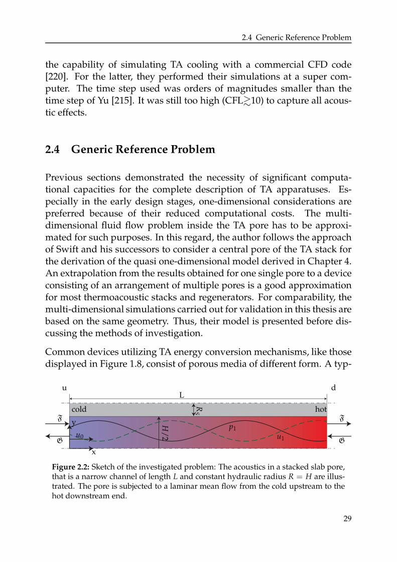
Previous sections demonstrated the necessity of significant computa-tional capacities for the complete description of TA apparatuses. Es-pecially in the early design stages, one-dimensional considerations arepreferred because of their reduced computational costs. The multi-dimensional fluid flow problem inside the TA pore has to be approxi-mated for such purposes. In this regard, the author follows the approachof Swift and his successors to consider a central pore of the TA stack forthe derivation of the quasi one-dimensional model derived in Chapter 4.An extrapolation from the results obtained for one single pore to a deviceconsisting of an arrangement of multiple pores is a good approximationfor most thermoacoustic stacks and regenerators. For comparability, themulti-dimensional simulations carried out for validation in this thesis arebased on the same geometry. Thus, their model is presented before dis-cussing the methods of investigation.
Common devices utilizing TA energy conversion mechanisms, like thosedisplayed in Figure 1.8, consist of porous media of different form. A typ-
50
L
H/
2
RS
FF
GG
y
x
hotcold
du
u0 u1
p1
Figure 2.2: Sketch of the investigated problem: The acoustics in a stacked slab pore,that is a narrow channel of length L and constant hydraulic radius R = H are illus-trated. The pore is subjected to a laminar mean flow from the cold upstream to thehot downstream end.
29
2 Investigations of the Thermoacoustic Effect
ical, rather regular form of porosity is a combination of narrow channels,that is a stack of parallel plates. In this study, one of the channels of sucha TA stack with imposed mean flow and preliminarily determined tem-perature profiles is considered. The geometry of this problem is depictedin Figure 2.2. As the problem is symmetric, only half a pore and thecorresponding half of a solid plate have to be considered. The inlet andoutlet planes of the domain are located at the ends of the solid medium.In this generic configuration, the impact of gravity is ignored as well asentrance or streaming effects. The air flow inside the domain of length Land hydraulic radius R = H is assumed to be laminar [18].
The solid component with a thickness of 2RS is of cordierite with presetconstant material properties. The origin of the Cartesian coordinate sys-tem is located at the cold – or upstream (index u) – end of the channel.The opposite hot end at x = L is also denoted as the downstream (d) endof the pore. The reference values at the cold end of the slab pore are fixedto standard ambient temperature and pressure (SATP [124]).
The propagation of acoustic waves inside the domain under investiga-tion are considered in terms of acoustic pressure p1 and transversallyaveraged velocity 〈u1〉. The incoming and outgoing values are furtherdescribed in terms of characteristic wave amplitudes F,G. For furtherdetails, please refer to Section 3.2.3.
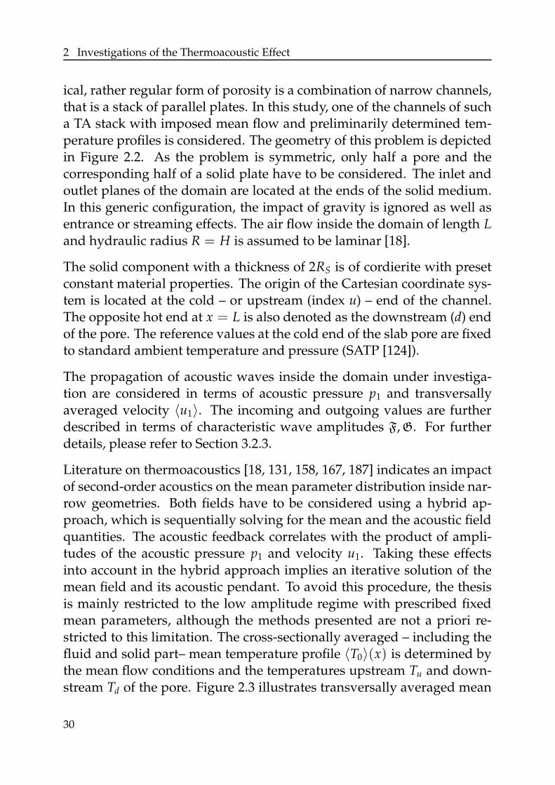
Literature on thermoacoustics [18, 131, 158, 167, 187] indicates an impactof second-order acoustics on the mean parameter distribution inside nar-row geometries. Both fields have to be considered using a hybrid ap-proach, which is sequentially solving for the mean and the acoustic fieldquantities. The acoustic feedback correlates with the product of ampli-tudes of the acoustic pressure p1 and velocity u1. Taking these effectsinto account in the hybrid approach implies an iterative solution of themean field and its acoustic pendant. To avoid this procedure, the thesisis mainly restricted to the low amplitude regime with prescribed fixedmean parameters, although the methods presented are not a priori re-stricted to this limitation. The cross-sectionally averaged – including thefluid and solid part– mean temperature profile 〈T0〉(x) is determined bythe mean flow conditions and the temperatures upstream Tu and down-stream Td of the pore. Figure 2.3 illustrates transversally averaged mean
30
2.4 Generic Reference Problem
00
1
1
0.25
0.25
0.75
0.75
0.5
0.5
Tem
per
atu
re〈T
0〉−
Tu
Td−
Tu[−
]
Position xL [−]
u0 = 0u0 > 0u0 < 0
Figure 2.3: Cross-sectionally averaged mean temperature profiles 〈T0〉(x) (includ-ing the solid temperature) inside a narrow pore. Depending on the mean flowvelocity profile u0(x), the temperature distribution is linear (black) or exponentialshaped.
temperature profiles 〈T0〉(x) for three different flow conditions. If heatconduction inside the solid and fluid media dominates (e.g. u0 = 0), thecross-sectionally averaged temperature gradient ∂〈T0〉/∂x is nearly con-stant. Otherwise, if the Peclet number
Pe =0cpu0L
K(2.4)
is not negligible (u0 6= 0), the temperature profile follows a mixed con-vection/ diffusion transport equation.
Assuming temperature independent thermophysical properties allowsfor an analytical solution of the transversally averaged problem. Giventwo temperature boundary conditions leads to quasi exponential axialtemperature profiles 〈T0(x)〉 (a more detailed consideration is presentedin Section 4.3). Depending on the direction of the flow, the curve is ei-ther convex (blue crosses) for positive velocity or concave (red circles) iffor the counter directed case. The mathematical formulations for thesecorrelations read
∂2T0(x)
∂x2> 0 for u0 > 0 (2.5)
∂2T0(x)
∂x2< 0 for u0 < 0. (2.6)
31

2 Investigations of the Thermoacoustic Effect
The real shape of the curve is always determined from a steady statesolution with non-constant thermophysical properties, leading to smalldeviations from the depicted profiles.
32
3 Theoretical Background
This chapter gives an introduction to the theoretical background of theanalytical models used throughout this thesis. The first section providesdifferent forms of basic equations of fluid dynamics. Starting from themost general formulations of high complexity, they are simplified to ac-count for special conditions. The description of the aeroacoustic trans-port in isentropic conditions is one of these cases. This thesis concen-trates on (thermo-)acoustic problems. The corresponding equations arediscussed in detail in Section 3.2. These formulations form the funda-mentals for acoustic network modeling. An efficiency criterion basedon acoustic two-ports is introduced, whic facilitates a comparison of dif-ferent configurations. The chapter concludes with a review of the GFmethod, which yields a model reduction in Chapter 4.
3.1 Basic Equations of Fluiddynamics
As stated in Section 1.4, this thesis deals with different approaches offluidmechanics and acoustics to describe the physics in TA regeneratorsand its surrounding parts. The most complex approach used here is thefinite volume based CFD technique applied in Chapter 5. The basic equa-tions discretized by this technique as well as the one-dimensional lin-earized transport equations derived in Chapter 4 are based on the sameset of conservation equations describing continuous fluid flow. The re-sulting formalisms arise from different simplifications and discretizationmethods. As the problem considered does not include any chemical re-actions, heat addition or energy production by thermal or nuclear ra-diation, no source terms need to be considered. Many thermoacousticapparatuses experience streaming effects which are initiated by inhomo-geneities caused by gravity. As these effects are beyond the scope of thisthesis, gravity effects are also neglected. Nevertheless, the correspond-ing equations include a general volume force term b. These equationsare part of many textbooks, in which various notations are used. In this
33
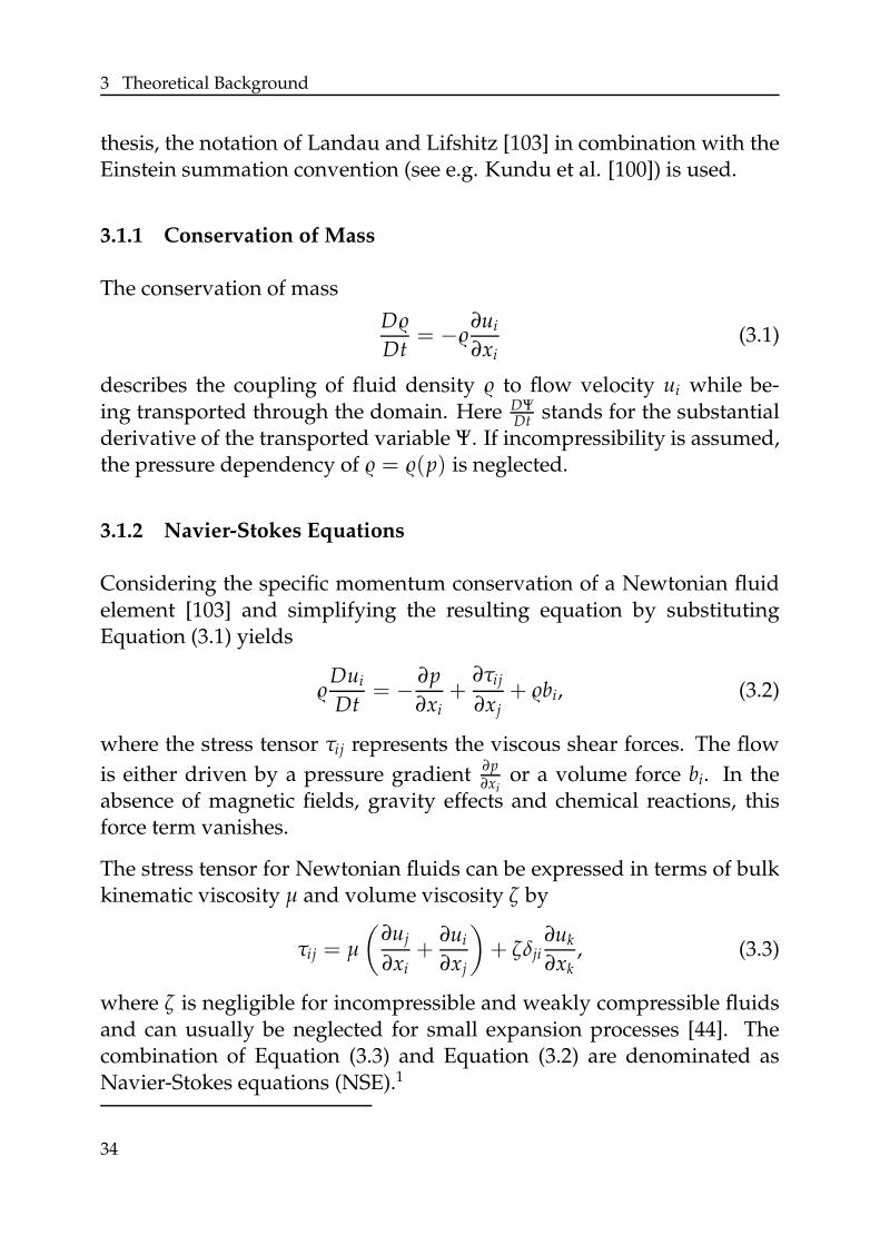
3 Theoretical Background
thesis, the notation of Landau and Lifshitz [103] in combination with theEinstein summation convention (see e.g. Kundu et al. [100]) is used.
3.1.1 Conservation of Mass
The conservation of mass
D
Dt= −
∂ui
∂xi(3.1)
describes the coupling of fluid density to flow velocity ui while be-ing transported through the domain. Here DΨ
Dt stands for the substantialderivative of the transported variable Ψ. If incompressibility is assumed,the pressure dependency of = (p) is neglected.
3.1.2 Navier-Stokes Equations
Considering the specific momentum conservation of a Newtonian fluidelement [103] and simplifying the resulting equation by substitutingEquation (3.1) yields
Dui
Dt= − ∂p
∂xi+
∂τij
∂xj+ bi, (3.2)
where the stress tensor τij represents the viscous shear forces. The flow
is either driven by a pressure gradient ∂p∂xi
or a volume force bi. In theabsence of magnetic fields, gravity effects and chemical reactions, thisforce term vanishes.
The stress tensor for Newtonian fluids can be expressed in terms of bulkkinematic viscosity µ and volume viscosity ζ by
τij = µ
(∂uj
∂xi+
∂ui
∂xj
)
+ ζδji∂uk
∂xk, (3.3)
where ζ is negligible for incompressible and weakly compressible fluidsand can usually be neglected for small expansion processes [44]. Thecombination of Equation (3.3) and Equation (3.2) are denominated asNavier-Stokes equations (NSE).1
34
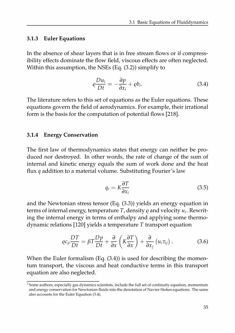
3.1 Basic Equations of Fluiddynamics
3.1.3 Euler Equations
In the absence of shear layers that is in free stream flows or if compress-ibility effects dominate the flow field, viscous effects are often neglected.Within this assumption, the NSEs (Eq. (3.2)) simplify to
Dui
Dt= − ∂p
∂xi+ bi. (3.4)
The literature refers to this set of equations as the Euler equations. Theseequations govern the field of aerodynamics. For example, their irrationalform is the basis for the computation of potential flows [218].
3.1.4 Energy Conservation
The first law of thermodynamics states that energy can neither be pro-duced nor destroyed. In other words, the rate of change of the sum ofinternal and kinetic energy equals the sum of work done and the heatflux q addition to a material volume. Substituting Fourier’s law
qi = K∂T
∂xi(3.5)
and the Newtonian stress tensor (Eq. (3.3)) yields an energy equation interms of internal energy, temperature T, density and velocity ui. Rewrit-ing the internal energy in terms of enthalpy and applying some thermo-dynamic relations [120] yields a temperature T transport equation
cpDT
Dt= βT
Dp
Dt+
∂
∂x
(
K∂T
∂x
)
+∂
∂xj
(uiτij
). (3.6)
When the Euler formalism (Eq. (3.4)) is used for describing the momen-tum transport, the viscous and heat conductive terms in this transportequation are also neglected.
1 Some authors, especially gas dynamics scientists, include the full set of continuity equation, momentumand energy conservation for Newtonian fluids into the denotation of Navier-Stokes equations. The samealso accounts for the Euler Equation (3.4).
35
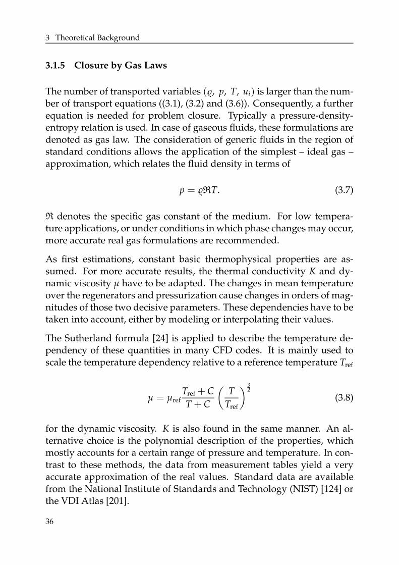
3 Theoretical Background
3.1.5 Closure by Gas Laws
The number of transported variables (, p, T, ui) is larger than the num-ber of transport equations ((3.1), (3.2) and (3.6)). Consequently, a furtherequation is needed for problem closure. Typically a pressure-density-entropy relation is used. In case of gaseous fluids, these formulations aredenoted as gas law. The consideration of generic fluids in the region ofstandard conditions allows the application of the simplest – ideal gas –approximation, which relates the fluid density in terms of
p = RT. (3.7)
R denotes the specific gas constant of the medium. For low tempera-ture applications, or under conditions in which phase changes may occur,more accurate real gas formulations are recommended.
As first estimations, constant basic thermophysical properties are as-sumed. For more accurate results, the thermal conductivity K and dy-namic viscosity µ have to be adapted. The changes in mean temperatureover the regenerators and pressurization cause changes in orders of mag-nitudes of those two decisive parameters. These dependencies have to betaken into account, either by modeling or interpolating their values.
The Sutherland formula [24] is applied to describe the temperature de-pendency of these quantities in many CFD codes. It is mainly used toscale the temperature dependency relative to a reference temperature Tref
µ = µrefTref + C
T + C
(T
Tref
) 32
(3.8)
for the dynamic viscosity. K is also found in the same manner. An al-ternative choice is the polynomial description of the properties, whichmostly accounts for a certain range of pressure and temperature. In con-trast to these methods, the data from measurement tables yield a veryaccurate approximation of the real values. Standard data are availablefrom the National Institute of Standards and Technology (NIST) [124] orthe VDI Atlas [201].
36
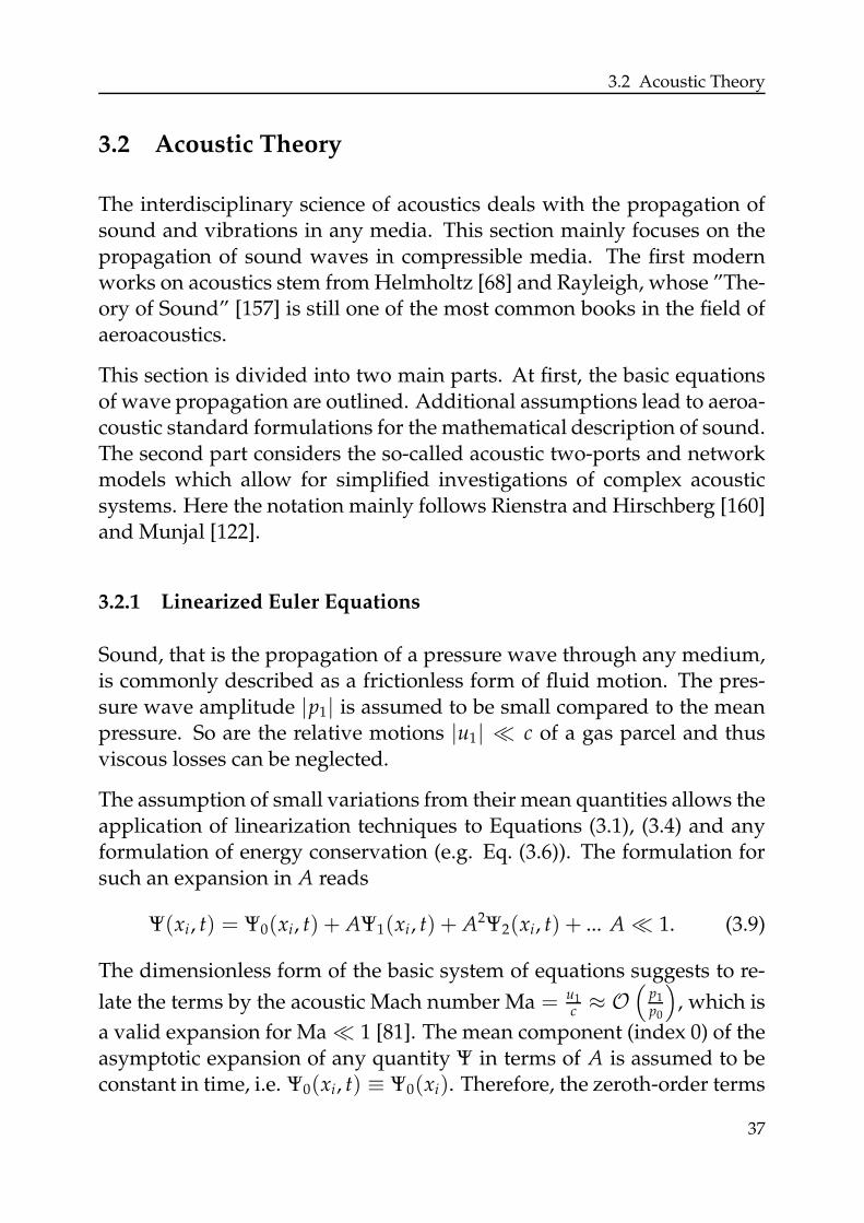
3.2 Acoustic Theory
3.2 Acoustic Theory
The interdisciplinary science of acoustics deals with the propagation ofsound and vibrations in any media. This section mainly focuses on thepropagation of sound waves in compressible media. The first modernworks on acoustics stem from Helmholtz [68] and Rayleigh, whose ”The-ory of Sound” [157] is still one of the most common books in the field ofaeroacoustics.
This section is divided into two main parts. At first, the basic equationsof wave propagation are outlined. Additional assumptions lead to aeroa-coustic standard formulations for the mathematical description of sound.The second part considers the so-called acoustic two-ports and networkmodels which allow for simplified investigations of complex acousticsystems. Here the notation mainly follows Rienstra and Hirschberg [160]and Munjal [122].
3.2.1 Linearized Euler Equations
Sound, that is the propagation of a pressure wave through any medium,is commonly described as a frictionless form of fluid motion. The pres-sure wave amplitude |p1| is assumed to be small compared to the meanpressure. So are the relative motions |u1| ≪ c of a gas parcel and thusviscous losses can be neglected.
The assumption of small variations from their mean quantities allows theapplication of linearization techniques to Equations (3.1), (3.4) and anyformulation of energy conservation (e.g. Eq. (3.6)). The formulation forsuch an expansion in A reads
Ψ(xi, t) = Ψ0(xi, t) + AΨ1(xi, t) + A2Ψ2(xi, t) + ... A ≪ 1. (3.9)
The dimensionless form of the basic system of equations suggests to re-
late the terms by the acoustic Mach number Ma = u1c ≈ O
(p1p0
)
, which is
a valid expansion for Ma ≪ 1 [81]. The mean component (index 0) of theasymptotic expansion of any quantity Ψ in terms of A is assumed to beconstant in time, i.e. Ψ0(xi, t) ≡ Ψ0(xi). Therefore, the zeroth-order terms
37
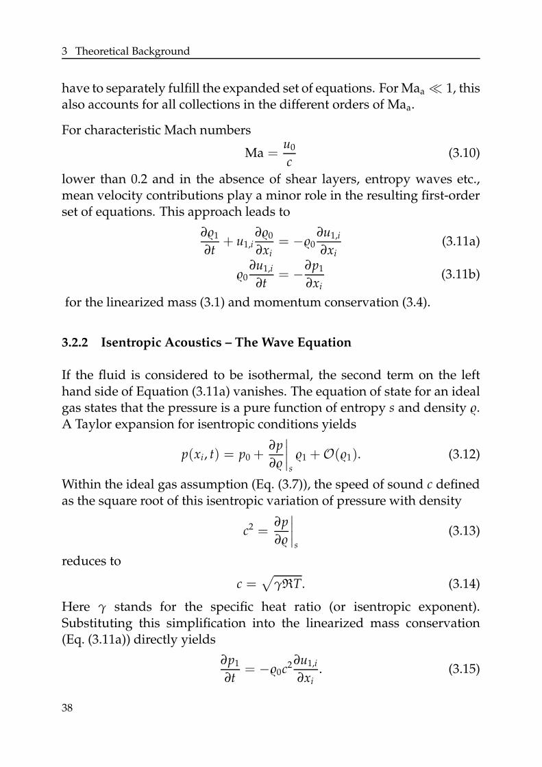
3 Theoretical Background
have to separately fulfill the expanded set of equations. For Maa ≪ 1, thisalso accounts for all collections in the different orders of Maa.
For characteristic Mach numbers
Ma =u0
c(3.10)
lower than 0.2 and in the absence of shear layers, entropy waves etc.,mean velocity contributions play a minor role in the resulting first-orderset of equations. This approach leads to
∂1
∂t+ u1,i
∂0
∂xi= −0
∂u1,i
∂xi(3.11a)
0∂u1,i
∂t= −∂p1
∂xi(3.11b)
for the linearized mass (3.1) and momentum conservation (3.4).
3.2.2 Isentropic Acoustics – The Wave Equation
If the fluid is considered to be isothermal, the second term on the lefthand side of Equation (3.11a) vanishes. The equation of state for an idealgas states that the pressure is a pure function of entropy s and density .A Taylor expansion for isentropic conditions yields
p(xi, t) = p0 +∂p
∂
∣∣∣∣
s
1 +O(1). (3.12)
Within the ideal gas assumption (Eq. (3.7)), the speed of sound c definedas the square root of this isentropic variation of pressure with density
c2 =∂p
∂
∣∣∣∣
s
(3.13)
reduces to
c =√
γRT. (3.14)
Here γ stands for the specific heat ratio (or isentropic exponent).Substituting this simplification into the linearized mass conservation(Eq. (3.11a)) directly yields
∂p1
∂t= −0c2 ∂u1,i
∂xi. (3.15)
38
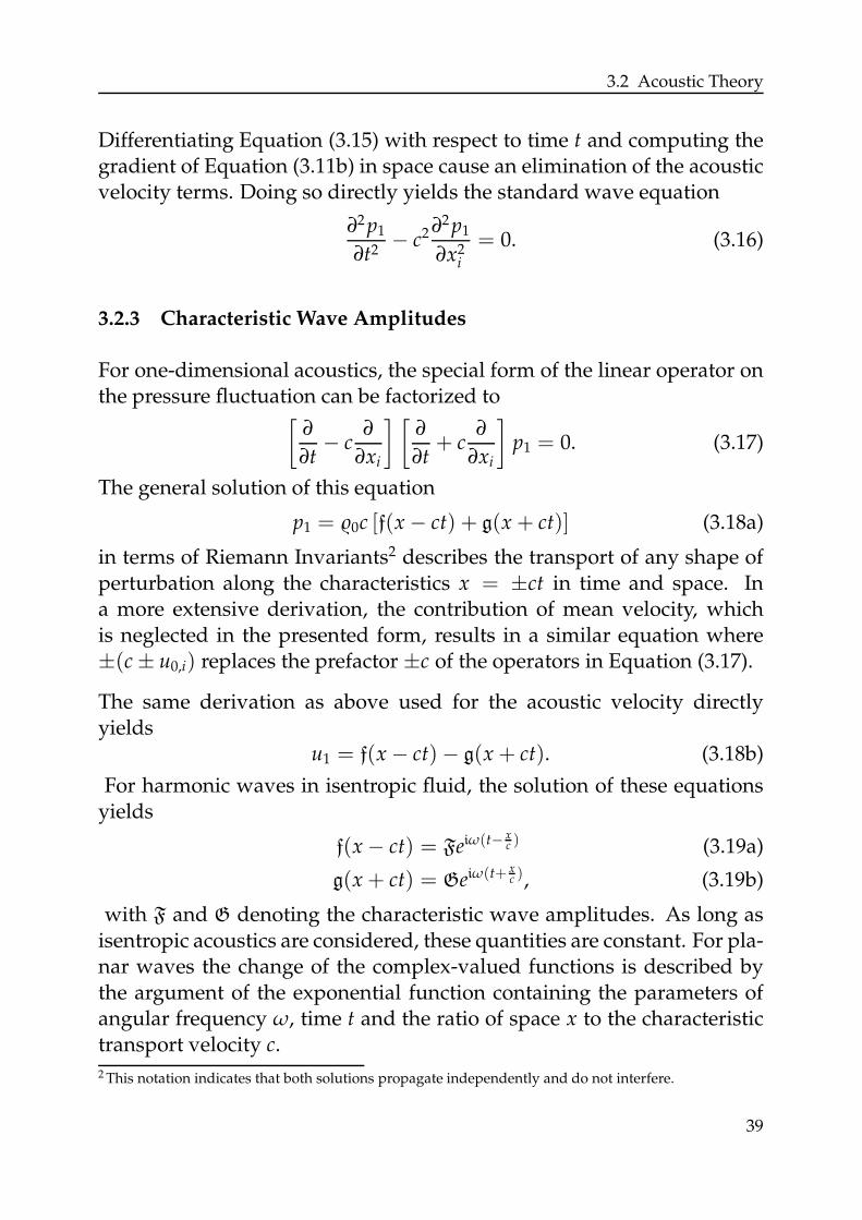
3.2 Acoustic Theory
Differentiating Equation (3.15) with respect to time t and computing thegradient of Equation (3.11b) in space cause an elimination of the acousticvelocity terms. Doing so directly yields the standard wave equation
∂2 p1
∂t2− c2 ∂2 p1
∂x2i
= 0. (3.16)
3.2.3 Characteristic Wave Amplitudes
For one-dimensional acoustics, the special form of the linear operator onthe pressure fluctuation can be factorized to
[∂
∂t− c
∂
∂xi
] [∂
∂t+ c
∂
∂xi
]
p1 = 0. (3.17)
The general solution of this equation
p1 = 0c [f(x − ct) + g(x + ct)] (3.18a)
in terms of Riemann Invariants2 describes the transport of any shape ofperturbation along the characteristics x = ±ct in time and space. Ina more extensive derivation, the contribution of mean velocity, whichis neglected in the presented form, results in a similar equation where±(c ± u0,i) replaces the prefactor ±c of the operators in Equation (3.17).
The same derivation as above used for the acoustic velocity directlyyields
u1 = f(x − ct)− g(x + ct). (3.18b)
For harmonic waves in isentropic fluid, the solution of these equationsyields
f(x − ct) = Feiω(t− xc ) (3.19a)
g(x + ct) = Geiω(t+ xc ), (3.19b)
with F and G denoting the characteristic wave amplitudes. As long asisentropic acoustics are considered, these quantities are constant. For pla-nar waves the change of the complex-valued functions is described bythe argument of the exponential function containing the parameters ofangular frequency ω, time t and the ratio of space x to the characteristictransport velocity c.
2 This notation indicates that both solutions propagate independently and do not interfere.
39
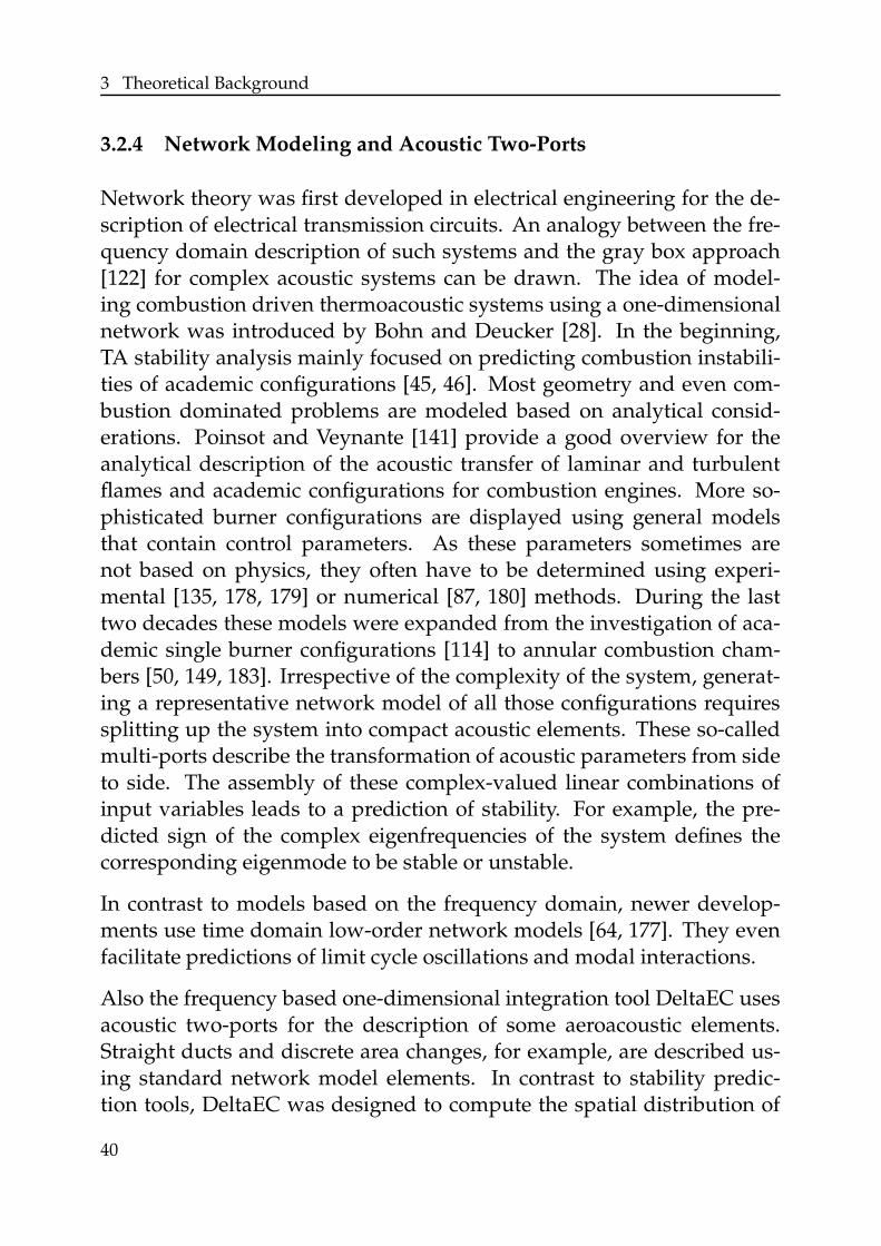
3 Theoretical Background
3.2.4 Network Modeling and Acoustic Two-Ports
Network theory was first developed in electrical engineering for the de-scription of electrical transmission circuits. An analogy between the fre-quency domain description of such systems and the gray box approach[122] for complex acoustic systems can be drawn. The idea of model-ing combustion driven thermoacoustic systems using a one-dimensionalnetwork was introduced by Bohn and Deucker [28]. In the beginning,TA stability analysis mainly focused on predicting combustion instabili-ties of academic configurations [45, 46]. Most geometry and even com-bustion dominated problems are modeled based on analytical consid-erations. Poinsot and Veynante [141] provide a good overview for theanalytical description of the acoustic transfer of laminar and turbulentflames and academic configurations for combustion engines. More so-phisticated burner configurations are displayed using general modelsthat contain control parameters. As these parameters sometimes arenot based on physics, they often have to be determined using experi-mental [135, 178, 179] or numerical [87, 180] methods. During the lasttwo decades these models were expanded from the investigation of aca-demic single burner configurations [114] to annular combustion cham-bers [50, 149, 183]. Irrespective of the complexity of the system, generat-ing a representative network model of all those configurations requiressplitting up the system into compact acoustic elements. These so-calledmulti-ports describe the transformation of acoustic parameters from sideto side. The assembly of these complex-valued linear combinations ofinput variables leads to a prediction of stability. For example, the pre-dicted sign of the complex eigenfrequencies of the system defines thecorresponding eigenmode to be stable or unstable.
In contrast to models based on the frequency domain, newer develop-ments use time domain low-order network models [64, 177]. They evenfacilitate predictions of limit cycle oscillations and modal interactions.
Also the frequency based one-dimensional integration tool DeltaEC usesacoustic two-ports for the description of some aeroacoustic elements.Straight ducts and discrete area changes, for example, are described us-ing standard network model elements. In contrast to stability predic-tion tools, DeltaEC was designed to compute the spatial distribution of
40
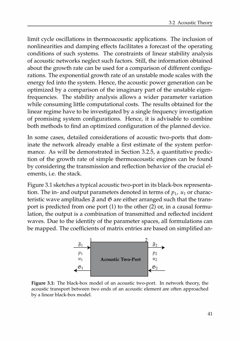
3.2 Acoustic Theory
limit cycle oscillations in thermoacoustic applications. The inclusion ofnonlinearities and damping effects facilitates a forecast of the operatingconditions of such systems. The constraints of linear stability analysisof acoustic networks neglect such factors. Still, the information obtainedabout the growth rate can be used for a comparison of different configu-rations. The exponential growth rate of an unstable mode scales with theenergy fed into the system. Hence, the acoustic power generation can beoptimized by a comparison of the imaginary part of the unstable eigen-frequencies. The stability analysis allows a wider parameter variationwhile consuming little computational costs. The results obtained for thelinear regime have to be investigated by a single frequency investigationof promising system configurations. Hence, it is advisable to combineboth methods to find an optimized configuration of the planned device.
In some cases, detailed considerations of acoustic two-ports that dom-inate the network already enable a first estimate of the system perfor-mance. As will be demonstrated in Section 3.2.5, a quantitative predic-tion of the growth rate of simple thermoacoustic engines can be foundby considering the transmission and reflection behavior of the crucial el-ements, i.e. the stack.
Figure 3.1 sketches a typical acoustic two-port in its black-box representa-tion. The in- and output parameters denoted in terms of p1, u1 or charac-teristic wave amplitudes F and G are either arranged such that the trans-port is predicted from one port (1) to the other (2) or, in a causal formu-lation, the output is a combination of transmitted and reflected incidentwaves. Due to the identity of the parameter spaces, all formulations canbe mapped. The coefficients of matrix entries are based on simplified an-
21F1
G1
F2
G2
p1
u1
p2
u2Acoustic Two-Port
Figure 3.1: The black-box model of an acoustic two-port. In network theory, theacoustic transport between two ends of an acoustic element are often approachedby a linear black-box model.
41
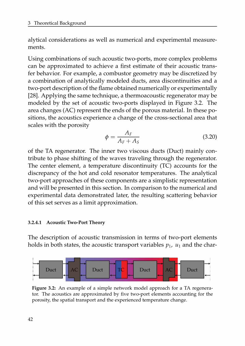
3 Theoretical Background
alytical considerations as well as numerical and experimental measure-ments.
Using combinations of such acoustic two-ports, more complex problemscan be approximated to achieve a first estimate of their acoustic trans-fer behavior. For example, a combustor geometry may be discretized bya combination of analytically modeled ducts, area discontinuities and atwo-port description of the flame obtained numerically or experimentally[28]. Applying the same technique, a thermoacoustic regenerator may bemodeled by the set of acoustic two-ports displayed in Figure 3.2. Thearea changes (AC) represent the ends of the porous material. In these po-sitions, the acoustics experience a change of the cross-sectional area thatscales with the porosity
φ =AF
AF + AS(3.20)
of the TA regenerator. The inner two viscous ducts (Duct) mainly con-tribute to phase shifting of the waves traveling through the regenerator.The center element, a temperature discontinuity (TC) accounts for thediscrepancy of the hot and cold resonator temperatures. The analyticaltwo-port approaches of these components are a simplistic representationand will be presented in this section. In comparison to the numerical andexperimental data demonstrated later, the resulting scattering behaviorof this set serves as a limit approximation.
3.2.4.1 Acoustic Two-Port Theory
The description of acoustic transmission in terms of two-port elementsholds in both states, the acoustic transport variables p1, u1 and the char-
300
Duct AC Duct TC Duct AC Duct
Figure 3.2: An example of a simple network model approach for a TA regenera-tor. The acoustics are approximated by five two-port elements accounting for theporosity, the spatial transport and the experienced temperature change.
42
3.2 Acoustic Theory
acteristic wave space F, G. This section provides the relations betweenthe different notations.
Transfer Matrices
The port to port transmission formulation through a black box elementis generally referred to as transfer matrix T. Scaling the acoustic pressurep1with the specific acoustic impedance 0c leads to non-dimensional ma-trix entries in
(p1
0c
u1
)
2
=
[
T11 T12
T21 T22
](p10c
u1
)
1
= Tpu
(p10c
u1
)
1
. (3.21)
In general, the complex-valued coefficients in Tpu are functions of fre-quency f and problem-dependent parameters. This formulation is oftenused, because of its plausibility. It allows a direct identification of charac-teristic parameters in analytical models for some network elements. Thetransfer matrix of a flame in a burner for example is often approximatedusing Rankine-Hugoniot relations [141]. Some terms of these equationsscale with characteristic mean temperature ratios or the Mach number ofthe mean flow.
The formulation of Equation (3.21) in the characteristic wave amplitudespace
(
F
G
)
2
=
[
T11 T12
T21 T22
](
F
G
)
1
= TFG
(
F
G
)
1
(3.22)
is mostly used to display short analytical formulations, for example forducts and channels. Introducing the conversion matrix
Ω =1
2
[
1 1
1 −1
]
, (3.23)
it directly couples with the transfer matrix in pu notation by
TFG = ΩTpuΩ−1. (3.24)
One advantage of these notations is their simple mathematical coupling.The matrix product of the series of acoustic elements is equivalent tothe transport through the technical components represented by these el-ements.
43
3 Theoretical Background
Scattering Matrices
If the observer’s interests focuses on the impact of the incoming waves onthe output of the acoustic element, a scattering matrix notation directlyyields this causality. While the diagonal elements t12, t21 in
(
F2
G1
)
=
[
t12 r11
r22 t21
](
F1
G2
)
= S
(
F1
G2
)
(3.25)
describe the transmission of waves, the off-diagonal elements rii displaythe contribution of the reflections to the outgoing wave.
Except for the case of vanishing wave transmission in negative coordi-nate direction, S is directly related to the characteristic wave space trans-fer matrix TFG. Rearranging the matrix components in terms of
S =1
T22
[
T11T22 − T12T21 T12
−T21 1
]
, (3.26)
yields a scattering matrix formulation.
3.2.4.2 Analytical Two-Port Models
The last section provided the basic correlations for acoustic networkmodeling. This section discusses the three analytical approaches, whichare applied in the remainder of this thesis.
Thermo-Viscous Ducts
Formulating the one-dimensional characteristic wave propagation underisentropic conditions (Eqs. (3.19)) in terms of scattering matrices, the in-dependence of solutions F and G directly yields
(
F
G
)
2
=
[
exp (−ik+x) 0
0 exp (ik−x)
](
F
G
)
1
. (3.27)
Here the wave numbers k± are defined by ωc±u . The sign notation is cho-
sen, such that waves traveling in positive flow direction from x1 to x2 are
44
3.2 Acoustic Theory
denoted by +. In duct acoustics, losses in pipes are generally not negligi-ble. The damping influence is mostly taken into account by manipulatingthe wave number with an additional complex-valued term d that scalesthe k± in terms of
k± = dω
c ± u. (3.28)
As damping strongly depends on the geometric conditions, a wide vari-ety of approaches can be found in literature [122, 197]. Preliminary exper-imental investigations by Alemela [7] and Neunert [127] at the Lehrstuhlfur Thermodynamik at TU Munchen revealed good results with the ap-plication of Kirchhoff’s [92] formulation. Using Neunert’s [127] formula-tion and an expected roughness coefficient of unity, the damping coeffi-cient
d = 1 +(1 − i)√
2 Sh
(
1 +γ − 1√
Pr
)
(3.29)
is a function of the Womersley number, Wo, the Prandtl number, Pr andthe Shear number, Sh combining the material properties of the fluid. Thenature of this damping model causes a generation of complex-valued k±,which lead to an exponential decrease of the characteristic wave ampli-tudes while traveling through the duct.
Non-Constant Cross-Sectional Areas
Technical applications of duct acoustics exhibit non-constant cross-sectional areas. Provided that the assumption of acoustic compactnessholds, i.e. as long as the acoustic wave length
λ =c
f(3.30)
is much larger than the geometric length scale, the change in cross-sectional area is considered as an abrupt change in A. If this assumptionis too restrictive, for example for continuously varying cross-sections, adistributed area change can be approximated by a discretized series ofducts and area changes [143].
Such area changes often generate acoustic losses by mean flow interac-tion, for example in the shear layers occurring in the region mean flowexpansion. Such losses are hard to handle qualitatively. Most of them
45
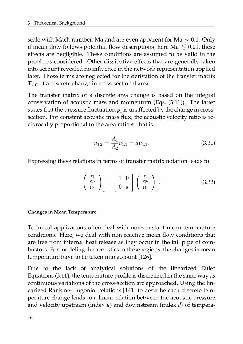
3 Theoretical Background
scale with Mach number, Ma and are even apparent for Ma ∼ 0.1. Onlyif mean flow follows potential flow descriptions, here Ma . 0.01, theseeffects are negligible. These conditions are assumed to be valid in theproblems considered. Other dissipative effects that are generally takeninto account revealed no influence in the network representation appliedlater. These terms are neglected for the derivation of the transfer matrixTAC of a discrete change in cross-sectional area.
The transfer matrix of a discrete area change is based on the integralconservation of acoustic mass and momentum (Eqs. (3.11)). The latterstates that the pressure fluctuation p1 is unaffected by the change in cross-section. For constant acoustic mass flux, the acoustic velocity ratio is re-ciprocally proportional to the area ratio α, that is
u1,2 =A1
A2u1,1 = αu1,1. (3.31)
Expressing these relations in terms of transfer matrix notation leads to
(p1
0c
u1
)
2
=
[
1 0
0 α
](p1
0c
u1
)
1
. (3.32)
Changes in Mean Temperature
Technical applications often deal with non-constant mean temperatureconditions. Here, we deal with non-reactive mean flow conditions thatare free from internal heat release as they occur in the tail pipe of com-bustors. For modeling the acoustics in these regions, the changes in meantemperature have to be taken into account [126].
Due to the lack of analytical solutions of the linearized EulerEquations (3.11), the temperature profile is discretized in the same way ascontinuous variations of the cross-section are approached. Using the lin-earized Rankine-Hugoniot relations [141] to describe each discrete tem-perature change leads to a linear relation between the acoustic pressureand velocity upstream (index u) and downstream (index d) of tempera-
46
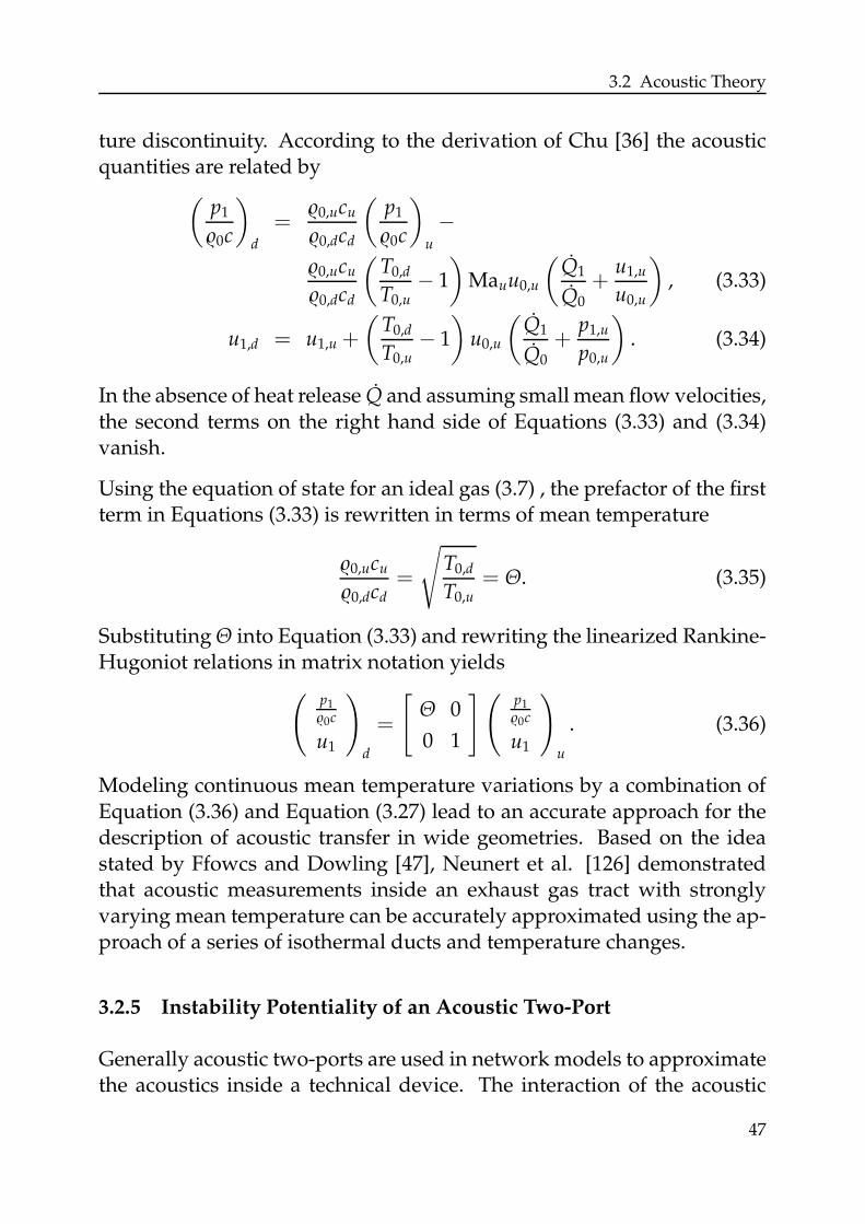
3.2 Acoustic Theory
ture discontinuity. According to the derivation of Chu [36] the acousticquantities are related by
(p1
0c
)
d
=0,ucu
0,dcd
(p1
0c
)
u
−
0,ucu
0,dcd
(T0,d
T0,u− 1
)
Mauu0,u
(Q1
Q0
+u1,u
u0,u
)
, (3.33)
u1,d = u1,u +
(T0,d
T0,u− 1
)
u0,u
(Q1
Q0
+p1,u
p0,u
)
. (3.34)
In the absence of heat release Q and assuming small mean flow velocities,the second terms on the right hand side of Equations (3.33) and (3.34)vanish.
Using the equation of state for an ideal gas (3.7) , the prefactor of the firstterm in Equations (3.33) is rewritten in terms of mean temperature
0,ucu
0,dcd=
√
T0,d
T0,u= Θ. (3.35)
Substituting Θ into Equation (3.33) and rewriting the linearized Rankine-Hugoniot relations in matrix notation yields
(p1
0c
u1
)
d
=
[
Θ 0
0 1
](p1
0c
u1
)
u
. (3.36)
Modeling continuous mean temperature variations by a combination ofEquation (3.36) and Equation (3.27) lead to an accurate approach for thedescription of acoustic transfer in wide geometries. Based on the ideastated by Ffowcs and Dowling [47], Neunert et al. [126] demonstratedthat acoustic measurements inside an exhaust gas tract with stronglyvarying mean temperature can be accurately approximated using the ap-proach of a series of isothermal ducts and temperature changes.
3.2.5 Instability Potentiality of an Acoustic Two-Port
Generally acoustic two-ports are used in network models to approximatethe acoustics inside a technical device. The interaction of the acoustic
47
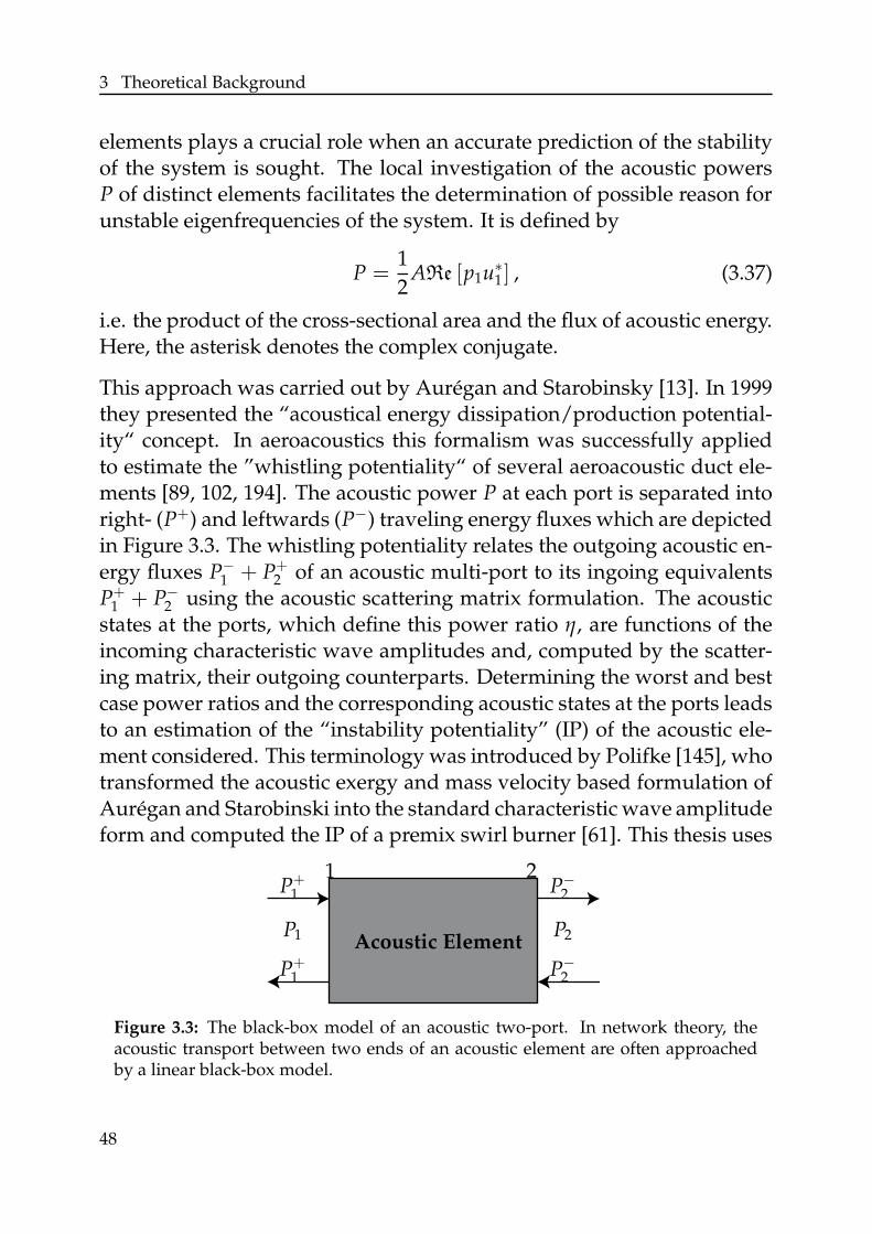
3 Theoretical Background
elements plays a crucial role when an accurate prediction of the stabilityof the system is sought. The local investigation of the acoustic powersP of distinct elements facilitates the determination of possible reason forunstable eigenfrequencies of the system. It is defined by
P =1
2ARe [p1u∗
1 ] , (3.37)
i.e. the product of the cross-sectional area and the flux of acoustic energy.Here, the asterisk denotes the complex conjugate.
This approach was carried out by Auregan and Starobinsky [13]. In 1999they presented the “acoustical energy dissipation/production potential-ity“ concept. In aeroacoustics this formalism was successfully appliedto estimate the ”whistling potentiality“ of several aeroacoustic duct ele-ments [89, 102, 194]. The acoustic power P at each port is separated intoright- (P+) and leftwards (P−) traveling energy fluxes which are depictedin Figure 3.3. The whistling potentiality relates the outgoing acoustic en-ergy fluxes P−
1 + P+2 of an acoustic multi-port to its ingoing equivalents
P+1 + P−
2 using the acoustic scattering matrix formulation. The acousticstates at the ports, which define this power ratio η, are functions of theincoming characteristic wave amplitudes and, computed by the scatter-ing matrix, their outgoing counterparts. Determining the worst and bestcase power ratios and the corresponding acoustic states at the ports leadsto an estimation of the “instability potentiality” (IP) of the acoustic ele-ment considered. This terminology was introduced by Polifke [145], whotransformed the acoustic exergy and mass velocity based formulation ofAuregan and Starobinski into the standard characteristic wave amplitudeform and computed the IP of a premix swirl burner [61]. This thesis uses
21P+
1
P+1
P−2
P−2
P1 P2Acoustic Element
Figure 3.3: The black-box model of an acoustic two-port. In network theory, theacoustic transport between two ends of an acoustic element are often approachedby a linear black-box model.
48
3.2 Acoustic Theory
the formalism to demonstrate the influence of certain parameters on thelimit power ratios of TA stacks. The corresponding acoustic states arenot considered. A deeper investigation of the relevance of these quan-tities for TA applications can be found in Holzinger et al. [73]. As thecharacteristic wave formalism is used in this thesis, the main derivationsteps of IP are briefly repeated in this section maintaining the notation ofPolifke [145].
Using the characteristic waves, the acoustic sound power at the port ofan acoustic element defined by Equation (3.37) reads
P =1
20cA (FF∗ −GG∗) . (3.38)
Defining the variable
χ =
√
cA
2, (3.39)
and inserting
P+ = χF, P− = χG, (3.40)
enables an interpretation of the terms in brackets in Equation (3.38) as thesum of incoming and outgoing acoustic fluxes at this port. Summing upthe sound powers of all ports yields the net production Π of an acousticmulti-port. Defining the input and output vector of a two-port system as
r =
(
P+1
P−2
)
, z =
(
P−1
P+2
)
, (3.41)
this quantity Π readsΠ = r
r − z
z. (3.42)
Next, the order of output wave amplitudes of the scattering matrix nota-tion is changed, such that
S =
[
r11 t12
t21 r22
]
. (3.43)
A multiplication of S by
V =
[
χ1 0
0 χ2
]
(3.44)
49
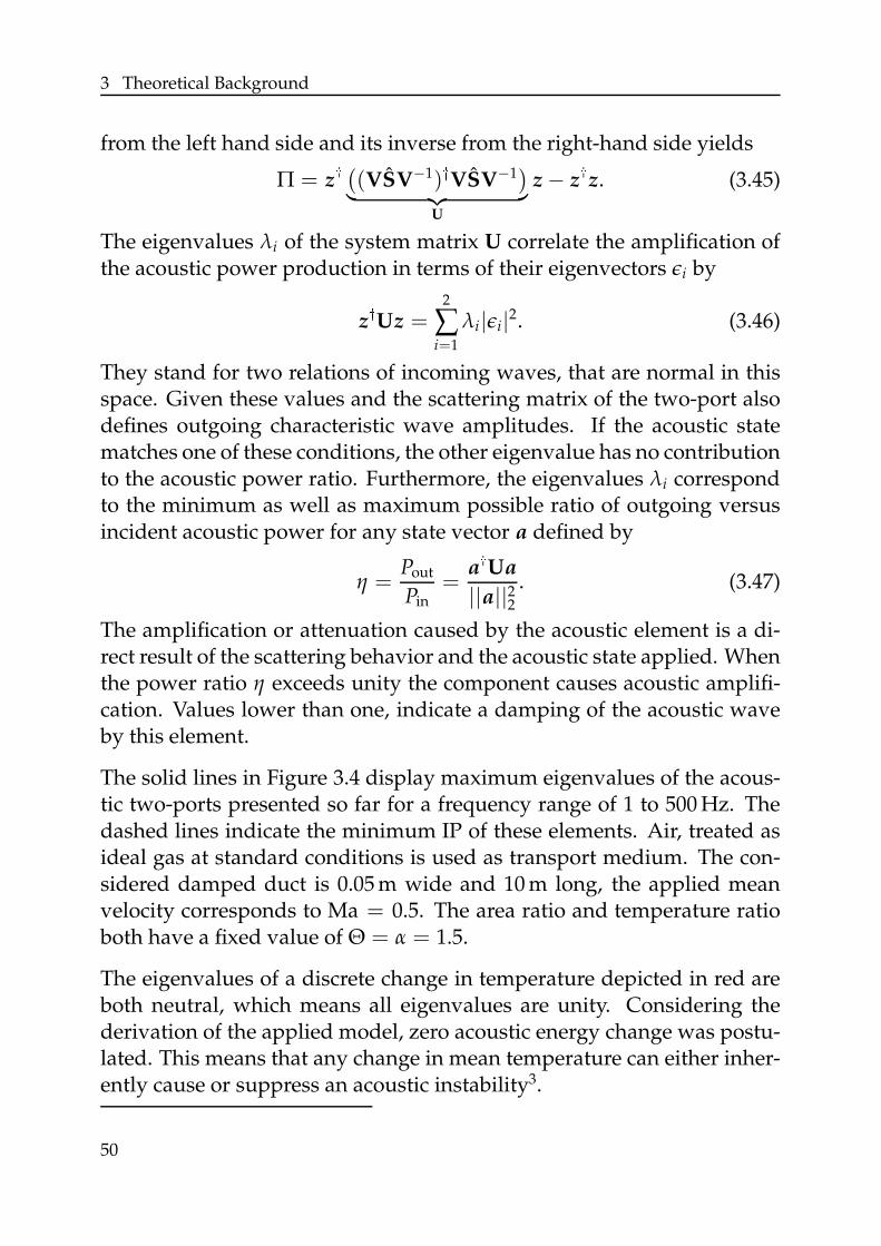
3 Theoretical Background
from the left hand side and its inverse from the right-hand side yields
Π = z
((VSV−1)VSV−1
)
︸ ︷︷ ︸
U
z − z
z. (3.45)
The eigenvalues λi of the system matrix U correlate the amplification ofthe acoustic power production in terms of their eigenvectors ǫi by
zUz =
2
∑i=1
λi|ǫi|2. (3.46)
They stand for two relations of incoming waves, that are normal in thisspace. Given these values and the scattering matrix of the two-port alsodefines outgoing characteristic wave amplitudes. If the acoustic statematches one of these conditions, the other eigenvalue has no contributionto the acoustic power ratio. Furthermore, the eigenvalues λi correspondto the minimum as well as maximum possible ratio of outgoing versusincident acoustic power for any state vector a defined by
η =Pout
Pin=
aUa
||a||22. (3.47)
The amplification or attenuation caused by the acoustic element is a di-rect result of the scattering behavior and the acoustic state applied. Whenthe power ratio η exceeds unity the component causes acoustic amplifi-cation. Values lower than one, indicate a damping of the acoustic waveby this element.
The solid lines in Figure 3.4 display maximum eigenvalues of the acous-tic two-ports presented so far for a frequency range of 1 to 500 Hz. Thedashed lines indicate the minimum IP of these elements. Air, treated asideal gas at standard conditions is used as transport medium. The con-sidered damped duct is 0.05 m wide and 10 m long, the applied meanvelocity corresponds to Ma = 0.5. The area ratio and temperature ratioboth have a fixed value of Θ = α = 1.5.
The eigenvalues of a discrete change in temperature depicted in red areboth neutral, which means all eigenvalues are unity. Considering thederivation of the applied model, zero acoustic energy change was postu-lated. This means that any change in mean temperature can either inher-ently cause or suppress an acoustic instability3.
50
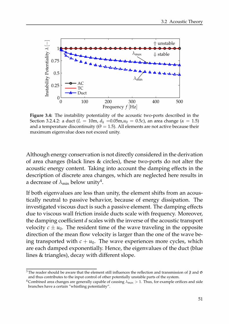
3.2 Acoustic Theory
00
1
0.25
0.75
100 200 300 400 500
0.5
Frequency f [Hz]
Inst
abil
ity
Po
ten
tial
ity
λ[−
]
ACTCDuct
λmax
λmin
⇑ unstable
⇓ stable
Figure 3.4: The instability potentiality of the acoustic two-ports described in theSection 3.2.4.2: a duct (L = 10m, dh =0.05m,u0 = 0.5c), an area change (α = 1.5)and a temperature discontinuity (Θ = 1.5). All elements are not active because theirmaximum eigenvalue does not exceed unity.
Although energy conservation is not directly considered in the derivationof area changes (black lines & circles), these two-ports do not alter theacoustic energy content. Taking into account the damping effects in thedescription of discrete area changes, which are neglected here results ina decrease of λmin below unity4.
If both eigenvalues are less than unity, the element shifts from an acous-tically neutral to passive behavior, because of energy dissipation. Theinvestigated viscous duct is such a passive element. The damping effectsdue to viscous wall friction inside ducts scale with frequency. Moreover,the damping coefficient d scales with the inverse of the acoustic transportvelocity c ± u0. The resident time of the wave traveling in the oppositedirection of the mean flow velocity is larger than the one of the wave be-ing transported with c + u0. The wave experiences more cycles, whichare each damped exponentially. Hence, the eigenvalues of the duct (bluelines & triangles), decay with different slope.
3 The reader should be aware that the element still influences the reflection and transmission of F and G
and thus contributes to the input control of other potentially unstable parts of the system.4 Combined area changes are generally capable of causing λmax > 1. Thus, for example orifices and side
branches have a certain ”whistling potentiality”.
51
3 Theoretical Background
The resonators and most of the thermoacoustic core components allow anetwork description in terms of the three two-ports considered. In classicthermoacoustic engines the stack or regenerator (and for certain configu-rations the heat exchangers) is the only expected acoustic amplifier. Theinstability potentiality of these acoustic elements is a qualitative indica-tion for the amount of acoustic power generated by the complete device.
3.2.6 Analytical Solutions Obtained by the Green’s Function Method
Special conditions allow for a partial simplification of the acoustic equa-tions (NSE and EE) by substituting analytical solutions. In general, theseformulations are derived from solving inhomogeneous linear differentialequations. One of the most powerful tools to produce such solutions isthe application of the Green’s function (GF) method. Its advantage com-pared to most other techniques is that once the solution for the differen-tial operator is obtained, the influence of any right-hand side term canbe obtained by a convolution process. Besides finding analytical solu-tions for acoustic problems, it is applied in various other scientific fields:potential theory [90] and heat conduction [38] problems are investigatedas well as differential equations describing quantum physics [49]. Here,this method is used to reduce the linearized NSEs derived in Chapter 4from a multi-dimensional problem into a set of quasi one-dimensionalordinary differential equations describing the acoustic transport througha TA regenerator.
The characteristic GF G(y|y) of a problem describes the response of thesystem to a Dirac impulse δ(y − y), i.e. a unit impulse located at y. Dueto the nature of this special right-hand side inhomogeneity, the convo-lution of G(y|y) with any other kind of inhomogeneity b(y) yields thecorresponding response of the field.
In mathematical terms, the GF is the solution of the linear differentialoperator L(y) acting on a certain domain y ∈ [ymin, ymax] following
L(y)G(y|y) = δ(y − y). (3.48)
52
3.2 Acoustic Theory
If the same operator L(y) is acting on ϑ(y) in combination with any ar-bitrary inhomogeneity b(y), the solution of ϑ(y) can be easily found by
ϑ(y) =
ymax∫
ymin
G(y|y)b(y) dy. (3.49)
There are different ways for obtaining the GF for a certain L. Variousmethods are provided in textbooks [38, 41, 48], but their presentation isbeyond the scope of this thesis. As the derivation process does not alwayslead to analytical formulations and sometimes is very cumbersome, theGFs determined are also listed in the references provided.
In Chapter 4, this thesis treats problems with a differential operator of theform
L [ϑ(y)] =
[
1 − 1
α2
∂2
∂y2
]
ϑ(y). (3.50)
Here, the complex-valued parameter α is constant in y. With this assump-tion, the corresponding GF reads
G(y|y) = −α H(y − y) sinh(α(y − y)) + C1(y)eαy + C2(y)e
−αy. (3.51)
Here, H(y− y) denotes the Heaviside function. The integration constantsCi are determined by the required boundary conditions (BC). IncludingBCs of first kind (Dirichlet)
ϑ(yj) = gj (3.52)
and second kind (Neumann)
∂ϑ
∂y
∣∣∣∣
yk
= hk, (3.53)
the solution for ϑ(y) reduces to [38]
ϑ(y) =
y=L∫
y=0
G(y|y)b(y) dy +1
α2 ∑j
gjG(y|yj)−1
α2 ∑k
hk∂G(y|y)
∂y
∣∣∣∣
y=yk
.
(3.54)The first term describes the impact of the inhomogeneity. The contri-butions of all BC types scale with α−2. In the investigated problem, the
53

3 Theoretical Background
field is fixed by a Dirichlet condition at the solid/fluid interface. Thecenter of the pore displayed in Figure 2.2 is represented by a symmetryplane. With this BC at yk = 0, hk becomes zero and the third term inEquation (3.54), accounting for Neumann conditions, vanishes.
54
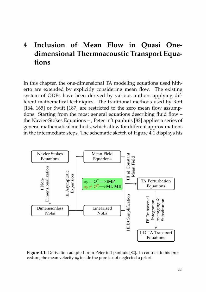
4 Inclusion of Mean Flow in Quasi One-dimensional Thermoacoustic Transport Equa-tions
In this chapter, the one-dimensional TA modeling equations used hith-erto are extended by explicitly considering mean flow. The existingsystem of ODEs have been derived by various authors applying dif-ferent mathematical techniques. The traditional methods used by Rott[164, 165] or Swift [187] are restricted to the zero mean flow assump-tions. Starting from the most general equations describing fluid flow –the Navier-Stokes Equations – , Peter in’t panhuis [82] applies a series ofgeneral mathematical methods, which allow for different approximationsin the intermediate steps. The schematic sketch of Figure 4.1 displays his
Navier-StokesEquations
Mean FieldEquations
u0 = O2=⇒IMPu0 6= O2=⇒MI, MII
LinearizedNSEs
DimensionlessNSEs
TA PerturbationEquations
1-D TA TransportEquations
IN
on
-D
imen
sio
nal
izat
ion
IIA
sym
pto
tic
Ex
pan
sio
n
III
a)
Co
nst
ant
Mea
nF
ield
III
b)
Sim
pli
fica
tio
n
IVT
ran
sver
sal
Inte
gra
tio
nA
ver
agin
g&
Su
bst
itu
tio
n
Figure 4.1: Derivation adapted from Peter in’t panhuis [82]. In contrast to his pro-cedure, the mean velocity u0 inside the pore is not neglected a priori.
55
4 Inclusion of Mean Flow in Quasi 1D Thermoacoustic Transport Equations
general procedure. After a problem specific non-dimensionalization (I)of the NSE, he applies a simplified asymptotic expansion (II) to the di-mensionless NSEs by assuming u0 being a quantity of second order inMa. In the third step an analytical solution for the mean field quantitiesis found. Substituting the temporally constant mean field values (III a))to the linearized NSEs (LNSEs) leads to a set of TA perturbation equa-tions (TAPEs). A transversal integration and averaging of these ODEsby applying GF methods allows for substituting (IV)) all acoustic quan-tities except pressure p1 and the cross-sectionally averaged velocity 〈u1〉in the TAPEs. This leads to a description of the acoustic propagation ina one-dimensional model in terms of p1 and the cross-sectional averageof the velocity fluctuation 〈u1〉. This model is denoted as TA transportequations (TATEs).
The derivation presented here follows the same procedure. Section 4.1repeats the non-dimensionalization step I of the derivation without dif-fering from the former process. The formalism of the asymptotic expan-sion discussed in Section 4.2 is also similar to step II in Figure 4.1. How-ever, the mean flow assumption is not invoked, which leads to differ-ent mean field equations and additional terms in the LNSEs containingexplicit mean flow contribution, which are presented in Section 4.3 andSection 4.4. In the following, Section 4.5 provides a description of theway to an analytical formulation similar to the existing TA equations. Forfinding a solution, these changes require the introduction of modeling ap-proximations that are discussed in Section 4.5.2. These simplifications areapplied in step III b) of the derivation. Using these closure assumptionsenables the application of the GF technique to cross-sectionally averagethe TAPEs IV). In combination with the substitution, these processes areshown in detail in Section 4.5.3, following the process applied by in’t pan-huis [82]. This procedure leads to one-dimensional TA transport equa-tions (TATEs) containing contributions of mean flow velocity u0.
These TATEs describe the acoustic transmission through a narrow porein the presence of a temperature gradient and mean flow. Using this setof equations, a numerical tool is implemented that facilitates the one-dimensional computation of scattering matrices of TA stacks affectedby mean flow. Before the implementation of this tool is discussed inSection 4.6, the impact of the optional simplifications, which were intro-
56
4.1 Dimensionless Two-Dimensional Navier-Stokes Equations
duced in the modeling approaches is demonstrated and more accurateassumptions are incorporated in Section 4.5.4.
4.1 Dimensionless Two-Dimensional Navier-Stokes
Equations
This section treats step I of the derivation, the non-dimensionalization ofthe general fluid transport equations. Due to the fact that the acousticthermo-viscous boundary layer plays the most important role in generat-ing the phase lag necessary for energy conversion in the TA effect, ther-mal diffusion and friction have to be considered in the modeling equa-tions [170]. Thus, the NSE (Eqs. (3.2)) in combination with the conserva-tion of mass (Eq. (3.1)) and the energy equation formulated in terms ofEquation (3.6) are the basis of the derivation model.
A dimensionless consideration of the problem yields direct insight intothe main parameter combinations controlling the transport behavior.Based on the Buckingham Π theorem [29], Olson and Swift [130] deriveda dimensionless set quantifying the influence of the TA effect. As meanflow is neglected in their considerations, we follow Peter in’t panhuis etal. [81], where the set of equations is first non-dimensionalized and thenthe terms containing mean flow contribution are neglected.
The system of equations is formulated in Cartesian coordinates x, y, z.As the problem considered is two-dimensional, the governing equa-tions, that is mass continuity (Eq. (3.1)), NSEs (Eqs. (3.2)) and the energyEquation (3.6), are reduced to their two-dimensional form in space. Bodyforces, especially buoyancy effects, are neglected in this approach. Nev-ertheless, if convective effects dominate the mean flow field, these termsshould be considered carefully.
The set of parameters describing the problem are
t, x = (x, y)T , v = (u, v)T , , p, T, β, K, cp, τ, µ, ζ (4.1)
for the fluid domain and
KS, cS, S (4.2)
57
4 Inclusion of Mean Flow in Quasi 1D Thermoacoustic Transport Equations
for the solid domain. Those quantities are non-dimensionalized by theset of reference parameters
L, R, cref, Kref, ref, cp,ref, µref, ζref, KS,ref, cS,ref and S,ref. (4.3)
As the boundary layers play a crucial role in the investigated geome-tries, we follow the non-dimensionalization technique from boundary-layer theory [175] and scale transversal and viscous components by asecond geometrical length scale, that is the pore radius R. Introducingthe ratio of (geometric ) dimensions
ε =R
L, (4.4)
the dimensionless parameters (˜) are defined by
x = L x y = R y t =L
creft u = cref u v = εcref v
= ref ˜ p = refc2ref p T =
c2ref
cp,refT c = cref c β =
cp,ref
c2ref
β
K = Kref K cp = cp,ref cp τ =µref cref
Rτ µ = µref µ ζ = ζref ζ. (4.5)
As shown in Section 1.2, the non-isentropic changes of thermodynamicstate in the acoustic boundary layers cause the phase shifts necessary forthe occurrence of the thermoacoustic effect. Their characteristic lengthscales δ, that is the viscous δν, δζ and the thermal δK, δS boundary layerthicknesses are defined by
δν =
√
2µref
ω ref, δζ =
√
2ζref
ω ref,
δK =
√
2Kref
ω ref cp,refand δS =
√
2KS
ω S cS. (4.6)
Comparing these quantities to the pore height R and the pore length Lare typical dimensionless parameters for similarity considerations of TAdevices. Using these parameters leads to the typical set of dimension-less numbers displayed in Table 4.1. Note that the Lautrec number La isrelated to the Womersley number Wo by the Prandtl number, that is
Pr ≡ µrefcp,ref
Kref=
δ2ν
δ2K
=La2
Wo2. (4.7)
58
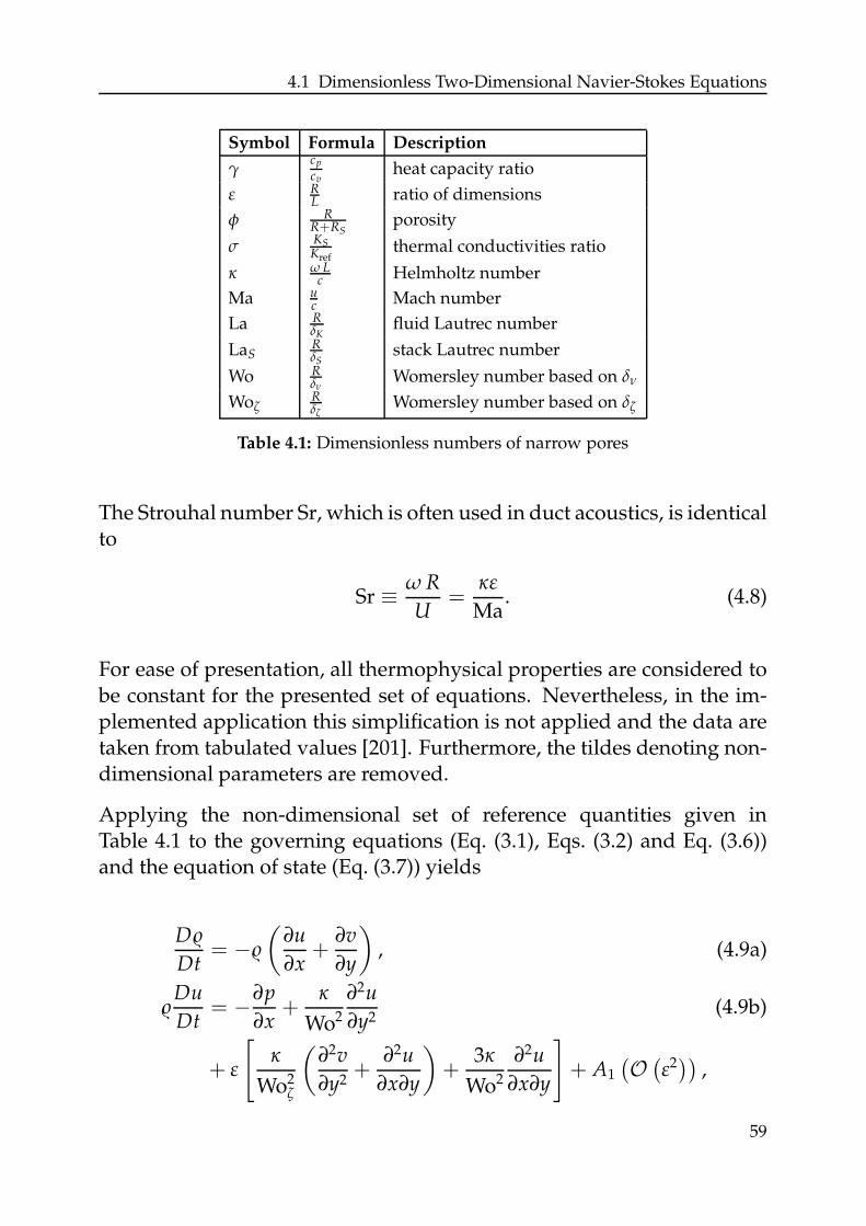
4.1 Dimensionless Two-Dimensional Navier-Stokes Equations
Symbol Formula Description
γcp
cvheat capacity ratio
ε RL ratio of dimensions
φ RR+RS
porosity
σ KSKref
thermal conductivities ratio
κ ω Lc Helmholtz number
Ma uc Mach number
La RδK
fluid Lautrec number
LaSRδS
stack Lautrec number
Wo Rδν
Womersley number based on δν
WoζRδζ
Womersley number based on δζ
Table 4.1: Dimensionless numbers of narrow pores
The Strouhal number Sr, which is often used in duct acoustics, is identicalto
Sr ≡ ω R
U=
κε
Ma. (4.8)
For ease of presentation, all thermophysical properties are considered tobe constant for the presented set of equations. Nevertheless, in the im-plemented application this simplification is not applied and the data aretaken from tabulated values [201]. Furthermore, the tildes denoting non-dimensional parameters are removed.
Applying the non-dimensional set of reference quantities given inTable 4.1 to the governing equations (Eq. (3.1), Eqs. (3.2) and Eq. (3.6))and the equation of state (Eq. (3.7)) yields
D
Dt= −
(∂u
∂x+
∂v
∂y
)
, (4.9a)
Du
Dt= −∂p
∂x+
κ
Wo2
∂2u
∂y2(4.9b)
+ ε
[
κ
Wo2ζ
(∂2v
∂y2+
∂2u
∂x∂y
)
+3κ
Wo2
∂2u
∂x∂y
]
+ A1
(O(ε2))
,
59
4 Inclusion of Mean Flow in Quasi 1D Thermoacoustic Transport Equations
0 = −∂p
∂y+ ε
κ
Wo2
∂2u
∂y2+ A2
(O(ε2))
, (4.9c)
DT
Dt= β T
Dp
Dt+
κ
2La2
∂2T
∂y2+
κ
Wo2
∂u
∂y
2
+ A3
(O(ε2))
, (4.9d)
p =γ − 1
γT . (4.9e)
In this formulation, the transversal momentum equation (Eq. (4.9c)) wasdivided by ε2 in order to obtain terms of order zero in ε.
Choosing an alternative coordinate system (x, yS) at the center of thesolid part (see Fig. 2.2) and RS as transversal parameter of non-dimensionalization, the porosity vanishes in the energy equation of thesolid:
S∂T
∂t=
κ
2La2S
∂2T
∂y2S
+ A4
(O(ε2))
. (4.9f)
Here, the terms Ai
(O(ε2))
contain higher-order contributions of the ra-tio of pore dimensions. In the following section, these quantities are ne-glected. Please refer to Section A.1 for further information on these terms.
The transversal boundary conditions for the geometric setup with con-stant pore cross-section are non-dimensionalized in the same way as thegoverning equations. For the velocity and temperature field they read
u(x, y = ±1) = 0, (4.10a)
v(x, y = ±1) = 0, (4.10b)
T(x, y = ±1) = TS(x, yS = ±1), (4.10c)
∂T
∂y
∣∣∣∣
y=±1
= σ∂TS
∂yS
∣∣∣∣
yS=±1
, (4.10d)
∂TS
∂yS
∣∣∣∣
yS=0
= 0. (4.10e)
4.2 Asymptotic Expansion
As stated in Section 3.2.1, carrying out an asymptotic expansion of thebasic set of equations assuming mean properties constant in time lead
60
4.2 Asymptotic Expansion
to the set of governing equations describing acoustic wave propagation.This technique is applied out in step II of the derivation depicted inFig. 4.1. Different expansion techniques can be found in literature. Thelinearization techniques applied in most TA publications are rather re-strictive [187], decomposing all transported scalars in terms of
Ψ(x, y, t) = Ψ0(x) +Re[Ψ1 (x, y) eiωt
]+ ... . (4.11)
This formulation only accounts for the values acquired during the mea-surement of acoustic quantities. Additionally, not considering the imagi-nary components in the resulting equations prohibits a stability analysisof any problem considered. The harmonic ansatz eiωt in time separatesacoustic oscillations from turbulent fluctuations. As the laminar regimeis treated, the latter magnitudes are estimated to be orders of magnitudessmaller than the acoustic counterpart.
Moreover, the expansion of the velocity vector v has no mean contribu-tion. Most authors justify this assumption by trying to suppress meanflow without providing any physical justification. In the present work,this limitation is removed by adopting a different approach. The zeroth-order quantity of v is only a function of the axial coordinate x. As longas mean flow is neglected, this approach is valid for inner pores witha mean temperature field that is not affected by multi-dimensional heatconduction effects due to heat transfer to the periphery.
The non-dimensionalization entails a transformation of the harmonicoscillation in time into the Helmholtz number (κ) space. The generalasymptotic expansion similar to Equation (3.9) then reads for an arbitraryvariable, i.e. the transport variables p, u, v, T, , but also the thermophys-ical properties of the solid and fluid region
Ψ(x, y, t) = Ψ0(x, y) + Maa Ψ1(x, y)eiκt
+ Maa2 (Ψ2,0(x, y) + Ψ2,1(x, y)e2iκt) +O(Maa
3). (4.12)
The first term scaling with Maa2 (index 0,2) is constant in time. It results
from the squared exponent of the complex valued frequency.
Thermophysical properties of fluids and solids are often assumed to beconstant. If this approach is too inaccurate for the considered problem,these quantities are computed as smooth functions of temperature and
61
4 Inclusion of Mean Flow in Quasi 1D Thermoacoustic Transport Equations
pressure (Section 3.1.5). As their relative change is always smaller thanthe change in the corresponding primary variables, all thermophysicalproperty contributions other than zeroth order are negligible. Thus, theyare considered as pure functions of the mean quantities, which in partic-ular leads to
β =1
T0(x, y)(4.13)
for the compressibility β of the gas.
In the present derivation, the asymptotic expansion is simplified furtherby assuming
Ψ0(x, y, t) = 〈Ψ0〉. (4.14)
The angle brackets of the right hand side term indicate a transversal av-erage over the channel height H
〈Ψ〉 = 2
H
H/2∫
0
Ψ(x, y) dy. (4.15)
This renders the mean quantities independent of the y-direction, which isonly valid for zero mean flow conditions. All preceding one-dimensionalmodels from Reid’s [158, 187] and in’t panhuis [80], which consider theimpact of mean flow follow the same approach for the mean flow quan-tities they take into account. The assumption of only considering meanparameters to be cross-sectionally constant is per se not physical and thusa modeling approach, which is necessary to keep the resulting system ofequations of the order of Maa manageable. Only if certain conditions ofcomparably negligible mean flow boundary layers arise in the problem,the error impact of the modeling approach is small.
The choice of this assumption causes the intermediate steps of the deriva-tion to be enhanced by one single parameter 〈u0〉(x) compared to thederivation of in’t panhuis [80]. mean velocity must be justified by phys-ical considerations: A comparison between the laminar velocity profilesinside a channel and the acoustic profiles of Rott’s solution (Eqs. (2.1))yields some insight into the interaction of acoustics and mean flow inthe thermoacoustic boundary layers. The mean velocity profiles u0(x, y)
62
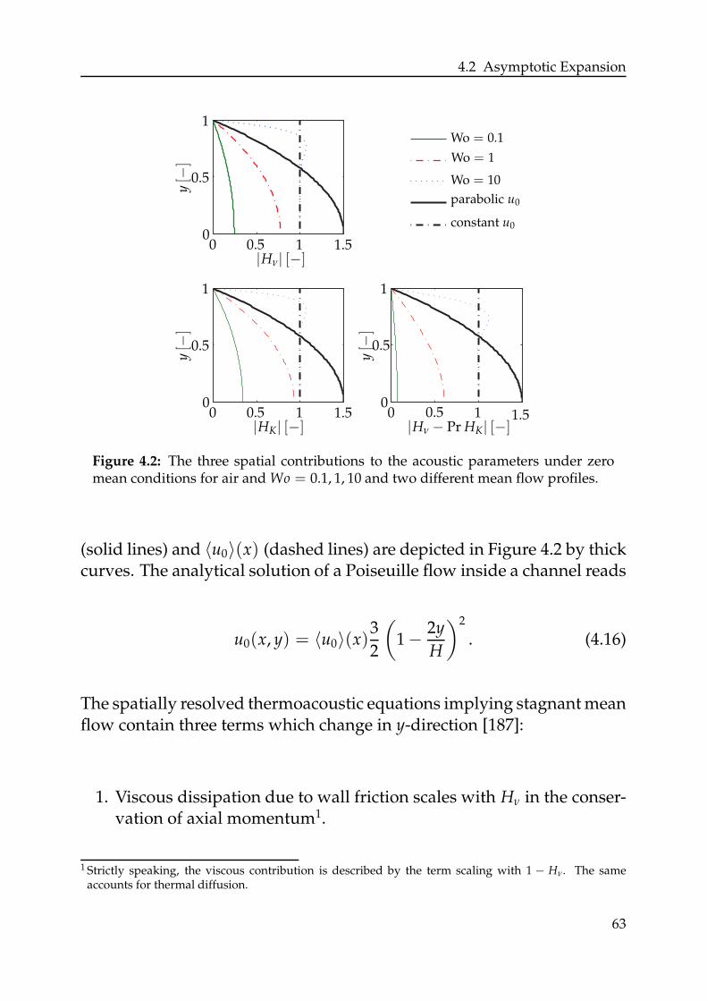
4.2 Asymptotic Expansion
00
00
00
1
1
1
1
1
1
0.5
0.5
0.5
0.5
1.5
1.5
0.5
0.5
1.5
Wo = 0.1
Wo = 1
Wo = 10
parabolic u0
constant u0
|Hν − Pr HK| [−]|HK| [−]
|Hν| [−]
y[−
]
y[−
]y[−
]
Figure 4.2: The three spatial contributions to the acoustic parameters under zeromean conditions for air and Wo = 0.1, 1, 10 and two different mean flow profiles.
(solid lines) and 〈u0〉(x) (dashed lines) are depicted in Figure 4.2 by thickcurves. The analytical solution of a Poiseuille flow inside a channel reads
u0(x, y) = 〈u0〉(x)3
2
(
1 − 2y
H
)2
. (4.16)
The spatially resolved thermoacoustic equations implying stagnant meanflow contain three terms which change in y-direction [187]:
1. Viscous dissipation due to wall friction scales with Hν in the conser-vation of axial momentum1.
1 Strictly speaking, the viscous contribution is described by the term scaling with 1 − Hν. The sameaccounts for thermal diffusion.
63
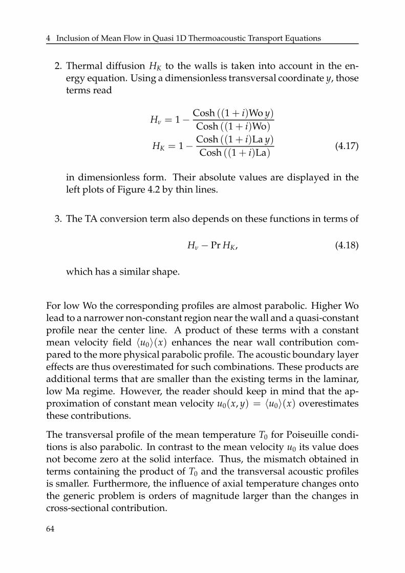
4 Inclusion of Mean Flow in Quasi 1D Thermoacoustic Transport Equations
2. Thermal diffusion HK to the walls is taken into account in the en-ergy equation. Using a dimensionless transversal coordinate y, thoseterms read
Hν = 1 − Cosh ((1 + i)Wo y)
Cosh ((1 + i)Wo)
HK = 1 − Cosh ((1 + i)La y)
Cosh ((1 + i)La)(4.17)
in dimensionless form. Their absolute values are displayed in theleft plots of Figure 4.2 by thin lines.
3. The TA conversion term also depends on these functions in terms of
Hν − Pr HK, (4.18)
which has a similar shape.
For low Wo the corresponding profiles are almost parabolic. Higher Wolead to a narrower non-constant region near the wall and a quasi-constantprofile near the center line. A product of these terms with a constantmean velocity field 〈u0〉(x) enhances the near wall contribution com-pared to the more physical parabolic profile. The acoustic boundary layereffects are thus overestimated for such combinations. These products areadditional terms that are smaller than the existing terms in the laminar,low Ma regime. However, the reader should keep in mind that the ap-proximation of constant mean velocity u0(x, y) = 〈u0〉(x) overestimatesthese contributions.
The transversal profile of the mean temperature T0 for Poiseuille condi-tions is also parabolic. In contrast to the mean velocity u0 its value doesnot become zero at the solid interface. Thus, the mismatch obtained interms containing the product of T0 and the transversal acoustic profilesis smaller. Furthermore, the influence of axial temperature changes ontothe generic problem is orders of magnitude larger than the changes incross-sectional contribution.
64
4.2 Asymptotic Expansion
4.2.1 Narrow Pore and Linear Acoustics Assumption
The full system of Equations (4.9) is a general formulation affected by thegeometrical ratio of dimensions of the pore
ε =R
L. (4.19)
If ε ≈ 1 and friction or thermal diffusion terms are of similar order, thefull system of equations needs to be considered. In contrast, in narrowpores with ε ≪ 1 as they occur in TA regenerators, these terms becomenegligible.
Acoustic quantities are generally of the order of [160]
Maa ≈p1
p0. 0.05. (4.20)
Thus, the terms scaling with either ε or Maa have a similar contributionin the expanded system of equations. Here, we follow Peter in’t panhuis[80], assuming
Maa ∼ ε2, (4.21)
which accounts for a low ratio of ε and linear acoustics. This approachyields a combined influence of geometric and acoustic streaming ef-fects in one system of equations of higher order, where combinations ofc0Maa
n + c1Maan−1ε + ... + cmMaa
n−mεm + ...cnεn balance. Findings basedon this system provide information about the impact of both parameters.
Applying Equation (4.21) and Equation (4.20) to the asymptotically ex-panded system of governing Equations ((4.9a)-(4.9e)), the system is sep-arated in groups of terms scaling with the order of Maa. As the zeroth-order group is time invariant and we consider the linear acoustic regime,the mean parameters have to fulfill the corresponding set of equations.Applying the same argument to the first-order terms directly yields alinearized system of equations describing the spatial and temporal evo-lution of acoustic parameters.
65
4 Inclusion of Mean Flow in Quasi 1D Thermoacoustic Transport Equations
4.3 Determination of Mean Field Quantities
The mean flow field is a set of temporally constant values providing back-ground information for the acoustic transport equations. It is the resultof step II of this derivation, the asymptotic expansion. With the chosenasymptotic expansion (3.9) and (4.14) , all transversal derivative termsbecome zero and the full system of equations describing mean transportprocesses reads
〈u0〉∂〈0〉
∂x= −〈0〉
∂〈u0〉∂x
, (4.22a)
〈0〉〈u0〉∂〈u0〉
∂x= −∂〈p0〉
∂x, (4.22b)
〈0〉〈u0〉∂〈T0〉
∂x= β 〈T0〉〈u0〉
∂〈p0〉∂x
, (4.22c)
〈p0〉 =γ − 1
γ〈T0〉 〈0〉. (4.22d)
The form of this system of equations is especially attributed to the cross-sectional means approach of (4.14). The cross-sectional average is onlyexact, if it is carried out for each term of the equations, e.g. the first term
of (4.22a) should read 〈u0∂0∂x 〉. Thus, Equation (4.22a) only accounts for
conditions of u0(x, y) = u0(x) or 0(x, y) = 0(x). The problems consid-ered here are always related to wall interaction. Unless the mean flowvelocity becomes zero, the contact condition leads to cross-sectional vari-ations in u0. Equation (4.9c) directly yields a constant pressure distribu-tion in this direction, hence
〈p0(x, y)〉 = p0(x). (4.23)
Thus, the ideal gas law (Eq. (4.9e)) states, that cross-sectional shape of0(x, y) is a function of the transversal mean temperature profile. Com-paring the spatial changes in these two quantities, the axial variation al-ways exceeds the transversal changes. Hence, this approach may be validunder certain conditions.
Under these assumptions, the transversal velocity component 〈v0〉 van-ishes, because the flow field is confined by the stack walls.
66
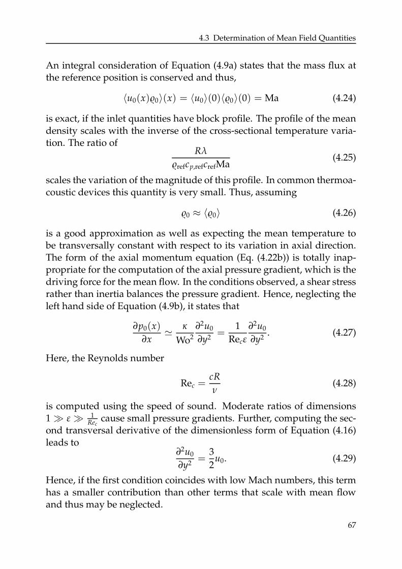
4.3 Determination of Mean Field Quantities
An integral consideration of Equation (4.9a) states that the mass flux atthe reference position is conserved and thus,
〈u0(x)0〉(x) = 〈u0〉(0)〈0〉(0) = Ma (4.24)
is exact, if the inlet quantities have block profile. The profile of the meandensity scales with the inverse of the cross-sectional temperature varia-tion. The ratio of
Rλ
refcp,refcrefMa(4.25)
scales the variation of the magnitude of this profile. In common thermoa-coustic devices this quantity is very small. Thus, assuming
0 ≈ 〈0〉 (4.26)
is a good approximation as well as expecting the mean temperature tobe transversally constant with respect to its variation in axial direction.The form of the axial momentum equation (Eq. (4.22b)) is totally inap-propriate for the computation of the axial pressure gradient, which is thedriving force for the mean flow. In the conditions observed, a shear stressrather than inertia balances the pressure gradient. Hence, neglecting theleft hand side of Equation (4.9b), it states that
∂p0(x)
∂x≃ κ
Wo2
∂2u0
∂y2=
1
Recε
∂2u0
∂y2. (4.27)
Here, the Reynolds number
Rec =cR
ν(4.28)
is computed using the speed of sound. Moderate ratios of dimensions1 ≫ ε ≫ 1
Reccause small pressure gradients. Further, computing the sec-
ond transversal derivative of the dimensionless form of Equation (4.16)leads to
∂2u0
∂y2=
3
2u0. (4.29)
Hence, if the first condition coincides with low Mach numbers, this termhas a smaller contribution than other terms that scale with mean flowand thus may be neglected.
67
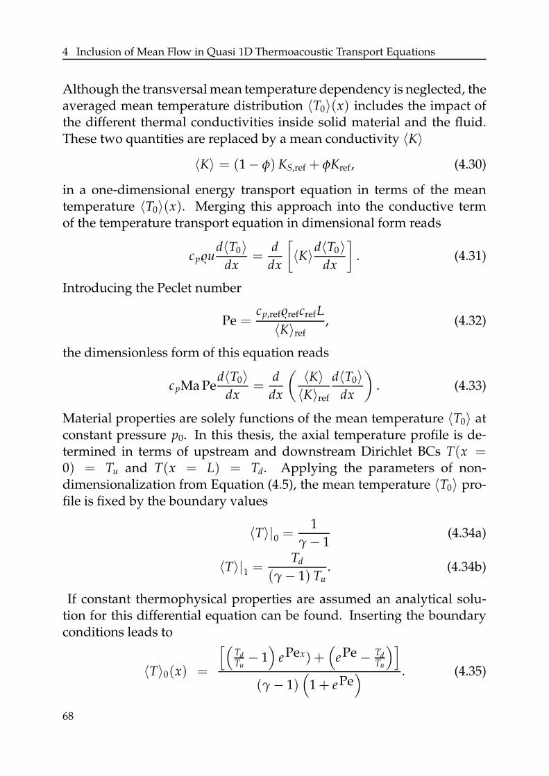
4 Inclusion of Mean Flow in Quasi 1D Thermoacoustic Transport Equations
Although the transversal mean temperature dependency is neglected, theaveraged mean temperature distribution 〈T0〉(x) includes the impact ofthe different thermal conductivities inside solid material and the fluid.These two quantities are replaced by a mean conductivity 〈K〉
〈K〉 = (1 − φ) KS,ref + φKref, (4.30)
in a one-dimensional energy transport equation in terms of the meantemperature 〈T0〉(x). Merging this approach into the conductive termof the temperature transport equation in dimensional form reads
cpud〈T0〉
dx=
d
dx
[
〈K〉d〈T0〉dx
]
. (4.31)
Introducing the Peclet number
Pe =cp,refrefcrefL
〈K〉ref, (4.32)
the dimensionless form of this equation reads
cpMa Ped〈T0〉
dx=
d
dx
( 〈K〉〈K〉ref
d〈T0〉dx
)
. (4.33)
Material properties are solely functions of the mean temperature 〈T0〉 atconstant pressure p0. In this thesis, the axial temperature profile is de-termined in terms of upstream and downstream Dirichlet BCs T(x =0) = Tu and T(x = L) = Td. Applying the parameters of non-dimensionalization from Equation (4.5), the mean temperature 〈T0〉 pro-file is fixed by the boundary values
〈T〉|0 =1
γ − 1(4.34a)
〈T〉|1 =Td
(γ − 1) Tu. (4.34b)
If constant thermophysical properties are assumed an analytical solu-tion for this differential equation can be found. Inserting the boundaryconditions leads to
〈T〉0(x) =
[(TdTu− 1)
ePex) +(
ePe − TdTu
)]
(γ − 1)(
1 + ePe) . (4.35)
68
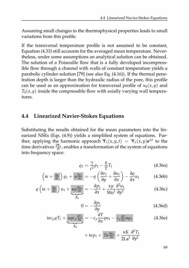
4.4 Linearized Navier-Stokes Equations
Assuming small changes in the thermophysical properties leads to smallvariations from this profile.
If the transversal temperature profile is not assumed to be constant,Equation (4.33) still accounts for the averaged mean temperature. Never-theless, under some assumptions an analytical solution can be obtained.The solution of a Poiseuille flow that is a fully developed incompress-ible flow through a channel with walls of constant temperature yields aparabolic cylinder solution [79] (see also Eq. (4.16)). If the thermal pene-tration depth is larger than the hydraulic radius of the pore, this profilecan be used as an approximation for transversal profile of u0(x, y) andT0(x, y) inside the compressible flow with axially varying wall tempera-tures.
4.4 Linearized Navier-Stokes Equations
Substituting the results obtained for the mean parameters into the lin-earized NSEs (Eqs. (4.9)) yields a simplified system of equations. Fur-ther, applying the harmonic approach Ψ1(x, y, t) = Ψ1(x, y)eiκt to thetime derivatives ∂Ψ1
∂t , enables a transformation of the system of equationsinto frequency space:
1 =γ
c2p1 −
TT1 (4.36a)
(
iκ + ∂u∂x
)
1 + u∂1∂x = −
(∂v1
∂y+
∂u1
∂x
)
− ∂
∂xu1 (4.36b)
(
iκ + ∂u∂x
)
u1 + u ∂u1∂x
︸ ︷︷ ︸
Λ1
= −∂p1
∂x+
κµ
Wo2
∂2u1
∂y2(4.36c)
0 = −∂p1
∂y(4.36d)
iκcpT1 + ucp∂T1∂x
︸ ︷︷ ︸
Λ2
= −cp∂T
∂xu1 − cp
∂T∂x
u1 (4.36e)
+ iκp1 + Tu∂p1∂x +
κK
2La2
∂2T1
∂y2
69
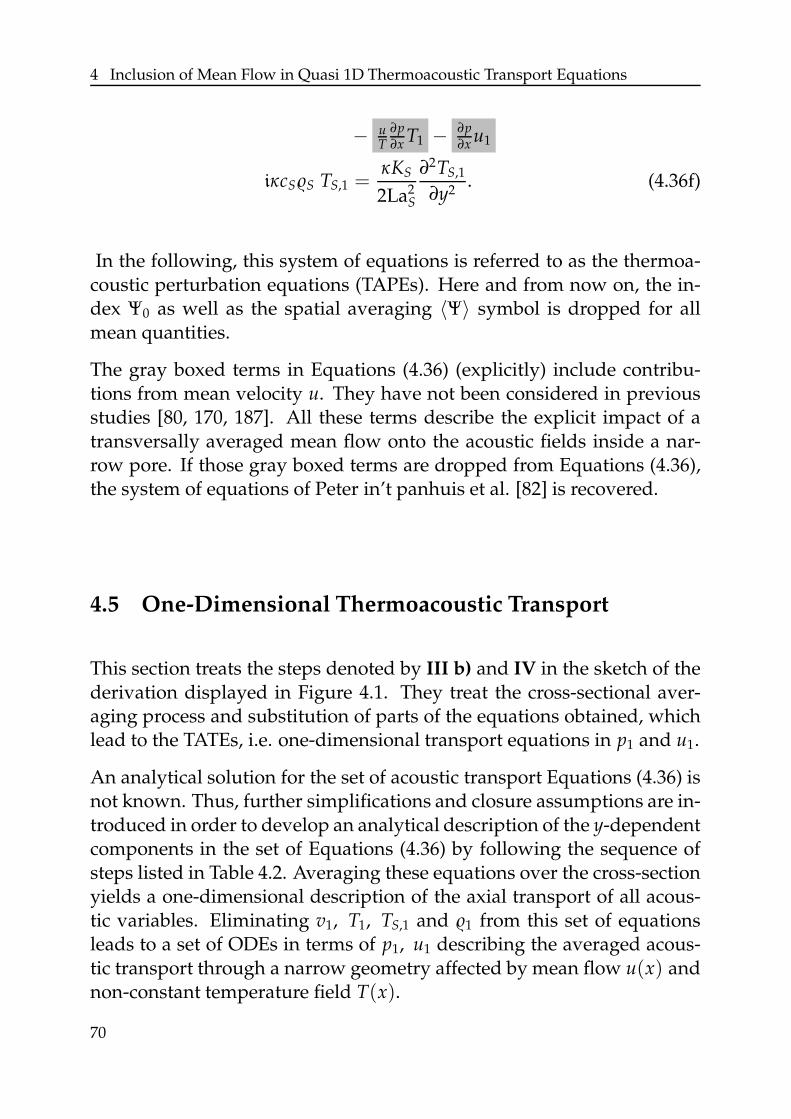
4 Inclusion of Mean Flow in Quasi 1D Thermoacoustic Transport Equations
− uT
∂p∂x
T1 − ∂p∂x
u1
iκcSS TS,1 =κKS
2La2S
∂2TS,1
∂y2. (4.36f)
In the following, this system of equations is referred to as the thermoa-coustic perturbation equations (TAPEs). Here and from now on, the in-dex Ψ0 as well as the spatial averaging 〈Ψ〉 symbol is dropped for allmean quantities.
The gray boxed terms in Equations (4.36) (explicitly) include contribu-tions from mean velocity u. They have not been considered in previousstudies [80, 170, 187]. All these terms describe the explicit impact of atransversally averaged mean flow onto the acoustic fields inside a nar-row pore. If those gray boxed terms are dropped from Equations (4.36),the system of equations of Peter in’t panhuis et al. [82] is recovered.
4.5 One-Dimensional Thermoacoustic Transport
This section treats the steps denoted by III b) and IV in the sketch of thederivation displayed in Figure 4.1. They treat the cross-sectional aver-aging process and substitution of parts of the equations obtained, whichlead to the TATEs, i.e. one-dimensional transport equations in p1 and u1.
An analytical solution for the set of acoustic transport Equations (4.36) isnot known. Thus, further simplifications and closure assumptions are in-troduced in order to develop an analytical description of the y-dependentcomponents in the set of Equations (4.36) by following the sequence ofsteps listed in Table 4.2. Averaging these equations over the cross-sectionyields a one-dimensional description of the axial transport of all acous-tic variables. Eliminating v1, T1, TS,1 and 1 from this set of equationsleads to a set of ODEs in terms of p1, u1 describing the averaged acous-tic transport through a narrow geometry affected by mean flow u(x) andnon-constant temperature field T(x).
70
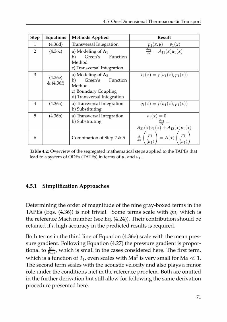
4.5 One-Dimensional Thermoacoustic Transport
Step Equations Methods Applied Result
1 (4.36d) Transversal Integration p1(x, y) = p1(x)
2 (4.36c) a) Modeling of Λ1
b) Green’s FunctionMethodc) Transversal Integration
∂p1∂x = A11(x)u1(x)
3(4.36e)
& (4.36f)
a) Modeling of Λ2
b) Green’s FunctionMethodc) Boundary Couplingd) Transversal Integration
T1(x) = f (u1(x), p1(x))
4 (4.36a) a) Transversal Integrationb) Substituting
1(x) = f (u1(x), p1(x))
5 (4.36b) a) Transversal Integrationb) Substituting
v1(x) = 0∂u1∂x =
A21(x)u1(x) + A12(x)p1(x)
6 Combination of Step 2 & 5 ddx
(
p1
〈u1〉
)
= A(x)
(
p1
〈u1〉
)
Table 4.2: Overview of the segregated mathematical steps applied to the TAPEs thatlead to a system of ODEs (TATEs) in terms of p1 and u1 .
4.5.1 Simplification Approaches
Determining the order of magnitude of the nine gray-boxed terms in theTAPEs (Eqs. (4.36)) is not trivial. Some terms scale with u, which isthe reference Mach number (see Eq. (4.24)). Their contribution should beretained if a high accuracy in the predicted results is required.
Both terms in the third line of Equation (4.36e) scale with the mean pres-sure gradient. Following Equation (4.27) the pressure gradient is propor-tional to Ma
Recε, which is small in the cases considered here. The first term,
which is a function of T1, even scales with Ma2 is very small for Ma ≪ 1.The second term scales with the acoustic velocity and also plays a minorrole under the conditions met in the reference problem. Both are omittedin the further derivation but still allow for following the same derivationprocedure presented here.
71
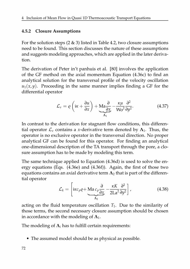
4 Inclusion of Mean Flow in Quasi 1D Thermoacoustic Transport Equations
4.5.2 Closure Assumptions
For the solution steps (2 & 3) listed in Table 4.2, two closure assumptionsneed to be found. This section discusses the nature of these assumptionsand suggests modeling approaches, which are applied in the later deriva-tion.
The derivation of Peter in’t panhuis et al. [80] involves the applicationof the GF method on the axial momentum Equation (4.36c) to find ananalytical solution for the transversal profile of the velocity oscillationu1(x, y). Proceeding in the same manner implies finding a GF for thedifferential operator
Lν =
(
iκ +∂u
∂x
)
+ Ma∂
∂x︸ ︷︷ ︸
Λ1
− κµ
Wo2
∂2
∂y2. (4.37)
In contrast to the derivation for stagnant flow conditions, this differen-tial operator Lν contains a x-derivative term denoted by Λ1. Thus, theoperator is no exclusive operator in the transversal direction. No properanalytical GF can be found for this operator. For finding an analyticalone-dimensional description of the TA transport through the pore, a clo-sure assumption has to be made by modeling this term.
The same technique applied to Equation (4.36d) is used to solve the en-ergy equations (Eqs. (4.36e) and (4.36f)). Again, the first of those twoequations contains an axial derivative term Λ2 that is part of the differen-tial operator
Lk =
[
iκcp+Ma cp∂
∂x︸ ︷︷ ︸
Λ2
− κK
2La2
∂2
∂y2
]
, (4.38)
acting on the fluid temperature oscillation T1. Due to the similarity ofthose terms, the second necessary closure assumption should be chosenin accordance with the modeling of Λ1.
The modeling of Λi has to fulfill certain requirements:
• The assumed model should be as physical as possible.
72
4.5 One-Dimensional Thermoacoustic Transport
Term Character Model
MI MII
∂u1∂x Λ1 0 ∂〈u1〉
∂x
∣∣∣u0=0
∂T1∂x Λ2 0 ∂〈T1〉
∂x
∣∣∣u0=0
Table 4.3: Overview over the modeled terms. Choosing different closure assump-tions leads to different results in the one-dimensional transport equations (MI, MII).
• The basic shape of the GF for the Li considered should not be dom-inated by the modeled term. Thus, if parts of the model contributeto LiΨ1, they should be formulated in terms of Ψ1 and its second
transversal derivative ∂2Ψ1
∂y2 .
• Such model terms do not have to be constant in y but their mathe-matical formulation should lead to an analytical GF.
• The y-profile of the source terms has to be known beforeEquation (3.54) can be applied to find an analytical solution. There-fore, the transversal evolution of all contributions that do not includethe sought variable Ψ should be given.
With these restrictions, two different basic assumptions can be found tomodel the closure terms in a first step:
MI: As the terms Λi scale with Ma, their contribution can be neglectedand both terms vanish. This approach keeps the resulting system ofequations short. However, this approach is not consistent, becauseother mean flow terms in Equation (4.36) also scale with Ma.
MII: The analytical solution for stagnant mean conditions is known. Asthis thesis deals with laminar mean flow conditions, the low velocitylimit is described by these equations. The accuracy of this approachis estimated to decrease in the same way as the first approach. Thisinitial approach is simplified here, such that only a transversally av-eraged version of the terms is applied.
Iteratively substituting the results of these approaches may lead to moreaccurate results unless an intermediate solution does not fulfill the re-
73
4 Inclusion of Mean Flow in Quasi 1D Thermoacoustic Transport Equations
quirements stated before. The mathematical formulation for the terms Λi
of these two models are gathered in Table 4.3.
Using these closure assumptions, an analytical solution may be obtainedfrom Equations (4.36). To keep the derivation more general, the termsare not explicitly substituted, but replaced by two placeholders Λi in thederivation in the next section.
4.5.3 Spatial Averaging of the TAPEs
Here, the cross-sectional averaging of the system of Equations (4.36) istreated. Due to the huge amount of terms that occur in this process, thepertinent terminology is briefly explained. The blackboard bold capitalletters (e.g. E) indicate the equation into which the replacement characteris introduced. The overbar (Φ) marks the terms stemming from transver-sally averaged equations. The indices refer to different issues. They ei-ther indicate the corresponding prefactors the term multiplies with (e.g.p1) or stand for specially included parameters. The latter are for examplethe cross-sectional impact functions Fν, FK or the modeled closure terms(Λi). Table 4.4 lists the abbreviations and indices and offers a referenceto the corresponding equations. All terms are defined and related to thecorresponding equations in Section A.2. The cross-sectional averaging ofthe parameter u1, T1 and 1 is processed by applying Equation (4.15) tothe analytical definition obtained for the quantities.
A brief look at the transversal momentum conservation (Eq. (4.36d)) re-veals that not only the mean pressure field is constant over the cross-section of the channel, but also the acoustic pressure p1(x, y) = p1(x)(step 1 in Tab. 4.2).
Merging the closure assumptions of the last section into the y-momentumEquation (4.36c) and using the differential operator of Equation (4.37)facilitates rewriting the acoustic velocity problem as
Lν [u1] = XΛ1+ Xp′1
∂p1
∂x, (4.39)
u1
∣∣±1
= 0. (4.40)
74
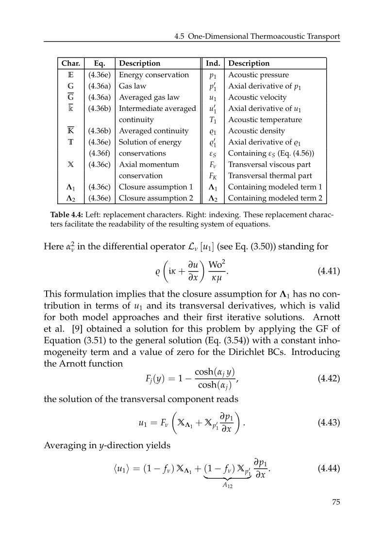
4.5 One-Dimensional Thermoacoustic Transport
Char. Eq. Description Ind. Description
E (4.36e) Energy conservation p1 Acoustic pressure
G (4.36a) Gas law p′1 Axial derivative of p1
G (4.36a) Averaged gas law u1 Acoustic velocity
k (4.36b) Intermediate averaged u′1 Axial derivative of u1
continuity T1 Acoustic temperature
K (4.36b) Averaged continuity 1 Acoustic density
T (4.36e) Solution of energy ′1 Axial derivative of 1
(4.36f) conservations εS Containing εS (Eq. (4.56))
X (4.36c) Axial momentum Fν Transversal viscous part
conservation FK Transversal thermal part
Λ1 (4.36c) Closure assumption 1 Λ1 Containing modeled term 1
Λ2 (4.36e) Closure assumption 2 Λ2 Containing modeled term 2
Table 4.4: Left: replacement characters. Right: indexing. These replacement charac-ters facilitate the readability of the resulting system of equations.
Here α2ν in the differential operator Lν [u1] (see Eq. (3.50)) standing for
(
iκ +∂u
∂x
)Wo2
κµ. (4.41)
This formulation implies that the closure assumption for Λ1 has no con-tribution in terms of u1 and its transversal derivatives, which is validfor both model approaches and their first iterative solutions. Arnottet al. [9] obtained a solution for this problem by applying the GF ofEquation (3.51) to the general solution (Eq. (3.54)) with a constant inho-mogeneity term and a value of zero for the Dirichlet BCs. Introducingthe Arnott function
Fj(y) = 1 − cosh(αj y)
cosh(αj), (4.42)
the solution of the transversal component reads
u1 = Fν
(
XΛ1+ Xp′1
∂p1
∂x
)
. (4.43)
Averaging in y-direction yields
〈u1〉 = (1 − fν)XΛ1+ (1 − fν)Xp′1︸ ︷︷ ︸
A12
∂p1
∂x. (4.44)
75
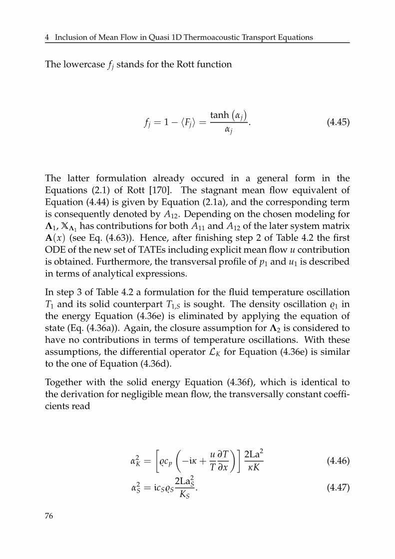
4 Inclusion of Mean Flow in Quasi 1D Thermoacoustic Transport Equations
The lowercase f j stands for the Rott function
f j = 1 − 〈Fj〉 =tanh
(αj
)
αj. (4.45)
The latter formulation already occured in a general form in theEquations (2.1) of Rott [170]. The stagnant mean flow equivalent ofEquation (4.44) is given by Equation (2.1a), and the corresponding termis consequently denoted by A12. Depending on the chosen modeling forΛ1, XΛ1
has contributions for both A11 and A12 of the later system matrixA(x) (see Eq. (4.63)). Hence, after finishing step 2 of Table 4.2 the firstODE of the new set of TATEs including explicit mean flow u contributionis obtained. Furthermore, the transversal profile of p1 and u1 is describedin terms of analytical expressions.
In step 3 of Table 4.2 a formulation for the fluid temperature oscillationT1 and its solid counterpart T1,S is sought. The density oscillation 1 inthe energy Equation (4.36e) is eliminated by applying the equation ofstate (Eq. (4.36a)). Again, the closure assumption for Λ2 is considered tohave no contributions in terms of temperature oscillations. With theseassumptions, the differential operator LK for Equation (4.36e) is similarto the one of Equation (4.36d).
Together with the solid energy Equation (4.36f), which is identical tothe derivation for negligible mean flow, the transversally constant coeffi-cients read
α2K =
[
cp
(
−iκ +u
T
∂T
∂x
)]2La2
κK(4.46)
α2S = icSS
2La2S
KS. (4.47)
76
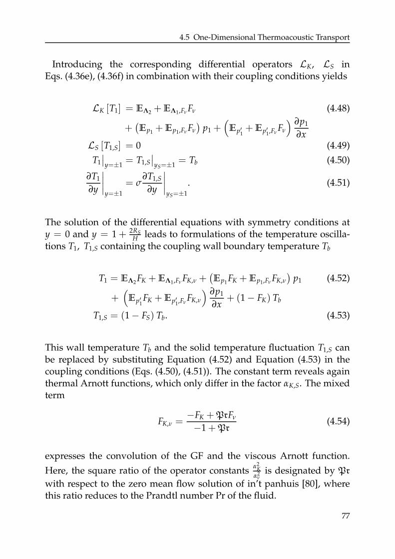
4.5 One-Dimensional Thermoacoustic Transport
Introducing the corresponding differential operators LK, LS inEqs. (4.36e), (4.36f) in combination with their coupling conditions yields
LK [T1] = EΛ2+ EΛ1,Fν Fν (4.48)
+(Ep1
+ Ep1,Fν Fν
)p1 +
(
Ep′1+ Ep′1,Fν
Fν
) ∂p1
∂xLS [T1,S] = 0 (4.49)
T1
∣∣
y=±1= T1,S
∣∣
yS=±1= Tb (4.50)
∂T1
∂y
∣∣∣∣
y=±1
= σ∂T1,S
∂y
∣∣∣∣
yS=±1
. (4.51)
The solution of the differential equations with symmetry conditions aty = 0 and y = 1 + 2RS
Hleads to formulations of the temperature oscilla-
tions T1, T1,S containing the coupling wall boundary temperature Tb
T1 = EΛ2FK + EΛ1,Fν FK,ν +
(Ep1
FK + Ep1,Fν FK,ν
)p1 (4.52)
+(
Ep′1FK + Ep′1,Fν
FK,ν
) ∂p1
∂x+ (1 − FK) Tb
T1,S = (1 − FS) Tb. (4.53)
This wall temperature Tb and the solid temperature fluctuation T1,S canbe replaced by substituting Equation (4.52) and Equation (4.53) in thecoupling conditions (Eqs. (4.50), (4.51)). The constant term reveals againthermal Arnott functions, which only differ in the factor αK,S. The mixedterm
FK,ν =−FK +PrFν
−1 +Pr(4.54)
expresses the convolution of the GF and the viscous Arnott function.
Here, the square ratio of the operator constantsα2
K
α2ν
is designated by Pr
with respect to the zero mean flow solution of in’t panhuis [80], wherethis ratio reduces to the Prandtl number Pr of the fluid.
77
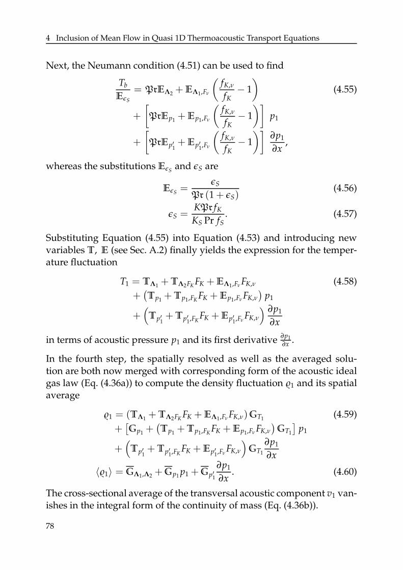
4 Inclusion of Mean Flow in Quasi 1D Thermoacoustic Transport Equations
Next, the Neumann condition (4.51) can be used to find
Tb
EǫS
= PrEΛ2+ EΛ1,Fν
(fK,ν
fK− 1
)
(4.55)
+
[
PrEp1+ Ep1,Fν
(fK,ν
fK− 1
)]
p1
+
[
PrEp′1+ Ep′1,Fν
(fK,ν
fK− 1
)]∂p1
∂x,
whereas the substitutions EǫSand ǫS are
EǫS=
ǫS
Pr (1 + ǫS)(4.56)
ǫS =KPr fK
KS Pr fS. (4.57)
Substituting Equation (4.55) into Equation (4.53) and introducing newvariables T, E (see Sec. A.2) finally yields the expression for the temper-ature fluctuation
T1 = TΛ1+ TΛ2FK
FK + EΛ1,Fν FK,ν (4.58)
+(Tp1
+ Tp1,FKFK + Ep1,Fν FK,ν
)p1
+(
Tp′1+ Tp′1,FK
FK + Ep′1,FνFK,ν
) ∂p1
∂x
in terms of acoustic pressure p1 and its first derivative ∂p1∂x .
In the fourth step, the spatially resolved as well as the averaged solu-tion are both now merged with corresponding form of the acoustic idealgas law (Eq. (4.36a)) to compute the density fluctuation 1 and its spatialaverage
1 = (TΛ1+ TΛ2FK
FK + EΛ1,Fν FK,ν)GT1(4.59)
+[Gp1
+(Tp1
+ Tp1,FKFK + Ep1,Fν FK,ν
)GT1
]p1
+(
Tp′1+ Tp′1,FK
FK + Ep′1,FνFK,ν
)
GT1
∂p1
∂x
〈1〉 = GΛ1,Λ2+ Gp1
p1 + Gp′1
∂p1
∂x. (4.60)
The cross-sectional average of the transversal acoustic component v1 van-ishes in the integral form of the continuity of mass (Eq. (4.36b)).
78
4.5 One-Dimensional Thermoacoustic Transport
Substituting the density and its axial derivative and replacing ∂p1/∂x in
∂ 〈u1〉∂x
= KΛ1,Λ2+ Kp1
p1 + Kp′1
∂p1
∂x+ Ku1
〈u1〉 (4.61)
by Equation (4.44) (step 6) finally leads to the second TATE
∂ 〈u1〉∂x
= KΛ1,Λ2−
Kp′1XΛ1
Xp′1
+ Kp1
︸ ︷︷ ︸
A21
p1 +
[
Ku1+
Kp′1
(1 − fν)Xp′1
]
︸ ︷︷ ︸
A22
〈u1〉 .
(4.62)
It describes the axial propagation of the acoustic variables p1, u1. Again,its stagnant mean flow equivalent formulation is given by Equation (2.1b)in Section 2.1. As in the first TATE (Eq. (4.44)), the corresponding matrixentries are marked by A21 and A22. Here, first two terms show the impactof both closure terms Λ1,2. Assuming a description of those two modelingapproaches in terms of u1 and p1, the system of ODEs reads
d
dx
(
p1
〈u1〉
)
= A(x)
(
p1
〈u1〉
)
. (4.63)
All three quasi one-dimensional models investigated in Chapters 7 and 8can be drawn from this system of equations. Assuming zero contributionof mean flow (IMP), all gray-boxed terms in the TAPEs (Eqs. (4.36)) van-ish. If the terms Λ1,2 are neglected (MI), all terms indexed correspond-ingly do not contribute to the system. Finally, for MII contributions ofthese terms occur in various steps of the derivation process, such thatthey affect all the four matrix entries in Equation (4.63).
4.5.4 Achieving High Modeling Accuracy
The derivation presented in the last section contains some simplificationsthat are not imperative for achieving an analytical system of differentialequations. A more general version always leads to more complex results.Moreover, dropping two or more of these simplifications leads – espe-cially due to the convolution of the right-hand side terms in steps 2 & 3 –
79
4 Inclusion of Mean Flow in Quasi 1D Thermoacoustic Transport Equations
to a combination of these terms that cause an immense increase in com-plexity of some of the resulting terms. Thus, in the following sections,ideas for improving the physical description of the transport equationsare presented separately. The reader should be aware of the possibility ofcombining some of the improvements.
4.5.4.1 Parabolic Mean Distribution
As stated in Section 4.3, an analytical solution of a laminar profile of acompressible fluid through a channel with non-isothermal walls is notknown. Thus, a quadratic isothermal transversal profile is assumed forthe mean velocity. Keeping the averaged value 〈u0〉(x) as scaling param-eter, the mean velocity follows Equation (4.16). Applying this approachinto the mass conservation (Eq. (4.9a)) yields a similar profile for meandensity and temperature. Following the arguments of Section 4.2, thisvariation is less drastic and can be neglected in a first approach. Ap-plying this mean distribution only to the right-hand side terms is notconsistent.
If the parabolic shape of the mean velocity is only taken into account forinhomogeneities on the right-hand side of Equations (4.36c) and (4.36e),these terms are not constant. Hence their convolution with the originalGF yields
1∫
0
(1 − y2)G(y, y)dy =
+
(
α2j − 2
)
sinh(yαj) + 4 sinh((1 + y)αj) +(
α2j − 2
)
sinh((2 + y)αj))
4α2j cosh(αj) sinh(αj)
+(2 +
(y2 − 1
)α2
j − 2 cosh(αj − yαj) + 2αj sinh(αj − yαj))
α2j
H(−1 + y)
−
(
2 +(y2 − 1
)α2
j +(
α2j − 2
)
cosh(yαj))
α2j
H(y). (4.64)
This expression including the Heaviside function H(y) does not simplifysignificantly by applying the cross-sectional averaging. This expansion
80
4.5 One-Dimensional Thermoacoustic Transport
increases the number of terms and computational costs by a factor oftwo.
The velocity profile also couples with the density fluctuation in the con-servation of mass (Eq. (4.36b)). Thus, especially the pressure trans-port equation equivalent of Equation (4.62) is affected by changes in thetransversal mean velocity profile u(y).
Nevertheless, if u is a function of the y-direction, the problem specific GFchanges as well. Applying a coordinate transformation, the differentialoperator of the axial momentum Equation (4.36c) reads
[(C − y2
)− ∂2
∂y2
]
u1(x, y). (4.65)
C represents a constant consisting of various terms. The solution of sucha system of equations is an integral combination of Gamma functionsΓ(y) and Weber W(y) functions with complex-valued arguments of dif-ferent magnitudes. Due to this integral form, deriving these equationsgoes beyond the scope of this thesis and is not presented here.
In general, integral solutions increase the computational effort comparedto the determination of one of the hyperbolic functions of the solutionsin Section 4.5.
Furthermore, the interaction of hydraulic and thermal y-profile, whichleads to FK,ν in Equation (4.52), has an extra parabolic contribution term.It originates from the substituted conservation of mass (Eq. (4.36b)). Theconvolution results in an equation that is too large to display in this con-text.
Summarizing, taking additionally the transversal density and tempera-ture evolution into account leads to an enormous complexity in the sys-tem.
4.5.4.2 Spatially Distributed Modeling Terms
In Section 4.5.2, MII was simplified by substituting the averaged form ofthe stagnant mean solution instead of the y-dependent form. Originally,
81
4 Inclusion of Mean Flow in Quasi 1D Thermoacoustic Transport Equations
the right-hand side term replaced by Λ1 is a function of αj,q, the L termof Equation (3.50) scaling the Arnott function and the y-coordinate.
Introducing the inhomogeneity
b(y) = 1 − cosh(αj,qy
)
cosh(
1αj,q
) (4.66)
in Equation (3.54) and averaging in cross-sectional direction yields
1∫
0
1∫
0
b(y)G(y, y)dydy = (4.67)
1
2(1 + exp(αj
))(1 + exp(2αj))αj,qαj(−αj,q + αj)(αj,q + αj)
[
(exp(αj
)− 1)(1 + exp(2αj))αj,qα2
j sinh−1 (αj,q
)
+ αj,q
[
(1 + exp(2αj))α2j (1 + 2αj + exp
(αj
)(−1 + 2αj))
− α2j,q
(3 + 2αj + exp(2αj)
[1 + 2αj + 4(−1 + αj) cosh
(αj
)− 2 sinh
(αj
)])]
− 2(1 + exp(αj
))(1 + exp(2αj))α
3j tanh
(αj,q
)
]
.
Compared to the resulting transport equation stemming from the mo-mentum Equation (4.36c) using MI or MII, respectively, leads to an enor-mous increase in terms. These again have to be considered in the con-volution of the right-hand side terms of the energy Equation (4.36e). Asthis integration is straightforward, the solution can be sought, but thecomputational costs increase immensely. This improvement in analyticaldescription further comes along with a higher complexity of the systemof equations, which are prone to implementation errors and numericalaccuracy.
A comparison to two-dimensional computations might still yield advan-tages for the computing time of the one dimensional set, but the complex-ity of the system implies a high error rate for the implementation and alow accuracy due to numerical errors occurring because of the numerousterms.
82
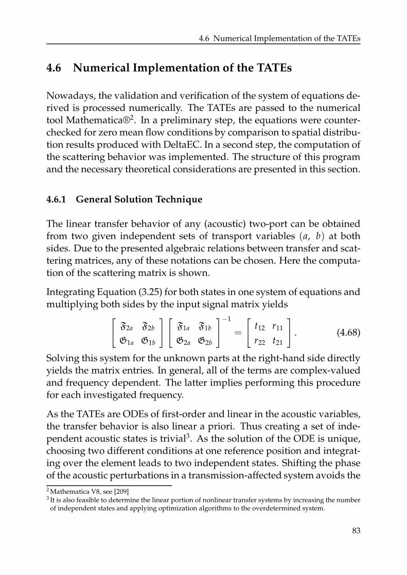
4.6 Numerical Implementation of the TATEs
4.6 Numerical Implementation of the TATEs
Nowadays, the validation and verification of the system of equations de-rived is processed numerically. The TATEs are passed to the numericaltool Mathematica®2. In a preliminary step, the equations were counter-checked for zero mean flow conditions by comparison to spatial distribu-tion results produced with DeltaEC. In a second step, the computation ofthe scattering behavior was implemented. The structure of this programand the necessary theoretical considerations are presented in this section.
4.6.1 General Solution Technique
The linear transfer behavior of any (acoustic) two-port can be obtainedfrom two given independent sets of transport variables (a, b) at bothsides. Due to the presented algebraic relations between transfer and scat-tering matrices, any of these notations can be chosen. Here the computa-tion of the scattering matrix is shown.
Integrating Equation (3.25) for both states in one system of equations andmultiplying both sides by the input signal matrix yields
[
F2a F2b
G1a G1b
] [
F1a F1b
G2a G2b
]−1
=
[
t12 r11
r22 t21
]
. (4.68)
Solving this system for the unknown parts at the right-hand side directlyyields the matrix entries. In general, all of the terms are complex-valuedand frequency dependent. The latter implies performing this procedurefor each investigated frequency.
As the TATEs are ODEs of first-order and linear in the acoustic variables,the transfer behavior is also linear a priori. Thus creating a set of inde-pendent acoustic states is trivial3. As the solution of the ODE is unique,choosing two different conditions at one reference position and integrat-ing over the element leads to two independent states. Shifting the phaseof the acoustic perturbations in a transmission-affected system avoids the
2 Mathematica V8, see [209]3 It is also feasible to determine the linear portion of nonlinear transfer systems by increasing the number
of independent states and applying optimization algorithms to the overdetermined system.
83
4 Inclusion of Mean Flow in Quasi 1D Thermoacoustic Transport Equations
problem of a determinant of the input signal matrix to become zero whichmight occur for randomly chosen conditions. Therefore the conditionsat x = 0 are determined as follows. The amplitudes of acoustic pres-sure |p1|a/b/c and velocity |u1|a/b are set to unity. In order to cause thestates to be independent, their relative phases are set to φa(u1, p1) = 0and φb(u1, p1) = π respectively.
4.6.2 Implementation
Before the TATEs can be solved numerically, the mean temperature dis-tribution is computed from equation (4.33) for given reference tempera-tures at the hot and cold end using a shooting method [154]. For com-putational reasons, the solution is interpolated with second-order accu-racy from stored tabulated data. As can be seen from Appendix A.2, thehighest-order derivative of the mean temperature is ∂2T0/∂x2, which jus-tifies this approach.
Within a given mean temperature distribution, the TATE system is inte-grated from the cold reference end to the hot side of the pore. A standardAdams-Bashforth [154] integration scheme with an accuracy of 10−12 isused in combination of a maximum step size of 10−6, which revealedparameter-independent results for the test cases presented in the follow-ing.
4.7 Advantages and Drawbacks of Mean Flow Inclusion
The system of equations derived in this chapter contains formulationsthat explicitly contain mean flow in terms of 〈u0〉. Such a set is denotedexplicit in contrast to the Equations (2.1) of Rott [170] and Swift [187].These TATEs of the IMP model are only affected by a mean flow con-trolled temperature profile T0(x) = f (〈u0〉(x)) and thus couple implicitlywith 〈u0〉(x).As stated in Section 2.1, these implicit equations are physical for stagnantmean flow conditions in narrow pore geometries [80]. The Rott func-tions for various geometries have been derived [187] and even arbitrary
84
4.7 Advantages and Drawbacks of Mean Flow Inclusion
shapes are conceivable [105]. Some of these findings may be adapted tothe system of transport equations derived. As closure terms are used inthe derivation of the TATEs, the system of equations is an approximationof the actual physics. The validity of a direct adaption of the Rott func-tions for geometries other than the 2D channel by adjusting the α valueof the differential operator is yet to be proven. However, the small dif-ferences in the shape of the Rott functions [187] and especially in theirinstability potentiality [72] facilitate a comparison of the results obtainedfor different pore geometries with good accuracy.
The accuracy of the explicit TATEs (Eqs. (4.63)) for the basic closure as-sumptions is partially demonstrated in Chapter 8. Especially the im-provement over the implicit Equations (2.1) is clearly visible from theinvestigated cases. Nevertheless, future investigations are needed to con-firm these observations for other cases.
Due to the numerous additional terms of the explicit TATEs (Eqs. (4.63)),the computational costs for the prediction of the scattering behavior in-creases with every iteration for the closure assumption. Tests showedthat the computational time for one single evolution of the acoustic pres-sure and velocity was almost tripled for MI and fifteen times larger forMII. Using high-order interpolation and tabulated values for the prefac-tors of the TATEs (Eqs. (4.63)), for the computation of scattering matrices,should reduce this additional effort.
The complexity of the TATEs makes a physical interpretation of the differ-ent terms harder. In the implicit equations, the influence of viscous dissi-pation, thermal diffusion and the interaction leading to energy transfer isstill visible. This is not true for the explicit TATEs. The convective terms,i.e. terms that have mean flow contribution, mix the latter two compo-nents and yield less physical insight. This effect is not based on the mod-eling approaches, but on the physics of the problem. Hence modelingthe closure terms implies a cautious validation of the approaches. Theseconsiderations demonstrate that these explicit TATEs (Eqs. (4.63)) shouldbe used with care. Improved accuracy requires increased computationalcosts. Finding a reasonable balance depends on the problem consideredand demanded error limits.
85

4 Inclusion of Mean Flow in Quasi 1D Thermoacoustic Transport Equations
86
5 CFD/SI - Time Domain Analysis of Thermoa-coustic Scattering
Determining the frequency response of a certain acoustic problem setupusing a combination of transient CFD simulations and system identifi-cation (SI) methods is a central issue of various research activities at theLehrstuhl fur Thermodynamik at the TU Munchen [57, 63, 75, 88, 95, 192,200]. The basic technique, which originates from system theory and sig-nal processing, was adapted to acoustic SISO1 problems by Polifke et al.[146] and Gentemann et al. [62]. The idea is to reconstruct the frequency-dependent transfer function by determining the unit impulse responsefrom the time series of the in- and output signals. During the last decade,this method was expanded to MISO2 systems [75, 88, 150]. Moreover, theinput signal generation was optimized in terms of SI requirements, likeergodicity, entropy and energy content [57, 75].
The signal generation and SI are created for linear time-invariant systemsthat are described by a black-box model. Thus its application is decou-pled from the type of the so-called identification experiment [107], whichcan be of experimental, numerical or analytical nature. Due to this flexi-bility, various numerical simulation tools may be applied to produce theresponses of the investigated problems.
As the problem discussed is set up in the laminar flow regime, the impactof turbulent noise is negligible. All sources of error are induced by thecombination of the numerical tools applied. The existing pre- and post-processing tools provide accurate results for such cases. The CFD/SI toolcreated by Huber [75] could be applied with minor changes. Only themain ideas of the SI process are repeated here. Interested readers arereferred to the literature for a deeper insight into the method. Digitalsignal processing literature [107, 110, 116, 132] provides further informa-
1 SISO – Single Input Single Output.2 MIMO – Multiple Input Multiple Output.
87
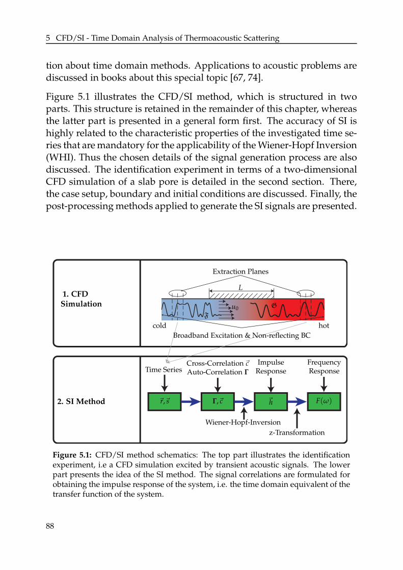
5 CFD/SI - Time Domain Analysis of Thermoacoustic Scattering
tion about time domain methods. Applications to acoustic problems arediscussed in books about this special topic [67, 74].
Figure 5.1 illustrates the CFD/SI method, which is structured in twoparts. This structure is retained in the remainder of this chapter, whereasthe latter part is presented in a general form first. The accuracy of SI ishighly related to the characteristic properties of the investigated time se-ries that are mandatory for the applicability of the Wiener-Hopf Inversion(WHI). Thus the chosen details of the signal generation process are alsodiscussed. The identification experiment in terms of a two-dimensionalCFD simulation of a slab pore is detailed in the second section. There,the case setup, boundary and initial conditions are discussed. Finally, thepost-processing methods applied to generate the SI signals are presented.
0.2
1. CFDSimulation
2. SI Method
Extraction Planes
cold
Broadband Excitation & Non-reflecting BC
hot
G
F
u0
L
Time SeriesCross-Correlation~cAuto-Correlation Γ
ImpulseResponse
FrequencyResponse
z-Transformation
Wiener-Hopf-Inversion
~r,~s F(ω)Γ,~c ~h
Figure 5.1: CFD/SI method schematics: The top part illustrates the identificationexperiment, i.e a CFD simulation excited by transient acoustic signals. The lowerpart presents the idea of the SI method. The signal correlations are formulated forobtaining the impulse response of the system, i.e. the time domain equivalent of thetransfer function of the system.
88
5.1 System Identification
5.1 System Identification
In general, if the suppression of unstable eigenmodes is possible insidean identification experiment – in this case the CFD simulation of a TAstack – predicting its scattering behavior for a single frequency is straight-forward. The single frequency based technique described in Section 4.6directly yields one set of scattering matrix coefficients. In mean flowaffected CFD simulations, pressure and velocity conditions are usuallyfixed at different locations [142]. The two-source location method is pre-ferred for such investigations. Forcing a sinusoidal excitation at the up-stream velocity BC for generating one state and driving the pressure atthe downstream end to yield a second state allows a direct applicationof Equation (4.68). The computational cost for this process scales linearlywith the number of frequencies considered. Thus SI methods are used torecover the complete frequency response from one single simulation runin the time domain.
The CFD/SI method is restricted to linear time-invariant systems (LTI)[155]. A system is linear if the principle of superposition [107] can beapplied. The time invariance of a system states that the output of thesystem does not depend on the actual time [155].
More background information of the CFD/SI method is presented in de-tail in various Ph. D. thesis (e.g. [75, 192]). Only the main equations ofthe process sketched in the second part of Figure 5.1 are given in the fol-lowing. As stated in Section 3.2.4.1, the chosen scattering matrix notationis causal, which further simplifies the theory. In the first step of the SIprocess denoted by WHI, the time series obtained are stored in terms ofsignals~s and responses~r. In a second step, the auto-correlation matrix Γ
of the input signals and the cross-correlation vector ~c of the in- and out-put signals [74] are generated. Solving the Wiener-Hopf equation [208]
~h = Γ−1~c. (5.1)
yields the unit impulse response (UIR) vector~h of the approximated sys-tem. This UIR, the output of the system to a Dirac delta impulse, is thetime domain equivalent of the frequency response F(ω), which is ob-
tained by a z-transformation of~h [110, 116].
89
5 CFD/SI - Time Domain Analysis of Thermoacoustic Scattering
As the WHI equation is the quintessence of the SI method, its functional-ity is considered in more detail. It approximates the discrete problem asan output error black-box model [155], i.e.
ri =∞
∑k=0
hksi−k + ei. (5.2)
The first term denotes the response of the system without noise. Thesecond accounts for noise e imposed on the response signals. Neglecting
contributions of large time scales, the length of~h reduces and it becomesa finite impulse response (FIR).
The size of ~h is determined by two time lags τ. The discretized timestep has to be considerably smaller than the minimum expected time lagτmin. Usually, the time step applied in CFD simulations is controlled byeven smaller time scales, for example turbulence, CFL-number, etc. Forresolving this mismatch between these time scales, a reduction factor mis introduced, which accounts for the discrepancy of expected minimumtime lag and temporal resolution. The maximum time lag consideredlimits the length of the FIR. Using this resolution, the length K = mL ofa discretized FIR has to be chosen such that at least the largest expectedtime lag τmax can be captured by the FIR. The Wiener Filter has noisesuppressing characteristics [63] that are reduced with increasing t(K) ≫τmax. Thus, the filter length mL has to be determined iteratively to findan optimum balance between noise suppression and system modeling.
The idea of the WHI method is to find a linear least squares optimum ofthe error-affected black-box model by minimizing the cost function
V(~h) =N
∑i=L+1
e2i (5.3)
in terms of
minh
(
V(~h))
. (5.4)
For given ~s and~r, this problem has an analytical solution. Finding theroot of its first derivative with respect to hj yields the optimum UIR.Substituting Equation (5.2) into the right hand side directly yields the
90
5.1 System Identification
Wiener-Hopf Equation (5.1). There, the sums of signals and responsesare formulated in terms of cross-correlation vector~c
ci =1
N − mL + 1
N
∑k=L
r(k)s(k − mi + 1) (5.5)
with i = 1, 2, 3, ..., K
and auto-correlation matrix Γ
Γij =1
N − mL + 1
N
∑k=L
s(k − mi + 1)s(k − mj + 1) (5.6)
with i, j = 1, 2, 3, ..., K.
This equation, also denoted as Wiener Filter [67], yields the linear leastsquares estimator for the FIR.
The solution method applied to Equation (5.1) has a certain impact on theresulting FIR. If iterative solvers are used, the noise content in the filter ispartially suppressed by tolerating a certain residual value. This is equiv-alent to introducing a regression factor in this equation that accounts fora certain amount of errors. Thus a LSQR method [133] with a standardresidual of 10−11 is applied to solve Equation (5.1).
The LSQR method is designed for sparse matrices. Applying this tech-nique in the matrix inversion in Equation (5.1) makes a good decorrela-tion of the input signals~s a crucial requirement to the signals. Here, thediagonal structure of the auto-correlation matrix is maximized by opti-mization of the reduction factor m. Considering each m-th signal datapoint only in Equation (5.6) causes a reduction in the off-diagonal contri-butions.
A second way of obtaining an optimized auto-correlation matrix relies ona good choice of the excitation signals. Thus, in MIMO systems, a gooddecorrelation of the input signals and a fast decorrelation of the signalitself accelerate the solution procedure. The auto-correlation matrix of awhite noise signal reduces to the unity matrix I [116]. For a finite signallength N the frequency content is not constant. The identification of thecorresponding transfer functions values might yield insufficient results.
An optimum signal is a trade off between this requirement and physicalconsiderations. On the one hand, a high signal to noise ratio ensures a
91
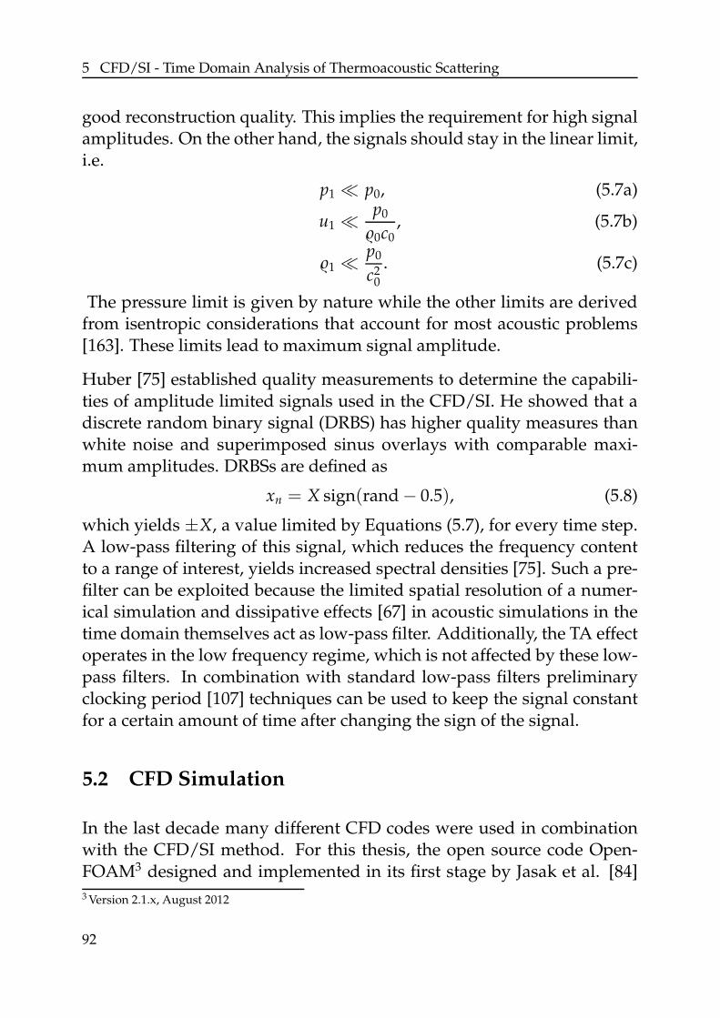
5 CFD/SI - Time Domain Analysis of Thermoacoustic Scattering
good reconstruction quality. This implies the requirement for high signalamplitudes. On the other hand, the signals should stay in the linear limit,i.e.
p1 ≪ p0, (5.7a)
u1 ≪p0
0c0, (5.7b)
1 ≪p0
c20
. (5.7c)
The pressure limit is given by nature while the other limits are derivedfrom isentropic considerations that account for most acoustic problems[163]. These limits lead to maximum signal amplitude.
Huber [75] established quality measurements to determine the capabili-ties of amplitude limited signals used in the CFD/SI. He showed that adiscrete random binary signal (DRBS) has higher quality measures thanwhite noise and superimposed sinus overlays with comparable maxi-mum amplitudes. DRBSs are defined as
xn = X sign(rand − 0.5), (5.8)
which yields ±X, a value limited by Equations (5.7), for every time step.A low-pass filtering of this signal, which reduces the frequency contentto a range of interest, yields increased spectral densities [75]. Such a pre-filter can be exploited because the limited spatial resolution of a numer-ical simulation and dissipative effects [67] in acoustic simulations in thetime domain themselves act as low-pass filter. Additionally, the TA effectoperates in the low frequency regime, which is not affected by these low-pass filters. In combination with standard low-pass filters preliminaryclocking period [107] techniques can be used to keep the signal constantfor a certain amount of time after changing the sign of the signal.
5.2 CFD Simulation
In the last decade many different CFD codes were used in combinationwith the CFD/SI method. For this thesis, the open source code Open-FOAM3 designed and implemented in its first stage by Jasak et al. [84]
3 Version 2.1.x, August 2012
92
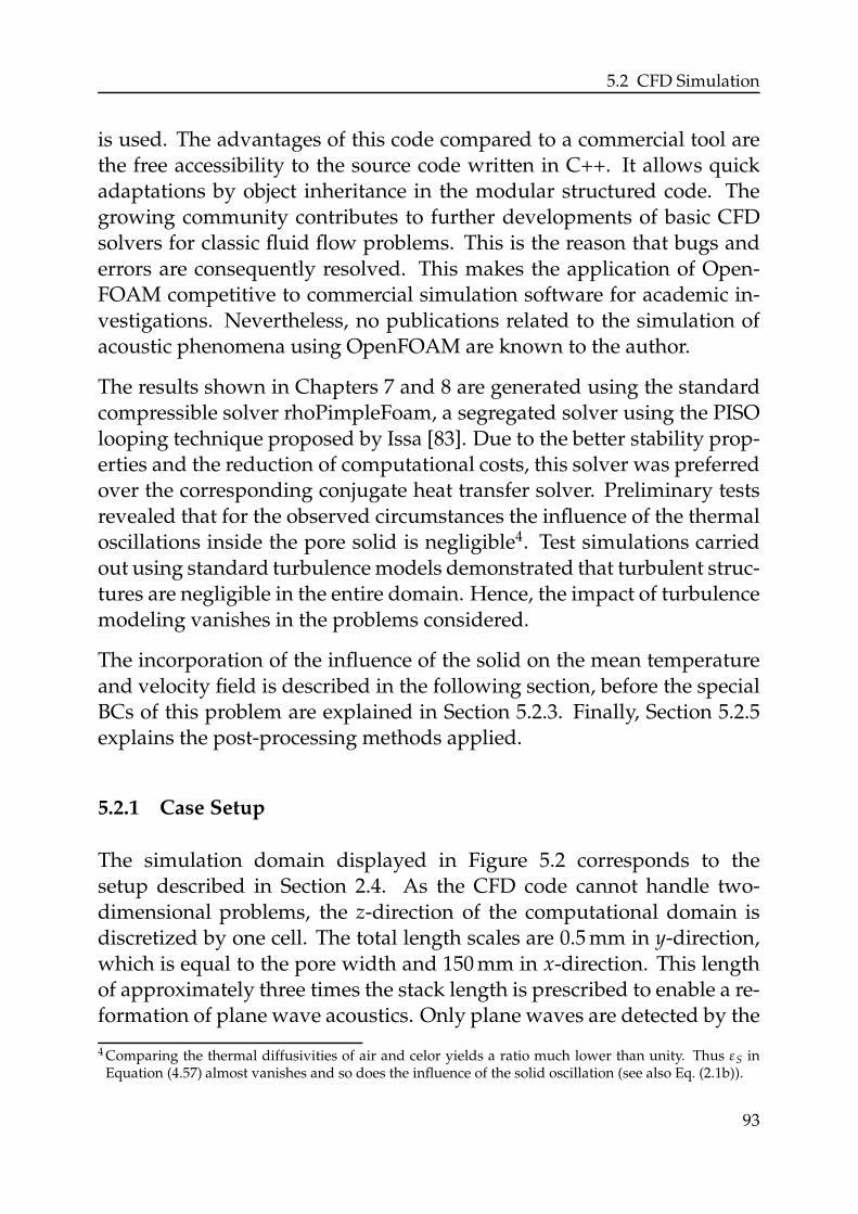
5.2 CFD Simulation
is used. The advantages of this code compared to a commercial tool arethe free accessibility to the source code written in C++. It allows quickadaptations by object inheritance in the modular structured code. Thegrowing community contributes to further developments of basic CFDsolvers for classic fluid flow problems. This is the reason that bugs anderrors are consequently resolved. This makes the application of Open-FOAM competitive to commercial simulation software for academic in-vestigations. Nevertheless, no publications related to the simulation ofacoustic phenomena using OpenFOAM are known to the author.
The results shown in Chapters 7 and 8 are generated using the standardcompressible solver rhoPimpleFoam, a segregated solver using the PISOlooping technique proposed by Issa [83]. Due to the better stability prop-erties and the reduction of computational costs, this solver was preferredover the corresponding conjugate heat transfer solver. Preliminary testsrevealed that for the observed circumstances the influence of the thermaloscillations inside the pore solid is negligible4. Test simulations carriedout using standard turbulence models demonstrated that turbulent struc-tures are negligible in the entire domain. Hence, the impact of turbulencemodeling vanishes in the problems considered.
The incorporation of the influence of the solid on the mean temperatureand velocity field is described in the following section, before the specialBCs of this problem are explained in Section 5.2.3. Finally, Section 5.2.5explains the post-processing methods applied.
5.2.1 Case Setup
The simulation domain displayed in Figure 5.2 corresponds to thesetup described in Section 2.4. As the CFD code cannot handle two-dimensional problems, the z-direction of the computational domain isdiscretized by one cell. The total length scales are 0.5 mm in y-direction,which is equal to the pore width and 150 mm in x-direction. This lengthof approximately three times the stack length is prescribed to enable a re-formation of plane wave acoustics. Only plane waves are detected by the
4 Comparing the thermal diffusivities of air and celor yields a ratio much lower than unity. Thus εS inEquation (4.57) almost vanishes and so does the influence of the solid oscillation (see also Eq. (2.1b)).
93
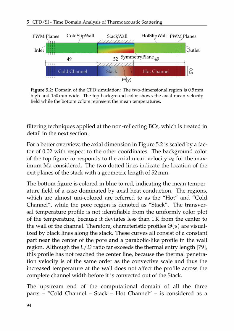
5 CFD/SI - Time Domain Analysis of Thermoacoustic Scattering
OutletInlet
HotSlipWallColdSlipWall StackWall PWM PlanesPWM Planes
SymmetryPlane
Hot ChannelCold Channel Stack
Θ(y)
495249
0.5
Figure 5.2: Domain of the CFD simulation: The two-dimensional region is 0.5 mmhigh and 150 mm wide. The top background color shows the axial mean velocityfield while the bottom colors represent the mean temperatures.
filtering techniques applied at the non-reflecting BCs, which is treated indetail in the next section.
For a better overview, the axial dimension in Figure 5.2 is scaled by a fac-tor of 0.02 with respect to the other coordinates. The background colorof the top figure corresponds to the axial mean velocity u0 for the max-imum Ma considered. The two dotted lines indicate the location of theexit planes of the stack with a geometric length of 52 mm.
The bottom figure is colored in blue to red, indicating the mean temper-ature field of a case dominated by axial heat conduction. The regions,which are almost uni-colored are referred to as the “Hot” and “ColdChannel”, while the pore region is denoted as “Stack”. The transver-sal temperature profile is not identifiable from the uniformly color plotof the temperature, because it deviates less than 1 K from the center tothe wall of the channel. Therefore, characteristic profiles Θ(y) are visual-ized by black lines along the stack. These curves all consist of a constantpart near the center of the pore and a parabolic-like profile in the wallregion. Although the L/D ratio far exceeds the thermal entry length [79],this profile has not reached the center line, because the thermal penetra-tion velocity is of the same order as the convective scale and thus theincreased temperature at the wall does not affect the profile across thecomplete channel width before it is convected out of the Stack.
The upstream end of the computational domain of all the threeparts – “Cold Channel – Stack – Hot Channel” – is considered as a
94
5.2 CFD Simulation
“SymmetryPlane”, which is physical for laminar and turbulent simula-tions using unsteady Reynolds averaged Navier-Stokes (URANS) equa-tions. Due to the different nature of both Channels and the intermediateStack, the opposite boundary is split into three parts: the “StackWall” isa no-slip wall with fixed temperature values, while the “ColdSlipWall”and “HotSlipWall” are adiabatic no-slip walls. The “Inlet” and “Outlet”are especially designed boundaries, see Section 5.2.3.
The Stack is resolved into cells that have a constant cell width ∆x =10−4m. The cell height decays linearly in the positive y-direction. Thisresults in a mesh size of 520 × 20 cells for this region. Using this cell sizeand an acoustic CFL-number less than unity (Eq. (2.3)) yields a simula-tion time step of ∆t = 1.25 × 10⁻⁷ s. As the inflow and outflow condi-tions of the stack are multidimensional problems, a certain part of theChannels has to be resolved sufficiently (Figure 5.3) to capture the flowfield in the vicinity of the inlet stagnation point. Furthermore, the flowfield downstream of the stack has to be resolved up to the point wheretransversal differences in the flow field are negligible. Due to convection,the latter effect, which is of the order of [104]
Ld
R≈ 0.1 Re, (5.9)
extends over a wider region than the first. For the maximum velocityconsidered here this approximation leads to
Ld / 4 × 10⁻³ m. (5.10)
16 H 12 H
0.5
H
intermediatecoarse fine
Figure 5.3: Zone of mesh refinement: the mesh is symmetric with respect to thecenter plane of the stack.
95
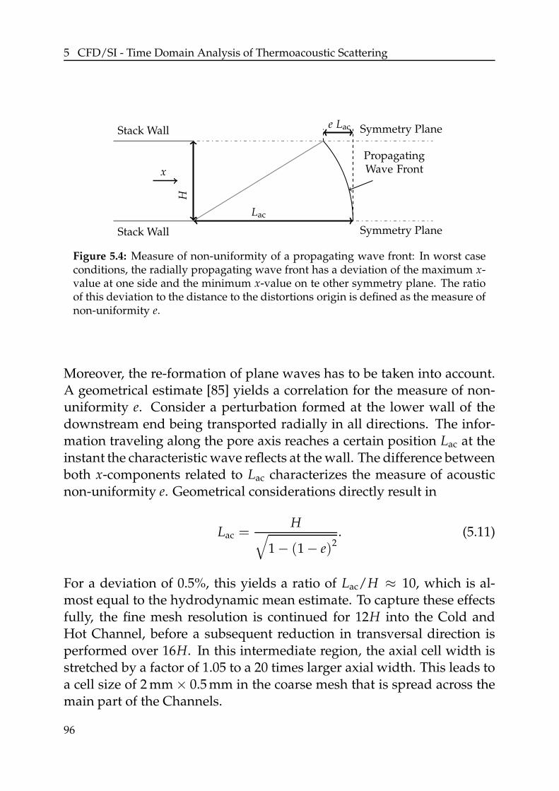
5 CFD/SI - Time Domain Analysis of Thermoacoustic Scattering
Hx
Symmetry Plane
Symmetry Plane
Stack Wall
Stack Wall
Lac
e Lac
PropagatingWave Front
Figure 5.4: Measure of non-uniformity of a propagating wave front: In worst caseconditions, the radially propagating wave front has a deviation of the maximum x-value at one side and the minimum x-value on te other symmetry plane. The ratioof this deviation to the distance to the distortions origin is defined as the measure ofnon-uniformity e.
Moreover, the re-formation of plane waves has to be taken into account.A geometrical estimate [85] yields a correlation for the measure of non-uniformity e. Consider a perturbation formed at the lower wall of thedownstream end being transported radially in all directions. The infor-mation traveling along the pore axis reaches a certain position Lac at theinstant the characteristic wave reflects at the wall. The difference betweenboth x-components related to Lac characterizes the measure of acousticnon-uniformity e. Geometrical considerations directly result in
Lac =H
√
1 − (1 − e)2. (5.11)
For a deviation of 0.5%, this yields a ratio of Lac/H ≈ 10, which is al-most equal to the hydrodynamic mean estimate. To capture these effectsfully, the fine mesh resolution is continued for 12H into the Cold andHot Channel, before a subsequent reduction in transversal direction isperformed over 16H. In this intermediate region, the axial cell width isstretched by a factor of 1.05 to a 20 times larger axial width. This leads toa cell size of 2 mm × 0.5 mm in the coarse mesh that is spread across themain part of the Channels.
96
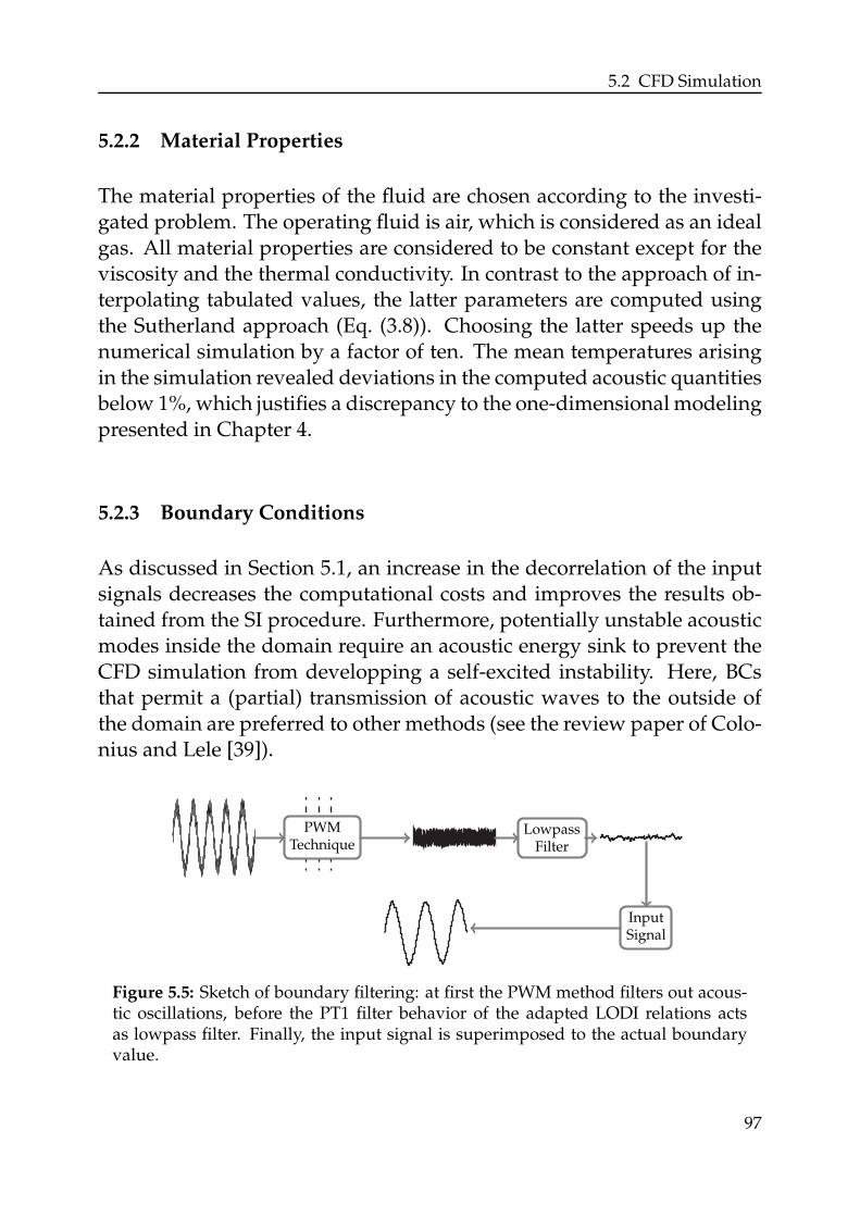
5.2 CFD Simulation
5.2.2 Material Properties
The material properties of the fluid are chosen according to the investi-gated problem. The operating fluid is air, which is considered as an idealgas. All material properties are considered to be constant except for theviscosity and the thermal conductivity. In contrast to the approach of in-terpolating tabulated values, the latter parameters are computed usingthe Sutherland approach (Eq. (3.8)). Choosing the latter speeds up thenumerical simulation by a factor of ten. The mean temperatures arisingin the simulation revealed deviations in the computed acoustic quantitiesbelow 1%, which justifies a discrepancy to the one-dimensional modelingpresented in Chapter 4.
5.2.3 Boundary Conditions
As discussed in Section 5.1, an increase in the decorrelation of the inputsignals decreases the computational costs and improves the results ob-tained from the SI procedure. Furthermore, potentially unstable acousticmodes inside the domain require an acoustic energy sink to prevent theCFD simulation from developping a self-excited instability. Here, BCsthat permit a (partial) transmission of acoustic waves to the outside ofthe domain are preferred to other methods (see the review paper of Colo-nius and Lele [39]).
PWMTechnique
LowpassFilter
InputSignal
Figure 5.5: Sketch of boundary filtering: at first the PWM method filters out acous-tic oscillations, before the PT1 filter behavior of the adapted LODI relations actsas lowpass filter. Finally, the input signal is superimposed to the actual boundaryvalue.
97
5 CFD/SI - Time Domain Analysis of Thermoacoustic Scattering
The signal treatment at these BCs is sketched in Figure 5.5. Kreiss[97] proposed the so-called “local associated one-dimensional inviscid”(LODI) relations. This set of equations is a simplified version of theone-dimensional linearized equations of motion discussed in Section 3.1.Thompson [195, 196] used these LODI relations as an estimate of thewaves entering and leaving the domain in the computation of BCs forinviscid flow problems. Based on his formulation Poinsot and Lele [142]derived a similar set for the application in compressible CFD simula-tions. These “Navier-Stokes based characteristic boundary conditions”(NSCBC), which suppress the reflections normal to the boundary, werefurther expanded by different authors [108, 213, 214] to additionally ap-ply for transversal directions and species transport.
Here, a less sophisticated version was implemented. As the objective ofthis study was to investigate laminar flow problems coupled with acous-tics, no problems that arise from combustion [141] or turbulence have tobe taken into account. The distances from the Stack end to the inlet andoutlet boundary is very large. In combination with the chosen symmetryconditions at the boundaries normal to the y-direction reduce possiblytransported vorticity waves to a minimum. Moreover, the interaction be-tween acoustic and vorticity waves is restricted to high Mach numbers.Still, small perturbations may approach the Outlet. Close investigationsof the Hot Channel revealed negligible non-acoustic oscillations. Hence,the relevant fluctuations that approach the boundaries are assumed topropagate in isentropic conditions. This implies that only the reflectivityof the acoustic quantities of velocity and pressure have to be considered.General considerations lead to the conclusion that a well-posed set ofBCs for a subsonic compressible flow problem consists of a pressure BCat the outlet and Dirichlet conditions for the velocity at the inlet of the do-main [142]. To ensure this well-posedness, Rudy and Strickwerda [172]expanded the LODI relations by a relaxation term, such that the reflectiv-ity of these BCs is not fully non-reflective [176, 181], especially in the lowfrequency range.
Polifke et al. [152] suggested an additional filter technique that improvesthe lowpass characteristic of the existing BCs based on filtering acousticwaves [148]. Kopitz et al. [94] developed such a characteristics basedfilter to extract the acoustic characteristic wave amplitudes at certain
98
5.2 CFD Simulation
monitor planes near the non-reflective boundary. An instantaneous areaaveraging yields the acoustic quantities by the application of a simplemoving average technique in time [91]. These data are shifted by thecharacteristic acoustic time scale to the instant at which they arise at theboundary. Averaging over the monitor planes leads to a good estimateof the boundary normal acoustic quantity. Subtracting this value fromits instant field value reduces the quantity, which has to be relaxed by itsacoustic component. This process is referred to as “plane wave masking”and is explained in detail by Polifke et al. [152]. The combination of thesetwo techniques was first applied by Kaess et al. [86] to form an acousticimpedance BC, which he demonstrated to be very accurate [88].
The last two steps sketched in Figure 5.5 describe the signal generation atthe boundaries. An additional forcing term in the BCs facilitates the gen-eration of characteristic wave amplitudes [88] traveling into the domain.Here, this method is used to insert the time line of the input signals atthe corresponding BCs. Preliminary tests revealed a good agreement ofdesired and generated input signals for the chosen geometry.
5.2.4 Initial Conditions
The mean field quantities provide the steady state background informa-tion for the acoustic propagation mechanisms. As temperature and ve-locity directly couple with the TATEs (Eq. (4.36)), this information has tobe adapted for all observed cases, i.e. changes in terms of Pe and Ma. Inparticular the non-constant temperature at the “StackWall” boundary hasto be determined in a preliminary process to account for the mean heatconduction in the non-resolved solid domain. Starting with an approx-imate solution obtained from Equation (4.33), a conjugate heat transferproblem was solved by an iterative application of a finite element tech-nique5 on a computational domain containing the full fluid and solid partof one observed regenerator pore and its axial vicinity. The reference val-ues at the cold inlet are fixed. For comparability, an averaged fluid Outlettemperature is sought. This condition is verified by adapting the temper-ature value at the hot end of the solid regenerator wall. It is found usinga gradient-based method, allowing for a deviation of less than 1 K from5 Conjugate Heat Transfer Toolbox, Comsol 6.2 [40].
99
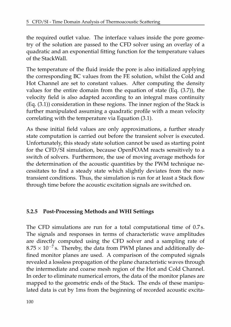
5 CFD/SI - Time Domain Analysis of Thermoacoustic Scattering
the required outlet value. The interface values inside the pore geome-try of the solution are passed to the CFD solver using an overlay of aquadratic and an exponential fitting function for the temperature valuesof the StackWall.
The temperature of the fluid inside the pore is also initialized applyingthe corresponding BC values from the FE solution, whilst the Cold andHot Channel are set to constant values. After computing the densityvalues for the entire domain from the equation of state (Eq. (3.7)), thevelocity field is also adapted according to an integral mass continuity(Eq. (3.1)) consideration in these regions. The inner region of the Stack isfurther manipulated assuming a quadratic profile with a mean velocitycorrelating with the temperature via Equation (3.1).
As these initial field values are only approximations, a further steadystate computation is carried out before the transient solver is executed.Unfortunately, this steady state solution cannot be used as starting pointfor the CFD/SI simulation, because OpenFOAM reacts sensitively to aswitch of solvers. Furthermore, the use of moving average methods forthe determination of the acoustic quantities by the PWM technique ne-cessitates to find a steady state which slightly deviates from the non-transient conditions. Thus, the simulation is run for at least a Stack flowthrough time before the acoustic excitation signals are switched on.
5.2.5 Post-Processing Methods and WHI Settings
The CFD simulations are run for a total computational time of 0.7 s.The signals and responses in terms of characteristic wave amplitudesare directly computed using the CFD solver and a sampling rate of8.75 × 10−7 s. Thereby, the data from PWM planes and additionally de-fined monitor planes are used. A comparison of the computed signalsrevealed a lossless propagation of the plane characteristic waves throughthe intermediate and coarse mesh region of the Hot and Cold Channel.In order to eliminate numerical errors, the data of the monitor planes aremapped to the geometric ends of the Stack. The ends of these manipu-lated data is cut by 1ms from the beginning of recorded acoustic excita-
100

5.2 CFD Simulation
tion before they are passed to the WHI tool to improve the independenceof transients.
The preliminary data manipulation results in signal lengths of N ≈80000. All signals are pre-filtered using a low-pass filter with a cut offrequency of 100 Hz. A close investigation of the WHI filter length andthe reduction factor yielded optimum parameters of L = 100 and m = 25,which are applied to all simulation cases considered.
101

5 CFD/SI - Time Domain Analysis of Thermoacoustic Scattering
102
6 Experimental Determination of Thermoa-coustic Effects
The credibility of numerically acquired results is always dependent uponmodeling assumptions. Different approaches of modeling a complexproblem lead to increased reliability, but only experimental data supporttheir validity. As stated in Section 2.2, for the investigated TA problem,no data are available in literature (to the author’s knowledge).
Experimentally determining the acoustic fields under non-isentropic con-ditions is challenging. The characteristic wave amplitudes F and G can-not be measured by a direct method. Acoustic velocity fluctuations u1 arecomputed from optical methods using LDA [20] or PIV [3, 23] methods.The coupling of the acoustic pressure p1 to temperature T1 and density1 fluctuations by the linearized equation of state (4.36a) requires simul-taneous investigation of these two quantities. p1 cannot be determineddirectly in spatially resolved form. If possible, T1 and 1 have to be cap-tured for finding spatially resolved relations in terms of u1, p1. In addi-tion, providing optical access to the region of interest is often challenging.Furthermore, generating simultaneous measurement data for differentfields is cost-intensive and time demanding. Thus, this approach is outof the scope of this study.
Many acoustic investigation methods rely on approximating the acousticfield with analytical formulations which are fitted to local probe values.Investigating directed velocity fluctuations u1 is straightforward by usingconstant temperature anemometry [76]. Dynamic pressure probes usepiezoelectric sensor technology or classic capacitive microphones. Here,the latter are chosen for the construction of the cross-sectionally averagedacoustic state vectors providing reference data for the scattering behavior.
For the purpose of generating these data by applying the multi micro-phone method (MMM), an experimental apparatus is designed and setup. Its modular design further facilitates operating the test rig in a TA
103
6 Experimental Determination of Thermoacoustic Effects
standing wave engine configuration. The acoustic power produced in-side the regenerator is not absorbed by any load. The driving effectsinside the system are solely balanced by dissipative effects. For the pur-pose of separating the device from a heat pumping apparatus, it is stillreferred to as an “engine”. The self-excited oscillations occurring therebyprovide a qualitative demonstration of TA energy conversion using theregenerators. Moreover, a validation of the scattering matrix entries forone operating frequency by the time-dependent pressure data is possible.
The first two parts of this chapter discuss the theoretical background ofthe measurement technique applied and provide the link to theoreticalinformation that can be drawn from the different measurements. Thechapter concludes with a presentation of the design of the experimentalapparatus in Section 6.3.
6.1 Multi Microphone Method
The MMM is a standard technique in duct-acoustics to determine theacoustic scattering behavior of acoustic multi-ports. In general, the ap-plication of the experimental MMM results in complex-valued transferor scattering matrices. The idea is to determine the characteristic waveamplitudes at the ports of the investigated acoustic element by findingthe optimum of an overdetermined system of equations that is estimatedto fit the spatial profile of the acoustic pressure outside the element. Thistechnique is a derivate of the two-source location method in referenceto Section 4.6. The idea is to establish two independent acoustic states,which provide the information yielding the transfer matrix componentsof the considered acoustic two-port. In contrast to the application of thistechnique in the one-dimensional tool presented in Section 4.6, the up-and downstream values of p1 and u1 at the reference planes of the mod-eled element are not provided directly. They have to be found by re-constructing them from the measured data at the probing locations. Thereconstruction is based on the mean temperature and velocity field in themeasurement ducts, which has to be modeled.
104

6.1 Multi Microphone Method
6.1.1 Two Microphone Method and its Development
In 1979, To and Doige [198, 199] invented the two-load method, whichwas the first method to obtain transfer matrices experimentally. Theydemonstrated its capability for six geometries consisting of pipes, ex-pansion and contraction chambers. The experimental setup was drivenupstream of the measurement positions. Two independent states werecreated by applying a variable load at the opposite end of the measure-ment setup, which manipulated the acoustic impedance at the down-stream end of their test rig. The pressure data were acquired using onemicrophone located at two varying positions inside each measurementchannel.
In collaboration with Lung, Doige [109] further developed this methodby applying the four-microphone two-load method. This reduced theminimum number of necessary measurements by a factor of two. Theone-source two-load method, which theoretically always leads to inde-pendence of both states, reveals problems for certain frequencies becausethe two loads are not sufficiently different from each other for all frequen-cies observed.
Munjal and Doige [123] overcame this challenge by introducing a sec-ond acoustic source on the opposite side of the experiment. Based onthis method, various geometries and configurations were investigated[126, 127, 134, 147]. Abom and Boden [4, 27] investigated the impact ofmeasurement errors and derived limit spacings of the pressure sensors.Polifke and Paschereit [134, 147] proposed to increase the number of mi-crophones to reduce the error content of the analytically described fields.At the Lehrstuhl fur Thermodynamik of TU Munchen this idea was im-plemented by Fischer [56] to investigate the acoustic transfer matrix of aswirl burner. The same method was also used by the group of Paschereitand Schueller to validate the analytical modeling of the acoustic transferof different turbulent premixed burner configurations [135, 178, 179].
Minimizing the data error by applying a least squares fit method tothe now overdetermined system improved the confidence of resultsby reducing the impact of measurement error of each pressure probe.Neunertf [126, 127] addressed the reconstruction error for thermally af-
105

6 Experimental Determination of Thermoacoustic Effects
fected measurements. He transformed the functional spatial expressionof the estimated pressure profile to a chain of acoustic two-ports describ-ing the wave characteristics between the measurement positions. By thismethod, he expanded the applicability of the MMM to arbitrary mea-surement regions with given acoustic transmission behavior. The lattermethodology is applied to the current configuration, which is presentedin the next section.
6.1.2 Multi Microphone Method in Non-Isentropic Conditions
The measurement setup is sketched in Figure 6.1. The goal of the MMMis to determine the scattering matrix for the acoustic black-box elementbased on the approximated spatial profile of the acoustic pressure p1.Here, the investigated black-box two-port represents the thermoacousticcore, i.e. the combination of the TA stack and its adjacent heat exchang-ers. As stated before, generating two independent acoustic states yields alinear system of equations in terms of Equation (4.68) or its equivalent inpu-notation. The reference locations xu,d,ref are defined by the upstreamand downstream location of the interface between the acoustic two-portand the test rig. In many configurations, a direct access to the acous-tic quantities at these locations is not realizable. Furthermore, the re-
xu,1 xu,2 xu,i xu,N xd,1 xd,2 xd,j xd,M
u0
TA core
xu,re f
Sp
eak
er
Sp
eak
er
xd,re f
FdFu
GdGu
HX
Stack Downstream DuctUpstream Duct
Figure 6.1: Sketch of the MMM applied to the present configuration. The investi-gated TA core is connected to an ambient duct at the upstream side and a hot ductwith varying mean temperature at the downstream port. If mean flow is applied itflows from the ambient “Upstream Duct” to the heated “Downstream Duct”. Bothducts are supplied with a speaker and various microphone probes in order to gen-erate and determine two acoustic states at the reference positions xu,d,ref.
106
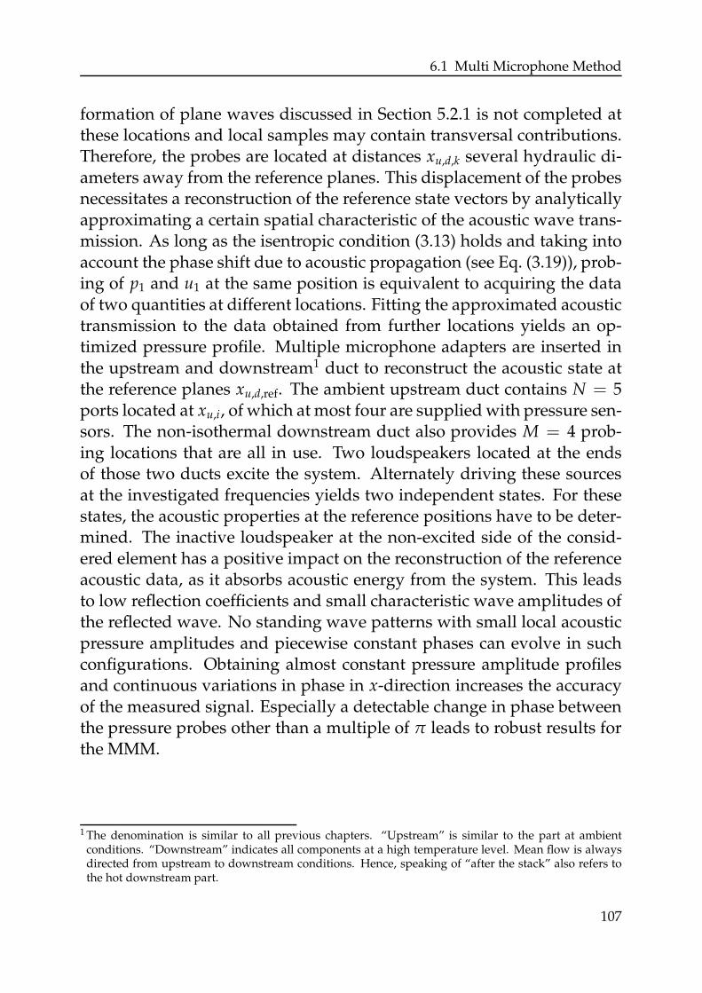
6.1 Multi Microphone Method
formation of plane waves discussed in Section 5.2.1 is not completed atthese locations and local samples may contain transversal contributions.Therefore, the probes are located at distances xu,d,k several hydraulic di-ameters away from the reference planes. This displacement of the probesnecessitates a reconstruction of the reference state vectors by analyticallyapproximating a certain spatial characteristic of the acoustic wave trans-mission. As long as the isentropic condition (3.13) holds and taking intoaccount the phase shift due to acoustic propagation (see Eq. (3.19)), prob-ing of p1 and u1 at the same position is equivalent to acquiring the dataof two quantities at different locations. Fitting the approximated acoustictransmission to the data obtained from further locations yields an op-timized pressure profile. Multiple microphone adapters are inserted inthe upstream and downstream1 duct to reconstruct the acoustic state atthe reference planes xu,d,ref. The ambient upstream duct contains N = 5ports located at xu,i, of which at most four are supplied with pressure sen-sors. The non-isothermal downstream duct also provides M = 4 prob-ing locations that are all in use. Two loudspeakers located at the endsof those two ducts excite the system. Alternately driving these sourcesat the investigated frequencies yields two independent states. For thesestates, the acoustic properties at the reference positions have to be deter-mined. The inactive loudspeaker at the non-excited side of the consid-ered element has a positive impact on the reconstruction of the referenceacoustic data, as it absorbs acoustic energy from the system. This leadsto low reflection coefficients and small characteristic wave amplitudes ofthe reflected wave. No standing wave patterns with small local acousticpressure amplitudes and piecewise constant phases can evolve in suchconfigurations. Obtaining almost constant pressure amplitude profilesand continuous variations in phase in x-direction increases the accuracyof the measured signal. Especially a detectable change in phase betweenthe pressure probes other than a multiple of π leads to robust results forthe MMM.
1 The denomination is similar to all previous chapters. “Upstream” is similar to the part at ambientconditions. “Downstream” indicates all components at a high temperature level. Mean flow is alwaysdirected from upstream to downstream conditions. Hence, speaking of “after the stack” also refers tothe hot downstream part.
107
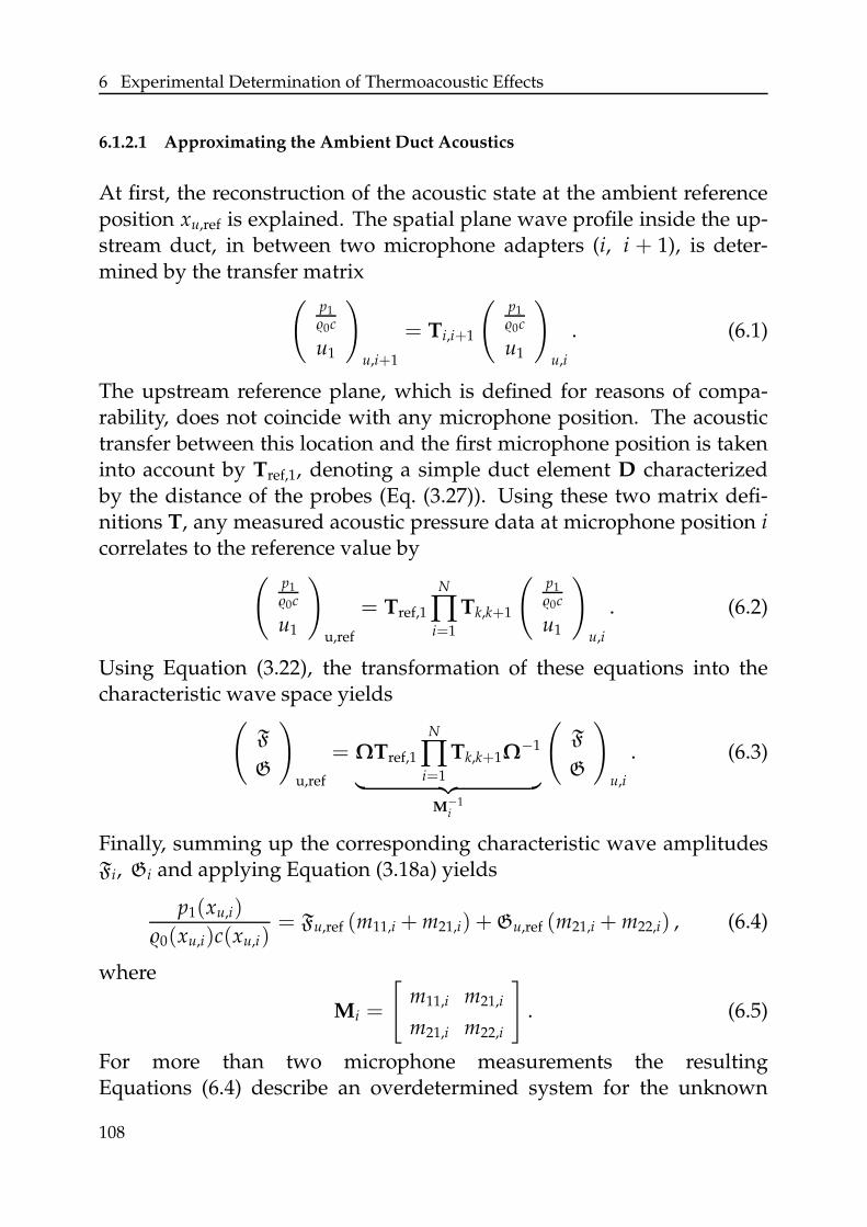
6 Experimental Determination of Thermoacoustic Effects
6.1.2.1 Approximating the Ambient Duct Acoustics
At first, the reconstruction of the acoustic state at the ambient referenceposition xu,ref is explained. The spatial plane wave profile inside the up-stream duct, in between two microphone adapters (i, i + 1), is deter-mined by the transfer matrix
(p1
0c
u1
)
u,i+1
= Ti,i+1
(p1
0c
u1
)
u,i
. (6.1)
The upstream reference plane, which is defined for reasons of compa-rability, does not coincide with any microphone position. The acoustictransfer between this location and the first microphone position is takeninto account by Tref,1, denoting a simple duct element D characterizedby the distance of the probes (Eq. (3.27)). Using these two matrix defi-nitions T, any measured acoustic pressure data at microphone position icorrelates to the reference value by
(p10c
u1
)
u,ref
= Tref,1
N
∏i=1
Tk,k+1
(p10c
u1
)
u,i
. (6.2)
Using Equation (3.22), the transformation of these equations into thecharacteristic wave space yields
(
F
G
)
u,ref
= ΩTref,1
N
∏i=1
Tk,k+1Ω−1
︸ ︷︷ ︸
M−1i
(
F
G
)
u,i
. (6.3)
Finally, summing up the corresponding characteristic wave amplitudesFi, Gi and applying Equation (3.18a) yields
p1(xu,i)
0(xu,i)c(xu,i)= Fu,ref (m11,i + m21,i) +Gu,ref (m21,i + m22,i) , (6.4)
where
Mi =
[
m11,i m21,i
m21,i m22,i
]
. (6.5)
For more than two microphone measurements the resultingEquations (6.4) describe an overdetermined system for the unknown
108
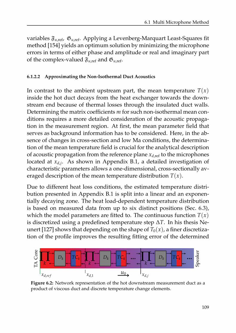
6.1 Multi Microphone Method
variables Fu,ref, Gu,ref. Applying a Levenberg-Marquart Least-Squares fitmethod [154] yields an optimum solution by minimizing the microphoneerrors in terms of either phase and amplitude or real and imaginary partof the complex-valued Fu,ref and Gu,ref.
6.1.2.2 Approximating the Non-Isothermal Duct Acoustics
In contrast to the ambient upstream part, the mean temperature T(x)inside the hot duct decays from the heat exchanger towards the down-stream end because of thermal losses through the insulated duct walls.Determining the matrix coefficients m for such non-isothermal mean con-ditions requires a more detailed consideration of the acoustic propaga-tion in the measurement region. At first, the mean parameter field thatserves as background information has to be considered. Here, in the ab-sence of changes in cross-section and low Ma conditions, the determina-tion of the mean temperature field is crucial for the analytical descriptionof acoustic propagation from the reference plane xd,ref to the microphoneslocated at xd,j. As shown in Appendix B.1, a detailed investigation ofcharacteristic parameters allows a one-dimensional, cross-sectionally av-eraged description of the mean temperature distribution T(x).
Due to different heat loss conditions, the estimated temperature distri-bution presented in Appendix B.1 is split into a linear and an exponen-tially decaying zone. The heat load-dependent temperature distributionis based on measured data from up to six distinct positions (Sec. 6.3),which the model parameters are fitted to. The continuous function T(x)is discretized using a predefined temperature step ∆T. In his thesis Ne-unert [127] shows that depending on the shape of T0(x), a finer discretiza-tion of the profile improves the resulting fitting error of the determined
... ...
xd,re f xd,1 xd,j
TCkTCkTCk DkDkDk ΠΠΠkkk
TA
Co
re
Sp
eak
er
u0
Figure 6.2: Network representation of the hot downstream measurement duct as aproduct of viscous duct and discrete temperature change elements.
109
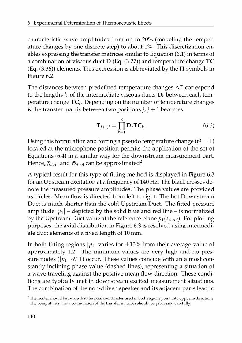
6 Experimental Determination of Thermoacoustic Effects
characteristic wave amplitudes from up to 20% (modeling the temper-ature changes by one discrete step) to about 1%. This discretization en-ables expressing the transfer matrices similar to Equation (6.1) in terms ofa combination of viscous duct D (Eq. (3.27)) and temperature change TC
(Eq. (3.36)) elements. This expression is abbreviated by the Π-symbols inFigure 6.2.
The distances between predefined temperature changes ∆T correspondto the lengths lk of the intermediate viscous ducts Dk between each tem-perature change TCk. Depending on the number of temperature changesK the transfer matrix between two positions j, j + 1 becomes
Tj+1,j =K
∏k=1
DkTCk. (6.6)
Using this formulation and forcing a pseudo temperature change (Θ = 1)located at the microphone position permits the application of the set ofEquations (6.4) in a similar way for the downstream measurement part.Hence, Fd,ref and Gd,ref can be approximated2.
A typical result for this type of fitting method is displayed in Figure 6.3for an Upstream excitation at a frequency of 140 Hz. The black crosses de-note the measured pressure amplitudes. The phase values are providedas circles. Mean flow is directed from left to right. The hot DownstreamDuct is much shorter than the cold Upstream Duct. The fitted pressureamplitude |p1| – depicted by the solid blue and red line – is normalizedby the Upstream Duct value at the reference plane p1(xu,ref). For plottingpurposes, the axial distribution in Figure 6.3 is resolved using intermedi-ate duct elements of a fixed length of 10 mm.
In both fitting regions |p1| varies for ±15% from their average value ofapproximately 1.2. The minimum values are very high and no pres-sure nodes (|p1| ≪ 1) occur. These values coincide with an almost con-stantly inclining phase value (dashed lines), representing a situation ofa wave traveling against the positive mean flow direction. These condi-tions are typically met in downstream excited measurement situations.The combination of the non-driven speaker and its adjacent parts lead to
2 The reader should be aware that the axial coordinates used in both regions point into opposite directions.The computation and accumulation of the transfer matrices should be processed carefully.
110
6.1 Multi Microphone Method
0
0
1
0.5
1.5
-π2
-π
π2
πM
agn
itu
de|
p1
pn
orm|[−]
Ph
ase
Φ(p
1)[r
ad]
xdxu
1 0.8 0.6 0.4 0.2 0 0.2 0.4
Upstream Duct Downstream Duct
Position xuLu[−] Position xd
Ld[−]
u0
Figure 6.3: Typical pressure fit for the MMM at an excitation frequency of 140 Hzwith four microphones at each side of the investigated acoustic element. Crossesand solid lines denote the experimental and analytically approximated magnitudeof pressure p1. Phases of p1 are denoted by circles and dashed lines respectively.Blue lines indicate the Upstream Duct, red lines the hot Downstream Duct. Theblack dashed line indicates both reference planes.
a small reflection coefficient. This non-zero, frequency-dependent coef-ficient causes a reflected wave which slightly modulates the pressure inphase and magnitude.
Comparing the measured data to the fit, the phases match better than theamplitude values. This phenomenon is always found, if the fitting is car-ried out for the real and imaginary part of the set of Equations (6.4). Thelarger discrepancies in the magnitude values are observed for all mea-surement conditions. Using four microphones leads to a good reliabilityof the data fit for most investigated frequencies.
6.1.3 Reconstruction from TA Core Data
In Chapters 4 and 5, the acoustic transmission of the regenerator was con-sidered analytically and numerically without the adjacent heat exchang-ers. This is not possible in the experimental setup. The mean temperatureis maintained by the heat exchangers. Thus, a direct investigation of thescattering behavior of the TA stack is impossible. An indirect methodhas to be applied, in which the heat exchangers are reconstructed fromseparate measurement campaigns. The reconstruction is illustrated in
111
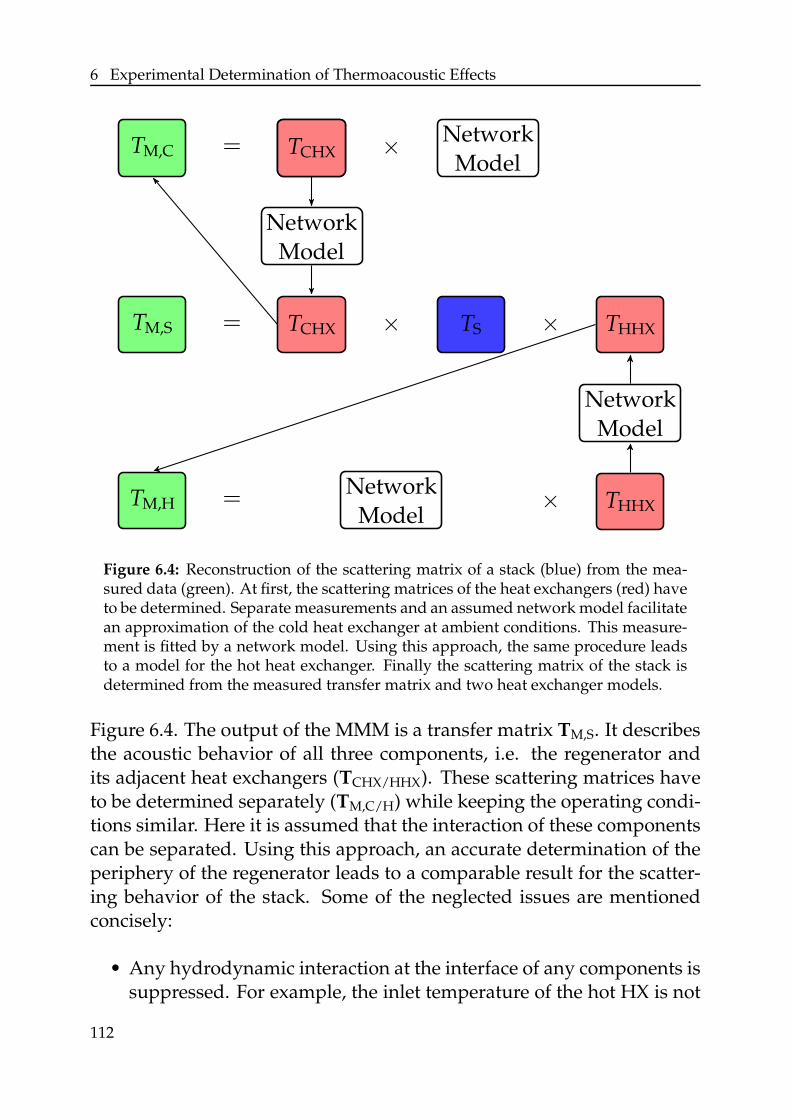
6 Experimental Determination of Thermoacoustic Effects
TM,S = TCHX × TS × THHX
Network
Model
Network
Model
TCHX=TM,C × Network
ModelTCHX
THHX×
Network
Model
TM,H =
Network
Model
Network
Model
Figure 6.4: Reconstruction of the scattering matrix of a stack (blue) from the mea-sured data (green). At first, the scattering matrices of the heat exchangers (red) haveto be determined. Separate measurements and an assumed network model facilitatean approximation of the cold heat exchanger at ambient conditions. This measure-ment is fitted by a network model. Using this approach, the same procedure leadsto a model for the hot heat exchanger. Finally the scattering matrix of the stack isdetermined from the measured transfer matrix and two heat exchanger models.
Figure 6.4. The output of the MMM is a transfer matrix TM,S. It describesthe acoustic behavior of all three components, i.e. the regenerator andits adjacent heat exchangers (TCHX/HHX). These scattering matrices haveto be determined separately (TM,C/H) while keeping the operating condi-tions similar. Here it is assumed that the interaction of these componentscan be separated. Using this approach, an accurate determination of theperiphery of the regenerator leads to a comparable result for the scatter-ing behavior of the stack. Some of the neglected issues are mentionedconcisely:
• Any hydrodynamic interaction at the interface of any components issuppressed. For example, the inlet temperature of the hot HX is not
112
6.1 Multi Microphone Method
changed by direct thermal contact with the stack. Further, the for-mation of streaming vortices might also be retarded by an adjacentcomponent.
• The increased blockage due to geometrical changes of the free sur-faces at the contact plane is assumed to have no effect. Imagine astack of plates at perfect contact to a matrix of squared ducts with thesame porosity and hydraulic diameter. No theoretical area changeoccurs, but the flow field is changed by the displacement due to theface areas of the solid separating the ducts.
• Variations in mean conditions due to the enhanced heat conductionby the solid contact are small. For example, the axial temperatureprofile inside the heater is equal for both configurations – the stackmounted and unmounted in contact to the heater. This assumptionis supported by high thermal resistance due to the non-planar sur-faces of the adjacent components.
These assumptions imply that the heat input from the heat exchangersinto the solid stack material is constant over the cross-section of the re-generator.
At first the scattering matrix TCHX of the cold heat exchanger is deter-mined. Its acoustic transmission at ambient conditions is investigatedleading to the experimental data TM,C. These data have to be corrected bya representation of the components between the heat exchanger and thedownstream reference plane. Here a network model consisting of ductsand area changes of geometrical equivalence to reality is chosen. Invert-ing the network model transfer matrix leads to the reconstructed TCHX ofthe cold heat exchanger. The matrix inversion in the computation of thetransfer matrix of the stack
TS = TCHX−1TM,STHHX
−1 (6.7)
are highly susceptible to numerical issues. Thus, a more robust approachis preferred: the scattering matrix is modeled in terms of a combinationof acoustic two-port elements, optimized such that the optimization pa-rameters represent the reality and describe the acoustic transmission asaccurately as possible. This network representation is provided in detailin Appendix B.2.
113
6 Experimental Determination of Thermoacoustic Effects
The network model of TColdHX is also used for the determination ofTHotHX. This matrix is computed from a MMM measurement of bothheat exchangers mounted without the stack (TM,H). Using the similarprocedure as for TColdHX the transfer matrix of the hot heat exchanger isdetermined. The final network representation of this component is alsogiven in Appendix B.2.
6.2 Mode Shape, Onset and Limit Cycles of TA Engines
So far, the chapter dealt with the experimental determination of acousticscattering matrices. For demonstrating the energy conversion from heatto acoustic power, the modular design of the test rig facilitates operatingit in a thermoacoustic standing wave engine mode. The calibrated mi-crophones are expected to deliver absolute pressure data with a standarddeviation of approximately 5%. The pressure record of the operating TAengine enables a quantitative comparison to other test rigs. Another ideais to provide a validation case to the scattering matrices determined so farfor one operating frequency. The mode shape at operating conditions aswell as the growth rate at the onset yield data that are reproducible witha predicted scattering matrix of the TA regenerator. For completeness,the limit cycle of the thermoacoustic engine is briefly presented.
When the acoustic power amplification exceeds the dissipative losses andthe Rayleigh criterion [157] is fulfilled for a certain eigenfrequency, thesystem becomes unstable. This so-called onset of instability is discussedin many TA publications (e.g. [12, 35, 66, 212, 217]). Figure 6.5 showsthe experimentally determined onset of a TA standing wave engine fromPenelet et al. [136] for different mean temperature gradients ∂T
∂x acrossthe stack. The amplification of an unstable mode is characterized by thegrowth rate α, which is the imaginary part of the frequency. In contrastto thermoacoustic instabilities caused by combustion, in which the cycleincrement [75, 144] defined by
CI = exp
(
−α
f
)
− 1 (6.8)
can reach factors of unity or higher [151, 192], the cycle increment inTA engines is comparatively small. For the two dashed and dot-dashed
114
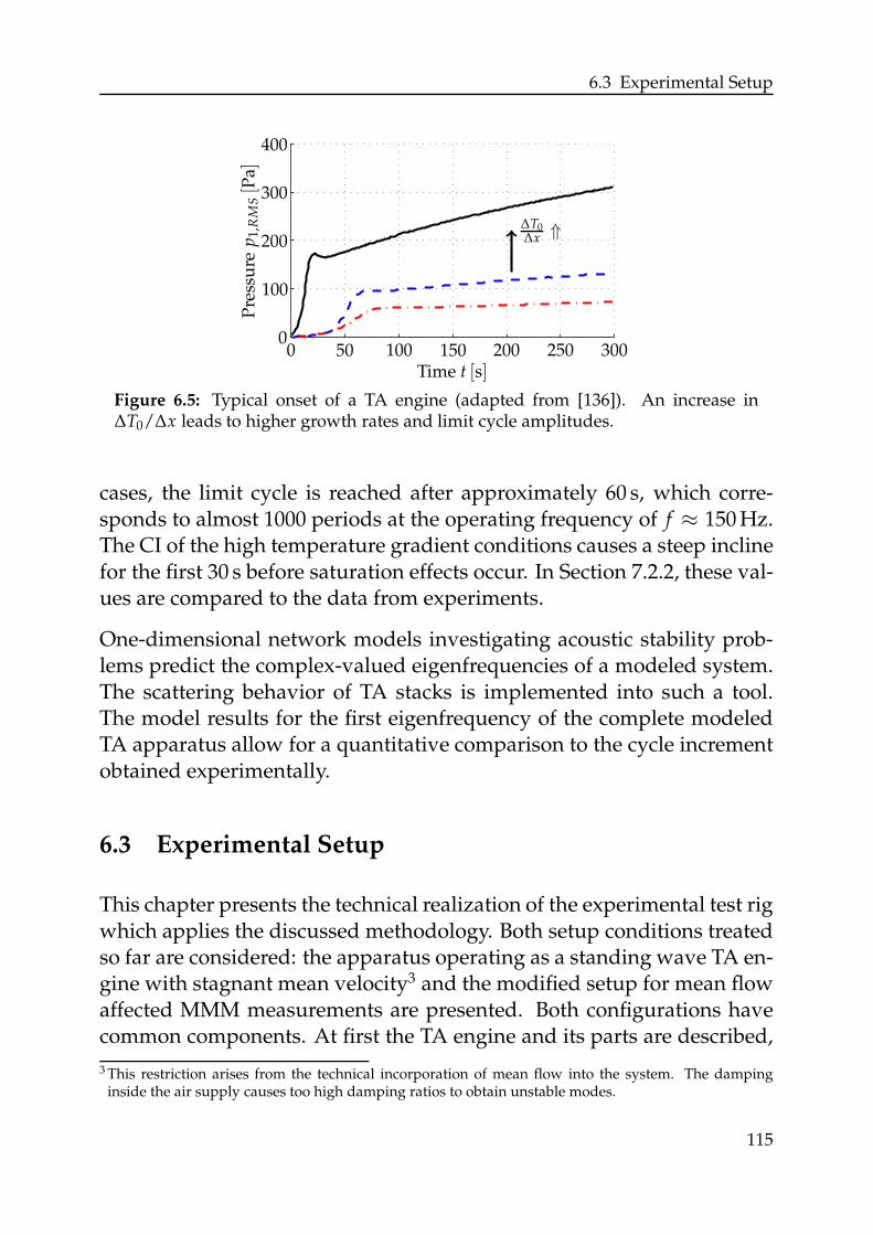
6.3 Experimental Setup
00
100
100
200
200
300
300
400
50 150 250Time t [s]
Pre
ssu
rep
1,R
MS[P
a]
∆T0∆x ⇑
Figure 6.5: Typical onset of a TA engine (adapted from [136]). An increase in∆T0/∆x leads to higher growth rates and limit cycle amplitudes.
cases, the limit cycle is reached after approximately 60 s, which corre-sponds to almost 1000 periods at the operating frequency of f ≈ 150 Hz.The CI of the high temperature gradient conditions causes a steep inclinefor the first 30 s before saturation effects occur. In Section 7.2.2, these val-ues are compared to the data from experiments.
One-dimensional network models investigating acoustic stability prob-lems predict the complex-valued eigenfrequencies of a modeled system.The scattering behavior of TA stacks is implemented into such a tool.The model results for the first eigenfrequency of the complete modeledTA apparatus allow for a quantitative comparison to the cycle incrementobtained experimentally.
6.3 Experimental Setup
This chapter presents the technical realization of the experimental test rigwhich applies the discussed methodology. Both setup conditions treatedso far are considered: the apparatus operating as a standing wave TA en-gine with stagnant mean velocity3 and the modified setup for mean flowaffected MMM measurements are presented. Both configurations havecommon components. At first the TA engine and its parts are described,
3 This restriction arises from the technical incorporation of mean flow into the system. The dampinginside the air supply causes too high damping ratios to obtain unstable modes.
115
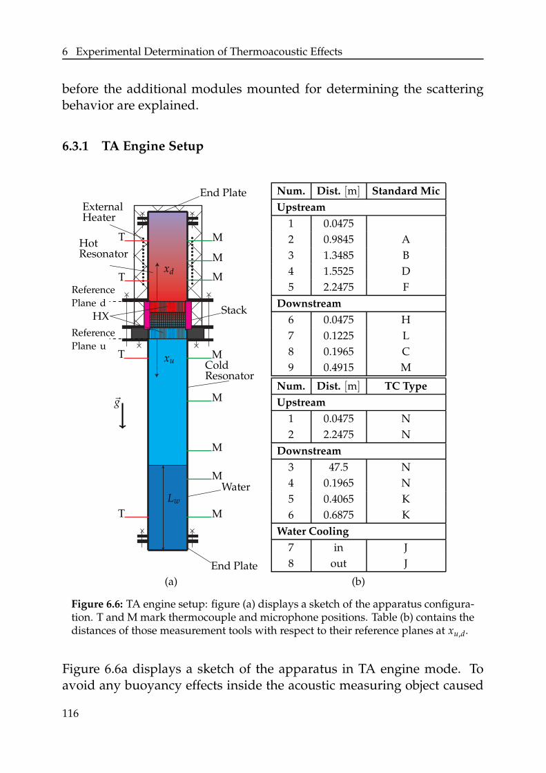
6 Experimental Determination of Thermoacoustic Effects
before the additional modules mounted for determining the scatteringbehavior are explained.
6.3.1 TA Engine Setup
T
T
T
T
M
M
M
M
M
M
M
M
StackHX
Water
xu
xd
Lw
ColdResonator
HotResonator
ExternalHeater
End Plate
End Plate
Reference
Plane u
Reference
Plane d
~g
(a)
Num. Dist. [m] Standard Mic
Upstream
1 0.0475
2 0.9845 A
3 1.3485 B
4 1.5525 D
5 2.2475 F
Downstream
6 0.0475 H
7 0.1225 L
8 0.1965 C
9 0.4915 M
Num. Dist. [m] TC Type
Upstream
1 0.0475 N
2 2.2475 N
Downstream
3 47.5 N
4 0.1965 N
5 0.4065 K
6 0.6875 K
Water Cooling
7 in J
8 out J
(b)
Figure 6.6: TA engine setup: figure (a) displays a sketch of the apparatus configura-tion. T and M mark thermocouple and microphone positions. Table (b) contains thedistances of those measurement tools with respect to their reference planes at xu,d.
Figure 6.6a displays a sketch of the apparatus in TA engine mode. Toavoid any buoyancy effects inside the acoustic measuring object caused
116
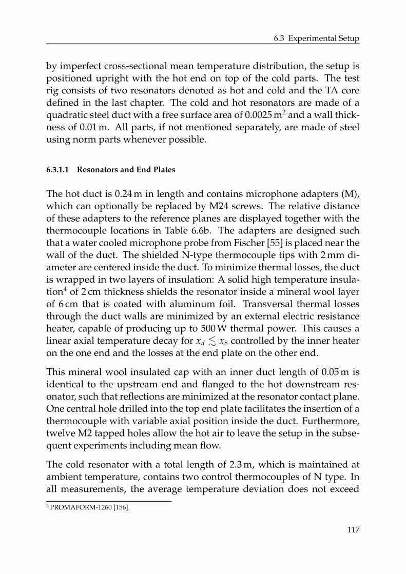
6.3 Experimental Setup
by imperfect cross-sectional mean temperature distribution, the setup ispositioned upright with the hot end on top of the cold parts. The testrig consists of two resonators denoted as hot and cold and the TA coredefined in the last chapter. The cold and hot resonators are made of aquadratic steel duct with a free surface area of 0.0025 m2 and a wall thick-ness of 0.01 m. All parts, if not mentioned separately, are made of steelusing norm parts whenever possible.
6.3.1.1 Resonators and End Plates
The hot duct is 0.24 m in length and contains microphone adapters (M),which can optionally be replaced by M24 screws. The relative distanceof these adapters to the reference planes are displayed together with thethermocouple locations in Table 6.6b. The adapters are designed suchthat a water cooled microphone probe from Fischer [55] is placed near thewall of the duct. The shielded N-type thermocouple tips with 2 mm di-ameter are centered inside the duct. To minimize thermal losses, the ductis wrapped in two layers of insulation: A solid high temperature insula-tion4 of 2 cm thickness shields the resonator inside a mineral wool layerof 6 cm that is coated with aluminum foil. Transversal thermal lossesthrough the duct walls are minimized by an external electric resistanceheater, capable of producing up to 500 W thermal power. This causes alinear axial temperature decay for xd . x8 controlled by the inner heateron the one end and the losses at the end plate on the other end.
This mineral wool insulated cap with an inner duct length of 0.05 m isidentical to the upstream end and flanged to the hot downstream res-onator, such that reflections are minimized at the resonator contact plane.One central hole drilled into the top end plate facilitates the insertion of athermocouple with variable axial position inside the duct. Furthermore,twelve M2 tapped holes allow the hot air to leave the setup in the subse-quent experiments including mean flow.
The cold resonator with a total length of 2.3 m, which is maintained atambient temperature, contains two control thermocouples of N type. Inall measurements, the average temperature deviation does not exceed
4 PROMAFORM-1260 [156].
117
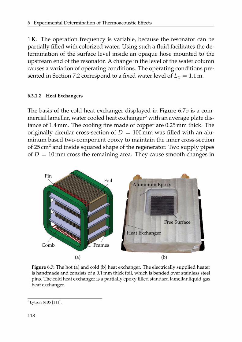
6 Experimental Determination of Thermoacoustic Effects
1 K. The operation frequency is variable, because the resonator can bepartially filled with colorized water. Using such a fluid facilitates the de-termination of the surface level inside an opaque hose mounted to theupstream end of the resonator. A change in the level of the water columncauses a variation of operating conditions. The operating conditions pre-sented in Section 7.2 correspond to a fixed water level of Lw = 1.1 m.
6.3.1.2 Heat Exchangers
The basis of the cold heat exchanger displayed in Figure 6.7b is a com-mercial lamellar, water cooled heat exchanger5 with an average plate dis-tance of 1.4 mm. The cooling fins made of copper are 0.25 mm thick. Theoriginally circular cross-section of D = 100 mm was filled with an alu-minum based two-component epoxy to maintain the inner cross-sectionof 25 cm2 and inside squared shape of the regenerator. Two supply pipesof D = 10 mm cross the remaining area. They cause smooth changes in
700
PinFoil
Comb Frames
(a)
Aluminum Epoxy
Heat Exchanger
Free Surface
(b)
Figure 6.7: The hot (a) and cold (b) heat exchanger. The electrically supplied heateris handmade and consists of a 0.1 mm thick foil, which is bended over stainless steelpins. The cold heat exchanger is a partially epoxy filled standard lamellar liquid-gasheat exchanger.
5 Lytron 6105 [111].
118
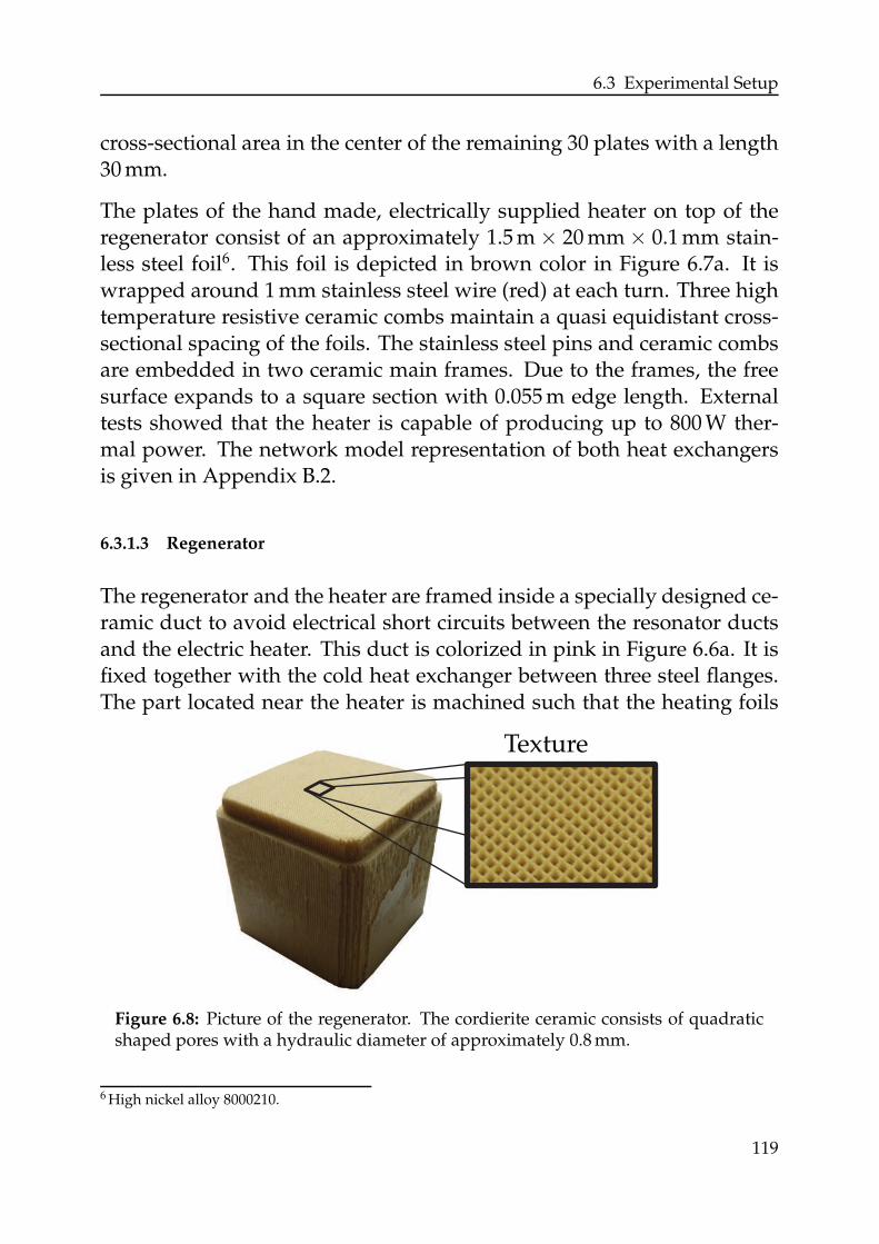
6.3 Experimental Setup
cross-sectional area in the center of the remaining 30 plates with a length30 mm.
The plates of the hand made, electrically supplied heater on top of theregenerator consist of an approximately 1.5 m × 20 mm × 0.1 mm stain-less steel foil6. This foil is depicted in brown color in Figure 6.7a. It iswrapped around 1 mm stainless steel wire (red) at each turn. Three hightemperature resistive ceramic combs maintain a quasi equidistant cross-sectional spacing of the foils. The stainless steel pins and ceramic combsare embedded in two ceramic main frames. Due to the frames, the freesurface expands to a square section with 0.055 m edge length. Externaltests showed that the heater is capable of producing up to 800 W ther-mal power. The network model representation of both heat exchangersis given in Appendix B.2.
6.3.1.3 Regenerator
The regenerator and the heater are framed inside a specially designed ce-ramic duct to avoid electrical short circuits between the resonator ductsand the electric heater. This duct is colorized in pink in Figure 6.6a. It isfixed together with the cold heat exchanger between three steel flanges.The part located near the heater is machined such that the heating foils
Texture
Figure 6.8: Picture of the regenerator. The cordierite ceramic consists of quadraticshaped pores with a hydraulic diameter of approximately 0.8 mm.
6 High nickel alloy 8000210.
119
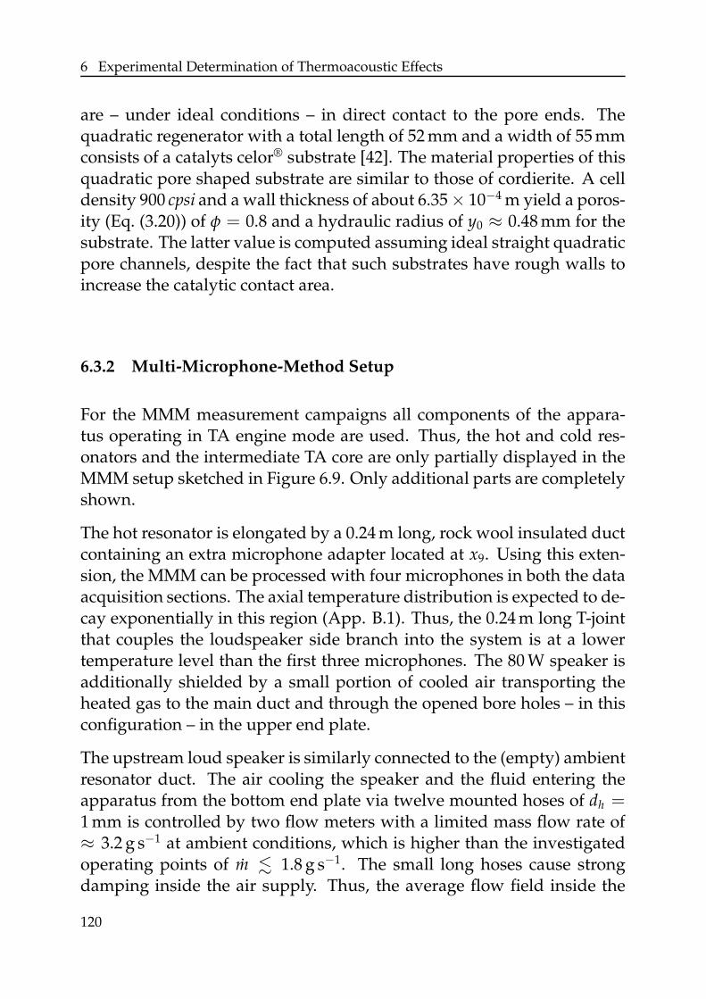
6 Experimental Determination of Thermoacoustic Effects
are – under ideal conditions – in direct contact to the pore ends. Thequadratic regenerator with a total length of 52 mm and a width of 55 mmconsists of a catalyts celor® substrate [42]. The material properties of thisquadratic pore shaped substrate are similar to those of cordierite. A celldensity 900 cpsi and a wall thickness of about 6.35 × 10⁻⁴ m yield a poros-ity (Eq. (3.20)) of φ = 0.8 and a hydraulic radius of y0 ≈ 0.48 mm for thesubstrate. The latter value is computed assuming ideal straight quadraticpore channels, despite the fact that such substrates have rough walls toincrease the catalytic contact area.
6.3.2 Multi-Microphone-Method Setup
For the MMM measurement campaigns all components of the appara-tus operating in TA engine mode are used. Thus, the hot and cold res-onators and the intermediate TA core are only partially displayed in theMMM setup sketched in Figure 6.9. Only additional parts are completelyshown.
The hot resonator is elongated by a 0.24 m long, rock wool insulated ductcontaining an extra microphone adapter located at x9. Using this exten-sion, the MMM can be processed with four microphones in both the dataacquisition sections. The axial temperature distribution is expected to de-cay exponentially in this region (App. B.1). Thus, the 0.24 m long T-jointthat couples the loudspeaker side branch into the system is at a lowertemperature level than the first three microphones. The 80 W speaker isadditionally shielded by a small portion of cooled air transporting theheated gas to the main duct and through the opened bore holes – in thisconfiguration – in the upper end plate.
The upstream loud speaker is similarly connected to the (empty) ambientresonator duct. The air cooling the speaker and the fluid entering theapparatus from the bottom end plate via twelve mounted hoses of dh =1 mm is controlled by two flow meters with a limited mass flow rate of≈ 3.2 g s−1 at ambient conditions, which is higher than the investigatedoperating points of m . 1.8 g s−1. The small long hoses cause strongdamping inside the air supply. Thus, the average flow field inside the
120
6.3 Experimental Setup
T
T
T
T
M
M
M
TA Engine Setup
ColdAir
HotAir
SpeakerCooling
ColdResonator
HotResonator
IntermediateDuct
SpeakerT-Joint
SpeakerT-Joint
Loudspeaker
Loudspeaker
End Plate
End Plate
Figure 6.9: Sketch of the MMM setup. Those parts of the apparatus that are alsoused in the TA engine setup are omitted. Both resonators are supplied by a speakerthat is mounted in combination with a T-joint. For data acquisition purposes, the hotresonator is elongated by an isolated duct. In case of mean flow, the flow directionpoints from the bottom to the top.
measurement setup is almost decoupled from the air supply upstream ofthe feeding hoses.
6.3.3 Measurement Processs
The thermocouples controlling the temperature distribution inside thesetup are connected to a cold-junction compensated external data ana-
121
6 Experimental Determination of Thermoacoustic Effects
lyzer7 reading all temperature values using a sampling rate of ∆t = 1 s.As soon as the collected parameters vary less than 5 K min−1, the state isassumed to be steady. The deviation of the stack outlet temperature tothe value of the first thermocouple behind the heater is lower than 5 Kfor the downstream stack temperature range of up to 500 K.
The analysis is conducted over a frequency range of 5 Hz to 600 Hz inconstant steps of 5 Hz. The speakers drive the acoustic field inside thesetup for a minimum of 3 times the data acquisition period at each fre-quency. The excitation amplitude is controlled by a preliminary equal-izing loop, whereas the maximum measured pressure magnitude ob-tained for each frequency is calibrated to 30 ± 5 Pa. Due to the midrange characteristics of the speakers, especially the lowest frequenciesof 5 Hz ≤ f ≤ 25 Hz can not be maintained at this level. Each data ac-quisition loop is followed by an idle time of several seconds to ensureundisturbed initial conditions.
The signals obtained from the pressure sensors – here capacitive micro-phones [65] are used – are amplified to 1 mV Pa−1 before they are readout by a sequential AD interface card at a sampling rate of 8000 s−1, lead-ing to a temporal resolution of more than 12 points for the maximuminvestigated frequency of 600 Hz.
The time series are band pass filtered and transformed to frequency spaceusing an FFT-algorithm. The peak frequency data detected in the fre-quency band of ±5 Hz around the current frequency of excitation arestored for later post-processing. A calibration process similar to Fischer[55] compensates the impact of the sequential data acquisition delay.
6.3.3.1 Quality Estimations
Abom and Boden [4, 27], demonstrated that the achieved measurementquality is sensitive to various issues. As shown by Fischer [55], all param-eters influencing the data fitting process are crucial for obtaining accurateresults. This section discusses the preliminary quality predictions for themeasurement method. Estimations from literature as well as considera-tions of problem-dependent error impacts are presented.7 Agilent 34970A [6].
122
6.3 Experimental Setup
The intended analytical temperature distribution based on up to 4 localsensors seems to be a rough estimate. The profile affects the acoustictransport in two ways: some parts of the characteristic waves are re-flected with the factor Θ−1
2 at the approximated temperature changes, andthe actual k± (Eq. (3.28)) inside the duct is modified by the temperature-dependent speed of sound. Both, the reflection error and the error in
transport speed scale with ±√
∆TT
. This leads to an error impact of less
than 1% in the final computation of the scattering matrices.
Due to the direct impact on the fitting process, the MMM results are moresensitive to the acquired pressure data. The accuracy of these values de-pends on the signal to noise ratio, the microphone accuracy, the data ac-quisition system and the quality of the calibration coefficients.
The first and second errors can be reduced by repeatedly varying the mi-crophone positions [123] and averaging over several measurement cam-paigns. The calibration causes constant offset errors that sum up duringthe averaging process. As the calibration relies on the accuracy of thereference microphone8, the complete data set depends on the accuracy ofthis pressure sensor and the reproducibility of its data. The latter stronglydepends on the observed frequency. Measurements obtained from otherapplications revealed that data below 100 Hz [55] have to be consideredcarefully because the error exceeds a reliable range.
Due to the questionable reliability of the data, a cautious considerationof the statistics of the fitting process is necessary. Translating determineddeviations from the fitting in characteristic wave space into the scatteringmatrix notation is not straightforward. The dimensional error quantitiesof the least square fit method are not directly comparable to the errorin transmission prediction. Also, a non-dimensionalization by normaliz-ing the quantities with the computed characteristic wave amplitudes, orreference pressures, only leads to comparable results for traveling waveconditions. Such conditions occur if highly absorbing conditions at theopposite side of the acting speaker are generated. Processing all errorquantities and their combinations from the fitting procedure to the finalscattering matrix notation is very time consuming and increase the re-
8 Here microphone M is chosen.
123
6 Experimental Determination of Thermoacoustic Effects
quired active storage. Thus, a different approach is used to determine aquality measure for the scattering matrix obtained experimentally. Thismethod is inspired by the bootstrapping technique [14] applied to theCFD/SI method by Foeller [57] and Tay [192]. It uses random parts ofsignals to find confidence intervals for the results. In contrast to the boot-strapping technique, the data is considered in the frequency domain. Fur-ther, all possible data sets and no random selection is used. The ideais to fit the mode shape to a reduced number of pressure sensors bysequentially removing some microphone data columns from the fittingprocess. A stochastic analysis of all resulting reference wave amplitudesleads to a complex-valued variation in the determined scattering matrixcoefficients. Summing up over all possible combinations leads to a meanvalue, which is identical to the fit achieved by taking all data into ac-count. Moreover, statistical data like standard deviation and maximumerror are computed from these results. As these data are dimensionless,their magnitude is a comparable measure for the accuracy of the data.These values are plotted in terms of error bars in the experimentally de-termined scattering matrices presented in Section 7.1.4.3.
124
7 Thermoacoustic Interaction in Zero MeanFlow Conditions
This thesis uses and cross-validates three different methods to investigatethe TA effect. The cross-sectionally averaged scattering behavior is con-sidered experimentally, semi-analytically and by the application of multi-dimensional CFD simulations. The methods used are validated for stag-nant mean flow conditions and the accuracy of the different approachesis discussed in Section 7.1. The application of the predicted scattering be-havior is used in the second section to show the predictability of typicaloperating conditions of the experimental setup in the TA engine mode.An investigation of the instability potentiality of the reference test caseconcludes the present chapter. Due to its low computational costs, theone-dimensional model approach derived in Chapter 4 facilitates a pa-rameter variation in terms of this potentiality. The IP of deviating meanparameter provides an insight into the capabilities for different configu-rations.
7.1 Scattering Behavior of Thermoacoustic Stacks
This section presents the scattering matrices obtained by experimentaldata (EXP), one-dimensional numerical modeling (IMP, MI and MII)and CFD/SI methods (CFD), respectively. For improved clarity in pre-senting the data graphically, the results of these three different ap-proaches are displayed separately in Sections 7.1.1 and 7.1.3. Further-more, in Section 7.1.2 it is shown that the results correspond to the pre-dictions of a simplistic analytical model in the limit of high frequencies.Finally, an error analysis of the methods applied is performed.
125
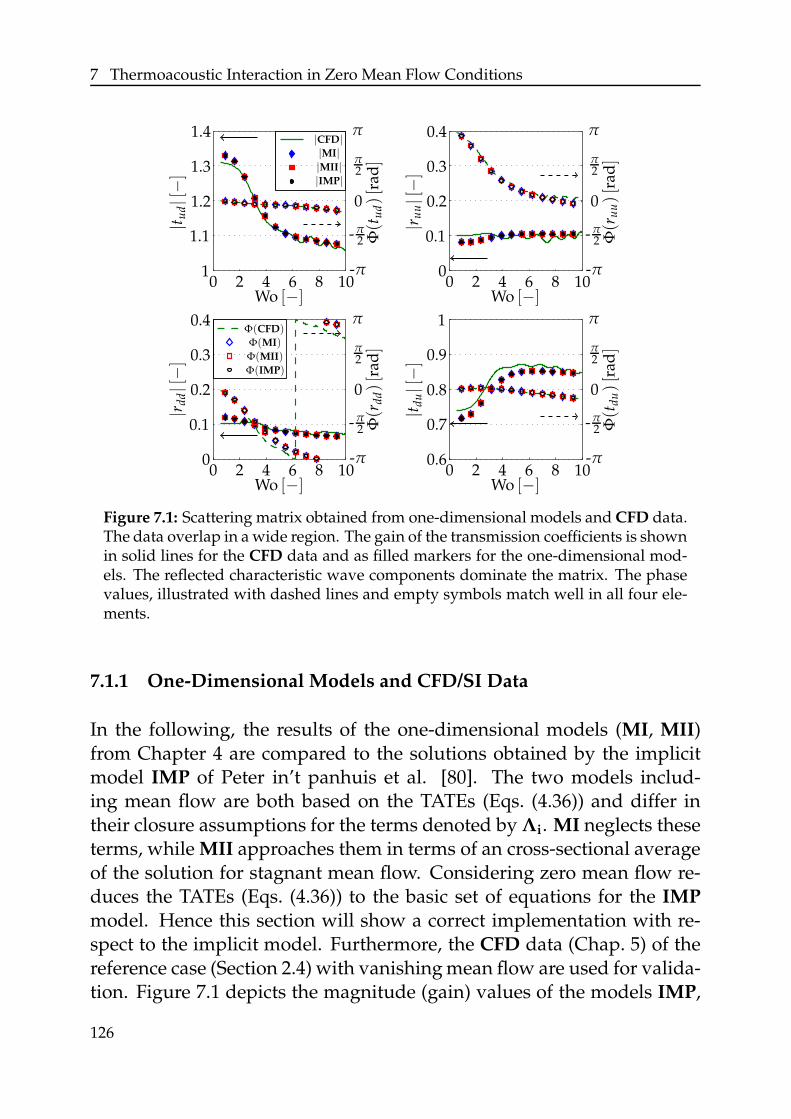
7 Thermoacoustic Interaction in Zero Mean Flow Conditions
000
000
1
1
22
22
44
44
66
66
88
88
1010
1010
0.1
0.1
0.2
0.2
0.3
0.3
0.4
0.4
0.6
0.7
0.8
0.9
1.1
1.2
1.3
1.4
Wo [−]Wo [−]
Wo [−]Wo [−]
|t ud|[−]
Φ(t
ud)[r
ad]
|t du|[−]
Φ(t
du)[r
ad]
|r dd|[−]
Φ(r
dd)[r
ad]
|r uu|[−]
Φ(r
uu)[r
ad]
ππ
ππ
π2
π2
π2
π2
00
00
-π2-π
2
-π2-π
2
-π-π
-π-π
|CFD|
Φ(CFD)
|MI|
Φ(MI)
|MII|
Φ(MII)
|IMP|
Φ(IMP)
Figure 7.1: Scattering matrix obtained from one-dimensional models and CFD data.The data overlap in a wide region. The gain of the transmission coefficients is shownin solid lines for the CFD data and as filled markers for the one-dimensional mod-els. The reflected characteristic wave components dominate the matrix. The phasevalues, illustrated with dashed lines and empty symbols match well in all four ele-ments.
7.1.1 One-Dimensional Models and CFD/SI Data
In the following, the results of the one-dimensional models (MI, MII)from Chapter 4 are compared to the solutions obtained by the implicitmodel IMP of Peter in’t panhuis et al. [80]. The two models includ-ing mean flow are both based on the TATEs (Eqs. (4.36)) and differ intheir closure assumptions for the terms denoted by Λi. MI neglects theseterms, while MII approaches them in terms of an cross-sectional averageof the solution for stagnant mean flow. Considering zero mean flow re-duces the TATEs (Eqs. (4.36)) to the basic set of equations for the IMP
model. Hence this section will show a correct implementation with re-spect to the implicit model. Furthermore, the CFD data (Chap. 5) of thereference case (Section 2.4) with vanishing mean flow are used for valida-tion. Figure 7.1 depicts the magnitude (gain) values of the models IMP,
126
7.1 Scattering Behavior of Thermoacoustic Stacks
MI and MII with filled symbols. The gain obtained from the CFD/SImethod is displayed by a green solid curve. All these values scale withthe left-hand side vertical axis of the four plots in Figure 7.1. The blanksymbols represent the phase values of the model data, scaling with theright-hand side vertical axis. The color and shape are the same as forits magnitude value. The dashed line describes the phase values of theCFD. For reasons of generality, all data are plotted versus the Womers-ley number Wo of the reference (cold) side. As stated in Section 4.2, Wo isproportional to the hydraulic radius and the square root of the frequency.The transformation from this space into the Lautrec number La space islinear (Eq. (4.7)) and provides similar insight.
The gain and phase values of the transmission coefficients tud, tdu aswell as the reflection coefficients ruu, rdd displayed in Figure 7.1 matchvery well. As expected, all one-dimensional modeling approaches pre-dict identical scattering values. Both phases Φ(tud) and Φ(tdu) of CFD
and these models completely overlap in the displayed range. This alsoaccounts for the phase of the characteristic wave reflected at the cold up-stream side. Only the reflected hot wave phase Φ(rdd) deviates percep-tibly for Wo > 6, but is acceptable because of the corresponding gainvalue.
Concerning the magnitude values of the scattering matrix coefficients,two observations can be made:
• In contrast to the one-dimensional models, the CFD solution forhigher frequencies contains wiggles. These are artificial productsof the SI [58] (also Fig. 7.4). Considering the one-dimensional modelof Rott [170], these wiggles are not reproducible by the steady de-caying Rott functions (Eqs. (7.8)) displayed in Swift’s textbook [187].Approximating this region by a polynomial least-square fit shouldresult in an accurate match with the one-dimensional model data.
• At low frequencies (Wo < 1), the CFD solution tends to underes-timate the TA interaction. The transmission coefficients are closerto unity and the corresponding characteristic wave is amplified lesswith a maximum gain deviation of 0.02 in the low Wo limit of tud.The low frequency region of the reflection coefficients experiences a
127
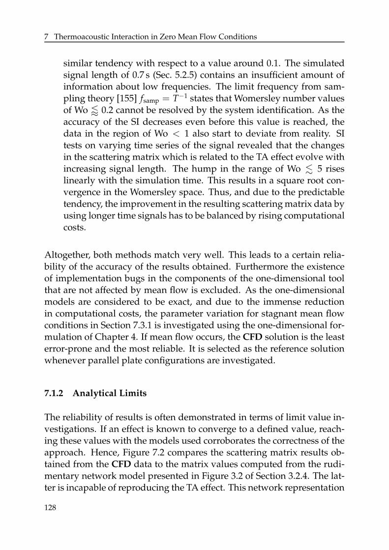
7 Thermoacoustic Interaction in Zero Mean Flow Conditions
similar tendency with respect to a value around 0.1. The simulatedsignal length of 0.7 s (Sec. 5.2.5) contains an insufficient amount ofinformation about low frequencies. The limit frequency from sam-pling theory [155] fsamp = T−1 states that Womersley number valuesof Wo / 0.2 cannot be resolved by the system identification. As theaccuracy of the SI decreases even before this value is reached, thedata in the region of Wo < 1 also start to deviate from reality. SItests on varying time series of the signal revealed that the changesin the scattering matrix which is related to the TA effect evolve withincreasing signal length. The hump in the range of Wo . 5 riseslinearly with the simulation time. This results in a square root con-vergence in the Womersley space. Thus, and due to the predictabletendency, the improvement in the resulting scattering matrix data byusing longer time signals has to be balanced by rising computationalcosts.
Altogether, both methods match very well. This leads to a certain relia-bility of the accuracy of the results obtained. Furthermore the existenceof implementation bugs in the components of the one-dimensional toolthat are not affected by mean flow is excluded. As the one-dimensionalmodels are considered to be exact, and due to the immense reductionin computational costs, the parameter variation for stagnant mean flowconditions in Section 7.3.1 is investigated using the one-dimensional for-mulation of Chapter 4. If mean flow occurs, the CFD solution is the leasterror-prone and the most reliable. It is selected as the reference solutionwhenever parallel plate configurations are investigated.
7.1.2 Analytical Limits
The reliability of results is often demonstrated in terms of limit value in-vestigations. If an effect is known to converge to a defined value, reach-ing these values with the models used corroborates the correctness of theapproach. Hence, Figure 7.2 compares the scattering matrix results ob-tained from the CFD data to the matrix values computed from the rudi-mentary network model presented in Figure 3.2 of Section 3.2.4. The lat-ter is incapable of reproducing the TA effect. This network representation
128
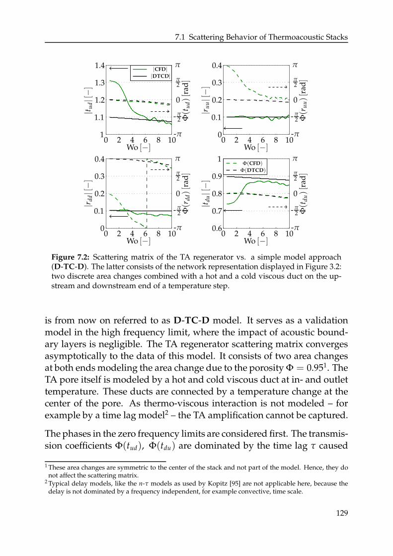
7.1 Scattering Behavior of Thermoacoustic Stacks
000
000
1
1
22
22
44
44
66
66
88
88
1010
1010
0.1
0.1
0.2
0.2
0.3
0.3
0.4
0.4
0.6
0.7
0.8
0.9
1.1
1.2
1.3
1.4
Wo [−]Wo [−]
Wo [−]Wo [−]
|t ud|[−]
Φ(t
ud)[r
ad]
|t du|[−]
Φ(t
du)[r
ad]
|r dd|[−]
Φ(r
dd)[r
ad]
|r uu|[−]
Φ(r
uu)[r
ad]
ππ
ππ
π2
π2
π2
π2
00
00
-π2-π
2
-π2-π
2
-π-π
-π-π
|CFD|
Φ(CFD)
|DTCD|
Φ(DTCD)
Figure 7.2: Scattering matrix of the TA regenerator vs. a simple model approach(D-TC-D). The latter consists of the network representation displayed in Figure 3.2:two discrete area changes combined with a hot and a cold viscous duct on the up-stream and downstream end of a temperature step.
is from now on referred to as D-TC-D model. It serves as a validationmodel in the high frequency limit, where the impact of acoustic bound-ary layers is negligible. The TA regenerator scattering matrix convergesasymptotically to the data of this model. It consists of two area changesat both ends modeling the area change due to the porosity Φ = 0.951. TheTA pore itself is modeled by a hot and cold viscous duct at in- and outlettemperature. These ducts are connected by a temperature change at thecenter of the pore. As thermo-viscous interaction is not modeled – forexample by a time lag model2 – the TA amplification cannot be captured.
The phases in the zero frequency limits are considered first. The transmis-sion coefficients Φ(tud), Φ(tdu) are dominated by the time lag τ caused
1 These area changes are symmetric to the center of the stack and not part of the model. Hence, they donot affect the scattering matrix.
2 Typical delay models, like the n-τ models as used by Kopitz [95] are not applicable here, because thedelay is not dominated by a frequency independent, for example convective, time scale.
129
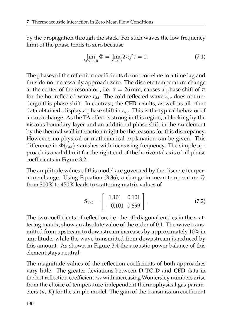
7 Thermoacoustic Interaction in Zero Mean Flow Conditions
by the propagation through the stack. For such waves the low frequencylimit of the phase tends to zero because
limWo → 0
Φ = limf → 0
2π f τ = 0. (7.1)
The phases of the reflection coefficients do not correlate to a time lag andthus do not necessarily approach zero. The discrete temperature changeat the center of the resonator , i.e. x = 26 mm, causes a phase shift of πfor the hot reflected wave rdd. The cold reflected wave ruu does not un-dergo this phase shift. In contrast, the CFD results, as well as all otherdata obtained, display a phase shift in ruu. This is the typical behavior ofan area change. As the TA effect is strong in this region, a blocking by theviscous boundary layer and an additional phase shift in the rdd elementby the thermal wall interaction might be the reasons for this discrepancy.However, no physical or mathematical explanation can be given. Thisdifference in Φ(rdd) vanishes with increasing frequency. The simple ap-proach is a valid limit for the right end of the horizontal axis of all phasecoefficients in Figure 3.2.
The amplitude values of this model are governed by the discrete temper-ature change. Using Equation (3.36), a change in mean temperature T0
from 300 K to 450 K leads to scattering matrix values of
STC =
[
1.101 0.101
−0.101 0.899
]
. (7.2)
The two coefficients of reflection, i.e. the off-diagonal entries in the scat-tering matrix, show an absolute value of the order of 0.1. The wave trans-mitted from upstream to downstream increases by approximately 10% inamplitude, while the wave transmitted from downstream is reduced bythis amount. As shown in Figure 3.4 the acoustic power balance of thiselement stays neutral.
The magnitude values of the reflection coefficients of both approachesvary little. The greater deviations between D-TC-D and CFD data inthe hot reflection coefficient rdd with increasing Womersley numbers arisefrom the choice of temperature-independent thermophysical gas param-eters (µ, K) for the simple model. The gain of the transmission coefficient
130
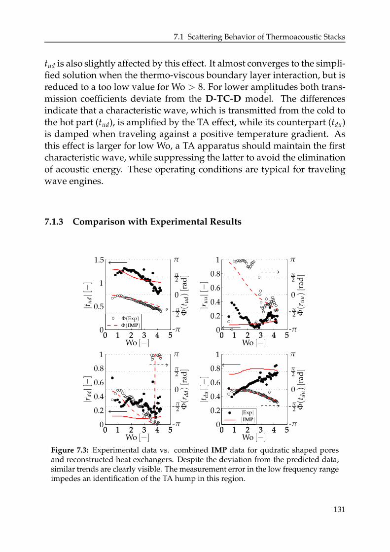
7.1 Scattering Behavior of Thermoacoustic Stacks
tud is also slightly affected by this effect. It almost converges to the simpli-fied solution when the thermo-viscous boundary layer interaction, but isreduced to a too low value for Wo > 8. For lower amplitudes both trans-mission coefficients deviate from the D-TC-D model. The differencesindicate that a characteristic wave, which is transmitted from the cold tothe hot part (tud), is amplified by the TA effect, while its counterpart (tdu)is damped when traveling against a positive temperature gradient. Asthis effect is larger for low Wo, a TA apparatus should maintain the firstcharacteristic wave, while suppressing the latter to avoid the eliminationof acoustic energy. These operating conditions are typical for travelingwave engines.
7.1.3 Comparison with Experimental Results
00
00
00
00
00
00
11
11
1
1
1
1
1
1
1
1
22
22
22
22
33
33
33
33
44
44
44
44
55
55
55
55
0.20.2
0.2
0.40.4
0.40.5
0.60.6
0.6
0.80.8
0.8
1.5
Wo [−]Wo [−]
Wo [−]Wo [−]
|t ud|[−]
Φ(t
ud)[r
ad]
|t du|[−]
Φ(t
du)[r
ad]
|r dd|[−]
Φ(r
dd)[r
ad]
|r uu|[−]
Φ(r
uu)[r
ad]
ππ
ππ
π2
π2
π2
π2
00
00
-π2-π
2
-π2-π
2
-π-π
-π-π
|IMP|
Φ(IMP)
|Exp|
Φ(Exp)
Figure 7.3: Experimental data vs. combined IMP data for qudratic shaped poresand reconstructed heat exchangers. Despite the deviation from the predicted data,similar trends are clearly visible. The measurement error in the low frequency rangeimpedes an identification of the TA hump in this region.
131
7 Thermoacoustic Interaction in Zero Mean Flow Conditions
Although detailed accurate numerical simulations usually describe thephysics with high reliability, experimental data are considered to be mostcredible. Figure 7.3 depicts the data obtained for the complete TA core bythe MMM presented in Section 6.1. The filled dots designate the mea-sured gain values, while the blank circles describe the phase. These dataare compared to the IMP results. These are manipulated using the re-constructed scattering matrices of the heat exchangers (Sec. 6.1.3). Here,the IMP results are obtained by inserting the proper Rott functions forquadratic shaped pores. While CFD and IMP of slab stacks match wellfor zero mean flow, choosing the latter reduces the error impact inducedby differences in cross-sectional geometry.
The measured phase of the transmission coefficients match very well fora wide region. This is due to the corresponding delay being governedby the timescale of the wave traveling through the media without anyinterference. The high frequency data are also in good agreement withthe reference data. Contrarily there is a huge mismatch for the scatter-ing matrix coefficients for Wo . 2. In comparison to the IMP data, theexperimental setup experiences a certain blocking that increases for lowfrequencies. Parts of the characteristic waves are reflected and thus in-crease the contribution of |r| while the transmission coefficient gains |t|are reduced. This frequency dependent reflectivity is not accounted forby analytical models of discrete area or temperature changes. Thus it cannot be reproduced in the reconstruction model of the heat exchangers.Swift [187] discusses the impact of wall roughness on the TA boundarylayer interaction. He observes that especially for rough walls the im-pact of viscous dissipation and, in a similar manner, thermal diffusionincreases. This effect can also be attributed to a partial blocking of theregenerator pores leading to a stronger reflection at low frequencies. Asecond reason for these contrary tendencies is due to the applied pres-sure sensors. As stated in Section 6.3.3.1, the capacitive signal conversiontechnique is sensitive to frequency. Low frequency data are affected bynon-statistical errors. This low Wo region is expected to be influenced byunidentified impacts and measurement errors. They impede a quantita-tive comparison to the data obtained numerically.
Nevertheless, the phase of the reflection coefficient Φ(ruu), which doesnot coincide with the D-TC-D model discussed in the last chapter, occurs
132
7.1 Scattering Behavior of Thermoacoustic Stacks
in a similar manner. Furthermore, the TA amplification in |tud| is stillvisible. In the next chapter, the author focuses on tendencies that theeffects experience when experimental data is affected by mean flow. Onlythese tendencies are taken into consideration.
7.1.4 Accuracy of Applied Methods
In the last chapter, three different methods for obtaining the scatteringmatrix of a TA regenerator were compared. Regardless of the good qual-itative agreement, these results have to be verified and validated becauseof the lack of comparable data in the published literature. Thus, thischapter discusses model and measurement errors as well as the accuracyof the techniques applied.
In contrast to the domains considered with the numerical tools, the ex-perimental setup investigates the real physical TA regenerator. Thus er-rors stemming from inadequate model assumptions of the regeneratordo not affect this measurement. However, the modeling approaches ofthe MMM procedure, the approximated geometry and its thermal fieldnevertheless induce a certain potential of model error.
The numerically investigated domains on the other hand are simplifiedwith respect to the technical device. No inlet/outlet interference like theformation of jets at the expansion or streaming effects are considered.Also the assumed axial mean temperature profile inside the regenera-tor is independent of losses to the exterior. In contrast to the approx-imated data of the one-dimensional models, all mean data is availablefrom the CFD simulation. Some error impact is related to the geomet-ric restriction of the investigated computational domain. As stated inSection 2.4, the influence of the openings and multi-dimensional effectsare not captured by the two-dimensional consideration of a single pore.Furthermore, buoyancy is a priori neglected. As the error impact of theapproaches arises from different sources, a quantitative comparison isimpossible. Determining the error impact of elements of the methods ap-plied and thereby obtaining a certain credibility of the acquired data isthe only way of supporting the cross-validation and verifying the choiceof the reference method.
133
7 Thermoacoustic Interaction in Zero Mean Flow Conditions
7.1.4.1 Quasi One-dimensional Modeling
The quasi-one-dimensional model of Rott [170] was shown to be exact forlong pores and for stagnant mean conditions by in’t panhuis et al. [81].Following the derivation of Chapter 4 and neglecting u for a pore withvanishing ratio of length scales ε, the resulting mathematical descriptionof the acoustic transport is exact for ideal conditions. As long as the meanflow is a quantity of second order and the pore is not affected by anylosses, which are not considered here, the modeling approach describedin this thesis is still valid. For stagnant mean flow conditions, all errorsin scattering matrix data are related to the numerical discretization andprovided thermophysical material data. The high accurate integrationscheme in combination with a step size of 10−5 yields a very precise re-sult. Thus, the tabulated data, which are stored with a precision of 10−4,induce the largest errors of similar magnitude into the equations.
Due to the restrictive assumptions mentioned, this high accuracy is onlyvalid for the stagnant mean flow case. As soon as m > 0, the error,which clearly stems from false closure assumptions, increases. Quanti-fying the accuracy is restricted to a comparison to data obtained by otherapproaches.
7.1.4.2 CFD and SI
The CFD simulation reveals a good agreement with the IMP model (seeFigure 7.1). As the configuration considered exactly matches the BCs ofthe 1D problem, the modeling error is supposed to be of the same or-der of magnitude. Entrance effects and inlet/outlet area changes are alsonot considered. Moreover, the temperature variation at the interface tothe solid material is not taken into account. As a laminar mean flowregime is considered, the impact of turbulent noise is negligible. Becausethe complete stack height in the experiment is two orders larger thanthe hydraulic pore radius (Sec. 6.3.1.3) and the conductivity of the fluidand the solid regenerator component are small in the experiment, inho-mogeneities due to losses to the exterior play a minor role. Thus, theseassumptions can be considered to introduce negligible error.
134
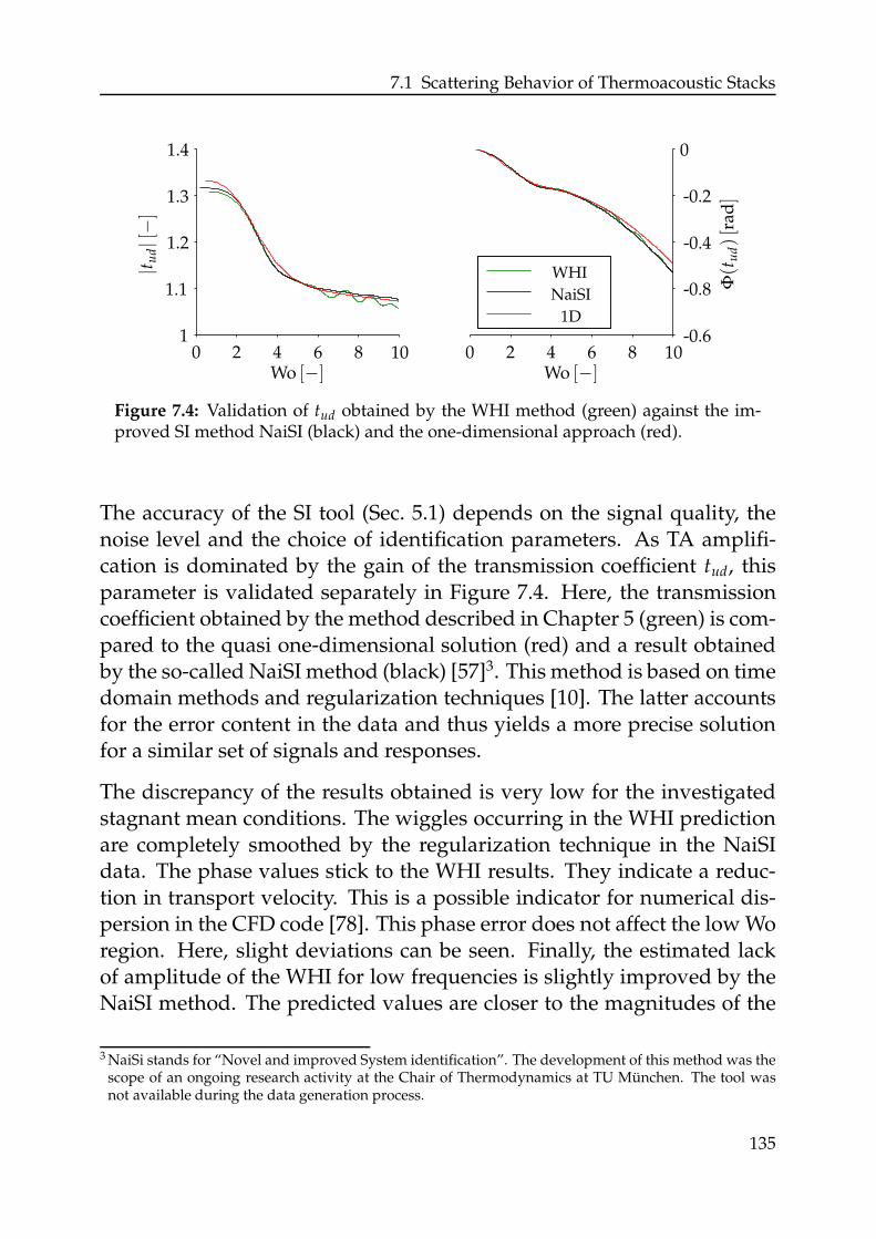
7.1 Scattering Behavior of Thermoacoustic Stacks
0
001
22 44 66 88 1010
-0.2
-0.4
1.1
1.2
1.3
1.4
Wo [−]Wo [−]
|t ud|[−]
Φ(t
ud)[r
ad]
-0.6
-0.8NaiSI
WHI
1D
Figure 7.4: Validation of tud obtained by the WHI method (green) against the im-proved SI method NaiSI (black) and the one-dimensional approach (red).
The accuracy of the SI tool (Sec. 5.1) depends on the signal quality, thenoise level and the choice of identification parameters. As TA amplifi-cation is dominated by the gain of the transmission coefficient tud, thisparameter is validated separately in Figure 7.4. Here, the transmissioncoefficient obtained by the method described in Chapter 5 (green) is com-pared to the quasi one-dimensional solution (red) and a result obtainedby the so-called NaiSI method (black) [57]3. This method is based on timedomain methods and regularization techniques [10]. The latter accountsfor the error content in the data and thus yields a more precise solutionfor a similar set of signals and responses.
The discrepancy of the results obtained is very low for the investigatedstagnant mean conditions. The wiggles occurring in the WHI predictionare completely smoothed by the regularization technique in the NaiSIdata. The phase values stick to the WHI results. They indicate a reduc-tion in transport velocity. This is a possible indicator for numerical dis-persion in the CFD code [78]. This phase error does not affect the low Woregion. Here, slight deviations can be seen. Finally, the estimated lackof amplitude of the WHI for low frequencies is slightly improved by theNaiSI method. The predicted values are closer to the magnitudes of the
3 NaiSi stands for “Novel and improved System identification”. The development of this method was thescope of an ongoing research activity at the Chair of Thermodynamics at TU Munchen. The tool wasnot available during the data generation process.
135
7 Thermoacoustic Interaction in Zero Mean Flow Conditions
1D values. However, as the time series is still too short, they cannot reachthis limit.
Summarizing, the WHI deviations in magnitude are up to 2% in the re-gion of the wiggles. The accuracy in the low frequency range is restrictedby the length of the investigated time series. All discrepancies resultfrom the SI errors and discretization errors4 in the CFD simulation. Thesediscrepancies are not related to mean flow and in combination with thequalitative agreement to the experimental data. The choice of the WHIsolution as reference data is justified.
7.1.4.3 Impacts of Measurement Error and Credibility of Experimental Data
The experimental data show larger deviations than other methods. Thus,the impact of possible errors is investigated in more detail.
Reconstruction Faults
The models applied and optimized for the consideration of the adjacentheat exchangers and geometrical changes inside the TA core are not per-fect. The parameters listed in Appendix B.2 allow only an approximatereconstruction of the acoustic scattering behavior of the heat exchang-ers. The assumed mean temperature profile T0(x) is computed usingfour measurement nodes. Moreover, as the error margins of numericaldata are of the same order as for the experimentally acquired data of theTA core, some effects may not be captured. If these are physical, butnot identifiable, their impact on the overall measured scattering behav-ior cannot be taken into account. The dominant decay and rise of themagnitude values of the scattering matrix data detected for Wo < 2 inFigure 7.3 is one of the three possibly uncaptured phenomena, whichmight be physical. A higher real viscous and thermal damping insidethe narrow geometries of the TA core could, on the one hand, cause astronger decay in the transmission coefficients |t|. On the other hand,it would affect both transmission coefficients in the same way for zero
4 In this context the discretization errors refer to the chosen discretization schemes and the numericaldispersion related to the solution techniques applied. Resolution errors from too coarse meshing ortime stepping are expected to play a less significant role.
136
7.1 Scattering Behavior of Thermoacoustic Stacks
mean velocity. This also accounts for the qualitative impact of losses dueto area changes. A further physical effect, which is not taken into account,is the strong reflection at low frequencies discussed in Section 7.1.3. Noacoustic element description is known to the author that predicts thisphenomenon and can be incorporated into the network representation ofthe reconstruction process.
Data Acquisition
The measurement chain for the MMM includes microphones, signal am-plifiers, an analog/digital interface and numerous cables and connectors.All these components contribute a certain error to the system. Abom andBoden [4] showed that the MMM is sensible to the accuracy of the mea-surement instrumentation as well as to the location of data acquisition.For the two-microphone method, they required a relative microphonedistance s of
0.1 < sπ(1 − Ma2)ω
c< 0.8, (7.3)
which is violated by a factor of up to approximately three. Here, the useof more than two microphones for the pressure fit balances this potentialerror source.
Especially the wiring connections and the pressure sensors are errorprone. These potentially systematic but unrepeatable errors can lead tonon-physical results notwithstanding a change of microphone orderingsand repeating the experiment [193]. Figure 7.5 depicts the relative ampli-tude and phase deviation of six (out of eight) microphones from the fittedpressure profiles over Womersley number for a) upstream and b) down-stream excitation. Each value displays the error of the microphone withrespect to the fitting through three microphones at each side, which areexemplarily depicted for a frequency of 140 Hz in Figure 6.3. These val-ues are non-dimensionalized by the acoustic pressure fit quantity that iscomputed for the ends of the TA core. Choosing a different set of micro-phones will lead to very similar results. The expected random deviationfor a stochastic amplitude and phase error only occurs for Womersleynumbers of Wo > 3. These values are larger than the rest. These errorsare balanced by the averaging procedure described in Section 6.3.3.1. In
137
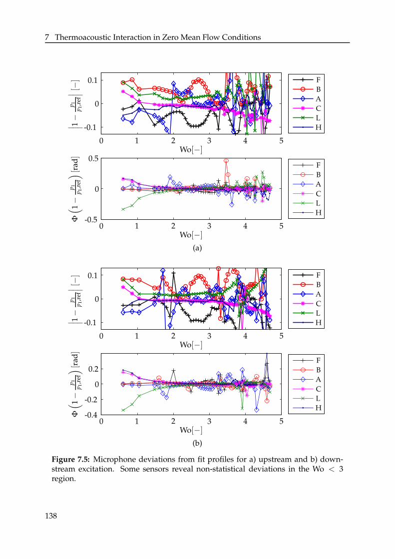
7 Thermoacoustic Interaction in Zero Mean Flow Conditions
Wo[−]
Wo[−]
∣ ∣ ∣1−
p1
p1,r
ef
∣ ∣ ∣[−
]Φ(
1−
p1
p1,r
ef
)
[rad
]
F
F
B
B
A
A
C
C
L
L
H
H
0
0
0
0
1
1
2
2
3
3
4
4
5
5
0.5
-0.5
0.1
-0.1
(a)
Wo[−]
Wo[−]
∣ ∣ ∣1−
p1
p1,r
ef
∣ ∣ ∣[−
]Φ(
1−
p1
p1,r
ef
)
[rad
]
F
F
B
B
A
A
C
C
L
L
H
H
0
0
0
0
1
1
2
2
3
3
4
4
5
5
0.1
-0.1
0.2
-0.2
-0.4
(b)
Figure 7.5: Microphone deviations from fit profiles for a) upstream and b) down-stream excitation. Some sensors reveal non-statistical deviations in the Wo < 3region.
138
7.1 Scattering Behavior of Thermoacoustic Stacks
contrast to this, almost all microphones display a clear trend to overes-timate (or respectively underestimate) the magnitude and phase whenthey fall below a certain frequency. Microphones B and L, for exam-ple, always record higher values than predicted by the fitted profile forWo < 3. This tendency of a consistent over- or underestimation can alsobe observed for the phase at low frequencies. The deviation is neitherlinked to the position of the active speaker nor to the microphone loca-tion. This trend in both quantities – gain and phase – is expressed interms of systematic errors in the scattering matrices that are not balancedby any averaging process. As the origin could not be identified by a vari-ation of the microphones and is not reproducible, the author expects thisdeviation to be part of the data acquisition system.
As discussed so far, an interpretation of the impact of the systematic erroron the scattering behavior is very difficult. Taking the microphone errorsinto account by weighing them in different variations does not lead toquantitative conclusions considering their impact on the predicted scat-tering matrix value. Hence, the method of predicting the scattering ma-trix values with varying combinations of microphone data (Sec. 6.3.3) ischosen. It is the only method to at least provide a qualitative estimate ofthe accuracy of the results obtained in terms of scattering matrix values.Using this method allows to determine statistical data as maximum errorand standard deviation, which are considered in the next section.
Measurement Errors
Figures 7.6 and 7.7 display the maximum error and standard deviation[91] of the measured zero mean flow scattering matrix. The eye-catchingdiscrepancy of the low frequency magnitudes (blue lines) supports thestatement that the accuracy of microphone measurements below 100 Hz5
is not satisfactory. Except for some frequencies the amplitude error de-creases with increasing Wo. These exceptions are not restricted to fluid-dynamic eigenfrequencies of the system. Observations during the mea-surement campaigns revealed that these deviations in the maximum er-ror and the standard deviation displayed in Figure 7.7 correspond to aresonance frequency of the complete setup. For these frequencies the ex-5 Wo < 1.64 in the present configuration.
139
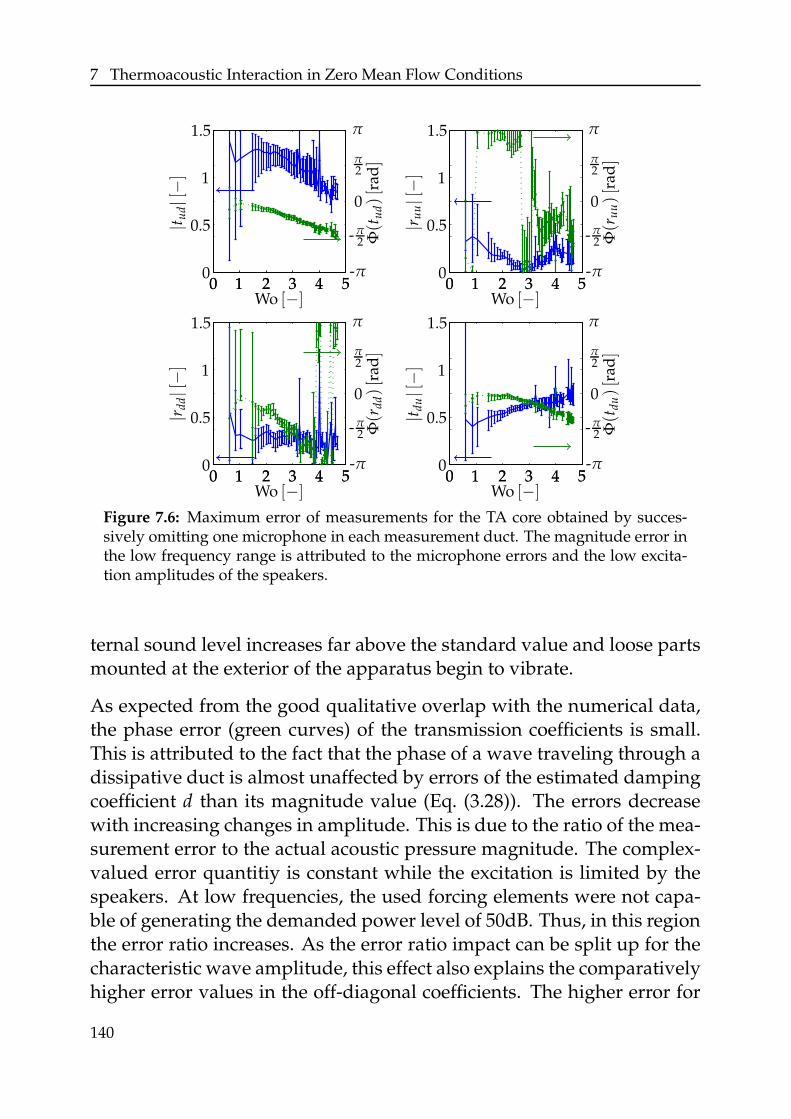
7 Thermoacoustic Interaction in Zero Mean Flow Conditions
0000
00
0000
00
1
1
11
1
1
1
1
11
1
1
2222
2222
3333
3333
4444
4444
5555
5555
0.50.5
0.50.5
1.51.5
1.51.5
Wo [−]Wo [−]
Wo [−]Wo [−]
|t ud|[−]
Φ(t
ud)[r
ad]
|t du|[−]
Φ(t
du)[r
ad]
|r dd|[−]
Φ(r
dd)[r
ad]
|r uu|[−]
Φ(r
uu)[r
ad]
ππ
ππ
π2
π2
π2
π2
00
00
-π2-π
2
-π2-π
2
-π-π
-π-π
Figure 7.6: Maximum error of measurements for the TA core obtained by succes-sively omitting one microphone in each measurement duct. The magnitude error inthe low frequency range is attributed to the microphone errors and the low excita-tion amplitudes of the speakers.
ternal sound level increases far above the standard value and loose partsmounted at the exterior of the apparatus begin to vibrate.
As expected from the good qualitative overlap with the numerical data,the phase error (green curves) of the transmission coefficients is small.This is attributed to the fact that the phase of a wave traveling through adissipative duct is almost unaffected by errors of the estimated dampingcoefficient d than its magnitude value (Eq. (3.28)). The errors decreasewith increasing changes in amplitude. This is due to the ratio of the mea-surement error to the actual acoustic pressure magnitude. The complex-valued error quantitiy is constant while the excitation is limited by thespeakers. At low frequencies, the used forcing elements were not capa-ble of generating the demanded power level of 50dB. Thus, in this regionthe error ratio increases. As the error ratio impact can be split up for thecharacteristic wave amplitude, this effect also explains the comparativelyhigher error values in the off-diagonal coefficients. The higher error for
140
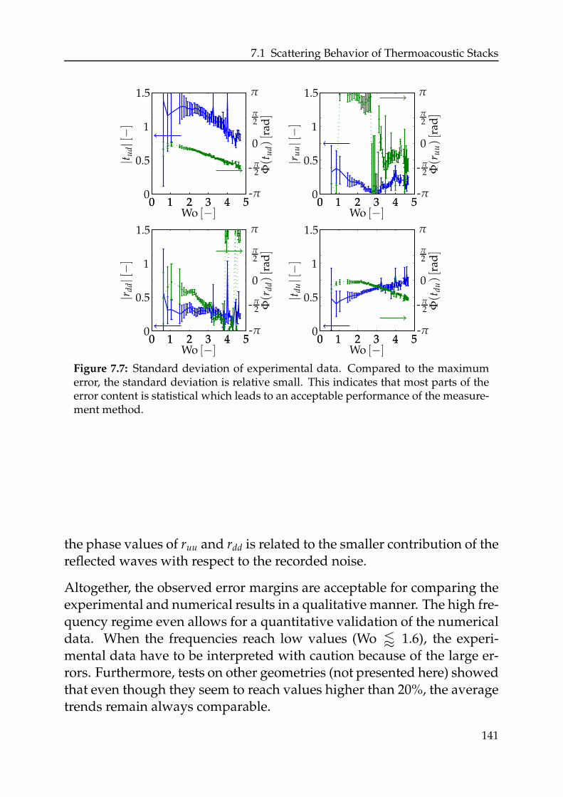
7.1 Scattering Behavior of Thermoacoustic Stacks
0000
00
0000
00
1
1
11
1
1
1
1
11
1
1
2222
2222
3333
3333
4444
4444
5555
5555
0.50.5
0.50.5
1.51.5
1.51.5
Wo [−]Wo [−]
Wo [−]Wo [−]
|t ud|[−]
Φ(t
ud)[r
ad]
|t du|[−]
Φ(t
du)[r
ad]
|r dd|[−]
Φ(r
dd)[r
ad]
|r uu|[−]
Φ(r
uu)[r
ad]
ππ
ππ
π2
π2
π2
π2
00
00
-π2-π
2
-π2-π
2
-π-π
-π-π
Figure 7.7: Standard deviation of experimental data. Compared to the maximumerror, the standard deviation is relative small. This indicates that most parts of theerror content is statistical which leads to an acceptable performance of the measure-ment method.
the phase values of ruu and rdd is related to the smaller contribution of thereflected waves with respect to the recorded noise.
Altogether, the observed error margins are acceptable for comparing theexperimental and numerical results in a qualitative manner. The high fre-quency regime even allows for a quantitative validation of the numericaldata. When the frequencies reach low values (Wo / 1.6), the experi-mental data have to be interpreted with caution because of the large er-rors. Furthermore, tests on other geometries (not presented here) showedthat even though they seem to reach values higher than 20%, the averagetrends remain always comparable.
141
7 Thermoacoustic Interaction in Zero Mean Flow Conditions
7.1.4.4 Minor Sources of Errors
The analysis of the methods applied showed a good reliability of the dataobtained by all the three methods. This comparability is further influ-enced by minor discrepancies. Determining the real contribution of thesedifferences is beyond the scope of this thesis. They are presented as pos-sible sources of error in this section.
The test rig is operating at atmospheric conditions. Consequently, every-day fluctuations in atmospheric conditions, for example humidity takeeffect on the system’s acoustic measurement hardware. Moreover, dueto design reasons, the microphones are not accurately fixed in their po-sitions. The positioning may change slightly during the measurementcampaign. The power supply of the electric heaters is controlled manu-ally. This leads to a power input accuracy lower than 98%. The error ofcontrol thermocouples, which are used to maintain a certain temperaturedistribution, is of the order of 1 K. Although the approximated temper-ature profile (App. B.1) has been validated empirically, the lack of infor-mation about the real multi-dimensional mean temperature field insidethe measurement duct causes a certain uncertainty. The temperature ofthe mains water, which is used to maintain the upstream duct at ambi-ent conditions, changes in time. Deviations of up to 5 K were observedduring the measurement campaigns. Finally, it has to be stated that thecombination of acoustic oscillations and hot temperatures causes a fastmaterial aging of the internal heater and its surrounding components.Especially the ceramic parts are subjected to deterioration at every mea-surement campaign. This leads to a change in geometrical conditions aswell as losses due to imperfect sealing.
The CFD simulation is also subjected to errors. The open source codeOpenFOAM used in the present thesis has rarely been used for aeroa-coustic simulations [117, 118, 191]. There is no publication available treat-ing acoustic propagation under non-isothermal conditions. Thus, its ac-curacy has only been tested to some extent. Kunzer [101] investigateddifferent discretization schemes for incompressible solvers. These weretested in the thesis of Stich. He solved generic compressible test casesby using a PISO looped solver. Altogether, the investigation revealedmuch higher numerical diffusivity than other codes [58]. The use of the
142
7.2 Thermoacoustic Engine Operation Mode
segregated solver is also expected to induce a certain relative time lag ofpressure, velocity and temperature oscillation. Also, the computation ofthe thermophysical properties causes small discrepancies to experimen-tal and one-dimensional data. Finally, although the temperature profileswere sufficiently resolved, the investigation of higher Pe cases is lim-ited by the mesh resolution. In this case, local refinement will not onlycause an increasing number of degrees of freedom, but also a necessity ofreducing the time step to maintain an acoustic CFL-number lower thanunity.
The one-dimensional numerical tool is expected to be the least error-prone. The usage of a fine discretization and a higher-order integrationscheme only induces small errors. The highest numerical errors occurfor low frequencies [72]. The computation of the matrix coefficients of A
(Eq. (4.63)) for every step causes an error accumulation, which leads tounphysical results. A preliminary computation of these components incombination with interpolation at the current position circumvents thisproblem.
7.2 Thermoacoustic Engine Operation Mode
Two states of the TA engine setup facilitate a validation of the scatteringmatrices obtained. The cycle increment [75, 192] in the linear onset ofthe engine is comparable to the data obtained from the eigenfrequencyanalysis of a network model. The limit cycle delivers qualitative infor-mation about the ratio of losses, higher-order modes and damping insidethe system. Moreover, the reconstructed mode shape of the first eigen-mode allows a comparison of the reference plane data to the predictedvalues obtained by numerical and experimental techniques. All the time-dependent data presented in this chapter refer to the signal depicted inFigure 7.8. The measurement data for this plot are obtained for one TAengine operation point (Lw = 1.1 m). An average temperature differ-ence of approximately 100 K was preset over the stack by controlling thepower supply of the inner heater.
The onset was produced by dismounting a plug at a central position inthe cold channel, such that all instabilities break down. As soon as all
143
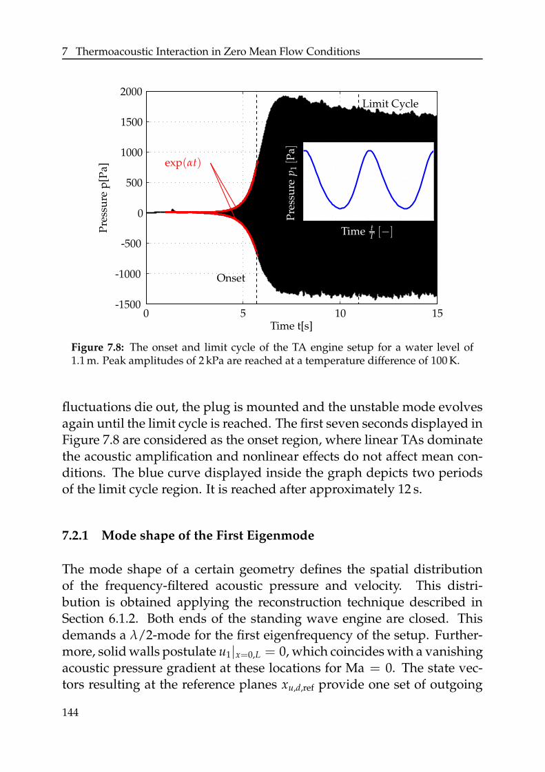
7 Thermoacoustic Interaction in Zero Mean Flow Conditions
0
0 5 10 15
500
1000
1500
2000
-500
-1000
-1500
Time t[s]
Pre
ssu
rep
[Pa]
Time tT [−]
Pre
ssu
rep
1[P
a]
Limit Cycle
Onset
exp(αt)
Figure 7.8: The onset and limit cycle of the TA engine setup for a water level of1.1 m. Peak amplitudes of 2 kPa are reached at a temperature difference of 100 K.
fluctuations die out, the plug is mounted and the unstable mode evolvesagain until the limit cycle is reached. The first seven seconds displayed inFigure 7.8 are considered as the onset region, where linear TAs dominatethe acoustic amplification and nonlinear effects do not affect mean con-ditions. The blue curve displayed inside the graph depicts two periodsof the limit cycle region. It is reached after approximately 12 s.
7.2.1 Mode shape of the First Eigenmode
The mode shape of a certain geometry defines the spatial distributionof the frequency-filtered acoustic pressure and velocity. This distri-bution is obtained applying the reconstruction technique described inSection 6.1.2. Both ends of the standing wave engine are closed. Thisdemands a λ/2-mode for the first eigenfrequency of the setup. Further-more, solid walls postulate u1|x=0,L = 0, which coincides with a vanishingacoustic pressure gradient at these locations for Ma = 0. The state vec-tors resulting at the reference planes xu,d,ref provide one set of outgoing
144
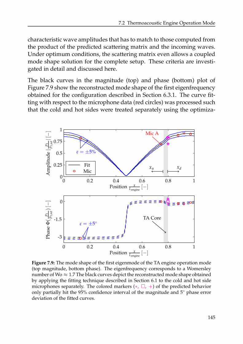
7.2 Thermoacoustic Engine Operation Mode
characteristic wave amplitudes that has to match to those computed fromthe product of the predicted scattering matrix and the incoming waves.Under optimum conditions, the scattering matrix even allows a coupledmode shape solution for the complete setup. These criteria are investi-gated in detail and discussed here.
The black curves in the magnitude (top) and phase (bottom) plot ofFigure 7.9 show the reconstructed mode shape of the first eigenfrequencyobtained for the configuration described in Section 6.3.1. The curve fit-ting with respect to the microphone data (red circles) was processed suchthat the cold and hot sides were treated separately using the optimiza-
0
0
00
1
1
1
0.25
0.75
-1.5
-3
0.2
0.2
0.4
0.4
0.5
0.6
0.6
0.8
0.8
Position xLengine
[−]
Position xLengine
[−]
Am
pli
tud
e|
p1
p1,
ref|[−]
Ph
ase
Φ(
p1
p1,
ref)[−
]
FitMic
ε = ±5%
ε = ±5TA Core
Mic A
xu xd
Figure 7.9: The mode shape of the first eigenmode of the TA engine operation mode(top magnitude, bottom phase). The eigenfrequency corresponds to a Womersleynumber of Wo ≈ 1.7 The black curves depict the reconstructed mode shape obtainedby applying the fitting technique described in Section 6.1 to the cold and hot sidemicrophones separately. The colored markers (∗, , +) of the predicted behavioronly partially hit the 95% confidence interval of the magnitude and 5 phase errordeviation of the fitted curves.
145
7 Thermoacoustic Interaction in Zero Mean Flow Conditions
tion method described in Section 6.1.1. The curves in the TA core regionare linear interpolations and no computed intermediate values. The bluecurves describe the confidence intervals of 95% for the magnitude curveand a ±5 discrepancy to the dashed phase plot. All five microphonemeasurements (red circles) are within this range. These microphones arenot located near the pressure antinode of the profile. The measured pres-sure data has high amplitude values and hence, the reconstructed modeshape is not affected by the standing wave pattern. Due to the use oftwo microphones at the cold side, the fitting problem (Eq. (6.4)) with twocomplex-valued degrees of freedom is not overdetermined. Thus, thispart of the curves coincides with the measurement values. The micro-phones are known to predict the most accurate results for ambient condi-tions, which also provide the most reliable mean quantity data. Detailedtests revealed that these measurements can lead to errors of 2 − 3%. Thehot curve fit was obtained using a measurement based linear temperaturedistribution according to
T0(x) = 400 K − 50 Kxd
Ld(7.4)
and a temperature stepping of 1 K for each discrete change in mean tem-perature. Due to the increased number of microphones, the problem be-comes overdetermined. The fitting to the less accurate mean temperaturedata in the downstream (0.8 < x/Lengine < 1) lead to clearly visible devi-ations.
As both ends of the engine are completely sealed, a typical λ/2 modeshape is expected with both ends having a zero gradient in |p1|. More-over, the pressure at these locations is expected to oscillate with a phasedifference of π. The upstream pressure gradient at x = 0 almost reacheszero. This indicates that: a) the fit is in good accordance to the measure-ment data in the frequency range below the cut-on frequency of transver-sal modes and b) the water column in the duct causes a hard wall reflec-tion coefficient of
F
G
∣∣∣∣
x=0
≈ 1. (7.5)
In contrast to this good match of fit and estimated pressure profile, thedownstream tangent of |p1(Lengine)| is slightly negative. Combined withthe phase shift of these positions of more than π, this indicates a certain
146
7.2 Thermoacoustic Engine Operation Mode
error in the predicted fit. This discrepancy may originate from differentreasons: i) the estimated temperature distribution is not accurate enough.ii) Although the pressure sensors are water cooled, the heating causes acertain impact on the output data. iii) A bad preparation of the micro-phone leads to deviations from the calibrated state.
The quality of the three prediction tools is compared in terms of the ma-genta colored markers in Figure 7.9. They denote the pressure valuespredicted by computing the hot downstream value from the upstreamreference state. For this purpose, the scattering matrix values obtainedusing the MMM (∗), the CFD/SI method () and the one-dimensionalprediction tool (+) for the first eigenfrequency Wo ≈ 1.65 are extracted.Next, applying Equations (3.24) and (3.26) these values are transformedinto transfer matrix data in pu notation. Finally multiplying the acousticstate vector of the upstream plane by these matrices yields the predictedp1 values at the downstream end of the stack. The experimental results(∗) show the strongest deviation. The measurement error at the operatingpoint of Wo ≈ 1.65 is too large to produce reasonable results. The pre-dicted pressure amplitudes of the CFD data () match to the predictedshape on the hot left side. This is not valid for the phase value. It devi-ates half as much as the experimental data, but the confidence intervalis not captured. This deviation is related to the different cross-sectionalshapes of the pores. As shown later (Fig. 7.12), the impact of this param-eter causes the largest deviations in this region. Using the right cross-sectional shape values obtained from the one-dimensional model IMP
(+) leads to a match within the confidence intervals. Here and in the nextsection, the scattering matrix was obtained for quadratic pore shapes ofequal hydraulic radius R. Apart from the validation of experimental re-sults in Section 7.1.3, this adaption is presented only in this section.
7.2.2 Thermoacoustic Onset
The pressure data displayed in Figure 7.8 are recorded in the cold ductat the position of microphone A, which is denoted “Mic A” in Figure 7.9.The reconstructed mode shape leads to a factor of ≈ 1.3 between thepressure value at the downstream antinode and the measured value atlocation A. However, as the cycle increment in the linear acoustic regime
147
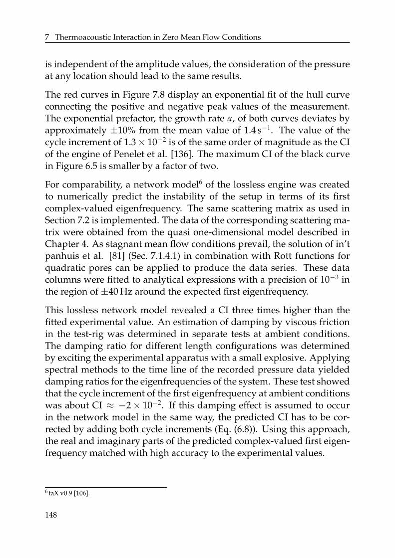
7 Thermoacoustic Interaction in Zero Mean Flow Conditions
is independent of the amplitude values, the consideration of the pressureat any location should lead to the same results.
The red curves in Figure 7.8 display an exponential fit of the hull curveconnecting the positive and negative peak values of the measurement.The exponential prefactor, the growth rate α, of both curves deviates byapproximately ±10% from the mean value of 1.4 s−1. The value of thecycle increment of 1.3 × 10⁻² is of the same order of magnitude as the CIof the engine of Penelet et al. [136]. The maximum CI of the black curvein Figure 6.5 is smaller by a factor of two.
For comparability, a network model6 of the lossless engine was createdto numerically predict the instability of the setup in terms of its firstcomplex-valued eigenfrequency. The same scattering matrix as used inSection 7.2 is implemented. The data of the corresponding scattering ma-trix were obtained from the quasi one-dimensional model described inChapter 4. As stagnant mean flow conditions prevail, the solution of in’tpanhuis et al. [81] (Sec. 7.1.4.1) in combination with Rott functions forquadratic pores can be applied to produce the data series. These datacolumns were fitted to analytical expressions with a precision of 10−3 inthe region of ±40 Hz around the expected first eigenfrequency.
This lossless network model revealed a CI three times higher than thefitted experimental value. An estimation of damping by viscous frictionin the test-rig was determined in separate tests at ambient conditions.The damping ratio for different length configurations was determinedby exciting the experimental apparatus with a small explosive. Applyingspectral methods to the time line of the recorded pressure data yieldeddamping ratios for the eigenfrequencies of the system. These test showedthat the cycle increment of the first eigenfrequency at ambient conditionswas about CI ≈ −2 × 10⁻². If this damping effect is assumed to occurin the network model in the same way, the predicted CI has to be cor-rected by adding both cycle increments (Eq. (6.8)). Using this approach,the real and imaginary parts of the predicted complex-valued first eigen-frequency matched with high accuracy to the experimental values.
6 taX v0.9 [106].
148
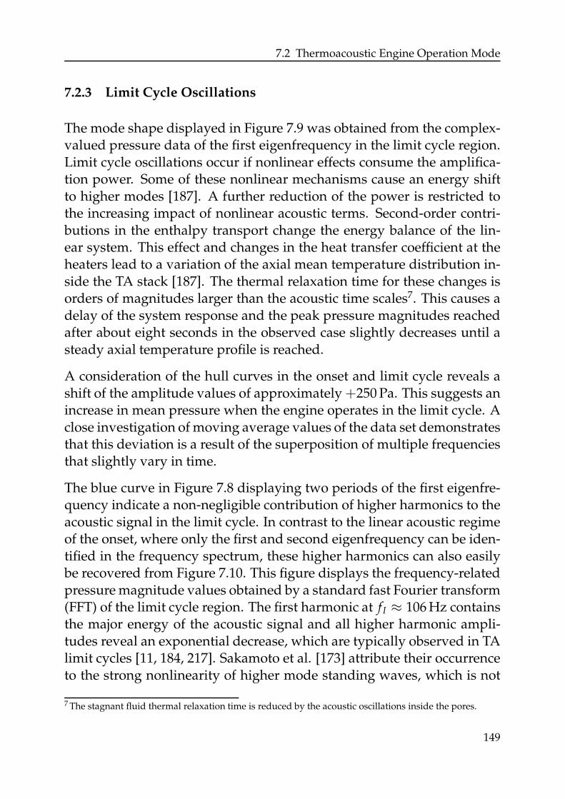
7.2 Thermoacoustic Engine Operation Mode
7.2.3 Limit Cycle Oscillations
The mode shape displayed in Figure 7.9 was obtained from the complex-valued pressure data of the first eigenfrequency in the limit cycle region.Limit cycle oscillations occur if nonlinear effects consume the amplifica-tion power. Some of these nonlinear mechanisms cause an energy shiftto higher modes [187]. A further reduction of the power is restricted tothe increasing impact of nonlinear acoustic terms. Second-order contri-butions in the enthalpy transport change the energy balance of the lin-ear system. This effect and changes in the heat transfer coefficient at theheaters lead to a variation of the axial mean temperature distribution in-side the TA stack [187]. The thermal relaxation time for these changes isorders of magnitudes larger than the acoustic time scales7. This causes adelay of the system response and the peak pressure magnitudes reachedafter about eight seconds in the observed case slightly decreases until asteady axial temperature profile is reached.
A consideration of the hull curves in the onset and limit cycle reveals ashift of the amplitude values of approximately +250 Pa. This suggests anincrease in mean pressure when the engine operates in the limit cycle. Aclose investigation of moving average values of the data set demonstratesthat this deviation is a result of the superposition of multiple frequenciesthat slightly vary in time.
The blue curve in Figure 7.8 displaying two periods of the first eigenfre-quency indicate a non-negligible contribution of higher harmonics to theacoustic signal in the limit cycle. In contrast to the linear acoustic regimeof the onset, where only the first and second eigenfrequency can be iden-tified in the frequency spectrum, these higher harmonics can also easilybe recovered from Figure 7.10. This figure displays the frequency-relatedpressure magnitude values obtained by a standard fast Fourier transform(FFT) of the limit cycle region. The first harmonic at f I ≈ 106 Hz containsthe major energy of the acoustic signal and all higher harmonic ampli-tudes reveal an exponential decrease, which are typically observed in TAlimit cycles [11, 184, 217]. Sakamoto et al. [173] attribute their occurrenceto the strong nonlinearity of higher mode standing waves, which is not
7 The stagnant fluid thermal relaxation time is reduced by the acoustic oscillations inside the pores.
149
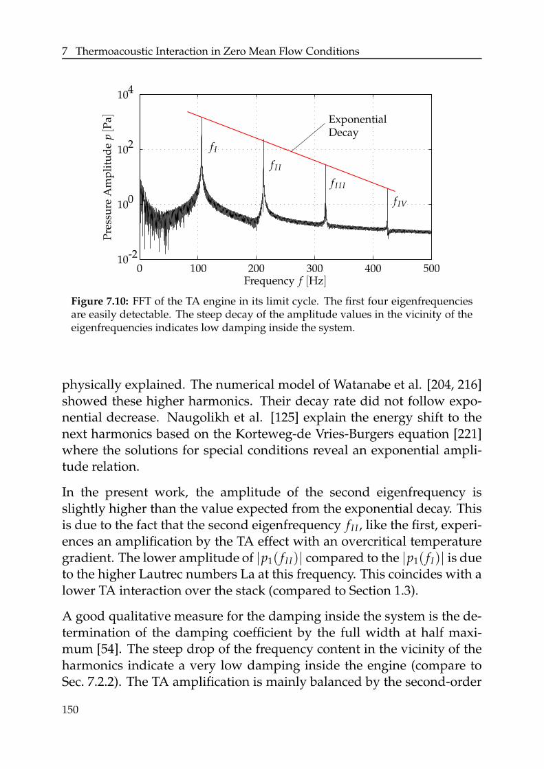
7 Thermoacoustic Interaction in Zero Mean Flow Conditions
0
0
2
410
10
10
10-2
100 200 300 400 500Frequency f [Hz]
Pre
ssu
reA
mp
litu
de
p[P
a]
ExponentialDecay
f IV
f I I I
f I I
f I
Figure 7.10: FFT of the TA engine in its limit cycle. The first four eigenfrequenciesare easily detectable. The steep decay of the amplitude values in the vicinity of theeigenfrequencies indicates low damping inside the system.
physically explained. The numerical model of Watanabe et al. [204, 216]showed these higher harmonics. Their decay rate did not follow expo-nential decrease. Naugolikh et al. [125] explain the energy shift to thenext harmonics based on the Korteweg-de Vries-Burgers equation [221]where the solutions for special conditions reveal an exponential ampli-tude relation.
In the present work, the amplitude of the second eigenfrequency isslightly higher than the value expected from the exponential decay. Thisis due to the fact that the second eigenfrequency f I I , like the first, experi-ences an amplification by the TA effect with an overcritical temperaturegradient. The lower amplitude of |p1( f I I)| compared to the |p1( f I)| is dueto the higher Lautrec numbers La at this frequency. This coincides with alower TA interaction over the stack (compared to Section 1.3).
A good qualitative measure for the damping inside the system is the de-termination of the damping coefficient by the full width at half maxi-mum [54]. The steep drop of the frequency content in the vicinity of theharmonics indicate a very low damping inside the engine (compare toSec. 7.2.2). The TA amplification is mainly balanced by the second-order
150
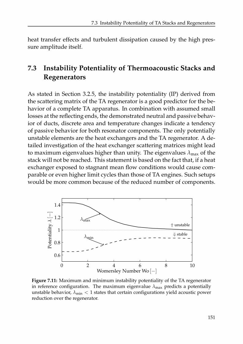
7.3 Instability Potentiality of TA Stacks and Regenerators
heat transfer effects and turbulent dissipation caused by the high pres-sure amplitude itself.
7.3 Instability Potentiality of Thermoacoustic Stacks and
Regenerators
As stated in Section 3.2.5, the instability potentiality (IP) derived fromthe scattering matrix of the TA regenerator is a good predictor for the be-havior of a complete TA apparatus. In combination with assumed smalllosses at the reflecting ends, the demonstrated neutral and passive behav-ior of ducts, discrete area and temperature changes indicate a tendencyof passive behavior for both resonator components. The only potentiallyunstable elements are the heat exchangers and the TA regenerator. A de-tailed investigation of the heat exchanger scattering matrices might leadto maximum eigenvalues higher than unity. The eigenvalues λmax of thestack will not be reached. This statement is based on the fact that, if a heatexchanger exposed to stagnant mean flow conditions would cause com-parable or even higher limit cycles than those of TA engines. Such setupswould be more common because of the reduced number of components.
0
1
2 4 6 8 10
0.6
0.8
1.2
1.4
Womersley Number Wo [−]
Po
ten
tial
ity
λ[−
]
⇑ unstable
⇓ stableλmin
λmax
Figure 7.11: Maximum and minimum instability potentiality of the TA regeneratorin reference configuration. The maximum eigenvalue λmax predicts a potentiallyunstable behavior, λmin < 1 states that certain configurations yield acoustic powerreduction over the regenerator.
151
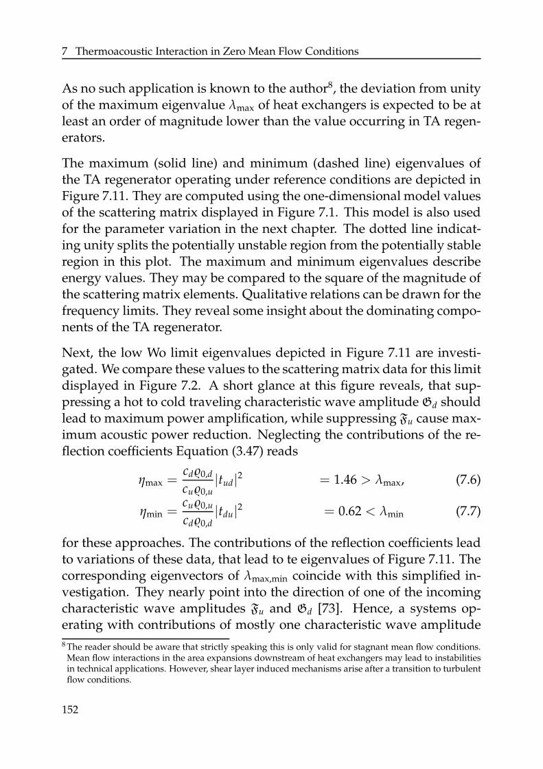
7 Thermoacoustic Interaction in Zero Mean Flow Conditions
As no such application is known to the author8, the deviation from unityof the maximum eigenvalue λmax of heat exchangers is expected to be atleast an order of magnitude lower than the value occurring in TA regen-erators.
The maximum (solid line) and minimum (dashed line) eigenvalues ofthe TA regenerator operating under reference conditions are depicted inFigure 7.11. They are computed using the one-dimensional model valuesof the scattering matrix displayed in Figure 7.1. This model is also usedfor the parameter variation in the next chapter. The dotted line indicat-ing unity splits the potentially unstable region from the potentially stableregion in this plot. The maximum and minimum eigenvalues describeenergy values. They may be compared to the square of the magnitude ofthe scattering matrix elements. Qualitative relations can be drawn for thefrequency limits. They reveal some insight about the dominating compo-nents of the TA regenerator.
Next, the low Wo limit eigenvalues depicted in Figure 7.11 are investi-gated. We compare these values to the scattering matrix data for this limitdisplayed in Figure 7.2. A short glance at this figure reveals, that sup-pressing a hot to cold traveling characteristic wave amplitude Gd shouldlead to maximum power amplification, while suppressing Fu cause max-imum acoustic power reduction. Neglecting the contributions of the re-flection coefficients Equation (3.47) reads
ηmax =cd0,d
cu0,u|tud|2 = 1.46 > λmax, (7.6)
ηmin =cu0,u
cd0,d|tdu|2 = 0.62 < λmin (7.7)
for these approaches. The contributions of the reflection coefficients leadto variations of these data, that lead to te eigenvalues of Figure 7.11. Thecorresponding eigenvectors of λmax,min coincide with this simplified in-vestigation. They nearly point into the direction of one of the incomingcharacteristic wave amplitudes Fu and Gd [73]. Hence, a systems op-erating with contributions of mostly one characteristic wave amplitude
8 The reader should be aware that strictly speaking this is only valid for stagnant mean flow conditions.Mean flow interactions in the area expansions downstream of heat exchangers may lead to instabilitiesin technical applications. However, shear layer induced mechanisms arise after a transition to turbulentflow conditions.
152
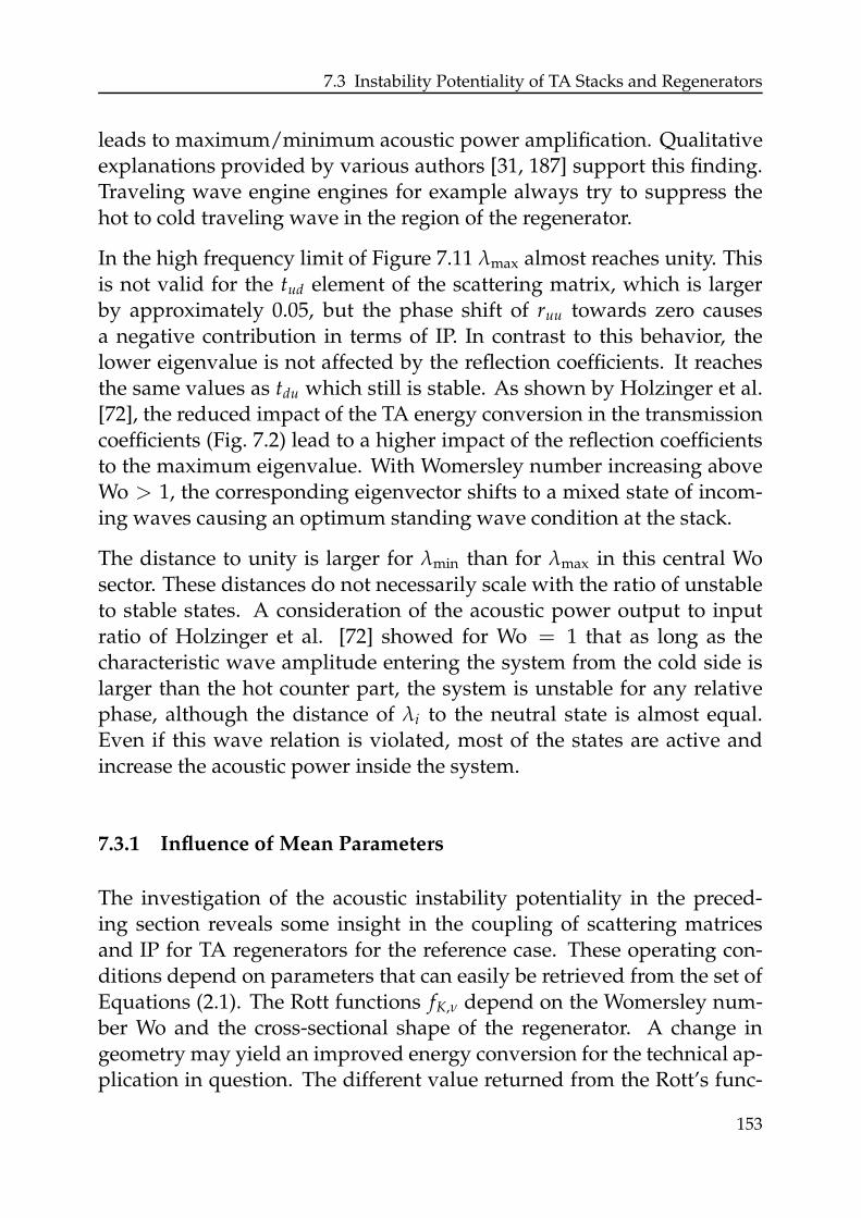
7.3 Instability Potentiality of TA Stacks and Regenerators
leads to maximum/minimum acoustic power amplification. Qualitativeexplanations provided by various authors [31, 187] support this finding.Traveling wave engine engines for example always try to suppress thehot to cold traveling wave in the region of the regenerator.
In the high frequency limit of Figure 7.11 λmax almost reaches unity. Thisis not valid for the tud element of the scattering matrix, which is largerby approximately 0.05, but the phase shift of ruu towards zero causesa negative contribution in terms of IP. In contrast to this behavior, thelower eigenvalue is not affected by the reflection coefficients. It reachesthe same values as tdu which still is stable. As shown by Holzinger et al.[72], the reduced impact of the TA energy conversion in the transmissioncoefficients (Fig. 7.2) lead to a higher impact of the reflection coefficientsto the maximum eigenvalue. With Womersley number increasing aboveWo > 1, the corresponding eigenvector shifts to a mixed state of incom-ing waves causing an optimum standing wave condition at the stack.
The distance to unity is larger for λmin than for λmax in this central Wosector. These distances do not necessarily scale with the ratio of unstableto stable states. A consideration of the acoustic power output to inputratio of Holzinger et al. [72] showed for Wo = 1 that as long as thecharacteristic wave amplitude entering the system from the cold side islarger than the hot counter part, the system is unstable for any relativephase, although the distance of λi to the neutral state is almost equal.Even if this wave relation is violated, most of the states are active andincrease the acoustic power inside the system.
7.3.1 Influence of Mean Parameters
The investigation of the acoustic instability potentiality in the preced-ing section reveals some insight in the coupling of scattering matricesand IP for TA regenerators for the reference case. These operating con-ditions depend on parameters that can easily be retrieved from the set ofEquations (2.1). The Rott functions fK,ν depend on the Womersley num-ber Wo and the cross-sectional shape of the regenerator. A change ingeometry may yield an improved energy conversion for the technical ap-plication in question. The different value returned from the Rott’s func-
153
7 Thermoacoustic Interaction in Zero Mean Flow Conditions
tions fK,ν for one frequency is related to their scaling with Pr. The use ofdifferent fluids may significantly change the IP of the problem. Viscousdissipation and thermal diffusion both also scale with mean pressure p0.A pressurization leads to changes in the scattering behavior. Finally, theTA amplification term scales with mean temperature T0. The investiga-tion of different temperature differences over the stack should influencethe IP of the TA regenerator. For yielding a certain insight into the impactof those parameters, they are varied in the next sections. Combinationsof parameter variations, which might lead to optimum conditions, arebeyond the scope of this work and not considered here.
7.3.1.1 Influence of the Cross-Sectional Pore Shape
0
1
2 4 6 8 100.5
1.5
Womersley Number Wo [−]
Po
ten
tial
ity
λ[−
]
©
≡
Figure 7.12: Maximum and minimum IP for different cross-sectional shapes in thereference configuration. In the region of 1 . Wo . 4, where Rott’s functions deviatemost [187], the maximum potentiality varies. The minimum potentialities of thecircular (©) and quadratic () shaped pores are higher than for slab pores.
The viscous Rott’s functions describing slab stacked (≡), quadratic ()and circular shaped pores (©) are defined by [187]
fν,≡ =2 tanh
(1+i
2 Wo)
(1 + i)Wo, (7.8a)
fν, = 1 − 64
π4 ∑m,nodd
1
m2n2(
1 − 2i[
π4Wo
)2(m2 + n2)
] , (7.8b)
154
7.3 Instability Potentiality of TA Stacks and Regenerators
fν,© =2J1 [(i − 1)Wo]
(i − 1)Wo J [(i − 1)Wo]. (7.8c)
If the thermal penetration depth δK is considered, the Womersley num-ber Wo is replaced by the Lautrec number La. As these dimensionlessnumbers scale with the square root of the Prandtl number Pr (Tab. 4.1),their ratio is fixed by the chosen operating fluid. Especially the real val-ues of these functions deviate for 1 . Wo . 5. Their impact on the IP ismainly restricted to this region.
Figure 7.12 depicts λmin,max for these three cross-section geometries. Thehigh and low frequency values of the profiles of both quantities stay un-affected. Circular and quadratic pores lead to almost equal eigenvaluesexcept for a small intermediate Wo region.
The peak IPs are reached by circular pores for Wo ≈ 1.5. The radialsymmetry of the boundary layers improves the energy conversion withrespect to the axial symmetric shapes occurring in the other profiles. Thelower performance of the slab pores profile at the region of maximum IPis due to the lower change in phase for f≡. The smoother phase changeof the parallel plate geometry coincides with larger magnitude values ofthe Rott function. Thus, while the circular pores are favorable for low Wo,slab geometries lead to a better performance for applications operating atWo > 2. The higher amplitude values of f≡ also increase the impact inA12 and A21 of the set of transport Equation (2.1), which strongly con-tribute to λmin. The higher damping causes lower minimum eigenvaluesover the entire Womersley number range.
7.3.1.2 Material Properties of the Fluid
The ratio of viscous diffusion to thermal conductivity is a characteris-tic quantity for many energy conversion processes. Here, the Prandtlnumber Pr is not just a scaling factor for the TA interaction term A22 ofEquation (2.1a). It also determines the value of the thermal Rott func-tion fK for a given Womersley number Wo and thus has an impact on thefull system of Equations (2.1). In Figure 7.13 this impact is investigatedin terms of a change in the heat conduction K of air. The standard case(black) of Pr ≈ 0.7 is depicted for orientation purposes. This value is
155
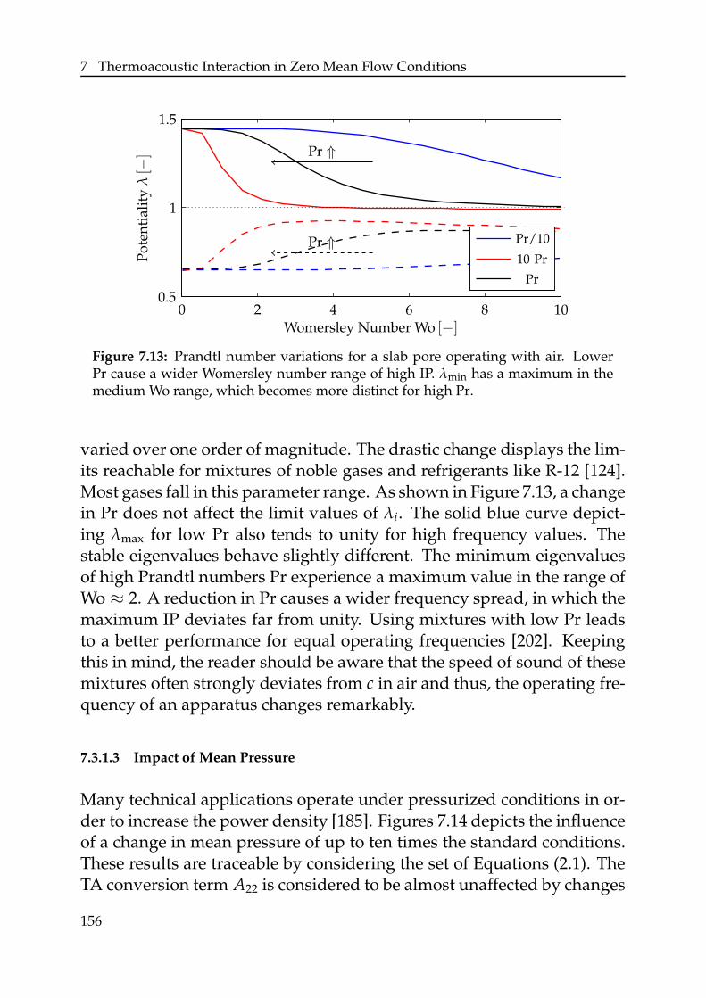
7 Thermoacoustic Interaction in Zero Mean Flow Conditions
0
1
2 4 6 8 100.5
1.5
Womersley Number Wo [−]
Po
ten
tial
ity
λ[−
]
Pr/10
10 Pr
Pr
Pr ⇑
Pr ⇑
Figure 7.13: Prandtl number variations for a slab pore operating with air. LowerPr cause a wider Womersley number range of high IP. λmin has a maximum in themedium Wo range, which becomes more distinct for high Pr.
varied over one order of magnitude. The drastic change displays the lim-its reachable for mixtures of noble gases and refrigerants like R-12 [124].Most gases fall in this parameter range. As shown in Figure 7.13, a changein Pr does not affect the limit values of λi. The solid blue curve depict-ing λmax for low Pr also tends to unity for high frequency values. Thestable eigenvalues behave slightly different. The minimum eigenvaluesof high Prandtl numbers Pr experience a maximum value in the range ofWo ≈ 2. A reduction in Pr causes a wider frequency spread, in which themaximum IP deviates far from unity. Using mixtures with low Pr leadsto a better performance for equal operating frequencies [202]. Keepingthis in mind, the reader should be aware that the speed of sound of thesemixtures often strongly deviates from c in air and thus, the operating fre-quency of an apparatus changes remarkably.
7.3.1.3 Impact of Mean Pressure
Many technical applications operate under pressurized conditions in or-der to increase the power density [185]. Figures 7.14 depicts the influenceof a change in mean pressure of up to ten times the standard conditions.These results are traceable by considering the set of Equations (2.1). TheTA conversion term A22 is considered to be almost unaffected by changes
156
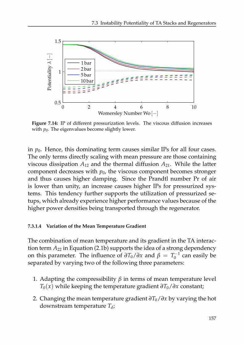
7.3 Instability Potentiality of TA Stacks and Regenerators
0
1
2 4 6 8 100.5
1.5
Womersley Number Wo [−]
Po
ten
tial
ity
λ[−
]
1 bar2 bar5 bar10 bar
Figure 7.14: IP of different pressurization levels. The viscous diffusion increaseswith p0. The eigenvalues become slightly lower.
in p0. Hence, this dominating term causes similar IPs for all four cases.The only terms directly scaling with mean pressure are those containingviscous dissipation A12 and the thermal diffusion A21. While the lattercomponent decreases with p0, the viscous component becomes strongerand thus causes higher damping. Since the Prandtl number Pr of airis lower than unity, an increase causes higher IPs for pressurized sys-tems. This tendency further supports the utilization of pressurized se-tups, which already experience higher performance values because of thehigher power densities being transported through the regenerator.
7.3.1.4 Variation of the Mean Temperature Gradient
The combination of mean temperature and its gradient in the TA interac-tion term A22 in Equation (2.1b) supports the idea of a strong dependencyon this parameter. The influence of ∂T0/∂x and β = T−1
0 can easily beseparated by varying two of the following three parameters:
1. Adapting the compressibility β in terms of mean temperature levelT0(x) while keeping the temperature gradient ∂T0/∂x constant;
2. Changing the mean temperature gradient ∂T0/∂x by varying the hotdownstream temperature Td;
157
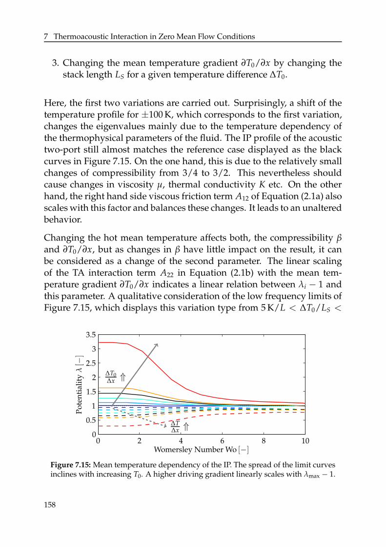
7 Thermoacoustic Interaction in Zero Mean Flow Conditions
3. Changing the mean temperature gradient ∂T0/∂x by changing thestack length LS for a given temperature difference ∆T0.
Here, the first two variations are carried out. Surprisingly, a shift of thetemperature profile for ±100 K, which corresponds to the first variation,changes the eigenvalues mainly due to the temperature dependency ofthe thermophysical parameters of the fluid. The IP profile of the acoustictwo-port still almost matches the reference case displayed as the blackcurves in Figure 7.15. On the one hand, this is due to the relatively smallchanges of compressibility from 3/4 to 3/2. This nevertheless shouldcause changes in viscosity µ, thermal conductivity K etc. On the otherhand, the right hand side viscous friction term A12 of Equation (2.1a) alsoscales with this factor and balances these changes. It leads to an unalteredbehavior.
Changing the hot mean temperature affects both, the compressibility βand ∂T0/∂x, but as changes in β have little impact on the result, it canbe considered as a change of the second parameter. The linear scalingof the TA interaction term A22 in Equation (2.1b) with the mean tem-perature gradient ∂T0/∂x indicates a linear relation between λi − 1 andthis parameter. A qualitative consideration of the low frequency limits ofFigure 7.15, which displays this variation type from 5 K/L < ∆T0/LS <
00
1
2
2
3
4 6 8 10
2.5
3.5
0.5
1.5
Womersley Number Wo [−]
Po
ten
tial
ity
λ[−
]
∆T0∆x
⇑
∆T∆x
⇑
Figure 7.15: Mean temperature dependency of the IP. The spread of the limit curvesinclines with increasing T0. A higher driving gradient linearly scales with λmax − 1.
158
7.3 Instability Potentiality of TA Stacks and Regenerators
300 K/L, yields a linear relation between λmax − 1 and the temperaturegradient. The blue colored curves denote a temperature gradient of 5 K(dark blue), 10 K and 50 K (light blue) per stack length L. The distancebetween the orange colored 200 K/L and the reference case depicted inblack is as large as the distance between the former curve and the max-imum IP of 300 K/L. No saturation limit is reached for the investigatedtemperature gradients. It is expected that the maximum acoustic poweroutput ratio always scales linearly with an increase in temperature dif-ference. The power output is further affected by diffusion. Such effectsare taken into account by the D-TC-D model treated in Section 7.1.2.Figure 3.4 shows that if dissipative effects are taken into account in theducts, both eigenvalues D-TC-D decrease from unity for higher Wom-ersley numbers Wo. Hence, considering Wo > 0, the offset of the linearscaling with the temperature gradient changes. The offset follows thedecaying lines of the eigenvalues λD−TC−D,max of the simplified model.The linear scaling factor is computed from λmax − λD-TC-D,max for varyingWomersley numbers and temperature gradients.
The variation of the regenerator length for constant temperatures at bothends was also investigated for reasons of completeness. However, thechange in the results verified that the impact of the change in β is negli-gible compared to a variation of the temperature gradient.
The temperature gradient affects the TA interaction locally. One mightexpect that a change in the temperature profile T0(x) caused by meanflow u0 or higher-order effects could lead to other IPs than the onesshown here. For implicit modeling (IMP), mean flow changes only re-sult in an adaption of T0(x). However, due to the linear scaling of therelevant term, the overall impact of different mean temperature profilesT0(x) neither affects the scattering matrices nor the IP of TA regenerators.Impacts of mean flow, which are captured by the other demonstratedmodels, are investigated in the next chapter. As the observed influencesdo not change the nature of the scattering matrices and low Ma affectthe IP computation by 1 ± Ma−1, their impact on IP is not considered forthese cases.
159

7 Thermoacoustic Interaction in Zero Mean Flow Conditions
160
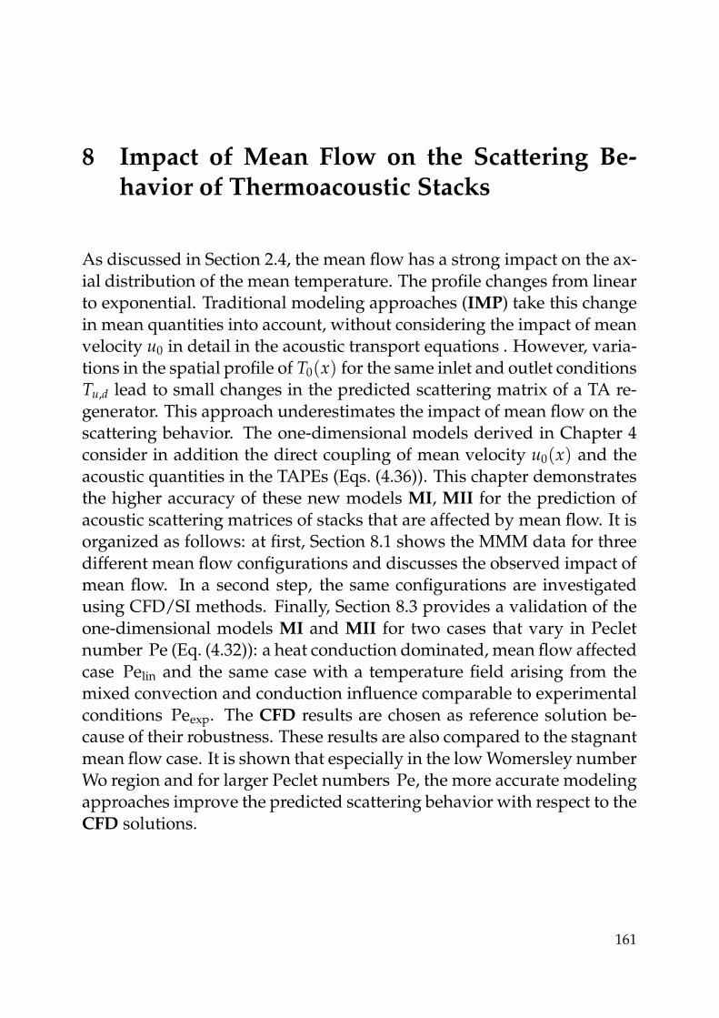
8 Impact of Mean Flow on the Scattering Be-havior of Thermoacoustic Stacks
As discussed in Section 2.4, the mean flow has a strong impact on the ax-ial distribution of the mean temperature. The profile changes from linearto exponential. Traditional modeling approaches (IMP) take this changein mean quantities into account, without considering the impact of meanvelocity u0 in detail in the acoustic transport equations . However, varia-tions in the spatial profile of T0(x) for the same inlet and outlet conditionsTu,d lead to small changes in the predicted scattering matrix of a TA re-generator. This approach underestimates the impact of mean flow on thescattering behavior. The one-dimensional models derived in Chapter 4consider in addition the direct coupling of mean velocity u0(x) and theacoustic quantities in the TAPEs (Eqs. (4.36)). This chapter demonstratesthe higher accuracy of these new models MI, MII for the prediction ofacoustic scattering matrices of stacks that are affected by mean flow. It isorganized as follows: at first, Section 8.1 shows the MMM data for threedifferent mean flow configurations and discusses the observed impact ofmean flow. In a second step, the same configurations are investigatedusing CFD/SI methods. Finally, Section 8.3 provides a validation of theone-dimensional models MI and MII for two cases that vary in Pecletnumber Pe (Eq. (4.32)): a heat conduction dominated, mean flow affectedcase Pelin and the same case with a temperature field arising from themixed convection and conduction influence comparable to experimentalconditions Peexp. The CFD results are chosen as reference solution be-cause of their robustness. These results are also compared to the stagnantmean flow case. It is shown that especially in the low Womersley numberWo region and for larger Peclet numbers Pe, the more accurate modelingapproaches improve the predicted scattering behavior with respect to theCFD solutions.
161
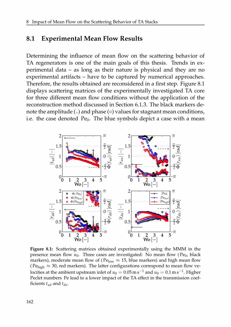
8 Impact of Mean Flow on the Scattering Behavior of TA Stacks
8.1 Experimental Mean Flow Results
Determining the influence of mean flow on the scattering behavior ofTA regenerators is one of the main goals of this thesis. Trends in ex-perimental data – as long as their nature is physical and they are noexperimental artifacts – have to be captured by numerical approaches.Therefore, the results obtained are reconsidered in a first step. Figure 8.1displays scattering matrices of the experimentally investigated TA corefor three different mean flow conditions without the application of thereconstruction method discussed in Section 6.1.3. The black markers de-note the amplitude (+) and phase () values for stagnant mean conditions,i.e. the case denoted Pe0. The blue symbols depict a case with a mean
00
00
00
00
00
00
11
11
1
1
1
1
1
1
1
1
22
22
2
2
2
2
2
2
2
2
33
33
33
33
44
44
44
44
55
55
55
55
0.50.5
0.50.5
1.51.5
1.51.5
Wo [−]Wo [−]
Wo [−]Wo [−]
Wo [−]Wo [−]
Wo [−]Wo [−]
|t ud|[−]
Φ(t
ud)[r
ad]
|t du|[−]
Φ(t
du)[r
ad]
|r dd|[−]
Φ(r
dd)[r
ad]
|r uu|[−]
Φ(r
uu)[r
ad]
ππ
ππ
π2
π2
π2
π2
00
00
-π2-π
2
-π2-π
2
-π-π
-π-π
|Pe0|Φ( Pe0)|Pelow|Φ(Pelow)|Pehigh|Φ(Pehigh)
Figure 8.1: Scattering matrices obtained experimentally using the MMM in thepresence mean flow u0. Three cases are investigated: No mean flow ( Pe0, blackmarkers), moderate mean flow of ( Pelow ≈ 15, blue markers) and high mean flow( Pehigh ≈ 30, red markers). The latter configurations correspond to mean flow ve-
locities at the ambient upstream inlet of u0 = 0.05 m s−1 and u0 = 0.1 m s−1. HigherPeclet numbers Pe lead to a lower impact of the TA effect in the transmission coef-ficients tud and tdu.
162
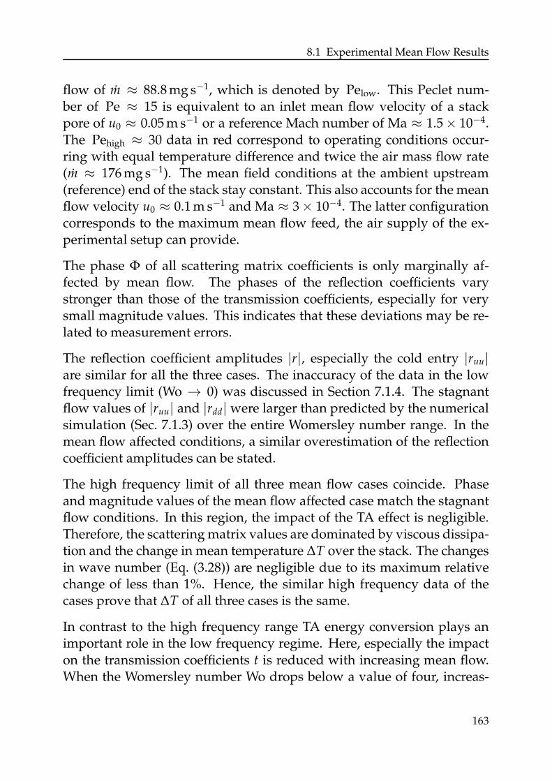
8.1 Experimental Mean Flow Results
flow of m ≈ 88.8 mg s−1, which is denoted by Pelow. This Peclet num-ber of Pe ≈ 15 is equivalent to an inlet mean flow velocity of a stackpore of u0 ≈ 0.05 m s−1 or a reference Mach number of Ma ≈ 1.5 × 10⁻⁴.The Pehigh ≈ 30 data in red correspond to operating conditions occur-ring with equal temperature difference and twice the air mass flow rate(m ≈ 176 mg s−1). The mean field conditions at the ambient upstream(reference) end of the stack stay constant. This also accounts for the meanflow velocity u0 ≈ 0.1 m s−1 and Ma ≈ 3 × 10⁻⁴. The latter configurationcorresponds to the maximum mean flow feed, the air supply of the ex-perimental setup can provide.
The phase Φ of all scattering matrix coefficients is only marginally af-fected by mean flow. The phases of the reflection coefficients varystronger than those of the transmission coefficients, especially for verysmall magnitude values. This indicates that these deviations may be re-lated to measurement errors.
The reflection coefficient amplitudes |r|, especially the cold entry |ruu|are similar for all the three cases. The inaccuracy of the data in the lowfrequency limit (Wo → 0) was discussed in Section 7.1.4. The stagnantflow values of |ruu| and |rdd| were larger than predicted by the numericalsimulation (Sec. 7.1.3) over the entire Womersley number range. In themean flow affected conditions, a similar overestimation of the reflectioncoefficient amplitudes can be stated.
The high frequency limit of all three mean flow cases coincide. Phaseand magnitude values of the mean flow affected case match the stagnantflow conditions. In this region, the impact of the TA effect is negligible.Therefore, the scattering matrix values are dominated by viscous dissipa-tion and the change in mean temperature ∆T over the stack. The changesin wave number (Eq. (3.28)) are negligible due to its maximum relativechange of less than 1%. Hence, the similar high frequency data of thecases prove that ∆T of all three cases is the same.
In contrast to the high frequency range TA energy conversion plays animportant role in the low frequency regime. Here, especially the impacton the transmission coefficients t is reduced with increasing mean flow.When the Womersley number Wo drops below a value of four, increas-
163
8 Impact of Mean Flow on the Scattering Behavior of TA Stacks
ing mass flow rates cause a stronger trend towards unity for both |tud|and |tdu|. This trend supports empirical observations [158, 159, 187] thatthe performance of a TA device drops with increasing mean flow andstops working before the temperature profile is “blown off”. The ob-served deviations in gain of more than 10% justify invoking direct meanflow interaction in one-dimensional prediction tools, although closure as-sumptions have to be drawn and the numerical effort increases.
8.2 CFD/SI Mean Flow Results
The CFD results of stagnant mean flow (black) and the Pehigh case aredisplayed in Figure 8.2. The intermediate case Pelow is skipped here.Instead, a second cases with the same upstream u0 conditions as Pehigh
is displayed. They only differ in their mean temperature profile. Pelin
000
000
1
1
22
22
44
44
66
66
88
88
1010
1010
0.1
0.1
0.2
0.2
0.3
0.3
0.4
0.4
0.6
0.7
0.8
0.9
1.1
1.2
1.3
1.4
Wo [−]Wo [−]
Wo [−]Wo [−]
|t ud|[−]
Φ(t
ud)[r
ad]
|t du|[−]
Φ(t
du)[r
ad]
|r dd|[−]
Φ(r
dd)[r
ad]
|r uu|[−]
Φ(r
uu)[r
ad]
ππ
ππ
π2
π2
π2
π2
00
00
-π2-π
2
-π2-π
2
-π-π
-π-π
|Pe0|
Φ( Pe0)
|Pelin |
Φ( Pelin)
|Peexp|
Φ(Peexp)
Figure 8.2: Scattering matrices obtained using the CFD/SI method for zero meanflow (black) and mean flow velocity of u0 = 0.1 m s−1 (red and blue). The latter twocases differ in their mean temperature profile, a conduction dominated case Pelin
(red) and a convection/diffusion case Peexp depicted in blue.
164
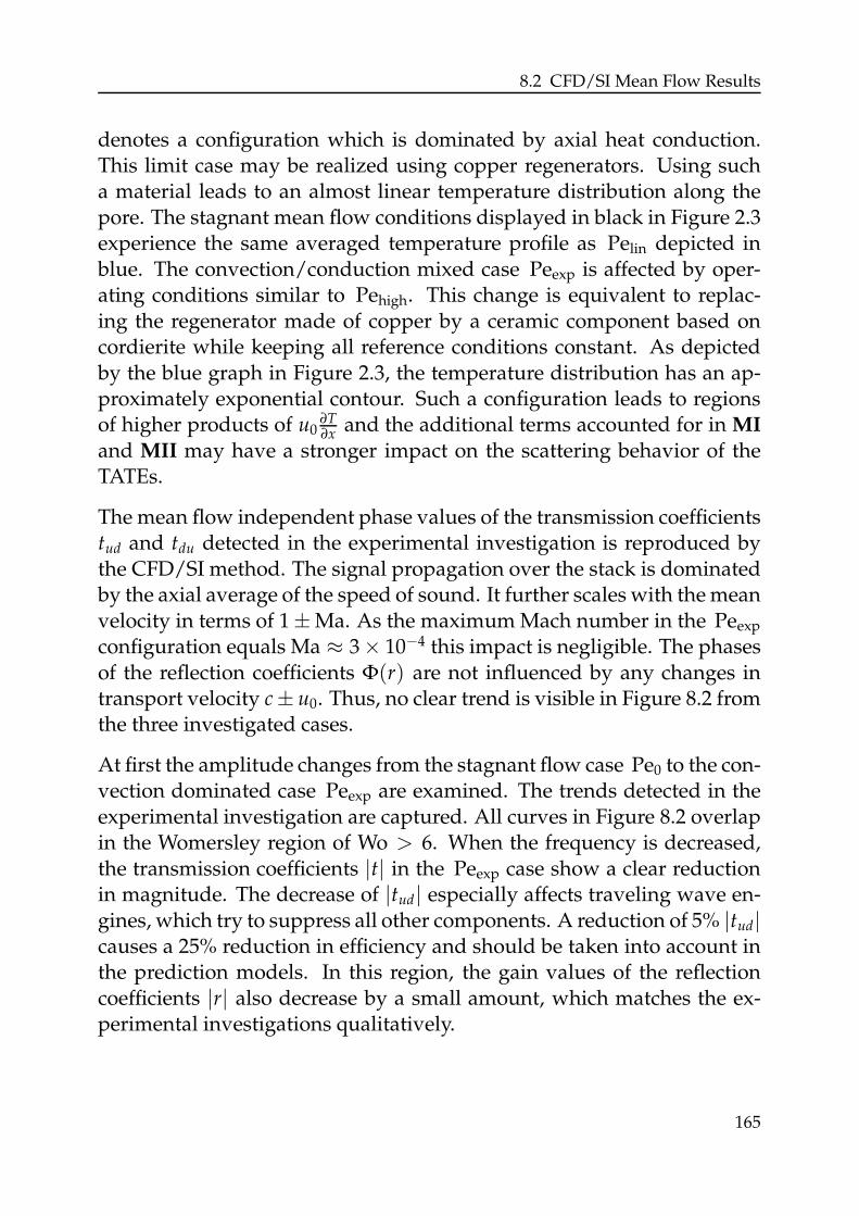
8.2 CFD/SI Mean Flow Results
denotes a configuration which is dominated by axial heat conduction.This limit case may be realized using copper regenerators. Using sucha material leads to an almost linear temperature distribution along thepore. The stagnant mean flow conditions displayed in black in Figure 2.3experience the same averaged temperature profile as Pelin depicted inblue. The convection/conduction mixed case Peexp is affected by oper-ating conditions similar to Pehigh. This change is equivalent to replac-ing the regenerator made of copper by a ceramic component based oncordierite while keeping all reference conditions constant. As depictedby the blue graph in Figure 2.3, the temperature distribution has an ap-proximately exponential contour. Such a configuration leads to regionsof higher products of u0
∂T∂x
and the additional terms accounted for in MI
and MII may have a stronger impact on the scattering behavior of theTATEs.
The mean flow independent phase values of the transmission coefficientstud and tdu detected in the experimental investigation is reproduced bythe CFD/SI method. The signal propagation over the stack is dominatedby the axial average of the speed of sound. It further scales with the meanvelocity in terms of 1 ± Ma. As the maximum Mach number in the Peexp
configuration equals Ma ≈ 3 × 10⁻⁴ this impact is negligible. The phasesof the reflection coefficients Φ(r) are not influenced by any changes intransport velocity c ± u0. Thus, no clear trend is visible in Figure 8.2 fromthe three investigated cases.
At first the amplitude changes from the stagnant flow case Pe0 to the con-vection dominated case Peexp are examined. The trends detected in theexperimental investigation are captured. All curves in Figure 8.2 overlapin the Womersley region of Wo > 6. When the frequency is decreased,the transmission coefficients |t| in the Peexp case show a clear reductionin magnitude. The decrease of |tud| especially affects traveling wave en-gines, which try to suppress all other components. A reduction of 5% |tud|causes a 25% reduction in efficiency and should be taken into account inthe prediction models. In this region, the gain values of the reflectioncoefficients |r| also decrease by a small amount, which matches the ex-perimental investigations qualitatively.
165
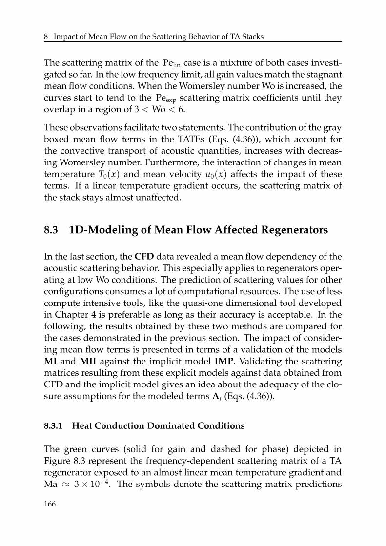
8 Impact of Mean Flow on the Scattering Behavior of TA Stacks
The scattering matrix of the Pelin case is a mixture of both cases investi-gated so far. In the low frequency limit, all gain values match the stagnantmean flow conditions. When the Womersley number Wo is increased, thecurves start to tend to the Peexp scattering matrix coefficients until theyoverlap in a region of 3 < Wo < 6.
These observations facilitate two statements. The contribution of the grayboxed mean flow terms in the TATEs (Eqs. (4.36)), which account forthe convective transport of acoustic quantities, increases with decreas-ing Womersley number. Furthermore, the interaction of changes in meantemperature T0(x) and mean velocity u0(x) affects the impact of theseterms. If a linear temperature gradient occurs, the scattering matrix ofthe stack stays almost unaffected.
8.3 1D-Modeling of Mean Flow Affected Regenerators
In the last section, the CFD data revealed a mean flow dependency of theacoustic scattering behavior. This especially applies to regenerators oper-ating at low Wo conditions. The prediction of scattering values for otherconfigurations consumes a lot of computational resources. The use of lesscompute intensive tools, like the quasi-one dimensional tool developedin Chapter 4 is preferable as long as their accuracy is acceptable. In thefollowing, the results obtained by these two methods are compared forthe cases demonstrated in the previous section. The impact of consider-ing mean flow terms is presented in terms of a validation of the modelsMI and MII against the implicit model IMP. Validating the scatteringmatrices resulting from these explicit models against data obtained fromCFD and the implicit model gives an idea about the adequacy of the clo-sure assumptions for the modeled terms Λi (Eqs. (4.36)).
8.3.1 Heat Conduction Dominated Conditions
The green curves (solid for gain and dashed for phase) depicted inFigure 8.3 represent the frequency-dependent scattering matrix of a TAregenerator exposed to an almost linear mean temperature gradient andMa ≈ 3 × 10⁻⁴. The symbols denote the scattering matrix predictions
166
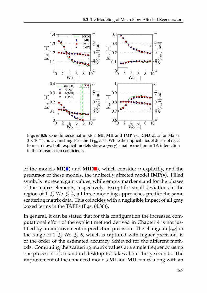
8.3 1D-Modeling of Mean Flow Affected Regenerators
000
000
1
1
22
22
44
44
66
66
88
88
1010
1010
0.1
0.1
0.2
0.2
0.3
0.3
0.4
0.4
0.6
0.7
0.8
0.9
1.1
1.2
1.3
1.4
Wo [−]Wo [−]
Wo [−]Wo [−]
|t ud|[−]
Φ(t
ud)[r
ad]
|t du|[−]
Φ(t
du)[r
ad]
|r dd|[−]
Φ(r
dd)[r
ad]
|r uu|[−]
Φ(r
uu)[r
ad]
ππ
ππ
π2
π2
π2
π2
00
00
-π2-π
2
-π2-π
2
-π-π
-π-π
|CFD|
Φ(CFD)
|MI|
Φ(MI)
|MII|
Φ(MII)
|IMP|
Φ(IMP)
Figure 8.3: One-dimensional models MI, MII and IMP vs. CFD data for Ma ≈3 × 10⁻⁴ and a vanishing Pe – the Pelin case. While the implicit model does not reactto mean flow, both explicit models show a (very) small reduction in TA interactionin the transmission coefficients.
of the models MI() and MII(), which consider u explicitly, and theprecursor of these models, the indirectly affected model IMP(•). Filledsymbols represent gain values, while empty marker stand for the phasesof the matrix elements, respectively. Except for small deviations in theregion of 1 . Wo . 4, all three modeling approaches predict the samescattering matrix data. This coincides with a negligible impact of all grayboxed terms in the TAPEs (Eqs. (4.36)).
In general, it can be stated that for this configuration the increased com-putational effort of the explicit method derived in Chapter 4 is not jus-tified by an improvement in prediction precision. The change in |tud| inthe range of 1 . Wo . 6, which is captured with higher precision, isof the order of the estimated accuracy achieved for the different meth-ods. Computing the scattering matrix values at a single frequency usingone processor of a standard desktop PC takes about thirty seconds. Theimprovement of the enhanced models MI and MII comes along with an
167
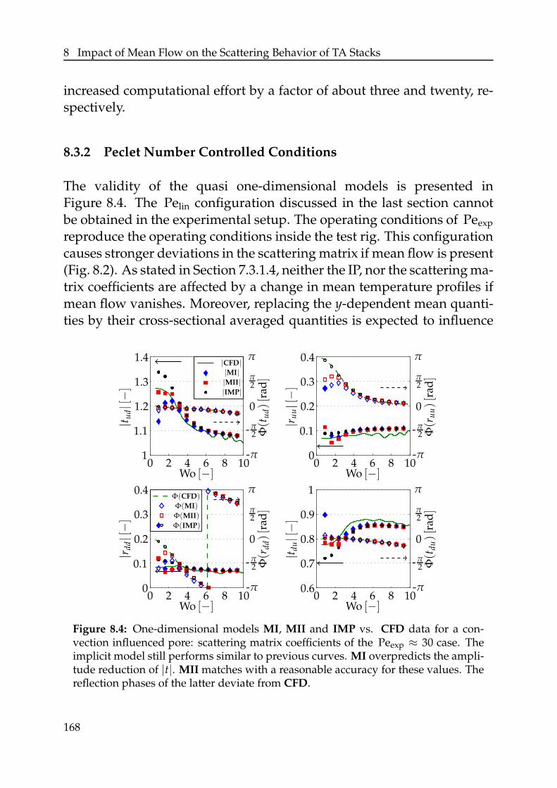
8 Impact of Mean Flow on the Scattering Behavior of TA Stacks
increased computational effort by a factor of about three and twenty, re-spectively.
8.3.2 Peclet Number Controlled Conditions
The validity of the quasi one-dimensional models is presented inFigure 8.4. The Pelin configuration discussed in the last section cannotbe obtained in the experimental setup. The operating conditions of Peexp
reproduce the operating conditions inside the test rig. This configurationcauses stronger deviations in the scattering matrix if mean flow is present(Fig. 8.2). As stated in Section 7.3.1.4, neither the IP, nor the scattering ma-trix coefficients are affected by a change in mean temperature profiles ifmean flow vanishes. Moreover, replacing the y-dependent mean quanti-ties by their cross-sectional averaged quantities is expected to influence
000
000
1
1
22
22
44
44
66
66
88
88
1010
1010
0.1
0.1
0.2
0.2
0.3
0.3
0.4
0.4
0.6
0.7
0.8
0.9
1.1
1.2
1.3
1.4
Wo [−]Wo [−]
Wo [−]Wo [−]
|t ud|[−]
Φ(t
ud)[r
ad]
|t du|[−]
Φ(t
du)[r
ad]
|r dd|[−]
Φ(r
dd)[r
ad]
|r uu|[−]
Φ(r
uu)[r
ad]
ππ
ππ
π2
π2
π2
π2
00
00
-π2-π
2
-π2-π
2
-π-π
-π-π
|CFD|
Φ(CFD)
|MI|
Φ(MI)
|MII|
Φ(MII)
|IMP|
Φ(IMP)
Figure 8.4: One-dimensional models MI, MII and IMP vs. CFD data for a con-vection influenced pore: scattering matrix coefficients of the Peexp ≈ 30 case. Theimplicit model still performs similar to previous curves. MI overpredicts the ampli-tude reduction of |t|. MII matches with a reasonable accuracy for these values. Thereflection phases of the latter deviate from CFD.
168
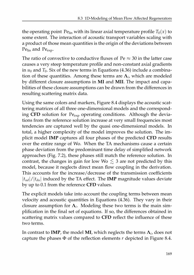
8.3 1D-Modeling of Mean Flow Affected Regenerators
the operating point Pelin with its linear axial temperature profile T0(x) tosome extent. The interaction of acoustic transport variables scaling witha product of those mean quantities is the origin of the deviations betweenPelin and Peexp.
The ratio of convective to conductive fluxes of Pe ≈ 30 in the latter casecauses a very steep temperature profile and non-constant axial gradientsin u0 and T0. Six of the new terms in Equations (4.36) include a combina-tion of these quantities. Among these terms are Λi, which are modeledby different closure assumptions in MI and MII. The impact and capa-bilities of these closure assumptions can be drawn from the differences inresulting scattering matrix data.
Using the same colors and markers, Figure 8.4 displays the acoustic scat-tering matrices of all three one-dimensional models and the correspond-ing CFD solution for Peexp operating conditions. Although the devia-tions from the reference solution increase at very small frequencies mosttendencies are captured well by the quasi one-dimensional models. Intotal, a higher complexity of the model improves the solution. The im-plicit model IMP captures all four phases of the predicted CFD resultsover the entire range of Wo. When the TA mechanisms cause a certainphase deviation from the predominant time delay of simplified networkapproaches (Fig. 7.2), these phases still match the reference solution. Incontrast, the changes in gain for low Wo . 3 are not predicted by thismodel, because it neglects direct mean flow coupling in the derivation.This accounts for the increase/decrease of the transmission coefficients|tud|/|tdu| induced by the TA effect. The IMP magnitude values deviateby up to 0.1 from the reference CFD values.
The explicit models take into account the coupling terms between meanvelocity and acoustic quantities in Equations (4.36). They vary in theirclosure assumption for Λi. Modeling these two terms is the main sim-plification in the final set of equations. If so, the differences obtained inscattering matrix values compared to CFD reflect the influence of thesetwo terms.
In contrast to IMP, the model MI, which neglects the terms Λi, does notcapture the phases Φ of the reflection elements r depicted in Figure 8.4.
169
8 Impact of Mean Flow on the Scattering Behavior of TA Stacks
Especially the low frequency region, i.e. Wo < 3, is not captured at all be-cause deviations in Φ of up to −π occur in this region. The crucial trans-mission coefficients |t| match for a wider region than for the IMP model.Contrary to all other results obtained, the model tends to the lower limitvalues of the temperature change (Eq. (7.2)) presented in Figure 7.2. Thismeans that the TA effect is predicted to totally break down for low fre-quencies using this closure assumption. The reference simulation doesnot share this trend. Thus, the closure terms Λi need to be considered.
Only MII takes these terms into account. Although the closure assump-tion is simplified severely, the transmission gain values match very wellin the critical region of Wo < 3. The absolute deviation in |tud| and |tdu|between the quasi one-dimensional model and the CFD data is reducedby one order of magnitude, while the phase of these components stayscomparable to CFD. The phase and gain error of the reflection coeffi-cients is also reduced by a factor of approximately two. The errors stillincrease with decaying Womersley numbers Wo.
Summarizing the validation of the one-dimensional models, a stepwiseimprovement in prediction accuracy is visible for the enhanced modelingof MI and MII. Taking into account mean flow in the TAPEs (Eqs. (4.36))is crucial for a better prediction. Especially a valid closure assumptionfor the terms Λi is necessary for a good description of the low Womersleyregion of cases with high Peclet numbers. Modeling these terms by across-sectional average of the IMP solution, i.e. MII, causes a reductionof 50% in magnitude error relative to MI. Except for the low frequencylimit, MII performs very accurate. In this region, the more sophisticatedapproaches discussed in Section 4.5.4 have to be used for achieving highaccuracy.
170
9 Conclusions and Outlook
The impact of laminar mean flow on acoustic scattering in TA regen-erators has been investigated. A quasi one-dimensional approach waspresented. Two closure assumptions were derived for an analytical ap-proach. The accuracy of the modeling approaches has been validatedagainst CFD data and results obtained experimentally for one test con-figuration.
The validation succeeded for stagnant mean flow conditions with onlylittle deviation for scattering matrix measurements as well as reconstruc-tion of the operating conditions of the experimental test rig in engineoperation mode. Due to the lack of reliability of the multi microphonemeasurements, the CFD solution was chosen as reference solution for avalidation of the quasi one-dimensional approach.
The second part of the validation was then carried out for mean flowaffected pores. The experimental data, CFD results and the analyticalmodeling revealed two key findings:
1. The TA effect occurring in regenerators is affected by mean flow ve-locity u0. For the settings considered, the transmission coefficientsof the scattering matrices showed an increasing sensitivity to meanflow for Mach numbers of Ma > 1.5 × 10⁻⁴. The change of TAinteraction is stronger if combinations of steep axial gradients inmean flow velocity u0(x) and mean temperature T0(x) occur insidethe pore. Thus, linear temperature profiles produce more acousticpower than convection-affected distributions T0(x), which, for ex-ample, occur in fluid/solid material combinations of air inside a ce-ramic regenerator. Linear temperature profiles are maintained bystack materials providing high conductivity. Such configurationsshow a TA scattering behavior similar to stagnant mean flow con-ditions. This is not valid for convection dominated cases. The inves-tigated combinations of mean flow and mean temperature distribu-
171
9 Conclusions and Outlook
tion cause a certain decay in the TA interaction. This corroboratesthe observations of other publications [158, 159].
2. The experimental results and multi-dimensional CFD simulationsshow a good agreement in the trends observed. These trends inthe CFD solution data can also be predicted by the quasi one-dimensional model. To find a good agreement, mean flow contri-bution has to be taken into account in the linearization process. Fur-ther, adequate closure assumptions have to be chosen. Here, espe-cially in the low Wo region, the advanced MII model showed betteragreement than IMP and MI. Only for very low Womersley numbersWo all tested closure assumptions fail. For the best model, MII thisfailure is restricted the phase of the reflection coefficients. Highercomplexity leads to higher accuracy, but is also accompanied by anincrease in computational effort. The same challenges arise with amore detailed description of the mean flow field.
The quasi one-dimensional model can be applied in numerical predictiontools in the early stage of the development of new technical setups. TheTA transport ODEs predict the spatial distribution of cross-sectionallyaveraged acoustic pressure and velocity distributions. Their validity isindependent of nonlinear effects as long as they only affect mean quan-tities. Thus the quasi one-dimensional models yield accurate predictionsof the acoustic performance of any TA device that is affected by meanflow.
The low-order model improves the prediction of acoustic transfer of alldevices marked by green dots in Figure 1.2 depicting the TA iceberg anal-ogy. It enables a more accurate prediction of the performance of devicesaffected by unwanted or deliberate mean flow. Streaming effects insideTA traveling wave applications can cause mean flow velocities compara-ble to the cases investigated in Chapter 8. These effects per se lead to areduction in conversion efficiency by causing losses and storing energyin second-order terms. The investigated examples show that these reduc-tions are even increased by the direct impact of mean flow on the acoustictransport equations. This shows the necessity of suppressing mean flowin such devices. The suppressing characteristic of mean flow velocitymay also be used to stabilize systems. For example, a small amount of
172
mean flow circulating in pipes entering and leaving the hydrogen stor-age of a fuel cell car can prevent the system from going unstable. Sucha measure improves the security of the energy supply in mobile appli-cations. Modeling the losses inside the supply system carefully facili-tates the application of the one-dimensional model derived to determinethe necessary amount of mean flow to stabilize the system. Finally, thedirect application of mean flow inside thermoacoustic devices may stillbe advantageous to traditional methods. Especially in waste heat con-version, where the heat is fed to the device by enthalpy flow, the directconversion of heat into acoustic power is attractive for potential appli-cation. The omission of one heat exchanger reduces the costs of the de-vice. These have to be balanced by the decrease in energy conversionefficiency, which is implied by the occurrence of mean flow inside theregenerator. Additionally, reducing the losses inside the system by omit-ting the heat exchanger may even lead to an improved performance ofthe overall setup. Computing this situation with the one-dimensionaltool leads to an accurate prediction of the expected efficiency of the sys-tem.
The low computational costs allow for a fast determination of the acoustictransfer for various configurations. Furthermore, applying it in combina-tion with the instability potentiality as optimization tool facilitates draw-ing a map that indicates the positive or negative impact of mean flow.The influence of several mean parameters shown in Section 7.3 demon-strates the multi-dimensionality of such a map. Tabulation methods andoptimization algorithms should be applied to ensure a fast determinationof promising operating conditions. Nevertheless, a technical device oper-ating with deliberate mean flow that improves the TA power conversionperformance remains unknown. The investigation of possible fields ofapplication is left to future research activity.
Finally, this thesis provides contributions that facilitate the understand-ing of the impact of mean flow on the TA effect. So far, Sondhauss andRijke type applications were clearly separated. Extending the use of theformer to the convective mean flow regime merges their applicability.This thesis does not show the differences and similarities of these energyconversion mechanisms. A close investigation may yield a combined ap-plication or demonstrate a familiarity of both effects that is not known
173

9 Conclusions and Outlook
today. It may lead to a new nomenclature distinguishing between con-duction and convection dominated acoustic power conversion.
174
Supervised Theses
Im Rahmen dieser Dissertation entstanden am Lehrstuhl fur Thermo-dynamik der TU Munchen in den Jahren 2007 bis 2012 unter wis-senschaftlicher, fachlicher und inhaltlicher Anleitung des Autors die imFolgenden aufgefuhrten studentischen Arbeiten. In ihnen wurden ver-schiedene Fragestellungen zur Warmeubergangsbestimmung und Ther-moakustik untersucht. Ergebnisse aus diesen Arbeiten konnen in Teilenin das vorliegende Dokument eingeflossen sein. Der Autor dankt hiermitnochmals explizit allen ehemals betreuten Studenten fur ihr Engagementbei der Unterstutzung dieser wissenschaftlichen Arbeit.
Associated with this Ph. D. thesis are a number of “student theses”(Semesterarbeiten, Diplomarbeiten, Bachelor theses or Master theses)that were supervised by the author of the present work. These theseswere prepared at the Lehrstuhl fur Thermodynamik at TU Munchen inthe years 2007 through 2012 under the close supervision of the presentauthor. Various issues were investigated concerning heat transfer prob-lems as well as thermoacoustic questions. Some parts of these supervisedtheses may have been incorporated into the present thesis. The authorwould like to express his sincere gratitude to all formerly supervised stu-dents for their commitment supporting this research project.
Student Thesis
AlexanderAvdonin
Determination of the Acoustic Power Generation Potential-ity of One-Dimensional Acoustic Elements, Semesterar-beit, filed in July 4th, 2011.
ArminBaumgartner
One-Dimensional Modeling of the Thermoacoustic Ef-fect Considering Mean Flow, Diplomarbeit, filed inNovember 15th, 2011.
175
9 Conclusions and Outlook
Stefan Erschen Konstruktion einer Thermoakustischen Maschine zur Un-tersuchung des Warmeubergangs in einer pulsieren-den Stromung (in German), Semesterarbeit, filed inAugust 24th 2009.
ViktorFleischer
Simulation und Systemidentifikation des thermoakustis-chen Effekts (in German), Semesterarbeit, filed inApril 26th, 2010.
RichardGurtner
Implementierung eines 1-D Modells zur Stabilitatsanalysethermoakustischer Stacks (in German), Semesterarbeit,filed in June, 8th 2010.
VeraHoferichter
Gittergenerierung und Optimierung zur Untersuchungthermoakustischer Grenzschichtphanomene (in German),Semesterarbeit, filed in August 31st, 2011.
ThomasKaiser
Numerical Simulation and System Identification of Ther-moacoustics, Semesterarbeit, filed in May 1st, 2011.
Claude Labonte& TobiasSachsenhauser
Numerische Parameterstudie des Warmeubergangs inpulsierenden Stromungen (in German), Semesterarbeit,filed in November 30st, 2007.
Jurgen Loth Thermische Identifikation und Optimierung eines Ther-moakustik Prufstandes (in German), Semesterarbeit,filed in June 15th, 2011.
ChristinaMauter
Aufbau und Inbetriebnahme eines Prufstandes zur Quan-tifizierung thermoakustischer Grenzschichteffekte (in Ger-man), Semesterarbeit, filed in Apritl 25th, 2011.
JohannesSchafer
Implementation of Non-Reflecting LODI Boundary Condi-tions with Plane Wave Masking in OpenFOAM , Semes-terarbeit, filed in April 15th, 2011.
Jurgen Stich Optimierung akustischer Simulationen fur Finite Volumenbasierte sequentielle Loser (in German), Semesterarbeit,filed in June 29, 2011.
176

MaximilianSperling
Numerical Computation of Acoustic Transfer in theLow Frequency Regime, Diplomarbeit, filed inNovember 15, 2012.
ConstanzeTemmler
Numerische Untersuchungen zum Einfluss derFestkorperwarmeleitung bei thermoakustischen Gren-zschichtphanomenen (in German), Bachelorthesis, filedin September 31st, 2011.
177

9 Conclusions and Outlook
178
References
[1] K. Abdoulla, Z. Yu, and A. J. Jaworski. Design of a Low-Cost Two-Stage Thermoacoustic Electricity Generator for Rural Communitiesin Developing Countries. In Proceedings of the 19th InternationalCongress on Sound and Vibration, Vilnius, Lithuania, July 2012.
[2] A. S. Abduljalil, Z. Yu, and A. J. Jaworski. Selection and Experi-mental Evaluation of Low-Cost Porous Materials for RegeneratorApplications in Thermoacoustic Engines. Materials & Design, 32(1):217–228, 2011.
[3] P. Aben, P. Bloemen, and J. Zeegers. 2-D PIV Measurements of Os-cillatory Flow Around Parallel Plates. Experiments in Fluids, 46:631–641, 2009.
[4] M. Abom and H. Boden. Error Analysis of Two–Microphone Mea-surements in Ducts with Flow. Journal of the Acoustical Society ofAmerica, 83(6):2429–2438, 1988.
[5] J. A. Adeff, T. J. Hofler, A. A. Atchley, and W. C. Moss. Measure-ments with Reticulated Vitreous Carbon Stacks in ThermoacousticPrime Movers and Refrigerators. Journal of the Acoustical Society ofAmerica, 104(1):32–38, 1998.
[6] Agilent Technologies, Inc. Agilent 34970A Users Guide, 2003.
[7] P. R. Alemela. Measurement and Scaling of Acoustic Transfer Matri-ces of Premixed Swirl Flames. Ph. D. thesis, Technische UniversitatMunchen, Munchen, Germany, 2009.
[8] M. Altenbokum. Das Phanomen Thermoakustik: Praktische An-wendungen. Kalte, Luft und Klimatechnik, 12:26–28, 2008.
[9] W. P. Arnott, H. E. Bass, and R. Raspet. General Formulation ofThermoacoustics for Stacks Having Arbitrarily Shaped Pore CrossSections. Journal of the Acoustical Society of America, 90:3228–3237,1991.
179
REFERENCES
[10] R. Aster, B. Borchers, and C. Thurber. Parameter Estimation and In-verse Problems. Academic Press, 2nd edition, 2012.
[11] A. A. Atchley, H. E. Bass, and T. J. Hofler. Development of Non-linear Waves in a Thermoacoustic Prime Mover. In M. F. Hamiltonand D. T. Blackstock, editors, Frontiers in Nonlinear Acoustics: Pro-ceedings of the 12th ISNA, pages 603—-608. Elsevier Science, Lon-don, 1990.
[12] A. A. Atchley. Analysis of the Initial Buildup of Oscillations in aThermoacoustic Prime Mover. Journal of the Acoustical Society ofAmerica, 95(3):1661–1664, 1994.
[13] Y. Auregan and R. Starobinski. Determination of Acoustical EnergyDissipation/Production Potentiality from the Acoustical TransferFunctions of a Multiport. Acta Acustica, 85(6):788–792, 1999.
[14] B. B. Efron and R. Tibshirani. An Introduction to the Bootstrap. Chap-man & Hall, 1993.
[15] S. Backhaus and G. W. Swift. A Thermoacoustic Stirling Heat En-gine. Nature, 399(6734):335–338, 1999.
[16] S. Backhaus and G. W. Swift. Fabrication and use of ParallelPlate Regenerators in Thermoacoustic Engines. In Proceedings of the36th Intersociety Energy Conversion Engineering Conference, Savannah,USA, pages 453–458, 2001.
[17] S. Backhaus and G. W. Swift. New Varieties of Thermoacoustic En-gines. In Proceedings of the 9th International Congress on Sound andVibration, Orlando, USA, pages 8–11, 2002.
[18] S. Backhaus and G. W. Swift. An Acoustic Streaming Instability inThermoacoustic Devices Utilizing Jet Pumps. Journal of the Acousti-cal Society of America, 113(3):1317–1324, 2003.
[19] S. Backhaus, G. W. Swift, and R. S. Reid. High-Temperature Self-Circulating Thermoacoustic Heat Exchanger. Applied Physics Let-ters, 87(1):14102–14102, 2005.
180
REFERENCES
[20] H. Bailliet, P. Lotton, M. Bruneau, V. Gusev, J. Valiere, and B. Gazen-gel. Acoustic Power Flow Measurement in a Thermoacoustic Res-onator by Means of Laser Doppler Anemometry (L.D.A.) and Mi-crophonic Measurement. Applied Acoustics, 60(1):1–11, 2000.
[21] H. Bailliet. Fascicule de Cours. In Ecole d’ete de thermoacoustique,Roscoff, France, pages 453–458, 2001.
[22] T. C. Bammann, C. Q. Howard, and B. Cazzolato. Review of Flow-Through Design in Thermoacoustic Refrigeration. In Proceedingsof the Australian Acoustical Society Conference, Busselton, Australia,pages 357–361, November 2005.
[23] A. Berson, M. Michard, and P. Blanc-Benon. Measurement ofAcoustic Velocity in the Stack of a Thermoacoustic Refrigerator Us-ing Particle Image Velocimetry. Heat and Mass Transfer, 44:1015–1023, 2008.
[24] R. B. Bird, W. E. Stewart, and E. N. Lightfoot. Transport Phenomena.Wiley, New York, 2nd edition, 2001.
[25] G. Bisio and G. Rubatto. Sondhauss and Rijke Oscil-lations—Thermodynamic Analysis, Possible Applications andAnalogies. Energy, 24(2):117–131, 1999.
[26] P. Blanc-Benon, E. Besnoin, and O. Knio. Experimental and Compu-tational Visualization of the Flow Field in a Thermoacoustic Stack.Comptes Rendus Mecanique, 331(1):17–24, 2003.
[27] H. Boden and M. A. bom. Influence of Errors on the Two-Microphone Method for Measuring Acoustic Properties in Ducts.Journal of the Acoustical Society of America, 79(2):541–549, 1986.
[28] D. Bohn and E. Deucker. An acoustical model to predict combus-tion driven oscillations. In 20th International Congress on CombustionEngines, 1993.
[29] E. Buckingham. On Physically Similar Systems: Illustrations of theUse of Dimensional Equations. Physical Review, 4(4):345–376, 1914.
[30] R. L. Carter and K. T. Feldman. An Acoustically Resonant StirlingEngine. pages 166–169, 1963.
181
REFERENCES
[31] P. H. Ceperley. A Pistonless Stirling Engine—The Traveling WaveHeat Engine. Journal of the Acoustical Society of America, 66(5):1508–1513, 1979.
[32] H. Chaitou, P. Nika, and G. Layes. A New Numerical OptimizationApproach For Standing-wave Thermoacoustic Engines. In Proceed-ings of the 19th International Congress on Sound and Vibration, Vilnius,Lithuania, July 2012.
[33] Chart BioMedical. QDrive-The Sound Choice. www.qdrive.com,2012.
[34] B. M. Chen, Y. A. Abakr, P. H. Riley, and D. B. Hann. Developmentof Thermoacoustic Engine Operating by Waste Heat from CookingStove. AIP Conference Proceedings, Sydney, Australia, 1440(1):532–540, 2012.
[35] G. B. Chen and T. Jin. Experimental Investigation on the Onset andDamping Behavior of the Oscillation in a Thermoacoustic PrimeMover. Cryogenics, 39(10):843–846, 1999.
[36] B.-T. Chu. On the Generation of Pressure Waves at a Plane FlameFront. International Symposium on Combustion, 4(1):603–612, 1953.
[37] J. R. Clement and J. Gaffney. Thermal Oscillations in low Tempera-ture Apparatus. Advances in Cryogenic Engineering, 1:302–306, 1953.
[38] K. D. Cole, J. V. Beck, A. Haji-Sheikh, and B. Litkouhi. Heat Condic-tion Using Green’s Functions. CRC Press, 2nd edition, 2011.
[39] T. Colonius and S. K. Lele. Computational Aeroacoustics: Progresson Nonlinear Problems of Sound Generation. Progress in AerospaceSciences, 40(6):345–416, 2004.
[40] COMSOL Multiphysics GmbH. COMSOL Multiphysics Users Guide,June 2012.
[41] C. Constanda. Solution Techniques for Elementary Partial DifferentialEquations. CRC Press, 2nd edition, 2010.
[42] Corning GmbH. Corning Thin-Wall Substrates, August 2012.
182
REFERENCES
[43] B. de Kees. Multi-Stage Travelling Wave Thermoacoustics in Prac-tice. In Proceedings of the 19th International Congress on Sound andVibration, Vilnius, Lithuania, July 2012.
[44] M. M. Denn. Process Fluid Mechanics. Prentice-Hall EnglewoodCliffs, NJ, 1980.
[45] A. P. Dowling. The Calculation of Thermoacoustic Oscillations.Journal of Sound and Vibration, 180(4):557–581, 1995.
[46] A. P. Dowling. Thermoacoustics and Instability. In Proceedings of the6th International Congress on Sound and Vibration, Copenhagen, Den-mark, 1999.
[47] A. P. Dowling and J. E. Ffowce-Williams. Sound and Sources of Sound.Ellis Horwoood, 1983.
[48] D. G. Duffy. Green’s Functions with Applications. Chapman &Hall/CRC, 2001.
[49] E. N. Economou and P. Fulde. Green’s Functions in Quantum Physics,volume 7. Springer-Verlag New York, 1979.
[50] S. Evesque and W. Polifke. Low-order acoustic modelling for annu-lar combustors: Validation and inclusion of modal coupling: Powerfor land, sea and air. In Proceedings of ASME Turbo Expo 2002 Powerfor Land, Sea and Air, July 2002.
[51] K. T. Feldman. A Study of Heat Generated Pressure Oscillations in aClosed end Pipe. Ph. D. thesis, University of New Mexico, College ofEngineering, Bureau of Engineering Research, 1965.
[52] K. T. Feldman. Review of the Literature on Sondhauss Thermoa-coustic Phenomena. Journal of Sound and Vibration, 7(1):71–82, 1968.
[53] K. Feldman Jr. Review of the Literature on Rijke ThermoacousticPhenomena. Journal of Sound and Vibration, 7(1):83–89, 1968.
[54] R. Feynman, R. Leighton, and M. Sands. The Feynman Lectures onPhysics, Vol. I: The New Millennium Edition: Mainly Mechanics, Radi-ation, and Heat. Basic Books, 2011.
183
REFERENCES
[55] A. Fischer. Hybride, thermoakustische Charakterisierung von Drallbren-nern. Ph. D. thesis, Technische Universitat Munchen, 2004.
[56] A. Fischer, C. Hirsch, and T. Sattelmayer. Comparison of multi-microphone transfer matrix measurements with acoustic networkmodels of swirl burners. Journal of Sound and Vibration, 298(73-83):73–83, 2006.
[57] S. Foller and W. Polifke. Advances in Identification Techniques forAero-Acoustic Scattering Coefficients from Large Eddy Simulation. In Proceedings of the 18th International Congress on Sound and Vibra-tion, Rio de Janeiro, Brasil, 2011.
[58] S. Foller and W. Polifke. Identification of Aero-Acoustic Scatter-ing Matrices from Large Eddy Simulation: Application to a Sud-den Area Expansion of a Duct. Journal of Sound Vibration, 331(13):3096–3113, 2012.
[59] A. M. Fusco, W. C. Ward, and G. W. Swift. Two-Sensor Power Mea-surements in Lossy Ducts. Journal of the Acoustical Society of America,91(4):2229–2235, 1992.
[60] S. Garrett. Thermoacoustic Engines and Refrigerators. AmericanJournal of Physics, 72:11–17, 2004.
[61] A. Gentemann and W. Polifke. Scattering and Generation of Acous-tic Energy by a Premix Swirl Burner. In Proceedings of the Interna-tional Gas Turbine and Aeroengine Congress & Exposition, Montreal,Quebec, Canada, 2007.
[62] A. M. G. Gentemann, A. Fischer, S. Evesque, and W. Polifke. Acous-tic Transfer Matrix Reconstruction and Analysis for Ducts withSudden Change of Area. In Proceedings of the 9th AIAA/CEAS Aeroa-coustics Conference and Exhibit, Hilton Head, USA, 2003.
[63] A. Gentemann. Identifikation von akustischen Transfermatrizen undFlammenfrequenzgangen mittels Stromungssimulation. Ph. D. thesis,Technische Universitat Munchen, 2006.
[64] O. S. Graham and A. P. Dowling. Low-Order Modelling of the Re-sponse of Ducted Flames in Annular Geometries. In Proceedings ofASME Turbo Expo 2012, No. GT2012-68698, Copenhagen, DK, 2012.
184
REFERENCES
[65] G.R.A.S. Sound & Vibration. 1/4-inch Pressure Microphone Type 40BP,2004.
[66] M. Guedra, G. Penelet, P. Lotton, and J. Dalmont. Theoretical Pre-diction of the Onset of Thermoacoustic Instability from the Exper-imental Transfer Matrix of a Thermoacoustic Core. Journal of theAcoustical Society of America, 130(1):145–152, 2011.
[67] D. Havelock, S. Kuwano, and M. Vorlander. Handbook of Signal Pro-cessing in Acoustics, volume 1. Springer Verlag, 2008.
[68] H. Helmholtz. On the Sensations of Tone. Dover Publications, 1954.
[69] B. Higgins. On the Sound Produced by a Current of Hydrogen GasPassing Through a Tube. Journal of Natural Philosophy and ChemicalArts, 1:129, 1802.
[70] O. Hireche, C. Weisman, D. Baltean-Carles, P. Le Quere, andL. Bauwens. Low Mach Number Analysis of Idealized Thermoa-coustic Engines with Numerical Solution. Journal of the AcousticalSociety of America, 128:3438, 2009.
[71] T. Hofler. Thermoacoustic Refrigerator Design and Performance. Ph. D.thesis, University of California, San Diego, 1986.
[72] T. Holzinger and W. Polifke. Optimization of ThermoacousticStacks for Maximum Generation of Acoustic Energy. In Proceed-ings of the 19th International Congress on Sound and Vibration, Vilnius,Lithuania, July 2012.
[73] T. Holzinger, T. Emmert, and W. Polifke. Optimization of Ther-moacoustic Regenerators for a Maximum Generation of AcousticEnergy. (sbmitted to) Journal of the Acoustical Society of America, 2013.
[74] Y. Huang, J. Benesty, and J. Chen. Acoustic MIMO Signal Processing,volume 1. Springer Berlin, Germany, 2006.
[75] A. Huber. Impact of Fuel Supply Impedance and Fuel Staging on GasTurbine Combustion Stability. Ph. D. thesis, Technische UniversitatMunchen, 2009.
185
REFERENCES
[76] G. Huelsz and F. Lopez-Alquicira. Hot-Wire Anemometry inAcoustic Waves. Experiments in Fluids, 30:283–285, 2001.
[77] G. Huelsz and E. Ramos. On the Phase Difference of the Tempera-ture and Pressure Waves in the Thermoacoustic Effect. InternationalCommunications in Heat and Mass Transfer, 22(1):71–80, 1995.
[78] F. Ihlenburg. Finite Element Analysis of Acoustic Scattering, volume132. Springer, 1998.
[79] D. P. Incropera, Frank P.and DeWitt. Fundamentals of Heat and MassTransfer. John Wiley & Sons, 2002.
[80] P. in’t panhuis, S. Rienstra, J. Molenaar, and J. Slot. Weakly Non-linear Thermoacoustics for Stacks with Slowly Varying Pore Cross-Sections. Journal of Fluid Mechanics, 618:41–70, 2009.
[81] P. H. M. W. in’t panhuis. Mathematical Aspects of Thermoacoustics.Ph. D. thesis, Technische Universiteit Eindhoven, 2009.
[82] P. H. M. W. in’t panhuis, S. W. Rienstra, and J. Molenaar. System-atic Derivation of the Weakly Non-Linear Theory of Thermoacous-tic Devices Version II. Technical report, Dep. of Mathematics andComputer Science Technische Universiteit Eindhoven, 2009.
[83] R. I. Issa. Solution of the Implicitly Discretised Fluid Flow Equa-tions by Operator-Splitting. Journal of Computational Physics, 62(1):40–65, 1985.
[84] H. Jasak. Error Analysis and Estimation for the Finite Volume Methodwith Applications to Fluid Flows. Ph. D. thesis, University of London,1996.
[85] C. Jorg. Estimation of Rehomogenization of Acoustic Fields inDucts. Private Communication, 2011.
[86] R. Kaess, A. Huber, and W. Polifke. A Time-Domain ImpedanceBoundary Condition for Compressible Turbulent Flow. In Pro-ceedings of the 14th AIAA/CEAS Aeroacoustics Conference (29th AIAAAeroacoustics Conference), May 2008, Vancouver, Canada, 2008.
186
REFERENCES
[87] R. Kaess, W. Polifke, T. Poinsot, N. Noiray, D. Durox, T. Schuller,and S. Candel. CFD-Based Mapping of the Thermo-Acoustic Sta-bility of a Laminar Premix Burner. In Proceedings of the SummerProgram, 2008.
[88] R. Kaess. Thermoacoustic Stability Analysis from Open Loop Trans-fer Functions based on LES. Ph. D. thesis, Technische UniversitatMunchen, 2010.
[89] M. Karlsson and M. Abom. Aeroacoustics of T-Junctions - An Ex-perimental Investigation. Journal of Sound and Vibration, 329(10):1793–1808, 2010.
[90] O. D. Kellogg. Foundations of Potential Theory, volume 31. DoverPublications, 2010.
[91] J. F. Kenney and E. S. Keeping. Mathematics of Statistics, volume 1.Van Nostrand, 1947.
[92] G. R. Kirchhoff. Uber den Einfluss der Warmeleitung in einem Gaseauf die Schallbewegung. Annalen der Physik, 134(6):177–193, 1868.
[93] C. T. Knipp. A Possible Standard of Sound. Physical Reviews, 12:491–492, 1918.
[94] J. Kopitz, E. Broker, and W. Polifke. Characteristics-Based Filter forIdentification of Acoustic Waves in Numerical Simulation of Tur-bulent Compressible Flow. In Proceeding of the 12th InternationalCongress on Sound and Vibration, Lisbon, Portugal, 2007.
[95] J. Kopitz. Kombinierte Anwendung von Stromungssimulation, Net-zwerkmodellierung und Regelungstechnik zur Vorhersage thermoakustis-cher Instabilitaten. Ph. D. thesis, Technische Universitat Munchen,2007.
[96] H. A. Kramers. Vibrations of a Gas Column. Physica, 15 (11–12):971–984, 1949.
[97] H.-O. Kreiss. Initial Boundary Value Problems for Hyperbolic Sys-tems. Communications on Pure and Applied Mathematics, 23(3):277–298, 1970.
187
REFERENCES
[98] R. A. Kruger, D. R. Reinecke, and G. A. Kruger. ThermoacousticComputed Tomography-Technical Considerations. Medical Physics,26(9):1832–1837, 1999.
[99] P. Kuchment and L. Kunyansky. Mathematics of ThermoacousticTomography. European Journal of Applied Mathematics, 19(02):191–224, 2008.
[100] P. K. Kundu and I. M. Cohen. Fluid Mechanics. Elsevier AcademicPress, 3rd edition, 2004.
[101] C. Kunzer. Untersuchung der numerischen Eigenschaften unter-schiedlicher Diskretisierungsschemata in OpenFOAM. Master’sthesis, Technische Universitat Munchen, 2011.
[102] R. Lacombe, P. Moussou, S. Foeller, G. Jasor, W. Polifke, andY. Auregan. Experimental and Numerical Investigations on theWhistling Ability of an Orifice in a Flow Duct. In Proceedings of 17thInternational Congress on Sound and Vibration, Cairo, Egypt, 2010.
[103] L. D. Landau and E. M. Lifshitz. Fluid Mechanics. Pergamon, 1959.
[104] H. Langhaar. Steady Flow in the Transition Length of a StraightTube. Journal of Applied Mechanics, 9(2):55–58, 1942.
[105] C. Lawn. A Linear 1D Model for the Thermoacoustic Effect inthe Presence of Mean Flow. In Proceedings of the 19th InternationalCongress on Sound and Vibration, Vilnius, Lithuania, July 2012.
[106] R. Leandro, A. Huber, and W. Polifke. taX Manual, 2012.
[107] L. Ljung. System Identification. Wiley Online Library, 1999.
[108] G. Lodato, P. Domingo, and L. Vervisch. Three-DimensionalBoundary Conditions for Direct and Large-Eddy Simulation ofCompressible Viscous Flows. Journal of Computational Physics, 227(10):5105–5143, 2008.
[109] T. Y. Lung and A. G. Doige. A Time-Averaging Transient TestingMethod for Acoustic Properties of Piping Systems and Mufflerswith Flow. Journal of the Acoustical Society of America, 73(3):867–876,1983.
188
REFERENCES
[110] R. Lyons. Understanding Digital Signal Processing. Prentice Hall PTR,2004.
[111] Lytron GmbH. Lytron, July 2012.
[112] C. Marx. Uber das Tonen erhitzter glaserner Rohren. Journal furPraktische Chemie, 22(1):129–135, 1841.
[113] D. Marx and P. Blanc-Benon. Numerical Simulation of Stack-HeatExchangers Coupling in a Thermoacoustic Refrigerator. AIAA Jour-nal, 42(7):1338–1347, 2004.
[114] G. F. McLaughlin and J. J. Keller. Thermoacoustic oscillations incombustion chambers of gas turbines. AIAA Journal, 12(33):2280–2287, 1995.
[115] P. Merkli and H. Thomann. Thermoacoustic Effects in a ResonanceTube. Journal of Applied Mechanics, 70:161–177, 1975.
[116] S. Mitra and Y. Kuo. Digital Signal Processing: a Computer-Based Ap-proach, volume 2. McGraw-Hill New York, 2006.
[117] M. Miyamoto, Y. Ito, K. Takahashi, T. Takami, T. Kobayashi,A. Nishida, and M. Aoyagi. Numerical Study on Sound Vibrationof an Air-Reed Instrument with Compressible LES. arXiv preprintarXiv:1005.3413, 2010.
[118] M. Miyamoto, Y. Ito, K. Takahashi, T. Takami, T. Kobayashi,A. Nishida, and M. Aoyagi. Applicability of Compressible LES toReproduction of Sound Vibration of an Air-Reed Instrument. InProceedings of 20th International Symposium on Music Acoustics, Syd-ney and Katoomba, Australia, 2010.
[119] P. J. J. Montgomery and S. L. Garrett. Low-Cost Thermoacoustic Co-Generator for Biomass-Burning Cook Stoves. Journal of the Acousti-cal Society of America, 128(4):2347–2347, 2010.
[120] M. J. Moran, H. N. Shapiro, D. D. Boettner, and M. Bailey. Funda-mentals of Engineering Thermodynamics. Wiley, 2010.
[121] I. Muller and W. Muller. Fundamentals of Thermodynamics and Appli-cations: with Historical Annotations and Many Citations From Avogadroto Zermelo. Springer, 2009.
189
REFERENCES
[122] M. L. Munjal. Acoustics of Ducts and Mufflers. John Wiley & Sons,1987.
[123] M. L. Munjal and A. G. Doige. Theory of a Two Source-LocationMethod for Direct Experimental Evaluation of the Four-Pole Pa-rameters of an Aeroacoustic Element. Journal of Sound and Vibration,141(2):323–333, 1990.
[124] National Institute of Standards and Technology (NIST). NISTChemistry WebBook, November 2008.
[125] K. A. Naugolnykh and L. A. Ostrovsky. Nonlinear Wave Processes inAcoustics. Cambridge Univ Pr, 1998.
[126] U. Neunert, C. Hirsch, and T. Sattelmayer. A Novel Approach toDetermine the Acoustic Transfer Matrices of Laminar Flat Flames.In Proceedings of the 4th European Combustion Meeting, Vienna, Aus-tria, April 2009.
[127] U. Neunert. Thermoakustische Stabilitat einer Reisemobilheizung. Ph.D. thesis, Technische Universitat Munchen, 2010.
[128] J. A. L. a. Nijeholt, M. E. H. Tijani, and S. Spoelstra. Simulationof a Traveling-Wave Thermoacoustic Engine Using ComputationalFluid Dynamics. Journal of the Acoustical Society of America, 118(4):2265–2270, 2005.
[129] D. Noda and Y. Ueda. Temperature Difference Required for the Op-eration of a Vaporized-Water Thermoacoustic Engine. In Proceed-ings of the 19th International Congress on Sound and Vibration, Vilnius,Lithuania, July 2012.
[130] J. R. Olson and G. W. Swift. Similitude in Thermoacoustics. Journalof the Acoustical Society of America, 95(3):1405–1412, 1994.
[131] J. R. Olson and G. W. Swift. Acoustic Streaming in Pulse Tube Re-frigerators: Tapered Pulse Tubes. Cryogenics, 37(12):769–776, 1997.
[132] A. V. Oppenheim, R. W. Schafer, J. R. Buck, et al. Discrete-Time SignalProcessing, volume 2. Prentice Hall Upper Saddle River, 1989.
190
REFERENCES
[133] C. C. Paige and M. A. Saunders. A Bidiagonalization Algorithmfor Sparse Linear Equations and Least-Squares Problems. Technicalreport, DTIC Document, 1978.
[134] C. O. Paschereit and W. Polifke. Investigation of the Thermo-Acoustic Characteristics of a Lean Premixed Gas Turbine Burner. InProceedings of the International Gas Turbine and Aeroengine Congress &Exposition, 1998.
[135] C. O. Paschereit, B. B. H. Schuermans, W. Polifke, and O. Mattson.Measurement of transfer matrices and source terms of premixedflames. J. Eng. Gas Turbines and Power, 124(2):239–247, April 2002.Originally published as ASME 99-GT-133.
[136] G. Penelet, V. Gusev, P. Lotton, and M. Bruneau. Experimen-tal and Theoretical Study of Processes Leading to Steady-StateSound in Annular Thermoacoustic Engines. Physical Review E, 72(1):016625/1–13, 2005.
[137] G. Penelet, S. Job, V. Gusev, P. Lotton, and M. Bruneau. Dependenceof Sound Amplification on Temperature Distribution in AnnularThermoacoustic Engines. Acta Acustica united with Acustica, 91(3):567–577, 2005.
[138] G. Petculescu and L. A. Wilen. Thermoacoustics in a Single Porewith an Applied Temperature Gradient. Journal of the AcousticalSociety of America, 106(2):688–694, 1999.
[139] A. Pinaud. Uber eine neue Art der Ton-Erzeugung. Annalen derPhysik, 118(13):610–618, 1837.
[140] G. Penelet. Introduction a la Thermoacoustique. In Ecole d’ete dethermoacoustique, Roscoff, France, pages 1–56, 2001.
[141] T. Poinsot and D. Veynante. Theoretical and Numerical Combustion.RT Edwards, Inc., 2005.
[142] T. Poinsot and S. K. Lele. Boundary Conditions for Direct Sim-ulations of Compressible Viscous Flows. Journal of ComputationalPhysics, 101(1):104–129, 1992.
191
REFERENCES
[143] W. Polifke. Combustion Instabilities. In Advances in Aero-Acousticsand Applications, Von Karman Institute for Fluid Dynamics, Brussels,Belgium, Von Karman Institute, 2004.
[144] W. Polifke. Low-Order Analysis Tools for Aero- and Thermo-Acoustic Instabilities. In Advances in Aero-Acoustics and Thermo-Acoustics, Von Karman Institute for Fluid Dynamics, Brussels, Belgium,2010.
[145] W. Polifke. Thermo-Acoustic Instability Potentiality of a PremixBurners. In European Combustion Meeting, ECM2011, Munich, Ger-many, 2011.
[146] W. Polifke and A. Gentemann. Order and Realizability of ImpulseResponse Filters for Accurate Identification of Acoustic Multi-Portsfrom Transient CFD. International Journal of Acoustics and Vibration,9(3):139–148, 2004.
[147] W. Polifke and C. O. Paschereit. Determination of Thermo-AcousticTransfer Matrices by Experiment and Computational Fluid Dynam-ics. ERCOFTAC Bulletin, 38, September 1998.
[148] W. Polifke and C. Wall. Non-Reflecting Boundary Conditions forAcoustic Transfer Matrix Estimation with LES. Combustion Turbur-bulence Research, Annual Research Briefs, pages 345–356, 2002.
[149] W. Polifke, C. O. Paschereit, and K. Dobbeling. Constructive anddestructive interference of acoustic and entropy waves in a pre-mixed combustor with a choked exit. Int. J. of Acoustics and Vibra-tion, 6(3):1–38, 2001.
[150] W. Polifke, A. Poncet, C. O. Paschereit, and K. Dobbeling. Recon-struction of Acoustic Transfer Matrices by Instationary Computa-tional Fluid Dynamics. Journal of Sound and Vibration, 245(3):483–510, 2001.
[151] W. Polifke, A. Fischer, and T. Sattelmayer. Instability of a PremixBurner with Nonmonotonic Pressure Drop Characteristic. Journalof Engineering for Gas Turbines and Power, 125:1–8, 2003.
192
REFERENCES
[152] W. Polifke, C. Wall, and P. Moin. Partially Reflecting and Non-Reflecting Boundary Conditions for Simulation of CompressibleViscous Flow. Journal of Computational Physics, 213:437–449, 2006.
[153] T. L. Polles, M.-X. Francois, P. Duthil, and J.-P. Thermeau. Le Froidvenu du Son. La Gazette du Vide, 18:14–16, 2010.
[154] W. H. Press, S. A. Teukolsky, W. T. Vetterling, and B. P. Flannery.Numerical Recipes: The Art of Scientific Computing. Cambridge Uni-versity Press, 3rd edition, 2007.
[155] J. G. Proakis and D. G. Manolakis. Digital Signal Processing, vol-ume 99. Macmillan Publishing Company, New York, 1996.
[156] Promat GmbH. Promaform, June 2012.
[157] L. Rayleigh. The Theory of Sound, volume I & II. Macmillan and Co.,1878.
[158] R. S. Reid. Open Cycle Thermoacoustics. Ph. D. thesis, Los AlamosNational Laboratory, 2000.
[159] R. S. Reid, W. C. Ward, and G. W. Swift. Cyclic Thermodynamicswith Open Flow. Physical Review Letters, 80:4617–4620, 1998.
[160] S. W. Rienstra and A. Hirschberg. An Introduction to Acoustics.Eindhoven University of Technology, 2001.
[161] P. L. Rijke. Notiz uber eine neue Art, die in einer an beiden En-den offenen Rohre enthaltene Luft in Schwingungen zu versetzen.Annalen der Physik, 183(6):339–343, 1859.
[162] P. Riley. Stove for Cooking, Refrigeration and Electricity.http://www.score.uk.com/, 2009.
[163] T. D. Rossing, editor. Springer Hand Books of Acoustics. SpringerScience+Business Media, LLC New York, 2007.
[164] N. Rott. Damped and Thermally Driven Acoustic Oscillations inWide and Narrow Tubes. Zeitschrift fur angewandte Mathematik undPhysik, 20:230–243, 1969.
193
REFERENCES
[165] N. Rott. Thermally Driven Acoustic Oscillations. Part II: StabilityLimit for Helium. Zeitschrift fur angewandte Mathematik und Physik,24:54–72, 1973.
[166] N. Rott. The Heating Effect Connected with Non-linear Oscilla-tions in a Resonance Tube. Zeitschrift fur angewandte Mathematikund Physik, 25:619–634, 1974.
[167] N. Rott. Thermally Driven Acoustic Oscillations, Part III: Second-Order Heat Flux. Zeitschrift fur angewandte Mathematik und Physik,26:43–49, 1975.
[168] N. Rott. The Description of Simple Waves by Particle Displacement.Zeitschrift fur angewandte Mathematik und Physik, 29:178–189, 1978.
[169] N. Rott. The Mutual Penetration of Simple Waves in Gases.Zeitschrift fur angewandte Mathematik und Physik, 29:462–472, 1978.
[170] N. Rott. Thermoacoustics. In Advances in Applied Mechanics, vol-ume 20, pages 135–175. Elsevier, 1980.
[171] N. Rott and G. Zouzoulas. Thermally Driven Acoustic Oscillations,Part IV: Tubes with Variable Cross-section. Zeitschrift fur angewandteMathematik und Physik, 27:197–224, 1976.
[172] D. H. Rudy and J. C. Strikwerda. A Nonreflecting Outflow Bound-ary Condition for Subsonic Navier-Stokes Calculations. Journal ofComputational Physics, 36(1):55–70, 1980.
[173] S. Sakamoto and Y. Watanabe. The Experimental Studies of Ther-moacoustic Cooler. Ultrasonics, 42(1–9):53–56, 2004.
[174] A. O. Santillan and R. R. Boullosa. Acoustic Power and Heat Fluxesin the Thermoacoustic Effect due to a Travelling Plane Wave. Inter-national Journal of Heat and Mass Transfer, 40(8):1835–1838, 1997.
[175] H. Schlichting, K. Gersten, E. Krause, H. Oertel, and K. Mayes.Boundary-Layer Theory. Springer Verlag, 8th edition, 2000.
[176] T. Schonfeld and T. Poinsot. Influence of Boundary Conditions inLES of Premixed Combustion Instabilities. Annual Research Briefs,pages 73–84, 1999.
194
REFERENCES
[177] B. Schuermans. Modelling and Control of Thermoacoustic Instabilities.Ph. D. thesis, Ecole Polytechnique Federale De Lausanne, 2003.
[178] B. Schuermans, F. Bellucci, V. Guethe, F. Meili, P. Flohr, and C. O.Paschereit. A detailed analysis of thermoacoustic interaction mech-anisms in a turbulent premixed flame. In Int’l Gas Turbine and Aero-engine Congress & Exposition, Atlanta, GA, U.S.A., June 14-17 2004.
[179] B. B. H. Schuermans, W. Polifke, and C. O. Paschereit. ModelingTransfer Matrices of Premixed Flames and Comparison with Ex-perimental Results. In Int’l Gas Turbine and Aeroengine Congress &Exposition, Indianapolis, Indiana, USA, 1999.
[180] B. B. H. Schuermans, W. Polifke, C. O. Paschereit, and J. H. van derLinden. Prediction of acoustic pressure spectra in combustion sys-tems using swirl stabilized gas turbine burners. In Proceedings of theIGTI, Munich, Germany, May 13-16 2000. ASME.
[181] L. Selle, F. Nicoud, and T. Poinsot. Actual Impedance of Nonreflect-ing Boundary Conditions: Implications for Computation of Res-onators. AIAA Journal, 42(5):958–964, 2004.
[182] C. Sondhauss. Uber die Schallschwingungen der Luft in erhitztenGlasrohren und in gedeckten Pfeifen von ungleicher Weite. Annalender Physik, 155(1):1–34, 1850.
[183] S. R. Stow and A. P. Dowling. Thermoacoustic oscillations in anannular combustor. In Proceedings of ASME Turbo Expo 2001 Powerfor Land, Sea and Air, New Orleans, Louisiana, June 4-7 2001. ASME.
[184] G. W. Swift. Analysis and Performance of a Large ThermoacousticEngine. Journal of the Acoustical Society of America, 92(3):1551–1563,1992.
[185] G. W. Swift. Thermoacoustic Engines and Refigerators. Encyclopediaof Applied Physics, Testing Equipment-Mechanical to Topological PhaseEffects, 21:22–28, 1995.
[186] G. W. Swift. Streaming in Thermoacoustic Engines and Refriger-ators. In AIP Conference Proceedings, Adelaide, Australia, December2000.
195
REFERENCES
[187] G. W. Swift. Thermoacoustics- A Unifying Perspective for Some Enginesand Refrigerators. Acoustical Society of America, 2002.
[188] G. W. Swift and S. Backhaus. A Resonant, Self-Pumped, CirculatingThermoacoustic Heat Exchanger. Journal of the Acoustic Society ofAmerica, 116 (5):2923–2938, 2004.
[189] G. W. Swift and W. C. Ward. Simple Harmonic Analysis of Regen-erators. Journal of Thermophysics and Heat Transfer, 10(4):652–662,1996.
[190] K. W. Taconis. Vapor-Liquid Equilibrium of Solutions of 3He in4He. Physica, 15:738, 1949.
[191] K. Takahashi, M. Miyamoto, Y. Ito, T. Takami, T. Kobayashi,A. Nishida, and M. Aoyagi. Numerical Analysis on 2D and 3DEdge Tones in Terms of Aerodynamic Sound Theory. In Proceedingsof 20th International Congress on Acoustics, Sydney, Australia, 2010.
[192] L. R. Tay-Wo-Chong Hilares. Numerical Simulation of the Dynamicsof Turbulent Swirling Flames. Ph. D. thesis, Technische UniversitatMunchen, 2012.
[193] J. R. Taylor. An Introduction to Error Analysis: the Study of Uncertain-ties in Physical Measurements. Universal Science Books, 1997.
[194] P. Testud, Y. Auregan, P. Moussou, and A. Hirschberg. TheWhistling Potentiality of an Orifice in a Confined Flow Using anEnergetic Criterion. Journal of Sound and Vibration, 325(4):769–780,2009.
[195] K. W. Thompson. Time Dependent Boundary Conditions for Hy-perbolic Systems. Journal of Computational Physics, 68(1):1–24, 1987.
[196] K. W. Thompson. Time Dependent Boundary Conditions for Hy-perbolic Systems, II. Journal of Computational Physics, 89(2):439–461,1990.
[197] H. Tijdeman. On the Propagation of Sound Waves in CylindricalTubes. Journal of Sound and Vibration, 39(1):1–33, 1975.
196
REFERENCES
[198] C. W. S. To and A. G. Doige. A Transient Testing Technique for theDetermination of Matrix Parameters of Acoustic Systems, I: Theoryand Principles. Journal of Sound and Vibration, 62(2):207–222, 1979.
[199] C. To and A. Doige. A Transient Testing Technique for the Determi-nation of Matrix Parameters of Acoustic Systems, II: ExperimentalProcedures and Results. Journal of Sound and Vibration, 62(2):223–233, 1979.
[200] A. Ulhaq, S. Hemchandra, L. Tay-Wo-Chong, and W. Polifke.Multiple-Input, Single-Output Approach for Identification of Lam-inar Premixed Flame Dynamics from Direct Numerical Simulation.In Proceedings of the 19th International Congress on Sound and Vibra-tion, Vilnius, Lithuania, July 2012.
[201] V.-G. V. und Chemieingenieurwesen (GVC), editor. VDI-Warmeat-las. VDI-Verlag, Dusseldorf, 8th edition, 2007.
[202] B. Ward, J. Clark, and G. W. Swift. DeltaEC Version 6.2 Users Guide.Technical report, Los Alamos National Laboratory, 2008.
[203] W. Ward and G. Swift. Design Environment for Low–AmplitudeThermoacoustic Engines. Journal of the Acoustical Society of America,95(6):3671–3674, 1994.
[204] M. Watanabe, A. Prosperetti, and H. Yuan. A Simplified Model forLinear and Nonlinear Processes in Thermoacoustic Prime Movers.Part I. Model and Linear Theory. Journal of the Acoustical Society ofAmerica, 102(6):3484–3496, 1997.
[205] N. T. Weiland. Feasibility Analysis of an Open Cycle ThermoacousticEngine with Internal Pulse Combustion. Ph. D. thesis, Georgia Insti-tute of Technology, 2004.
[206] J. Wheatley, T. Hofler, G. W. Swift, and A. Migliori. An IntrinsicallyIrreversible Thermoacoustic Heat Engine. Journal of the AcousticalSociety of America, 74(1):153–170, 1983.
[207] J. Wheatley, G. W. Swift, and A. Migliori. The Natural Heat Engine.Los Alamos Science, 14:2–47, 1986.
197
REFERENCES
[208] N. Wiener. Extrapolation, Interpolation, and Smoothing of Station-ary Time Series: with Engineering Applications. Journal of the Amer-ican Statistical Association, 47(258), 1949.
[209] Wolfram Research. Mathematica, June 2012.
[210] A. S. Worlikar and O. M. Knio. Numerical Simulation of a Ther-moacoustic Refrigerator. Journal of Computational Physics, 127(2):424–451, 1995.
[211] A. S. Worlikar, O. M. Knio, and R. Klein. Numerical Simulation of aThermoacoustic Refrigerator: II. Stratified Flow Around the Stack.Journal of Computational Physics, 144(2):299–324, 1998.
[212] T. Yazaki, A. Iwata, T. Maekawa, and A. Tominaga. Traveling WaveThermoacoustic Engine in a Looped Tube. Physical Review Letters,81:3128–3131, October 1998.
[213] C. S. Yoo and H. G. Im. Characteristic Boundary Conditionsfor Simulations of Compressible Reacting Flows with Multi-Dimensional, Viscous and Reaction Effects. Combustion Theory andModelling, 11(2):259–286, 2007.
[214] C. S. Yoo, Y. Wang, A. Trouve, and H. G. Im. Characteristic Bound-ary Conditions for Direct Simulations of Turbulent CounterflowFlames. Combustion Theory and Modelling, 9(4):617–646, 2005.
[215] G. Y. Yu, E. C. Luo, W. Dai, and J. Y. Hu. Study of Nonlinear Pro-cesses of a Large Experimental Thermoacoustic Stirling Heat En-gine by Using Computational Fluid Dynamics. Journal of AppliedPhysics, 102(7):074901, 2007.
[216] H. Yuan, S. Karpov, and A. Prosperetti. A Simplified Model forLinear and Nonlinear Processes in Thermoacoustic Prime Movers.Part II. Nonlinear Oscillations. Journal of the Acoustical Society ofAmerica, 102(6):3497–3506, 1997.
[217] S. Zhou and Y. Matsubara. Experimental Research of Thermoacous-tic Prime Mover. Cryogenics, 38(8):813–822, 1998.
[218] J. Zierep. Theoretical Gasdynamics. Springer-Verlag, 1978.
198
REFERENCES
[219] F. Zink, J. Vipperman, and L. Schaefer. CFD Simulation of a Ther-moacoustic Engine with Coiled Resonator. International Communi-cations in Heat and Mass Transfer, 37(3):226–229, 2010.
[220] F. Zink, J. Vipperman, and L. Schaefer. CFD Simulation of Ther-moacoustic Cooling. International Journal of Heat and Mass Transfer,53(19–20):3940–3946, 2010.
[221] D. Zwillinger. Handbook of Differential Equations. Academic Press,3rd edition, 1998.
199

REFERENCES
200
A Details of the Derivation of the Quasi 1D-Model
This chapter contains details of the derivation shown in Chapter 4. Thespecial non-dimenzionalization technique applied yields a dimensionlesssystem of equations in different orders of ε, i.e. the pore aspect ratio. Dueto this ratio such terms of higher order are later neglected and, for betterreadability, presented in the main text with abbreviations Ai
(O(ε2))
. Inthe following chapter, these terms are presented. The derivation of thequasi one-dimensional explicit TAPEs (Eqs. (4.63)) causes an increase innumber of terms of the implicit solution. For the purpose of giving anoverview of the derivation steps, these terms are accumulated to replace-ment parameters. In the second part of this chapter, these parameters aregiven in detail.
A.1 Higher Order Terms in the Dimensionless NSEs
The formulation of the LNSEs (Eqs. (4.9)) contain various termsAi
(O(ε2))
which are later neglected.
The second and higher order contribution in ε to the axial momentumEquation (4.9b) reads
A1
(O(ε2))
= ε2
[
κ
Wo2
(
2∂2u
∂x2+
∂2v
∂x∂y
)
+κ
Wo2ζ
(∂2u
∂x2+
∂2v
∂x∂y
)]
+ ε3 κ
Wo2
∂2v
∂x2. (A.1)
The spatial derivatives and the scaling with Wo indicate the origin of theterms. All terms in A1
(O(ε2))
result from viscous stress tensor τij.
201
A Details of the Derivation of the Quasi 1D-Model
The transversal momentum Equation (4.9c) is multiplied by ε to obtainzeroth order information. Thus,
A2
(O(ε2))
= ε2
[
Dv
Dt+
κ
Wo2
(
2∂2v
∂y2+
∂2u
∂x∂y
)
+κ
Wo2ζ
(∂2v
∂y2+
∂2u
∂x∂y
)]
+ ε3
[
3κ
Wo2
∂2v
∂x∂y+
κ
Wo2ζ
(∂2u
∂x2+
∂2v
∂x∂y
)]
(A.2)
additionally contains the substantial derivative of the transversal veloc-ity.
Both the fluid energy conservation (Eq. (4.9d)) and the solid energy con-servation (Eq. (4.9f)) further include the axial thermal conductivity termin
A3
(O(ε2))
= ε2
[
2κ
Wo2
([∂v
∂y+
∂u
∂x
]2
+∂u
∂y
∂v
∂x
)
+κ
Wo2ζ
(∂v
∂y+
∂u
∂x
)2
+κ
2La2
∂2T
∂x2
]
+ ε4 κ
Wo2
∂v
∂y
2
,
A4
(O(ε2))
= ε2 κ
2La2S
∂2T
∂x2, (A.3)
which is of higher order in ε. This is in accordance to the approach for thethermodynamic cycle stated in Section 1.2. It states that changes of thethermodynamic state in the vicinity of a thermo-viscous acoustic bound-ary layer are governed by transversal heat conduction, while the axialcontribution is negligible.
A.2 Abbreviations for the Analytical Approaches
The abbreviations introduced in Section 4.5.3 follow a nomenclaturebased on the original equation and contributing terms.
202
A.2 Abbreviations for the Analytical Approaches
A.2.1 Axial Momentum Equation
Comparing Equations (4.36c) and (4.39) under consideration ofEquation (4.37) directly leads to
Xp1=
(1 − γ) T
iκ − Ma∂T∂x
, (A.4)
XΛ1=
(1 − γ) TΛ1
iκ − Ma∂T∂x
. (A.5)
A.2.2 Energy Equation
Substituting the solution of Equation (4.39) into Equation (4.36e) leads tothe abbreviations
Ep1=
T((−1 + γ) κ − icpMaγ∂T
∂x
)
cp
(κ − iMa ∂T
∂x
) , (A.6)
Ep1,Fν = 0, (A.7)
Ep′1= −(Ma (−1 + γ) T2
cp
(iκ + Ma∂T
∂x
) , (A.8)
Ep′1,Fν= − Xp1
∂T∂x
iκ + Ma∂T∂x
, (A.9)
EΛ2=
i (−1 + γ) TΛ2
cp
(κ − iMa ∂T
∂x
) , (A.10)
EΛ1,Fν =−XΛ1
∂T∂x
iκ + Ma∂T∂x
. (A.11)
Here, the terms EΛ2and EΛ1,Fν vanish for MI. After combining the energy
Equations (4.36e) and (4.36f) the new variables occurring are
Tp1=
(
PrEp1+ Ep1,Fν
(
−1 +fK,ν
fK
))
EǫS, (A.12)
Tp′1=
(
PrEp′1+ Ep′1,Fν
(
−1 +fK,ν
fK
))
EǫS, (A.13)
TΛ1= − (EΛ1,FνEǫS
) +(PrEΛ2
fK + EΛ1,Fν fK,ν)EǫS
fK, (A.14)
203
A Details of the Derivation of the Quasi 1D-Model
Tp1,FK=
Ep1,Fν ( fK − fK,ν)EǫS+ Ep1
fK (1 −PrEǫS)
fK, (A.15)
Tp′1,FK=
Ep′1,Fν( fK − fK,ν)EǫS
+ Ep′1fK (1 −PrEǫS
)
fK, (A.16)
TΛ2FK=
EΛ1,Fν ( fK − fK,ν)EǫS
fK+ EΛ2 (1 −PrEǫS
) . (A.17)
It needs to be emphasized that all of these terms include contributionsof EǫS
indicating of the fluid-solid interaction. This index is discharged.Again, Equations (A.14) and (A.17) are zero for the less accurate modelMI.
A.2.3 Gas Law
The first substitution process of the resulting energy Equation (4.58) andmomentum Equation (4.39) into the ideal gas Equation (4.36a) yields twonew parameters
Gp1=
γ
(−1 + γ) T, (A.18)
GT1=
−1
(−1 + γ) T2, (A.19)
which are combined to
Gp1= Gp1
+(Ep1,Fν + Tp1
+ Tp1,FK− Tp1,FK
fK − Ep1,Fν fK,ν
)GT1
,
(A.20)
Gp′1=(
Ep′1,Fν+ Tp′1
+ Tp′1,FK− Tp′1,FK
fK − Ep′1,FνfK,ν
)
GT1, (A.21)
GΛ1,Λ2= (TΛ1
+ TΛ2FK+ EΛ1,Fν − TΛ2FK
fK − EΛ1,Fν fK,ν)GT1(A.22)
in the cross-sectional averaging process. Again the last term is zero forMI.
204
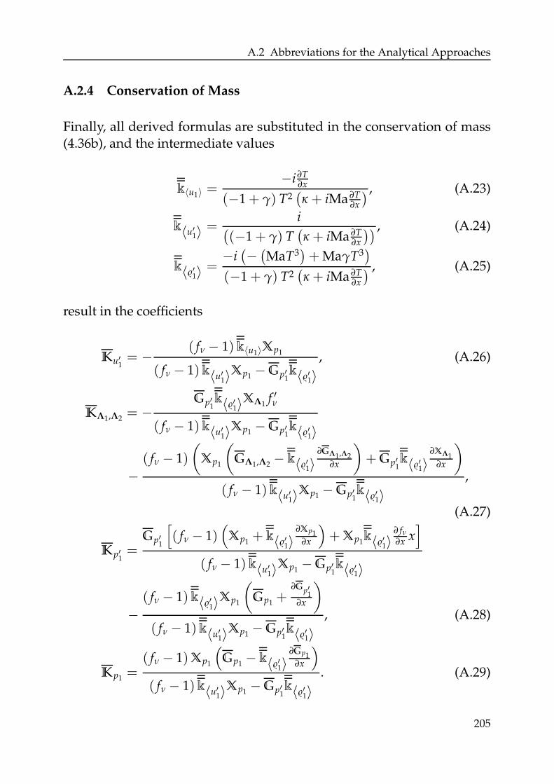
A.2 Abbreviations for the Analytical Approaches
A.2.4 Conservation of Mass
Finally, all derived formulas are substituted in the conservation of mass(4.36b), and the intermediate values
k〈u1〉 =−i ∂T
∂x
(−1 + γ) T2(κ + iMa ∂T
∂x
) , (A.23)
k〈u′1〉 =i
((−1 + γ) T
(κ + iMa ∂T
∂x
)) , (A.24)
k〈′1〉 =−i(−(MaT3
)+ MaγT3
)
(−1 + γ) T2(κ + iMa ∂T
∂x
) , (A.25)
result in the coefficients
Ku′1= − ( fν − 1) k〈u1〉Xp1
( fν − 1) k〈u′1〉Xp1− Gp′1
k〈′1〉, (A.26)
KΛ1,Λ2= −
Gp′1k〈′1〉XΛ1
f ′ν
( fν − 1) k〈u′1〉Xp1− Gp′1
k〈′1〉
−( fν − 1)
(
Xp1
(
GΛ1,Λ2− k〈′1〉
∂GΛ1,Λ2∂x
)
+ Gp′1k〈′1〉
∂XΛ1∂x
)
( fν − 1) k〈u′1〉Xp1− Gp′1
k〈′1〉,
(A.27)
Kp′1=
Gp′1
[
( fν − 1)(
Xp1+ k〈′1〉
∂Xp1∂x
)
+ Xp1k〈′1〉
∂ fν
∂x x]
( fν − 1) k〈u′1〉Xp1− Gp′1
k〈′1〉
−( fν − 1) k〈′1〉Xp1
(
Gp1+
∂Gp′1
∂x
)
( fν − 1) k〈u′1〉Xp1− Gp′1
k〈′1〉, (A.28)
Kp1=
( fν − 1)Xp1
(
Gp1− k〈′1〉
∂Gp1∂x
)
( fν − 1)k〈u′1〉Xp1− Gp′1
k〈′1〉. (A.29)
205

A Details of the Derivation of the Quasi 1D-Model
The second transport ODE of the acoustic variables (see Eqs. (4.63)) isdenoted in terms of these coefficients. The term KΛ1,Λ2
contains the termsdiffering in the different model derivations.
206
B Experimental Modeling Approaches
The experimental investigation of TA regenerators in Chapter 6 necessi-tates the introduction of two modeling approaches. The hot downstreamdata acquisition region is governed by non-negligible changes in meantemperature T. As the test rig only allows for local temperature prob-ing, the axial distribution is modeled. The scattering matrices obtainedinclude the acoustic transmission behavior of the adjacent heaters. Thistransmission behavior is reconstructed from separate measurements. Asthe final solution is — to some extent — sensitive to this data, the re-constructed scattering matrices are modeled analytically before they areapplied to obtain a set of data comparable to numerical results.
B.1 Approximated Temperature Distribution Inside the
Downstream Duct
The temperature field inside the hot regenerator and its prolongation ismulti-dimensional. A consideration of dimensionless numbers is nec-essary to allow for a one-dimensional consideration of the temperatureprofile. The temperature field has been investigated in detail in the se-mesterarbeit of Loth. All data values are taken from this thesis.
The hot resonator part of the duct is supplied with heat from an externalheater. Thus, the cross-sectional average of the mean temperature can beapproximated by a linear distribution in the axial direction
Tlin(x) = a1 + a2x. (B.1)
This does not account for the extension part containing the standard mi-crophone adapter “M”. Here, a closer investigation has to be carried out.The combined heat transfer coefficient through the insulated duct wallrelated to its hydraulic diameter reaches values of
k ≈ 0.125 W m−2 K−1. (B.2)
207
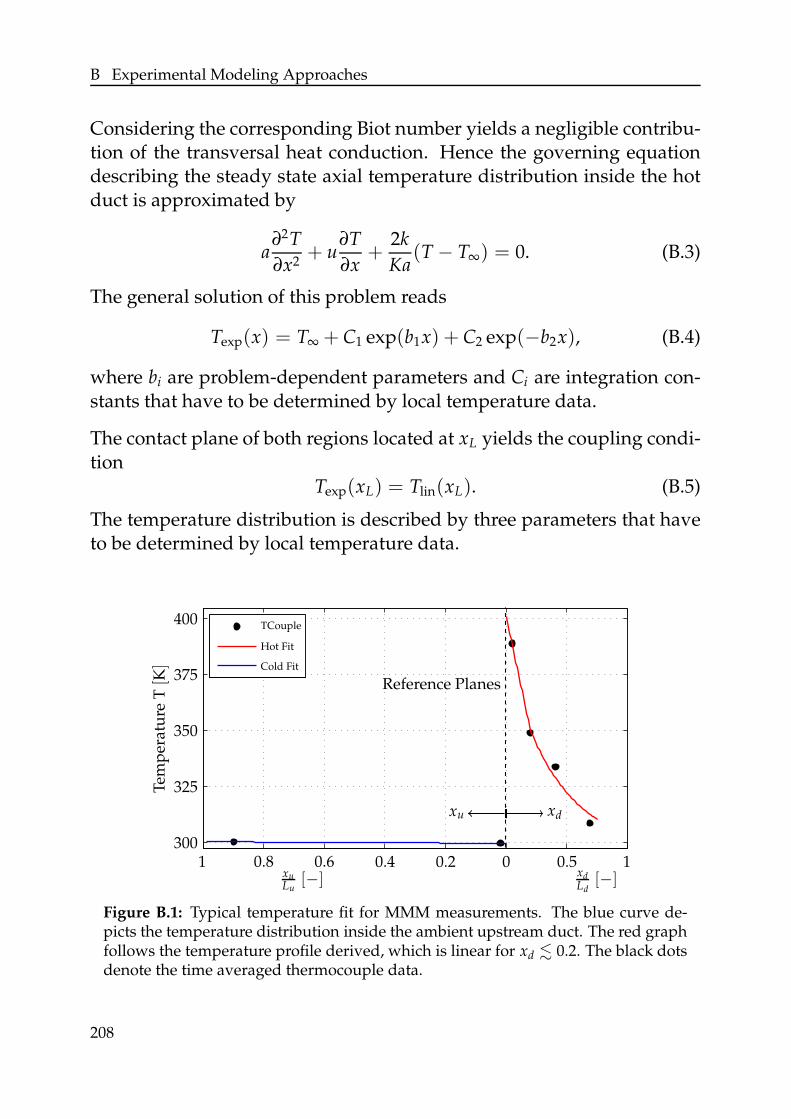
B Experimental Modeling Approaches
Considering the corresponding Biot number yields a negligible contribu-tion of the transversal heat conduction. Hence the governing equationdescribing the steady state axial temperature distribution inside the hotduct is approximated by
a∂2T
∂x2+ u
∂T
∂x+
2k
Ka(T − T∞) = 0. (B.3)
The general solution of this problem reads
Texp(x) = T∞ + C1 exp(b1x) + C2 exp(−b2x), (B.4)
where bi are problem-dependent parameters and Ci are integration con-stants that have to be determined by local temperature data.
The contact plane of both regions located at xL yields the coupling condi-tion
Texp(xL) = Tlin(xL). (B.5)
The temperature distribution is described by three parameters that haveto be determined by local temperature data.
0 11300
400
350
0.20.4 0.5
Tem
per
atu
reT[K]
0.8 0.6
325
375
TCouple
Hot Fit
Cold Fit
Reference Planes
xdxu
xuLu
[−] xdLd
[−]
Figure B.1: Typical temperature fit for MMM measurements. The blue curve de-picts the temperature distribution inside the ambient upstream duct. The red graphfollows the temperature profile derived, which is linear for xd . 0.2. The black dotsdenote the time averaged thermocouple data.
208
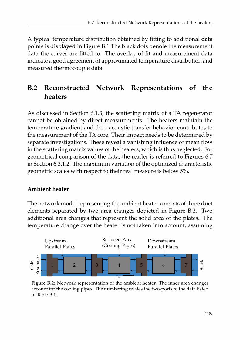
B.2 Reconstructed Network Representations of the heaters
A typical temperature distribution obtained by fitting to additional datapoints is displayed in Figure B.1 The black dots denote the measurementdata the curves are fitted to. The overlay of fit and measurement dataindicate a good agreement of approximated temperature distribution andmeasured thermocouple data.
B.2 Reconstructed Network Representations of the
heaters
As discussed in Section 6.1.3, the scattering matrix of a TA regeneratorcannot be obtained by direct measurements. The heaters maintain thetemperature gradient and their acoustic transfer behavior contributes tothe measurement of the TA core. Their impact needs to be determined byseparate investigations. These reveal a vanishing influence of mean flowin the scattering matrix values of the heaters, which is thus neglected. Forgeometrical comparison of the data, the reader is referred to Figures 6.7in Section 6.3.1.2. The maximum variation of the optimized characteristicgeometric scales with respect to their real measure is below 5%.
Ambient heater
The network model representing the ambient heater consists of three ductelements separated by two area changes depicted in Figure B.2. Twoadditional area changes that represent the solid area of the plates. Thetemperature change over the heater is not taken into account, assuming
1 2 3 4 5 6 7
xu
Co
ld
Res
on
ato
r
Sta
ck
UpstreamParallel Plates
Reduced Area(Cooling Pipes)
DownstreamParallel Plates
Figure B.2: Network representation of the ambient heater. The inner area changesaccount for the cooling pipes. The numbering relates the two-ports to the data listedin Table B.1.
209
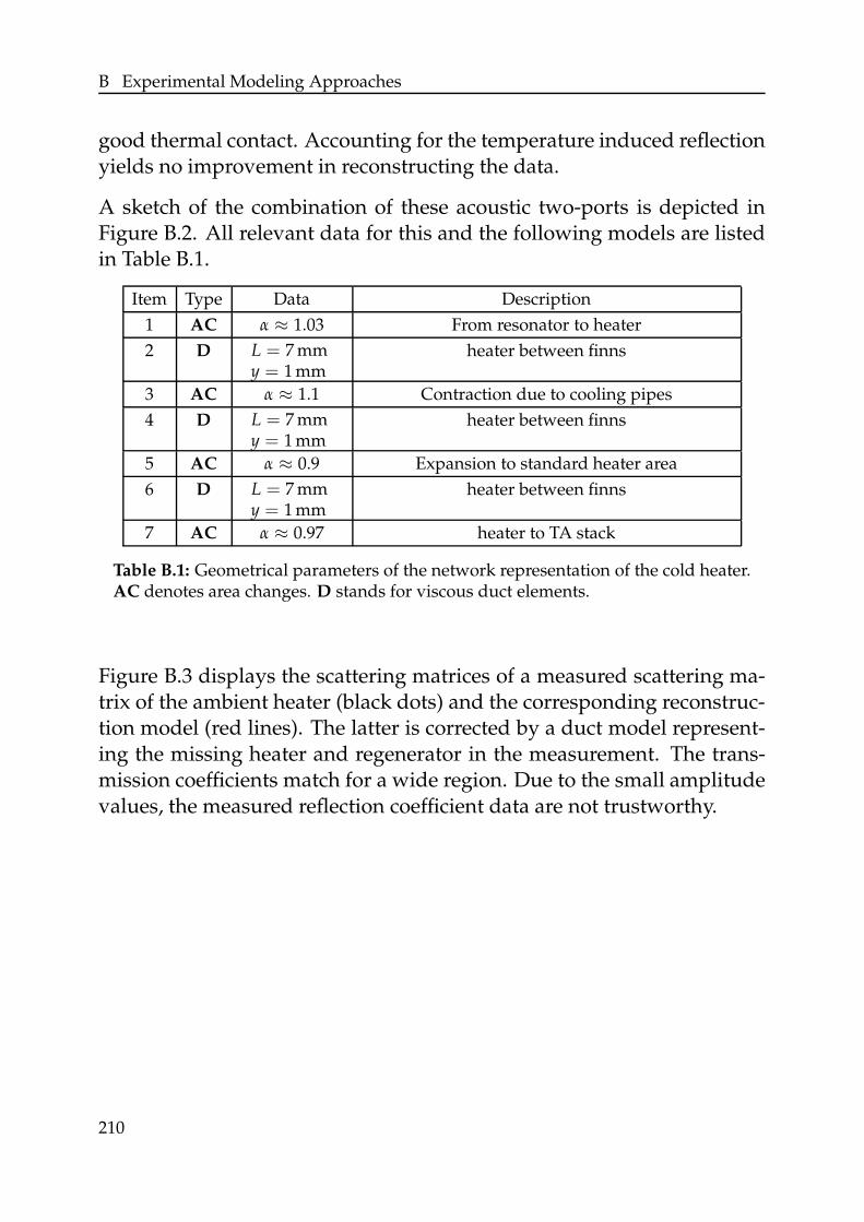
B Experimental Modeling Approaches
good thermal contact. Accounting for the temperature induced reflectionyields no improvement in reconstructing the data.
A sketch of the combination of these acoustic two-ports is depicted inFigure B.2. All relevant data for this and the following models are listedin Table B.1.
Item Type Data Description
1 AC α ≈ 1.03 From resonator to heater
2 D L = 7 mmy = 1 mm
heater between finns
3 AC α ≈ 1.1 Contraction due to cooling pipes
4 D L = 7 mmy = 1 mm
heater between finns
5 AC α ≈ 0.9 Expansion to standard heater area
6 D L = 7 mmy = 1 mm
heater between finns
7 AC α ≈ 0.97 heater to TA stack
Table B.1: Geometrical parameters of the network representation of the cold heater.AC denotes area changes. D stands for viscous duct elements.
Figure B.3 displays the scattering matrices of a measured scattering ma-trix of the ambient heater (black dots) and the corresponding reconstruc-tion model (red lines). The latter is corrected by a duct model represent-ing the missing heater and regenerator in the measurement. The trans-mission coefficients match for a wide region. Due to the small amplitudevalues, the measured reflection coefficient data are not trustworthy.
210
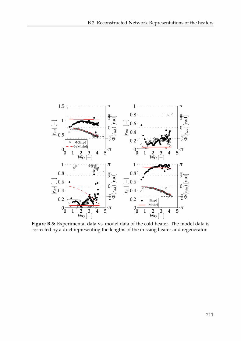
B.2 Reconstructed Network Representations of the heaters
00
00
00
00
00
00
11
11
1
1
1
1
1
1
1
1
22
22
22
22
33
33
33
33
44
44
44
44
55
55
55
55
0.20.2
0.2
0.40.4
0.40.5
0.60.6
0.6
0.80.8
0.8
1.5
Wo [−]Wo [−]
Wo [−]Wo [−]
|t ud|[−]
Φ(t
ud)[r
ad]
|t du|[−]
Φ(t
du)[r
ad]
|r dd|[−]
Φ(r
dd)[r
ad]
|r uu|[−]
Φ(r
uu)[r
ad]
ππ
ππ
π2
π2
π2
π2
00
00
-π2-π
2
-π2-π
2
-π-π
-π-π
|Model|
Φ(Model)
|Exp|
Φ(Exp)
Figure B.3: Experimental data vs. model data of the cold heater. The model data iscorrected by a duct representing the lengths of the missing heater and regenerator.
211
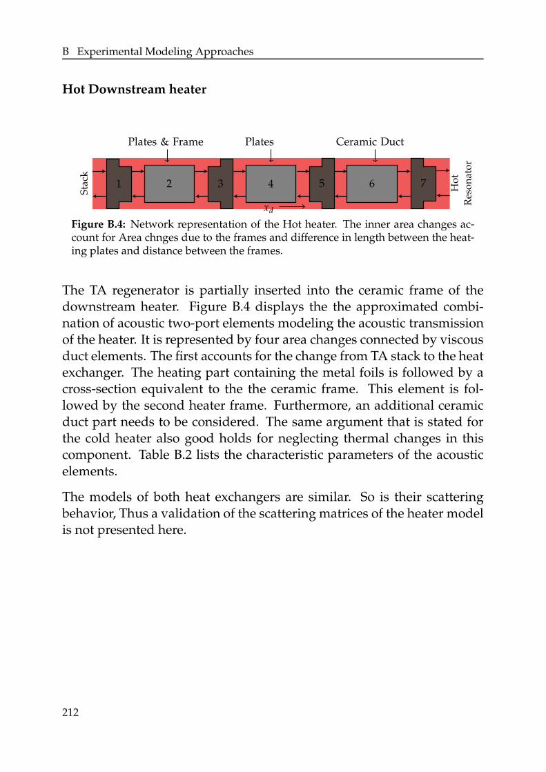
B Experimental Modeling Approaches
Hot Downstream heater
1 2 3 4 5 6 7
xd
Sta
ck
Ho
t
Res
on
ato
r
Plates & Frame Plates Ceramic Duct
Figure B.4: Network representation of the Hot heater. The inner area changes ac-count for Area chnges due to the frames and difference in length between the heat-ing plates and distance between the frames.
The TA regenerator is partially inserted into the ceramic frame of thedownstream heater. Figure B.4 displays the the approximated combi-nation of acoustic two-port elements modeling the acoustic transmissionof the heater. It is represented by four area changes connected by viscousduct elements. The first accounts for the change from TA stack to the heatexchanger. The heating part containing the metal foils is followed by across-section equivalent to the the ceramic frame. This element is fol-lowed by the second heater frame. Furthermore, an additional ceramicduct part needs to be considered. The same argument that is stated forthe cold heater also good holds for neglecting thermal changes in thiscomponent. Table B.2 lists the characteristic parameters of the acousticelements.
The models of both heat exchangers are similar. So is their scatteringbehavior, Thus a validation of the scattering matrices of the heater modelis not presented here.
212
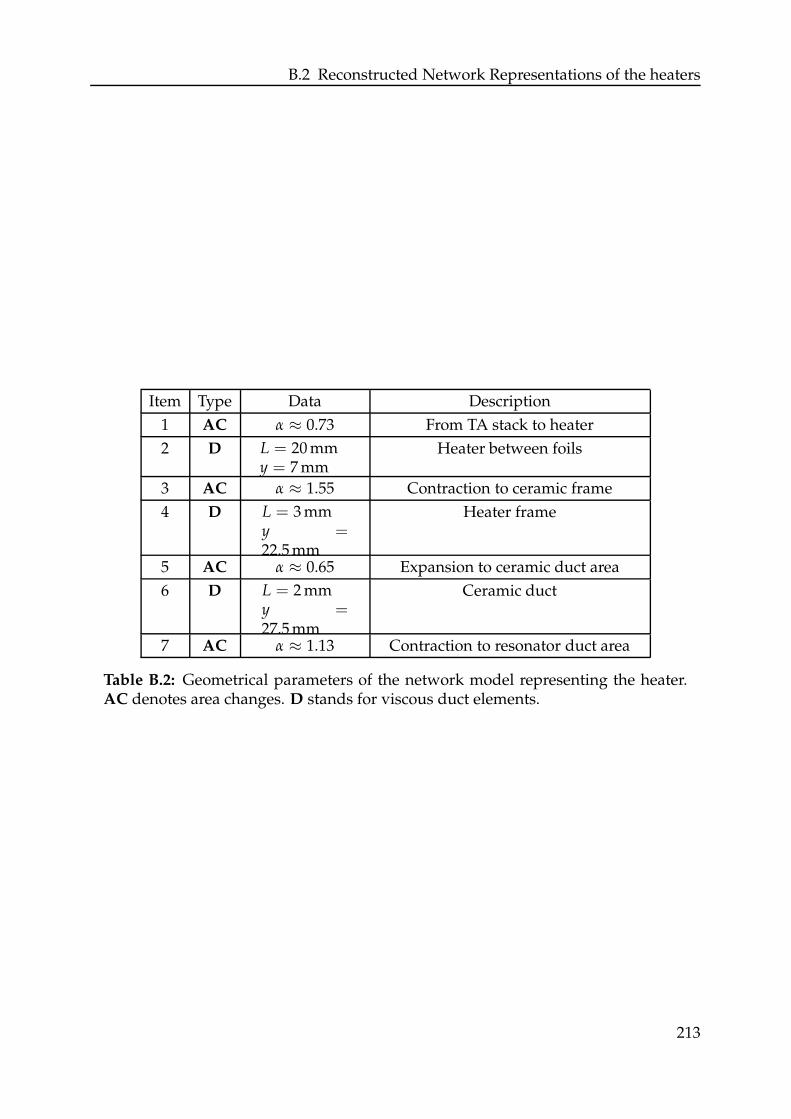
B.2 Reconstructed Network Representations of the heaters
Item Type Data Description
1 AC α ≈ 0.73 From TA stack to heater
2 D L = 20 mmy = 7 mm
Heater between foils
3 AC α ≈ 1.55 Contraction to ceramic frame
4 D L = 3 mmy =22.5 mm
Heater frame
5 AC α ≈ 0.65 Expansion to ceramic duct area
6 D L = 2 mmy =27.5 mm
Ceramic duct
7 AC α ≈ 1.13 Contraction to resonator duct area
Table B.2: Geometrical parameters of the network model representing the heater.AC denotes area changes. D stands for viscous duct elements.
213