Imperial College London

Department of Theoretical Physics

Aspects of Time in Quantum Theory

James M Yearsley

October 7, 2011

Submitted in part fulfilment of the requirements for the degree of

Doctor of Philosophy in Theoretical Physics of Imperial College London

and the Diploma of Imperial College London

1

Declaration

I herewith certify that all material in this dissertation which is not my own work has been

properly acknowledged.

James M Yearsley

2

Abstract

We consider a number of aspects of the problem of defining time observables in quantum

theory. Time observables are interesting quantities in quantum theory because they of-

ten cannot be associated with self-adjoint operators. Their definition therefore touches on

foundational issues in quantum theory.

Various operational approached to defining time observables have been proposed in the

past. Two of the most common are those based on pulsed measurements in the form of strings

of projection operators and continuous measurements in the form of complex potentials. One

of the major achievements of this thesis is to prove that these two operational approaches

are equivalent.

However operational approaches are somewhat unsatisfying by themselves. To provide a

definition of time observables which is not linked to a particular measurement scheme we

employ the decoherent, or consistent, histories approach to quantum theory. We focus on the

arrival time, one particular example of a time observable, and we use the relationship between

pulsed and continuous measurements to relate the decoherent histories approach to one based

on complex potentials. This lets us compute the arrival time probability distribution in

decoherent histories and we show that it agrees with semiclassical expectations in the right

limit. We do this both for a free particle and for a particle coupled to an environment.

Finally, we consider how the results discussed in this thesis relate to those derived by

coupling a particle to a model clock. We show that for a general class of clock models the

probabilities thus measured can be simply related to the ideal ones computed via decoherent

histories.

3

For my parents, to whom I owe everything

and

For Laura, whose love and support made this possible.

but more than all(as all your more than eyes

tell me)there is a time for timelessness

E.E. Cummings

4

Preface

The work presented in this thesis was carried out in the Theoretical Physics Group, Imperial

College, between October 2007 and September 2011. The supervisor was Prof. Jonathan J.

Halliwell.

The results presented in Chapters 3 and 7 were published in Journal of Physics A [99]

and Physical Review A [100] respectively. The work presented in Chapter 4 was done in

collaboration with Jonathan Halliwell and published in Journal of Physics A [51]. Chapters

5 and 6 are based on work done in collaboration with Jonathan Halliwell and published in

Physical Review A [49] and Physics Letters A [50]. The work presented in Chapter 8 was

done in collaboration with Delius Downs, Jonathan Halliwell and Anna Hashagen and was

published in Physical Review A [101].

I am grateful to Carl Bender, Adolfo del Campo, Fay Dowker, Bei-Lok Hu, Seth Lloyd,

Gonzalo Muga, Lawrence Schulman and Antony Valentini for their comments and sugges-

tions on the material contained in this thesis.

Some of the work in this thesis was carried out during a short stay at the Apuan Alps

Centre for Physics at the Towler Institute, Italy during the conference “21st Century direc-

tions in de Broglie-Bohm theory and beyond.” I would like to thank Mike Towler and the

other conference organisers for their hospitality.

In addition I would like to thank Kate Clements, Ben Hoare, Steven Johnston, Sam

Kitchen, Johannes Knoller, Noppadol ‘Omega’ Mekareeya, Tom Pugh and David Weir for

many useful, informative and occasionally even relevant discussions.

None of the work set out in this thesis would have been possible without the limitless

support and encouragement of my supervisor, Jonathan Halliwell. I am grateful for all his

help over the four years of my PhD here at Imperial and I consider myself incredibly fortunate

to have had him as a teacher and collaborator.

5

Contents

Abstract 3

Preface 5

1 Introduction 10

1.1 A Brief History of Time in Quantum Theory . . . . . . . . . . . . . . . . . . 10

1.2 The Quantum Zeno Effect . . . . . . . . . . . . . . . . . . . . . . . . . . . . 15

1.3 The Backflow Effect . . . . . . . . . . . . . . . . . . . . . . . . . . . . . . . 18

1.4 The Arrival Time Problem in Quantum Mechanics . . . . . . . . . . . . . . . 19

1.4.1 General Theory . . . . . . . . . . . . . . . . . . . . . . . . . . . . . . 19

1.4.2 Standard Forms of the Arrival Time Distribution . . . . . . . . . . . 21

1.5 The Decoherent Histories Approach to Quantum Theory . . . . . . . . . . . 24

1.6 The Decoherent Histories Approach to the Arrival Time Problem: Introduc-

tion and History . . . . . . . . . . . . . . . . . . . . . . . . . . . . . . . . . . 27

1.7 Summary and Overview of the Rest of This Thesis . . . . . . . . . . . . . . 29

2 The Path Decomposition Expansion (PDX) 32

2.1 Introduction . . . . . . . . . . . . . . . . . . . . . . . . . . . . . . . . . . . . 32

2.2 The Path Decomposition Expansion (PDX) . . . . . . . . . . . . . . . . . . 32

2.3 Using the PDX: Scattering States for a Complex Step Potential . . . . . . . 35

2.4 A Semiclassical Approximation . . . . . . . . . . . . . . . . . . . . . . . . . 37

3 The Propagator for the Step and Delta Function Potentials, using the

PDX 40

3.1 Introduction . . . . . . . . . . . . . . . . . . . . . . . . . . . . . . . . . . . . 40

3.2 The Brownian Motion Definition of the Propagator . . . . . . . . . . . . . . 41

3.3 The Step Potential . . . . . . . . . . . . . . . . . . . . . . . . . . . . . . . . 42

3.4 The Delta Function Potential . . . . . . . . . . . . . . . . . . . . . . . . . . 45

4 On the Relationship between Complex Potentials and Strings of Projection

Operators 48

6

4.1 Introduction . . . . . . . . . . . . . . . . . . . . . . . . . . . . . . . . . . . . 48

4.2 Review and Extension of Earlier Work . . . . . . . . . . . . . . . . . . . . . 51

4.3 Detailed Formulation of the Problem . . . . . . . . . . . . . . . . . . . . . . 52

4.4 Exact Analytic Results . . . . . . . . . . . . . . . . . . . . . . . . . . . . . . 59

4.5 Asymptotic Limit . . . . . . . . . . . . . . . . . . . . . . . . . . . . . . . . . 63

4.6 A Time Averaged Result . . . . . . . . . . . . . . . . . . . . . . . . . . . . . 64

4.7 Numerical Results . . . . . . . . . . . . . . . . . . . . . . . . . . . . . . . . . 66

4.8 Timescales . . . . . . . . . . . . . . . . . . . . . . . . . . . . . . . . . . . . . 70

4.9 Summary and Discussion . . . . . . . . . . . . . . . . . . . . . . . . . . . . . 71

5 Arrival Times, Complex Potentials and Decoherent Histories 74

5.1 Introduction . . . . . . . . . . . . . . . . . . . . . . . . . . . . . . . . . . . . 74

5.2 The Classical Arrival Time Problem via a Complex Potential . . . . . . . . . 76

5.3 Calculation of the Arrival Time Distribution via a Complex Potential . . . . 79

5.4 Decoherent Histories Analysis for a Single Large Time Interval . . . . . . . . 83

5.5 Decoherent Histories Analysis for an Arbitrary Set of Time Intervals . . . . . 86

5.5.1 Class Operators . . . . . . . . . . . . . . . . . . . . . . . . . . . . . . 86

5.5.2 An Important Simplification of the Class Operator . . . . . . . . . . 88

5.5.3 Probabilities for Crossing . . . . . . . . . . . . . . . . . . . . . . . . . 89

5.5.4 Decoherence of Histories and the Backflow Problem . . . . . . . . . . 89

5.5.5 The Decoherence Conditions . . . . . . . . . . . . . . . . . . . . . . . 90

5.5.6 Checking the Decoherence Condition for Wavepackets . . . . . . . . . 91

5.6 Summary and Conclusions . . . . . . . . . . . . . . . . . . . . . . . . . . . . 96

6 Arrival Times, Crossing Times and a Semiclassical Approximation 98

6.1 Introduction . . . . . . . . . . . . . . . . . . . . . . . . . . . . . . . . . . . . 98

6.2 Semiclassical Derivation of the Arrival Time Class Operators . . . . . . . . . 101

6.3 Arrival Times, Crossing Times and First Crossing Times . . . . . . . . . . . 103

6.4 Crossing Class Operators in Decoherent Histories . . . . . . . . . . . . . . . 105

6.5 Crossing Time Probabilities and Decoherence of Crossing Histories . . . . . . 107

6.6 Summary and Discussion . . . . . . . . . . . . . . . . . . . . . . . . . . . . . 109

7 Quantum Arrival Time for Open Systems 110

7.1 Introduction . . . . . . . . . . . . . . . . . . . . . . . . . . . . . . . . . . . . 110

7.2 Arrival Time for Open Quantum Systems . . . . . . . . . . . . . . . . . . . . 113

7.3 Quantum Brownian Motion . . . . . . . . . . . . . . . . . . . . . . . . . . . 116

7.4 Properties of the Arrival Time Distribution in Quantum Brownian Motion . 118

7.5 The Decoherent Histories Approach to the Arrival Time Problem . . . . . . 122

7

7.6 Decoherence of Arrival Times in Quantum Brownian Motion . . . . . . . . . 125

7.6.1 General Case . . . . . . . . . . . . . . . . . . . . . . . . . . . . . . . 125

7.6.2 The Near-Deterministic Limit . . . . . . . . . . . . . . . . . . . . . . 128

7.7 Summary and Discussion . . . . . . . . . . . . . . . . . . . . . . . . . . . . . 132

8 Quantum Arrival and Dwell Times via an Ideal Clock 135

8.1 Introduction . . . . . . . . . . . . . . . . . . . . . . . . . . . . . . . . . . . . 135

8.1.1 Opening Remarks . . . . . . . . . . . . . . . . . . . . . . . . . . . . . 135

8.1.2 Dwell Time . . . . . . . . . . . . . . . . . . . . . . . . . . . . . . . . 135

8.1.3 Clock Model . . . . . . . . . . . . . . . . . . . . . . . . . . . . . . . . 136

8.1.4 Connections to Earlier Work . . . . . . . . . . . . . . . . . . . . . . . 138

8.1.5 This Chapter . . . . . . . . . . . . . . . . . . . . . . . . . . . . . . . 138

8.2 Arrival Time Distribution from an Idealised Clock . . . . . . . . . . . . . . . 138

8.2.1 Weak Coupling Regime . . . . . . . . . . . . . . . . . . . . . . . . . . 139

8.2.2 Strong Coupling Regime . . . . . . . . . . . . . . . . . . . . . . . . . 141

8.3 Dwell Time Distribution from an Idealised Clock . . . . . . . . . . . . . . . . 144

8.4 Conclusion . . . . . . . . . . . . . . . . . . . . . . . . . . . . . . . . . . . . . 147

9 Summary and Some Open Questions 148

9.1 Summary . . . . . . . . . . . . . . . . . . . . . . . . . . . . . . . . . . . . . 148

9.2 Open Questions and Future Work . . . . . . . . . . . . . . . . . . . . . . . . 149

Appendix: Some Properties of the Current 151

8

List of Figures

1.1 Probabilities for Space-like and Time-like Surfaces . . . . . . . . . . . . . . . 12

1.2 The Arrival Time Problem . . . . . . . . . . . . . . . . . . . . . . . . . . . . 19

2.1 The Path Decomposition Expansion (PDX) . . . . . . . . . . . . . . . . . . 34

3.1 A Typical Path From x = 0 to x = 0 On Our Lattice. . . . . . . . . . . . . . 43

3.2 The Bijection Between n(k) and Cn. . . . . . . . . . . . . . . . . . . . . . . 44

4.1 The Path Decomposition Expansion for gP . . . . . . . . . . . . . . . . . . . . 55

4.2 A Plot Comparing the Functions fV (t) and fP (t). . . . . . . . . . . . . . . . 58

4.3 Plot of the Exact Value of fP (t) Compared With an Analytic Approximation. 68

4.4 A Plot of the Function S(t). . . . . . . . . . . . . . . . . . . . . . . . . . . . 69

5.1 Recap of the Arrival Time Problem. . . . . . . . . . . . . . . . . . . . . . . . 74

5.2 Plot of the Function f(u). . . . . . . . . . . . . . . . . . . . . . . . . . . . . 93

5.3 The Arrival Time of a Superposition of Two Wavepackets. . . . . . . . . . . 96

6.1 Crossing Times . . . . . . . . . . . . . . . . . . . . . . . . . . . . . . . . . . 99

6.2 Crossing Times and First Crossing Times . . . . . . . . . . . . . . . . . . . . 104

7.1 Arrival Times in Terms of Initial States and Propagators. . . . . . . . . . . . 128

8.1 The Arrival Time Problem Defined Using a Model Clock. . . . . . . . . . . . 137

8.2 The Dwell Time Problem, Defined Using a Model Clock. . . . . . . . . . . . 144

8.3 The PDX Used for the Dwell Time Problem. . . . . . . . . . . . . . . . . . . 145

9

1 Introduction

The time is out of joint; O cursed sprite,

That ever I was born to set it right!

Shakespeare, Hamlet

1.1 A Brief History of Time in Quantum Theory

The treatment of time observables is an important loose end in quantum theory [81, 80].

Whilst there is no indication of any disagreement between the predictions of quantum theory

and the outcomes of experiment, time observables constitute a class of quantities that are

observables in classical mechanics, but for which no satisfactory treatment exists in standard

quantum theory.

As well as being an important topic in its own right, a consistent treatment of time

observables might also shed light on problems in quantum gravity and quantum cosmology.

One of the most tricky problems faced by any attempt to quantise gravity is that of the

problem of time [64]. In essence the symmetries of general relativity prevent the identification

of any variable to play the role of time in quantum gravity. Whilst there is no generally agreed

way of tackling this problem one school of thought holds that any approach to quantising

gravity must proceed by treating time and space on an equal footing. A theory treating time

and space in a truly symmetric way would have as observables probabilities for entering given

regions of spacetime rather than, for example, statements about the position of a particle

at a fixed moment of time. Since these are not the kind of probabilities one normally deals

with in quantum theory it is instructive to see if the same exercise can be performed in

non-relativistic quantum theory. That is, can one assign probabilities to questions of the

form, “What is the probability of finding a particle in a given region of space, ∆, in a given

interval of time, [t0, t1]?”

Asking questions of this sort quickly leads us to another problem in non-relativistic quan-

tum theory, which is this: “What exactly is the status of the variable t that appears in

Schrodinger’s equation?” It should be clear immediately that it is not related to any oper-

ator on the Hilbert space of the system. Indeed it is not really a quantum quantity at all

10

and is probably best thought of as referring to some external classical clock. This hybrid

approach to dynamics, having a quantum wavefunction depend on an external classical clock

variable, could be seen as troubling. An operationalist might reply that the co-ordinate x

also refers to an external classical world, but this line of reasoning is over simplistic for three

reasons. The first is that both position and its conjugate variable, momentum, appear as

operators in quantum mechanics, whereas energy is represented by an operator in quantum

mechanics, but time is not. There is therefore a lack of symmetry in the treatment. The

second reason is that quantum mechanics may be written in a representation-free manner

in terms of abstract vectors in Hilbert space. Here there need be no mention of position

or momentum, and yet the Schrodinger equation for evolution in this abstract space still

includes the time coordinate. The final reason is the most profound, and again touches on

the lack of symmetry in the treatment of space and time coordinates. In non-relativistic

quantum mechanics, the object,

P (x)dx = |ψ(x, t)|2dx (1.1)

gives the probability of finding the particle in the interval [x, x + dx] at the time t. What

is the corresponding probability for finding the particle at the position x in the interval

[t, t+ dt]? It is not given by

P (t)dt 6= |ψ(x, t)|2dt, (1.2)

since finding the particle at a position x at the times t1 or t2 are not exclusive alternatives,

see Fig.(1.1). Yet in the standard interpretations of quantum mechanics the wavefunction is

supposed to contain all the information about a given system [67]. If the square norm of a

general wavefunction is not a probability distribution on a set of times does this mean there

can be no satisfactory treatment of time observables in standard quantum theory?

To get a better idea of where the difficulty lies it is instructive to look more closely at the

classical case. Here the solution of a particular problem may be expressed in terms of an

equation of motion for the particle, of the form,

x = f(t, x0, p0) (1.3)

where x0 represents the initial condition. This is the solution to the question: “Where is

the particle at time t?” Under general conditions one may invert this equation of motion to

give,

t = F (x, x0, p0) (1.4)

which is the solution to the question: “When is the particle at position x?” Crucial to this

analysis is the concept of a trajectory and that the particle will with certainty be found

11

x

t

A B

(a) Probabilities for Space-like Surfacesx

t

A

B

(b) Probabilities for Time-like Surfaces

Figure 1.1: (a) Since every trajectory crosses a surface of constant time only once, passingthrough disjoint intervals A or B at a given time represent exclusive alternatives. (b) Incontrast trajectories may cross a surface of constant position many times. Therefore passingthrough disjoint intervals A or B are not exclusive alternatives.

somewhere on this trajectory, at any time. This concept is of course lacking in quantum

theory.

In classical mechanics observables are given by functions on phase space, and so Eq.(1.4)

is equivalent to some phase space function,

t = τ(x, p). (1.5)

Crucially, unlike classical observables like the energy or angular momentum, construction

of Eq.(1.5) requires knowledge of the equations of motion, Eq.(1.3). Strictly speaking then,

even in classical mechanics questions such as “When does the particle reach the origin?” have

a different character to questions like “What is the energy of the particle?”. The observable

coresponding to the former is a function on phase space which is constructed using the

equations of motion. In a sense, therefore, the surprise is not that quantum theory struggles

to deal with time observables, but that classical mechanics deals with them so easily. This

is essentially a consequence of the realist nature of classical physics.

Approaches to the problem of defining time observables in quantum theory fall roughly into

three camps. Although it is not the intention of this thesis to provide a complete overview

of the literature on time observables (see Ref.[77] for a detailed review in the case of arrival

12

time), the following characterisations will be useful in understanding how the approaches

taken in this work relate to previous studies.

Trajectory Before Quantisation

These are approaches which in some way borrow the classical structure of a trajectory and

use it in the quantum analysis. One way to do this is to begin with the classical description,

in terms of Eq.(1.3) and use this to construct the classical phase space observable Eq.(1.5),

as outlined above. One then tries to quantise this quantity to obtain the operator,

t = τ(x, p) (1.6)

This category of approaches includes the Aharanov-Bohm time operator [3]. Apart from the

obvious issues surrounding whether Eq.(1.6) is well defined for a given classical observable,

there is something troubling about this analysis. Since the quantum system we are trying to

analyse will not be explicable in terms a particle following a single trajectory, it is not clear

whether using the classical trajectory to obtain the operator Eq.(1.6) is a valid procedure.

Even if the resulting operator is well defined the relation between this observable and the

results of measurement remains unclear. Since this is essentially the question of how to un-

derstand the quantisation of a given classical system we are unlikely to make much headway

with this issue here. It does, however, motivate trying to find an alternative way to proceed.

Other approaches that fall into this category include the analysis of Kijowski and its vari-

ants, see eg Refs.[68, 61]. Here one begins by deciding what properties one would expect

the quantum probability distribution to possess, such as time translation covariance or pos-

itivity, based on the properties of the classical observable. One then uses this “wish list”

of properties to determine the correct operator, with the eventual hope that a sufficiently

detailed list of properties might uniquely determine this operator. It is not clear that this

approach should work in all cases however: it is easy to think of quantum observables, such

as angular momentum or the energy levels of a harmonic oscillator, that have a very different

character from their classical counterparts.

The general attitude of this thesis is that whilst any of the analyses above might arrive at

the correct definition of a time observable in a particular case, they cannot be relied upon

to do so in all cases.

Trajectory After Quantisation

These approaches include those based on the de Broglie-Bohm (dBB) interpretation of quan-

tum theory [63], analyses based on the WKB approximation [40] and also the decoherent

13

histories approach presented in this thesis. Here one first quantizes the system and then

looks for structures to play the role of the classical trajectories used to define the classical

observables. For example for gaussian states the center of the wavepacket will follow simple

curve in configuration space. Provided one does not perform measurements that disturb this

state this limited notion of trajectory can be used to find approximate arrival and dwell times

for the particle, limited by the width of the wavepacket. Of course these states form only a

limited class of possible states, and it is a general feature of this category of approaches that

they may fail for highly non-classical states.

In the DH approach, described in more detail below, the aim is to assign probabilities to

coarse grained histories of a quantum system. Provided these probabilities can be assigned

consistently one can then use these histories in much the same way as the classical trajectories

to discus time observables.

In the dBB interpretation, the wavefunction is supplemented by a real particle follow-

ing a trajectory computed from the wavefunction. Since a quantum particle always comes

equipped with a unique trajectory computation of time observables is, at least conceptually,

as trivial as in the classical case. The price one pays, however, is that the behavior of these

trajectories generally depends on whether or not one choses to carry out a measurement on

the system. Thus although in dBB probabilities for time observables can be obtained with-

out the need for an observer, the probabilities obtained in this way do depend on whether

or not there is an observer. We will not have much to say in this thesis about dBB, for more

information see Ref.[63].

Trajectory Free Approaches

These approaches may also be called “operational.” Here one takes a completely different

tack and instead looks for other ways to define time observables classically, and then tries

to repeat this analysis quantum mechanically.

These approaches include studies based on model clocks, see Ref.[88] and Chapter 8 of this

thesis. Here the idea is to couple the system we wish to measure to some additional degrees

of freedom which function as a clock. In this context a clock is simply a quantum system

coupled to our system of interest in such a way that the final state of the clock is correlated

with the time observable we wish to measure. More details about this scheme can be found

in Chapter 8.

In classical mechanics many time observables can be defined by imposing absorbing bound-

ary conditions on the system. See Chapter 5 for a full discussion in the arrival time case.

The analogue of these absorbing boundary conditions in quantum theory in the inclusion of

a complex absorbing potential, see Ref.[76] and also Chapter 5 of this thesis.

14

Typically the probability distributions obtained from these approaches are complicated

functions of the properties of both the particle and measuring apparatus. There may or may

not exist limits in which dependence on the measurement parameters drops out, depending

on the set up.

As well as the technical differences between these approaches the different approaches

display very different attitudes towards the observables we are trying to define. In particular

the first and third approaches assume that an observable such as the arrival time of a particle

is always a well defined quantity and that for any system one may obtain the probability

distribution of that observable. The second class of approaches, in contrast, are based on

recovering the classical notion of trajectory after quantisation, and thus they are generally

only well defined for semiclassical systems. Proponents of these approaches would claim

that quantities such as the arrival time distribution are only defined for suitably classical

systems1.

An obvious question is whether there is anything linking these three different approaches

to time observables. This is an important question, firstly since although any particular

approach might claim to have the solution to these problems the validity of these approaches

themselves is questionable. If we could demonstrate that for a particular time observable

the same results are obtained via a number of approaches this would give us confidence that

this result is correct. Secondly, the different approaches discussed above have their roots in

different interpretations of quantum theory. Although we will try and avoid philosophical

questions about the foundations of quantum theory in this thesis if we were to show that,

for example, expressions for time observables in de Broglie-Bohm theory were identical to

those obtained via decoherent histories this might shed interesting light on the relationship

between different interpretations of quantum theory 2.

1.2 The Quantum Zeno Effect

There are a number of interesting quantum effects relevant to the definition of time observ-

ables, the most important of which is probably the quantum Zeno effect. The effect was first

noticed by Allcock in his seminar series of papers on the arrival time problem [6], but the

1In much the same way as it is claimed that time itself is only emergent, from an ultimately timeless theoryof quantum gravity [13].

2Not to mention the fact that although any interpretation of quantum theory is constrained by the require-ment that it must agree with the predictions of standard Copenhagen quantum theory, since Copenhagenquantum theory struggles to incorporate many time observables there is a possibility that different inter-pretations of quantum theory may be free to make different predictions for time observables. There maytherefore be experimental tests that could be done to distinguish between them. Exciting as this line ofthought is, we shall not dwell on it in this thesis.

15

first serious study was undertaken by Misra and Sudershan in Ref.[74].

The quantum Zeno effect is often expressed as a “freezing” of evolution due to repeated

measurement. Much has been learned about the phenomenon since the early investigations

however and it is now understood that there is more to the effect than simply preventing

evolution. Repeated projections onto a subspace allow for unitary evolution within that

subspace, the effect of the repeated measurement being simply equivalent to imposing “hard-

wall” boundary conditions, preventing the particle from leaving the subspace [27]. It is also

known that there also exists an “anti-Zeno” effect, that is, a speeding up of evolution due

to repeated measurement [26], although we shall have nothing to say about the anti-Zeno

effect in this thesis.

The quantum Zeno effect plays an important role in study of time observables because,

at least for the “trajectory after quantisation” and “trajectory free” approaches outlined in

the previous section, the definition of these observables involves statements about the state

of the system at multiple times. This means one has to consider sequential measurements

on the system of interest, if these are performed too frequently the quantum Zeno effect

will result. However the situation is complicated by the fact that most discussions of the

quantum Zeno effect take place in a setting appropriate for quantum optics or quantum

information, ie a system with a small number of discrete energy levels, not in the context

of particles in 1D. In the rest of this section we therefore outline the standard discussion of

the quantum Zeno effect and the way in which this discussion might be modified to make it

relevant to time observables. Our discussion will be brief, since the details of the Zeno limit

in the arrival time problem etc are worked out more thoroughly in Chapter 4.

We begin by introducing the Zeno effect in the way it appears in the original discussion of

Misra and Sudarshan, Ref.[74]. The idea is to utilise some form of product formula to show

that the repeated process of evolution followed by measurement is equivalent to restricted

evolution in the subspace defined by the measurement. We consider a system with initial

state |ψ〉 which evolves under a Hamiltonian H for a total time T , interspersed with N

projective measurements P . The state at time T is given by,

|ψT 〉 = VN(T ) |ψ〉 = e−iHT/NPe−iHT/N ...e−iHT/NP |ψ〉= [exp(−iHT/N)P ]N |ψ〉 (1.7)

One then considers the limit N →∞, and one can show, under certain conditions on H and

P ,

V∞(T ) = limN→∞

VN(T ) = exp(−iHZT )P, (1.8)

where the Zeno hamiltonian HZ = PHP . This shows that evolution under repeated mea-

16

surement leads to unitary evolution in the subspace defined by the measurements.

If we consider the evolution in Eq.(1.7), with P = θ(x) and H the free hamiltonian for

a particle in 1D, we have a simple model of the type of measurement set up we might use

to determine the time at which the particle arrived at x = 0. Without concerning ourselves

too much with the details, since these are covered in Section 1.4 and the rest of this thesis,

it is clear that the Zeno effect sets a lower limit on the resolution with which we can define

an arrival time using this set up.

Although this analysis is mathematically precise this precision is obtained at the expense

of providing any great physical insight. A key question concerns the time scale on which the

Zeno effect begins to occur. That is, what is the minimum spacing between measurements,

T/N , that I can take without causing significant reflection from the measuring aparatus.

This is important since we can hardly expect to achieve N →∞ in the real word. One way

to approach this is to look for the time scale on which the state may be said to leave the

subspace defined by P . The idea is that projections more frequent than this will “interrupt”

the state in the process of exiting the region, so that this time scale provides an upper bound

on the separation between projections necessary to give rise to the Zeno effect. We follow

the analysis of Peres [87] and consider an initial state, with evolution for a time t followed by

a measurement which projects back onto the original state. The survival probability, S(t),

is given by,

S(t) = || 〈ψ| exp(−iHt) |ψ〉 ||2= 1− t2(∆H)2 +O(t4) = 1− (t/τz)

2 +O(t4) (1.9)

where we have defined the “Zeno time”3,

τ−2z = (∆H)2 = 〈ψ|H2 |ψ〉 − 〈ψ|H |ψ〉2 . (1.10)

We see from this expression that the short time behaviour is quadratic in t, thus we confirm

that in the limit of infinitely frequent measurements the state does not evolve. Secondly,

we see that there is a characteristic time scale, τZ = (∆H)−1, on which the evolution takes

place.

Although we have arrived here at what is normally called the “Zeno” time, it is not clear

that this really is the time scale on which the projections give rise to reflection and thus the

Zeno effect. For a minimum uncertainty gaussian wavepacket with spatial width σ peaked

around some momentum p0 Eq.(1.10) gives τz = mσ/|p0|. This is indeed the time scale on

3Note that there are many different notions of the time it takes a system to make a transition. See [92] fora more detailed discussion.

17

which the state crosses the origin, however this is an essentially classical timescale and it

seems unlikely that this is relevant for reflection, which is a quantum effect. It is also worth

pointing out that if we really are limited in the accuracy of our description by the time

scale 1/∆H then it is impossible to formulate a description of crossing time probabilities in

the normal sense. This is because our minimum temporal resolution is the same order as

the time taken for our wavepacket to cross the origin, so the probabilities for crossing will

essentially be 1 for one time interval and 0 for the rest.

Projecting back onto the original state captures the notion of the time on which the state

changes, and this is certainly the same as leaving some subspace of the full Hilbert space, but

we are interested in a particular subspace, that of states with support only in x > 0 and this

analysis does not capture that. There is another problem, which is that Eq.(1.9) is a Taylor

expansion of the initial state about t = 0. It is known that for general wavefunctions the

behaviour may not be analytic at t = 0. Put another way, the Zeno time is expressed in terms

of moments of the wavefunction, and these may not exist for general wavefunctions. This is

particularly apparent when one tries to extend this analysis to more general measurements.

One of the major achievements in this thesis is to show, in Chapter 4, that the minimum

temporal resolution is in fact set by 1/E, where E is the energy of the system, and not by

Eq.(1.10).

1.3 The Backflow Effect

Another quantum effect relevant to the understanding of time observables is the backflow

effect [12, 25]. Consider an initial state |ψ〉 consisting entirely of negative momenta evolved

freely for a time t and compute the standard Schrodinger probability current at the origin,

defined in such a way that classically it should be positive. This can be written in operator

form as,

J(t) =(−1)

2m〈ψ| eiHt{pδ(x) + δ(x)p}e−iHt |ψ〉 . (1.11)

(We will discuss the current in much more detail in later sections.) Now the operator

(−)(pδ(x) + δ(x)p) is not positive, even when restricted to act on states with negative mo-

mentum. This means although Eq.(1.11) should be positive classically, it need not be quan-

tum mechanically. What is remarkable is that very little is known about this effect. One

thing that is known is that the amount of probability that can flow backwards is bounded,

in the sense that, ∫ t2

t1

dtJ(t) ≥ λ, (1.12)

18

where λ is some dimensionless constant computed numerically to be λ ≈ −0.0384517 [25].

The existence of such a bound is somewhat unexpected, Bracken and Melloy in Ref.[12] con-

jecture that it is a “new dimensionless quantum number.” Certainly there is no dependence

on h in this constant and as such it has no obvious classical limit.

One interesting set of questions concern the state for which this bound is obtained, does

it have an analytical expression? Does it have an obvious physical interpretation? Another

question concerns the typicality, or otherwise, of backflow. Do relatively standard wavefunc-

tions such as gaussian wavepackets or superpositions of these give backflow, or do we require

more pathalogical states? If we can indeed produce backflow with more familiar states, is it

possible to get close to the maximum amount of backflow?

Some work towards addressing these questions is in progress [102], but much remains

unclear. A better understanding of the backflow effect would shed much light on the problem

of defining time observables in quantum theory. This is because, together with the Zeno

effect, it is these quantum effects that provide the fundamental limitation on the accuracy

with which time observables can be defined.

1.4 The Arrival Time Problem in Quantum Mechanics

1.4.1 General Theory

t1

x

t2

t

t=0

Figure 1.2: The Arrival Time Problem: What is the probability that an incoming wavepacketcrosses the origin during the time interval [t1, t2]?

Much of this thesis will be concerned, directly or otherwise, with the question of analysing

19

the arrival time problem in quantum theory, pictured in Fig.(1.2). It therefore seems useful

to give a brief account of the problem here and also discuss some of the features any solution

must posses.

The classical “arrival time problem” is the following, “Given a free particle which, at t = 0

has position q0 and momentum p0, what is the time at which the particle crosses the origin?”

The solution, of course, is that the particle crosses at a time,

τc = −mq0

p0

. (1.13)

In order to compare the definition of time observables in classical and quantum physics it is

useful to work in terms of classical phase space distributions. For a free classical particle in

1D the phase space probability distribution wt(q, p) obeys the following,

∂w

∂t= − p

m

∂w

∂q. (1.14)

The solutions of this equation are of the form,

wτ (q, p) = w0(q − pτ/m, p), (1.15)

so that evolution is just a linear transformation in phase space.

We can write the probability of crossing at a time τ in terms of this distribution as,

Πc(τ) =

∫dpdqδ(τ +mq/p)w0(q, p) =

∫dpdq

|p|δ(q)m

wτ (q, p) (1.16)

For states consisting of entirely negative momenta this may also be written as,

Πc(τ) = − ∂

∂τ

∫dpdqθ(q)wτ (q, p), (1.17)

which can be seen by using Eq.(1.14) in Eq.(1.17) and then integrating by parts.

Eqs.(1.16), (1.17) express the arrival time distribution in two distinct ways. Eq.(1.16) tells

us the arrival time distribution is the expectation value of a certain phase space distribution,

whilst Eq.(1.17) tells us the arrival time distribution can be defined in terms of the “survival

probability.” More precisely the arrival time probability is just the rate at which probability

leaves the region x > 0, ie the flux across x = 0. We will see below that these two expressions

suggest different ways of obtaining the quantum arrival time distribution.

The quantum arrival time problem is essentially the following question, “For a given

wavefunction what is the probability distribution on the set of times at which the system

may be said to arrive at x = 0?” For most situations of interest we can put the following

20

extra constraints on the wavefunction; at some initial time t = 0 the wavefunction consists

only of negative momenta and the particle is concentrated in x > 0.

The challenge is to understand the correct quantum analogue, Π(τ), of Eqs.(1.16), (1.17),

if indeed it exists. We need to do this subject to the following constraints,

• Π(τ) must be a valid probability distribution, ie∫∞−∞ dτΠ(τ) = 1 and Π(τ) ≥ 0.

• We must recover Eqs.(1.16), (1.17) in some classical limit.

There are other constraints we could impose, indeed in Ref.[68] is was shown that de-

manding that Π(τ) satisfy some set of conditions abstracted from the classical case is, al-

most, enough to fix it identically. This is an example of a “trajectory before quantisation”

approach, see Section 1.1.

In some ways the most natural way to quantise Πc(τ) is via Eq.(1.16). This suggests the

(formal) quantum expression,

Π(τ) = 〈ψ0| δ(τ − τ) |ψ0〉 (1.18)

where the arrival time operator,

τ = −m(q

p

)(1.19)

is some quantisation of Eq.(1.13). We hit a problem, however, which is that it has proven

surprisingly difficult to find a way of defining τ as a self-adjoint operator. This means

Eq.(1.18) is merely formal and cannot be used to define Π(τ). Work has been done to try

and get round this problem [77, 3], but we will not consider this further in this thesis. At

any rate, the criticisms inherent to any approach of this type, as laid out in Section 1.1 apply

here.

1.4.2 Standard Forms of the Arrival Time Distribution

We review here some of the standard, mainly semiclassical, formulae for arrival time. It is

useful to collect these expressions in one place as we will refer to them repeatedly throughout

this thesis. None of these semiclassical expressions are entirely satisfactory, but any more

fundamental approach to defining arrival times must reproduce these expressions for some

suitable class of states and time intervals.

We consider a free particle described by an initial wavepacket with entirely negative mo-

menta concentrated in x > 0. A widely discussed candidate for the distribution p(t1, t2) is the

21

natural quantum version of Eq.(1.17), the integrated probability current density [77, 78, 49],

p(t1, t2) =

∫ t2

t1

dtJ(t). (1.20)

Defining P (t) = θ(xt), and introducing the Wigner function [10], defined for a state ρ(x, y)

by

Wt(p, q) =1

2π

∫dξe−ipξρ(q +

ξ

2, q − ξ

2), (1.21)

J(t) can be written in any of the following forms:

J(t) = − ∂

∂t〈ψ0| eiHtθ(x)e−iHt |ψ0〉

=(−1)

2m〈ψt| (pδ(x) + δ(x)p ) |ψt〉

=i

2m

(ψ∗(0, t)

∂ψ(0, t)

∂x− ∂ψ∗(0, t)

∂xψ(0, t)

)=

∫dpdq

|p|δ(q)m

Wt(p, q) (1.22)

This probability is normalised to 1 when t1 = 0 and t2 →∞, and has the correct semiclassical

limit [49]. This expression arises from considering the survival probability, that is, the

probability that the particle is still in x > 0 at some time t,

p(x > 0, t) = 〈ψt| θ(x) |ψt〉 . (1.23)

The rate at which probability leaves x > 0 is then given by Eq.(1.22) and this is a candidate

for the arrival time probability distribution. There is a problem with Eq.(1.22) however,

which is that it need not be positive, even for states consisting entirely of negative momenta.

This is the backflow effect, discussed in Section 1.4. This means we cannot regard Eq.(1.20)

as the correct arrival time distribution.

The backflow effect arises because of interference between portions of the state that have

crossed the origin, and that part which has yet to cross. In a limited sense then, this problem

is similar to that of defining an arrival time distribution for a classical particle in a potential,

where the particle may cross the origin and then re-cross at some later time. In the classical

problem one imposes absorbing boundary conditions to remove that part of the state that

has crossed the origin. The analogue in the quantum case is the use of complex absorbing

potentials. This is an example of a “trajectory free” approach, as outlined in Section 1.1.

Under suitable conditions this approach does indeed yield the the arrival time distribution

as Eq.(1.20). See Chapter 5 for a detailed discussion of this.

22

Note however that wavefunctions consisting of a single gaussian wavepacket never display

backflow. This means that Eq.(1.20) may indeed be valid for these states. These wavefunc-

tions are also WKB states and the WKB interpretation, an example of a “trajectory after

quantisation” approach as laid out in Section 1.1, does indeed give Eq.(1.20) as the correct

arrival time distribution, at least for these states.

We mention here briefly that the arrival time analysis of Kijowski [68] gives,

Π(t) =1

m〈ψt| |p|1/2δ(x)|p|1/2 |ψt〉 (1.24)

which can be obtained by an operator re-ordering of J(t), but which has the virtue of being

positive. We will not have anything to say about this distribution in this thesis, since it

seems to be unrelated either to the histories analysis, Chapter 5, or to the behavior of ideal

clocks, Chapter 8. Other authors have, however, shown that the distribution Eq.(1.24) does

arise naturally in analyses of the time of arrival based on POVMs, see Ref.[24] for details.

For arrival time probabilities defined by measurements, considered later in this thesis, one

might expect a very different result in the regime of strong measurements, since most of the

incoming wavepacket will be reflected at x = 0. This is the essentially the Zeno effect [74].

It was found in a complex potential model that the arrival time distribution in this regime

is the kinetic energy density

Π(t) = C 〈ψt| pδ(x)p |ψt〉 . (1.25)

where C is a constant which depends strongly on the underlying measurement model [23, 41].

(See Ref.[82] for a discussion of kinetic energy density.) However because the majority of

the incoming wavepacket is reflected, it is natural to normalise this distribution by dividing

by the probability that the particle is ever detected, that is,

ΠN(t) =Π(t)∫∞

0dsΠ(s)

=1

m|〈p〉|〈ψt|pδ(x)p|ψt〉 (1.26)

where 〈p〉 is the average momentum of the initial state. This normalised probability distri-

bution does not depend on the details of the detector. This suggests that the form Eq.(1.26)

may be the generic result in this regime, although a general argument for this is yet to be

found.

It is found in practice that measurement models for arrival times lead to distributions

depending on both the initial state of the particle and the details of the clock or measuring

23

device, typically of the form

ΠC(t) =

∫ ∞−∞

ds R(t, s)Π(s), (1.27)

where Π(t) is one of the ideal distributions discussed above and the response function R(t, s)

is some function of the clock variables. (In some cases this expression will be a convolution).

However, it is of interest to coarse grain by considering probabilities p(t1, t2) for arrival times

lying in some interval [t1, t2]. The resolution function R will have some resolution time scale

associated with it, and if the interval t2 − t1 is much larger than this time scale, we expect

the dependence on R to drop out, so that

p(t1, t2) =

∫ t2

t1

dt ΠC(t) ≈∫ t2

t1

dt Π(t). (1.28)

This is the sense in which many different models are in agreement with semi-classical formulae

at coarse-grained scales.

In addition to a lack of positivity, there is a more fundamental problem with Eq.(1.20),

which is that probabilities in quantum theory should be expressible in the form [84]

p(α) = Tr(Pαρ). (1.29)

Here Pα is a projection operator, or more generally a POVM, associated with the outcome

α. Eq.(1.20) cannot be expressed in this form and we therefore conclude that it is not a

fundamental expression in quantum theory.

The conclusion then is that whilst there is no axiomatic approach that yields Eq.(1.20) as

the correct arrival time distribution, there is extremely good evidence for it from semiclassical

and other approaches. One aim of this thesis is to show how Eq.(1.20) may be derived from

an underlying axiomatic approach to quantum theory, thus providing the justification for

these semiclassical and operational approaches.

1.5 The Decoherent Histories Approach to Quantum

Theory

The following is a brief review of the aspects of the decoherent histories approach to quantum

theory relevant for this thesis. More extensive discussions can be found Refs.[30, 31, 37, 85,

41, 22].

Alternatives at fixed moments of time in quantum theory are represented by a set of

24

projection operators {Pa}, satisfying the conditions∑a

Pa = 1, (1.30)

PaPb = δabPa, (1.31)

where we take a to run over some finite range. In the decoherent histories approach to quan-

tum theory histories are represented by class operators Cα which are time-ordered strings of

projections,

Cα = Pan(tn) · · ·Pa1(t1), (1.32)

or sums of such strings4 [65]. Here the projections are in the Heisenberg picture and α

denotes the string (a1, · · · an). All class operators satisfy the condition∑α

Cα = 1. (1.33)

Note that in the same way that Eqs.(1.30), (1.31) do not define a unique decomposition

of the state of a system at a moment of time, Eqs.(1.32), (1.33) do not define a unique

decomposition of the possible set of histories of the system. It is important to decide upon

the set {Cα} to be used at the beginning of the analysis, and to avoid working with class

operators from more than one set5 [38].

Probabilities are assigned to histories via the formula

p(α) = Tr(CαρC

†α

). (1.35)

4The proper framework in which expressions such as Eq.(1.32) are to be understood is the temporal logicframework of Isham and coworkers [65]. Note also that class operators may be defined involving aninfinite number of times, provided appropriate care is taken over the definition of the infinite productsinvolved [66].

5Strictly speaking, one cannot generate logical contradictions by considering class operators from morethan one set but doing so can nevertheless lead to confusion. This is similar to the choice of a family ofprojectors at a single time, Eq.(1.31). Consider a single spin-1

2 particle. Suppose one finds that,

prob(sz =↑) = 12 , prob(sz =↓) = 1

2prob(sx =↑) = 1

2 , prob(sx =↓) = 12

(1.34)

where prob(sz =↑) is the probability that the spin will be measured to be “up” in the z-direction. Onecannot conclude from this that prob(sz =↑ and sx =↑) = 1

4 for example.In the same way, consider two different decoherent sets of histories represented by class operators

{Cα, Cβ ...} and {Cα′ , Cβ′ ...}. Now suppose that using the first set we can conclude that p(α) = 1and using the second that p(α′) = 1. There is no difficulty here. The two sets of histories providecomplimentary, not contradictory descriptions of the system. Note also that Eq.(1.35) implies that theprobability of a given history is independent of the set of histories in which it appears, and so we couldnever derive the genuinely contradictory result that p(α) is 1 in one set of histories and 0 in another.

25

These probabilities are clearly real and positive, however probabilities assigned in this way

do not necessarily obey the probability sum rules, because of quantum interference. We

therefore introduce the decoherence functional

D(α, β) = Tr(CαρC

†β

), (1.36)

which may be thought of as a measure of interference between pairs of histories. We require

that sets of histories satisfy the condition of decoherence, which is

D(α, β) = 0, α 6= β. (1.37)

Decoherence implies the weaker condition of consistency, which is that

ReD(α, α′) = 0, α 6= β, (1.38)

and this is equivalent to the requirement that the above probabilities satisfy the probability

sum rules. In most situations of physical interest both the real and imaginary parts ofD(α, β)

vanish for α 6= β, and so we shall require Eq.(1.37) throughout this thesis. This condition

is related to the existence of records [31, 43]. Decoherence is only approximate in general

which raises the question of how to measure approximate decoherence. The decoherence

functional satisfies the inequality [22]

|D(α, β)|2 ≤ p(α)p(β). (1.39)

This suggests that a sensible measure of approximate decoherence is

|D(α, β)|2 � p(α)p(β). (1.40)

We note briefly that when there is decoherence Eq.(1.33) and Eq.(1.37) together imply

that the probabilities p(α) are given by the simpler expressions

q(α) = Tr (Cαρ) . (1.41)

Decoherence ensures that q(α) is real and positive, even though it is not in general.

A few comments are in order about the place of decoherent histories in the foundations

of quantum theory. Although some early workers tried to present decoherent histories as an

“interpretation” of quantum theory, see in particular [37, 85], the more modern view is rather

that the histories approach is a valuable tool in understanding how to apply quantum theory

to closed systems, but not an “interpretation” in the usual sense. The histories approach

26

does not try to explain the contextual, non-local nature of quantum theory in the way that,

for example, the de Broglie-Bohm approach does, nor does it try to introduce new physics

to solve the problems inherent in the quantum description of measurement, in the way that

collapse theories do. Rather the histories approach is one in which there is no contridiction

between the essential quantum nature of reality and the existence of a classical realm of our

experience. The histories approach sees classical physics, together with classical logic, as

emergent from the true quantum description of our world. One can of course carry out any

particular measurement at any time and thereby obtain information about the properties of a

system at one or more times, however the histories approach gives the conditions under which

one may reason classically with these properties. In particular, if a set of histories satisfies

the condition of decoherence, then one may treat the system as if 6 it possesses the properties

associated with these histories, regardless of whether one carries out a measurement to check

this or not.

For more details of the way in which decoherent histories may be thought of as an “inter-

pretation” of quantum theory see [38, 39].

1.6 The Decoherent Histories Approach to the Arrival

Time Problem: Introduction and History

Now that we have introduced the general framework of decoherent histories, we turn to the

question of applying it to the specific case of time observables. The aim is to derive the

correct class operators for questions such as “Did the particle cross the origin in the interval

[t1, t2]?” Since the solution to this problem is the subject of Chapter 5 of this thesis, we will

not present the correct class operators here, but rather we will discuss in general terms how

they may be defined. This is partly to motivate the use of the histories approach, since it

will quickly become apparent that time observables are easily framed in this language. We

also wish, however, to discuss the history of the decoherent histories approach to the arrival

time problem and in particular some of the misleading results that have been obtained in the

past by considering class operators defined via path integrals. We will see that the reason

for these previous misunderstandings was a lack of appreciation of the role of the Zeno effect

in the definition of class operators for time observables and it is a major goal of this thesis

to correct these issues.

Let us begin with the general issue of defining class operators for entering some region

6Whist again we stress that it is beyond the scope of this thesis to enter into a detailed discussion of thephilosophical underpinnings of quantum mechanics in general and the decoherent histories approach inparticular, the choice of words is important here. Claiming that it is consistent to act as if a systempossesses one of a number of properties is not the same as claiming that it really does possess them.

27

of spacetime ∆. Some early papers on the decoherent histories approach gave the following

analysis of the problem [59, 72, 54, 97, 98]. Consider the propagator between two general

spacetime points, considered as a path integral. Partition the set of paths summed over

according to whether they ever enter the region ∆ or not,

g(x1, t1|x0, t0) =

∫DxeiS =

∫c

DxeiS +

∫nc

DxeiS

=

∫c

DxeiS + gr(x1, t1|x0, t0) (1.42)

where∫c

denotes the sum over all paths that enter ∆, and∫nc

denotes the sum over all paths

that do not enter ∆. Here gr is the restricted propagator, defined as a sum over all paths

which never enter the region ∆. The path integral over paths that do enter ∆ would appear

to be the class operator we are looking for. We may therefore define the class operators for

entering and not entering ∆ as,

Cnc(t1, t0) = gr(t1, t0) (1.43)

Cc(t1, t0) = e−iH(t1−t0) − gr(t1, t0). (1.44)

These definitions were used by earlier worker on decoherent histories, in particular in the

series of papers by Yamada and Takagi [98].

However there is a problem with these definitions, which is that they suffer from the Zeno

effect. To see why this is the case consider the specific example of the arrival time problem.

Let P = θ(x) denote the projection onto the positive x-axis. The restricted propagator in

this case may be written as,

gr(τ, 0) = exp (−iPHPτ)P (1.45)

so is unitary in the Hilbert space of states with support only in x > 0 [95, 27]. Compare

Eq.(1.45) with Eq.(1.8).

Differently put, an incoming wave packet evolving according to the restricted propagator

undergoes total reflection, so never crosses x = 0. This means the probability of not crossing

the origin is 1, whatever the initial state. In the work of Yamada and Takagi [98] and also

in later work by Wallden [95] this manifests itself as the inability to assign probabilities to

anything other than states symmetric about the origin, for which the arrival probabilities

vanish. Clearly these results are unphysical.

A moment’s reflection reveals that this result is not that suprising. We are demanding

that the class operator for not crossing is a sum over paths that spend exactly zero time in

x < 0. Our intuition would suggest that this restriction is too sharp and that we should

28

instead sum over all paths spending a time less than some time δt in x < 0.

These heuristic notions are very difficult to make precise in the path integral formulation

of decoherent histories however. Instead, it is more helpful to attempt to define Cnc in the

manner of Eq.(1.32). A natural starting point is

Cεnc = Pe−iHεP · · · e−iHεP, (1.46)

where there are N projectors and τ = Nε. We recover the restricted propagator if we take

the limit ε → 0, compare Eq.(1.46) with Eq.(1.7). In light of this, one idea is to simply

decline to take the limit ε→ 0 and define the class operator for not crossing to be Eq.(1.46)

for some ε. Clearly if ε is large enough the system will be monitored sufficiently infrequently

to let the wave packet cross x = 0 without too much reflection. Eq.(1.46) is an important

expression for the rest of this thesis, however as it stands this proposal is somewhat vague.

It is a major goal of this thesis to turn this heuristic proposal into a concrete way of defining

class operators. The key question concerns the timescale ε. These issues will form the subject

of Chapter 4.

A second option is to take the limit of ε → 0 in Eq.(1.46), but “soften” the projections

to POVMs, that is, to replace P = θ(x) with a function which is approximately 1 for large

positive x, approximately 0 for large negative x, and with a smooth transition in between.

Although we have introduced the decoherent histories approach to quantum theory in Section

1.5 above in terms of projection operators, the discussion is readily generalised to include

POVMs 7. It would be interesting to pursue this idea, but we shall not do so in this thesis8.

1.7 Summary and Overview of the Rest of This Thesis

The major goal of this thesis is to give a decoherent histories analysis of the arrival time

problem, that will point to the way to a description of general time observables in quantum

theory. We wish firstly to know what the correct quantum analogues of Eqs.(1.16), (1.17)

are, and how they may be obtained from first principles. We also wish to understand how

the semiclassical result, Eq.(1.20), emerges in some limit from this quantum result.

The key question concerns the definition of the appropriate class operators for these ob-

servables. In Section 1.5 we saw that the Zeno effect limits the usefulness of the path integral

7The reason we have not discussed POVMs is the following. Consider two distinct histories, {α, β}, definedby strings of projection operators. Now turn the projection operators into POVMs by smearing themwith a gaussian of finite width and call these new histories {α, β}. These smeared histories are no longerdistinct and so even if D(α, β) = 0 we will have D(α, β) 6= 0. This makes it very hard to decide betweenhistories that interfere, and histories that simply overlap.

8In fact in some ways we do exactly this in later sections, since the complex potential introduced in Chapters4 and 5 is very much like a POVM. Our motivation for introducing it there is rather different, however.

29

definitions of the class operators, so our challenge is to work with class operators defined in

the manner of Eq.(1.46). These class operators represent evolution in the presence of pulsed

measurements. One of the major achievements of this thesis will come in Chapter 4, where

we will show that such evolution is, under appropriate conditions, equivalent to evolution

under continuous measurement in the form of a complex step potential. Before we can do

this we will need some results about propagation in the presence of these step potentials and

Chapters 2 and 3 will be devoted to explaining the necessary path integral methods.

Complex potentials also arise in other standard approaches to the arrival time problem

in classical and quantum mechanics. These potentials are generally of the form V (x) =

−iV0χ(x), where χ(x) is the characteristic function of some region of configuration space. If

we are to work with these complex potentials we must be able to deal with the propagator

between two arbitary points in configuration space in the presence of these simple complex

potentials. In Chapter 2 we introduce the Path Decomposition Expansion (PDX), a useful

technique for evaluating path integrals with piecewise defined potentials. In Chapter 3 we

then use this technique to evaluate the propagator for the step and Dirac delta function

potentials. As well as introducing the full expression for the PDX, which is exact, we also

introduce a useful semi-classical approximation, valid when the height of the potential is

small compared with the energy of the incoming state.

In Chapter 4 we ask the following question: Are the schemes of pulsed and continuous

measurement, represented by complex potentials and strings of projection operators respec-

tively, in any sense equivalent? We will find that the two approaches are indeed related,

in the sense that the propagators for evolution under the two measurement schemes are

equivalent under certain conditions.

In Chapter 5 of this thesis we use the results of Chapters 2, 3 and 4 to attack the arrival time

problem. Once we have proven that evolutions under pulsed and continuous measurements

are equivalent we use this to replace the class operator, Eq.(1.46) with evolution in the

presence of a complex potential. In Chapter 5 this will allow us to undertake a thorough

examination of the arrival time problem and to obtain the arrival time distribution Π(t).

However, despite the apparent complexity of the approach, the final results will be re-

markably simple and will suggest that there may be a less rigorous but more intuitive way

to arrive at them. In Chapter 6 we will therefore present a simplified derivation of the class

operators for the arrival time problem, using only a semiclassical approximation. We will

also show how these class operators may be extended in a straightforward way to situations

where there are states incident on the origin with both positive and negative momenta.

With the main goal of this thesis achieved, in Chapters 7 and 8 we turn to some related

questions that lie somewhat outside the main scope of this work. In Chapter 7 we look

at arrival times for open quantum systems, trying to understand the way in which the

30

current, Eq.(1.20), emerges as the classical arrival time distribution, both in general terms,

and by extending the decoherent histories analysis to this situation. In Chapter 8 we turn

to the issue of arrival and dwell times defined via ideal clocks, finding agreement with the

decoherent histories analysis in the appropriate limit, but also achieving an understanding

of the emergence of the current as the correct arrival time distribution for a very general

class of model clocks.

We summarize the results of this thesis in Chapter 9, and outline some possible areas for

further study.

31

2 The Path Decomposition Expansion

(PDX)

There is surely no greater wisdom than

to mark well the beginnings and endings

of things.

Francis Bacon, Essays 1625, Of Delays

2.1 Introduction

In this chapter we describe some useful path integral techniques. We will make frequent

use of the results in this chapter throughout the rest of this thesis. Since this chapter is

essentially technical background, the majority of the material presented here is not original

research. In Section 2.2 we introduce the Path Decomposition Expansion, then in Section 2.3

we use this to compute the scattering states for a complex step potential. In Section 2.4 we

then introduce a useful semiclassical approximation, valid when the height of the potential

is small compared with the energy of the incoming state.

2.2 The Path Decomposition Expansion (PDX)

In this section we introduce the Path Decomposition Expansion (PDX), a useful technique

for evaluating path integrals with piecewise defined potentials. Although for the most part

the application of these results will be to the simple situation where we have a particle

incoming on an imaginary potential of step function form, in this chapter we will deal with

real potentials and we will begin by assuming the more general form V (x) = V0θ(−x)f(x).

We wish to evaluate the propagator

g(x1, τ |x0, 0) = 〈x1| exp (−iH0τ − iV0θ(−x)f(x)τ) |x0〉, (2.1)

32

for arbitrary x1 and x0 > 0. This may be calculated using a sum over paths,

g(x1, τ |x0, 0) =

∫Dx exp (iS) , (2.2)

where

S =

∫ τ

0

dt

(1

2mx2 − V0θ(−x)f(x)

), (2.3)

and the sum is over all paths x(t) from x(0) = x0 to x(τ) = x1.

To deal with the step function form of the potential we need to split off the sections of the

paths lying entirely in x > 0 or x < 0. The way to do this is to use the path decomposition

expansion or PDX [8, 9, 48, 42]. Consider first paths from x0 > 0 to x1 < 0. A typical such

path may cross x = 0 many times, but the set of paths may be partitioned by their first or

last crossing times. We therefore split every path into three parts: (A) a restricted part that

starts at x0 and does not cross x = 0, but that ends on x = 0 at time t1, (B) an unrestricted

part from x = 0 to x = 0 that may cross x = 0 many times and, (C) a further restricted

part from x = 0 to x1 that does not re-cross x = 0, Fig.(2.1). As a consequence of this, it is

possible to derive the formula,

g(x1, τ |x0, 0) =i

2m

∫ τ

0

dt1 g(x1, τ |0, t1)∂gr∂x

(x, t1|x0, 0)∣∣x=0

. (2.4)

Here, gr(x, t|x0, 0) is the restricted propagator given by a sum over paths of the form (2.2)

but with all paths restricted to x(t) > 0. It vanishes when either end point is the origin but

its derivative at x = 0 is non-zero (and in fact the derivative of gr corresponds to a sum over

all paths in x > 0 which end on x = 0 [48]).

It is also useful to record a PDX formula involving the last crossing time t2, for x0 > 0

and x1 < 0,

g(x1, τ |x0, 0) = − i

2m

∫ τ

0

dt2∂gr∂x

(x1, τ |x, t2)∣∣x=0

g(0, t2|x0, 0). (2.5)

These two formulae may be combined to give a first and last crossing version of the PDX,

g(x1, τ |x0, 0) =1

4m2

∫ τ

0

dt2

∫ t2

0

dt1∂gr∂x

(x1, τ |x, t2)∣∣x=0

g(0, t2|0, t1)∂gr∂x

(x, t1|x0, 0)∣∣x=0

.

(2.6)

This is clearly very useful for a step potential since the propagator is decomposed in terms

of propagation in x < 0 and in x > 0, essentially reducing the problem to that of computing

the propagator along x = 0, g(0, t2|0, t1). (See Figure 2.1)

For paths with x0 > 0 and x1 > 0, Eq.(2.4) is modified by the addition of a term

33

t

X

A

B

C

t1

t2

X0

X1t=T

t=0

Figure 2.1: A typical path from x0 to x1

gr(x1, t|x0, 0), corresponding to a sum over paths which never cross x = 0, so we have

g(x1, τ |x0, 0) =i

2m

∫ τ

0

dt1 g(x1, τ |0, t1)∂gr∂x

(x, t1|x0, 0)∣∣x=0

+ gr(x1, t|x0, 0). (2.7)

Again a further decomposition involving the last crossing, as in Eq.(2.6) can also be included.

In general the usefulness of these expressions relies on the various partial propagators that

occur in the PDX formulae being easier to compute than the full propagator. This depends

crucially on the form of the potential, from now on we will assume that f(x) = 1 in the

above expressions, and thus that the potential is of simple step function form.

The various elements of these expressions are easily calculated for a potential of simple

step function form V (x) = V0θ(−x). The restricted propagator in x > 0 is given by the

method of images expression

gr(x1, τ |x0, 0) = θ(x1)θ(x0) (gf (x1, τ |x0, 0)− gf (−x1, τ |x0, 0)) , (2.8)

34

where gf denotes the free particle propagator

gf (x1, τ |x0, 0) =( m

2πiτ

)1/2

exp

(im(x1 − x0)2

2τ

). (2.9)

It follows that∂gr∂x

(x, t1|x0, 0)∣∣x=0

= 2∂gf∂x

(0, t1|x0, 0)θ(x0). (2.10)

The restricted propagator in x < 0 is given by an expression similar to Eq.(2.8), multiplied

by exp(iV0τ).

Note that this means that Eqs.(2.4), (2.5) and (2.6) can be written as,

〈x1| e−i(H0+V0θ(−x))τ |x0〉 =1

m

∫ τ

0

dt1 〈x1| e−i(H0+V0θ(−x))(τ−t1)δ(x)pe−iH0t1 |x0〉 (2.11)

=1

m

∫ τ

0

dt2 〈x1| e−i(H0+V0)(τ−t2)pδ(x)e−i(H0+V0θ(−x))t2 |x0〉(2.12)

=1

m2

∫ τ

0

dt2

∫ t2

0

dt1 〈x1| e−i(H0+V0)(τ−t2)pδ(x)

×e−i(H0+V0θ(−x))(t2−t1)δ(x)pe−iH0t1 |x0〉 (2.13)

where δ(x) = |0〉 〈0| and |0〉 denotes a position eigenstate |x〉 at x = 0. These operator forms

of the PDX are the ones we shall use most often.

The only complicated propagator to calculate is the propagation from the origin to itself

along the edge of the potential. We will show in the next chapter that in the case V (x) =

V0θ(−x) this is given by [99],

g(0, t|0, 0) =( m

2πit

)1/2 (1− exp(−iV0t))

iV0t. (2.14)

However as well as allowing us to obtain exact results for the propagator in certain cases,

the PDX also suggests some semiclassical approximations we could make to simplify calcu-

lation for a more general class of potentials. We will discuss this in Section 2.4.

2.3 Using the PDX: Scattering States for a Complex

Step Potential

In this Section we use the PDX to derive the standard representations of the scattering

solutions to the Schrodinger equation with the simple complex potential V (x) = −iV0θ(−x).

These are known results but this derivation confirms the validity of the PDX method and

also allows a certain heuristic path integral approximation to be tested. The results will also

35

be useful for the decoherent histories analysis in Chapter 5.

The transmitted and reflected wave functions are defined by

ψ(x, τ) = θ(−x)ψtr(x, τ) + θ(x) (ψref (x, τ) + ψf (x, τ)) (2.15)

Here, ψtr is the transmitted wave function and is given by the propagation of the initial state

ψ(x) using the PDX formulae Eq.(2.4) or Eq.(2.6). For large τ , a freely evolving packet moves

entirely into x < 0 so that the free part, ψf (x, τ) is zero, leaving just the transmitted and

reflected parts. Following the above definition, the transmitted wave function is given by

ψtr(x, τ) =1

m2

∫ τ

0

ds

∫ τ−s

0

dv 〈x| exp (−iH0s) p|0〉 e−V0s

× 〈0| exp (−iHv) |0〉 〈0|p exp (−iH0(τ − v − s)) |ψ〉, (2.16)

where |0〉 denotes the position eigenstate |x〉 at x = 0. Also, we have introduced s = τ − t1and v = t2 − t1, and H = H0 − iV0θ(−x) is the total Hamiltonian. The scattering wave

functions concern the regime of large τ , so we let the upper limit of the integration ranges

extend to ∞.

Writing the initial state as a sum of momentum states |p〉, and introducing E = p2/2m,

we have

ψtr(x, τ) =1

m2

∫dp

∫ ∞0

ds〈x| exp (−iH0s) p|0〉 ei(E+iV0)s

×∫ ∞

0

dv 〈0| exp (−iHv) |0〉 eiEv p〈0|p〉 e−iEτψ(p). (2.17)

To evaluate the s integral, we use the formula [92],∫ ∞0

ds( m

2πis

)1/2

exp

(i

[λs+

mx2

2s

])=(m

2λ

) 12

exp(i|x|√

2mλ), (2.18)

from which it follows by differentiation with respect to x and setting λ = E + iV0 that∫ ∞0

ds〈x| exp (−iH0s) p|0〉 ei(E+iV0)s = m exp(i|x|[2m(E + iV0)]

12

). (2.19)

The v integral may be evaluated using the explicit expression for the propagator along the

edge of the potential, Eq.(2.14), together with the formula,

( m2πi

)1/2∫ ∞

0

dv(1− e−V0v)

V0v3/2eiEv =

√2m

(E + iV0)12 + E

12

. (2.20)

36

We thus obtain the result,

ψtr(x, τ) =

∫dp√2π

exp(−ix[2m(E + iV0)]

12 − iEτ

)ψtr(p), (2.21)

where

ψtr(p) =2

(1 + E−12 (E + iV0)

12 )ψ(p). (2.22)

Note that in this final result, it is possible to identify the specific effects of the different

sections of propagation: the propagation along the edge of the potential corresponds to the

coefficient in the transmission amplitude Eq.(2.22) (which is equal to 1 when V0 = 0), and

the propagation from final crossing to the final point produces the V0 dependence of the

exponent. These observations will be useful below.

The reflected wave function ψref is defined above using the PDX Eq.(2.7) (rewritten using

Eq.(2.6). The first term in Eq.(2.7), the crossing part, is the same as the transmitted case,

Eq.(2.17), except that V0 = 0 in the last segment of propagation, from x = 0 to the final

point, and also the sign of x is reversed. We must also add the effects of the reflection part

of the restricted propagator, and this simply subtracts the reflection of the incoming wave

packet. The reflected wave function is therefore given by,

ψref (x, τ) =

∫dp√2π

exp (ixp− iEτ) ψref (p), (2.23)

where

ψref (p) = ψtr(p)− ψ(p)

=1− E− 1

2 (E + iV0)12 )

(1 + E−12 (E + iV0)

12 )ψ(p). (2.24)

We thus see that the PDX very readily gives the standard stationary wave functions [6],

without having to use the usual (somewhat cumbersome) technique of matching eigenfunc-

tions at x = 0. In fact, this procedure is in some sense already encoded in the PDX.

2.4 A Semiclassical Approximation

In this section we discuss a useful semiclassical approximation that allows us to obtain

the approximate propagator for evolution under simple step potentials of the form V (x) =

V0θ(−x) for V0 real or imaginary, under the condition that |V0| is small compared with the

energy of the system.

Pictorially, the PDX equation Eq.(2.6) says that propagation from x0 > 0 to x1 < 0 may

37

be considered in three parts, initial propagation to x = 0, propagation along x = 0 and

propagation away from x = 0, see Fig.(2.1). Classically however, assuming we can neglect

reflection, we expect the propagator to be dominated by the single classical path. This path

is a simple straight line that crosses x = 0 only once. One might therefore expect that the

propagator for the final segment from x = 0 to x1 < 0 in Eq.(2.4) is given approximately by

〈x1| exp (−iH0s− V0θ(−x)s) |0〉 ≈ 〈x1| exp (−iH0s) |0〉 exp (−V0s) (2.25)

and similarly that,

〈0| exp (−iH0s− V0θ(−x)s) |x0〉 ≈ 〈0| exp (−iH0s) |x0〉 (2.26)

It is not entirely clear that this is the case, however. On the one hand, the usual semiclassical

approximation indicates that paths close to the straight line paths dominate, but on the other

hand, paths in x < 0 are suppressed, so maybe the wiggly paths that spend less time in x < 0

make a significant contribution. Since this approximation is potentially a useful one, it is

useful to compare with the exact result for the transmitted wave packet calculated above.

We therefore evaluate the following approximate expression for the transmitted wave func-

tion,

ψtr(x, τ) =1

m

∫ τ

0

ds 〈x|e−iH0s|0〉 e−V0s 〈0|pe−iH0(τ−s)|ψ〉 (2.27)

This is the PDX, Eq.(2.4), in operator form with the semiclassical approximation described

above and we have set s = τ − t1. We now take τ →∞ in the integration and evaluate. The

key integral is,

∫ ∞0

ds 〈x|e−iH0s|0〉 ei(E+iV0)s =

(m

2(E + iV0)

) 12

exp(−ix[2m(E + iV0)]

12

)(2.28)

where we have used Eq.(2.18) (and recall that x < 0). The resulting expression for the

transmitted wave function is of the form Eq.(2.21), with

ψtr(p) =1

E−12 (E + iV0)

12

ψ(p) (2.29)

This agrees with the exact expression for the transmission coefficient Eq.(2.22) only when

V0 = 0, with the difference of order V0/E for small V0. This establishes that the approxima-

tion is valid for V0 much less than the energy scale of the initial state.

Crucial to the usefulness of this approximation, however, is that the form of the trans-

mitted wavefunction is reproduced exactly, the discrepancy being in the prefactor. In the

38

situations where we make use of this semiclassical approximation we are always assuming re-

fection may be neglected, and thus the prefactor is in fact irrelevant, since it can be obtained

by normalization. This makes this semiclassical approximation a very useful one.

We make some brief comments here about the significance of the semiclassical approxi-

mation in the arrival time problem. The classical phase space distribution representing the

current,

J(p, x) =(−p)m

δ(x) (2.30)

does not have a unique quantisation, because of the ambiguity in the operator ordering of p

and δ(x). The standard Schrodinger current comes from the symmetric choice

J =(−1)

2m(pδ(x) + δ(x)p) . (2.31)

Now in the PDX one can write the propagator from a point x0 > 0 to a point x1 < 0 in

either of the forms

〈x1| e−iHT |x0〉 =1

m

∫ T

0

dt 〈x1| e−iH(T−t)δ(x)pe−iHt |x0〉 (2.32)

=1

m

∫ T

0

dt 〈x1| e−iH(T−t)pδ(x)e−iHt |x0〉 . (2.33)

These two integrals are equal, but the integrands are not. They differ in in terms of whether

it is the incoming or outgoing paths which are restricted. However the semiclassical approxi-

mation says that the integrands, thought of as path integrals, are dominated by paths which

cross only once and are therefore in effect “restricted” on both sides. This means we have,

〈x1| e−iH(T−t)δ(x)pe−iHt |x0〉 ≈ 〈x1| e−iH(T−t)pδ(x)e−iHt |x0〉 .

Because the times and positions are arbitrary this approximation means that there is essen-

tially no difference between the terms pδ(x) and δ(x)p. This means the semiclassically any

result obtained by using the first crossing PDX, say, could equally well be obtained using

the last crossing formula.

39

3 The Propagator for the Step and

Delta Function Potentials, using the

PDX

The journey of a thousand miles begins

with one step.

Lao Tzu

3.1 Introduction

One of the standard approaches to defining the time of entry to a given region of configuration

space in quantum theory is to introduce a complex potential localised in the region of interest,

and to define the arrival time probabilities in terms of the rate at which the wavefunction

is absorbed by the potential [6]. In the simplest case of the arrival time problem in 1D

this means using a complex potential of the form V (x) = −iV0θ(−x). If we are to extract

the arrival time probability from this set up we must be able to solve for the propagator

in the presence of simple complex potentials. In fact, close inspection reveals that the

propagator for a particle in the presence of a complex potential can generally be obtained

by first considering the equivalent real potential, and then analytically continuing the result.

This means our task is to consider propagators for a particle in the presence of a real step

potential. Delta function potentials may be used in a similar way.

Calculations involving step and delta function potentials also occur in many other branches

of physics. Step potentials can be used to represent “hard wall” boundary conditions, and

are also involved in tunneling calculations. Delta function potentials can be used to model

point interactions, especially in the low energy limit where the details of the process are

largely independent of the form of the scattering potential [5].

We wish to compute the following propagator,

g(x1, T |x0, 0) =

∫ x(T )=x1

x(0)=x0

Dx eiS (3.1)

40

where

S =

∫ T

0

dt

(mx2

2− V (x)

)(3.2)

and the potential V (x) is either a step potential λθ(−x), or a delta function potential, λ δ(x).

In this Chapter we present a derivation of the propagators in the vicinity of these potentials

by making use of the path decomposition expansion presented in the previous chapter. The

problem of calculating the full propagator therefore reduces to that of calculating the partial

propagator for the interval where the path crosses the origin, g(0, t2|0, t1). We will show how

these partial propagators may be derived using the Brownian motion definition of the path

integral [57, 89]. The full propagators may then be obtained with the help of Eq.(2.6).

For the step potential the full propagator has been derived in Refs.[15, 11, 16, 17], but

we shall derive the partial propagator, and then direct the reader to Ref.[15] for details of

the use of the path decomposition expansion to recover the full propagator. The partial

propagator we will derive is given by

g(0, T |0, 0) = −i( m

2πi

)1/2 (1− e−iλT )

λT 3/2. (3.3)

This result was used in Chapter 2 to compute the scattering states for a complex step

potential.

For the delta function potential we will derive the full propagator and we quote the result

from Ref.[28]

g(x1, T |x0, 0) = gf (x1, T |x0, 0)− λm∫ ∞

0

du e−λmugf (|x1|+ |x0|+ u, T |0, 0), (3.4)

where

gf (x1, T |x0, 0) =( m

2πiT

)1/2

eim(x1−x0)2/2T (3.5)

is the free propagator. This chapter is based on Ref.[99].

3.2 The Brownian Motion Definition of the Propagator

We begin with a review of some of the details of the Brownian motion approach to computing

propagators. For more details see Refs.[57, 89]. The first step is to switch to working with

the Euclidean propagator g by means of a Wick rotation and we specialise immediately to

the case of x0 = x1 = 0. That is, we wish to calculate

g(0, T |0, 0) =

∫ x(T )=0

x(0)=0

Dx e−SE (3.6)

41

where SE is the Euclidean action given by

SE =

∫ T

0

dt

(mx2

2+ V (x)

). (3.7)

This propagator may be viewed as a conditional probability density for a random walk on

the real line. The second step is then to make this integral over paths into a concrete object

by defining it as the continuum limit of a discrete sum on a lattice.

To establish conventions and demonstrate the basic ideas we compute the case of a free

particle, following closely the treatment in Ref.[57]. We consider a rectangular lattice with

spacing in the time direction of ε, spacing in the x direction of η and we consider propagation

for a time T = 2εn, so we have 2n steps in our paths (the reason for this choice is that it

simplifies a number of later expressions, and avoids clumsy factors of 1/2). The conditional

probability u(0, T |0, 0) to start at (0,0) and end at (0,T) is given by the number of paths

connecting the start and end points, divided by the total number of possible paths. The

set of paths from (0, 0) to (0, T ) is bounded by the extremal paths that take n steps to the

left/right, followed by n steps to the right/left, see Fig.(3.1). Since a path must have the

same number of steps to the right as to the left to end up back at x = 0 we find,

u(0, T |0, 0) =1

22n

(2n

n

)(3.8)

The Euclidean propagator g is then defined as the continuum limit of u/2η where we take

ε, η → 0, n→∞, keeping ε/η2 = m and T = 2εn fixed. That is,

gf (0, T |0, 0) := limη,ε→0

(2η)−1u(0, T |0, 0) =( m

2πT

)1/2

(3.9)

which is the expected result for the Euclidean free propagator.

3.3 The Step Potential

The propagator along the edge of a step potential is given by Eqs.(3.6) and (3.7), with

V (x) = λθ(−x). We can write this as

g(0, T |0, 0) =

∫Dx exp

(−∫ T

0

dtmx2

2

)exp

(−λ∫ T

0

dtθ(−x)

)(3.10)

42

t=0

t=T

X

T

Limit of allowed

paths

Figure 3.1: A typical path from x = 0 to x− 0. The dashed line shows the area within whichall paths must remain.

which is similar to the free particle case except that paths are weighted by a factor e−λτ

where

τ =

∫ T

0

dtθ(−x) (3.11)

is the length of time spent in x < 0. In the lattice case the corresponding conditional

probability u(0, T |0, 0) is given by a sum of paths, each weighted by a similar factor. This

may be written as

u(0, T |0, 0) =1

22n

n∑k=0

nk e−2kελ, (3.12)

where nk is the number of paths spending a time 2kε ≤ T in the region x < 0. Expresions

for these nk are known and are in fact independent of k [70]. They are equal to the Catalan

numbers

Cn =1

n+ 1

(2n

n

). (3.13)

where 2n is the total number of time steps. We can see this as follows. First, note that

the number of paths that never enter x < 0 is given by Cn, this being one definition of

the Catalan numbers. Next consider the following mapping on any path spending a time

2εk < T in x < 0, Fig.(3.2).

1. Start from t=0, and follow the path until it first crosses x = 0 (if it doesn’t cross then

stop, the path is in the set of non-crossing paths.)

43

2. Follow the path until it comes back to x = 0 again, note the step at which this happens.

3. Swap the section of path before this step with the section after it.

4. The new path will now spend 2 fewer time steps in x < 0.

By repeated application of this mapping, any path can be transformed into one which never

crosses x = 0. The important point about this mapping however, is that it is bijective [70],

which proves that the number of paths spending time 2kε in x < 0 must equal the number

of paths that never cross, for any value of k. This shows that nk = Cn for all k ≤ n. So we

1 Step

Figure 3.2: Application of the rule to the path on the left produces the path on the right, with2 timesteps less spent in x < 0

now have

u(0, T |0, 0) =1

22n

n∑k=0

Cne−2kελ =

Cn22n

n∑k=0

e−2kελ (3.14)

=Cn22n

(1− e−2ε(n+1)λ

1− e−2ελ

). (3.15)

This coincides with the free particle case if λ = 0. Since we plan to take the continuum limit

we can Taylor expand the exponential in the denominator to first order in ε, and use the

following useful assymptotic form for Cn [70]

Cn ≈ 4n√πn3/2

44

to get,

u(0, T |0, 0) ≈ 1√π2εn3/2

(1− e−2ε(n+1)λ

λ

).

Now take the continuum limit as in Section 3.2 to obtain, after some simple algebra,

g(0, T |0, 0) =(m

2π

)1/2 (1− e−λT )

λT 3/2(3.16)

which implies

g(0, T |0, 0) = −i( m

2πi

)1/2 (1− e−iλT )

λT 3/2(3.17)

This is our first result, the propagator along the edge of a step potential. The full propagator

from x0 to x1 may now be obtained by making use of Eq.(2.6) [15]. Note also that this result

may be analytically continued in a simple way to imaginary potentials.

3.4 The Delta Function Potential

We now wish to evaluate Eqs.(3.6) and (3.7) with the potential given by V (x) = λδ(x). In

a similar way as for the step potential, we can write this as,

g(0, T |0, 0) =

∫Dx exp

(−∫ T

0

dtmx2

2

)exp

(−λ∫ T

0

dtδ(x(t))

)(3.18)

which is again similar to the free particle case except that paths are weighted by a factor

e−λσ where

σ =

∫ T

0

dtδ(x(t)) (3.19)

is the number of times a given path crosses x = 0. We model the delta function as a square

potential of width η, and height 1/η so that every crossing of x = 0 is weighted by a factor

of e−λε/η. Since ε/η2 = m, we can rewrite this as e−ηλm. We take the potential to be located

on the left of x = 0 so that to start and end at x = 0 involves an even number of crossings.

Such choices are only made for convenience and have no significance in the continuum limit.

The conditional probability density u may be partitioned in a similar way to that for the

step potential. However now the partitioning is with respect to the number of times a path

crosses the square potential. Since the number of crossings will always be even we partition

into classes of paths that cross 2l < 2n times, so the conditional probability is

u(0, T |0, 0) =1

22n

n∑l=0

J(n, l)e−2lmλη (3.20)

45

Where J(n, l) is the number of paths of 2n steps that cross the delta potential 2l times. It is

known that these J(n, l) are given by the 2lth convolution of the Catalan numbers [96], this

can be demonstrated by writing a general path in terms of sums over non-crossing paths.

These convolutions form the diagonal elements in Catalan’s triangle [96, 86, 94]. We need

to know the nth element in the 2lth diagonal from the right, which will give us J(n, l).

From the formula for the elements of Catalan’s triangle [96],

c(n, k) =(n+ k)!(n− k + 1)

k!(n+ 1)!(3.21)

it follows that

J(n, l) = c(n+ l, n− l) =(2n)!(2l + 1)

(n− l)!(n+ l + 1)!=

(2n

n

)n!n!(2l + 1)

(n− l)!(n+ l + 1)!(3.22)

where we have extracted the binomial factor for later convenience. We cannot perform the

summation in Eq.(3.20) directly as we did for the step function potential, so we take the

continuum limit first to leave ourselves with an integral. In order to do this we need a

simpler form for the J ’s. We need the asymptotic form for n → ∞, but plotting Eq.(3.22)

as a function of l shows that the dominant contribution comes from taking l → ∞ as well.

It is possible to derive the following asymptotic form,

J(n, l) ∼(

2n

n

)2l

ne−l

2/n, (3.23)

and as this form shows, the maximum value of J occurs when l is of order√n. This is

a consequence of the Brownian motion origin of the paths, which therefore have Hausdorff

dimension 2 [1]. The statement that a typical path crosses the origin an infinite number of

times is a consequence of this fractal nature of a typical path.

If we use the asymptotic form for the J ’s, Eq. (3.23) and make the change of variable in

the partitioning, Eq. (3.20), u = 2ηl we can turn the summation into an integral,

u(0, T |0, 0) =1

22n

(2n

n

)∫ 2ηn

0

duu

2η2ne− u2

4η2n e−λmu. (3.24)

We now take the continuum limit as in Section 3.2 to obtain

g(0, T |0, 0) =

(m3

2πT 3

)1/2 ∫ ∞0

du ue−mu2

2T e−λmu

= gf (0, T |0, 0)− λm∫ ∞

0

du e−λmugf (u, T |0, 0) (3.25)

46

which, after rotating back to real time, yields

g(0, T |0, 0) = gf (0, T |0, 0)− λm∫ ∞

0

du e−λmugf (u, T |0, 0). (3.26)

We can now use the path decompsition expansion to obtain the propagator for paths which

start at x0 and end at x1. There are 4 cases, depending on the signs of x0 and x1, we

shall present one case here, the others follow in a very similar fashion. First note that PDX

formulae in Chapter 2 tell us that the free propagator obeys the following,

gf (x1, T |x0, 0) =i

m

∫ T

0

dt1 gf (x1, T |0, t1)∂gf∂x

(x, t1|x0, 0)

∣∣∣∣x=0

(3.27)

= − i

m

∫ T

0

dt2∂gf∂x

(x1, T |x, t2)

∣∣∣∣x=0

gf (0, t2|x0, 0) (3.28)

provided ε(x0) = ε(−x1). (where gf denotes the free propagator, and ε(x) is the signum

function.) (If the start and end points have the same sign then there are paths between the

two that never cross x = 0, so the expression for the path decomposition expansion has to

be modified as in Eq.(2.7) [48].)

Secondly note the following identities,

gf (a, t2|b, t1) = gf (−a, t2| − b, t1) = gf (0, t2|b− a, t1) = gf (0, t2|a− b, t1). (3.29)

which are just expressions of the symmetry of the free propagator.

Consider the case where x0 < 0 and x1 > 0, noting that u ≥ 0 we first use Eq. (3.27) to

attach the leg from (x0, 0),

g(0, t2|x0, 0) = gf (0, t2|x0, 0)− λm∫ ∞

0

due−λmugf (u, t2|x0, 0)

= gf (0, t2|x0, 0)− λm∫ ∞

0

due−λmugf (0, t2|x0 − u, 0) (3.30)

where we have used Eq. (3.29) to obtain the second line. Since x0 < 0 we have that

x0 − u < 0, so we can attach a leg to (x1, T ) using Eq.(3.28),

g(x1, T |x0, 0) = gf (x1, T |x0, 0)− λm∫ ∞

0

due−λmugf (x1, T |x0 − u, 0)

= gf (x1, T |x0, 0)− λm∫ ∞

0

due−λmugf (|x1|+ |x0|+ u, T |0, 0) (3.31)

as expected. Calculation in the other cases proceeds in a very similar manner, and confirms

that Eq.(3.31) is valid in all cases.

47

4 On the Relationship between

Complex Potentials and Strings of

Projection Operators

Time’s a strange fellow;

more he gives

than takes

(and he takes all)nor any marvel finds

quite disappearance but some keener

makes

losing,gaining

-love!if a world ends

more than all worlds begin to(see?)begin

E.E. Cummings

4.1 Introduction

In Chapter 1 we argued that in decoherent histories the class operator describing histories

which remain in some region defined by a projector P is given by Cεnc, where,

Cεnc|ψ〉 = e−iHεPe−iHε...P e−iHε|ψ〉 (4.1)

(Here, there are n projection operators and τ = (n + 1)ε and we use units in which h = 1).

Such an object also describes the evolution of an initial states under pulsed measurements.

We are interested in the specific case of a free particle with P taken to be the projection

onto the positive x-axis, P = θ(x). For sufficiently small ε, Eq.(4.1) is then a candidate for the

amplitude to remain in x > 0 during the time interval [0, τ ]. In this Chapter we examine the

object in Eq.(4.1) without particular reference to it’s relavence in the arrival time problem.

Our aim will be to show that evolution under Eq.(4.1) is equivalent to evolution under a

48

particular form of continuous measurement. We will then use this result in Chapter 5 to

address the arrival time problem.

It is of interest to explore the properties of this Eq.(4.1) for a range of values of the

time spacing ε. It is known that as ε → 0, we approach the Zeno limit, in which the state

becomes entirely confined to the Hilbert subspace of states with support only in x > 0, so

that an incoming wave packet from the right is totally reflected [74, 95, 27]. However, it is of

greater physical interest to explore the regime of non-zero ε, in which the system is monitored

sufficiently well to get some idea of whether the particle is in x > 0, yet not monitored so

much that an incoming state is significantly reflected at x = 0. An important question in

this regime is to determine the value of ε for which reflection becomes significant. For an

initial state with energy width ∆H, a timescale held to be significant is the Zeno time,

tZ =1

∆H(4.2)

which is the timescale on which the state becomes significantly different from its initial

value under unitary evolution [87]. For a wave packet of momentum p and spatial width σ,

the Zeno time is of order mσ/p which is the timescale on which the wave packet crosses the

origin. This indicates that the Zeno time for wave packets is an essentially classical timescale

and, in Eq.(4.1), relates only to the rate of removal of probability through projection. By

contrast, reflection in Eq.(4.1) arises as a result of the increase in uncertainty in momentum

resulting from position projection, an obviously quantum process, so one would expect it to

have a different timescale, which could be much shorter than then Zeno time. It would be

of interest to compute this timescale. One reason it is important is that there appears to be

interesting physics very close to the Zeno limit [23, 82, 45].

A significant result in this area is due to Echanobe, del Campo and Muga, who claimed

that for finite ε the string of projection operators in Eq.(4.1) is approximately equivalent to

evolution in the presence of a complex potential [23]. That is,

e−iHεPe−iHε · · ·Pe−iHε ≈ exp (−iHτ − V0θ(−x)τ) (4.3)

They assert that this result is valid if, for a given ε, V0 is chosen such that two conditions

V0ε � 1 (4.4)

V0 � ∆H (4.5)

are satisfied. This is a very useful result since Eq.(4.1) is not easy to evaluate analytically but

the Schrodinger equation with a complex step potential in Eq.(4.3) can be solved straightfor-

wardly. Furthermore, such complex potentials have been studied extensively in the literature

49

and can often be linked to particular detection methods [76].

Given the connection Eq.(4.3), one can determine the conditions under which reflection

becomes important. Known results on scattering with the complex potential in Eq.(4.3)

show that, for an incoming state with energy scale E, reflection becomes significant when

V0 > E [6, 49]. Reflection is avoided, therefore, when V0 � E, or equivalently, from Eq.(4.4),

when

ε� 1

E(4.6)

This is much less than the Zeno time for a state strongly peaked in energy. There is therefore

an interesting regime, namely1

E� ε � 1

∆H(4.7)

in which the projections in Eq.(4.1) are sufficiently frequent to have a significant effect on

the system, yet not so frequent that there is significant reflection.

Eq.(4.6) is a very useful result, but it has been derived on the basis of the claimed ap-

proximate relationship Eq.(4.3). The derivation of Eq.(4.3) given by Echanobe et al is very

plausible (and was also hinted at by Allcock [6]), but it is rather heuristic, and the deduced

connection Eq.(4.4) between V0 and ε is rather loose. There is therefore considerable scope

for a more detailed and substantial derivation.

The purpose of this chapter is to give a more substantial derivation of the equivalence

Eq.(4.3) and to deduce a more precise relationship between V0 and ε. We will do this by

computing the configuration space propagators associated with each side of Eq.(4.3) and

show that they are approximately equal in certain regimes. The propagator associated

with the complex potential is in fact known already, so the bulk of the work consists of an

approximate evaluation of the propagator associated with pulsed measurements, the left-

hand side of Eq.(4.3).

This is certainly not a rigorous mathematical proof of Eq.(4.3), involving operator norms,

error bounds and the like, but a theoretical physicists style of proof involving the approximate

evaluation of propagators. A rigorous proof would certainly be of interest to construct and

the work described in this chapter may give some hints in that direction.

We begin in Section 4.2 with a brief summary of the derivation of Echanobe et al, with a

small extension of it that turns out to be important and yields an equality relating V0 and

ε, thereby improving on Eq.(4.4). We then in Section 4.3 give a detailed formulation of the

problem and how we solve it. The key idea is to use the path decomposition expansion in

which the propagators associated with each side of Eq.(4.3) are factored across the surface

x = 0 [8, 9, 48, 42]. The problem of proving the equivalence Eq.(4.3) thereby reduces to

proving it for propagation between points at x = 0 for different times. Since the propagator

for the complex potential is known, the main work is to evaluate this propagator for pulsed

50

measurements. This is actually rather difficult to do directly, but a good approximate

analytic expression can be obtained for it by attacking the problem from a number of different

angles. This is described in Sections 4.4, 4.5, 4.6 and 4.7. In Section 4.8 we give a detailed

discussion of the timescales involved for the approximations to be valid. We summarize and

conclude in Section 4.9. This chapter is based on Ref.[51].

4.2 Review and Extension of Earlier Work

We first review and extend the derivation of Echanobe et al [23]. They first note that

exp (−V0θ(−x)ε) = P + e−V0εP (4.8)

where, recall, P = θ(x) and P = 1− P . It follows that

P = θ(x) ≈ exp (−V0θ(−x)ε) , (4.9)

as long as the parameter

α = V0ε (4.10)

is sufficiently large that

e−α � 1. (4.11)

Eq.(4.3) then follows from the approximate equivalence,

exp (−iHε) exp (−V0θ(−x)ε) ≈ exp (−iHε− V0θ(−x)ε) , (4.12)

which will hold as long as

V0ε2|〈[H, θ(−x)]〉| � 1, (4.13)

where the average is taken in the initial state. Echanobe et al put an upper bound on the

left-hand side using the Schrodinger-Robertson inequality and Eq.(4.13) may then be written

in either of the two equivalent forms

α2∆H � V0 (4.14)

or

αε� 1

∆H(4.15)

which implies that the time between projections is much less than the Zeno time, the typical

timescale on which the state undergoes significant change [87]. (The conditions Eqs.(4.10),

51

(4.11), (4.14) are a more precise version of the originally stated conditions Eqs.(4.4), (4.5)).

Since the parameter α need only satisfy an inequality, Eq.(4.11), the relationship Eq.(4.10)

between ε and V0 is not uniquely determined. However, it turns out that the above derivation

can be extended somewhat to give an equality between ε and V0. This turns out to be relevant

to the more substantial derivation given in the rest of this chapter.

The above result may be written,

exp (−iHε− V0θ(−x)ε) ≈ exp (−iHε)P (4.16)

under the conditions given above. Now suppose α is an integer and write ε = αε′, where

V0ε′ = 1 (4.17)

Then, since P = P 2, we may approximate Eq.(4.16) by

exp (−iHε− V0θ(−x)ε) ≈ e−iHε′Pe−iHε

′P · · · e−iHε′P

=(e−iHε

′P)α

(4.18)

as long as the contribution from the commutator terms between e−iHε′

and P is sufficiently

small. There will be of order α2 such terms, hence the error in this approximation is of order

α2ε′∆H and from Eq.(4.14), this error is much less than 1. The key point here is that even

the longer timescale ε is still much less than the Zeno time and, since nothing changes on

this timescale, there is essentially no difference between Eqs.(4.16) and (4.18).

We therefore see that the desired result Eq.(4.3) actually holds for much smaller time

steps, defined by the equality Eq.(4.17). This is different to the original claim of Echanobe

et al, since they require the inequality Eq.(4.4). However, the above argument shows that

the restriction Eq.(4.4) is in fact stronger than necessary and in the following pages our more

detailed derivation will show that Eq.(4.3) does indeed hold with a timespacing of order 1/V0.

4.3 Detailed Formulation of the Problem

In this chapter, we will prove the relationship Eq.(4.3) in a much more substantial way by

proving the approximate equivalence of the propagators

gV (x1, τ |x0, 0) = 〈x1| exp (−iHτ − V0θ(−x)τ) |x0〉 (4.19)

gP (x1, τ |x0, 0) = 〈x1|e−iHεnPe−iHε...e−iHεPe−iHε0|x0〉 (4.20)

52

for some relationship between the parameters ε and V0, to be determined. Note that in

Eq.(4.20), we have chosen the initial and final time spacings to be ε0 and εn, with

τ = (n− 1)ε+ ε0 + εn (4.21)

This turns out to be necessary for the most general proof of Eq.(4.3). For the special case

εn = ε = ε0, we may also write

gP (x1, τ |x0, 0) = 〈x1|e−iHτP (nε) · · ·P (2ε)P (ε)|x0〉 (4.22)

Each of the above propagators may be represented by a path integral,

gV (x1, τ |x0, 0) =

∫Dx exp

(i

∫ τ

0

dt

[1

2mx2 + iV0θ(−x)

])(4.23)

gP (x1, τ |x0, 0) =

∫P

Dx exp

(i

∫ τ

0

dt1

2mx2

)(4.24)

where in both cases the paths are from x(0) = x0 to x(τ) = x1 and in the second case,

Eq.(4.24), P denotes that the paths are restricted to be in the positive x-axis at times

t = ε0 + (k − 1)ε, k = 1, 2 · · ·n.

A closely related object that will be important is the restricted propagator,

gr(x1, τ |x0, 0) =

∫x(t)>0

Dx exp

(i

∫ τ

0

dt1

2mx2

)(4.25)

where again the paths are from x(0) = x0 to x(τ) = x1 but with x(t) > 0 for all times

in [0, τ ]. This is clearly equivalent to gP in Eq.(4.24), in the limit n → ∞, ε → 0 with τ

constant. If we take the same limit in the equivalent expression for gP , Eq.(4.20), one obtains

the following convenient operator form of the restricted propagator:

gr(τ, 0) = exp(−iPHPτ)P (4.26)

The restricted propagator satisfies the Schrodinger equation in x > 0 subject to the boundary

conditions that it vanishes when either end of the propagator sits on x = 0. For the free

particle, considered here, one can easily solve for the restricted propagator using the method

of images and the result is

gr(x1, τ |x0, 0) =( m

2πiτ

)1/2

θ(x1)θ(x0)

×[exp

(im(x1 − x0)2

2τ

)− exp

(im(x1 + x0)2

2τ

)](4.27)

53

The restricted propagator, in any of the above forms, describes the regime of “Zeno dynam-

ics”, in which all states are confined entirely to the Hilbert subspace of states with support

only in x > 0 [27].

The restricted propagator plays an important role here since not only does gP → gr in the

limit n → ∞, ε → 0 with τ constant, but also gV → gr as V0 → ∞. It follows that gV and

gP become arbitrarily close to each other for sufficiently large V0 and n, since they both tend

to the same limit. This is the underlying reason why we expect the approximate equivalence

Eq.(4.3) should hold.

The propagators gP and gV may be decomposed using the path decomposition expansion

(PDX), which we discussed in detail in Chapter 2. There are two cases to consider.

We consider first the case in which the initial and final points are on the same side of the

surface in x > 0. Recall from Chapter 2 that the corresponding PDX has the form

g(x1, τ |x0, 0) =1

4m2

∫ τ

0

dt2

∫ t2

0

dt1∂gr∂x

(x1, τ |x, t2)∣∣x=0

g(0, t2|0, t1)∂gr∂x

(x, t1|x0, 0)∣∣x=0

+ gr(x1, τ |x0, 0) (4.28)

This is depicted in Figure 4.1.

Eq.(4.28) holds for both gP and gV , but the restricted part gr is the same in each case and

equal to Eq.(4.27) above, since the restriction on paths defining gP and the presence of the

complex potential in gV in Eqs.(4.23), (4.24) are both redundant if x(t) > 0.

It follows from the above that gP and gV could differ only in terms of their propagation

along x = 0, hence to prove the approximate equivalence of the propagators Eqs.(4.19),

(4.20), we need to prove that

gP (0, t2|0, t1) ≈ gV (0, t2|0, t1) (4.29)

Note that, unlike gV (0, t2|0, t1), gP (0, t2|0, t1) is not covariant under time translation, that

is,

gP (0, t2|0, t1) 6= gP (0, t2 − t1|0, 0) (4.30)

although it has an approximate covariance on timescales much greater than ε, as we will see

below.

The second case is that in which the initial and final points are on opposite sides of the

surface, x1 < 0 and x0 > 0. In this case we have for gV ,

gV (x1, τ |x0, 0) =1

4m2

∫ τ

0

dt2 e−V0(τ−t2)

∫ t2

0

dt1∂gr∂x

(x1, τ |x, t2)∣∣x=0

× gV (0, t2|0, t1)∂gr∂x

(x, t1|x0, 0)∣∣x=0

(4.31)

54

(x1, τ)t2

t1

(x0, 0)x

t

Figure 4.1: The path decomposition expansion for gP . Any path from x0 > 0 at t = 0to a final point x1 > 0 at t = τ which crosses x = 0 has a first crossing of x = 0 at t1and a last crossing at t2. The crossing part of the propagator from (x0, 0) to (x1, τ) maytherefore be decomposed into three parts: (A) restricted propagation entirely in x > 0, (B)propagation starting and ending on x = 0 with the restriction that the paths are in x > 0 ata discrete set of times, and (C) restricted propagation entirely in x > 0. The correspondingpath decomposition expansion formula is given in Eq.(4.28). (The gr term corresponds topaths which never cross x = 0).

55

since the last section of the paths is in x < 0 where the complex potential acts. For gP , if

x1 < 0, since the paths must be in x > 0 at the given discrete set of times, the last crossing

time t2 cannot be less than the last time τ − εn at which the projectors act, hence

gP (x1, τ |x0, 0) =1

4m2

∫ τ

τ−εndt2

∫ t2

0

dt1∂gr∂x

(x1, τ |x, t2)∣∣x=0

× gP (0, t2|0, t1)∂gr∂x

(x, t1|x0, 0)∣∣x=0

(4.32)

Again we will have to prove that Eq.(4.29) holds, but these two expressions Eqs.(4.31), (4.32)

also differ in the form of the t2 integral. However, since V0ε ≈ 1, the form of the exponential

in Eq.(4.31) effectively squeezes t2 to lie approximately within ε of τ , so we have∫ τ

0

dt2 e−V0(τ−t2) ≈∫ τ

τ−εndt2 (4.33)

and Eqs.(4.31) and (4.32) are approximately the same.

We see that both cases reduce to proving Eq.(4.29). In Chapter 3 we showed that the

propagator along the boundary of the complex potential is given by,

gV (0, t|0, 0) =( m

2πit

)1/2 (1− e−V0t)

V0t

:=( m

2πit

)1/2

fV (t). (4.34)

The main purpose of the remainder of this chapter is to calculate the propagator with

projection operators along the boundary,

gP (0, τ |0, 0) = 〈0|e−iHεnPe−iHε · · · e−iHεPe−iHε0|0〉 (4.35)

and show that the approximation Eq.(4.29) holds, under conditions to be determined. (Here,

|0〉 denotes a position eigenstate |x〉 at x = 0).

In what follows, our main result is to show that, to a good approximation,

gP (0, t|0, 0) ≈( m

2πit

)1/2

fP (t) (4.36)

where fP (t) is a kind of saw-tooth function – a piecewise linear function with peaks imme-

diately followed by troughs at tk = ε0 + (k − 1)ε, k = 1, 2, · · · . Approaching tk from below,

there is a peak of value

fP (tk) =1

k + 1(4.37)

56

and approaching tk from above there is a trough of half that size. That is

fP (t) =(t− tk−1)

(k + 1)ε+

(tk − t)2kε

for tk−1 ≤ t < tk, k = 2, 3 · · · (4.38)

and

fP (t) = 1 for 0 ≤ t < ε0 (4.39)

The functions fP (t) and fV (t) are shown in Figure 4.2. We see that fP (t) oscillates with

period ε about fV (t), as long as we choose V0 so that fV (t) lies between the peaks and

troughs of fP (t). That is, for large k, we require that

1

2k<

1

V0t<

1

k(4.40)

Since t ≈ kε, fV (t) will lie approximately midway between the peaks and troughs of fP (t) if

V0ε ≈ 4

3(4.41)

Recalling that the propagator is attached through the PDX Eq.(4.28) to an initial state,

the oscillations, and hence the differences between gP and gV , will be smoothed out as long

as ε is chosen to be smaller than the timescale of variation of the initial state. With some

qualifications (discussed further in Section 4.8), this timescale is the Zeno time, 1/∆H. The

desired approximation Eq.(4.29) will therefore hold in a time-averaged sense, and we thus

have significant agreement with the extended version of the original argument of Echanobe

et al described in Section 4.2.

In the following sections, we evaluate Eq.(4.35) and confirm the form Eq.(4.38) of fP (t).

In Section 4.4 we evaluate Eq.(4.35) exactly for the cases of one, two and three projections.

We also show why in general the troughs of fP (t) are exactly half the size of the peaks by

considering the limit εn → 0 of Eq.(4.35). In Section 4.5 we use a lattice method to derive

the magnitude of the peaks of fP (t) for large k. These results are substantiated in Section

4.6, where we use an S-matrix expansion to derive some exact results for a certain time-

averaged version of Eq.(4.35). In Section 4.7, we fill in some of the gaps in these regimes

and approximations by computing Eq.(4.35) using numerical methods.

We will find in the numerical and analytic solutions that the function interpolating between

the troughs and peaks of fP (t) is not in fact a linear function in general. It is interesting

however, that, because of the slow time variation of the initial state in comparison to ε,

the precise form of this function turns out to be unimportant, and this is what makes the

problem more tractable than one might expect. All that is important is the location of the

peaks and troughs of the saw-tooth function and the period of their oscillation. It is this

57

0 5 10 15 20t

0.2

0.4

0.6

0.8

1.0f HtL

Figure 4.2: A plot of the functions fV (t) (smooth curve) and fP (t) (saw-tooth curve), definedfor the complex potential by Eq.(4.34) with V0ε = 4/3, and for intermittent projectors byEqs.(4.36), (4.38). (The time scaling is such that ε = 1 in the plot, so that the peaks occurat integer values of t). We see that fP (t) oscillates around fV (t) with period ε so the twofunctions are equal in a time-averaged sense, when integrated against functions which areslowly varying on a timescale ε.

58

separation of timescales that also restores an approximate time translation covariance to gP ,

even though it does not hold exactly in general, Eq.(4.30).

4.4 Exact Analytic Results

In this section we carry out an exact evaluation of Eq.(4.35) for the case of one, two and

three projections. For simplicity, we take the initial time interval ε0 to be ε and for the

case of three projections we are able to carry out the calculation only in when the final time

εn = ε. We thus compute the objects

gP (0, t|0, 0) =

〈0|e−iHt|0〉, if 0 ≤ t < ε

〈0|e−iH(t−ε)Pe−iHε|0〉, if ε ≤ t < 2ε

〈0|e−iH(t−2ε)Pe−iHεPe−iHε|0〉, if 2ε ≤ t < 3ε

〈0|e−iHεPe−iHεPe−iHεPe−iHε|0〉, if t = 4ε

(4.42)

We will show that

gP (0, t|0, 0) =

(m

2πit

) 12 if 0 ≤ t < ε

12

(m

2πit

) 12 if ε ≤ t < 2ε

14

(1 + 2

πArcTan[(t− 2ε)/t]

12

) (m

2πit

) 12 if 2ε ≤ t < 3ε

14

(m

2πit

) 12 if t = 4ε

(4.43)

thereby confirming the approximate form of the saw-tooth function, Eq.(4.38), for the first

few projections. These expressions all have the property that the value of gP (0, t|0, 0) drops

to half its value immediately after a projection and we show why this is true in general at

the end of this section.

To compute Eq.(4.42) it turns out to be useful to consider more general objects, in which

the projections may be P , P or the identity. We therefore consider the object

gP,C(0, t|0, 0) =

∫C

dx1...dxn

( m

2πiε

)n/2( m

2πi(t− nε))1/2

× exp

(imx2

1

2ε+im

2ε

n−1∑k=1

(xk − xk+1)2 +imx2

n

2(t− nε)

)(4.44)

Here C = {+,−, 0...} symbolically stands for the integration ranges of the xk, eg C =

{+,−, 0...} means 0 < x1 < ∞,−∞ < x2 < 0,−∞ < x3 < ∞ etc. Performing a Wick

59

rotation, ε→ −iε and changing variables yields

gP,C(0,−it|0, 0) =(m

2π

)1/2∫C

dy1...dyn(πε)n/2(t− nε)1/2

× exp

(−y

21

ε−

n−1∑k=1

(yk − yk+1)2

ε− y2

n

(t− nε)

)(4.45)

:=(m

2π

)1/2

TC(ε, t) (4.46)

The cases of no projection and one projection are trivially evaluated, and we easily obtain

the first two equations in Eq.(4.43). For the case of two projections, we need to evaluate the

object

T++(ε1, ε2, ε3) =

∫ ∞0

dy1dy2

π√ε1ε2ε3

exp

(−y

21

ε1− (y1 − y2)2

ε2− y2

2

ε3

)(4.47)

(a slight generalization of the TC defined in Eq.(4.46)). Changing variables to r = y1,

y = y2/y1 gives,

T++(ε1, ε2, ε3) =

∫ ∞0

drdy

π√ε1ε2ε3

r exp

(−r2

{1

ε1+

(1− y)2

ε2+y2

ε3

})=

∫ ∞0

dy

2π

1

(ε2ε3 + ε1ε3(1− y)2 + ε1ε2y2)

=

∫ ∞0

dy

2π

1

a+ by + cy2(4.48)

Where a = ε3(ε1 + ε2), b = −2ε1ε3, c = ε1(ε2 + ε3). Now use the change of variables,

u =b

2√c

+√cy (4.49)

to obtain

T++(ε1, ε2, ε3) =1

2π

√ε2ε1ε3c

∫ ∞b

2√c

du1

u2 + 4ac−b24c

(4.50)

Noting that 4ac− b2 > 0, and using the standard integral [36]∫du

1

u2 + α2=

1

αArcTan

(uα

)(4.51)

we find finally

T++(ε1, ε2, ε3) =1

4π√

(ε1 + ε2 + ε3)

(π + 2ArcTan

(√ε1ε3

ε2(ε1 + ε2 + ε3)

))(4.52)

60

Setting ε1 = ε2 = ε and ε3 = t− 2ε it follows that

gP (0, t|0, 0) =1

4

(1 +

2

πArcTan[(t− 2ε)/t]

12

)( m

2πit

) 12

(4.53)

for 2ε ≤ t < 3ε, so we confirm the third equation in Eq.(4.43).

It will be useful for the three projection case below to record the following related results.

A similar analysis to that above yields

T+−(ε1, ε2, ε3) =

∫ ∞0

dy1

∫ 0

−∞dy2

1

π√ε1ε2ε3

exp

(−y

21

ε1− (y1 − y2)2

ε2− y2

2

ε3

)=

1

4π√

(ε1 + ε2 + ε3)

(π − 2ArcTan

(√ε1ε3

ε2(ε1 + ε2 + ε3)

))(4.54)

In particular we then have

T++ = T++(ε, ε, ε) =1

3√

3ε(4.55)

T+− =1

6√

3ε(4.56)

T+0 =1

2√

3ε=

1

2T00 (4.57)

We are able to evaluate the three projection case only in the situation where all time

intervals are equal, so we set t− nε = ε in the definition of TC in Eq.(4.46). In this case, TC

possesses a number of helpful symmetries. The first is “reflection” symmetry: if we define

−C by the string obtained by letting (+→ −), (− → +), (0→ 0) then

T−C = TC (4.58)

The second symmetry is “time reversal”: if we define C by the string obtained by reversing

the order of C, then we have

TC = TC (4.59)

In addition we have the simple property that

T...0... = T...+... + T...−... (4.60)

These properties imply the following for the three projection case. On the one hand we have,

T+++ = T++0 − T++− = T++0 − T0+− + T−+− (4.61)

61

but we also have,

T+++ = T+0+ − T+−+ = T+0+ − T−+− (4.62)

Combining these expressions gives,

2T+++ = T+0+ + T++0 − T0+− (4.63)

For each of the objects on the right, we may carry out the full range integral, to leave

ourselves with an object of the form TC(ε1, ε2, ε3) computed above. For example we have

that T+0+ = T++(ε, 2ε, ε). Each of these objects may then be evaluated using Eq.(4.52) and

Eq.(4.54), and combined to give,

T+++ =1

4√

4ε(4.64)

It follows that

gP (0, t|0, 0) =1

4

( m

2πit

) 12

(4.65)

when t = 4ε, thus confirming the fourth equation in Eq.(4.43).

To end this section, we confirm our claim in Section 4.3 that the function gP (0, t|0, 0) drops

to half its value immediately after a projection. On the face of it, this involves interpreting

the expression 〈0|P which is ambiguous, so must be defined by a limiting procedure (where,

recall 〈0| denotes 〈x| at x = 0). We thus consider the limit εn → 0 in the expression

gP (0, τ |0, 0) = 〈0|e−iHεnPe−iHεP · · · e−iHεPe−iHε0|0〉=

∫dy 〈0|e−iHεnPe−iHε|y〉〈y|P · · · e−iHεPe−iHε0|0〉 (4.66)

We seek to show that the result obtained by this limit is half the result obtained when the

final projection is absent. We write

P =1

2(P + P ) +

1

2(P − P ) (4.67)

so that

〈0|e−iHεnPe−iHε|y〉 =1

2〈0|e−iHεne−iHε|y〉+

1

2〈0|e−iHεn(P − P )e−iHε|y〉 (4.68)

The first term on the right-hand side yields the sought after factor of a half as εn → 0, so it

remains to show that the second term is zero. We have

〈0|e−iHεn(P − P )e−iHε|y〉 =

∫ ∞0

dx 〈0|e−iHεn|x〉 (〈x|e−iHε|y〉 − 〈−x|e−iHε|y〉) (4.69)

62

where we have used the fact that

〈0|e−iHεn|x〉 = 〈0|e−iHεn| − x〉 (4.70)

(for the free particle, considered here). As εn → 0, 〈0|e−iHεn|x〉 → δ(x) and the pair of terms

in brackets on the right-hand side cancel in Eq.(4.69), so we obtain zero as required.

4.5 Asymptotic Limit

We now consider the asymptotic evaluation of gP (0, τ |0, 0) for large n in the case εn = ε = ε0.

This will give the values of the peaks of fP (t), Eq.(4.37).

Recall that in the limit n→∞ and ε→ 0 with τ = (n+ 1)ε fixed, gP (x1, τ |x0, 0) tends to

the restricted propagator gr(x1, τ |x0, 0). To obtain the asymptotic form of gP (0, τ |0, 0) for

large n we therefore need to determine the lowest non-trivial correction to this result. It is

clear from the definition Eq.(4.20) of gP that, close to the limit, we have the general form

gP (x1, τ |x0, 0) = gr(x1, τ |x0, 0) + εg1(x1, τ |x0, 0) +O(ε2) (4.71)

for some function g1(x1, τ |x0, 0). Since the restricted propagator vanishes if either x1 = 0 or

x0 = 0, the object we need to calculate is

g1(0, τ |0, 0) = limε→0,n→∞

gP (0, τ |0, 0)

ε(4.72)

A standard and convenient way to do this is to rotate to imaginary time τ (we use tilde

to denote Euclideanized time) and then write gP (x1, τ |x0, 0) as a Euclidean path integral.

This is then defined in terms of the continuum limit of probabilities of random walks on

a space time lattice of temporal spacing ∆τ and spatial spacing η. The details of this

construction are very conveniently given by Hartle [59] so we will give only the briefest

account here. Using this language, gP (0, τ |0, 0) is then the continuum limit of the object

(2η)−1uP (0, τ |0, 0), where uP (0, τ |0, 0) is the probability for a random walk on the lattice

starting at the origin and ending at the origin at time τ , with the restriction that the walker

is in the positive x-axis at the intermediate times ε, 2ε, 3ε · · · (where ε ≥ ∆τ).

The calculation of uP defined in this way, for values of ε generally greater than the lattice

spacing ∆τ , is in fact a known problem in combinatorics called the tennis ball problem. It

appears to have a formal solution, but this solution is too implicit for us to extract a useful

result [73].

Fortunately, however, for the purposes of calculating the limit Eq.(4.72) the results of

63

Ref.[59] are sufficient. For this case, we set ε = ∆τ and uP (0, τ |0, 0) is then the probability

for a random walk from the origin to itself, with the restriction that the walker is in the

positive x-axis at every intermediate step. On a finite lattice Hartle’s calculations give the

result,1

2ηuP (0, τ |0, 0) =

( m

2πτ

)1/2 ε

τ(4.73)

to leading order for small ε, η [59]. We may use this result to compute the limit Eq.(4.72),

which, continued back to real time, is

g1(0, τ |0, 0) =( m

2πiτ

)1/2 1

τ(4.74)

Through Eq.(4.71), this confirms Eq.(4.37) for large k.

4.6 A Time Averaged Result

We have argued that at the peak values of gP (0, τ |0, 0) with n projections, we have the

approximate result

〈0|e−iHτP (nε) · · ·P (2ε)P (ε)|0〉 ≈( m

2πiτ

)1/2 1

n+ 1(4.75)

We showed above that this is exact for n = 1, 2, 3 and true asymptotically for large n. Some

interesting exact results for any n may be obtained by considering a more general version

of this object in which the projections are not restricted to act at the given set of times,

ε, 2ε, 3ε · · · .On the one hand, Eq.(4.34) may be expanded as a power series in powers of V0:

gV (0, τ |0, 0) =( m

2πiτ

)1/2∞∑n=0

(−1)n

(n+ 1)!V n

0 τn (4.76)

On the other hand, the evolution operator with complex potential may be expanded in the

usual S-matrix expansion,

e−i(H−iV )τ = e−iHτ T exp

(−∫ τ

0

dtV (t)

)= e−iHτ

∞∑n=0

(−1)n

n!

∫ τ

0

dtn...

∫ τ

0

dt1T [V (tn)...V (t1)] (4.77)

64

where T denotes time ordering, V (t) = V0P (t) and P (t) = eiHtP e−iHt. It follows that

gV (0, τ |0, 0) = 〈0| exp (−i(H − iV )τ) |0〉

=∞∑n=0

(−1)n

n!V n

0

∫ τ

0

dtn...

∫ τ

0

dt1 〈0|e−iHτT [P (tn)...P (t1)]|0〉 (4.78)

Equating powers of V0 in Eqs.(4.76) and (4.78) and writing out the time ordering explicitly,

we deduce that

n!

τn

∫ τ

0

dtn

∫ tn

0

dtn−1...

∫ t2

0

dt1 〈0|e−iHτ P (tn)...P (t1)|0〉 =( m

2πiτ

)1/2 1

n+ 1(4.79)

We would like to write this in a form involving P , instead of P . We introduce the reflection

operator

R =

∫dx |x〉〈−x| (4.80)

and note that P = RPR, the Hamiltonian H commutes with R, and R|0〉 = |0〉 (where,

recall, |0〉 denotes |x〉 at x = 0). It follows that

〈0|e−iHτ P (tn)...P (t1)|0〉 = 〈0|e−iHτP (tn)...P (t1)|0〉 (4.81)

so that Eq.(4.79) holds with all the P ’s replaced with P ’s. Noting that

n!

τn

∫ τ

0

dtn

∫ tn

0

dtn−1...

∫ t2

0

dt1 = 1 (4.82)

we see that Eq.(4.79) is of the desired general form, Eq.(4.75), but time-averaged over the

times of the projections.

The question is now to what extent the time-averaged expression on the left-hand side of

Eq.(4.79) is close to Eq.(4.75). We may take this further in two different ways.

First, note that for a real-valued function f of n variables, we have the mean value theorem

n!

τn

∫ τ

0

dtn

∫ tn

0

dtn−1...

∫ t2

0

dt1f(tn, tn−1 · · · t1) = f(ξn, ξn−1 · · · ξ1) (4.83)

for some set of numbers ξn ≥ ξn−1 ≥ · · · ≥ ξ1 in the interval [0, τ ]. The integral in Eq.(4.79)

is easily made into a real integral over a real-valued function by analytic continuation, and

we therefore deduce the exact result

〈0|e−iHτP (ξn)...P (ξ1)|0〉 =( m

2πiτ

)1/2 1

n+ 1(4.84)

65

for some set of projection times ξn ≥ ξn−1 ≥ · · · ≥ ξ1 in the interval [0, τ ].

Second, we may expand the integrand in the left-hand side of Eq.(4.79) about the values

kε, to get some insight into why these particular values have any special significance. We

have

〈0|e−iHτP (tn)...P (t1)|0〉 = 〈0|e−iHτP (nε)...P (ε)|0〉

+n∑k=1

(tk − kε) ∂

∂tk〈0|e−iHτP (tn)...P (t1)|0〉∣∣

tk=kε

+ · · · (4.85)

Inserting in Eq.(4.79), and noting that

n!

τn

∫ τ

0

dtn

∫ tn

0

dtn−1...

∫ t2

0

dt1 tk = kε (4.86)

(where, recall, τ = (n+1)ε) we see the first order term in the expansion Eq.(4.85) averages to

zero in Eq.(4.79). This is clearly only true for expansion about the special values tk = kε. We

therefore obtain the desired result Eq.(4.75) up to second order corrections. This suggests

that the values tk = kε are significant because they give the best approximation to the

average in Eq.(4.79). These results give evidence that Eq.(4.37) holds approximately for all

n, including the intermediate values not covered in the previous two sections.

4.7 Numerical Results

To support the analytic results described in the previous sections we evaluate Eq.(4.35)

numerically for up to 20 projections and confirm the conjectured form Eq.(4.36), (4.38). It

is convenient to define a sequence of functions Fn(t, x) defined by

F0(t, x) = 〈x|e−iHt|0〉 (4.87)

for 0 ≤ t < ε and

Fn(t, x) = 〈x|e−iH(t−nε) (Pe−iHε)n |0〉 (4.88)

for nε ≤ t ≤ (n + 1)ε where n = 1, 2, 3 · · · . The desired object Eq.(4.35) (with, for conve-

nience, ε0 = ε), is then given by

gP (0, t|0, 0) = Fn(t, 0) (4.89)

66

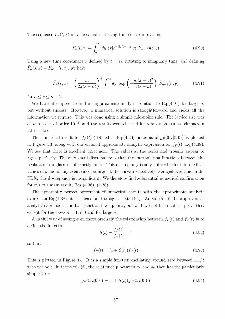
The sequence Fn(t, x) may be calculated using the recursion relation,

Fn(t, x) =

∫ ∞0

dy 〈x|e−iH(t−nε)|y〉 Fn−1(nε, y) (4.90)

Using a new time coordinate s defined by t = sε, rotating to imaginary time, and defining

Fn(s, x) = Fn(−it, x), we have

Fn(s, x) =

(m

2π(s− n)

) 12∫ ∞

0

dy exp

(−m(x− y)2

2(s− n)

)Fn−1(n, y) (4.91)

for n ≤ s ≤ n+ 1.

We have attempted to find an approximate analytic solution to Eq.(4.91) for large n,

but without success. However, a numerical solution is straightforward and yields all the

information we require. This was done using a simple mid-point rule. The lattice size was

chosen to be of order 10−3, and the results were checked for robustness against changes in

lattice size.

The numerical result for fP (t) (defined in Eq.(4.36) in terms of gP (0, t|0, 0)) is plotted

in Figure 4.3, along with our claimed approximate analytic expression for fP (t), Eq.(4.38).

We see that there is excellent agreement. The values at the peaks and troughs appear to

agree perfectly. The only small discrepancy is that the interpolating functions between the

peaks and troughs are not exactly linear. This discrepancy is only noticeable for intermediate

values of n and in any event since, as argued, the curve is effectively averaged over time in the

PDX, this discrepancy is insignificant. We therefore find substantial numerical confirmation

for our our main result, Eqs.(4.36), (4.38).

The apparently perfect agreement of numerical results with the approximate analytic

expression Eq.(4.38) at the peaks and troughs is striking. We wonder if the approximate

analytic expression is in fact exact at these points, but we have not been able to prove this,

except for the cases n = 1, 2, 3 and for large n.

A useful way of seeing even more precisely the relationship between fP (t) and fV (t) is to

define the function

S(t) =fP (t)

fV (t)− 1 (4.92)

so that

fP (t) = (1 + S(t))fV (t) (4.93)

This is plotted in Figure 4.4. It is a simple function oscillating around zero between ±1/3

with period ε. In terms of S(t), the relationship between gP and gV then has the particularly

simple form

gP (0, t|0, 0) = (1 + S(t))gV (0, t|0, 0) (4.94)

67

ææææææææææææææ

ææææææææææææææ

æææææ

æææææææææ

æææææ

æææææææææ

æææææ

æææææææææ

ææææææææææææææ

ææææææææææææææ

ææææææææææææææ

ææææææææææææææ

ææææææææææææææ

ææææææææææææææ

ææææææææææææææ

ææææææææææææææ

ææææææææææææ

ææ

ææææææææææææ

ææ

ææææææææææææ

ææ

ææææææææææææ

ææ

ææææææææææ

ææææ

ææææææææææ

ææææ

ææææææææææ

ææææ

0 5 10 15 20t

0.2

0.4

0.6

0.8

1.0

f HtL

Figure 4.3: A plot of the numerical calculation of fP (t) (the set of dotted lines), and theconjectured analytic expression for fP (t), Eqs.(4.36), (4.38) (the set of straight lines). (Againwe use a time scaling such that ε = 1). There is excellent agreement between analytic andnumerical results at the peaks and troughs of the functions. The numerical result shows somedeparture from exact linear behaviour between the peaks and troughs but this is insignificantas argued in the main text. A plot of fV (t), the smooth curve, is also given for reference.

68

5 10 15 20t

-0.4

-0.2

0.2

0.4

0.6

0.8

1.0SHtL

Figure 4.4: A plot of the function S(t) defined in Eq.(4.92), describing the oscillations ofgP (0, t|0, 0) around gV (0, t|0, 0). The bold line represents the numerical calculation and thedashed line the analytic result (from Eqs.(4.34), (4.38)). After the first few oscillations, itoscillates between ±1/3 (approximately).

69

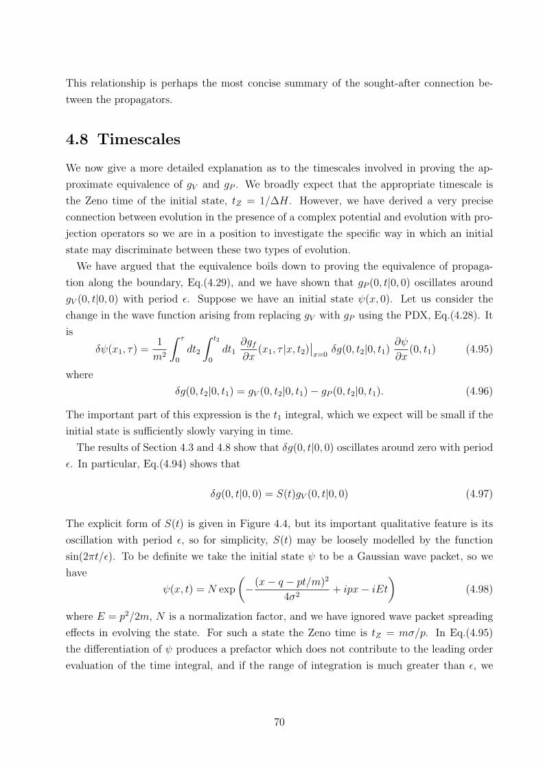
This relationship is perhaps the most concise summary of the sought-after connection be-

tween the propagators.

4.8 Timescales

We now give a more detailed explanation as to the timescales involved in proving the ap-

proximate equivalence of gV and gP . We broadly expect that the appropriate timescale is

the Zeno time of the initial state, tZ = 1/∆H. However, we have derived a very precise

connection between evolution in the presence of a complex potential and evolution with pro-

jection operators so we are in a position to investigate the specific way in which an initial

state may discriminate between these two types of evolution.

We have argued that the equivalence boils down to proving the equivalence of propaga-

tion along the boundary, Eq.(4.29), and we have shown that gP (0, t|0, 0) oscillates around

gV (0, t|0, 0) with period ε. Suppose we have an initial state ψ(x, 0). Let us consider the

change in the wave function arising from replacing gV with gP using the PDX, Eq.(4.28). It

is

δψ(x1, τ) =1

m2

∫ τ

0

dt2

∫ t2

0

dt1∂gf∂x

(x1, τ |x, t2)∣∣x=0

δg(0, t2|0, t1)∂ψ

∂x(0, t1) (4.95)

where

δg(0, t2|0, t1) = gV (0, t2|0, t1)− gP (0, t2|0, t1). (4.96)

The important part of this expression is the t1 integral, which we expect will be small if the

initial state is sufficiently slowly varying in time.

The results of Section 4.3 and 4.8 show that δg(0, t|0, 0) oscillates around zero with period

ε. In particular, Eq.(4.94) shows that

δg(0, t|0, 0) = S(t)gV (0, t|0, 0) (4.97)

The explicit form of S(t) is given in Figure 4.4, but its important qualitative feature is its

oscillation with period ε, so for simplicity, S(t) may be loosely modelled by the function

sin(2πt/ε). To be definite we take the initial state ψ to be a Gaussian wave packet, so we

have

ψ(x, t) = N exp

(−(x− q − pt/m)2

4σ2+ ipx− iEt

)(4.98)

where E = p2/2m, N is a normalization factor, and we have ignored wave packet spreading

effects in evolving the state. For such a state the Zeno time is tZ = mσ/p. In Eq.(4.95)

the differentiation of ψ produces a prefactor which does not contribute to the leading order

evaluation of the time integral, and if the range of integration is much greater than ε, we

70

obtain the order of magnitude result∫dt1 δg(0, t2|0, t1)

∂ψ

∂x(0, t1) ∼ exp

(−t

2Z

ε2(Eε− 1)2

)(4.99)

If Eε � 1, the right-hand side is clearly very small if ε � tZ . If Eε > 2, the right-hand

side if bounded from above by exp(−t2Z/ε2) so again will be small if ε� tZ . Hence the Zeno

time of the initial state is indeed the timescale controlling the validity of the approximation,

as expected. Note also that Eq.(4.99) goes to zero as ε → 0, as it must, since gP and gV

become exactly equal (and equal to gr) in this limit.

The only problematic case is that in which the initial state has energy E ∼ 1/ε. In this

case, the right-hand side of Eq.(4.99) is not necessarily small and the approximation may

fail. This is not surprising since it is the case in which the oscillations in time of the incoming

state are comparable to the temporal spacing of the projections, so that the state can “see”

the difference between the complex potential and projections at a discrete set of times.

Hence, apart from the above exception, Eq.(4.29) holds for ε � tZ . As outlined in the

Introduction to this chapter, reflection from the complex potential is negligible if V0 � E

which is equivalent to ε� 1/E. Therefore there is an interesting regime, namely

1

E� ε� 1

∆H(4.100)

in which the approximate equivalence Eq.(4.29) holds, yet there is negligible reflection. This

regime is important in, for example, study of the arrival time problem using complex poten-

tials [49], and we will make use of it in Chapter 5 of this thesis. (See also Ref.[92] for an

interesting discussion of timescales in the Zeno effect.)

4.9 Summary and Discussion

This chapter was physically motivated by the desire to understand the effect of periodically

acting projections onto the positive x-axis for a free particle, Eq.(4.1). A valuable way to

proceed is to use the conjectured relationship Eq.(4.3) with a complex potential first put

forward by Echanobe et al. This connection, together with known results on scattering,

establishes the timescale under which significant reflection occurs in Eq.(4.1). We noted

that the arguments for the relationship Eq.(4.3) are only heuristic and there is scope for a

more substantial proof.

We proved Eq.(4.3) by considering the associated propagators Eqs.(4.19), (4.20). We

noted that an approximate equivalence between these propagators is expected since both

propagators tend to the restricted propagator gr(x1, τ |x0, 0) in the limits ε → 0, n → ∞

71

and V0 → ∞. The path decomposition expansion reduced the proof of equivalence of these

propagators to the simpler case of propagation between points lying on the origin, Eq.(4.29).

The propagator along the origin for the complex potential gV (0, t|0, 0) is already known,

Eq.(4.34), so the bulk of the proof was to derive the analogous result for the propagator

with projections, gP (0, τ |0, 0). Our main result was to prove that this propagator has the

approximate form Eqs.(4.36), (4.38), which we proved using a variety of analytic and numer-

ical methods. In effect, the main achievement of this chapter has therefore been to obtain a

good approximate analytic expression for the propagator gP that appears in Eq.(4.1).

We found that gP (0, t|0, 0) oscillates with period ε around gV (0, t|0, 0) as long as V0ε ≈ 4/3,

a result most concisely summarized in Eq.(4.94). The approximate equivalence Eq.(4.29) of

these propagators then holds in a time-averaged sense as long as the timescale ε between

projections is much smaller than the Zeno time of the initial state, 1/∆H (but may fail in

the special case when the incoming state is peaked about energy E ∼ 1/ε). These conditions

agree in essence with those of an extended version of the results of Echanobe et al, with an

advantage over their results that a definite relationship between V0 and ε is obtained. We

noted that their restriction Eq.(4.4) relating V0 and ε is in fact stronger than required and

the equality V0ε ≈ 4/3 derived here gives the best approximate equivalence between gP and

gV .

Let us make some comments here on the possible generality of the connection Eq.(4.3).

We first note that it may in fact be written

e−iHεPe−iHε · · ·Pe−iHε ≈ exp(−iHτ − V0P τ

)(4.101)

where P = 1 − P . We have proved Eq.(4.101) for the case in which the projections are

onto the positive x-axis, but it seems reasonably clear that the relationship will hold for

projections onto any region [a, b] of the x-axis (as long as it is not too small) and indeed for

regions of configuration space in a many-dimensional model. Such a potential has been used

recently in the decoherent histories analysis of quantum cosmological models [47]. Moreover,

although the proof of Eq.(4.101) given in this chapter relied heavily on the fact that P

projects onto position, the form Eq.(4.101) and the heuristic argument for it in Section 4.2

do not rely on the particular form of P . We therefore conjecture that Eq.(4.101) may hold

for a wider variety of projection operators, not just projectors onto position. This will be

pursued elsewhere.

Finally we note that the left hand side of Eq.(4.101) is a class operator in the decoherent

histories (DH) approach to quantum theory outlined in Chapter 1. The equivalence expressed

in Eq.(4.101) means we can also use the right hand side as a class operator. The practical

value of this is that it opens the way to dealing with time observables in DH by replacing

72

strings of projectors, which may be hard to work with, with complex potentials which are

much simpler. However on a more fundamental level, it also suggest new ways to construct

class operators which would not have been obvious starting from the exposition in Chapter

1. We will pursue this in the next chapter.

73

5 Arrival Times, Complex Potentials

and Decoherent Histories

Tomorrow, and tomorrow, and tomorrow,

Creeps in this petty pace from day to day

Shakespeare

5.1 Introduction

We saw in the Introduction, Chapter 1, that there are many different approaches to the

arrival time problem in quantum theory, (see Fig.(5.1) for a recap of conventions). The

t1

x

t2

t

Figure 5.1: The quantum arrival time problem. We prepare an initial state localized entirelyin x > 0 and consisting entirely of negative momenta. What is the probability that the particlecrosses the origin during the time interval [t1, t2]?

approach we wish to pursue in the next two chapters is based on the decoherent histories

approach to quantum theory, as outlined in Sections 1.4 and 1.5. We saw in Section 1.5

that the key objects for this analysis are the class operators for crossing and not crossing

74

the origin during a given time interval. The class operator for not crossing was determined

to be,

Cnc(τ) = Pe−iHεP...e−iHεP (5.1)

where P = θ(x), there are N + 1 projections and τ = Nε. In order to avoid the Zeno effect

we need to leave ε finite. However in Section 1.5 we concluded that this object was somewhat

problematic, firstly because we could not determine the required timescale ε, and secondly

because this object is difficult to work with analytically.

However, armed now with the results of Chapter 4 we are able to make progress. The re-

sults of Chapter 4 tell us that evolution with the class operator above, Eq.(5.1), is equivalent

to evolution in the presence of a complex potential,

Cnc(τ) = Pe−iHεP...e−iHεP ≈ e−iHτ−V0P τ , (5.2)

where P = θ(−x), τ = Nε and V0 ∼ 1/ε. Eq.(5.2) holds provided

ε <<1

∆H. (5.3)

This means we can compute the probabilities and the decoherence functional by replacing

class operators of the form Eq.(5.1) with evolution under the complex potential, and this

simplifies the calculations enormously. The equivalence in Eq.(5.2) also tells us that we must

have Eε >> 1, where E is the energy of the incoming state, if we are to avoid reflection.

Of course the results of Chapter 4 as they stand only give us the class operator for not

crossing during a given time interval. We also require the class operator for crossing. We

shall compute this in this chapter, as well as calculating the probabilities and decoherence

functional for questions such as, “Did the particle cross during the time interval [t1, t2]?”

Our end result will be a complete analysis of the arrival time problem in the language of

decoherent histories. Before we do this, however, it is useful to explore some aspects of the

arrival time distribution defined using complex potentials. This will help us to understand

the key features of our final result.

The first aim of this chapter is to look in some detail at the calculation and properties of

the arrival time distribution defined using a complex potential. In particular, we will use

path integral methods, which in some ways are more concise and transparent than previous

derivations. The second aim of this chapter is to carry out a decoherent histories analysis of

the arrival time problem, using the equivalence between strings of projection operators and

complex potentials demonstrated in Chapter 4.

Our main result is that for intervals of size ∆ � 1/V0, these class operators are given

75

approximately by

Ckc = e−iH0τ

∫ tk+1

tk

dt(−1)

2m(p δ(xt) + δ(xt) p)

= e−iH0τ (θ(x(tk))− θ(x(tk+1))) (5.4)

Significantly, the dependence on the complex potential has dropped out entirely. We will

show that there is decoherence for an interesting class of states, and, for such states the

probabilities are then given by

q(tk, tk+1) =

∫ tk+1

tk

dt J(t) (5.5)

This, we will show, coincides with the expected result Eq.(1.8), when Π(t) is integrated over

a range of time much greater than 1/V0. Hence there is complete agreement with standard

results on the arrival time distribution at sufficiently coarse-grained timescales. Furthermore,

our results shed some light on the problem of backflow – we find that the situations when

Eq.(5.5) is negative are those in which there is no decoherence in which case probabilities

cannot be assigned.

In the next Chapter, we compute the crossing class operators in a simpler but more

heuristic way, by exploring a semiclassical approximation to Eq.(5.1) keeping ε finite. The

results are essentially the same.

The rest of this Chapter is arranged as follows: In Section 5.2 we consider the classical

arrival time defined via a complex potential. This well help us understand how the proba-

bilities we obtain depend on the choice of V0, or equivalently ε, in Eq.(5.2). In Section 5.3

we then repeat this analysis for the quantum case, using the PDX to calculate the arrival

time distribution function. We make heavy use in this section of the results of Chapter 2. In

Sections 5.4 and 5.5, we use the results of the previous sections to carry out the decoherent

histories analysis. We summarize and conclude in Section 5.6. This chapter is based on

Ref.[49].

5.2 The Classical Arrival Time Problem via a Complex

Potential

Before looking at the quantum arrival time problem it is enlightening to look at the corre-

sponding classical arrival time problem defined using an absorbing potential. This gives some

understanding of the expected form of the result in the quantum case. In particular since

the complex potential is a simple measurement model we expect the probabilities obtained

76

in this way to be of the form Eq.(1.27), which include an “apparatus response function.”

We will see in this section that exactly the same thing happens in the classical case, and in

fact the response functions are the same in the quantum and classical cases. This means the

complex potential is acting like a classical measuring device, and all dependence on it can

be removed by coarse-graining, in the manner of Eq.(1.28).

We consider a classical phase space distribution wt(p, q), with initial value w0(p, q) con-

centrated entirely in q > 0 with only negative momenta. This distribution evolves in the

presence of a complex potential V (q) = −iV0θ(−q). The equation of motion is,

∂w

∂t= − p

m

∂w

∂q− 2V (q)w. (5.6)

This form may be deduced, for example, by computing the evolution equation of the Wigner

function with this complex potential and dropping the higher order terms (involving powers

of h). Eq.(5.6) is readily solved and has solution

wτ (p, q) = exp

(−2

∫ τ

0

ds V (q − ps/m)

)w0(p, q − pτ/m) (5.7)

The survival probability, that is the probability of not having been absorbed by the com-

plex potential by a time τ , is

N(τ) =

∫ ∞−∞

dp

∫ ∞−∞

dq wτ (p, q). (5.8)

The arrival time distribution is therefore

Π(τ) = −dNdτ

= 2V0

∫ ∞−∞

dp

∫ 0

−∞dq wτ (p, q) (5.9)

where we have made use of Eq.(5.6). This expression is conveniently rewritten by noting

that, again using Eq.(5.6), Π(τ) obeys the equation

dΠ

dτ+ 2V0Π = −2V0

∫ ∞−∞

dpp

mwτ (p, 0) (5.10)

This may be solved to yield

Π(τ) = −2V0

∫ τ

0

dt e−2V0(τ−t)∫ ∞−∞

dpp

mwt(p, 0) (5.11)

77

From Eq.(5.7), we see that

wt(p, 0) = exp

(−2V0

∫ t

0

ds θ(ps/m)

)w0(p,−pt/m) (5.12)

but since the momenta are all negative the exponential factor makes no contribution. We

thus obtain

Π(τ) = 2V0

∫ τ

0

dt e−2V0(τ−t) J(t) (5.13)

where

J(t) = −∫ ∞−∞

dpp

mw0(p,−pt/m) (5.14)

The current J(t) is the usual classical arrival time distribution that we would have expected

in the absence of the absorbing potential.

Eq.(5.13) has the same form as the expressions for the quantum arrival time we expect to

obtain from a measurement model, Eq.(1.27). The response function is given by the quantity,

R(τ, s) = 2V0 exp(−2V0(τ − s)). (5.15)

In Chapter 1 we noted that R(τ, s) is related to a sort of coarse graining in time, we now

demonstrate this for this specific case. Eq.(5.13) gives the probability Π(τ)dτ for arriving

during the infinitesimal time interval [τ, τ + dτ ]. Supposer we consider the probability for

arriving during a finite time interval, [τ1, τ2]. This is given by

p(τ2, τ1) =

∫ τ2

τ1

dτ Π(τ)

=

∫ τ2

τ1

dτ

∫ τ

0

dt 2V0 e−2V0(τ−t) J(t) (5.16)

Rearranging the order of integration and integrating over τ yields,

p(τ2, τ1) =

∫ τ1

0

dt

∫ τ2

τ1

dτ 2V0 e−2V0(τ−t) J(t)

+

∫ τ2

τ1

dt

∫ τ2

t

dτ 2V0 e−2V0(τ−t) J(t) (5.17)

=

∫ τ1

0

dt(e−2V0(τ1−t) − e−2V0(τ2−t)

)J(t)

+

∫ τ2

τ1

dt(1− e−2V0(τ2−t)

)J(t) (5.18)

1/V0 plays a role as a fundamental short timescale in the problem, so now suppose we assume

that τ1, τ2 and (τ2 − τ1) are all much greater than 1/V0. It follows that all the exponential

78

terms may be dropped in Eq.(5.18) and we obtain the very simple result,

p(τ2, τ1) ≈∫ τ2

τ1

dt J(t) (5.19)

That is, all dependence on the resolution function R(τ, s) and the complex potential pa-

rameter V0 completely drops out when we look at probabilities defined on timescales much

greater than 1/V0. This result is very relevant to the decoherent histories analysis considered

later where it is natural to look at the arrival time during a finite time interval much greater

than ε.

5.3 Calculation of the Arrival Time Distribution via a

Complex Potential

We now repeat the analysis of the previous section for the quantum case. The analogue of

Eq.(5.6) is the inclusion of the complex potential,

V (x) = −iV0θ(−x) (5.20)

in the Schrodinger equation. With such a potential, the state at time τ is

|ψ(τ)〉 = exp (−iH0τ − V0θ(−x)τ) |ψ〉 (5.21)

where H0 is the free Hamiltonian. In a similar way to the classical case the idea is that

the part of the wave packet that reaches the origin during the time interval [0, τ ] should be

absorbed, so that

N(τ) = 〈ψ(τ)|ψ(τ)〉 (5.22)

is the probability of not crossing x = 0 during the time interval [0, τ ]. The probability of

crossing between τ and τ + dτ is then

Π(τ) = −dNdτ

(5.23)

Complex potentials such as Eq.(5.20) were originally considered by Allcock in his seminal

work on arrival time [6] and have subsequently appeared in detector models [44, 18]. (See

also Ref.[76, 62] for further work with complex potentials). From the results of Chapter 4 we

see that evolution according to Eq.(5.21) is essentially the same as evolution under pulsed

measurements.

For large V0, the wave function defined by the evolution Eq.(5.21) undergoes significant

79

reflection, with total reflection in the “Zeno limit”, V0 →∞ [74]. Here, we are interested in

the opposite case of small V0, where there is small reflection and Eq.(5.23) can give reasonable

expressions for the arrival time distribution. A number of different authors [6, 18, 62] indicate

that the resulting distribution is of the form

Π(τ) =

∫ ∞−∞

dt R(V0, τ − t)J(t) (5.24)

where J(t) is the current,

J(t) = 〈ψ0| (−1)

2m{pδ(x) + δ(x)p} |ψ0〉

=i

2m

(ψ∗(0, τ)

∂ψ(0, τ)

∂x− ∂ψ∗(0, τ)

∂xψ(0, τ)

)(5.25)

and,

R(V0, t) = 2V0θ(t) exp (−2V0t) (5.26)

It is therefore closely related to the current J(t) but also includes the influence of the complex

potential via the “apparatus resolution function” R(V0, t). Our aim in this section is to prove

this claim.

With the complex potential Eq.(5.20), the arrival time distribution Eq.(5.23) is given by

Π(τ) = 2V0〈ψτ |θ(−x)|ψτ 〉 (5.27)

where

|ψτ 〉 = exp (−iHτ) |ψ〉= exp (−iH0τ − V0θ(−x)τ) |ψ〉 (5.28)

(so we use H = H0 − iV0θ(−x) to denote the total non-Hermitian Hamiltonian). We are

interested in calculating this expression for the case in which V0 is much smaller than the

energy scale of the initial state. (The very different limit, of V0 → ∞, the Zeno limit, has

been explored elsewhere [45]).

One way to evaluate Eq.(5.27) is to use the transmitted wave functions, Eq.(2.17). How-

ever, we give here instead a different and more direct derivation using the PDX. We use the

first crossing PDX, written in operator form, Eq.(2.13),

〈x| exp(−iHτ)|ψ〉 = − 1

m

∫ τ

0

dt 〈x| exp(−iH(τ − t)) δ(x)p exp (−iH0t) |ψ〉 (5.29)

80

Now note that the operator δ(x) = |0〉〈0| has the simple property that for any operator A

δ(x)Aδ(x) = δ(x)〈0|A|0〉 (5.30)

(where, recall, |0〉 denotes the position eigenstate |x〉 at x = 0). Inserting Eq.(5.29) in

Eq.(5.27), together with the property Eq.(5.30) and the change of variables s = τ − t,

s′ = τ − t′, yields

Π(τ) =2V0

m2

∫ τ

0

ds′∫ τ

0

ds

∫ 0

−∞dx

× 〈0| exp(iH†s′

) |x〉〈x| exp (−iHs) |0〉× 〈ψ| exp (iH0(τ − s′)) p δ(x) p exp (−iH0(τ − s)) |ψ〉 (5.31)

We are aiming to show that this coincides with Eq.(5.24) with the current Eq.(5.25), and the

main challenge is to show how the pδ(x)p combination turns into the combination pδ(x) +

δ(x)p in the current Eq.(5.25).

Consider first the x integral. Since we are assuming small V0, we may use the semiclassical

approximation Eq.(2.25), which reads

〈x| exp (−iHs) |0〉 ≈( m

2πis

)1/2

exp

(imx2

2s− V0s

)(5.32)

The x integral may now be carried out, with the result,

Π(τ) =V0

m2

∫ τ

0

ds′∫ τ

0

ds( m

2πi

)1/2 e−V0(s+s′)

(s− s′) 12

× 〈ψτ | exp (−iH0s′) p δ(x) p exp (iH0s) |ψτ 〉 (5.33)

where |ψτ 〉 denotes the free evolution of the initial state.

We now carry out one of the time integrals. Note that,∫ τ

0

ds′∫ τ

0

ds =

∫ τ

0

ds′∫ τ

s′ds+

∫ τ

0

ds

∫ τ

s

ds′ (5.34)

In the first integral, we set u = s′, v = s − s′, and in the second integral we set u = s,

81

v = s′ − s. We thus obtain

Π(τ) =V0

m2

(m2π

)1/2∫ τ

0

du e−2V0u

∫ τ−u

0

dve−V0v

v12

×[

1

i12

〈ψτ | exp (−iH0u) p δ(x) p exp (iH0(u+ v)) |ψτ 〉

+1

(−i) 12

〈ψτ | exp (−iH0(u+ v)) p δ(x) p exp (iH0u) |ψτ 〉]

(5.35)

The factors of 1/(±i) 12 in front of each term come from a careful consideration of the square

root in the free propagator prefactor (and must have this form because Π(τ) is real).

We will assume that V0τ � 1, which means that the integrals are concentrated around

u = v = 0. This means that we may take the upper limit of the v integral to be ∞, and it

may be carried out, to yield,

Π(τ) = 2V0

∫ τ

0

du e−2V0u

× 1

2m〈ψτ−u| p δ(x) Σ(p) + Σ†(p) δ(x) p |ψτ−u〉 (5.36)

where the operator Σ(p) is given by

Σ(p) =p

[2m(H0 + iV0)]12

(5.37)

For V0 much less than the energy scale,

Σ(p) ≈ p

|p| (5.38)

so Σ(p) is simply the sign function of the momentum, which is −1 in this case, since the

initial state consists entirely of negative momenta. Finally, writing u = τ − t, we obtain

Π(τ) = 2V0

∫ τ

0

dt e−2V0(τ−t) (−1)

2m〈ψt| (p δ(x) + δ(x) p) |ψt〉

= 2V0

∫ τ

0

dt e−2V0(τ−t) J(t) (5.39)

We therefore have precise confirmation of the classical result Eq.(5.13), and also agreement

with the expected quantum result, Eq.(5.24).

Some comments are in order concerning the positivity of the result for Π(τ). The ex-

pression (5.36) is positive because it was derived from the manifestly positive expression

82

Eq.(5.31). (Two approximations were used: the semiclassical approximation Eq.(5.32), and

the condition V0τ � 1, neither of which affect the positivity of the result.)

However, to obtain the final result Eq.(5.39) we took the limit V0 → 0 in the current part

only of Eq.(5.36), leaving behind the V0-dependent term in the exponential part, and the

resulting expression is not guaranteed to be positive. In Eq.(5.39), J(t) is not always positive

due to the backflow effect [78, 12] and integration over time does not necessarily remedy the

situation. (See the Appendix for a more thorough discussion of this point). The lack of

positivity for a Π(τ) obtained in this way is not surprising since taking the limit V0 → 0 in

one part of the expression Eq.(5.36) only but not the other will not necessarily preserve its

property of positivity. The violation of positivity is generally small, however, so Eq.(5.39)

may still be a good approximation to the manifestly positive expression Eq.(5.36).

It should also be added that it would be misleading to explore the first order corrections

in V0 in going from Eq.(5.36) to Eq.(5.39), since comparable correction terms have already

been dropped in using the semiclassical approximation Eq.(5.32).

5.4 Decoherent Histories Analysis for a Single Large

Time Interval

We turn now to the decoherent histories analysis of the arrival time problem. The important

question we wish to answer is; What is the probability of arriving during some general time

interval [t1, t2]? We answer this question in detail in the next section, here we address a

simpler question; What are the probabilities for crossing or not crossing during the large

time interval [0, τ ]? The reason for tackling this question first is that it gives us useful

insight into the more general case and also suggests an interesting way of thinking about the

situations in which we might have decoherence.

The class operators for not crossing and crossing during this time interval are

Cnc = exp (−iH0τ − V0θ(−x)τ) (5.40)

Cc = exp (−iH0τ)− exp (−iH0τ − V0θ(−x)τ) (5.41)

and they satisfy

Cnc + Cc = e−iH0τ (5.42)

We are interested in the probabilities for not crossing and crossing,

pnc(τ) = Tr(CncρC

†nc

)(5.43)

pc(τ) = Tr(CcρC

†c

)(5.44)

83

and the off-diagonal term of the decoherence functional,

Dc,nc = Tr(CncρC

†c

)= Tr

(Cncρe

iH0τ)− pnc (5.45)

These quantities obey the relation

pnc + pc +Dc,nc +D∗c,nc = 1 (5.46)

We look for situations where there is decoherence,

Dc,nc = 0 (5.47)

(which is usually only approximate), in which case the probabilities then sum to 1,

pc(τ) + pnc(τ) = 1 (5.48)

It is useful to relate some of these expressions to the standard expressions for arrival time

Π(t) defined in Eqs.(5.22), (5.23). To do this, note that pnc is in fact the same as the survival

probability, N(τ) defined in Eq.(5.22), and that pnc obeys the trivial identity

pnc(τ) = 1 +

∫ τ

0

dtdpncdt

(5.49)

since pnc(0) = 1. It follows that

pnc(τ) = 1−∫ τ

0

dt Π(t) (5.50)

When there is decoherence, Eq.(5.48) holds and we may deduce that

pc(τ) =

∫ τ

0

dt Π(t) (5.51)

Hence the decoherent histories analysis is compatible with the standard result, but only

when there is decoherence.

We turn now to the calculation of the decoherence functional. Following the general

pattern described in Eqs.(1.32), (1.33), consider the quantity,

qnc(τ) = Tr(Cncρe

iH0τ)

(5.52)

84

From Eq.(5.45), we see that the decoherence functional may be written,

Dc,nc = qnc(τ)− pnc(τ) (5.53)

This means that qnc = pnc when there is decoherence. Or to put it the other way round,

decoherence of histories may be checked by comparing qnc with pnc and this is what we now

do. Recall that pnc is given by Eqs.(5.49), (5.50) (which hold in the absence of decoherence).

We may write qnc in a similar form:

qnc(τ) = 1 +

∫ τ

0

dtdqncdt

(5.54)

The integrand is similar to Π(t) defined in Eq.(5.27), so we define

Π(t) ≡ −dqncdt

(5.55)

We now have that

qnc(τ) = 1−∫ τ

0

dt Π(t) (5.56)

It then follows that the decoherence functional is

Dc,nc =

∫ τ

0

dt(

Π(t)− Π(t))

(5.57)

To compute the decoherence functional we need to calculate Π(t), which is given by

Π(t) = V0〈ψ| exp (iH0t) θ(−x) exp (−iH0t− V0θ(−x)t) |ψ〉 (5.58)

This is almost the same as Π(t) except that the exponential on the left involves only H0

and not the complex potential (and also an overall factor of 2). We therefore follow the

calculation of Π(t) in Section 5.3 with small modifications. With a little care, one may see

that the final result is the same as that for Π(t), Eq.(5.39), except that 2V0 is replaced with

V0, that is,

Π(t) = V0

∫ t

0

ds e−V0(τ−s) J(s) (5.59)

This result holds for timescales greater than 1/V0 and under the semiclassical approxima-

tion (which required E � V0 so is equivalent to the requirement of negligible reflection

encountered above). Finally, a calculation similar to that of Eqs.(5.16)-(5.19) implies that∫ τ

0

dt Π(t) ≈∫ τ

0

dt J(t) (5.60)

85

as long as V0τ � 1. Since this result is independent of V0, Π(t) will satisfy the same relation.

We thus deduce that

Dc,nc ≈ 0 (5.61)

hence there is decoherence, under the above conditions.

This analysis gives us an interesting way of thinking about decoherence. Decoherence is

achieved if Eq.(5.59) is equal to Eq.(5.39). This will be the case if the current varies on a

timescale that is long compared with 1/V0 >> 1/E, where E is the energy of the wavepacket.

The timescale on which the current varies is given, for a gaussian wavepacket, as 1/∆H. In

Chapter 4 we noted that whereas the timescale given by 1/E is genuinely quantum, 1/∆H is

in fact a classical timescale. This means we will have decoherence if there is a large separation

between the quantum and classical timescales associated with the incoming wavepacket, a

satisfying result.

5.5 Decoherent Histories Analysis for an Arbitrary Set

of Time Intervals

We now turn to the more complicated question of much more refined histories, that may

cross the origin at any one of a large number of times, during the time interval [0, τ ]. This

corresponds more directly to the standard crossing probability, Π(t)dt, the probability that

the particle crosses during an infinitesimal time interval [t, t+ dt].

5.5.1 Class Operators

We have defined class operators Eqs.(5.40), (5.41) describing crossing or not crossing during

a time interval [0, τ ]. We now split this time interval into n equal parts of size ε, so τ = nε

and we seek class operators describing crossing or not crossing during any one of the n

intervals. We first note that

e−iH0ε = Cnc(ε) + Cc(ε) (5.62)

where Cnc(ε) and Cc(ε) are defined as in Eqs.(5.40), (5.41) except that here they are for a

time interval [0, ε]. We now use this to decompose e−iH0τ into the desired class operators.

We have

e−iH0τ =(e−iH0ε

)n=

(e−iH0ε

)n−1(Cnc(ε) + Cc(ε))

=(e−iH0ε

)n−1Cnc(ε) + e−iH0(τ−ε)Cc(ε) (5.63)

86

Repeating the same steps on the first term, this yields,

e−iH0τ =(e−iH0ε

)n−2Cnc(2ε) + e−iH0(τ−2ε)Cc(ε)Cnc(ε) + e−iH0(τ−ε)Cc(ε) (5.64)

Repeating more times eventually yields,

e−iH0τ = Cnc(τ) +n−1∑k=0

e−iH0(τ−(k+1)ε)Cc(ε)Cnc(kε) (5.65)

From this expression, we see that the class operator for crossing x = 0 for the first time

during the time interval [kε, (k + 1)ε] is given by the summand of the second term,

Cc((k + 1)ε, kε) = e−iH0(τ−(k+1)ε)Cc(ε)Cnc(kε) (5.66)

We will not in fact work with the class operator Eq.(5.66), since a more useful similar

but alternative expression can also be found. Taking the continuum limit of Eq.(5.65) (and

inserting the explicit expression for Cnc), we obtain,

e−iH0τ = e−iH0τ−V τ +

∫ τ

0

dt e−iH0(τ−t)V e−iH0t−V t (5.67)

(where, recall, V = V0θ(−x)). This indicates that the class operator for first crossing during

the infinitesimal time interval [t, t+ dt], is

Cc(t) = e−iH0(τ−t)V e−iH0t−V t (5.68)

We do not, however, expect histories characterized by such precise crossing time to be

decoherent, so it is natural to consider coarser-grained class operators,

Ckc =

∫ tk+1

tk

dt Cc(t) (5.69)

which represents crossing during one of theN time intervals [tk, tk+1] of size ∆, where tk = k∆

with k = 0, 1 · · ·N − 1 and τ = N∆. The complete set of class operators Cα for crossing

and not crossing is the set of N + 1 operators

Cα = {Cnc, Ckc } (5.70)

87

and Eq.(5.67) implies that they satisfy

e−iH0τ = Cnc +N−1∑k=0

Ckc (5.71)

To check for decoherence of histories we need to calculate two types of decoherence functional

Dkk′ = Tr(Ckc ρ(Ck′

c )†)

(5.72)

Dk,nc = Tr(Ckc ρ(Cnc)

†) (5.73)

and this will be carried out below.

5.5.2 An Important Simplification of the Class Operator

There turns out to be a very useful simplification in the class operator Eq.(5.68). Consider

the amplitude

〈x|eiH0τCc(t)|ψ〉 = V0〈x|e−iH0tθ(−x)e−iH0t−V t|ψ〉 (5.74)

for any x. The right-hand side is very similar to Eq.(5.27), except that there is no complex

potential in one of the exponential terms and also the “final” state is |x〉 not |ψ〉. (And there

is also an overall factor of 2 different). Despite these differences, we may once again make

use of the details of the calculation of Section 5.3, and we deduce from the analogous result

Eq.(5.39), that

〈x|eiH0τCc(t)|ψ〉 = V0

∫ t

0

ds e−V0(t−s) (−1)

2m〈x| (p δ(xs) + δ(xs) p) |ψ〉 (5.75)

Like the derivation of Eq.(5.39), this is valid under the conditions that all energy scales

are much greater than V0 and all time scales much greater than 1/V0. Now we integrate

this over time to obtain the coarse-grained crossing time operator, Eq.(5.69), and again use

approximations of the form Eqs.(5.16)-(5.19) (again using the assumption of timescales much

greater than 1/V0), to yield, the remarkably simple and appealing form,

eiH0τCkc =

∫ tk+1

tk

dt(−1)

2m(p δ(xt) + δ(xt) p) (5.76)

This may also be written even more simply

eiH0τCkc = θ(x(tk))− θ(x(tk+1)) (5.77)

88

5.5.3 Probabilities for Crossing

The above expressions for the crossing time class operator are the most important results of

this Chapter and provide an immediate connection to the standard expression for the arrival

time distribution. Supposing for the moment that there is decoherence of histories, we may

assign probabilities to the histories. The probability for crossing during the time interval

[tk, tk+1] is

p(tk, tk+1) = Tr(Ckc ρ(Ck

c )†)

(5.78)

However, as noted in Eqs.(1.32), (1.33) when there is decoherence of histories, this expression

for the probabilities for histories is equal to the simpler expression,

q(tk, tk+1) = Tr(Ckc ρe

iH0τ)

=

∫ tk+1

tk

dt(−1)

2m〈ψ| (p δ(xt) + δ(xt) p) |ψ〉

=

∫ tk+1

tk

dt J(t), (5.79)

which is precisely the standard result! The expression for the probability q(tk, tk+1) is not

positive in general (although is real in this case, as it happens), but when there is decoherence,

it is equal to p(tk, tk+1), which is positive. Hence the decoherent histories result coincides

with the standard result under the somewhat special conditions of decoherence of histories.

5.5.4 Decoherence of Histories and the Backflow Problem

There is an interesting connection between decoherence of histories and backflow. To see this,

consider the following simple case. We consider histories which either cross or do not cross

the origin during the time interval [t1, t2]. So the crossing and not crossing class operators

are C and 1− C, where

C = θ(x1)− θ(x2) (5.80)

where we have adopted the notation xk = x(tk) (and for convenience we have dropped the

exponential factor which is just a matter of definition and drops out of all expression of

interest). The decoherence functional is

D = 〈C(1− C)〉= 〈C〉 − 〈C2〉 (5.81)

89

This may also be written

D = −〈(θ(−x1)θ(x2) + θ(x2)θ(−x1))〉 (5.82)

a form we will use below to check decoherence. When there is decoherence, D = 0 and the

probability for crossing is

p(t1, t2) = 〈C2〉 = 〈C〉 (5.83)

As noted above, 〈C〉 is the standard result, Eq.(5.79), for the probability of crossing.

There is an interesting connection here between backflow and decoherence. If there is

decoherence, D is zero so 〈C〉 must cancel 〈C2〉 in Eq.(5.81), which means that 〈C〉 ≥ 0, so

there is no backflow. Or we may make a logically equivalent statement: if there is backflow,

〈C〉 < 0, then there cannot be decoherence, since |D| is then greater than the probability

〈C2〉. Hence, states with backflow do not permit decoherence of histories. (Note that absence

of backflow, 〈C〉 ≥ 0, is not itself enough to guarantee decoherence – the stronger condition

D = 0 must be satisfied).

This is an important result. The quantity 〈C〉 is regarded as the “standard” result for

the arrival time probability and its possible negativity is disturbing. Here, the decoherent

histories approach sheds new light on this issue. In the decoherence histories apporach, the

true probability for crossing is the manifestly positive quantity 〈C2〉 and this is equal to

〈C〉 only when there is decoherence. In particular, when there is significant backflow, there

cannot be decoherence, so probabilities cannot be assigned and 〈C2〉 is not equal to 〈C〉.

5.5.5 The Decoherence Conditions

The crossing probabilities described above are only valid when all components of the deco-

herence functional, Eqs.(5.72), (5.73), are zero. We therefore address the issue of finding

those states for which these conditions hold.

The most important decoherence condition is that Dkk′ defined in Eq.(5.72) vanishes, so

we focus on that. We write the class operator Eq.(5.77) for crossing during the time interval

[tk, tk+1] as

Ckc = e−iH0τ (θ(xk)− θ(xk+1)) (5.84)

For an initial state |ψ〉, the quantity Ckc |ψ〉 is a quantum state representing the property

of crossing of the origin in the time interval [tk, tk+1]. The decoherence condition Dkk′ = 0

is simply the condition that the “crossing states” Ckc |ψ〉 for different time intervals have

negligible interference. The states Ckc |ψ〉 consist of an initial state which has been localized

to a range of time at x = 0. This is closely related to the interesting question of diffraction

in time [75] and this connection will be explored in more detail elsewhere [53].

90

The decoherence functional is given by

Dkj = 〈(θ(xk)− θ(xk+1)) (θ(xj)− θ(xj+1))〉= 〈(θ(xk)− θ(xk+1)) (θ(−xj+1)− θ(−xj))〉 (5.85)

where without loss of generality we take tj+1 < tk. It is a sum of terms each of the form,

dkj = 〈θ(−xk)θ(xj)〉 (5.86)

where tk < tj. Note that

|dkj|2 ≤ d2m = 〈θ(−xk)θ(xj)θ(−xk)〉 (5.87)

The key thing is that d2m has the form of a probability – it is the probability to find the

particle in x < 0 at tk and then in x > 0 at tj. Semiclassical expectations suggest that this

is small in general for the states considered here, which are left-moving wave packets, and

indeed the classical limit of this probability is zero. So this is a useful object to calculate

in terms of checking decoherence. (Although it may not be small for states with backflow).

Note that it also implies that the other parts of the decoherence functional, Eq.(5.85) will

also be small. In detailed calculations, the upper bound Eq.(5.87) must be compared with

the probabilities, as in Eq.(1.40).

5.5.6 Checking the Decoherence Condition for Wavepackets

Decoherence starts to become lost as the the size ∆ of the time intervals [tk, tk+1] is reduced to

close to 1/E. This is because the “localisation in time” produces a corresponding spreading

in energy, and thus momentum, and for sufficiently small time intervals this is enough to

give rise to positive momenta with significant probability. We will see in a specific example

how this works.

For simplicity we work with the simple wavepacket initial states, more general initial states

require an environment to produce decoherence and will be considered in Chapter 7. We

take the initial state to be,

ψ(x) =1

(2πσ2)1/4exp

(−(x− q0)2

4σ2+ ip0x

)(5.88)

where q0 > 0, p0 < 0 and |p0|σ >> 1. We note that the decoherence functional Eq.(5.82)

satisfies

|D|2 ≤ 2d2m (5.89)

91

with d2m given by Eq.(5.87) with k = 1, j = 2. We need some probabilities to compare this

with. We have that

|D|2 ≤ 〈C2〉〈(1− C)2〉 (5.90)

The interesting case is that in which the crossing probability 〈C2〉 is somewhat less than 1,

less than about 1/2, say, in which case the non-crossing probability 〈(1 − C)2〉 will be of

order 1. It is therefore sufficient to compare d2m with 〈C2〉. Now note that

〈C2〉 = 〈(θ(x1)− θ(x2))2〉= 〈θ(x1)θ(−x2)θ(x1)〉+ 〈θ(x1)θ(−x2)θ(−x1)〉+ 〈θ(x2)θ(−x1)〉. (5.91)

This means that 〈C2〉 is in fact equal to the probability,

p12 = 〈θ(x1)θ(−x2)θ(x1)〉, (5.92)

up to terms which vanish when D = 0. This is useful since it is now identical in form to the

expression for d2m and our goal is to show that

d2m � p12. (5.93)

It is useful to work in the Wigner representation [10], defined, for a state ρ(x, y) by

W (p, q) =1

2π

∫dξ e−ipξ ρ(q +

1

2ξ, q − 1

2ξ). (5.94)

The probabilities p12 and d2m are then given by

p12 = 2π

∫dpdq WP (p, q) W0(p, q, t1), (5.95)

d2m = 2π

∫dpdq WD(p, q) W0(p, q, t1). (5.96)

Here, W0(p, q, t1) is the Wigner function of the initial state, evolved in time to t1,

W0(p, q, t1) =1

πexp

(−(q − q0 − p0t1/m)2

2σ2− 2σ2(p− p0)2

). (5.97)

The objects WP and WD are the Wigner transforms of the θ-function combinations appearing

92

in Eqs.(5.87), (5.92) and are given by

WP (p, q) =1

2π2θ(q)

∫ ∞u(p,q)

dysin y

y, (5.98)

WD(p, q) =1

2π2θ(−q)

∫ ∞u(p,q)

dysin y

y, (5.99)

where

u(p, q) = 2q

(p+

mq

(t2 − t1)

). (5.100)

We see that the only difference between the expressions for p12 and d2m is in the sign in the

θ-functions.

The integral

f(u) =

∫ ∞u

dysin y

y(5.101)

may be expressed in terms of the Sine integral function Si(x),

f(u) =π

2− Si(u) (5.102)

but its properties are not hard to see directly. For large negative u, f(u) ≈ π, at u = 0,

f(0) = π/2, and for large positive u, f(u) goes to zero, oscillating around 1/u. (See Figure

5.2.)

-20 -10 10 20u

0.5

1.0

1.5

2.0

2.5

3.0

3.5f HuL

Figure 5.2: The function f(u). It oscillates around zero for u � 0 and oscillates around πfor u� 0. As a function of q, f(u(p0, q)) differs from 0 or π only in a region of size 1/|p0|around q = 0.

93

We now compare the size of p12 and d2m.We assume that the wave packet is spatially broad,

so σ is large and the Wigner function Eq.(5.97) is therefore concentrated strongly about

p = p0 < 0. We therefore integrate out p and set p = p0 throughout. The most important

case to check is that in which the wave packet is reasonably evenly divided between x > 0

and x < 0 at time t1 so that both p12 and d2m have a chance of being reasonably large. This

means that q0 + p0t1/m should be close to zero (to within a few widths σ), so for simplicity

we take it to be exactly zero.

With these simplifications, we have

d2m =

1

(2π3σ2)1/2

∫ 0

−∞dq exp

(− q2

2σ2

)f(u(p0, q)). (5.103)

Here, since q ≤ 0 and p0 < 0, we have u(p0, q) ≥ 0. We can evaluate this expression by

examining the comparative effects of f(u) and the exponential term. From the plot of f(u)

(see Figure 5.2), we see that it drops to zero at u = u0 (which is of order 1) and oscillates

rapidly around zero for u > u0, so we expect the integral to be dominated by values of q for

which 0 ≤ u ≤ u0. The value u = u0 corresponds to q = q0 where

q0 = −|p0|∆2m

([1 +

u0

E0∆

]1/2

− 1

), (5.104)

where E0 = p20/2m. In the complex potential calculations, we have assumed that E0 � V0

and we also assumed that all timescales are much greater than 1/V0, and these together

imply that E0∆� 1. We may therefore expand the square root to leading order and obtain

q0 ≈ − u0

2|p0| . (5.105)

We have assumed that the wave packet is sufficiently broad that σp0 � 1, and this means

that

|q0| � σ. (5.106)

This in turn means that f(u) is significantly different from zero only in the range |q| � σ,

and most importantly, in this range, the exponential term in Eq.(5.103) is approximately

constant. We may therefore evaluate Eq.(5.103) by ignoring the exponential term, integrating

from 0 to q0 and approximating f(u) as

f(u) ≈ π

2− u+O(u3). (5.107)

94

We thus obtain the simple result,

d2m ≈

1

(2π3)1/2

1

|p0|σ � 1. (5.108)

In the expression for p12, there is a key difference in that q > 0 which means that u(p0, q)

can be positive or negative. Introducing

qz =|p0|m

∆ = σ∆

tz(5.109)

(where tz is the Zeno time) we see that u < 0 for q < qz and u > 0 for q > qz. We therefore

have

p12 =1

(2π3σ2)1/2

∫ qz

0

dq exp

(− q2

2σ2

)f(u(p0, q))

+1

(2π3σ2)1/2

∫ ∞qz

dq exp

(− q2

2σ2

)f(u(p0, q)). (5.110)

Here, f(u(p0, q)) ≈ π in the first term, differing from this value only in a region of size 1/p0

close to q = 0. In the second term f(u) will tend to be small except for a small region of

size 1/p0 around the origin.

If qz � σ, (that is, ∆� tz), the second term in p12 is exponentially suppressed and in the

first term the integration range is effectively 0 to ∞, so we obtain

p12 ≈ 1

2. (5.111)

This is the expected result, since under the above assumptions on the wave packet, half of

it will cross x = 0 if the time interval is sufficiently large. Clearly p12 � d2m in this case so

there is decoherence.

If qz � σ, the first term in p12 is of order qz/σ and the second of order 1/(|p0|σ), the same

order of magnitude as d2m. Hence in this case we have decoherence if

∆

tz� 1

|p0|σ , (5.112)

which is equivalent to,

E∆� 1. (5.113)

Crucially this is equivalent to the condition that there be negligible reflection from the

complex potential.

In brief, we therefore get decoherence of histories for a single wave packet under a wide

95

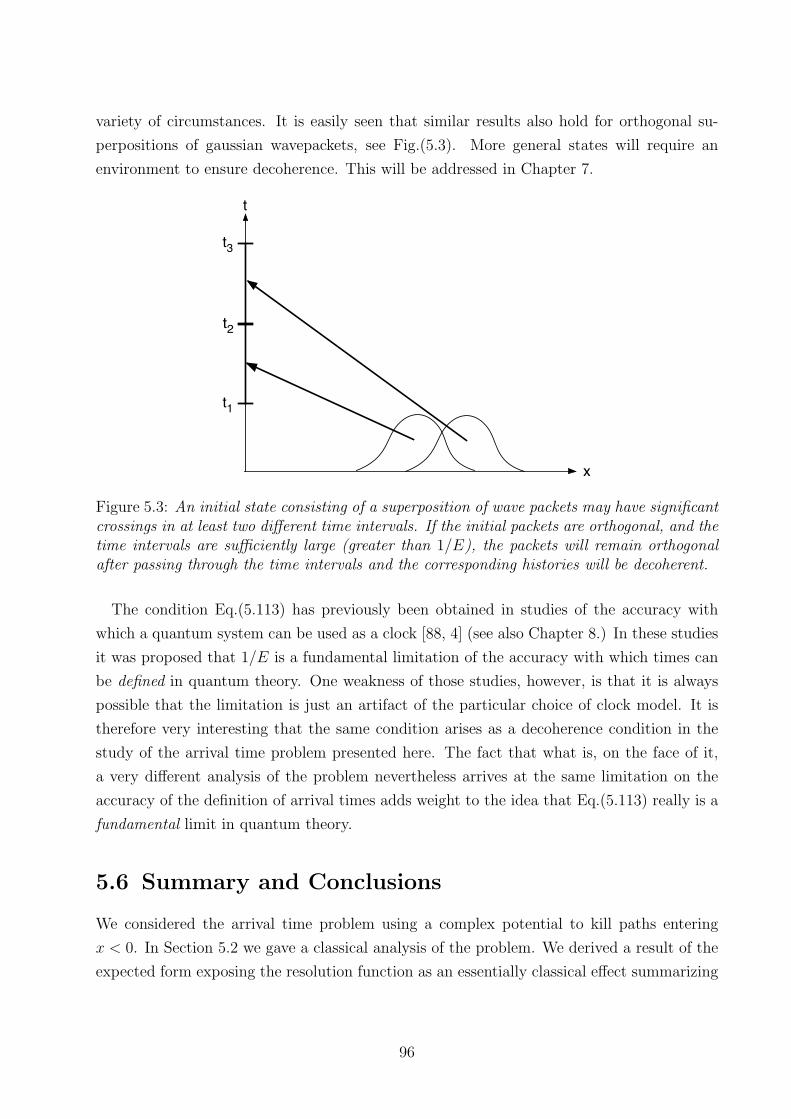
variety of circumstances. It is easily seen that similar results also hold for orthogonal su-

perpositions of gaussian wavepackets, see Fig.(5.3). More general states will require an

environment to ensure decoherence. This will be addressed in Chapter 7.

x

t1

t2

t

t3

Figure 5.3: An initial state consisting of a superposition of wave packets may have significantcrossings in at least two different time intervals. If the initial packets are orthogonal, and thetime intervals are sufficiently large (greater than 1/E), the packets will remain orthogonalafter passing through the time intervals and the corresponding histories will be decoherent.

The condition Eq.(5.113) has previously been obtained in studies of the accuracy with

which a quantum system can be used as a clock [88, 4] (see also Chapter 8.) In these studies

it was proposed that 1/E is a fundamental limitation of the accuracy with which times can

be defined in quantum theory. One weakness of those studies, however, is that it is always

possible that the limitation is just an artifact of the particular choice of clock model. It is

therefore very interesting that the same condition arises as a decoherence condition in the

study of the arrival time problem presented here. The fact that what is, on the face of it,

a very different analysis of the problem nevertheless arrives at the same limitation on the

accuracy of the definition of arrival times adds weight to the idea that Eq.(5.113) really is a

fundamental limit in quantum theory.

5.6 Summary and Conclusions

We considered the arrival time problem using a complex potential to kill paths entering

x < 0. In Section 5.2 we gave a classical analysis of the problem. We derived a result of the

expected form exposing the resolution function as an essentially classical effect summarizing

96

the role of the complex potential. We also showed that coarse graining over time scales

much greater than 1/V0 produces a formula for the arrival time of expected form and which

is independent of the complex potential. This is an important result for the rest of the paper.

In Section 5.3, we used the PDX to rederive the standard form of the arrival time distri-

bution with a complex potential, in the limit of weak potential. The form of this calculation

turned out to be useful for the subsequent work on the decoherent histories approach.

In Section 5.4, we considered the decoherent histories analysis for the simple case of a

particle crossing or not crossing x = 0 during a large time interval [0, τ ]. We found the

simple and expected result that the histories are decoherent as long as reflection by the

complex potential is negligible. The resultant probabilities are consistent with the standard

result for the arrival time.

The main part of the decoherent histories analysis was given in Section 5.5, where we

first derived the class operators described crossing x = 0 for an arbitrary set of small time

intervals. Here we obtained our most important result: the crossing class operator Eq.(5.76)

for timescales much greater than 1/V0. This form of the class operator gives an immediate

connection with the standard result for probabilities when there is decoherence. Indeed, one

may have guessed the form of the class operator from the standard form of the probabilities,

and this is pursued in the next chapter. However, it is also gratifying that it can be derived

in some detail using the complex potential approach used here.

To assign probabilities, the decoherence functional must be diagonal and we considered

this condition. We found a variety of states for which there is decoherence, under certain

more detailed conditions, which we discussed.

We also noted an interesting and important relationship between decoherence and back-

flow: If there is decoherence, the probabilities for crossing must be positive so there cannot

be any backflow. If there is no decoherence, the integrated current may still be positive, but

one can say that if there is backflow there will definitely be no decoherence. This means that

the decoherent histories approach brings something genuinely new to the arrival time prob-

lem: it establishes the conditions under which probabilities can be assigned and in particular

forbids the assignment of probabilities in cases where there is backflow.

97

6 Arrival Times, Crossing Times and

a Semiclassical Approximation

Some historians hold that history ... is

just one damned thing after another.

Arnold Toynbee

6.1 Introduction

We have seen in the previous chapter that arrival time probabilities can indeed be defined via

decoherent histories, with the class operators defined in terms of complex potentials. However

probably the single most important result was that the class operators corresponding to

arriving in a time interval [t1, t2] can be written as,

C(t2, t1) = P (t1)− P (t2) (6.1)

with P (t) = θ(xt), provided E(t2 − t1) >> 1 where E is the energy around which the

state is strongly peaked. In this limit, all dependence on the complex potential has dropped

out and the class operator is exceedingly simple. This strongly suggests that there is some

simple approximation that can lead us to these class operators, without having to resort to

complex potentials. The calculations in the previous chapter would then be important only

to establish the conditions under which this approximation holds. One aim of this chapter

is to present such a derivation.

Eq.(6.1) was derived for the special case of a wavepacket incoming from the right, with

entirely negative momentum. This analysis can be changed in a simple way to allow for

states consisting entirely of positive momenta, but it is less clear how to handle states with

momenta of both signs.

This is important for the following reason. Consider the case where the initial state is

a superposition of two wave packets, identical except that one is the mirror image of the

other, ie x → −x, p → −p. The symmetry here implies that the current at the origin is

98

always zero, even though we would like to say that both wave packets cross the origin. This

suggests that crossing probabilities cannot in general be simply related to the current, and

it is of interest to know how they may be defined instead.

t1

t2

t3

x

t

Figure 6.1: Crossing times. Consider an initial state which is a superposition of a left anda right moving wavepacket. If we can define the probability of crossing for the left and rightmoving wavepackets separately, it seems reasonable to expect that we can define the crossingtime probability for the superposition.

Useful insight can be gained by looking at the classical case. There if one has momenta

of both signs one can seperate the classical trajectories into ones that cross the origin from

the left and ones that cross from the right [77, 19]. The crossing time distribution, Π(t) can

therefore be written as

Π(t) = Π+(t) + Π−(t) = J+(0, t)− J−(0, t), (6.2)

where the current associated with the positive momentum components of the system is given

by

J+(0, t) =

∫ ∞0

dpp

mwt(p, 0) (6.3)

and similarly for J−(0, t). Here wt(p, q) is the classical phase space distribution function.

This can be written in the alternative form

Π(t) =

∫ ∞−∞

dp|p|mwt(p, 0) =

∫ ∞−∞

dppε(p)

mwt(p, 0) (6.4)

99

where ε(p) is the signum function.

In the quantum case, however, we do not have a description in terms of trajectories. This

means that we cannot justify the procedure used in the classical case. In fact it turns out

that even if we could, we would not arrive at an acceptable arrival time distribution. This

is because the quantum analogue of Eq.(6.4) would be

Πqm(t)?=

∫dp|p|mWt(p, 0) (6.5)

where Wt(p, 0) is the Wigner function of the system. However unlike the classical phase

space distribution function, the Wigner function need not be positive. Therefore in general

this expression will not be positive, so cannot be a probability distribution. It is important

to note that this negativity is not due to any “trajectories moving backwards” since the

modulus of the momentum has been taken. Rather this negativity is the result of quantum

interference between wave packets moving in different directions. The second aim of this

chapter therefore, is to find the correct class operators to describe arrival times where the

initial state is a superposition of left and right moving wavepackets, to compute the crossing

probabilities thus obtained, and to check the conditions under which we have decoherence.

Our aim will be to demonstrate that if we have a left and a right moving wavepacket for

which the arrival time histories would individually decohere according to the analysis of

Chapter 5, then the crossing time histories of a superposition of such wavepackets will also

be decoherent.

Our analysis follows from the simple observation that although in standard quantum

theory there is no notion of trajectory, in decoherent histories the concept of a history is

very similar to that of a trajectory. We will use this insight to show how an analysis similiar

to the classical case can lead us to an expression for the object representing the probability

of crossing a surface from either side.

The rest of this chapter is arranged as follows. In Section 6.2 we present a semiclassical

derivation of the crossing class operators previously derived via complex potentials in Chap-

ter 5. In Section 6.3 we address some issues relating to the differences between arrival times

and crossing times that are relevant for the rest of this chapter. In Section 6.4 we introduce

the crossing time class operators, and then simplify them using a similar semiclassical aprox-

imation to that used in Section 6.2. In Section 6.5 we compute the crossing probabilities

and decoherence conditions using these crossing class operators. We conclude in Section 6.6.

The first part of this chapter, Section 6.2, is based on Ref.[50].

100

6.2 Semiclassical Derivation of the Arrival Time Class

Operators

In this section we give a semiclassical derivation of Eq.(6.1) following Ref.[50]. We wish to

see if there is a simpler way of arriving at the main results of Chapter 5, without recourse

to the machinery of complex potentials. Instead we see if some semiclassical approximation

can lead to the same conclusions.

We consider an initial state at t = 0 with p < 0 concentrated in x > 0. Suppose the state

crosses the origin during a large time interval [0, τ ]. It is useful to introduce a discrete set

of times tk = kε, where k = 0, 1 · · ·n and τ = nε. We also define the projection operators

P = θ(x) (6.6)

P = 1− P = θ(−x) (6.7)

Consider first the class operator for remaining in x > 0 (i.e., not crossing x = 0) during

the time interval [0, τ ]. We assert that the appropriate class operator is

Cnc = P (tn) · · ·P (t2)P (t1) (6.8)

This corresponds to the statement that the particle is in x > 0 at the discrete set of times

t1, t2, · · · tn, but its location is unspecified at intermediate times. We know from our studies

of the Zeno effect that we must have ε >> 1/E to avoid reflection.

We construct the first crossing class operator by partitioning the histories according to

whether they are in x < 0 or x > 0 at the discrete set of times tk and noting that the class

operators must sum to the identity. We write

1 = P (t1) + P (t1)

= P (t1) + P (t2)P (t1) + P (t2)P (t1). (6.9)

Repeating inductively, we obtain

1 = P (t1) +n∑k=2

P (tk)P (tk−1) · · ·P (t2)P (t1)

+ P (tn) · · ·P (t2)P (t1). (6.10)

We thus identify the first crossing class operator as

Ck = P (tk)P (tk−1) · · ·P (t2)P (t1) (6.11)

101

for k ≥ 2, with C1 = P (t1). This clearly describes histories which are in x > 0 at times

t1, t2, · · · tk−1 and in x < 0 at time tk, so, to within the accuracy set by ε, describe a first

crossing between tk−1 and tk. The last term in Eq.(6.10) is the non-crossing class operator,

Cnc. We will actually assume that τ is sufficiently large that the wave packet ends up entirely

in x < 0 at large times, so Cnc|ψ〉 is essentially zero. This means that we effectively have

n∑k=1

Ck = 1, (6.12)

as required. We will generally be interested in class operators describing crossing in intervals

[tα, tα+1] of size ∆ = mε, where m is a positive integer, and these class operators are simply

obtained by summing,

Cα =∑k∈α

Ck. (6.13)

Last crossing class operators are similarly constructed but will not be required, as we shall

see below.

Consider the strings of identical projection operators P at different times appearing in

Eq.(6.8) (and similarly in Eq.(6.11)). Given that the final projection P (tn) is onto x > 0

and also that the initial state is localized in x > 0, it seems reasonable to suppose that

the projections at times t1 to tn−1 do not disturb the evolving state too much, under the

condition ε > 1/E discussed above. It therefore seems reasonable to make the approximation

P (tn) · · ·P (t2)P (t1)|ψ〉 ≈ P (tn)|ψ〉 (6.14)

This is easy to understand in a path integral representation. The right-hand side is in essence

the amplitude from an initial state concentrated in x > 0 to a final point in x > 0 at time tn

(up to overall unitary factors). The sum over paths will be dominated by the straight line

path, which lies entirely in x > 0 at all intermediate times. It will therefore be little affected

by the insertion of additional projections onto x > 0 at intermediate time.

Using this approximation, the crossing class operator Eq.(6.11) operating on the given

initial state may be approximated as

Ck ≈ P (tk+1)P (tk) (6.15)

Rearranging and using the approximation Eq.(6.14) a second time we obtain

Ck = P (tk)− P (tk+1)P (tk)

≈ P (tk)− P (tk+1) (6.16)

102

Which is precisely what we set out to show. We have therefore shown that a simple semi-

classical approximation, Eq.(6.14), can yield the correct class operators without recourse to

complex potentials. However, it is not clear from the analysis above when this semiclassical

approximation is valid. For this we do need the results of the previous chapter, which tell us

that we must have t2 − t1 >> 1/E. We also note that the semiclassical approximation used

above means that there is no distinction between first and last crossing, so a last crossing

class operator would yield the same result, see the remarks at the end of Section 2.4

6.3 Arrival Times, Crossing Times and First Crossing

Times

Given the results of the previous section, it is straightforward to write down the class op-

erators corresponding to crossing or not crossing from either side of the origin. Before we

do this however we wish to pause a moment to address a subtle issue in the arrival time

problem, which is the difference between crossing times and first crossing times. In classical

mechanics, for a particle in a potential, a particle may cross the surface x = 0 many times.

One generally defines the arrival time as the first crossing of x = 0. In fact constructing

even the classical arrival time distribution for a particle in a confining potential is somewhat

involved. Generally one imposes absorbing boundary conditions on the system, and the ar-

rival time distribution can then be taken as the flux at x = 0 for the modified system with

these boundary conditions. For the case of a free particle, of course, the particle only crosses

x = 0 once, and so there is no distinction between crossing and first crossing.

In the quantum case, a similar problem arises for a particle in a potential and presumably

we could also tackle this problem using the complex potential analysis used in Chapter 5,

at least for suitably smooth potentials. However even for a free particle in quantum theory,

the set of possible paths summed over in the path integral definition of the propagator is

dominated by those that cross x = 0 an infinite number of times (see Chapter 3.) This

means that we must distinguish between notions of crossing and first crossing even for a free

particle in quantum theory.

In practice, however, this issue is unlikely to cause real problems. Since we know from

the Zeno effect that we can only define arrival times up to some accuracy ε >> 1/E, it

seems reasonable to assume that we will not resolve multiple crossings of the origin by a free

particle1.

1This assumes that the timescale on which these effects are important is given by 1/E. Since for awavepacket this is the genuine quantum timescale this seems reasonable, but this will be studied furtherelsewhere.

103

The consequence of this is that although we presented the derivation of the class operators

above as if we used a single semiclassical approximation, in fact there are two different

approximations being used. The first is the approximation,

Ck = P (tk)P (tk−1) · · ·P (t2)P (t1) ≈ P (tk)P (tk−1) (6.17)

As claimed, this is based on the idea that the propagator is dominated by the straight line

path. Alternatively this may be thought of as expressing the equivalence of first crossing

and crossing times. In fact this object is an exact class operator, but for a slightly different

question, which is “What is the probability that the particle crossed the origin from the right

during the interval [tk−1, tk]?” See Fig.(6.2) for an illustration of this.

t

x

tk

tk−1

(a) First Crossing Times

t

x

tk

tk−1

(b) Crossing Times

Figure 6.2: (a) First crossing, or arrival time, class operators are sums over paths which firstcross x = 0 in the interval [tk−1, tk]. The extra projections at earlier times are included toensure paths have not previously crossed x = 0. (b) In contrast crossing time class operatorsare sums over paths that cross x = 0, not necessarily for the first time, in the interval[tk−1, tk].

The second approximation we made was the one leading to Eq.(6.29),

Ck = P (tk+1)P (tk)

≈ P (tk)− P (tk+1). (6.18)

This is not so much a semiclassical approximation (it is not true in the general classical

104

case), rather it depended on us having an entirely a left moving wavepacket. In fact the

arrival time class operator Eq.(6.18) can be written exactly as,

P (tk)− P (tk+1) = P (tk+1)P (tk)− P (tk+1)P (tk), (6.19)

so that the approximation Eq.(6.18) corresponds to ignoring crossings from the left.

These remarks will be important when we come to analyse the class operator for crossing

from either side of the origin.

6.4 Crossing Class Operators in Decoherent Histories

We turn now to the questions of defining class operators for crossing the origin when we

have momenta of both signs. The class operators for crossing the origin from the right, Ccr

and from the left, Ccl are clearly given by,

Ccr(tk+1, tk) = P (tk+1)P (tk), (6.20)

Ccl(tk+1, tk) = P (tk+1)P (tk). (6.21)

These expressions are simply Eq.(6.15) and its obvious analogue for the case of a right moving

wavepacket. Our provisional class operators for crossing and not crossing from either side

during the interval [tk, tk+1] are thus,

Cc(tk+1, tk) = Ccr(tk+1, tk) + Ccl(tk+1, tk)

= P (tk+1)P (tk) + P (tk+1)P (tk), (6.22)

Cnc(tk+1, tk) = 1− Cc(tk+1, tk), (6.23)

Note that, in light of the comments made above, we cannot simplify Eqs.(6.20) and (6.21)

in the manner of Eq.(6.18).

In principle Eqs.(6.22) and (6.23) provide all the information we need to define crossing

probabilities in quantum theory. In practice however these objects are somewhat awkward

to work with. What we want is to use the same sort of semiclassical approximations we used

to simplify the arrival time class operators to write these crossing class operators in a more

useful form.

We begin by defining new class operators which are simply the real part of Eqs.(6.22) and

105

(6.23),

Cc(t1, t2) =1

2(Cc(t1, t2) + C†c (t1, t2)) (6.24)

Cnc(t1, t2) = 1− Cc(t1, t2). (6.25)

The use of the Hermitian class operators, Eqs.(6.24, 6.25) is not strictly necessary, since

decoherence will ensure that, when defined, the probabilities computed from the class opera-

tors Eqs.(6.22), (6.23) are real. However using the Hermitian class operators makes it easier

to compare the probabilities with the standard results.

Now consider the class operator for crossing from the right during the interval [t1, t2],

Eq.(6.20). Crossing from the right is, semiclassically, the same as restricting to negative

momentum and what we want to show is that Eq.(6.20) is equivalent to some simpler class

operator which includes a restriction on the momentum. We begin by noting that Eq.(6.20)

can be written as,

Ccr(t1, t2) = P (t2)P (t1)θ(p) + P (t2)P (t1)θ(−p). (6.26)

We claim that, semiclassically,

• P (t2)P (t1)θ(p) ≈ 0,

• P (t2)P (t1)θ(−p) ≈ (P (t1)− P (t2))θ(−p).

The second approximation follows from Section 6.2. The first one is clearly true classically,

and will be approximately true in the quantum case provided t2− t1 >> 1/E where E is the

energy of the incoming state. These two approximations mean we can write,

Ccr ≈ (P (t1)− P (t2))θ(−p). (6.27)

Using the same approximations in Ccl, we can write down a semiclassical approximation to

Cc,

Cc(t1, t2) = (P (t1)− P (t2))(θ(−p)− θ(p)). (6.28)

Finally then we take the real part of this expression to obtain, after some rearranging,

Cc(t1, t2) ≈ θ(−p)[P (t1)− P (t2)]θ(−p) + θ(p)[P (t1)− P (t2)]θ(p) (6.29)

Cnc(t1, t2) = 1− Cc(t1, t2). (6.30)

Eqs.(6.29) and (6.30) are the desired class operators for crossing and not crossing the origin

from either side during the time interval [tk, tk+1].

106

As an aside, it is interesting to note that that Eq.(6.22) may also be obtained from

Eq.(6.19) by the following argument: Start with the class operator corresponding to the

integrated current, Eq.(6.19). Notice that the second term on the right of Eq.(6.19) is asso-

ciated with crossing the origin in the opposite direction to the first term. Flip the sign of

this second term to correct for this. This leads us to Eq.(6.22). This is exactly the same

argument as leads to Eq.(6.2) in the classical case.

Let us state this argument again in a different way. The object, P (t1) − P (t2) is the

operator representing the integrated current in standard quantum theory, and is thus the

candidate for the arrival or crossing time distribution. Eq.(6.19) is an identity, but neither

of the objects on the right hand side has an obvious interpretation in standard quantum

theory (one would have to talk about measurements to give them meaning.) However in

decoherent histories we can easily identify these objects as class operators for crossing from

the right and from the left. We can therefore perform the classical trick of changing the sign

in front of the second term, to arrive at Eq.(6.22), which is the crossing time class operator.

Eqs.(6.22) and (6.23) may therefore be derived either from first principles, or by splitting the

object representing the integrated current, Eq.(6.18) into two objects representing crossing

from the left and from the right and then making the change of sign in analogy with the

classical case, Eq.(6.2).

6.5 Crossing Time Probabilities and Decoherence of

Crossing Histories

Now we have the class operators for crossing, we can ask about the probabilities for crossing

the origin. The easiest way to approach this is to express these probabilities in terms of the

momentum representation of the density matrix. For comparison we note that the current

can be written in this way as

J(t) = −Tr(P (t)ρ) = −∫dpdp′

(p+ p′)

2mρ(p, p′)e−i(p

2−p′2)t/2m. (6.31)

For a decoherent set of histories, the probabilities are given by,

p(t1, t2) = Tr

(∫ t2

t1

dt1

2

{θ(p)P (t)θ(p)− θ(−p)P (t)θ(−p)

}ρ

)=

∫ t2

t1

dt

∫ ∞0

dpdp′(p+ p′)

2mρ(p, p′)e−i(p

2−p′2)t/2m

−∫ t2

t1

dt

∫ 0

−∞dpdp′

(p+ p′)

2mρ(p, p′)e−i(p

2−p′2)t/2m. (6.32)

107

This means that the probabilities are in fact functions not of the full density matrix, but

rather of the quantity,

ρ = θ(p)ρθ(p) + θ(−p)ρθ(−p). (6.33)

This is somewhat unexpected, but very appealing. For a superposition of left and right

moving states, our arrival time probabilities are just the sum of the probability for the arrival

of the left moving state and that for the right moving one. Interference terms between left

and right moving states do not appear. Note the close similarity between the way our class

operators partition the current into left and right moving parts and the classical expression,

Eq.(6.2).

We turn now to the question of for which states and intervals we have decoherence. De-

coherence between crossing and not crossing during an interval [t1, t2] requires,

D(c, nc) = Tr(Cc(t1, t2)ρ(1− Cc(t1, t2))) ≈ 0 (6.34)

which can also be written as

D(c, nc) =

∫ t2

t1

dtTr({θ(−p)P (t)θ(−p)− θ(p)P (t)θ(p)}ρ

)−∫ t2

t1

dtdsTr({θ(−p)P (t)θ(−p)− θ(p)P (t)θ(p)}ρ

× {θ(−p)P (s)θ(−p)− θ(p)P (s)θ(p)}), (6.35)

D(c, nc) =

∫ t2

t1

dtTr(θ(−p)P (t)θ(−p)ρ

)−∫ t2

t1

dtdsTr(θ(−p)P (t)θ(−p)ρθ(−p)P (s)θ(−p)

)−∫ t2

t1

dtTr(θ(p)P (t)θ(p)ρ

)+

∫ t2

t1

dtdsTr(θ(p)P (t)θ(p)ρθ(p)P (s)θ(p)

). (6.36)

The first line is the decoherence functional for crossing from the right, and the second line is

the decoherence functional for crossing from the left. This means that a sufficient condition

for decoherence of the crossing probabilities is that our initial state is a superposition of a left

moving and a right moving wavepacket, each of which satisfy the conditions for decoherence

of their corresponding arrival time probabilities. But this is exactly what we set out to prove.

Detailed calculation of the two terms in Eq.(6.36) has been carried out in Chapter 5, and we

simply quote the result, that we have decoherence for gaussian wavepackets, and orthogonal

superpositions of these, provided they are tightly peaked in momentum, and subject to the

requirement

(t2 − t1)E >> 1, (6.37)

where E is the mean energy of the wavepacket. For more general wavepackets we require

108

an environment to ensure decoherence of the arrival time probabilities [100] and we suspect

that the same will be true here. This issue will be addressed elsewhere.

6.6 Summary and Discussion

Our aims in this chapter were twofold. Firstly we wished to understand whether the origin

of the arrival time class operators might be understood by some intuitive argument. We

saw that this is indeed the case. Secondly we wished to see how the class operators for the

arrival time problem might be extended to deal with wavepackets incident from both sides of

the origin. Again we saw that this is possible and that the probabilities defined in this way

have the nice feature of being insensitive to the interference terms involving left and right

moving wavepackets. What is interesting about the analysis of crossing times is that it is not

obvious how to do this in the language of complex potentials, yet it seems relatively simple

in terms of the class operators defined via strings of projection operators. In particular it

is gratifying that the use of decoherent histories provides a justification for some simple

semiclassical manipulations, such as the derivation of Eq.(6.22), and this suggests it may be

usefully employed to address the definition of other time observables. This will be pursued

elsewhere.

109

7 Quantum Arrival Time for Open

Systems

Tempora mutantur, et nos mutamur in

illis.

Times change, and we change with them.

William Harrison

7.1 Introduction

In the previous two chapters we have discussed how the arrival time distribution may be

derived in the framework of decoherent histories. We found that the arrival time distribution

may, under the conditions of decoherence, be written as the integral of the current at the

origin, thus providing justification for the semiclassical expression we wrote down in Chapter

1, Eq.(1.20). Recall this was,

p(t1, t2) = Tr(P (t1)ρ)− Tr(P (t2)ρ) = −∫ t2

t1

dtTr(P ρt)

=

∫ t2

t1

dtJ(t), (7.1)

with

J(t) =

∫dpdq

(−p)δ(q)m

Wt(p, q), (7.2)

where P = θ(x), we denote the state at time t by ρt and the Wigner function Wt(p, q) is

defined by Eq.(1.21). Recall also the three problems with Eq.(7.1),

1. It is not generally positive, even when it would be expected to be so classically.

2. It was not derived but postulated.

110

3. It is not of the general form of the trace of the density matrix times a projection

operator or POVM, Eq.(1.29).

Chapters 5 and 6 sought to address these issues by deriving the arrival time distribution

from decoherent histories and showing how it reduces to Eq.(7.1) in the case where we have

decoherence. We succeeded in addressing the first and second points, but no mention was

made of the third. In addition we generated the new problem that we could only demonstrate

decoherence of histories for particular initial states.

In this chapter we look at the definition of arrival times for open quantum systems, that

is for a particle coupled to some environment. One aim of this is to extend the decoherent

histories analysis to a general initial state and we discuss this in more detail below. However

the first aim of this chapter is to see whether the semiclassical expression Eq.(7.1) is any

less problematic for a particle coupled to an environment. An interesting clue is provided

by the expression for the current in terms of the Wigner function, Eq.(1.22). Negativity

of the Wigner function is a neccessary condition for the negativity of the current (in the

sense of backflow, as discussed in [49]), but it is known that evolution in the presence of

an environment typically renders the Wigner function positive after a short time [21]. This

suggests that something like Eq.(7.1) may be an acceptable, if still heuristic, arrival time

distribution for a system coupled to an environment, at least after some time. The first

aim of this chapter is to derive the correct analogue of Eq.(7.2) for a system coupled to an

environment, and to prove that it can indeed be regarded as an arrival time distribution

after a short time. In particular we show that the arrival time probabilities computed in this

way may be written as the trace of the density matrix times a POVM. This then addresses

the first and third points above.

However although this may allow us to interpret the current as the arrival time distribution,

we are still left with the task of deriving Eq.(7.1) from some more fundamental quantity.

This was achieved in Chapters 5 and 6 in the context of the decoherent histories approach

to quantum theory [30, 31, 37, 85, 41, 22], for the case of a free particle and the derivation

was shown to hold for states and intervals exhibiting sufficient decoherence. However it was

also shown that there exist states for which decoherence of histories cannot be obtained

for reasonable levels of coarse graining, and for which therefore we cannot assign a time of

arrival probability distribution. States exhibiting backflow are good examples of this.

Lack of decoherence for a general state is a situation frequently encountered in the litera-

ture on decoherent histories. The solution lies in the observation that realistic systems are

always coupled to an environment and that as such they are most fundamentally described

by open system dynamics. Because by definition an environment consists of degrees of free-

dom about which we have no knowledge, and over which we have no control, it is natural

to coarse-grain over these degrees of freedom. Such coarse-graining generally results in the

111

recovery of approximate classical behaviour, and thus decoherence. We therefore anticipate

that decoherence of histories corresponding to arrival times may be achieved for a generic

state, provided that particle is coupled to a suitable environment. The second aim of this

chapter is to examine this scheme. We show that the probabilities calculated in this way are

approximately decoherent and approximately equal to those computed via the analogue of

Eq.(7.2), valid in the case of an environment.

Once we introduce an environment, however, the correspondence is with a classical stochas-

tic theory, rather than with a deterministic one. The classical trajectories may now cross

the origin many times due to fluctuations. The arrival time distribution for such a classical

theory was computed in Ref.[54], and is given by

p(t1, t2) =

∫ t2

t1

dt

∫ 0

−∞dp

∫ ∞−∞

dq(−p)m

δ(q)wrt (p, q), (7.3)

where wrt (p, q) is the initial phase space distribution, evolved with a type of restricted prop-

agator valid in the case of an environment, with boundary conditions, [54]

wrt (p, 0) = 0, for p > 0. (7.4)

In Ref.[54] Halliwell and Zafiris presented a decoherent histories analysis of the correspond-

ing quantum case. Although the conclusion they reach is sensible their analysis actually

contains a small error. This was the result of a lack of appreciation of the role of the quan-

tum Zeno effect in these calculations, as outlined in Chapter 1 Section 1.6. We will show

in this chapter how the analysis can be corrected to give a correct expression for the arrival

time probability in decoherent histories. We shall be interested in a particular limit of this

general case where the stochastic trajectories are sharply peaked about the deterministic

trajectories we would have in the absence of any environment. In this case the restricted

propagator may be replaced with an unrestricted one, and we will show that quantisation in

this limit yields an expression of the form Eq.(7.1), but with the Wigner function evolved in

the presence of an environment.

It will eventually be necessary to specialise to a particular model of system-environment

coupling in order to obtain quantitative results, but we will begin by considering general

models which can be written in terms of a master equation of Lindblad form. This kind

of system has been extensively studied in the decoherence literature and the properties

of such evolution, such as suppression of interference effects, loss of entanglement and an

approximate recovery of classical behaviour have been discussed in [21, 56, 55, 33].

This chapter is arranged as follows, in Section 7.2 we explore some properties of the arrival

time distribution for general open systems of Lindblad form, our aim being to derive the

112

corrections to the current resulting from the environmental dynamics. In Section 7.3 we

discuss quantum Brownian motion and specialise the results of Section 7.2 to this case. In

Section 7.4 we derive some properties of the arrival time distribution for quantum Brownian

motion, in particular we prove that the current becomes positive after a finite time. In

Sections 7.5 we briefly recap the expressions for the arrival time distribution that arise in

decoherent histories, in particular we show that the decoherence condition is closely linked

to the semiclassical approximation. In Section 7.6 we then examine whether histories corre-

sponding to arriving in different intervals of time are decoherent. We summarise our results

in Section 7.7. This chapter is based on Ref.[100].

7.2 Arrival Time for Open Quantum Systems

We consider an open quantum system consisting of a free particle coupled to an environment

with master equation of the following Lindblad form [69],

∂ρ

∂t= − i

h[H, ρ]− 1

2

∑j

({L†jLj, ρ} − 2LjρL

†j

), (7.5)

where Lj are the Lindblad operators and H = H0 +H1 is the free hamiltonian plus a possible

extra term that depends on the Lj. (This term gives rise to frequency renormalisation in

oscillating systems.) (In this chapter we explicitly write factors of h to help us see the

difference between classical and quantum terms in equations.) Specific forms for the Lj may

be computed for particular models, but for the moment we leave this general. The Lindblad

equation represents the most general master equation for a Markovian system which preserves

the properties of the density matrix, in particular positivity.

We now extend the derivation of Eq.(7.1) to this system. The probability of crossing

during the interval [t1, t2] is

p(t1, t2) = Tr(Pρt1)− Tr(Pρt2) =

∫ t2

t1

dtTr(P ρt)

=−1

2m

∫ t2

t1

dtTr ([pδ(x) + δ(x)p]ρt)− i

h

∫ t2

t1

dtTr ([H1, P ]ρt)

+1

2

∑j

∫ t2

t1

dtTr(

[L†j, P ]Ljρt + L†j[P,Lj]ρt

), (7.6)

where P = θ(x). The first term is the standard current expression, although with the state

evolved according to Eq.(7.5), and we therefore recover Eq.(7.1) when all the Lj are 0. The

second and third terms depend on the Lindblad operators, Lj and thus on the form of the

113

system-environment coupling.

To proceed further we specialise to the case where L is a linear combination of x and p,

L = ax+ ibp, where a and b are real constants. The master equation Eq.(7.5) is then

∂ρt∂t

= − ih

[H0, ρt]− iab[x, {ρt, p}]− a2

2[x, [x, ρt]]− b2

2[p, [p, ρt]]. (7.7)

Note that this equation is also identical in form to the exact master equation for a particle

in a gas environment, given in [20].

To derive the arrival time distribution we could simply substitute L = ax + ibp into

Eq.(7.6), but the algebra is somewhat clumsy, and there are a number of terms which vanish

for reasons not immediately apparent from this expression. An equivalent approach is to

start from Eq.(7.7), multiplying this expression by P and taking the trace. Because the

second and third terms on the right of this expression have the form [x, A] their contribution

is proportional to

Tr([x, A]P ) = Tr(A[P, x]) = 0, ,

so that only the first and last terms on the right hand side of Eq.(7.7) contribute. The final

term on the right of Eq.(7.7) gives a contribution,

−b2

2Tr([p, [p, ρt]P ) = −b

2

2Tr([p, [P, p]]ρt) = −ihb2Tr([pδ(x)− δ(x)p]ρt), (7.8)

so we arrive at the expression,

p(t1, t2) =−1

2m

∫ t2

t1

dtTr ([pδ(x) + δ(x)p]ρt)

−ihb2

∫ t2

t1

dtTr ([pδ(x)− δ(x)p]ρt) . (7.9)

The second term in this expression has a somewhat unusual form and its significance is

not immediately clear. We will see below that this term is related to diffusion in position.

There is a connection here to a recent paper by Genkin, Ferro and Lindroth [32], in which

the authors sought to examine the effects of an environment on the arrival time distribution.

In that paper the authors used the standard expression for the current valid in the unitary

case, Eq.(7.2), ignoring the extra terms that arise because of the environment. Although this

may be a good approximation when we can neglect the effects of dissipation, it is clear that

there may be significant corrections to the current for strong dissipation. They also pointed

out that these corrections are equivalent to the presence of extra terms in the continuity

equation, although they did not compute these explicitly. For the sake of completeness, and

also because it helps to understand the nature of the extra terms in Eq.(7.9) we will derive

114

them here.

To derive the continuity equation we multiply Eq.(7.7) by δ(x−x) and perform the trace.

If we neglect the final three terms on the right we arrive at the standard result,

∂ρt∂t

(x, x) +∂J

∂x(x, t) = 0, (7.10)

with J(x, t) defined by an obvious extension of Eq.(7.2). Turning to the extra terms that

result from the inclusion of the environment, the second and third terms vanish in exactly

the same way as for the current above, and the correction term is therefore given by,

−b2

2Tr([p, [p, ρt]]δ(x− x)) = 2h2b2∂

2ρt∂x2

(x, x), (7.11)

so the continuity equation now reads,

∂ρt∂t

(x, x) +∂

∂x(J(x, t) + JD(x, t)) = 0, (7.12)

where we have identified the diffusive current,

JD(x, t) = −2h2b2∂ρt∂x

(x, x). (7.13)

This is a specific example of a modification to a conservation equation resulting from open

system dynamics. For a more general discussion of these issues see [29].

The analysis presented above can also be phrased in terms of phase space distributions.

The Wigner function corresponding to ρt is defined as [10]

Wt(p, q) =1

2πh

∫dξe−

ihpξρt(q + ξ/2, q − ξ/2). (7.14)

The Wigner transform of the master equation Eq.(7.7) is

∂Wt

∂t= − p

m

∂Wt

∂q+ 2h2ab

∂(pWt)

∂p+h2a2

2

∂2Wt

∂p2+h2b2

2

∂2Wt

∂q2. (7.15)

The first term is the standard unitary term, whilst the second term represents dissipation,

and the third and fourth terms represent diffusion. The arrival time distribution can be

written in terms of the Wigner function by taking the Wigner transform of Eq.(7.9)

p(t1, t2) =

∫ t2

t1

dt

∫dpdq

((−p)m

δ(q)Wt(p, q) +h2b2

2δ(q)

∂Wt

∂q(p, q)

). (7.16)

Eqs.(7.9) and (7.16) are the sought for generalisation of Eq.(7.1) for the case of a particle

115

coupled to an environment.

7.3 Quantum Brownian Motion

Quantum Brownian motion [14, 56, 55] is a commonly used form for the environment of an

open system, partly because it is exactly solvable and partly because in many cases it is a

good approximation to a realistic environment. For the quantum Brownian motion model

[56] we have Eq.(7.7) with

a =

√2D/h2, b =

γ√2D

. (7.17)

Here D = 2mγkT , where T is the temperature of the environment, and γ is a phenomeno-

logical damping constant, see [14]. Eq.(7.7) may be written as

∂ρt∂t

(x, y) =ih

2m

(∂2

∂x2− ∂2

∂y2

)ρt(x, y)− D

h2 (x− y)2ρt(x, y)

−γ(x− y)

(∂

∂x− ∂

∂y

)ρt(x, y)− h2γ2

D

(∂

∂x− ∂

∂y

)2

ρt(x, y). (7.18)

Although we could in principle work with this general case, it is useful to specialise to the

case of negligible dissipation. There are two reasons for this, the first is that the analysis

is considerably simplified, and this helps us to see the important effects more clearly. The

second is that we have a particular aim in mind here, and that is to understand how a sensible

classical result emerges from the quantum case. The classical case we have in mind is that

of a heavy particle following an essentially classical, deterministic trajectory, but subject to

small quantum fluctuations. We therefore restrict our analysis to timescales much shorter

than the relaxation time γ−1, so we can drop the final two terms in the master equation

above.

This master equation may then be solved in terms of the propagator [55],

ρt(x, y) =

∫dx0dy0J(x, y, t|x0, y0, 0)ρ0(x0, y0) (7.19)

J(x, y, t|x0, y0, 0) =( m

2πht

)exp

(im

2ht

[(x− x0)2 − (y − y0)2

]−Dt

3

[(x− y)2 + (x− y)(x0 − y0) + (x0 − y0)2

]). (7.20)

Taking the same limit in the equation for the Wigner function, Eq.(7.15), gives

∂Wt

∂t= − p

m

∂Wt

∂q+D

∂2Wt

∂p2. (7.21)

116

Evolution of the Wigner function may also expresed in terms of a propagator [55],

Wt(p, q) =

∫dp0dq0K(q, p, t|q0, p0, 0)W0(p0, q0) (7.22)

K(q, p, t|q0, p0, 0) = N exp

(−α(p− p0)2 − β

(q − q0 − p0t

m

)2

+ε(p− p0)

(q − q0 − p0t

m

)), (7.23)

where N, α, β, and ε are given by

α =1

Dt, β =

3m2

Dt3, ε =

3m

Dt2, N =

(3m2

4π2D2t4

)1/2

. (7.24)

For later convenience we note that we can make the simple change of variables here,

q0 → q0 − p0t/m, so that

Wt(p, q) =

∫dp0dq0K(q, p, t|q0, p0, 0)W0(p0, q0) (7.25)

K(q, p, t|q0, p0, 0) = N exp(−α(p− p0)2 − β (q − q0)2 + ε(p− p0)(q − q0)

)W (p, q) = W (p, q − pt/m). (7.26)

This form makes it clear that the evolution consists of two effects. The first is a shifting

along the classical trajectories, whilst the second is a spreading in phase space.

It is useful to consider this process in more detail. In the presence of an environment the

width of the momentum distribution becomes time dependent, and we have,

(∆p)2t = (∆p)2

0 +Dt,

where (∆p)0 is the momentum width of the initial state. We recognise an immediate difficulty

here. Even for initial distributions consisting entirely of left moving momenta, Wt will

develop support on p > 0 under evolution. This means we cannot strictly regard the current

as an arrival time distribution, since a typical trajectory will now cross the origin many

times. Differently put, the arrival time distribution is strictly a measurement of the first

passage time and this is no longer simply related to the current. (Note that although this

result is similar to the problems created by backflow, the reasons behind it are very different.

The spreading of momentum induced by evolution in an environment is a purely classical

effect.)

However, all is not lost. Although the current is no longer strictly the arrival time distribu-

tion, it may be a very good approximation to it. This is because the deviation of the current

117

from the “true” arrival time distribution will be related to the probability that the state has

the “wrong” sign momenta. This means that, provided we are in the “near-deterministic”

limit,

(∆p)2t << p2

0, (7.27)

where p0 is the momentum around which the initial state is tightly peaked, the current will

still be a very good approximation to the true arrival time distribution. The timescale on

which this analysis breaks down is given by the “stochastic” time,

τs = p20/D.

After this time we must therefore revert to using the exact expression for the arrival time

given by Eq.(7.3). We see from the definition of D that,

τsγ =p2

0

2mkT>> 1 (7.28)

for the states we are interested in. This means the stochastic time τs is much longer than

the relaxation time γ−1, so that working in the near-deterministic limit does not impose any

further constraints compared with neglecting dissipation.

Returning to our arrival probability, in the limit of negligible dissipation Eq.(7.9), becomes,

p(t2, t1) =

∫ t2

t1

dtJ(t) (7.29)

J(t) =

∫dqdp

(−p)m

δ(q)Wt(p, q). (7.30)

This expression is now identical to the unitary case, Eq.(7.2), but with the Wigner function

evolved under quantum Brownian motion.

We now turn to the question of whether inclusion of an environment helps ensure the

positivity of Eq.(7.29).

7.4 Properties of the Arrival Time Distribution in

Quantum Brownian Motion

In the introduction to this chapter we noted that evolution in an environment typically

renders Wt positive after a short time. We now wish to examine the effect of this on our

118

candidate arrival time distribution Eq.(7.29). To this end we introduce the notation [21]

z =

(p

q

)=

(z0

z1

), (7.31)

and also the class of Gaussian phase space functions

g(z;A) =1

2π|A|1/2 exp

(−1

2zTA−1z

), (7.32)

where A is a 2× 2 positive definite matrix, with determinant |A|. g(z;A) will be a Wigner

function if and only if

|A| ≥ h2

4. (7.33)

A useful result is that∫d2zg(z1 − z;A)g(z− z2;B) = g(z1 − z2;A+B). (7.34)

In this notation we can write the propagation of the Wigner function, Eq.(7.22), as

Wt(z) =

∫dz′g(z− z′;A)W0(z′), (7.35)

where

A = Dt

(2 t/m

t/m 2t2/3m2

). (7.36)

Since

|A| = D2t4

3m2(7.37)

after a time

t =

(3

16

)1/4(2mh

D

)1/2

=

(3

16

)1/4

τl (7.38)

g(z− z′;A) will be a Wigner function, and thus Wt(z) will be positive because it is equal to

the convolution of two Wigner functions. Here τl =√

2mh/D is the localisation time.

This is a useful result. Expressing the current Eq.(7.30) in this new notation,

J(t) =

∫dz

(−z0)

mδ(z1)Wt(z), (7.39)

we see that after the time given in Eq.(7.38), because Wt > 0 the current Eq.(7.39) will be

positive if the state consists purely of negative momenta. This means that after this time

Eq.(7.29) will be a positive arrival time distribution. This holds provided times involved are

119

much smaller than τs, as per the discussion below Eq.(7.26).

Now we turn to examining the properties of the current. We wish to find an expression

for the current in the form Tr(Pρ), where P is a projector or POVM. This would allow

us to express the heuristic arrival time distribution, Eq.(7.1), in the same form as other

probabilities in quantum theory. Starting from Eq.(7.39) it is useful to write,

J(t) =

∫dz

∫dz′

(−z0)

mδ(z1)g(z− z′;A)W0(z′), (7.40)

using Eq.(7.35). We can deconvolve the propagator into two gaussians using Eq.(7.34), in

particular we will let A = A0 + B, where A0 is a minimum uncertainty gaussian, and B is

the remainder.

A0 = h

(s2 0

0 1/4s2

)(7.41)

B = Dt

(2 t/m

t/m 2t2/3m2

)− A0. (7.42)

Here s is some real number. Using the convolution property Eq.(7.34) we can write the

current Eq.(7.39) as

J(t) =

∫dz′′

[∫dz

(−z0)

mδ(z1)g(z− z′′;B)

] [∫dz′W0(z′)g(z′′ − z′;A0)

]=

∫dz′′

[∫dz

(−z0)

mδ(z1 + z0t/m)g(z− z′′;B)

]Q(z′′), (7.43)

where Q(z) is the Q-function [90], and we have undone the change of variables implied in

Eq.(7.26). The Q-function can be written as

Q(z) =1

π〈z| ρ |z〉 .

We can therefore express the current as,

J(t) = Tr(Fρ), (7.44)

where

F =1

π

∫dz′′ |z′′〉 〈z′′|

(∫dz

(−z0)

mδ(z1 + z0t/m)g(z− z′′;B)

)=

∫dzPz

(−z0)

mδ(z1 + z0t/m), (7.45)

120

and we have defined the POVM

Pz =1

π

∫dz′′ |z′′〉 〈z′′| g(z− z′′;B), (7.46)

which is clearly a phase space operator localised around z. F is therefore a smeared version

of the object used to compute the current classically, −pδ(xt)/m. This holds for times(3

16

)1/4

τl ≤ t << τs. (7.47)

Assume for a moment that B = 0, and so Pz = |z〉 〈z|. The current would then be given

by

J(t) =

∫dz

(−z0)

mδ(z1 − z0t/m)Q(z). (7.48)

Since the Q-function is positive by construction the current computed in this way will be

positive to the extent that the Q-function has vanishing support on p > 0 (Q(z) cannot

strictly vanish for p > 0 but it can be exponentially small, and this suffices here. See the

comments below Eq.(7.26).) For B > 0 the Q-function is simply smeared further, and this

will preserve the property of positivity. In fact one could imagine postulating Eq.(7.48) as

the definition of the arrival time even in the unitary case, since it clearly satisfies all the

conditions required.

The probability of arriving in the interval [t1, t2] is given by the integral of Eq.(7.44), and

because Pz is time dependent (via B) this will not in general have a simple form. However

there is a separation of time scales here, the time scale of evolution of Pz is seen from

Eq.(7.37) to be τl. So, if t2 − t1 << τl we have approximately

p(t1, t2) =

∫ t2

t1

dtTr(Fρ) ≈∫dzTr

[ρPz

∫ t2

t1

dt(−z0)

mδ(z1 + z0t/m)

]= Tr(Eρ), (7.49)

where

E =

∫dzPz[θ(z1 + z0t1/m)− θ(z1 + z0t2/m)] (7.50)

is a POVM representing arrival at x = 0 between t1 and t2. Compare this expression with

Eq.(7.1), which may be written,

p(t1, t2) = Tr([θ(xt1)− θ(xt2)]ρ). (7.51)

The two expressions are very similar, but crucially Eq.(7.50) is positive for z0 < 0 (ie p < 0).

In this case therefore, the effect of the environment is simply to smear the unitary result

over a region of phase space, given by Pz computed at t1.

121

Eqs.(7.49) and (7.50) form the first significant result of this chapter. Eq.(7.49) expresses

the heuristic arrival time distribution, Eq.(7.1), as the trace of an operator times a POVM,

and thus has the same form as standard expressions for probability in quantum theory. The

POVM, Eq.(7.50), arises because the environment effectively measures the system.

We have therefore discovered a range of times for which the current, Eq.(7.39), gives a

positive arrival time distribution. After a time of order τl interference effects vanish and

we can regard Eq.(7.39) as the arrival time distribution, which can also be written in the

form Eq.(7.44). Eventually, however, on a time scale of order τs the environment causes

diffusion in momentum to such an extent that the trajectories of the particle are no longer

sharply peaked around the classical trajectory computed in the absense of an environment.

Since the particle is still behaving classically after this time there will exist an arrival time

distribution of the form Eq.(7.3), but our simpler expression Eq.(7.39) will no longer be a

good approximation to this. It is easy to show that τs/τl = Eτl/h where E is the energy of

the initial state, and thus these expressions are valid for an large interval if Eτl >> h.

7.5 The Decoherent Histories Approach to the Arrival

Time Problem

We turn now to the question of defining arrival times for open systems via decoherent

histories. In Chapters 5 and 6 the class operators corresponding to a first crossing of the

origin in the time interval [tk−1, tk] were claimed to be

Ck = P (tk)P (tk−1) · · ·P (t2)P (t1), (7.52)

for k ≥ 2, with C1 = P (t1) and where P (t) = θ(−xt). These clearly describe histories which

are in x > 0 at times t1, t2, · · · tk−1 and in x < 0 at time tk, so, approximately, describe a

first crossing between tk−1 and tk.

In Chapter 6 these class operators were then simplified with the help of the following

semiclassical approximation

P (tn) · · ·P (t2)P (t1)|ψ〉 ≈ P (tn)|ψ〉. (7.53)

From this we obtain the class operators for first crossing between tk−1 and tk as

Ck ≈ P (tk)P (tk−1) (7.54)

= P (tk−1)− P (tk)P (tk−1)

≈ P (tk−1)− P (tk), (7.55)

122

where we use the semiclassical approximation again to arrive at the last line.

The key step in making contact with the simple heuristic result of Eq.(7.1) was the ap-

proximation of the class operators Eq.(7.52) by Eq.(7.55). We now want to further explore

this approximation, and prove that it is in fact closely related to the decoherence condition.

The aim here is partly to make the the argument in Section 6.5 more precise and partly to

check whether the inclusion of an environment adds anything new.

For a free particle, the error in the semiclassical approximation comes from spreading in

momentum caused by the chopping of the wavepacket. We have seen in Chapter 4 however,

that for projections spaced by a time greater than h/E the probability of the measurements

causing the particle to be reflected is very low.

We want to find some way of quantifying the error induced by this approximation, for

this purpose it is sufficient to consider the approximation as used to go from Eq.(7.54) to

Eq.(7.55). Writing this in terms of the density matrix,

Tr(P (tk+1)P (tk)ρP (tk)) = Tr(P (tk+1)ρ)− Tr(P (tk+1)P (tk)ρ)− Tr(ρP (tk)P (tk+1))

+Tr(P (tk+1)P (tk)ρP (tk))

≈ Tr(P (tk+1)ρ),

where the last line defines the semi-classical approximation. Noting that, with tm ≥ tk∣∣Tr(P (tm)P (tk)ρ)∣∣2 ≤ Tr(P (tm)P (tk)ρP (tk)). (7.56)

A sufficient condition for the validity of the semi-clasical approximation is therefore that the

object

∆k,m := Tr(P (tm)P (tk)ρP (tk)) (7.57)

is much smaller than 1 for all tm > tk.

Now assume for a moment that the semiclassical approximation holds, so that the class

operators are given by Eq.(7.55). The probability of first crossing between tk and tk+1 is

given by

Tr(CkρC†k) = Tr(Ckρ) + 2Tr(ρP (tk+1))− Tr(ρP (tk)P (tk+1))− Tr(P (tk+1)P (tk)ρ).

However since we are assuming that the semi-classical approximation holds, the last three

terms cancel and we obtain

Tr(CkρC†k) = Tr(Ckρ) = Tr(ρC†k).

123

Furthermore, consider a general off-diagonal term in the decoherence functional, where with-

out loss of generality we take tk+1 < tm

Tr(CkρC†m) = Tr(P (tm)P (tk)ρ)− Tr(P (tm)P (tk+1)ρ)

−Tr(P (tm+1)P (tk)ρ) + Tr(P (tm+1)P (tk+1)ρ). (7.58)

We see that this vanishes if the semi-classical approximation holds.

What we have shown therefore, is that the semi-classical condition and the decoherence

conditions are closely related. If the object given in Eq.(7.57) is much smaller than 1 then

both conditions are satisfied. This means firstly that the class operators are approximately

given by Eq.(7.55) and secondly that the histories described by these class operators are

approximately decoherent.

In general, the probabilities for time of arrival as computed by decoherent histories differ

from the heuristic ones obtained by the standard quantum mechanical analysis. We don’t ex-

pect agreement since, as discussed in the Introduction to this chapter, the heuristic formula,

Eq.(7.1), is not in general of the canonical form required for genuine quantum mechanical

probabilities. It is also the case that decoherent histories only ascribes probabilities to certain

sets of histories. However if the object ∆k,m is small, then we have shown that the decoherent

histories analysis reproduces the probabilities computed in the standard, heuristic, way.

As well as clarifying the analysis of [50] and Chapter 6, note that all of the statements

above apply to the case of a particle coupled to an environment. In this case the trace is to

be taken over the system and environment, and P (tk) = P (tk)s⊗ 1ε is a projection onto the

degrees of freedom of the system, s, tensored with the identity operator on the environmental

degrees of freedom, ε. This is the case of interest in this chapter.

Since the object ∆k,m plays a central role in our analysis it is interesting to ask if it has

any physical interpretation. The answer is that it does. Recall that our class operator for

crossing between tk−1 and tk is given by Eq.(7.55). In Chapter 6 Eq.(6.19) we noted that

P (tk−1)− P (tk) = P (tk)P (tk−1)− P (tk)P (tk−1). (7.59)

The approximation leading from Eq.(7.54) to Eq.(7.55) is equivalent to dropping the second

term on the right hand side of Eq.(7.59). The error in this approximation can be estimated

by computing the probability associated with the class operator P (tk)P (tk−1). We see

Tr([P (tk)P (tk−1)]ρ[P (tk)P (tk−1)]†) = Tr(P (tk)P (tk−1)ρP (tk−1)) = ∆k−1,k.

However Eq.(7.59) has a simple physical interpretation: it is the decomposition of the total

current into right and left moving parts. The object ∆k,m is therefore just the probability

124

associated with the right moving current. Classically this is small by construction, since

we will choose to work with wavepackets tightly peaked in negative momentum. Quantum

mechanically however this term need not be small, indeed the existence of the backflow

effect [12] shows that this term can sometimes be larger than the left moving current, even

for wavepackets composed entirely of negative momenta.

The semiclassical condition we are imposing, and by extension the decoherence condition,

is therefore stronger than the condition for the current to be positive. Decoherence requires

the absence of interference between crossings at different times, whilst the standard heuristic

analysis includes some interference effects, provided they are not so large as to render the

arrival time probabilities negative. This is a consequence of the fact that although for a

suitably semiclassical state histories peaked about the classical trajectories are decoherent,

the set of sets of decoherent histories contains many more histories than simply the classical

ones. The significance of this will be explored elsewhere.

7.6 Decoherence of Arrival Times in Quantum

Brownian Motion

7.6.1 General Case

In the previous section we have shown that an arrival time distribution may be derived from

decoherent histories and that it agrees with the current provided there is decoherence. We

therefore turn now to the question of determining for which states and intervals decoherence

is achieved. Recall that our aim is to show that the inclusion of an environment gives rise

to decoherence of arrival time probabilities for generic initial states of the system. We will

start our decoherent histories analysis with a discussion of the general case considered in

Ref.[54], but most of our detailed results will concern the near-deterministic limit discussed

in the introduction and in the discussion of the Wigner function above.

The decoherence functional may be written in path integral form as

D(α, α′) =

∫α

Dx∫α′Dy exp

(i

hS[x]− i

hS[y] + iW [x, y]

)ρ0(x, y), (7.60)

where α, α′ represent the restriction to paths that are, for example, in x > 0 at t1 and in

x < 0 at t2. W [x, y] is the Feynman-Veron influence functional phase which summarises the

effect of the environment, and is given in the case of negligible dissipation by

W [x, y] =iD

h2

∫dt(x− y)2. (7.61)

125

It is this phase which is responsible for the suppression of interference between paths x(t)

and y(t) that differ greatly, and produces decoherence.

The decoherent histories analysis we are about to perform was first attempted by Halliwell

and Zafiris in Ref.[54]. Their conclusions are reasonable, but the analysis leading to them in

fact contains a small error. This error arose due to a lack of appreciation of the role of the

Zeno effect, as discussed in the Introduction. We aim to show here how the analysis may

be modified in line with the treatment of the arrival time problem presented here and in

Ref.[50].

We start from the expression for the density matrix for states that do not cross the origin

in a time interval [0, t] (Ref.[54], Eq.(4.34))

ρrr(xf , yf ) =

∫r

Dx∫r

Dy exp

[im

2h

∫dt(x2 − y2)− D

h2

∫dt(x− y)2

]ρ0(x0, y0). (7.62)

Here the restriction is interpreted as x, y > 0 at times ε, 2ε.... The probability that the state

does not cross the origin in this interval is then given by the trace of this expression. There

are two interesting limits to be taken here. The first is letting ε → 0, and this recovers the

notion of the restricted propagator. The second limit is that of strong decoherence effects,

so that we can assume that the path integral is tightly peaked in (x − y), this recovers the

classical limit. The claim in Ref.[54] is that we can take these limits simultaneously. To see

why this is problematic we write the restricted path integral as a product of propagators,

ρrr(xf , yf ) =n∏k=0

∫ ∞0

dxkdykJ(xk+1, yk+1, tk+1|xk, yk, tk)ρ0(x0, y0), (7.63)

where tk = kε, t0 = 0, tn+1 = t. Changing variables to X = x+ y, ξ = 12(x− y) gives

ρrr(xf , yf ) =n∏k=0

∫ ∞0

dXk

∫ Xk

−Xkdξk

( m

πhε

)exp

[im

hε[(ξk+1 − ξk)(Xk+1 −Xk)]

−Dε3h2 [ξ2

k+1 + ξk+1ξk + ξ2k]

]ρ0(X0, ξ0). (7.64)

Now in order for the product of propagators to be equal to a restricted propagator, we need

to take ε → 0. However to recover the classical result we need to replace the limits of

integration for ξk with ±∞, which requires that Dε >> h2/l2 where l is some length scale.

Clearly these two limits are incompatible for finite D.

We see the difficulty here immediately, trying to take ε → 0 will lead to the Zeno effect.

We know from Chapter 4 that for a free particle projections separated by times greater

than h/E will not give rise to the Zeno effect, but the issue is more subtle here, since we

126

have non-unitary evolution. One would expect that the time scale on which projections

give rise to reflection to be reduced in the present case, since a generic system coupled to

an environment tends to display classical behavior and the Zeno effect should vanish in the

classical limit. The claim in Ref.[54] is essentially (although they did not express it in this

way), that the inclusion of the environment is enough to eliminate the Zeno effect entirely.

This seems unlikely to be true. This issue will be taken up elsewhere [52]. The more general

point is that it is not possible to take ε → 0 and still get a good account of arrival times,

we should always expect to have to settle for some minimum resolution. For the purposes

of recovering classical behaviour, however, this is of no significance, since the timescale on

which a classical “wavepacket” would cross the origin is ∼ h/∆H and this is much longer

than h/E. We therefore do not loose anything classically by leaving ε small but not zero.

In any case it seems clear that there exists a short timescale on which we can still approx-

imate the limits in the ξ integrals above in the manner indicted, but that is short enough to

give non-trivial crossing probabilities. Following the steps in Ref.[54] then gives

p(t1, t2) = 1− Tr(ρrr) =

∫ t2

t1

dt

∫ 0

−∞dp

∫ ∞−∞

dq(−p)m

δ(q)W rt (p, q), (7.65)

where the Wigner function, W rt obeys,

W rt (p, q) =

∫dp0dq0Kr(p, q, t|p0, q0, 0)W0(p0, q0), (7.66)

where Kr is the “restricted” propagator, defined by

Kr(p, q, t|p0, q0, 0) =n∏k=1

∫dpk

∫ ∞0

dqkK(pk, qk, tk|pk−1, qk−1, tk−1), (7.67)

with tk = kε. However because we are now dealing with an essentially classical system, this

propagator is well approximated by its continuum limit. Understood in this sense, we see

that the conclusions of Ref.[54] are in fact correct, even if the argument leading to them is

not. The interesting subtleties that arise in this argument relate to the classical limit of the

Zeno effect, this will be explored elsewhere [52].

As important as this general case is, it is of interest to examine the simpler case of near-

deterministic evolution, where the classical limit of the arrival time probability is simply

expected to be the time integral of the current density. The analysis in this case simplifies

considerably and we will explicitly exhibit decoherence of histories for suitable intervals.

127

t1

x

t2

t

t=0

Figure 7.1: The probability that a generic wavepacket arrives between t1 and t2 can beexpressed in terms of the state at t1 or, via the propagator, in terms of an initial time t = 0.

7.6.2 The Near-Deterministic Limit

We have previously seen that, in the near-deterministic limit, if there is decoherence then

the arrival time probabilities derived from decoherent histories agree with those computed

from the current. We therefore turn now to discussing the conditions under which we have

decoherence of crossing probabilities. The general picture we have in mind is illustrated

in Fig.(7.1), we have an initial wavepacket defined at t = 0, evolved in the presence of an

environment until time t1, and then we wish to compute the probability of crossing between

t1 and t2.

Our task is to compute the off-diagonal elements of Eq.(7.60), and this will be rather

involved in general. However we are saved from having to do this by the observation in Section

7.5 about the relation between the semiclassical condition and the decoherence condition. It

suffices therefore to compute the quantity ∆k,m defined in Eq.(7.57), in the presence of an

environment. We anticipate that this will be small simply from the form of Eq.(7.60). This

is because the effect of the environment is to cause the density matrix to become tightly

peaked around the classical path and classically, for p < 0 the probability given by ∆k,m is

zero. We will see how this works in a specific example below.

128

We take k = 1,m = 2 without loss of generality, and we drop the subscript from now on

∆ = Tr(P (t2)P (t1)ρP (t1)) =

∫α

Dx∫α

Dy exp

(i

hS[x]− i

hS[y]− D

h2

∫dt(x− y)2

)ρt1(x1, y1),

(7.68)

where the histories α are those that start at x1, y1 < 0 and finish at x2 > 0. In terms of the

density matrix propagator, Eq.(7.20)

∆ =

∫ ∞0

dx2

∫ 0

−∞dx1

∫ 0

−∞dy1J(x2, x2, t2|, x1, y1, t1)ρt1(x1, y1)

=

∫ ∞0

dx2

∫ 0

−∞dx1

∫ 0

−∞dy1

( m

πht

)exp

(im

2h(t2 − t1)((x2 − x1)2 − (x2 − y1)2)− D(t2 − t1)

3h2 (x1 − y1)2

)ρt1(x1, y1).

Transforming to new variables

X =x1 + y1

2, ξ = x1 − y1, (7.69)

and writing the density matrix in terms of the Wigner function via

ρ(x, y) =

∫ ∞−∞

dpeihp(x−y)W (p,

x+ y

2), (7.70)

we obtain

∆ = −∫ ∞

0

dx2

∫ 0

−∞dX

∫ X

−Xdξ

∫ ∞−∞

dp

(m

2πh(t2 − t1)

)exp

(im

h(t2 − t1)ξ(X − x2) +

i

hpξ − D(t2 − t1)

3h2 ξ2

)Wt1(X, p). (7.71)

We see from this expression that there is a time scale, τl =√

2mh/D, set by the environment

on which localisation effect are important. This timescale is the same as that on which the

current becomes positive, as we saw earier.

There are three cases to explore here, the first is where there is no environment, D = 0.

This is the case covered in Ref.[49]. The second case is the intermediate one, t1/τl >> 1

but (t2 − t1)/τl << 1. This is the most general case in which we can expect to have

environmentally induced decoherence. The final case is where t1/τl, (t2 − t1)/τl >> 1. This

is the case of very strong environmental coupling.

For the free case, D = 0 the integrals over ξ and x2 in Eq.(7.71) may be carried out to

129

give,

∆ =

∫ 0

−∞dX

∫ ∞−∞

dpWt1(X, p)f

[X

h

(mX

(t2 − t1)+ p

)], (7.72)

where

f(u) =1

π

∫ ∞u

dysin y

y. (7.73)

This expression for ∆ is now identical to Eq.(5.96) of Chapter 5 and the same conclusions

apply. We briefly repeat the analysis here however, since it turns out to be relevant for the

second case.

We note firstly that f(+∞) = 0, f(−∞) = 1, f(0) = 1/2. Now we assume that our state

at t1 is of the form

Wt1(X, p) =1

πhexp

(−(X −X0 − p0t1/m)2

2σ2− 2σ2

h2 (p− p0)2

), (7.74)

and that σ2 is large, so the state is tightly peaked in momentum. We can therefore integrate

out p, setting p = p0 to obtain,

∆ =

∫ 0

−∞dX

1√2πσ2

exp

(−(X −X0 − p0t1/m)2

2σ2

)f

[X

h

(mX

(t2 − t1)+ p0

)]. (7.75)

In Chapter 5 it was noted that this type of integral is dominated by values of X for which

0 ≤ X ≤ − πh

4|p0| , (7.76)

providied that p20(t2− t1)/2m >> 1, and in this range the exponential term is approximately

constant. We can approximate this integral then by intergrating from 0 to −π/4|p0|, taking

X = 0 in the exponential term and approximating,

f(u) ≈ 1

2− u

π+O(u3). (7.77)

This gives

∆ ≈√π

2

h

8σ|p0| exp

(−(X0 + p0t1/m)2

2σ2

)<< 1, (7.78)

there will therefore be decoherence for gaussian wavepackets tightly peaked in momentum,

provided their momentum is such that p20(t2− t1)/2m >> h, ie E0(t2− t1) >> h. In Chapter

5 it was argued that this conclusion also holds for orthogonal superpositions of gaussians.

Turning to the intermediate case, since (t2 − t1)/τl << 1 we can set D = 0 in Eq.(7.71)

and we obtain Eq.(7.72) again. Now however, Wt1(X,P ) is the initial state evolved with

an environment, and since t1/τl >> 1 this should be significant. To proceed we write the

130

Wigner function at time t1 in terms of the initial state at t = 0 using Eq.(7.22)

∆ =

∫dX0dp0W0(X0, p0)F [X0, p0] (7.79)

F [X0, p0] =

∫ 0

−∞dX

∫ ∞−∞

dpK(X, p, t1|X0, p0, 0)f

[X

h

(mX

(t2 − t1)+ p

)]. (7.80)

Because the Wigner function propagator is a gaussian the analysis is similar to the first case.

Recall that we are assuming t << τs and so p20/Dt1 >> 1, this means we can integrate out

p, setting p = p0. This gives us

F [X0, p0] =

∫ 0

−∞dXN

√π

αexp

(−β

4(X −X0 − p0t1/m)2)

)f

[X

h

(mX

(t2 − t1)+ p0

)],

(7.81)

where, N,α, β are defined in Eq.(7.24). Now,

p20/Dt1 >> 1 (7.82)

implies that1

p20

<<1

h2β

(τlt1

)4

, (7.83)

so that for t1 > τl, 1/p20 << 1/βh2. This means, again like the case of D = 0, that the

exponential term is roughly constant compared to f . Since we have p20(t2 − t1)/2m >> h,

we follow the same procedure as the D = 0 case, arriving finally at

F [X0, P0] ≈√πh

8|p0|

√β

4exp

(−β

4(X0 + p0t1/m)2

). (7.84)

The value of ∆ now depends on the relationship between the width of the initial state σ and

β. However we can obtain an upper bound by ignoring the effects of the exponential term

in F , this gives

∆ ≤√πh

8|p0|

√β

4=

1

16

√2mh

p20t1

(τlt1

)<< 1. (7.85)

Finally we have the case of strong system-environment coupling. Since (t2 − t1)/τl >> 1

the integral over ξ in Eq.(7.71) will be peaked around ξ = 0, and we can therefore extend

the limits of integration to (−∞,∞). This integral and the one over x2 may then be carried

out and we obtain

∆ =

∫ 0

−∞dX

∫ ∞−∞

dp1

2Erfc

[−√

3m2

D(t2 − t1)3

(X +

p(t2 − t1)

m

)]Wt1(X, p), (7.86)

131

where Erfc is the complementary error function [2]. For large positive values of the argument

we have that,

Erfc[u] ≈ e−u2

u√π

(1 +O

(1

u

)). (7.87)

Therefore, since the Wigner function is peaked around p < 0, ∆ will be very small, provided

(t2 − t1) << τs. This gives us an upper bound on the time interval, [t1, t2], rather than a

lower one. The lower time scale is provided by the condition t2− t1 >> τl =√

2mh/D. This

lower time scale is compatible with the condition that the current be positive.

Note however that this lower limit is state independent. There will be states for which

arrival time probabilities decohere on much shorter time scales than this, for example the

simple cases which decohere in the absence of any environment will continue to do so in the

presence of an environment, at least until a time ∼ τs.

The key point is that whether or not one can assign arrival time probabilities in decoherent

histories depends on the form of the state at the time it crosses the origin. Environmen-

tally induced decoherence produces mixtures of gaussian states from generic initial ones and

thus, after a short time, arrival time probabilities can be defined whatever the initial state.

Crucially however it is not necessary for the system to be monitored whilst it is crossing the

origin. The smallest time interval, δt, over which we can define a decoherent arrival time

probability is therefore set by the energy of the system and not the details of the environment

and we must have Eδt >> h. This is in agreement with Chapter 5 and Ref.[49], and also

with the results of earlier works, concerning the accuracy with which a quantum system may

be used as a clock [88].

In conclusion then, for a general state, decoherence of histories requires that we evolve for

a time much greater than τl =√

2mh/D before the first crossing time. This is because this

is the time scale on which quantum correlations disappear and our initial state begins to

resemble a mixture of gaussian states. After this time, we may define arrival time probabil-

ities to an accuracy δt, provided only that Eδt >> h. States which start as gaussians may

be assigned arrival time probabilities without this initial period of evolution. This is in line

with the general result that some coarse-graining is always required to achieve a decoherent

set of histories in quantum theory.

7.7 Summary and Discussion

In this chapter we have been concerned with deriving an arrival time distribution for open

quantum systems and comparing this with the classical result. We began by discussing the

generalisation of the current, which is the classical arrival time distribution, to open quantum

systems and in particular to the case of quantum Brownian motion. We found that in general

132

the inclusion of an environment leads to extra terms appearing in the expressions for the

current, compared with the those valid in the unitary case. However we have shown that in

the limit of negligible dissipation these correction terms may be dropped. We then explored

the resulting arrival time distribution and showed that it is non-negative after a time of

order τl and that after this time it can be written as the trace of the density matrix times a

POVM.

We then turned to the question of deriving this arrival time distribution from the decoher-

ent histories approach to quantum theory. We extended the decoherent histories analysis of

the arrival time problem to the case of a particle coupled to an environment. As expected, the

inclusion of an environment produces decoherence of arrival time probabilities for a generic

initial state. There are, however, some limitations to the permitted class of histories. For a

generic state arrival times can only be specified after an initial time t >> τl. Even after this

time arrival times cannot be specified with arbitrary precision, coarse graining over intervals

δt >> h/E is required to ensure decoherence. We showed that the decoherence condition is

very closely related to a semiclassical approximation for the evolution of the state, and that

both conditions are satisfied if the time between projections is sufficiently large. This is a

specific case of a more general connection between decoherence and classical behavior.

Our approach has proceeded at two levels. At the heuristic level the simple generalisation

of Eq.(7.2) to the case of a particle coupled to an environment, Eq.(7.39), is a positive arrival

time distribution after a time of order τl. This can also be written as the expectation value

of a POVM, Eq.(7.44), and thus has the same form as other probabilities in quantum theory.

On a more fundamental level, these expressions can be derived from the decoherent histories

approach to quantum theory, where they are seen to be valid for times much later than τl.

Although the arrival time probabilities computed from decoherent histories agree with the

heuristic ones when we have decoherence, their derivation in this way represents a significant

advance in our understanding. The great difficulty with regarding the current as the arrival

time distribution is the arbitrary way in which one accepts these “probabilities” when they

are positive, but declines to do so when they are not. Because decoherence is an essential part

of the histories formalism, this arbitrariness is replaced with a consistent set of rules governing

when probabilities may or may not be assigned. Whilst this may be of no consequence in

the setting of a laboratory, it may prove hugely important in the analysis of closed systems,

in particular the study of quantum cosmology [47].

Another very interesting result we have presented is that the current becomes strictly

positive after a finite time whilst assignment of probabilities in decoherent histories is only

possible asymptotically. In some ways this difference between the heuristic analysis and

decoherent histories is to be expected. Indeed, the current represents a linearly positive

history [35], and it is essentially the condition of linear positivity that we have proven

133

holds after a time of order τl. It is known that linear positivity is a weaker condition than

decoherence [60, 46], and thus it is not surprising that demanding decoherence leads to a

stricter limit on the assignment of probabilities than the heuristic analysis. It would be

interesting to examine what is gained in this context by imposing decoherence rather than

linear positivity.

There are similarities here with the relationship between the current and Kijowski’s arrival

time distribution [68], which may be shown to agree in the classical limit, but not more gen-

erally. Indeed because it is manifestly positive, one might expect the arrival time distribution

computed from decoherent histories to be more closely related to Kijowski’s distribution on

shorter time scales. These issues will be discussed elsewhere.

134

8 Quantum Arrival and Dwell Times

via an Ideal Clock

But what minutes! Count them by

sensation, and not by calendars, and each

moment is a day.

Benjamin Disraeli

8.1 Introduction

8.1.1 Opening Remarks

So far in this thesis we have been concerned with defining time observables without reference

to the specific mechanisms by which they might be measured. This is of course reasonable,

we do not need to specify the means by which the position of a particle is to be measured, for

example, to be able to state that the probability distribution for finding it at a given point x

at time t is |ψ(x, t)|2. However since obtaining a satisfactory definition of these observables

has proven rather tricky, it is worth asking to what extent the ideal quantities we have

been discussing so far are related to the measured quantities obtained in some particular

measurement set up. As well as this, we mentioned in Chapter 1 that one way of defining

time observables was via a particular measurement model. The basic theory is outlined in

Section 1.5, we look for an arrival or dwell time distribution of the form Eq.(1.27), and then

try to extract the ideal distribution which is independent of the measurement model. In this

chapter we use a clock model to define arrival and dwell times and compare the results with

standard semiclassical expressions.

8.1.2 Dwell Time

Although we have talked at length in this thesis about the arrival time problem, we have

not so far mentioned the dwell time problem in any detail. Since we will use our model clock

135

in this chapter to look at both arrival and dwell times, it is useful to summerise some basic

facts about dwell time here. For more details see Ref.[83].

The dwell time distribution is the probability Π(t)dt that the particle spends a time

between [t, t + dt] in the interval [−L,L]. One approach to defining this is to use the dwell

time operator,

TD =

∫ ∞−∞

dtχ(xt), (8.1)

where χ(x) is the characteristic function of the region [−L,L] [83]. Since TD is self-adjoint

the distribution Π(t) can then be written as

Π(t) = 〈ψ0| δ(t− TD) |ψ0〉 . (8.2)

In the limit |p|L � 1, where p is the momentum of the incoming state, the dwell time

operator has the approximate form TD ≈ 2mL/|p| so that the expected semiclassical form

for the dwell time distribution is

Π(t) = 〈ψ0| δ(t− 2mL

|p|)|ψ0〉 . (8.3)

This is the form against which we shall compare our clock model.

8.1.3 Clock Model

In this chapter we will derive arrival and dwell time distributions by coupling the particle to

a model clock. We denote the particle variables by (x, p) and those of the clock by (y, py).

We denote the initial states of the particle and clock by |ψ〉, |φ〉, respectively, and the total

system state by |Ψ〉. We couple this clock to the particle via the interaction HI = λχ(x)HC .

The total Hamiltonian of the system plus clock is therefore given by,

H = H0 + λχ(x)HC (8.4)

where H0 is the Hamiltonian of the particle. Here χ is the characteristic function of the

region where we want our clock to run, so that χ(x) = θ(x) for the arrival time problem and

χ(x) = θ(x+ L)θ(L− x) for the dwell time problem. The operator,

Hc = Hc(y, py) (8.5)

describes the details of the dynamics of the clock and we assume that it is such that the

clock position y is the measured time. The physical situation is depicted in Figure (8.1). For

the moment we will assume only that the clock Hamiltonian is self adjoint, so that it may

136

x

t

y

Figure 8.1: The arrival time problem defined using a model clock. The clock runs while theparticle is in x > 0.

be written in the following form,

Hc =

∫dε ε |ε〉 〈ε| (8.6)

where the |ε〉 form an orthonormal basis for the Hilbert space of the clock. Later on we will

restrict Hc further by considering the accuracy of the clock. We will also quote some results

for the special choice of Hc = py, whose action is to simply shift the pointer position y of

the clock in proportion to time. This is the simplest and most frequently used choice for

the clock Hamiltonian. The physical relevance of this and other clock models is discussed in

Refs. [71, 88].

Our aim, for both arrival and dwell times, is to first solve for the evolution of the combined

system of particle and clock. We write this as

Ψ(x, y, τ) = 〈x, y| e−iHτ |Ψ0〉= 〈x, y| exp (−iH0τ − iλχ(x)Hcτ) |ψ0〉 |φ0〉=

∫dε 〈y|ε〉 〈ε|φ0〉 〈x| exp(−iH0τ − iλχ(x)ετ) |ψ0〉 (8.7)

and we then solve for the propagator in the integrand using path integral methods. We will

take the total time τ to be sufficiently large that the wave packet has left the region defined

137

by χ(x). We will then compute the final distribution of the pointer variable y, which is

Π(y) =

∫ ∞−∞

dx|Ψ(x, y, τ)|2. (8.8)

Our main aim is to show that the predictions of the clock model Eq.(8.8) reduce, in certain

limits, to the standard forms described above. Our main tools in solving Eq.(8.7) will be

those we have used throughout this thesis, namely the path decomposition expansion and

the semiclassical approximation it suggests. These results are covered in Chapter 2.

8.1.4 Connections to Earlier Work

Clock models of the type Eq.(8.4) for arrival and dwell times have been studied by numerous

previous authors, including Peres [88], Aharanov et al [4], Hartle [58] and Mayato et al [71].

These studies are largely focused on the characteristics of clocks. Refs.[88, 4] are the works

perhaps most closely related to the present work. They concentrate on the case of a clock

Hamiltonian linear in momentum, with some elaborations on this basic model in the case

of Ref.[4]. Here, we focus on a different issue not addressed by these works, namely the

dependence of the distribution Eq.(8.8) on the initial state of the particle, for reasonably

general clock Hamiltonians. In particular, we determine the extent to which the standard

semiclassical forms derived above are obtained for general initial states of the particle. We

also use path integral methods to perform the calculations, in contrast to the scattering

methods used in most of the previous works.

8.1.5 This Chapter

The rest of this chapter is arranged as follows. In Section 8.2 we compute Eqs.(8.7), (8.8)

for the arrival time problem, and similarly in Section 8.3 for the dwell time problem. We

conclude in Section 8.4. This chapter is based on Ref.[101].

8.2 Arrival Time Distribution from an Idealised Clock

We now turn to the calculation of the arrival time distribution, Eq.(8.8), recorded by our

model clock. Using the path decomposition expansion in the form Eq.(2.13) the state of the

138

system Eq.(8.7) can be written as,

Ψ(x, y, τ) = 〈x, y| e−i(H0+λθ(x)Hc)τ |Ψ0〉=

1

m

∫dε 〈y|ε〉 〈ε|φ0〉

×∫ τ

0

dt 〈x| exp(−i(H0 + λεθ(x))(τ − t))δ(x)p exp(−i(H0 + λε)t) |ψ0〉 .(8.9)

We can simplify this expression in two different regimes, the weak coupling regime of E � λε,

and the strong coupling regime of E � λε.

8.2.1 Weak Coupling Regime

In the limit E � λε we can make use of the semiclassical approximation to the PDX formula.

This yields,

Ψ(x, y, τ) =1

m

∫dε 〈y|ε〉 〈ε|φ0〉

×∫ τ

0

dt 〈x| exp(−iH0(τ − t))δ(x)p exp(−i(H0 + λε)t) |ψ0〉 . (8.10)

This means that the arrival time distribution is

Π(y) =1

m2

∫dεdε′ 〈φ0|ε′〉 〈ε′|y〉 〈y|ε〉 〈ε|φ0〉

×∫ τ

0

dtdt′ 〈ψ0| exp(i(H0 + λε′)t′)pδ(x) exp(−iH0(t′ − t))δ(x)

×p exp(−i(H0 + λε)t) |ψ0〉 (8.11)

To proceed, we first note that for any operator A, we have

δ(x)Aδ(x) = δ(x) 〈0| A |0〉 . (8.12)

Using this in Eq.(8.11) gives,

Π(y) =1

m2

∫dεdε′ 〈φ0|ε′〉 〈ε′|y〉 〈y|ε〉 〈ε|φ0〉

×∫ τ

0

dtdt′ 〈ψ0| exp(i(H0 + λε′)t′)pδ(x)p exp(−i(H0 + λε)t) |ψ0〉× 〈0| exp(−iH0(t′ − t)) |0〉 . (8.13)

We see here the appearance of the combination pδ(x)p, and the main challenge is to show

how this turns into the current operator, δ(x)p+ pδ(x).

139

Next we rewrite the integrals using∫ τ

0

dtdt′ =

∫ τ

0

dt

∫ τ

t

dt′ +

∫ τ

0

dt′∫ τ

t′dt. (8.14)

In the first term we set u = t, v = t′− t, and in the second we set u = t′, v = t− t′ to obtain,

Π(y) =1

m2

∫dεdε′ 〈φ0|ε′〉 〈ε′|y〉 〈y|ε〉 〈ε|φ0〉

∫ τ

0

du

∫ τ−u

0

dv

×{〈ψ0| exp(i(H0 + λε′)u)pδ(x)p exp(−i(H0 + λε)(u+ v)) |ψ0〉 〈0| exp(iH0v) |0〉+ 〈ψ0| exp(i(H0 + λε′)(u+ v))pδ(x)p exp(−i(H0 + λε)u) |ψ0〉 〈0| exp(−iH0v) |0〉}

(8.15)

Since we take the time τ to be large, we can extend the upper limits of the integrals to

infinity. The integral over v can then be carried out, to give,

Π(y) =

∫dεdε′ 〈φ0|ε′〉 〈ε′|y〉 〈y|ε〉 〈h|φ0〉

×(−1)

2m

∫ ∞0

du 〈ψu| eiλε′u(pδ(x) + δ(x)p

)e−iλεu |ψu〉

Π(y) =(−1)

2m

∫ ∞0

du|Φ(y, u)|2 〈ψu|(pδ(x) + δ(x)p

) |ψu〉=

∫ ∞0

dt|Φ(y, t)|2J(t) (8.16)

where

Φ(y, t) =

∫dε 〈y|ε〉 〈ε|φ0〉 e−iλεt = 〈y| e−iλHct |φ0〉 (8.17)

is the wavefunction of the clock, and J(t) is the current, Eq.(1.22).

This form shows that, in the weak coupling limit, our arrival time probability distribution

yields the current, but smeared with a function depending on the clock state. We thus get

agreement with the expected result, Eq.(1.27). Note that the physical quantity measured,

the current, is not affected by the form of the clock Hamiltonian.

Although the form Eq.(8.16) holds for a wide class of clock Hamiltonians, not all choices

make for equally good clocks. To further restrict the coupling Hc we require that different

arrival times may be distinguished up to some accuracy δt. For this to be the case we re-

quire that the clock wavefunctions corresponding to different arrival times are approximately

orthogonal, so that ∫dyΦ∗(y, t′)Φ(y, t) ≈

1 if t ≈ t′

0 otherwise(8.18)

140

We easily see that,∫dyΦ∗(y, t′)Φ(y, t) =

∫dεdε′dy 〈φ0|ε′〉 〈ε′|y〉 〈y|ε〉 〈ε|φ0〉 eiλ(t′ε′−tε)

=

∫dε|φ0(ε)|2e−iλεδt (8.19)

where δt = t− t′. Clearly this expression is equal to 1 if δt = 0. Suppose now that |φ0(ε)|2is peaked around some value ε0 with width σε. This integral will approximately vanish if

λσεδt >> 1, (8.20)

and so the resolution of the clock is given by 1/λσε. The relationship between t and the

pointer variable y will depend on the specific model. It is easily seen that a clock with

good characteristics may be obtained using, for example, a free particle with a Gaussian

initial state. But clocks with more general Hamiltonians can also be useful if they evolve

an initial Gaussian along an approximately classical path (as many Hamiltonians do). See

Refs.[88, 4, 58, 71] for further discussion of clock characteristics.

For the special case Hc = py, |ε〉 = |py〉, the expression for the arrival time distribution

simplifies, since

Φ(y, t) =

∫dpy√

2πeipy(y−λt)φ0(py) = φ0(y − λt) (8.21)

The time is related to y by t = y/λ and the expected form Eq.(1.27) then becomes a simple

convolution.

8.2.2 Strong Coupling Regime

Special Case: Hc = py

We now turn to the limit of strong coupling between the particle and clock. The analysis

of the case of general clock Hamiltonian is rather subtle, so before we tackle this we first

examine the special case where the clock Hamiltonian is linear in the momentum. That is,

we have,

Hc = py =

∫dpy py |py〉 〈py| . (8.22)

141

We start from Eq.(8.9), and insert a complete set of momentum states for the particle, p to

obtain,

Ψ(x, y, τ) =1

m

∫dpydp√

2π〈y|py〉 φ0(py) exp(−i(E + λpy)τ)p 〈p|ψ0〉

×∫ τ

0

dt 〈x| exp(−i(H0 − λpyθ(−x))t) |0〉 exp(iEt), (8.23)

where φ0(py) is the initial momentum space wavefunction of the clock, and E = p2/2m is

the kinetic energy of the particle. Note the appearance of the momentum p in the integrand.

The expression involving the integral over t has been computed previously using the final

crossing PDX [41, 49]. In the limit τ →∞ it is given by,

∫ ∞0

dt 〈x| exp(−i(H0 − λpyθ(−x))t) |0〉 exp(iEt) =

√2m

λpyexp

(−ix

√2m(E + λpy)

).

We can now write our probability distribution for y. Carrying out the x integral we obtain,

Π(y) =

∫dpydp

′ydpdp

′φ∗0(p′y)φ0(py)⟨p′y|y

⟩ 〈y|py〉 exp(−iλ(py − p′y)τ)

×pp′

m〈ψ0|p′〉 〈p|ψ0〉 exp(−i(E − E ′)τ)

× 2√λ2pyp′y

δ

(√2m(E + λpy)−

√2m(E ′ + λp′y)

). (8.24)

Using the formula δ(f(x)) = δ(x)/f ′(0), we can carry out the p′y integral to give,

Π(y) ≈∫dpydpdp

′|φ0(py)|2 pp′

m2〈ψ0|p′〉 〈p|ψ0〉 exp

(−i(E − E

′)

λy

)2

λ

√2m

λpy(8.25)

=

∫dpy|φ0(py)|2 2

m2

√2m

λpy〈ψ0| exp

(iH0

y

λ

)pδ(x)p exp

(−iH0

y

λ

)|ψ0〉

= A 〈ψ0| exp(iH0

y

λ

)pδ(x)p exp

(−iH0

y

λ

)|ψ0〉 (8.26)

where A is some constant whose explicit form is not required, and we have used the fact

that E << λpy. We see therefore that in this limit the probability of finding the clock at

a position y is given by the kinetic energy density of the system at the time t = y/λ, in

agreement with Eqs.(1.25) and (1.26).

Note that there is no response function involved in this case, as one might have expected

from the general form Eq.(1.27). (A similar feature was noted in the complex potential

model of Ref.[41]). It seems likely that this is because the strong measurement prevents the

142

particle from leaving x > 0 until the last moment, so that the response function R(t, s) is

effectively a delta-function concentrated around the latest time.

General Case

As well as the approximations valid for E << λpy, the key to the analysis in the special

case presented above is that the position space eigenfunction of the clock Hamiltonian with

eigenvalue py takes the simple form,

〈y|py〉 =1√2π

exp(iypy). (8.27)

This greatly simplifies the resulting calculation. For the case of a more general clock Hamil-

tonian, the eigenstates will not have this simple form. Instead we make a standard WKB

approximation for the eigenstates of the clock,

〈y|ε〉 = C(y, ε) exp(iS(y, ε)) (8.28)

where S(y, ε) is the Hamilton Jacobi function of the clock at fixed energy. This means

Eq.(8.25) becomes,

Π(y) ≈∫dεdpdp′| 〈ε|φ0〉 |2 pp

′

m2〈ψ0|p′〉 〈p|ψ0〉

⟨ε+

(E − E ′)λ

|y⟩〈y|ε〉 2

λ

√2m

λε

≈∫dε| 〈ε|φ0〉 |2 2

m2

√2m

λε|C(y, ε)|2

×〈ψ0| exp

(iH0

1

λ

∂S(y, ε)

∂ε

)pδ(x)p exp

(−iH0

1

λ

∂S(y, ε)

∂ε

)|ψ0〉 (8.29)

where we have used,⟨ε+

(E − E ′)λ

|y⟩〈y|ε〉 ≈ |C(y, ε)|2 exp

(−i(E − E

′)

λ

∂S(y, ε)

∂ε

), (8.30)

which is valid for E − E ′ << λε.

We now suppose that the clock state is a simple Gaussian in y, or equivalently in py.

It follows that it will be peaked in ε about some value ε0. This means that the integral

over ε0 in Eq.(8.29) may be carried out. The result for Π(t) will again be proportional to

the kinetic energy density, of the form Eq.(1.25), where the relationship between t and the

pointer variable y is defined by the equation

t =1

λ

∂S(y, ε0)

∂ε(8.31)

143

as one might expect from Hamilton-Jacobi theory [34]. Hence the arrival time distribution

has the expected general form, Eq.(1.25) (and therefore Eq.(1.26) also holds), but the precise

definition of the time variable depends on the properties of the clock.

8.3 Dwell Time Distribution from an Idealised Clock

We now turn to the related issue of dwell times. Here the aim is to measure the time spent

by the particle in a given region of space which, for simplicity, we take to be the region

[−L,L]. This is portrayed in Figure (8.2). In this section we will work exclusively in the

weak coupling regime where E >> λε.

L−Lx

t

y

Figure 8.2: The dwell time problem, defined using a model clock. The clock runs while theparticle is in the region [−L,L].

The starting point is the final state of the particle plus clock, Eq.(8.7), which we write as

Ψ(x, y, τ) = 〈x, y| e−i(H0+λHcχ(x))τ |Ψ0〉 . (8.32)

where χ(x) = θ(x+L)θ(L− x). We wish to re-express this using the path decomposition in

a similar way to Eq.(8.9). For this case we need a PDX which is more general than the one

used for the arrival time, since there are now crossings of two surfaces. One way to proceed

144

is to use the path integral expression for the first crossing of x = L and x = −L, which is

Ψ(x, y, τ) =1

m2

∫dε 〈ε|φ0〉 〈y|ε〉

∫ ∞0

ds

∫ τ−s

−∞dt 〈x| exp(−i(H0 + λχ(x)ε)(τ − t− s)) |−L〉

〈−L| p exp(−i(H0 + λχ(x)ε)s) |L〉 〈L| p exp(−iH0t) |ψ0〉 ,

This is shown in Figure (8.3). However there are other choices we could make. We could

x

t

t

L−L

t + s

x0

x1

Figure 8.3: The PDX used for the dwell time problem: Paths from x0 > 0 to x1 < 0 have afirst crossing of x = L at a time t and a first crossing of x = −L at a time t+ s.

consider the first crossing of x = L and the last crossing of x = −L for example. In the

semiclassical limit these choices lead to equivalent expressions for the dwell time. It would

be interesting to explore what differences do arise in other regimes. This will be addressed

elsewhere.

It will prove more useful to work with the wavefunction in position space for the clock and

momentum space for the particle. Changing to this representation, and making use of the

145

semiclassical approximation we obtain,

〈p, y|Ψτ 〉 ≈ 1

m2

∫dε 〈y|ε〉 〈ε|φ0〉

∫ ∞0

ds

∫ τ−s

−∞dt 〈p| exp(−iH0(τ − t− s)) |−L〉

× 〈−L| p exp(−i(H0 + λε)s) |L〉 〈L| p exp(−iH0t) |ψ0〉 (8.33)

Now we make the standard scattering approximation of letting the upper limits of the inte-

grals go to infinity. This means we can carry out the t and s integrals to obtain,

〈p, y|Ψτ 〉 ≈∫dε 〈y|ε〉 〈ε|φ0〉 exp(−iEτ) exp(−i2Lmλε/|p|) 〈p|ψ0〉 , (8.34)

where we have used the standard integral [49],∫ ∞0

ds 〈x| exp(−iH0s)p |0〉 eiEs = m exp(i|x|√

2mE) (8.35)

and∫ ∞−∞

dt

2π〈x| p exp(−i(H0 − E)t) |ψ0〉 = 〈x| pδ(H0 − E) |ψ0〉 = m 〈x| δ(p− p) |ψ0〉 , (8.36)

Here, we have neglected the term involving δ(p + p) since this corresponds to reflection,

which will be negligible in this semiclassical limit. We have also use the fact that E � λε.

We therefore obtain the distribution for y as,

Π(y) =

∫dp |〈p, y|Ψτ 〉|2

=

∫dεdε′ 〈φ0|ε′〉 〈ε′|y〉 〈y|ε〉 〈ε|φ0〉

∫dp|ψ0(p)|2 exp

(i2Lmλ

|p| (ε′ − ε))

=

∫dp|ψ0(p)|2|Φ(y, 2Lm/|p|)|2 (8.37)

where,

Φ(y, 2Lm/|p|) =

∫dε 〈y|ε〉 〈ε|φ0〉 exp

(−i2Lmλ|p| ε

)= 〈y| exp

(−i2Lmλ|p| Hc

)|φ0〉 (8.38)

is the clock wavefunction. We may rewrite this as

Π(y) =

∫dt |Φ(y, t)|2〈ψ0|δ

(t− 2mL

|p|)|ψ0〉 (8.39)

146

It is therefore of precisely the desired form, Eqs.(8.3), (1.27), with |Φ(y, t)|2 playing the role

of the response function. The discussion of clock characteristics is then exactly the same as

the arrival time case discussed in Section 3.

8.4 Conclusion

We have studied the arrival and dwell time problems defined using a model clock with a rea-

sonably general Hamiltonian. We found that in the limit of weak particle-clock coupling, the

time of arrival probability distribution is given by the probability current density Eq.(1.22),

smeared with some function depending on the initial clock wave function, Eq.(1.27). This is

expected semiclassically, agrees with previous studies and is independent the precise form of

the clock Hamiltonian.

In the regime of strong coupling, we found that the arrival time distribution is proportional

to the kinetic energy density of the particle, in agreement with earlier approaches using a

complex potential. The fact that two very different models give the same result in this

regime suggests that the form Eq.(1.26) is the generic result in this regime, independent of

the method of measurement. It would be of interest to develop a general argument to prove

this. (See Ref.[23] for further discussion of this regime).

For the case of dwell time, we have shown that the dwell time distribution measured by

our model clock may be written in terms of the dwell time operator in semiclassical form,

smeared with some convolution function, Eqs.(8.3), (1.27).

In all of these cases, the precise form of the clock Hamiltonian and clock initial state

determine the relationship between time t and the pointer variable y and they determine the

form of the response function R in the general form Eq.(1.27). These are particularly simple

for the special case HC = py explored previously. However, what is important is that, once

the definition of the time variable is fixed, the clock characteristics do not effect the form of

the underlying distributions – the Π(s) in Eq.(1.27). The Π(s) are always one of the general

forms Eqs.(1.22), (1.25) and (8.3), no matter what the clock characteristics are. This means

that these general forms will always play central role, irrespective of how they are measured.

147

9 Summary and Some Open

Questions

This is the first thing

I have understood:

Time is the echo of an axe

Within a wood.

Philip Larkin

9.1 Summary

The main result presented in this thesis is an analysis of the arrival time problem in the

framework of decoherent histories. This analysis has given us an axiomatic way of under-

standing how probabilities may be assigned to this observable, as well as the conditions

under which these probabilities are meaningful. We have carried out this analysis both for

a free particle, where decoherence is achieved for a limit class of states, and for a particle

coupled to a environment, where decoherence is achieved for a general class of states after a

given time. The main tool which allowed us to proceed was the equivalence between pulsed

and continuous measurements set out in Chapter 4. This result allows us to construct the

appropriate class operators either by writing them in terms of complex potentials, or by

giving us the confidence to use semiclassical approximations provided the energies and times

involved satisfy the conditions laid out in Chapters 4 and 5. The major advance achieved

compared to previous work is a decoherent histories based framework that respects the Zeno

limit. In addition we have also shown how the semiclassical, heuristic formulae may be de-

rived from framework. In Chapter 8 we also demonstrated that the probabilities obtained

via decoherent histories agree with those computed from model clocks. This general scheme

of decoherent histories, using path integral methods and complex potentials to define class

operators, seems to be general enough to encompass any time observable in quantum theory.

We encourage the reader to test this for themselves.

148

9.2 Open Questions and Future Work

We list here, with some short comments, a few obvious questions which arise from the work

presented in this thesis, but which time constraints have prevented the author from studying

in any depth. The majority of these questions would form the basis of interesting further

study.

Decoherent Histories Analysis of the Dwell Time Problem

The most obvious question one might ask of the work presented here is whether it can be

extended to cover other time observables. The most obvious such extension would be to

the definition of dwell times. Dwell times were discussed very briefly in Chapter 8 where

they were defined using a model clock, but no attempt has been made here to perform a

decoherent histories analysis. The key step in carrying this out lies in the construction of

the relevant class operators. One might imagine doing this either via the introduction of a

suitable complex potential or potentials in the manner of Chapter 5, or via some semiclassical

approximation in the manner of Chapter 6. What is particularly interesting about the dwell

time problem is that there exists a relatively straightforward operator formalism, see Ref.[83],

and it is not clear at the moment how the decoherent histories analysis fits in with this.

Quantum Zeno Effect for Open Systems

Another topic which we touched on briefly in Chapter 7 was the occurrence of the quantum

Zeno effect in an open system. Whilst we studied the evolution of a particle undergoing

continuous measurement in detail in Chapter 4, it seems at first sight a difficult task to extend

the analysis to a particle coupled to some environment. As we pointed out in Chapter 7,

this is an important question since it is the Zeno effect that limits the accuracy with which

we can define time observables in quantum theory. On the face of it one might expect

that the Zeno effect should somehow vanish in the classical limit, so that inclusion of an

environment should reduce the “Zeno time” from 1/E. However it is not at all obvious

how this might come about, since one generally assumes that all time scales associated with

the environment are much longer than 1/E. In part, this is related to the issues that for a

genuine step potential the reflection and transmission coefficients, Eqs.(2.22) and (2.24), do

not depend on h and thus have no naive classical limit (see Chapter 2).

149

Time Observables and the Backflow Effect

Another question which we have encountered but not discussed in any detail in this thesis

concerns the role of the backflow effect in the definition of time observables. The backflow

effect causes the current Eq.(1.22) to be negative even when classically it should be positive,

and thus prevents decoherence of histories, see Section 5.5.4. However unlike the quantum

Zeno effect, we do not have a good grasp of the time scale on which this effect occurs. Whilst

it is true that one can always find a state which displays backflow for an arbitrarily long

period of time [12], one suspects that for a given state this time interval is determined by

some property of the state such as the moments of the Hamiltonian. Since it it the backflow

effect and the Zeno effect that together determine the accuracy with which time observables

may be defined, further investigation of these effects would be useful. Work on this has

already begun [102].

150

Appendix: Some Properties of the

Current

We have derived the expression

p(0, T ) =

∫ T

0

dt J(t) (9.1)

as the approximate probability for crossing the origin during the time interval [0, T ], where

J(t) is the usual quantum-mechanical current. The current itself is not necessarily positive

due to backflow. Here we explore the possibility that averaging it over time might improve

the situation. On the one hand, the results of Bracken and Melloy [12] show that there is

always some state for which p(0, T ) defined above is negative, for any T . On the other hand,

for a given state, one might hope that p(0, T ) will be positive for sufficiently large T . Here

we give a brief argument for this, which also makes contact with the negativity of the Wigner

function.

The current can be written in terms of the Wigner function W (p, x) as

J(t) = −∫dp

p

mW (p, 0, t). (9.2)

The Wigner function evolves freely according to W (p, x, t) = W (p, x− pt/m, 0). We assume

it has support only on negative momentum states, with average momentum p0 < 0 and

momentum width σp.

Consider a time interval 0 < t < T over which backflow occurs. It is clear that in order

for this to occur the Wigner function must be negative for at least some of this interval. We

can write,

p(0, T ) = −∫ T

0

dt

∫dp

p

mW (p,−pt/m, 0)

=

∫dp

∫ |p|T/m0

dx W (p, x, 0) (9.3)

So p(0, T ) is given by the average of the Wigner function over a region of phase space. We

151

now recall a standard property of the Wigner function which is that, broadly speaking, it

will tend to be positive when averaged over a region of phase space of size greater than

order 1 (in the units used here where h = 1). This region is of size of order |p0|T/m in the

x-direction but infinite in the p-direction. However, the Wigner function has momentum

spread σp, so the effective size averaged over is σpp0T/m which is approximately the same

as ∆H T . This means that we expect that p(0, T ) will be positive as long as

T >1

∆H(9.4)

Hence, as expected, the integrated current will be positive for T sufficiently large and the

key timescale is the Zeno time. This heuristic argument will be revisited in more detail

elsewhere.

152

Bibliography

[1] L.F.Abbot and M.B.Wise, Am.J.Phys. 49, 37 (1981).

[2] A.Abramowitz and I.A.Stegun, Handbook of Mathematical Functions (New York, Dover

1965).

[3] Y.Aharonov and D.Bohm, Phys.Rev. 122, 1649 (1961).

[4] Y.Aharonov, J.Oppenheim, S.Popescu, B.Reznik and W.G.Unruh, Phys.Rev. A57, 4130

(1998).

[5] S.Albeverio, F.Gesztesy and R.Hoegh-Krohn, Ann.Inst.H.Poincare 37, 1 (1982).

[6] G.R.Allcock, Ann.Phys 53, 253 (1969); 53, 286 (1969); 53, 311 (1969).

[7] C.Anastopoulos and K.Savvidou, J.Math.Phys. 47, 122106 (2006).

[8] A.Auerbach and S.Kivelson, Nucl.Phys. B257, 799 (1985).

[9] P.van Baal, in Lectures on Path Integration, edited by H.A.Cerdeira et al. (World Sci-

entific, Singapore, 1993); J.J.Halliwell and M.E.Ortiz, Phys.Rev. D48, 748 (1993).

[10] N.Balasz and B.K.Jennings, Phys.Rep. 104, 347 (1984); M.Hillery, R.F.O’Connell,

M.O.Scully and E.P.Wigner, Phys.Rep. 106, 121 (1984).

[11] A.O.Barut and I.H.Duru, Phys.Rev. A38, 5906 (1988).

[12] A.J.Bracken and G.F.Melloy, J.Phys. A27, 2197 (1994).

[13] J.Butterfield and C.J.Isham “On the emergence of time in quantum gravity”, in J.

Butterfield (eds), The Arguments of Time, (Oxford University Press, UK 1999).

[14] A.O.Caldeira and A.J.Leggett, Physica A121, 587 (1983).

[15] T.O.de Carvalho, Phys.Rev. A47, 2562 (1993).

[16] L.Chetouani, Il Nuovo Cimento, B108, 879 (1993).

153

[17] R.E.Crandall, J.Phys. A26, 3627 (1993).

[18] J.A.Damborenea, I.L.Egusquiza, G.C.Hegerfeldt, and J.G.Muga, Phys.Rev. A66,

052104 (2002).

[19] V.Delago, J.G.Muga, R.Sala and J.P.Palao, (unpublished).

[20] L.Diosi, Europhys.Lett. 30, 63 (1995).

[21] L.Diosi and C.Kiefer, J.Phys. A35, 2675 (2002); P.J.Dodd and J.J.Halliwell, Phys.Rev.

A69, 052105 (2004).

[22] H.F.Dowker and J.J.Halliwell, Phys.Rev. D46, 1580 (1992).

[23] J.Echanobe, A.del Campo and J.G.Muga, Phys.Rev. A77, 032112 (2008).

[24] See for example, I.L.Egusquiza, J.G.Muga and A.D.Baute in Chapter 10 of [81].

[25] S.P.Eveson, C.J.Fewster and R.Verch, Ann.Inst.H.Poincare 6, 1 (2005); M.Penz,

G.Grubl, S.Kreidl and P.Wagner, J.Phys. A39, 423 (2006).

[26] See for example P.Facchi, H.Nakazato and S.Pascazio, Phys.Rev.Lett. 86, 2699 (2001).

[27] P.Facchi, S.Pascazio, A.Scardicchio, L.S.Schulman, Phys.Rev. A65, 012108 (2002).

[28] B.Gaveau & L.S.Schulman, J. Phys. A19, 1833 (1986).

[29] R.Gebauer and R.Car, Phys.Rev.Lett. 93, 160404 (2004); A.Bodor and L.Diosi,

Phys.Rev. A73, 064101 (2006)

[30] M.Gell-Mann and J.B.Hartle, in Complexity, Entropy and the Physics of Information,

SFI Studies in the Sciences of Complexity, Vol. VIII, W. Zurek (ed.) (Addison Wesley,

Reading, 1990).

[31] M.Gell-Mann and J.B.Hartle, Phys.Rev. D47, 3345 (1993).

[32] M.Genkin, F.Ferro, and E.Lindroth, Phys.Rev. A80, 052112 (2009).

[33] D.Giulini, E.Joos, C.Kiefer, J.Kupsch, I.O.Stamatescu and H.D.Zeh, Decoherence and

the Appearance of a Classical World in Quantum Theory (Berlin: Springer 1996).

[34] H.Goldstein, Classical Mechanics (Addison Wesley, Reading, MA, 1980).

[35] S.Goldstein and D.Page, Phys.Rev.Lett. 74, 3715 (1995).

154

[36] I.S.Gradshteyn and I.M.Ryzhik, “Table of Integrals, Series and Products” 5th edn

(Boston: Academic 1994).

[37] R.B.Griffiths, J.Stat.Phys. 36, 219 (1984); Phys.Rev.Lett. 70, 2201 (1993); Am.J.Phys.

55, 11 (1987).

[38] See for example; R.B.Griffiths, Consistent quantum theory (Cambridge University Press,

UK 2002).

[39] R.B.Griffiths, arXiv:1105.3932.

[40] J.J.Halliwell, in Quantum Cosmology and Baby Universes, edited by S.Coleman,

J.B.Hartle, T.Piran and S.Weinberg (World Scientific, Singapore, 1991) also available

as the e-print arXiv:0909.2566.

[41] J.J.Halliwell, in Fundamental Problems in Quantum Theory, edited by D.Greenberger

and A.Zeilinger, Annals of the New York Academy of Sciences, Vol 775, 726 (1994).

[42] J.J.Halliwell, Phys.Lett. A207, 237 (1995).

[43] J.J.Halliwell, Phys.Rev. D60, 105031 (1999).

[44] J.J.Halliwell, Prog.Th.Phys. 102, 707 (1999).

[45] J.J.Halliwell, Phys.Rev. A77, 062103 (2008).

[46] J.J.Halliwell, Quant. Inf. Process. 8, 479 (2009).

[47] J.J.Halliwell, Phys.Rev. D80, 124032 (2009).

[48] J.J.Halliwell and M.E.Ortiz, Phys.Rev. D48, 748 (1993).

[49] J.J.Halliwell and J.M.Yearsley, Phys.Rev. A79, 062101 (2009).

[50] J.J.Halliwell and J.M.Yearsley, Phys.Lett. A374, 154 (2009)

[51] J.J.Halliwell and J.M.Yearsley, J.Phys. A43, 445303 (2010).

[52] J.J.Halliwell and J.M.Yearsley (unpublished).

[53] J.J.Halliwell and J.M.Yearsley (unpublished).

[54] J.J.Halliwell and E.Zafiris, Phys.Rev. D57, 3351 (1998).

[55] J.J.Halliwell and A.Zoupas, Phys.Rev. D52, 7294 (1995).

155

[56] J.J.Halliwell and A.Zoupas, Phys.Rev. D55, 4697 (1997).

[57] J.B.Hartle, Phys.Rev. D37, 2818 (1988).

[58] J.B.Hartle, Phys.Rev. D38, 2985 (1988).

[59] J.B.Hartle, Phys.Rev. D44, 3173 (1991).

[60] J.B.Hartle, Phys.Rev. A70, 022104 (2004).

[61] G.C.Hegerfeldt and J.G.Muga, quant-ph/1005.4991; quant-ph/1008.4731.

[62] G.C.Hegerfeldt, D.Seidel, J.G.Muga, Phys.Rev. A68, 022111 (2003).

[63] P.R.Holland, The Quantum Theory of Motion, (Cambridge: CUP, 2000).

[64] C.J.Isham, Canonical Quantum Gravity and the Problem of Time, in L.A.Ibort and

M.A.Rodrguez (eds.), Integrable Systems, Quantum Groups, and Quantum Field theo-

ries. (Dordrecht: Kluwer Academic Publishers, 1993).

[65] C.J.Isham, J.Math.Phys. 35, 2157 (1994).

[66] C.J.Isham and N.Linden, J.Math.Phys. 36, 5392 (1995); C.J.Isham, N.Linden,

K.Savvidou and S.Schreckenberg, J.Math.Phys. 39, 1818 (1998).

[67] C.J.Isham, Lectures on Quantum Theory: Mathematical and Structural Foundations.

(London: Imperial College Press, 1995).

[68] J.Kijowski, Rep.Math.Phys. 6, 361 (1974).

[69] G.Lindblad, Commun.Math.Phys. 48, 119 (1976).

[70] J.H.van Lint and R.M.Wilson, A Course In Combinatorics (Cambridge University Press,

Cambridge, 1992); R.P.Stanley, Enumerative Combinatorics, Volume 2 (Cambridge Uni-

versity Press, Cambridge, 1999); R.P.Stanley, Catalan addendum to Enumerative Com-

binatorics, Volume 2, available from http://www-math.mit.edu/∼rstan/ec/catadd.pdf

[71] See for example, R.S.Mayato, D.Alonso and I.L.Egusquiza in Chapter 8 of [81].

[72] R.J.Micanek and J.B.Hartle, Phys.Rev. A54, 3795 (1996).

[73] A.de Mier and M.Noy, arXiv:maths/0311242.

[74] B.Misra and E.C.G.Sudarshan, J.Math.Phys. 18, 756 (1977).

156

[75] M.Moshinsky, Phys.Rev. 88, 625 (1952); M.Moshinsky, Am.J.Phys. 44, 1037 (1976);

A.del Campo and J.G.Muga, J.Phys. A39, 5897 (2006); A.del Campo, J.G.Muga and

M.Moshinsky, J.Phys. B40, 975 (2007).

[76] J.G.Muga, S.Brouard, D.Macias, Ann.Phys. (NY) 240, 351 (1995); Ph.Blanchard

and A.Jadczyk, Helv. Phys.Acta 69, 613 (1996); J.P.Palao, J.G.Muga, S.Brouard,

A.Jadczyk, Phys.Lett. A233, 227 (1997); A.Ruschhaupt, J.Phys. A35, 10429 (2002);

J.G.Muga, J.P.Palao, B.Navarro, I.L.Egusquiza, Phys.Rep. 395, 357 (2004).

[77] J.G.Muga and C.R.Leavens, Phys.Rep. 338, 353 (2000).

[78] J.G.Muga, J.P.Palao and C.R.Leavens Phys.Lett. A 253, 21 (1999).

[79] J.G.Muga, J.P.Palao, B.Navarro and I.L.Egusquiza, Phy.Rep. 395, 357 (2004).

[80] J.G.Muga, A.Ruschhaupt and A.del Campo (eds), Time in Quantum Mechanics - Vol.

2 (Springer, Berlin, 2010).

[81] J.G.Muga, R.Sala Mayato and I.L.Egusquiza (eds), Time in Quantum Mechanics

(Springer, Berlin, 2002).

[82] J.G.Muga, D.Seidel and G.C.Hegerfeldt, J.Chem.Phys. 122, 154106 (2005).

[83] J.Munoz, I.L.Egusquiza, A.del Campo, D.Seidel and J.G.Muga, Chapter 5 of Ref.[80].

[84] See for example; M.A.Nielsen and I.L.Chuang, Quantum computation and quantum in-

formation (Cambridge University Press, Cambridge, UK 2000); P.Busch, M.Grabowski

and P.Lahti, Operational Quantum Physics (Springer-Verlag, Berlin 1997).

[85] R.Omnes, J.Stat.Phys. 53, 893 (1988); 53, 933 (1988); 53, 957 (1988); 57, 357

(1989); 62, 841 (1991); Ann.Phys. 201, 354 (1990); Rev.Mod.Phys. 64, 339 (1992); The

Interpretation of Quantum Mechanics (Princeton University Press, Princeton, 1994).

[86] The On-Line Encyclopedia of Integer Sequences. http://www.research.att.com/∼njas/sequences/A033184.

Note that there are several versions of Catalan’s Triangle listed in [OEIS], all of which

are essentially the same sequence but read by rows or diagonals etc. The simplest

version is http://www.research.att.com/∼njas/sequences/A009766 but this entry lacks

many of the comments relevant to the current usage.

[87] A.Peres, Am.J.Phys. 48, 931 (1980).

[88] A.Peres, Quantum Theory: Concepts and Methods (Kluwer Academic, Dordrecht, 1993)

157

[89] G.Roepstorff, Path Integral Approach to Quantum Physics (Springer-Verlag, Berlin,

1994).

[90] W.Schleich, Quantum Optics In Phase Space (Berlin: Wiley-VCH 2001).

[91] L.S.Schulman, Techniques and Applications of Path Integration (Dover Publications,

New York, 2005).

[92] See Chapter 7 of [91].

[93] L.S.Schulman in Chapter 4 of [81].

[94] L.W.Shapiro, Disc.Math. 14, 83 (1976).

[95] P.Wallden, Int.J.Theor.Phys. 47, 1512 (2008).

[96] E.W.Weisstein, ”Catalan’s Triangle.” From MathWorld–A Wolfram Web Resource.

http://mathworld.wolfram.com/CatalansTriangle.html.

[97] N.Yamada, Phys.Rev A54, 182 (1996).

[98] N.Yamada and S.Takagi, Prog.Theor.Phys. 85, 985 (1991); 86, 599 (1991); 87, 77

(1992); N. Yamada, Sci.Rep.Tohoku Uni., Series 8, 12, 177 (1992).

[99] J.M.Yearsley, J.Phys. A41, 285301 (2008).

[100] J.M.Yearsley, Phys.Rev. A82, 012116 (2010).

[101] J.M.Yearsley, D.A.Downs, J.J.Halliwell and A.K.Hashagen, Phys.Rev. A84, 022109

(2011).

[102] J.M.Yearsley, J.J.Halliwell, R.Hartshorn and A.Whitby, Notes on the Quantum Back-

flow Effect, (In preparation).

158