Embed Size (px)
Citation preview

Assessing Sales Floor Capacity and Replenishment Strategy by
Durgesh Das Submitted to MIT Sloan School of Management the Department of Electrical Engineering and Computer Science in partial fulfillment of the requirements for
the degrees of Master of Business Administration
and Master of Science in Electrical Engineering and Computer Science
in conjunction with the Leaders for Global Operations Program at theMASSACHUSETTS INSTITUTE OF TECHNOLOGY
May 2020 ©Durgesh Das. All rights reserved.
The author hereby grants to MIT permission to reproduce and to distribute publicly paper and electronic copies of this thesis document in whole or in part in any medium now known or hereafter created.
Author……………………………………………………………………………….………………………
MIT Sloan School of Management Department of Electrical Engineering and Computer Science
May 8, 2020
Certified By……………………………………………………………………….………………………. Vivek Farias, Thesis Supervisor
Professor, MIT Sloan School of Management Certified By……………………………………………………………………….……………………….
Luca Daniel, Thesis Supervisor Professor of Electrical Engineering and Computer Science
Accepted By…………………………………………………………………….…………………………
Maura Herson Assistant Dean, MBA Program, MIT Sloan School of Management
Accepted By…………………………………………………………………….…………………………
Leslie A. Kolodziejski Professor of Electrical Engineering and Computer Science
Chair, Department Committee on Graduate Students

Acknowledgments
This research would not have been possible without profound support from family,
friends, and colleagues. The list is not comprehensive, but I could certainly write a
thesis about my support network.
Professor Vivek Farias, Professor Retsef Levi, and Professor Luca Daniel for
their insight and encouragement from project inception through completion. An-
dreea Georgescu for her tireless effort and analytical acumen to drive the project to
meaningful conclusions. The team at Target who provided professional mentorship
throughout the project and fully welcomed me into the Target family - Tim Hotze,
Arthur Valdez, Scott Fremont, Sara Thomas, Dan Seidel, and Michael Nordeen. Their
leadership style and willingness to encourage my endeavors throughout the project
enabled me to have a truly rewarding and enjoyable experience and for that I am
very grateful.
My fellow LGO classmates (you are all 10 � to me) were imperative to my success
and my sanity during my time at MIT. It’s interesting to look back and see how even
after all those case reviews, all-nighters, engineering projects, and problem sets, I can
confidently say that these two years have been the best of my life due to my amazing
classmates who were right there with me through it all.
My wife, Smitha, for her unwavering support and willingness to join me during
the frequent adventures on which my career path leads. It is you who makes it all
worthwhile, and I can never thank you enough for the sacrifices you make to support
my ambitions. My parents and my sister for their tireless support in guiding me
through problems and challenges throughout my life.

Assessing Sales Floor Capacity and Replenishment Strategy
by
Durgesh Das
Submitted to the MIT Sloan School of Management and the Department ofElectrical Engineering and Computer Scienceon May 8, 2020, in partial fulfillment of the
requirements for the degrees ofMaster of Business Administration
andMaster of Science in Electrical Engineering and Computer Science
AbstractTarget stores (and the upstream supply chain) have been traditionally designed for apredominantly brick and mortar business, fed by a push supply chain model. With thegrowing need for omnichannel sales fulfillment, supply chain engineering has becomesignificantly more complex. Based on the traditional model, ideal inventory levels inthe store, as well as the upstream replenishment logic are derived with a focus on thein-store customer experience. Two pain points of this design are:
1. The long tail, in the product assortment distribution, of low-velocity itemscarried in all stores.
2. Inflexibility to use dynamic unit of measure (defined as the type of packaging anitem is transported in - can be an each, case pack, pallet), because merchantsset the unit of measure system-wide thus overpack items are overpack in allstores regardless of sales volume.
Both are backroom space and labor intensive. In anticipation of stores becomingshipping hubs in the future and the need to fulfill Target’s long-term planning, wewill take a data driven approach to determine optimal sales floor item capacity in orderto find efficiencies in upstream sortation leading to cost reductions in downstream,without impacting critical functions including customer reception and experience instore and demand signal fulfillment.
Thesis Supervisor: Vivek FariasTitle: Professor, MIT Sloan School of Management
Thesis Supervisor: Luca DanielTitle: Professor, Department of Electrical Engineering and Computer Science

4

Contents
1 Introduction 10
1.1 General Problem Statement . . . . . . . . . . . . . . . . . . . . . . . 10
1.2 Hypothesis . . . . . . . . . . . . . . . . . . . . . . . . . . . . . . . . . 11
1.3 Thesis Overview . . . . . . . . . . . . . . . . . . . . . . . . . . . . . . 11
1.4 Data Confidentiality . . . . . . . . . . . . . . . . . . . . . . . . . . . 11
2 Motivation, Background, & Approach 12
2.1 Motivation . . . . . . . . . . . . . . . . . . . . . . . . . . . . . . . . . 12
2.2 The Target Supply Chain . . . . . . . . . . . . . . . . . . . . . . . . 12
2.3 Industry Trends . . . . . . . . . . . . . . . . . . . . . . . . . . . . . . 18
2.4 Research Approach . . . . . . . . . . . . . . . . . . . . . . . . . . . . 20
3 Literature Review 22
3.1 Unit of Measure . . . . . . . . . . . . . . . . . . . . . . . . . . . . . . 22
3.2 Warehouse Slotting . . . . . . . . . . . . . . . . . . . . . . . . . . . . 23
3.3 Assortment Optimization . . . . . . . . . . . . . . . . . . . . . . . . . 25
3.4 Distribution Networks . . . . . . . . . . . . . . . . . . . . . . . . . . 26
3.5 Supply Chain Design . . . . . . . . . . . . . . . . . . . . . . . . . . . 28
4 Sales Velocity and Planogram Space Relationship 31
4.1 Motivation . . . . . . . . . . . . . . . . . . . . . . . . . . . . . . . . . 31
4.2 Methodology . . . . . . . . . . . . . . . . . . . . . . . . . . . . . . . 32
4.3 Findings . . . . . . . . . . . . . . . . . . . . . . . . . . . . . . . . . . 33
5

4.4 Drawbacks and Conclusions . . . . . . . . . . . . . . . . . . . . . . . 35
5 Analyzing Inventory Replenishment 37
5.1 Motivation . . . . . . . . . . . . . . . . . . . . . . . . . . . . . . . . . 37
5.2 Metric Definitions . . . . . . . . . . . . . . . . . . . . . . . . . . . . . 38
5.3 Applying Metrics to Current Operations . . . . . . . . . . . . . . . . 41
5.4 Root Cause of Replenishment Spillover . . . . . . . . . . . . . . . . . 49
5.5 Conclusions . . . . . . . . . . . . . . . . . . . . . . . . . . . . . . . . 52
6 Simulating an Optimal Case Pack Quantity 54
6.1 Motivation . . . . . . . . . . . . . . . . . . . . . . . . . . . . . . . . . 54
6.2 Methodology . . . . . . . . . . . . . . . . . . . . . . . . . . . . . . . 54
6.3 Findings and Results . . . . . . . . . . . . . . . . . . . . . . . . . . . 58
7 Conclusions and Future Research 62
7.1 Key Research Findings . . . . . . . . . . . . . . . . . . . . . . . . . . 62
7.2 Recommendations for Target . . . . . . . . . . . . . . . . . . . . . . . 63
7.3 Opportunities for Future Research . . . . . . . . . . . . . . . . . . . . 64
7.4 Closing Remarks . . . . . . . . . . . . . . . . . . . . . . . . . . . . . 65
A Terminology 66
6

List of Figures
2-1 Relationship Between Different UOMs . . . . . . . . . . . . . . . . . 16
2-2 Actual Inventory over Time . . . . . . . . . . . . . . . . . . . . . . . 18
2-3 Target Quarterly Revenue - 2017 and 2018 . . . . . . . . . . . . . . . 19
3-1 Slotting Based on ABC Analysis . . . . . . . . . . . . . . . . . . . . . 24
3-2 Logistics Cost Curve . . . . . . . . . . . . . . . . . . . . . . . . . . . 28
3-3 Demand for Functional and Innovative Products . . . . . . . . . . . . 29
3-4 Physically Efficient vs. Market Responsive Supply Chains . . . . . . . 30
3-5 Matching Supply Chains and Products . . . . . . . . . . . . . . . . . 30
4-1 Sales vs. POG Capacity Relationship . . . . . . . . . . . . . . . . . . 32
4-2 Off-Peak Sales v POG Analysis . . . . . . . . . . . . . . . . . . . . . 34
4-3 Peak Sales v POG Analysis . . . . . . . . . . . . . . . . . . . . . . . 35
5-1 Replenishment Spillover Example Calculation . . . . . . . . . . . . . 40
5-2 Peak OH Inventory Example Calculation . . . . . . . . . . . . . . . . 40
5-3 POG WOD Calculations . . . . . . . . . . . . . . . . . . . . . . . . . 42
5-4 POG WOD Calculations - Distributions . . . . . . . . . . . . . . . . 42
5-5 Item Metrics and Inventory over Time . . . . . . . . . . . . . . . . . 43
5-6 Replenishment Spillover Calculations . . . . . . . . . . . . . . . . . . 44
5-7 Hours Spent Per Team Member Backstocking Spillover Units . . . . . 45
5-8 Spillover Units by Department and Store . . . . . . . . . . . . . . . . 45
5-9 Peak OH Inventory vs POG WOD for Three Departments . . . . . . 46
5-10 Box Plot Tick Mark Explanations . . . . . . . . . . . . . . . . . . . . 47
7

5-11 Peak OH Distribution by Department . . . . . . . . . . . . . . . . . . 48
5-12 Backroom Inventory as a POG Capacity Multiple vs POG WOD . . . 49
5-13 Example of Replenishment Spillover Root Cause . . . . . . . . . . . . 50
5-14 Actual Replenishment Spillover Root Cause . . . . . . . . . . . . . . 51
6-1 Inventory and Sales in Aug 2018 for One Item . . . . . . . . . . . . . 56
6-2 Full Simulation of Optimized Inventory State . . . . . . . . . . . . . . 58
6-3 High Velocity PFresh Optimal UOM for 6 Departments . . . . . . . . 59
6-4 High Velocity Small Format Optimal UOM for 6 Departments . . . . 60
6-5 Medium Velocity Small Format Optimal UOM for 6 Departments . . 60
6-6 Medium Velocity PFresh Optimal UOM for 6 Departments . . . . . . 61
6-7 All Stores Current vs Optimal UOM . . . . . . . . . . . . . . . . . . 61
8

List of Tables
2.1 Target Quarterly Revenue - 2017 and 2018 . . . . . . . . . . . . . . . 18
4.1 Percentage of Items Below, Above, or Within 1:1 Sales to Space Ratio 34
4.2 Revenue of Items Below, Above, or Within 1:1 Sales to Space Ratio . 35
9

Chapter 1
Introduction
1.1 General Problem Statement
As the mix for retail shopping trends towards online versus in-store shopping, retailers
must adapt their supply chains to meet demand without the advantage of customers
walking into retail stores, rather expecting deliveries at their doorsteps.
Target stores (and the upstream supply chain) have been traditionally designed for a
predominantly brick and mortar business, fed by a push supply chain model. Based on
this model, ideal inventory levels in the store, as well as the upstream replenishment
logic are derived with a focus on the in-store customer experience. Two pain points
of this design are:
1. The long tail, in the product assortment distribution, of low-velocity items
carried in all stores.
2. Inflexibility to use optimal unit of measure, since merchants set the unit of
measure thus overpack items are overpack in all stores regardless of volume.
In order to meet the growing omnichannel demand, Target must use stores as shipping
hubs, thereby pooling inventory for multiple demand channels, which necessitates
driving down labor and space usage in stores - both of which are exacerbated by the
aforementioned conditions.
10

1.2 Hypothesis
This thesis proposes that an optimal "unit of measure" (UOM) and replenishment
schedule in upstream sortation will highlight current inefficiencies with "sales floor
space allocation" (referred to as a Planogram or POG) sizing and optimize for down-
stream labor cost without negatively impacting critical functions of the store, in-
cluding demand signal fulfillment and the customer in-store experience (quantified
as stock-outs). One key clarification is that there are non-POG areas within Tar-
get stores such as apparel, however, in this study we will only focus on the POG
component.
1.3 Thesis Overview
Chapter 2 provides insight into the financial and strategic motivations for improving
replenishment systems in the retail industry. It provides background information on
Target, Target’s supply chain capabilities, trends in the big-box retail industry, and it
summarizes the approach that was used to address the problem statement. Chapter 3
highlights key features of replenishment systems from a literature review. Chapter 4
provides an analysis of the first analysis we completed at Target, sales velocity versus
item space allocation. Chapter 5 outlines the replenishment metrics and analysis
that were generated to characterize key opportunities for Target. Chapter 6 dives
into a simulation to model inventory case pack quantity optimization. Chapter 7
summarizes the key findings of this research and suggests opportunities for future
expansion of this work.
1.4 Data Confidentiality
Data presented in this document has been disguised to protect Target’s proprietary
information. Process rates, volumes, and costs were normalized or presented as per-
centages. Mathematical formulas describing the relationships between Target’s pro-
cesses were adjusted to communicate concepts notionally.
11

Chapter 2
Motivation, Background, & Approach
2.1 Motivation
The motivation for this project is to help streamline Target’s supply chain operations
from a cost perspective to better prepare for a retail shift away from in-store shopping
towards online shopping. This thesis will describe the methodology and results of
an analysis of the existing relationship between sales and supply chain capabilities,
as well as a future state optimized supply chain model. This document will define a
repeatable solution architecture, outlining a process to optimize sales inventory UOM
as a function of downstream inventory holding and labor expense.
2.2 The Target Supply Chain
Target Operations
The evolution of customer preferences, otherwise described as a decrease in customer
patience, in the age of the internet and rapidly evolving supply chains has mandated
that in order to stay in business, retailers must have the right product at the right
place at the right time.
Target’s challenge in solving this perpetual optimization problem is a function
of 100,000 unique "right products" at 2000 "right places" at all times of the day,
12

every day of the year. Finding synergies in transportation and warehousing strategies
through item positioning and efficient movement can yield tremendous savings for the
company, while still fulfilling the desires of customers.
Prior to diving into the supply chain, let us discuss the organizational makeup of
the company as this has impacts on the decision making apparatus. The company is
comprised of three large sub-organizations - merchandising (the group that decides
what inventory will be carried, which deals will be completed with vendors, and
ultimately what trends the company wants to set for an upcoming period), supply
chain (the group that positions and moves inventory through the different nodes in
the network as cheaply and efficiently as possible), and stores (the group that sets
the in-store guest experience as this is often the interaction point for guests).
Target operates 1,868 stores and 41 distribution centers in the United States.
Stores are given one of five revenue identifiers - AAA denotes the stores that gen-
erate the highest revenue, while D stores generate the least revenue, with A, B, C
sequentially in between. Stores are divided into three categories:
1. PFresh: 110K to 130K square feet comprising general merchandise, hardlines,
softlines, and grocery.
2. SuperTarget: 170K to 200K square feet, typically located in suburban areas.
3. Small format: Average of 35K square feet, typically located in urban centers
with narrowed SKU selections by geography.
Distribution Network
The distribution centers are divided into five types, and split into five geographic
regions in the United States.
1. Import Warehouse (IW): One on each coast, this is the first point where overseas
goods are introduced into the Target network. Some imports bypass the IW.
Allocation logic determines if inventory should go straight to a UDC/RDC. IW
acts a time buffer during peak seasons.
13

2. Upstream Distribution Center (UDC): Large holding facilities where inventory
is pooled and distributed out to regional distribution centers. Some stores
are directly serviced from a UDC. It typically holds a large percentage of the
network’s apparel.
3. Regional Distribution Center (RDC): Service stores directly. Receives goods
from a UDC. Sorts inventory and sends trucks to stores.
4. Fulfillment Center (FC): Services online sales only.
5. Food Distribution Center (FDC): Due to specific temperature requirements of
food distribution, these facilities manage all produce and perishable items. Tem-
perature controlled trucks are loaded and dispatched to stores accordingly.
6. Ship From Regional Distribution Center (SFRDC): Physically located in the
RDC, this is a fulfillment center with standard pick, pack, and pull operations.
Distribution Center Anatomy
Each distribution center is divided into three departments - inbound, warehousing,
and outbound. Through conveyance systems and automated picking and sorting
mechanisms, inventory is received, stored, and picked as demand is calculated for the
stores or distribution centers to be serviced out of a particular building. The inbound
department is responsible for offloading inventory from vendor shipments or upstream
distribution shipments, and building storage-ready pallets. The warehousing team ar-
rives and moves inbound inventory to storage locations as dictated by available space
in the warehousing wing of the distribution center. Once a demand drop comes in, the
warehousing team also picks inventory from storage locations and places them onto
conveyance systems (or directly to the outbound dock if non-conveyable) which will
reach the outbound area. The outbound team receives inventory from the conveyance
machine and loads inventory onto the appropriate truck using the cubic volume in
the most efficient way possible. The trailers are driven by independent third party
14

drivers and logistics operators to their final destination (another distribution center
or store).
Inventory Movement
Each item is designated on of the following UOMs:
1. Pallets: a standard shipping pallet. These generally carry bulk, high velocity
items to a store, such as water bottles.
2. Vendor Case Packs (VCP): a carton containing multiple units of inventory. A
VCP may contain smaller sub-boxes within it. These are delivered to a "custom
block" in the store, which defines a sub-region of aisles in a store’s floor plan.
3. Store Ship Packs (SSP): a smaller carton that is usually repackaged in a distri-
bution center into a breakpack. These are delivered to a "custom block" in the
store, which defines a sub-region of aisles in a store’s floor plan.
4. Each: an individual unit, that is packaged into a breakpack.
5. Breakpack: a box with a mix of inventory (eaches and SSPs). These are deliv-
ered to a Store Ship Zone (SSZ), which are uniform aisle regions across all the
stores.
Figure 2-1 visualizes an example - eaches are in the top row being packed into
SSP’s. SSP’s can be transported individually, with other SSP’s, or in breakpacks.
The cardboard box could be a breakpack or a VCP.
Item Hierarchy
Every item is classified with a unique DPCI, a Department-Class-Item identifier. In
subsequent sections, we will analyze certain DPCI’s as they are processed through
the supply chain. Items are classified by the following hierarchy:
1. Pyramid
15

Figure 2-1: Relationship Between Different UOMs
(a) Apparel and Accessories
(b) Beauty and Household Essentials
(c) Food and Beverage
(d) Hardlines
(e) Home Furnishings and Decor
2. Department (eg. Menswear, Candy)
3. Class (eg. Men’s T-Shirts, Snacks)
4. Item (eg. Hanes T-Shirt Size Medium, Welch’s Fruit Snacks 12 pack)
Item Characteristics
Each item has key defined characteristics that enable inventory replenishment and
will be further discussed in this analysis. The first such metric is a presentation
minimum. This is the quantity of items that must always be maintained on the shelf.
Replenishment timing is predicated on ensuring that demand over lead time does not
16

take the on-hand, available inventory in a store below this presentation minimum level.
If inventory levels drop below the presentation minimum, it is considered a stock out
event. The second such metric is planogram (POG) capacity. A POG is a shelf
spacing plan, where items are given a certain amount of space as determined through
negotiations with vendors and a myriad of merchandising stakeholders. The POG
capacity dictates how many units of an item will sit on a shelf over a period of time. A
POG capacity has a validity period during which it is active, and replenishment logic
is catered towards ensuring steady inventory flow within the presentation minimum
and POG capacity guard rails. Once a POG expires as a result of product lifecycle,
that item will no longer be listed as active. It is important to note that there are non-
POG sections also, such as apparel. These areas of the store have visual merchandising
guidelines as opposed to specific presentation minimums. For this study, we focused
on POG items only. The third characteristic is an order-to-level (OTL). This value
denotes how many units should be ordered at each replenishment. If we consider the
inventory replenishment model to be a (s, Q) continuous review policy1, the OTL is
the Q value.
POG capacities can be changed in two different ways - transitions and revisions.
A transition is an event that requires a significant change to the layout. These are
limited per year and require labor investment. Typically, transitions occur during the
big changeovers like Halloween and Back-to-School. Revisions happen more frequently
and affect smaller portions of the POG, generally when an item goes on sale. In these
situations, a POG can be changed to accommodate additional space or extra floating
company space (ie. endcaps) can be bid on by a vendor. In figure 2-2, we can see
an example of POG capacity changing. This particular event happened during a
promotion.
1Probabilistic Demand with infinite horizon. This inventory policy is event-based – we order if,
and when, inventory drops below a certain threshold, s. Order Q* when on-hand inventory <= s.
Q* can be calculated using the EOQ formula and s is calculated as µ+k�, where µ is mean demand,
k is the number of standard deviations we want to cover in our cumulative probability distribution
calculated off of our service level, and � is standard deviation of demand.
17

Figure 2-2: Actual Inventory over Time
Seasonality
As with any large retail business, seasonality plays a major role at Target. Peak
is generally defined as Q4, and off-peak is defined as Q1-Q3. In this analysis, we
generally separate our findings into peak and off-peak because the implications for
the supply chain are different. Given the volume spike during Q4, inventory opti-
mization might yield greater absolute cost savings. In table 2.1, we highlight revenue
seasonality at Target.
Year Q1 Q2 Q3 Q42018 $16.8B $17.8B $17.8B $23.0B2017 $16.0B $16.4B $16.7B $22.8B
Table 2.1: Target Quarterly Revenue - 2017 and 2018
2.3 Industry Trends
The retail industry has undergone a significant transformation in the past decade
- through technology, demographics, consumer preferences, and attitudes. Let us
explore the key trends that have shaped the market, and will continue to do so, and
18

Figure 2-3: Target Quarterly Revenue - 2017 and 2018
in turn force retail business to continuously update their operations.[17]
In 2012, consumers accepted on average 5.5 days of shipping time. In 2017, this
number had dropped to 4.5 days[9]. This highlights the ever-decreasing patience
consumers have when it comes to retail, and as such the necessity for retailers to
emphasize having the right product at the right place at the right time. This trend
forces supply chains be more adaptive and intelligent with inventory positioning in
order to meet customer demands. Failing to do so now leads to customers switching
to other retails that might be able to meet this ever-decreasing time requirement.
In addition to delivery speed, retail customers are also more and more interested
in multiple fulfillment channels. Omni-channel fulfillment is a trend that highlights
the importance of brick-and-mortar in an age where retailers are closing shop at an
alarming rate. Now, however, the retail sales front is no longer the primary point of
sales but rather one in a large net of engagement opportunities where customers can
navigate the shopping experience that fits their lifestyle best[17].
The growth in supply chain technology is an enabling function of the customer
preference trend. A Gartner study found that the use of technology has a pro-
found effect on a company’s overall supply chain maturity score, yet few companies
19

have progressed to a point where they can fully exploit technology for competitive
advantage[5]. Having the tools to monitor, analyze, and optimize operations - from
individual steps taken in the warehouse to cycle time from demand drops to inventory
reaching the truck - is a necessity to stay afloat in this industry. We will discuss more
specific industry topics in Chapter 3.
2.4 Research Approach
The project consists of three phases: Analysis of Current State Sales and Capacity;
Modeling Inefficiencies in the Supply Chain; and Optimizing the Inefficiencies in the
Supply Chain.
Phase 1 - Current State Analysis
The first phase consists of a description of the current state sales and sales floor
capacity for all items in Target’s inventory mix. Using all available data sources, this
analysis will highlight Target’s current operational challenges – whether there are
items that are selling at high velocities that lack adequate shelf space or vice versa,
items that have high shelf space but lack sales velocity. The challenge with this
phenomenon is that if you send more inventory, either as a function of larger vessels
or increased frequency, backroom utilization and labor utilization are increased (more
touches once in store), but risk of out of stocks is decreased. On the other hand, if
you move only the predicted sales quantity, you will utilize less space and induce
lower labor expense, but increase the risk of items being out of stock. This phase also
consists of analyzing items through all sales channels. Sales channel is a reference
to how the item reaches the customer – this could be through walk up sales, online
order (ship from store or ship from fulfillment center), buy online and pickup in store,
drive up, or Shipt2. Each sales channel changes the stress placed on the system. For
example, if a customer walks into a store and purchases an item, the supply chain2Shipt is a delivery service owned by Target. It facilitates same-day delivery from various retailers
to its members. Customer orders are shopped and delivered by a fleet of more than 50,000 Shipt
Shoppers across the country.
20

generally sees less stress because the item was shipped to the customer in bulk.
Conversely, if a customer buys the same item online, there is an added incremental
cost of getting that item to the customer from the most optimal node (either a store
or fulfillment center).
Phase 2 - Metric Development and Analysis
The second phase provides a summary at a merchandising department level of how
inventory is handled through the supply chain. Using the results of the first phase,
there are clear areas to begin focusing on to test and build out an analysis model.
The outcomes here will be paired with labor estimates to understand the opportunity
for improvement by optimizing sales floor capacities, supply chain UOM, or replen-
ishment frequency. Here we will begin to define the proper metrics that will help in
later optimization exercises.
Phase 3 - Simulation
The third phase incorporates the findings in the second phase to try to minimize costs
while still meeting predicted demand (and other important metrics, including presen-
tation minimums). The methodology, results, and limitations of the analysis will
be discussed as a means to further streamline the model and integrate into Target’s
current predictive capabilities.
21

Chapter 3
Literature Review
In this chapter, we will explore some key insights from supply chain literature as it
relates to supply chain optimization through a study of unit of measure and sales
floor space allocation at Target. We will analyze a broad set of applications that all
have auxiliary impacts on this research including unit of meaure, warehouse slotting,
SKU assortment optimization, and labor.
3.1 Unit of Measure
Packaging decisions have a profound impact on logistics and sales performance in the
retail industry. The packaging size and case size is a major trade-off point to enable
enough inventory to move in the network but not too much inventory such that space
is unnecessarily used up. The packaging decision affects the cost of transportation,
warehousing, and safety stock at the manufacturer as well as at the retailer in its
warehouses and in the stores. Erceg et al argued that having a specific carton or
case size by item could have a positive effect on the sales of items, since inventory
could be efficiently positioned closer to a sale. However, the effects of diverse de-
cisions regarding packaging are not clear especially related to upstream negotiation
costs, environmental sustainability, and conflicts of interest between manufacturers
and retailers[1].
22

3.2 Warehouse Slotting
In this section, we will discuss a brief history of warehouse organization. Warehouse
slotting refers to intentionally placing products within the warehouse storage medium
to create warehouse efficiencies. In modern practice, this means organizing the ware-
house such that higher velocity SKUs are stored closer to the docks from where they
are received and shipped out, ultimately reducing the labor time needed for picking.
The underlying requirement for an efficient slotting strategy is velocity profiling.
Velocity profiling is a common method used to prioritize inventory, and can be
useful when determining warehousing location in a distribution center, position on
outbound trucks, and labor planning. As a concept, velocity organization dates back
a half century.
In 1962, Neal proposed slotting as a mechanism to reduce picking costs in ware-
housing operations. By organizing inventory according to how quickly it was needed,
a warehouse operation could reduce operating costs from the saved foot-traffic of
storage and retrieval[14]. Heskett later proposed a heuristic to quantify this SKU pri-
oritization. It was a method called cube-per-order which calculated the cube (gross
volume that a SKU occupied) divided by the average sales per day. The metric was
then analyzed in an ascending order to assign SKU locations based on straight line
input-output to the area of the pick floor[8].
Ballou expanded on the cube-per-order concept and created a linear programming
model involving reserve storage and order picking areas[4]. Kallina built upon the
Ballou linear program and ultimately proved that the Heskett cube-per-order model
was in fact optimal[11]. These studies increasingly drove the concept of slotting to-
wards how technology could make a significant impact in warehousing operations. In
the 1970s, Hausman explored the concept of a "crane", which he defined as a mecha-
nized object that could travel in multiple dimensions to extract inventory and return
it to a specified location[12]. He and his colleagues applied geometric probability,
to understand travel distances of cranes. This led to several studies on optimizing
travel distance, by manipulating pick ordering and the shapes of zones containing
23

velocity ordered SKUs[7]. This work proved that there was an optimal zone size and
placement given a fixed input-output for the crane.
Figure 3-1: Slotting Based on ABC Analysis
Figure 3-1 is a reference to a simplified slotting example based on ABC analysis.
Bartholdi expands on these concepts and defines the main goals of slotting as[10]:
1. Squeeze more product into available space
2. Achieve ergonomic efficiency by putting popular and/or heavy item at waist
level (the “golden zone”, from which it is easiest to pick)
This is of course the simplest case, but in reality we must find ways to avoid
creating congestion by concentrating popular items too much. One additional concern
that pops out of this model is warehouse to warehouse variability. As Bartholdi
continues to describe, there is a trade-off between organizing similar looking products
near each other to reduce the chance of a picking error against the warehouse labor
expense of a team member walking to a different location. Furthermore, this cost
must be balanced with put-away labor in the retail store. For example, distribution
centers supporting retail drug stores prefer to store similar looking medicines apart
to reduce the chance of a picking error; but they store non-drug items in the same
product family so that all similar products will tend to be picked together. This means
that, when the retail store opens the shipping container, they will find it packed with
24

items that are to be stored on the same aisle, so that put-away requires less labor.
Storing products in the warehouse by product family may cost the warehouse more
in space and labor but it may save put-away labor in thousands of retail stores.
The evolution of research that began with an effort to prioritize SKUs based on
velocity in warehousing operations led to numerous other discoveries, many of which
are present in Target distribution centers today.
3.3 Assortment Optimization
As it relates to this problem, SKU rationalization can be another important level
to explore when looking at holistic supply chain optimization. Balancing customer
demands with supply chain complexity is a perpetual challenge. In an effort to model
the consumer’s perspective on this interaction point, Aouad explores a modeling ap-
proach of consider-then-choose models. Consider-then-choose modeling denotes when
customers choose among alternatives in two phases, first by screening products to
which alternatives to consider, before then ranking them[2]. Aouad presents a frame-
work that allows a direct connection between modeling assumptions on the customers’
choice behavior and the resulting computational complexity. The dynamic program-
ming algorithm shows that several practical assumptions regarding how customers
consider and choose leads to easily controlled assortment optimization models. This
consider-then-choose structure can be leveraged to mitigate the complexity of assort-
ment optimization problems.
In another study, Aouad et al discuss the best-possible inapproximability bounds
for assortment planning under ranking preferences and to reveal hidden connections
to other fundamental branches of discrete optimization. Here, ranking preferences
is a reference to how customers would select an item amongst a certain assortment.
The problem is broken down as follows:
1. There exists a collection of n items
2. Each item has a per unit selling price of Pi
25

3. There are k customer types
4. Each customer j arrives at random with probability �j
5. Each customer has a preference list of Lj
6. There is an assortment S, which generates Rj(S) revenue if customer j finds
something in the assortment that matches her preference list
Thus the ranking preference model seeks to maximize the following, which is the
potential revenue from a customer, who has a preference list, when presented an
assortment:
rev(S) =kX
j=1
�j ⇤Rj(S) (3.1)
They argue that general ranking preferences are extremely hard to approximate
with respect to various problem parameters. Their results provide a tight characteri-
zation (up to lower-order terms) of the approximability of assortment planning under
a general model specification[3].
While there are larger forces at play in determining which assortment should be
followed, these methodologies could enable the supply chain group to better inform
inventory positioning.
3.4 Distribution Networks
The distribution network is the engine that is responsible for shipping and delivering
inventory from a distribution center (DC) to an end point; these end points can
be residential homes, local stores, or other stocking locations. Most retailers today
have upgraded from single-channel distribution network to omni-channel distribution
networks due to the growth of e-commerce. In this section, we discuss the challenges
facing omni-channel retailers in meeting online consumers’ expectations for faster and
more convenient delivery.
26

A McKinsey & Co study found that 25% of online shoppers were willing to pay
premiums for the fastest delivery method, and this population was expected to expand
even more since 30% of the younger generation chose faster delivery methods over
regular methods. Therefore, today, e-retailers compete not only on pricing but also on
shipping service level to sustain their customer base and attract new customers[13].
The study also found that the US delivery market was growing by 7-10% year over
year since 2015 due to the booming e-commerce industry. Another McKinsey & Co
study[15] found that three primary challenges for omni-channel retailers to compete
on shipping service level are:
1. Insufficient number of DCs: two-day ground shipping can be realized with two
to three properly located DCs; one-day ground shipping requires a much larger
number of DCs.
2. Sub-optimized distribution network for online sales channel: DCs and ordering
processes are optimized for store sales channels, which causes poor cross-channel
coordination.
3. Proliferation of SKUs: the increasing assortment of SKUs of the online channel
leads to higher expenses for warehousing, fulfilling peak-season demand, and
acquiring more DC space.
To succeed at each of these challenges, a model developed by Rushton et al.[16]
visualizes the tradeoff dilemma between reducing shipping time and cost to operate
additional nodes as seen in Figure 3-2. As DCs are added, the only decreasing cost is
last-mile delivery cost - which makes intuitive sense because the nodes must be getting
closer to the final destination of the delivery. Since the last-mile cost is always the
most expensive step in the delivery, the total cost curve follows a bathtub shape,
even while other logistics cost elements increase with the number of DCs added to
the network.
27

Figure 3-2: Logistics Cost Curve
3.5 Supply Chain Design
Supply chain design is the last variable that we will explore in a literature analysis of
several related parameters that will feed into our problem solving approach. Proper
supply chain design is another way for companies to mitigate supply-demand risk
and improve profitability. Ensuring that the broader vision for a supply chain is in-
line with the products being delivered by that supply chain is crucial. Fisher argues
that a supply chain mismatch can be one of the greatest sources of supply chain
under performance. He describes the importance of assessing early and often whether
a product falls into one of two categories - functional or innovative - because this
distinction will determine whether it needs a physically efficient or market responsive
supply chain[6].
If we combine this assessment of supply chain design with SKU assortment and
optimization, could there be a way to build a supply chain that is adaptive by the
products it processes? Could a supply chain be both physically efficient for some items
and market-responsive for others? While this framework is strategic for a business
28

Figure 3-3: Demand for Functional and Innovative Products
that does not suffer from SKU proliferation, applying the same idea to a business
with over 100,000 SKUs on any given day could prove cumbersome.
Nonetheless, in moving forward with this analysis, Fisher matches supply chains
with products and points out where the inefficiencies are realized.
In this assessment, most companies typically find their product and supply chain
mismatch occurring in the top right box - innovative products with an efficient supply
chain. To dig themselves out of the top right corner, companies can either change
to a functional product or to a responsive supply chain, depending on whether the
product is sufficiently profitable to cover the cost of a responsive supply chain. Fisher
argues that companies must move left if a product line has frequent introductions of
new offerings, variety, and low profit margins.
The idea of separating supply chains for functional products and innovative prod-
ucts could be applied to Target as well. While today most segmentation is done
at a department or class level amongst Target inventory, there could be other cost
synergies from moving items in similar demand categories together - or other similar
characteristics.
29
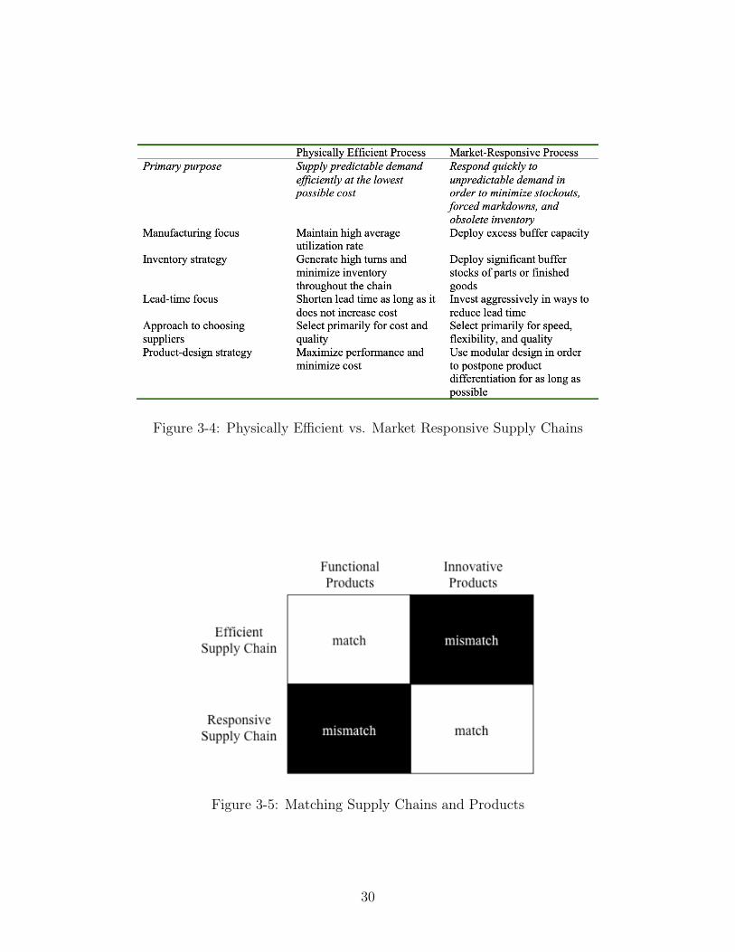
Figure 3-4: Physically Efficient vs. Market Responsive Supply Chains
Figure 3-5: Matching Supply Chains and Products
30

Chapter 4
Sales Velocity and Planogram Space
Relationship
4.1 Motivation
Prior to understanding how any upstream optimization might work, we first needed
to analyze how space is allocated across items and departments. To characterize
the relationship between space allocated for an item and its respective relative sales
velocity, we started with a visualization of absolute number of units sold on the y-axis
and the allocated quantity of items in the planogram1 (POG) for each item in a given
store over a particular month. The question we were trying to answer is if an item
was given four units of space on a shelf (x-axis), how many units of this item were sold
over a particular time-frame (y-axis)? The unit for both axes is item quantity - how
many units were allocated in the POG and how many units were sold. Each graph
was created for a snapshot of one day, thus the y-axis shows how many units were
sold in one day. The last variable required to glean any insight from this analysis
is replenishment accuracy. This metric can be captured as a boolean and defines
whether or not an item was replenished in time to match the sales demand within a
tolerance, or if it was replenished too much or too little. A representative graph is
1A diagram or model that indicates the placement of retail products on shelves in order to
maximize sales. Further detailed in Chapter 2.
31

shown in figure 4-1.
4.2 Methodology
We expected this graph to separate items into three distinct categories based on POG
volume and sales velocity only:
1. Sales velocity greater than space allocation
2. Sales velocity in line with space allocation
3. Sales velocity below space allocation
Figure 4-1: Sales vs. POG Capacity Relationship
In case 1, we expect the item to appear in the left quadrant of the visualization,
above the equality line2. In case 2, we expect items to appear +/- 10% of the equality
line. In case 3, we expect items to appear below the equality line and occupy the
bottom right quadrant of the graph. Case 1 items highlight a strain on in-store labor
since items are selling at faster rates than the space they occupy. Team members are2This is where y=x, units on the POG equals units sold.
32

required to make back room pulls during their shift which takes away from time that
could be spent with guests. Case 2 items define the "sweet spot" of sales demand and
space allocated relationship. These items sell at roughly the same rate as compared
to the space that is allocated. Case 3 items define the slow movers which in some
instances might be occupying more space than is necessary. Ultimately, this visual
raises the question of if space can be shifted to apply more weight to some of the
faster movers that require mid-day restocking, and less weight to some of the slower
movers that have 30x the space for the number of sales they see.
To complete this analysis, we chose a subset of five stores that were all serviced out
of the same distribution center (redacted). Each store was from a different velocity
band (AAA, A, B, C, D)3 - (store names are redacted). These stores were chosen
simply for their designation in each velocity band, no other selection criteria was
employed. Next, we captured sales and POG data for all items in these five stores
during July 2018 and December 2018. The purpose for having these two months
is to compare off-peak and peak seasons. We removed items distributed from food
distribution centers because the POG allocations are generally more fluid and difficult
to monitor due to weighted values. We also removed non-retail items, such as gift
cards, because of how they are positioned in non-POG areas (like racks near the cash
registers). Next, for each subset of data, we took the daily average sales during the
two months in question and plotted against POG capacity.
4.3 Findings
In figure 4-2, we display the outcomes during the off-peak month and in figure 4-3,
we observe the outcomes during the peak month. The breakdown of where items
fall is shown in table 4.1. The dot colors represent the five different store velocities.
The yellow triangle highlights items that fall in case 1. The number of items in this
region is visibly less than the other regions, but are typically the fastest movers like
household essentials (soap, shampoo, paper goods). In comparing the two visuals, the
3More information on store velocity bands in section 2.2.
33

number of items in case 1 increases dramatically during the peak month. The yellow
rectangle highlights items in case 3 that exhibit a small sales to space ratio. The
interesting takeaway here is that the POG capacities do not appear to change, but
the sales velocities do. This signifies that there is potential for further POG volume
optimization that could occur both in off-peak and peak seasons.
Figure 4-2: Off-Peak Sales v POG Analysis
Store Velocity Case 1 (> y=x) Case 2 (Within y=x) Case 3 (< y=x)Off-Peak On-Peak Off-Peak On-Peak Off-Peak On-Peak
AAA 2.2% 3.2% 8.0% 7.4% 89.8% 89.4%A 1.2% 2.0% 7.0% 6.9% 91.8% 91.1%B 1.2% 1.5% 7.3% 6.0% 91.5% 92.5%C 0.9% 1.2% 6.0% 5.4% 93.1% 93.4%D 0.8% 1.2% 5.8% 5.3% 93.5% 93.6%
Table 4.1: Percentage of Items Below, Above, or Within 1:1 Sales to Space Ratio
Now, the question shifts to what impact does this actually have? We know that
the absolute percentage of items that sell more per day than the space that is allocated
is low, so what is the actual impact. To answer this question, we mapped the total
revenue generated within each region as seen in table 4.2. The actual numbers are
redacted but we represent the values as a multiple against the revenue generated by
the items that had parity between POG space and sales volume. While case 1 items
34

Figure 4-3: Peak Sales v POG Analysis
represent approximately 150th of total item volume that case 3 items represent, case 1
items generate 18th the revenue that case 3 items generate. This is largely a function
of the frequency of sale. The analysis further highlights the opportunity to reallocate
POG space towards the case 1 items, which will likely result in less labor time spent
on pulling inventory from backrooms and added sales potential from faster moving
items.
Store Velocity Case 1 (> y=x) Case 2 (Within y=x) Case 3 (< y=x)Off-Peak On-Peak Off-Peak On-Peak Off-Peak On-Peak
AAA 0.6x 1.5x 1.0x 1.0x 6.8x 6.9xA 0.4x 0.9x 1.0x 1.0x 8.0x 9.3xB 0.3x 0.8x 1.0x 1.0x 7.3x 9.8xC 0.3x 0.6x 1.0x 1.0x 9.0x 8.3xD 0.3x 0.5x 1.0x 1.0x 9.9x 8.8x
Table 4.2: Revenue of Items Below, Above, or Within 1:1 Sales to Space Ratio
4.4 Drawbacks and Conclusions
The major drawback of this analysis is the time horizon. The question of time horizon
is crucial, and actually introduces a third variable into this equation - replenishment.
35

If an item is given four units of space, and sells four units at the time of this study,
was it replenished in time to make the next four sales? This is the question that
challenges this analysis. It is more prudent to analyze demand and POG through a
metric that incorporates time, which will be covered in the next chapter.
While Sales v POG is an interesting and important starting point to orient our-
selves with what the data actually means, ultimately, it was not chosen for further
analysis due to a necessity to incorporate a time length for demand explicitly. As
such, we created a more descriptive set of metrics to further our analysis.
36

Chapter 5
Analyzing Inventory Replenishment
5.1 Motivation
In this chapter, we will define metrics that create an accurate representation of Tar-
get’s inventory movement and replenishment strategy. Once we analyze how inventory
is moved, positioned, and stocked, we can begin to discuss optimization. Let us keep
in mind our overall problem formulation:
Determine optimal POG capacity and UOM1 to find efficiency in upstream sortation
(cost varies with different units of measure and replenishment schedules) and down-
stream put-away (including team member productivity influenced by incoming inven-
tory and backroom utilization) without negatively impacting demand signal fulfillment
and customer in-store experience.
The goal here is to balance in-stock and out-of-stock inventory - let us define
the extreme case as a backroom with no inventory. Our model strives to push all
inventory from the truck directly to the sales floor. Of course, this requires perfect
harmony between the following input parameters:
• POG Capacity
• Presentation Minimums1Unit of Measure - refers to size of packaging. Can be an each, store ship pack, vendor case pack,
pallet, etc. Please refer to section 2.2 for more information
37

• Frequency of Replenishment
• Case Pack Quantity
No-Backroom Framework
The "No-Backroom" framework is the basis for all the metrics we define. While
driving backroom inventory to zero is unrealistic in today’s operation, to accomplish
Target’s vision of fulfilling online orders from the backroom, it must be implemented to
some extent in the next five years. Thus, the ideal state of our inventory replenishment
is a model where inventory is directly stocked from truck to sales floor with no leftover
inventory that does not get stocked in the backroom due to spilling over the POG.
There are four key outcomes in generating this model:
• Decreased labor hours in inventory management
• Increased labor availability for guest interaction
• Increased space availability to fulfill online orders
• Decreased overall inventory holding
5.2 Metric Definitions
POG Weeks of Demand (WOD)
The first metric we defined is the POG Weeks of Demand (WOD). This is defined
as the number of weeks over which a full POG could meet all demand, where demand
is taken at a 95% service level2. For example, if we have a shampoo brand that sells
five units per week (at the 95th percentile of demand), and we allocate ten units of
shelf space for the item, the POG WOD for this shampoo is 10 units of space5 sales per week = 2.
2Defines the percentage of times that an item will be in stock given a normal demand distribution.
Mathematically, this is calculated as the number of standard deviations we want to cover from the
mean demand. Based on sales data, we expect that 95% of the time, this item will sell five units or
less per week
38

This metric enables a normalized comparison across departments. Now instead
of merely measuring daily sales against daily POG capacity, we can understand how
many weeks the current POG can last without requiring a replenishment. This is the
solution to the problem we encountered in the Sales vs POG analysis.
Replenishment Spillover
Next, we looked at Replenishment Spillover. This metric defines the percentage
of DPCIs3 that arrived on a particular shipment that did not fit on the POG and
had to be stocked in the backroom. For example, if 20 different DPCIs arrived on a
truck, and after taking all the inventory to the sales floor, it was observed that 10
DPCIs could not fit fully into the POG, the replenishment spillover is1020 , or 50%. To
be classified as spilled over the inventory must simply not fit completely in the space
that is available. This could mean that one unit of the DPCI spilled over, or all the
units of the DPCI spilled over - both cases count as one DPCI spilled over. This
does not mean that 50% of all inventory that came off the truck spilled over into the
backroom, this just means that 50% of the DPCIs on the truck were stocked in the
backroom. The reason for looking at the count of DPCIs individually is because each
individual DPCI requires a unique stocking location in the backroom. If there was1
100 DPCIs that spilled over but that one DPCI comprised 99% of inventory on the
truck, it is less labor effort since the team member must only visit one location in the
backroom. In our example, the team member must visit 10 different locations in the
backroom to complete stocking inventory. An example of this calculation is shown in
figure 5-1.
We take all calculated data and aggregate by department and our sample set of
three stores. In a later analysis, we will look at why items spillover and how we
can optimize our inventory strategy to reduce spillovers, thereby moving us closer to
accomplishing our "No-Backroom" framework.
3DPCI is a unique item identifier that is shorthand for department-class-item. This is inter-
changeable with SKU.
39
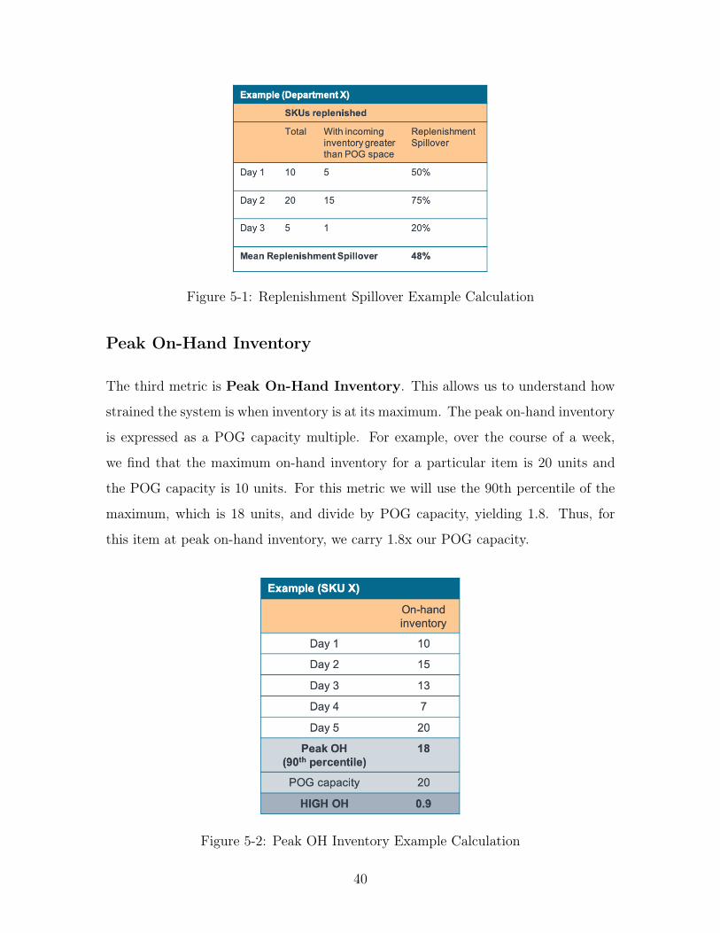
Figure 5-1: Replenishment Spillover Example Calculation
Peak On-Hand Inventory
The third metric is Peak On-Hand Inventory. This allows us to understand how
strained the system is when inventory is at its maximum. The peak on-hand inventory
is expressed as a POG capacity multiple. For example, over the course of a week,
we find that the maximum on-hand inventory for a particular item is 20 units and
the POG capacity is 10 units. For this metric we will use the 90th percentile of the
maximum, which is 18 units, and divide by POG capacity, yielding 1.8. Thus, for
this item at peak on-hand inventory, we carry 1.8x our POG capacity.
Figure 5-2: Peak OH Inventory Example Calculation
40

Similar to the previous metric, we take all calculated data and aggregate by de-
partment and our sample set of three stores. An example of this calculation is shown
in figure 5-2. In our analysis, we will investigate how this metric can be used to
optimize for space.
Backroom Inventory (BRI)
The final metric we analyze is Backroom Inventory (BRI) as a percentage of POG
capacity. Daily backroom inventory is computed by subtracting POG capacity from
total on-hand inventory, assuming that whatever is not on the POG must be in the
backroom. For each DPCI, we take the mean BRI over all days in our data set.
5.3 Applying Metrics to Current Operations
POG Weeks of Demand (WOD)
The results of this calculation can be seen in figure 5-3 and figure 5-4. The major
takeaways are that department level POG WOD varies dramatically across stores,
which could be a result of the varying store velocity bands. The mean across all
stores and departments was 2.0, meaning that on average Target stores can satisfy
about 2 weeks of demand with current POG sizing, assuming the POG was full to
begin with.
In figure 5-4, we have created a violin plot to show the distribution of POG
WOD by DPCI in a select group of departments. The red dots signify outliers. The
departments show major variability across stores – highlighting an opportunity to
optimize replenishment store to store. After accounting for presentation minimums,
the current POG could handle approximately two weeks of demand, which makes
for an interesting segue into our replenishment strategy since most stores receive
inventory multiple times per week.
41

Figure 5-3: POG WOD Calculations
Figure 5-4: POG WOD Calculations - Distributions
One specific example of where this metric sheds light on potential space optimiza-
tion is shown in figure 5-5. The dark green line shows POG capacity for this item at
15 units, On-Hand (OH) inventory hovers around 5 units, the presentation minimum
42

is 3 units, and demand hovers around 1 unit. The POG WOD for this item would
likely be 14.0, meaning the POG could satisfy 14 weeks of demand (given that we see
1 unit sold per week). The question now becomes whether we believe it is prudent
to utilize space in this fashion, or to re-allocate some space to an adjacent item that
might see greater demand.
Figure 5-5: Item Metrics and Inventory over Time
Replenishment Spillover
The Replenishment Spillover metric builds on the POG WOD metric in suggesting
immediate optimization of one of the three critical replenishment variables - POG
Size, Case Pack Quantity, or Replenishment Frequency. We will discuss this in a
later section. From our calculations, shipments regularly spillover to the backroom
across stores and departments. The mean in this study was 48%, meaning that in Q3
and Q4 of 2018, 48% of all shipments to the three stores in our sample sets had at
least one DPCI that did not fit on the POG and was thus backstocked. This result
includes the scenario where there is some inventory on the POG and the scenario
where there is no inventory on the POG, but the incoming inventory pushes the
space utilization over what is allocated. We observe that while this is a consistent
43

problem across stores and departments, the higher velocity store in this study has
a particularly high rate of replenishment spillovers. Ultimately, these occurrences
violate our "No-Backroom" framework but to really understand the impacts to the
day-to-day operation, we look at it from the lens of a team member.
Figure 5-6: Replenishment Spillover Calculations
To understand the real impact of spillovers, we devised an estimate of total team
member time that was spent on backstocking items that did not fit on the POG.
The baseline assumptions are that 2 team members involved in putting away items
after items are offloaded from an incoming truck, the put-away takes 3 hours, and the
estimated time per item touch is 0.05 minutes (3 seconds). With these assumptions
multiplied by the number of items that spilled over, on average backstocking takes 1
hour per team member per shipment, or 33% of total put-away time.
44

Figure 5-7: Hours Spent Per Team Member Backstocking Spillover Units
Now if we dive into departments and stores, we can find the biggest culprits of
spilled over DPCIs. There is certainly a correlation between department and percent-
age of items that do not fit on the POG, but it also appears that the higher velocity
stores receive more inventory on average and require team members to spend 4 hours
(median) taking items that did not fit on the POG to the backroom.
Figure 5-8: Spillover Units by Department and Store
45

Peak On-Hand Inventory
The Peak On-Hand Inventory metric continues our finding of space optimization
potential. It highlights how much the system is strained when we maximize our
inventory holding. As per our findings in figure 5-9, the fast moving inventory (lower
weeks of demand) is over stocked which generates major backroom inventory holding
at peak - this provides another major opportunity to reallocate and optimize space
amongst items. On the y-axis we plot the metric, which is the 90th percentile of
maximum inventory carried during the study period represented as a multiple of
POG WOD. The x-axis is the POG WOD. The meaning of each tick in the box plot
is shown in figure 5-10. In simple terms, the comparison we are observing is for a
given item that has a given POG capacity (measured in weeks of demand for that
item that could be satisfied with the specified POG capacity), when the inventory is
at its highest point, how many times could we fill the POG.
Figure 5-9: Peak OH Inventory vs POG WOD for Three Departments
For an average item in the bath department with a POG WOD of 1, at peak
intervals there is enough inventory to stock this item 1.8x. On the converse, for an
item in the razors department with a POG WOD of 6 (one full POG of this item
could satisfy 6 weeks of demand), at peak intervals there is enough inventory to fill
46

Figure 5-10: Box Plot Tick Mark Explanations
the POG 0.5x. These conditions are highlighted in the red and blue circles. The red
circle denotes DPCIs that force high back room utilization, and egregiously violate our
"No-Backroom" framework. Typically these items are the faster movers, as denoted
by the lower weeks of demand, highlighting the magnitude of safety stock that is
buffered into the system for such items. Any item that falls on the other end of the
spectrum sees unutilized POG space. In our razor example, even at peak times, we
rarely fill the POG. This highlights a clear opportunity to reallocate some space from
DPCIs with higher WOD towards items with lower WOD such that overall backroom
utilization could decrease.
In order to characterize where the lines could be drawn, we have created three
classifications of items through this metric - high, par, and low. Items with Peak OH
>= 1.25 are classified as high, items with Peak OH = 1 are classified as par, and
items with Peak OH <= 0.75 are classified as low. The breakdown by department
for a high velocity store is shown in figure 5-11. The x-axis denotes the percentage of
items in the department that fall into each classification.
This metric could be a starting point of space optimization. Striving for more par
items by department will decrease overall backroom inventory holding.
Backroom Inventory
The Backroom Inventory (BRI) metric captures how many times inventory held
in the backroom could fill up a POG. The inventory in the backroom is calculated as
47

Figure 5-11: Peak OH Distribution by Department
total OH inventory minus POG capacity. While there is a data set that tracks daily
backroom inventory counts, it is dependent on team members accurately scanning in
all inventory. To avoid any manual scanning errors, we choose to calculate it ourselves
with more accurate data sets - POG Capacity and total on hand inventory. If we plot
consolidated department BRI against consolidated department POG WOD, we find
an inverse correlation which is accurate with our past analyses. The departments
that carry less weeks of demand on the POG (either as a function of space available
or how high demand is), tend to over run backroom inventory.
As we see in figure 5-12, the furniture department certainly carries high backroom
inventory, but this is likely due to lack of space available of the main sales floor.
So we do not categorize furniture as a poorly performing department by inventory
holding. Bath and paper and plastic, however, typically hold an extra quarter POG
worth of inventory in the backroom. If we pair this analysis with our previous findings
from peak OH inventory and replenishment spillover, we can see that bath and paper
and plastic have high spillover rates and over half of the items in the departments
are stocked at around 50% greater than what the POG can hold. Either we should
reduce replenishment frequency or increase POG capacity, otherwise we continue to
48

Figure 5-12: Backroom Inventory as a POG Capacity Multiple vs POG WOD
see labor utilization for backstocking and rising backroom inventory.
5.4 Root Cause of Replenishment Spillover
So far, we have defined the metrics needed to analyze and optimize inventory move-
ment and holding at Target. Next, we need to understand which of the courses of
action should be taken. Is inventory spilling over as a result of inaccurate POG siz-
ing, UOM, or replenishment frequency? The way we conceptualize the root cause is
shown below:
1. POG sizing: Our forecast predicted that we would need more units than the
POG could hold.
2. UOM: Our forecast predicted that we would need an additional number of units,
but due to case pack sizing, we received more than needed.
3. Replenishment frequency: Inventory sent in excess of the UOM or POG spillover
units.
To visualize how this would work, we walk through an example in figure 5-13.
Starting from the bottom, this particular item has 2 current on-hand units in store
49

and the POG capacity of the item is 5 units. In this situation, our demand forecast
predicted that we would need an additional 5 units to satisfy demand over the next
interval. With these parameters, we need to hold an inventory of 7 units with a POG
size of 5 meaning 2 units will spillover to the backroom. Thus, POG sizing contributes
2 units of spillover.
Figure 5-13: Example of Replenishment Spillover Root Cause
Now, let us assume the case pack quantity for this item is 4, so the minimum we
receive to meet our demand forecast of 5 is 2 boxes or 8 units. This would bring
our total on hand level to 10 units, meaning 5 units will spillover. We already know
that 2 units are spilling over as a result of POG sizing, thus the remaining 3 units
are spilling over as a result of UOM. Finally, we actually receive 3 boxes, or 12 units.
So our total on hand inventory is 14 units. These last extra 4 units comprise the
replenishment frequency root cause because we simply did not need them, they were
50

just delivered too frequently.
Figure 5-14: Actual Replenishment Spillover Root Cause
After running this methodology on our data set, the final results paint an interest-
ing root cause more holistically. At the higher velocity store, replenishment frequency
is the most frequent culprit for driving backroom inventory. This is followed by POG
size and UOM. The large spillover due to replenishment frequency might suggest
an unreasonably high safety stock or an inaccurate forecast. At the lower velocity
stores, we see a different outcome. Spillover occurs more as a result of POG sizing.
This suggests that shipments happen more rarely, given what we learned in our POG
WOD analysis which showed POGS hold approximately 2 weeks of demand. Thus
items may not be replenished on a frequent basis, but when they are replenished,
shipments come with excess inventory in order to minimize the number of shipments
51

needed. UOM is the third root cause across the board, but appears consistent across
departments and store velocity bands. This suggests a system-wide dynamic UOM -
for example, sending a case pack of 2 to "C" stores versus a case pack of 4 to "AAA"
stores could enable a more lightweight inventory strategy that can be adapted as
demand patterns change.
5.5 Conclusions
Metrics
The final metrics we used to analyze replenishment strategy are:
1. POG weeks of demand (WOD) – how many weeks of demand can an item satisfy
if it was fully stocked on the sales floor.
2. Replenishment spillover – how many items per shipment do not fit on the sales
floor and are transferred to the backroom.
3. Peak on-hand (OH) inventory – maximum quantity of inventory held in the
store over a given time period.
4. Back room inventory (BRI) – amount of inventory carried in the backroom
expressed as a multiple of allocated POG capacity for a given item.
Analysis
First, with POG Weeks of Demand (WOD) we observe that on average, POGs
can meet about 2 weeks of demand - yet we know that we send trucks to every store
at least three times per week. Next, with Replenishment Spillover, we find that
about half the time, team members have to backstock inventory that did not fit on
the POG. This could be a result of sending too much, not having the right amount
of space for the item, or the UOM. In all cases, we estimate that team members use
33% of their time pushing items to the backroom. This is an opportunity cost, not
52

an actual cost, in which team members could spend more time with guests. With
Peak On-Hand Inventory, most items either occupy less than 75% or more than
125% of their allocated POG space at peak inventory intervals. This highlights the
opportunity for POG optimization - taking space that is unused by the slower movers
and shifting it to faster movers in order to reduce backroom inventory. Lastly, with
Backroom Inventory (BRI), the findings are as expected but this metric should
be a barometer as tweaks are made to the system.
53

Chapter 6
Simulating an Optimal Case Pack
Quantity
6.1 Motivation
In this chapter, we will discuss how we developed and executed a computer simula-
tion of how to choose the right optimization strategy in order to decrease backroom
inventory.
Prior to discussing all the variables, there is a major disclaimer to discuss first.
This simulation is done using known demand, thus we are working towards under-
standing the total optimization potential, knowing that due to uncertainty in future
demand, these results will be impossible to achieve in real life. Nonetheless, improv-
ing inventory holding even incrementally can yield tremendous cost savings from a
labor perspective.
6.2 Methodology
Data Collection and Orientation
The objective function of this optimization exercise is to minimize backroom inventory
holistically for a store over a period of time. The variables that we can modify are
54

case pack quantity, replenishment frequency (manifested as the number of cases sent
in a given replenishment), or both. The detailed approach comprised the following
steps. We first created a data model comprising the following elements:
• Inventory on-hand information by day during July 2018. This includes daily
starting and daily ending on-hand inventory counts.
• POG capacity by day during July 2018
• Shipment dates and quantities during July 2018
• Sales information by day during July 2018
We can define backroom inventory with the following equation (all inventory that
does not fit on the POG):
InvBR = InvOH � POG
The inventory available at the end of day t is described by following equation,
where Dt denotes sales demand on day t, At is a boolean denoting whether or not a
shipment arrived, and St denotes the quantity of items that was shipped to the store
on day t:
Invt+1 = Invt �Dt + At ⇤ St
The shipment quantity St can be further broken into the following, where Ct
denotes the number of cases and cpq is the case pack quantity:
St = cpq ⇤ Ct
Bringing all of these equations together yields the following optimization exercise:
min
30X
n=1
InvBRt = [max((Invt �Dt + At ⇤ (cpq ⇤ Ct))� POG), 0]
The following sections describe the optimization process, which most closely re-
sembles gradient descent albeit in a discrete manner. Without changing demand and
replenishment date, we use this equation to modify case pack quantity and number
of cases over the month long timeframe to find which values of cpq and C � t mini-
mize overall backroom inventory holding. We approach this by calculating a gradient
55
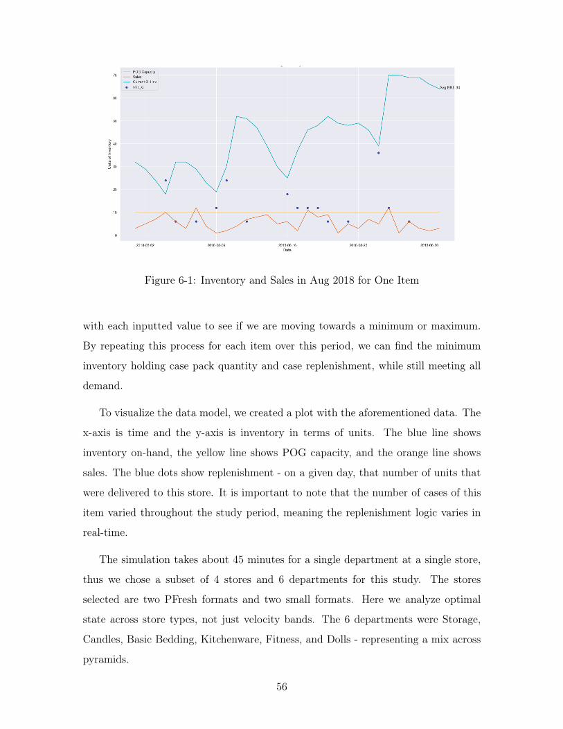
Figure 6-1: Inventory and Sales in Aug 2018 for One Item
with each inputted value to see if we are moving towards a minimum or maximum.
By repeating this process for each item over this period, we can find the minimum
inventory holding case pack quantity and case replenishment, while still meeting all
demand.
To visualize the data model, we created a plot with the aforementioned data. The
x-axis is time and the y-axis is inventory in terms of units. The blue line shows
inventory on-hand, the yellow line shows POG capacity, and the orange line shows
sales. The blue dots show replenishment - on a given day, that number of units that
were delivered to this store. It is important to note that the number of cases of this
item varied throughout the study period, meaning the replenishment logic varies in
real-time.
The simulation takes about 45 minutes for a single department at a single store,
thus we chose a subset of 4 stores and 6 departments for this study. The stores
selected are two PFresh formats and two small formats. Here we analyze optimal
state across store types, not just velocity bands. The 6 departments were Storage,
Candles, Basic Bedding, Kitchenware, Fitness, and Dolls - representing a mix across
pyramids.
56

Case Pack Quantity
Now, we begin with optimizing for case pack quantity. First, we calculated post-
shipment inventory levels by taking the ending on-hand inventory from the day be-
fore a shipment arrived and adding the number of units that came in that ship-
ment, by multiplying case pack quantity by number of cases. If this value exceeded
the POG capacity, a boolean column tracking specifically this case pack quantity
(named "cpq_5_bri" for example) was set to True for generating backroom inven-
tory. Another column is created for this particular case pack quantity (column name
is "cpq_5_bri_q" for example) populated with the units of backroom inventory that
was generated by this case pack quantity. In addition, the total sales count was
summed until the next shipment to calculate a boolean of whether or not this post-
shipment quantity could satisfy all sales until the next shipment. This value is added
to another new column ("cpq_5_meet_demand" for example). Note, in this first
step where we optimize for case pack quantity, we assume the replenishment engine
would have sent the same number of cases. This process is repeated with a range of
case pack quantities starting from an each to 2x what the current case pack is.
Replenishment Frequency
Next, to simulate an optimal replenishment frequency, we use today’s case pack quan-
tity and run a similar analysis but instead of holding the number of cases that are
sent constant, we modify this value to the bare minimum needed to satisfy demand
until the next shipment. In some cases, this value can be set to zero if no additional
cases are needed. This function is only run once, as there is only one use case.
Case Pack Quantity and Replenishment Frequency
With this information, we now have which case pack quantity will generate the least
amount of backroom inventory and still satisfy all demand, as well as an inventory
count if we sent less inventory overall. Lastly, we run a combination of both simula-
tions - what would happen if we used the optimal case pack quantity but only sent
57

the bare minimum number of cases to cover a 95% service level and all presentation
minimums?
6.3 Findings and Results
The output of this simulation yields the lowest possible backroom inventory holding
on average during the study period for an individual item at a particular store. We
run the simulation for all items in our subset of departments at all of the selected
stores. The outputted data informs us of how much inventory we hold today for these
departments by store, and also what the optimal state would be. Another captured
data point is the unit of measure (UOM) - each, SSP, VCP, or pallet1. If the optimal
case pack quantity is different from current state, then we also adjust the optimal
UOM.
Figure 6-2: Full Simulation of Optimized Inventory State
Prior to looking at the summary results, let us start by analyzing the outcomes
for the same item we plotted in earlier in this chapter. We still observe the current
state, represented by the blue line, which generates a daily average of 34 units in the
backroom. This is with a case pack quantity of 6 units. Next, our first simulation1Chapter 2.2 details the different units of measure.
58

method, drawn in blue, found that a case pack quantity of 5 units could lower average
daily backroom inventory to 16 units. If we sent inventory at the correct frequency
with our current case pack quantity, drawn in magenta, backroom inventory would
drop to a daily average of 8 units. And finally, the combination simulation, if we
did both a case pack of 5 units at an optimal replenishment frequency, we would see
backroom inventory drop to 6 units per day, an 82% reduction in backroom inventory
holding with no missed sales. The following 4 graphs highlight the difference in UOM
across our 6 department.
At the high velocity PFresh, the current to optimal state shift suggests reducing
the full case mix from 55% to 42% and the SSP mix from 24% to 17% while increasing
eaches from 21% to 41%. This conclusion is in line with our previous findings that the
faster moving stores see excessive replenishment. By reducing the case pack quantity
to one (otherwise known as an each), we would reduce the gross inventory arriving
at a store, and as this analysis shows, reduce backroom inventory by 42%.
Figure 6-3: High Velocity PFresh Optimal UOM for 6 Departments
At the high velocity small format store, the current to optimal state shift suggests
reducing the full case mix from 50% to 43% and the SSP mix from 26% to 23% while
increasing eaches from 24% to 34%. T-2799 is a small format store that likely already
receives a high percentage of items in each format, thus the differences here are in-
line with what we would expect and in comparison to a PFresh format. Ultimately
59

backroom inventory decreases by 41%.
Figure 6-4: High Velocity Small Format Optimal UOM for 6 Departments
At the medium velocity small format store, the current to optimal state shift
suggests reducing the full case mix from 38% to 33% while increasing eaches from 33%
to 38%. Of all the stores we analyzed, this one appeared to receive inventory relatively
close to the optimal state, which would show a backroom inventory reduction of 48%
for our 6 department sample set.
Figure 6-5: Medium Velocity Small Format Optimal UOM for 6 Departments
At the medium velocity PFresh, the current to optimal state shift suggests re-
60

ducing the full case mix from 52% to 46% while increasing eaches from 26% to 34%.
Similar to the medium velocity small format, the optimal state is not a large shift
from today’s operations, but could help to reduce backroom inventory by 43%.
Figure 6-6: Medium Velocity PFresh Optimal UOM for 6 Departments
Overall, our sample set shows promise through this simulation and there is an op-
portunity to reduce backroom inventory by roughly 45% when considering this model.
Our final graphic aggregates this data and shows current state UOM breakdown in
gray and optimal state UOM breakdown in green.
Figure 6-7: All Stores Current vs Optimal UOM
61

Chapter 7
Conclusions and Future Research
7.1 Key Research Findings
This thesis proposed that an optimal "unit of measure" (UOM) and replenishment
schedule in upstream sortation will highlight current inefficiencies with POG siz-
ing and optimize for downstream labor cost without negatively impacting critical
functions of the store, including demand signal fulfillment and the customer in-store
experience (quantified as stock-outs). Theses studies support this hypothesis.
First, we created a classification model to understand how space is utilized relative
to revenue. This model proved to be inconclusive due to the necessity of incorporating
a time element.
Next, we established four key metrics, POG Weeks of Demand (WOD), Re-
plenishment Spillover, Peak On-Hand (OH) Inventory and Backroom In-
ventory (BRI), to analyze current operations and set the baseline for any opti-
mization exercises. The POG WOD metric reveals how much demand Target could
satisfy with a full POG. The Replenishment Spillover metric shows that 48% of
all shipments have an item that must be stocked in the backroom. The Peak OH
Inventory metric shows that there is a large discrepancy in space utilization between
fast moving inventory - over utilization of space - and the slow moving inventory -
under utilization of space, leaving a large gap that could be closed by shifting space
from slow movers to fast movers. Finally, the BRI metric shows how much inventory
62

is carried in the backroom as a multiple of POG capacity by department. Through
these metrics, we were also able to classify the root causes for inventory spilling over
from the sales floor into the backroom which violates our goal, the "No-Backroom"
framework. These root causes were UOM, POG size, and replenishment frequency,
with the largest culprit varying depending on which velocity band the store is in.
AAA stores have spillover largely due to replenishment frequency, whereas D stores
have spillover largely due to POG size.
In the final study, we simulated what would happen to backroom inventory if we
had optimal UOM and optimal replenishment frequency. Across the board, an opti-
mization of UOM combined with replenishment frequency yields the most compelling
results - generally showing a backroom inventory decrease of >40% across multiple
store types.
7.2 Recommendations for Target
The outcomes reveal a large opportunity to optimize inventory holding along three
axes - UOM, POG sizing, and replenishment frequency.
This study helped to set the stage for a larger scale optimization exercise. The
next step should dive into building a business case for optimization through deeper
cost modeling, by extrapolating our labor estimations and using actual time study
data. This will enable, what we believe is, a mutually agreed upon supply chain
savings metric - labor hours.
To make this a reality, we would need to look at:
1. Cost of labor and supply of labor by store, by time.
2. Labor capacity of a worker, considering different activities to be performed.
3. Impact of assortment carried and replenishment strategy (timing and sortation)
on labor.
The data could be pulled from the labor schedule by store (staffing level, shift
63

timing) and labor metrics by team member (time taken to put-away an item, time
taken to pack a ship from store order).
With this information, it makes sense to begin a small scale test comprising one
department at one store and manipulating UOM and frequency to see how backroom
inventory holding changes and how team members change their day-to-day tasks. Of
course, working with Merchandising and Stores stakeholders. From here, it would
make sense to scale the study to more departments and stores, and begin engaging
the POG sizing exercise.
7.3 Opportunities for Future Research
In future research there are some key areas to consider. First, it would be prudent
to continuously iterate and improve the metrics detailed in this study, either how
they are calculated (from a statistical point of view) or how the data is collected.
This solution architecture will ultimately help Target quantify the longstanding pain
points in Supply Chain.
Next, a cost per unit model will enable the expansion of this model. There is
work on this already, but we believe this will be a crucial step to optimizing UOM,
regardless of whether the store is replenishing an item on the POG or fulfilling an
online order via ship from store. The data needed to build a cost analysis for this
model is handling and shipping costs from store by item (ship from store process
path), handling and shipping costs for online orders from fulfillment centers, inventory
storage costs at distribution centers, fulfillment stores, and in backrooms by item,
costs by item shipment type (pallet, case, each, breakpack) from the distribution
center to the store, and all labor related (sorting, stowing, picking) costs in the
distribution center by item.
Lastly, there is an opportunity to study SKU rationalization. Target could likely
carry narrower assortments (either item type or quantity) while maintaining perfor-
mance metrics, including customer experience and presentation minimums. This is
a tricky phenomenon to study given that the assortment offered can significantly
64

influence demand forecasts.
7.4 Closing Remarks
While this study sheds light on some of the major optimization opportunities for
inventory movement at Target, there are still other factors that must be considered
in more depth such as demand forecasting (for example, why are the levers set to
their existing levels such that we send three cases when we really needed two?), labor
productivity (what would be the broader effects of reducing backstocking in stores?),
transportation (it is unlikely that less inventory replenishment as suggested by this
study would mean that Target will send less trucks out, ultimately the available
space will be filled by other inventory), and vendor relations (is changing the case
pack quantity a feasible exercise?).
Nonetheless, we believe this to be a great starting point to help Target make
more informed inventory decisions, find high ROI inventory optimization efforts, and
continue to enhance the way consumers perceive and interact with the big-box retail
industry.
65

Appendix A
Terminology
• Backroom: storage space in the back of most stores. It varies in cubic volume
from store to store.
• Backroom Pulls: when a team member has to go to the backroom to pull
inventory to the sales floor.
• Backstocking: the act of moving inventory to the backroom and scanning it
in to ensure system accuracy.
• DPCI: the item hierarchy pattern at Target. Shorthand for department-class-
item identifier.
• First Pass Yield: when inventory goes straight from the truck to the sales
floor and is not backstocked.
• Guest: how customers are named at Target. This helping to build the brand
around how team members should interact with the people walking through the
door.
• Peak: time frame surrounding Q4 of the calendar year. This is generally when
retail industry sees a major spike due to consumer behavior changing around
the holiday season.
66

• Planogram (POG): a diagram or model that indicates the placement of retail
products on shelves in order to maximize sales.
• Sales Floor: the "front" of the store where guests can walk through aisles and
make purchases at the front cashier registers.
• Sales Velocity: measure of how quickly items are sold off the shelves, typically
quantified in sales per unit time (day, week, month, quarter).
• Space Allocation: how much cubic volume is given to a certain item. This is a
result of negotiations with vendors, brand strategy, and overall Target strategy
to build an assortment mix with varying quantities of options for guests.
• Unit of Measure (UOM): the type of vessel an item is transported in.
• Velocity Band: groupings of stores that fall into different revenue ranges. For
example, the highest revenue generating stores in the network are known as
"AAA" stores, whereas the least revenue generating stores are known as "D"
stores. Other options in order are A, B, and C.
67

Bibliography
[1] V Trauzettel A Erceg. Packaging in retail supply chains. Business Logistics inModern Management, University of Osijek, Croatia, October 2016.
[2] Ali Aouad, Vivek Farias, Retsef Levi. Assortment optimization under consider-then-choose choice models. SSRN, 2015.
[3] Ali Aouad, Vivek Farias, Retsef Levi, Danny Segev. The approximability ofassortment optimization under ranking preferences. Operations Research, 2018.
[4] Ronald Ballou. Improving the physical layout of merchandise in warehouses.Journal of Marketing, 31:60, 07 1967.
[5] C. Klappich, Rick Franzosa, Simon Tunstall, Tim Payne.Predicts 2020: Supply Chain Technology, December 2019.https://www.gartner.com/document/3975870.
[6] Marshall Fisher. What is the right supply chain for your product? HarvardBusiness Review, 1997.
[7] Guenov, M., Raeside, R. Zone shapes in class based storage and multicommandorder picking when storage/retrieval machines are used. European Journal ofOperational Research, 92:37–47, 1992.
[8] J. L. Heskett. Putting the cube-per-order index to work in warehouse layout,volume 4, pages 23–30. Transportation and Distribution Management, 1964.
[9] Jim Blaeser, Marc Iampieri and Roshan Varma. Top trend in shipping? Moreconsumers want fast and free, 2018. https://emarketing.alixpartners.com.
[10] Steven T. Hackman John J. Bartholdi III. Warehouse and Distribution Science.Georgia Tech, 2019.
[11] Carl Kallina. Application of the cube-per-order index rule for stock location ina distribution warehouse. INFORMS Journal on Applied Analytics, 11 1976.
[12] L. B. Schwarz, W. H. Hausman and S. C. Graves. Optimal storage assignmentin automatic warehousing systems. Management Science, 22(6):629–638, 1976.
[13] Martin Joerss, Jurgen Schroder, Florian Nehaus. Parcel delivery - the future oflast mile. McKinsey Global Institute, 2016.
68

[14] F.L. Neal. Controlling warehouse handling costs by means of stock location audits,pages 31–33. Transportation and Distribution Management, 1962.
[15] Nitin Chaturvedi, Mirko Martich, Brian Ruwadi, Nursen Ulker. The future ofretail supply chains. McKinsey Global Institute, 2016.
[16] Croucher P. Rushton, A. and P. Baker. The Handbook of Logistics and Distribu-tion Management: understanding the supply chain. Kogan Page, 2014.
[17] Jia Wertz. 5 trends that will redefine retail in 2019, 2018.https://www.forbes.com.
69