Assessing the Biological Condition of Florida Lakes:

Development of the Lake Vegetation Index (LVI)

Final Report

Prepared for:

Florida Department of Environmental Protection Twin Towers Office Building

2600 Blair Stone Road Tallahassee, FL 32399-2400

Leska S. Fore*, Russel Frydenborg**, Nijole Wellendorf**, Julie Espy**,

Tom Frick**, David Whiting**, Joy Jackson**, and Jessica Patronis**

* Statistical Design 136 NW 40th St.

Seattle, WA 98107

** Florida Department of Environmental Protection 2600 Blair Stone Rd.

Tallahassee, FL 32399-2400

December, 2007

ii

This project and the preparation of this report was funded by a Section 319 Nonpoint Source Management Program Implementation grant from the U.S. Environmental Protection Agency through an agreement with the Nonpoint Source Management Section of the Florida Department of Environmental Protection. The cost of the project was $54,600, which was provided entirely by the U.S. Environmental Protection Agency.

iii

TABLE OF CONTENTS

Table of Contents....................................................................................................................... iii

List of Tables .............................................................................................................................. v

List of Figures ............................................................................................................................ iv

List of Appendices ..................................................................................................................... vi

Acknowledgments..................................................................................................................... vii

Foreword .................................................................................................................................. viii

Abstract ....................................................................................................................................... 1

Introduction................................................................................................................................. 3

Methods....................................................................................................................................... 5

Study area................................................................................................................................ 5

Lake sampling......................................................................................................................... 6

Quantifying human disturbance.............................................................................................. 8

Metric development and testing............................................................................................ 11

Sensitive and tolerant taxa evaluation................................................................................... 14

Lake Vegetation Index (LVI) development and testing ....................................................... 15

Expectations for statistical correlation.................................................................................. 18

Results....................................................................................................................................... 20

Human disturbance gradient ................................................................................................. 20

Metric selection..................................................................................................................... 21

Sensitive and tolerant taxa .................................................................................................... 31

Evaluation of the Lake Vegetation Index (LVI) ................................................................... 33

Correlation of LVI with human disturbance and natural features ................................... 34

Variability analysis of alternative lake sampling protocols ............................................. 35

Metric scoring for the LVI ................................................................................................ 40

Validation of the LVI with independent data .................................................................... 41

Description of outliers ...................................................................................................... 42

iv

Comparison of spring and summer LVI values................................................................. 44

Discussion................................................................................................................................. 46

Human disturbance gradient ................................................................................................. 46

Biological indicators ............................................................................................................. 47

Statistical precision of the Lake Vegetation Index (LVI)..................................................... 48

Recommendations..................................................................................................................... 50

Conclusions............................................................................................................................... 53

References................................................................................................................................. 54

v

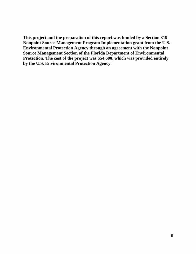
LIST OF TABLES

Table 1. Scoring rules for HDG.....................................................................................................10

Table 2. Examples of LDI coefficient values ................................................................................11

Table 3. Coefficient of conservatism (CC) scoring criteria ..........................................................13

Table 4. Correlation for HDG and its component measures..........................................................20

Table 5. Comparison of water chemistry measures for porous and non-porous soils ...................21

Table 6. Candidate plant metrics and their correlation with HDG, WQ index, LDI, and habitat index...............................................................................................................................................23

Table 7. Plant taxa most frequently identified as dominant ..........................................................25

Table 8. Plant taxa that were significantly associated with low or high HDG ..............................32

Table 9. Correlation between LVI, measures of disturbance, and natural features .......................34

Table 10. Coefficients from multiple regression for LVI and its component metrics...................35

Table 11. Cumulative number of taxa for 12 lake sections ...........................................................36

Table 12. Variance estimates and number of detectable categories for LVI .................................37

Table 13. Correlation between LVI, its component metrics and HDG for different sampling methods ..........................................................................................................................................39

Table 14. Correlation between LVI and measures of disturbance for different numbers of replicate LVI samples ....................................................................................................................40

Table 15. Metric scoring rules for LVI..........................................................................................41

Table 16. Correlation between LVI and measures of disturbance for the validation data set .......42

Table 17. Lakes with higher or lower LVI values than predicted by HDG...................................43

vi

LIST OF FIGURES

Figure 1. Diagram showing 12 lake sampling sections ...................................................................7

Figure 2. Detail of lake section sampling methods..........................................................................8

Figure 3. LVI plant metrics plotted against HDG..........................................................................27

Figure 4. LVI plant metrics plotted against the WQ index............................................................28

Figure 5. LVI plant metrics plotted against the habitat index........................................................29

Figure 6. LVI plant metrics plotted against LDI............................................................................30

Figure 7. Plant CC value plotted against the average HDG for lakes in which taxon was found .33

Figure 8. Species accumulation curve for lake sections ................................................................36

Figure 9. Number of categories that LVI could detect for different sampling protocols ..............38

Figure 10. Distribution of LVI values............................................................................................39

Figure 11. LVI plotted against HDG for the validation data set....................................................42

Figure 12. LVI plotted against HDG with outliers indicated.........................................................43

Figure 13. LVI for repeat visits during spring and summer for 15 lake sites ................................45

Figure 14. Diagram showing recommended lake sampling for LVI .............................................50

LIST OF APPENDICES

Appendix 1. Aquatic plant attributes

Appendix 2. EPA’s wetland plant attributes

Appendix 3. Results of testing for tolerance and sensitivity

Appendix 4. LVI values by district

Appendix 5. Additional tables

Appendix 6. LVI validation and calibration for 2005–2006 sampling

Appendix 7. Biological condition gradient to define biocriteria for LVI

vii

ACKNOWLEDGMENTS

Florida Department of Environmental Protection (DEP) biologists provided comments and

guidance throughout the development and testing of the lake vegetation index. Data organization

and retrievals, explanation of Florida DEP field and laboratory methods, and general discussions

of plant biology and lake management were provided by E. McCarron, D. Miller, A. O’Neal, and

A. Wheeler. E. McCarron and D. Cobb provided administrative support and a regulatory

perspective. Biologists throughout Florida collected and identified macrophyte samples,

including L. Banks, F. Butera, T. Deck, D. Denson, J. Espy, K. Espy, S. Evans, T. Frick, R.

Frydenborg, S. Gerardi, M. Heyn, J. Jackson, T. Kallemyen, P. Morgan, P. O’Conner, A. O'Neal,

E. Pluchino, D. Ray, J. Richardson, B. Rutter, D. Scharr, E. Springer, C. Swanson, M.

Szafraniec, R. Taylor, M. Thompson, F. Walton, N. Wellendorf, and A. Wheeler. J. Tobe, D.

Hall, and J. Burkhalter helped with plant identifications. We thank the Florida DEP Integrated

Water Resource Monitoring program for data used to calculate the human disturbance gradient.

viii

FOREWORD

The original version of this document was completed in 2005. Two appendices were added in

2007 that respond specifically to recommendations made in the 2005 version of this report.

Appendix 6 provides additional validation of the association between the biological condition of

lake macrophytes and independent measures of human disturbance using data collected in 2005–

2006. Scoring rules for combining metrics in the lake vegetation index (LVI) were also amended

slightly for this more recent, larger data set. In addition, new estimates of variance for the LVI

were calculated for multiple years of sampling. Appendix 7 describes the development of

biological criteria as part of Florida’s water quality standards for lakes. Recent guidance from the

U.S. Environmental Protection Agency was used to define thresholds for impaired and

exceptional lake condition based on the advice of a panel of regional experts.

1

ABSTRACT

The Florida Department of Environmental Protection (DEP) is required under the Clean Water

Act to assess the biological condition of its streams, rivers and lakes. We developed a

multimetric index, the Lake Vegetation Index (LVI), to assess the biological condition of aquatic

plant communities in Florida lakes. For the development and testing of the LVI, aquatic plants in

95 lakes were sampled by boat during 2000–03. To validate the results for the LVI, data from an

additional 63 lakes were collected in 2004; these data included 15 lakes with repeat visits for

spring and summer. A total of 48 candidate metrics based on measures of community structure,

taxa richness, and percent of total taxa were calculated and tested against independent measures

of human disturbance. An additional 17 metrics derived from plant information from a national

database were also evaluated. To test metrics, we developed a human disturbance gradient

(HDG) that summarized measures of water chemistry, habitat condition, intensity of land use in a

100 m buffer around the lake, and hydrologic modifications. A total of 10 metrics met the

targeted values for correlation with HDG; of these ten, four were not redundant with each other

and were included in the LVI: percent native taxa, percent invasive taxa, percent sensitive taxa,

and the average tolerance value of the taxon present over the largest area.

Tolerant and sensitive taxa were defined based on designations made by 10 expert

botanists working independently to define coefficient of conservatism (CC) scores for wetland

(not lake) plants in Florida. Metrics derived from CC scores were highly correlated with HDG.

In contrast, relatively few individual taxa were significantly associated with HDG: only 29 out of

404 taxa showed significant preferences. Rare taxa were partially to blame for weak results,

more than half of the taxa were found in less than 5 lakes.

Lakes were divied into 12 pie-shaped sections. Plant data were collected from each

section and taxa lists from the 12 sections were kept separate. Using the replicate data, we

compared the ability of different sampling protocols to detect differences in lake condition.

Based on LVI calculated and averaged from four lake sections, LVI could detect five categories

of biological condition.

2

LVI was highly correlated with HDG and other independent measures of human

disturbance for both the development and the validation data sets (-0.68 and -0.72, Spearman’s

r). For the 15 lakes with repeat visits, LVI values for repeat visits within the year were more

variable than for repeat visits on the same-day; however, neither spring nor summer LVI values

were consistently higher across lakes. We conclude that LVI is a reliable indicator of lake

condition and has sufficient statistical precision to detect multiple levels of biological condition.

Given the relatively small data sets available for this study (<200 site-visits), we recommend that

future studies be designed to evaluate the influence of season on metric values, to determine

whether regional adjustments are needed to metric scoring, and to assess the annual variability of

LVI.

3

INTRODUCTION

A primary objective of the federal Clean Water Act (CWA) is “to restore and maintain the

chemical, physical, and biological integrity of the Nation’s waters.” Under the CWA, each state

must develop water quality standards for all its surface waters. Water quality standards include

designated uses assigned to a water body, water quality criteria to protect the uses, and an

antidegradation policy (Ransel, 1995; Karr et al., 2000). Until the late 1980s, most states used

primarily chemical criteria to assess surface waters. A shift occurred when resource managers

realized that chemical criteria alone often fail to protect aquatic life uses (Karr and Chu, 1999).

At that time, EPA recommended that states adopt biological criteria for the protection of water

resources (Karr, 1991).

The state of Florida recognizes the importance of biological monitoring of water

resources and has developed sampling protocols to assess the condition of streams, lakes, and

wetlands based on their biological assemblages (Barbour et al., 1996; Gerritsen and White, 1997;

McCarron and Frydenborg, 1997; Fore, 2004; Lane et al., 2004; Reiss and Brown, 2005). Florida

Department of Environmental Protection (DEP) uses bioassessments derived from these

protocols to define acceptable conditions for the support of aquatic life uses. Within the context

of the CWA, bioassessments can be used to define impairment, evaluate best management

practices, develop targets for management plans or restoration, or identify exceptional resources

for protection (Yoder and Rankin, 1998; Karr and Yoder, 2004).

Compared to rivers, streams, and wetlands, relatively less work has been done to develop

biological monitoring tools for lakes (USEPA, 2002a, 2002b; but see Whittier et al., 2002 and

Harig and Bain, 1998 for lake indicator development). While most states have biological

assessment programs in place for rivers and streams, Florida is one of only nine states with lake

or reservoir bioassessment programs in place and one of only three that is developing numeric

biocriteria for lakes (Gerritsen and White, 1997; USEPA, 2003). In many states, lakes may

represent a smaller proportion of surface waters; however, with more than 7700 lakes greater

than 10 acres in size, lakes represent a significant natural resource in Florida.

4

Although lakes are not wetlands, they share many of the same habitats and taxa within a

particular region. The U.S. Environmental Protection Agency (EPA) has recently supported

numerous research efforts related to the development of bioassessment and biocriteria for

wetlands (USEPA, 2002b). Resources developed for wetland assessment were borrowed and

applied for this study of lakes. For example, extensive literature surveys have documented the

current science for wetland monitoring at the national level (Adamus et al., 2001) and

specifically for Florida (Doherty et al., 2000). Documents published by EPA summarize the

aquatic plant metrics that have been successfully applied in wetlands throughout the U.S., and

this information was very helpful in identifying potential metrics for this study (USEPA, 2002c).

Similar lists of candidate metrics for aquatic plants in lakes have not been developed (Gerritsen

et al., 1998). Another source for potential metrics was Ohio EPA which has tested several types

of plant metrics for inclusion in their vegetation IBIs for wetlands (Mack, 2004). Within Florida,

the multimetric indices developed for isolated depressional herbaceous wetlands by Lane et al.

(2004) and for isolated depressional forested wetlands by Reiss and Brown (2005) included

additional metrics that were tested in this study for lakes. Finally, a study by Cohen et al. (2004)

used the professional experience of ten botanists to define aquatic plant tolerance and sensitivity

to disturbance in wetlands. We used these designations to define sensitive and tolerant plant taxa.

The purpose of this study was to develop a monitoring and assessment tool for lakes

based on aquatic plant sampling. Though used extensively in wetland monitoring, aquatic plants

are rarely selected as indicators of lake condition (but see Nichols et al., 2000 for a Wisconsin

index). Aquatic plants provide an effective endpoint for monitoring lake condition for several

reasons: 1) a wide array of plants with a variety of life history strategies are represented in

Florida lakes, 2) much is known about the specific preferences and tolerances of many of these

plants, and 3) collecting and identifying plants in the field is relatively straightforward, which

means that laboratory costs are minimal. The goals of this study were to identify potential

metrics for aquatic plants, test them against an independent gradient of human disturbance,

combine the metrics into a lake vegetation index (LVI), and determine the most efficient method

for collecting plant data to calculate the index.

5

METHODS

Study area

The state of Florida can be divided into three geographic regions based on watershed drainage

patterns: the northern panhandle, the southern peninsula, and a transition region known as the

northeast. These three regions were used to develop and test a multimetric index for invertebrates

because different species assemblages were associated with these three geographic areas

(Barbour et al., 1996; Fore, 2004). Sufficient data did not exist for lake plants to perform a

similar test for associations between geographic areas and plant species assemblages;

consequently, we used the geographic areas derived from watershed drainage patterns to test for

regional differences in metric values.

The middle and lower Suwannee basin provides a natural demarcation between the

panhandle and peninsula, with the northeast region straddling the upper Suwannee northeast of

the Cody escarpment (White, 1970). Terrestrial vegetation communities in the panhandle

generally consist of mixed pine/oak/hickory forests (Pinus spp., Quercus spp., Carya spp.),

longleaf pine forests (Pinus palustris), hardwood forests with beech/magnolia climax community

(Fagus grandiflora/Magnolia grandiflora), and swamp hardwood forests of cypress (Taxodium

spp.) or tupelo (Nyssa spp.), interspersed by a mosaic of pine plantations, cropland (e.g., corn,

soy beans, peanuts), and pasture (SWCS, 1989; Fernald and Purdum, 1992). The panhandle is

less densely populated by humans than the other areas.

The peninsula has a sandy highland ridge extending down its center almost to Lake

Okeechobee. The elevation of the central ridge is approximately 150 to 200 ft. Terrestrial

vegetation communities on the ridge of the peninsula consist of longleaf pine/turkey oak forests

(Pinus palustris/Quercus laevis), on flat areas are slash pine (Pinus eliottii) or loblolly pine

(Pinus teada) with palmetto/gallberry understory (Serenoa repens/Ilex glabra), and in

depressional areas are marsh/wet prairies (maidencane, pickerel weed), and hardwood wetlands

of sweetbay (Magnolia virginiana), cypress (Taxodium spp.), and ash (Fraxinus spp.; SWCS,

1989). The dominant land use is pasture, cropland (e.g., watermelons, nursery products,

6

tomatoes), and urban areas (Fernald and Purdum, 1992). Dense population centers are located at

Tampa and Orlando.

The northeast region includes portions of the Okeefenokee Swamp, parts of the upper

Suwannee drainage, the Black Creek drainage, and the Sea Island flatwoods. Plant communities

consist of longleaf pine/turkey oak (Pinus palustris/Quercus laevi) on the sandy uplands,

hardwood wetlands of cypress (Taxodium spp.), tupelo (Nyssa spp.), and loblolly bay (Gordonia

lasianthus), pine flatwoods, and marsh (FNAI, 1990). Jacksonville is the only major population

center.

Lake sampling

For this study, lakes were defined as fresh water bodies with >= 2 acres of open water of

sufficient depth and size to require a boat for sampling. Two different data sets were used to

develop and validate the LVI. The first data set included data from 95 lakes that were selected to

represent a broad range of site conditions and human influence across the state. These lakes were

used to test metrics and develop the LVI. Lakes were sampled by Florida DEP during August–

November, 2000–2003. Of the 95 lakes, 17 were located in the panhandle region, 74 in the

peninsula, and 4 in the northeast. Lake surface area was known for 80 lakes and ranged from 8–

3500 acres, with a mean area of 343 acres. Lakes were not selected randomly, nor were they

selected to ensure coverage in all ecoregions. Consequently some geographic areas were not

included.

The second data set included data from 63 additional lakes, and these data were used to

validate the correlation between LVI and independent measures of human disturbance. These

lakes were sampled during March–September, 2004; 34 lakes were located in the panhandle and

29 in the peninsula. Of these lakes, 15 small lakes from the panhandle were sampled during

spring and summer and were used to test for seasonal differences in LVI.

Aquatic macrophytes include aquatic plants large enough to be easily seen by the unaided

eye, as well as some larger algae such as Nitella and Chara. Aquatic macrophytes grow in water

or wet areas and may be rooted in the sediment or floating on the water’s surface. Most aquatic

macrophytes are vascular plants and include herbaceous species as well as trees and shrubs.

7

Each lake was sampled 12 times by dividing the lake into 12 approximately wedge-

shaped sections, depending on the shape of the lake (Figure 1). Within each section, two methods

were used to identify plants: 1) from the boat, plants were identified, using either binoculars or

the unaided eye, while boating slowly along the shore, and 2) plants were also identified within a

5 m belt transect. The transect was perpendicular to the shore, from the mean high water mark

towards the center of the lake. For the belt transect, visible plants were identified and submersed

plants were also sampled with a standard frotus, a device used to collect underwater plants. The

frotus was deployed 5 times along each 5 m belt transect (Figure 2). Lakes sampled before the

fall of 2003 used only the drive-by method (35 of the 95 lakes in the development data set),

while lakes sampled during or after fall 2003 used both methods. Plants identified using the two

above methods were combined into a single taxa list, one for each of the 12 sections.

The plant judged to have the greatest areal extent, determined visually, within each of the

12 lake sections was denoted as “dominant,” while all others were recorded as “present.” If two

taxa were more abundant than the other plants present, they were noted as “co-dominant.” If the

degree of dominance was not readily determined, all plants in the sampling unit would simply be

marked “present.” Plants were identified to the lowest taxonomic level possible, typically

species. Unknown species were placed on ice and sent to an expert for identification.

Figure 1. Diagram showing the method used to divide a typical lake into 12 sections for replicate sampling.

11 12 1 2

3

4

56 78

9

10

8

Emergent Zone

Submersed Zone

Frodus deployment

5 m Belt Transect

Drive-by

Figure 2. Detail of sampling methods used to identify plant taxa within a lake section.

Quantifying human disturbance

Karr and colleagues describe five factors to summarize the ways in which humans alter and

degrade rivers and streams (Karr et al., 1986; Karr et al., 2000). The five factors are flow regime,

physical habitat structure, water quality, energy source, and biological interactions. For this study

data were available to evaluate three of these factors (water quality, physical habitat structure,

and flow regime), as well as human disturbance at the watershed scale.

To evaluate lake water chemistry, DEP biologists measured conductivity, total Kjeldahl

nitrogen (TKN), nitrites/nitrates (NOx), total phosphorus (TP), and algal growth potential (AGP).

We summarized information from these five measures into a water quality (WQ) index by

converting values for each measure into unit-less scores and then averaging the scores. To

convert to unit-less scores, we used the percentiles from a statewide data set (Integrated Water

Resource Monitoring [IWRM] Cycle 1, 2000-2003) to define expectations. For the IWRM Cycle

1 study, water chemistry data were collected from ~1100 randomly chosen lakes. If the observed

9

value from the LVI index development data set was less than the 10th percentile value observed

for the statewide IWRM data set, the lake-visit received a score of 1 for that chemistry measure;

if less than the 20th percentile the lake-visit scored a 2; and so on. We repeated this process for

each of the five chemical measures. After scoring each of the measures, we averaged the unit-

less scores (ignoring missing data) for all the chemical measures to define the water quality

(WQ) index. For the 95 lakes in the index development data set, 10–25 had missing values for

one or more of the chemical measures. To test whether missing values contributed to the

correlation (or lack of correlation) between the WQ index and other measures of disturbance,

correlation was also tested for sites without missing data.

For each lake, Florida DEP biologists also evaluated habitat condition by assigning

numeric scores to qualitative descriptions of vegetation quality, stormwater inputs, bottom

substrate, lakeside human alterations, upland buffer zone, and watershed land use (DEP protocol

FT-3200). These scores are summed to yield a single value, the habitat index. Sufficient

information was not available to develop a similar index for hydrologic condition. Instead, each

lake was assigned a score of 0 if no hydrologic modification was observed or 1 if the lake was

impounded or its hydrology artificially controlled.

Human land use around each lake was derived from aerial photos of 1995 land use

coverages and a 100 m buffer area around the lake defined. Land use within a 100 m buffer area

around the lake was summarized using an index developed to estimate the intensity of human

land use based on nonrenewable energy flow (Brown and Vivas, 2004). The landscape

development intensity (LDI) index was calculated as the percentage area within the catchment of

a particular type of land use multiplied by the coefficient of energy use associated with that land

use, summed over all land use types found in the catchment (Table 1).

( )∑= ii LULDILDI %* .

Where,

LDIi = the nonrenewable energy land use for land use i, and

%LUi = the percentage of land area in the catchment with land use i.

To define the human disturbance gradient (HDG), we converted the four measures of

human disturbance (the water quality index, the habitat index, the measure of hydrologic

10

condition, and the LDI) to unit-less scores and summed the scores to define HDG values for each

lake-visit. Three of the measures had scores of 0, 1, or 2 indicating low, moderate or high levels

of human influence. One measure, hydrologic condition, only had scores of 0 or 1 (Table 2).

HDG ranged from the minimum value of 0 to the maximum of 7 for the 95 lakes in the

development data set. Each of the eight categories of HDG was represented by 6–18 lakes with

the extreme values (HDG = 0, 6, or 7) having the fewest lakes.

Table 1. Description of land use and the coefficient value used to calculate the LDI. Higher values indicate greater intensity of human land use.

Land use LDI value

Natural Open water 1.00 Pine Plantation 1.58 Woodland Pasture 2.02 Pasture 2.77 Recreational / Open Space (Low-intensity) 2.77 Low Intensity Pasture (with livestock) 3.41 Citrus 3.68 High Intensity Pasture (with livestock) 3.74 Row crops 4.54 Single Family Residential (Low-density) 6.79 Recreational / Open Space (High-intensity) 6.92 High Intensity Agriculture 7.00 Single Family Residential (Med-density) 7.47 Single Family Residential (High-density) 7.55 Low Intensity Highway 7.81 Low Intensity Commercial 8.00 Institutional 8.07 High Intensity Highway 8.28 Industrial 8.32 Low Intensity Multi-family residential 8.66 High intensity commercial 9.18 High Intensity Multi-family residential 9.19 Low Intensity Central Business District 9.42 High Intensity Central Business District 10.00

11

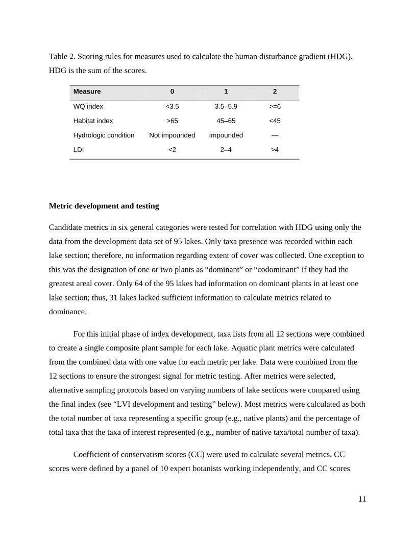
Table 2. Scoring rules for measures used to calculate the human disturbance gradient (HDG).

HDG is the sum of the scores.

Measure 0 1 2

WQ index <3.5 3.5–5.9 >=6

Habitat index >65 45–65 <45

Hydrologic condition Not impounded Impounded —

LDI <2 2–4 >4

Metric development and testing

Candidate metrics in six general categories were tested for correlation with HDG using only the

data from the development data set of 95 lakes. Only taxa presence was recorded within each

lake section; therefore, no information regarding extent of cover was collected. One exception to

this was the designation of one or two plants as “dominant” or “codominant” if they had the

greatest areal cover. Only 64 of the 95 lakes had information on dominant plants in at least one

lake section; thus, 31 lakes lacked sufficient information to calculate metrics related to

dominance.

For this initial phase of index development, taxa lists from all 12 sections were combined

to create a single composite plant sample for each lake. Aquatic plant metrics were calculated

from the combined data with one value for each metric per lake. Data were combined from the

12 sections to ensure the strongest signal for metric testing. After metrics were selected,

alternative sampling protocols based on varying numbers of lake sections were compared using

the final index (see “LVI development and testing” below). Most metrics were calculated as both

the total number of taxa representing a specific group (e.g., native plants) and the percentage of

total taxa that the taxa of interest represented (e.g., number of native taxa/total number of taxa).

Coefficient of conservatism scores (CC) were used to calculate several metrics. CC

scores were defined by a panel of 10 expert botanists working independently, and CC scores

12

from each expert were averaged to derive a single CC score for each taxon. The CC scores were

developed for depressional marshes in Florida, not for lakes (Cohen et al., 2004).

Community structure – The total number of taxa found is expected to decline as human

disturbance eliminates habitat, changes water chemistry, and interrupts the natural hydroperiod.

Although some studies have documented a decline in the number of wetland taxa as disturbance

increases (Findlay and Houlahan,1997; Lopez et al., 2002), this metric is not typically chosen for

wetland monitoring (USEPA, 2002c). The number of plant guilds summarized the number of

different types of plants present at a lake, e.g., forb/herb, graminoid, shrub, tree, or vine. The

number of plant guilds is expected to decline with disturbance. We expect more tolerant plants to

dominate the assemblage as disturbance increases. Dominant C of C was defined as the CC score

for the one or two plants that covered the greatest area.

Nativity – Native taxa are those whose natural range included Florida at the time of European

contact (1500 AD). Exotic taxa are species introduced to Florida from a natural range outside of

Florida. Definitions of invasive taxa were taken from lists developed by the Florida Exotic Pest

Plant Council (FLEPPC). FLEPPC defines Category I invasives as “exotics that are altering

native plant communities by displacing native species, changing community structures or

ecological functions, or hybridizing with natives” (FLEPPC, 2003). Category II invasives are

defined as “exotics that have increased in abundance or frequency but have not yet altered

Florida plant communities to the extent shown by Category I species.” For 95 lakes in the

development data set, 17 taxa were listed as Category I and 7 as Category II. (See Appendix 1

for plant attributes.)

Threatened and endangered species – Four endangered species (Xyris isoetifolia, Hypericum

lissophloeus, Salix eriocephala, and S. floridana) and one threatened species were found

(Drosera intermedia). Five species did not provide enough range of values to define a metric and

no metric was tested for this attribute.

Tolerance/Sensitivity – Coefficient of conservatism (CC) scores were available for 240 of the

404 taxa found. CC scores are most typically used to calculate a ‘floristic quality index (FQI)’

(Lopez and Fennessy, 2002). FQI was calculated as the average CC value multiplied by the

square root of the total number of plant taxa. The simple mean of the CC scores has also been

13

reported and was tested here. Lane et al. (2004) found that mean CC score was significantly

correlated with LDI for herbaceous wetlands in Florida. We calculated the total number of

sensitive and tolerant taxa by defining taxa with a CC score > 7 to be sensitive and CC < 3 to be

tolerant (Table 3). Percent sensitive and tolerant taxa were selected as metrics for both the

herbaceous and forested wetland indices in Florida (Lane et al., 2004; Reiss and Brown, 2005).

Duration – Lakes with less human disturbance are expected to have a greater number of

perennial taxa or a higher relative proportion of perennial taxa than annual taxa. Annual taxa

represent more opportunistic taxa which tend to be associated with human disturbance. Ohio

EPA uses the ratio of annual to perennial taxa in several of its vegetation indices for wetlands

(Mack, 2004).

Table 3. Coefficient of conservatism (CC) scoring criteria (after Cohen et at., 2004; Andreas 1995) and designations used to define a plant as tolerant or sensitive for this study.

CC score

Sensitive or Tolerant

Criteria

0 T Alien taxa and native taxa that are opportunistic invaders 1–3 T Widespread taxa that are found in a variety of communities,

including disturbed sites 4–6 Neither Taxa that display fidelity to a particular community, but tolerate

moderate disturbance 7–8 S Taxa that are typical of well-established communities, which have

sustained only minor disturbances 9–10 S Taxa that exhibit high degrees of fidelity to a narrow set of

ecological conditions

Wetland status – Although all sampling locations were defined as lakes and not wetlands, we

tested metrics related to wetland status because extensive lists have been developed for many

plants and because wetland status may provide an indicator of hydrologic alteration or other

types of human disturbance in lakes (USEPA, 2002c). Species defined as ‘obligate wetland’ or

‘facultative wetland’ plants are considered to be adapted to life in anaerobic soils (USACE,

1987); facultative species are equally likely to occur in wetlands or non-wetlands; and upland

species are expected not to occur in wetlands.

14

Growth form – This category included several aspects of plant growth. Metrics were calculated

for herbaceous and woody taxa and for emergent, floating, and submersed taxa. Fern and

gymnosperm taxa were also summarized. The previous metrics were also calculated for native

taxa only. In addition, candidate metrics based on native forbs+herbs, graminoids, nonvascular

plants, vines, shrubs, subshrubs and trees were tested. Nichols et al. (2000) suggest that the

relative frequency of submersed taxa may be greater than floating or emergent taxa when water

quality is degraded. Emergent species may also tolerate greater wave action. Other studies

suggest that emergent species may increase with an increase in nutrients, while submersed taxa

decline (Doherty et al., 2000).

Dicot/monocot – Flowering plants (angiosperms) are divided into two groups depending on the

number of cotyledons found in the embryo. The cotyledons are the seed leaves produced by the

embryo. In Ohio, native dicots decline with increasing disturbance, and this metric is included in

four out of five Ohio wetland indices (Mack, 2004).

Additional metrics derived from the national wetland database – In addition, several metrics

were derived from a national database of plant characteristics developed for wetland plants

(Adamus and Gonyaw, 2000). Information in this database was derived from published, peer-

reviewed studies. Development of this database was funded by EPA in response to requests from

state agencies involved in monitoring wetlands. The attributes were derived from literature

surveys for each taxon and summarized information regarding general sensitivity or tolerance,

tolerance to nutrients, nitrogen or phosphorus, and sensitivity or tolerance to flooding, sediment,

and salinity (Appendix 2). Of the 404 taxa found in the 95 lakes, 137 were listed in the EPA

database.

Sensitive and tolerant taxa evaluation

We tested the association of individual plant taxa with the HDG using a 2 x 2 contingency table

analysis (χ2, Yates correction, α = 0.05). Lakes with an HDG of 0, 1, or 2 were defined as ‘good’

lakes (N = 36), and the remaining 59 lakes with HDG from 3–7 as the ‘poor’ lakes. An HDG < 3

meant that a lake could have moderate disturbance indicated for two measures or high

disturbance for a single indicator. This statistical approach tests whether occurrence of an

individual plant taxon depended on the level of human disturbance.

15

We also calculated the average HDG value for all the lakes at which a particular taxon

was found and compared this empirical value for sensitivity (or tolerance) to the CC values

derived from expert judgment. This approach was not intended as a potential metric, but as a test

of the CC scores for the lakes data set.

Lake Vegetation Index (LVI) development and testing

Candidate metrics were considered for inclusion in the LVI if they were significantly correlated

with the HDG (Spearman’s r >= 0.4 or <= –0.4), the correlation was in the predicted direction,

and the metric was not redundant with another metric.

After selecting metrics to be included in the LVI, additional tasks remained before

finalizing the details of index calculation. First, we tested for correlation between LVI and lake

surface area, latitude and longitude. Second, we used data from the 12 lake sections to compare

alternative sampling protocols in order to determine the most efficient method for collecting

plant data from a lake. From that analysis we defined the final protocol for the LVI to be based

on the average of 4 replicate LVI values from 4 lake sections. Using this version of the LVI, we

tested that the patterns of correlation observed in the original 95 lakes were valid, using an

independent data set of 63 lakes to test for correlation between LVI and HDG. Finally, we

evaluated seasonal differences for 15 lakes with LVI sampling during both spring and summer.

There were numerous choices in how to calculate the LVI from the 12 taxa lists for each

lake visit. We used three versions of the LVI for different aspects of index testing and

development and denoted the different versions with suffixes. The three versions of LVI were

calculated as:

LVI_1x – one sample from each of 12 sections, N = 12 per lake-visit,

LVI_2x – one sample equals the combination of data from two sections from opposite sides of the lake, N = 6 per lake-visit, and

LVI_12x – one sample per lake derived from the combination of data from all 12 lake sections, N = 1 per lake-visit.

Additional versions of the index could be calculated, for example, by combining data from 3 or 4

lake sections. We did not pursue these other combinations because results for these three

16

versions were so similar. Furthermore, we were interested in the smallest amount of sampling in

order to minimize field effort.

For all three versions of the LVI, the index was calculated by first transforming metrics

into unit-less scores on the basis of their 5th and 95th percentiles. Leaving out the upper and lower

5% of metric values eliminates extremely high or low values that may not be typical of

minimally or extremely disturbed sites. The 95th percentile value was assigned a score of 10 (for

metrics that declined with disturbance such as percent native taxa) and the 5th percentile value

was assigned a score of 0. For metrics that increased with disturbance, the scores were reversed

for the 5th and 95th percentiles. After transformation, metric scores ranged from 0–10. The LVI

was the sum of the four metrics multiplied by a constant to adjust the range of LVI to a 0–100

scale. A scale from 0–100 was selected for convenience with the intention of keeping the same

scale for all Florida multimetric indices (Hughes et al., 1998).

We used non-parametric correlation to test association between LVI_12x and lake

surface area, latitude, and longitude. Because LVI_12X was significantly correlated with latitude

as well as HDG, we used multiple regression to evaluate the relationship between LVI_12x and

these independent variables. After confirming that human disturbance was the primary correlate

for both LVI_12x and its component metrics, we next addressed the question of how many lake

sections should be sampled. We evaluated the different versions of the index using two criteria:

1) LVI correlation with human disturbance and 2) the number of categories of biological

condition that each version of the index could detect.

We estimated within-lake variability of the different versions of LVI using an ANOVA

model. We used lake as the main factor and repeat samples within each lake were defined as

replicates and used to calculate the mean squared error (MSE). This estimate of variance was

used to calculate a 90% confidence interval for different versions of LVI (Zar, 1984). The

confidence interval was calculated as:

17

LVI ⎟⎟⎠

⎞⎜⎜⎝

⎛± 645.1*

2

ns

,

where s2 = variance estimated from ANOVA (mean squared error), and

n = number of samples taken from the lake.

The number of categories of biological condition that LVI can reliably detect was

obtained by dividing the possible range of the index (0–100) by the confidence interval. Thus,

the confidence interval defined the level of precision of the index by representing how different

LVI would have to be during a subsequent lake-visit to conclude that a statistically significant

change had occurred in lake condition. That confidence interval was also used to define how

many non-overlapping categories of biological condition could be defined over the potential

range of LVI. To compare the different versions of LVI, we looked at the number of categories

of biological condition each version could reliably detect for different numbers of replicate

samples.

We used z-values from the normal distribution to calculate 90% confidence limits for

LVI for two reasons. First, the distribution of multimetric indices are known to approximate the

normal distribution in that they are unimodal and symmetric (Fore et al., 1994). Second, for

small sample sizes, the t-distribution is appropriate for calculating confidence limits because

variance may be underestimated; however, for large sample sizes (df > 30) the two distributions

converge. For this data set, data from 95 lakes provided an adequate sample size to apply the

normal distribution. An additional concern when estimating variance is that the full range of

expected values are represented. LVI values for this data set ranged from 0–100, which included

all possible values for the index.

To validate the results based on the development data set of 95 lakes, an additional 63

lakes were sampled in 2004. LVI, HDG, the WQ index, the habitat index and LDI were

calculated for these additional lakes and tested for correlation. Fifteen of these lakes were

sampled twice during 2004, once during spring (March–April) and again during the summer

(July–August).

18

Expectations for statistical correlation

The statistical significance of a correlation coefficient (r) is a function of the sample size, such

that for larger sample sizes a smaller correlation coefficient will be significant. For large data

sets, e.g., N = 100, a correlation coefficient of 0.17 will be statistically significant (alpha = 0.05,

1-sided test). Such a small correlation coefficient may be statistically significant but biologically

not very meaningful. Consequently, before correlation testing is complete, a scientist should

consider the underlying meaning of correlation coefficients and what values represent biological

significance.

Based on these considerations, we selected specific values for correlation coefficients that

would represent a meaningful association depending on which relationship was being tested. We

used a correlation coefficient for metrics > 0.4 to define a significant relationship with HDG,

then further evaluated each metric by looking at scatter plots. Thus, for metric selection, a higher

standard was set than simple statistical significance. For metric correlation with the HDG, we

anticipated that the variability associated with HDG and the inherent difficulty involved in fully

assessing human influence would mean that high correlation coefficients (e.g., > 0.7) would be

unlikely. On the other hand, correlation coefficients < 0.4, though they may be statistically

significant, tend to be unconvincing when graphed.

Using graphs, we tested to be sure that the lack of correlation was not due to good metric

values in sites where human disturbance was known to be high. In contrast, we tolerated poor

metric values in sites with no known disturbance because the HDG does not include many

potential sources of degradation (e.g., herbicides).

To test for metric redundancy, we first screened metrics to determine whether a metric

pair’s correlation was greater than 0.8. We expected metrics to be highly correlated with each

other because they were initially selected for their correlation with the same underlying measure,

the HDG. When selecting metrics for the LVI, we wanted to be sure that the metrics were not

redundant in that they were derived from the same information (species). If a metric pair was

highly correlated, we evaluated the metrics to determine whether the same taxa were used in

calculation of both metrics. When metrics were derived from redundant information, one metric

19

in each pair (or group) was selected on the basis of its correlation with HDG, biological meaning,

and sensitivity to degradation.

When testing for correlation between biological measures (LVI and its component

metrics) and physical measures (lake surface area, latitude, and longitude), we were less tolerant

of correlation. For this analysis, any statistical significant correlation was considered because we

were concerned that underlying natural features or processes could bias the biological assessment

of LVI. We wanted to be sure that smaller lakes, for example, did not consistently score lower

for LVI for the same level of human disturbance. Thus, in different testing situations, different

values for the correlation coefficient were selected to indicate a significant association before

testing.

20

RESULTS

A total of 404 taxa were identified from the 95 lakes in the index development data set. Most

plants were identified to species, in some cases plants were identified to genus (e.g., Bidens,

Cyperus, Ludwigia, Panicum, Xyris), and in a very few cases to family. The number of taxa

identified in a lake based on the combination of data from all 12 sections ranged from 13–57,

with an average of 34 taxa. The number of taxa found in a single lake section (1 of 12) ranged

from 1–44 with an average of 15 taxa (Kell-Air and Karick Lakes had the lowest value of one

taxon in a section and Lake Juliana had 44 taxa in one section).

Human disturbance gradient

The HDG was highly correlated with its component measures, indicating that HDG effectively

integrated site condition for all three component measures (Table 4). Overall, each individual

measure of human disturbance was more highly correlated with the HDG than with other

measures, suggesting that the HDG was a better measure of general human disturbance.

Hydrologic condition was not tested for correlation because it had only two possible values. The

WQ and habitat indices were also highly correlated with each other, as were the habitat index

and the LDI. In contrast, the WQ index was not significantly correlated with LDI, indicating that

land use was not a good predictor of water quality condition for this data set. When only sites

with no missing values for water quality variables were tested for correlation, values for the

correlation coefficient changed little (< 0.04).

Table 4. Correlation for measures of human disturbance and the HDG, only significant correlations are shown (Spearman’s r, p < 0.01). Index values were tested for correlation using their original values, not the scores (0, 1, 2) used to calculate the HDG.

HDG WQ index Habitat index LDI

HDG 0.62 -0.87 0.73

WQ index 0.62 -0.46

Habitat index -0.87 -0.46 -0.69

LDI 0.73 -0.69

21

Because the WQ index and LDI were not highly correlated, we tested whether soil type

could explain the lack of correlation (Florida GIS coverage STATSGO soils). Some soils are

more porous than others and for lakes in porous soils, chemicals or pollutants may run into the

soil rather than run off the surface and into the lake. Lakes surrounded by non-porous soils may

have higher levels of chemicals. We used a nonparametric two-sample test to check for

differences in the WQ index, conductivity, NH3, TKN, NOx, TP, orthophosphates (OP), chloride,

and sulfate. Conductivity, TP, and TKN were significantly higher in lakes with non-porous soils

(Mann-Whitney U test, 1-sided, p < 0.05; Table 5). NOx was significant, but not in the direction

predicted, values were lower in lakes with non-porous soil. Though statistically significant, the

differences between levels of chemical measures in porous and non-porous soils were probably

not large enough to explain the lack of correlation between the WQ index and LDI.

Table 5. Water quality measure, and statistics from Mann-Whitney U test including rank sums for non-porous (NP) and porous (P) soils, U-statistic, z-statistic, sample size (N), and p-value. Significantly different measures are marked with an *.

WQ measure Rank Sum NP Rank Sum P U Z N (NP) N (P) p

WQ index 1901.0 2285.0 959.0 0.49 40 51 0.31

* Conductivity 2070.5 2024.5 749.5 2.03 40 50 0.02

* TKN 1662.0 1824.0 648.0 1.77 35 48 0.04

NOX 1294.0 2361.0 591.0 -2.63 37 48 0.00

* TP 1972.5 1855.5 630.5 2.57 38 49 0.01

AGP 1273.5 1576.5 678.5 -0.20 34 41 0.42

OP 564.0 517.0 264.0 0.00 24 22 0.50

NH3_N 1624.5 2203.5 883.5 -0.41 38 49 0.34

Chloride 371.0 532.0 181.0 0.70 16 26 0.24

Sulfate 390.0 513.0 162.0 1.19 16 26 0.12

Metric selection

Many candidate metrics were tested and relatively few were strongly correlated with HDG or

consistently correlated with the other measures of human disturbance. Of the 65 metrics tested

for correlation with HDG, only 10 had an r-value > 0.4 (or < –0.4; Table 6). Because many of

these metrics were redundant, a total of four metrics were selected for the final multimetric

index. In general, if a candidate metric was correlated with HDG when calculated as number of

22

taxa, it was also correlated with HDG when calculated as percentage of total taxa. In addition, if

a candidate metric was correlated with HDG, it was typically correlated with at least two of the

other measures of disturbance.

Overall, the metrics that measured the numbers of native and exotic taxa and metrics

derived from CC values were the most consistently associated with human disturbance. Within

specific metric categories, results for individual metrics tended to be similar. Of the three metrics

related to community structure, only dominant C of C (defined as the CC score for the one or

two plants that covered the greatest area) was significantly correlated with HDG and was

included in the index. A total of 63 taxa were identified as dominant in at least one lake section.

Of these 63 taxa, about 1/3 were identified only once and about 1/3 were identified >10 times as

dominant (Table 7). Total number of taxa and the total number of growth forms were not

correlated with HDG.

Of the four metrics related to nativity, all were significantly correlated with HDG, but the

three based on exotic taxa were redundant. Category I and II invasives represented a subset of

the exotic taxa. We retained percent invasive taxa for the LVI because invasive taxa represent a

significant economic concern and an objective threat to native plant assemblages. We calculated

this metric as a percentage of total taxa rather than total number of taxa because this form of the

metric was less affected by geographic factors such as latitude. We also included percent native

taxa in the index, which was only significantly associated with HDG when calculated as a

percentage of total taxa.

23

Table 6. Candidate plant metrics and their correlation with HDG, the WQ index, LDI, and the habitat index. Only Spearman’s correlations >0.40 are shown ( p < 0.001). The sample size is shown for all metrics except dominant C of C for which N ranged from 57–65. Most metrics were calculated as both the total number of taxa and the percentage of total taxa (left vs. right side of table); exceptions to this were metrics in the category “Community structure” which could only be calculated in one way. The source of information for each metric is listed. Similar metrics calculated from the national EPA database are also shown (Adamus and Gonyaw, 2000). Metrics selected for the final index are marked (“*”).

Number of taxa Percent of total taxa HDG WQ LDI Habitat HDG WQ LDI Habitat Source

N = 95 95 93 90 95 95 93 90 Community structure Total taxa – – – – FDEP No. of plant guilds – – – – FDEP * Dominant C of C -0.52 -0.43 0.49 – – – – FDEP Nativity * Native -0.56 -0.46 -0.53 0.64 FDEP Exotic 0.55 0.50 0.45 -0.48 0.63 0.51 0.61 -0.65 FDEP Category 1 0.56 0.44 0.48 -0.50 0.58 0.43 0.58 -0.58 FLEPPC * Categories 1 & 2 0.59 0.51 0.49 -0.53 0.62 0.48 0.60 -0.62 FLEPPC Tolerance FQI Score -0.52 -0.32 -0.54 0.57 – – – – FDEP Average CC -0.67 -0.49 -0.59 0.63 – – – – CC * Sensitive (CC > 7) -0.40 -0.41 0.46 -0.49 -0.44 -0.41 0.48 CC Tolerant (CC < 3) 0.48 0.67 0.42 0.60 -0.59 CC V. Tolerant (CC < 2) 0.51 0.40 -0.40 0.65 0.41 0.59 -0.59 CC Duration Perennial FDEP Annual FDEP Annual:Perennial ratio FDEP Native A:P ratio FDEP Native perennials FDEP Native annuals FDEP Wetland status Obligate wetland FDEP Obligate + facultative FDEP Upland FDEP Native obligate wetland FDEP Native facult. wetland FDEP Native upland FDEP Growth form Herbaceous FDEP Woody FDEP Emergent FDEP Floating FDEP Submersed FDEP Fern FDEP Gymnosperm FDEP

24

Number of taxa Percent of total taxa HDG WQ LDI Habitat HDG WQ LDI Habitat Source

N = 95 95 93 90 95 95 93 90 Native herbaceous FDEP Native woody -0.48 FDEP Native emergent FDEP Native floating FDEP Native submersed FDEP Native fern FDEP Native gymnosperm FDEP Native forbs + herbs FDEP Native graminoids FDEP Native vines FDEP Native shrubs -0.44 -0.52 0.48 -0.41 FDEP Native subshrubs FDEP Native tree FDEP Dicot/monocot Dicot FDEP Monocot FDEP Native dicot -0.40 FDEP Native monocot FDEP EPA database Sensitive EPA Tolerant EPA V. Tolerant EPA Nutrient tolerant EPA V. Nutrient tolerant EPA N tolerant EPA P sensitive EPA P tolerant -0.41 EPA Flood sensitive -0.40 EPA Flood tolerant -0.43 EPA V. Flood tolerant EPA Sediment sensitive 0.40 EPA Sediment tolerant -0.40 0.43 -0.41 -0.40 0.41 EPA V. Sediment tolerant EPA Salinity sensitive EPA Salinity tolerant EPA V. salinity tolerant EPA

25

Table 7. List of plant taxa that were most frequently identified as the dominant (or co-dominant) taxon in a lake section. Shown are the number of times the taxon was named dominant (or co-dominant) out of 786 occasions when dominant taxa were noted and CC score for that taxon.

Taxon Number of times CC scorePanicum repens 169 0Panicum hemitomon 164 5.82Typha domingensis 37 0.59Nuphar luteum 32 4.64Typha latifolia 32 1.6Mayaca fluviatilis 27 8.45Hydrilla verticillata 26 0Panicum 20 Taxodium ascendens 19 7.21Ludwigia octovalvis 17 4.09Nymphaea odorata 17 7.18Vallisneria americana 17 7.28Eichhornia crassipes 16 0Cladium jamaicense 12 9.04Fuirena scirpoidea 12 6.5Hypericum fasciculatum 12 7.27Hypericum lissophloeus 11

Of the five metrics related to tolerance and sensitivity, all were significantly correlated

with HDG. FQI score and average CC represented a general measure of overall tolerance, while

the number (or percentage) of tolerant or sensitive taxa represented opposite ends of the

spectrum. The general metrics that summarized sensitivity (or tolerance) of the entire plant

assemblage were redundant with the more specific metrics that measured either tolerance or

sensitivity. Of these, we selected the more specific metric, percentage sensitive taxa, for

inclusion in the index. Other studies have found that metrics related to sensitive or intolerant taxa

are the first to register changes in an assemblage when human disturbance is introduced into new

locations (Karr and Chu, 1999). We did not include percent tolerant taxa in the index because

many of the same plant taxa were also included in the invasive or exotic metrics.

Other candidate metrics related to duration of life cycle, wetland status, and number of

cotyledons were not correlated with HDG. Similarly, candidate metrics based on growth form or

26

type were not correlated with HDG, with the exception of one metric, number of native shrub

taxa, which was significantly correlated with HDG, LDI and the habitat index. This metric was

not included in the final index for two reasons. First, very few shrub taxa are typically found at a

lake and, second, of these few, some are indicators of disturbed conditions (e.g., Baccharis and

Sambucus).

The candidate metrics derived from the EPA database failed to correlate predictably or

consistently with HDG or other measures of disturbance. The sediment sensitive and sediment

tolerant metrics were significantly correlated with HDG but in the opposite direction predicted,

and so were not retained for the index.

Of the metrics correlated with HDG, r-values were generally higher when calculated as

percentage of total taxa rather than as number of taxa, probably because the total number of taxa

varied as a function of other natural features and calculation based on a percentage of total taxa

controlled for that source of variability.

The four metrics included in the LVI were all significantly correlated with each other, as

expected, but correlation coefficients were not high enough to warrant concerns regarding

redundancy of metrics. Correlation coefficients were < 0.8 (or > -0.8) for all metrics. More

importantly, the metrics were based on different sets of taxa with minimal overlap.

The four metrics selected for inclusion in the LVI, percent native taxa, percent invasive

taxa, percent sensitive taxa and dominant C of C, were correlated with HDG and its component

measures (Figures 3–6). Both percent invasive taxa and dominant C of C showed regional

differences in the panhandle and peninsula, and metric scores were adjusted for percent invasive

taxa by calculating the 5th and 95th percentiles separately for each region. Metric scoring for

dominant C of C was not adjusted for region, but should be reconsidered as more data become

available. Dominant C of C had three lakes with values that were outliers, that is, dominant C of

C was high in three lakes that also had high values for HDG. For these lakes, dominant plants

with high CC scores were Panicum hemitomon (CC = 5.82) and Vallisneria americana (CC =

7.28).

27

HDG

% N

ativ

e ta

xa

-1 0 1 2 3 4 5 6 7 810%

30%

50%

70%

90%

HDG

% In

vasi

ve ta

xa

-1 0 1 2 3 4 5 6 7 8

0%

20%

40%

60%

HDG

% S

ensi

tive

taxa

-1 0 1 2 3 4 5 6 7 8

0%

20%

40%

60%

HDG

Dom

inan

t C o

f C

-1 0 1 2 3 4 5 6 7 80

2

4

6

8

PeninsulaPanhandle

Figure 3. Metrics selected as components of LVI were strongly correlated with the human disturbance gradient (HDG). Percent invasive taxa and dominant C of C differed slightly in the peninsula and panhandle for the same values of HDG. Each point represents a single lake; lines are least fit regression lines for each geographic area. Four lakes from the NE region are not shown.

28

1 2 3 4 5 6 7 8 9 10WQ index

10%

30%

50%

70%

90%%

Nat

ive

taxa

1 2 3 4 5 6 7 8 9 10WQ index

0%

20%

40%

60%

% In

vasi

ve ta

xa

1 2 3 4 5 6 7 8 9 10WQ index

0%10%20%30%40%50%60%

% S

ensi

tive

taxa

1 2 3 4 5 6 7 8 9 10WQ index

-1012345678

Dom

inan

t C o

f C

Figure 4. LVI metrics were highly correlated with the water quality index. Each point represents a single lake.

29

0 20 40 60 80 100Habitat index

10%

30%

50%

70%

90%

% N

ativ

e ta

xa

0 20 40 60 80 100Habitat index

0%

20%

40%

60%

% In

vasi

ve ta

xa

0 20 40 60 80 100Habitat index

0%

20%

40%

60%

% S

ensi

tive

taxa

0 20 40 60 80 100Habitat index

0

2

4

6

8

Dom

inan

t C o

f C

Figure 5. LVI metrics were highly correlated with the habitat index. Each point represents a single lake.

30

0 1 2 3 4 5 6 7 8 9LDI

10%

30%

50%

70%

90%

% N

ativ

e ta

xa

0 1 2 3 4 5 6 7 8 9LDI

0%

20%

40%

60%

% In

vasi

ve ta

xa

0 1 2 3 4 5 6 7 8 9LDI

0%

20%

40%

60%

% S

ensi

tive

taxa

0 1 2 3 4 5 6 7 8LDI

0

2

4

6

8

Dom

inan

t C o

f C

Figure 6. LVI metrics were highly correlated with the LDI index. Each point represents a single lake.

31

Sensitive and tolerant taxa

Of the 404 taxa found in 95 lakes, 62 were defined as sensitive (CC score > 7) and 47 as tolerant

(CC < 3) based on professional judgment (Cohen et al., 2004). Not all these assignments could

be tested using the data from 95 lakes because so many taxa were rare. More than half of the taxa

occurred in < 5 lakes (248 out of 404, or 61%). Of the 62 taxa defined as sensitive, 35 (56%)

occurred in < 5 lakes; of the 47 tolerant taxa, 19 (40%) occurred in < 5 lakes. These taxa

occurred in too few lakes to be tested for their association with HDG.

Of the taxa that occurred frequently enough to test, relatively few (29 of 404, or 7%)

showed an association with HDG that was statistically significant (χ2, p < 0.05). Nine sensitive

taxa and 11 tolerant taxa were significantly associated with disturbance (Table 8; see Appendix 3

for all taxa). One species, Vallisneria americana, was defined as sensitive on the basis of its CC

score, but was significantly associated with more disturbed lakes for this data set indicating that

this taxon may be incorrectly defined for lakes. In general, most of the other taxa that showed a

statistically significant association with HDG agreed with their CC scores in terms of their

preference for undisturbed or disturbed conditions.

Although statistically significant, the preferences for ‘good’ or ‘poor’ lakes were not

strong in several cases. For example, Cephalanthus occidentalis showed a significant preference

with 25 out of 51 occurrences in ‘good’ sites although the preference represented only 49% of its

occurrences. From a statistical point of view, the association may be better than chance (which

was equal to 38% of occurrences at good sites); however, from a biological point of view, 51%

of its occurrences in ‘poor’ sites does not indicate a sensitive species. For this reason, a similar

analysis of macroinvertebrates in streams set the criteria for defining sensitive taxa much higher

(87% of occurrences in good sites) than statistical significance (Fore, 2004).

We continued to use the sensitive and tolerant taxa lists derived from the panel of expert

botanists rather than define a list based on the results of this statistical analysis for two reasons.

First, most of the taxa were too rare to test with these data. In addition, the statistical analysis for

these data yielded too few taxa to define reliable metrics for sensitive or tolerant taxa.

32

Table 8. Taxa that were significantly associated with low or high HDG (χ2, p < 0.05). Shown are taxon name, CC value, whether the taxon was identified as sensitive or tolerant based on CC value, number of lakes in which taxon was found out of 95 lakes, number of occurrences in ‘good’ lakes (HDG < 3) and ‘bad’ lakes (HDG >= 3), proportion of total occurrences in good lakes, and whether the direction of taxon preference agreed with the CC value.

Taxon CC Sens/Tol # Occur # Good # Bad %Good Agree

Vallisneria americana 7.28 S 18 2 16 0.11 no Cephalanthus occidentalis 7.27 S 51 25 26 0.49 yes Cladium jamaicense 9.04 S 22 15 7 0.68 yes Decodon verticillatus 7.8 S 12 10 2 0.83 yes Hypericum fasciculatum 7.27 S 13 10 3 0.77 yes Lyonia lucida 7.06 S 8 7 1 0.88 yes Mayaca fluviatilis 8.45 S 19 12 7 0.63 yes Nymphaea odorata 7.18 S 43 22 21 0.51 yes Triadenum virginicum 8.16 S 17 11 6 0.65 yes Alternanthera philoxeroides 0 T 49 10 39 0.20 yes Brachiaria mutica 0 T 18 2 16 0.11 yes Colocasia esculenta 0 T 40 7 33 0.18 yes Cyperus surinamensis 2.03 T 14 1 13 0.07 yes Hydrilla verticillata 0 T 19 1 18 0.05 yes Ludwigia peruviana 0.62 T 42 10 32 0.24 yes Mikania scandens 1.95 T 65 16 49 0.25 yes Panicum repens 0 T 73 23 50 0.32 yes Pistia stratiotes 0 T 15 1 14 0.07 yes Sapium sebiferum 0 T 21 3 18 0.14 yes Schinus terebinthifolius 0 T 34 6 28 0.18 yes Ludwigia alata 5.85 4 4 0 1.00 unk Nymphoides aquatica 6.09 17 13 4 0.76 unk Utricularia purpurea 6.5 7 6 1 0.86 unk Cabomba caroliniana 5.07 9 7 2 0.78 unk Cyperus odoratus 4.25 27 3 24 0.11 unk Lachnanthes caroliana 3.76 24 16 8 0.67 unk Scirpus cyperinus na 4 4 0 1.00 unk Solidago na 17 12 5 0.71 unk Utricularia na 18 11 7 0.61 unk

33

1 2 3 4 5 6 7Taxon average HDG

0

2

4

6

8

10

Taxo

n C

C

Figure 7. Plant CC value declined as the average HDG for the lakes at which a taxon was found increased (Spearman’s r = -0.42, r2 = 0.18, p < 0.01, N = 123 taxa). Shown are results for taxa with >4 occurrences in 95 lakes.

Cohen et al. (2004) describe another approach for comparing field data with CC scores.

For each taxon, they calculated the average LDI value for all the sites at which the taxon was

found. We followed their approach using HDG instead of LDI. We averaged the HDG values for

each lake in which a particular taxon was found. We compared the average HDG values for each

taxon with the CC score for each taxon and found that they were significantly correlated

(Spearman’s r = –0.42, N = 123 taxa, p < 0.01). Although statistically significant, the agreement

between the CC values based on expert opinion and the average HDG value at all sites in which

a taxon was found was not close (r2 = 0.18; Figure 7).

Evaluation of the Lake Vegetation Index (LVI)

The following sections describe results for 1) correlation analysis of LVI with human

disturbance and other natural geographic features; 2) selection of the most efficient lake

sampling protocol; 3) validation of LVI using an independent data set; 4) description of lakes

with higher or lower LVI values than predicted by the HDG (outliers); and 5) a comparison of

34

LVI values for lakes sampled during spring and summer. We compared different versions of LVI

using different numbers of lake sections and selected a final protocol based on LVI calculated

from 4 lake sections from opposite sides of the lake.

Correlation of LVI with human disturbance and natural features

For this initial testing of LVI, plant data from all lake sections were combined to obtain a single

LVI for each lake (LVI_12x). We anticipated that correlations with natural features might be

subtle and our goal was to use the most accurate LVI for this testing. (Subsequent analyses based

on smaller numbers of lake sections revealed index values differed little according to the number

of sections used in calculations.) LVI_12x was highly correlated with HDG and was more highly

correlated with HDG than other measures of human disturbance indicating the value of the HDG

as an integrated measure of disparate types of human disturbance (Table 9; Appendix 4).

LVI_12x was not correlated with lake size (surface area), which meant that adjustments to metric

scoring based on lake size were not necessary. LVI_12x was not significantly correlated with

longitude, but was correlated with latitude, probably because the HDG was also correlated with

latitude.

Table 9. Correlation coefficients for LVI_12x and measures of human disturbance, lake area, latitude and longitude. Non-significant correlations indicated by parentheses (Spearman’s r, p < 0.01).

HDG WQ index Habitat index LDI Area Latitude Longitude

N = 95 87 90 93 76 95 95

LVI_12x -0.68 -0.46 0.69 -0.62 (0.03) 0.35 (0.06)

The significant correlation between LVI_12x and latitude triggered a more detailed

analysis between these variables to ensure that human disturbance was the primary cause of

changes in LVI values and not spurious correlation with other natural features. We used multiple

regression to test for significant associations between LVI_12x and HDG, lake surface area, and

latitude (the independent variables) simultaneously. We also tested each of LVI’s component

metrics separately for association with the same independent measures to identify any

confounding relationships among the metrics.

35

LVI_12x was significantly correlated with HDG but not with area or latitude when all

three were included in a multiple regression model. Of the four metrics, only percent invasive

taxa was significantly associated with both latitude and HDG; the other three were only

significantly associated with HDG (Table 10). Adjustments to the metric scoring for panhandle

and peninsula areas helped to resolve the underlying correlation with geographic location for the

final LVI.

Multiple regression assumes that the independent variables (area, latitude, and longitude)

are independent and not correlated. For this analysis, HDG and latitude were significantly

correlated (Pearson’s r = 0.3, p < 0.01). Correlation among independent variables in a multiple

regression model can result in unstable solutions or inconsistent results. Correlation among

independent variables is difficult to avoid in regional surveys such as these because human land

use typically follows geographic gradients. Nonetheless, the consistent high correlation between

LVI_12x and its component metrics with HDG and consistent exclusion of latitude and area

from the model solution supports the conclusion that HDG was the primary source of variance in

LVI.

Table 10. Standardized regression coefficients from multiple regression. Each row represents a different statistical test for each biological measure. Column variables were entered in each model and only coefficients for significant predictors are shown. Only 76 lakes had information for lake surface area.

Biological measure

N HDG Latitude Area

LVI_12x 76 -0.68

% Native taxa 76 -0.50

% Invasive taxa 76 0.49 -0.28

% Sensitive taxa 76 -0.50

Dominant C of C 50 -0.62

Variability analysis of alternative lake sampling protocols

As expected, the total number of species increased as the number of lake sections increased from

1–12 (Figure 8). The percentage of the total taxa collected increased steadily, but an obvious

asymptote was not achieved. About half the taxa found in all 12 sections were found within a

36

single section when results were averaged across all 100 lake-visits (95 lakes with 5 lakes visited

twice; Table 11). For eight sections, 92% of the taxa (on average) were found. Results from this

analysis of species accumulation failed to identify an obvious asymptote for a particular number

of sections that could be used to define the minimum sampling effort for lake assessment and

LVI calculation. Therefore, we looked at the variability of LVI derived from different sampling

protocols to define how many lake sections should be sampled during each visit.

Table 11. The cumulative number of sections sampled per lake-visit, the proportion of the total taxa found for a given number of sections (averaged across all lake-visits), and the number of lake-visits that attained the maximum number of taxa found in all 12 sections for each number of sections sampled.

Number of sections 1 2 3 4 5 6 7 8 9 10 11 12

Mean of prop. of taxa 0.49 0.62 0.70 0.76 0.81 0.86 0.89 0.92 0.95 0.96 0.98 1.00

Number achieve max 0 0 0 2 5 6 9 13 21 41 62 100

1 2 3 4 5 6 7 8 9 10 11 12

Number of samples

20%

40%

60%

80%

100%

Per

cent

of s

peci

es a

ccum

ulat

ed

Mean Min-Max

Figure 8. Number of species increased as the number of lake sections sampled increased from 1–12. Averaged across all lakes, 49% of the taxa found in all 12 sections were found in one section. For two sections, 62% of the total taxa were collected.

37

Variance estimates for LVI were derived from ANOVA with lake as the main factor and

replicate samples in a lake used to calculate the within-lake variability (mean squared error). We

calculated variance for two versions of the LVI: 1) treating each of the 12 lake sections as

individual replicates (LVI_1x), and 2) combining data from two lake sections on opposite sides

of the lake, which yielded a total of 6 replicates per lake (LVI_2x). Within lake variance for

LVI_1x was ~50% greater than variance calculated for LVI_2x (Table 12). We used the variance

estimates for both versions of LVI to calculate confidence intervals. We divided the possible

range of the LVI (0–100) by the confidence interval to obtain the number of categories of

biological condition that each version of the index could detect.

If data were collected from a single lake section and LVI_1x calculated, 2.9 categories of

biological condition could be detected. If two replicate samples of this type were collected, 4.1

categories could be detected. For LVI_2x, if a single sample were collected (representing a

composite of data from two lake sections), 3.6 categories could be detected; if two samples of

this type were collected, 5.1 categories of condition could be detected. The two different

sampling approaches yielded similar levels of precision for an equivalent number of lake

sections (Figure 9). Two composite samples equals four single samples in terms of field effort,

and the two field methods yielded a similar number of categories: 5.7 vs. 5.1 (for LVI_1x vs.

LVI_2x).

Table 12. Two versions of the LVI, their variance estimates (MSE) for within lake sampling, and the number of categories of biological condition that could be detected for 1–6 replicate samples. Results are shown for two versions of the LVI calculated for 1) single section samples (LVI_1x) and 2) composite samples derived from two lake sections (LVI_2x).

Index version Variance Number of replicate samples

1 2 3 4 5 6

LVI_1x 112.33 2.87 4.06 4.97 5.74 6.41 7.02

LVI_2x 70.20 3.63 5.14 6.29 7.27 8.12 8.90

38

Num

ber o

f rep

licat

e sa

mpl

es

0 1 2 3 4 5 6 7 8 9 10

1

2

3

4

5

6

LVI_1x LVI_2x

Figure 9. The number of categories of biological condition that can be reliably detected increased as the number of replicate samples within each lake increased from 1 to 6. Shown are results for two versions of the LVI based on samples from a single section (LVI_1x) and composite samples composed of two lake sections (LVI_2x).

In addition to evaluating the statistical precision, we also tested whether LVI derived

from more lake sections was more highly correlated with HDG. In fact, correlation coefficients

were very similar for the three versions of LVI and for its component metrics (Table 13). Thus,

correlation with HDG did not improve with larger sample sizes (i.e., greater field effort), even

though the single sections had only half as many taxa as the composite samples based on data

from 12 lake sections. These results demonstrate that an exhaustive sample of all the plants in the

lake is not needed and that a consistent sample of a small subset of the plants present will

provide a reliable assessment of the plant assemblage. Based on these results, we selected the

LVI_1x version of the index for lake assessment. LVI_1x had a unimodal and fairly symmetric

distribution for the lakes in this data set (Figure 10).

39

Table 13. Correlation with HDG for LVI and its component metrics for three different sampling methods (Spearman’s r, p < 0.01).

Sampling method

LVI % Native taxa % Invasive taxa % Sensitive taxa Dominant C of C

N = 95 95 95 95 62 1x -0.70 -0.62 0.60 -0.49 -0.48

2x -0.70 -0.59 0.61 -0.48 -0.48

12x -0.68 -0.56 0.62 -0.49 -0.48

-10 10 30 50 70 90 110LVI_1x

0

40

80

120

160

200

Num

ber o

f obs

erva

tions

Figure 10. Distribution of LVI_1x for 12 replicate samples from 95 lakes. Curved line represents the normal distribution.

We used replicate samples of LVI_1x to test whether index values were more variable in

larger lakes than smaller lakes and found that they were not. In contrast, within-lake variance of

LVI_1x was higher in lakes with more human disturbance as measured by HDG (Spearman’s r =

0.38).

We also tested whether replicate sampling improved the accuracy of the lake assessment

for LVI_1x by averaging different numbers of lake replicates and correlating the average index

values with measures of human disturbance. The greatest improvement in correlation occurred

40

for one vs. two lake sections; improvements were incrementally smaller as more lake sections

were added to calculate the average LVI (Table 14). These results indicate that four replicate

samples of LVI_1x were sufficient to reliably assess a lake.

Table 14. Correlation between LVI_1x and measures of disturbance for different numbers of replicate samples within each lake (Spearman’s r, N = 95, p < 0.01).

Number of reps HDG WQ index Habitat index LDI

1 -0.60 -0.45 0.65 -0.40

2 -0.65 -0.46 0.70 -0.49

3 -0.66 -0.44 0.70 -0.53

4 -0.67 -0.46 0.69 -0.54

5 -0.66 -0.46 0.69 -0.54

6 -0.66 -0.48 0.68 -0.54

7 -0.67 -0.48 0.68 -0.55

8 -0.68 -0.49 0.68 -0.57

9 -0.69 -0.49 0.68 -0.58

10 -0.69 -0.50 0.68 -0.58

11 -0.70 -0.50 0.69 -0.59

12 -0.69 -0.51 0.68 -0.58

Metric scoring for the LVI

Percent invasive taxa differed slightly in metric values for similar values of HDG in the

peninsula and panhandle regions of the state. Metric scores were adjusted to ensure that an

equivalent level of human disturbance would translate into a similar LVI value independent of

location in the state (Table 15; see also Appendix 6). Several lakes had no information available

to calculate dominant C of C. For those lakes, we used the average of three (rather than four)

metric scores to calculate LVI.

41

Table 15. Metric scoring rules derived from the 5th and 95th percentiles. For percentage of taxa metrics, N = 1196 (12 sections in 100 lake-visits – 4 missing sections), but for Dominant C of C, N = 551. For dominant C of C, lakes in the northeast were scored as panhandle lakes. (See Appendix 6 for more recent scoring rules.)

Metric 5th %tile 95th %tile Scoring rule

% Native taxa 43% 95% (x – 43)/52

% Invasive taxa 0% 39%

Panhandle 0% 27% 1 – (x/27)

Peninsula 0% 40% 1 – (x/40)

% Sensitive taxa 0% 41% x/41

Dominant C of C 0 7.8 x/7.8

Validation of the LVI with independent data

LVI_1x calculated for the 63 independent lakes in the validation data set was highly correlated

with HDG (Table 16). Lakes in this data set provided a good test of the LVI because the lakes

represented a broad range of site conditions and included all possible values of HDG from 0–7

(Figure 11). LVI was also highly correlated with the habitat index and LDI; correlation was not

as high with the WQ index. These results were similar to those observed for the development

data set (see Table 9 above; see App. 6 for more recent validation).

The distribution of LVI values vs. HDG does not clearly illustrate the 5 non-overlapping

categories of biological condition that the variance analysis predicted. The 5 categories of

biological condition represent detectable levels of change for an individual lake. Figure 11 plots

LVI values from different lakes with similar values for HDG. In other words, the figure

introduces additional sources of variability for LVI associated with the type of disturbance or the

intensity of disturbance at a particular lake. Because the “true” value of human disturbance

cannot be accurately measured, lakes with approximately the same level of disturbance are

combined for similar values of HDG.

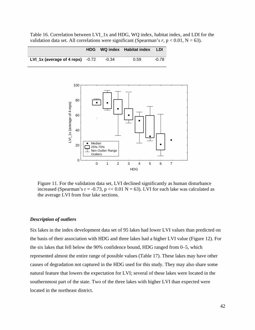
42

Table 16. Correlation between LVI_1x and HDG, WQ index, habitat index, and LDI for the validation data set. All correlations were significant (Spearman’s r, p < 0.01, N = 63).

HDG WQ index Habitat index LDI

LVI_1x (average of 4 reps) -0.72 -0.34 0.59 -0.78

0 1 2 3 4 5 6 7HDG

0

20

40

60

80

100

LVI_

1x (a

vera

ge o

f 4 re

ps)

Median 25%-75% Non-Outlier Range Outliers

Figure 11. For the validation data set, LVI declined significantly as human disturbance increased (Spearman’s r = -0.73, p << 0.01 N = 63). LVI for each lake was calculated as the average LVI from four lake sections.

Description of outliers

Six lakes in the index development data set of 95 lakes had lower LVI values than predicted on

the basis of their association with HDG and three lakes had a higher LVI value (Figure 12). For

the six lakes that fell below the 90% confidence bound, HDG ranged from 0–5, which

represented almost the entire range of possible values (Table 17). These lakes may have other

causes of degradation not captured in the HDG used for this study. They may also share some

natural feature that lowers the expectation for LVI; several of these lakes were located in the

southernmost part of the state. Two of the three lakes with higher LVI than expected were

located in the northeast district.

43

0 1 2 3 4 5 6 7 8HDG

0

20

40

60

80

100

IND

X_1

x

Figure 12. LVI declined as human disturbance increased. The regression line (solid) and the 90% confidence bounds (dotted) are shown, each point represents one lake (N = 95 lakes). Six lakes had lower LVI values than predicted by the HDG (open circles) and three lakes had an LVI slightly higher than predicted (open triangles).

Table 17. Lakes with higher or lower LVI values than expected based on HDG. Shown are the nickname, STORET, observed difference from expectation, region, district, LVI, HDG, WQ index, LDI and habitat index for each lake.

Nickname STORET Diff Region District LVI HDG WQ index

Hab index

LDI

L84-BANANA 27584418154127 Lower Peninsula SW 18.7 4 8.6 50.7 3.3LKLECLARE 28063598232193 Lower Peninsula SW 29.3 2 3.0 67.1 5.1L51PEAST 24040806 Lower Peninsula SW 26.8 3 5.0 6.2FRANTST 21020056 Higher Panhandle

East NE 69.4 5 5.2 12.9 7.2

LKHALPATOK 28010594 Lower Peninsula SE 47.9 0 2.4 66.4 1.4LAKEIDA 28010500 Lower Everglades SE 9.6 5 5.6 35.0 6.6LITTLE REF 26010636 Higher Peninsula S 87.8 2 89.3 TANKLAKE 20030151 Higher Peninsula NE 96.8 1 4.2 82.9 1.1L52PWALDEN 24040170 Lower Peninsula SW 9.1 3 6.0 3.1

44

Comparison of spring and summer LVI values

Some lakes had different LVI values in spring vs. summer, but higher LVI values were not

consistently associated with one season. LVI for five lakes were higher in spring, five lakes were

higher in summer, and five lakes were similar during both seasons (Figure 13). Because LVI was

higher in some lakes in spring and lower in others, no consistent seasonal association could be

identified and corrected. We could not discern from these data why some lakes were higher in

spring and others lower.

The observed differences may have occurred because some plants are easier to identify in

the spring due to the presence of flowers or seeds. Looking at the complete list of taxa for all 15

lakes, the number of individual plants that were not identified beyond genus was 8% during the

spring vs. 11% during the summer, a relatively small difference. Data from such a small data set

may be difficult to interpret; for example, 5 of the 15 sites had no invasive taxa recorded for

either season.

45

SR

1-SL

2004

SR

1-SL

2025

SR

1-SL

2028

SR

1-SL

2039

SR

1-SL

2059

SR

1-SL

2082

SR

1-SL

2087

SR

1-SL

2090

SR

1-SL

2094

SR

1-SL

2111

SR

1-SL

2117

SR

1-SL

2136

SR

1-SL

2153

SR

1-SL

2156

SR

1-SL

2171

10

30

50

70

90

LVI_

1x

Spring Summer

Figure 13. LVI for repeat visits to 15 lakes during the spring (closed circles) and summer (open triangles) of 2004. Each point represents the average LVI from four lake sections. Each lake-visit had three replicate samples of four sections each (4 x 3 = 12 lake sections).

46

DISCUSSION

When selecting biological measures as indicators of water body condition, two criteria must be

considered. First, the indicator must show a consistent and meaningful association with an

independent measure of human disturbance (Karr and Chu, 1999). Second, the indicator must be

sufficiently precise to detect changes in site condition should a change occur in order to be

protective of the resource (Fore, 2003). Metric selection for the LVI was relatively

straightforward because so few candidate metrics were reliably correlated with HDG. Those

metrics were also highly correlated with the other independent measures of disturbance. The LVI

was also precise enough to reliably detect five categories of biological condition based on

sampling 4 of 12 possible lake sections.

The LVI was highly correlated with HDG, more so than its component metrics, which

illustrates one of the advantages of a multimetric index: the index provides a more integrative

assessment of biological condition than a single metric. For multimetric indices, precision

typically increases with more metrics, and 7–10 metrics are preferred. Nonetheless, the precision

for LVI was quite high with only four metrics. LVI derived from four replicate lake sections had

sufficient statistical precision to reliably detect five categories of biological condition. Thus, the

LVI was both highly correlated with an independent measure of human disturbance and was very

precise for detecting changes in lake condition.

Human disturbance gradient

Human activities influence and degrade aquatic systems in multiple ways including the addition

of chemicals and nutrients to the water, destruction and loss of habitat, alteration of natural flow

patterns, changes in the way energy moves through the system, and addition or loss of species

that change how species interact (Karr et al., 1986; Karr and Chu, 1999; Karr et al., 2000).

Information was available from routine lake sampling to characterize water chemistry, habitat

condition, hydrologic alteration, and the intensity of human land use around the lake. When

developing a human disturbance gradient, the hope is that different measures of human

disturbance will be highly correlated and contribute equally to the final HDG.

47

For this study, only the WQ index and LDI failed to correlate with each other, although

both were highly correlated with the final HDG. To test whether the lack of correlation was

associated with different types of soils, we compared the WQ index for lakes surrounded by

porous soils to those with non-porous soils. The expectation was that porous soils would have

lower WQ index values because nutrients and chemicals would percolate through the soil and

become trapped before reaching the lake. The WQ index values did not differ according to soil

type although three of the five component measures included in the WQ index were higher in

non-porous soils. Conductivity, total phosphorus, and total Kjeldahl nitrogen were significantly

higher in non-porous soils; however, the differences in values for the two soil types were

relatively small and likely could not explain the lack of correlation between LDI and the WQ

index. An alternative explanation for the lack of correlation between these two measures of

disturbance may be that different types of human activity influence water chemistry in different

ways. For example, agriculture may increase nutrients while urban development does not.

The primary benefit derived from using the HDG to test metrics was the opportunity to

select metrics that showed a consistent change across a broad range of possible site conditions.

An added benefit associated with the HDG was in setting consistent metric expectations for

different areas of the state. By adjusting metric scores by region according to HDG, the final LVI

had the same relative meaning independent of geographic location.

Biological indicators

Sampling and analysis methods for lake bioassessment are less mature than those for streams or

wetlands; consequently, a short list of best metrics has yet to be defined for aquatic plants.

Therefore, we approached metric testing as a somewhat exploratory exercise and identified a

long list of potential metrics. Although the list of metrics was long, 48 metrics plus an additional

17 metrics derived from the national database (Adamus and Gonyaw, 2000), surprisingly few

correlated with HDG. In fact, from a similar long list of candidate metrics tested for wetlands,

most of the same metrics were selected based on their correlation with LDI (Lane et al., 2004;

Reiss and Brown, 2005).

For LVI, percent native taxa, percent invasive taxa, FQI, percent sensitive taxa, and

percent tolerant taxa were highly correlated with HDG. Similarly for forested wetlands, native

48

perennial, exotic, FQI, sensitive, and tolerant species were all highly correlated with LDI and

selected for the wetland condition index (WCI, Reiss and Brown, 2005). For herbaceous

wetlands, nearly identical metrics were selected for the WCI: percent exotic taxa, average CC,

percent sensitive taxa, and percent tolerant taxa (Lane et al., 2004). All of these metrics were also

significantly associated with disturbance in lakes for this study. One additional metric,

annual/perennial ratio, was significant for wetlands but not for lakes. Lane et al. (2004) noted

that although the species composition of wetlands varied between regions, the metrics that were

significantly correlated with LDI did not. Results were similar for lakes in this study, and the

same metrics were consistently correlated with HDG across the state.

Metric selection for LVI was simple because metrics that were correlated with HDG were

also highly correlated with the WQ index, the habitat index, and LDI. Most other candidate

metrics failed to correlate with HDG or its component metrics. Thus, the patterns of metric

correlation were easy to interpret.

One goal of this study was to test the plant CC designations based on professional

experience with field data and the HDG. A fair assessment of the expert designations of plant

taxa could not be done with this data set, primarily because plants tended to be rare (61% of the

plants occurred in < 5 lakes). Only 29 taxa (7%) were significantly associated with HDG.

Because the data were sparse for so many taxa and the lists of sensitive and tolerant taxa derived

from the analysis were also very short, we elected to retain the current designations as sensitive

or tolerant based on expert definitions of CC values. Empirical data did support the CC

designations; average HDG values for the lakes in which each taxon occurred were highly

correlated with CC values, indicating that professional judgment was supported by field data.

Statistical precision of the Lake Vegetation Index (LVI)

The most important characteristic of a biological indicator should be its correlation with an

independent measure of human disturbance; second in importance is its statistical precision. A

statistically precise indicator that fails to indicate disturbance is meaningless for assessment. A

third important characteristic of an indicator is the cost associated with sampling, that is, the

level of sampling effort needed to obtain a reasonably precise measure of resource condition.

49

We expected that correlation with HDG would be higher for LVI derived from all 12 lake

sections combined (LVI_12x) rather than for LVI based on smaller samples of one or two

sections (LVI_1x, 2x), particularly because the percentage of the plants found in a single lake

section was only about half the number found in all 12 sections. In fact, correlation with HDG

was very similar for the different versions of LVI. These results indicated that a smaller sampling

effort (i.e., fewer lake sections) would not sacrifice the accuracy of LVI for assessing lake

condition. In addition, these results illustrated the fact that it is not necessary to sample all the

taxa present in order to obtain a reliable assessment of site condition.

In contrast, the number of sampling sections used to calculate LVI had a large influence

on the variability of LVI. One goal of this study was to identify a less intensive sampling

protocol (i.e., less than 12 sections) in order to reduce the time required for routine field

assessments. We compared the statistical precision of LVI based on single lake sections and LVI

based on the composite of two lake sections. We summarized the relative statistical precision of

the different methods in terms of the number of categories of biological condition that each

version of the index could reliably detect. We found that collecting plant information from 12

lake sections was not necessary because data from four replicate samples (using data from 4 of

the 12 sections) could detect five categories of biological condition.

Land use can vary in both type and intensity around a lake’s perimeter. In order to

capture this difference, we defined the lake sampling protocol to be based on samples from four

sides of the lake. To avoid bias in choosing which lake sections to sample, the starting section is

randomly selected and the subsequent three sections located in each quadrant around the lake.

50

RECOMMENDATIONS

• Define a minimum, standard sampling effort to consist of LVI calculated from four quadrants of a lake.

For the development data set, lakes were “oversampled” in order to determine the appropriate

sampling effort needed to characterize a lake’s aquatic plant assemblage. Rather than collecting

data from 12 separate sections of a lake, data from four lake sections was adequate to detect five

categories of biological condition. This represents approximately one-third of the current

sampling effort.

To avoid bias in lake sampling, the first replicate sample should be randomly selected

from sections 1, 2, or 3. Section 1 is designated as the first section located clockwise from the

north, and subsequent sections are numbered in a clockwise direction. If section 1 is randomly

selected, the three additional replicates would form a cross-pattern as seen in Figure 14.

Figure 14. Diagram showing 12 lake sections and locations for the four replicate samples (marked with triangles).

N

1

4

7

10

51

• Develop guidelines to identify the dominant taxon within a lake section.

Data for several lakes did not include information on dominant taxon. Because dominant C of C

is needed to calculate LVI, each lake sample should include this information. Criteria should be

specified for defining dominance and co-dominance and future lake training should emphasize

the best way to estimate this metric. LVI based on 3 metrics was somewhat more variable than

the index based on 4 metrics; therefore, simply excluding this metric when dominance is difficult

to determine would not be the preferred solution.

Data from different seasons indicate that the dominant taxon can change during the year

even in the absence of changes in human influence. When different taxa dominate on opposite

sides of the lake, simple averaging is the best approach for calculating this metric.

• Evaluate other sources of temporal variability for LVI.

Estimates of the number of categories of biological condition that the LVI can detect were based

on same-day sampling. Data were not available to estimate the influence of annual variability.

Thus, the variance may be underestimated and the number of categories of biological condition

exaggerated because not all sources of natural variability (e.g., annual or seasonal differences)

could be adequately assessed or included for LVI. (See Appendix 6 for more recent estimates of

annual variability.)

To estimate annual variability, a subset of 20–30 lakes should be resampled. Lakes

selected for resampling should represent a range of conditions (from low to high HDG values).

In addition, lakes should be selected for which little or no change in human influence is expected

between sampling visits. Human influence may be high, but it should be consistent from one

year to the next so that natural variability can be measured. Estimates of annual variance are

needed to define the sampling design for trend monitoring and to determine the amount of

change that can be detected over time (Larsen et al., 1995; Urquhart et al., 1998).

Repeat lake visits for 15 lakes sampled during the same year indicated that LVI differed

according to season for some lakes, but the direction of the difference was not consistent across

lakes. One approach to avoid differences associated with seasons would be to restrict sampling to

a single season, e.g., spring, when many taxa are blooming and more easily identifiable.

52

However, for the LVI to be adopted as a useful management tool, it must be available for much

of the year. Consequently, a better approach would be to continue to carefully evaluate the

influence of seasonal differences on LVI values, particularly for the peninsula which had no

repeat visits in this data set.

• Evaluate metric scoring rules as more data become available.

Metric scoring for percent invasive taxa was adjusted to reflect lower metric values in the

peninsula region of the state. For the northeast region, metric differences could not be evaluated

because only four lakes were sampled. The three state regions were based on riverine drainage

patterns, and other variables, e.g., latitude or freeze-line, may be more appropriate for setting

metric expectations for plants in lakes. For this study, lakes in the far southern section of the

state (26–27o latitude) had somewhat lower LVI values than predicted by HDG and lakes in this

area should be assessed for consistency as more data become available.

• Reevaluate sensitive and tolerant designations of plant taxa.

For this study, 95 lakes did not provide sufficient data to define a list of sensitive and tolerant

taxa for lake plants, primarily because most plants were somewhat rare (61% of taxa occurred in

< 5 lakes). Consequently, we used sensitive and tolerant designations based on the CC values

derived from expert opinion. One concern is that these values were developed for wetlands, not

specifically for lakes.

For wetlands, expert opinion and field data showed a stronger correlation than for lakes.

When CC values were compared to the average HDG for lakes (LDI for wetlands) in which each

taxon was found, agreement was much better for wetlands than lakes (r2 = 0.18 for lakes vs. 0.54

for wetlands; Cohen et al., 2004). Although the percent sensitive and tolerant taxa metrics were

highly correlated with HDG as currently defined, a larger data set (~300–400 lakes), would allow

a better list of sensitive and tolerant taxa to be defined specifically for lakes.

53

CONCLUSIONS

The different types of plants found in Florida lakes were strongly associated with lake condition

and the level of human disturbance observed around the lake perimeter. Ten metrics were highly

correlated with independent measures of human disturbance, and four were selected for inclusion

in the final Lake Vegetation Index (% native taxa, % invasive taxa, % sensitive taxa, and

dominant C of C). Based on an independent set of lakes not used for the original development or

testing of metrics, the LVI was highly correlated with measures of disturbance related to water

chemistry, habitat condition and land use intensity. LVI values derived from repeat samples

within a lake varied little, and four replicate samples within a lake would be sufficient to detect

five categories of biological condition.

Additional work remains to be done as more lake data become available, but changes to

the LVI will be minimal. Tolerant and sensitive taxa designations based on professional

judgment need to be confirmed for specific taxa using field data and some designations for

individual taxa may change. Small adjustments in the metric scoring rules may be needed for

southern and northeastern lakes. Better estimates of within-year and annual variability of LVI

values are also needed to define the sensitivity of LVI through time.

The primary goal of this study was to test the feasibility of using plants as biological

indicators. Results reported here confirm that simple measures of the plant assemblage can

provide a reliable and meaningful biological assessment of lake condition.

54

REFERENCES

Adamus, P. R. and A. Gonyaw. 2000. National database of wetland plant sensitivities to enrichment and hydrologic alteration. Electronic database prepared for Wetlands Division, USEPA, Washington, DC. Department of Fisheries and Wildlife, Oregon State University, Corvallis, OR. www.epa.gov/owow/wetlands/bawwg/publicat.html.

Adamus, P. R., T. J. Danielson, A. Gonyaw. 2001. Indicators for Monitoring Biological Integrity of Inland, Freshwater Wetlands: A Survey of North American Technical Literature (1990-2000). Office of Water, Wetlands Division, US Environmental Protection Agency. EPA843-R-01-Fall 2001.

Andreas, B. K. and R. W. Lichvar. 1995. A Floristic Quality Assessment System for Northern Ohio. Wetlands Research Program Technical Report WRP-DE-8. US Army Corps of Engineers, Waterways Experiment Station. Vicksburg, MS.

Barbour M. T., Gerritsen J., G. E. Griffith, R. Frydenborg, E. McCarron, J. S. White, and M. L. Bastian. 1996. A framework for biological criteria for Florida streams using benthic macroinvertebrates. Journal of the North American Benthological Society 15:185-211.

Brown, M. T. and B. Vivas. 2005. Landscape development intensity index. Environmental Monitoring and Assessment 101: 289-309.

Cohen, M. J., S. Carstenn, and C. R. Lane. 2004. Floristic quality indices for biotic assessment of depressional marsh condition in Florida. Ecological Applications 14:784–794.

Doherty, S.M., M. Cohen, C. Lane, L. Line, and J. Surdick. 2000. Biological criteria for inland freshwater wetlands in Florida: a review of technical and scientific literature (1990-1999). Report to the United States Environmental Protection Agency, Center for Wetlands, University of Florida, Gainesville, Florida, USA.

Fernald, E. A. and E. D. Purdum (Eds.) 1992. Atlas of Florida. University Press of Florida. 280 pp. Findlay, C.S. and J. Houlahan. 1997. Anthropogenic correlates of biodiversity in southeastern Ontario

wetlands. Conversation Biology 11: 1000-1009. Florida Exotic Pest Plant Council (FLEPPC) 2003. List of Florida's Invasive Species.

http://www.fleppc.org/03list.htm Florida Natural Areas Inventory (FNAI). 1990. Guide to the Natural Communities of Florida. Florida

Natural Areas Inventory and Florida Department of Natural Resources. 111 pp. Fore, L. S. 2003. Developing Biological Indicators: Lessons Learned from Mid-Atlantic Streams. EPA

903/R-003/003. U.S. Environmental Protections Agency, Office of Environmental Information and Mid-Atlantic Integrated Assessment Program, Region 3, Ft. Meade, MD. www.epa.gov/bioindicators/

Fore, L.S. 2004. Development and Testing of Biomonitoring Tools for Macroinvertebrates in Florida Streams. Final report to Florida Department of Environmental Protection. www.dep.state.fl.us/water/bioassess/bcmeet.htm

Fore L.S., Karr J.R. and Conquest L.L. 1994. Statistical properties of an index of biotic integrity used to evaluate water resources. Canadian Journal of Fisheries and Aquatic Sciences, 51, 212-231.

Gerritsen, J. and J. White. 1997. Development of a biological index for Florida lakes. A Report to the Florida Department of Environmental Protection. Tetra Tech, Inc. Owing Mills, Maryland, USA.

Gerritsen, J., R. E. Carlson, D. L. Dycus, C. Faulkner, G. R. Gibson, J. Harcom, and S. A. Markowitz. 1998. Lake and reservoir bioassessment and biocriteria: Technical guidance document. Washington, DC: Office of Water, United States Environmental Protection Agency. EPA 841-B-98-007.

55

Harig, A. L. and M. B. Bain. 1998. Defining and restoring biological integrity in wilderness lakes. Ecological Applications 8:71-87.

Hughes, R.M., P.R. Kaufmann, A.T. Herlihy, T.M. Kincaid, L. Reynolds, and D.P. Larsen. 1998. A process for developing and evaluating indices of fish assemblage integrity, Canadian Journal of Fisheries and Aquatic Sciences, 55, 1618-1631.

Karr J.R. 1991. Biological integrity: a long-neglected aspect of water resource management. Ecological Applications, 1, 66-84.

Karr J.R., Allan J.D. and Benke A.C. 2000. River conservation in the United States and Canada. Global Perspectives on River Conservation: Science, Policy, Practice (Eds P.J. Boon, B.R. Davies and G.E. Petts), pp. 3-39. J. Wiley, Chichester, UK.

Karr J.R. and Chu E.W. 1999. Restoring Life in Running Waters: Better Biological Monitoring. Island Press, Washington, DC.

Karr J.R., Fausch K.D., Angermeier P.L., Yant P.R. and Schlosser I.J. 1986. Assessment of biological integrity in running water: a method and its rationale. Illinois Natural History Survey Special Publication Number 5, Champaign, IL.

Karr, J. R. and C. O. Yoder. 2004. Biological assessment and criteria improve TMDL decision making. Journal of Environmental Engineering.

Lane, C. R., M. T. Brown, M. Murray-Hudson, and M. B. Vivas. 2004. The Wetland Condition Index (WCI): Biological Indicators of Wetland Condition for Isolated Depressional Herbaceous Wetlands in Florida. Report submitted to FDEP (contract #WM-683).

Larsen, D. P., N. S. Urquhart, and D. L. Kugler. 1995. Regional scale trend monitoring of indicators of trophic condition of lakes. Water Resources Bulletin 31: 117-140.

Lopez, R.D., C.B. Davis, and M.S. Fennessy. 2002. Ecological relationships between landscape change and plant guilds in depressional wetlands. Landscape Ecology. 17(1): 43-56.

Lopez, R.D. and M.S. Fennessy. 2002. Using the floristic quality assessment index (FQAI) in wetlands as a biological indicator of landscape condition along a gradient of human influence. Ecological Applications. 12(2): 487-497.

Mack, J. J. 2004. Integrated Wetland Assessment Program. Part 4: Vegetation Index of Biotic Integrity (VIBI) and Tiered Aquatic Life Uses (TALUs) for Ohio wetlands. Ohio EPA Technical Report WET/2004-4. Ohio Environmental Protection Agency, Wetland Ecology Group, Division of Surface Water, Columbus, Ohio.

McCarron, E. and R. Frydenborg. 1997. The Florida bioassessment program: an agent for change. Human and Ecological Risk Assessment 3:967-977.

Nichols, S., S. Weber, and B. Shaw. 2000. A proposed aquatic plant community biotic index for Wisconsin lakes. Environmental Management 26:491-502.

Ransel K. P. 1995. The sleeping giant awakes: PUD No. 1 of Jefferson County v. Washington Department of Ecology. Environmental Law 25:255-283.

Reiss, K. Ch. And M. R. Brown. 2005.The Wetland Condition Index (WCI): Developing Biological Indicators for Isolated Depressional Forested Wetlands in Florida. Report submitted to the FDEP (contract #WM-683).

Soil and Water Conservation Society (SWCS). 1989. Twenty-six ecological communities of Florida. Florida Soil and Water Conservation Society. 146 pp.

U. S. Army Corps of Engineers (ACE). 1987. Wetlands Delineation Manual. Environmental Laboratory, U.S. Army Corps of Engineers, Waterways Experiment Station, Vicksburg, MS, USA. Technical Report Y-87-1. www.wetlands.com/regs/tlpge02e.htm.

U. S. Environmental Protection Agency (EPA). 2002a. Summary of Biological Assessment Programs and Biocriteria Development for States, Tribes, Territories, and Interstate Commissions: Streams and

56

Wadeable Rivers. EPA-822-R-02-048. U.S. Environmental Protection Agency, Office of Environmental Information and Office of Water, Washington, DC.

U. S. Environmental Protection Agency (EPA). 2002b. Methods for Evaluating Wetland Condition: Developing Metrics and Indexes of Biological Integrity. EPA-822-R-02-016.Office of Water, U. S. EPA, Washington DC.

U. S. Environmental Protection Agency (EPA). 2002c. Methods for Evaluating Wetland Condition: Using Vegetation To Assess Environmental Conditions in Wetlands. Office of Water, U.S. Environmental Protection Agency, Washington, DC. EPA-822-R-02-020.

U. S. Environmental Protection Agency (EPA). 2003. Status of State and Tribal Programs for Lakes and Reservoirs (2002). http://www.epa.gov/waterscience/biocriteria/States/lakes/lakes0.html.

Urquhart, N. S., S. G. Paulsen, and D. P. Larsen. 1998. Monitoring for policy-relevant regional trends over time. Ecological Applications. 8:246-257.

White, W. A. 1970. The geomorphology of the Florida peninsula. Florida Bureau of Geology. Geological Bulletin 51. 164 pp.

Whittier, T. R., S. G. Paulsen, D. P. Larsen, S. A. Peterson, A. T. Herlihy, and P. R. Kaufmann. 2002. Indicators of ecological stress and their extent in the population of Northeastern lakes: A regional-scale assessment. BioScience 52:235-247.

Wunderlin, R. P., and B. F. Hansen. 2004. Atlas of Florida Vascular Plants. Institute for Systematic Botany, University of South Florida, Tampa, FL. http://www.plantatlas.usf.edu.

Yoder, C. O. and E. T. Rankin. 1998. The role of biological indicators in a state water quality management process. Environmental Monitoring and Assessment 51: 61-88.

Zar J.H. 1984. Biostatistical Analysis, 2nd ed. Prentice-Hall, Inc., Englewood Cliffs, NJ.

57

APPENDIX 1. AQUATIC PLANT ATTRIBUTES

Shown are lake plant taxa names sorted alphabetically by phylum, class, and order (not shown), taxonomic family, whether the species is listed as a category 1 or 2 invasive by the Florida Exotic Pest Plant Council, whether the plant is herbaceous or woody, growth form (GR_1: F/H = forb/herb, G = graminoid, NV = nonvascular, SH = shrub, SSH = subshrub, T = tree, V = vine; GR_2: E = emergent, F = floating, O = other, S = submersed), whether the plant is listed as threatened or endangered, reproductive group, wetland status, duration of life cycle (A = annual, B = biennial, P = perennial), nativity, and CC score.

Taxon Family FLEPPC H/W GR_1 GR_2 T&E Repro Wetland Duration Nativity C of CAcer rubrum Aceraceae W T O A_dicot FACW P N 4.65Agalinis filifolia Scrophulariaceae H F/H E A_dicot Upland A N 6.69Agalinis linifolia Scrophulariaceae H F/H E A_dicot OBL P N 7.04Agarista populifolia Ericaceae W SH O A_dicot OBL P N Alternanthera philoxeroides Amaranthaceae Cat2 H F/H E A_dicot OBL P E 0Amorpha fruticosa Leguminosae H SH O A_dicot FACW P N Ampelopsis arborea Vitaceae W V O A_dicot FAC P N 3.25Amphicarpum muhlenbergianum Poaceae H G E A_Mono FACW P N 5.7Andropogon Poaceae H G E A_Mono P N Andropogon glomeratus Poaceae H G E A_Mono FACW P N 3.9Andropogon gyrans stenophyllus Poaceae H G E A_Mono FAC P N Andropogon virginicus Poaceae H G E A_Mono FAC P N 3.44Annona glabra Annonaceae W T O A_dicot OBL P N Arundinaria Poaceae W SSH E A_Mono FACW P N Arundinaria gigantea Poaceae W SSH E A_Mono FACW P N Arundo donax Poaceae H SSH E A_Mono FAC P E Aster Asteraceae A_dicot N Aster carolinianus Asteraceae H SSH E A_dicot OBL P N Aster elliottii Asteraceae H F/H E A_dicot OBL P N 6.76Aster pilosus Asteraceae H F/H E A_dicot FAC P N Aster subulatus Asteraceae H F/H E A_dicot OBL P N 5.74Aster tortifolius Asteraceae H F/H A_dicot P N Axonopus Poaceae H G E A_Mono Azolla caroliniana Azollaceae H F/H F Fern OBL A N 1.81Baccharis Asteraceae A_dicot P N Baccharis angustifolia Asteraceae SH O A_dicot OBL P N

58

Taxon Family FLEPPC H/W GR_1 GR_2 T&E Repro Wetland Duration Nativity C of CBaccharis glomeruliflora Asteraceae W SH O A_dicot FAC P N 6.12Baccharis halimifolia Asteraceae W SH O A_dicot FAC P N 2.53Bacopa caroliniana Scrophulariaceae H F/H E A_dicot OBL P N 5.31Bacopa monnieri Scrophulariaceae H F/H E A_dicot OBL P N 4.49Bambusa Poaceae W A_Mono E Bidens Asteraceae H F/H E A_dicot Bidens alba Asteraceae H F/H E A_dicot FAC AP N Bidens laevis Asteraceae H F/H E A_dicot OBL AP N 7.19Bidens mitis Asteraceae H F/H E A_dicot OBL A N 6.31Bidens pilosa Asteraceae H F/H E A_dicot FACW A E Blechnum Blechnaceae E Fern Blechnum serrulatum Blechnaceae H F/H E Fern FACW P N 7.15Boehmeria cylindrica Urticaceae H F/H E A_dicot OBL P N 5.91Brachiaria Poaceae H G E A_Mono FACW Brachiaria mutica Poaceae Cat1 H G E A_Mono FACW P E 0Brasenia schreberi Nymphaeaceae H F/H F A_dicot OBL P N 8.79Cabomba caroliniana Cabombaceae H F/H S A_dicot OBL P N 5.07Callistemon viminale Myrtaceae W SH O A_dicot E Callitriche Callitrichaceae A_dicot Canna Cannaceae E A_Mono Canna flaccida Cannaceae H F/H E A_Mono OBL P N 6.75Carex Cyperaceae H G E A_Mono Carya aquatica Juglandaceae W T O A_dicot OBL P N Cassia Leguminosae H F/H E A_dicot 1.46Casuarina Casuarinaceae W A_dicot Casuarina equisetifolia Casuarinaceae Cat1 W T O A_dicot Upland P E 0Catalpa Bignoniaceae A_dicot Centella asiatica Umbelliferae H F/H E A_dicot FACW P N 1.92Cephalanthus occidentalis Rubiaceae W SH O A_dicot OBL P N 7.27Ceratophyllum demersum Ceratophyllaceae H F/H S A_dicot OBL P N 4.16Ceratopteris thalictroides Parkeriaceae H F/H E Fern OBL AP E 2.93Chamaecyparis thyoides Cupressaceae W T O Gymno OBL P N Chara Characeae NV S Algae N 3.9Chasmanthium laxum Poaceae H G E A_Mono FACW P N 7.37Cicuta maculata Umbelliferae H F/H E A_dicot OBL PB N Cinnamomum camphora Lauraceae Cat1 W T O A_dicot Upland P E 0

59

Taxon Family FLEPPC H/W GR_1 GR_2 T&E Repro Wetland Duration Nativity C of CCladium jamaicense Cyperaceae H G E A_Mono OBL P N 9.04Coelorachis Poaceae Colocasia esculenta Araceae Cat1 H F/H E A_Mono OBL P E 0Commelina Commelinaceae H F/H E A_Mono FACW Commelina diffusa Commelinaceae H F/H E A_Mono FACW AP E 2.02Commelina erecta Commelinaceae H F/H E A_Mono FACW P N Conoclinium coelestinum Asteraceae H F/H E A_dicot FAC P N 4.37Coreopsis gladiata Asteraceae H F/H E A_dicot FACW P N Cortaderia selloana Poaceae G A_Mono P E Crinum americanum Liliaceae H F/H E A_Mono OBL P N 8.67Crotalaria pallida Fabaceae W SSH E A_dicot P E Crotalaria spectabilis Fabaceae F/H E A_dicot A E Cyperaceae Cyperaceae Cyperus Cyperaceae H G E A_Mono Cyperus alternifolius Cyperaceae Cat2 H G E A_Mono OBL P E 1.11Cyperus articulatus Cyperaceae H G E A_Mono OBL P N 6.64Cyperus croceus Cyperaceae H G E A_Mono FAC AP N 1.3Cyperus difformis Cyperaceae H G E A_Mono OBL A E Cyperus distinctus Cyperaceae H G E A_Mono OBL P N 5Cyperus erythrorhizos Cyperaceae H G E A_Mono OBL AP N Cyperus esculentus Cyperaceae H G E A_Mono FAC P E Cyperus haspan Cyperaceae H G E A_Mono OBL P N 5.68Cyperus lecontei Cyperaceae H G E A_Mono FACW P N Cyperus ligularis Cyperaceae H G E A_Mono FACW P N Cyperus odoratus Cyperaceae H G E A_Mono FACW AP N 4.25Cyperus papyrus Cyperaceae H G E A_Mono OBL P E Cyperus polystachyos Cyperaceae H G E A_Mono FACW AP N 1.56Cyperus retrorsus Cyperaceae H G E A_Mono FAC P N 1.79Cyperus rotundus Cyperaceae H G E A_Mono FAC P E Cyperus surinamensis Cyperaceae H G E A_Mono FACW P N 2.03Cyrilla racemiflora Cyrillaceae W T O A_dicot FAC P N 5.2Decodon verticillatus Lythraceae W SH O A_dicot OBL P N 7.8Dichromena colorata Cyperaceae H G E A_Mono FACW P N 6.18Diodia virginiana Rubiaceae H F/H E A_dicot FACW AP N 4.96Dioscorea bulbifera Dioscoreaceae Cat1 V O A_Mono P E 0Diospyros virginiana Ebenaceae W T O A_dicot FAC P N 5.76

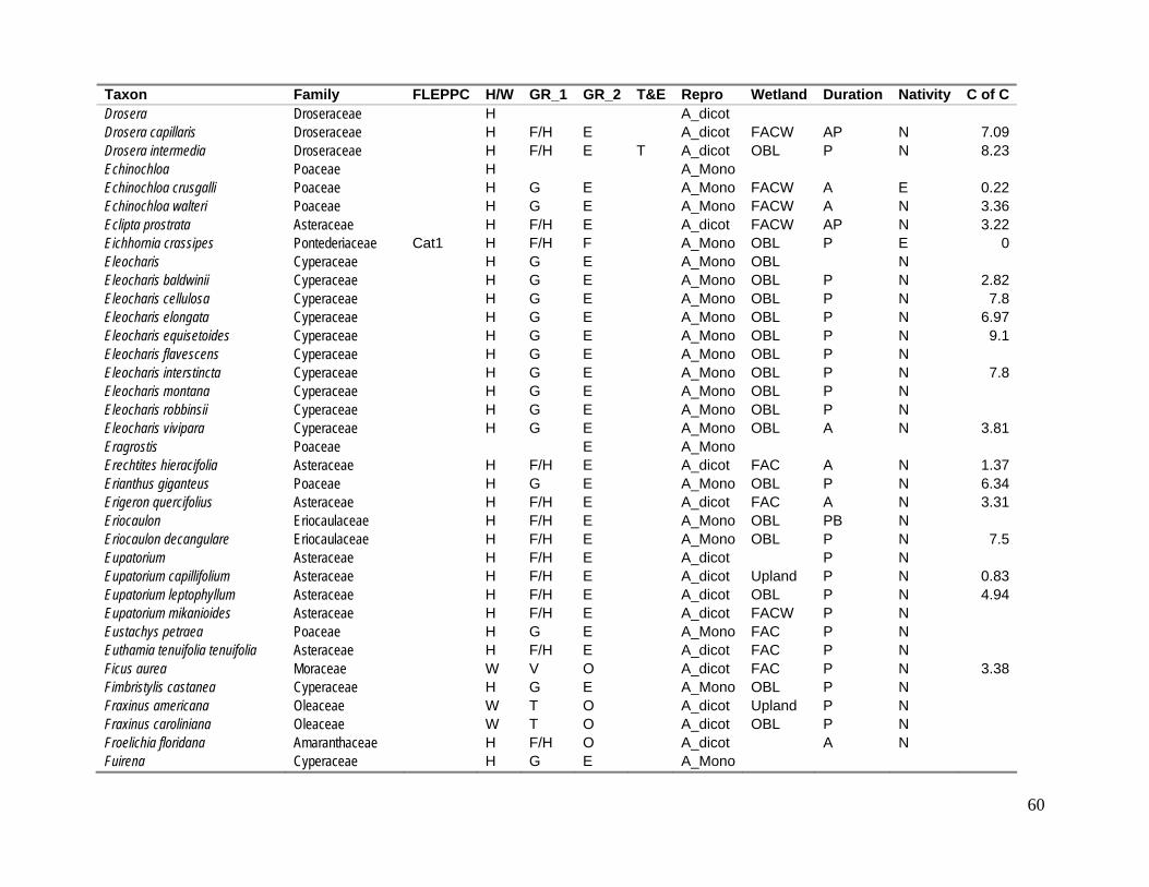
60

Taxon Family FLEPPC H/W GR_1 GR_2 T&E Repro Wetland Duration Nativity C of CDrosera Droseraceae H A_dicot Drosera capillaris Droseraceae H F/H E A_dicot FACW AP N 7.09Drosera intermedia Droseraceae H F/H E T A_dicot OBL P N 8.23Echinochloa Poaceae H A_Mono Echinochloa crusgalli Poaceae H G E A_Mono FACW A E 0.22Echinochloa walteri Poaceae H G E A_Mono FACW A N 3.36Eclipta prostrata Asteraceae H F/H E A_dicot FACW AP N 3.22Eichhornia crassipes Pontederiaceae Cat1 H F/H F A_Mono OBL P E 0Eleocharis Cyperaceae H G E A_Mono OBL N Eleocharis baldwinii Cyperaceae H G E A_Mono OBL P N 2.82Eleocharis cellulosa Cyperaceae H G E A_Mono OBL P N 7.8Eleocharis elongata Cyperaceae H G E A_Mono OBL P N 6.97Eleocharis equisetoides Cyperaceae H G E A_Mono OBL P N 9.1Eleocharis flavescens Cyperaceae H G E A_Mono OBL P N Eleocharis interstincta Cyperaceae H G E A_Mono OBL P N 7.8Eleocharis montana Cyperaceae H G E A_Mono OBL P N Eleocharis robbinsii Cyperaceae H G E A_Mono OBL P N Eleocharis vivipara Cyperaceae H G E A_Mono OBL A N 3.81Eragrostis Poaceae E A_Mono Erechtites hieracifolia Asteraceae H F/H E A_dicot FAC A N 1.37Erianthus giganteus Poaceae H G E A_Mono OBL P N 6.34Erigeron quercifolius Asteraceae H F/H E A_dicot FAC A N 3.31Eriocaulon Eriocaulaceae H F/H E A_Mono OBL PB N Eriocaulon decangulare Eriocaulaceae H F/H E A_Mono OBL P N 7.5Eupatorium Asteraceae H F/H E A_dicot P N Eupatorium capillifolium Asteraceae H F/H E A_dicot Upland P N 0.83Eupatorium leptophyllum Asteraceae H F/H E A_dicot OBL P N 4.94Eupatorium mikanioides Asteraceae H F/H E A_dicot FACW P N Eustachys petraea Poaceae H G E A_Mono FAC P N Euthamia tenuifolia tenuifolia Asteraceae H F/H E A_dicot FAC P N Ficus aurea Moraceae W V O A_dicot FAC P N 3.38Fimbristylis castanea Cyperaceae H G E A_Mono OBL P N Fraxinus americana Oleaceae W T O A_dicot Upland P N Fraxinus caroliniana Oleaceae W T O A_dicot OBL P N Froelichia floridana Amaranthaceae H F/H O A_dicot A N Fuirena Cyperaceae H G E A_Mono

61

Taxon Family FLEPPC H/W GR_1 GR_2 T&E Repro Wetland Duration Nativity C of CFuirena breviseta Cyperaceae H G E A_Mono OBL P N 7.6Fuirena pumila Cyperaceae H G E A_Mono OBL A N 5.92Fuirena scirpoidea Cyperaceae H G E A_Mono OBL P N 6.5Fuirena squarrosa Cyperaceae H G E A_Mono OBL P N Gleditsia triacanthus Fabaceae W T O A_dicot FACW P N Gordonia lasianthus Theaceae W T O A_dicot FACW P N 9.03Habenaria repens Orchidaceae H F/H E A_Mono FACW P N 4.58Hedyotis Rubiaceae Hibiscus coccineus Malvaceae H F/H E A_dicot OBL P N Hibiscus furcellatus Malvaceae SSH E A_dicot P N Hibiscus grandiflorus Malvaceae H F/H O A_dicot OBL P N 6.86Hydrilla verticillata Hydrocharitaceae Cat1 H F/H S A_Mono OBL P E 0Hydrocotyle Umbelliferae A_dicot Hydrocotyle umbellata Umbelliferae H F/H E A_dicot FACW P N 1.92Hydrolea corymbosa Hydrophyllaceae H F/H E A_dicot OBL P N 5.85Hydrolea quadrivalvis Hydrophyllaceae H F/H E A_dicot OBL P N Hypericum Clusiaceae A_dicot N Hypericum cistifolium Clusiaceae W SH O A_dicot FACW P N 6.32Hypericum fasciculatum Clusiaceae W SH O A_dicot OBL P N 7.27Hypericum hypericoides Clusiaceae W SH O A_dicot FAC P N 5.44Hypericum lissophloeus Clusiaceae W SH O E A_dicot OBL P N Hyptis alata Lamiaceae H F/H E A_dicot FACW P N 4.58Ilex cassine Aquifoliaceae W T O A_dicot OBL P N 7.66Ilex coriacea Aquifoliaceae W T O A_dicot FACW P N Ilex glabra Aquifoliaceae W SH O A_dicot FACW P N 5.85Ilex myrtifolia Aquifoliaceae W SH O A_dicot OBL P N Ilex vomitoria Aquifoliaceae W T O A_dicot FAC P N Indigofera hirsuta Leguminosae H F/H E A_dicot A E Ipomoea sagittata Convolvulaceae H V O A_dicot P N 6.42Iris hexagona Iridaceae H F/H E A_Mono OBL P N 6.97Iris virginica Iridaceae H F/H E A_Mono OBL P N Itea virginica Saxifragaceae W SH O A_dicot OBL P N 7.09Iva microcephala Asteraceae H F/H E A_dicot FACW A N 4.68Juncus Juncaceae H G A_Mono N Juncus effusus Juncaceae H G E A_Mono OBL P N 3.25Juncus marginatus Juncaceae H G E A_Mono FACW P N 3.65

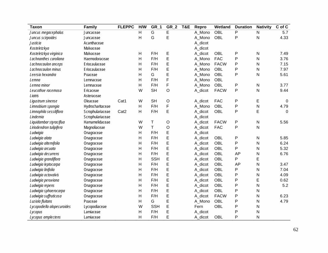
62

Taxon Family FLEPPC H/W GR_1 GR_2 T&E Repro Wetland Duration Nativity C of CJuncus megacephalus Juncaceae H G E A_Mono OBL P N 5.7Juncus scirpoides Juncaceae H G E A_Mono OBL P N 4.33Justicia Acanthaceae A_dicot Kosteletzkya Malvaceae A_dicot Kosteletzkya virginica Malvaceae H F/H E A_dicot OBL P N 7.49Lachnanthes caroliana Haemodoraceae H F/H E A_Mono FAC P N 3.76Lachnocaulon anceps Eriocaulaceae H F/H E A_Mono FACW P N 7.15Lachnocaulon minus Eriocaulaceae H F/H E A_Mono OBL P N 7.97Leersia hexandra Poaceae H G E A_Mono OBL P N 5.61Lemna Lemnaceae H F/H F A_Mono OBL Lemna minor Lemnaceae H F/H F A_Mono OBL P N 3.77Leucothoe racemosa Ericaceae W SH O A_dicot FACW P N 9.44Liatris Asteraceae Ligustrum sinense Oleaceae Cat1 W SH O A_dicot FAC P E 0Limnobium spongia Hydrocharitaceae H F/H F A_Mono OBL P N 4.79Limnophila sessiliflora Scrophulariaceae Cat2 H F/H E A_dicot OBL P E 0Lindernia Scrophulariaceae A_dicot Liquidambar styraciflua Hamamelidaceae W T O A_dicot FACW P N 5.56Liriodendron tulipifera Magnoliaceae W T O A_dicot FAC P N Ludwigia Onagraceae H F/H E A_dicot Ludwigia alata Onagraceae H F/H E A_dicot OBL P N 5.85Ludwigia alternifolia Onagraceae H F/H E A_dicot OBL P N 6.24Ludwigia arcuata Onagraceae H F/H E A_dicot OBL P N 5.32Ludwigia decurrens Onagraceae H F/H E A_dicot OBL AP N 6.76Ludwigia grandiflora Onagraceae H SSH E A_dicot OBL P E Ludwigia leptocarpa Onagraceae H F/H E A_dicot OBL AP N 3.47Ludwigia linifolia Onagraceae H F/H E A_dicot OBL P N 7.04Ludwigia octovalvis Onagraceae H F/H E A_dicot OBL P N 4.09Ludwigia peruviana Onagraceae H F/H E A_dicot OBL P E 0.62Ludwigia repens Onagraceae H F/H E A_dicot OBL P N 5.2Ludwigia sphaerocarpa Onagraceae H F/H E A_dicot OBL P N Ludwigia suffruticosa Onagraceae H F/H E A_dicot FACW P N 6.23Luziola fluitans Poaceae H G E A_Mono OBL P N 4.79Lycopodiella alopecuroides Lycopodiaceae W SSH E Fern OBL P N Lycopus Lamiaceae H F/H E A_dicot P N Lycopus amplectens Lamiaceae H F/H E A_dicot OBL P N

63

Taxon Family FLEPPC H/W GR_1 GR_2 T&E Repro Wetland Duration Nativity C of CLycopus virginicus Lamiaceae H F/H E A_dicot OBL P N Lygodium microphyllum Schizaeaceae Cat1 H V O Fern P E 0Lyonia Ericaceae A_dicot Lyonia lucida Ericaceae W SH O A_dicot FACW P N 7.06Magnolia grandiflora Magnoliaceae W T O A_dicot FAC P N Magnolia virginiana Magnoliaceae W T O A_dicot FACW P N 9.44Mayaca fluviatilis Mayacaceae H F/H S A_Mono OBL P N 8.45Melaleuca Myrtaceae W T O A_dicot Melaleuca quinquenervia Myrtaceae Cat1 W T O A_dicot FAC P E 0Melia azedarach Meliaceae Cat1 W T O A_dicot P E 0Micranthemum glomeratum Scrophulariaceae H F/H E A_dicot OBL P N 5.85Micranthemum umbrosum Scrophulariaceae H F/H E A_dicot OBL AP N 5.66Mikania scandens Asteraceae H V O A_dicot FACW P N 1.95Mimosa pigra Leguminosae Cat1 W T O A_dicot FAC P E 0Muhlenbergia capillaris Poaceae H G E A_Mono Upland P N Musa Musaceae E A_Mono Musa sapientum Musaceae T O A_Mono Upland P E Myrica cerifera Myricaceae W SH O A_dicot FAC P N 3.82Myriophyllum Haloragaceae H F/H S A_dicot OBL P Myriophyllum aquaticum Haloragaceae H F/H S A_dicot OBL P E 0.98Myriophyllum heterophyllum Haloragaceae H F/H S A_dicot OBL P N 4.77Najas gracillima Najadaceae H F/H S A_Mono OBL A N Najas guadalupensis Najadaceae H F/H S A_Mono OBL A N 5.07Najas minor Najadaceae H F/H S A_Mono OBL A E 3.64Nelumbo Nelumbonaceae H A_dicot Nelumbo lutea Nelumbonaceae H F/H F A_dicot OBL P N 6.26Nephrolepis Polypodiaceae Nitella Characeae NV S Algae N 7.28Nuphar luteum Nymphaeaceae H F/H F A_dicot OBL P N 4.64Nymphaea Nymphaeaceae H A_dicot Nymphaea mexicana Nymphaeaceae H F/H F A_dicot OBL P N 8.61Nymphaea odorata Nymphaeaceae H F/H F A_dicot OBL P N 7.18Nymphoides aquatica Menyanthaceae H F/H F A_dicot OBL P N 6.09Nyssa sylvatica biflora Cornaceae W T O A_dicot OBL P N 9.04Osmunda Osmundaceae E Fern Osmunda cinnamomea Osmundaceae H F/H E Fern FACW P N 6.44

64

Taxon Family FLEPPC H/W GR_1 GR_2 T&E Repro Wetland Duration Nativity C of COsmunda regalis Osmundaceae H F/H E Fern OBL P N 8.04Ostrya virginiana Betulaceae W T O A_dicot Upland P N Panicum Poaceae H G E A_Mono Panicum dichotomiflorum Poaceae H G E A_Mono FACW A N 4.96Panicum hemitomon Poaceae H G E A_Mono OBL P N 5.82Panicum repens Poaceae Cat1 H G E A_Mono FACW P E 0Panicum rigidulum Poaceae H G E A_Mono FACW P N 5.47Panicum rigidulum pubesens Poaceae H G E A_Mono OBL P N Panicum scabriusculum Poaceae H G E A_Mono OBL P N 7.15Panicum tenerum Poaceae H G E A_Mono OBL P N 8.67Panicum virgatum Poaceae H G E A_Mono FACW P N 5.44Paspalidium geminatum Poaceae H G E A_Mono OBL P N 6.36Paspalum Poaceae H G E A_Mono Paspalum distichum Poaceae H G E A_Mono OBL P N 5.54Paspalum floridanum Poaceae H G E A_Mono FACW P N 6.11Paspalum repens Poaceae H G E A_Mono OBL A N 6.69Paspalum urvillei Poaceae H G E A_Mono FAC P E 0Peltandra Araceae H F/H E A_Mono OBL P N 7.31Peltandra virginica Araceae H F/H E A_Mono OBL P N 7.31Pennisetum purpureum Poaceae Cat1 H G E A_Mono FAC P E 0Persea borbonia Lauraceae W T O A_dicot FACW P N 8.02Persea borbonia humilis Lauraceae W SH O A_dicot P N Persea palustris Lauraceae W T O A_dicot OBL P N 8.31Phanopyrum gymnocarpon Poaceae H G A_Mono OBL P N Phragmites australis Poaceae H F/H E A_Mono OBL P E 4.39Phyla nodiflora Verbenaceae H F/H E A_dicot FAC P N 1.92Pinus Pinaceae W T O Gymno Pinus clausa Pinaceae W T O Gymno FACW P N Pinus elliottii Pinaceae W T O Gymno P N 4.21Pinus palustris Pinaceae W T O Gymno P N 4.77Pistia stratiotes Araceae Cat1 H F/H F A_Mono OBL P E 0Pluchea Asteraceae H F/H E A_dicot FACW N Pluchea foetida Asteraceae H F/H E A_dicot FACW P N 6.65Pluchea odorata Asteraceae H F/H E A_dicot FACW AP N 4.96Pluchea rosea Asteraceae H F/H E A_dicot FACW P N 5.45Poaceae Poaceae

65

Taxon Family FLEPPC H/W GR_1 GR_2 T&E Repro Wetland Duration Nativity C of CPolygonum Polygonaceae H F/H E A_dicot Polygonum densiflorum Polygonaceae H F/H E A_dicot OBL AP N 5.32Polygonum hydropiperoides Polygonaceae H F/H E A_dicot OBL P N 4.02Polygonum punctatum Polygonaceae H F/H E A_dicot OBL AP N 4.02Polypogon monspeliensis Poaceae H G E A_Mono FAC A E Pontederia cordata Pontederiaceae H F/H E A_Mono OBL P N 5.38Pontederia rotundifolia Pontederiaceae H F/H E A_Mono P E Potamogeton diversifolius Potamogetonaceae H F/H S A_Mono OBL P N 7.15Potamogeton illinoensis Potamogetonaceae H F/H S A_Mono OBL P N 6.64Potamogeton pectinatus Potamogetonaceae H F/H S A_Mono OBL P N 7.8Potamogeton pusillus Potamogetonaceae H F/H S A_Mono OBL P N 7.8Quercus Fagaceae W T O A_dicot P N Quercus laurifolia Fagaceae W T O A_dicot FACW P N 5.14Quercus nigra Fagaceae W T O A_dicot FACW P N 4.14Rhexia Melastomataceae H F/H E A_dicot FACW P N Rhexia cubensis Melastomataceae H F/H E A_dicot FACW P N 7.22Rhexia mariana Melastomataceae H F/H E A_dicot FACW P N 5.5Rhexia nashii Melastomataceae H F/H E A_dicot FACW P N 7.8Rhexia virginica Melastomataceae H F/H E A_dicot FACW P N Rhus copallinum Anacardiaceae W SH O A_dicot P N 3.65Rhynchospora Cyperaceae H G E A_Mono N Rhynchospora baldwinii Cyperaceae H G E A_Mono OBL AP N Rhynchospora cephalantha Cyperaceae H G E A_Mono OBL P N 6.19Rhynchospora fascicularis Cyperaceae H G E A_Mono FACW P N 5.92Rhynchospora globularis Cyperaceae H G E A_Mono FACW AP N Rhynchospora inundata Cyperaceae H G E A_Mono OBL P N 7.25Rhynchospora microcarpa Cyperaceae H G E A_Mono OBL P N 5.29Rhynchospora microcephala Cyperaceae H G E A_Mono FACW P N 6.5Rhynchospora nitens Cyperaceae H G E A_Mono OBL AP N 5.2Rhynchospora scirpoides Cyperaceae H G E A_Mono OBL A N Rhynchospora tracyi Cyperaceae H G E A_Mono OBL P N 9.03Rubus Rosaceae H SH O A_dicot P N Rubus argutus Rosaceae H SH O A_dicot FAC P N 3.56Rubus trivialis Rosaceae H SH O A_dicot FAC P N 2.6Sabal palmetto Palmae W T O A_Mono FAC P N 4.85Sabatia grandiflora Gentianaceae H F/H E A_dicot FACW A N 7.09

66

Taxon Family FLEPPC H/W GR_1 GR_2 T&E Repro Wetland Duration Nativity C of CSaccharum Poaceae H G E A_Mono Sacciolepis striata Poaceae H G E A_Mono OBL P N 5.35Sagittaria Alismataceae H F/H A_Mono OBL P N Sagittaria graminea Alismataceae H F/H E A_Mono OBL P N 5.53Sagittaria kurziana Alismataceae H F/H S A_Mono OBL P N 9.75Sagittaria lancifolia Alismataceae H F/H E A_Mono OBL P N 4.96Sagittaria latifolia Alismataceae H F/H E A_Mono OBL P N 6.5Sagittaria subulata Alismataceae H F/H E A_Mono OBL P N Salix Salicaceae W A_dicot Salix babylonica Salicaceae W T O A_dicot OBL P E Salix caroliniana Salicaceae W T O A_dicot OBL P N 2.95Salix eriocephala Salicaceae W T O E A_dicot FACW P N Salix floridana Salicaceae W T O E A_dicot FACW P N Salvinia minima Salviniaceae H F/H F Fern OBL AP E 2.03Sambucus Caprifoliaceae A_dicot Sambucus canadensis Caprifoliaceae W SH O A_dicot FAC P N 1.48Sapium sebiferum Euphorbiaceae Cat1 W T O A_dicot FAC P E 0Sarcostemma clausum Asclepiadaceae H V O A_dicot FACW P N 3.81Saururus cernuus Saururaceae H F/H E A_dicot OBL P N 7.33Schinus terebinthifolius Anacardiaceae Cat1 W T O A_dicot FAC P E 0Schizachyrium Poaceae A_Mono Scirpus Cyperaceae H G E A_Mono OBL P Scirpus americanus Cyperaceae H G E A_Mono OBL P N 6.5Scirpus californicus Cyperaceae H G E A_Mono OBL P N 6.01Scirpus cubensis Cyperaceae H G E A_Mono OBL P E 3.77Scirpus cyperinus Cyperaceae H G E A_Mono OBL P N Scirpus pungens Cyperaceae H G E A_Mono OBL P N Scirpus validus Cyperaceae H G E A_Mono OBL P N 5.55Scleria Cyperaceae H G E A_Mono Serenoa repens Palmae W SH O A_Mono Upland P N 7.03Sesbania Fabaceae A_dicot Sesbania herbacea Fabaceae H F/H E A_dicot FAC A N 1.5Sesbania punicea Fabaceae Cat2 W SH O A_dicot FAC P E 0Setaria magna Poaceae H G E A_Mono FACW A N Setaria parviflora Poaceae H G E A_Mono FAC P N 3.4Smilax Smilacaceae V O A_Mono P N

67

Taxon Family FLEPPC H/W GR_1 GR_2 T&E Repro Wetland Duration Nativity C of CSmilax laurifolia Smilacaceae V O A_Mono FACW P N Smilax pumila Smilacaceae V O A_Mono P N 6.01Solidago Asteraceae H F/H E A_dicot P N Solidago fistulosa Asteraceae H F/H E A_dicot FACW P N 4.49Solidago leavenworthii Asteraceae H F/H E A_dicot FAC P N Solidago stricta Asteraceae H F/H E A_dicot FACW P N 5.49Spartina alterniflora Poaceae H G E A_Mono OBL P N 7.94Spartina bakeri Poaceae H G E A_Mono FACW P N 5.98Spirodela polyrhiza Lemnaceae H F/H F A_Mono OBL P N 2.95Taxodium ascendens Taxodiaceae W T O Gymno OBL P N 7.21Taxodium distichum Taxodiaceae W T O Gymno OBL P N 7.21Thalia geniculata Marantaceae H F/H E A_Mono OBL P N 7.12Thelypteris Polypodiaceae E Fern Thelypteris interrupta Polypodiaceae H F/H E Fern FACW P N 6.74Toxicodendron Anacardiaceae A_dicot Toxicodendron radicans Anacardiaceae H V O A_dicot FAC P N 1.44Toxicodendron vernix Anacardiaceae W T O A_dicot OBL P N Tradescantia ohiensis Commelinaceae H F/H E A_Mono FAC P N Triadenum virginicum Clusiaceae H F/H E A_dicot OBL P N 8.16Typha Typhaceae H E A_Mono P N Typha domingensis Typhaceae H F/H E A_Mono OBL P N 0.59Typha latifolia Typhaceae H F/H E A_Mono OBL P N 1.6Ulmus americana Ulmaceae W T O A_dicot FACW P N 7.68Urena lobata Malvaceae Cat2 H SSH O A_dicot Upland P E 0Utricularia Lentibulariaceae H S Utricularia cornuta Lentibulariaceae H F/H S A_dicot OBL AP N 7.46Utricularia floridana Lentibulariaceae H F/H S A_dicot OBL P N 6.34Utricularia foliosa Lentibulariaceae H F/H S A_dicot OBL P N 6.44Utricularia gibba Lentibulariaceae H F/H S A_dicot OBL AP N 6.37Utricularia inflata Lentibulariaceae H F/H S A_dicot OBL P N 5.85Utricularia olivacea Lentibulariaceae H F/H S A_dicot OBL AP N Utricularia purpurea Lentibulariaceae H F/H S A_dicot OBL AP N 6.5Utricularia radiata Lentibulariaceae H F/H S A_dicot OBL AP N 6.01Utricularia subulata Lentibulariaceae H F/H S A_dicot OBL AP N 7.23Vallisneria americana Hydrocharitaceae H F/H S A_Mono OBL P N 7.28Verbena bonariensis Verbenaceae H F/H E A_dicot FAC APB E 0.56

68

Taxon Family FLEPPC H/W GR_1 GR_2 T&E Repro Wetland Duration Nativity C of CVigna luteola Fabaceae W V O A_dicot FACW P N Vitaceae Vitaceae Vitis Vitaceae H V O A_dicot Vitis rotundifolia Vitaceae H V O A_dicot FAC P N 1.18Websteria confervoides Cyperaceae H G S A_Mono OBL P N Wedelia trilobata Asteraceae Cat2 H F/H E A_dicot FAC AP E 0Wolffiella Lemnaceae H F/H F A_Mono OBL P N 4.37Woodwardia areolata Polypodiaceae H F/H E Fern OBL P N 7.68Woodwardia virginica Polypodiaceae H F/H E Fern FACW P N 6.5Xanthosoma sagittifolium Araceae Cat2 H F/H E A_Mono FACW P E 0Xyris Xyridaceae H F/H E A_Mono OBL P N Xyris baldwiniana Xyridaceae H F/H E A_Mono OBL P N 6.97Xyris fimbriata Xyridaceae H F/H E A_Mono OBL P N 7.08Xyris isoetifolia Xyridaceae H F/H E E A_Mono OBL P N Xyris smalliana Xyridaceae H F/H E A_Mono OBL P N 7.8Zanthoxylum Rutaceae Zizania aquatica Poaceae H G E A_Mono OBL A N 6.69Zizaniopsis miliacea Poaceae H G E A_Mono OBL P N 6.21

69

APPENDIX 2. EPA’S WETLAND PLANT ATTRIBUTES

Florida taxon name, the taxon’s general tolerance to pollution, nutrients, N, P, flooding, sediment, or salinity based on a national wetland database (Adamus and Gonyaw, 2000) (T = tolerant, M = moderately tolerant, V = very tolerant, S = sensitive).

Taxon GenPoll Nutrients N P Flooding Sediment Salinity

Acer rubrum T M T T T S Amorpha fruticosa M Andropogon virginicus T M M S Andropogon M Arundinaria gigantea M M S Aster pilosus T M M S Aster S Baccharis halimifolia M M T Bacopa monnieri T Bidens laevis M M M Bidens T Boehmeria cylindrica M M M S Brasenia schreberi M M M S Callitriche T T S Carex T T S S Carya aquatica T Catalpa M Cephalanthus occidentalis M M T S Ceratophyllum demersum M M T T VT S Chamaecyparis thyoides T M S Chara S T Cicuta maculata T M M S Cladium jamaicense T T T Conoclinium coelestinum M M S Cyperus erythrorhizos M Cyperus esculentus T M M S Cyperus odoratus M Cyperus rotundus T Decodon verticillatus M M M S Diospyros virginiana T M T T S Drosera intermedia S Echinochloa crusgalli T M M S Echinochloa walteri M Eichhornia crassipes M T T VT S Eleocharis elongata T Eleocharis interstincta T T T Eleocharis robbinsii M T Eleocharis T M Erechtites hieracifolia M M S Eupatorium S Fraxinus americana M M M S

70

Taxon GenPoll Nutrients N P Flooding Sediment Salinity

Fraxinus caroliniana T Gordonia lasianthus M Hydrilla verticillata T S Hydrocotyle umbellata S M M S Hypericum T S Ilex glabra M M S Iris virginica M Itea virginica M M S Juncus effusus T M M M Juncus marginatus M M M S Juncus S Leersia hexandra T Lemna minor M M T T T S Lemna T M T Leucothoe racemosa M M S Liquidambar styraciflua M T S Liriodendron tulipifera M M T S Ludwigia alternifolia M M M S Lycopus virginicus M M M S Lyonia lucida M M S Magnolia grandiflora M Magnolia virginiana M M S Melaleuca quinquenervia T Mikania scandens M T S Mimosa pigra T Myrica cerifera M M S Myriophyllum aquaticum VT T T S Myriophyllum heterophyllum

S T

Najas gracillima M Najas guadalupensis M Najas minor VT M T S Nelumbo lutea T M S Nuphar luteum M T Nymphaea odorata M M M S Osmunda cinnamomea M M M S Osmunda regalis M M M S Ostrya virginiana M M M S Panicum dichotomiflorum M Panicum hemitomon T Panicum virgatum M M M M Panicum T S Peltandra virginica M M T T M S Persea borbonia M Phragmites australis T VT T M S M Pinus elliottii S Polygonum densiflorum VT Polygonum hydropiperoides

M M T S

71

Taxon GenPoll Nutrients N P Flooding Sediment Salinity

Polygonum punctatum M M M M Pontederia cordata M M M S Potamogeton diversifolius M Potamogeton pectinatus T T T T T T Potamogeton pusillus T Quercus laurifolia M Quercus nigra T M T S Rhexia mariana M M S Rhexia virginica M M S Rhus copallinum S Rhynchospora inundata M M S Rubus S Sagittaria graminea M Sagittaria lancifolia T T Sagittaria latifolia M M M S Sagittaria M M S Salix babylonica VT M M S Salix eriocephala M Salix VT Sambucus canadensis M M M S S Sapium sebiferum VT Saururus cernuus M M M S Scirpus americanus M M T T Scirpus cyperinus M M M S Scirpus pungens M Scirpus validus M T M Solidago M Spartina alterniflora M T T T Spirodela polyrhiza T M T S Taxodium distichum M T S Toxicodendron vernix M M S Tradescantia ohiensis M Triadenum virginicum M M M S Typha domingensis T T T Typha latifolia T M T T T S Typha M T T M S Ulmus americana M M T S Utricularia cornuta T M S Utricularia gibba M Utricularia inflata M T S Utricularia purpurea M T S Utricularia subulata T Vallisneria americana M M T S S Vitis rotundifolia M M S Woodwardia areolata M M M S Woodwardia virginica S M M S Xyris smalliana T Xyris S Zizania aquatica M M T S

APPENDIX 3. RESULTS OF TESTING FOR TOLERANCE AND SENSITIVITY

List of lake taxa that occurred in >= 4 lakes (out of 95). Shown for each taxon are CC value, whether the taxon was defined as a sensitive or tolerant taxa on the basis of CC scores, number of lakes in which taxon was found, number of occurrences that were in minimally disturbed lakes (HDG < 3), whether the association with HDG was significant (χ2, * p < 0.05, * * p < 0.01), and whether the association was in the direction predicted.

Taxon CC Tol/Sens # Occur # Good Significant Correct

Bidens laevis 7.19 S 7 5 Blechnum serrulatum 7.15 S 13 6 Cephalanthus occidentalis 7.27 S 51 25 * yes Cladium jamaicense 9.04 S 22 15 * * yes Crinum americanum 8.67 S 5 2 Decodon verticillatus 7.80 S 12 10 * * yes Eleocharis cellulosa 7.80 S 13 3 Eleocharis interstincta 7.80 S 14 4 Gordonia lasianthus 9.03 S 11 7 Hypericum fasciculatum 7.27 S 13 10 * * yes Ilex cassine 7.66 S 37 18 Itea virginica 7.09 S 9 6 Lyonia lucida 7.06 S 8 7 * * yes Magnolia virginiana 9.44 S 42 18 Mayaca fluviatilis 8.45 S 19 12 * yes Nitella 7.28 S 11 2 Nymphaea odorata 7.18 S 43 22 * yes Nyssa sylvatica biflora 9.04 S 30 13 Osmunda regalis 8.04 S 7 4 Persea palustris 8.31 S 10 4 Potamogeton diversifolius 7.15 S 4 1 Rhynchospora inundata 7.25 S 8 5 Saururus cernuus 7.33 S 8 4 Serenoa repens 7.03 S 4 3 Taxodium ascendens 7.21 S 39 17 Taxodium distichum 7.21 S 34 9 Thalia geniculata 7.12 S 5 1 Triadenum virginicum 8.16 S 17 11 * yes Vallisneria americana 7.28 S 18 2 * no Woodwardia areolata 7.68 S 4 3 Alternanthera philoxeroides 0.00 T 49 10 * * yes Azolla caroliniana 1.81 T 6 2 Brachiaria mutica 0 T 18 2 * yes Centella asiatica 1.92 T 11 6 Colocasia esculenta 0 T 40 7 * * yes Cyperus alternifolius 1.11 T 9 1 Cyperus polystachyos 1.56 T 9 3 Cyperus surinamensis 2.03 T 14 1 * yes

73

Taxon CC Tol/Sens # Occur # Good Significant Correct

Eichhornia crassipes 0.00 T 25 10 Eleocharis baldwinii 2.82 T 50 23 Eupatorium capillifolium 0.83 T 59 20 Hydrilla verticillata 0.00 T 19 1 * * yes Hydrocotyle umbellata 1.92 T 62 20 Ludwigia peruviana 0.62 T 42 10 * yes Melaleuca quinquenervia 0.00 T 20 6 Mikania scandens 1.95 T 65 16 * * yes Myriophyllum aquaticum 0.98 T 5 0 Panicum repens 0 T 73 23 * yes Pistia stratiotes 0 T 15 1 * yes Salix caroliniana 2.95 T 61 19 Salvinia minima 2.03 T 34 9 Sambucus canadensis 1.48 T 12 1 Sapium sebiferum 0 T 21 3 * yes Schinus terebinthifolius 0.00 T 34 6 * * yes Typha domingensis 0.59 T 15 4 Typha latifolia 1.60 T 55 16 Vitis rotundifolia 1.18 T 16 6 Wedelia trilobata 0 T 9 1 Acer rubrum 4.65 67 24 Andropogon na 11 7 Andropogon glomeratus 3.90 20 8 Andropogon virginicus 3.44 9 5 Aster na 4 2 Aster carolinianus na 6 2 Aster subulatus 5.74 5 3 Baccharis na 6 2 Baccharis glomeruliflora 6.12 16 6 Bacopa caroliniana 5.31 9 6 Bacopa monnieri 4.49 11 3 Bidens na 25 10 Bidens mitis 6.31 5 4 Blechnum na 7 2 Boehmeria cylindrica 5.91 19 8 Cabomba caroliniana 5.07 9 7 * unknown Canna flaccida 6.75 7 1 Casuarina equisetifolia 0 4 0 Ceratophyllum demersum 4.16 7 1 Chara 3.90 15 2 Cicuta maculata na 5 2 Cyperus na 23 5 Cyperus haspan 5.68 17 7 Cyperus lecontei na 8 3 Cyperus odoratus 4.25 27 3 * * unknown Cyrilla racemiflora 5.20 14 8 Echinochloa na 5 0 Echinochloa walteri 3.36 5 3 Eleocharis na 9 3

74

Taxon CC Tol/Sens # Occur # Good Significant Correct

Eriocaulon na 7 5 Eupatorium na 14 6 Eupatorium leptophyllum 4.94 4 2 Fuirena na 7 2 Fuirena scirpoidea 6.50 21 9 Habenaria repens 4.58 6 4 Hydrocotyle na 17 5 Hypericum na 6 5 Juncus na 7 5 Juncus effusus 3.25 12 6 Juncus marginatus 3.65 5 0 Juncus megacephalus 5.70 4 3 Lachnanthes caroliana 3.76 24 16 * * unknown Leersia hexandra 5.61 8 5 Lemna minor 3.77 19 6 Limnobium spongia 4.79 5 3 Liquidambar styraciflua 5.56 13 7 Ludwigia na 25 10 Ludwigia alata 5.85 4 4 * yes Ludwigia arcuata 5.32 6 3 Ludwigia grandiflora na 7 2 Ludwigia leptocarpa 3.47 25 5 Ludwigia octovalvis 4.09 39 10 Ludwigia repens 5.20 9 4 Ludwigia suffruticosa 6.23 6 5 Luziola fluitans 4.79 10 6 Lycopus na 4 2 Lycopus virginicus na 5 3 Magnolia grandiflora na 8 6 Melaleuca na 7 0 Micranthemum umbrosum 5.66 7 2 Musa na 5 0 Myrica cerifera 3.82 76 28 Myriophyllum heterophyllum 4.77 4 3 Najas guadalupensis 5.07 7 2 Nelumbo lutea 6.26 8 3 Nuphar luteum 4.64 63 25 Nymphoides aquatica 6.09 17 13 * * yes Osmunda cinnamomea 6.44 9 4 Panicum na 5 3 Panicum hemitomon 5.82 70 28 Paspalidium geminatum 6.36 9 1 Paspalum na 4 2 Paspalum repens 6.69 6 1 Phragmites australis 4.39 15 4 Pinus elliottii 4.21 26 13 Pluchea na 7 2 Pluchea foetida 6.65 5 3 Pluchea odorata 4.96 8 3

75

Taxon CC Tol/Sens # Occur # Good Significant Correct

Pluchea rosea 5.45 8 5 Polygonum na 12 4 Polygonum densiflorum 5.32 21 5 Polygonum hydropiperoides 4.02 23 9 Polygonum punctatum 4.02 6 2 Pontederia cordata 5.38 64 25 Potamogeton illinoensis 6.64 8 1 Quercus laurifolia 5.14 9 1 Quercus nigra 4.14 4 1 Rhynchospora na 10 5 Rhynchospora nitens 5.20 5 2 Rubus na 4 3 Sabal palmetto 4.85 9 2 Sacciolepis striata 5.35 40 15 Sagittaria lancifolia 4.96 44 16 Sagittaria latifolia 6.50 14 4 Sagittaria subulata na 4 2 Salix na 10 3 Sambucus na 7 1 Sarcostemma clausum 3.81 9 2 Scirpus californicus 6.01 10 3 Scirpus cubensis 3.77 15 3 Scirpus cyperinus na 4 4 * unknown Scirpus validus 5.55 10 1 Sesbania na 5 2 Solidago na 17 12 * * unknown Spartina bakeri 5.98 7 2 Thelypteris na 4 3 Typha na 9 3 Utricularia na 18 11 * unknown Utricularia floridana 6.34 6 3 Utricularia gibba 6.37 10 4 Utricularia purpurea 6.50 7 6 * yes Vitis na 4 2 Woodwardia virginica 6.50 11 6 Xyris na 26 13 Zizaniopsis miliacea 6.21 5 2

APPENDIX 4. LVI VALUES BY DISTRICT

Lake district, water body name, nick name, county, HDG, and LVI (average of 12 replicates) for the 95 lakes used to develop and test the LVI.

District Waterbody name Nick name County STORET HDG LVI_1x

Central Russell Lake OSCEO78 Osceola 26010239 2 61.81Central Holden Lake ORANG159 Orange 26010884 5 23.07Central Lake Barton LakeBarton Orange 20010890 5 35.50Central Lake Rexford REXFORDUNK Orange 26010012 5 47.16Central Downey Lake ORANG44 Orange 20010319 3 63.91Central Halfmoon Lake HALFMN*REF Marion 20020463 1 74.47Central Winona Lake LKWINONA Lake 20020470 4 32.05Central Davis Lake LKDAVIS Lake 20030148 3 62.69Central Lake Norris LKNORRIS Lake 20010355 3 64.00Central Hammond Lake HAMMONDREF Lake 20020014 1 80.22Central Sellers Lake SELLCTREF Lake 20020496 0 84.42Central Grasshopper Lake GRAHOP*REF Lake 20030913 1 90.97Northeast Butler Lake UNION8 Union 21030015 2 59.52Northeast Swift Creek Pond SFPNDCTREF Union 21030066 0 81.17Northeast Louise Lake SUWAN4 Suwannee 21020016 3 46.97Northeast Lake Ida LKIDA Putnam 20020116 4 42.71Northeast Lake Fanny LKFANNY Putnam 20020100 1 74.08Northeast Lake Fanny LKFANNY Putnam 20020100 1 89.79Northeast Cherry Lake CHERYNEUNK Madison 21010039 2 53.57Northeast Cherry Lake CHERYNEUNK Madison 21010039 2 61.60Northeast Francis Lake FRANTST Madison 21020056 5 69.36Northeast Lake Mystic MYSTICREF Madison 22040025 1 82.11Northeast Dead Lake CRESTUDY4 Flagler 20030461 3 49.76Northeast Gore Lake GOREREF Flagler 20030339 2 74.60Northeast Tank Lake TANKLAKE Flagler 20030151 1 96.84Northeast Watertown Lake WATERTWNLK Columbia 21010206 3 49.65Northeast Magnolia Lake MAGNOLREF Clay 20030545 1 72.00Northeast Rowell Lake ROWELLCT Bradford 21030110 4 38.97Northeast Lake Altho LKALTHO Alachua 21030047 2 77.47Northwest Rattlesnake Lake RSNAKEREF Washington 32030099 0 69.45Northwest Porter Lake PORTERREF Washington 32030097 0 82.83Northwest Porter Lake PORTERREF Washington 32030097 1 84.80Northwest Otter Lake OTTER*REF Wakulla 22020090 1 68.79Northwest Bear Lake BEARTST Santa Rosa 33030057 4 51.47Northwest Kell-Air Lake KELLALK Okaloosa 32010050 7 14.63Northwest Karick Lake KARICKTST Okaloosa 33040042 5 65.32Northwest Lake Munson LKMUNSON Leon 23010165 6 22.98Northwest Lake Victor LKVICTOR Holmes 32010085 5 37.78Northwest Sand Hammock Pond SANDPOND Holmes 32010038 2 78.47Northwest Lake Cassidy CASSCTREF Holmes 32020104 0 80.73Northwest Stone Lake LKSTONE Escambia 33020097 3 34.99Northwest Court Martial Lake CORTMARREF Bay 32030098 1 71.78

77

District Waterbody name Nick name County STORET HDG LVI_1x

South Lake Verona LKVERONMID Highlands 26010339FTM 4 28.75South Lake Pioneer LKPIONEER Highlands 26010651FTM 7 30.48South Lake Tulane LKTULANMID Highlands 26010340FTM 5 31.25South Lake Carrie LKCARRIE Highlands 26010585 7 36.78South Lake Denton LKDENTON Highlands 26010648 4 39.52South Lake Viola VIOLCTREF Highlands 26010605 7 41.41South June In Winter Lake HIGHL73 Highlands 26010559 6 47.56South Lake Placid LKPLACIDNO Highlands 26010650FTM 4 48.91South Wolf Lake WOLFCTREF Highlands 26010613 4 50.55South Lake Little Bonnet LTLBONNET Highlands 26010326 3 50.95South Lake Olivia LKOLIVIA Highlands 26010652FTM 6 51.05South Red Beach Lake REDBCHREF Highlands 26010638 4 53.63South Lake Apthorpe APTHORPREF Highlands 26010630 3 57.85South Persimmon Lake HIGHL11 Highlands 26010303 5 58.12South Annie Lake ANNMIDREF Highlands 26010310 0 81.23South Submarine Lake SUBMARIREF Highlands 26010640 2 83.72South Little Lake LITTLE REF Highlands 26010636 2 87.82South Lake Yellowhammer LKYELHAM Charlotte 25010080FTM 3 41.53South Lake Webb LKWEBB Charlotte 25010079 2 61.66Southeast Lake At Tozour Rd. LKTOZOUR St Lucie 28010596 4 38.79Southeast Lake Eden LKEDEN St Lucie 28010595 1 52.13Southeast Lake Ida Pb LAKEIDA Palmbeach 28010500 5 9.61Southeast Lake Osborne LKOSBORNE Palmbeach 28010500 7 11.82Southeast Lake Clark LKCLARK Palmbeach 28010400 6 13.43Southeast Wellington Lake LKWELNGTON Palmbeach 28010600 6 41.58Southeast Lake Halpatioke LKHALPATOK Martin 28010594 0 47.91Southeast Quiet Waters Lake N LKQUIETH2O Broward 28030600 2 46.49Southwest Lake Deaton L58P Sumter UNKNOWNL58P 1 54.21Southwest Banana Lake L84-BANANA Polk 27584418154127 4 18.74Southwest Lake Conine CONINETST Polk 25020131 5 31.26Southwest Lake Lena L74-LENA Polk 28040038148367 6 42.36Southwest Lake Mattie MATTIE1REF Polk 23010406 2 43.98Southwest Lake Elbert LKELBERT Polk 28013598142314 5 44.95Southwest Lake Rochelle SWDLL1027 Polk 14580 4 46.00Southwest Lake Daisy LKDAISY Polk 27594708139333 5 49.41Southwest Lake Juliana JULIANREF Polk 23010427 5 49.47Southwest Lake Martha LKMARTHA Polk 25020198 5 49.71Southwest Lake Shipp LKSHIPP Polk 25020355 7 49.99Southwest Lake Martha LKMARTHA Polk 25020198 5 51.62Southwest Lake Easy L53PEASY Polk 25023002 1 54.88Southwest Lake Annie LAKE ANNIE Polk 27594380813618 2 55.66Southwest East Lake L51PEAST Pasco 24040806 3 26.78Southwest Lake Como L61PCOMO Pasco 24040805 6 51.83Southwest Lake Walden L52PWALDEN Hillsborough 24040170 3 9.12Southwest Lake Weeks WEEKSREF Hillsborough 24030082 5 23.96Southwest Lake Norbert LKNORBERT Hillsborough 28091278228372 4 25.04Southwest Lake Bellows LKBELLOS Hillsborough 24030127 5 29.08Southwest Lake Le Clare LKLECLARE Hillsborough 28063598232193 2 29.33Southwest Thonotosassa Lake THONOTST Hillsborough 24030022 5 30.55

78

District Waterbody name Nick name County STORET HDG LVI_1x

Southwest White Trout Lake L62P Hillsborough UNKNOWNL62P 3 40.48Southwest Lake Williams LKWILLIAMS Hillsborough 28055458236093 4 51.66Southwest Lake Brooker L59PBRKR Hillsborough 24040172 4 53.85Southwest Lake Alice ALICEPREF Hillsborough 24040019 2 68.19Southwest Lake Rogers L63P Hillsborough UNKNOWNL63P 1 71.24Southwest Spring Lake L65P Hernando UNKNOWNL65P 4 46.37Southwest Lake Lindsey LKLINDSY Hernando 23010439 2 66.78Southwest Lake Tooke TOOKEPREF Hernando 24040015 2 67.21Southwest Lake Tooke TOOKEPREF Hernando 24040015 1 74.54

79

APPENDIX 5. ADDITIONAL TABLES

App. Table 5.1. Details for Table 4 including N, Spearman’s r, and associated p level.

Disturbance measures N r p-level

HDG & WQ index 91 0.62 0.00

HDG & LDI 98 0.73 0.00

HDG & Habitat index 95 -0.87 0.00

WQ index & HDG 91 0.62 0.00

WQ index & LDI 91 0.19 0.07

WQ index & Habitat index 87 -0.46 0.00

LDI & HDG 98 0.73 0.00

LDI & WQ index 91 0.19 0.07

LDI & Habitat index 93 -0.69 0.00

Habitat index & HDG 95 -0.87 0.00

Habitat index & WQ index 87 -0.46 0.00

Habitat index & LDI 93 -0.69 0.00

80

App. Table 5.2. Candidate plant metrics and their correlation with HDG, the WQ index, LDI, and the habitat index, detail from Table 6. The sample size is shown for all metrics except dominant C of C for which N ranged from 57–65. Most metrics were calculated as both the total number of taxa and the percentage of total taxa (left vs. right side of table); exceptions to this were metrics in the category “Community structure” which could only be calculated in one way.

Number of taxa Percent of total taxa HDG WQ LDI Hab HDG WQ LDI Hab

N = 95 95 93 90 95 95 93 90 Community structure Total taxa -0.05 0.04 -0.17 0.16 - - - - No. of plant guilds 0.25 0.15 0.07 -0.15 - - - - Dominant C of C -0.52 -0.43 0.49 - - - - Nativity Native -0.24 -0.13 -0.31 0.35 -0.56 -0.46 -0.53 0.64 Invasive 0.55 0.50 0.45 -0.48 0.63 0.51 0.61 -0.65 Category 1 0.56 0.44 0.48 -0.50 0.58 0.43 0.58 -0.58 Categories 1 & 2 0.59 0.51 0.49 -0.53 0.62 0.48 0.60 -0.62 Tolerance FQI SCORE -0.52 -0.32 -0.54 0.57 - - - - Average C of C -0.67 -0.49 -0.59 0.63 - - - - Sensitive (CC>7) -0.40 -0.31 -0.41 0.46 -0.49 -0.44 -0.41 0.48 Tolerant (CC<3) 0.48 0.39 0.35 -0.37 0.67 0.42 0.60 -0.59 V. Tolerant (CC<2) 0.51 0.40 0.38 -0.40 0.65 0.41 0.59 -0.59 Duration Perennial -0.07 -0.01 -0.16 0.18 -0.08 -0.15 -0.01 0.15 Annual -0.15 0.12 -0.31 0.26 -0.16 0.09 -0.32 0.25 Annual:Perennial ratio 0.11 0.18 0.10 0.02 -0.12 0.14 -0.27 0.21 Native perennials -0.24 -0.16 -0.32 0.35 -0.07 -0.07 -0.08 0.07 Native annuals 0.00 0.16 -0.05 0.14 0.16 0.24 0.14 -0.04 Wetland status Obligate wetland -0.06 0.11 -0.15 0.17 -0.02 0.23 0.00 0.04 Obl. & Facult. -0.03 0.08 -0.14 0.17 0.07 0.20 0.00 0.07 Upland 0.07 -0.10 0.01 0.04 0.09 -0.14 0.04 -0.01 Native obl. Wetland -0.20 -0.03 -0.26 0.31 0.01 0.23 0.09 -0.06 Native facult wetland -0.03 -0.09 -0.11 0.17 0.23 -0.01 0.15 -0.12 Native upland 0.00 -0.15 -0.08 0.13 0.12 -0.11 0.04 -0.02 Growth form Herbaceous 0.02 0.09 -0.07 0.12 0.14 0.18 0.24 -0.11 Woody -0.18 -0.11 -0.31 0.21 -0.18 -0.21 -0.25 0.15 Emergent 0.01 0.07 -0.09 0.14 0.18 0.15 0.14 -0.09 Floating -0.04 0.20 -0.05 0.04 -0.03 0.18 0.06 -0.03 Submersed 0.05 -0.18 0.19 -0.07 0.05 -0.19 0.23 -0.09 Fern -0.08 0.16 -0.27 0.21 -0.06 0.14 -0.23 0.19 Gymnosperm 0.07 -0.06 0.01 0.00 0.06 -0.12 0.05 -0.03 Native herbaceous -0.14 -0.07 -0.17 0.29 0.13 0.11 0.29 -0.10 Native woody -0.32 -0.14 -0.48 0.37 -0.13 -0.08 -0.29 0.13 Native emergent -0.14 -0.03 -0.21 0.31 0.11 0.17 0.14 -0.02 Native floating -0.28 -0.16 -0.14 0.19 -0.22 -0.17 -0.02 0.09

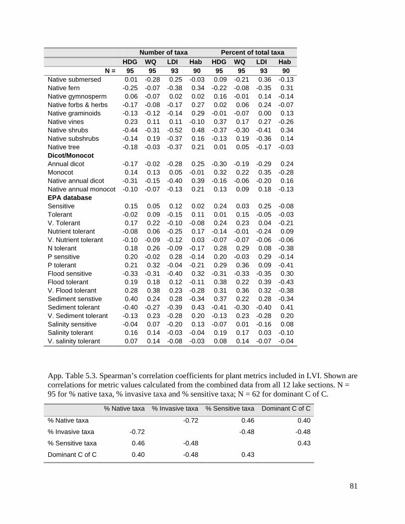
81

Number of taxa Percent of total taxa HDG WQ LDI Hab HDG WQ LDI Hab

N = 95 95 93 90 95 95 93 90 Native submersed 0.01 -0.28 0.25 -0.03 0.09 -0.21 0.36 -0.13 Native fern -0.25 -0.07 -0.38 0.34 -0.22 -0.08 -0.35 0.31 Native gymnosperm 0.06 -0.07 0.02 0.02 0.16 -0.01 0.14 -0.14 Native forbs & herbs -0.17 -0.08 -0.17 0.27 0.02 0.06 0.24 -0.07 Native graminoids -0.13 -0.12 -0.14 0.29 -0.01 -0.07 0.00 0.13 Native vines 0.23 0.11 0.11 -0.10 0.37 0.17 0.27 -0.26 Native shrubs -0.44 -0.31 -0.52 0.48 -0.37 -0.30 -0.41 0.34 Native subshrubs -0.14 0.19 -0.37 0.16 -0.13 0.19 -0.36 0.14 Native tree -0.18 -0.03 -0.37 0.21 0.01 0.05 -0.17 -0.03 Dicot/Monocot Annual dicot -0.17 -0.02 -0.28 0.25 -0.30 -0.19 -0.29 0.24 Monocot 0.14 0.13 0.05 -0.01 0.32 0.22 0.35 -0.28 Native annual dicot -0.31 -0.15 -0.40 0.39 -0.16 -0.06 -0.20 0.16 Native annual monocot -0.10 -0.07 -0.13 0.21 0.13 0.09 0.18 -0.13 EPA database Sensitive 0.15 0.05 0.12 0.02 0.24 0.03 0.25 -0.08 Tolerant -0.02 0.09 -0.15 0.11 0.01 0.15 -0.05 -0.03 V. Tolerant 0.17 0.22 -0.10 -0.08 0.24 0.23 0.04 -0.21 Nutrient tolerant -0.08 0.06 -0.25 0.17 -0.14 -0.01 -0.24 0.09 V. Nutrient tolerant -0.10 -0.09 -0.12 0.03 -0.07 -0.07 -0.06 -0.06 N tolerant 0.18 0.26 -0.09 -0.17 0.28 0.29 0.08 -0.38 P sensitive 0.20 -0.02 0.28 -0.14 0.20 -0.03 0.29 -0.14 P tolerant 0.21 0.32 -0.04 -0.21 0.29 0.36 0.09 -0.41 Flood sensitive -0.33 -0.31 -0.40 0.32 -0.31 -0.33 -0.35 0.30 Flood tolerant 0.19 0.18 0.12 -0.11 0.38 0.22 0.39 -0.43 V. Flood tolerant 0.28 0.38 0.23 -0.28 0.31 0.36 0.32 -0.38 Sediment senstive 0.40 0.24 0.28 -0.34 0.37 0.22 0.28 -0.34 Sediment tolerant -0.40 -0.27 -0.39 0.43 -0.41 -0.30 -0.40 0.41 V. Sediment tolerant -0.13 0.23 -0.28 0.20 -0.13 0.23 -0.28 0.20 Salinity sensitive -0.04 0.07 -0.20 0.13 -0.07 0.01 -0.16 0.08 Salinity tolerant 0.16 0.14 -0.03 -0.04 0.19 0.17 0.03 -0.10 V. salinity tolerant 0.07 0.14 -0.08 -0.03 0.08 0.14 -0.07 -0.04

App. Table 5.3. Spearman’s correlation coefficients for plant metrics included in LVI. Shown are correlations for metric values calculated from the combined data from all 12 lake sections. N = 95 for % native taxa, % invasive taxa and % sensitive taxa; N = 62 for dominant C of C.

% Native taxa % Invasive taxa % Sensitive taxa Dominant C of C

% Native taxa -0.72 0.46 0.40

% Invasive taxa -0.72 -0.48 -0.48

% Sensitive taxa 0.46 -0.48 0.43

Dominant C of C 0.40 -0.48 0.43

82

APPENDIX 6. LVI VALIDATION AND CALIBRATION FOR 2005–2006

SAMPLING

LVI was initially developed from data collected during 2000–2003. The association

between measures of macrophyte condition and human disturbance was validated with

additional data collected in 2004. The final report from that study was completed in 2005.

This appendix used data collected during 2005–2006 to document the association

between LVI and human disturbance for a new data set, calibrate metric scoring for

regional differences, and evaluate the annual variability of LVI.

Methods

Data set

During 2005–2006, 167 lakes were sampled and some were visited more than once. For

validation testing, only the most recent visits were used from each lake. For metric

calibration, metric values from the most recent visits to the 167 lakes were used as well

as data from 88 of the original lakes sampled in 2002–2003 (10 lakes sampled in 2000

were excluded because sampling methods changed). For variability analysis, 31 lakes had

2–3 repeat visits during 2005–2006. Some lakes had visits before 2005, but protocols for

defining and calculating some of the metrics changed during that time; therefore, earlier

LVI values were not entirely comparable. Of the 31 lakes, 11 lakes had two visits during

2005 and one visit during 2006; the remaining lakes had two visits either during one year

(2005) or during both years.

Data collected during 2005-2006 included three modifications to metric

calculation: C of C scores were added for some species that were missing during the

initial calibration; native status was added for plants identified to genus, where

appropriate; and Cephalanthus occidentalis, Nymphaea odorata, and Vallisneria

americana were removed from the list of sensitive taxa based on the original analysis

(see Table 8 main document).

83

Data analysis

The WQ index and habitat index were calculated as described in the main document but

two changes were made to the calculation of HDG. Information related to hydrology was

not included in the HDG because impoundment was difficult to measure reliably and,

even when known, failed to influence metric values as predicted. The second change

related to treatment of missing values for the WQ and habitat indexes (all lakes had LDI

values). Previously, missing values were assumed to show no impairment and scored as

0. For the analysis described here, when only two of the three components of HDG were

available, the sum of the scored values was multiplied by 3/2 to make values more

comparable to lakes for which all three component values of the HDG were available. In

this way the value for the third, missing component was inferred from the other two. If

both the WQ and habitat indices were missing, HDG was not calculated. Four lakes were

excluded from HDG comparisons due to missing data.

For all lake visits, four of 12 lake sections were measured. For 75% of the visits in

2005, sections from opposite sides of the lake were combined before calculating metrics

and LVI. For all other visits, the four lake sections were kept separate, and metrics and

LVI were calculated for all four. The final LVI value for a lake-visit was the average of

the LVI values for the sections. All comparisons and analyses of both LVI and its

component metrics used the average value for each lake-visit.

Metric scoring rules were derived (as previously) from the 5th and 95th percentiles.

The original analysis had relatively few lakes from the southern part of the state;

consequently, ecological differences in metric values due to latitude could not be fully

evaluated. The new data had more southern sites and scoring rules for metrics were

updated to make LVI values more comparable across the state. Northern and southern

lakes were divided according to climatological zones defined by the U.S. Department of

Agriculture (Fernald and Purdum, 1998; Lane, 2000). The line between the USDA’s

north central and south central divisions falls near 28.2o latitude and approximates the

frost line. Along this line, Pasco, Sumter, Lake, and Orange counties are in the northern

84

region, Pinellas, Hillsborough, Polk, and Osceola counties are in the southern region,

while Brevard county is divided by the 28.35° latitude line.

Variance of LVI was evaluated in two ways. To compare sources of variance, a

balanced ANOVA design is preferred, that is, a design for which all year and lake

combinations have an LVI value. For this analysis, only 11 lakes had the same pattern of

visits (2 visits in 2005 and 1 in 2006), and these lakes were used. In contrast, to estimate

variance of LVI, a larger sample size was preferred; therefore, all the lakes visits during

2005–2006 were used.

Components of variance analysis was used to partition the variance of LVI and its

four metrics according to different sources of variability. Sources of variance included

different lakes, different visits within a year, different years, and lake x year interaction

(additional differences that cannot be explained by lake and year alone). An ANOVA

model was used to derive estimates of variance, one model each for LVI and the four

metrics. The relative percentages for each source of variance were compared to identify

which source contributed the greatest portion to the overall variability of LVI; a similar

comparison was done for each of the four metrics.

In the original analysis, variance of LVI was calculated for repeat visits on the

same day. For this study, repeat visits during 2005 and 2006 to 31 lakes were used to

estimate variance of LVI. With lake as the main factor, all repeat visits were used to

calculate the mean squared error (MSE). In other words, different years were not treated

as a factor. The estimate of variance was used to calculate a 90% confidence interval as:

LVI ⎟⎟⎠

⎞⎜⎜⎝

⎛± 645.1*

2

ns

,

where s2 = variance estimated from ANOVA (mean squared error), and

n = number of lake visits.

85

App. Figure 6.1. Lake locations for the original data collected in 2000–2003 (open circles) and the more recent data used here that were collected in 2005–2006 (closed circles). The line dividing northern and southern lakes is shown.

86

Results

Validation testing

LVI and its component metrics were, again, highly correlated with HDG, the WQ index,

and the habitat index (App. Table 6.1). Correlation values for metrics were slightly higher

for the more recent data set, perhaps due to the adjustment made to the HDG scoring for

missing values or adjustments made to metric calculations. Correlation between LVI and

HDG was nearly identical to earlier results for the 2004 validation testing (Spearman’s r

= –0.71 vs. –0.70 (development data set; Table 13 main document) and –0.72 (first

validation data set; Table 16). Correlation between LVI and the WQ index was higher for

this data set (–0.58 vs. –0.34) but lower for LDI (–0.60 vs. –0.78).

0 1 2 3 4 5 6

HDG

20%

40%

60%

80%

100%

% N

ativ

e ta

xa

0 1 2 3 4 5 6

HDG

0%10%20%30%40%50%60%

% In

vasi

ve ta

xa

0 1 2 3 4 5 6

HDG

0%

10%

20%

30%

40%

% S

ensi

tive

taxa

0 1 2 3 4 5 6

HDG

0

2

4

6

8

Dom

inan

t C o

f C

Median 25%-75% Non-Outlier Range Outliers Extremes

App. Figure 6.2. Percent native and sensitive taxa and dominant C of C declined as human disturbance increased. Percent invasive taxa increased with disturbance (N = 164 except for dominant C of C for which N = 118).

87

As seen in the original analysis (see Table 4 main document), all measures of human

disturbance were significantly correlated with each other (App. Table 6.2). LDI and the

WQ index again had the weakest association.

App. Table 6.1. Spearman’s correlation values for LVI (original version developed in 2005 and with modified 2007 scoring described below) and its metrics (2005–2006 data) with measures of disturbance. All values significant (p < 0.01). N represents most recent lake visit; number of lakes for dominant C of C lower due to missing data. Last column shows correlation values from the original analysis (see Table 13).

HDG N LDI N Habitat index (%)

N WQ index N HDG (original analysis)

LVI (2005) -0.71 164 -0.60 167 0.70 98 -0.58 162 -0.70

LVI (2007) -0.72 164 -0.60 167 0.72 98 -0.58 162

% Native taxa -0.68 164 -0.54 167 0.74 98 -0.58 162 -0.59

% Invasive taxa 0.70 164 0.60 167 -0.70 98 0.58 162 0.61

% Sensitive taxa -0.61 164 -0.52 167 0.51 98 -0.47 162 -0.48

Dominant C of C -0.53 118 -0.41 121 0.55 86 -0.44 116 -0.48

App. Table 6.2. Spearman’s correlation of disturbance measures. All values significant (p < 0.01). N varied from 96-164. For comparison, correlation values from the original analysis are shown below (see Table 4).

HDG N LDI N Habitat index (%)

N

LDI 0.84 164

Habitat index (%) -0.89 98 -0.75 98

WQ index 0.64 162 0.33 162 -0.59 96

Original analysis:

HDG LDI Habitat index (%)

LDI 0.73

Habitat index (%) -0.87 -0.69

WQ index 0.62 -0.46

88

Regional adjustment of metric scoring

All four metrics showed regional differences in that northern lakes had values indicating

better biological condition than southern lakes for the same level of human disturbance

(App. Figure 6.3). Dominant C of C showed the greatest difference between regions. Two

metrics, percent sensitive taxa and dominant C of C, were adjusted for regional

differences by using separate scoring rules for lakes in the north and south (App. Table

6.3). Percent native and invasive taxa were not adjusted because the differences in these

metric values represent real differences in biological condition. Lower values for these

two metrics are expected in southern lakes because many invasive exotic plants are from

tropical climates and are able to persist and displace native plants in the absence of

freezing temperatures. Thus, southern lakes are more vulnerable to this type of biological

change associated with human disturbance.

These adjustments to metric scoring had only a small effect on the LVI, and the

two versions were very similar in their correlation with disturbance measures (see App.

Table 6.1 above).

App. Table 6.3. Metric scoring rules derived from the 5th and 95th percentiles using the most recent visit from each lake including lakes from the original development data set. Metric scores less than 0 are set equal to 0; scores greater than 1 are set equal to 1.

Metric N 5th %tile 95th %tile Scoring rule

% Native taxa 256 54% 98% (x – 54)/44

% Invasive taxa 256 0% 36% 1 – (x/36)

% Sensitive taxa

North 154 0% 37% x/37

South 102 0% 24% x/24

Dominant C of C

North 111 0 7.2 x/7.2

South 67 0 5.8 x/5.8

89

HDG

% N

ativ

e ta

xa

-1 0 1 2 3 4 5 6 710%

30%

50%

70%

90%

110%

HDG

% In

vasi

ve ta

xa

-1 0 1 2 3 4 5 6 7

0%10%20%30%40%50%60%70%

HDG

% S

ensi

tive

taxa

-1 0 1 2 3 4 5 6 7

0%10%20%30%40%50%60%

HDG

Dom

inan

t C o

f C

-1 0 1 2 3 4 5 6 7-10123456789

NorthSouth

App. Figure 6.3. LVI metrics plotted against the HDG with northern and southern lakes distinguished. Regression lines are shown for each group of lakes (N=252 for all except dominant C of C for which N=178).

90

Overall, the LVI declined consistently as human disturbance increased (App.

Figure 6.4). Much of the overlap in categories defined by HDG was due to the inaccuracy

of measurements of human disturbance; therefore, this method was not used to define the

number of categories of biological condition that LVI could detect. Instead, repeat visits

to the same lake were used to determine the natural variability of LVI values and estimate

precision of the index.

Median 25%-75% Non-Outlier Range OutliersExtremes0 1 2 3 4 5 6

HDG

0

20

40

60

80

100

LVI (

2007

)

App. Figure 6.4. LVI declined as human disturbance increased for lakes sampled in 2005–2006 (Spearman’s r = 0.72, p < 0.01). N: 164 (total), 23 (HDG = 0), 30 (HDG = 1), 14 (HDG = 2), 22 (HDG = 3), 47 (HDG = 4), 13 (HDG = 5), and 15 (HDG = 6).

91

Variability analysis

Repeat visits to 11 lakes were used to evaluate the precision of LVI. Comparisons

through time assumed that the influence of human disturbance at each lake changed very

little during the sampling period and that differences in LVI values were due to natural

variability. LVI values for the 11 lakes ranged from 25–94. Excluding the LVI variance

due to differences in lakes (which is the type of variance we hope to detect), within year

variability represented the largest component of variance for most of the indicators (App.

Figure 6.5). Differences associated with annual variability were much smaller in

comparison. The most variable metric continued to be dominant C of C even though the

metric value was missing for only one lake-visit.

The variance, 90% confidence interval, and number of categories of biological

condition that LVI could detect were derived from same-day repeat visits in the original

analysis. For an LVI value calculated as the average of values from four lake sections, the

variance would be equal to the within-lake variance divided by four, or 28.0 (=112.33/4;

see Table 12, main document). The 90% confidence interval derived from that estimate

of variance was 17.4 (LVI +/- 8.7). Dividing the confidence interval into 100 (the range

of values possible for LVI) yielded an estimate of 5.7 categories of biological condition

for a single lake visit.

LVI variance derived from repeat visits in 2005 and 2006 was 53.7 (App. Table

6.4), approximately twice the estimate observed for same-day sampling (28.0). This

estimate of variance also includes differences associated with sampling crews because the

same-day sampling of sections was done by a single field crew while the repeat visits in

2005 and 2006 could have been done by different field crews. The 90% confidence

interval for this variance estimate was 24.1 (LVI +/- 12) for a single lake visit (n = 1).

Dividing into 100 yielded an estimate of 4.2 categories of biological condition for repeat

visits across years. For two visits, variance decreased to 14.0 (=28/2) and the 90%

confidence interval was 17.0 (LVI +/- 8.5), which yielded 5.9 categories of biological

condition.

92

App. Table 6.4. ANOVA results for LVI for repeat visits to lakes (STORET sites).

Effect df MS df MS F p

STORET Random 33 1020.8 41 53.663 19.02209 0.00

Within year Lake x Year Year Lake

LVI

% N

ativ

e ta

xa

% In

vasi

ve ta

xa

% S

ensi

tive

taxa

Dom

C o

f C

0

20

40

60

80

100

% o

f Tot

al v

aria

nce

App. Figure 6.5. Relative contributions of different sources of variance for LVI and its four metrics. Differences associated with lakes represented the greatest percentage of total variance for LVI and all four metrics. Repeat visits within a year accounted for the next largest percentage of variance for LVI and three metrics (lake x year interaction was next greatest for % sensitive taxa). Variability due to differences in years contributed a relatively small percentage of the total variance for LVI and its four metrics.

93

Conclusions

Recent data for macrophyte metrics and the LVI show a very similar pattern to earlier

testing: LVI and its component metrics were highly correlated with independent

measures of human disturbance, including landscape level disturbance (LDI), measures

of water chemistry (WQ index), and physical habitat condition (habitat index).

Differences in metric values were associated with climatological differences in

location. Southern lakes are more vulnerable to invasion by exotics from tropical

climates. Lack of freezing temperatures allows these plants to obtain a firmer foothold.

For this reason percent native and percent exotic taxa were not adjusted during the metric

scoring process. Percent sensitive taxa and dominant C of C were adjusted because many

of the sensitive plants with high C of C values are not found in southern lakes; therefore,

expectations for these metrics should be lower and are now reflected in the scoring rules

for these metrics.

The variance estimate of LVI derived from repeat visits to the same lake during

two years was approximately twice the variance estimate derived from same-day repeat

visits for the original analysis. Although variance estimates derived from different data

sets should be compared cautiously, results suggest that about the half the variability

observed for LVI was due to natural differences associated with different lake sections

and half was due to changes through time. Precision could be increased by increasing the

number of lake visits, but for the current sampling protocol the LVI is capable of

detecting approximately 4 levels of biological condition. Two repeat visits to a lake

would increase the precision of LVI and support the distinction of 6 levels of biological

condition. Managers can use the LVI to distinguish lakes with exceptional macrophyte

communities as well as those whose degraded condition fails to support the expected

assemblage of plants.

References Fernald, E. A. and E. D. Purdum. 1998. Water Resources Atlas of Florida. Tallahassee, FL.

Florida State University Institute of Science and Public Affairs. Lane, C. R. 2000. Proposed Wetland Regions for Florida Freshwater Wetlands. Final Report to

Florida DEP. Available: www.dep.state.fl.us/labs/library/index.htm.

94

APPENDIX 7: BIOLOGICAL CONDITION GRADIENT TO DEFINE

BIOCRITERIA FOR LVI

Background

The regulatory context for the management of surface waters is derived from the Clean

Water Act (CWA; EPA, 2005; Davies and Jackson, 2006). Within this framework, states

and tribes must adopt water quality standards to protect their waters. Water quality

standards (WQS) include three parts: 1) designated uses, 2) numeric and narrative criteria

that protect the uses, and 3) antidegradation policies to prevent deterioration of high-

quality waters. WQS define the water quality goals for a water body by designating the

use(s) and setting criteria necessary to protect the use(s). States are required to report to

Congress the water bodies that are failing to support their designated uses.

Florida DEP intends to use biological criteria along with physical and chemical

criteria to determine whether lakes are meeting their designated uses, particularly uses

related to aquatic life support. Designated aquatic life uses represent a state’s biological

goals for its water bodies. In 2001, the National Research Council recommended tiering

designated uses to improve the decision-making related to setting water quality standards

(NRC, 2001). The NRC found the CWA’s goals to be too broad to provide the

operational definition of designated uses needed to support aquatic life. For example,

rather than stating that a water body needs to be “fishable,” the designated use should

specifically describe the expected fish assemblage (e.g., cold water fishery, warm water

fishery, or salmon, trout, bass, etc.). In response to the NRC’s recommendations, EPA

has developed guidance for developing tiered aquatic life uses (TALUs), which are

bioassessment-based statements of expected biological condition in specific water bodies

that allow more precise and measurable definitions of designated aquatic life uses. Thus,

the TALU approach is designed to support the implementation of biocriteria, and the

scientific knowledge of aquatic ecology that they represent, into state water quality

standards. Because FDEP’s intends ultimately to adopt criteria based on this tiered

aquatic life use concept, three categories are proposed for the LVI. Subject to future rule

making decisions, those three categories may be conceptually interpreted as

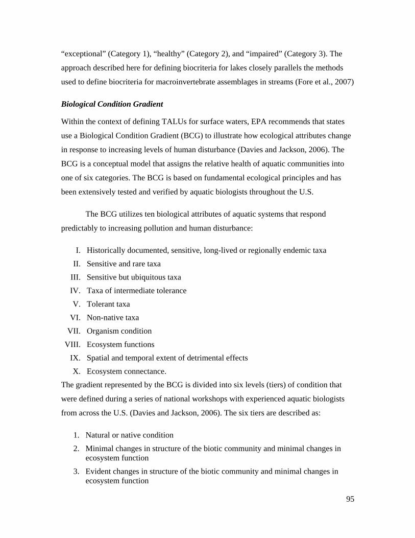
95

“exceptional” (Category 1), “healthy” (Category 2), and “impaired” (Category 3). The

approach described here for defining biocriteria for lakes closely parallels the methods

used to define biocriteria for macroinvertebrate assemblages in streams (Fore et al., 2007)

Biological Condition Gradient

Within the context of defining TALUs for surface waters, EPA recommends that states

use a Biological Condition Gradient (BCG) to illustrate how ecological attributes change

in response to increasing levels of human disturbance (Davies and Jackson, 2006). The

BCG is a conceptual model that assigns the relative health of aquatic communities into

one of six categories. The BCG is based on fundamental ecological principles and has

been extensively tested and verified by aquatic biologists throughout the U.S.

The BCG utilizes ten biological attributes of aquatic systems that respond

predictably to increasing pollution and human disturbance:

I. Historically documented, sensitive, long-lived or regionally endemic taxa

II. Sensitive and rare taxa

III. Sensitive but ubiquitous taxa

IV. Taxa of intermediate tolerance

V. Tolerant taxa

VI. Non-native taxa

VII. Organism condition

VIII. Ecosystem functions

IX. Spatial and temporal extent of detrimental effects

X. Ecosystem connectance.

The gradient represented by the BCG is divided into six levels (tiers) of condition that

were defined during a series of national workshops with experienced aquatic biologists

from across the U.S. (Davies and Jackson, 2006). The six tiers are described as:

1. Natural or native condition

2. Minimal changes in structure of the biotic community and minimal changes in ecosystem function

3. Evident changes in structure of the biotic community and minimal changes in ecosystem function

96

4. Moderate changes in structure of the biotic community with minimal changes in ecosystem function

5. Major changes in structure of the biotic community and moderate changes in ecosystem function

6. Severe changes in structure of the biotic community and major loss of ecosystem function.

Davies and Jackson (2006) recommend that regional biological experts adapt the

conceptual tiers described by the BCG to local conditions using data from a regional

monitoring program. This was the approach adopted by Florida DEP to define biocriteria

for the LVI.

Methods

A panel of 20 experienced plant ecologists, all with more than five years of experience,

was convened as part of a workshop to develop a BCG for Florida lakes (App. Table 7.1).

Participants were asked to apply and calibrate the general BCG model to macrophyte data

collected from Florida lakes. Results from the workshop were used to define biological

thresholds (biocriteria) for the LVI.

Prior to the workshop, experts were provided with background literature on the

BCG concept (Davies and Jackson, 2006; Stoddard et al., 2006) and a description from

DEP of the workshop process and the LVI sampling method. Experts were informed that

they would be asked during the workshop to review macrophyte data from individual

lakes and assign each sample a score from 1 (best) to 6 (worst), signifying their

assessment of the biological condition represented by the plant assemblage.

The experts were given taxa lists and metric values for each lake. Data were

provided for 15 lakes in the north and 15 in the south; experts were told whether lakes

were located in the north or south. Experts were not given LVI index values or any

physical, chemical, or habitat descriptions of the sites.

Lake visits were selected primarily from the 2005-2006 data, with additional lake

visits from the southern region as needed. Within each region, the samples with LVI

scores closest to the 10th, 20th, 30th, 40th, 50th, 60th, 70th, 80th, and 90th percentiles of LVI

97

scores for that region were chosen (nine visits; “LVI %iles” in App. Table 7.2). Then one

lake visit was randomly selected from each of HDG levels 1-6 for each region (six visits;

“HDG cat” in App. Table 7.2).

During the workshop, experts were given the opportunity to discuss their rationale

for scoring a lake, and, if they desired, to change their score for a lake based on their

assessment from the discussions (Delphi method). Scoring sheets were provided to each

expert for recording both initial and final BCG scores. Experts were requested to indicate

what relevance they ascribed to their BCG scores. More specifically, they were asked to

record the maximum BCG score that they believed did not meet the interim goals of the

Clean Water Act (impaired site; does not meet designated use). In other words, lakes

below a selected tier score would be considered “impaired.” Experts were also asked to

record the minimum score they believed represented an exceptional condition.

Before the TALU guidance was developed, many states used an approach based

on reference site condition to develop biocriteria (EPA, 2006). Typically percentiles of

index values for references sites are used to define thresholds. A buffer derived from the

variability of reference site index values may also be used to define the lowest index

value that indicates departure from reference condition, or impairment. Although not

used to define thresholds for the LVI, LVI statistics for reference lakes are reported here

because this method has been widely used before the more recent recommendations from

EPA to use the BCG approach.

98

App. Table 7.1. Workshop participants, their affiliation and years of experience working with plants. Three participants had <5 years of experience and their scores were not included in threshold calculations.

Expert Affiliation Years of Experience

Loran Anderson FSU Emeritus >60

Erica Anderson DEP - Bureau Aquatic Plant Management >5

David Hall Independent consultant 47

Jess Van Dyke DEP - Bureau Aquatic Plant Management 37

Joe Hinkle DEP - Bureau Aquatic Plant Management 33

Jeff Schardt DEP - Bureau Aquatic Plant Management 31

John Rodgers DEP - Tampa 30

Jackie Smith DEP - Bureau Aquatic Plant Management 25

Robbie Lovesrand DEP - Floral City 20

Ed Harris DEP - Orlando 20

Katherine Gilbert DEP - Tallahassee 20

John Tobe ERC, Inc 20

Terry Sullivan DEP - Floral City 20

Jeff Holland Reedy Creek Improvement District 17

David Demmi DEP - Bureau Aquatic Plant Management 15

Christine Keenan DEP - Tallahassee 15

Nathalie Visscher DEP - Orlando 8

Peggy Morgan DEP - Tampa 5

Julie Espy City of Tallahassee 5

Dana Denson DEP - Orlando 5

Kelli Gladding DEP - Orlando 4

Danielle Sobczak DEP - Bartow 2

Marissa Rodriguez DEP - Orlando 1.5

99

App. Table 7.2. Lake visits used in the BCG workshop. Shown are station nickname, STORET number, macrophyte ID, date of sampling, LVI, HDG, LDI and the method used to select the lake.

BCG ID Station Nickname STORET

MacroID Date LVI HDG LDI

Selection method

N01 LKTHOMAS 24040132 3861 10/27/2005 48 2 3.8 LVI %iles

N02 PETTYGULF 22020129 4867 10/20/2005 33 4 4.4 HDG cat

N03 CHERYNEUNK 21010039 5123 10/13/2005 69 3 5.9 HDG cat

N04 PALSTCTREF 19010044 5201 10/11/2005 94 1 1.0 HDG cat

N05 ORANG161 26010887 5282 11/2/2005 41 5 6.4 LVI %iles

N06 LKSAUNDERS 20020166 5341 10/27/2005 63 5 4.6 HDG cat

N07 MARINERLK 20020165 5361 10/25/2005 82 2 3.8 HDG cat

N08 RSNAKEREF 32030099 5381 11/10/2005 82 0 1.7 LVI %iles

N09 LKSTANLEY 33040029 5383 10/26/2005 85 3 7.1 LVI %iles

N10 NW3SL2065 29664 6061 7/26/2006 78 2 2.6 LVI %iles

N11 LKSTANLEY 33040029 6241 11/6/2006 68 3 7.1 LVI %iles

N12 HIAWATHA 22020042 6364 10/19/2006 85 1 2.2 LVI %iles

N13 LONG POND 32020131 6409 10/16/2006 60 3 2.7 LVI %iles

N14 LKFRANCES 21020123 6410 11/15/2006 68 6 7.0 HDG cat

N15 BAKER15 21010011 6419 11/1/2006 87 1 2.0 LVI %iles

S01 LKYELHAM 25010080FTM 502 8/13/2002 38 3 1.9 HDG cat

S02 LKPLACIDNO 26010650FTM 546 8/20/2002 54 3 3.8 LVI %iles

S03 LKVERONMID 26010339FTM 921 10/27/2003 36 4 6.6 LVI %iles

S04 CYPRESSLK1 26010075 5621 5/10/2006 41 0 1.8 LVI %iles

S05 SAR616NL SAR616NL 6322 11/1/2006 63 2 1.1 HDG cat

S06 LKHUNTER 24030148 6323 10/19/2006 63 5 6.8 HDG cat

S07 HIL540NL HIL540NL 6324 9/28/2006 49 1.5 1.9 LVI %iles

S08 SW3SL2006 30724 6367 8/8/2006 22 4 4.2 HDG cat

S09 GENTNEREF 26010988 6373 10/16/2006 66 1 1.9 HDG cat

S10 SW3SL2013 30726 6376 9/5/2006 18 6 7.3 HDG cat

S11 SW3SL2082 30736 6392 8/22/2006 31 4 5.5 LVI %iles

S12 SW3SL2114 30745 6400 8/15/2006 72 4.5 3.3 LVI %iles

S13 SW3SL2170 30748 6401 9/6/2006 12 6 8.2 LVI %iles

S14 SW3SL2102 30741 6403 8/24/2006 41 5 7.7 LVI %iles

S15 LKEDEN 28010595 6426 11/8/2006 42 2 1.0 LVI %iles

100

Results

Each expert assigned a BCG to all of the 30 lakes (App. Table 7.3). After reviewing the

data, most experts selected tiers 1 and 2 as exceptional aquatic life use (16 out of 19; 1

with no response; App. Table 7.4). Most experts agreed that tiers 5 and 6 indicated

impairment or failure to support aquatic life use (13 out of 20). Seven experts thought the

line for impairment should be higher: two identified tier 3 and five identified tier 4 as

failing to support aquatic life use.

BCG scores from the experts were averaged to define thresholds for LVI. For the

definition of the impairment line, an average of 4.6 was calculated from the experts’

definitions. We rounded this value to the nearest half category (4.5) because BCG scores

were not considered in increments of 0.1, and a value of 4.6 implied an accuracy that was

not supported by the discussion. For the definition of the exceptional category, a value of

2.0 was calculated from the experts definitions. To translate these thresholds into LVI

values, a regression equation was used (App. Figure 7.1).

A BCG score of 4.5 corresponded to an LVI value of 37 as the impairment

threshold. Thus, based on the recommendations of 20 regional experts, LVI values from

0-37 are proposed as Category 3 (provisionally interpreted as “impaired”). A BCG score

of 2.0 corresponded to an LVI value of 78 as the threshold between Categories 2 and 1

(provisionally interpreted as “healthy” and “exceptional”).

101

App. Table 7.3. Lake visit, BCG scores for each expert, median BCG for each lake, and LVI.

Lake E01 E02 E03 E04 E05 E06 E07 E09 E10 E12 E13 E14 E15 E17 E18 E19 E20 E21 E22 E23 MeanBCG

MedianBCG

LVI

N01 4 4 4 4 5 5 4 3 5 3 4 5 5 4 4 4 5 4 4 4 4.2 4 48N02 3 5 6 5 6 5 5 5 5 5 5 5 6 5 5 5 5 5 5 5 5.1 5 33N03 4 3 3 3 3 3 3 3 4 3 3 4 4 3 3 3 4 1 3 3 3.2 3 69N04 1 1 1 1 1 2 1 1 1 2 1 4 2 2 2 1 2 2 2 2 1.6 2 94N05 5 5 5 4 4 4 4 3 4 4 4 2 4 3 3 4 4 3 3 3 3.8 4 41N06 3 3 4 3 4 4 4 3 3 3 4 3 4 3 3 3 3 4 3 3.4 3 63N07 2 1 1 1 1 2 1 1 1 1 1 3 1 1 2 1 4 2 1 1 1.5 1 82N08 2 1 1 3 1 1 1 1 1 1 1 2 1 1 1 1 1 2 1 1 1.3 1 82N09 2 2 1 2 2 2 2 1 2 2 2 2 2 2 2 2 1 2 2 2 1.9 2 85N10 3 2 2 2 2 3 2 2 2 3 2 2 3 2 3 2 3 2 2 3 2.4 2 78N11 3 2 1 2 2 2 2 2 2 2 2 2 2 2 3 2 3 2 2 2 2.1 2 68N12 1 1 1 1 1 2 1 1 1 1 1 1 1 1 1 1 3 1 1 1 1.2 1 85N13 2 3 2 3 2 3 3 4 3 3 3 3 3 2 3 3 1 3 3 3 2.8 3 60N14 3 4 3 4 3 4 4 3 4 3 3 3 4 3 4 3 3 4 3 3 3.4 3 68N15 1 1 1 1 1 1 1 1 1 1 1 1 1 1 2 1 4 2 1 1 1.3 1 87S01 5 5 5 5 5 5 5 4 5 5 5 4 5 5 5 4 2 5 4 5 4.7 5 38S02 3 3 3 4 3 3 3 4 3 3 4 3 3 4 4 3 5 3 4 3 3.4 3 54S03 5 5 4 5 5 5 5 5 5 5 5 4 4 5 5 5 4 4 4 5 4.7 5 36S04 4 3 4 4 4 4 4 5 5 5 4 5 5 4 4 5 5 2 4 4 4.2 4 41S05 3 3 3 2 2 3 3 2 2 2 3 2 2 2 2 3 5 2 2 2 2.5 2 63S06 3 3 3 4 2 4 4 3 3 3 4 3 3 3 3 3 2 3 2 3 3.1 3 63S07 4 3 4 4 4 4 4 5 4 5 4 4 6 5 4 5 3 3 5 4 4.2 4 49S08 5 5 5 5 5 5 5 4 5 4 5 5 4 5 5 5 5 5 5 4 4.8 5 22S09 3 2 3 2 3 2 3 4 3 3 3 2 3 3 3 3 5 2 3 3 2.9 3 66S10 5 6 6 5 5 5 5 3 6 5 5 5 5 4 5 5 5 5 4 4 4.9 5 18S11 5 5 6 4 5 5 5 5 4 4 5 5 5 5 5 5 4 4 4 4 4.7 5 31S12 4 3 3 3 3 3 4 3 3 4 3 3 4 4 3 3 3 4 2 3 3.3 3 72S13 5 6 6 5 5 5 5 6 5 6 5 6 6 6 6 5 5 5 5 6 5.5 5 12S14 4 4 4 4 4 4 4 5 4 4 4 4 4 4 4 4 5 4 4 4 4.1 4 41S15 3 4 4 3 4 3 4 4 4 4 3 3 3 4 4 3 5 4 5 3 3.7 4 42

App. Table 7.4: Experts’ selection of threshold values of BCG that indicate exceptional condition and impaired condition.

Expert Exceptional Impaired/ Does Not Meet

E01 1 5 E02 2 5 E03 2 5 E04 1 4 E05 2 5 E06 1 4 E07 2 5 E09 2 5 E10 3 5 E12 2 3 E13 2 3 E14 3 6 E15 2 4 E17 ND 5 E18 2 4 E19 2 5 E20 2 5 E21 2 4 E22 2 5 E23 3 5

MEDIAN = 2 5 AVERAGE = 2 4.6

103

0.5 1.0 1.5 2.0 2.5 3.0 3.5 4.0 4.5 5.0 5.5 6.0Expert's Biological Condition Gradient score (mean)

0

10

20

30

40

50

60

70

80

90

100LV

I

App. Figure 7.1. LVI values were highly correlated with the BCG scores assigned by the experts (Pearson’s r = 0.89). Shown are the regression line (solid black) and threshold values for impaired lakes (LVI = 37; red dashed lines) and exceptional lakes (LVI=78; green solid line).

Reference sites

Initially, 37 reference lakes with HDG = 0 were identified from the 2005–2006 validation data

set. Recall that HDG = 0 does not mean no human disturbance, but minimal human disturbance.

This initial list of lakes was evaluated by biologists who had sampled the lakes and were familiar

with local conditions. If any lake could not be confidently labeled as "minimally disturbed," it

was excluded from the reference set based on the best professional judgment of the biologist.

This process yielded a total of 22 reference lakes for calculating statistics for the LVI (App.

Table 7.5). Notably, only two reference lakes could be identified for the southern section of the

state.

Paralleling an approach used by other states, a buffer of LVI values below the 10th

percentile was used to represent the natural variability associated with field sampling that could

be due to water level fluctuation, weather, or time of sampling. Half the 90% confidence interval

104

(12.0) was subtracted from the 10th percentile of LVI as: 66–12.0 = 54 (App. Table 7.6;

Appendix 6). Values below 54 would be considered impaired using this approach. This value

(LVI = 54) for the impairment line is 17 points higher than the threshold derived from the BCG

approach (LVI = 37).

In contrast, the higher threshold for the LVI value (dividing “exceptional” from “healthy”

lakes) based on the reference site approach was very close to the value from the BCG workshop.

Subtracting half the 90% confidence interval from the 90th percentile for LVI as: 92–12.0 = 80,

yielded a value only 2 points higher than the LVI threshold derived from the BCG workshop.

App. Table 7.5. Reference lake STORET, nickname, region, date of sampling LVI, and LDI.

STORET Station Nickname Region Date LVI LDI

26010301 NONAREF North 11/1/2005 93 1.6 27144 SJ6SL2036 North 9/16/2005 92 1.0 29671 NW3SL2086 North 8/1/2006 92 1.1 27141 SJ6SL2020 North 9/2/2005 92 1.0 27150 SJ6SL2052 North 9/2/2005 91 1.1

32020104 CASSCTREF North 11/1/2006 89 1.0 32010045 DUNFORDREF North 10/12/2005 86 1.0 26010300 MUDTST North 12/7/2005 85 1.2

26762 NW2SL2126 North 8/4/2005 84 1.8 14441 NWC-LL1002 North 10/26/2005 83 1.6

20020496 SELLCTREF North 10/18/2006 82 1.8 26742 NW2SL2025 North 7/7/2005 79 1.4

32030097 PORTERREF North 11/1/2005 78 1.5 26010310 ANNMIDREF South 11/3/2005 78 1.7

26753 NW2SL2086 North 7/28/2005 75 1.6 27166 SJ6SL2098 North 9/1/2005 74 1.7

20010080 BUCKLKONF North 6/1/2005 73 2.0 32030099 RSNAKEREF North 10/31/2006 70 1.7

26769 NW2SL2158 North 7/27/2005 67 1.6 26010988 GENTNEREF South 10/16/2006 66 1.9

22100 NW1-LL2007 North 11/2/2006 60 1.4 29655 NW3SL2045 North 7/11/2006 43 1.3

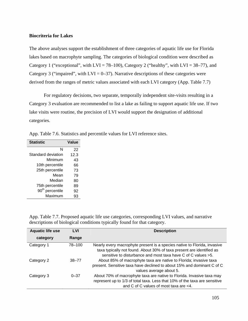
105

Biocriteria for Lakes

The above analyses support the establishment of three categories of aquatic life use for Florida

lakes based on macrophyte sampling. The categories of biological condition were described as

Category 1 (“exceptional”, with LVI = 78–100), Category 2 (“healthy”, with LVI = 38–77), and

Category 3 (“impaired”, with LVI = 0–37). Narrative descriptions of these categories were

derived from the ranges of metric values associated with each LVI category (App. Table 7.7)

For regulatory decisions, two separate, temporally independent site-visits resulting in a

Category 3 evaluation are recommended to list a lake as failing to support aquatic life use. If two

lake visits were routine, the precision of LVI would support the designation of additional

categories.

App. Table 7.6. Statistics and percentile values for LVI reference sites.

Statistic Value

N 22 Standard deviation 12.3

Minimum 43 10th percentile 66 25th percentile 73

Mean 79 Median 80

75th percentile 89 90th percentile 92

Maximum 93

App. Table 7.7. Proposed aquatic life use categories, corresponding LVI values, and narrative descriptions of biological conditions typically found for that category.

Aquatic life use category

LVI Range

Description

Category 1 78–100 Nearly every macrophyte present is a species native to Florida, invasive taxa typically not found. About 30% of taxa present are identified as

sensitive to disturbance and most taxa have C of C values >5. Category 2 38–77 About 85% of macrophyte taxa are native to Florida; invasive taxa

present. Sensitive taxa have declined to about 15% and dominant C of C values average about 5.

Category 3 0–37 About 70% of macrophyte taxa are native to Florida. Invasive taxa may represent up to 1/3 of total taxa. Less that 10% of the taxa are sensitive

and C of C values of most taxa are <4.

106

References

Davies, S.P. and S.K. Jackson. 2006. The biological condition gradient: a descriptive model for interpreting change in aquatic systems. Ecological Applications 16(4):1251-1266.

Fore, L. S., R. Frydenborg, D. Miller, T. Frick, D. Whiting, J. Espy, and L. Wolfe. 2007. Development and Testing of Biomonitoring Tools for Macroinvertebrates in Florida Streams (Stream Condition Index and Biorecon). Final Report to FDEP. Available: ftp://ftp.dep.state.fl.us/pub/labs/assessment/sopdoc/sci_final.pdf.

National Research Council (NRC). 2001. Assessing the TMDL approach to water quality management. Water Science and Technology Board, Division on Earth and Life Studies. National Academy Press, Washington, DC.

Stoddard, J.L., D.P. Larsen, C.P. Hawkins, R.K. Johnson, and R.H. Norris. 2006. Setting expectations for the ecological condition of streams: the concept of reference condition. Ecological Applications 16(4):1267-1276.

U.S. Environmental Protection Agency (EPA). 2005. Draft. Use of biological information to better define designated aquatic life uses in state and tribal water quality standards: tiered aquatic life uses. Washington, D. C.: Office of Science and Technology.

———. 2006. Best Practices for Identifying Reference Condition in Mid-Atlantic Streams. Washington, D. C.: Office of Environmental Information. EPA-260-F-06-002. Available: http://www.epa.gov/bioindicators/html/publications.html.