Embed Size (px)
Citation preview

§Bechtel Nuclear, Security & Environmental Inc. includes the former Bechtel Systems & Infrastructure Inc. and Bechtel Power Corporation starting
January 01, 2015
ASSESSMENT OF COOLING TOWER DISCHARGE RECIRCULATION AND
DISPERSION USING CFD TECHNIQUES
S. Pal Bechtel Nuclear, Security & Environmental Inc. §
Reston, VA
L. J. Peltier Bechtel Nuclear, Security & Environmental Inc. §
Reston, VA
A. Rizhakov Bechtel Nuclear, Security &
Environmental Inc. § Reston, VA
M. P. Kinzel Pennsylvania State University
State College, PA
M. H. Elbert Bechtel Nuclear, Security &
Environmental Inc. § Reston, VA
Kelly J Knight
Bechtel Nuclear, Security & Environmental Inc. § Reston, VA
S. Rao Bechtel Nuclear, Security & Environmental Inc. §
Reston, VA
1. ABSTRACT
The performance of cooling towers, whether operating by themselves, or in close vicinity of other cooling towers can be adversely affected by the re-ingestion of the cooling tower discharge into the tower intakes. The recirculation of the discharge from a wet cooling tower raises the wet bulb temperature of the air entering a wet cooling tower. Current design strategies, often account for this discharge re-ingestion issue, through a conservative adjustment to the far field ambient wet bulb temperature to calculate the actual intake wet bulb temperature. Critical applications, such as those related to nuclear safety applications where there is concern about cooling tower performance, may require more accurate and comprehensive assessment of the recirculation and dispersion of cooling tower discharge. Gaussian plume models alone are of limited use when dealing with discharges in the vicinity of large structures. This paper discusses the use of a computational fluid dynamics approach to evaluate worst case discharge recirculation effects in cooling towers. The bounding design values of tower intake wet bulb temperature increase due to recirculation (ingestion of tower’s own discharge), and interference (ingestion of another interfering tower’s discharge), are calculated considering the various conditions of cooling tower operation, ambient temperature, humidity and wind conditions. The RANS CFD model used in the study is evaluated against published experimental data for flow over bluff bodies at high Reynolds numbers, and experimental data on buoyant jets in cross flow.
2. INTRODUCTION
This paper presents a summary of the Ultimate Heat Sink (UHS) cooling tower interference and recirculation assessment performed for a proposed Nuclear Power Plant (NPP). The proposed UHS has four mechanical, induced draft, wet cooling towers as shown in figure 1. Each tower has two identical fans in two cells which share a common basin. The proposed design is expected to handle a Design Basis Accident (DBA) with two cooling towers in operation, that will be always available considering one down for single failure, and one down for maintenance. The following sections discuss the decoupled analysis approach, the computational fluid dynamics (CFD) code validation, and the CFD model results.
3. METHODOLOGY
3.1. UHS Design and Sizing With Assumed Intake Wet Bulb Increase
Typically only estimates of interference and recirculation effects are available for a proposed NPP design. Initial UHS design and sizing is performed with assumed recirculation and interference corrections. Computer programs like PDAP and UHSSIM can calculate UHS performance characteristics and response to a specific accident scenario (Ref. 1, 2). It should be confirmed that cooling tower basin water temperature remains below the recommended level in any accident scenario. A subsequent confirmatory study, similar to the one presented in this paper, is necessary to confirm the bounding recirculation and interference values assumed in design calculations.
Proceedings of the ASME 2015 Power Conference POWER2015
June 28-July 2, 2015, San Diego, California
POWER2015-49033
1 Copyright © 2015 by ASME

Fig. towerview)
Fig. 2coolin
3.2. CR
P
Fbuoyapositivaporspeedmakecondidepenthe rintakewith descrfound
1. Schematic rs and nearby).
2. Typical secng tower. Arrow
CFD AssessmeRecirculation
Problem Physic
For mechanicaant jet becauseive buoyancy r mass fractiond conditions, te interference itions can leadnding on buildrelative locatioes. A general a wind velocit
ribing the behad in Ref. 4. Th
F
showing relatiy structures ar
ction view shows show the di
nts of Cooling
cs
al draft cooline of the momenis attributed t
n and fluid temthe fan discha
and recircul to significant
ding layout, wion of the ope
model of a sty field can be avior of buoya
he external win
Fan discharge
ive location oround the con
owing arrangemirection of air f
Tower Interfer
ng towers the ntum imparted to higher than
mperature. In caarge is lofted hlation negligibrecirculation and speed, wind
erating tower single buoyant
found in Ref.ant jets in crond flow pattern
Induced d
Spray hea
Fill media
Basin
Ambien
of UHS coolinntainment (pla
ment inside thflow.
rence and
discharge is by the fan. Th
n ambient watealm or low winhigh enough tble. The winand interferencd direction, andischarges an
t jet interactin 3. Correlation
oss flow can bn is modified b
draft fan
ader
a
nt air intake
ng an
he
a he er nd to nd ce nd nd ng ns be by
the prnumbeand opreleva
i.iiiiiivv.
F
Tby reevapoThe bon mainto tcondit
Fstudy,the dConsidspeedsinterfeand laare ins
BNPP strivialtempeconstatowerall opdischainteracrecircuessent
i.iiiii
iv
Tabl
resence of buer based on buperating scena
ant to the problFan dischar
. Fan dischari. Fan dischar
v. Reynolds n. Ambient str
Factors Affectin
The UHS abilitecirculation anoration potentiaounding interfaximum instanthe atmosphertions, and assuor the mechan, ~ 10
discharge is edering the buis which mayerence, it is exarge scale turbsensitive to
Based on analysite, ambient l wind speederature and loant speed fan
produces apperating conditiarge looses itsction of the fanulation and intially determine
Wind direc. Nominal wi. Operating s
intakes in thscenarios ar
v. Discharge F
le 1: Different out of
Operatin
uildings and isuilding dimensiario, the relevalem of UHS disrge Reynolds nrge Froude numrge speed to wi
number for flowratification par
ng Interference
ty to reject hend interferencal, and high amference and recntaneous accidre, with speciuming a steady ical draft cooli. The evolutio
essentially indilding dimensioy lead to si
xpected that bulence feature
for these Reysis of meteoro
stratification cds coexist wiow evaporatiused in the p
proximately theions. The locas jet charactern discharge witnterference foed by:
ction wind speed
scenario – layhe operating tore shown in tabFroude number
UHS operatinf the four towe
ng Scenario A B C D E F
s characterizedions. For givenant non-dimenscharge dispersnumber, mber, ind speed ratio
w over buildingrameter,
e and Recircula
at is most advce under condmbient wet bulbcirculation is cdent heat load fied ambient basin tempera
ing towers inveon of the jet chdependent of ons, and the nignificant rec
10 .es for flow oveeynolds numberological data focan be neglecth high ambon potential proposed NPPe same discha
ation where theristics is deteth the external
or a UHS co
yout of active owers. The diffble 1. r,
g scenarios coners in operation
Operating TowTowers 1 & Towers 3 & Towers 1 & Towers 1 & Towers 2 & Towers 2 &
d by Reynoldn wind directionsional numbersion are:
o, gs,
ation
versely affecteditions of lowb temperaturesalculated basebeing releasedhigh humidity
ature. estigated in thiharacteristics o
(Ref. 3)non-trivial windcirculation anThe mean flower the buildingrs (Ref. 5). or the proposeted when nonient wet bulbconditions. A
P UHS coolingarge velocity ine cooling toweermined by th
wind. Thus tholing tower i
discharges anferent operating
nsidering two n.
wers 2 4 3 4 3 4
ds n rs
d w s. d d y
is of ). d d w gs
d n-b A g n
er e e is
d g
2 Copyright © 2015 by ASME

Inputs for Calculating Bounding Intake Wet Bulb Increase
To calculate the bounding recirculation and interference the following inputs are used to calculate the highest intake wet bulb increase:
i. Heat load – bounding value based on peak accident heat release
ii. Discharge relative humidity and dry bulb temperature – bounding value calculated based on pure-water vapor pressure and lowest possible dry bulb temperature increase over the ambient value for the specified heat load. This is ensured by forcing 100% relative humidity at the fan discharge for the conditions analyzed. This approach minimizes the plume buoyancy for a given heat load.
iii. Wind speed(s) – selected speeds based on site specific meteorological data and results from a passive scalar dispersion study
iv. Wind direction(s) – selected wind directions for specific operating scenarios based on results from the passive scalar dispersion study
4. CFD MODEL DETAILS
4.1. CFD Model Domain
The computational model extends from the ground to 600m height and extends over all significant structures in the vicinity of the cooling towers shown in figure 1. The CFD model is 1700m x 1700m in plan view and the terrain is assumed flat except the modeled structures. The modeled structures are confined within a 650m diameter circle and include the cooling towers, and other buildings that are expected to affect the local air flow and dispersion of cooling tower discharge.
As shown in figure 2, the air enters the cooling tower through two rectangular openings on both sides of the tower. The CFD model does not include the details of the flow inside the cooling tower. The flow (entering the cooling tower) leaves the CFD model at the intake openings of the cooling tower. The flow (discharged from the cooling tower) enters the CFD model from the fan discharge openings at the top of the cooling tower. The exact flow conditions at fan discharge are calculated separately outside the CFD model.
4.2. Governing Equations
The governing equations solved for the plume dispersion CFD model are conservation equations for mass, momentum, energy and species. The flow is modeled as multi-component mix of air and water vapor. The flow is a low speed compressible flow. To handle the adiabatic lapse rate, and the associated density and pressure profiles using an incompressible flow formulation, a virtual potential temperature approach is used (Ref. 6). The mathematical formulation is summarized in equations 1 through 8.
The potential temperature ( ) is the temperature of a parcel of moist air adiabatically compressed to the reference
pressure at grade. The virtual potential temperature ( v ) is the
temperature of dry air at reference pressure having the same energy content as the parcel of moist air compressed adiabatically to the reference pressure at grade. The energy
equation is formulated in terms of v . If the water vapor mass
fraction is constant with elevation, the virtual potential temperature does not change with elevation in a neutrally stable atmosphere. The different temperature profiles are shown in figure 3.
q
Cp
R
P
PT
23.010
(1)
)61.01( qv (2)
Fig. 3. Physical temperature, potential temperature, and virtual potential temperature profiles in a neutrally stable atmosphere with constant water vapor mass fraction.
Buoyancy effects are accounted for using a Boussinesq approximation with a constant thermal expansion coefficient, .
rvv
0
0 (3)
where,
rv
1 (4)
The governing equation for the mean velocity is the incompressible Reynolds-Averaged Navier-Stokes equation.
30
0
1ir
v
rvv
j
iT
jiji
j
i gx
U
xx
PUU
xt
U
(5)
The governing equation for mass conservation is
0
i
i
x
U (6)
The governing equation for energy conservation is the Reynolds-Averaged advection/diffusion equation written in terms of virtual potential temperature.
0
100
200
300
400
500
600
304 306 308 310 312 314 316
Elevation above grade (m
)
Temperatures in Kelvin
Physical Temperature (K) Potential Temperature (K)
Virtual Potential Temperature (K)
3 Copyright © 2015 by ASME

j
vTT
jvj
j
v
xxU
xt
1Pr (7)
where, is the thermal diffusivity, and PrT is the turbulent Prandtl number which is a turbulence model parameter. The governing equation for moisture conservation is the Reynolds-Averaged scalar advection/diffusion equation:
jTT
jj
j x
qSc
xqU
xt
q 1 (8)
is the water vapor diffusivity in air, and ScT is the turbulent
Schmidt number which is a turbulence model parameter. A turbulence model is used to calculate the turbulent
momentum diffusivity T . The turbulence model equations
should incorporate appropriate modifications for buoyancy.
4.3. CFD Model Verification and Validation
The verification and validation of the buoyant plume CFD model used to calculate the actual wet bulb temperature increase at the tower intakes is described in Annexure A. Annexure B describes the verification and validation of the CFD model used in passive scalar study to identify the operating scenarios and wind directions of concern. The buoyant plume model post-processing provides the expected increase in the intake wet-bulb temperature considering effects of plume buoyancy. In contrast, the passive scalar model identifies the expected high recirculation and interference cases by comparing passive scalar ingestion levels.
4.4. Buoyant Plume CFD Model Mesh and Boundary Conditions
The mesh of the computational domain is comprised of polyhedral cells in the interior. Prism layers are provided on the walls and the ground to resolve the boundary layer. The boundary conditions on the model are summarized below:
i. Ground – no-slip impermeable with zero gradients for virtual potential temperature and water vapor mass fraction.
ii. Top of the domain – symmetry conditions i.e., zero gradient normal to the boundary for all variables
iii. Far field wind conditions – (a) prescribed velocity, density (constant), turbulent kinetic energy, turbulence dissipation, water vapor mass fraction (constant), and virtual potential temperature (constant) profiles as function of height on inlet boundaries where far field flow enters the domain. The incoming velocity and turbulence profiles are calculated for the specific turbulence model being used by simulating an equilibrium boundary layer over a flat plate. This is done by imposing a specified pressure gradient between periodic inlet and outlet boundaries. The pressure gradient is adjusted to match the desired nominal velocity at the reference elevation. The calculated velocity profile for 5 m/s nominal wind speed is compared to the log law profile in figure 4.
The turbulence quantity profiles from the periodic flat plate boundary layer model are similarly used as a boundary conditions at the far field inflow locations. (b) Prescribed pressure (hydrostatic) is applied at outflow boundaries where the external flow is expected to leave the domain.
iv. Cooling tower fan discharges for towers in operation – these are inlet boundaries in the CFD model where a uniform plug velocity profile with specified turbulence intensity and length scale is applied. Calculated values of water vapor mass fraction and virtual potential temperature are applied at the fan discharges. For the 5 m/s nominal wind speed the ratio of the fan discharge speed to the free stream wind speed at 60m elevation is approximately 1.246 in the buoyant plume CFD model. It decreases as the nominal wind speed is increased. The fan discharges at the non-operating towers are modeled as impermeable walls.
v. Cooling tower intake openings for towers in operation – these are reverse inlets with outgoing uniform plug velocity profiles corresponding to calculated mass inflows into the tower intakes. The intakes on the non-operating towers are modeled as impermeable walls.
Fig. 4. Far field velocity profile calculated using CFD model of an equilibrium boundary layer compared to a standard logarithmic profile with appropriate roughness parameter.
4.5. Calculation of CFD Model Boundary Conditions at Cooling Tower Fan Discharges
The calculation of the tower discharge conditions is done using the peak accident heat load, specified far field ambient dry and wet bulb temperatures, and assuming steady state in the basin. The cooling tower intake temperature and water vapor mass fraction are taken from the buoyant plume CFD model. These inputs are summarized in table 2. The discharge condition calculation illustrated in figure 5 enforces the mass, momentum, energy, and species balance subject to the specified relative humidity constraint at the cooling tower discharge.
0
20
40
60
80
100
120
140
160
180
200
0 1 2 3 4 5 6 7
Elevation (m)
Velocity (m/s)
Velocity[i] Velocity‐loglaw (m/s)
Conditions chosen to match field data at 60m
4 Copyright © 2015 by ASME

Thermpsych
Dperfoexact 13). Tat theand mseparbut, aplume
TConsiand isaturawet chumidtowercondemixinhumidcalcutempedoes latent
Ldischwith humidtemperelativthe dambiespecifgivenconst
Table
InpAmAmHea
Tow(coBasTowtemvap
modynamic anhrometric data Design calcularmance using
t discharge dryThe calculatione tower dischamass transfer rate heat and ma conservativee is used to ass
The basin wateidering dissolvincreases the ated to slightlycooling tower dity and high r discharge enses and releng with the amdity as the m
ulation. The sinerature formulnot model dro
t heat in the enLower relativeharge is observ
low heat loaddity at discherature that is ve humidity atdischarge dry ent dry bulb. Tfication is the
n fan flow and traint is lowere
e 2: Ambient a
put mbient wet bulbmbient dry bulbat load
wer fan floonstant) sin Temperaturwer intake
mperature andpor mass fractio
nd transport prois taken from R
ations for towMerkel’s me
y bulb temperatn of the exact darge will requi
calculation (Rmass transfer e calculation osess bounding rer properties areved solids redu
discharge dryy supersaturatedischarge forheat loads. F
is supersatureases latent he
mbient. This jusmaximum humi
ngle phase, inclation using thoplet dispersioergy equation
e humidity (< ved only for dds. If, the calharge produclower than thet the discharge
bulb temperaThe CFD modee Froude numheat load incrd.
and tower intakand fan flo
Valb 85.b 99.
Peavar(De
ow rate 1,1(54
re Stestatic
d water on
(a) or (b) mixat g
operties of air Ref. 7 through
wers generally ethod without ture and humiddry bulb and reire detailed anRef. 14-15). Icalculation is
of the buoyancrecirculation ane taken as thosuces the watery bulb tempeed condition ir conditions oFor cases, whrated, excess eat once the dtifies the use oidity for the tcompressible vhe Boussinesqon, and does nformulation. 100%) at wet
dry and hot colculation with ces a dischae ambient value is lowered frature becomesel input most im
mber, The Froureases as the re
ke conditions, tow rate.
lue 3 °F 0 °F
ak heat loadrying heat loesign Basis Ac49,000 acfm
42.27 m3/s per feady
From CFD mo
Prescribed volxture of far fielgrade and towe
and water, an12. predict overapredicting th
dity (Ref. 1 anelative humiditnd separate heaIn this study, not carried ou
cy of the towend interferencese of pure water vapor pressurerature. A neas expected at
of high ambienere the coolin
water vapodischarge start
of 100% relativtower dischargvirtual potentia
q approximationot consider th
t cooling toweonditions and/o
100% relativarge dry bulue, the specifierom 100% unts the same ampacted by thude number foelative humidit
tower heat load
d from time oad in DBAcident)
m per fan fan)
odel
lumetric ratio ld ambient air er discharge
nd
all he nd ty at a
ut er e. er. re ar a
nt ng or ts
ve ge al
on he
er or ve lb ed til as is or ty
d,
Fig. conserat gradtower liquid
4.6. Cth
Tanalysplumeconditinflowused tof boinvolvcontinthan afor thtempedispertranspfor decalculvapor spread
5: Summaryrvation balancde and intake eintake, nodes conditions res
Coupling of Towhe Buoyant Plu
The discharge cses approach e CFD model tions and towe
w water vaporto recalculate t
oundary conditves user intenues until chana small toleranche tower diserature and thersion CFD moport equation aensity. The virlated from the
mass fractidsheet calculati
y of flows es. Nodes 0 anelevation respe3 and 3a are b
spectively, and
wer Dischargeume CFD Mod
conditions are as shown in converges for
er intake flowr mass fractionthe tower disctions in the bervention. Thnge in calculatece ( 0.01scharge condie actual fluid del solves the
and employs thrtual potentialdischarge phy
ion predictedion.
and fluxes nd 1 are far fiectively, node basin water annode 4 is towe
e Condition Cadel
updated in a lfigure 6. After prescribed to
w rates, the ren and static t
charge conditiobuoyant plume iterative u
ed discharge co. The spreadsh
itions uses adensity. The virtual potent
he Boussinesq l temperature ysical tempera
d by the tow
considered ineld ambient ai2 is fluid at th
nd spray headeer discharge.
lculation with
loosely-coupleder the buoyanower dischargsults for toweemperature ar
ons. The updatme CFD modeupdate procesonditions is lesheet calculationactual physicaexternal plumtial temperatur
approximationat discharge i
ature and watewer discharg
n ir e
er
d nt e
er e e
el s s n al e e n is er e
5 Copyright © 2015 by ASME

Fig. 6intake
4.7. WP
Tplumescenatowerof tosimulas conegledensistudythe fa60m roughactuaquantoutlethigh, entireimposappronominnomin
TtoweroperadischdifferSixteeare si
Tthe tdischsixteepost-pthe cingessixtee
Initial calculaof towedischarconditiand intflow foboth operattowers
6: Loosely-coue wet bulb incr
Wind DirectionPassive Scalar
This is an optioe CFD model i
arios and windr operating sceower discharglated with all tonstant densitected and the tty. The far fiel
y is a log-lineaar field velocitelevation base
hness of 0.05mal velocity of 5tity profiles wet in a domain, with velocity
e domain. Thesed free stre
oximately 1.11nal wind spenal wind speed
The results wer out of the twating tower seeharge from eachrent passive sen different wiimulated for 5 mThe concentratiowers were u
harge ingestion en different wprocessing the
cooling tower tion are compen wind direct
ConvergCoolingTower DischarDispersCFD Mo
ation er rge ions take or
ting s
upled approachrease.
n and OperatinDispersion Stu
onal step and cis going to be
d directions. Toenarios that coe, sixteen exthe towers operty and isothetower dischargld velocity profar profile. The ty profile will
ed on a pure lom. The log-li5.504m/s at 60ere based on tu24 km long inprofile fixed t ratio of impo
eam wind spe14 for the paeed. This ratids. ere analyzed inwo operating eing a higher lh tower cell wscalar introduind directions m/s nominal wion levels of pused to calculevel for the s
wind directionsdifferent passidischarges. T
pared for six tions shown in
ge g
rge sion odel
Calculattower inDry BulbTemperaWater VMass FractionWet BulTempera
h for calculatin
g Scenario Resudy
can be skippedused to calcula
o identify winduld lead to eleternal wind drating. The flormal. Plume
ge and ambientfile used for thfriction velocilead to 5 m/s
og law for a spnear profile u0m elevation. urbulence fieldn direction of to the log-lineaosed fan dischaeed at 60 m
assive scalar sio will decre
n terms of thein a given sceevel of plume
was tracked sepuced at each shown in figur
wind speed. assive scalars alate the total
six operating sc. This is doneive scalar fluxeThe relative loperating sce
n figure 8. The
te ntake b ature, Vapor
n, and lb ature
Are valuchanged f
previoiteratio
Recalcutower dischargconditioand intaflow
Yes
g cooling towe
sults From
d if the buoyanate all operatind directions anevated ingestiodirections wer
ow was modelebuoyancy wa
t have the samhe passive scalaity used is wind speed apecified surfacused creates aThe turbulenc
d solution at thflow and 600mar profile in tharge velocity t
m elevation, study at 5 m/ase for highe
e more affecteenario (i.e., thingestion). Th
parately using fan discharge
re 7 and table
at the intakes ocooling towe
cenarios and the by selectiveles released fromevels of plum
enarios and the validation an
ues from uson ?
Report wbulb increat intakeinterfere
and recircula
value
ulate
ge ons ake
s
No
er
nt ng nd on re ed as
me ar in at ce an ce he m he to is /s er
ed he he
a e. 3
of er he ly m
me he nd
interprAnnex
Fig. 7
Table
Windirecsecto
12345678
5. INCM
5.1. ASc
Tintakeusingbuoya4.
Tabledue
Operscen
BBBE
wet ease e as ence
ation e
retation of thxure B.
7: Wind angle ma
e 3: Wind direc
nd ction or #
Wind blowing
from
1 N 2 NNE 3 NE 4 ENE 5 E 6 ESE 7 SE 8 SSE
NTERFERENCALCULATIOMODEL FOR
Assessments forcalar Study
The actual incres was calcula
the loosely-cant plume eval
e 4: Calculatede to recirculatio
scen
rating nario
Windirec
(winfrom
B SEB SEB SEE W
he passive sc
measurement farrow is wind d
ctions considerwind directio
Median wind angle
[degrees]
0.0 22.5 45.0 67.5 90.0
112.5 135.0 157.5
NCE AND RECON USING BU
SELECTED C
r Selected Case
rease in wet bated with the coupled approluation of selec
tower intake won and interfernarios and win
nd ction nd m)
Nomwind s
(m/
E 5E 7.E 10
W 5
calar study is
for given wind direction).
red in the operaon study.
Wind direction sector #
Wblow
fro
9 S10 SS11 SW12 WS13 W14 WN15 N16 NN
CIRCULATIOUOYANT PLUCASES
es Identified in
ulb temperaturbuoyant plum
oach. The rescted cases are
wet bulb temperence for selectnd directions.
minal speed
/s)
Intaincre
affect
5 5 0
5
s described in
direction (blue
ating scenario-
Wind wing om
Medianwind angle
[degrees
S 180.0SW 202.5W 225.0SW 247.5W 270.0NW 292.5
NW 315.0NW 337.5
ON UME CFD
Passive
re at the toweme CFD modesults from thshown in tabl
erature increaseted operating
ake wet bulb ease for more ted tower (ºF)
0.91 1.74 2.23 1.49
n
e
-
n
s]
er el e e
e
6 Copyright © 2015 by ASME
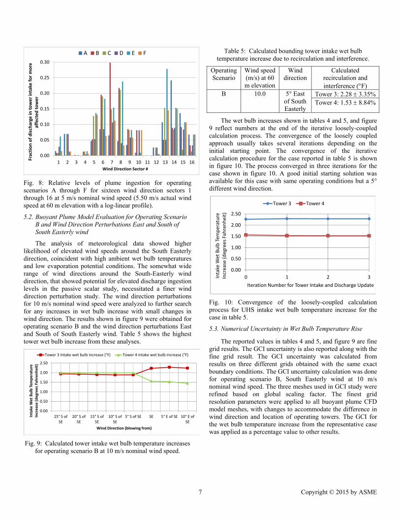
Fig. 8: Relative levels of plume ingestion for operating scenarios A through F for sixteen wind direction sectors 1 through 16 at 5 m/s nominal wind speed (5.50 m/s actual wind speed at 60 m elevation with a log-linear profile).
5.2. Buoyant Plume Model Evaluation for Operating Scenario B and Wind Direction Perturbations East and South of South Easterly wind
The analysis of meteorological data showed higher likelihood of elevated wind speeds around the South Easterly direction, coincident with high ambient wet bulb temperatures and low evaporation potential conditions. The somewhat wide range of wind directions around the South-Easterly wind direction, that showed potential for elevated discharge ingestion levels in the passive scalar study, necessitated a finer wind direction perturbation study. The wind direction perturbations for 10 m/s nominal wind speed were analyzed to further search for any increases in wet bulb increase with small changes in wind direction. The results shown in figure 9 were obtained for operating scenario B and the wind direction perturbations East and South of South Easterly wind. Table 5 shows the highest tower wet bulb increase from these analyses.
Fig. 9: Calculated tower intake wet bulb temperature increases for operating scenario B at 10 m/s nominal wind speed.
Table 5: Calculated bounding tower intake wet bulb temperature increase due to recirculation and interference.
Operating Scenario
Wind speed (m/s) at 60 m elevation
Wind direction
Calculated recirculation and interference (F)
B 10.0 5° East of South Easterly
Tower 3: 2.28 3.35% Tower 4: 1.53 8.84%
The wet bulb increases shown in tables 4 and 5, and figure 9 reflect numbers at the end of the iterative loosely-coupled calculation process. The convergence of the loosely coupled approach usually takes several iterations depending on the initial starting point. The convergence of the iterative calculation procedure for the case reported in table 5 is shown in figure 10. The process converged in three iterations for the case shown in figure 10. A good initial starting solution was available for this case with same operating conditions but a 5° different wind direction.
Fig. 10: Convergence of the loosely-coupled calculation process for UHS intake wet bulb temperature increase for the case in table 5.
5.3. Numerical Uncertainty in Wet Bulb Temperature Rise
The reported values in tables 4 and 5, and figure 9 are fine grid results. The GCI uncertainty is also reported along with the fine grid result. The GCI uncertainty was calculated from results on three different grids obtained with the same exact boundary conditions. The GCI uncertainty calculation was done for operating scenario B, South Easterly wind at 10 m/s nominal wind speed. The three meshes used in GCI study were refined based on global scaling factor. The finest grid resolution parameters were applied to all buoyant plume CFD model meshes, with changes to accommodate the difference in wind direction and location of operating towers. The GCI for the wet bulb temperature increase from the representative case was applied as a percentage value to other results.
0.00
0.05
0.10
0.15
0.20
0.25
0.30
1 2 3 4 5 6 7 8 9 10 11 12 13 14 15 16
Fraction of discharge in
tower intake for more
affected tower
Wind Direction Sector #
A B C D E F
0.00
0.50
1.00
1.50
2.00
2.50
25° S ofSE
20° S ofSE
15° S ofSE
10° S ofSE
5° S of SE SE 5° E of SE 10° E ofSE
Intake W
et Bulb Tem
perature
Increase (degrees Fah
renheit)
Wind Direction (blowing from)
Tower 3 intake wet bulb increase (°F) Tower 4 intake wet bulb increase (°F)
0.00
0.50
1.00
1.50
2.00
2.50
0 1 2 3Intake W
et Bulb Tem
perature
Increase (degrees Fahrenheit)
Iteration Number for Tower Intake and Discharge Update
Tower 3 Tower 4
7 Copyright © 2015 by ASME

6. CFD MODEL RESULTS
The calculation of bounding case interference and recirculation considered wind directions and operating scenario combinations that were selected using a passive-scalar dispersion study to identify potential high interference and recirculation cases. The results of the external plume dispersion show that the interference and recirculation is very dependent on external wind direction, wind speed and the configuration of operating towers. The relative levels of interference and recirculation show strong urban terrain effects which define the flow field. The following operating scenarios and wind direction sectors were identified as high recirculation and interference cases based on dispersion study with 5 m/s nominal wind speed (at 60m elevation).
Operating Scenario B, Wind direction 007 (SE wind)
Operating Scenario E, Wind direction 013 (W wind) The identified cases were evaluated further using the
buoyant plume CFD model. The loosely-coupled calculation process converged quickly in three updates for most cases with a good initial starting point. The operating scenario B, wind direction sector 7 (South Easterly wind) was further examined by varying the wind angle in smaller steps of ±5º to establish bounding recirculation and interference wet bulb increase at tower intake as 2.28 3.35% for 5° East of South Easterly wind at 10 m/s nominal wind speed. The GCI method is used to calculate numerical uncertainty in reported wet bulb temperature increases at the tower intake. The input uncertainty is not considered for simulation results as inputs were chosen as bounding (maximum heat load, minimum plume buoyancy, high ambient wet bulb temperature, and steady basin temperature), or varied (wind speeds, operating scenarios, wind directions) to get the bounding result.
The results for actual intake wet bulb temperature increases calculated correlate with the passive scalar study predictions. The passive scalar study captured the broad peak for operating scenario B around the South Easterly wind direction. The operating scenario E, wind direction sector 13 was also identified as an elevated recirculation and interference case. Buoyancy contributes to additional plume dilution for cases with larger separation of upstream and downstream operating towers.
7. CONCLUSIONS
An incompressible formulation using commercial CFD code has been verified and validated against published experimental data. This has addressed the requirements of NQA-1 Quality Assurance as well as the ASME V&V 20-2009 guidelines. The validation cases individually addressed sub-sets of the actual problem physics but did not have all relevant non-dimensional numbers simultaneously at the actual application scale. A more complete assessment of the scale and the interaction effects in the significant non-dimensional numbers is facilitated by availability of appropriate model test data, or
full scale data from a similar configuration. If direct measurements of validation metric at or near scale are not available, an assessment of the model error in calculated results will require sophisticated roll-up techniques.
The results of the external dispersion show that the interference and recirculation is very dependent on external wind direction, speed and configuration of operating towers and cells. This is expected in dense urban terrain with large buildings. The complex flow patterns associated with particular NPP layout require accurate assessment of recirculation and interference with 3-D CFD techniques or test measurements at appropriate scale.
The bounding value for tower recirculation and interference is calculated as 2.28º F 3.35%. This is based on worst operating scenario-wind direction combination, maximum realistic sustained wind speed (expected to be less than 10 m/s), peak accident heat release, and minimum limiting plume buoyancy. The result supports a decoupled UHS sizing and design assessment which uses an intake wet bulb correction to calculate UHS system response to an accident.
8. NOMENCLATURE
ReD = buoyant jet Reynolds number FrD = buoyant jet Froude number = buoyant jet to wind velocity ratio = ambient stratification parameter ReH = Reynolds number for flow over bluff body β = thermal expansion coefficient = potential temperature v = virtual potential temperature v
r = reference virtual potential temperature T = absolute temperature P0 = reference pressure P = pressure = density 0 = reference density R/Cp = gas constant to specific heat ratio for dry air q = water vapor mass fraction Ui = ith velocity component xi = ith spatial coordinate t = time = molecular momentum diffusivity T = turbulent momentum diffusivity = molecular thermal diffusivity = molecular mass diffusivity of water vapor in air uτ = friction velocity for flow over no-slip surface PrT = turbulent Prandtl number ScT = turbulent Schmidt number E = model bias or comparison error S = simulation result D = experimental measurement unum = uncertainty due to numerics uinput = uncertainty due to inputs uD = uncertainty in experimental data uval = validation uncertainty
8 Copyright © 2015 by ASME

s = signed simulation error model = signed model error input = signed input error num = signed numerical error Fs = Factor of safety for GCI calculation GCI = Grid Convergence Index ij = Kronecker delta
= forced plume momentum length scale = forced plume buoyancy length scale
9. ACKNOWLEDGMENTS
The authors would like to acknowledge the contributions of Solomon Abdi, Natasha Jones, Kathryn Richards, and Jeff Tracewski from Bechtel Corporation.
10. REFERENCES
1. Sullivan, S. M. and Dunn, W. E., Method for Analysis of Ultimate Heat Sink Cooling Tower Performance, Performed for U.S. Nuclear Regulatory Commission, April 1986, Accession Number ML12146A145.
2. Zheng, D., Jarvis, J. M., and Vieira, A. T., Assessing the Design Margins for an Ultimate Heat Sink Sizing, Paper No. ICONE 21-16396, Proceedings of the 21st International Conference on Nuclear Engineering, Chengdu, China, July 29- August 2, 2013.
3. Jirka, G. H., Integral Model for Turbulent Buoyant Jets in Unbounded Stratified Flows, Part 1: Single Round Jet, Environ. Fluid Mech., v 4, 2004.
4. Chu, V. H. and Goldberg, M. B., Buoyant Forced-Plumes in Cross Flow, ASCE J. Hydraulics Division, 100, 1203-1214, 1974.
5. Lim, H. C., Castro, I. P., and Hoxey, R. P., Bluff Bodies in Deep Turbulent Boundary Layers: Reynolds-number Issues, J. Fluid. Mech., 571(1), 2007.
6. Sorbjan, Z., The Large-Eddy Simulations of the Atmospheric Boundary Layer. Chapter 5B of Air Quality Modeling - Theories, Methodologies, Computational Techniques, and Available Databases and Software, Vol. II – Advanced Topics. (P. Zannetti, Editor), 2004. Published by The EnviroComp Institute (www.envirocomp.org) and the Air & Waste Management Association (www.awma.org).
7. Lindenburg, M. R., Mechanical Engineering Reference Manual, 12th ed., Professional Publications Inc., Belmont, California, 2006.
8. Buck, A. L., New Equations for Computing Vapor Pressure and Enhancement Factor, Journal of Applied Meteorology, v 20, December 1981.
9. Huang, P. H., Thermodynamic Properties of Moist Air Containing 1000 to 5000 PPMV of Water Vapor, Proceedings of the RL/NIST Workshop held at the National Institute of Standards and Technology, Gaithersburg, MD, April 5-7, 1993.
10. Lemmon, E. W., Jacobsen, R. T., Penoncello, S. G., and Friend, D. G., Thermodynamic Properties of Air and Mixtures of Nitrogen, Argon and Oxygen from 60 to 2000 K at Pressures to 2000 MPa, Journal of Physical and Chemical Reference Data, v 29, n 3, 2000.
11. Wagner, W. and Pruss, A., International Equations for the Saturation Properties of Ordinary Water Substance. Revised According to the International Temperature Scale of 1990; Addendum to Journal of Physical and Chemical Reference Data, 16, 893 (1987), v 22, n 3, 1993.
12. Reid, R. C., Prausnitz, J. M., and Sherwood, T. K., The Properties of Gases and Liquids, 3rd ed., McGraw-Hill Book Company, New York, 1977.
13. Cooling Tower Manual, Chapter 2, Introduction to CTI Thermal Design, Cooling Tower Institute, 1998.
14. Feltzin, A. E. and Benton, D., A More Nearly Exact Representation of Cooling Tower Theory, Paper No. TP91-02, CTI Annual Meeting, New Orleans, Louisiana, February 6 to 8, 1991.
15. Kloppers, J. C. and Kroger, D. G., Cooling Tower Performance: A critical Evaluation of Merkel Assumptions, R&D Journal, 20(1), 2004.
16. STAR-CCM+ User Guide, Version 7.04.006, CD-Adapco, 2012.
17. Standard for Verification and Validation in Computational Fluid Dynamics and Heat Transfer, ASME V&V 20, 2009 edition.
18. Roache, P. J., Fundamentals of Verification and Validation, Hermosa Publishers, 2009.
19. Martinuzzi, R. and Tropea, C., The Flow Around Surface-Mounted, Prismatic Obstacles Placed in a Fully Developed Channel Flow, ASME Journal of Fluids Engineering, v 115, 1993.
20. Iaccarino, G., Ooi, A., Durbin, P. A., and Behina, M., Reynolds Averaged Simulation of Unsteady Separated Flow, International Journal of Heat and Fluid Flow, 24(2), 2003.
21. Hussein, H. J. A. and Martinuzzi, R. J., Energy Balance for Turbulent Flow Around a Surface Mounted Cube Placed in a Channel, Physics of Fluids, 8(3), 1996.
22. Richards, P. J., Hoxey, R. P., and Short, L. J., Wind Pressures on a 6m Cube, Journal of Wind Engineering and Industrial Aerodynamics, 89(14-15), 2001.
23. Richards, P. J., Hoxey, R. P., Connell, B. D., and Lander, D. P., Wind-tunnel Modeling of the Silsoe Cube, Journal of Wind Engineering and Industrial Aerodynamics, 95(9-11), 2007.
24. Easom, G., Improved Turbulence Models for Computational Wind Engineering, Doctoral Dissertation, University of Nottingham, January 2000.
25. Meroney, R. N., CFD Prediction of Cooling Tower Drift, Colorado State University, 2005.
26. Blevins, R. D., Applied Fluid Dynamics Handbook, Krieger Publishing Company, Malabar, Florida, 2003.
27. Fan, Loh-Nien, Turbulent Buoyant Jets into Stratified or Flowing Ambient Fluids, Report No. KH-R-15, June 1967.
9 Copyright © 2015 by ASME

ANNEX A
VALIDATION OF BUOYANT PLUME CFD MODEL
A.1 Buoyant Plume CFD Model Settings
A steady state solver is suitable for performing buoyant plume simulations using the loosely-coupled calculation process. The buoyant plume CFD model is constant density incompressible flow model that uses the segregated solver based on SIMPLE algorithm. The far field wind velocity and turbulence profiles are calculated from an equilibrium boundary layer model as explained in section 4.4. The convection scheme for all transported variables is second order upwind with slope limiters. The diffusion fluxes and pressure gradients are calculated with second order accuracy. The solutions are run in steady state. The mesh used in the solver is a polyhedral mesh with prism layers on all walls to resolve the boundary layer profile. The turbulence model used was the realizable model with enhanced wall treatment (EWT). The EWT is a hybrid approach based on two-layer Wolfstein shear driven formulation and wall function approach based on blended near wall profiles. The turbulence model includes modification to account for thermal buoyancy. This model converges well in steady state for the buoyant plume simulation, and the computational cost is only marginally higher than the standard
model.
A.2 Code Verification and Validation
The commercial code STAR-CCM+ is used in this study (Ref. 16). Bechtel calculation procedures require compliance with NQA-1 and additional requirements before software can be used for nuclear safety related calculations. It is required that STAR-CCM+ capabilities required to solve the current problem be tested by solving problems with experimental data or known results. As part of the validation exercise several test problems were identified and simulated using STAR-CCM+. The numerical solutions were compared to measured experimental data and the validation error was determined (Ref. 17, 18). The verification and validation (V&V) effort follows ideas outlined in the ASME V&V 20-2009 Standard. The method involves three steps, code verification, solution verification, and solution validation to quantify model bias and uncertainty in predicted output. The verification and validation metrics are quantified estimates of the model bias, , and of the validation uncertainty, as explained below.
DSE (A-1)
222Dinputnumval uuuu (A-2)
∈ , (A-3)
A.3 Specific Test Problems
The test problems listed in table A-1 were simulated in steady state to determine the comparison error in the physical parameter range of interest. For the validation, is calculated using results from three grids. The is calculated based on scatter in data. The input uncertainty is set to
zero as the inputs were known well or, the simulation results of interest (non-dimensional solution variables) were insensitive to small variations in physical input values. The calculations ensured that results were not sensitive to the domain sizes. The inlet profiles for far field ambient wind were calculated based on equilibrium boundary layer for atmospheric external flows. For wall bounded flows, reasonable values for turbulence levels were prescribed at the inlets and the domain included adequate upstream section for the incoming flow to develop.
Table A-1: Summary of validation test problems.
Description Non-dimensional
parameter
Validation metric(s)
1 Turbulent flow over a cube in fully
developed channel flow with channel
height equal to twice the height (Ref. 19-
21)
4 4 Rear flow reattachment
length
2 Atmospheric flow over 6 m cube placed
on open flat terrain (Ref. 22-24)
4.1 6 Rear flow reattachment
length
3 Laboratory scale negatively buoyant
sinking plumes (Ref. 4) – simulated using
full scale, case 4 CFD model for positively
buoyant rising plume, with appropriate
change in conditions to match experimental
parameters
⁄0.7354.1710.8
representing gradual
transition from buoyancy
dominated to strongly forced
plumes
Plume rise
4 Full scale buoyant plume in cross flow –
Chalk Point Tracer Study (1977), 27.4m
diameter stack discharge at 124m
above grade (Ref. 25).
0.56 7.4 6 0.96
0 ( ⁄ 1.26
Plume rise and plume
spread
A.4 Validation Results
For the cases 1 and 2 in table A-1, we have significant model bias that exceeds the validation uncertainty. The causes of the model bias include the steady state assumption and intrinsic turbulence model shortcomings with respect to separated external flow. The flow coming on to the cube separates at the sharp edges on the front face and the flow reattachment and pressure recovery is sensitive to predicted levels of turbulence. It is common to have errors in prediction of flow reattachment lengths in the range of several tens of percentages. Thus, somewhat elongated wake recirculation regions are expected with the buoyant plume CFD model.
A very substantial improvement in rear reattachment lengths for cases 1 and 2 was obtained by employing the
10 Copyright © 2015 by ASME

turbuHowedue tdischsupprsensit
Fcorreluncercorrelwith plumeThe ccondiscale condistrongthat concewithinlocatiresult
correldiscer
Fflow trajecRef. input plumeplume300m2 androtatipossiboscillsmearintermcompplume
A.5 V
Ttable flow The reattaThe mcases limitaflowscrucia
ulence suppressever, this optioto the presenc
harge close toression on wativity study in tFor case 3, tlations and ertainty is neglations provideexperiments f
es with significase 4 full scitions, was useplumes with
itions graduallygly forced plusimulation re
entration in tn (avions) of the cots for plume ri
, are withinlations in Rerned and the si
For case 4, whshown in figu
ctory compared4. The concluuncertainty w
e spread rate pe concentration
m downstream sd A-3. The plumng vortices. Eably due to slatory plume nrs the edge mittency. The ppares well withe widths.
Validation Conc
The validationA-2. A steadyaround buildisimulation re
achment lengthmodel bias fa 1 and 2 is atations of the s. Accurately sal to the accura
sion option in on may not be ce of the veryo building waall boundaries the real applicathe simulationexperimental glected for caed in Ref. 4 gfor buoyancy icant discrepanale CFD moded to simulate ⁄ 0.735
y transitioningumes. The comesults for pluthe plume crverage % orrelation in Rise and the assn the data scaf. 4. Thus, nimulation resulhich is a full sre A-1, the simd well to preusions were si
was also neglecprediction wasn and in-planesections of the me cross-sectioarly plume radsmearing in thnear the stackof the plum
plume radius ah correlations
clusions
n error and moy state CFD mngs and for fsults compare
h behind a cubar exceeding tttributed to ste
turbulence msimulating theacy of the resul
the realizableusable in the
y high Reynolalls. The use
is only recoation. n results weredata in Ref.
ase 3 validatigenerally produ
dominated anncies for plum
del with changthree cases fo5, 4.17 10g from buoyancmparison of thume rise (heiross-section ce
for severaRef. 4. The casociated numeratter of the exno significant lts are boundedscale buoyant pmulation resultdictions from imilar to casected for the cas evaluated bye velocity profi
plume as showon shows the e
dius over prediche RANS av
k. The RANS me that is chat 300m downs
for characteri
odel bias are model has beeforced plumes e well with dbe in validationthe validation
eady state assumodel for extee plume spreadlts sought in th
e modereal applicatiolds number fa
of turbulencommended as
e compared t4. The inpu
ion study. Thuce good matcnd forced drames in betweenges to boundarr the laborator.8, representincy dominated the data showeight at higheenterline) weral downstreamse 3 simulatiorical uncertaintxperiments anmodel bias i
d by data. plume in crossts for the plum
correlations i 3 results. Thse 4 study. Th
y examining thfile at 100m anwn in figures Aexpected contraction at 100m
veraging of thaveraging als
haracterized bstream locationistic radius an
summarized ien validated fo
in cross-flowdata except fon cases 1 and 2n uncertainty iumption and thernal separated is considere
his study.
el. on an ce a
to ut he ch aft n. ry ry ng to ed st re m on ty nd is
s-me in he he he nd A-a-is
he so by ns nd
in or s. or 2. in he ed ed
Fig. A
Fig. Avector
Fig. AcharacAmeriGauss
A-1: CFD mod
A-2: Plume disrs at vertical pl
A-3: Plume sprcteristic radius ican Meteorolosian plume mod
del of large scal
scharge concenlane 100m dow
read from CFD(white dashed
ogical Societydel use recomm
le plume in ope
ntration and inwnstream of rel
D model compd circle) and they’s 1977 reviewmendation (bla
en flat terrain.
n-plane velocitylease location.
pared to Ref. 4e application ow (Ref. 26) on
ack solid oval).
y
4 of n
11 Copyright © 2015 by ASME

Table A-2: Summary of validation results.
Description Validation metric
Maximum validation
uncertainty,
(% of data)
Model bias,
(% of data)
1 Cube in channel experiment
Rear reattachment
length to cube height ratio
±17.6% +66.2%
2 6m cube in open terrain
Rear reattachment
length to cube height ratio
±18.1% +100%
3 Laboratory scale plumes
(Ref. 4),
⁄0.7354.1710.8
Plume rise ±8.5% ±10.6% ±12.1%
| |
4 Buoyant plume in cross flow (Chalk Point,
1977)
Plume rise ±8.5% | |
Plume spread rate
- Qualitative validation of flow pattern - Good comparison to plume cross-section radius
ANNEX B
INTERPRETATION AND VALIDATION OF PASSIVE SCALAR STUDY
B.1 Defining a Threshold Recirculation and Interference
The tower discharge spreadsheet calculation was used to calculate the volumetric level of tower discharge recirculation at the cooling tower intakes, which would cause the maximum tolerable wet bulb increase (available from decoupled UHS accident analysis). The threshold value is 12% for the chosen ambient conditions and heat load used. This threshold value conservatively neglects the buoyancy of the saturated plume.
The associated simulation error (δs = δnum + δinput + δmodel) for the computational results shown in figure 8 needs to be calculated. Numerical uncertainty in the passive scalar study was determined by computing the time averaged transient results on two grids for same time step size, and for two different time step sizes on the same grid. GCI numerical uncertainty is calculated in table B-1 with assumed order of convergence for space and time. The variable of merit in our simulation is the time averaged flux of passive scalars into the tower intakes. The solution method is a mixed order method with minimum discretization order being first order. The Factor of Safety in GCI calculation, Fs is taken as 1.25 along with assumed order of convergence of 1 in time and space. The combined GCI is calculated by adding the coarse grid and larger time step GCI’s in time and space. δnum is bounded as
29.5% . The equal plume discharges imposed at all the tower fan
discharges in the passive scalar study, can introduce some error in the evaluation due to the extra flow inlets and outlets existing
at non-operating towers. The input error on account of having all towers flowing is bounded by calculating the difference in predicted interference and recirculation in the operating case and wind direction expected to be most affected by flows into and out of non-operating towers. Table B-2 shows the input error in passive scalar ingestion from having all towers operating for operating scenario E, wind direction sector 13.
Table B-1: Calculation of GCI numerical uncertainty from two grid and two time step study for operating scenario B, with 5 m/s nominal wind speed and wind direction sector 007.
Number of facets in Tower
3 and 4 intakes
Number of facets in Tower 3
and 4 discharges
Plume ingestion for
most affected
tower
Time step size
Number of iterations per time
step/ sampling
period Temporal GCI calculation
Baseline grid # 0
627 181 0.2986 1.0 s 20/50s
Baseline grid # 0
627 181 0.2899 0.5 s 25/50s
Extrapolated value=0.2812 using refinement ratio, r=2.0
Temporal GCIcoarse = 0.0218
Spatial GCI calculation Baseline grid # 0
627 181 0.2823 0.5 s 25/100 s
Fine grid # 1
1321 254 0.2658 0.5 s 25/100 s
Extrapolated value = 0.2127 using refinement ratio, r=1.31§
Spatial GCIcoarse
=0.0663
Combined GCI and unum calculation Combined GCIcoarse
0.0881
0.0881 29.5%
§ using the geometric mean of the spatial refinement ratios at two significant locations
The model error includes errors caused by modeling assumptions, the most significant one being the turbulence model. The validation exercise establishes the range of model error for the validation problems as ∈ ,
.
B.2 Passive Scalar Study CFD Model Settings
The CFD model for passive scalar study used a coupled implicit formulation based on ROE-FDS scheme. The solver employs preconditioning for low speed flows. The unblended form of ROE-FDS scheme is chosen with the discretization option set to first order. The turbulence and passive scalar transport equations use a second order accurate convection scheme with slope limiters. The molecular Schmidt number for all the passive scalars is set to 0.9. The diffusion flux evaluation is second order accurate. The flow is modeled as unsteady and the temporal discretization is first order implicit. The turbulence model used is non-linear cubic version of turbulence model with low Reynolds number effects and an all
near wall treatment. The Durbin scale limiter is used to limit eddy viscosity in stagnation regions. The turbulence model required time accurate solution, and use of lower order convection scheme for the momentum equation to solve high
12 Copyright © 2015 by ASME

Reynto comfor thlayersis takcalcuprofil
Tablein pa
T
TowTow
B.3 V
T6m cua labdownbuoyaforcedas timflow w
Fscalar
Awall rin ope
Fliquidmiscibasedwas utranspwith 100 fvolumturbubuoyais noApprospeciffree sdown
Fcriterin theB-4 simulresult
olds number flmpare to expehe passive scas on all wall boken as a log-
ulated from a 2le as explained
e B-2: Calculatassive scalar stu
wind spe
Tower Calc
ingestioall ope
wer 3 wer 2
Validation Resu
Two validationube in open ter
boratory scale nwards (Ref. 2ant forced plud plume disch
me accurate anwas establishe
Following chanr CFD model sA hexahedral mresolution is usen terrain. For simulatingd and lighter aible liquids. Thd on SIMPLE aused for momport equationsslope limiters.
for the jet fluidme fractions oulence kinetic ancy productio
ot needed for opriate constafied at the inlsurface was monward jet also uFigures B-1 anria iso-surfacese flow around tshow results
lation. Table Bts to the exper
flows. Simulatierimental data.alar study is a oundaries. The-linear profile 24 km long dod in section 4.7
tion of fudy for operatieed and wind d
culated plume
on with towers erating
plummo
onlytowe
0.278 0.019
ults
n cases are run,rrain (Ref. 22-negatively bu
27). The dowume is equivaharged upwardnd the results d. nges were madsettings for runmesh with appsed for the vali
the negativelambient streamhe solver was algorithm and
mentum. The ts used a seco The moleculad. A user definof the liquidsenergy sourc
on of turbulencthe constant
ant values of let flow boundodeled as a slipused a hexahednd B-2 show
s identifying ththe 6m cube in
for the negB-3 compares rimental measu
on results wer The mesh usepolyhedral m
far field wind and turbulen
omain with log.
for having all toing scenario E,direction sector
Calculated e ingestion
odeled with y operating ers flowing
E
in
0.243 0.021
, first being th24), and the seuoyant jet tha
wnward discharalent to a posds. Both simula
were time ave
de with respecnning the validapropriate bounidation studies
ly buoyant jet m liquid are mchanged to sefirst order con
turbulence andnd order convar Schmidt numned mixture ds was used. Ace term was ce. The additiodensity passivturbulence pa
dary on the tesp wall. The negdral mesh.
the streamlinhe expected von open terrain. Fgatively buoya
the plume deurements. The
e time averageed in the solve
mesh with prismvelocity profil
nce profiles arg-linear velocit
owers operatin, 5 m/s nominar 13.
Estimated
Plume ngestion
level
(%)
0.035 12.60.002 10.5
e flow around econd one beinat is dischargerged negativelsitively buoyanations were rueraged after th
ct to the passivation problemsndary layer nea
with a 6m cub
the heavier jemodeled as twegregated solvenvection schemd mass fractiovection schemmber was set tensity based oAdditionally, used to mode
onal source termve scalar studyarameters werst channel. Th
gatively buoyan
nes and the Qortical structureFigures B-3 anant sinking jeepth and radiuplume depth
ed er m le re ty
ng al
)
6 5
a ng ed ly nt un he
ve . ar be
et wo er
me on me to on
a el m y. re he nt
Q-es nd et us is
calculpeaks boundin excconcenas thconcencorrelaReynorelativ
B.4 Va
Ttable Baroundsimulamodelof theThe Cfrom cbelievmodelvalidaoperatconsid
Fig: Bhorizocoloreapproa
lated as the avon the plum
ding dimensioncess of 50% ntration peakse inverse of ntration peaksation. Both tolds number flvely finer mesh
alidation Conc
The validation B-4. An unstead buildings anation results cl bias is observe plume preserCFD predictiocorrelations in
ved to a resulling approachation results, tting scenario dering any con
B-1: Constraineontal (bottomed by static preaching flow dir
verage depth ome section. Thns of the plume
of the averas. The plume cf the averages, is comparedthe validationows than the p
hes than the pa
clusions
error and moady CFD modend for forced compare well ved except for rves higher coons agree bett
Ref. 4. The dilt of the aver
h and experimthe passive sc– wind direct
ntributions from
ed streamline pplot) section
essure showingrection is show
f the two locae plume radiu
e section havinage value ofcenterline dilute concentratiod to experimen problems inpassive scalar sssive scalar stu
odel bias are el has been val
plumes in crwith data andthe plume dilu
oncentration thter with dilutiiscrepancy withraging in RA
mental errors.calar ingestiontion study are
m model error.
plot on verticans through thg the time averwn by the arrow
al concentrationus is based ong concentrationthe two loca
tion, calculatedn at the tw
ent and Ref. 4nvolved lowestudy, and usedudy.
summarized inlidated for flowross-flows. Thd no significanution. The cor
han experimention predictionh experiment i
ANS turbulencBased on th
n results in the used withou
al (top plot) anhe cube centeraged flow. Thw.
n n n al d o 4
er d
n w e
nt e t.
ns is e e e
ut
d er e
13 Copyright © 2015 by ASME

Fig. BvisuaThe a
Fig. plumelocatidown
TableCFD . i
point,
⁄
414396289
119
B-2: Vortical alized by Q-criapproaching flo
B-3: Plume me with cross-flions of maximnstream distanc
e B-3: Compariresults (S) fors plume radiu, and is the in
⁄ ⁄ (S)
⁄(D
4.1 4.8 54.3 8.7 99.0 13.5 132.2 17.0 169.0 19.6 209.0 22.9 24
structures arouiteria isosurfacow direction is
mass fraction ow from right um concentrat
ces from the rel
ison of experimr sinking jet teus, is downnitial plume di
⁄ D)
. ⁄ (S)
. (
.8 2.08 1
.0 2.51 2
.6 4.49 3
.5 5.15 4
.8 7.10 5
.8 9.25 8
und the cube ces colored by
shown by the
contours on sto left. Points
tion measuremlease point (Re
mental measureest case. is thstream distanciameter at relea
⁄(D) (S)
.04 2.3 2.20 5.1
.00 11.6 4.40 17.4 5.90 24.9 8.80 34.5
in open terraistatic pressurearrow.
section throug1 through 6 arents at differenef. 27).
ements (D) withe plume depthce from releasase point.
(D)
6.0 8.15.0 13.30.0 20.38.0 25.57.0 31.69.0 36.
in e.
gh re nt
th h, se
. 4.
.4
.3
.6
.8
.1
.5
Fig. concenplume
Table
Va
6 mopen
exp
Negb
sinkincro
(
B-4: Verticalntration and
e mass fraction
B-4: Summary
alidation case
m cube in n terrain,
Silsoe periment 4.1 6
reattac
Cp reon sid
– minimmaximmeasu
lo
Cp reon
minimmaximmeasu
logatively buoyant ng jet in oss-flow
3.988200100
⁄6.77
Jet traj
cend
l sections thrin-plane veloc
n on the section
y of validationstudy CFD
Metric Experimmeasur
Rear chment length
1.2cube
(Reecovery de faces mum to
mum for urementocations
0.54front t
(Re
ecovery n roof –mum to
mum forurementocations
0.612front t
(Re
jectory, radius,
nterline dilution
R
rough the plcity vectors. n is noted on th
n test results formodel.
mental rement
(D)
Simulatiresult
to 1.4 height ef. 24)
1.174 cuheig
4 from to rear ef. 22)
0
2 from to rear ef. 22)
0
Ref. 27 trajectoradius,
plavelocfield
plumcro
secti
lume showingThe maximum
he scale.
r passive scala
ion (S)
Model bias
ube ght
No significb
.45 Closeexperimen
pressrecovery fr
front to rearcenterline
side fa.34 Wea
pressrecovery
roof– recovcontinues
back fJet
ory, in-
ane city
on me
oss-ion
No significbias except plume dilut
g m
r
s, E
ant bias
e to ntal ure om on
e of ces ker ure on
ery on
faceant for ion
14 Copyright © 2015 by ASME

B.5 Operating Scenarios and Wind Directions with Potentially High Recirculation and Interference Levels
The following operating scenario and wind direction sectors were identified for further evaluation using a buoyant plume CFD model:
Operating Scenario B, Wind direction sector 007 Operating Scenario E, Wind direction sector 013
The selection of these cases was based on following considerations: i. For conservatism in picking up the operating scenarios and
wind directions, s for figure 8 results is calculated as
. ∈ 32.1%
Based on this, operating scenarios and wind directions with tower discharge ingestion level less than 0.091 in figure 8 are not considered further.
ii. The likelihood of persistent wind speeds exceeding 2.5 m/s in the different directions (from site specific wind rose) in high ambient wet bulb temperature and low evaporation potential conditions.
iii. Some cases will likely see more benefit from plume buoyancy because of separation of the upstream and downstream towers.
iv. The similarity in flow configurations is used to reduce the number of cases that need to considered
v. Wind speed and direction sensitivity of selected operating scenarios and wind directions was also considered in selecting cases for further evaluation. The sensitivity for operating scenarios B and E (with non-operating towers not flowing) is shown for wind speeds ranging from 1 m/s to 20 m/s in figures B-5 and B-6 respectively. Operating scenario B, wind direction sector 7, and operating scenario E, wind direction sector 13 were compared to adjacent directions (±22.5º) at a higher nominal wind speed of 10m/s. This confirmed that they were higher plume ingestion cases compared to adjacent wind directions as shown in figures B-7 and B-8.
Fig. B-5: Sensitivity of plume ingestion to wind speed for operating scenario B and wind direction sector 007.
Fig. B-6: Sensitivity of plume ingestion to wind speed for operating scenario E and wind direction sector 013.
Fig. B-7: Sensitivity of plume ingestion to wind direction for operating scenario B at 10 m/s nominal wind speed.
Fig. B-8: Sensitivity of plume ingestion to wind direction for operating scenario E at 10 m/s nominal wind speed.
0.00
0.05
0.10
0.15
0.20
0.25
0.30
0.35
0.40
1.0 2.5 5.0 10.0 20.0
Fraction of discharge in
tower intake for more
affected tower
Nominal wind speed (m/s)
Operating Scenario B ‐Wind Direction Sector 007
0.00
0.05
0.10
0.15
0.20
0.25
0.30
0.35
0.40
1.0 2.5 5.0 10.0 20.0
Fraction of discharge in
tower intake for more
affected
tower
Nominal wind speed (m/s)
Operating Scenario E ‐Wind Direction Sector 013
0.00
0.05
0.10
0.15
0.20
0.25
0.30
0.35
0.40
#006 #007 #008
Fraction of discharge in
tower intake for more
affected tower
Wind direction sector #
Operating Scenario B ‐ 10 m/s Nominal Wind Speed
0.00
0.05
0.10
0.15
0.20
0.25
0.30
0.35
0.40
#012 #013 #014
Fraction of discharge in
tower intake for more
affected
tower
Wind direction sector #
Operating Scenario E ‐ 10 m/s Nominal Wind Speed
15 Copyright © 2015 by ASME


![Compact ink recirculation system CC1 - Toshiba Tec Top Page...Compact ink recirculation system Example: Mounting of ink recirculation system [CC1] with ink recirculation head Up to](https://img.pdfslide.net/doc/110x75/5f0f72527e708231d4443441/compact-ink-recirculation-system-cc1-toshiba-tec-top-page-compact-ink-recirculation.jpg)