Embed Size (px)
Citation preview

ASSESSMENT OF FLUCTUATIONAL AND CRITICAL TRANSFORMATIONAL BEHAVIOUR
OF GROUND LEVEL OZONE
NORRIMI ROSAIDA AWANG
UNIVERSITI SAINS MALAYSIA
2015

i
ASSESSMENT OF FLUCTUATIONAL AND CRITICAL
TRANSFORMATIONAL BEHAVIOUR OF GROUND LEVEL OZONE
by
NORRIMI ROSAIDA BT AWANG
Thesis submitted in fulfillment of the requirements
for the degree of
Doctor of Philosophy
August 2015

ii
ACKNOWLEDGEMENTS
In the name of Allah, the Most Gracious and the Most Merciful. Alhamdulillah,
all praises to Allah for the strengths, health and blessing in completing this thesis.
First and foremost, I would like to express my sincerest gratitude to my
supervisor Professor Dr Nor Azam Ramli for the continuous support and guidance of
my research and writing this thesis. His invaluable comments, suggestions, motivation
and enthusiasm are like a force that drive me to complete this study. I could not have
imagined having a better advisor and mentor for my PhD study.
I would like to express special thanks to my co-supervisor, Associate Professor
Ahmad Shukri Yahaya, who provided helpful knowledge, guidance, and suggestions
as well as conscientious review throughout my study. My sincere thanks goes to Dr
Maher Elbayoumi, who as a post doctorate personal, was always willing to help and
give his best suggestions.
My deepest gratitude also goes to my beloved parent, sister and family, who
always there for me. I hope you know how grateful I am for your constant support,
understanding and encouragement along the way of my study.
I would also like to offer my great thanks to the Department of Environment,
Malaysia for providing data for this research and the Ministry of Education Malaysia
for providing financial support to this study under the MyBrain15 program.
Last by not least, special thank are offered to all my friends in Clean Air
Research Group and Postgraduate Room 3 for their valuable friendship, support and
encouragement throughout my research project and to all those who have helped me
in a way or another to make this research a reality.

iii
TABLE OF CONTENTS
Page
ACKNOWLEDGEMENTS
ii
TABLE OF CONTENTS
iii
LIST OF TABLES
ix
LIST OF FIGURES
xi
LIST OF ABBREVIATIONS
xiv
LIST OF APPENDICES
xix
ABSTRAK
xx
ABSTRACT
xxii
CHAPTER 1 : INTRODUCTION
1.1 OVERVIEW
1
1.2 AIR POLLUTION IN MALAYSIA
3
1.3 PROBLEM STATEMENT
8
1.4 OBJECTIVES
12
1.5 SCOPE OF STUDY
12
1.6 THESIS LAYOUT
15
CHAPTER 2 : LITERATURE REVIEW
2.1 INTRODUCTION
16
2.2 GROUND LEVEL OZONE
17
2.2.1 Effect of Ozone 18
2.2.2 Ground Level Ozone Fluctuational Behaviour
20
2.2.3 Ground Level Ozone Transformational Behaviour
22
iv
2.2.3 (a) Daytime Chemistry of Ground Level Ozone Transformation
23
2.2.3 (b) Nighttime Chemistry of Ground Level Ozone Transformation
25
2.2.3 (c) Indices for Ozone formation
27
2.3 OZONE PRECURSORS
31
2.3.1 Nitrogen oxides
31
2.3.2 Volatile organic compounds
34
2.3.3 Carbon monoxide
35
2.3.4 Sulphur dioxide
35
2.4 THE INFLUENCE OF METEROLOGICAL PARAMETERS ON GROUND LEVEL OZONE FORMATION AND FLUCTUATION
36
2.6.1 Influence of Incoming Solar Radiation
37
2.6.2 Influence of Ambient Temperature
38
2.6.3 Influence of Relative Humidity
38
2.6.4 Influence of Wind
39
2.5 MULTIVARIATE ANALYSIS RELATED TO OZONE
40
2.5.1 Principal Component Analysis (PCA)
40
2.5.2 Multiple Linear Regression (MLR)
41
2.5.3 Principal Components Regression (PCR)
43
2.6 SUMMARY 44
CHAPTER 3: METHODOLOGY
3.1 INTRODUCTION
46
3.2 STUDY AREAS AND MEASUREMENT TECHNIQUES
48
3.2.1 Study Areas
48
3.2.2 Weather Condition of Study Areas 54

v
3.2.3 Measurement Techniques
55
3.2.3 (a) Ground Level Ozone
55
3.2.3 (b) Nitrogen dioxide and nitric oxide
57
3.2.3 (c) Sulphur dioxide
58
3.2.3 (d) Carbon monoxide
58
3.2.3 (e) Meteorological Parameters
59
3.2.4 Missing Records
60
3.2.5 Descriptive Statistic Using Box and Whisker Plot
61
3.3 ANALYSIS OF OZONE FLUCTUATIONAL BEHAVIOUR
62
3.3.1 Time Series Plot of Daily Maximum O3 Concentrations
62
3.3.2 Diurnal Plot of Hourly Average O3 Concentrations.
62
3.3.3 Ozone Concentration Map using GIS
63
3.3.4 Exceedances Analysis
65
3.4 ANALYSIS OF OZONE TRANSFORMATIONAL
65
3.4.1 CCP Identification using Composite Diurnal Plot
65
3.4.2 CCP Determination based on O3 Production Rate
66
3.4.3 Verification of O3 Critical Conversion Point in Urban, Sub-Urban and Industrial Areas
66
3.5 DEVELOPMENT OF NEXT HOUR OZONE PREDICTION MODEL
69
3.5.1 ‘Daily’, Daytime, Nighttime and Critical Conversion Time Determination
69
3.5.2 Assessment of Group of Monitoring Stations Based on DoE Classification
70
3.5.3 Developing New Group of Monitoring Stations
71
3.5.3 (a) Ranking of Means
71

vi
3.5.3 (b) Cluster Analysis
73
3.5.4 Principal Component Analysis (PCA)
74
3.5.5 Multiple Linear Regressions (MLR)
78
3.5.6 Principal Components Regressions (PCR)
80
3.6 MODEL VALIDATION AND VERIFICATION
81
3.6.1 Errors and Accuracy Measures
82
3.6.1 (a) Normalized Absolute Error (NAE)
82
3.6.1 (b) Mean Absolute Error (MAE)
83
3.6.1 (c) Root Mean Square Error (RMSE)
83
3.6.1 (d) Index of Agreement (IA)
84
3.6.1 (d) Prediction Accuracy (PA)
84
3.6.1 (e) Coefficient of Determination (R2)
84
CHAPTER 4: RESULTS AND DISCUSSION
4.1 INTRODUCTION
86
4.2 DESCRIPTIVE STATISTIC OF OZONE CONCENTRATION
86
4.3 OZONE FLUCTUATIONAL BEHAVIOUR
89
4.3.1 Daily Fluctuations
90
4.3.2 Diurnal Fluctuations
95
4.3.3 Monthly Fluctuations
99
4.3.4 Spatial Fluctuations
101
4.3.5 Exceedance Analysis of Hourly O3 Concentrations
115
4.4 OZONE TRANSFORMATIONAL BEHAVIOUR
119
4.4.1 Influence of NO2, NO, Temperature and UVB to O3 Formation
120

vii
4.4.2 CCP from Composite Diurnal Plot
134
4.4.3 CCP from Ozone Photostationary State
137
4.4.4 Verifications of O3 Critical Conversion Point
142
4.5 NEXT HOUR OZONE PREDICTION MODEL
147
4.5.1 Group of Monitoring Stations Based on Ozone Concentrations
147
4.5.1 (a) Group Base on DoE classification 148
4.5.1 (b) Ranking of Means Group
149
4.5.1 (c) Cluster Analysis Group 151
4.5.1 (d) Summary of the Groups during Different Ranges of Time
154
4.5.2 Variables Reduction using PCA
155
4.5.3 Multiple Linear Regression Models
161
4.5.4 Principal Component Regression Models
167
4.6 SELECTION OF THE BEST PREDICTION MODELS BASED ON PERFORMANCE INDICATORS
171
4.6.1 Performance Indicators of MLR and PCR Models
171
4.6.2 The Best Prediction Model
175
4.6.3 Comparison between MLR and PCR Models
178
4.6.4 Verification of the Developed Models in Urban, Sub-Urban and Industrial Area
179
CHAPTER 5: CONCLUSION AND RECOMENDATIONS
5.1 CONCLUSION
185
5.2 RECOMMENDATION
188

viii
REFERENCES
189
APPENDICES
LIST OF PUBLICATIONS

ix
LIST OF TABLES
Page
Table 1.1 Malaysian Ambient Air Quality Guidelines
5
Table 1.2 Summary of hourly O3 concentrations exceeding the MAAQG limit of 1-hour averaging around Klang Valley from 2004 to 2008
8
Table 2.1 Characteristics of O3 diurnal trends
21
Table 2.2 Review of daytime and nighttime O3 concentrations
22
Table 2.3 Estimated O3 precursors from stationary, mobile, and biogenic sources in the United States in 1995
31
Table 2.4 Global inventory of NOx sources
33
Table 2.5 Review of O3 prediction models using MLR
42
Table 2.6 Review of developed O3 prediction models using MLR and PCR
43
Table 3.1 Description of the selected monitoring stations
49
Table 3.2 Percentage of missing records for hourly concentration of O3, NO2 and NO during 1999 to 2010
60
Table 3.3 Description of the verification sampling stations
67
Table 3.4 Different time ranges used in the prediction models
69
Table 3.5 One way analysis of variance
70
Table 3.6 Descriptions of newly developed group based on difference in time range
72
Table 4.1 Coefficient of variations of the O3 concentrations
89
Table 4.2 Diurnal mean, maximum concentration and time, diurnal minimum concentration and time and diurnal amplitude of O3 concentrations
97
Table 4.3 Principal component analysis on NO, NO2, temperature and UVB
121
Table 4.4 The time for critical conversion point (CCP) from 1999 to 2010 in all stations
135

x
Table 4.5 Ratio of 2NO 3j k in all stations 139
Table 4.6 Difference in ratio of 2NO 3j k in all stations
140
Table 4.7 ANOVA for original group based on DoE classification
148
Table 4.8 New group of monitoring stations based on ranking of means
150
Table 4.9 Summary of the monitoring stations group based on DoE, ranking of means and cluster analysis during different ranges of time
155
Table 4.10 Principal Components Analysis after varimax rotation for respective group of monitoring stations during AT, DT, NT and CT
156
Table 4.11 Summary of MLR models for O3 concentration prediction for all groups during different time range
162
Table 4.12 Summary of PCR models for O3 concentration prediction for all groups during different time range
168
Table 4.13 Error and accuracy measures for MLR models
172
Table 4.14 Error and accuracy measures for PCR models
174
Table 4.15 The average of 2R value for MLR and PCR model
178
Table 4.16 Verifications of the developed MLR and PCR models in Shah Alam
180
Table 4.17 Verifications of the developed MLR and PCR models in Bakar Arang
181
Table 4.18 Verifications of the developed MLR and PCR models in Nilai
183

xi
LIST OF FIGURES Page
Figure 1.1 Number of registered vehicles in Malaysia 6
Figure 1.2 Annual average concentrations of O3 by land use from
1999 to 2013
7
Figure 3.1 Flow of research methodologies
47
Figure 3.2 Specific location of monitoring stations across Malaysia
50
Figure 3.3 Definition of item in box and whisker plot
61
Figure 3.4 Procedure for developing new groups of monitoring stations using cluster analysis.
73
Figure 3.5 Development of PCA procedures
75
Figure 3.6 Procedure of developing MLR models
78
Figure 3.7 Architecture of a PCR model using PCA outputs as the input to MLR
80
Figure 3.8 Procedure of developing PCR models 81
Figure 4.1 Box and whisker plot of hourly average O3 concentration for all stations
87
Figure 4.2 Time series plot of hourly maximum O3 concentration for Shah Alam, Gombak, Klang, Johor Bahru and Nilai
90
Figure 4.3 Time series plot of hourly maximum O3 concentration for Ipoh, Bukit Rambai, Perai, Bakar Arang, Seberang Jaya and Pasir Gudang
91
Figure 4.4 Time series plot of hourly maximum O3 concentration for Kemaman, Taiping, Kota Bharu, Kota Kinabalu, Kuching and Jerantut
92
Figure 4.5 Diurnal plot of hourly average O3 concentrations in all stations
96
Figure 4.6 (a) Monthly variations of O3 concentrations
100
Figure 4.6 (b) Monthly variations of O3 concentrations
101
Figure 4.7 Monthly maximum O3 concentration map in 1999
102

xii
Figure 4.8 Monthly maximum O3 concentration map in 2000
103
Figure 4.9 Monthly maximum O3 concentration map in 2001
104
Figure 4.10 Monthly maximum O3 concentration map in 2002
105
Figure 4.11 Monthly maximum O3 concentration map in 2003
106
Figure 4.12 Monthly maximum O3 concentration map in 2004
107
Figure 4.13 Monthly maximum O3 concentration map in 2005
108
Figure 4.14 Monthly maximum O3 concentration map in 2006
109
Figure 4.15 Monthly maximum O3 concentration map in 2007
110
Figure 4.16 Monthly maximum O3 concentration map in 2008
111
Figure 4.17 Monthly maximum O3 concentration map in 2009
112
Figure 4.18 Monthly maximum O3 concentration map in 2010
113
Figure 4.19 Annual maximum O3 concentration map from 1999 to 2010 to represent the worst case scenario
114
Figure 4.20 Annual number of exceedances in all stations
115
Figure 4.21 Numbers of exceedances in all stations
117
Figure 4.22 Diurnal variations of O3 exceedances
118
Figure 4.23 Composite diurnal plots of O3, NO2, NO, temperature and solar radiation in Shah Alam, Kajang and Bakar Arang
124
Figure 4.24 Composite diurnal plots of O3, NO2, NO, temperature and solar radiation in Kemaman, Gombak and Nilai
125
Figure 4.25 Composite diurnal plots of O3, NO2, NO, temperature and solar radiation in Bukit Ramba, Ipoh and Perai
126
Figure 4.26 Composite diurnal plots of O3, NO2, NO, temperature and solar radiation in Klang, Johor Bahru and Taiping
127
Figure 4.27 Composite diurnal plots of O3, NO2, NO, temperature and solar radiation in Seberang Jaya, Pasir Gudang and Kota Bharu
128
Figure 4.28 Composite diurnal plots of O3, NO2, NO, temperature and solar radiation in Kota Kinabalu, Jerantut and Kuching
129

xiii
Figure 4.29 Diurnal variations of average 2NO 3j k ratio for all
stations during 1999 to 2010
138
Figure 4.30 Diurnal variations of the O3 concentration in Bakar Arang
142
Figure 4.31 Diurnal plot of verified O3 and NO2 concentrations in Bakar Arang
143
Figure 4.32 Diurnal variations of O3 concentrations in Nilai
144
Figure 4.33 Diurnal plot of verified O3 and NO2 concentrations in Nilai
145
Figure 4.34 Diurnal variations of O3 concentration in Shah Alam
146
Figure 4.35 Diurnal plot of verified O3 and NO2 concentrations in Shah Alam
146
Figure 4.36 The dendrogram of cluster classification of monitoring stations based on O3 concentration during AT, DT, NT and CT
154
Figure 4.37 Scatter plot of observed and predicted O3 concentrations during AT, DT, NT and CT using MLR and PCR models
176
Figure 4.38 Scatter plot of observed and predicted O3 concentration using UB-AT-MLR in Shah Alam
180
Figure 4.39 Scatter plot of observed and predicted O3 concentrations in Bakar Arang using SU-NT-MLR
182
Figure 4.40 Scatter plot of observed and predicted O3 concentrations in Nilai using G2-N-MLR model
184

xiv
LIST OF ABBREVIATIONS
ANOVA Analysis of variance
ANN Artificial neural network
AOT40
Accumulative ozone exposure over a threshold of 40 ppb
AOT50
Accumulative ozone exposure over a threshold of 50 ppb
AOTX Accumulative ozone exposure over a threshold value
AQLVs Air quality limit values
API Air Pollution Index
Ar
Argon
ASMA Alam Sekitar Sdn Bhd
AT Daily
CA Cluster analysis
CAQM Continuous Air Monitoring Stations
CARB
The California Resources Board
CCP Critical conversion point
CEM
Continuous emission monitoring
CH4 Methane
CT Critical conversion time
CO Carbon monoxide
CO2 Carbon dioxide
CV Coefficient of variations
d Durbin-Watson
DT Daytime
DFA Detrended fluctuation analysis
DU Dobson unit

xv
EBIR
Equal benefit incremental reactivity
EQR Environmental quality report (Malaysia)
EU European Union
DoE Department of Environment (Malaysia)
DoSM Department of Statistics (Malaysia)
FEV
Forced expiratory volume
FVC
Forced vital capacity
GDP Gross domestic product
GFC Gas filter correlation
GIS Geographical information system
GSE Gas sensitive electrochemical
GSS Gas sensitive semiconductors
H2
Hydrogen
He
Helium
HO2NO2 Peroxynitric acid
HONO Nitrous acid
HNO3 Nitric acid
hv Radiant energy
HO2 Hydroperoxyl
IA Index of agreement
IAQ Indoor air quality
IR Infrared
JNO2 NO2 photolysis rate
k3 Reaction rate between NO and O3
KMO Kaiser-Meyer-Olkin Measure
xvi
MAAQG Malaysia Ambient Air Quality Guidelines
MAE Mean absolute error
MIR
Maximum incremental reactivity
MLR Multiple linear regression
Mo Molybdenum
MOIR
Maximum ozone incremental reactivity
N2 Nitrogen
N2O
Nitrous oxide
N2O5 Dinitrogen pentoxide
NAAQS National Ambient Air Quality Standards
NAE Normalized absolute error
Ne
Neon
NEM North east monsoon
NO Nitric oxide
NO2 Nitrogen dioxide
NO3 Nitrate
NOx Nitrogen oxides
NRE Ministry of Natural Resources and Environment, Malaysia
NT Nighttime
O
Oxygen atom
O (1D)
Excited single state oxygen atom
O (3D)
Atomic oxygen
O2 Oxygen
O3 Ozone
OFP
Ozone formation potentials

xvii
OH Hydroxyl
OLS Ordinary least square
PA Prediction accuracy
PCA Principal component analysis
PCR Principal component regression
PCs Principal components
PI Performance indicators
PM10 Particulate matter with aerodynamic diameter less than 10 micron
PMT Photomultiplier tube
PNA Poly-nuclear aromatic
POCP
Photochemical ozone creation potentials
ppb
Parts per billion
ppm
Parts per million
R2 Coefficient of determination
2R Adjusted coefficient of determination
RH Relative humidity
RMSE Root mean square error
RO2 Peroxy radicals
SO2 Sulphur dioxide
SO3
Sulphur trioxide
SPSS Statistical Package for the Social Science
SWM Southwest monsoon
T Temperature
TSP Total suspended particulate matter
TVOC Total volatile organic compounds

xviii
USEPA The United State Environmental Protection Agency
UV Ultraviolet
UVB
Ultraviolet with wavelength (290 – 320 nm)
VIF Variance inflation factor
VOCs Volatile organic compounds

xix
LIST OF APPENDICES
Appendix A1 Box and whisker plot of hourly NO2 concentrations during 1999 to 2010
Appendix A2 Box and whisker plot of hourly NO concentrations during 1999 to 2010
Appendix A3 Box and whisker plot of hourly CO concentrations during 1999 to 2010
Appendix A4 Box and whisker plot of hourly SO2 concentrations during 1999 to 2010
Appendix A5 Box and whisker plot of hourly temperature during 1999 to 2010
Appendix A6 Box and whisker plot of hourly UVB intensity during 1999 to 2010
Appendix A7 Box and whisker plot of hourly relative humidity during 1999 to 2010
Appendix B1 Scatter plot of observed and predicted O3 concentrations using AT-MLR models
Appendix B2 Scatter plot of observed and predicted O3 concentrations using DT-MLR model
Appendix B3 Scatter plot of observed and predicted O3 concentrations using NT-MLR models
Appendix B4 Scatter plot of observed and predicted O3 concentrations using CT-MLR models
Appendix B5 Scatter plot of observed and predicted O3 concentrations using AT-PCR models
Appendix B6 Scatter plot of observed and predicted O3 concentrations using DT-PCR models
Appendix B7 Scatter plot of observed and predicted O3 concentrations using NT-PCR models
Appendix B8 Scatter plot of observed and predicted O3 concentrations using CT-PCR models

xx
PENILAIAN TURUN NAIK DAN UBAH TAMPIL TINGKAH LAKU
KRITIKAL OZON PARAS TANAH
ABSTRAK
Ozon paras tanah merupakan pencemar udara yang berbahaya dan berupaya
mendatangkan kesan negatif terhadap kesihatan manusia, hasil tanaman dan alam
sekitar. Pemahaman mengenai ciri-ciri turun naik dan ubah tampil ozon adalah
penting untuk merangka strategi pengurangan dan pengawalan. Oleh itu, kajian ini
dijalankan bertujuan untuk mengenalpasti ciri-ciri turun naik dan ubah tampil ozon
berdasarkan prapenandanya serta memperkenalkan titik perubahan kritikal (CCP)
dalam pembentukan ozon menggunakan data yang dicerap di 18 kawasan seluruh
Malaysia dari tahun 1999 sehingga 2010. Model ramalan ozon untuk jam berikutnya
pada waktu harian, siang, malam dan perubahan kritikal juga dibentuk dengan
menggunakan regrasi linear berganda (MLR) dan regrasi komponen utama (PCR)
untuk meramal kepekatan ozon daripada kumpulan-kumpulan stesyen cerapan yang
berbeza. Kumpulan-kumpulan ini adalah dari klasifikasi Jabatan Alam Sekitar,
Malaysia dan dibentuk berdasarkan bacaan purata kepekatan ozon dan analisa kluster
(CA). Walaupun majoriti cerapan data yang direkodkan adalah dibawah 100 ppb,
sejumlah 1995 jam kepekatan ozon melebihi 100 pbb telah direkodkan yang mana 885
jam atau 44.5% disumbangkan oleh Shah Alam. Kitaran diurnal ozon menunjukkan
puncak uni-modal diantara jam 12 tengah hari ke 4 petang, manakala kepekatan
minimum yang direkodkan adalah konsisten pada jam 8 pagi. Analisis komponen
utama (PCA) menunjukkan 80% daripada kepelbagaian ozon disumbangkan oleh
NO2, NO, suhu dan UVB manakala plot diurnal komposit mengesahkan kepelbagaian
ozon sangat bergantung kepada kepekatan NO2 and NO. CCP pembentukan ozon

xxi
dikenalpasti berlaku diantara jam 8 pagi ke 11 pagi. Model MLR kumpulan kluster
harian mempamerkan prestasi paling optima berdasarkan kepada bacaan pekali
penentu (0.9351), ketepatan ramalan (0.9671) dan indeks persetujuan (0.9831).

xxii
ASSESSMENT OF FLUCTUATIONAL AND CRITICAL
TRANSFORMATIONAL BEHAVIOUR OF GROUND LEVEL OZONE
ABSTRACT
Ground level ozone (O3) is a noxious air pollutant that imposed adverse effects
to human health, crop yield and the environment. Hence, it is important to understand
their fluctuation and transformation characteristics in Malaysia in order to design
abatement and control strategies properly. Therefore, this study aimed at investigating
the characteristics of O3 fluctuation and transformation from its precursors as well as
to introduce the critical conversion point (CCP) of O3 formation in 18 monitoring
stations across Malaysia from 1999 to 2010. The next hour O3 prediction models
during daily, daytime, nighttime and critical conversion time were also developed
using multiple linear regression (MLR) and principal components regression (PCR) to
predict O3 concentrations in different groups of monitoring stations. Groups of
monitoring stations were based on the Department of Environment, Malaysia in terms
of classification and newly developed groups using ranking of means and cluster
analysis. Although majority of the recorded data was below 100 ppb, total of 1,995
hour of exceedances have been recorded, with Shah Alam contributed 885 hour or
44.5%. O3 diurnal cycles suggested a uni-modal peak between 12 p.m. to 4 p.m., while
minimum concentrations were consistently measured at 8 a.m.. Results of PCA
showed the contributions to O3 variation by NO2, NO, temperature and UVB up to
80%, whereas the composite diurnal plots confirmed that variation is highly influenced
by NO2 and NO concentrations. The CCP of O3 formation were identified to occur
between 8 a.m. to 11 a.m.. The MLR model based on cluster group during daily
exhibited optimal performance in terms of coefficient of determination, prediction

xxiii
accuracy, and index of agreement with values of 0.9351, 0.9671 and 0.9831,
respectively.

1
CHAPTER 1
INTRODUCTION
1.1 OVERVIEW
Unpolluted air comprised primarily of the gases of nitrogen (N2; 78%), oxygen
(O2; 20.9%), argon (Ar; 0.93%) and the remaining 1% consisted of trace gases such as
carbon dioxide (CO2), neon (Ne), helium (He), methane (CH4), hydrogen (H2) and
nitrous oxide (N2O) (Prinn, 2003). USEPA (2008) gives the basic definition for air
pollution as the presence of contaminant or pollution substances in the air that can
interfere with human health or welfare, or produces other harmful environmental
effects. In short, Kampa and Castanas (2008) defined air pollution as any substances
that may harm humans, animals, vegetation or materials. At ground level, there are
two groups of air pollutants which are primary air pollutants that are directly emitted
from various sources such as anthropogenic and natural activities and secondary air
pollutants resulted from photochemical reactions between primary air pollutants with
a catalyst (Placet et al., 2000; Mohammed et al., 2013).
The history of air pollution began when men discovered fire. The pollution
problems intensified during the Industrial Revolution as the result of coal burning as
the prime energy source. Emissions of pollution from coal combustion were intense
and coal smoke became a major atmospheric pollution problem (Godish, 1997).
However, the biggest contributor to the changes in the atmospheric composition is
primarily due to the combustion of fossil fuels in the power generation and
transportation sector (Kampa and Castanas, 2008).
Air pollution is a major problem worldwide. Unlimited to urban and industrial
areas, the effect of air pollution can spread out to the entire regions. Ramanathan and

2
Feng (2009) mentioned that every part of the world is connected through fast
atmospheric transport, which open possibilities for pollutant to travel at longer
distance. Ambient air pollution exists at all scales, from local, regional, continental to
global (Vallero, 2008). Once the pollutants were emitted from their sources, it can
travelled miles from the origin driven by wind. Under suitable conditions, some of
pollutants such as nitrogen oxides (NOx) and hydrocarbons also react to create
secondary pollutants.
The detrimental effect of air pollution towards human health, crop productions,
material quality, and surrounding environment being the major reasons for efforts to
understand and control measures. The effects of air pollutant to humans vary based
on susceptibility factors such as age, nutritional status and predisposing conditions
(Kampa and Castanas, 2008). Thus, asthmatic patients, children, allergic individuals
and elderly people are the group of individuals that were at higher risk (Bernstein et
al., 2004). Over the centuries, a few major events proved that air pollution can be
hazardous to the public health. Death and severe acute illness were reported during
high pollutant concentration episodes in the Meuse Valley, Belgium in 1931, Danora,
Pennsylvania in 1948 and in London, England in 1952 and 1956 (Folinsbee, 1993;
Godish, 1997; Brimblecombe, 2006).
In Southeast Asia, severe high particulate events were recorded in 1983, 1990,
1991, 1994, 1997, 2005, 2006 and 2013 (Heil and Goldammer, 2001; Abas et al., 2004;
Rahman, 2013; Othman et al., 2014). These high particulate events were triggered by
the drastic increase in particulate matter with aerodynamic diameter less than 10
microns (PM10), as well as total suspended particulate matter (TSP) from various
sources including forest fire and anthropogenic emissions (Awang et al., 2000; Abas
et al., 2004). During the high particulate events, air pollution concentrations which

3
include carbon dioxide (CO2), carbon monoxide (CO), nitrogen oxides (NOx), variety
of hydrocarbons and ozone increased (Heil and Goldammer, 2001). Biomass burning
during the events produced high concentrations of volatile organic compounds (VOCs)
and contributed to surge in NOx concentrations which is the main ground level ozone
precursors.
1.2 AIR POLLUTION IN MALAYSIA
Located in the centre of Southeast Asia, Malaysia experiences rapid
development as the nation strived to become an industrialized nation by 2020. The
World Bank (2014) established that Malaysian gross domestic product (GDP) growth
in 2011 was 5.1% and increased approximately 0.5% in 2012. Urbanization process
characterized by the increase in population, higher traffic density, changes in lifestyle
and increase in energy demand has contributed to air pollution problem in Malaysia.
Severe air quality problems were identified in highly urbanized areas in the Peninsular
Malaysia contributed by mobile sources particularly motor vehicles (Azmi et al.,
2010). Stationary sources such as power plant, industrial waste incinerators, dust
emission from construction industry and quarries and open burning are also the major
contributors towards the alarming state of air pollution in Malaysia (Dominick et al.,
2012). Although, the current situation is not as severe as the smoke-haze episodes that
happened in 1997, but the pollution concentration regularly exceeded the Malaysian
Ambient Air Quality Guidelines (MAAQG) especially in urban areas.
Since the 1970s, Heil and Goldammer (2001) reported that there were regular
(periodic) incidences of fire-related regional air pollution episodes that were
experienced by the Southeast Asia nations including Malaysia that were considered as
large-scale air pollution episodes. Serious high particulate event were recorded across

4
Malaysia in 1991, 1994, 1997, 2005 and 2013 (Rahman, 2013; Othman et al., 2014).
Large scale forest and plantations open burning were identified as the main
contributors towards the high particulate event (Mahmud, 2009) and local emissions
by motor vehicle and industrial sites exaggerated the problems (Sansuddin et al.,
2011). During the 2013 high particulate event, more than 600 schools in Johor that
are located in areas with API exceeding the hazardous point of 300 had to be closed,
while other areas with API reaching of more than 150 were advised to avoid outdoor
activities. During the peak of the event, two southern districts (Muar and Ledang)
were declared emergency as the API reached 700 (DoE, 2013; Rahman, 2013).
Regulations to regulate air pollution in Malaysia is enacted under Environmental
Quality (Clean Air) Regulations, 2014. The regulation regarded air pollutants as
smoke, cinders, solid particles of any kind, gases, fumes, mist, odours and radioactive.
The main environmental regulatory agency in Malaysia is the Department of
Environment (DoE) that is operated under the Ministry of Natural Resources and
Environment (NRE), Malaysia.
Significant changes in ambient air pollution concentration for Malaysia are
closely monitored by the DoE using 52 Continuous Ambient Air Monitoring Stations
(CAQM), which have been installed across Malaysia. The stations were strategically
placed at urban, sub-urban, industrial and background areas and the air quality were
reported to citizens using the Air Pollution Index (API) system. The API values are
calculated based on the average concentration of five criteria pollutants (SO2, NO2,
CO, O3, and PM10) and the most dominant pollutant with the highest sub-index value
is taken as the API (Awang, 2000; Dominick et al., 2012). In most cases, API values
were determined based on PM10, but occasionally API value was calculated based on

5
O3 especially during afternoon and early evening. The Malaysian Ambient Air Quality
Guidelines (MAAQG) are depicted in Table 1.1.
Table 1.1 Malaysian Ambient Air Quality Guidelines (DoE, 2010)
Pollutant Averaging Time Malaysia Guidelines
ppm µg/m3
Ozone 1 hour 0.10 200
8 hour 0.06 120
Carbon Monoxide 1 hour 30.00 35*
8 hour 9.00 10*
Nitrogen Dioxide 1 hour 0.17 320
24 hour 0.04 10
Sulphur Dioxide 1 hour 0.13 350
24 hour 0.04 105
Particulate Matter (PM10) 24 hour - 150
12 month - 50
Total Suspended Particulate
(TSP)
24 hour - 260
12 month - 90
Lead 3 month - 1.5
Note: *(mg/m3)
The API system categorizes the air quality status as good (0-50), moderate (51-
100), unhealthy (101-200), very unhealthy (201-300), hazardous (301-500) and
emergency (above 500). Annually, DoE reported the air quality status in Malaysia
through the Environmental Quality Report (EQR), which concluded that air quality in
Malaysia were from good to moderate levels at most of the time in 2004 to 2012 (DoE,
2013). However, the nation also experienced several unhealthy days mostly due to the
increase in air pollution sources especially in the urban-industrial areas accompanied
by favourable weather conditions.
Air pollution sources in Malaysia are mainly from anthropogenic emissions.
Majority of air pollutants were emitted from motor vehicles, industrial sites,
development activities, power generations, land clearing, open burning and forest fire

6
(Mohammed et al., 2013). Afroz et al. (2003) stated that 70-75% of total air pollution
was generated by mobile sources (motor vehicle), 20-25% by stationery sources and
approximately 3-5% by open burning and forest fires. On road cars, trucks and buses
will always be important air pollution emitters in the cities (Chow et al., 2004).
According to the Ministry of Transport, Malaysia (2012), by the end of 2012, there
were about 22.27 million registered vehicles in Malaysia (Figure 1.1) approximately
about 0.9 million (4%) higher than 2011.
17.9719.02
20.1921.4
22.27
2008 2009 2010 2011 20120
5
10
15
20
25
Reg
iste
red
vehi
cles
(m
illi
on)
Year
Figure 1.1 Number of registered vehicles in Malaysia (DoSM, 2012a)
Besides PM10, O3 is also the pollutant of concern due to favourable atmospheric
conditions, high precursor emission from motor vehicles and industrial activities
(DoE, 2013). O3 is considered as one of the criteria air pollutants in Malaysia.
According to USEPA (2008), criteria pollutant is the term used to describe a pollutant
that have been regulated and continuously monitored due to adverse effect to human
health. As a criteria pollutant, O3 also used in API calculation as an indicators of air
quality. Exposure to O3 concentrations to a healthy human will result in a decreasing
forced vital capacity (FVC) and forced expiratory volume (FEV), however O3

7
exposure towards asthmatic person will result in chronic inflammations in the lower
airways (Bromberg and Koren, 1995; Berstein et al., 2004). Plants reacts to O3
exposure by showing flecking, stippling, bleached, spotting and pigmentations (Ishii
et al., 2007; Ainsworth et al., 2012; Mohammed et al., 2013). O3 also attacks carbon
double bonds (C=C) in rubber materials and under additional stress, the bonds will
eventually break (Lee et al., 1996; Vallero, 2008).
Studies revealed that there are increasing trends in the O3 concentrations level
in Malaysia especially in Klang Valley (Ghazali et al., 2010; Latif et al., 2012; Banan
et al., 2013; Ahamad et al., 2014). Figure 1.2 clearly illustrated that O3 pollution is
more prominent in industrial and urban areas where the source of its precursors are
more abundant.
0
5
10
15
20
25
30
35
40
45
50
2013
2012
2011
2010
2009
2008
2000
2007
2006
2005
2004
2003
2002
2001
Me
an
O3 C
on
ce
ntr
atio
n
Year
Industrial
Urban
Sub Urban
Background
1999
Figure 1.2 Annual average concentrations of O3 by land use from 1999 to 2013
(Source: DoE, 2013)

8
In addition, Malaysia is located in the tropical regions where sunlight radiation
is intense and constant. Sunlight acts as a catalyst to O3 photochemical production
(Atkinson, 2000; Seinfeld and Pandis, 2006; Tiwary and Colls, 2009), thus controlling
variations in O3 concentrations. O3 showed strong day-to-day variations characterized
by high daytime concentrations and low concentration during night and early morning
(Ramli et al., 2010).
DoE (2013) stated that O3 pollution becomes more prominent during the
afternoon and early evening with concentrations occasionally surpassing the
guidelines limit. Table 1.2 showed the total number of hours exceeding 1-hour-
averaging of 100 ppb and annual maximum of O3 concentrations at Klang Valley,
Malaysia during 2004 to 2008. High numbers of exceedances indicated that O3 were
at an alarming state in Malaysia especially in the urban and industrial locations.
Table 1.2 Summary of hourly O3 concentrations exceeding the MAAQG limit of 1-
hour averaging around Klang Valley from 2004 to 2008 (Source: Latif et al., 2012)
Station
2004 2005 2006 2007 2008
Σh O3
(ppb)
Σh O3
(ppb)
Σh O3
(ppb)
Σh O3
(ppb)
Σh O3
(ppb)
Gombak 35 129 45 156 88 141 25 129 15 154
Nilai 12 138 8 119 4 113 4 117 2 112
Klang 1 103 6 118 4 127 0 99 0 99
Petaling Jaya 28 150 19 140 11 131 4 127 9 120
Kajang 94 159 80 157 76 161 41 127 21 127
Shah Alam 181 172 115 171 74 152 42 163 82 149
Tanjung Malim 14 117 7 115 20 127 4 104 31 122
Putrajaya NA NA 22 144 56 148 13 121 24 118
Cheras 157 196 148 181 64 145 33 131 45 135
Jerantut 0 90 0 68 0 58 0 71 0 57
Note: Σh is total hour of O3 concentrations surpassing MAAQG limit of 100 ppb; NA
is not available

9
1.3 PROBLEM STATEMENT
Fluctuations in O3 concentrations in any given location resulted from the
combinations of formations, destructions, transport and deposition process
(Vingarzan, 2004). The combined effect of precursors and meteorological conditions
contribute to complex O3 studies and analysis. In Malaysia, O3 is scarcely studied by
several researchers focusing in different aspects such as concentration variations (Latif
et al., 2012; Banan et al., 2013); guidelines exceedances (Ahamad et al., 2014);
phytotoxicity risk (Ishii et al., 2007; Mohammed et al., 2013); effect of meteorological
parameters (Toh et al., 2013); and O3 transformations and prediction (Ghazali et al.,
2010). These studies address the O3 problems on highly urbanized areas in the country
which is the Klang Valley.
However, Klang Valley is characterized by high population and traffic density,
major roads and highways, residential and commercial establishments and surrounded
by industrial parks. This scenario does not represent the whole picture as there are
places which showed low rates of development and less anthropogenic emissions. In
addition, the period of these studies are in between one to six years. The earliest data
from 1998 to 2001 have been presented by Ishii et al. (2007), while Ahamad et al.
(2014) used data from 2008 to 2010. Meanwhile, those studies will give a clear picture
in the trend of O3 if longer duration is used i.e over a decade.
Photochemical reactions is undeniably the most significant path of O3 formations
at the ground level. Intensive work have been carried out by several studies in order
to gain understanding on the mechanism behind the formations of O3 (Atkinson, 2000;
Jenkin and Clemitshaw, 2000; Atkinson and Arey, 2003). The dependency of the O3
formation towards UV light is associated with its clear daily variations. In the presence
of sunlight, nitrogen dioxide (NO2) undergoes photochemical reactions to produce free

10
oxygen atom (O), which later reacts with oxygen molecules (O2) to form O3 (Duenas
et al., 2004; Azmi et al., 2010). O3 concentration variations show an interesting pattern
in the morning where O3 level reaches the lowest concentration because of the higher
rate of NO titration (Jiménez-Hornero et al., 2010). Once the minimal point is reached,
O3 starts to increase with the rise in NO2 concentration, thereby promoting NO2
photolysis. When the NO2 photolysis rate is higher than the NO titration rate, critical
conversion point (CCP) occurs. Therefore, CCP knowledge is very crucial in
understanding ground-level O3 chemistry because the difference in the chemical
reaction’s rate is expected to result in O3 accumulation.
The literature review revealed that there are very limited studies on CCP where
most of the studies were conducted only focusing on NO2 photolysis rate (Clapp and
Jenkin. 2001; Han et al., 2011). Moreover, various temporal, spatial and
meteorological factors in Malaysia such as time of day, monsoonal changes, latitudes,
clouds, and aerosols may influence the amount of UVB radiation received at the
ground level. These will affect ground level O3 formation and influence CCP
formation. This type of study is limited and while other O3 studies in Malaysia were
rather focusing on variability of the pollutants (Azmi et al., 2010; Banan et al., 2013;
Ahamad et al., 2014) than the other important characteristics of O3. Studies related to
CCP are scarce and further analysis in this area is required.
The usage of statistical modelling is capable in providing additional information
in O3 formations and fluctuations behaviour. The relationship between O3, its
precursors and meteorological conditions is frequently studied utilizing multiple linear
regression (MLR) (Barrero et al., 2006; Ghazali et al., 2010). Some researchers also
used a combination of MLR and principal component analysis (PCA) (Lengyel et al.,
2004; Abdul-Wahab et al., 2005; Sousa et al., 2007; Özbay et al., 2011). In Malaysia,

11
only Ghazali et al. (2010) have attempted to develop the O3 prediction models in urban
areas using MLR. Even though good correlations were established between O3 and
NO2, the absence of NO in the analysis were unable to completely explain the O3
formation reactions as NO also plays significant roles equivalent to the NO2
concentrations. Meanwhile, none of O3 prediction models using the combination of
PCA and MLR (PCR) were reported in Malaysia. Studies revealed that the PCR model
is excellent in avoiding multicollinearity problems in O3 analysis (Lengyel et al., 2004;
Abdul-Wahab et al., 2005; Kovác-Andrić et al., 2009) and could be an important tool
in predicting the O3 concentrations.
Encouraged by lack of detailed O3 studies in Malaysia, the aims of this study are
to critically investigate the fluctuational and transformational behaviour of ground
level O3 in Malaysia. This study is carried out using a long period of monitoring
records (12 years) and considering all types of land use (industrial, urban, sub-urban
and background) across Malaysia. This study has also extended and improvised the
usage of O3 production rates (JNO2/k3) of earlier studies (Clapp and Jenkin, 2001;
Gerasopoulos et al., 2006; Han et al., 2011) by introducing the critical conversion point
(CCP) of O3 formations. CCP is then used as the baseline in determining the critical
conversion time (CT). CT is a period that is important in O3 photochemical
productions. In addition, this research also provides next hour O3 prediction models
using MLR and PCR during different periods of time.

12
1.4 OBJECTIVES
This research was carried out to accomplish four main objectives:
a) To determine the fluctuational behaviour of ground level O3 and to investigate
variation of O3 exceedances using time series plot
b) To determine the critical conversion point (CCP) of O3 transformation from its
precursors and to introduce O3 critical conversion time (CT)
c) To develop multiple linear regression (MLR) and principal component regression
(PCR) models to predict O3 concentration during ‘daily’ (AT), daytime (DT),
nighttime (NT) and critical conversion time (CT) in different background criteria
groups.
d) To identify the optimal next hour prediction models in describing O3 fluctuation in
Malaysia using several performance indicators.
1.5 SCOPE OF STUDY
This study was designed to investigate and explore long term ground level O3
fluctuational and conversion behaviour from its precursors in the Malaysian climate
using graphical and multivariate techniques from January 1999 to December 2010 (12
years). 18 out of 52 continuous air quality monitoring stations operated by Alam
Sekitar Malaysia Sdn Bhd (ASMA) was selected in this study. The main criteria in
selecting the studied locations are:
a) percentage of captured records was more than 80% for the concentration of O3,
NO2 and NO
b) to represent categorical distribution of monitoring sites, which are urban (seven
stations), sub urban (two stations) industrial (eight stations) and background
(one station)

13
The remaining stations that are not selected are mostly due to low percentage of
captured data and unavailability of UVB data.
This research utilized nine variables that were divided into two groups. One
group comprised of air pollutants, such as ground-level ozone (O3), nitrogen dioxide
(NO2), nitric oxide (NO), sulphur dioxide (SO2) and carbon monoxide (CO). The other
group composed of meteorological parameters, such as temperature, relative humidity,
wind speed, and incoming solar radiation. These variables were selected based on
their relationships with O3. NO2, NO and CO as the principle precursors to O3
production (Clapp and Jenkin, 2001; Seinfeld and Pandis, 2006; Ahamad et al., 2014).
Whereas, UVB is the main ingredient in O3 photochemical reactions and without UVB,
the reactions could not be completed (Tiwary and Colls, 2009). The relationship
between O3 and temperature is obtained through UVB and high relative humidity
indicates wet or rainy conditions which can promote O3 scouring. Wind is a dispersion
agent to any air pollutants in the atmosphere. SO2 are primary air pollutants that are
being emitted from similar sources to O3 precursors (De Nevers, 2010). Increasing in
this pollutant may provide indication of O3 increment due to excessive O3 precursor
concentrations.
Fluctuational behaviours of the O3 concentrations are assessed during daily,
diurnal (Duenas et al., 2004; Azmi et al., 2010; Ghazali et al., 2010; Banan et al., 2013)
monthly and spatial using graphical analysis. The influence of NO2, NO, temperature
and incoming solar radiation towards O3 formations and variations are explored using
principal component analysis (PCA) and composite diurnal plot. This study is the first
to introduce and explore the possibilities of explaining the variation in O3
concentration using critical conversion point (CCP) of ground-level O3 formation in
the study area. CCP is defined as the point when NO2 photolysis rate begin to surpass

14
NO titration rate during morning which corresponds to positive ozone production rates
determined using composite diurnal plot and differences in O3 production (JNO2) and
destruction rate (k3).
According to the literature, research on O3 prediction using PCA in tropical
areas, such as Malaysia, are unavailable. The present study aimed to present the results
of MLR analyses using the original variables and principal components (PCs) as the
inputs for four different time periods, namely, ‘daily’ (AT), daytime (DT), nighttime
(NT), and critical conversion time (CT). In this research, DT is defined as the complete
hour falling between sunrise and sunset (Clapp and Jenkin, 2001). In Malaysia,
Mohammed et al. (2013) used 7 a.m. to 7 p.m. (12 h) as DT, and 7 p.m. to 7 a.m. as
NT, while AT is a whole day from 12 a.m. for 12 p.m. (24 h). In contrast to DT and
NT, CT was determined based on CCP.
MLR is selected because of their capabilities to predict the contributions of
selected variables to O3 variations (Abdul-Wahab et al., 2005). Meanwhile, the use of
PCs as input in MLR is intended to increase the prediction accuracy by removing
multicollinearity problem. Next hour O3 prediction models is developed based on
different group of monitoring stations. Group of monitoring stations by DoE is
analysed and new groups are developed using ranking of means and cluster analysis
(CA). Index of agreement (IA), prediction accuracy (PA) and coefficient of
determination (R2) are used to measure the accuracy, while normalized absolute error
(NAE), mean absolute error (MAE) and root mean square error (RMSE) are used to
measure error in predicted O3 concentrations.

15
1.6 THESIS LAYOUT
Chapter 1 covers the overview of the air pollution (section 1.1) and current state
of air pollutions in Malaysia (section 1.2) as well as the introduction of this thesis. The
details of the problem statement (section 1.3), objectives of the study (section 1.4) and
the scope of the research (section 1.5) are provided in this chapter.
Chapter 2 discusses the details of O3 fluctuation characteristics and
transformation chemistry (section 2.2). In addition, the characteristics of their
precursors (section 2.3), prevailing meteorological factors (section 2.4) and
multivariate analysis are also highlighted (section 2.5).
Chapter 3 describes all materials and methodologies involved in this study. The
information regarding the study areas (section 3.2), monitoring equipment (section
3.2), O3 fluctuational analysis (3.3), O3 transformational behaviour and critical
conversion point identification (section 3.4) as well as statistical approaches (section
3.5) are discussed in this chapter.
Chapter 4 presents all the results in this research. The descriptive statistics
provide an overview of O3 concentrations (section 4.2). Fluctuation behaviour of O3
concentrations during daily, diurnal, monthly and spatial are also discussed (section
4.3). Next, the established influence of NO2, NO, temperature and incoming solar
radiation towards O3 formations is presented (section 4.4). After that, a discussion
related to O3 critical conversion point is discussed (section 4.4). In addition, results of
MLR and PCR prediction models during different time periods and group of
monitoring stations is presented (section 4.5). Lastly, selection of the best prediction
model is made based on the performance indicators evaluation (section 4.6).
Chapter 5 provides conclusion to the research findings (section 5.1) and list the
recommendations for future work (section 5.2).

16
CHAPTER 2
LITERATURE REVIEW
2.1 INTRODUCTION
O3 is a constituent of the Earth’s atmosphere and is present in both the
stratosphere and troposphere. It is a trace gas, which plays a key role in the oxidizing
capacity of the atmosphere (Duenas et al., 2004). O3 has a pungent odour that allows
it to be detected even at very low concentrations (Fahey and Hegglin, 2010). In the
history of mankind, O3 is known as the accompaniments to the electrical storms before
their distinct chemical compound was discovered by Christian Friedrich Schonbein in
1867 (Rubin, 2001). Farrell (2005) stated that O3 is a very reactive allotrope of
oxygen, which is recognized to be a strong oxidant, strong UV absorber, and an active
molecule that participated in many important chemical reactions in the atmosphere.
Due to these properties, O3 has evoked researchers concerns on two environmental
issues, which are the destructions of UV protector’s stratospheric O3 and
photochemical formations of health compromising tropospheric O3.
O3 can be either ‘good’ or ‘bad’ depending on its functional location.
Approximately 90% of O3 are found in the upper part of the atmosphere in the ozone
layer, while relatively small concentrations were found at ground level (Fahey and
Hegglin, 2010). O3 acts as the protective layer that shields the earth from the harmful
UV radiation from the sun at the stratosphere level (15-55 km altitude). The
concentration of O3 in the ozone layer can be typically a few thousand ppb depending
on the altitude and it is measured based on Dobson unit (DU) with one DU is
equivalent to 0.01 mm of O3 (Tiwary and Colls, 2009).

17
Whereas, the tropospheric O3 is a secondary air pollutant formed in the
atmosphere (0-15km altitude) which is a harmful air pollutant that is capable of
causing detrimental effects to human health. The formation mechanisms of
stratospheric and tropospheric O3 are different as the wavelength of UV photons reach
these atmosphere levels are different. Relatively weaker UV photons that reach the
earth surface cause the tropospheric O3 to require precursors to complete their
formations, nevertheless the stratospheric O3 are directly formed from oxygen
molecule with availability of stronger photons (Seinfeld and Pandis, 2006).
2.2 GROUND LEVEL OZONE
Ground level O3 present as a secondary pollutant in the lower atmosphere, where
its formation and destruction can be enhanced by other pollutant that acts as its
precursors (Ainsworth et al., 2012; Hassan et al., 2013; Alghamdi et al., 2014). Godish
(1997) estimated that in a relatively clean environment during warmer seasons, ground
level O3 concentration ranges from 20 to 50 ppb, with background concentration of 10
to 20 ppb (Colls, 2002), while the mixing ratios in polluted urban areas often exceeds
100 ppb (Atkinson and Arey, 2003). Nolle et al. (2002) stated that the background of
O3 concentrations at the Central Mediterranean increased from 48.2 ppb in 1997 to
52.2 ppb in 2000. Vingarzan (2004) indicated that O3 concentration over mid-latitudes
of the Northern Hemisphere continue to rise about 0.5 to 2% per year for over the past
three decades.
The seasonal mean of background of O3 concentrations over North America
ranged approximately from 20 ppb to 35 ppb at low latitudes sites, while at certain
high latitudes the background concentrations could exceed 45 ppb (Dolwick et al.,
2015). Mean of O3 concentrations in Jerantut, Malaysia over 1997 to 2011 was 11.8
18
ppb (Latif et al., 2014). DoE, Malaysia designated Jerantut as the one and only
background station in Malaysia to monitor the general background of air pollutants.
High concentrations of O3 is associated with reduced visibility (Jacob, 2000) and
claimed to be one of the major constituents of the photochemical smog (Zhang and
Kim Oanh, 2002; Alghamdi et al., 2014; Pugliese et al., 2014). Photochemical smog
was first discovered in Los Angeles in 1940s and it frequently occurred in major cities
with high population density (Jenkin and Clemitshaw, 2000). He et al. (2002)
mentioned that the formation of photochemical smog requires ambient temperature
above 20oC, low wind speed (< 3 m/s) and intense sunlight radiation.
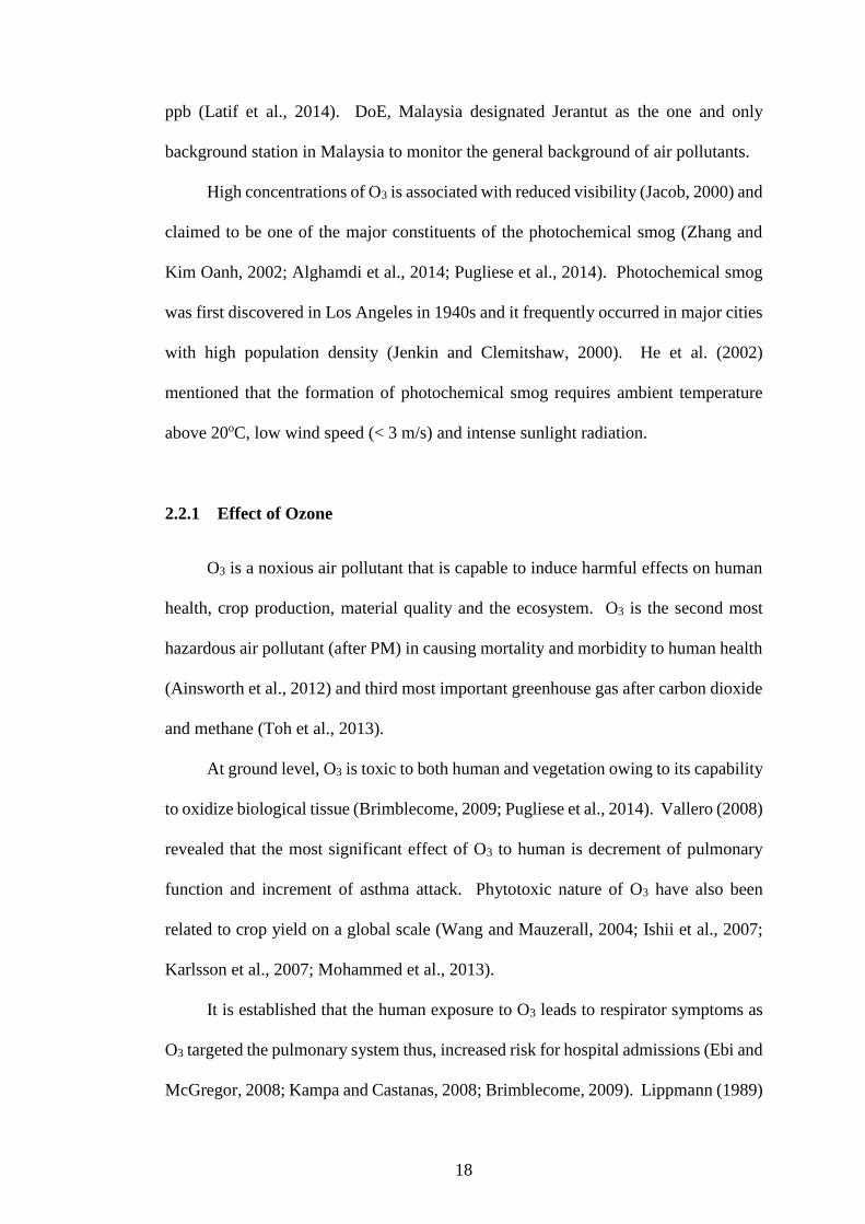
2.2.1 Effect of Ozone
O3 is a noxious air pollutant that is capable to induce harmful effects on human
health, crop production, material quality and the ecosystem. O3 is the second most
hazardous air pollutant (after PM) in causing mortality and morbidity to human health
(Ainsworth et al., 2012) and third most important greenhouse gas after carbon dioxide
and methane (Toh et al., 2013).
At ground level, O3 is toxic to both human and vegetation owing to its capability
to oxidize biological tissue (Brimblecome, 2009; Pugliese et al., 2014). Vallero (2008)
revealed that the most significant effect of O3 to human is decrement of pulmonary
function and increment of asthma attack. Phytotoxic nature of O3 have also been
related to crop yield on a global scale (Wang and Mauzerall, 2004; Ishii et al., 2007;
Karlsson et al., 2007; Mohammed et al., 2013).
It is established that the human exposure to O3 leads to respirator symptoms as
O3 targeted the pulmonary system thus, increased risk for hospital admissions (Ebi and
McGregor, 2008; Kampa and Castanas, 2008; Brimblecome, 2009). Lippmann (1989)

19
claimed that the only significant exposure route of O3 pollutant is through inhalation
and inhalable concentration that is assumed to be at par with ambient concentrations
recorded at monitoring stations. Once it is inhaled, the dose targeted the tissue in
respiratory system and the effect of O3 is intensified with more exercise as the
breathing flow rate is increasing (Lippmann, 1989). Pires et al. (2008b) specified the
concerning health effect from O3 are damage to respiratory tract tissue, death of lung
cells, inflammation of airways and increase in respiratory symptoms (cough, chest
soreness and difficulty in taking deep breath). According to Bernstein et al. (2004)
exposure to approximately 100 to 400 ppb of O3 concentrations can cause neurophilic
inflammations as early as an hour after the exposure and persisted up to 24 hours.
Various studies elucidated that the phytotoxic nature of O3 air pollutant is the
main criteria in affecting the plants (Ishii et al., 2007; Lindroth, 2010; Ainsworth et
al., 2012; Banan et al., 2013; Mohammed et al., 2013). O3 concentrations that were
higher than 40 ppb may induce negative responds in terms of crops yields, biomass
production, vitality and stress tolerance of the plants (Fuhrer et al., 1997). Ainsworth
et al. (2012) listed that the major damaging effect of O3 pollution towards plants
include photosynthetic carbon assimilation, stomata conductance and reduction in crop
yield. Normally plants show effect of O3 when there is a speckle of brown spots on
the flat areas of the plant’s leaf in between the vein (Tiwary and Colls, 2009). O3 is
also capable to induce faster reduction of leaf area during crop senescence (Alvim-
Ferraz et al., 2006; Kovač-Andrić et al., 2009).
In evaluating the O3 impact on vegetation, accumulative exposure over a
threshold value (AOTX) is introduced. European nations adopted AOT40 as the
threshold limit starting from 1996. However, Mohammed et al. (2013) suggested that
AOT50 index is more suitable to be implemented in Malaysia as currently there are no

20
guidelines limit designed against the effect of O3 towards plant in this country and due
to differences in the climate and amount of solar radiation.
Unlimited to biological entities, ground level O3 can also effect the non-organic
materials as well. Arif and Abdullah (2011) mentioned that some materials such as
elastomers, textiles fibres, dye and paints are susceptible to O3. Damage area usually
takes the form of cracking leading to brittleness resulting in the reduction of the
materials strengths and increased rate of wear (Lee et al., 1996). Studies have also
revealed that paint pigments faded severely when it is exposed to high O3
concentrations which that has been observed during Los Angeles photochemical smog
(Solomon et al., 1992). According to Salmon et al. (2000) paint pigments and dye
based on indigo family is more susceptible to O3 damage. Additionally, O3 is also
capable in damaging the photographic materials and books (Godish, 1997) as well
increase in corrosion of building material such as steel, zinc, copper, aluminium and
bronze (Pires et al., 2008b).
2.2.2 Ground Level Ozone Fluctuational Behaviour
Ground level O3 exhibited different fluctuation features compared to other
primary air pollutants such as NO, NO2, CO and CO2. O3 showed strong daily, weekly
and seasonal variations (Jenkin and Clemitshaw, 2000; Duenas et al., 2004; Khoder,
2009; Han et al., 2012; Hassan et al., 2013). Hassan et al. (2013) claimed that diurnal
variations are very important in understanding the different processes responsible for
O3 formation and destruction. O3 showed clear diurnal trends which is very similar to
solar radiation diurnal trends (Duenas et al., 2004). The O3 concentration is normally
low in the morning and gradually increase towards the afternoon (Ghazali et al., 2010;
Alghamdi et al., 2014). Diurnal variation in O3 shows a maximum concentration

21
around noon or early afternoon with the values gradually decreasing as evening
approaches (Ghosh et al., 2013). Table 2.1 presents the summary of diurnal O3
fluctuation in different locations. O3 showed similar uni-modal trends that reach peak
concentration around afternoon or early evening.
Table 2.1 Characteristics of O3 diurnal trends
Location Duration Diurnal
cycle
Peak
hour
References
Urban areas,
Malaysia
2006 uni-modal 1-2 p.m. Ghazali et al. (2010)
Klang Valley,
Malaysis
2004-2008 uni-modal 2-4 p.m. Latif et al. (2012)
Jerantut, Malaysia 2005-2009 uni-modal 3 p.m. Banan et al. (2013)
Malaga, Spain - uni-modal 3 p.m. Duenas et al (2004)
Rural, India 2010 uni-modal 1 p.m. Reddy et al. (2012)
Tianjian, China 2010 uni-modal 2 p.m. Han et al. (2011)
Jeddah, Saudi
Arabia
2012-2013 uni-modal 1 p.m. Alghamdi et al. (2014)
Cairo, Egypt 2004-2005 uni-modal 2 p.m. Khoder (2009)
Generally, O3 concentration is higher during daytime as compared to nighttime
because photochemical reactions only occurs during daytime (Ghazali et al., 2010;
Reddy et al., 2011; Alghamdi et al., 2014). At night, O3 concentration is constantly
low primarily accounted for the absence of any photochemical production and further
destruction by continuous chemical loss by NO titration and deposition (Ghosh et al.,
2013). Considering the significant differences of O3 concentrations between daytime
and nighttime, several studies (Lengyel et al., 2004; Abdul-Wahab et al., 2005; Özbay
et al., 2011) stressed that there are O3 advantages of separating daytime and nighttime
O3 analysis due to different influencing factors. Table 2.2 summarizes the difference
between daytime and nighttime of O3 concentrations in Egypt, India and China.
O3 also exhibited clear seasonal fluctuations with the highest and lowest O3
concentrations observed during summer and winter seasons, respectively (Duenas et

22
al., 2004; Hassan et al., 2013; Iqbal et al., 2014). However, Md Yusof et al. (2010)
alleged that seasonal variations in Malaysia that experience the tropical rainforest
climate is different from the temperate countries that show four distinctive seasons
every year. In Malaysia monsoonal changes showed more prominent effects to O3
fluctuations (Ghazali et al., 2010; Latif et al., 2012) due to changes in the wind’s flow
pattern and rainfall intensity. Due to the difference in weather condition, Banan et al.
(2013) claimed that monthly variations of O3 in urban and sub-urban areas in Malaysia
are strongly dependent on wind pattern.
Table 2.2 Review of daytime and nighttime O3 concentrations
Location Duration Mean O3 (ppb) References
Daytime Nighttime
Cairo Egypt 2004-2005 64.70 27.50 Khoder, 2009
Kolkata India 2010-2011 26.00 9.00 Ghosh et al., 2013
Tieta China 2009 46.50 18.36 Han et al., 2012
Han et al., 2012 Wuqing China 2009 65.91 18.08
Anantapur India 2009 51.74 35.52 Reddy et al., 2011
Xi’an China 2009 23.64 7.10 Reddy et al., 2011
2.2.3 Ground Level Ozone Transformational Behaviour
There are no significant anthropogenic emissions of O3. The majority of ground
level O3 comes from photochemical reactions of methane, VOCs and NOx, which are
largely from anthropogenic emissions with the presence of sunlight (Ghazali et al.,
2010). It is expected that a minor component (approximately 10%) of tropospheric O3
are injected from stratospheric influx (Ainsworth et al., 2012), however the process is
still unclear.
O3 formation is influenced by the chemistry of its precursors, topography, type
of terrain, vegetation and meteorological conditions (Kovác-Andrić et al., 2009).
According to Alghamdi et al. (2014), some cases of O3 formations are entirely
controlled by NOx concentrations (NOx-sensitive), while in other cases, it is totally

23
dependent on VOC concentrations (VOC-sensitive). Zhang and Kim Oanh (2002)
added that the complexity of O3 formation and destruction is also contributed by the
involvement of physical and chemical processes in the lower troposphere and
exchange air with stratosphere. As a result, O3 is becoming the major pollutants that
can induce serious environmental problems and yet their transformation behaviour is
difficult to control and predict due to the effect of its precursors and meteorological
changes (Abdul-Wahab et al., 2005; Pires et al., 2008b; Özbay et al., 2011).
2.2.3 (a) Daytime Chemistry of Ground Level Ozone Transformation
O3 chemistry is much driven by the presence of sunlight as the pollutant itself
is normally called a secondary pollutant (Jenkin and Clemitshaw, 2000). The sunlight
initiated the photochemical reactions by providing near ultra violet radiation, which
dissociates certain stable molecules into the formation of free radicals. Atkinson and
Arey (2003), elucidated that the only significant formation route of O3 in the
troposphere began with photolysis of NO2 (2.2).
2 3O + O + M O + M (2.1)
2NO + hv ( < 400 nm) NO + O (2.2)
3 2 2NO + O NO + O (2.3)
Where M is a third element, such as N2 or O2, which removes energy of the reaction
and stabilizes the O3 (Teixeira et al., 2009). The reactions in equations (2.1), (2.2),
and (2.3) result in a photo-equilibrium between O3, NO2 and NO with no net
formations and loss of O3 (Atkinson, 2000; Nishanth et al., 2014). Jenkin and
Clemitshaw (2000) expressed that in a typical boundary layer concentration of 30 ppb
of O3, the O3 destruction reactions (2.3) occur on a timescale of around one minute.
During daytime, the chemical inter-converting the NOx species involving the free

24
radicals either hydroperoxy radical (HO2) or organic peroxy radicals (RO2) is
responsible in increasing the O3 concentration. These free radicals are mainly
produced in the troposphere as intermediates in the photochemical oxidation of carbon
monoxide (CO) and volatile organic compounds (VOCs) (Jenkin and Clemitshaw,
2000; Atkinson and Arey, 2003). Both HO2 and RO2 are capable in providing
additional NO2 concentration in the atmosphere through reactions (2.4) and (2.5).
2 2HO + NO OH + NO (2.4)
2 2RO + NO OH + NO (2.5)
Where HO2 is the hydroperoxy radical; OH is hydroxyl; RO2 is organic peroxy
radicals.
The additional NO2 concentration will directly be converted into O3 through
reactions (2.2) and subsequently cycled to produce additional NO and NO2
concentration. The production of NO2 through the reactions in (2.4) and (2.5) does
not consume O3, subsequently together with reaction (2.1) and (2.2) represent the net
source of O3 at ground level (Atkinson, 2000; Jenkin and Clemitshaw, 2000; Seinfeld
and Pandis, 2006; Tiwary and Colls, 2009).
Additional O3 concentrations are also contributed by the CO concentrations.
Reaction with OH oxidized CO into CO2 through reactions (2.6) and generates HO2
through (2.7). The chemical reaction between HO2 and NO then take place to produce
NO2 (2.4), which is later converted into O3 (Jacob, 2000).
2OH + CO H + CO (2.6)
2 2H + O + M HO + M (2.7)
Where H is hydrogen atom; M is a third molecule (N2 or O2).
Nishanth et al. (2014) stated that the loss of O3 concentration during daytime
is mainly attributed by scavenge by NO titration (2.3) and their photolysis into O atom