Embed Size (px)
Citation preview
Faculty of Environmental Sciences
Assessment of Impacts of Changes in Land Use Patterns
on Land Degradation/Desertification in the Semi- arid
Zone of White Nile State, Sudan, by Means of Remote
Sensing and GIS
This thesis is submitted to fulfill the partial requirements for degree of Doctor of
Natural Science (Dr.rer.nat)
Submitted by
MSc. Abdelnasir Ibrahim Ali Hano, born on 01.10.1971, in Elginina
Supervisor:
Prof. Elmar Csaplovics, Institute of Photogrammetry and Remote Sensing, TUD.
Prof. Mubark Abdelrahman, Institute of Desertification and Desert Cultivation
Studies, U of K, Sudan
PD Dr. Hannelore Kusserow, Department of Earth Sciences, FU Berlin.
Dresden, 2013
II
Explanation of the doctoral candidate
This is to certify that this copy is fully congruent with the original copy of the thesis
with the topic:
Assessment of Impacts of Changes in Land Use Patterns on Land
Degradation/Desertification in the Semi- arid Zone of White Nile State,
Sudan, by Means of Remote Sensing and GIS
.
Dresden, Germany, 11.10. 2013 ……………………………………….…. Place, Date Ibrahim Ali Hano, Abdelnasir ……………………………………….…. Signature (surname, first name)
III
Declaration
I hereby declare that this thesis entitled ′′Assessment of Impacts of Changes in
Land Use Patterns on Land Degradation/Desertification in the Semi- arid
Zone of White Nile State, Sudan, by Means of Remote Sensing and GIS′′
Submitted to the faculty of environmental science Technical University of Dresden
(TUD), is my own work and, it contains no material previously published or written
by another person, nor material which to a substantial extent has been accepted
for the award of any other degree or diploma of the university or other institute of
higher learning, except where due acknowledgement has been made in the text.
Necessary contacts to the officials and private individuals and the use of image
processing facilities have been done as mentioned in this thesis and with the
agreement of the supervisors.
Abdelnasir Ibrahim Ali Hano
Dresden, Germany
October, 2013

IV
Dedication
To the soul of my father (Ibrahim), brother (Osam), sister (Saadia) and father in low (Khalid Omer), who, were died during my PhD research period.
To my small family (my wife (Marwa) and my children (Manarra, Mohammed,
Ahmed and Ibrahim)).
To my big family (my mother (Khadeeja) and my brothers and sisters)
V
TABLE OF CONTENTS
TABLE OF CONTENTS ......................................................................................... V
LIST OF TABLES ................................................................................................... X
LIST OF FIGURES ............................................................................................... XI
LIST OF APPENDICES ...................................................................................... XV
LIST OF ACRONYMS ........................................................................................ XVI
ACKNOWLEDGMENT ....................................................................................... XIX
ABSTRACT ........................................................................................................ XXI
ZUSAMMENFASSUNG ................................................................................... XXIII
Chapter One
Study Themes, Aims, and Objectives ................................................................ 1
1.1 Background .................................................................................................... 1
1.2 Problem statement and justifications ............................................................. 5
1.3 Aims and objectives ....................................................................................... 6
1.4 The study hypotheses .................................................................................... 7
1.5 Study area and Methodology ......................................................................... 8
1.5.1 Study area and its importance .................................................................... 8
1.5.2 Methodology ............................................................................................... 9
1.6 Outline and methods of the thesis ................................................................ 10
Chapter Two
Review of Land Degradation & Desertification and Influence of Land Use
Patterns Change ................................................................................................ 12
2.1 Arid and semi-arid lands ............................................................................... 12
2.2 Land degradation & desertification (LDD) .................................................... 12
2.2.1 Definitions, terms, and concepts ............................................................... 13
2.2.2 Causative factors of the LDD .................................................................... 15
VI
2.2.2.1 Causative factors of vegetation and soil degradation .............. 16
2.2.3 Indicators of LDD (vegetation and soil) ..................................................... 17
2.2.4 Methods for LDD assessment ................................................................... 18
2.3 Arid and semi arid land in Sudan ................................................................. 19
2.4 LDD in Sudan ............................................................................................... 19
2.4.1 Status and assessment of LDD ................................................................. 19
2.4.2 Causative factors of LDD in Sudan ........................................................... 22
2.4.3 Status and causative factors of vegetation and soil degradation .............. 23
2.4.4 Biophysical and socioeconomic indicators of LDD in Sudan ..................... 24
2.5 Effects of the LUC on LDD ........................................................................... 24
2.5.1 In general .................................................................................................... 24
2.5.2 Effects of LUC on LDD in Sudan ............................................................... 25
Chapter Three
RS and GIS Applications in Land Use and Land Degradation/Desertification
............................................................................................................................. 33
3.1 Background .................................................................................................. 33
3.1.1 Remote sensing ........................................................................................ 33
3.1.2 Integration of RS and GIS ......................................................................... 34
3.2 Applications of RS and GIS in land use change and land degradation in
dryland ................................................................................................................. 35
3.3 RS and GIS for mapping and obtaining information of LU and LDD ............ 36
3.3.1 Image classification ................................................................................... 37
3.3.1.1 Vegetation and soil indices for LDD assessment ................................... 37
3.3.1.2 Pixel-Based Image Analysis (PBIA) ....................................................... 40
3.3.1.3 Object Based Image Analysis (OBIA) .................................................. 43
3.3.2 Determination of spatiotemporal rate and trend of LU and LDD .............. 45
VII
3.3.3 A fusion of RS and ancillary data set for correlating and modelling the LUC
and LDD ............................................................................................................... 46
Chapter Four
Description of Study Area and Methodology .................................................. 48
4.1 Description of Study area ............................................................................. 48
4.1.1 The Sudan ................................................................................................ 48
4.1.1.1 Location ................................................................................................. 48
4.1.1.2 Climate and vegetation cover ................................................................. 49
4.1.2 White Nile State ........................................................................................ 49
4.1.2.1 Climate ................................................................................................... 50
4.1.2.2 Soils ....................................................................................................... 51
4.1.2.3 Vegetative Cover.................................................................................... 51
4.1.2.4 Desertification and drought in the White Nile State ................................ 52
4.1.3 Elgeteina Locality (study area) ............................................................... 52
4.1.3.1 Administrative Units ............................................................................... 54
4.1.3.2 Population distribution ............................................................................ 54
4.1.3.3 Human activities and LU ........................................................................ 55
4.1.3.4 Desertification and LD ............................................................................ 56
4.2 Methodology ................................................................................................ 58
4.2.1 Data selection and collection .................................................................... 58
4.2.2 Image preprocessing and enhancement ................................................... 62
4.2.3 Approaches of image processing for deriving information ......................... 63
4.2.3.1 Visual image interpretation ..................................................................... 63
4.2.3.2 The biophysical indices approach: ......................................................... 63
4.2.3.3 Pixel based- and object-based image analysis approach ..................... 67
4.2.3.3.1 Pixel based image analysis ................................................................. 67
VIII
4.2.3.3.1.1 Hybrid classification ......................................................................... 67
4.2.3.3.2 Object-based image analysis……………………………………………..69
4.2.3.3.3 Assessment of classification performance .......................................... 74
4.2.3.4 Change detection and matrix to estimate the changes in land use and
land degradation .................................................................................................. 74
4.2.3.5 A fusion of climatic, socioeconomic and remote sensing data approach 75
Chapter Five
Findings of Analysis of Multi Temporal and Spectral Imagery and Ancillary
Datasets for the LDD and LU Patterns in a Semiarid Area of Elgeteina ........ 76
5.1 Assessment of LDD by using biophysical indices ........................................ 76
5.1.1 Assessment of vegetation degradation by using appropriate vegetation
indices .................................................................................................................. 76
5.1.2 Assessment of the soil degradation status by using GSI .......................... 83
5.2 Assessment of LU and LDD by using pixel based- and object-based
approaches .......................................................................................................... 87
5.2.1 A more appropriate approach for LU and LDD assessment ...................... 87
5.2.2 Analysis of effects of LUC on LDD by using OBIA .................................... 90
5.3 Modelling the influence of LUC on LD ..................................................... 100
5.3.1 Model building of LU patterns affecting LDD ........................................ 100
5.3.1.1 Modelling the LU classes (patterns) change affecting vegetation cover
degradation .......................................................................................................... 99
5.3.1.2 Modelling the LU patterns change affecting soil degradation ............. 103
5.4 Analysis of proposed causing factors of LUC and/ or LDD in the study area
........................................................................................................................... 106
5.4.1 Impact of climate variability on LUC and/or LDD dynamic .................... 106
5.4.2 Indirect human inducing factors of LU patterns change and/or LDD ....... 109
IX
Chapter Six
Discussion ........................................................................................................ 114
6.1 Assessment of LDD ..................................................................................... 114
6.2. Assessment of LUC impact on LDD by using PBIA and OBIA approach .. 116
1) Comparison between PBIA and OBIA, for assessing LU and LDD .............. 116
2) Spatiotemporal trend of the LU Classes (patterns) and LDD in the periods
1973–1986 and 1986–2009: .............................................................................. 116
3) Effects of LU patterns change on LD: ........................................................ 116
3) Modelling the influence of LU patterns change on LD ................................ 118
4) Driven factors of LU change and/or LDD and LDD in the study area: ............ 118
Chapter Seven
Conclusions, Recommendations, and Outlook ............................................. 118
Conclusions ....................................................................................................... 118
Constraints ......................................................................................................... 119
Recommendation ............................................................................................... 119
Outlook .............................................................................................................. 120
Literature Cited ................................................................................................ 121
Appendices ....................................................................................................... 155
X
LIST OF TABLES
Table (2.1). Agricultural cultivated area in 2003/04 and 2005/05 season in
Sudan (Million feddans) ....................................................................................... 29
Table (2.2). Land area under different LU categories in Sudan (million ha: Elsiddig
et al., 2004) .......................................................................................................... 30
Table (3.3). Definition and calculation of some vegetation indices ....................... 40
Table (4.1). Administrative units and village numbers (Source: Central Bureau of
Statistics of the State (2009)) ............................................................................... 54
Table (4.2). Population distribution in administrative units (Source: Central Bureau
of Statistics of the State (2009)) ........................................................................... 54
Table (4.3). Land use and land cover categories (Source: FAO (2012)) .............. 55
Table (4.4). The database used for the study ...................................................... 60
Table (4.5). The characteristics of the selected database used in the research .. 61
Table (4.6), the characteristics of vegetation and soil indexes used in the research
............................................................................................................................. 64
Table (4.7). Segmentation parameters ................................................................ 71
Table (4.8): Feature categories used for separatability ........................................ 73
Table (4.9). Threshold values of LU/LD ............................................................... 73
Table (5.1). Comparison between different vegetation indices in articulating the
different types of vegetation covers in semiarid zone .......................................... 79
Table (5.2). Accuracy assessment of classification (PBIA) – hyper classification –
MLC ..................................................................................................................... 89
Table (5.3). Accuracy assessment of classification (OBIA) – fuzzy logic classifier
............................................................................................................................. 90
Table (5.4). Areas of LU/LC patterns and LD and the change trend of LU/LC and
LD from 1973–1986 and 1986–2009 (area in Km2)……………………………….. 92
XI
Table (5.5). Pearson matrix correlation between LU/LCC from 1973–2009 (Author,
2012) .................................................................................................................. 101
Table (5.6) Coefficientsa ..................................................................................... 100
Table (5.7). Coefficients ..................................................................................... 104
Table (5.8). Pearson correlation climate variation and LUC 1973–2009 (The
author, 2012) ...................................................................................................... 108
Table (5.9). Climate variability correlation with LD and land cover during 1973–
2009 (The author, 2012) .................................................................................... 109
Table (5.10). Coefficient correlation of population growth rate and LU/LCC and LD
(The author, 2012) ............................................................................................. 110
XII
LIST OF FIGURES
Figure (1.1). Hypothesized flow chart of causing factors of LUC and/or LDD ........ 8
Figure (2.1). The distinction between land degradation, desertification and soil
degradation (Source: Akhtar (2009)) .................................................................... 15
Figure (2.2). Global causes of LDD process (Lal et al., 1989). ............................ 16
Figure (2.3). Map and percentage of Sudan land cover (Source: FAO (2012)). .. 27
Figure (2.4). Livestock population estimations of Sudan from 1990–2008 (in
millions) (Source: Animal Wealth Ministry (2008)) ............................................... 28
Figure (4.1). Map of Sudan developed by the Author (2011) ............................... 49
Figure (4.3). Map of White Nile State developed by the Author (2011) ................ 50
Figure (4.4). Map of study area (Elgeteina Locality) developed by the Author
(2011) .................................................................................................................. 53
Figure (4.5). Rate of rainfall in the study area (Source: Sudan’s General Authority
of Meteorology 2008..............................................................................................53
Figure (4.6). LU/LC of the locality (Source: FAO (2012))......................................55
Figure (4.7). Animal population of the locality (Source: Central Bureau of Statistics
of the State (2009)) .............................................................................................. 56
Figure (4.8). Some of the LDD status in 2010, photographs by the Author (2009)
............................................................................................................................. 57
Figure (4.9). Flow diagram of the image analysis ................................................ 59
Figure (4.10). Scenes and subsets of study area (Elgetiena locality) ................. 62
Figure (4.11). Flow diagram of hybrid classification processing ........................... 68
Figure (4.12). Flow diagram of OBIA process ...................................................... 70
Figure (4.13). Hierarchical network of segments produced by multi-resolution
segmentation ....................................................................................................... 72
Figure (5.1). Maps of vegetation indices .............................................................. 78
XIII
Figure (5.3). Map and areas of vegetation degradation grades ........................... 81
Figure (5.4). Maps of the spatiotemporal trend of vegetation degradation ........... 82
Figure (5.5) shows the spatiotemporal trend vegetation
degradation………………………………………………………………………………82
Figure (5.6). GSI map (1) and soil distribution and sand dunes map (2) .............. 84
Figure (5.7), mapping and measurement of the soil degradation area ................. 85
Figure (5.8). Maps of spatiotemporal trend of soil degradation ............................ 86
Figure (5.9). Spatiotemporal trend of soil degradation ......................................... 86
Figure (5.10). Maps of LU/LDD by using PBIA and OBIA .................................... 88
Figure (5.11). Thematic maps of LU/LD for 1973, 1986, and 2009 ...................... 93
Figure (5.12). Increase and decrease trends of LU/LD. ....................................... 94
Figure (5.13). The LU change effects on the vegetation degradation from 1973–
1986 ..................................................................................................................... 96
Figure (5.14). The LU change effects on the vegetation degradation in 1973–1986
and from 1986–2009 ............................................................................................ 97
Figure (5.15). LU and SDL (moved sand dunes) dynamic from 1973–1986 ........ 98
Figure (5.16).LU and SDL (moved sand dunes) dynamic from 1986–2009 ......... 99
Figure (5.17). Histogram of checking the assumption of normal distribution of the
error ................................................................................................................... 103
Figure (5.18). Normal P-P plot of regression standardized residual (error) ........ 103
Figure (5.19). Histogram for checking the assumption of the normal distribution of
the error ............................................................................................................. 105
Figure (5.20). Normal P-P plot of the standardized residual of the regression
(error) ................................................................................................................. 105
Figure (5.21). Linear regression of average annual rainfall of the Khartoum and
Eldweim stations ................................................................................................ 107
Figure (5.22). Status of RH, MT, and WS from 1973–2009 ............................... 107
XIV
Figure (5.23). The main jobs of the local population (Author, 2012 .................... 110
Figure (5.24). The local people’s practices and their relation to LUC and LD (The
author, 2012) ...................................................................................................... 111
Figure (5.25). The different patterns of agricultural practices (Author, 2010) ..... 111
Figure (5.26). The different energies used by local people for cooking (Author,
2012). ................................................................................................................. 112
Figure (5.27). The products local people used to build their houses (Author, 2012).
........................................................................................................................... 112
Figure (5.28). Different land tenure systems in the study area (Author 2012) ... 113
XV
LIST OF APPENDICES
Appendix (1) set of the analysis software was used in the study ....................... 155
Appendix (2). Questionnaire .............................................................................. 156
Appendix (3), LU/LD change matrix in 1973 – 1986 (area in Km2) .................. 158
Appendix (4), LU/LD matrix change in 1986 to 2009 (area in Km) ................... 158
Appendix (5), map of LU change effects on the vegetation degradation in 73 -
1986 ................................................................................................................... 159
Appendix (6), map of LU patterns and vegetation dynamic of 1986 – 2009 ..... 159
Appendix (7), map of LU/LC and sand dunes dynamic in 73 - 1986 ................ 161
Appendix (8), map of LU/LC and sand dunes dynamic of 1986 - 2009 ........... 161
Appendix (9), mutual conversion between LC patterns and DWL 73 - 1986 ...... 162
Appendix (10), mutual conversion between LC and MRL 73 - 1986 ................ 163
Appendix (11), mutual conversion between LC patterns and DWL 86 -2009 ..... 164
Appendix (12), mutual conversion between LC patterns and MRL 86 -2009 ..... 164
Appendix (13), mutual conversion between LC patterns and SDL 73 -1986 ...... 165
Appendix (14), mutual conversion between LC patterns and MRL 86 -2009 ..... 165
Appendix (15) data set of LU/LC, Climate, population growth rate for model and
correlation .......................................................................................................... 166
Appendix (16). Model summary ......................................................................... 167
Appendix (17). Analysis of variance ................................................................... 167
Appendix (18). Residuals Statistics .................................................................... 168
Appendix (19). Model summary ......................................................................... 168
Appendix (20). Analysis of variance ................................................................... 168
Appendix (21). Residuals Statistics.....................................................................168
XVI
LIST OF ACRONYMS ASSOD Soil Degradation in South and Southeast Asia
ASTER Advanced Space borne Thermal Emission and Reflection
DECARP Desert Encroachment Control and Rehabilitation Program
D-JAM Darfur Joint Assessment Mission
DSD Dryland Science for Development Consortium
ERDAS Earth Resources Data Analysis System ETM+ Enhanced Thematic Mapper plus
FAO Food and Agriculture Organization
FLAASH Fast Line-of-sight- Atmospheric Analysis of Spectral
Hypercubes
GCPs Ground Control Points
GDP Gross Domestic Products
GEOBIA Geospatial Object-Based Image Analysis
GIS Geographical Information System
GLASOD Global Assessment of Soil Degradation
GLCF Global Land Cover Facility
GPS Global Positioning System
IRS-1 Indian Remote Sensing-1
ISRIC International Soil Reference and Information Centre.
IUCN International Union for Conservation of Nature
Kg Kilogram
Km2 Square Kilometer
LADA Land Degradation Assessment
LDD Land Degradation and Desertification
LUC Land Use Change
LULC Land Use Land Cover
MEA Millennium Ecosystem Assessment
MIR Mid Infrared
MLC Maximum Likelihood Classifier
MODIS Moderate Resolution Imaging Spectroradiometer
MSS Multispectral Scanner
XVII
ND4-25 Normalized difference band 4-band 2 and 5
ND42-57 Normalized difference band 4 and -band 2- band5 and7
NDDCU National Drought and Desertification Control Unit
NDVI Normalized Difference Vegetation Index
NIR Near Infrared
OBIA Object-Based Image Analysis
Radiometer
RMSE Root Mean Square Error
RS Remote Sensing
SARVI Soil Adjusted and Atmospheric Resistant Vegetation Index
SAVI Soil Adjusted Vegetation Index
SAVI Soil Adjusted Vegetation Index
SI Soil Index SIFSIA-N Sudan Institution Capacity Programme: Food Security
Information
SPOT System Pour 1´Óbservation de la Terre
SWIR Short Wave Infrared
TIR Thermal infrared
TM Thematic Mapper
UN United nation
UNCED United Nation Conference on Environmental Development
UNCOD United nation Conference on Desertification
UNDESA United Nations Department of Economic and Social Affairs
UNEP United Nations Environment Program
UNESCO United Nations Educational, Scientific and Cultural
Organization
UTM Universal Transverse Mercator Projection
UV Ultraviolet
VI Vegetation Index
VNIR Visible and Near Infrared
WHO World Health Organization
WMO World Meteorological Organization
XVIII
WRS World Reference system
XIX
ACKNOWLEDGMENT
First of all, I am grateful to the Almighty God (Allah) for establishing me to
complete this PhD research. It is with immense gratitude that I acknowledge the
support and help of my supervisor, Prof. Dr Elmar Csaplovis, the head of the
remote sensing chair, TUD and for his acquaintances, fruitful, wonderful
supervision as well as for his fine ethics.
My deepest thank extends to the Dresden university administration, particularly
remote sensing department for giving me acceptance and providing me with
essential PhD requirements; especially thank extends to my colleagues Stephan
Schoeps, Christine Wessolk and Yan Schmits
A lot of Thanks to Ministry of High Education, particularly the training
administration (Sudan) for full financial support to my study and to Khartoum
university administration, particularly the teaching assistant administration for the
assistance and follow up during my study.
I am gratefully indebted to the German Exchange Academic Program (DAAD) and
Gesell Schaft Von Freunden und Fordern der (GFF) for partial support which
contributed or pushed me forward to rearch to the end of my study.
My thanks extend to Faculty of forestry especially to: Abdel Allah Mirgany the
dean of faculty of Forestry who supported me with transport for field survey and
Omer Said the head of forest conservation and protection department who
engaged me to do the PhD in Germany. Especially thank extends to Galal Elawad
a lecturer in the same department, Eltayeb Hamid a lecturer in the forest
management department , Faisal Ahmed Yaseen and Jameel Gumma are lab
techniques and Mortada the car driver who travelled with me and assisted me in
achieving the field and social survey perfectly.
I would like also to thank the:
• Forest national corporation and Elgeteina forest corporation (Hawa elnaby,
Khalid Kamal, Mustafa Osman and the people of Elgeteina who aided me
in performing my field work, easily.
• Elgeteina Locality staff who gave me valuable information regarding status
of population of Elgeteina.

XX
• My colleagues inside and outside University of Dresden particularly the
Sudanese colleagues and their families
I owe my deepest gratitude to my small family: to my wife Marwa Khalid and my
children: Manara, Mohammed, Ahmed and Ibrahim and to my big family, who
supported me materially and morally. Moreover my deepest thank and
appreciation to the family of my wife who gave full care to my children during my
absence.
XXI
ABSTRACT In Sudan, land degradation/desertification (LDD) has devastated large areas and
consequently, it includes social, economic, and environmental aspects. LDD
results from various factors, including climatic variation and human activities.
Probably the LU practices and their changes have contributed to an increase of
LDD in that area. Remote sensing technology has become unique and developed
tool for providing temporal and spatial information for the LDD research and other
environmental aspects. Determination of LDD and its relationship to land use
pattern change (LUC) at spatiotemporal scale is rare, critical issue, and is one of
the recommended research in semi-arid regions of Sudan. The study was carried
out to derive accurate and improved spatiotemporal information: to assess the
status of land LDD of vegetation and soil, to assess and model influences of the
LUC on LDD, and moreover to analyse the synergistic factors that have caused
the land use change and/or LDD in semi- arid zone of Elgeteina Locality in While
Nile State, Sudan during the last 36 years, using appropriate remote sensing (RS)
and GIS technology.
The study used four-cloud free images of different sensors (MSS 1973, TM 1986,
ASTER 2009 and TM 2010). The imageries were Geo-referenced and
radiometrically corrected by using ENVI-FLAASH software. Then subsets of the
study area were taken, ranging from 1600-2000 Km2. The study applied the new
approach of integration between vegetation and soil indices and in situ data to
assess the LDD. Comparison between pixel based image analysis (PBIA) and
latterly approach of object based image analysis (OBIA) was done by selecting
the best one for mapping LUC and LDD accurately. The change detection - matrix
was applied to estimate the spatiotemporal of changes in land use and land
degradation. Moreover, correlation and model approach was employed for fusing
the climatic, socioeconomic and remote sensing data to determine the
relationships between the different factors and to analyse the reasons for the LUC
and LDD as well as for modelling LU effects on LDD.
The study revealed that: The changes in land use patterns (RA, FWL and FML)
took place in 1973 – 86 – 2009, and affecting thoroughly different patterns of the
vegetation cover. Likewise the LUC affected soil degradation which led to the
XXII
movement of sand dunes in 1973 – 2009. The agricultural activity is the dominant
and has more effect on LDD particularly on the vegetation cover degradation. The
population growth and the socioeconomic status of local people are the main
indirect human inducing factors responsible for LUC and/or LDD. SARVI is slightly
more efficient than NDVI, SAVI, ND4-25 and ND42-57, for detecting the
vegetation status in semi-arid area, therefore the study selected it for the
assessment. GSI proved highly efficient in determining the different types of soil
degradation, and in producing the map of top soil grain size, which assisted in the
assessment of land degradation and desertification. OBIA-fuzzy logic
classification performed better than the PBIA- hybrid classification for assessing
LU patterns impact on LDD.
The study recommends to: replication of this study by using different imagery with
high resolutions and sophisticated software, such as eCognition and Feature
Analyst (FA) for increasing the validity and accuracy of the assessment and
modelling of LU patterns and LDD status in dry land is important in the Sudan.
XXIII
ZUSAMMENFASSUNG Im Sudan hat Land Degradation / Desertifikation (LDD) weite Gegenden
verwüstet, wobei hierbei soziale, wirtschaftliche und Umweltaspekte eine Rolle
spielen. LDD wird von verschiedenen Faktoren ausgelöst, darunter
Klimavariationen und menschliche Aktivitäten. Wahrscheinlich haben
Landnutzungspraktiken und ihre Änderungen zu erhöhter LDD in der
untersuchten Gegend beigetragen. Fernerkundungstechnologien sind sehr gute
und weit entwickelte Werkzeuge um zeitliche und räumliche Informationen zur
Erforschung von LDD und anderen Umweltaspekten zu ermitteln. Die
Bestimmung von LDD und ihre Beziehung zur Änderung von
Landnutzungsmustern (LUC) im raum-zeitlichen Maßstab ist bislang noch selten
erforscht und ist ein Forschungsbereich, der für die semi-ariden Regionen des
Sudan empfohlen wird. Die Studie wurde durchgeführt, um genaue und
verbesserte raum-zeitliche Informationen zu gewinnen: um den Status der LDD
von Vegetation und Boden zu bewerten, um den Einfluss des
Landnutzungswandels auf LDD zu beurteilen und zu analysieren, und außerdem
um die synergetischen Faktoren die den Landnutzungswandel und/oder LDD
verursacht haben zu analysieren. Dabei wurde die semi-ariden Zone des
Elgeteina Gebietes im Staat Weisser Nil (Sudan) während der vergangenen 36
Jahren unter Verwendung von geeigneter Fernerkundungs- und GIS-Technologie
untersucht.
Für die Studie wurden vier wolkenfreie Bilder von verschiedenen Sensoren (MSS
1973, TM 1986, ASTER 2009 and TM 2010) verwendet. Die Bilder wurden
georeferenziert und radiometrische korrigiert, wobei die ENVI-FLAASH Software
verwendet wurde. Anschließend wurden Teilgebiete des Untersuchungsgebietes
mit einer Größe zwischen 1.600 und 2.000 Km2 ausgewählt. In der Studie fand der
neue Ansatz der Integration von Vegetation und Boden Indizes und in-situ Daten
Verwendung, um LDD zu bewerten. Ein Vergleich von pixel-basierter Bildanalyse
(PBIA) und einem Ansatz von objekt-basierter Bildanalyse (OBIA) wurde
durchgeführt, um die beste Methode der Kartierung von LUC und LDD ermitteln.
Veränderungsmatrizen wurden eingesetzt, um räumlich-zeitlichen Änderungen
der Landnutzung und Land Degradation abzuschätzen. Außerdem wurde ein
XXIV
Korrelation- und Modellierungs-Ansatz eingesetzt, um die klimatischen,
sozioökonomischen und Fernerkundungsdaten zu verschmelzen und das
Verhältnis zwischen den unterschiedlichen Faktoren zu bestimmen und um die
Gründe für LUC und LDD zu analysieren aber auch um die Auswirkungen der
Landnutzung auf LDD zu modellieren.
Die Studie hat folgendes gezeigt: Die Änderungen der Landnutzungsmuster (RA,
FWL and FML) fand in 1973 – 86 – 2009 statt und betraf sehr unterschiedliche
Vegetationsmuster. Ebenso hatte die LUC Auswirkungen auf die
Bodendegradation, was zu einer Verschiebung von Sanddünen im Zeitraum 1973-
2009 führte. Landwirtschaft dominiert und hat starke Auswirkungen auf LDD,
insbesondere auf die Degradation der Vegetationsbedeckung. Die
Bevölkerungszunahme und der sozioökonomische Status der lokalen
Bevölkerung sind die wesentlichen indirekten menschlichen Faktoren die
verantwortlich für LUC und/oder LDD sind. SARVI ist etwas effizienter als NDVI,
SAVI, ND4-25 und ND42-57, um den Zustand der Vegetation in semi-ariden
Gebieten zu bestimmen, deshalb wurde dieser für die Studie ausgewählt. Es
stellte sich heraus, dass der GSI hoch-effizient war, sowohl bei der Bestimmung
der unterschiedlichen Typen von Bodendegradation als auch bei der Erstellung
von Karten der obersten Bodenkorngröße, die bei der Bewertung der
Landdegradation und Desertifikation half. OBIA-Fuzzy Logic Classification
arbeitete dabei etwas genauer und effizienter als die PBIA-Hybrid Classification,
um die Auswirkungen der Landnutzungsmuster auf LDD zu beurteilen.
Als Fortsetzung der durchgeführten Arbeiten empfiehlt sich eine nochmalige
Durchführung der Studie wobei anderes, hochaufgelöstes Bildmaterial und
anspruchsvolle Software, wie eCognition und Feature Analyst (FA) verwendet
werden sollten, um die Gültigkeit und Genauigkeit der Bewertungen und
Modellierung des LU und LDD Status von Trockenland im Sudan zu beurteilen.
Chapter One
Study Themes, Aims, and Objectives
This chapter is a gateway for this study, which includes three themes: land use,
land degradation and desertification (LDD), remote sensing (RS), and
geographical information system (GIS), and includes the aims, objectives, and
hypotheses of the study.
1.1 Background
“Land degradation” (LD) and in particular “desertification” are of global concern,
since they diminish the planet’s capacity to provide food to the world at large
(UNCCD, 2012). LD is defined as the ‘reduction or loss of the biological or
economic productivity and complexity of agricultural land (including rainfed
cropland, irrigated cropland, range, and pasture) forests and wood lands’ (United
Nations, 1994). Desertification has been given more than 100 definitions;
however, UNCCD (1994) offered the most recent and widely negotiated one: ‘land
degradation in arid, semi arid and dry sub humid areas, resulting from various
factors, including climatic variation and human activities.’ Desertification is the
label for LD in arid, semi-arid, and dry sub humid areas, collectively called dry
lands. Dry land areas cover more than 6.1 billion hectares of the earth’s surface.
LD is not limited to dry lands. Denti (2004) stated that it develops in many different
contexts: in cool dry and warm dry environments; in hugely arid and semi-arid
climates; on different types of soil and in very different societies in ancient and
modern advanced and traditional; rich and poor; capitalist and communist, and so
on. However, LDD is a much greater threat in drylands than in non-drylands
(Adeel et al., 2005). Grainger (1990) argued that LDD affects dry lands all over the
world, but tends to be concentrated in Asia and Africa, accounting for 37% of
desertified land. In some areas of the African Sahel, the surface area of the desert
is increasing rapidly. Purkis and Klemas (2011) stated that the annual southerly
march of the Sahara exceeds 40 km, engulfing vast tracks of arable land in its
path. There are diverse estimates of the extent of land degradation; five global
assessments over the last four decades have produced degradation estimates
2
ranging from 15% to 63% of global land and 4% to 74% of its subset of global
drylands (Safriel, 2007).
Desertification represents one of the most severe environmental hazards due to
the large amount of people and land at risk (Clarke and Noin, 1998). Although the
numbers vary, it is estimated that desertification directly affects one-third of the
earth’s land surface, affecting around 1.5 billion people, most of who live in
developing countries. An even higher number could be potentially affected (Clarke
and Nion, 1998; Murray, 1999; UNCCD, 2004a; Marini and Talbi, 2009). UNCCD
stated that approximately $42.45 billion of global income is lost annually due to
desertification (LEVIN Institute, 2012). Besides the immediate impact on people’s
livelihood, desertification is connected with other pressing global problems, as it is
accompanied by the loss of biological diversity and contributes to global climate
change through the loss of carbon sequestration capacity and an increase in land-
surface albedo (Röder and Hill, 2009). Most authors (e.g., Turner et al., 1995;
Puigdefábregas, 1998; Lambin et al., 2009) agree that no one single factor
causes LDD; it is caused by a combination of factors that change over time and
vary by location (MEA, 2005). The principal driver of human-caused LDD is
unsustainable exploitation of land productivity by pastoral, farming, and agro-
pastoral land uses (UNCCD, 2012).
The Sudan has become the third largest country (1,882,000 Km2) in Africa after
the secession of southern Sudan in July 2011 (Ministry of Information, 2011), and
it is affected seriously by desertification. Assessments show that severe and very
severe soil degradation covers a total area of 58 million hectares, while land
degradation totals 75 million hectares, indicating vegetation degradation of 17
million hectares (GLASOD, 1990; Dregne et al., 1991; Ayoub, 1998). The
degraded areas estimated above are situated in the northern states of the Sudan.
After separation of southern Sudan, division of the western states the affected
states have become 15 states out of 18 states. The most degraded zones are the
arid and semi-arid zones, where 76% of the human population lives (Mukhtar et
al., 2007).
3
In the Sudan, desertification is referred to as an outcome of both climate variants
(persistent drought) and human actions as excessive or unreasonable exploitation
of the environment. However, studies have stated, human action is the main
reason for desertification (Ayoub, 1997). The LDD phenomenon in Sudan was
reported by Kennedy-Cooke as early as in 1944 when rapid deterioration of soil
and vegetation occurred in parts of the Red Sea Hills. This was considered as a
warning sign that such problems might develop elsewhere, particularly around the
periphery of towns and settlements in Kordofan and the Darfur Provinces of
western Sudan.
LU/land cover change has important impacts on socioeconomic and
environmental systems with important tradeoffs for sustainability, food security,
biodiversity, and the vulnerability of people and ecosystems to global change
impacts (Lesschen et al., 2005). LU contributes widely to LD (Onur et al., 2009;
Ries, 2010). Many studies have revealed that LU changes and subsequent
conversion have led to a deterioration in the physical and chemical properties of
soil, causing degradation of the land (Braimoh and Vlek, 2004; Jiang et al., 2006;
Navarro et al., 2006; Khresat et al., 2008; Emadodin et al., 2009; Göl, 2009;
Korkanc et al., 2008; Li et al., 2009; Mahmoud et al., 2009; Zeng et al., 2009; Yao
et al., 2010). LU change refers to the complete replacement of one cover type by
another, for example deforestation or modification of certain type of LU (i.e.,
changes in the intensity of use or alterations of its characteristic
qualities/attributes) (Briassoulis, 2012). LU/LCCs are the result of the interplay
between socioeconomic, institutional, and environmental factors (Lesschen et al.,
2005). In tropical areas, LU practices that might have impacts on regional or even
global climate include large-scale clearing of rain forests, burning of biomass, bad
field cultivation, cattle breeding, and the subsequent overgrazing of semiarid
pasture grounds (Jacobeit, 1991).
LU and land cover in Sudan: the northern part of Sudan is mainly desert with few
agricultural areas concentrated along the rivers; in contrast, in the central part
(from eastern Darfur to Gedaref State), agricultural crops are the main cover
types. Agriculture is the main source of non-oil contributions to the GDP, ahead of
services and construction and much ahead of the industry. Recently, the FAO
4
(2012) did a land cover atlas of Sudan after separation of the Southern Sudan,
showing that the area of bare rocks and soil area is 50.7%, herbaceous area is
13.8%, agricultural area is 12.6 %, shrub area is 11.8%, and tree area is 10%.
Over the last decades, remote sensing (RS) has proven to be a valuable tool for
identifying objects at the earth’s surface and for measuring and monitoring the
spatiotemporal dimension of important biophysical characteristics and human
activities on the terrain (Steven and Freek, 2006). RS plays an important role in a
wide range of environmental disciplines, such as geography, geology, zoology,
agriculture, forestry, botany, meteorology, oceanography, and civil engineering.
Since the 1970s, thanks to its advantages in providing dynamical, multi-temporal
time series land cover information, RS has been applied widely in dry land
research, including assessment of LU changes and LD (Courel et al., 1984;
Tucker et al., 1986, 1991; Csaplovics, 1992; Graetz et al., 1988; Hellden, 1988,
1991; Hanan et al., 1991; Lambin and Strahler, 1994; Gao et al., 2001; Wu,
2003a-c and 2004; Wu et al., 2002 and 2005).
The integration of RS and GIS in environmental monitoring has become
increasingly common in recent years. RS imagery is an important data source for
environmental GIS applications, and conversely GIS capabilities are being used to
improve image analysis procedures (Hinton, 1996). An extended collaboration
between RS and GIS researchers has led to an increased cross-fertilization of
research ideas and information of new research agendas for both the GIS and RS
communities (e.g., Star, 1991; ASPRS, 1994; Legg, 1994; Sample et al., 1997).
Satellite RS is the only available means for systematic measurements of
spatiotemporal surface parameters over large areas in a reproducible manner and
at frequent rates. In fact, RS has long been recommended for its potential to
detect, map, and monitor degradation with high spatial and spectral resolution and
for the detection of degraded areas, including their dynamics of spread in time
(Sabins, 1987; Raina et al., 1993; De Jong 1994; Sommer et al., 1998; Sunjath et
al., 2000). Therefore, it can serve as a means for the monitoring of spatial and
temporal LD or LDD.
5
1.2 Problem statement and justifications
LDD has attracted wide concerns in recent years since hundreds of millions of
people in the world are affected and threatened by drought and famine, as well as
with the degradation of soils and vegetation (Paisley, Gaddis, and Greeley, 1991).
LDD is believed to be one of the most serious global environmental problems of
our time (Dregne et al., 1991; UNCED, 1992; Reynolds and Stafford Smith, 2002).
In Sudan, this phenomenon has devastated large areas and consequently, it
includes social, economic, and environmental aspects. As mentioned above, LDD
results from various factors, including climatic variation and human activities, but
likely human action is the main responsible factor. Studies have indicated that this
is the case in the Sudan by stating ‘high correlation seems to exist between
human population densities and degraded soil in different aridity zones’ (Ayoub,
1998). Considerably, LU is the most important impact among human activities and
affects the environmental balance and its influence on the land environment,
whether positively or negatively.
In White Nile State, signs of severe LD can be observed in different areas,
particularly in the Elgeteina area, the research area for this study. Probably the LU
practices and their changes contributed to an increase of LDD in that area.
Therefore, due to lack of studies and information in that important aspect, as well
as due to the recommendations of some workshops and Fora, particularly the
Forum for Proposing of a Plan of Action for Research on Desertification in Sudan:
White Nile State held in 2004 that directed researches towards focusing on the
temporal dimension of causative factors of LDD through assessment and
monitoring by using RS technology. RS has become a unique tool for fulfilling
several environmental studies and moreover, it is always developed and
advanced in all its system. Accordingly, the above factors led to the establishment
of this study, addressing the impacts of change in LU patterns on LDD at temporal
and spatial scales, by trading off efficient RS approach.
RS and GIS technology provide the most suitable and critical systematic
approaches for obtaining the spatial and temporal information so important in the
assessment of LDD and LU change accurately. In Sudan, assessments of LDD
and LU have become an important element in policy and decision making towards
6
sustainable LU management, consequently towards the environmental balance,
as well as contributing to the performance of “Zero Net Land Degradation – a
Sustainable Development Goal for Rio+20” held in 2012 (UNCCD, 2012).
Systematic long-term observations of LU/LCC are essential to enable scientists to
quantify the rates of change and their variability over time. The study can
contribute to a sound strategy and development plan for scientific research on
desertification and LU. Such research raises awareness at the local and national
level.
1.3 Aims and objectives
The overall aim of this study is to derive accurate and improved spatiotemporal
information, especially to assess and model influences of changes in the different
patterns of LU on LD by selecting appropriate approaches among traditional and
recent RS methods, integrating with GIS and some statistical analysis for 1973,
1986, 2009, and 2010. The objectives are as follows:-
• Assessment of the status of LDD of vegetation and soil based on
biophysical indicators, namely vegetation degradation and sand dune
formations and movement, by fusing RS (different vegetation and soil
indices) and GIS data, as well as situ data.
• Assessment of efficiency of vegetation indices (NDVI, SAVI, SARVI, ND4-
25, and ND42-57) and soil index (top soil surface grain size index (GSI)) in
determining and assessing LDD in semi-arid regions.
• Assessment of the spatiotemporal impact of the changes in LU patterns on
the vegetation degradation, based on comparison between PBIA, a hyper
classifier and OBIA, a fuzzy logic classifier, by supporting the in situ and
ancillary data.
• Assessment of the spatiotemporal impact of the changes in LU patterns on
soil degradation based on sand dunes formation and movement, based on
comparison between the PBIA classifier and the OBIA classifier, by
supporting the in situ and ancillary data.
• Mapping the changes in LU patterns and their effects on LDD.
7
• Modelling the impact of LU pattern changes on LDD based on vegetation
and soil degradation.
• Analysis of the synergistic factors that have caused the LU change,
consequently causing LDD.
1.4 The study hypotheses
• In the semi-arid zone, the situation of LDD trends is worsening rapidly with
an increase in soil and vegetation degradation.
• Analysis of the spatial and temporal dimension of LU patterns illustrate
rapid dynamics in LU patterns negatively affecting vegetation cover and
accelerating soil degradation in the semi-arid zone.
• Agricultural systems appear to affect LDD by the deteriorating vegetation
cover (deforestation), consequently causing soil degradation (formation and
movement of sand dunes), much more than other land use activities.
• Increase of soil degradation due to misuse of land consequently amplifies
sand accumulation and movement.
• SARVI is slightly better than NDVI, SAVI, ND4-25 and ND42-57 for
indicating vegetation cover in semi- arid regions.
• OBIA-fuzzy logic classification gives higher accuracy than PBIA-hybrid
classification in performing the assessment of LU pattern effects on LD.
• Different synergistic factors contribute to the changes of LU patterns or
LDD consequently; climatic variation and the growth of a population are
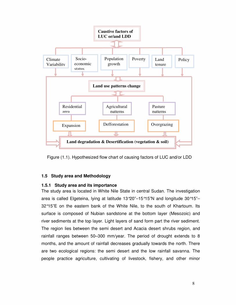
more significant driving factors (See Figure 1.1).
8
Figure (1.1). Hypothesized flow chart of causing factors of LUC and/or LDD
1.5 Study area and Methodology
1.5.1 Study area and its importance
The study area is located in White Nile State in central Sudan. The investigation
area is called Elgeteina, lying at latitude 13°20”–15°15”N and longitude 30°15”–
32°15”E on the eastern bank of the White Nile, to the south of Khartoum. Its
surface is composed of Nubian sandstone at the bottom layer (Mesozoic) and
river sediments at the top layer. Light layers of sand form part the river sediment.
The region lies between the semi desert and Acacia desert shrubs region, and
rainfall ranges between 50–300 mm/year. The period of drought extends to 8
months, and the amount of rainfall decreases gradually towards the north. There
are two ecological regions: the semi desert and the low rainfall savanna. The
people practice agriculture, cultivating of livestock, fishery, and other minor
Caustive factors of
LUC or/and LDD
Defforestation
Land
tenure
Poverty Socio-
economic
status
Population
growth Climate
Variability Policy
Land use patterns change
Overgrazing Expansion
Land degradation & Desertification (vegetation & soil)
Residential
area
Agricultural
patterns
Pasture
patterns
9
activities, such as trade, free works, and governmental jobs. The area of Elgeteina
was selected for this research study due to its importance among the localities of
the White Nile State. This locality is bordered by the capital of Sudan (Khartoum)
in the north and by the two important agricultural schemes El Gazera and El
Managel in the east. Also, there is a main road crossing that links the north with
western Sudan. The White Nile, one of the most important water bodies in Africa,
borders this locality. The appearance of desertification processes (wind erosion,
sand accumulation, and salinisation) in this region constitutes a serious threat on
the White Nile River.
1.5.2 Methodology
To achieve the aims and objectives of the research by applying means of RS and
GIS integrated with field survey and ancillary data, different approaches were
adopted and several steps were followed:
• Selection of satellite imagery data according to important considerations,
such as scale, spatial, temporal, and spectral resolutions of the sensors, as
well as atmospheric conditions and cost.
• Image pre-processing and enhancement.
• Integration of biophysical indices and in situ data to assess LD (vegetation
and soil): application of vegetation indices (NDVI, SAVI, SARVI, ND4-25,
and ND42-57) and soil index (GSI) for assessing LDD.
• Comparison between pixel based- and object-based image analysis for
mapping LU and LDD and for the different areas accurately.
• Post classification (change detection and matrix) to estimate the
spatiotemporal scale of changes in LU and LDD.
• Correlation and model approach: fusion of climatic, socioeconomic, and RS
data to find relationships between the different factors and to analyse the
reasons accounting for the LU pattern change and LD and for modelling LU
effects on LD.
10
1.6 Outline and methods of the thesis
The thesis consists of six chapters explicitly:
Chapter One (Study Themes and Aims and Objectives) provides background
information about LDD, problem statements and justifications, aims and
objectives, description of the study area and methodology, as well as the
hypotheses and outline and methods of the thesis.
Chapter Two (Review of Land Degradation & Desertification and Influence of
Land Use Patterns Change) reviews the definitions, causative factors, indicators,
and methods of assessing LDD generally, and reviews arid and semi-arid land,
the status and assessment, the causative factors, and the indicators of LDD in
Sudan specifically. Furthermore, it discusses the effects of changes of LU patterns
on LDD, as well as the driving factors of LU change or/and LDD in general, and
reviewing the effects of changes of the LU patterns on LDD in Sudan.
Chapter Three (RS and GIS Applications in Land Use and Land
Degradation/Desertification) tackles background information about RS and
integration of RS and GIS, applications of RS and GIS in the analysis of LU and
LDD, mapping and extracting information on LDD, and the LU change detection
matrix. Moreover, it reviews the integration of RS with ancillary data for correlating
and modelling the LU impact on LDD.
Chapter Four (Study Area and Methodology), contains the location description
and methodology. The location description includes socioeconomic, demographic,
and climatic characteristics of the study area. The methodology consists of data
selection and pre-processing and processing of imagery, as well as the analysis of
driving factors of LU change and/or LDD in the study area.
Chapter Five (Findings of Analysis of Multi Temporal and Spectral Imagery and
Ancillary Datasets for the Land Degradation and Land use in the semiarid region,
Elgeteina), reviews outputs of the methods of analysis taken for performing the
objectives. The results included the assessment of LDD by applying appropriate
indices, assessment of the impact of the changes in LU on LDD by comparing
between pixel- and object-based approaches, modelling, and predicting the
impact of LUC on LDD, as well as the analysis of driving factors of LU change
and/or LDD in the study area.
11
Chapter Six (Summary and Discussions) contains the summary and discussion of
critical results regarding the assessment of LDD, assessment of the impact of the
changes in LU patterns on LDD (vegetation and soil degradation), mapping the
impact of LU patterns on LDD, modelling the impact of LU patterns on LDD, and
analysis of some hypothesized driving factors of the changes in LU patterns
and/LDD.
Chapter Seven (Conclusions, Recommendations and Outlook) reviews the
conclusions about the application of RS technology, assessment of LDD and
assessing, mapping and modelling the impact of LU pattern changes on LDD, and
the analysis of the driving factors of LU pattern changes and/or LDD. The
recommendations concern critical points.
12
Chapter Two
Review of Land Degradation & Desertification and Influence of Land Use
Patterns Change
This chapter reviews the definitions, causative factors, indicators, and methods of
assessment of LDD generally, and reviews the status assessment, the causative
factors, and indicators of LDD in Sudan specifically. Furthermore, it discusses the
effects of changes of LU patterns on land LDD, as well as the driving factors of LU
change or/and LDD in general, and reviewing the effects of changes of the LU
patterns on LDD in Sudan.
2.1 Arid and semi-arid lands
Arid and semi-arid or subhumid zones (dry lands) are characterized by low erratic
rainfall of up to 700mm per annum, periodic droughts and different associations of
vegetative cover and soils. Interannual rainfall varies from 50-100% in the arid
zones of the world with averages of up to 350 mm. In the semi-arid zones,
interannual rainfall varies from 20-50% with averages of up to 700 mm. Regarding
livelihood systems, in general, light pastoral use is possible in arid areas and
rainfed agriculture is usually not possible. In the semi-arid areas, agricultural
harvests are likely to be irregular, although grazing is satisfactory (Goodin &
Northington, 1985). The majority of the population of arid and semi-arid lands
depends on agriculture and pastoralism for subsistence. Dry lands are fragile
environments are more subjective to LDD over the world, and are strongly
recognized areas of environmental research and policy development, focusing on
land use and land cover changes and particularly LDD.
2.2 Land degradation & desertification (LDD)
Desertification is the label for land degradation in arid, semi-arid, and dry sub
humid areas, collectively called dry lands. A significant portion of dry lands is
already degraded, and the ongoing desertification threatens the world’s poorest
populations and hinders the prospects of reducing poverty. Therefore,
desertification is one of the greatest environmental challenges today. It is a major
barrier to meeting basic human needs in dry lands and leads to losses in terms of
human well-being (greenfact.org, 2011).
13
2.2.1 Definitions, terms, and concepts
The origins of the word ‘desertification’ are most commonly attributed to
Aubreville’s (1949) work on tropical Africa forests (Davis, 2004). Etymologically,
the word desertification is derived from Latin. Desert has a twofold origin: (1) the
adjective desertus, that means uninhabited, and (2) the noun desertum, that
means a desert area; and on the other hand, fiction, that refers to the act of doing
(Mainguet, 1999).
A great diversity and confusion among definitions of desertification exists, leading
to miscommunication among researchers, policy-makers, and most importantly,
between researchers and policy-makers (Glanz and Orlovsky, 1983). According to
Glanz (1977), the word ‘desertification’ has more than 100 definitions, which is a
testimony of the complexity of the problem and of the variety of stakeholders
involved. Generally, all the definitions agree that desertification is viewed as an
adverse environmental process. The negative descriptors used in these definitions
of desertification include: deterioration of ecosystems (Reining, 1978);
degradation of various forms of vegetation (Le Houerou, 1975); destruction of
biological potential (UNCOD, 1978); decay of a productive ecosystem (Hare,
1978); reduction of productivity (Kassas, 1977); decrease of biological productivity
(Kovda, 1980); alteration in the biomass (UN Secretariat, 1977); intensification of
desert conditions (Meckelein, 1980; WMO, 1980); and impoverishment of the
ecosystem (Dregne, 1976).
The definition of desertification has had a progressive evolution over time since
the term desertification was used for the first time by Aubreville (1949). The latest
definition internationally negotiated defines desertification as ‘land degradation in
arid, semi arid and dry sub humid areas, resulting from various factors including
climatic variation and human activities’ (UNCED 1992). Degradation implies a
diminution and destruction of the biological potential (resource potential) by one
process or a combination of processes acting on the land. Also, many researchers
argue that the last definition of desertification is too narrow because severe LD
resulting from anthropogenic activities can also occur in temperate humid regions
and the humid tropics (Eswaran, 2001). The UN Environment Glossary defines
the causal factors more precisely: desertification is LD in arid, semi-arid and dry
14
sub-humid areas resulting from various factors, including climatic variations
(drought) and human activities (overexploitation of drylands) (UN Statistics
Division, 2010).
The Millennium Ecosystem Assessment (2005) defined desertification with more
emphasis on the causal factors: desertification is caused by a combination of
factors that change over time and vary by location. These include factors, such as
population pressure, socioeconomic and policy factors, and international trade, as
well as direct factors, such as LU patterns and practice and climate-related
processes.
Although both terms “degradation” and “desertification” end up with partially or
totally unproductive soil, they are not synonymous (Balba, 1995). On the one
hand, degradation is concerned with changes in the soil physical, chemical, and
biological properties, which affect the soil as a medium for plant growth
(FAO/UNEP/UNESCO, 1979). On the other hand, desertification pays more
attention to environmental factors, which affect the soil productivity. Desertification
takes place gradually and under variable conditions and its processes may also
vary, but the result is always the same: the change of productive to unproductive
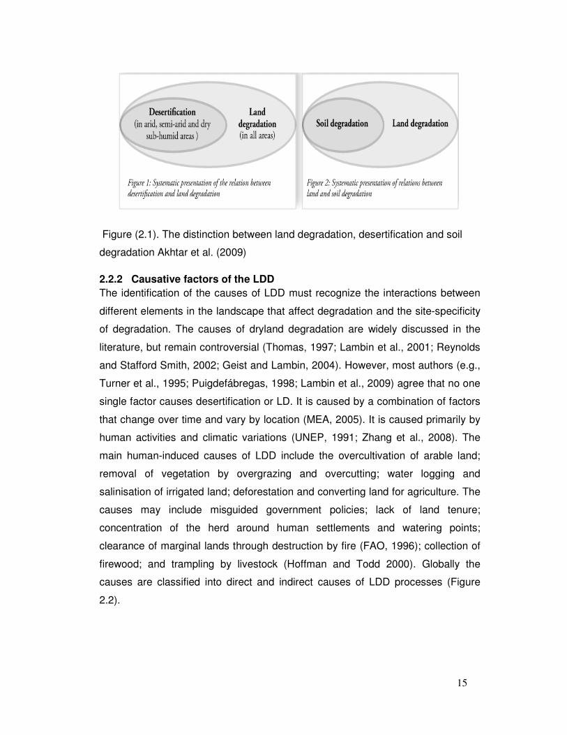
land and the expansion of the desert area (Balba, 1995). Akhtar et al. (2009), on
one hand, stated that LDD is often used synonymously with desertification
although LD occurs wherever land is not used sustainably – not only in arid and
semi-arid and dry sub-humid regions but also in humid and cold climates (see
Figure (2.1)). The interchangeable usage of “desertification” and “land
degradation” may be misleading since “land degradation” can be perceived as
“desertification”, that is, in drylands, or as a similar phenomenon or process in
non-drylands; on the other hand, stating LD and soil degradation are often used
synonymously, even though soil degradation is a more restricted term, focusing
on soil quality/fertility or soil productivity (see Figure (2.1)). The last context of
LDD termed by the report of Rio+20 is “land degradation and its subset
‘desertification’” (UNCCD, 2012). It is analogous, as Figure (2.1) shows.
15
Figure (2.1). The distinction between land degradation, desertification and soil
degradation Akhtar et al. (2009)
2.2.2 Causative factors of the LDD
The identification of the causes of LDD must recognize the interactions between
different elements in the landscape that affect degradation and the site-specificity
of degradation. The causes of dryland degradation are widely discussed in the
literature, but remain controversial (Thomas, 1997; Lambin et al., 2001; Reynolds
and Stafford Smith, 2002; Geist and Lambin, 2004). However, most authors (e.g.,
Turner et al., 1995; Puigdefábregas, 1998; Lambin et al., 2009) agree that no one
single factor causes desertification or LD. It is caused by a combination of factors
that change over time and vary by location (MEA, 2005). It is caused primarily by
human activities and climatic variations (UNEP, 1991; Zhang et al., 2008). The
main human-induced causes of LDD include the overcultivation of arable land;
removal of vegetation by overgrazing and overcutting; water logging and
salinisation of irrigated land; deforestation and converting land for agriculture. The
causes may include misguided government policies; lack of land tenure;
concentration of the herd around human settlements and watering points;
clearance of marginal lands through destruction by fire (FAO, 1996); collection of
firewood; and trampling by livestock (Hoffman and Todd 2000). Globally the
causes are classified into direct and indirect causes of LDD processes (Figure
2.2).

16
Figure (2.2). Global causes of LDD process (Lal et al., 1989).
2.2.2.1 Causative factors of vegetation and soil degradation
Deterioration in soil and plant cover has adversely affected nearly 50% of the land
area as a result of human mismanagement of cultivated and range lands (Dregne,
1986). Degradation processes begin generally with the degeneration of plant
communities. The degree of soil degradation determines vegetation cover, and it
is in many ways, a reflection of the state of vegetation. Vegetation patterns, which
share the landscape, affect the soil in all its dynamics, including water
redistribution over and within the soil, as well as their microbiological activity.
Biotic interactions generate and maintain soil structure in the top 20 cm of the soil
through the process of aggregation. This aggregation structure is a strong
determinant of the hydrological and biological soil characteristics (Thornes, 1995).
Thus, the erosive response of the soil is affected in terms of soil loss, runoff
generation, and nutrient loss after rainfall events.
The degradation of the vegetative cover of the soil may have both climatic and/or
anthropogenic origin (Poesen, 1995). Some human-induced causes leading to this
Global Causes of Land Degradation/Desertification
Indirect Causes
Human-induced Causes Human-induced Causes
. Climatic
conditions:
Rainfall
characteristics
Solar radiation
. Natural hazards
. Topography
features
. Vegetation cover
. Soil condition
. Overgrazing
. Inappropriate agricultural
Practices:
Over cultivation
Improper use of irrigation
water
Misuse of agrochemicals
. Deforestation
. Fire
. Industrial activities
. Urban expansion
. Land use patterns
. Poverty
. Increase of
population
. Tourism activities
. Government
policies
Direct Causes
Natural Causes
17
degradation process are forest removal by logging, bush fires, burning of crop
residues, overgrazing, and harvesting. The main natural causes affecting this
process, on the one hand, are the climatic conditions, explicitly aridity, which leads
to water stress causing a substantial reduction on the vegetation cover; and on
the other hand, the soil conditions and soil properties, such as soil depth or
organic matter content, both of which have a direct relationship on vegetation
cover (Kirkby and Kosmas, 1999).
The causative factors of soil degradation depend on the loss of actual or potential
productivity or utility as a result of natural or anthropogenic factors (Lal, 1997). It is
considered a global threat (Lal and Stewart, 1990), and it has strong impacts on
food and energy resources (Pimentel et al., 1976; Lal, 1988a) and environments,
as well as the greenhouse effect (Lal et al., 1995a, b; 1997a,b). Different forms of
degradation affect soils: physical, chemical, and biological degradation. Globally,
soil erosion, chemical deterioration, and physical degradation are the important
parts amongst various types of soil degradation. As a natural process, soil
degradation can be enhanced or dampened by a variety of human activities, such
as inappropriate agricultural management, overgrazing, and deforestation (Jie,
2002). Overgrazing is a serious factor in arid and semi-arid regions, causing soil
compaction and soil detachment in the sandy soil areas; consequently, it results in
wind erosion (Bilotta et al., 2007; Drewy et al., 2008).
2.2.3 Indicators of LDD (vegetation and soil)
Indicators can be referred to as quantitative or qualitative factors or variables that
provide a simple and reliable basis for assessing achievement, change or
performance, thus a unit of information measured over time that can help to show
changes in specific conditions. The use of indicators had a long history dating
back to early United Nations Initiatives in the 1970s (e.g., Enne and Zucca, 2000;
Grainger, 2009). The nature and role of desertification indicators can be
characterized as either individual or sets (Reynolds and Stafford Smith, 2002;
Renold et al., 2007). A given goal or objective can have multiple indicators (IFAD,
2002). Recently, numerous reports have documented various indicators for LDD
assessment. With regard to this study, the relevant indicators are as follows:
18
Biophysical indicators: these are described with respect to the soil properties (e.g.,
soil fertility, soil productivity, compaction, and loss of topsoil and subsoil); erosion
(e.g., shifting sands over fertile soils, water turbidity and sedimentation, soil loss,
and gullying incidence), land cover (e.g., land cover change and farming and
grazing intensity); and land form (e.g. topography) (Snel and Bot, 2002). Some
studies have shown that information related to many of the biophysical indicators
can be extracted from satellite imagery. Ustin et al. (2005) presents a review of
spectral characteristics of plants and soils that are detectable using optical
sensors and methods to identify and quantify properties that have the potential for
monitoring arid ecosystem processes. A range of spectral indices (calculated as
an arithmetic combination of the different spectral bands) that relates to vegetative
cover, biomass, soil properties, and so on are presented. This study relies on the
application of RS techniques for extracting some biophysical indicators, such as
vegetation and soil degradation status, to assess LDD in semi-arid areas.
Socioeconomic indicators: socioeconomic indicators refer to human factors
causing LDD, as well as the impact of LD on humans (Kuhlmann et al., 2002).
Due to the key role of poverty as a root cause, and the respective consequences,
which prove that LDD is more pronounced among the poorest segments of the
world population, socioeconomic indicators are framed by key characteristics of
poverty: lack of opportunity (e.g., lack of income, credit, land, and other assets of
attaining basic necessities such as food, clothing and shelter); insecurity (e.g.,
vulnerability to adverse shocks and limited means to cope); and disempowerment
(e.g., voicelessness and powerless to influence decisions) (Snel and Bot, 2002).
Institutional indicators: The main driving forces of LDD are institutional and policy
distortions, failures in the public or government, private or market, civil or
community sectors, and civil strife. Some of the indicators identified by Snel and
Bot (2002) include, for example, lack of institutional support, lack of participation,
transparency, and accountability, inadequate policies, and others.
2.2.4 Methods for LDD assessment
LDD assessment is a complex issue that involves many disciplines of natural and
social sciences. Stocking (1987) emphasized the difficulties associated with the
assessment of soil erosion, referring to the dynamic characteristics of LDD, the
19
problem of diverging frequencies and magnitudes, scales, limitations, and data
reliability. Earlier works on assessing LD are mainly carried out by focusing on the
assessment of the deterioration of the quality of soil. For instance, the GLASOD
and ASSOD projects have been orientated towards the assessment of soil
qualities. As the scientific concept of LDD evolved, many researchers realized that
the assessment of degradation should combine socioeconomic and institutional
indicators. The advancement of science and technology also created new
opportunities for such an assessment; for instance, RS and GIS technologies are
now applied widely to assess, monitor, and predict the type, extent, as well as
severity of land degradation (Ji, 2008). The principal methods for dry LDD
assessment (LADA, 2000) include expert opinion, remote sensing, assessment of
productivity change, field monitoring, sample studies at farmer level (based on
field criteria and expert opinion of land users), and modelling. In this study, RS
serves as a method for assessing LDD (more details in Chapter 3).
2.3 Arid and semi arid land in Sudan
Sudan has become the third largest country in Africa, covers an 1, 882,000 km2.
The dry lands (arid average annual rainfall less than 75 mm and semi-arid with
annual rainfall from 75mm to 300 mm), cover approximately 79% of the country
(1.5 million square kilometres), thus, constituting the largest area of dry lands in
Africa. The dry lands are faced with serious environmental and social- economic
problems such as drought, deforestation, poverty, famine and migration (Elfadl,
1997).
2.4 LDD in Sudan
2.4.1 Status and assessment of LDD
The region affected by drought and desertification in the Sudan is located
between the latitudes 12°N and 18°N and covers the country from the east to west
(DECARP, 1976).
The general awareness of desertification can be traced back to the early 1940s,
when a group of scientists and government officials (the Soil Conservation
Committee) raised a report calling for the need of fighting desert creep through
controlling the misuse of natural resources (NDDCU, 1999). Nevertheless, the
20
danger of environmental degradation was not publicly and officially appreciated.
Then Stebbing (1935) issued his book The Creeping Desert in Sudan and
Elsewhere in Africa, which highlighted the alarm progress of environmental
degradation in Sudan (NDDCU, 1999).
After the International Conference on Human and Environment in Stockholm
(1972), the Sudan declared its full support in combating desertification because
most of the country was already severely attacked by this phenomenon. Two-
thirds of the country’s area, about 650,000 square miles, was facing the problem
of being converted into deserts. In this particular area, the best grazing lands are
located and the largest part of traditional and modern agriculture is practiced.
There, 90% of Sudan’s cereals and oilseeds and 85% of its firewood requirements
are yielded (NDDCU, 1999).
In 1977, the Sudan submitted to the United Nations Conference on Desertification
(UNCOD) in Nairobi, Kenya, its program, which was drawn up in 1974 and
published in 1976. The program was called the Desert Encroachment Control and
Rehabilitation Program (DECARP). It divided the desert and semi-desert areas
affected by drought and desertification into five zones and formulated projects in
development for each zone and aimed to stop what was called desert
encroachment. Due to the difficulty in obtaining funds, only a few of the suggested
projects were started. The DECARP projects were modified to become
operational and oriented directly at combating desertification (NDDCU, 1999).
In the context of the assessment of LDD in the Sudan, after the first report of
1944, the Department of Land Use and Rural Development undertook sporadic
studies of LU and resource degradation in the 1950s and 1960s. In 1975, the
National Council for Research and the Ministry of Agriculture with financial
assistance from the UN and IUCN conducted an air born and car-based field
survey to assess the most recent changes in the desert encroachment in northern
Sudan (Lamprey, 1975). In his well-known study, Lamprey (1975) reported that
the southern margin of the Sahara in western Sudan was advancing at a rate of
approximately 5.5 km per year. However, this study was not supported by enough
scientific evidence (Middleton, 1997). Lamprey’s conclusions were scrutinized by
a team from the University of Lund, Sweden in co-operation with the University of
21
Khartoum by conducting a series of investigations under a project called Regional
Studies of Desertification and its Control during the period 1981–85. The general
goal was to develop, test, and apply monitoring methods for the understanding
and prediction of desertification (Hellden, 1988). Detailed studies combining the
analysis of aerial photography and satellite imagery data, published records, and
field studies showed no progressive spread of desertification (Olsson 1983;
Hellden, 1988).
Scientists from the United States (U.S.) used satellite data of the 1980s and
1990s to compare NDVI data of the drought period of 1984 with the wet season of
1985, and reported that biomass fluctuated in response to annual rainfall and that
the fringes of the Sahara desert were oscillating from north and south depending
on the annual rainfall, the Kordofan and Darfur regions included. Though the 1984
drought had triggered a recent process of desertification in the Sudan, gaps exist
in knowledge on the process of desertification. Sudanese scientists undertook
small scale and sectoral work on desertification assessment in the late 1980s and
early 1990s in response to the drought incidents of the 1980s, and 1990s and in
response to the requests of the Agenda 21 and the UN Convention to Combat
Desertification. The work was compiled by English et al. (1997) and provides a
systematic base study that can serve as a starting point for continued (periodical)
monitoring and assessment of desertification in the Sudan.
Several case studies have been carried out to support the assessment of LDD in
several regions and worldwide, including the Sudan (UNEP 1977; FAO/UNEP
1984; UNEP/ISRIC (GLASOD) 1990; Dregne 1991; Glover 2005). According to
Ayoub (1998), it can be concluded that excluding the hyperarid zone of the
agricultural land, pasture and forest and woodland (170 million ha in total), human
factors have degraded nearly 75 million ha (45%). The highest estimate was that
of Dregne (1991), while the estimates of UNEP (1977) and the FAO/UNEP (1984)
were similar. The GLASOD soil assessment shows that severe and very severe
degradation in Sudan totalled 58 million ha. This may indicate that desertification
in the Sudan is more linked to soil degradation than to vegetation degradation.
The GLASOD methodology of assessment of human-induced soil degradation
22
was considered a definite progress compared with those used in other
assessments (Thomas and Middleton 1994).
According to Ayoub (1998), about 64 million ha of soils is degraded in the Sudan.
Eighty-one percent of the total degraded area is in susceptible dry lands (arid,
semi-arid, and dry sub-humid). Most of the degradation (74% of the total degraded
soils) is in the arid and semi-arid zones, but significant land areas are also
degraded in the dry sub-humid and moist sub-humid zones. Represented as
percentage of total area per aridity zone, the dry sub-humid and moist sub-humid
zones have figures higher than the semi-arid and hyper-arid zones, with 28% and
29%, respectively.
2.4.2 Causative factors of LDD in Sudan
In Sudan, the most destructive effects of human activities leading to natural
resources degradation and causing desertification result from droughts, coupled
mainly with extended rain-fed agriculture on marginal lands, with overgrazing,
wood cutting, deforestation, uprooting of shrubs, and the burning of grasslands
and forest shrubs. It may ultimately be concluded that a combination of factors
affecting fragile ecosystems, which exist under harsh climatic conditions,
especially human activities that are increasing with irreversible magnitude, are the
actual causes of desertification in the Sudan (DECARP, 1976).
The causes of LDD, among others, can be traced back to the still growing need
for firewood (Ayoub 1998). It is reported that the Sudan derives more than 75% of
its energy requirements from fuelwood, estimated at 22 million m3 per year (WRI,
1994). Ayoub (1998) stated that this is equivalent to about 400 million acacia trees
being cut annually.
Another cause of LDD in the Sudan is the clearance of rangelands for rain-fed
agriculture and for shifting cultivation. According to the FAO (2001b), during the
1980s and 1990s, there was a rapid expansion of rain-fed mechanized cultivation
with the aim of attaining self-sufficiency in production. According to Salih (1987),
the land area for mechanized agriculture increased from about 2.0 million ha in
1954 to about 14 million ha in 1994, a rate of 300,000 ha per year. Large-scale
farming has been the main factor contributing to deforestation and consequently
to LD (FAO 2001a; Glover 2005).
23
Rangeland fires, deliberately set by herders to improve grazing, consume annually
about 35% of the natural range land product, estimated to be equivalent to 300
million tons of biomass (fodder) (Elmoula, 1985). Ayoub (1998) concluded that
overgrazing (47%), improper agricultural practices (22%), deforestation for
firewood and for urban demand of charcoal (19%), and overexploitation of
vegetation for domestic use (13%) were the major causes of LDD in the Sudan
(Kordofan and Darfur). About 88,000 ha of woodlands was cleared each year for
conversion to agriculture.
The war in Sudan has caused a large population displacement and increased
population pressure on available resources leading to LDD (Kibreab, 1996). Also,
there has been an influx of migrants from neighbouring countries (Chad, Eritrea)
into Sudan due to war and drought, affecting the land resources, particularly
around respective camps.
2.4.3 Status and causative factors of vegetation and soil degradation
The vegetation in Sudan covers a broad range of phyto-geographical and
ecological zones; those are closely associated with specific plant species that
favour specific climatic zones with basic vegetation still existing in most areas (D-
JAM, 2006). However, misuse and overuse of natural resources in different
regions of the country have resulted in LU and vegetation cover changes that
have reduced the density of plant species in the regions (D-JAM, 2006). Changes
have been caused by increased deforestation, agricultural crop cultivation,
overgrazing, and migration of people due to the increasing impact of war and
violence and drought in some of the regions, with current estimates that about half
of the country is exposed to periodic waves of drought (Abbadi and Ahmed, 2006;
Symeonakis et al., 2004).
Human induced reduction in vegetation cover, poor agricultural practices, and
drought has led to soil aggregate breakdown and soil matter losses, while poor
irrigation practices have lead to salinization, thus to an increase of the rate of soil
erosion and to the increasing incidence of desertification (Symeonakis et al.,
2004). Overgrazing through livestock pasture has a negative impact on the soil
structure through trampling and compaction of the soil, thus reducing infiltration
and increasing the rate of runoff, while the effect of deforestation also reflects
24
through increasing surface runoff, as it removes the vegetation cover
(Symeonakis et al., 2004). The percentage of the total land area that has
experienced a level of degradation is estimated at 23% in 1988; 7.2% recorded as
lightly degraded, 14.4% as moderately degraded, and 1.4% as strongly degraded
(UNDESA, 2007).
2.4.4 Biophysical and socioeconomic indicators of LDD in Sudan
The biophysical and socioeconomic indicators of LDD in the Sudan can be
monitored by the destruction of soil productivity, erosion of topsoil, gullying, dust
storms, moving sand dunes, declining crop yields, loss of biodiversity, diminishing
of surface water resources, localised areas of food insecurity, poverty,
malnutrition, conflicts, and mass migration. The devastating droughts of 1984 and
1990, which showed long periods of low rainfall conditions, aggravated the
situation (Karrar, 2002).
2.5 Effects of the LUC on LDD
2.5.1 In general
“Land use” (LU) is the human use of land. LU involves the management and
modification of natural environment or wilderness into building environments, such
as fields, pastures, and settlements. LU has also been defined as the
arrangements, activities, and inputs people undertake in a certain land cover type
to produce, change, or maintain it (FAO, 1997; FAO/UNEP, 1999). LU denotes
how humans use the biophysical or ecological properties of land. LU includes the
modification and/or management of land for agriculture, settlements, forestry, and
other uses, including those that exclude humans from land, as in designation of
nature reserves for conservation (Erle, 2010).
The term “land cover” and “land use” are often confused. Land cover is ‘the
observed physical and biological cover of the earth’s land, as vegetation or man-
made features.’ In contrast, ‘land use is the total of arrangements, activities, and
inputs that people undertake in a certain land cover type’ (FAO, 1997;
FAO/UNEP, 1999). LU change is the use of a particular land and its change over
time, (e.g., from natural vegetation/forest to cultivation; cultivation to grazing or
from swamp to cultivation) (Joseph, 2004). Most causative factors of LDD
25
mentioned above, such as deforestation, overcutting, overgrazing, and burning
fire, represent human activities for utilizing land recourses affecting LD
horizontally and vertically. It is estimated that about 6 million km2 of
forest/woodlands and 4.7 million km2 of savannas/grasslands/steppes were
cleared during the period from 1850 to 1992 (Ramankutty and Foley, 1999). From
2000 to 2010, the forest area decreased by 13 Mha . Yr-1 (FRA, 2010). Cropland
increased from 265 Mha in 1700 to 1471 Mha in 1990 (Goldewijk, 2001).
Synergistic causing factors of LUC or/and LDD
The current LU of any region is mainly a result of long-term historical, social,
economical, cultural, political, climatic, environmental, and even religious factors,
all of which are implicated in the changes of ownership and tenure, population
growth, and urban-industrial development.
LU change is always caused by multiple interacting factors originating from
different levels of organization of the coupled human-environment systems. The
mix of driving forces of LU changes varies in time and space, according to specific
human-environment conditions. Driving forces can be slow variables, with long
turnover times, which determine the boundaries of sustainability and collectively
govern the LU trajectory (such as the spread of salinity in irrigation schemes or
declining infant mortality), or fast variables, with shorter turnover times (such as
food aid or climatic variability associated with El Nino oscillation). Biophysical
drivers may be as important as human drivers. Changes are generally driven by a
combination of factors that work gradually and factors that happen intermittently
(Lambin, 2001). Liang (2012) stated that the drivers of LC/LU changes include
local and proximate physical, socioeconomic, and demographic factors, as well as
broader global and regional climatic or macroeconomic forces of change.
2.5.2 Effects of LUC on LDD in Sudan
The FAO performed the recent land cover atlas and percentage of the Sudanese
land cover after separation of Southern Sudan showing that the area of bare rocks
and soil is 50.7%, herbaceous is 13.8%, agricultural area is 12.6%, shrub area is
11.8%, and trees is 10% (FAO, 2012) (see Figure (2.3)).
26
Urban and rural land use: An estimated 40.8% of the country’s population lives in
the urban areas that have witnessed an increasing trend in their growth rate over
the years: 59.2% of the population live in the rural areas (UNDESA, 2007).
The growth in the urban population may be related to the large movement of
displaced groups, who have moved into the peripheral areas of the major cities in
the country, which are characterized by over population with limited access to
water and basic amenities (Musa et al., 1999). The incidence of drought and
famine has also encouraged the migration of people to the urban centres in
search of paid employments and opportunities fora better standard of living.
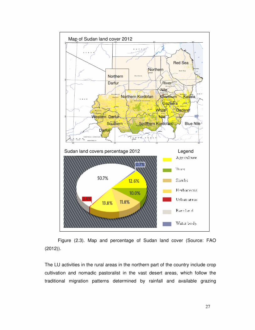
27
Map of Sudan land cover 2012
Red Sea
Northern
Northern
Darfur River
Nile
Northern Kordofan Khartoum Kasala
Gazeera
White Gadaref
Western Darfur Nile
Southern Southern Kordofan Blue Nile
Darfur
Sudan land covers percentage 2012 Legend
Figure (2.3). Map and percentage of Sudan land cover (Source: FAO
(2012)).
The LU activities in the rural areas in the northern part of the country include crop
cultivation and nomadic pastoralist in the vast desert areas, which follow the
traditional migration patterns determined by rainfall and available grazing
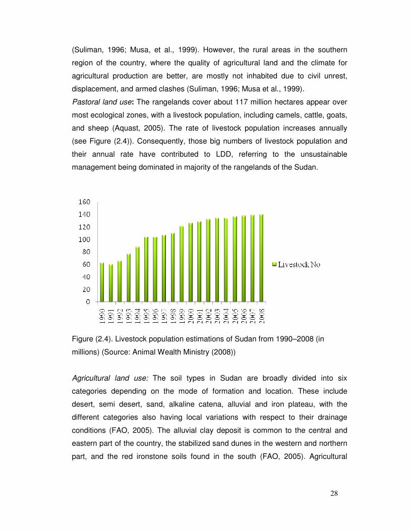
28
(Suliman, 1996; Musa, et al., 1999). However, the rural areas in the southern
region of the country, where the quality of agricultural land and the climate for
agricultural production are better, are mostly not inhabited due to civil unrest,
displacement, and armed clashes (Suliman, 1996; Musa et al., 1999).
Pastoral land use: The rangelands cover about 117 million hectares appear over
most ecological zones, with a livestock population, including camels, cattle, goats,
and sheep (Aquast, 2005). The rate of livestock population increases annually
(see Figure (2.4)). Consequently, those big numbers of livestock population and
their annual rate have contributed to LDD, referring to the unsustainable
management being dominated in majority of the rangelands of the Sudan.
Figure (2.4). Livestock population estimations of Sudan from 1990–2008 (in
millions) (Source: Animal Wealth Ministry (2008))
Agricultural land use: The soil types in Sudan are broadly divided into six
categories depending on the mode of formation and location. These include
desert, semi desert, sand, alkaline catena, alluvial and iron plateau, with the
different categories also having local variations with respect to their drainage
conditions (FAO, 2005). The alluvial clay deposit is common to the central and
eastern part of the country, the stabilized sand dunes in the western and northern
part, and the red ironstone soils found in the south (FAO, 2005). Agricultural
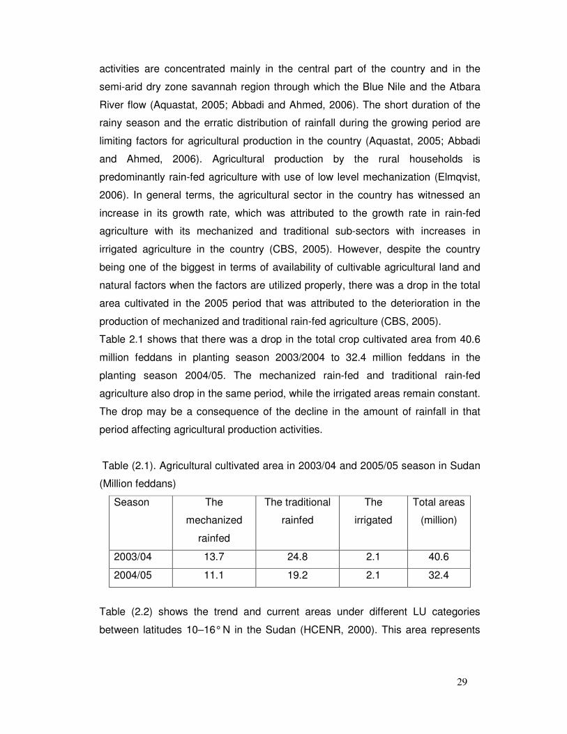
29
activities are concentrated mainly in the central part of the country and in the
semi-arid dry zone savannah region through which the Blue Nile and the Atbara
River flow (Aquastat, 2005; Abbadi and Ahmed, 2006). The short duration of the
rainy season and the erratic distribution of rainfall during the growing period are
limiting factors for agricultural production in the country (Aquastat, 2005; Abbadi
and Ahmed, 2006). Agricultural production by the rural households is
predominantly rain-fed agriculture with use of low level mechanization (Elmqvist,
2006). In general terms, the agricultural sector in the country has witnessed an
increase in its growth rate, which was attributed to the growth rate in rain-fed
agriculture with its mechanized and traditional sub-sectors with increases in
irrigated agriculture in the country (CBS, 2005). However, despite the country
being one of the biggest in terms of availability of cultivable agricultural land and
natural factors when the factors are utilized properly, there was a drop in the total
area cultivated in the 2005 period that was attributed to the deterioration in the
production of mechanized and traditional rain-fed agriculture (CBS, 2005).
Table 2.1 shows that there was a drop in the total crop cultivated area from 40.6
million feddans in planting season 2003/2004 to 32.4 million feddans in the
planting season 2004/05. The mechanized rain-fed and traditional rain-fed
agriculture also drop in the same period, while the irrigated areas remain constant.
The drop may be a consequence of the decline in the amount of rainfall in that
period affecting agricultural production activities.
Table (2.1). Agricultural cultivated area in 2003/04 and 2005/05 season in Sudan
(Million feddans)
Season The
mechanized
rainfed
The traditional
rainfed
The
irrigated
Total areas
(million)
2003/04 13.7 24.8 2.1 40.6
2004/05 11.1 19.2 2.1 32.4
Table (2.2) shows the trend and current areas under different LU categories
between latitudes 10–16° N in the Sudan (HCENR, 2000). This area represents
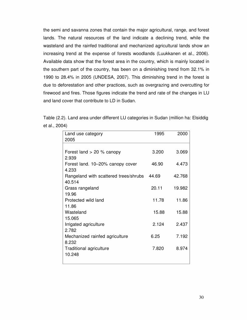
30
the semi and savanna zones that contain the major agricultural, range, and forest
lands. The natural resources of the land indicate a declining trend, while the
wasteland and the rainfed traditional and mechanized agricultural lands show an
increasing trend at the expense of forests woodlands (Luukkanen et al., 2006).
Available data show that the forest area in the country, which is mainly located in
the southern part of the country, has been on a diminishing trend from 32.1% in
1990 to 28.4% in 2005 (UNDESA, 2007). This diminishing trend in the forest is
due to deforestation and other practices, such as overgrazing and overcutting for
firewood and fires. Those figures indicate the trend and rate of the changes in LU
and land cover that contribute to LD in Sudan.
Table (2.2). Land area under different LU categories in Sudan (million ha: Elsiddig
et al., 2004)
Land use category 1995 2000 2005 Forest land > 20 % canopy 3.200 3.069 2.939 Forest land. 10–20% canopy cover 46.90 4.473 4.233 Rangeland with scattered trees/shrubs 44.69 42.768 40.514 Grass rangeland 20.11 19.982 19.96 Protected wild land 11.78 11.86 11.86 Wasteland 15.88 15.88 15.065 Irrigated agriculture 2.124 2.437 2.782 Mechanized rainfed agriculture 6.25 7.192 8.232 Traditional agriculture 7.820 8.974 10.248
31
Synergistic-causing factors of LUC or/and LDD
Poverty: affects how land users manage their land. It reduces the options
available, ruling out some conservative practices because they require too much
investment of land, labour, and capital (Stock and Murnaghan, 2001). Poor people
generally have no choice but to opt for immediate benefit, very often at the
expense of long-term sustainability (Barrow, 1994). Therefore, if a community is
too poor to raise the capital needed for restoration of degraded land, then
degradation is likely to continue and accelerate (Warren and Agnew, 1988). Thus,
poverty induces LDD, which, in turn, reinforces poverty leading to further LDD and
so on (UN Center on Transnational Corporation, 1985). Nowadays, the World
Bank recognised this problem as a necessary policy in the Third World (Hopper,
1988).
In the Sudan, poverty represents a high percentage among the people; however,
there is no accurate information to confirm that. The majority of poor centralize in
rural areas. Poor communities in rural dry areas depend on their fragile eco-
system for sustenance. They rely on natural vegetation for making homes, animal
enclosures, and for the provision of energy. Because of poverty, they are deprived
of the use of modern technical tools and are pushed into the vicious circle of
poverty. These factors can contribute to increasing LDD (Mustafa, 2007).
Increase of population: Population has been one of the most frequently cited
causes of LDD (Barrow, 1994). What is more important in terms of LDD is the rate
of change of population and settlement patterns, instead of the exponential
increase (Pérez-Trejo, 1994). In the Sudan, there are always increasing in
population growth: its rate is approximately 2.5% annually, and moreover, there is
no stability among some population due to the war and to other socioeconomic
problems. This leads to displacement and seeking the stable life near the cities
and areas rich in natural resources. These factors contribute to LUC and/or LDD.
In addition, in Sudan, the livestock population is increasing, therefore, it is
considered one of the driven factors of LUC and LDD, due to the domination of
unsustainable management of the rangeland.
Government policies: There are specific policies at local, regional, and more
global scale, related to land protection, such as policies supporting terracing,
32
policies favouring extensive agriculture, coastal protection policies, and so on, but
their effectiveness depends on the degree to which they are enforced. In the
Sudan, policies and laws related to land protection exist; however, most of them
are not enforced. This situation encourages land resource deterioration by misuse
of the land, particularly in marginal area in semi-arid regions.
Land tenure: Bruce (1993) defined tenure as a set of rights which a person or
some private or public entity holds in land or trees as recognized by law or custom
in particular societies. Tenure rights are usually defined by statements of
ownership, usufruct, lease, or contracts.
In most of the rural areas of western Sudan, tenure rights for land, trees, and
pasture come from customary laws or indigenous traditions usually based on tribal
structure. Different groups, whether sedentary or pastoralists, have developed
tenure and usufruct rights to trees and other critical resources, such as water and
grassland available for dry-season grazing, within their territories under the tribal
management system. They minimize opportunities for over-use and degradation
(Luukkanen. et al, 2006). However, negative behaviours and manners may
contribute to environmental degradation, such as governance of the owners of the
lands by one system of LU that can deteriorate the land and local environment, for
example, abandonment of land after overuse and neglect of fallow, leaving the
land bare and exposed to wind or water erosion.
33
Chapter Three
RS and GIS Applications in Land Use and Land Degradation/Desertification
3.1 Background
3.1.1 Remote sensing
Remote sensing (RS) is the science and art of obtaining information about an
object, area, or phenomenon through the analysis of data acquired by a device
not in contact with the object, area, or phenomenon under investigation (Lillesand
et al., 2008). The expression “remote sensing” was coined by geographers at the
U.S. Office of Naval research in the 1960s at about the time that the use of spy
satellites was beginning to move out of the military sphere and into the civilian
sphere (Cracknell and Hayes, 2007). In a broader context, RS activities
encompass a multitude of activities, and subsequent data processing,
interpretation, and dissemination of the processed data and image products
(Chuvieco and Heute, 2010). RS is usually used in a more restricted sense in
which the observation is made from above the object of interest by a sensor
carried on an airborne or spaceborne platform, and the information is carried by
electromagnetic radiation, that is, visible light, infrared or ultraviolet radiation, or
radio waves (Rees, 2006). This radiation can occur naturally, in which case, the
type of RS is said to be passive, or it can be transmitted from the sensor to the
object under investigation, in which case the RS is said to be active. Passive RS
developed originally from aerial photography and later included other parts of the
electromagnetic spectrum, other technologies for detecting the radiation and
storing the data, and other platforms to carry the sensor. Active RS grew from the
military development radar during the Second World War (Rees, 2010).
RS as a technology and methodology has evolved historically in parallel with other
technological advancements, such as the improvement in sensor electronics,
satellite platforms, transmission systems, and computer data processing. These
developments have resulted in progress in the quantity, quality, and diversity of
data available to the scientific community (Chuvieco and Huete, 2010). RS
applications cover a range of topics, including archaeology, agriculture,
cartography, civil engineering, meteorology, climatology, coastal studies,
34
emergency response, forestry, geology, GISs, natural and man-made hazards,
LU, land cover, natural disasters, oceanography, and water resources (Gamba
and Herold, 2010). The ‘work horses’ of satellite data generation, such as the
Landsat and System Pour 1´Óbservation de la Terre (SPOT) satellites or the
Advanced Spaceborne Thermal Emission and Reflection Radiometer (ASTER)
and Moderate Resolution Imaging spectrometer (MODIS) instruments, have
become important in global and regional studies of biodiversity, nature
conservation, food security, deforestation impact, desertification monitoring, and
other application fields.
With the increasing spatial resolution of the ‘1-m generation’ of IKONOS
(launched in 1999), QuickBird (2001), or OrbView (2003) sensors, new application
fields, previously the domain of airborne RS, could be tackled by satellite RS
(Blaschke, 2009). In 2007, the first commercial satellite with a resolution of less
than half a meter (Worldview-1; 0.44 m panchromatic) became operational,
followed by multispectral sensors, such as GeoEye-1 (2008) and Worldview-2
(2009), providing pan-sharpened sub half-meter resolution image data. At present,
vehicle detection, urban mapping, and vegetation assessment applications are
developing rapidly in terms of both numbers and effectiveness (Blaschke et al.,
2011). On the other hand, the generation of new versions of software is ongoing
(ERDAS Imagine 9.3, ENVI and Defniens or eCognition) for digital image analysis.
Recently, Object-Based Image Analysis (OBIA) or Geospatial Object-Based
Image Analysis (GEOBIA) have become a more improved analysis approach than
traditional pixel-based image analysis.
3.1.2 Integration of RS and GIS
RS is a technology whose development has been heavily conditioned by the U.S.
federal government. On the contrary, GIS development has been influenced
primarily by commercial enterprises. In both RS and GIS, digital processing began
to become important in the 1960s and 1970s. Indeed, even the terms describing
these two technologies were created virtually about the same time. Evelyn Pruitt
of the U.S. Office of Naval Research coined the term “remote sensing” in 1958.
Roger Tomlinson is credited with the term “geographic information systems” in
1962, when he was working for a Canadian photogrammetric engineering firm
35
(Star et al., 2010). GIS can be defined as a set of programs that store, manage,
manipulate, and represent data with some kind of spatial component (Burrough
and McDonell 1998; Longely et al., 2005). The integration of spatial information
has been remarkably favoured by the spectacular development of the technology
of GIS (Chuvieco and Huete, 2010). The integration of RS and GIS in
environmental applications has become increasingly common in recent years. RS
imagery is an important data source for environmental GIS applications and
conversely, GIS capabilities are being used to improve image analysis procedures
(Hinton, 1996). Increased collaboration between RS and GIS researchers has led
to an increased cross-fertilization of research ideas and information of new
research agendas for both the GIS and RS communities (e.g., Star, 1991;
ASPRS, 1994; Legg, 1994; Sample et al., 1997).
Chuvieco and Huete (2010) stated that the increasing convergence between RS
and GIS is justified, among others, for the following reasons:
• Both have a clear territorial interest.
• They have similar hardware and software requirements.
• Many professionals commonly use both technologies.
• They have similar research demands, as in the case of error analysis, the
structure of and access to the data, the development of computer
hardware, and the interpretive methodology (Star et al., 1991).
3.2 Applications of RS and GIS in land use change and land degradation in
dryland
Multispectral RS has been used to identify changes in LU in desert areas. For
instance, areas of active agriculture stand out in high contrast to the low-cover
desert around them. This can make agricultural LU particularly easy to identify in
arid regions. Following this approach, Ray (1995) used LandSat Thematic Mapper
and Multispectral Scanner (MSS) images from 1973 to 1991 to document the
history of agriculture in a portion of the Mojave Desert of California (see also Okin
et al., 2001a). Ram and Kolarkar (1993) used MSS, TM, and data from the Indian
Remote Sensing1 (IRS-1) satellite, along with earlier maps of LU to evaluate LUC
in parts of the arid regions in India.
36
In studies of protected versus degraded areas, Otterman (1996) and Tsoar and
Karnieli (1996) found that vegetation is the cause of reduced reflectance in
degraded areas with bright sandy soils. Karnieli and Tsoar (1995) and Tsoar and
Karnieli (1996) have also suggested that the tendency of disturbed sandy desert
areas to be brighter than undisturbed areas is due to the loss of cover of the soil
by cryptobiotic crust.
The low cover of vegetation often found in semi-arid areas has prompted many
authors to concentrate on the soil surface – as opposed to the vegetation cover –
to indicate the state of the land surface. For example, Paisely et al. (1991) showed
that active dunes are brighter than inactive stabilized dunes in all spectral bands;
their results indicated that in dune areas susceptible to wind erosion, vegetation
cover is often too low to make an appreciable contribution to the apparent surface
reflectance. Okin et al. (2001a) showed that areas of wind erosion stand out
clearly as bright streaks against darker stable soils. These sand blowouts are
indicative of degradation of the environment and a suite of biotic and abiotic
processes that result from disturbance of the stable soil surface.
Hill and Schutt (2000) found that soil surface reflectance was inversely related to
the concentration of organic carbon in surface soils. Soils rich in organic carbon
tended to be of higher quality or less degraded than carbon-poor soils.
Parameterizing soil reflectance spectra with variables related to specific shape
characteristics of the spectral profile permits organic carbon concentrations in
soils to be estimated on the basis of regionally. Recently, Biro (2012) addressed
the potential of applying multi-sensor RS data for mapping LU/LC and their trends
of change in the African Sahel in the Sudan. Also, the impacts of the present
LU/LC types on soil properties were assessed through soil sampling and
measurements in the African Sahel in the Sudan.
3.3 RS and GIS for mapping and obtaining information of LU and LDD
Data are a collection of observations, or raw, unprocessed values or sets of
values. Information is data within a given context. Without the context, the data
are usually meaningless (Borengasser et al., 2008). Remotely sensed data can be
characterized by the image spatial resolution (pixel size), spectral resolution
(wavelength utilized), temporal resolution (when and how often imagery is
37
collected), and radiometric resolution (the degree of differentiation within the
dynamic range of the sensor) (Warner et al., 2010). RS is applied for many
purposes: mapping, study of responses and consequences, and impact
assessment of the LC/LUC (Liang, 2012).
3.3.1 Image classification
Image classification is an important process for quantifying the location, extent,
and trends of LC/LUC. Since the mid-1960s, humans have been able to extract
LU/LC and biophysical information directly from RS data using digital computers
and special-purpose image classification algorithms (Jensen et al., 2009). The
objective of these operations was to replace visual analysis of the image data by
quantitative techniques of automatisation of the identification of features in the
image. The analysis of multispectral image data involves the application of
statistical-based decision rules for determining the LC of each pixel in an image
(Lillesand et al., 2008). Many potential variables may be used in image
classification, including spectral signatures, vegetation indices, transformed
images, textural or contextual information, multitemporal images, multisensory
images, and ancillary data (Price, Guo, and Stiles, 2002). Selection of a suitable
classification algorithm is one of the important steps for performing desirable class
results. In general, image classification approaches can be grouped into different
categories: supervised versus unsupervised; parametric versus nonparametric;
hard versus soft (fuzzy) classification; per-pixel, sub-pixel, and per-field (Lu and
Weng, 2007). This study addresses per-pixel classification (hybrid classification)
versus per-field or object classification (fuzzy logic classifier) for quantifying and
mapping the LU/LC changes (LDD). Biophysical indexes are used for determining
and assessing LDD.
3.3.1.1 Vegetation and soil indices for LDD assessment
Vegetation indices (VIs) are simple and robust techniques for extracting
quantitative information on the amount of vegetation, or greenness, for each pixel
in an image. VIs typically involve spectral transformation of two or more bands:
one in the chlorophyll-absorbing red spectral region (0.6–0.7 µm) and the other in
the non-absorbing NIR (0.7–1.1 µm). The two bands are combined in a manner
that enhances the vegetation signal, while minimizing non-vegetation influences
38
(Chuvieco and Huete, 2010). In contrast to PCA and other techniques, VIs are
designed to provide information on only one feature in an image: vegetation
greenness. As a result of simplicity, VIs have proved to be among the most robust
techniques in RS, yielding consistent spatial and temporal comparisons of green
vegetation at local to global scale (Chuvieco and Huete, 2010).
The most commonly used index, the normalized difference vegetation index
(NDVI), successfully indicates vulnerable areas and assesses changes in a
qualitative way (Justice et al., 1985; Bolle, 1994). However, inter-annual changes
of vegetation cover in dry regions expressed by NDVI values can reflect rainfall
fluctuation (Tucker et al., 1991; Nicholson et al., 1998; Williams, 2000). The soil
background affects NDVI, especially in semi-arid and arid environments, where
there is less than 30% plant cover (Pech et al., 1986; Major et al., 1990). For
reducing the soil background effect, many vegetation indices, such as the
weighted difference vegetation index (WDVI) by Clevers (1989), soil-adjusted
vegetation index (SAVI) by Huete (1988), and MSAVI, the modified version of
SAVI (Qi et al., 1994), were introduced. Both SAVI and MSAVI use soil
adjustment factors, thus they are not functionally equivalent to NDVI and contain
different information on vegetation characteristics (Baret et al., 1989). The
atmospherically resistant vegetation index (ARVI) was developed to remove the
influence of aerosols through the use of the blue band (B) (which is the most
sensitive to atmospheric haze) to correct for aerosol effects on the red band as
well as the soil-adjusted atmospheric resistant vegetation index (SARVI)
(Kaufman and Tanre, 1992). The ARVI adjusts to atmospheric interference and
the SARVI corrects for both atmosphere and soil interference.
Lu et al. (2004) and (2011) found that VIs with TM SWIR band 5 had higher
correlation coefficients than those without band 5, such as a normalized difference
vegetation index (NDVI), when they examined the relationship between VIs and
forest stand structure attributes, such as biomass, volume, and average stand
diameter, in different biophysical conditions in the Brazilian Amazon. Examples of
VIs with band 5, such as ND4-25, ND42-53, and ND42-57, are highlighted in
Table (3.3)
39
In the soil, many different indices have been found and developed by scientists,
such as a red index (RI) detecting soil surface colour changes, due to the
presence of more reddish soil materials, and Hematite content (Escadefal et al.,
1989; Ray et al., 2005). Bare soil index (BSI) is commonly used to evaluate
desertification processes. It increases as bare soil exposure increases (Rikimary
and Miyatake, 1997). Xiao et al. (2006) proposed a new index, topsoil grain size
index (GSI), which is associated with the mechanical composition of topsoil. GSI
indicates the coarsening of a topsoil grain size, which has a positive correlation
with fine sand content. This class of sand is dominated by the finer sizes of sand
particle, and somewhat less coarse than either sand or the coarse sand of a
surface soil texture, as a manifestation of undergoing desertification. The more
severe the desertification, the coarser the topsoil grain size composition; grain
size refers to the mean or the effective diameter of individual mineral grains or
particles. Overgrazing is one of the causes of soil coarsening due to accelerating
soil erosion by wind (Fu et al., 2002). Table (3.3) shows the formulae of the above
mentioned indices.
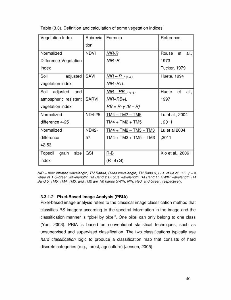
40
Table (3.3). Definition and calculation of some vegetation indices
NIR – near infrared wavelength; TM Band4, R-red wavelength; TM Band 3, L- a value of 0.5 γ – a value of 1 G-green wavelength; TM Band 2 B- blue wavelength TM Band 1; SWIR wavelength TM Band 5. TM5, TM4, TM3, and TM2 are TM bands SWIR, NIR, Red, and Green, respectively.
3.3.1.2 Pixel-Based Image Analysis (PBIA)
Pixel-based image analysis refers to the classical image classification method that
classifies RS imagery according to the spectral information in the image and the
classification manner is “pixel by pixel”. One pixel can only belong to one class
(Yan, 2003). PBIA is based on conventional statistical techniques, such as
unsupervised and supervised classification. The two classifications typically use
hard classification logic to produce a classification map that consists of hard
discrete categories (e.g., forest, agriculture) (Jensen, 2005).
Vegetation Index Abbrevia
tion
Formula Reference
Normalized
Difference Vegetation
Index
NDVI NIR-R
NIR+R
Rouse et al.,
1973
Tucker, 1979
Soil adjusted
vegetation index
SAVI NIR – R * (1+L)
NIR+R+L
Huete, 1994
Soil adjusted and
atmospheric resistant
vegetation index
SARVI
NIR – RB * (1+L)
NIR+RB+L
RB = R- γ (B – R)
Huete et al.,
1997
Normalized
difference 4-25
ND4-25
TM4 – TM2 – TM5
TM4 + TM2 + TM5
Lu et al., 2004
, 2011
Normalized
difference
42-53
ND42-
57
TM4 + TM2 – TM5 – TM3
TM4 + TM2 + TM5 + TM3
Lu et al 2004
,2011
Topsoil grain size
index
GSI R-B
(R+B+G)
Xio et al., 2006
41
Unsupervised classification
Unsupervised classification: the identities of land cover types to be specified as
classes within a scene are not generally known a priori because ground reference
information is lacking or surface features within the scene are not well defined.
The computer is required to group pixels with similar spectral characteristics into
unique clusters according to some statistically determined criteria (Duda et al.,
2001). The analyst then relabels and combines the spectral clusters into
information classes.
The unsupervised training is based on selecting the discrimination space (set of
bands that will be used for the grouping) and the clustering algorithm.
Supervised classification
Supervised classification is the technique most often used for the quantitative
analysis of RS image data. At its core is the concept of segmenting the spectral
domain into regions that can be associated with ground cover classes of interest
to a particular application. In practice, those regions may sometimes overlap
(Richards, 2013).
In supervised classification, the identity and location of some of the land cover
types (e.g., urban, agriculture, or wetland) are known a priori through a
combination of field work, interpretation of aerial photography, map analysis, and
personal experience (Hodgson et al., 2003). The analyst attempts to locate
specific sites in the remotely sensed data that represent homogeneous examples
of these known land cover types. These areas are commonly referred to as
training sites because the spectral characteristics of these known areas are used
to train the classification algorithm for eventual land cover mapping of the
remainder of the image (Jensen, 2005). Most researchers prefer supervised
classification because it generally gives more accurate class definitions and
higher accuracy than unsupervised approaches (Fundamental of Remote
Sensing, 1999). Three statistical classifiers are in general use: the parallelepiped
method, minimum distance classifier, and the maximum likelihood algorithm
(Mather and Brand, 2009).
Maximum Likelihood Classifier (MLC)
42
Maximum likelihood classification (MLC) is one of the most common supervised
classification techniques used with remote image data and was the first rigorous
algorithm to be employed widely. Even after 40 years of use, MLC is still the
workhorse of supervised image classification (Warner et al., 2010), and it is by far
the most commonly used method of supervised classification of multispectral data
when the data are normally distributed (Thenkabail et al., 2012). When conducting
MLC, one must know about the land cover present in the study area. This
knowledge is usually obtained on the ground or through exposure to many types
of ancillary data, such as elevation and slope (Warner et al., 2010). The MLC is
the most common parametric classifier that assumes normal or near-normal
spectral distribution for each feature of interest and an equal prior probability
among the classes. This classifier is based on the probability that each pixel
belongs to a particular class. It takes the variety of classes into account by using
the covariance matrix (Lu et al., 2011). In principle, the MLC algorithm classifies
every pixel into one category, even when the probability is low. Since classification
with low likelihood commonly is associated with high commission errors, a post-
classification filter can be applied to reject the assignment of those pixels with low
probability of membership. In case of many pixels with low probability, the
interpreter should consider whether the classification is really representative of the
study area, or whether the training statistics were properly generated (Chuvieco
and Huete, 2010).
Hybrid classification
Realizing the limitations of both major classification methods (unsupervised and
supervised), a hybrid classification approach has been introduced. In the hybrid
classification of a multi-spectral image, firstly an unsupervised classification is
performed, then the result is interpreted using ground truth knowledge, and finally
the original is reclassified using a supervised classification with the aid of the
statistics of the unsupervised classification as training knowledge. This method
utilizes unsupervised classification in combination with ground truth as a
comprehensive training procedure and therefore, provides more objective and
reliable results (Liu and Mason, 2009).
43
3.3.1.3 Object Based Image Analysis (OBIA)
The concept of OBIA image classification was introduced in the 1970s, but it was
abandoned in favour of pixel-based classifiers due to the easier implementation of
the latter. OBIA did not gain popularity until a few years ago (since 2000) thanks
to advances in computer hardware, software, and image interpretation theories,
and to the refined spatial resolution of imagery (Blaschke, 2010). This popularity is
attributed largely to the release of commercial image analysis software packages,
such as eCognition (in 2000) and feature analyst (in 2001). Prior to the advent of
these tools, OBIA was very difficult to accomplish (Gao, 2009). The objective of
OBIA is to develop and apply theory, methods, and tools for replicating and
improving human interpretation of RS image data in an automated manner. OBIA
consists of image segmentation and classification:
Image segmentation:
Image segmentation has been recognized as an essential process that performs
an object-based rather than a pixel-based classification of high-resolution satellite
imagery (Byum, 2013). It is a subdivision of the image into homogeneous regions
(i.e., image segments), without attempting to classify them (Santos, 2011).
Segmentation provides the building blocks of OBIA (Hay and Castilla 2008; Lang
2008).
There are many segmentation techniques applicable to earth observation (EO)
data. The most relevant ones for EO data analysis are pixel, edge, and region-
based methods (Blaschke et al., 2004).
Multi-resolution segmentation:
Multi-resolution segmentation, as one of the most popular approaches in object-
based image segmentation, has been enabled greatly by the advent of the
commercial software, eCognition (Defnient, 2007) (Tian et al., 2007). It belongs to
the category of region-based techniques. The algorithm is characterized as a
bottom-up region-merging process starting with one-pixel objects (Baatz et al.,
2004). Smaller image objects are subsequently merged into larger ones, forming
segmentations with objects in different scales. A great number of researchers
have adopted multi-resolution (Darwish et al., 2003, Wang et al., 2004. Wei et al.,
44
2005). Segmentation parameters for multi-resolution segmentation are scale,
colour, shape, compactness, and smoothness.
Scale determines the occurrence or absence of a certain object class. Scale
determines size of image object in a level. The colour parameter defines the
importance of spectral information of the image object. The shape is a value that
describes the improvement of the shape with regard to the smoothness and
compactness of an object’s shape. Thus, the smoothness heterogeneity equals
the ratio of the de facto border length and the border length given by the bounding
box of an image object parallel to the raster. The compactness heterogeneity
equals the ratio of the de facto border length 1 and the square root of the number
pixels forming this image object (Gholoobi et al., 2010).
Classification of objects
After segmentation, classification or labelling of the objects and modelling is
based on the characteristics of objects (Johansen, Bartolo, and Phin, 2010). The
classification can use the spectral values and texture of objects and their spatial
properties: size, shape, orientation, average, or standard deviation of the
brightness values of an image object, border length, density, and so on. Based on
these characteristics, new features can be built using different arithmetic
operations (e.g., VIs). Consequently, the classification of objects can use a wide
range of spatial variables, textural and/or contextual.
OBIA classifiers have performed better than traditional ones at the pixel level,
particularly with higher spatial resolution data (Caprioli and Tarantino, 2003;
Blascke et al., 2005; Lu and Weng, 2007). Pixel-based classifications usually
appear pixelised (salt and pepper effect), where object-based classification can
appear fractal (Jensen, 2005)
Fuzzy classification
Fuzzy classification theory: it allows a greater flexibility because compared with
binary theory, which can only have two extreme values of yes or no and one pixel
can only belong to one information class, fuzzy set theory allows one pixel to hold
several non-zero membership grades for different information classes (Mather,
and Tso, 2001). Fuzzy classification is one of the most common approaches to
soft classifiers (Chuvieco and Huete, 2010).
45
Fuzzy classification for OBIA: It is soft classifier, which uses a degree of
membership to express an object assignment to a class. The membership value
usually lies between 1.0 and 0.0 where 1.0 expresses full membership (a
complete assignment) to a class and 0.0 expresses absolutely non-membership.
The degree of membership depends on the degree to which the objects fulfil the
class-describing conditions (eCognition, 2001). The disadvantage of this soft
classifier lies in its possibility to express uncertainties about the classes’
descriptions. It makes it possible to express each object’s membership in more
than just one class or the probability of belonging to other classes, but with
different degrees of membership. With respect to image, understanding these soft
classification results are more capable of expressing uncertain human knowledge
about the world and thus lead to classification results that are closer to human
language, thinking, and mind. In other words, soft classifiers are more honest than
their hard counterparts (eCognition, 2001).
Fuzzy classification in eCognition: fuzzy classification is a technique that basically
translates feature values of arbitrary range into fuzzy values between 0 and 1,
indicating the degree of membership to a specific class. Fuzzy classification was
chosen for the analysis of image objects in eCognition because 1) by translating
feature values into fuzzy values, it standardizes features and allows the
combination of features, even very different range and dimension; 2) it provides a
transparent and adaptable feature description by means of logical to neural
networks; and 3) it enables the formulation of complex descriptions by means of
logical operations and hierarchical class descriptions.
3.3.2 Determination of spatiotemporal rate and trend of LU and LDD
Change detection involves the use of multi-temporal data sets to discriminate
areas of land cover change between the dates of imaging. The types of changes
that might be of interest can range from the short-term phenomena, such as snow
cover or floodwater, to long-term phenomena, such as urban fringe development
or desertification (Lillesand et al., 2008).
In fact, several approaches are available for extracting LU change and LD
information (Wu, 2009). They are shown as follows:
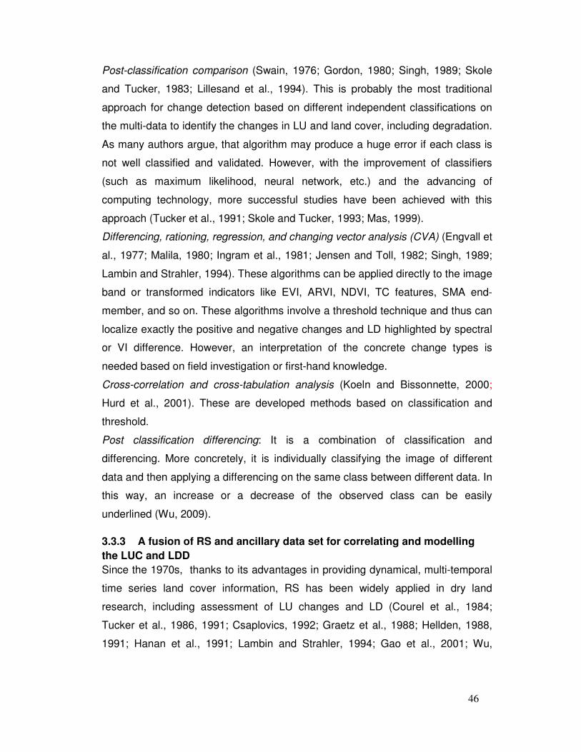
46
Post-classification comparison (Swain, 1976; Gordon, 1980; Singh, 1989; Skole
and Tucker, 1983; Lillesand et al., 1994). This is probably the most traditional
approach for change detection based on different independent classifications on
the multi-data to identify the changes in LU and land cover, including degradation.
As many authors argue, that algorithm may produce a huge error if each class is
not well classified and validated. However, with the improvement of classifiers
(such as maximum likelihood, neural network, etc.) and the advancing of
computing technology, more successful studies have been achieved with this
approach (Tucker et al., 1991; Skole and Tucker, 1993; Mas, 1999).
Differencing, rationing, regression, and changing vector analysis (CVA) (Engvall et
al., 1977; Malila, 1980; Ingram et al., 1981; Jensen and Toll, 1982; Singh, 1989;
Lambin and Strahler, 1994). These algorithms can be applied directly to the image
band or transformed indicators like EVI, ARVI, NDVI, TC features, SMA end-
member, and so on. These algorithms involve a threshold technique and thus can
localize exactly the positive and negative changes and LD highlighted by spectral
or VI difference. However, an interpretation of the concrete change types is
needed based on field investigation or first-hand knowledge.
Cross-correlation and cross-tabulation analysis (Koeln and Bissonnette, 2000;
Hurd et al., 2001). These are developed methods based on classification and
threshold.
Post classification differencing: It is a combination of classification and
differencing. More concretely, it is individually classifying the image of different
data and then applying a differencing on the same class between different data. In
this way, an increase or a decrease of the observed class can be easily
underlined (Wu, 2009).
3.3.3 A fusion of RS and ancillary data set for correlating and modelling
the LUC and LDD
Since the 1970s, thanks to its advantages in providing dynamical, multi-temporal
time series land cover information, RS has been widely applied in dry land
research, including assessment of LU changes and LD (Courel et al., 1984;
Tucker et al., 1986, 1991; Csaplovics, 1992; Graetz et al., 1988; Hellden, 1988,
1991; Hanan et al., 1991; Lambin and Strahler, 1994; Gao et al., 2001; Wu,
47
2003a-c and 2004; Wu et al., 2002 and 2005). For instance spatiotemporal data of
LU and LDD could be integrated with different time series data, such as climatic,
socioeconomic, and demographic data, for making correlations and models for the
analysis and prediction of these parameters.
48
Chapter Four
Description of Study Area and Methodology
The chapter describes in details the study area and the methodology followed for
achieving the study’s objectives. The study area description included the Sudan
after secession of its the southern part, White State and the locality of Elgeteina
(the study area).
4.1 Description of study area
4.1.1 The Sudan
4.1.1.1 Location
The referendum in July 2011 led to the separation of southern Sudan as a
country; consequently, the Sudan’s new area is located at latitude 8°45’’ and
23°8’’ N and longitude 21°49’ and 38°34’’ its area has become about 1, 882,000
km2, bounding on the east by the Red Sea and on other sides by seven instead of
nine Africa countries; Eritrea and Ethiopia to the East; Southern Sudan in the
South; the Central Africa Republic and Chad to the West; and Libya and Egypt to
the North (Elsadig, 2011). It is divided administratively into 17 States: Khartoum,
White Nile, Blue Nile, Northern Kordufan, Northern Darfur, Blue Nile, Kassala, El
Gadarif, Northern, River Nile, Red Sea, El Gezira and Sinnar, Southern Kordufan,
Western Darfur, Eastern Darfur, and Central Darfur State (FAO, 2012) (Figure
(4.1)). The total population number amounts to approximately 39,187 million,
according to an estimation of last census 2008–2009 (Central Bureau of Statistics,
2009), and it has become a 33 million (Elsadig, 2011). People practice different
activities, such as agriculture, mining, trade, and different free works, but the
majority of them practice agriculture.
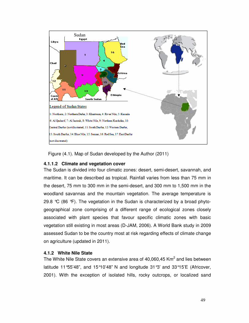
49
Figure (4.1). Map of Sudan developed by the Author (2011)
4.1.1.2 Climate and vegetation cover
The Sudan is divided into four climatic zones: desert, semi-desert, savannah, and
maritime. It can be described as tropical. Rainfall varies from less than 75 mm in
the desert, 75 mm to 300 mm in the semi-desert, and 300 mm to 1,500 mm in the
woodland savannas and the mountain vegetation. The average temperature is
29.8 °C (86 °F). The vegetation in the Sudan is characterized by a broad phyto-
geographical zone comprising of a different range of ecological zones closely
associated with plant species that favour specific climatic zones with basic
vegetation still existing in most areas (D-JAM, 2006). A World Bank study in 2009
assessed Sudan to be the country most at risk regarding effects of climate change
on agriculture (updated in 2011).
4.1.2 White Nile State
The White Nile State covers an extensive area of 40,060,45 Km2 and lies between
latitude 11°55’48”, and 15°10’48” N and longitude 31°3’ and 33°15’E (Africover,
2001). With the exception of isolated hills, rocky outcrops, or localized sand
Sudan
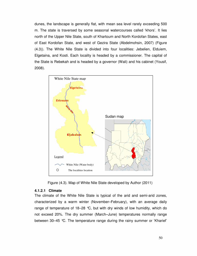
50
dunes, the landscape is generally flat, with mean sea level rarely exceeding 500
m. The state is traversed by some seasonal watercourses called ‘khors’. It lies
north of the Upper Nile State, south of Khartoum and North Kordofan States, east
of East Kordofan State, and west of Gezira State (Abdelmohsin, 2007) (Figure
(4.3)). The White Nile State is divided into four localities: Jebelien, Elduiem,
Elgetaina, and Kosti. Each locality is headed by a commissioner. The capital of
the State is Rebekah and is headed by a governor (Wali) and his cabinet (Yousif,
2008).
Sudan map
Figure (4.3). Map of White Nile State developed by Author (2011)
4.1.2.1 Climate
The climate of the White Nile State is typical of the arid and semi-arid zones,
characterized by a warm winter (November–February), with an average daily
range of temperature of 18–28 °C, but with dry winds of low humidity, which do
not exceed 20%. The dry summer (March–June) temperatures normally range
between 30–45 °C. The temperature range during the rainy summer or ‘Kharief’
White Nile State map
White Nile (Water body)
The localities location
Legend
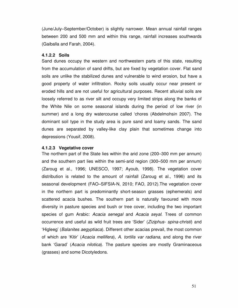
51
(June/July–September/October) is slightly narrower. Mean annual rainfall ranges
between 200 and 500 mm and within this range, rainfall increases southwards
(Gaiballa and Farah, 2004).
4.1.2.2 Soils
Sand dunes occupy the western and northwestern parts of this state, resulting
from the accumulation of sand drifts, but are fixed by vegetation cover. Flat sand
soils are unlike the stabilized dunes and vulnerable to wind erosion, but have a
good property of water infiltration. Rocky soils usually occur near present or
eroded hills and are not useful for agricultural purposes. Recent alluvial soils are
loosely referred to as river silt and occupy very limited strips along the banks of
the White Nile on some seasonal islands during the period of low river (in
summer) and a long dry watercourse called ‘chores (Abdelmohsin 2007). The
dominant soil type in the study area is pure sand and loamy sands. The sand
dunes are separated by valley-like clay plain that sometimes change into
depressions (Yousif, 2008).
4.1.2.3 Vegetative cover
The northern part of the State lies within the arid zone (200–300 mm per annum)
and the southern part lies within the semi-arid region (300–500 mm per annum)
(Zaroug et al., 1996; UNESCO, 1997; Ayoub, 1998). The vegetation cover
distribution is related to the amount of rainfall (Zaroug et al., 1996) and its
seasonal development (FAO–SIFSIA-N, 2010; FAO, 2012).The vegetation cover
in the northern part is predominantly short-season grasses (ephemerals) and
scattered acacia bushes. The southern part is naturally favoured with more
diversity in pasture species and bush or tree cover, including the two important
species of gum Arabic: Acacia senegal and Acacia seyal. Trees of common
occurrence and useful as wild fruit trees are ‘Sider’ (Ziziphus- spina-christi) and
‘Higleeg’ (Balanites aegyptiaca). Different other acacias prevail, the most common
of which are ‘Kitir’ (Acacia mellifera), A. tortilis var radiana, and along the river
bank ‘Garad’ (Acacia nilotica). The pasture species are mostly Graminaceous
(grasses) and some Dicotyledons.
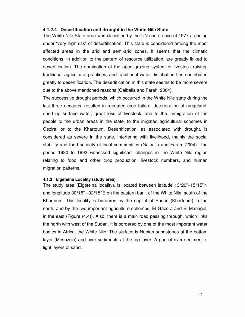
52
4.1.2.4 Desertification and drought in the White Nile State
The White Nile State area was classified by the UN conference of 1977 as being
under “very high risk” of desertification. This state is considered among the most
affected areas in the arid and semi-arid zones. It seems that the climatic
conditions, in addition to the pattern of resource utilization, are greatly linked to
desertification. The domination of the open grazing system of livestock raising,
traditional agricultural practices, and traditional water distribution has contributed
greatly to desertification. The desertification in this state seems to be more severe
due to the above mentioned reasons (Gaiballa and Farah, 2004).
The successive drought periods, which occurred in the White Nile state during the
last three decades, resulted in repeated crop failure, deterioration of rangeland,
dried up surface water, great loss of livestock, and to the immigration of the
people to the urban areas in the state, to the irrigated agricultural schemes in
Gezira, or to the Khartoum. Desertification, as associated with drought, is
considered as severe in the state, interfering with livelihood, mainly the social
stability and food security of local communities (Gaiballa and Farah, 2004). The
period 1980 to 1992 witnessed significant changes in the White Nile region
relating to food and other crop production, livestock numbers, and human
migration patterns.
4.1.3 Elgeteina Locality (study area)
The study area (Elgeteina locality), is located between latitude 13°20”–15°15”′N
and longitude 30°15” –32°15”′E on the eastern bank of the White Nile, south of the
Khartoum. This locality is bordered by the capital of Sudan (Khartoum) in the
north, and by the two important agriculture schemes, El Gazera and El Managel,
in the east (Figure (4.4)). Also, there is a main road passing through, which links
the north with west of the Sudan. It is bordered by one of the most important water
bodies in Africa, the White Nile. The surface is Nubian sandstones at the bottom
layer (Mesozoic) and river sediments at the top layer. A part of river sediment is
light layers of sand.
53
White Nile State Map
Source: Google Earth (2003)
Figure (4.4). Map of study area (Elgeteina Locality) developed by the Author (2011) The region lies between the semi-desert and Acacia desert shrubs region and the
rains range between 32 and 192 cm/year (Figure (4.5)). The period of drought
extends to 8 months, and the amount of rainfall decreases gradually towards the
north. There are two ecological regions: the semi desert and low rainfall savanna.
Figure (4.5). Rate of rainfall in the study area (Source: Sudan’s General Authority
of Meteorology (2008))
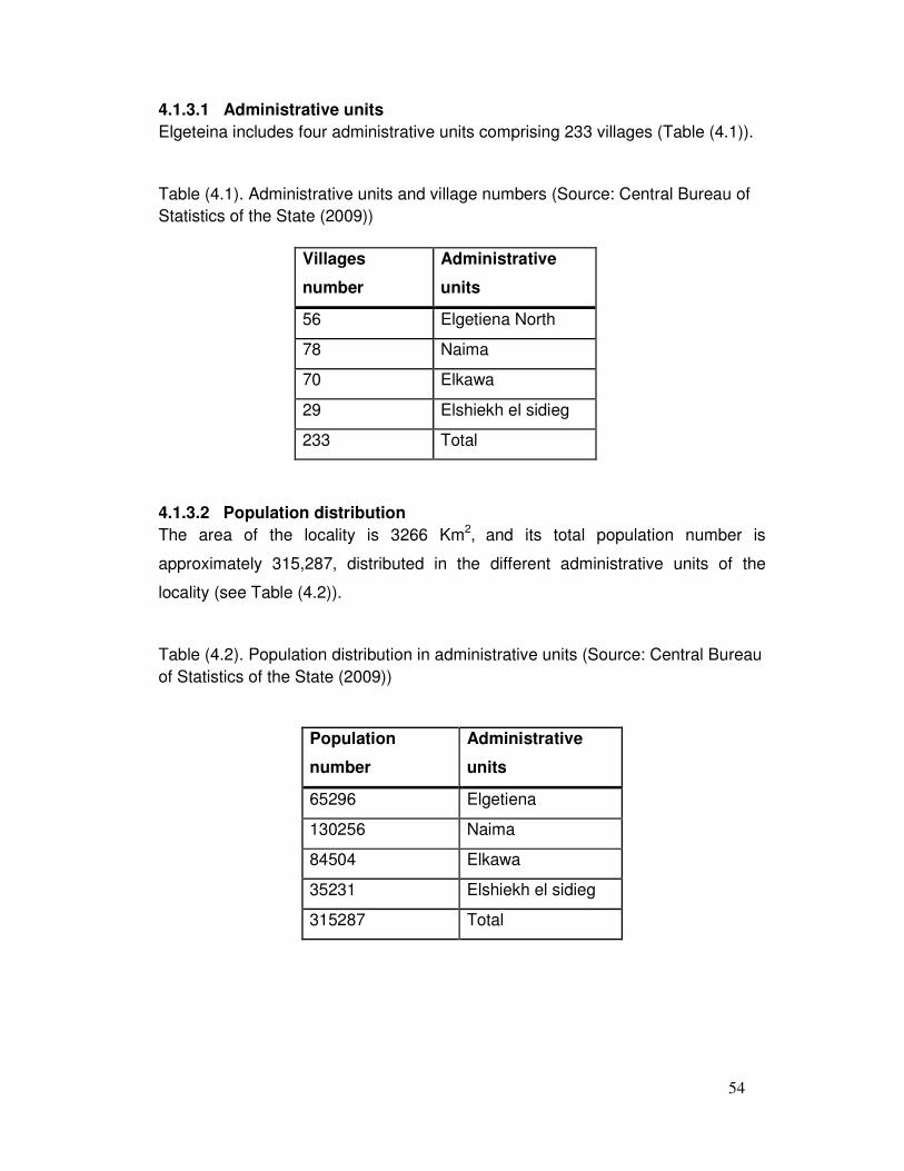
54
4.1.3.1 Administrative units
Elgeteina includes four administrative units comprising 233 villages (Table (4.1)).
Table (4.1). Administrative units and village numbers (Source: Central Bureau of Statistics of the State (2009))
Villages
number
Administrative
units
56 Elgetiena North
78 Naima
70 Elkawa
29 Elshiekh el sidieg
233 Total
4.1.3.2 Population distribution
The area of the locality is 3266 Km2, and its total population number is
approximately 315,287, distributed in the different administrative units of the
locality (see Table (4.2)).
Table (4.2). Population distribution in administrative units (Source: Central Bureau of Statistics of the State (2009))
Population
number
Administrative
units
65296 Elgetiena
130256 Naima
84504 Elkawa
35231 Elshiekh el sidieg
315287 Total
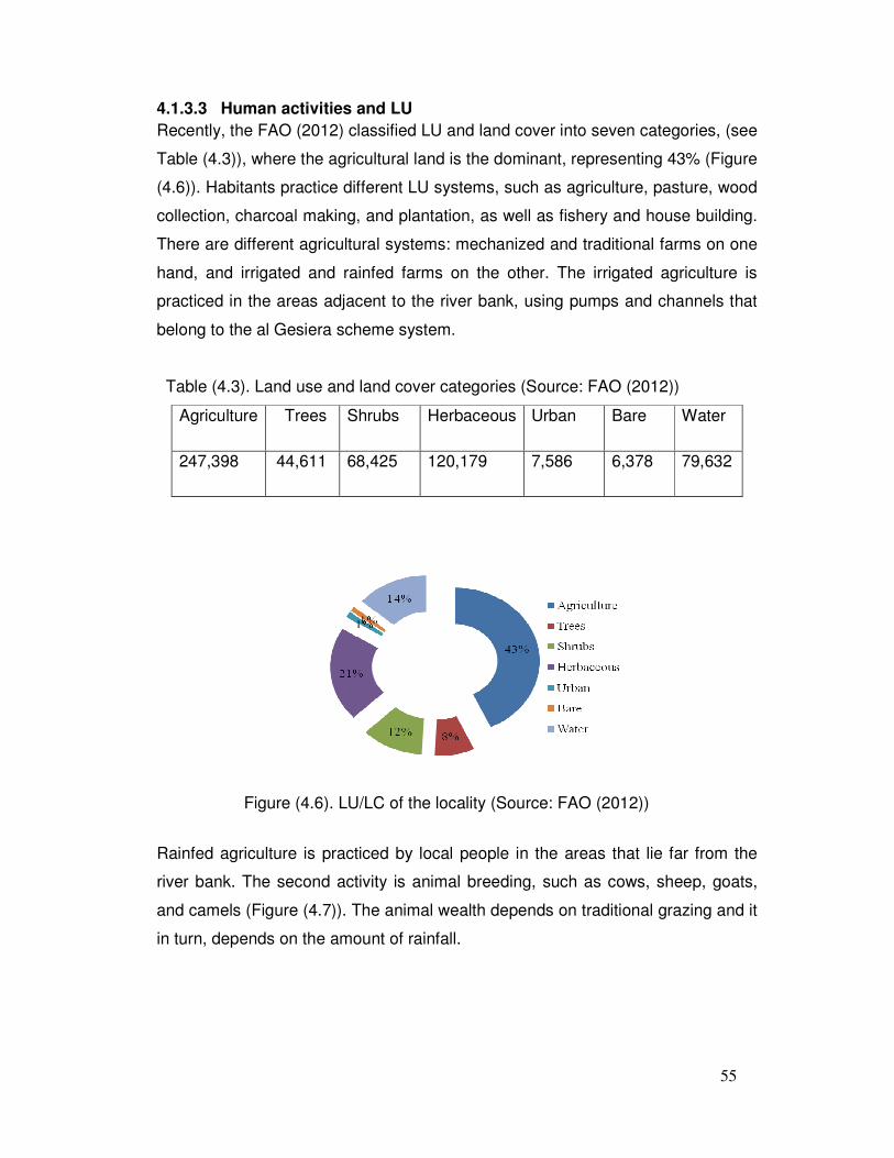
55
4.1.3.3 Human activities and LU
Recently, the FAO (2012) classified LU and land cover into seven categories, (see
Table (4.3)), where the agricultural land is the dominant, representing 43% (Figure
(4.6)). Habitants practice different LU systems, such as agriculture, pasture, wood
collection, charcoal making, and plantation, as well as fishery and house building.
There are different agricultural systems: mechanized and traditional farms on one
hand, and irrigated and rainfed farms on the other. The irrigated agriculture is
practiced in the areas adjacent to the river bank, using pumps and channels that
belong to the al Gesiera scheme system.
Table (4.3). Land use and land cover categories (Source: FAO (2012))
Agriculture Trees Shrubs Herbaceous Urban Bare Water
247,398 44,611 68,425 120,179 7,586 6,378 79,632
Figure (4.6). LU/LC of the locality (Source: FAO (2012))
Rainfed agriculture is practiced by local people in the areas that lie far from the
river bank. The second activity is animal breeding, such as cows, sheep, goats,
and camels (Figure (4.7)). The animal wealth depends on traditional grazing and it
in turn, depends on the amount of rainfall.
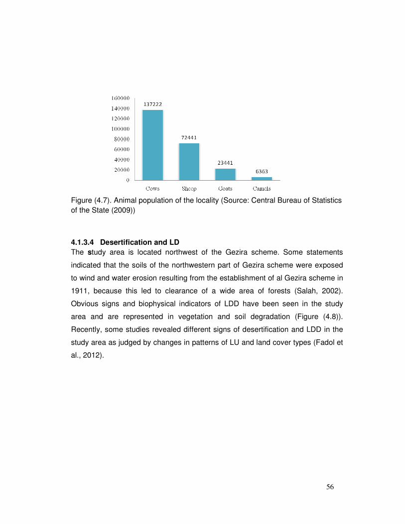
56
Figure (4.7). Animal population of the locality (Source: Central Bureau of Statistics of the State (2009))
4.1.3.4 Desertification and LD
The study area is located northwest of the Gezira scheme. Some statements
indicated that the soils of the northwestern part of Gezira scheme were exposed
to wind and water erosion resulting from the establishment of al Gezira scheme in
1911, because this led to clearance of a wide area of forests (Salah, 2002).
Obvious signs and biophysical indicators of LDD have been seen in the study
area and are represented in vegetation and soil degradation (Figure (4.8)).
Recently, some studies revealed different signs of desertification and LDD in the
study area as judged by changes in patterns of LU and land cover types (Fadol et
al., 2012).
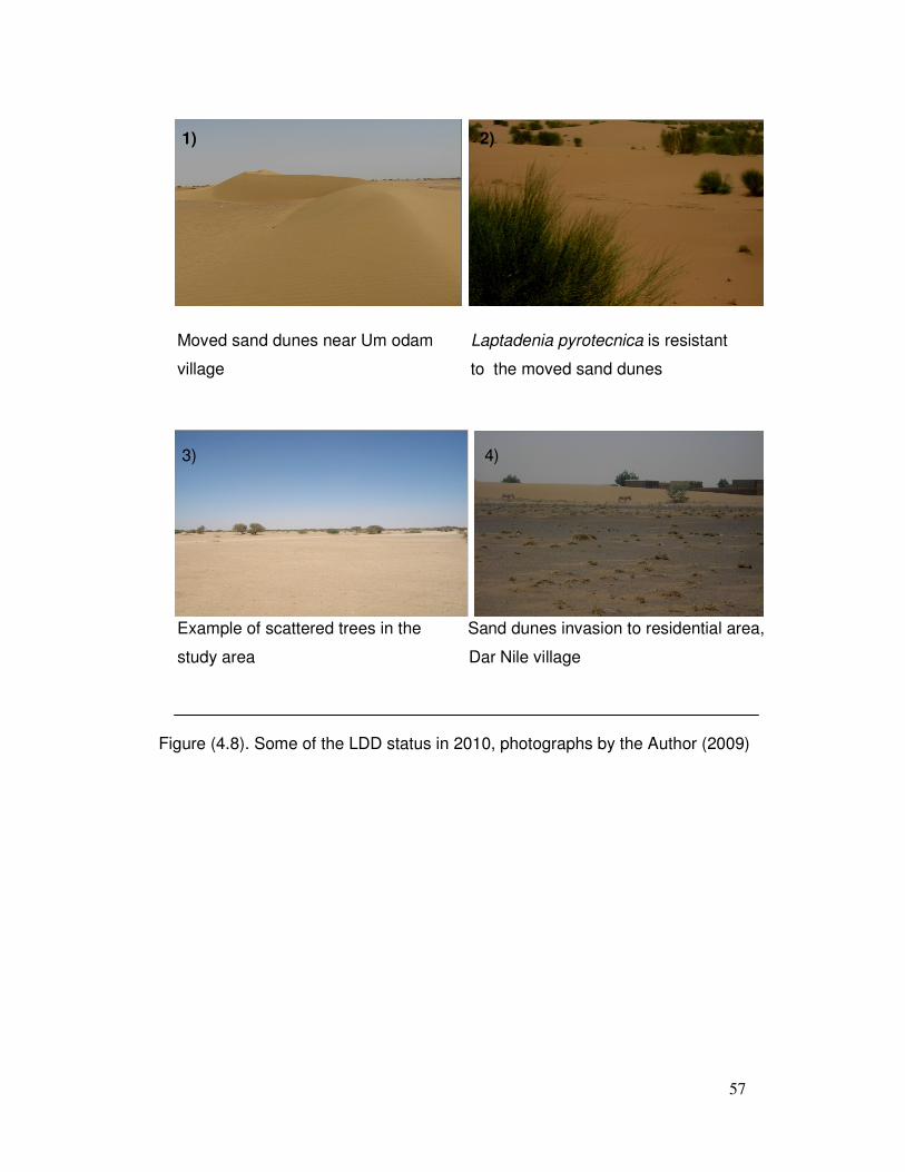
57
1) 2)
Moved sand dunes near Um odam Laptadenia pyrotecnica is resistant
village to the moved sand dunes
3) 4)
Example of scattered trees in the Sand dunes invasion to residential area,
study area Dar Nile village
Figure (4.8). Some of the LDD status in 2010, photographs by the Author (2009)
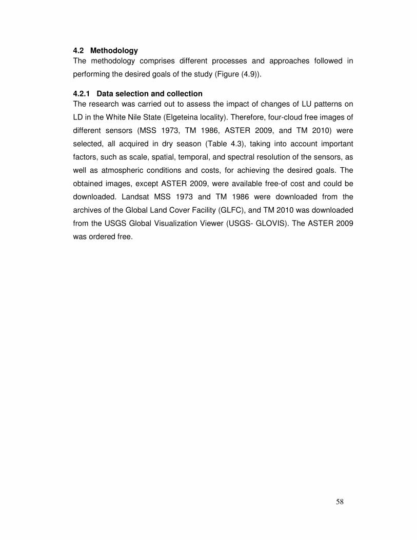
58
4.2 Methodology
The methodology comprises different processes and approaches followed in
performing the desired goals of the study (Figure (4.9)).
4.2.1 Data selection and collection
The research was carried out to assess the impact of changes of LU patterns on
LD in the White Nile State (Elgeteina locality). Therefore, four-cloud free images of
different sensors (MSS 1973, TM 1986, ASTER 2009, and TM 2010) were
selected, all acquired in dry season (Table 4.3), taking into account important
factors, such as scale, spatial, temporal, and spectral resolution of the sensors, as
well as atmospheric conditions and costs, for achieving the desired goals. The
obtained images, except ASTER 2009, were available free-of cost and could be
downloaded. Landsat MSS 1973 and TM 1986 were downloaded from the
archives of the Global Land Cover Facility (GLFC), and TM 2010 was downloaded
from the USGS Global Visualization Viewer (USGS- GLOVIS). The ASTER 2009
was ordered free.
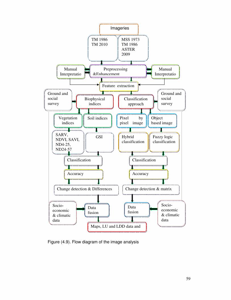
59
Soil indices
TM 1986
TM 2010
MSS 1973
TM 1986
ASTER
2009
Preprocessing
&Enhancement
Feature extraction
extraction
Biophysical
indices
approach
Manual
Interpretatio
Manual
Interpretatio
Classification
approach
Vegetation
indices
Pixel by
pixel image
Object
based image
Ground and
social
survey
Socio-
economic
& climatic
data
Hybrid
classification
Fuzzy logic
classification
GSI SARV,
NDVI, SAVI,
ND4-25,
ND24-57
Classification
output
Change detection & matrix Change detection & Differences
Accuracy
assessment
Classification
output
Accuracy
assessment
Data
fusion
Data
fusion
Maps, LU and LDD data and
others
Socio-
economic
& climatic
data
Ground and
social
survey
Imageries
Figure (4.9). Flow diagram of the image analysis
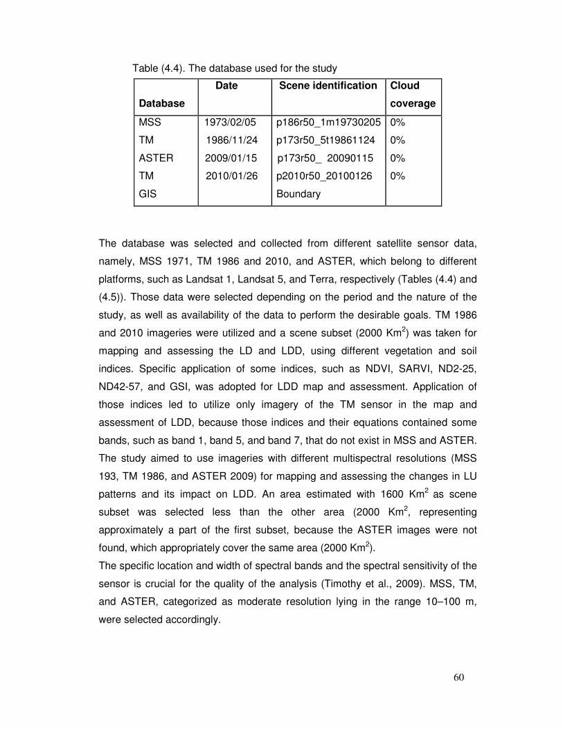
60
Table (4.4). The database used for the study
The database was selected and collected from different satellite sensor data,
namely, MSS 1971, TM 1986 and 2010, and ASTER, which belong to different
platforms, such as Landsat 1, Landsat 5, and Terra, respectively (Tables (4.4) and
(4.5)). Those data were selected depending on the period and the nature of the
study, as well as availability of the data to perform the desirable goals. TM 1986
and 2010 imageries were utilized and a scene subset (2000 Km2) was taken for
mapping and assessing the LD and LDD, using different vegetation and soil
indices. Specific application of some indices, such as NDVI, SARVI, ND2-25,
ND42-57, and GSI, was adopted for LDD map and assessment. Application of
those indices led to utilize only imagery of the TM sensor in the map and
assessment of LDD, because those indices and their equations contained some
bands, such as band 1, band 5, and band 7, that do not exist in MSS and ASTER.
The study aimed to use imageries with different multispectral resolutions (MSS
193, TM 1986, and ASTER 2009) for mapping and assessing the changes in LU
patterns and its impact on LDD. An area estimated with 1600 Km2 as scene
subset was selected less than the other area (2000 Km2, representing
approximately a part of the first subset, because the ASTER images were not
found, which appropriately cover the same area (2000 Km2).
The specific location and width of spectral bands and the spectral sensitivity of the
sensor is crucial for the quality of the analysis (Timothy et al., 2009). MSS, TM,
and ASTER, categorized as moderate resolution lying in the range 10–100 m,
were selected accordingly.
Database
Date Scene identification Cloud
coverage
MSS
TM
ASTER
TM
GIS
1973/02/05
1986/11/24
2009/01/15
2010/01/26
p186r50_1m19730205
p173r50_5t19861124
p173r50_ 20090115
p2010r50_20100126
Boundary
0%
0%
0%
0%
61
Table (4.5). The characteristics of the selected database used in the research
MSS, TM, and ASTER data cover an area of about 185 × 185 and 60 × 60 Km,
respectively, and two types of sub-scenes were selected: one sub-scene for
assessing LD and the other for mapping and assessing effects of LU changes on
LD, covering about 2000 km2, and 1600 km2, respectively, including a long part of
the White Nile in the Elgeteina locality (Figure (4.10)).
Instrument Properties
MSS
TM
ASTER
Landsat Landsat1 Landsat5 Terra
Spectral bands (µm)
4 bands 1. 0.5–0.6 (green) 2. 0.6–0.7 (red) 3.0.7–0-0 (near-infrared) 4.0.8–1.1(mid-infrared)
7 bands 1.0.45–0.52 (blue) 2.0.52–0.60 (green) 3. 0.63–0.69 (red) 4. 0.76–0.90 (near-infrared) 5. 1.55–1.75 (mid-infrared) 6. 10.4–12.5 (thermal) 7. 2.08–2.35 (mid-infrared)
14 bands (3 bands= NIR), (6b=SWIR) & (5b=TIR) 3b range = 1.0.52–0.60 (green) 2.0.63–0.69 (red) 3.0.76–0.86 (near-infrared)
Ground resolution
79 × 79m 30 × 30m 15 ×15m
Dynamic range (bit)
7 bits 8 bits 8 bits
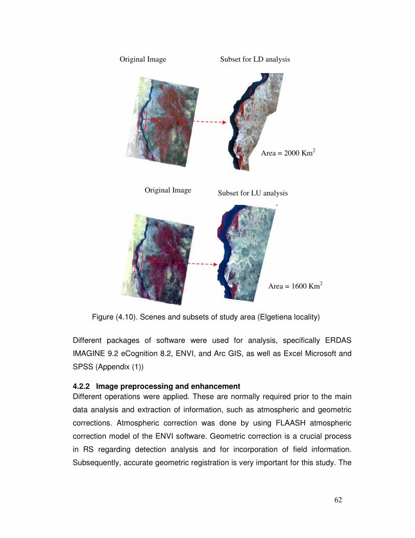
62
Figure (4.10). Scenes and subsets of study area (Elgetiena locality)
Different packages of software were used for analysis, specifically ERDAS
IMAGINE 9.2 eCognition 8.2, ENVI, and Arc GIS, as well as Excel Microsoft and
SPSS (Appendix (1))
4.2.2 Image preprocessing and enhancement
Different operations were applied. These are normally required prior to the main
data analysis and extraction of information, such as atmospheric and geometric
corrections. Atmospheric correction was done by using FLAASH atmospheric
correction model of the ENVI software. Geometric correction is a crucial process
in RS regarding detection analysis and for incorporation of field information.
Subsequently, accurate geometric registration is very important for this study. The
Subset for LD analysis Original Image
Area = 2000 Km2
Area = 1600 Km2
Original Image Subset for LU analysis
63
imagery used in this research is already geometrically corrected at the LG1 level
for Landsat imagery (MSS, TM) and at the LB1 level of ASTER image. Moreover,
the research area characterized by relatively flat terrain, and the atmospheric
condition at the time of acquisition was very good, ensuring more satellite orbit
and good imaging quality. Those factors make the geometric correction not
necessary in this research. However, the registration image to image is needed
precisely for the comparison. Therefore, the study carried out co-registration,
where 21 GCPs for each image were distributed properly, and a nearest
neighbour resampling method was applied by the image-to-image registration
technique in the ERDAS Imagine. The root mean square error (RMSE) ranged
from 0.1–0.3 pixel of each registration procedure image, revealing a higher
sufficient precision of rectification.
To display and record data more effectively for subsequent visual interpretation,
image enhancement was done for increasing the visual distinctions between
features in a scene, doing different procedures to manipulate the contrast and
spatial features by using contrast stretching of an image.
4.2.3 Approaches of image processing for deriving information
Different approaches for image processing to derive information for assessing
LDD and LU impacts were taken as follows:
4.2.3.1 Visual image interpretation
Visual image interpretation was done before achieving the field survey for
interpreting the features of the study area, determining the targets, and setting a
plan of work for facilitating the survey task. The visual image interpretation was
done in the research area by observing the variation of the pattern, shape, texture,
association, and size.
4.2.3.2 The biophysical indices approach
The study attempted to integrate vegetation index (VI) and soil degradation (SI),
ground truth, and laboratory analysis to assess LDD to increase the accuracy of
the information for assessing LDD in semi-arid regions:
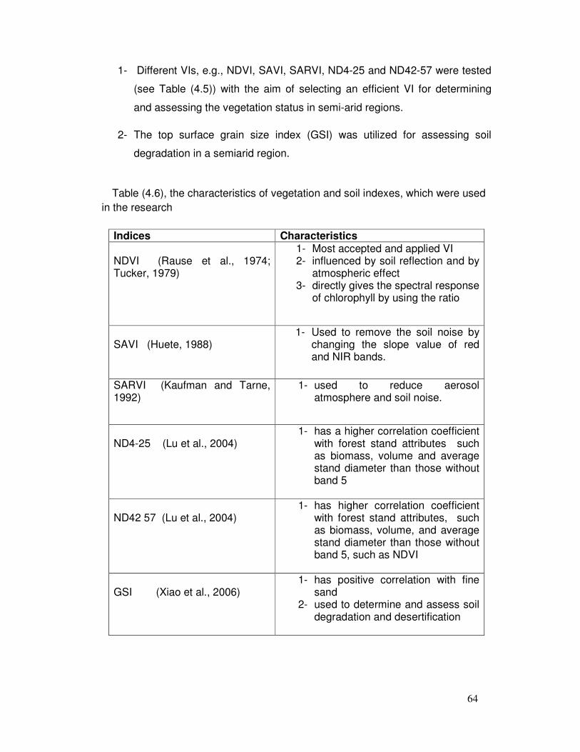
64
1- Different VIs, e.g., NDVI, SAVI, SARVI, ND4-25 and ND42-57 were tested
(see Table (4.5)) with the aim of selecting an efficient VI for determining
and assessing the vegetation status in semi-arid regions.
2- The top surface grain size index (GSI) was utilized for assessing soil
degradation in a semiarid region.
Table (4.6), the characteristics of vegetation and soil indexes, which were used in the research
Indices Characteristics NDVI (Rause et al., 1974; Tucker, 1979)
1- Most accepted and applied VI 2- influenced by soil reflection and by
atmospheric effect 3- directly gives the spectral response
of chlorophyll by using the ratio
SAVI (Huete, 1988)
1- Used to remove the soil noise by changing the slope value of red and NIR bands.
SARVI (Kaufman and Tarne, 1992)
1- used to reduce aerosol atmosphere and soil noise.
ND4-25 (Lu et al., 2004)
1- has a higher correlation coefficient with forest stand attributes such as biomass, volume and average stand diameter than those without band 5
ND42 57 (Lu et al., 2004)
1- has higher correlation coefficient with forest stand attributes, such as biomass, volume, and average stand diameter than those without band 5, such as NDVI
GSI (Xiao et al., 2006)
1- has positive correlation with fine sand
2- used to determine and assess soil degradation and desertification
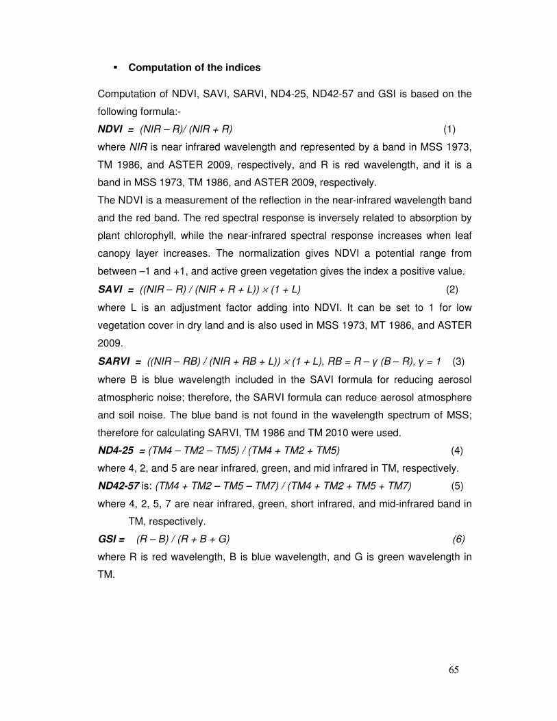
65
� Computation of the indices
Computation of NDVI, SAVI, SARVI, ND4-25, ND42-57 and GSI is based on the
following formula:-
NDVI = (NIR – R)/ (NIR + R) (1)
where NIR is near infrared wavelength and represented by a band in MSS 1973,
TM 1986, and ASTER 2009, respectively, and R is red wavelength, and it is a
band in MSS 1973, TM 1986, and ASTER 2009, respectively.
The NDVI is a measurement of the reflection in the near-infrared wavelength band
and the red band. The red spectral response is inversely related to absorption by
plant chlorophyll, while the near-infrared spectral response increases when leaf
canopy layer increases. The normalization gives NDVI a potential range from
between –1 and +1, and active green vegetation gives the index a positive value.
SAVI = ((NIR – R) / (NIR + R + L)) × (1 + L) (2)
where L is an adjustment factor adding into NDVI. It can be set to 1 for low
vegetation cover in dry land and is also used in MSS 1973, MT 1986, and ASTER
2009.
SARVI = ((NIR – RB) / (NIR + RB + L)) × (1 + L), RB = R – γ (B – R), γ = 1 (3)
where B is blue wavelength included in the SAVI formula for reducing aerosol
atmospheric noise; therefore, the SARVI formula can reduce aerosol atmosphere
and soil noise. The blue band is not found in the wavelength spectrum of MSS;
therefore for calculating SARVI, TM 1986 and TM 2010 were used.
ND4-25 = (TM4 – TM2 – TM5) / (TM4 + TM2 + TM5) (4)
where 4, 2, and 5 are near infrared, green, and mid infrared in TM, respectively.
ND42-57 is: (TM4 + TM2 – TM5 – TM7) / (TM4 + TM2 + TM5 + TM7) (5)
where 4, 2, 5, 7 are near infrared, green, short infrared, and mid-infrared band in
TM, respectively.
GSI = (R – B) / (R + B + G) (6)
where R is red wavelength, B is blue wavelength, and G is green wavelength in
TM.
66
� Ground survey and data collection
In general, two field surveys were carried out in the dry season during the period
of the research (in February up to May 2009 and at the end of March up to the
beginning of June 2010), for collecting and verifying the data regarding the VIs
and Sis. Determination of different levels of vegetation according to the values of
NDVI, SAVI, and SARVI, (that range –1 and +1) as well as ND4-25 and ND42-57,
was done properly for identifying the vegetation cover status as a biophysical
indicator for vegetation degradation. With regard to the GSI, different field work
was done: first the determination of sand and sand dune accumulation,
considered a serious biophysical indicator to the soil degradation, was based on
GSI values, where the survey could determine the different types of soil properly.
The ground positioning system widely was used for the above vegetation and soil
observation survey.
Data analysis
After ground survey and collecting information concerning the vegetation and soil
status corresponding to values of VIs (NDVI, SAVI, SARVI, ND4-25, and ND42-
57) and SI (GSI) of the imagery, statistical parameters were computed (mean,
standard deviation, total, maximum, and minimum) using ERDAS IMAGINE 9.2
and Arc GIS software.
� Change detection of VIs and SIs
Image differencing was calculated for the VIs and SIs to estimate the change
detection for assessing the spatiotemporal status of the vegetation and soil
degradation separately. Image differencing is a simple way to identify the changes
between two images (that are properly calibrated and rectified) by computing the
pixel-to-pixel difference in the single bands or derived indices (Chuvieco and
Heute, 2010). That was suitable for comparison between VI and SI, whereas the
subtraction for VIs and SIs images was done for TM 1986 and 2010, where TM
2010 was subtracted from TM 1986.
Differencing index = Dlt2 – Dlt1 + C
where Dlt2 and Dlt1 are the values of the two periods being compared, and C is a
constant value added to the modified image difference to avoid negative numbers.
67
4.2.3.3 Pixel based- and object-based image analysis approach
PBIA and OBIA were used to map and assess the impact of spatiotemporal
changes in LU patterns on land degradation (vegetation and soil) with the aim of
assessing the two methods in the accuracy and efficiency in performing the goals.
The analysis was applied on MSS 1973, TM 1986, and ASTER 2009 to derive
information.
4.2.3.3.1 Pixel based image analysis
Hybrid classification was used, one of the PBIA approaches, and it is a combined
method between unsupervised and supervised classification:
4.2.3.3.1.1 Hybrid classification
Firstly, an unsupervised classification was performed, and the result interpreted
using ground truth knowledge derived from two ground surveys done in 2009 and
2010. Finally, the original image was reclassified using a supervised classification
with the aid of the statistics of the unsupervised classification as training
knowledge (Figure (4.11)). The combination method (hybrid) provides more
objective and reliable results (Liu and Mason, 2009).
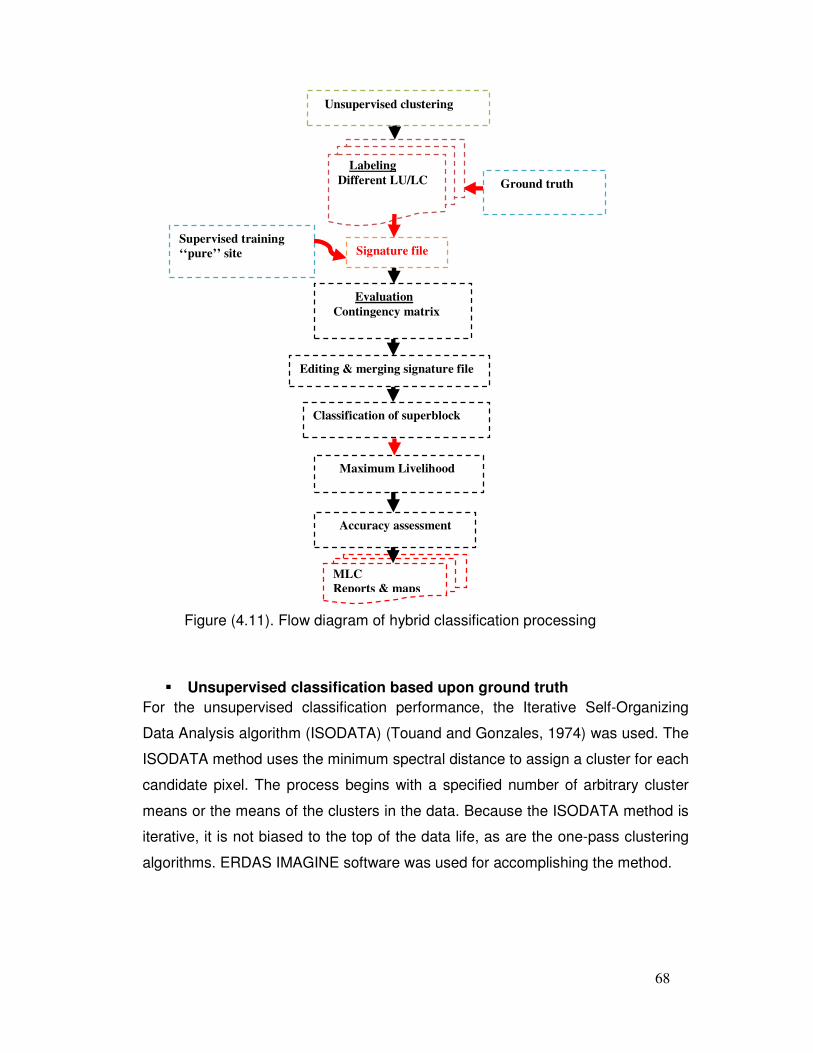
68
Figure (4.11). Flow diagram of hybrid classification processing
� Unsupervised classification based upon ground truth
For the unsupervised classification performance, the Iterative Self-Organizing
Data Analysis algorithm (ISODATA) (Touand and Gonzales, 1974) was used. The
ISODATA method uses the minimum spectral distance to assign a cluster for each
candidate pixel. The process begins with a specified number of arbitrary cluster
means or the means of the clusters in the data. Because the ISODATA method is
iterative, it is not biased to the top of the data life, as are the one-pass clustering
algorithms. ERDAS IMAGINE software was used for accomplishing the method.
Unsupervised clustering
Labeling
Different LU/LC
Supervised training
‘‘pure’’ site Signature file
Editing & merging signature file
Evaluation
Contingency matrix
Classification of superblock
Accuracy assessment
MLC
Reports & maps
Ground truth
Maximum Livelihood
69
Clustering parameters for performing ISODATA were set as follows: the number
of classes was 7, the maximum iteration was 24, and convergence threshold was
0.950.
After the classification was performed, the fieldwork knowledge was used in
interpreting the unsupervised classification results.
� Supervised classification based upon unsupervised classification
The supervised classification of an image generally depends on previous
knowledge of a study area acquired from external sources of fieldwork. In this
research, it depended on the statistics of the above unsupervised classification.
Then the maximum likelihood algorithm was used after collection of signatures
regarding classes of LU and LDD. LU and LDD were divided into seven classes.
4.2.3.3.2 Object-based image analysis
In OBIA, eCognition software 8.2 was used for analysing and deriving information.
OBIA includes two steps: segmentation and classification rules:
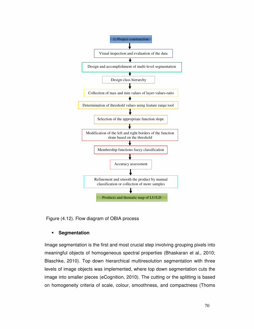
70
Figure (4.12). Flow diagram of OBIA process
� Segmentation
Image segmentation is the first and most crucial step involving grouping pixels into
meaningful objects of homogeneous spectral properties (Bhaskaran et al., 2010;
Blaschke, 2010). Top down hierarchical multiresolution segmentation with three
levels of image objects was implemented, where top down segmentation cuts the
image into smaller pieces (eCognition, 2010). The cutting or the splitting is based
on homogeneity criteria of scale, colour, smoothness, and compactness (Thoms
Accuracy assessment
Modification of the left and right borders of the function
slope based on the threshold
Membership functions fuzzy classification
1) Project construction
Selection of the appropriate function slope
Visual inspection and evaluation of the data
Design and accomplishment of multi-level segmentation
Design class hierarchy
Collection of max and min values of layer-values-ratio
Determination of threshold values using feature range tool
Refinement and smooth the product by manual
classification or collection of more samples
Products and thematic map of LU/LD
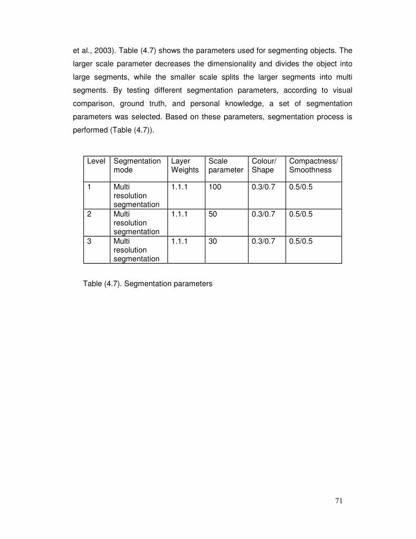
71
et al., 2003). Table (4.7) shows the parameters used for segmenting objects. The
larger scale parameter decreases the dimensionality and divides the object into
large segments, while the smaller scale splits the larger segments into multi
segments. By testing different segmentation parameters, according to visual
comparison, ground truth, and personal knowledge, a set of segmentation
parameters was selected. Based on these parameters, segmentation process is
performed (Table (4.7)).
Table (4.7). Segmentation parameters
Level Segmentation mode
Layer Weights
Scale parameter
Colour/ Shape
Compactness/ Smoothness
1 Multi resolution segmentation
1.1.1 100 0.3/0.7 0.5/0.5
2 Multi resolution segmentation
1.1.1 50 0.3/0.7 0.5/0.5
3 Multi resolution segmentation
1.1.1 30 0.3/0.7 0.5/0.5
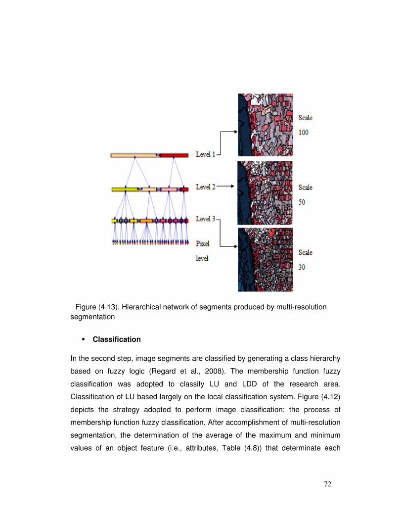
72
Figure (4.13). Hierarchical network of segments produced by multi-resolution segmentation
� Classification
In the second step, image segments are classified by generating a class hierarchy
based on fuzzy logic (Regard et al., 2008). The membership function fuzzy
classification was adopted to classify LU and LDD of the research area.
Classification of LU based largely on the local classification system. Figure (4.12)
depicts the strategy adopted to perform image classification: the process of
membership function fuzzy classification. After accomplishment of multi-resolution
segmentation, the determination of the average of the maximum and minimum
values of an object feature (i.e., attributes, Table (4.8)) that determinate each
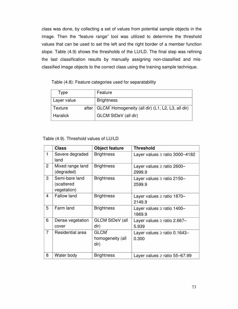
73
class was done, by collecting a set of values from potential sample objects in the
image. Then the “feature range” tool was utilized to determine the threshold
values that can be used to set the left and the right border of a member function
slope. Table (4.9) shows the thresholds of the LU/LD. The final step was refining
the last classification results by manually assigning non-classified and mis-
classified image objects to the correct class using the training sample technique.
Table (4.8): Feature categories used for separatability
Table (4.9). Threshold values of LU/LD
Type Feature
Layer value Brightness
Texture after
Haralick
GLCM* Homogeneity (all dir) (L1, L2, L3, all dir)
GLCM StDeV (all dir)
Class Object feature Threshold
1 Severe degraded land
Brightness Layer values ≥ ratio 3000–4182
2 Mixed range land (degraded)
Brightness Layer values ≥ ratio 2600–2999.9
3 Semi-bare land (scattered vegetation)
Brightness Layer values ≥ ratio 2150–2599.9
4 Fallow land Brightness Layer values ≥ ratio 1870–2149.9
5 Farm land Brightness Layer values ≥ ratio 1400–1869.9
6 Dense vegetation cover
GLCM StDeV (all dir)
Layer values ≥ ratio 2.667–5.939
7 Residential area GLCM*
homogeneity (all dir)
Layer values ≥ ratio 0.1643–0.300
8 Water body Brightness Layer values ≥ ratio 55–67.99
74
4.2.3.3.3 Assessment of classification performance
Accuracy assessment determines the quality of the information obtained from RS
data. The accuracy assessment of classification was applied for both methods
(PBIA and OBIA) by using an error matrix (sometimes called confusion matrix or
contingency table) (Card, 1982; Congalton, 1991). The error matrix is the most
common method of assessing the degree of accuracy (Mather, 2004) and has
been used widely in the classification accuracy assessment (e.g., Taruvinga,
2008; Pirie, 2009; Mararakanye et al., 2012). The error matrix is a square
containing rows and columns equal to the number of categories whose
classification accuracy is being assessed (Lillesand et al., 2008). The accuracy
assessment conducted based on the classification results for seven and eight LU
and LDD classes for PBIA-hyper classifier and OBIA-fuzzy classifier, respectively.
A total of 250 equalised random sample points (for each one of the two methods)
were generated using the ERDAS imagine accuracy assessment tool. The results
of the error matrix were interpreted using the producer’s accuracy, user’s
accuracy, overall classification accuracy, and the kappa coefficient statistics. The
overall classification accuracy summarises the producer’s and the user’s accuracy
and is the ratio between the numbers of samples correctly classified and the total
number of test samples. The user’s accuracy measures the errors of commission,
and the producer’s accuracy measures the errors of omission. The Kappa
coefficient of accuracy is the difference between the actual agreement in the error
matrix and the chance agreement (Persello & Bruzzone, 2010; Mararakanye et
al., 2012).
4.2.3.4 Change detection and matrix to estimate the changes in land use
and land degradation
Change detection was done in the period 1973–1986 and 1986–2009 using the
classified images of MSS and TM and TM and ASTER, respectively, to detect the
changes of LU and LDD that have occurred during those periods using the image
difference technique. Then the change detection matrix was performed to
determine the spatiotemporal effectiveness of changes of LU patterns on LDD.
75
4.2.3.5 Fusion of climatic, socioeconomic and remote sensing data
approach
The climatic, socioeconomic, and RS data were integrated to determine the
relationship between different factors, spatiotemporal changes of LU patterns, and
LDD to analyse the reasons behind the changes of LU patterns and its effect on
LDD and furthermore, to model LD influenced by LU/LCC, climatic variability, and
population growth.
The climatic data, including rainfall (RF), mean annual temperature (MT), wind
speed (WS), and relative humidity (RH) data for 1976 to 2009 were collected from
the Meteorological Authority of the Sudan. Socioeconomic data concerning social,
economical, cultural, and demographic data were collected through a
questionnaire and from the Central Bureau of Statistics of the State (Appendix 2).
The questionnaire is defined as a document containing the questions and other
types of items designed to solicit information appropriate for analysis (Babbie,
1990). In this study, the questionnaire was used to collect socioeconomic data to
analyse the impact of socioeconomic dimension on LU change and LDD in the
study area, where 100 respondents of the local populations were interviewed
directly. The respondents lived in 10 villages from the Elgeteina locality.
Different methods of analysis were taken for analysing, correlating, and modelling:
Pearson coefficient correlation analysis was used for analysing the relationship
between climate variability and LU/LCC, and the relationship between population
growth rates, using SPSS software.
Two and three-dimensional pie charts were applied for analysing the
socioeconomic data by using Microsoft Office Excel 2007.
Pearson coefficient correlation and multiple linear regression analysis were
applied in the processes for establishing a model of LD (vegetation and soil
degradation) influenced by LU patterns (classes), using SPSS software.
76
Chapter 5
Findings of Analysis of Multi Temporal and Spectral Imagery and Ancillary
Datasets for the LDD and LU Patterns in a Semi-Arid Area of Elgeteina
The chapter reviews the results from the analysis methods described in the
previous chapter. The results include the assessment of LDD by using appropriate
indices; assessment of the impact of the changes in LU on LDD by comparing
between pixel- and object-based approaches; modelling and predicting the impact
of LUC on LDD; and analysis of the causative factors of LUC and/or LDD in the
study area.
5.1 Assessment of LDD by using biophysical indices
The assessment of the LDD is based on two significant biophysical indicators: the
vegetation degradation and the soil degradation (sand dune accumulation and
movement). These two parameters have usually been mapped and estimated
from satellite imagery (Liu et al., 2002). The vegetation and soil indexes were
used for deriving information for both the vegetation and soil degradation.
5.1.1 Assessment of vegetation degradation by using appropriate
vegetation indices
� Appropriate vegetation index for the vegetation status indication:
The output for searching a competent vegetation index through testing five
different vegetation indices (NDVI, SAVI, SARVI, ND4-25, and ND42-57) to
assess the vegetation status in the semi-arid environment of Sudan based on the
visual interpretation of maps of the vegetation indices and their correspondence
with the actual vegetation cover in the field revealed that SARVI was slightly better
than the other indices for indicating the vegetation cover (Figure (5.1) and Table
(5.1)).
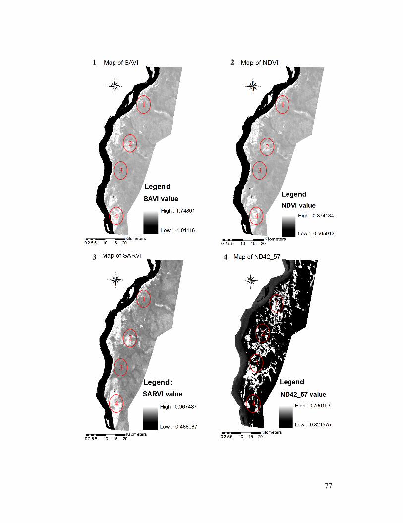
77
1
3 4
2
1
1 1
1
2
2 2
2
3 3
3 3
4
4 4
4
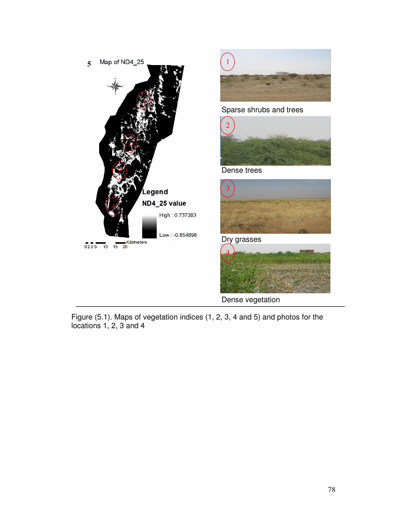
78
Sparse shrubs and trees Dense trees
Dry grasses
Dense vegetation
Figure (5.1). Maps of vegetation indices (1, 2, 3, 4 and 5) and photos for the locations 1, 2, 3 and 4
5 1
1
2
2
3
3
4
4
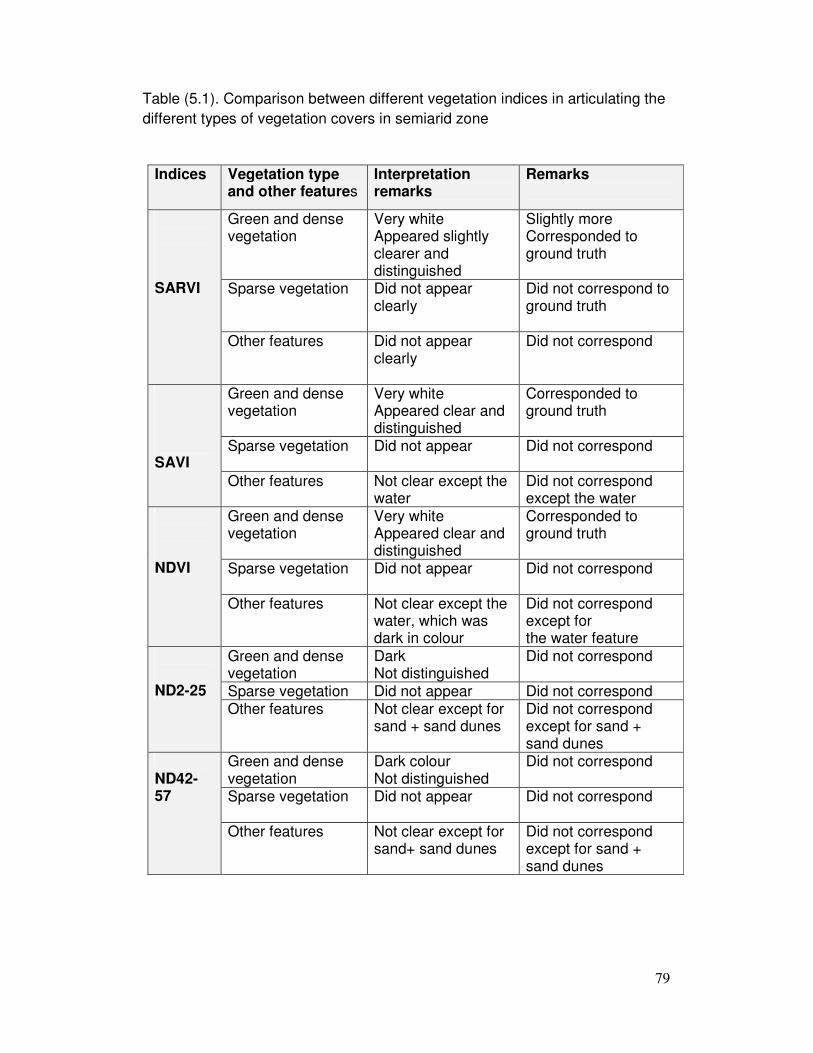
79
Table (5.1). Comparison between different vegetation indices in articulating the different types of vegetation covers in semiarid zone
Indices Vegetation type and other features
Interpretation remarks
Remarks
SARVI
Green and dense vegetation
Very white Appeared slightly clearer and distinguished
Slightly more Corresponded to ground truth
Sparse vegetation Did not appear clearly
Did not correspond to ground truth
Other features Did not appear clearly
Did not correspond
SAVI
Green and dense vegetation
Very white Appeared clear and distinguished
Corresponded to ground truth
Sparse vegetation Did not appear
Did not correspond
Other features Not clear except the water
Did not correspond except the water
NDVI
Green and dense vegetation
Very white Appeared clear and distinguished
Corresponded to ground truth
Sparse vegetation Did not appear Did not correspond
Other features Not clear except the water, which was dark in colour
Did not correspond except for the water feature
ND2-25
Green and dense vegetation
Dark Not distinguished
Did not correspond
Sparse vegetation Did not appear Did not correspond Other features Not clear except for
sand + sand dunes Did not correspond except for sand + sand dunes
ND42-57
Green and dense vegetation
Dark colour Not distinguished
Did not correspond
Sparse vegetation Did not appear
Did not correspond
Other features Not clear except for sand+ sand dunes
Did not correspond except for sand + sand dunes
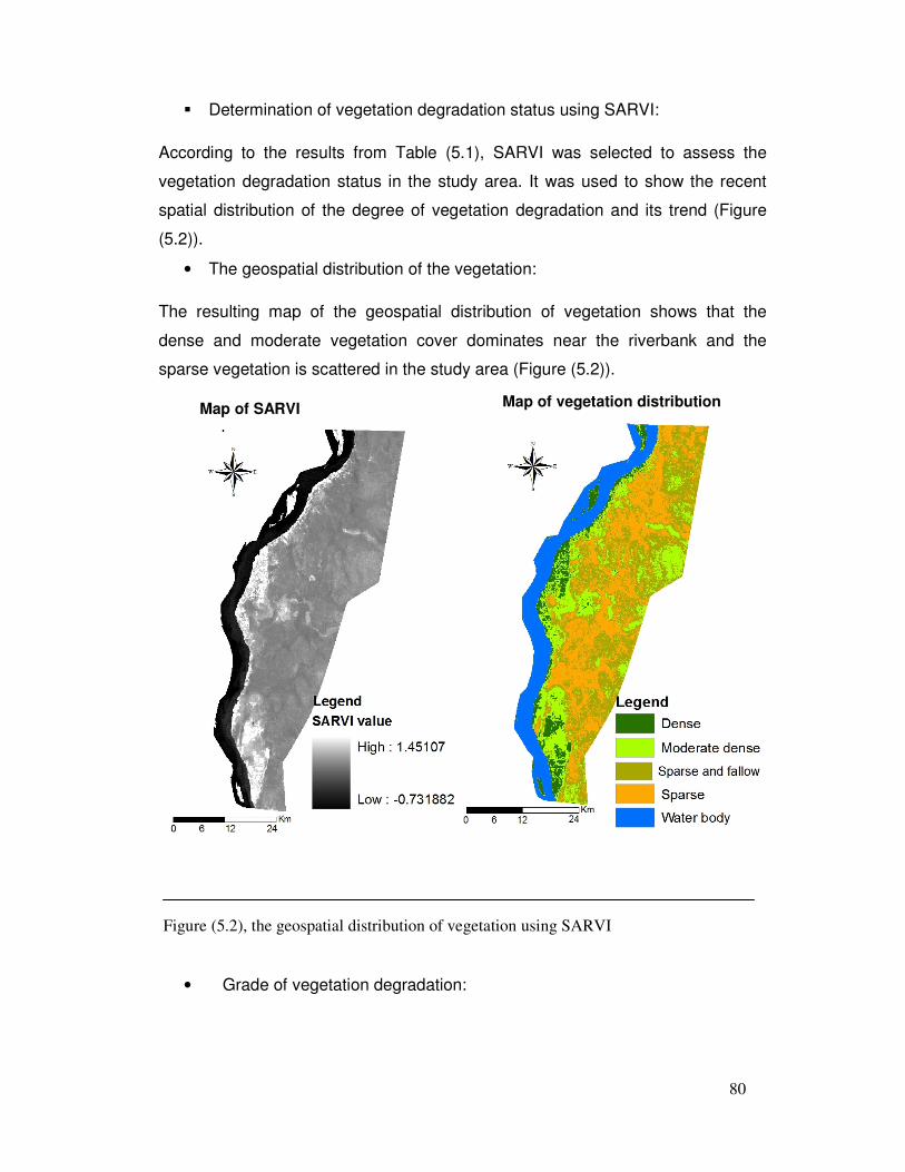
80
� Determination of vegetation degradation status using SARVI:
According to the results from Table (5.1), SARVI was selected to assess the
vegetation degradation status in the study area. It was used to show the recent
spatial distribution of the degree of vegetation degradation and its trend (Figure
(5.2)).
• The geospatial distribution of the vegetation:
The resulting map of the geospatial distribution of vegetation shows that the
dense and moderate vegetation cover dominates near the riverbank and the
sparse vegetation is scattered in the study area (Figure (5.2)).
Figure (5.2), the geospatial distribution of vegetation using SARVI
• Grade of vegetation degradation:
Map of SARVI Map of vegetation distribution
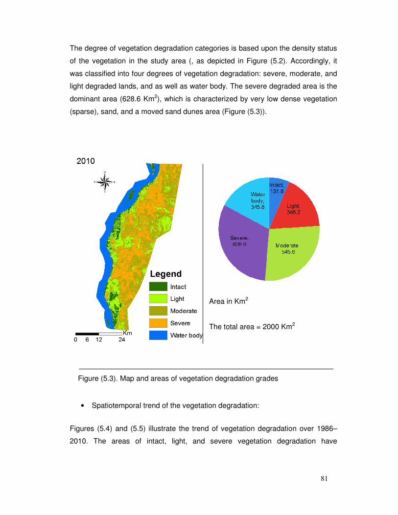
81
The degree of vegetation degradation categories is based upon the density status
of the vegetation in the study area (, as depicted in Figure (5.2). Accordingly, it
was classified into four degrees of vegetation degradation: severe, moderate, and
light degraded lands, and as well as water body. The severe degraded area is the
dominant area (628.6 Km2), which is characterized by very low dense vegetation
(sparse), sand, and a moved sand dunes area (Figure (5.3)).
Area in Km2
The total area = 2000 Km2
Figure (5.3). Map and areas of vegetation degradation grades
• Spatiotemporal trend of the vegetation degradation:
Figures (5.4) and (5.5) illustrate the trend of vegetation degradation over 1986–
2010. The areas of intact, light, and severe vegetation degradation have
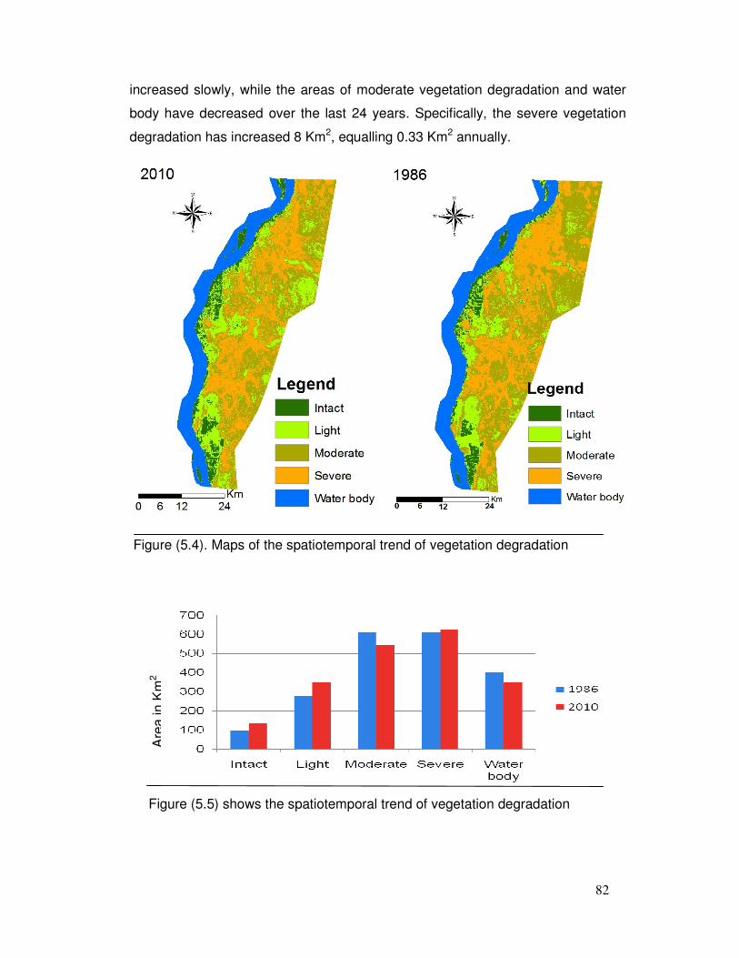
82
increased slowly, while the areas of moderate vegetation degradation and water
body have decreased over the last 24 years. Specifically, the severe vegetation
degradation has increased 8 Km2, equalling 0.33 Km2 annually.
Figure (5.4). Maps of the spatiotemporal trend of vegetation degradation
Figure (5.5) shows the spatiotemporal trend of vegetation degradation
Are
a in
Km
2
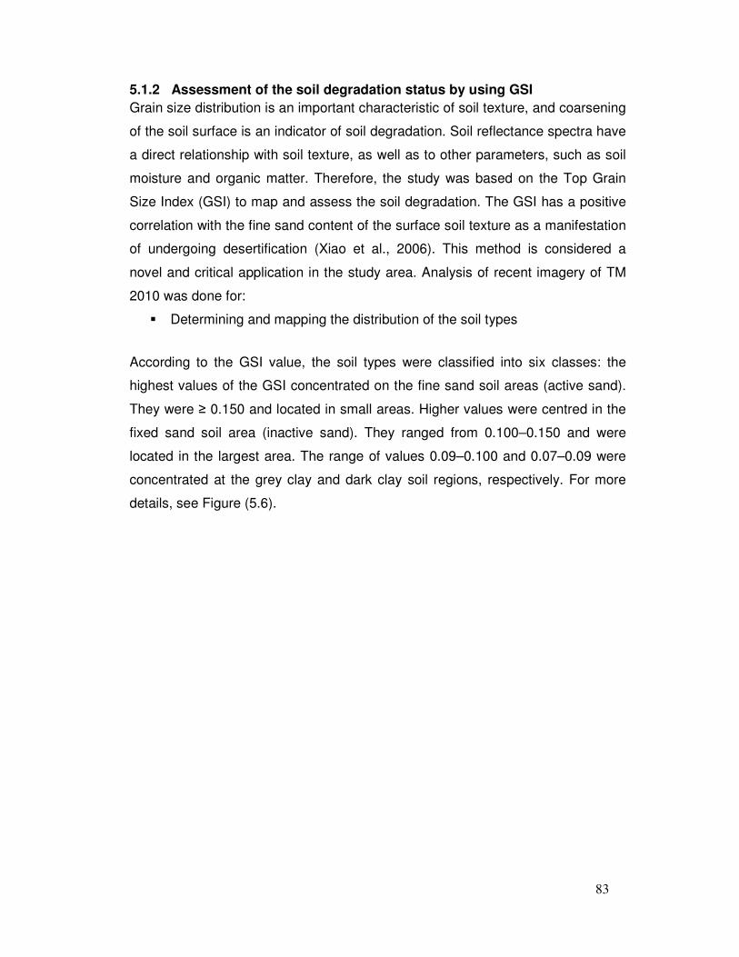
83
5.1.2 Assessment of the soil degradation status by using GSI
Grain size distribution is an important characteristic of soil texture, and coarsening
of the soil surface is an indicator of soil degradation. Soil reflectance spectra have
a direct relationship with soil texture, as well as to other parameters, such as soil
moisture and organic matter. Therefore, the study was based on the Top Grain
Size Index (GSI) to map and assess the soil degradation. The GSI has a positive
correlation with the fine sand content of the surface soil texture as a manifestation
of undergoing desertification (Xiao et al., 2006). This method is considered a
novel and critical application in the study area. Analysis of recent imagery of TM
2010 was done for:
� Determining and mapping the distribution of the soil types
According to the GSI value, the soil types were classified into six classes: the
highest values of the GSI concentrated on the fine sand soil areas (active sand).
They were ≥ 0.150 and located in small areas. Higher values were centred in the
fixed sand soil area (inactive sand). They ranged from 0.100–0.150 and were
located in the largest area. The range of values 0.09–0.100 and 0.07–0.09 were
concentrated at the grey clay and dark clay soil regions, respectively. For more
details, see Figure (5.6).
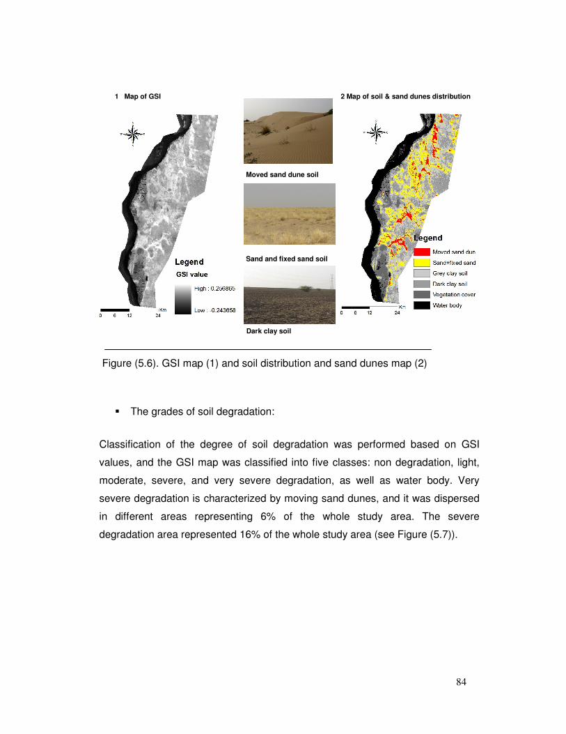
84
1 Map of GSI 2 Map of soil & sand dunes distribution
Moved sand dune soil
Sand and fixed sand soil
Dark clay soil
Figure (5.6). GSI map (1) and soil distribution and sand dunes map (2)
� The grades of soil degradation:
Classification of the degree of soil degradation was performed based on GSI
values, and the GSI map was classified into five classes: non degradation, light,
moderate, severe, and very severe degradation, as well as water body. Very
severe degradation is characterized by moving sand dunes, and it was dispersed
in different areas representing 6% of the whole study area. The severe
degradation area represented 16% of the whole study area (see Figure (5.7)).
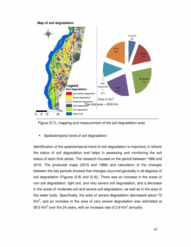
85
Map of soil degradation
Area in Km2
The total area = 2000 Km
Figure (5.7), mapping and measurement of the soil degradation area
� Spatiotemporal trend of soil degradation:
Identification of the spatiotemporal trend of soil degradation is important; it reflects
the status of soil degradation and helps in assessing and monitoring the soil
status of each time series. The research focused on the period between 1986 and
2010. The produced maps (2010 and 1986) and calculation of the changes
between the two periods showed that changes occurred generally in all degrees of
soil degradation (Figures (5.8) and (5.9)). There was an increase in the areas of
non soil degradation, light soil, and very severe soil degradation, and a decrease
in the areas of moderate soil and severe soil degradation, as well as in the area of
the water body. Specifically, the area of severe degradation decreased about 73
Km2, and an increase in the area of very severe degradation was estimated at
69.5 Km2 over the 24 years, with an increase rate of 2.9 Km2 annually.
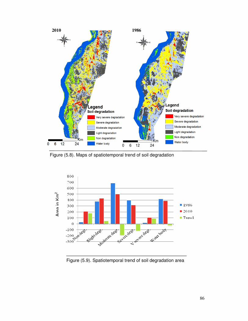
86
Km0 12 246
Figure (5.8). Maps of spatiotemporal trend of soil degradation
Figure (5.9). Spatiotemporal trend of soil degradation area
Are
a in
Km
2
2010 1986
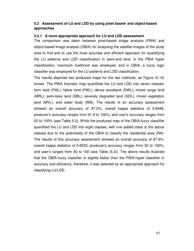
87
5.2 Assessment of LU and LDD by using pixel based- and object-based
approaches
5.2.1 A more appropriate approach for LU and LDD assessment
The comparison was taken between pixel-based image analysis (PBIA) and
object-based image analysis (OBIA) for analysing the satellite images of the study
area to find and to use the most accurate and efficient approach for quantifying
the LU patterns and LDD classification in semi-arid land. In the PBIA hyper
classification, maximum livelihood was employed, and in OBIA, a fuzzy logic
classifier was employed for the LU patterns and LDD classification.
The results depicted two produced maps for the two methods, as Figure (5.10)
shows. The PBIA thematic map quantified the LU and LDD into seven classes:
farm land (FML); fallow land (FWL); dense woodland (DWL); mixed range land
(MRL); semi-bare land (SBL); severely degraded land (SDL); mixed vegetation
land (MVL); and water body (WB). The results of an accuracy assessment
showed an overall accuracy of 87.2%; overall kappa statistics of 0.8448;
producer’s accuracy ranges from 61.9 to 100%; and user’s accuracy ranges from
52 to 100% (see Table 5.2). While the produced map of the OBIA-fuzzy classifier
quantified the LU and LDD into eight classes, with one added class to the above
classes due to the potentiality of the OBIA to classify the residential area (RA).
The results of this accuracy assessment showed an overall accuracy of 87.6%;
overall kappa statistics of 0.8522; producer’s accuracy ranges from 52 to 100%;
and user’s ranges from 50 to 100 (see Table (5.3)). The above results illustrate
that the OBIA-fuzzy classifier is slightly better than the PBIA-hyper classifier in
accuracy and efficiency; therefore, it was selected as an appropriate approach for
classifying LU/LDD.
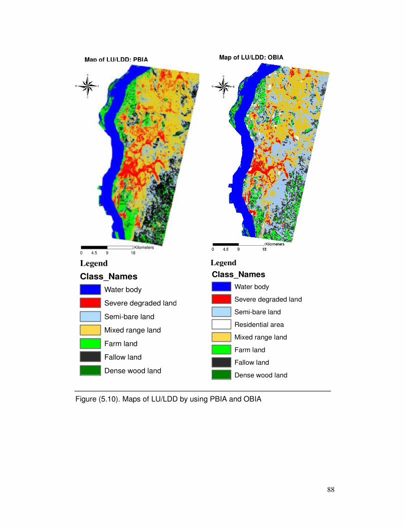
88
Map of LU/LDD: PBIA Map of LU/LDD: OBIA
Legend
Class_Names
Water body
Severe degraded land
Semi-bare land
Residential area
Mixed range land
Farm land
Fallow land
Dense wood land
Legend
Class_Names
Water body
Severe degraded land
Semi-bare land
Mixed range land
Farm land
Fallow land
Dense wood land
Figure (5.10). Maps of LU/LDD by using PBIA and OBIA
®
0 9 184.5Kilometers
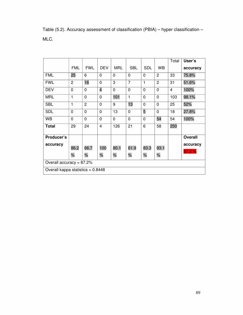
89
Table (5.2). Accuracy assessment of classification (PBIA) – hyper classification –
MLC.
FML
FWL
DEV
MRL
SBL
SDL
WB
Total User’s
accuracy
FML 25 6 0 0 0 0 2 33 75.8%
FWL 2 16 0 3 7 1 2 31 51.6%
DEV 0 0 4 0 0 0 0 4 100%
MRL 1 0 0 101 1 0 0 103 98.1%
SBL 1 2 0 9 13 0 0 25 52%
SDL 0 0 0 13 0 5 0 18 27.8%
WB 0 0 0 0 0 0 54 54 100%
Total 29 24 4 126 21 6 58 250
Producer’s
accuracy
86.2
%
66.7
%
100
%
80.1
%
61.9
%
83.3
%
93.1
%
Overall
accuracy
87.2 %
Overall accuracy = 87.2%
Overall kappa statistics = 0.8448
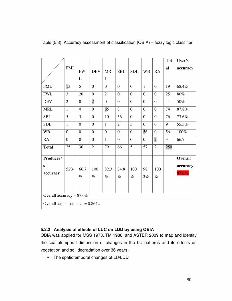
90
Table (5.3). Accuracy assessment of classification (OBIA) – fuzzy logic classifier
5.2.2 Analysis of effects of LUC on LDD by using OBIA
OBIA was applied for MSS 1973, TM 1986, and ASTER 2009 to map and identify
the spatiotemporal dimension of changes in the LU patterns and its effects on
vegetation and soil degradation over 36 years:
� The spatiotemporal changes of LU/LDD
FML
FW
L
DEV
MR
L
SBL
SDL
WB
RA
Tot
al
User’s
accuracy
FML 13 5 0 0 0 0 1 0 19 68.4%
FWL 3 20 0 2 0 0 0 0 25 80%
DEV 2 0 2 0 0 0 0 0 4 50%
MRL 1 0 0 65 8 0 0 0 74 87.8%
SBL 5 5 0 10 56 0 0 0 76 73.6%
SDL 1 0 0 1 2 5 0 0 9 55.5%
WB 0 0 0 0 0 0 56 0 56 100%
RA 0 0 0 1 0 0 0 2 3 66.7
Total 25 30 2 79 66 5 57 2 250
Producer’
s
accuracy
52%
66.7
%
100
%
82.3
%
84.8
%
100
%
98.
2%
100
%
Overall
accuracy
87.6%
Overall accuracy = 87.6%
Overall kappa statistics = 0.8642
91
Three thematic maps of the LU/LDD were produced by OBIA: the LU/LDD from
1973, 1986, and 2009. Obviously, the three maps reflect the changes that
occurred to the LU/LDD classes from 1973–1986 and 1986–2009 (Figure (5.11)).
Table (5.4) shows the areas of the different classes of the LU/LDD that cover the
study area for the three periods and the changing areas. The important results
show that in 1973, the area of MRL was the biggest area, estimated as 636 Km2,
representing 39.8% of the total area, while the residential area (RA) was the small
one, estimated at 9.6 Km2. Moreover, the area of severe degraded land (SDL) was
88.1 Km2, representing 5.5% of the total area.
In 1986, the semi bare land (SBL) was the largest one, estimated at 509 Km2,
representing 31.8%. The area of SDL decreased to 81.8 Km2, equalising 5.1% of
the total study area. In 2009, the SBL was still the largest and the RA was the
smallest. Figure (5.12) shows that changes took place in the all LU/ LDD
categories in both periods of 1973–1986 and 1986–2009. In 1973–1986, the
results show that an increased change trend occurred remarkably in the areas of
dense woodland (DWL), RA, SBL and fallow land (FWL), as well as in the water
body (WB).
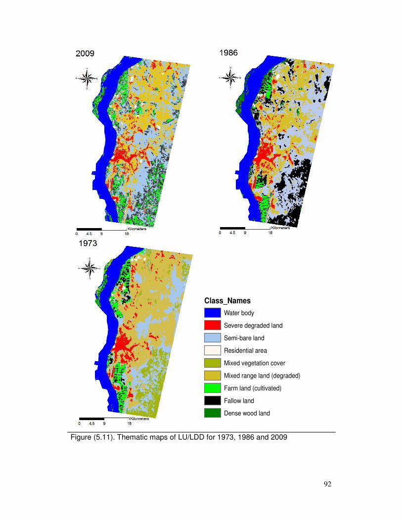
92
Figure (5.11). Thematic maps of LU/LDD for 1973, 1986 and 2009
Class_Names
Water body
Severe degraded land
Semi-bare land
Residential area
Mixed vegetation cover
Mixed range land (degraded)
Farm land (cultivated)
Fallow land
Dense wood land
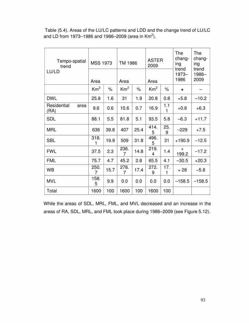
93
Table (5.4). Areas of the LU/LC patterns and LDD and the change trend of LU/LC and LD from 1973–1986 and 1986–2009 (area in Km2).
While the areas of SDL, MRL, FML, and MVL decreased and an increase in the
areas of RA, SDL, MRL, and FML took place during 1986–2009 (see Figure 5.12).
Tempo-spatial trend
LU/LD
MSS 1973
TM 1986
ASTER 2009
The chang-ing trend 1973–1986
The chang-ing trend 1986–2009
Area
Area
Area
Km2 % Km2 % Km2 % + –
DWL 25.8 1.6 31 1.9 20.8 0.8 +5.8 –10.2
Residential area (RA) 9.6 0.6 10.6 0.7 16.9 1.1
1 +0.8 +6.3
SDL 88.1 5.5 81.8 5.1 93.5 5.8 –6.3 +11.7
MRL 636 39.8 407 25.4 414.5
25.9 –229 +7.5
SBL 318.1 19.9 509 31.8 496.
5 31 +190.9 –12.5
FWL 37.5 2.3 236.
7 14.8 219.
4 1.4 +
199.2 –17.2
FML 75.7 4.7 45.2 2.8 65.5 4.1 –30.5 +20.3
WB 250.7 15.7 278.
7 17.4 272.9
17.1 + 28 –5.8
MVL 158.5 9.9 0.0 0.0 0.0 0.0 –158.5 –158.5
Total 1600 100 1600 100 1600 100
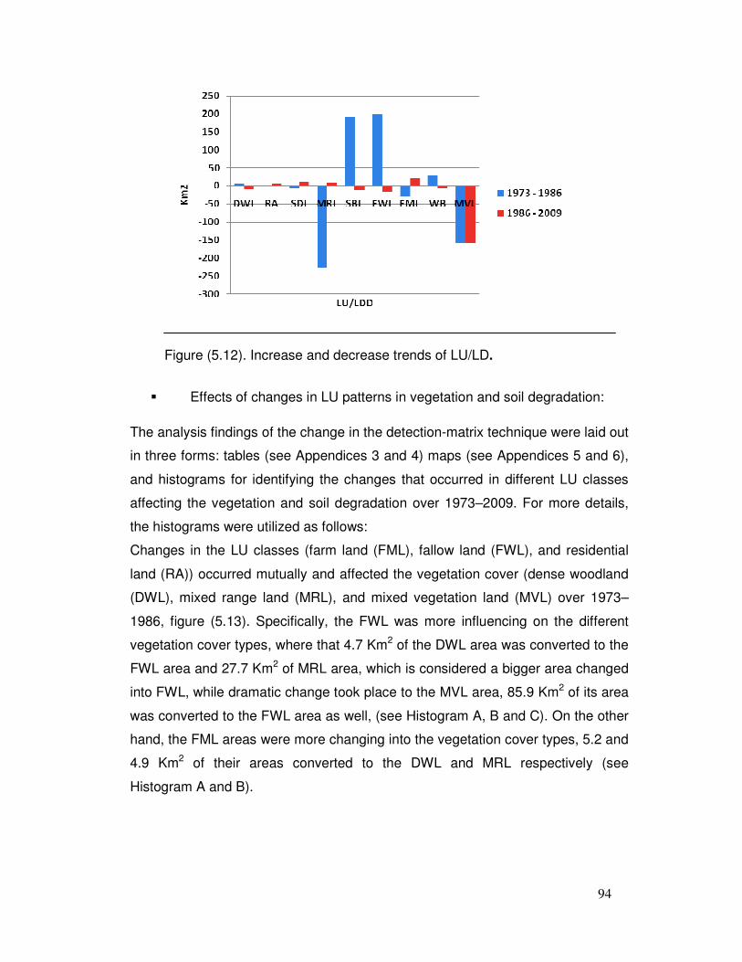
94
Figure (5.12). Increase and decrease trends of LU/LD.
� Effects of changes in LU patterns in vegetation and soil degradation:
The analysis findings of the change in the detection-matrix technique were laid out
in three forms: tables (see Appendices 3 and 4) maps (see Appendices 5 and 6),
and histograms for identifying the changes that occurred in different LU classes
affecting the vegetation and soil degradation over 1973–2009. For more details,
the histograms were utilized as follows:
Changes in the LU classes (farm land (FML), fallow land (FWL), and residential
land (RA)) occurred mutually and affected the vegetation cover (dense woodland
(DWL), mixed range land (MRL), and mixed vegetation land (MVL) over 1973–
1986, figure (5.13). Specifically, the FWL was more influencing on the different
vegetation cover types, where that 4.7 Km2 of the DWL area was converted to the
FWL area and 27.7 Km2 of MRL area, which is considered a bigger area changed
into FWL, while dramatic change took place to the MVL area, 85.9 Km2 of its area
was converted to the FWL area as well, (see Histogram A, B and C). On the other
hand, the FML areas were more changing into the vegetation cover types, 5.2 and
4.9 Km2 of their areas converted to the DWL and MRL respectively (see
Histogram A and B).
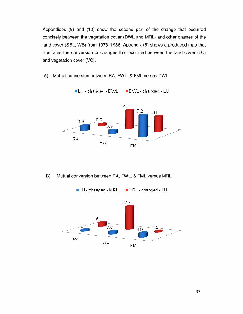
95
Appendices (9) and (10) show the second part of the change that occurred
concisely between the vegetation cover (DWL and MRL) and other classes of the
land cover (SBL, WB) from 1973–1986. Appendix (5) shows a produced map that
illustrates the conversion or changes that occurred between the land cover (LC)
and vegetation cover (VC).
A) Mutual conversion between RA, FWL, & FML versus DWL
B) Mutual conversion between RA, FWL, & FML versus MRL
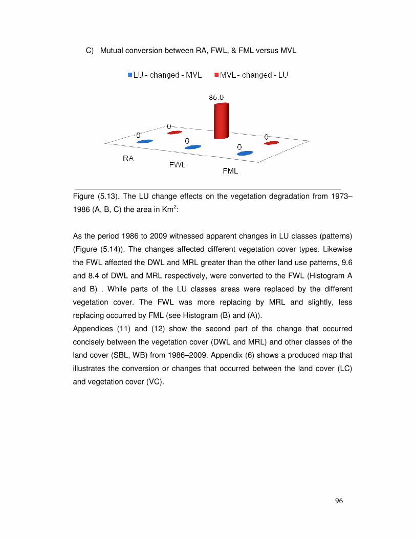
96
C) Mutual conversion between RA, FWL, & FML versus MVL
Figure (5.13). The LU change effects on the vegetation degradation from 1973–
1986 (A, B, C) the area in Km2:
As the period 1986 to 2009 witnessed apparent changes in LU classes (patterns)
(Figure (5.14)). The changes affected different vegetation cover types. Likewise
the FWL affected the DWL and MRL greater than the other land use patterns, 9.6
and 8.4 of DWL and MRL respectively, were converted to the FWL (Histogram A
and B) . While parts of the LU classes areas were replaced by the different
vegetation cover. The FWL was more replacing by MRL and slightly, less
replacing occurred by FML (see Histogram (B) and (A)).
Appendices (11) and (12) show the second part of the change that occurred
concisely between the vegetation cover (DWL and MRL) and other classes of the
land cover (SBL, WB) from 1986–2009. Appendix (6) shows a produced map that
illustrates the conversion or changes that occurred between the land cover (LC)
and vegetation cover (VC).
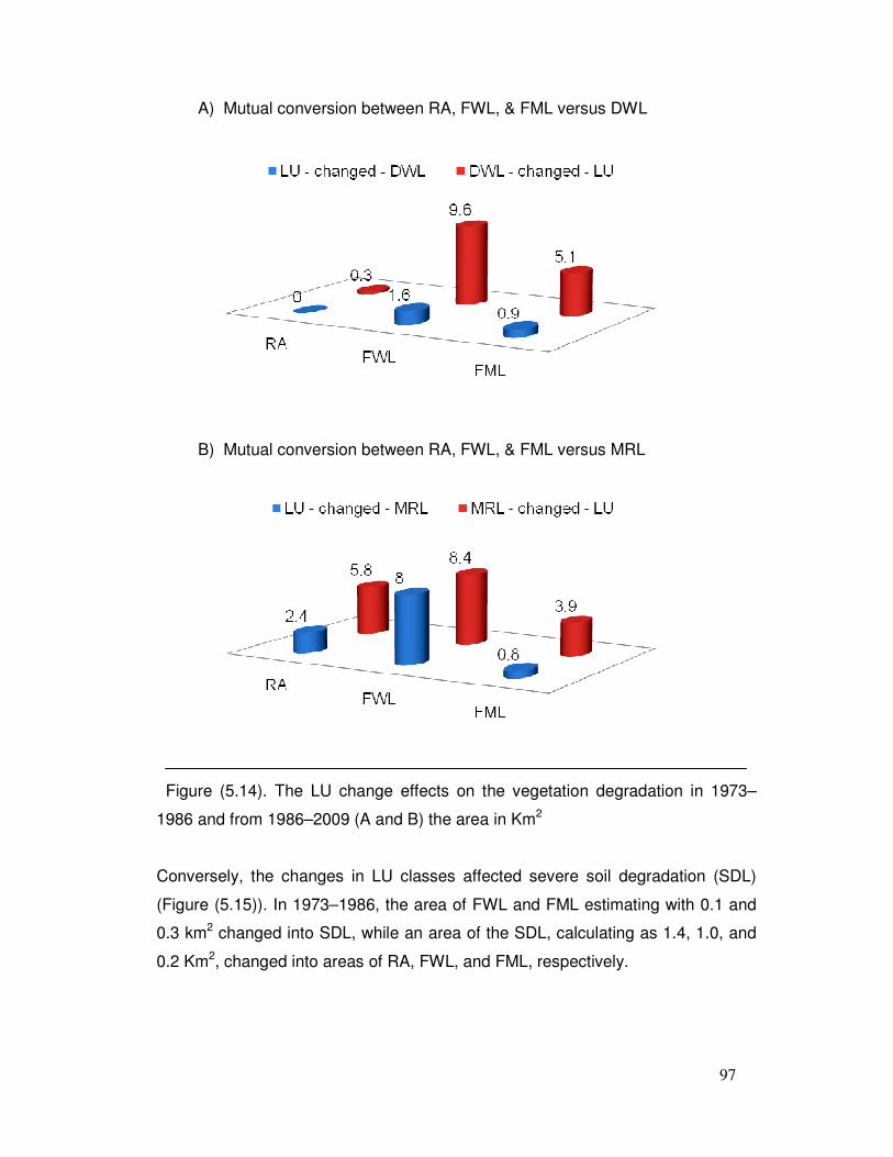
97
A) Mutual conversion between RA, FWL, & FML versus DWL
B) Mutual conversion between RA, FWL, & FML versus MRL
Figure (5.14). The LU change effects on the vegetation degradation in 1973–
1986 and from 1986–2009 (A and B) the area in Km2
Conversely, the changes in LU classes affected severe soil degradation (SDL)
(Figure (5.15)). In 1973–1986, the area of FWL and FML estimating with 0.1 and
0.3 km2 changed into SDL, while an area of the SDL, calculating as 1.4, 1.0, and
0.2 Km2, changed into areas of RA, FWL, and FML, respectively.
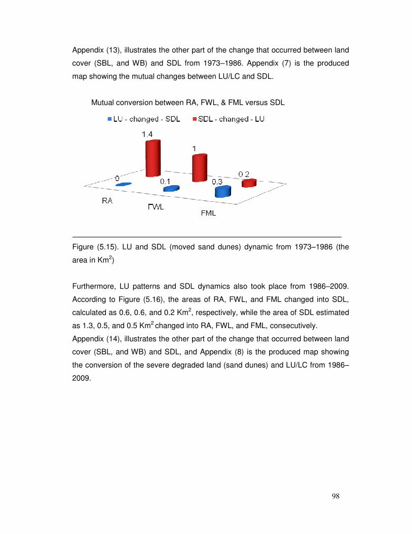
98
Appendix (13), illustrates the other part of the change that occurred between land
cover (SBL, and WB) and SDL from 1973–1986. Appendix (7) is the produced
map showing the mutual changes between LU/LC and SDL.
Mutual conversion between RA, FWL, & FML versus SDL
Figure (5.15). LU and SDL (moved sand dunes) dynamic from 1973–1986 (the
area in Km2)
Furthermore, LU patterns and SDL dynamics also took place from 1986–2009.
According to Figure (5.16), the areas of RA, FWL, and FML changed into SDL,
calculated as 0.6, 0.6, and 0.2 Km2, respectively, while the area of SDL estimated
as 1.3, 0.5, and 0.5 Km2 changed into RA, FWL, and FML, consecutively.
Appendix (14), illustrates the other part of the change that occurred between land
cover (SBL, and WB) and SDL, and Appendix (8) is the produced map showing
the conversion of the severe degraded land (sand dunes) and LU/LC from 1986–
2009.
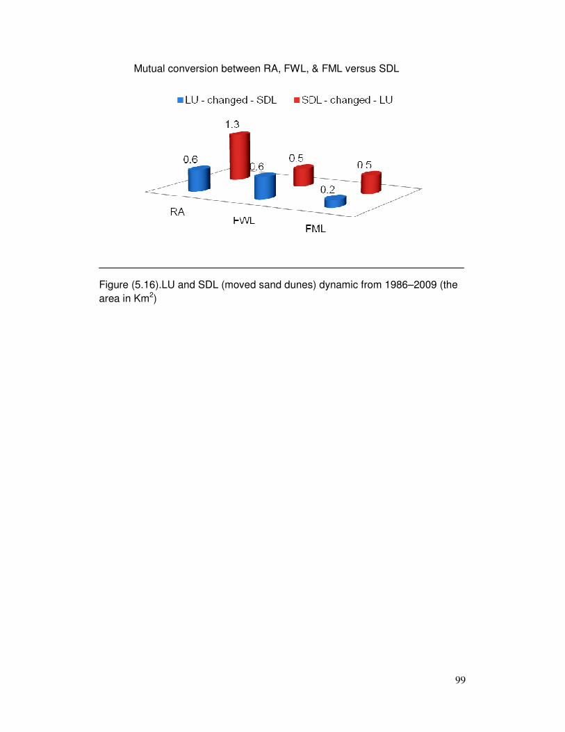
99
Mutual conversion between RA, FWL, & FML versus SDL
Figure (5.16).LU and SDL (moved sand dunes) dynamic from 1986–2009 (the area in Km2)
100
5.3 Modelling the influence of LUC on LDD
The study aimed at modelling the impacts of LU patterns on LD based on soil
degradation (sand dunes) and vegetation degradation for identifying the
relationship between LD (as dependent variable) and different patterns of LU (as
independent variable), and moreover it attempted to predict the effects of LUC on
LD in the semi-arid zone (study area). Multiple linear regression models were
used for building two LD models: soil degradation and vegetation degradation
influenced by LU patterns. Appendix (15) is a table of the time series of the
remote sensing data set of the LU and LD classes. This is in addition to the time
series of climatic and population growth data, during 1973–2009, which was used
in a Pearson correlation matrix and multiple linear regression analysis.
5.3.1 Model building of LU patterns affecting LDD
Modelling the LU patterns affecting vegetation cover degradation (VCD)
Modelling the LU patterns affecting soil degradation land (SDL) based on sand
dunes
LUC, VCD, and SDL information were obtained from the results of the RS and
GIS analysis. The resulting classes of LU/LC are vegetation cover (dense
vegetation land (DWL) + mixed range land (MRL)), farm land (FML), fallow land
(FWL) and residential area (RA) (see Table (5.5) and Appendix (15)). Different
processes were done for above data to build the required model:
Correlation coefficient matrix:-
The regression analysis commenced by first estimating the correlation coefficient
matrix for all variables to obtain an approximate solution for an idea of the
relationships between predictors and outcome and for a preliminary look for
multicollinearity. The resultant table (Table 5.5) shows very strong correlations (R
> 0.9). However, these very strong correlations are not among the independent
variables; therefore, no multicollinearaty violation could be expected during the
regression analysis for establishing the desirable models.
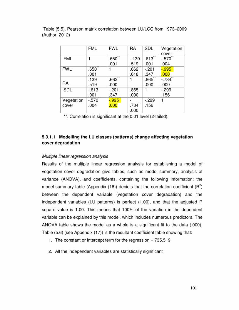
101
Table (5.5). Pearson matrix correlation between LU/LCC from 1973–2009 (Author, 2012)
FML FWL RA SDL Vegetation cover
FML 1 .650** .001
-.139 .519
.613**
.001 -.570** .004
FWL .650** .001
1 .662** .618
-.201 .347
-.995** .000
RA .139 .519
.662**
.000 1 .865**
.000 -.734**
.000 SDL -.613
.001 -.201 .347
.865
.000 1 -.299
.156 Vegetation cover
-.570** .004
-.995** .000
-.734** .000
-.299 .156
1
**. Correlation is significant at the 0.01 level (2-tailed).
5.3.1.1 Modelling the LU classes (patterns) change affecting vegetation
cover degradation
Multiple linear regression analysis
Results of the multiple linear regression analysis for establishing a model of
vegetation cover degradation give tables, such as model summary, analysis of
variance (ANOVA), and coefficients, containing the following information: the
model summary table (Appendix (16)) depicts that the correlation coefficient (R2)
between the dependent variable (vegetation cover degradation) and the
independent variables (LU patterns) is perfect (1.00), and that the adjusted R
square value is 1.00. This means that 100% of the variation in the dependent
variable can be explained by this model, which includes numerous predictors. The
ANOVA table shows the model as a whole is a significant fit to the data (.000).
Table (5.6) (see Appendix (17)) is the resultant coefficient table showing that:
1. The constant or intercept term for the regression = 735.519
2. All the independent variables are statistically significant
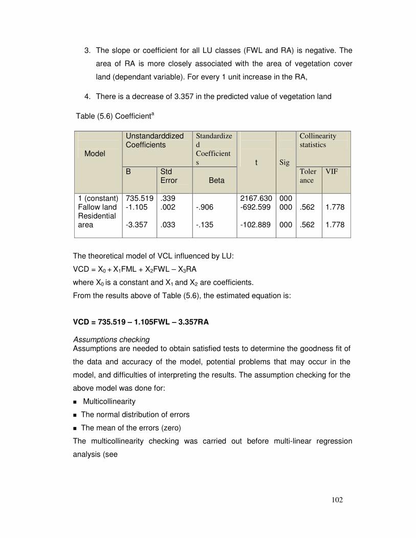
102
3. The slope or coefficient for all LU classes (FWL and RA) is negative. The
area of RA is more closely associated with the area of vegetation cover
land (dependant variable). For every 1 unit increase in the RA,
4. There is a decrease of 3.357 in the predicted value of vegetation land
Table (5.6) Coefficienta
Model
Unstandarddized Coefficients
Standardize
d
Coefficient
s
t
Sig
Collinearity
statistics
B
Std Error
Beta Toler
ance
VIF
1 (constant) Fallow land Residential area
735.519 -1.105 -3.357
.339
.002 .033
-.906 -.135
2167.630 -692.599 -102.889
000 000 000
.562 .562
1.778 1.778
The theoretical model of VCL influenced by LU:
VCD = X0 + X1FML + X2FWL – X3RA
where X0 is a constant and X1 and X2 are coefficients.
From the results above of Table (5.6), the estimated equation is: VCD = 735.519 – 1.105FWL – 3.357RA Assumptions checking Assumptions are needed to obtain satisfied tests to determine the goodness fit of
the data and accuracy of the model, potential problems that may occur in the
model, and difficulties of interpreting the results. The assumption checking for the
above model was done for:
� Multicollinearity
� The normal distribution of errors
� The mean of the errors (zero)
The multicollinearity checking was carried out before multi-linear regression
analysis (see
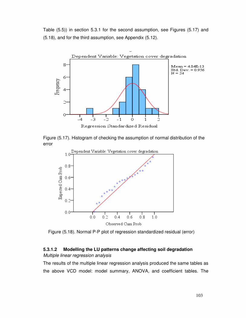
103
Table (5.5)) in section 5.3.1 for the second assumption, see Figures (5.17) and
(5.18), and for the third assumption, see Appendix (5.12).
Figure (5.17). Histogram of checking the assumption of normal distribution of the error
Figure (5.18). Normal P-P plot of regression standardized residual (error)
5.3.1.2 Modelling the LU patterns change affecting soil degradation
Multiple linear regression analysis
The results of the multiple linear regression analysis produced the same tables as
the above VCD model: model summary, ANOVA, and coefficient tables. The
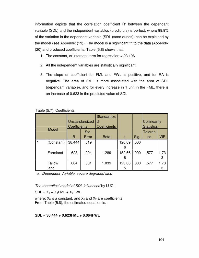
104
information depicts that the correlation coefficient R2 between the dependant
variable (SDL) and the independent variables (predictors) is perfect, where 99.9%
of the variation in the dependent variable (SDL (sand dunes)) can be explained by
the model (see Appendix (19)). The model is a significant fit to the data (Appendix
(20) and produced coefficients. Table (5.8) shows that:
1. The constant, or intercept term for regression = 23.196
2. All the independent variables are statistically significant
3. The slope or coefficient for FML and FWL is positive, and for RA is
negative. The area of FML is more associated with the area of SDL
(dependant variable), and for every increase in 1 unit in the FML, there is
an increase of 0.623 in the predicted value of SDL
Table (5.7). Coefficients
Model
Unstandardized Coefficients
Standardized Coefficients
t Sig.
Collinearity Statistics
B Std. Error Beta
Tolerance VIF
1 (Constant) 38.444 .319 120.696
.000
Farmland .623 .004 1.289 152.668
.000 .577 1.733
Fallow land
.064 .001 1.039 123.065
.000 .577 1.733
a. Dependent Variable: severe degraded land
The theoretical model of SDL influenced by LUC:
SDL = X0 + X1FML + X2FWL
where: X0 is a constant, and X1 and X2 are coefficients. From Table (5.8), the estimated equation is:
SDL = 38.444 + 0.623FML + 0.064FWL
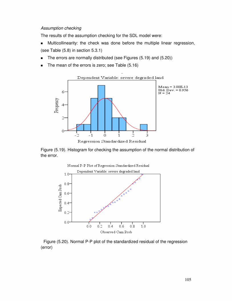
105
Assumption checking
The results of the assumption checking for the SDL model were:
� Multicollinearity: the check was done before the multiple linear regression,
(see Table (5.8) in section 5.3.1)
� The errors are normally distributed (see Figures (5.19) and (5.20))
� The mean of the errors is zero; see Table (5.16)
Figure (5.19). Histogram for checking the assumption of the normal distribution of the error.
Figure (5.20). Normal P-P plot of the standardized residual of the regression (error)
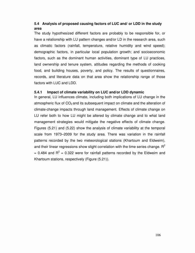
106
5.4 Analysis of proposed causing factors of LUC and/ or LDD in the study
area
The study hypothesized different factors are probably to be responsible for, or
have a relationship with LU pattern changes and/or LD in the research area, such
as climatic factors (rainfall, temperature, relative humidity and wind speed);
demographic factors, in particular local population growth; and socioeconomic
factors, such as the dominant human activities, dominant type of LU practices,
land ownership and tenure system, attitudes regarding the methods of cooking
food, and building houses, poverty, and policy. The results of questionnaires,
records, and literature data on that area show the relationship range of those
factors with LUC and LDD.
5.4.1 Impact of climate variability on LUC and/or LDD dynamic
In general, LU influences climate, including both implications of LU change in the
atmospheric flux of CO2 and its subsequent impact on climate and the alteration of
climate-change impacts through land management. Effects of climate change on
LU refer both to how LU might be altered by climate change and to what land
management strategies would mitigate the negative effects of climate change.
Figures (5.21) and (5.22) show the analysis of climate variability at the temporal
scale from 1973–2009 for the study area. There was variation in the rainfall
patterns recorded by the two meteorological stations (Khartoum and Eldweim),
and their linear regressions show slight correlation with the time series change. R2
= 0.484 and R2 = 0.322 were for rainfall patterns recorded by the Eldweim and
Khartoum stations, respectively (Figure (5.21)).
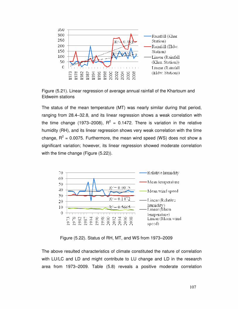
107
Figure (5.21). Linear regression of average annual rainfall of the Khartoum and Eldweim stations
The status of the mean temperature (MT) was nearly similar during that period,
ranging from 28.4–32.8, and its linear regression shows a weak correlation with
the time change (1973–2008), R2 = 0.1472. There is variation in the relative
humidity (RH), and its linear regression shows very weak correlation with the time
change, R2 = 0.0075. Furthermore, the mean wind speed (WS) does not show a
significant variation; however, its linear regression showed moderate correlation
with the time change (Figure (5.22)).
Figure (5.22). Status of RH, MT, and WS from 1973–2009
The above resulted characteristics of climate constituted the nature of correlation
with LU/LC and LD and might contribute to LU change and LD in the research
area from 1973–2009. Table (5.8) reveals a positive moderate correlation
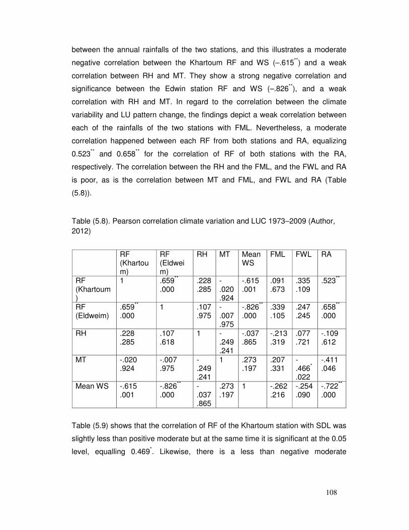
108
between the annual rainfalls of the two stations, and this illustrates a moderate
negative correlation between the Khartoum RF and WS (–.615**) and a weak
correlation between RH and MT. They show a strong negative correlation and
significance between the Edwin station RF and WS (–.826**), and a weak
correlation with RH and MT. In regard to the correlation between the climate
variability and LU pattern change, the findings depict a weak correlation between
each of the rainfalls of the two stations with FML. Nevertheless, a moderate
correlation happened between each RF from both stations and RA, equalizing
0.523** and 0.658** for the correlation of RF of both stations with the RA,
respectively. The correlation between the RH and the FML, and the FWL and RA
is poor, as is the correlation between MT and FML, and FWL and RA (Table
(5.8)).
Table (5.8). Pearson correlation climate variation and LUC 1973–2009 (Author, 2012)
RF (Khartoum)
RF (Eldweim)
RH MT Mean WS
FML FWL RA
RF (Khartoum)
1 .659** .000
.228
.285 -.020 .924
-.615 .001
.091
.673 .335 .109
.523**
RF (Eldweim)
.659**
.000 1 .107
.975 -.007 .975
-.826** .000
.339
.105 .247 .245
.658**
.000
RH .228 .285
.107
.618 1 -
.249
.241
-.037 .865
-.213 .319
.077
.721 -.109 .612
MT -.020 .924
-.007 .975
-.249 .241
1 .273 .197
.207
.331 -.466*
.022
-.411 .046
Mean WS -.615 .001
-.826** .000
-.037 .865
.273
.197 1 -.262
.216 -.254 .090
-.722** .000
Table (5.9) shows that the correlation of RF of the Khartoum station with SDL was
slightly less than positive moderate but at the same time it is significant at the 0.05
level, equalling 0.469*. Likewise, there is a less than negative moderate
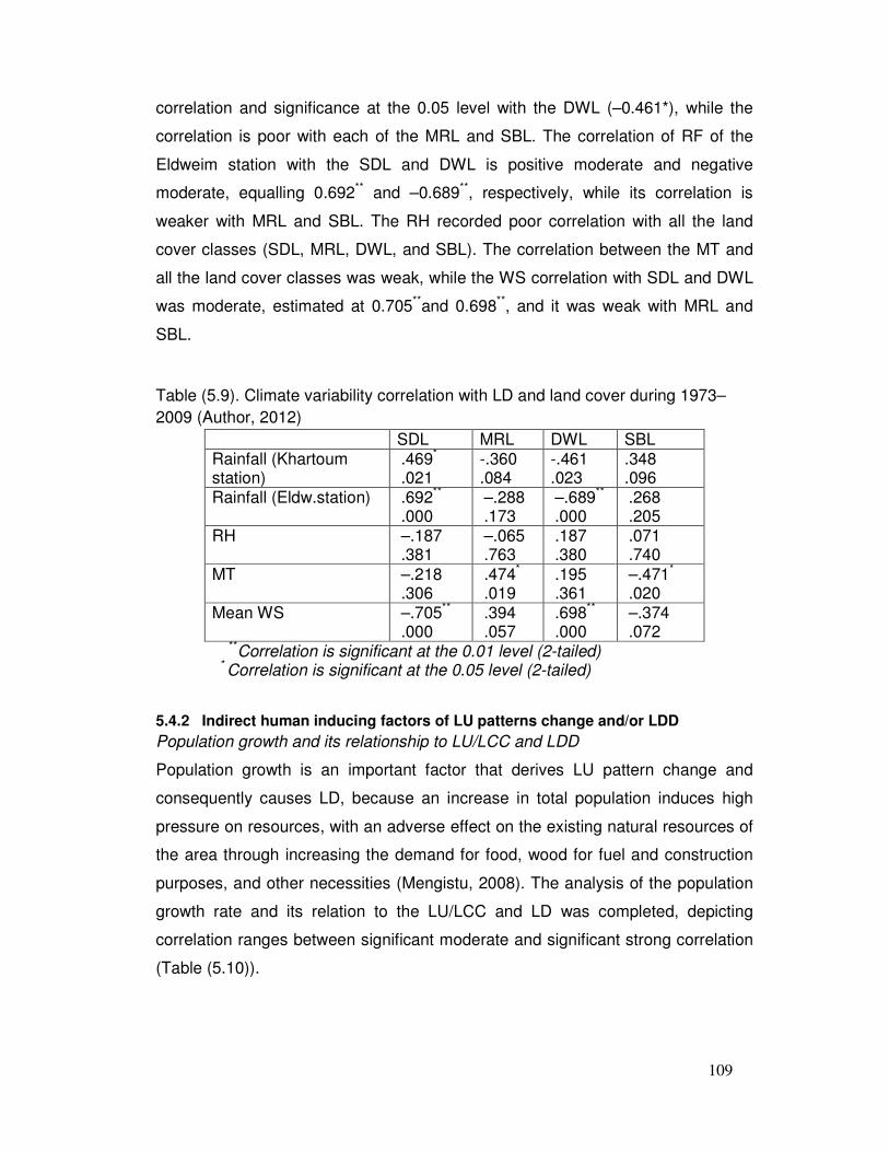
109
correlation and significance at the 0.05 level with the DWL (–0.461*), while the
correlation is poor with each of the MRL and SBL. The correlation of RF of the
Eldweim station with the SDL and DWL is positive moderate and negative
moderate, equalling 0.692** and –0.689**, respectively, while its correlation is
weaker with MRL and SBL. The RH recorded poor correlation with all the land
cover classes (SDL, MRL, DWL, and SBL). The correlation between the MT and
all the land cover classes was weak, while the WS correlation with SDL and DWL
was moderate, estimated at 0.705**and 0.698**, and it was weak with MRL and
SBL.
Table (5.9). Climate variability correlation with LD and land cover during 1973–2009 (Author, 2012)
SDL MRL DWL SBL Rainfall (Khartoum station)
.469*
.021 -.360 .084
-.461 .023
.348
.096 Rainfall (Eldw.station) .692**
.000 –.288 .173
–.689** .000
.268
.205 RH –.187
.381 –.065 .763
.187
.380 .071 .740
MT –.218 .306
.474*
.019 .195 .361
–.471* .020
Mean WS –.705** .000
.394
.057 .698** .000
–.374 .072
**Correlation is significant at the 0.01 level (2-tailed) * Correlation is significant at the 0.05 level (2-tailed)
5.4.2 Indirect human inducing factors of LU patterns change and/or LDD
Population growth and its relationship to LU/LCC and LDD
Population growth is an important factor that derives LU pattern change and
consequently causes LD, because an increase in total population induces high
pressure on resources, with an adverse effect on the existing natural resources of
the area through increasing the demand for food, wood for fuel and construction
purposes, and other necessities (Mengistu, 2008). The analysis of the population
growth rate and its relation to the LU/LCC and LD was completed, depicting
correlation ranges between significant moderate and significant strong correlation
(Table (5.10)).
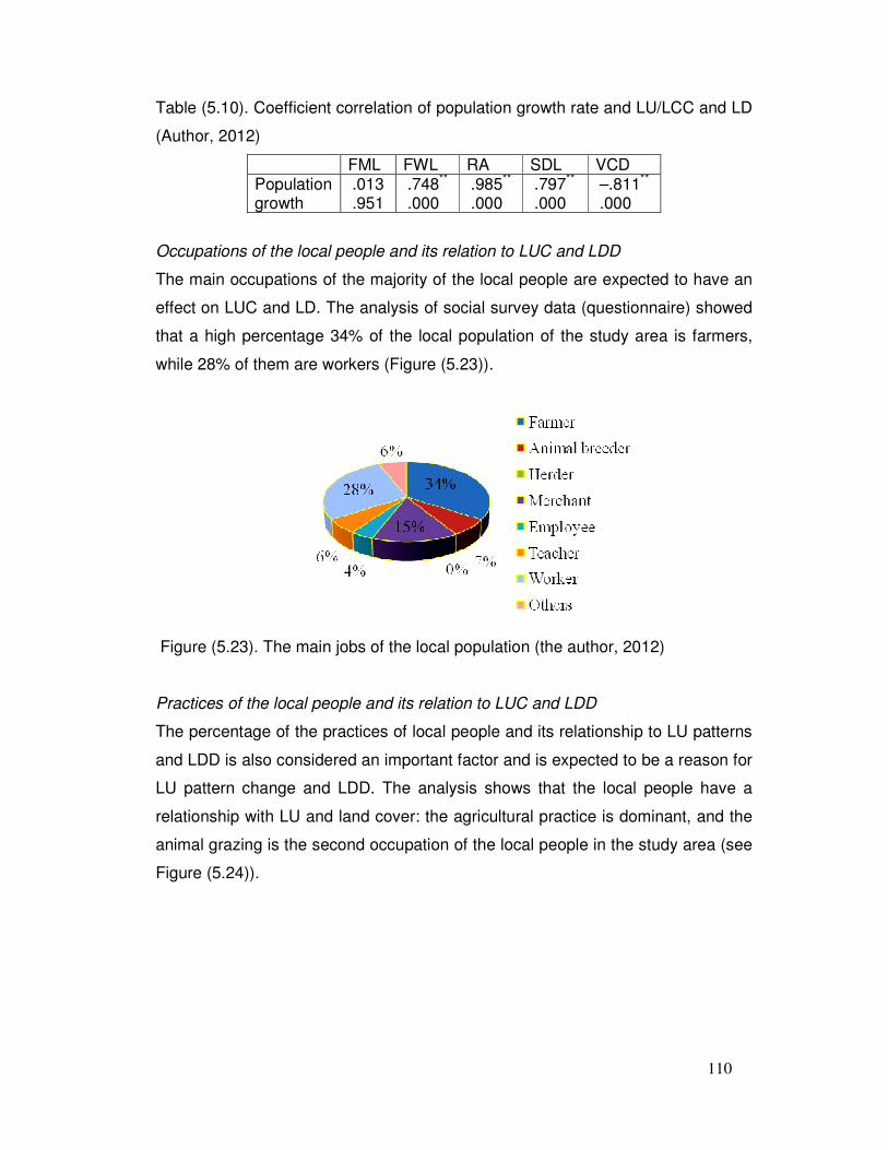
110
Table (5.10). Coefficient correlation of population growth rate and LU/LCC and LD
(Author, 2012)
FML FWL RA SDL VCD Population growth
.013
.951 .748** .000
.985**
.000 .797** .000
–.811** .000
Occupations of the local people and its relation to LUC and LDD
The main occupations of the majority of the local people are expected to have an
effect on LUC and LD. The analysis of social survey data (questionnaire) showed
that a high percentage 34% of the local population of the study area is farmers,
while 28% of them are workers (Figure (5.23)).
Figure (5.23). The main jobs of the local population (the author, 2012)
Practices of the local people and its relation to LUC and LDD
The percentage of the practices of local people and its relationship to LU patterns
and LDD is also considered an important factor and is expected to be a reason for
LU pattern change and LDD. The analysis shows that the local people have a
relationship with LU and land cover: the agricultural practice is dominant, and the
animal grazing is the second occupation of the local people in the study area (see
Figure (5.24)).
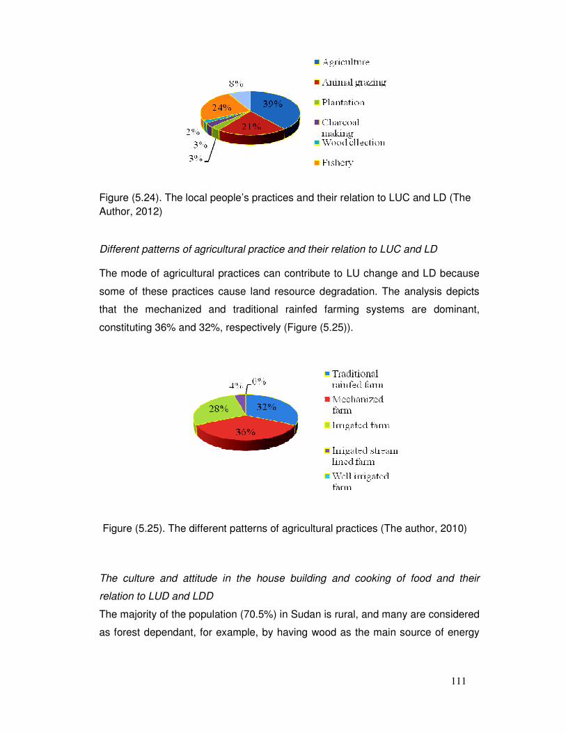
111
Figure (5.24). The local people’s practices and their relation to LUC and LD (The Author, 2012)
Different patterns of agricultural practice and their relation to LUC and LD
The mode of agricultural practices can contribute to LU change and LD because
some of these practices cause land resource degradation. The analysis depicts
that the mechanized and traditional rainfed farming systems are dominant,
constituting 36% and 32%, respectively (Figure (5.25)).
Figure (5.25). The different patterns of agricultural practices (The author, 2010)
The culture and attitude in the house building and cooking of food and their
relation to LUD and LDD
The majority of the population (70.5%) in Sudan is rural, and many are considered
as forest dependant, for example, by having wood as the main source of energy
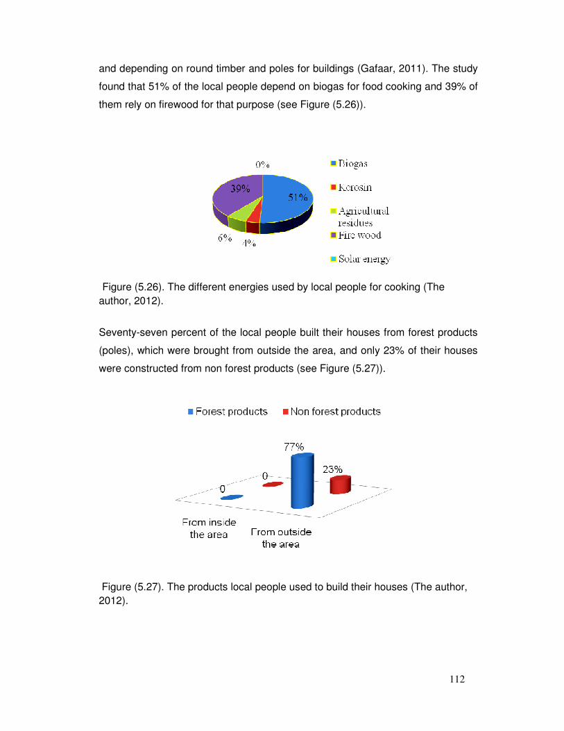
112
and depending on round timber and poles for buildings (Gafaar, 2011). The study
found that 51% of the local people depend on biogas for food cooking and 39% of
them rely on firewood for that purpose (see Figure (5.26)).
Figure (5.26). The different energies used by local people for cooking (The author, 2012).
Seventy-seven percent of the local people built their houses from forest products
(poles), which were brought from outside the area, and only 23% of their houses
were constructed from non forest products (see Figure (5.27)).
Figure (5.27). The products local people used to build their houses (The author, 2012).
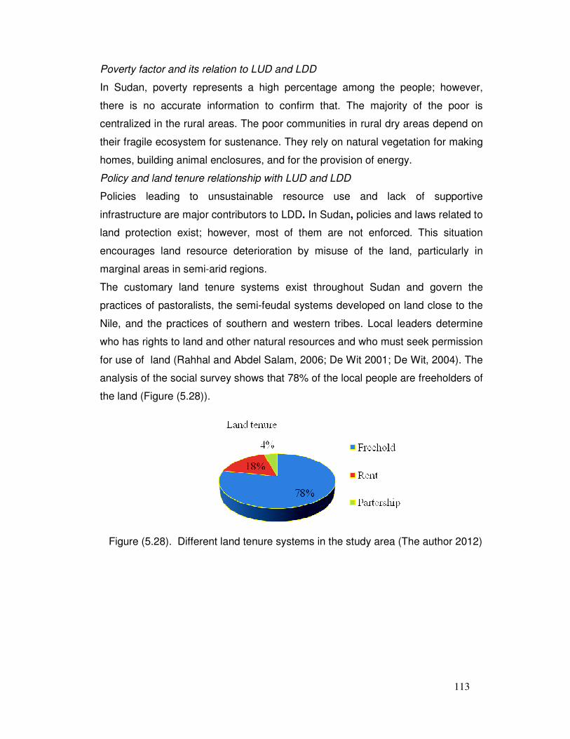
113
Poverty factor and its relation to LUD and LDD
In Sudan, poverty represents a high percentage among the people; however,
there is no accurate information to confirm that. The majority of the poor is
centralized in the rural areas. The poor communities in rural dry areas depend on
their fragile ecosystem for sustenance. They rely on natural vegetation for making
homes, building animal enclosures, and for the provision of energy.
Policy and land tenure relationship with LUD and LDD
Policies leading to unsustainable resource use and lack of supportive
infrastructure are major contributors to LDD. In Sudan, policies and laws related to
land protection exist; however, most of them are not enforced. This situation
encourages land resource deterioration by misuse of the land, particularly in
marginal areas in semi-arid regions.
The customary land tenure systems exist throughout Sudan and govern the
practices of pastoralists, the semi-feudal systems developed on land close to the
Nile, and the practices of southern and western tribes. Local leaders determine
who has rights to land and other natural resources and who must seek permission
for use of land (Rahhal and Abdel Salam, 2006; De Wit 2001; De Wit, 2004). The
analysis of the social survey shows that 78% of the local people are freeholders of
the land (Figure (5.28)).
Figure (5.28). Different land tenure systems in the study area (The author 2012)
114
Chapter Six
Discussion
The chapter reviews the discussion of the important findings of the assessment of
impacts of the changes in the land use patterns change (LUC) on land
degradation and desertification (LDD) in the dry land.
6.1 Assessment of LDD
The assessment based on vegetation cover degradation (VCD) and soil
degradation (SDL) based on sand dunes movement and accumulation:
A) The findings depicted SARVI as a more appropriate vegetation index (VI)
than NDVI, SAVI, ND2-25, and ND42-57 for assessing the LDD based on the
vegetation degradation indicator in the semi-arid zone. The produced map of
SARVI indicated that the vegetation cover, slightly corresponded to the ground
truth of study area (Figure (5.1)), and that this might attribute to its development
(Kaufman and Tanre, 1992). It was improved for removing the influence of
aerosols through the use of the blue band (B) (the most sensitive to atmospheric
haze) to correct aerosol effect on the red band, as well as to reduce soil noise.
Therefore, SARVI can be used efficiently in arid and semi-arid environments of
the Sudan, where sparse annual and perennial vegetation dominates; it is a new
application in the study area. However, SARVI is not applicable with all imageries
of sensors that do not contain the blue band; e.g., MSS and ASTER. Thus, the
application of SARVI is restricted in TM and ETM images, so in this case, it is not
better than NDVI and SAVI, which can be applied to most of the sensors easily.
ND2-25 and ND42-57 applications were adopted for the first time in the semi-arid
environment. Their maps indicated the vegetation cover and other features in dark
colour (minus value) except the sand and sand dunes (plus value). Accordingly,
they are not efficient and suitable VIs for the dry land, although some studies
stated that ND2-25 and ND42-57 have a higher correlation coefficient with forest
stand attributes (such as biomass, volume and average stand diameter) than the
indexes that not contain band 5, such as NDVI (Liu et al., 2004).
With regard to the assessment of the vegetation degradation, the resulting SARVI
map illustrated that severe VDC dominates and is distributed widely in the central
115
part of the area, attributed to the existence of sparse herbaceous plants, grasses,
and scattered shrubs growing on fragile sand soil. The land is used as range land
for livestock of local people. Thus, overgrazing has contributed to that condition.
The important result that the trend of the sever VDC area increased slowly over
1986 and 2010 (Figure (5.4)) due to degradation of the herbaceous and shrubs on
account of the animal grazing; however, it was not the unique reason. Many
factors are existed, and they are discussed in the next subchapter (causative
factors of LUC and/or LDD in the study area). The severe degradation of
vegetation cover was not large in that period because there was an increase in
the area of intact and light degradation (very dense and dense vegetation) that
might be attributed to the spreading of Mesquit (Prosopis pubescens) plants,
which was remarkable. This plant is characterized by rapid spreading, and
currently has been causing deterioration in the agricultural land of the local
people; they have been suffering from its spread.
B) Assessment of soil degradation by using GSI: the produced GSI map
showed that both the severe and very severe soil degradation represent 22% of
the whole study area. The very severe soil degradation (active sand dunes) is
distributed in different areas and represents 6%, and the severe soil degradation
represents 16%, covering a large area (Figure (5.8)). Over 1986–2010, the area of
very severe soil degradation (active sand dunes) increased by 69.5 Km2, about
2.9 Km2 per annum, while the area of severe soil degradation (inactive),
decreased 73 Km2 through 24 years and 3 Km2 annually. The increase in the area
of very severe soil degradation land (active sand dunes) indicates that
degradation of vegetation happened, followed by wind erosion, causing activation
of fixed sand (severe soil degradation) due to numerous factors, such as human
activities and shortage of the rainfall. More clarification of these factors is given in
the results regarding impacts of LU patterns (human activities) on LDD and
analysis of driving factors of LUC and/or LDD.
116
6.2. Assessment of land use change (LUC) impact on degradation and
desertification (LDD) by using pixel based image analysis (PBIA) and object
based image analysis (OBIA) approach:
1) Comparison between PBIA and OBIA for assessing LUC land
degradation and desertification and LDD
According to the accuracy and efficiency assessment results, the OBIA-fuzzy logic
classifier was selected instead of the PBIA-hybrid classification likelihood classifier
for mapping and assessing LU pattern change and its effects on LDD. The
accuracy assessment process for the two methods revealed no significant
difference between them. The overall accuracy of OBIA equals 87.4 and PBIA
equals 87; however, OBIA is slightly more efficient because it allows for
successful delineation of the RAs among the other classes, which is difficult to
achieve by using PBIA due to similarity of signature of RAs with signatures of
other classes, e.g., fallow land, semi-bare land. The OBIA-fuzzy logic approach
allowed for the categorization of the LU and LDD into eight classes (Figure (5.10)
and Tables (5.3) and (5.4)).
2) Spatiotemporal trend of the LU Classes (patterns) and LDD in the
periods 1973–1986 and 1986–2009
Changes in the LU/LDD categories occurred in the periods of 1973–1986 and
1986 – 2009. The period 1973 to 1986 illustrated obvious changes in the different
LU classes and vegetation and soil categories, leading to an increase in the areas
of dense wood (DWL), residential (RA), and fallow land (FWL), as well as water
body, while leading to a decrease in the areas of severe degrading land (SDL),
mixed range land (MRL), farm land (FML) and mixed vegetation land (MVL).
Likewise the period of 1986–2009 witnessed an increase of areas of RA, SDL,
MRL, and FML, and a decrease in the areas DWL, FWL, and MVL (see Figure
(5.17)). No doubt, a synergism of several causing factors account for the LU
pattern changes and LD. Therefore, the study addressed and analysed some
hypothetical causing factors of LU patterns change and/or LD. Those changes in
LU patterns play an effective role in the acceleration of LD trends.
3) Effects of LU patterns change on LDD
A) Effects on the vegetation cover degradation (VCD)
117
The LU patterns change occurred in 1973–1986 and 1986–2009 affected different
types of the CV (DWL, MRL, and MVL). Apparently, the RA, FML, and FWL
affected DWL, MRL, and MVL (Figure (5.13)). Particularly FML and FWL were
strongly affected by or contributed to the DWL, MRL, and MVL degradation,
leading to a decrease in DWL, MRL, and MVL areas over 1973–1986 (Table
(5.5)). This was due to the intensive agricultural activities in the area, referring to
demographic factors, because during that period, some parts of Sudan were
affected by drought and famine, leading to the displacement of a great number of
the people from western Sudan (Kordofan and Darfur), and their subsequent
settling in the central regions, specifically in the Elgeteina locality. Dramatic
change in LU took place during that period: 85.9 Km2 of MVL converted to FWL
because those areas witnessed the establishment of a big agricultural scheme,
which led to the removal of the whole MVL.
In 1986–2009, the LU change affected the vegetation cover types: 15 Km2 of the
DWL area changed into the LU classes. The FWL had more of an effect on DWL,
expanding 9.6 Km2 at the expense of DWL, and 18.1 Km2 of the MRL area
converted to FML and FWL (Figure (5.14)). During both periods, the agricultural
LU activities had more effect on the vegetation cover types. This result
corresponded to the activities of the local people, as most of them are practicing
agricultural activities (39%), and more than 50% of the population are practicing
agriculture. This result also confirms the study hypothesis that agriculture causes
LDD; particularly, the vegetation degradation in the semi-arid area of the Sudan is
much more severe than other LU activities.
The above discussions regard the impacts of LU change on the vegetation pattern
degradation. However, other land cover patterns also contributed to the vegetation
condition of the study area during 1973–1986 and 1986–2009. Appendices (9),
(10), (11), and (12) give the full picture of the mutual conversion processes, which
led to the LU and land cover (LD) dynamic trend illustrated in Table (5.5).
B) Effects on the soil degradation
The LU classes change affected soil degrading land (SDL) slightly from 1973–86
and 1986–2009. The spatiotemporal change of the LU classes affected the sand
and sand dune movement slightly: 0.4 Km2 of the FWL and FML changed into
118
SDL or moving sand dunes, and 2.6 Km2 of the SDL converted to RA, FWL, and
FML. In general, it is noted that the mutual impact that took place between the LU
classes and soil degrading land patterns was not large, because the LU activities
were in the areas of clay soil (see Figure (5.15)). In 1986–2009, 2.3 km2 of the
SDL area changed into RA, FWL, and FML. It is noted that a small increase
occurred in the areas of SDL at the expense of areas of the RA and FWL from
1986–2009, compared with the period of 1973–1986, due to the continued status
of LU pattern changes (Figure (5.16)).
Likewise, other land cover classes affecting LDD led to the sand dunes dynamic in
1973–1986 and 1986–2009 (Figures (5.13) and (5.14)).
3) Modelling the influence of LU patterns change on LD A) Modelling the LU patterns affecting vegetation cover degradation
The results of the multi-linear regression analysis for building models of the impact
of LU change on the VCD were as follows:
The FWL and RA formed the model and are associated with vegetation cover.
They have become the predicted factor of vegetation cover degradation. RA has
more effect on VCD than FWL, where 1 unit increase in RA leads to a 3.357 unit
decrease in the VCD area, meaning the vegetation cover degradation links with
the expansion of the settlement and the growth of the population, as well as the
agriculture.
B) Modelling the LU patterns affecting soil degradation land (SDL)
The produced a model of LU patterns affecting SDL:
The FML and FWL were the predicted and controlling factors of soil degradation.
FML has more influence on SDL than FWL. A 1 unit increase in the FML area
leads to a 0.623 unit increase in the SDL area. Therefore, SDL has a link with
agricultural LU activities.
The checking assumptions were carried out for the two models. The
multicollinearity checking was done, showing no high correlation (> 0.9) existed
between the independent variables; therefore, no variable was excluded.
4) Driven factors of LU change and/or LDD and LDD in the study area
A) The impact of climate variability on LU patterns and/LDD
119
The climate elements variability showed a weak correlation with LU patterns,
consequently its contribution to the changes in LU patterns is poor. However,
those results do not exclude the impact of some climate elements on LU patterns,
particularly the rainfall factor. Although the weak rainfall has effects, big changes
in agricultural LU occurred during that period, because most of the agricultural
activities depend on the irrigation system on the White Nile. As the correlation of
climate elements variability with LD (vegetation and soil degradation) was
insignificant, likely it had a slight role in the LDD during 1973–2009. However, the
scarce rainfall might have a significant role in LDD in the drought period that hit
the area in 1973–1986, particularly in 1984, which was catastrophic.
A) Indirect human inducing factors of LU patterns change and/or LDD
The social survey analysis showed that socioeconomic status has a role in the
LUC and/or LDD: the majority of the local people of the study area are farmers:
34%, with about 39%, and 24% of those practicing agricultural and animal herding
activities, respectively. The dominant agricultural system is mechanized farm,
representing 36%, in addition to the traditional rainfed and irrigated farms
representing 32% and 28%, respectively. During the study period, some changes
occurred in local peoples’ attitudes in utilizing energy in cooking food where that
51% and 39% utilized biogas and firewood in cooking food, respectively.
Moreover, the population growth had correlation with all LU patterns, ranging from
a medium to very strong correlation. It also had a medium to strong correlation
with the indicators of LDD (soil and vegetation degradation). Apparently those
results indicate that the population growth rate and the socioeconomic status of
the local people relating to LU activities and natural resources play a big role and
contribute to the status of the changes in LU patterns and LDD. However, after
refining for oil in the Sudan, changes in the attitudes of local people in utilizing
energy to cook food took place. They have become dependent on biogas more
than firewood. This change will reduce the pressure on the tree and shrub cover in
the area.
120
Chapter Seven
Conclusions, Recommendations, and Outlook
The chapter reviews the conclusions of the important findings in this study,
addresses the important recommendations, and gives the outlook.
Conclusions
The conclusions of the study regarding assessment of the impacts of the changes
in LU patterns on LDD, in general this study is considered new idea and also the
methodology which was applied is novel in the study area, in details the study
concludes as follows:
• SARVI proved to be slightly more efficient than NDVI, SAVI, ND4-25, and
ND42-57 for assessing vegetation degradation in semi-arid areas; it was able to
indicate some sparse vegetation not clear in the other indexes by its overcoming
soil background and atmospheric factors.
• GSI proved high efficiently in determining the different types of soil
degradation and in producing the map of top soil grain size that assisted in the
assessment of LDD.
• OBIA-fuzzy logic classification achieved a higher performance than the
PBIA-hybrid classification for image analysis for assessing LU patterns impact on
LD. However, its processes of the LU and LDD classification are more time
consuming than the other method.
• The trend of LDD in semi-arid areas is increasing annually, as assessment
of vegetation and soil degradation indicators illustrated. This result agrees with the
hypotheses (1).
• Four status of LU and land cover dynamic changes took place during
1973–1986 and 1986–2009:
1. RA had an increased changing trend
2. MVL had a decreased changing trend
3. DWL and FWL had an increased and decreased changing trend
4. SDL, MRL and FML had a decreased and increased changing trend
• Apparently, the changes in LU patterns (RA, FWL and FML) that took
place in 1973–1986 and 1986–2009, affected different patterns of the vegetation
121
cover (DWL, MRL and MVL). MVL was influenced by FWL dramatically, causing
removal of 85.9 Km2 of MVL, attributing to the establishment of agricultural
schemes in that area during 1973–1986. FWL greatly influenced MRL during
1986–2009.
• The LU patterns change also affected soil degradation, which led both to
the slow movement of sand dunes and to the sand dune fixation in the adjacent
area to the LU activities during 1973–2009.
• Remarkably, the agricultural activity among the other LU was the dominant
and had more effect on LDD, particularly, on the vegetation cover degradation.
• There was fusion of RS data with socioeconomic and climatic data to
create correlations and valid models of the impact of LU classes (patterns) on
LDD in the semi-arid zone at the spatiotemporal scale, by adopting the statistical
analysis, namely Pearson coefficient correlation and multi-linear regression.
• According to the medium-strong correlation of the population growth with
the LU patterns change and the critical portion of socioeconomic of the local
people related to LU patterns activities and moreover, the different agricultural
system followed in the study area, those factors contributed to or caused the
changes in LU patterns and LDD. While the effects of climate elements variability
in LU patterns change and/or LDD were slight, nevertheless the rainfall variability
had some effects and medium correlation with the vegetation cover.
Constraints
• No availability of the imagery for specific time and date or to cover a certain
area
• Inapplicability of some vegetation and soil indices on the imagery of all
sensors
• No availability of old historical maps and aerial photography for the study
for the validation and accuracy assessment processes.
Recommendation
After the theoretical data, the application processes of the different techniques for
performing the objectives, extraction, and discussion of the valuable information
regarding LU patterns changes and their impacts on LDD, this type of the study
122
has become obviously very critical and important research in the semi-arid and
marginal areas for determining the interaction between the human being activities
and his environment and how to apply the developed methods such as remote
sensing technology and GIS in these aspects to create environmental balance
and to solve and avoid occurrence of such as desertification processes, climate
change and other environmental problems, therefore study recommends with
important things through the achievements of this novel research in the study area
as :
• Application of SARVI on the vegetation study in the dry land. In this case,
the study was restricted in the use of TM and ETM sensor images, which were
slightly more efficient than using NDVI and SAVI.
• Using GSI in assessing soil degradation and LDD. It has an ability to
determine the top grain soil of surfaces, particularly in determining sand and dune
habitats.
• The application of OBIA-fuzzy logic in the study of LU patterns and LDD in
dry land has a better performance than PBIA, particularly in the case of using
images in medium and high resolution.
• Such as this assessment, the analysis and modelling of the LU patterns
change and their relationship to LDD are the most critical parameters in dry land
to be recommended, particularly in the Sudan.
• Replication of this study by using different imagery with high resolutions
and sophisticated software, such as eCognition and Feature Analyst (FA) for
increasing the validity and accuracy of the assessment and modelling of LU
patterns and LDD status in dry land is important in the Sudan.
• More researches are required for finding efficient VIs thoroughly applicable
on the imagery of all sensors and at the same time, that are more resistant to the
effects of atmosphere and soil reflection and able to detect and determine the
sparse vegetation cover of dry land.
Outlook
Through application of this research in the study area appeared many outlooks of researches will get done in the future as follows:
123
• Modelling-based assessment of soil degradation dynamic and its
relationship to the LU patterns/land cover dynamic and climate change in
dry lands of the Sudan by using advanced RS technology.
• Mapping and modelling of vegetation degradation dynamic and its impact
on climate change in the dry lands of the Sudan by using advanced RS
technology.
• Detecting and predicting impacts of LDD on carbon sequestration in the dry
lands of the Sudan by using advanced RS technology.
• Monitoring the sand dunes dynamic and its threat to the agroecosystem in
the dry lands of the Sudan by means of sophisticated RS and GIS.
124
Cited literature
Abbadi, K.A.B and Ahmed, A.E. 2006. Brief overview of Sudan economy and
future prospect for agriculatural development. Khartoum Food aid 2006.
Retrieved on the 18th of April 2007 from
http://nutrition.tufts.edu/pdf/research/famine/publications/foodaid2006/suda
n economy and agricultural development pdf.
Adeel, Z., Safriel, U. Niemeijer, D. and R. White. 2005. Ecosystems and Human
Well-Being: Desertification Synthesis, World Resource Institute,
Washington, D.C.
Akatar-Schuster, M., Bigas, H., and Thomas, Richard. 2009. Monitoring and
Assessment of Desertification and Land Degradation: Knowledge
Management, Institutions and Economics, UNU Desertification Series No.
9.
Amarsaikhan, D. 2010. Fusing High- resolution SAR and Optical imagery for
improved urban land cover study and classification. Int J Image Data
Fusion 1:83.
ASPRS, 1994. Remote Sensing and Geographic Information System: An
integration of Technologies for resource management (Bethesda, MD:
ASPRS).
Aubreville, A. 1949. Climats, Forest et Desertification de Afrique Tropcale. PARIS:
Geogr. Marit and Col., 351p.
Ayoub A.T. 1998. Extent, severity and causative factors of land degradation in
Sudan. Journal of Arid Environments 38: 397-409.
Balba, M.A. 1995. Management of problem soils in arid ecosystems. Boca Raton,
FL: CRC Lewis Publishers. 179-239 pp.
Bannari, A. 1995. A review of vegetation indices. Remote Sens Rev 13:95.
Baret, F., Guyot, G., and Major D. J. 1989. TSAVI: a vegetation index, which
minimizes soil brightness effects on LAI and APAR estimation. In:
Proceedings of the 12th Canadian Symposium on Remote Sensing,
IGARRSS’90. Vancouver BC, Canada, 10-14 July, Volume 3.
125
Benz, U., Hofman, P., Willhouk, G., Lingenfelder, I and Heynen, M. 2004. Multi-
resolution, Object-oriented fuzzy analysis of remote sensing data for gis-
ready information. ISPRS Journal of photogrammetry & Remote Sensing
58 (2004), 239-258.
Bilotta. G.S., Brazier RE and Haygarth PM. 2007. The impacts of grazing animals
on the quality of soils, vegetation, and surface waters in intensively
managed grasslands. Advances in Agronomy 94: pp 237-279.
Bitelli, G., Camassi, R., Gusella, R., and Mongol, A. 2004. Image change
detection on urban area: The earthquake case. Proceedings of the ISRPS
2004 Annual Conference, Istanbul, Turkey. July 19-23.
Blaschke, T. 2005. A framework for change detection based on image objects. In:
Göttinger Geographiche Abhandlungen, S., Erasmi, B., Cyffka, M. Kappas,
(Eds.) 113, 1-9. Goltze, Goettigen.
Blascke T. 2009. Object based image analysis for remote sensing, ISPRS Journal
of Photogrammetry and Remote Sensing, journal homepage:
www.elsevier.com/locate/isprsjprs
Blascke T. 2010. Object based image analysis for remote sensing, ISPRS Journal
of Photogrammetry and Remote Sensing, 65: 2-16.
Bolle, H. J. 1994. Remote sensing in desertification studies. In Desertification in
an European context- Physical and socio-economic aspects. Report EUR.
15415.
Borengasser, M., Hungate, W.S and Watkins, R. 2008. Hyperspectral Remote
Sensing, Principles and applications. ISBN 978-1-56670-654-4. CRC
press/Taylor & Francis Group.
Braimoh, A. K., and Vlek, P.L.G. 2004. The impact of land-cover change on soil
properties in northern Ghana. Land Degrada-
Brico, B., and Brown, R. J. 1995. Multidate SAR/TM synergism for crop
classification in western Canada. Photogram Eng Remote Sens 61:1009.
Brunce, J. 1993. The variety of reform: A review of recent experiences with land
reform and the reform of land tenure, with particular reference to the Africa
experience. In: Marcussen, H:S. (ed.) Institutional issues in natural
126
resource management. Denmark: International Development Studies,
Roskilde University.
Byun, Y.G., Han, Y.K. and Chae, T.B. 2013. A multispectral image segmentation
approach for object-based image classification of high resolution satellite
imagery, 486, KSCE Journal of Civil Engineering (2013) DOI
10.1007/s12205-013-1800-0.
Cabral, P., Gilg, J., and Painho, M. 2005. Monitoring urban growth using remote
sensing, gis and spatial metrices, remote sensing and modeling of
ecosystems for sustainability. Proceedings of SPIE – Optics & Photonics,
San Diego.
Campbell, J. B. 1996. Introduction to Remote Sensing. New York: Guilford Press.
Caprioli, M., Tarantino E., 2003. Urban features recognition form VHR satellite
data
Caselles, V. And Garica, M. J. L. 1989. An alternative simple approach to estimate
atmospheric correction in multitemporal studies, International Journal of
Remote Sensing, Vol. 10, 1127-1134.
CBS, 2005. Central Bank of Sudan 45th annual report 2005. Retrieved on the 18th
of April, 2007 from http://www.bankofsudan.org.
Chandra, m., Moreira, A., and Keydel, W. 2005. Amper: Network on applied
multiparameter environmental remote sensing. An eu sponsored research
and training network. Proceedings of the IGARSS 2005 Symposium. Seoul,
korea.
Chavez, P. S. Jr. 1996. Image-based atmospheric correction – revisited and
improved, Photogrammetric Engineering and remote sensing, Vol. 62, n. 9,
1025-1036.
Chen, D., and Stow, D. A. 2003. Strategies for integrating information from
multiple spatial resolution into land- use/land-cover classification routines.
Photogram Eng Remote Sens 69:1279.
Chunyan, H., Li, J., Zhang., Pan, Y., and Chen, Y. H. 2005. Dynamic monitor on
urban expansion based on a object-oriented approach. Proceeding of the
IGARSS 2005 Symposium. Seoul, Korea, 25-29 July.
127
Chuvieco, E. 2008. Earth Observation of Global Change (The Role of Satellite
Remote Sensing in Monitoring the Global Environment) Springer.
Chuvieco, E. and Heute, A. 2010. Fundamental of Satellite Remote Sensing.
ISBN 978-0-415-31084-0.CRC Press/Taylor& Francis Group.
Clarke and Noin 1998. In: J. Clarke and D. Noin, Editors, Population and
environment in arid regions, UNESCO/Partenon Publishing Group, Paris,
pp. 1-18
Congalton, R. G and Mead, R.A. 1983. A quantitative method to test for
consistency and correctnessin photo interpretation. Photo program Eng
remote Sens49:69.
Congalton, R. G. 1991. A review of assessing the accuracy of classification of
remotely sensed data. Remote Sens Environ 37:35.
Congalton, R. G. and Green, K. 2008. Assessing the accuracy of remotely sensed
data. Remote Sens Environ 37:35.
Congalton, R. G. and Plourde, L. 2002. Quality assurance and accuracy
assessment of information derived from remotely sensed data. In Manual of
Geospatial Science and Technology, ed. J. Bossler, 349. London Taylor &
Francis.
Courel M.F., Kandel R.S. and Rasool S. I. 1984. Surface albedo and the Sahel
drought, Nature, Vol. 307, 528-531.
Cracknell, A.P. and Hayes, L. 2007. Introduction to Remote Sensing, Second
edition, ISBN- 10: 0-8493-9255-1 (hardback). CRC press/Taylor & Francis
Group. Cambridge University Press.
Crase, B. and Hempel, C. 2005. Object based land cover mapping for groote
eyland: a tool for reconnaissance and land based surveys. Proceedings of
NARGIS 2005 – APPLICATIONS IN TROPICAL SPATIAL SCIENCE. 4th-
7th July Charles Darwin University, Darwin, NT, Australia.
Crist, E. P. and Cicone, R. C. 1984a. Application of the Tassel Cap concept to
simulated Thematic Mapper data, Photogrametric Engineering and Remote
sensing, Vol. 50, 343-352.
128
Crist, E. P. and Cicone, R. C. 1984b. A physical based transformation of thematic
mapper data- The tasseled cap, IEEE Transaction on Geoscience and
remote sensing, Vol. GE22, n. 3, 256-263.
Csaplovics, E. 1992. Methoden der regionalen Fernerkundung, Anwendungen im
Sahel Afrikas.
Cushnie, J. L. 1987. The Interactive effect of spatial resolution and degree of
internal variability within land-cover types on classification accuracies.
International Journal of Remote Sensing, 51-1483.
Dai, X and Khorram, S. 1998. A hierarchical methodology framework for
multisource data fusion in vegetation classification. Int J Remote Sens
19:3697.
Darvish, A., Leukert, K., and Reinhardt, W. 2003, Urban land-cover classification:
an object based perspective. In 2nd GRSS/ISPRS Joint Workshop: Remote
Sensing and Data Fusion over Urban Areas, 22-23 May, Berlin, pp. 278-
282.
Dave, J. V. 1980. Effect of atmospheric conditions on remote sensing of a surface
of non-homogeneity, Photogrammetric Engineering and remote sensing,
Vol. 46, 1173.
Davis, D.K. 2004. Desert ‘wastes’ of the Maghreb: desertification narratives in
French colonial environmental history of North Africa. Cultural Geographies
pp 11: 359
De Jong-Boon, Caroline, (1990). Environmental Problems in the Sudan, Part I, The Hague.
DECARP, 1976. Desert Encroachment Control and Rehabilitation Programme.
Denti, G.D. 2004. Developing Desertification Indicator System for A small
Mediterranean Catchment: A case Study From The Serra De Rodes, Alt
Emporda, Catalunya, Ne Spain. A thesis. Pp 35
D-JAM. 2006. Republic of the Sudan: status of natural resources and
Environment. Darfur Joint Assessment Mission. Retrieved on the 20th of
April, 2007 from
http://www.unsudanig.org/darfurjam/trackII/data/preliminary/development/St
129
atus%20of %20Natural%20Resources%20and%20the%20Environment-
%2024th%20August.doc.
Dregne, H. E., Kassas, M. and Rozanov, B. 1991. A new assessment of the world
status of desertification. Desertification Control Bulletin, 20, 6 – 19.
Dregne, H.E. 1976. ´´Desertification: Symptom of a Crisis.´´ In Handbook of
Desertification Indicators, ed. Reining, P., AAAS, Washington D.C., 141p.
Dregne, H.E. 1986. ´´Desertification of Arid Lands´´. In Physics of Desertification,
ed. F. El-Baz and M.H.A. Hassan, Dordrecht, The Netherlands: Martinus,
Nijhoff. Dregne. H. E.,
Drewry J.J., Cameron, K.C. and Buchan G.D. 2008. Pasture yields and soil
physical property responses to soil compaction from treading and grazing:
a review. Australian Journal of Soil Research 46, 237–256.
Duda, R. O., Hart, P. E., and Stork, D.G. 2001. Paterrn classification, New York:
John Willy & Sons, 654p.
Ecognition, 2001. Function Guide
Eden Foundation, 1994. ´´ Desertification- A threat to Sahel´´. www.eden-
foundation.org, 9 p.
Ehleringer, J. R. and Björkman, O. 1978. Pubescence and leaf spectral
characteristics in a desert shrub, Encilia forinosa, Oecologia, 36: 151-162.
Elers, M.. 2010. Multisensor image fusion for pansharpening in remote sensing.
Int J Image data fusion 1:25.
Elfadl, M.A. 1997. Management of Prosopis juliflora for Use In Agro-forestry
System in Sudan PhD.D. Thesis, University of Helsinki.
Ellis, E. 2010. Land use and land cover change, Natural science, retrieved 4/2011
<http://www.eoearth.org/article/Land-use>.
Elmoula, M. E. A. 1985. On the problem of resource management in the Sudan.
Monograph Series No. 4, Institute of Environmental Studies, University of
Khartoum. 131 p.
Elmqvist, B. 2006. Livehood diversification and land use in the Sahel: an
interdisciplinary analysis o s Environment Programme. 14 p.
130
Elsiddig, E.A. 2004. Community Based Natural Resource Management in Sudan,
In: Awimbo, J., Barrow, E and Karaba, M. 2004. Community Based Natual
Resource Management in the IGAD region. IGAD; IUCN.
Emadodin, I., Reiss, S., Mitusov, A. V. & Bork, H. R. 2009. Interdisciplinary and
multidisciplinary approaches to the study of long-term soil degradation: A
case study from Schleswig-Holstein, Germany. Land Degradation &
Development
English, C., Richards, T. S., and Moheidin, Y. E. 1997. GIS and remote sensing
applications to desert margin vegetation and land use monitoring in
Sahelian Sudan: methodology, data integration problems, and solutions: in
McGinty (ed.) International Symposium and Workshop on Combating
Desertification: Connecting Science with Community Action, Tucson,
Arizona, USA.
Engvall, J. L., Tubbs, J.D. and Holmes, Q. A. 1977. Pattern recognition of Landsat
data based on temporal trend analysis, Remote Sensing of Environment,
Vol. 4, 31-32.
Enne, G. and Zucca, C. 2000. Desertification indicators for Europian
Mediterraneam region, State of the art methodological approaches. ANPA
and ARD. Printed by Sped Srl – Rome (Italy).
Erle, E and Robert, P. 2010 .Land-use". In: Encyclopedia of Earth. Eds. Cutler J.
Cleveland (Washington, D.C.: Environmental Information Coalition,
National Council for Science and the Environment). [First published in the
Encyclopedia of Earth August 6, 2010; Last revised Date August 6, 2010;
Retrieved http://www.eoearth.org/article/Land-use
Escadefal, R., Girard, M. C. and Courault, D. 1989. Munsell soil color and soil
reflectance in the visible spectral bands of Landsat MSS and TM data.
Remote Sens. Environ. 27:37-46.
Eswaran, H.,. Lal, R and Reich. P.F. 2001. Land degradation: an overview. In:
Bridges, E.M., I.D. Hannam, L.R. Oldeman, F.W.T. Pening de Vries, S.J.
Scherr, and S. Sompatpanit (eds.). Responses to Land Degradation. Proc.
2nd. International Conference on Land Degradation and Desertification,
131
Khon Kaen, Thailand. Oxford Press, New Delhi, India F gum Arabic in
Sudan. Lund University, Lund, Sweden.
Fadol, W., Salih. M., Elhag A. M. H. and Hamid.A.A. 2012. Assessment of sand
ncroachment in El-Qutaynah area, Sudan using remote sensing and
geographic information system. Journal of Soil Science and Environmental
Management Vol. 3(5), pp. 97-103.
FAO 2005, AGRO-ECOLOGICAL ZONING AND GIS APPLICATIONS IN ASIA -
with special emphasis on land degradation assessment in drylands (LADA).
Proceedings of a Regional Workshop Bangkok, Thailand 10–14 November
2003, AGL/MISC/38/2005.
FAO, 1995a. Prevention and disposal of obsolete and unwanted pesticide stocks
in Africa and the Near East. Rome, Food and Agriculture Organization
FAO, 1997. Land quality indicators and their use in sustainable agriculture and
rural development. FAO Land and Water Bulletin 5, 212 p.
FAO, 2001b. State of the world’s forests. FAO, Rome.
FAO. 1996. Forest Resources Assessment 1990. Survey of Tropical Forest
Cover and Study of Change Processes. FAO Report 130, Food and
Agriculture Organization of the United Nations, Rome, Italy, 152 pp.
FAO. 2001a. Global forest resources assessment 2000. Main report. FAO
Forestry Paper NO. 140. Rome.
FAO/UNEP, 1999. The Future of our land: facing the challenge. Guidelines for
integrated planning for sustainable management of land resources. 71 p.
FAO/UNEP. 1984. Map of Desertification hazards: explanatory note. Nairobi,
Kenya: United Nation.
FAO/UNEP/UNESCO, 1979. Provisional Methodology of Soil Degradation
Assessment; 73 p.
Foody, G. M. 2002. Status of land cover classification accuracy assessment.
Remote Sens Environ 80 :185.
FRA. 2010. The global land-use change emission is approximately equal to the
tropical land-use change emission because the net carbon balance of land
-use changes in temperate and boreal regions is neutral (Houghton, 2003,
2007) (24, 26).
132
Fu, H., Wang, Y., Wu, C and Ta L. 2002. Effect of grazing on soil physical and
chemical properties of Alxa desert grassland. J. Desert Res. 22:339-343.
Gaiballah, A K., and Farah, A M. 2004. A proposed plan for research in
desertification in Sudan : White Nile State, Proceeding in the National
Forum of Scientific Research on Desertification on Sudan, 2004, University
of Khartoum,
Gamba, P. and Herold, M. 2010. GLOBAL MAPPING OF HUMAN SETTLEMENT,
Experiences, Datasets, and Prospects. Toylor & Francis Series in Remote
Sensing Applications.
Gao, J. 2009. Digital analysis of remotely sensed imagery. New York, The
McGraw-Hill Companies, Inc.
Gao, J., Zha Y and NI S. 2001. Assessment of the effectiveness of desertification
rehabilitation measures in Yulin, North-western China using remote
sensing, International of Remote Sensing. Vol. 22, n. 18, 3783-3795.
Geist, H. J. and Lambin, E. F. 2004. Dynamic causal patterns of desertification.
Bioscience 54:817-829.
Gholoobi, M., Tayyebi, A. and Taleyi, M. 2010 Comparing Pixel Based and Object
Based Approaches in Land Use Classification in Mountainous Areas,
International Archives of the Photogrammetry, Remote Sensing and Spatial
Information Science, Volume XXXVIII, Part 8, Kyoto Japan, 790.
Glantz, M.H. 1977. Desertification: Environmental Degradation in around Arid
Lands. Boulder, Westveiw Press.
Glantz, M.H. and N.S. Orlovsky 1983. Desertification: A review of the concept.
Desertification Control Bulleetin 9: 15-22 pp.
GLASOD, 1990. World Map of the status of human induced soil degradation.
Nairobi: UNEP.
Glover, E. K. 2005. Land degradation in Karai Location, Kenya: Which trees may
halt it? M.Sc. Thesis, Wageningen University, Wageningen, the
Netherlands. 108 p.
Goetz, S. J. 2003. IKONOS imagery for resource management: tree cover,
impervious surfaces, and riparian buffer analyses in the mid-Atlantic region.
Remote Sens Environ 88:195.
133
Gol, C. 2009. The effects of land use change on soil properties and organic
carbon at Dagdami river catchment in Turkey. J Environ Biol 30:825-830
PubMed Abstract
Goldewijk, K. K. 2001. Estimating global land use change over the past 300 years:
The HYDE Database. Global Biochemical Cycles, 15, 417 – 433.
Gong, P. 1994. Integrated analysis of spatial data from multiple sources: An
overview. Can J Remote Sens 20:349
Gordon, S. 1980. Utilizing Landsat imagery to monitor land use change: a case
study in Ohio, Remote Sensing of Environment, Vol. 9, 189-196.
Graetz R. D., Pech R. P., and Davis A. W. 1988. Assessment and monitoring of
sparsely vegetated rangeland using Calibrated Landsat data, International
Journal of Remote Sensing, Vol. 9, n. 7, 1201-1222.
Grainger, A. 1990. Threatening Desert. Controlling Desertification Earth Scan
Publication led., London, in association with United Nations Environment
Programme, Nairobi.
Grainger, A. 2009. The role of forest sustaina bility indicator systems in global
governance. Forest Policy and Economics (submitted). International
Journal of Remote Sensing Vol 25:12: pp 2365-2407.
Grenzdoerfer, G. 2005. Land change in rostock, germany since reunification-a
combined approach with satellite data and high resolution aerial images.
Proceedings of the ISPRS WG VII/1 Human Settlement and Impact
Analysis, 3rd International Symposium Remote Sensing of Urban Areas
(URS 2005). Tempe, AZ, USA, 14-16 March.
Guerschman, J. P. 2003. Land cover classification in the Argentine Pampas using
multitemporal Landsat TM data. Int J Remote Sens 24:3381.
Hanan, N. P., Prevost, Y., Diouf A. and Diallo, O. 1991. Assessment of
desertification around deep wells in the Sahel using satellite imagery,
Journal of Applied Ecology, Vol. 28, 173-186.
Hare, F.K. 1978. Connections between climate and desertification, Environmental
Conservation 4(2): 82.
134
Harris, P. M. and Ventura, S. J. 1995. The integration of geographic data with
remotely sensed imagery to improved classification in an urban area.
Photogram Eng Remote Sens 61: 993.
Hay, G. J., and G. Castilla. 2008. Geographic object-based image analysis
(GEOBIA): A new name for a new discipline. In Object-Based Image
Analysis, ed. T. Blaschke, S. Lang and G. Hay, 93–112. New York:
Springer.
HCENR, 2000. The sudan’s National Biodiversity Strategy and Action Plan.
Higher Council for Environment and Natural Resources (HCENR).
Ministery of Environment and Tourism and IUCN with support from UNDP:
Khartoum. 75 p.
HCENR, 2003. Sudan first National Communication Under the United National
Framework Convention on Climate Change, Vol (1).
Hellde’n, U. 1988. ´´Desertification Monitoring: Is the Desert Encroaching? ´´.
Desertification Control Bulletin, No. 17, pp. 8-12.
Hellden, U. 1991. Desertification-time for an assessment, Ambio, Vol. 20, 372-
383.
Heremans, R., Willekens, A., Borghys, D., Verbeeck, B., Valckenborgh, J. and
Perneel, C. 2005. Automatic detection of flooded areas on envisat/asar
image using an object-oriented classification technique and active contour
algorithm. Proceedings of the 31th International Symposium on Remote
Sensing of the Environment. June 20-24, St. Petersburg, Russian
Federation.
Herold, M., Liu, X. and Clarke, K.C. 2003. Spatial metrics and image texture forn
mapping urban and land use. Photogram Eng Remote Sens 69:991.
Hill, J. and Shutt, B. 2000. Mapping complex patterns of erosion and stability in
dry Mediterranean ecosystems, Remote Sensing of Environment, 74:557-
569.
Hill, J. 1993. Monitoring land degradation and soil erosion in Mediterranean
environments, ITC Journal, no. Netherlands, 323-331.
135
Hill, J., Megier, J. and Mehl, W. 1995. Land degradation, soil erosion and
desertification monitoring in Mediterranean ecosystems, Remote Sensing
Reviews Vol. 12, 107-130.
Hinton, J. C. 1996. GIS and Remote Sensing Integration for Environmental
Applications, International Journal of Geographic Information Systems,
10877-890.
Hodgson, M. E., Jensen, J. R., Tullis, J. A., Riordan, K. D. and Archer, C. M.
2003. ‘‘Synergistic Use of LIDAR and Colour and Aerial photography for
mapping Urban Parcel Imperviousness,’’ Photogrammetric Engineering &
Remote Sensing, 69(9):973-980.
http://www.fao.org/docrep/W8419E/W8419e9.htm#7 (Geo-2-166).
HTTPS://SITES.GOOGLE:COM/SITE/JOURNALOFCPMPUTING/
Hudson, W. D. and Ramm, C. W. 1987. Correct formulation of the Kappa
coefficient of agreement. Photo program Eng remote 53:421.
Huete, A. R. 1988. A Soil- Adjusted Vegetation Index (SAVI), Remote Sensing of
Environment, Vol. 25, 295- 309.
Huete, A. R., Liu, H. Q., Batchily, K. and VanLeeuwen, W. 1997. A comparison of
vegetation indices global set of TM images for EOS-MODIS, Remote
Sensing of Environment, Vol. 59, 440-451.
human environment system approaches to desertification: Linking people to
pixels. In Recent advances in remote sensing and geoinformation
processing for land degradation assessment, ed. Roder A, Hill J, 3–14.
London: CRC Press, Taylor and Francis.
Ingram, K., Knapp, E. and Robinson, J. W. 1981. Change detection technique
development for improved urbanized area delineation, Technical
memorandum CSC/TM-81/6087, Computer Science Corporation, Silver
Spring, MD. International Journal of Remote Sensing, Vol. 12, 2353-2357,
1997.
Jacobeit, J. 1991. Climatic impacts of tropical land use practices, pp. 69-89 in W.
Erdelen, et al. (eds.) Proceedings of International and interdisciplinary
Symposium on Tropical Ecosytems, Verlag J Margraf, Weikersheim.
136
Janssen, L. F. J., Van der Wel, F. J. M. 1994. Accuracy assessment of satellite
derived land-cover data: A review. Photogram Eng Remote Sens 60:419.
Jensen, J. R. 1996. Introductory Digital Image Processing. A Remote Sensing
Perspective. Upper Saddle Rivers, NJ: Prentice-Hall. Pp379.
Jensen, J. R. 2005. Introductory Digital Image Processing: A remote Sensing
Perspective. Third edition. 526. Upper Saddle River, NJ: Prentice Hall.
Jensen, J. R. and Toll, D. L. 1982. Detecting residential land use development at
the urban fringe, Photogrammeric Engineering and Remote Sensing, Vol.
48, 629-643.
Jensen, J.R., IM, J., Hardin, P. And Jensen, R.R. 2009. Image Classification. The
SAGE Handbook of Remote Sensing. First edition
Ji, C.Y. 2008. Land degradation in central Asia. Draft Report.
Jiang, Y. J., Yuan, D. X., Kuang, M. S., Wang, J. L., Xie, S. Y., Li, L. L, Zhang, G.
H. & He, R. 2006. Impact of land-use change on soil properties in a typical
karst agricultural region of Southwest China: a case study of Xiaojiang
watershed, Yunnan. Environmental Geology, 50: 911-918.
Jie. C. 2002. Soil degradation: a global problem endangering sustainable
development. Journal of Geographical Sciences pp 243 – 252.
Justice, C. O. 1986. Monitoring the grasslands of semi-arid Africa using NOAA-
AVHRR data, International Journal of Remote Sensing, Vol. 7, 1383-1409.
Justice, C. O., Townshend, J.R.G., Holben, B.N. and Tucker, C.J. 1985. Analysis
of the phenology of global vegetation using meteorological satellite data.
Int. J. Rem. Sen. 6:1271-1318.
Kalkhan, M. A., Reich, R. M, and Czaplewski, R. L. 1997. Variance estimates and
confidence intervals for the Kappa measure of classification accuracy. Can
J Remote Sens 23:210.
Karnieli, A. and Tsoar, H. 1995. Spectral reflectances of biogenic crust developed
on desert dune sand along the Israel-Egypt border, International Journal of
Remote Sensing, 16:369-374.
Karrar, G. 2002. Long Term Plans for Drought Mitigation and Management in the
Near East – A Policy Paper Prepared for the FAO Near East Regional
Office, Cairo.
137
Kassas, M. 1977. Arid and semi-arids: Problems and propects. Agro-Ecosystems
3:186.
Kaufman, Y. J and Tanre, D. 1992. Atmospherically resistant vegetation index
(ARVI) for EOS-MODIS, Processings of IEEE IGARS’92, 261-270, New
York.
Kaufman, Y. J and Tanre, D. 1996 Strategy for direct and indirect methods for
correcting the aerosol effect on remote sensing: from AVHRR to EOS-
MODIS, Remote sensing of environment, Vol. 55, 65-79.
Kaufman, Y. J. and Sendra, C. 1988. Algorithm for automatic atmospheric
corrections to visible and near- IR satellite imagery, International Journal of
Remote Sensing, Vol. 9, n. 8, 1357-1381.
Kauth, R. J., and Thomas, G.S. 1976. The Tasseled Cap. A Graph Description of
the Spectral- Temporal Development of Agricultural Crop as Seen by
Landsat, Proceedings of the 2nd International Symposium on Machine
Processing of Remote Sensed data, Purdue University, West Lafayette, IN
, 4B41-4B51.
Kennedy-Cooke, B. 1944. Sudan Government Soil Conservation Committee’s
Report, McCorquodale & Co., Khartoum, Sudan.
Khresat, S., Al-Bakri, J. & Al-Tahhan, R. 2008. Impacts of land use/cover change
on soil properties in the Mediterranean Region of Northwestern Jordan.
Land Degradation & Development, 19: 397–407.
Kirkby M. J., Le Bissonais Y., Coulthard T.J., Daroussin J. and McMahon M.D.
2000. Agricultural Ecosystems & environment, 81(2): 125-135(11).
Kirkby, M and C. Kosmas 1999. Introduction. In: Kosmas, C.; Kirkby, M.; Geeson,
N. (eds.), The Medalus project: Mediterranean Desertification and Land
use. Manual on key indicators of desertification and mapping
environmentally sensitive areas to desertification. Project report. European
Commission.
Klein Goldewijk, K. 2001. Estimating global land use change over the past 300
years: the HYDE database. Global Biogeochemical Cycles 15(2): 417-434.
Koeln, G., and J. Bissonnette. (2000). Cross-correlation analysis: mapping
landcover change with a historic landcover database and a recent, single-
138
date multispectral image. in Proc. 2000 ASPRS Annual Convention,
Washington, D.C.
Korkanc, S. Y., Ozyuvaci, N. & Hizal, A. 2008. Impacts of land use conversion on
soil properties and soil erodibility. Journal of Environmental Biology, 29(3):
Kosugi, Y. and Kosaka, N. 2005. Development of agricultural gis on shonai area in
northeast japan using satellite data. Proceeding of the 26th Asian
Conference on Remote Sensing. Hanoi, Vietnam, 7-11 November.
Kouchi, K. and Yamazaki, F. 2005. Damage detection based on object-based
segmentation and classification from high-resolution satellite images for the
2003 boumerds, Algeria earthquake. Proceedings of the 26th Asian
Conference on Remote Sensing. Hanoi, Vietnam, 7-11 November.
Kovda, V. 1980. Land aridization and drought control. Boulder Westview Press.
Kuhlman, T., van Lynden, G. W. J., and Veldkamp, W. J. 2002. Review of Data
Sources. FAO LADA Report.
LADA, 2000. Report of the International Workshop on Dryland Degradation
Assessment (LADA) Initiative (FAO, Rome; 5-7 December 2000).
Lal, R. 1988a. Soil degradation and the future of agriculture in Sub-Saharan
Africa. J. Soil Water Conservation. 43: 444-451.
Lal, R. 1988b. Erodibility and Erosivity. In: Soil Erosion Research Methods (ed R.
Lal), Soil and Water Conservation Society, Ankeny, IA, 141 p.
Lal, R. 1997. Degradation and resilience of soils. Philos. Trans. Roc. London Ser.
B 352: 997-1010.
Lal, R. 1999. Soil Quality and Food Security: The Global Perspective. In: Lal, R.
(ed), Soil Quality and Soil Erosion, CRC Press.
Lal, R. and B.A. Stewart 1990. Soil degradation. A global threat. Adv. Soi. 11: xiii-
xvii.
Lal, R., Gall, G. F., Miller, F.P. 1989. Soil Degradation: I. Basic Processes. Land
Degradation and Rehabilitation, Vol. 1, 51-69 pp.
Lal, R., Kimble, J. M., Follett, R.F. and Stewart, B.A. (eds). 1995b.Soil
management for mitigating the Greenhouse Effect. Lewis Publishers, Boca
Raton, Fl., 385 p.
139
Lal, R., Kimble, J. M., Follett, R.F. and Stewart, B.A. (eds) .1997a. Soil processes
and the Carbon Cycle. CRC Press, Boca Raton, FL.
Lal, R., Kimble, J. M., Follett, R.F. and Stewart, B.A. (eds). 1997b.Management of
Carbon Sequestration in Soil. CRC Press, Boca Raton, FL.
Lal, R., Kimble, J. M., Follett, R.F. and Stewart, B.A. 1995a. Soil and Global
Change, Lewis Publishers, Boca Raton, Fl, 440 p.
Laliberte, A., Rango, A. and Fredrickson, E. 2005. Classification of arid
rangelands using an object-oriented and multi-scale approach with
quickbird Imagery. Proceedings of the ASRPS 2005 Annual Conference,
Baltimore, MD, USA, 7-11 March.
Lambin, E. F. and Strahler A. H. 1994. Change-vector analysis in multitemporal
space: a tool to detect and categorize land cover change Processes using
high temporal resolution satellite data, Remote Sensing of Environment,
Vol. 48,231-244.
Lambin, E. F. 1997. Modelling and monitoring land- cover change processes in
tropical regions, Progress in Physical Geography, Vol. 21, no. 3, 375-393.
Lambin, E. F. and Strahler A. H. 1994. Change-vector analysis in multitemporal
space: a tool to detect and categorize land cover change processes using
high temporal resolution satellite data, Remote Sensing of Environment,
Vol. 48, 231-244.
Lambin, E. F., Geist, H. J. and Lepers, E. 2003. Dynamics of land-use and land-
cover change in tropical regions. Annual Review of environment and
Resources 28:205-241.
Lambin, E.F., Geist. H Reynolds, J.F. and Stafford-Smith, D.M. 2009. Coupled
Lamprey, H. F. 1975. Report on the desert encroachment reconnaissance in
northern Sudan, October 21-November 10, 1975, National Council for
Research, Ministry of Agriculture, Food and Resources, Khartoum.
land use change and land degradation study in Spain and Greece using
remote sensing and GIS. Retrived on the 20th of March, 2007 from
http://www.cartesia.org/geodoc/isprs2004/comm7/papers/110.pdf
140
Lang, S. 2008. Object-based image analysis for remote sensing applications:
Modeling reality—dealing with complexity. In Object-Based Image Analysis,
ed. T. Blaschke, S. Lang and G. J. Hay, 1–25. New York: Springer.
Langanke, T., Blascke, T. and Lang, S. 2004. An object-based gis / remote
sensing approach supporting monitoring tasks in European-wide nature
conservation. Proceedings of the Mediterranean conference on Earth
Observation. First Mediterranean Conference on Earth Observation
(Remote Sensing), 21-23, April Belgrade, 245-252.
Le Houerou, H. N. 1975. The nature and courses of desertification. In:
Proceedings of the IGU Meeting on Desertification, Cambridge, 22-26
September 1975.
Le Houérou, H. N. 2002. Man-Made Deserts: Desertization Processe and Threats.
Arid Land Research and Management 16:1-36.
Legg, C.A. 1994. Remote Sensing and Geographical Information Systems:
Geographical Mapping, Mineral Exploration and Mining (Chechster: Willy).
Lesschen, J. P., Verburg, P. H. and Staal, S.J. 2005. Statistical Methods for
Analyzing the Spatial Dimension of Changes in Land Use and Farming
Systems. LUCC Report Series 7. The international Livestock Research
Institute, Nairobi, Kenya & LUCC Focus 3 office, Wageningen University,
The Netherlands.
Levin Institute. 2012. Desertification. From
http://www.globalization101.org/desertification/
Li L., Lambin E., Wu W., and Servais M. 2003. Land-Cover Change in Tarim
Basin (1964-2000): Application of Post-Classification Change Detection
Technique, Proceedings of SPIE Vol. 4890: Ecosystems Dynamics,
Ecosystem-Society Interactions and Remote Sensing Applications for
Semi-Arid and Arid Land, Editor(s): Pan, X.; Gao, W., etc.
Li, X. Y., Ma, Y. J., Xu, H. Y., Wang, J. H. & Zhang, D. S. 2009. Impact of land use
and land cover change on environmental degradation in Lake Qinghai
watershed, northeast Qinghai-Tibet Plateau. Land Degradation &
Development, 20(1): 69-83.
141
Liang, S., Li, X. and Wang, J. 2012. Advanced Remote Sensing. Terrestrial
Information Extraction and Applications. Book 703- 710
Lillesand, T. M. and Kiefer, R. W. 1994. Remote Sensing and Image Interpretation
(3th ed),
Lillesand, T.M., Kiefer, R.W and Chipman, J.W. 2008. Remote Sensing and Image
Interpretation. Sixth Edition ISBN 978-0-470-05245-7 (cloth)
Liu, D., Mausel, P., Brondizio, E., and Moran, E., 2004: Change
detectiontechniques, Taylor and Francis Group,
Liu, G. L., and Mason, P. J. 2009. Essential Image Processing and GIS for
Remote Sensing: Willy-Blackwell.
Liu, Q. J., Takamura, T. and Takeuchi, N. 2002. Mapping of Boreal vegetation of a
temperate mountain in China by multitemporal Landsat TM imagery. Int J
Remote Sens 23:3385.
Lo, T. H. C., Scarpace, F. L., and Lillesand, T. M. 1986. Use of multitemporal
spectral profiles in agricultural land- cover classification. Photogrammeric
Engineering and Remote Sensing, 52, 535- 544.
Lu, D. 2008a. Pixel- based Minnaert correction method for reducing topographic
effects on the Landsat 7 ETM+ image. Photogram Eng Remote Sens
74:1343.
Lu, D. and Weng, Q. 2007. A survey of image classification methods and
techniques for improving classification performance. Int J Remote Sens
23:3385.
Lu, D., Weng, Q., Moran, E., Li, G, and Hetrick, S. 2011. Remote Sensing Image
Classification. Advances in Environmental Remote Sensing, Sensors,
Algorithms, and Applications. ISBN 978-1-4200-9175-5(hardback). CRC
press/Taylor & Francis Group.
Lunetta, R. S. and Balogh, M. E. 1999. Application of Multi-temporal landsat 5 Tm
imagery for wet-land identification. Photogram Eng Remote Sens 65: 1303.
Lupo F., Reginster, I. and Lambin, E. F. 2001. Monitoring land-cover changes in
West Africa with SPOT VEGETATION: Impact of natural disasters in 1998-
1999, International Journal of Remote Sensing, Vol. 22, 2633-2639.
142
Luukkanen, O., Katila, P., Elsiddig, E., Glover, E. K., Sharawi, H. and Elfadl, M.
2006. Options for dryland Africa based on experiences from Sudan With
case study on laos, Nepal, Vietnam, Kenya, Mazambique and Tanzania.
Mahmoud, A., Elbialy, S., Pradhan, B. & Buchroithner, M. 2011. Field-based land
cover classification using TerraSAR-X texture analysis. Advances in Space
Research, doi: 10.1016/j.asr.2011.04.005.
Mainguet, M. 1999. Aridity: droughts and human development. Spronger- Verlag,
Berlin, Heidelberg, Germany, 249 p.
Major, D. J., Baret F, and Guyot, G. 1990. A ratio vegetation index adjusted for
soil brightness. Int. J. Rem. Sen. 11:727-740.
Maligreau, J. P., Tucker C. J. and Laporte, 1989. AVHRR for monitoring global
tropical deforestation, International Journal of Remote Sensing, Vol. 10,
855-867.
Malila, W. A. 1980. Change Vector Analysis: an Approach for Detection Forest
Changes with Landsat, 1980. Proceedings of the 6th Annual Symposium on
Machine Processing of Remotely sensed data, Purdue University, West
Lafayette, 326-335.
Mallinis, G. 2008. Object-based classification using QuickBird imagery for
delineating forest vegetation polycons in Mediterranean test site. ISPRS J
Photogram Eng Remote Sens 63:1343.
Mararakanye, N. and Nethengwe, N. S. 2012. Gully features extraction using
remote sensing techniques. South African Journal of Geomatics, Vol. 1,
No. 2, August 2012. pp 113
Marini, A. and Talbi, M. 2009. Desertification and Risk Analysis Using High and
Medium Resolution Satellite Data
Mas, J. F. 1999. Monitoring land-cover changes: a comparison of change
detection techniques, International Journal of Remote Sensing, Vol. 20,
139-152.
Mather, P. M. 1998. Computer Processing of Remotely Sensed Images.
Chichester, U.K.: John Willy & Francis.
Mather, P. M. 2004. Computer processing of Remotely-Sensed images: an
introduction, 3rd edition, John Wiley & Sons, Chichester
143
McDonald, A. J., Gemmall, F. M. and Lewis, P. E. 1998. Investigation of the utility
of spectral Lu, D. and Weng, Q. 2006. Use of impervious surface in urban
land use classification. Remote Sens Environ 102:146.
MEA. 2005. Ecosystem and human well being: Desertification Synthesis. World
Resources Institute, Washinton, D. C. pp. 26.
Meckelein, W. 1980. The problem of desertification within deserts. In:
Desertification in extremely arid environments, IGU Working Group on
Desertification in around Arid Lands, 24th International Governmental
Geographical Congress, Tokyo.
Mertens, B. and Lambin, E. F. 2000. Land cover change trajectories Southern
Cameroon, Annals of the Association of America Geographers, Vol. 90,
467-494.
Millennium Ecosystem Assessment, 2005. Ecosystems and Human Well-being: Synthesis
Ministry of information, 2011. Sudan, Land of Opportunities. Book, pp 24
Moeller, M. 2005. Remote sensing for the monitoring of urban growth patterns.
Proceedings of the ISPRS WG VII/1 Human Sattlements and Impact
Analysis 3rd International Symposium Remote Sensing and Data Fusion
Over Urban Areas (URBAN 2005) and 5th International Symposium Remote
Sensing of Urban Areas (URS 2005). Tempe, AZ, USA, 1.14-16 March.
Mukhtar, A. M. and Abdel M. H. E. 2007. THE NATIONAL ACTION OF
RESEARCH ON DESERTIFICATION IN SUDAN, a book published by:
UNESCO Chair of Desertification Studies University of Khartoum, Sudan.
Murray S., Burke L., Tunstall D., Gilruth, P. 1999. Dry lands population
assessment 11. UNSO.
Musa, H. A., Shears, P., Kafi, S and Elsabag, S.K. 1999. Water quality and public
health in northern Sudan: a study of rural and peri-urban communities.
Journal of Applied Microbiology 1999, Vol 87, pp 676 – 682. Retrieved on
the 7th of may, 2007 from http://www.blackwell-
synergy.com/pdf/10.1046/j.1365-2672.1999.009907x
Mustafa, M.A. 2007. Desertification processes Khartoum, Sudan Press.
Navarro, F. B., Ripoll, M. A., Jimenez, M. N., De Simon, E. & Valle, F. 2006.
Vegetation response to conditions caused by different soil-preparation
144
techniques applied to afforestation in semiarid abandoned farmland. Land
Degradation & Development, 17: 73-87.
NDDCU, 1999. Towards the National Action Plan to Control Desertification. (not
published).
Nicholson, S. E., Tucker, C. J. and Ba, M. B. 1998. Desertification, drought, and
suface vegetation, an example from the west Africa Sahel. Bullet. Americ.
Meteorolog. Society. 79: 815-829.
nitrogen dynamics in mid-west Côte d’Ivoire. European Journal of Scientific
Oetter, D. R. 2000. Land cover mapping in an agricultural setting using
multiseasonal Thematic Mapper data. Remote Sens Environ 76:139.
Okin, G. S., Murray, B. and Schlesinger, W.H. 2001a. Degradation of sandy arid
shrubland environments: observations, process modelling, and
management implications, Journal of Arid Environments, 47: 123-144.
Okin, G. S., Okin, W. J., Murray, B. and Roberts, D. A. 2001b. Practical limits on
hyperspectral vegetation discrimination in arid and semiarid environments,
Remote Sensing of Environment, 77:212-225.
Oldeman, L.R., Hakkeling, R.T.A. and Sombroek, W.G. 1990. World map of the
status of human-induced soil degradation. A explanatory note. Second
revised edition. ISRIC and UNEP. 34 p.
Onur, I., Maktav, D., Sari, M and Sönmez, NK. 2009. Change detection of land
cover and land use using remote sensing and GIS:A case study in Kemer,
Turkey. International Journal of Remote Sensing 30: 1749–1757.
Otteman. J. 1996. Desert-scrub as the cause of reduced reflectances in protected
versus impacted sandy arid areas, International Journal of Remote
Sensing, 17:615-619.
Paisley, E. C. I., Lancaster, N., Gaddis, L.R. and Greeley, R. 1991. Discrimination
of active and inactive sand from remote sensing: Kelso Dunes, Mojave
Desert, California, Remote Sensing of Environment, 37:153-166.
Pech, R. P., Davis, A. W., Lamacraft, R. R. and Graetz, R. D. 1986. Calibration of
Landsat data for sparsely vegetated semi-arid rangelands. Int. J. Rem.
Sen. 7: 1729- 1750.
145
Peeter, M. Akinson and Nicholas, J. Tate 1999. Advances in Remote Sensing and
GIS Analysis
Persello, C. and Bruzzone, L. 2010. ‘A novel protocol for accuracy assessment in
classification of very high resolution images’, IEEE Transactions on
Geoscience and Remote Sensing, vol. 48, no. 3, pp. 1232–1244
Perumal, K. and Bhaskaran, R. 2010. Supervised Classification Cerformance of
Multispectreal Images, Journal of Coputing, Volume2, Issue2, February
2010 ISSN 2151-9617
Pimental, D., Terhune, E.C., Dyson-Hudson, Rochereau, S., Samis, R., Smith,
E.A., Denman, D., Reifschnieder, D. and Shepard, M. (1976). Land
degradation: effects on food and energy resources. Science, 194:145-155.
Pirie, AN. 2009. Gully erosion mapping using SPOT 5 satellite imagery, Pretoria,
South Africa, University of Pretoria, Honours research report.
Poesen, J. 1995. Soil in Mediterranean environments. In: Desertification in an
Eurpean cotext: Physical and socio-economic aspects, Fantechi, R.; Peter,
D.; Balabanis, P. And Rubio, J.L. (eds.) Proceedings of the European
School of Climatology and Natural Hazards Course, Alicante, Spain.
European Commission, Final Report.
Pohl, C., van Genderen, J.L. 1998. Multisensor image fusion in remote sensing:
Concepts methods, and applications. Int J Remote Sens 19:823.
Price, J. C. 1987. Calibration of satellite radiometers and the comparison of
vegetation indices, Remote Sensing of Environment, Vol. 21, 15-27.
Price, K. P., Guo, X. and Stiles, J.M. 2002. Optimal Landsat TM band
Combination and Vegetation Indices for discrimination of six grassland
types in Eastern Kansas. Int J Remote Sens 23:5031.
Puigdefábregas, J, Mendizabal, T., 1998. Perspectives on desertification: western
Mediterranean. Journal of Arid Environments 39, 209 – 224.
Purkis, S. and Klemas, V. 2011. Remote Sensing and Global Environmental
Change. John Wiley & Sons, Ltd., Publication.
Qi, J., Chehbouni, A., Huete, A., Kerr Y. H. and Sorooshim, S. 1994. A modified
soil adjusted vegetation index. Rem. Sen. Environ. 48: 119- 126.
146
Quattroch, D. A. and Godchild, M. F. (Eds.) 1997. Scale in Remote Sensing and
GIS, Lewis Publishers, Boca Raton, FL, p. 406.
Raffy, M. 1994. Change of scale theory: a capital challenge for space
observationof Earth,
Raina, P. Joshi, D. and Kolarkar, A. S. 1993. Mapping of soil degradation by using
RS on alluvial plain, Rajasthann; Indian. Arid. Soil. Res. Rehabilit. 7(2):
145-161.
Ram, B. and Kolarkar, A. S. 1993. Remote sensing application in monitoring land-
use changes in arid Rajasthan, international Journal of Remote Sensing,
14:3191-3200.
Ramankutty, N., & Foley, J. A. 1999. Estimating historical changes in global land
cover: Croplands from 1700 to 1992. Global Biogeochemical Cycles, 13,
997-1027.
Rapp, A. 1974. ´´ A Review of Desertification in Africa´´. Reprint of SIES Report
No. 1, in: Lund Universities atugografiska Institution, Reporter Och Natiser,
39 (1978), 77p.
Ray, S. S., Singth J. P., Garhi, D. and Sushma, P. 2005. Use of high resolution
remote sensing data for generate site-specific soil management plant. Int.
Archives. Photogrammetry, RS. Spat. Infor. System.
Ray, T. W. 1995. Remote monitoring of Land Degradation in Arid/Semiarid
Regions. Ph.D., California Institute of Technology, Pasadena, CA.
Rees, W. G. 2001. Physical Principle of Remote Sensing, Second Edition,
Cambridge University, Cambridge, 343pp.
Rees, W. G. 2006. Remote Sensing of Snow and Ice, Boca, FL, CRC press/Taylor
& Francis.
Rees, W. G. 2013. Physical Principles of Remote Sensing. Third Edition (PP.
394).
Rees, W. G. and Pellikka, P. 2010. Remote Sensing of Glacier: technigues for
topographic, spatial, and thematic mapping of glaciers.Boca Raton,FL.
CRC press/Taylor & Francis. 330pp.ISBN-10: 415401-66-6, ISBN-13: 978-
0-415-40166-1 hardback.
147
Reining, P. 1978. A Handbook on Desertification Indicators: based on the Science
Associations’ Nairobi Seminar on Desertification, Washington, American
Association for the Advancement of Science.
Renolds, J. F. and Staafford Smith, M. 2002. Do humans create deserts? In:
Global desertification. Do humans create deserts? (pp. 1-22). Berlin:
Dahlem University Press.
Research, 40(2): 211-222.
Richards. J. A. 2013. Remote Sensing Digital Image Analysis. An Introduction.
(PP. 162 – 247)
Ries, J B. 2010. Methodological for soil erosion and land degradation assessment
in Mediterranean‐type ecosystems. Land Degradation & Development 21:
171–187.
Rikimary, A. and Miyatake, S. 1997. Development of Forest density mapping and
monitoring model using indices of vegetation, bare soil and shadow.
http://www. Gisdevelopment.net/aars/acrs/1997/ts5/ts5006pf.htm.
Robinove, C. J., Chavez Jr., P. S., Gehring, D. and Holmgren, R. 1981. Arid land
monitoring using Landsat albedo difference images, Remote Sensing of
Environment, 11:133-156.
Röder, A. and Hill, J. 2009. Recent Advances in Remote Sensing and
Geoinformation Processing for Land Degradation Assessment, Taylor &
Francis Croup.
Rouse, J. W., Hass, R. H., Shell, J. A., Deering, D. W. and Harlin, J. C. 1974.
Monitoring the vernal advancement of natural vegetation, NASA/GSCF
Final Report, Greenbelt, MD, 371.
Sabins, F. F. 1987 Remote Sensing: Principles and interpretation. W.H. Freeman,
New York.
Safriel, U.N. 2007. The Assessment of global trends in land degradation. In:
Climate & Land Degrad. M.V.K. Sivakumar and N. Ndiaugui (Eds).
Springer, Berlin. Pp. 1-38.
Sample, V. A. 1994. Remote Sensing and GIS in Ecosystem Management
(Washinton, DC: Islan Press).
148
Santos, T. 2011. Producing Geographical Information for Land Planning using
VHR Data, Local Scale Applications. Book Pp, 84 - 85
Schowengerdt, R. A. 1983. Techniques for Image Processing and Classification in
Remote Sensing. New York: Academic Press.
Sim, S. 2005. A proposed method for disaggregating census data using object-
oriented image classification and gis. Proceedings of the ISPRS WG VII/1
Human Settlements and Impact Analysis 3rd International Symposium
Remote Sensing and Fusion Over Urban Areas (URBAN) and 5th
International Symposium Remote Sensing of Urban Areas (URS 2005).
Tempe, AZ, USA; 14-16 March.
Singh, A. 1989. Digital change detection techniques using remotely sensed data,
International Journal of Remote Sensing, Vol. 10, no. 6, 989-1909.
Skole, D. and Tucker, C. J. 1993. Tropical Deforestation and Habitat
Fragmentation in the Amazon: Satellite data from 1978 to 1988, Science,
Vol. 260, 1905-1909.
Smith, M. O., Adams, J. B. and Gillespie A. R. 1990. Reference Endmembers for
Spectral Mixture Analysis, Proceedings of the 5th Australasian Remote
Sensing Conference, Perth, 331-340.
Smits, P. C., Dellepiane, S. G, and Schowengerdt, R. A. 1999. Quality
assessment of image classification algorithms for land- cover mapping: A
review and a proposal for a cost-based approach. Int J Remote Sens
20:1461.
Snel & Bot. 2002. Proposed indicators for land degradation assessment of
drylands [Online]. [Accessed 21/03/04]. Available from World Wide Web:
<ftp://ftp.fao.org/agl/agll/ladadocs/sumindicators.doc>
Solberg, A. H. S., Taxt, T. and Jain, A. K. 1996. A markov random field model for
classification of multisource satellite imagery. IEEE Trane Geosic Remote
Sens 34:100.
Sommer, S., Hill, J. and Megier, J. 1998. The potential of remote sensing for
monitoring rural land use changes and their effects on soil conditions.
Agricul. Ecosystems. Environ. 67(2-3): 197-209.
149
Song, C. 2001. Classification and change detection using Landsat TM data: When
and How to correct atmospheric effect. Rem Sens Environ 75:230.
Star, J. 1991. Integrationn of Remote Sensing and GIS: data and data access.
Photogrammetric Engineering & Remote Sensing Vol.
57.no.6.pp.669.669.675.
Star, J. L., Estes, J. E. And McGwire, K.C. 1997 Integration of Geographical
Information Systems and Remote Sensing, First edition. ISBN 978-0-521-
44032-5 Hardback.
Stebbing, E. P. 1953. The Creeping Desert in the Sudan and elsewhere in Africa.
McCorquodale and Co. (Sudan), Khartoum.
Stehman, S. V. 1996. Estimating the Kappa coefficient and its variance under
stratified random sampling. Photogram Eng Remote Sens 62:401.
Steven, M. Dejong and Freed D. 2006. Van DER MEER Remote Sensing Image
Analysis: Including the Spatial Domain
Stocking, M.A. and N. Murnaghan 2001. Handbook for the field assessment of
land degradation. Earthscan Publcation Ltd., London, UK.
Stow, D. 2007. Object-based classification of residential land use within Accra,
Chana based on QuickBird satellite data. Int J Remote Sens 28:5167.
Sugumaran, R., Zerr, D. and Prato, T. 2002. Improved urban land cover mapping
using multitemporal IKONOS images for local government planning. Can J
Remote Sens 28:90.
Sujatha, G., Dwivedi, R. S., Sreenivas, K. S. and Venkkaratathan, L. 2000.
Mapping and monitoring of degraded lands in part of Januar district of Utter
Pradesh using temporal spaceborne multispectral data. Int. J. Rem. 21 (3):
519-531.
Suliman, M. 1996. Civil war in Sudan: the impact on ecological degradation.
Retrieved on the 2ed of April 2007 from http://www.ppl
nl/books/ebooks/doc_240_290 en.pdf
Swain, P. H. 1976. Land use classification and mapping by machine-assisted
analysis of Landsat multispectral scanner data, Laboratory for applications
of Remote Sensing, Information Note: 112776, Purdue University, West
Lafayette, IN.
150
Swain, P. H. and Davis, S. M. 1978. Remote sensing: The quantitative Approach.
New York: McGraw Hill Book Company.
Taruvinga, K. 2008. Gully mapping using remote sensing: case study in Kwazulu
Natal, South Africa, Ontario, Canada, University of Waterloo, MSc thesis.
Thomas, D. S. G., and Middleton, N. J. 1994. Desertification: Exploding the myth.
John Wiley and Sons, Chichester, England. 194 p.
Thomas, N., Hendrix, C. and Congalton, R. G. 2003. A comparison of Urban
mapping methods using High- resolution digital imagery. Photogram Eng
Remote Sens 69:963.
Thornes, J. B. 1995. Mediterranean Desertification and the vegetation cover.
Desertification in an European context: Physical and socio-economic
aspects. R. Fantechi, D. Peter, P. Balabanis and J.L. Rubio (Eds.)
European Commission, Brussels, 169-194.
tion and Development, 65–74
Tso, B., Mather, P.M., 2001. Classification Methods for Remotely Sensed Data.
Taylor and Francis, New York.
Tsoar, H. and Karnieli, A. 1996. What determines the spectral reflectances of the
Negev-Sinai sand dunes, International Journal of Remote Sensing, 17:513-
525.
Tucker, C. J. 1979. Red and Photographic infrared linear combinations for
monitoring vegetation, Remote Sensing of Environment, Vol. 8, 127-150.
Tucker, C. J. Justice C. O. and Prince, S. D. 1986. Monitoring the grass lands in
the Sahel, 1984-1985. International Journal of Remote Sensing, Vol. 7,
1571-1571.
Tucker, C. J., Dregne, H. E. and Newcomb, W. 1991. Expansion and contraction
of Sahara Desert from 1980 to 1990, Science, Vol. 253, 299-301.
Turner, B.L., Skole, D., Sanderson, S., Fischer, G., Fresco, L., Leemans, R.,
1995. Land-use and land-cover change, Science/Research plan.
IGBP/HDP Report 35/7, 132 pp.
Ulfarsson, M. O., Benediktsson, J. A, and Sveinsson, 2003. Data fusion and
feature extraction in the wavelet domain. Int J Remote Sens 24:3933.
151
UN- Secretariat of the Conference on Desertification, 1977. Desertification: An
overview, In: Desertification: Its causes and consequences. New York,
Pergamon Press.
UNCCD, 2004a. FAO. http://www.unccd,int/knowledge/faq.php#answer2.
UNCCD. 1994. United Nations Convention to Combat Desertification in Those
Countries Experiencing Serious Drought and/or Desertification Particularly
in Africa: Text with Annexes. UNEP: Nairobi.
UNCCD. 2012. ZERO NET LAND DEGRADATION, A Sustainable Development
Goal for Rio + 20 (PP.4-6).
UNCED. 1992. Managing fragile ecosystems: Combating desertification and
drought. Rep. No. Agenda 21, Chapter 12: United Nations Conference on
Environment and Development.
UNCOD, 1978. United Nations Conference on Desertification. 29 Aug-9 Sept.
1977. Round-up, Plan of Action and resolutions. UNCOD- UNEP, New
York, EUA, 43 p.
UNCOD, A/CONF 74/36. 1977. ´´ Plan of Action to Stop Desertification´´. Report
on the United Nations Conference on Desertification, Nairobi, Kenya.
UNEP, 1977. United Nations Conference on Desertification, 29 August-9
September 1977. World Map of Desertification at Scale of 1: 25,000,000.
A/CONF. 74/2.
UNEP. 1991. Status of Desertification and Implementation of the United Nations
Plan of Action to Combat Desertification, Nairobi, Kenya.
Ustin, S. L., S. Jacquemoud, A. Palacios-Oreuta, L. Li and M. L. Whilting, 2005,
Remote sensing based assessment of biophysical indicators for land
degradation and desertification. Proceedings of the 1st international
conference on remote sensing and geoinformation processing in the
assessment and monitoring of land degradation and desertification, Trier,
Germany, 7-9 September, 2005.
Van Lynden, G.W.J. and Oldeman, L.R. 1997. Assessment of the Status of
Human-induced soil degradation in South and South East Asia.
International Soil Reference and Information Centre, Wageningen. 35 p.
http://lime.isric.nl/Docs/ASSODEndReport.pdf.
152
Van Lynden, G.W.J. and T. Kuhlmann, 2002. Review of Degradation Assessment
Methods. FAO LADA Report.
vegetation indices for determining information on coniferous forests. Remote Sens
Environ 66:250.
Wang, L. 2004. Comparison of IKONOS and QuickBird images from mapping
mangrove species on the Caribbean coast of panama. Remote Sens
Environ 91:432.
Wang, X., and Wang, H. 2004 Markov random field modelled range image
segmentation Pattern Recognition Letters, 25, pp. 367-375.
Warner, T. A., Nellis, M.D. and Foody, G.M. 2010. The SAGE Handbook of
Remote Sensing. ISBN 978-1-4129-3616-3
Wei, W., Chen, X. and Ma, A. 2005 Object-oriented information extraction and
application in high-resolution remote sensing image. In IGARSS ,05.
Proceeding, 6, pp. 3803-3806.
Williams, M. A. J. 2001. Desertification: General debates explored through local
studies. Progress. Env. Science. 2(3): 229-251.
Williams, P. T. 2001. GIS processing of Geocoded Satellite Data. 327.
Chichester, UK: Springer and Praxis Publishing. Wily, New York.
with an object-oriented approach. International Symposium of Remote
Sensing (ISPRS) Commission IV Joint Workshop ‘‘Challenges in
Geospatial Analysis, Integration and Visualization II’’.
<http://www.igf.uniosnabrueck.de/ mitarbeiter/schiewe/papers/24.pdf>.
Witheside, T. 2005. A multi-scale object-oriented approach to classification of
multi-sensor imagery for mapping land cover in the top end. Proceedings of
NARGIS 2005 – APPLICATIONS IN TROPICAL SPATIAL SCIENCE. 4th -
7th July 2005 Charles Darwin University, Darwin, NT, Australia.
Wolter, P. T. 1995. Improved forest classification in the northern lake states using
multi- temporal landsat imagery. Photogram Eng Remote Sens 61:1129.
Woodcock, C. E. and Strahler, A. 1987. The factor of scale in remote sensing,
Remote Sensing of Environment, Vol.21, 311-332.
WRI,1994. A guide to the global environment toward sustainable development:
1994-95. Oxford University Press, Oxford. 400 p.
153
Wu, W. 2003a. Applicatin de la geomatique au suivi de la dynamique
environmentale en zone arides, PhD thesis, Universite de Paris 1.
Wu, W. 2003b. Evaluation of land use and cover change in north Shaanxi, China,
Photo-interpretation, Vol. 39, n. 2, 15-29, plates 35-45.
Wu, W. 2003c Land Use and Land Caver Change in the Critical Areas in
Northwestern China, Proceedings of the SPIE On Remote for Agriculture
and Ecosystems, and Hydrology V, Vol. 5232, 245-256, Edited by O:
Manfred, D: Guido (published in Feb.2004).
Wu, W. 2004. Environmental Change Monitoring – A Case Study in the Region of
Yinchuan, Ningxia, China, Proceedings of Map Asia 2004, Beijing, Aug. 26-
29, 2004.
Wu, W. 2007. Coastline evolution monitoring and estimation – A case study in the
region of Nouakchott, Mauritania, International Journal of Remote Sensing,
Vol. 28, n, 24, 5461-5484.
Wu, W. 2009. Monitoring Land Degradation in Drylands by Remote Sensing,
Desertification and Risk Analysis Using High and Medium Resolution
Satellite Data. Springer.
Wu, W., Lambin, E. F. and Courel M. F. 2002. Land Use and Cover Change
Detection and Modelling for North Ningxia, China, Proceedings of Map Asia
2002, Bangkok, Thailand, Aug. 6-9, 2002. Available at:
http://www.gisdevelopment.net/application/environment/overview/envo0008
.htm
Wu, W., Zucca, C., and Enne G. 2005. Land Degradation Monitoring in the Ordos
Region, China, Proceedings of Remote Sensing and Geoinformation
Processing in the Assessment and Monitoring of Land Degradation and
Desertification (RGLDD), p. 618-625, Sept. 7-9, 2005, University of Trier,
Germany.
Xiao, J., Shen, Y., Tateishi, R. and Bayer, W. 2006. Development of a grain size
index for monitoring desertification in arid land using remote sensing. Int. J.
Rem. Sen. 27(12): 2411-2422.
Yao, M. K., Angui, P. K. T., Konaté, S., Tondoh, J. E., Tano, Y., Abbadie & L.,
Benest, D. 2010. Effects of land use types on soil organic carbon and
154
Young, S. S. and Wang, C. Y. 2001. Land-cover change analysis of China using
global scale Pathfinder AVHRR Land cover (PAL) data, 1982-92,
International Journal of Remote Sensing, Vol. 22, n. 8, 1457-1477.
Zeng, D. H., Hu, Y. L., Chang, S. X. & Fan, Z. P. (2009). Land cover change
effects on soil chemical and biological properties after planting Mongolian
pine (pinus sylvestris var. mongolica) in sandy lands in Keerqin,
Northeastern China. Plant Soil, 317: 121-133.
Zhang, Q. and Wang, J. 2003. A rule-based urban land use inferring method for
fine-resolution multispectral imagery. Can J Remote Sens 29:1.
Zhang, Y., Chen, Z., Zhu, B., Luo, X., Guan, Y., Guo, O and Nei, Y. 2008. Land
Degradation Monitoring and Assessment in Yuhin of Northwest China using
Remote Sensing and Geographic Information Systems (GIS). Environ.
Monit. Assess., 147: 327-337.
Zhou, W., Troy, A. and Grove, J. M. 2008. Object-based land cover classification
and change analysis in the Baltimore metropolitan area using
multi.temporal high resolution remote sensing data. Sensors 8: 1613.
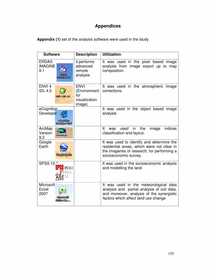
155
Appendices
Appendix (1) set of the analysis software were used in the study
Software Description Utilization
ERDAS IMAGINE 9.1
it performs advanced remote analysis
It was used in the pixel based image analysis from image export up to map composition.
ENVI 4 IDL 4.5
ENVI (Environment for visualization image)
It was used in the atmospheric Image corrections.
eCognition Developer
It was used in the object based image analysis
ArcMap Version 9.2
It was used in the image indices classification and layout.
Google Earth
It was used to identify and determine the residential areas, which were not clear in the imageries of research, for performing a socioeconomic survey.
SPSS 10.0
It was used in the socioeconomic analysis and modelling the land
Microsoft Excel 2007
It was used in the meteorological data analysis and partial analysis of soil data, and moreover, analysis of the synergistic factors which affect land use change
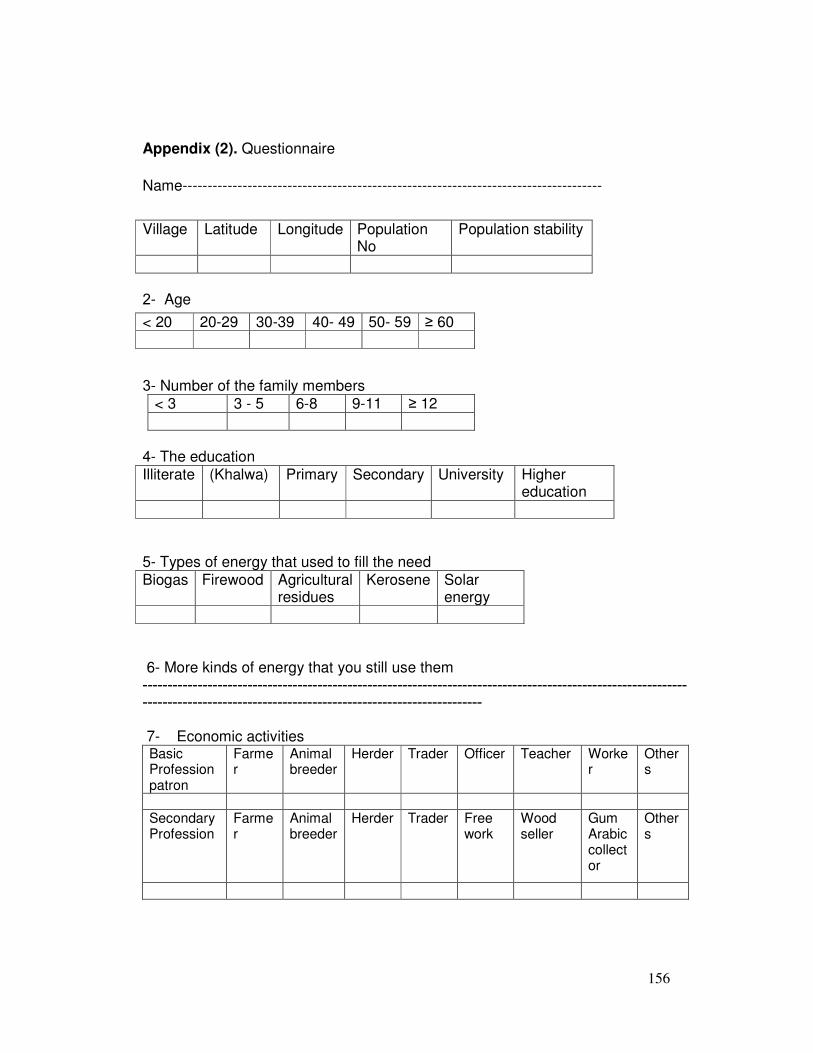
156
Appendix (2). Questionnaire Name------------------------------------------------------------------------------------
Village Latitude Longitude Population
No Population stability
2- Age
3- Number of the family members
≥ 12 9-11 6-8 3 - 5 < 3
4- The education
Higher education
University Secondary Primary (Khalwa) Illiterate
5- Types of energy that used to fill the need
Solar energy
Kerosene Agricultural residues
Firewood Biogas
6- More kinds of energy that you still use them
------------------------------------------------------------------------------------------------ -------------
-------------------------------------------------------------------- 7- Economic activities
Others
Worker
Teacher Officer Trader Herder Animal breeder
Farmer
Basic Profession patron
Others
Gum Arabic collector
Wood seller
Free work
Trader Herder Animal breeder
Farmer
Secondary Profession
< 20 20-29 30-39 40- 49 50- 59 ≥ 60
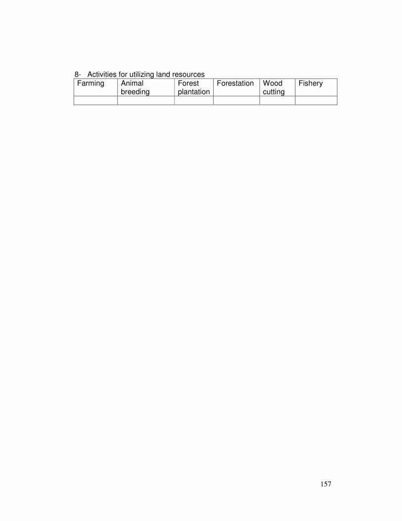
157
8- Activities for utilizing land resources
Fishery Wood cutting
Forestation Forest plantation
Animal breeding
Farming
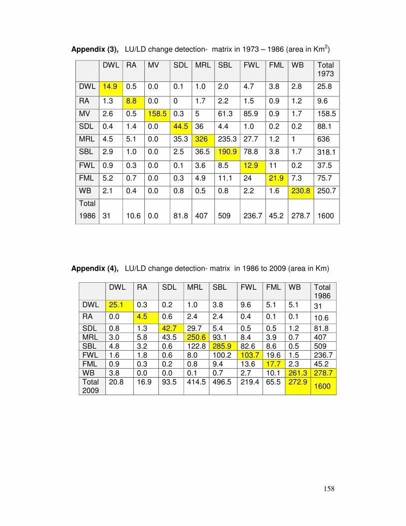
158
Appendix (3), LU/LD change detection- matrix in 1973 – 1986 (area in Km2)
Appendix (4), LU/LD change detection- matrix in 1986 to 2009 (area in Km)
DWL RA SDL MRL SBL FWL FML WB Total 1986
DWL 25.1 0.3 0.2 1.0 3.8 9.6 5.1 5.1 31 RA 0.0 4.5 0.6 2.4 2.4 0.4 0.1 0.1 10.6 SDL 0.8 1.3 42.7 29.7 5.4 0.5 0.5 1.2 81.8 MRL 3.0 5.8 43.5 250.6 93.1 8.4 3.9 0.7 407 SBL 4.8 3.2 0.6 122.8 285.9 82.6 8.6 0.5 509 FWL 1.6 1.8 0.6 8.0 100.2 103.7 19.6 1.5 236.7 FML 0.9 0.3 0.2 0.8 9.4 13.6 17.7 2.3 45.2 WB 3.8 0.0 0.0 0.1 0.7 2.7 10.1 261.3 278.7 Total 2009
20.8 16.9 93.5 414.5 496.5 219.4 65.5 272.9 1600
DWL RA MV SDL MRL SBL FWL FML WB Total 1973
DWL 14.9 0.5 0.0 0.1 1.0 2.0 4.7 3.8 2.8 25.8
RA 1.3 8.8 0.0 0 1.7 2.2 1.5 0.9 1.2 9.6
MV 2.6 0.5 158.5 0.3 5 61.3 85.9 0.9 1.7 158.5
SDL 0.4 1.4 0.0 44.5 36 4.4 1.0 0.2 0.2 88.1
MRL 4.5 5.1 0.0 35.3 326 235.3 27.7 1.2 1 636
SBL 2.9 1.0 0.0 2.5 36.5 190.9 78.8 3.8 1.7 318.1
FWL 0.9 0.3 0.0 0.1 3.6 8.5 12.9 11 0.2 37.5
FML 5.2 0.7 0.0 0.3 4.9 11.1 24 21.9 7.3 75.7
WB 2.1 0.4 0.0 0.8 0.5 0.8 2.2 1.6 230.8 250.7
Total
1986
31
10.6
0.0
81.8
407
509
236.7
45.2
278.7
1600
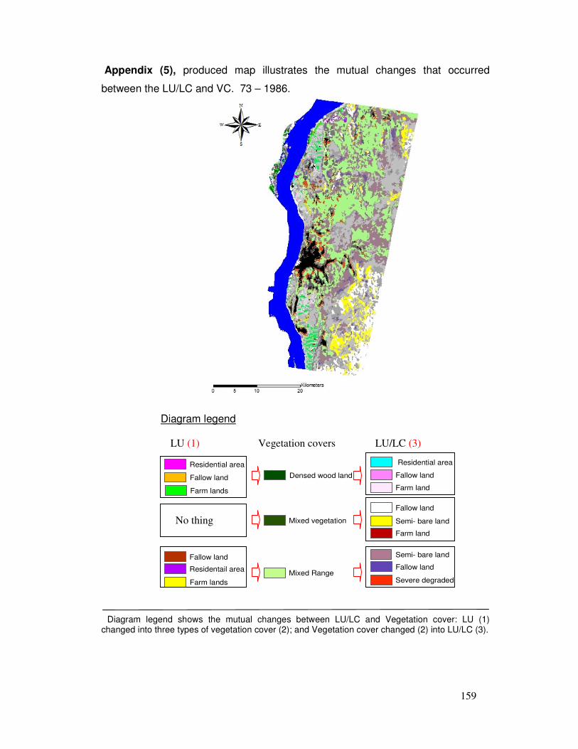
159
Densed wood land
Mixed vegetation
Mixed Range
Residential area
Fallow land
Farm land
Semi- bare land
Fallow land
Farm land
Severe degraded
Semi- bare land
Fallow land
Fallow land
Fallow land
Farm lands
Farm lands
Residential area
Residentail area
Appendix (5), produced map illustrates the mutual changes that occurred
between the LU/LC and VC. 73 – 1986.
Diagram legend
Diagram legend shows the mutual changes between LU/LC and Vegetation cover: LU (1) changed into three types of vegetation cover (2); and Vegetation cover changed (2) into LU/LC (3).
LU/LC (3) LU (1) Vegetation covers
No thing
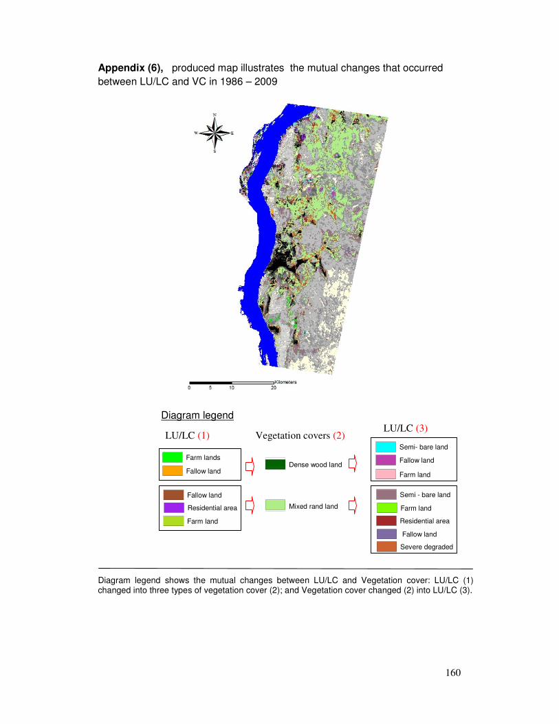
160
Appendix (6), produced map illustrates the mutual changes that occurred between LU/LC and VC in 1986 – 2009 Diagram legend Diagram legend shows the mutual changes between LU/LC and Vegetation cover: LU/LC (1) changed into three types of vegetation cover (2); and Vegetation cover changed (2) into LU/LC (3).
Dense wood land
Mixed rand landResidential area
Farm lands
Fallow land
Fallow land
Farm land
Severe degraded
Fallow land
Semi- bare land
Fallow land
Farm land
Residential area
Semi - bare land
Farm land
LU/LC (1) Vegetation covers (2) LU/LC (3)
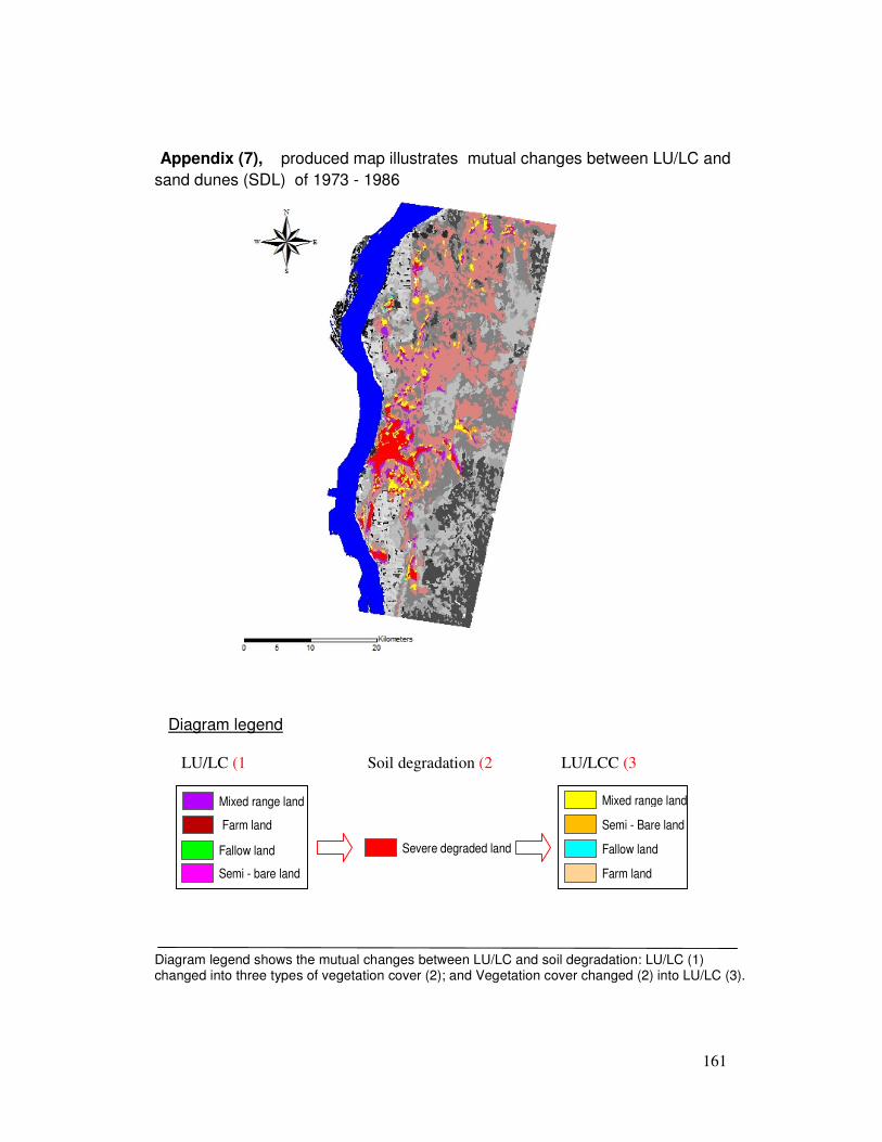
161
Severe degraded land
Mixed range land
Semi - Bare land
Fallow land
Farm land
Mixed range land
Semi - bare land
Fallow land
Farm land
Appendix (7), produced map illustrates mutual changes between LU/LC and sand dunes (SDL) of 1973 - 1986
Diagram legend
Diagram legend shows the mutual changes between LU/LC and soil degradation: LU/LC (1) changed into three types of vegetation cover (2); and Vegetation cover changed (2) into LU/LC (3).
LU/LCC (3 LU/LC (1 Soil degradation (2
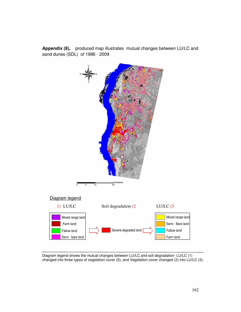
162
Severe degraded land
Mixed range land
Semi - Bare land
Fallow land
Farm land
Mixed range land
Semi - bare land
Fallow land
Farm land
Appendix (8), produced map illustrates mutual changes between LU/LC and sand dunes (SDL) of 1986 - 2009 Diagram legend
Diagram legend shows the mutual changes between LU/LC and soil degradation: LU/LC (1) changed into three types of vegetation cover (2); and Vegetation cover changed (2) into LU/LC (3).
1) LU/LC LU/LC (3 Soil degradation (2
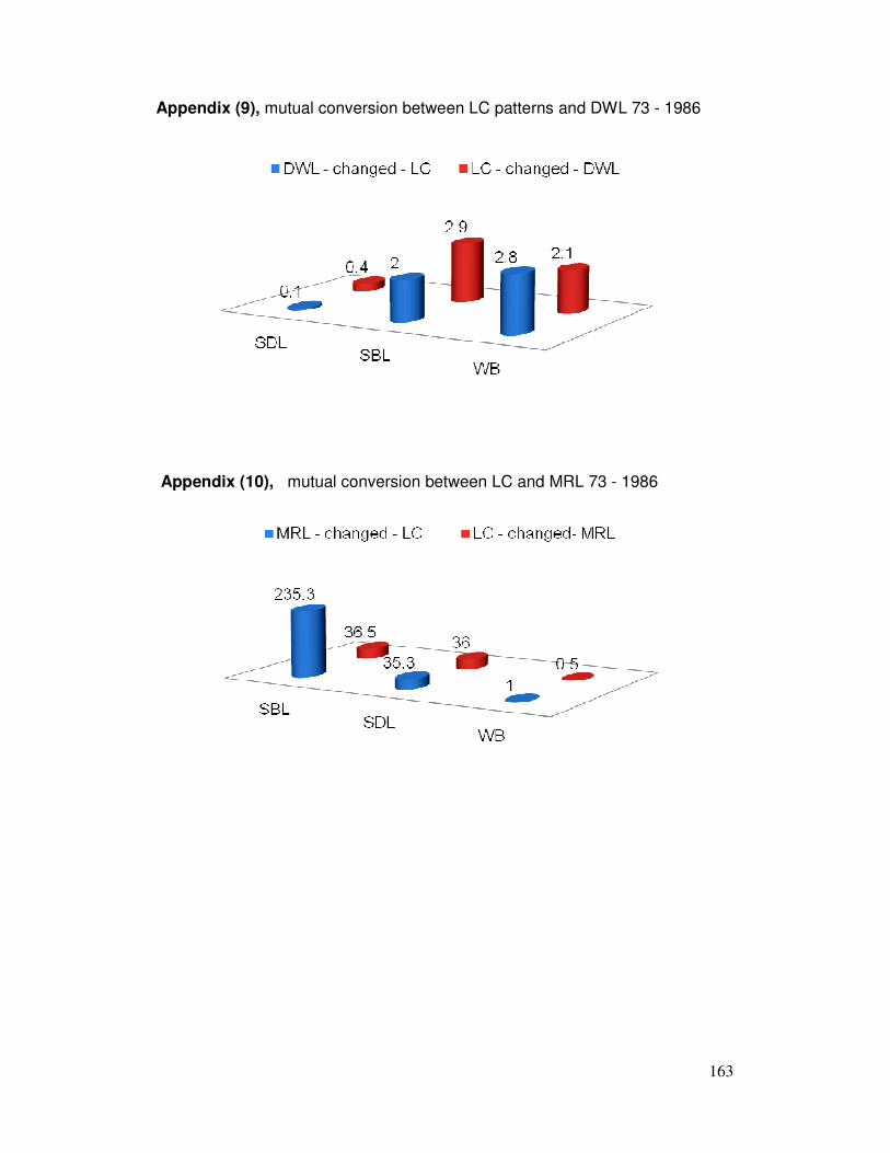
163
Appendix (9), mutual conversion between LC patterns and DWL 73 - 1986
Appendix (10), mutual conversion between LC and MRL 73 - 1986
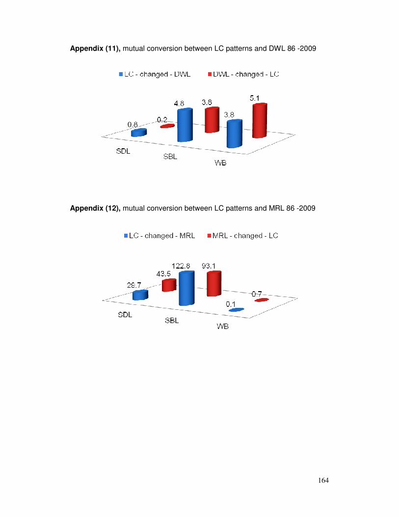
164
Appendix (11), mutual conversion between LC patterns and DWL 86 -2009
Appendix (12), mutual conversion between LC patterns and MRL 86 -2009
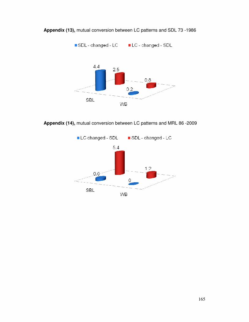
165
Appendix (13), mutual conversion between LC patterns and SDL 73 -1986
Appendix (14), mutual conversion between LC patterns and MRL 86 -2009
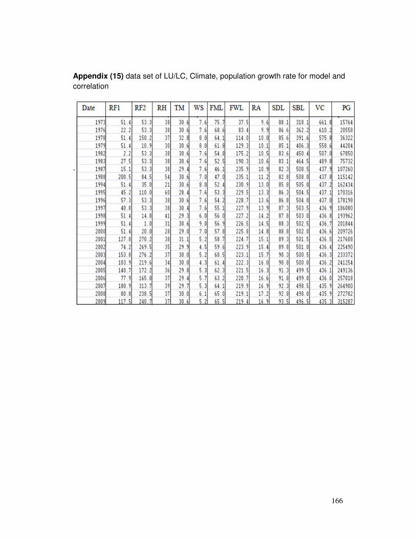
166
Appendix (15) data set of LU/LC, Climate, population growth rate for model and correlation
.
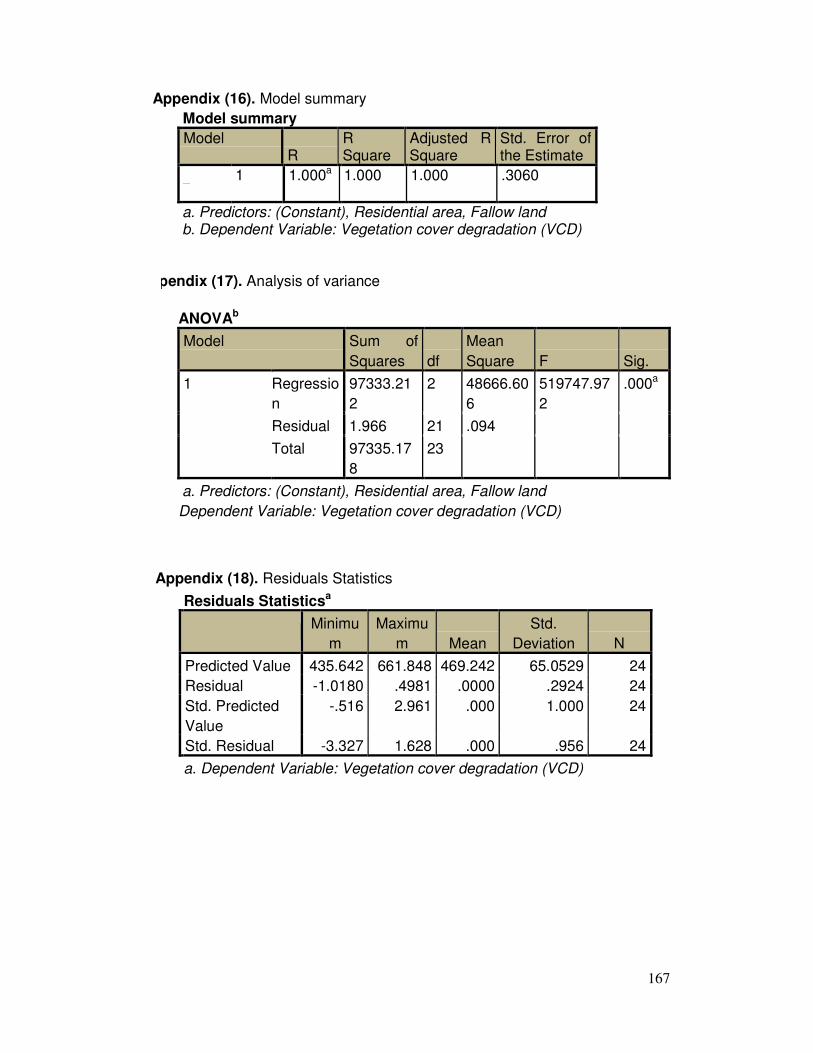
167
Appendix (16). Model summary
Appendix (18). Residuals Statistics
Residuals Statisticsa
Minimum
Maximum Mean
Std. Deviation N
Predicted Value 435.642 661.848 469.242 65.0529 24 Residual -1.0180 .4981 .0000 .2924 24 Std. Predicted Value
-.516 2.961 .000 1.000 24
Std. Residual -3.327 1.628 .000 .956 24
a. Dependent Variable: Vegetation cover degradation (VCD)
Model summary Model
R R Square
Adjusted R Square
Std. Error of the Estimate
dimension0
1 1.000a 1.000 1.000 .3060
a. Predictors: (Constant), Residential area, Fallow land b. Dependent Variable: Vegetation cover degradation (VCD)
Appendix (17). Analysis of variance
ANOVAb
Model Sum of Squares df
Mean Square F Sig.
1 Regression
97333.212
2 48666.606
519747.972
.000a
Residual 1.966 21 .094
Total 97335.178
23
a. Predictors: (Constant), Residential area, Fallow land
Dependent Variable: Vegetation cover degradation (VCD)
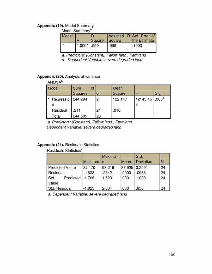
168
Appendix (19). Model Summary Model Summaryb Model
R R Square
Adjusted R Square
Std. Error of the Estimate
1 1.000a .999 .999 .1003
a. Predictors: (Constant), Fallow land , Farmland c. Dependent Variable: severe degraded land
Appendix (20). Analysis of variance
ANOVAb
Model Sum of Squares df
Mean Square F Sig.
1 Regression
244.294 2 122.147 12143.453
.000a
Residual .211 21 .010
Total 244.505 23
a. Predictors: (Constant), Fallow land , Farmland
Dependent Variable: severe degraded land
Appendix (21). Residuals Statistics
Residuals Statisticsa
Minimum
Maximum Mean
Std. Deviation N
Predicted Value 82.170 93.216 87.925 3.2591 24 Residual -.1628 .2842 .0000 .0958 24 Std. Predicted Value
-1.766 1.623 .000 1.000 24
Std. Residual -1.623 2.834 .000 .956 24
a. Dependent Variable: severe degraded land