Assessment of Models to Estimate Bus-Stop Level Transit

33

Assessment of Models to Estimate Bus-Stop Level Transit Ridership using Spatial Modeling Methods


Srinivas S. Pulugurtha, Ph.D., P.E., and Mahesh Agurla, M.S. The University of North Carolina at Charlotte

Abstract

The objective of this research is to develop and assess bus transit ridership models at a bus-stop level using two spatial modeling methods: spatial proximity method (SPM) and spatial weight method (SWM). Data for the Charlotte (North Carolina) area are used to illustrate 1) the working of the methods and 2) development and assessment of the models. Features available in Geographic Information System (GIS) software were explored to capture spatial attributes such as demographic, socio-economic, and land use characteristics around each selected bus stop. These, along with on-network characteristics surrounding the bus stop, were used as explanatory variables. Models were then developed, using the generalized estimating equations (GEE) framework, to estimate riders boarding (dependent variable) at the bus stop as a function of selected explanatory variables that are not correlated to each other. Results obtained indicate that Negative Binomial with log-link distribution better fits the data to estimate ridership at the bus-stop level (for both SPM and SWM) than when compared to linear, Poisson with log-link and Gamma with log-link dis-tributions. Although SPM models demonstrated distance decay behavior, statistical parameters indicate that SWM (based on functions 1/D, 1/D2, and 1/D3) does not yield better or more meaningful estimates than when compared to SPM using 0.25-mile buffer width data.

Journal of Public Transportation, Vol. 15, No. 1, 2012

34

IntroductionTransit systems support a broad range of goals that include air quality improve-ment, energy conservation, congestion reduction, provision of mobility to the disadvantaged, access to employment or attraction centers, the promotion of economic development, sustainability, and enhanced livability. Understanding the factors that influence transit ridership is very important to achieve these goals and increase transit market potential. The Bureau of Transportation Statistics (2010) reports that 6,922,000 people (~5% of the nation’s overall trips) used public trans-portation as their principal means of transportation to work each day during 2009.

Transit system managers and planners often rely on statistical models that are cost effective, developed in a reasonable amount of time using available data invento-ries, and provide a good understanding of the relationship between the dependent variable and explanatory variables. This research aims to develop statistical models to estimate riders boarding at a bus stop using spatial data and on-network char-acteristics around/near the bus stop. The data required to develop these models are typically available with most state Departments of Transportation and local agencies as well as in many open source data inventories.

The use of bus transit depends on accessibility to a bus stop. Accessibility could be defined in terms of walking time (say, 5, 10, 15, or 20 minutes from an origin to a bus stop) or walking distance (say, 0.25, 0.5, 0.75, or 1 mile from an origin to a bus stop). To better comprehend the substantial effect and area of influence of spatial attributes (includes explanatory variables such as demographic, socio-economic, land use, and on-network characteristics) on ridership (dependent variable), a spa-tial analysis needs to be conducted at several different buffer widths (say, 0.25, 0.5, 0.75, and 1 mile) to identify the ideal spatial proximity distance to extract data for modeling. The maximum buffer width for consideration depends on the accept-able maximum walking distance to access a bus stop (generally, 1 mile).

In general, the number of riders who use bus transit system decreases as the dis-tance from the bus stop increases. Integrating data pertaining to demographic, socio-economic, and land use characteristics from different buffer bandwidths (say, 0–0.25, 0.25–0.5, 0.5–0.75, and 0.75–1 mile) based on this distance decay effect, and using it to develop ridership models may yield better and accurate estimates.

The objective of this research is 1) to identify explanatory variables and distribu-tion functions and 2) to develop and assess ridership models at a bus-stop using two spatial modeling methods: spatial proximity method (SPM) and spatial weight

35


method (SWM). In this research, the number of riders boarding a bus transit system at a bus stop is considered as bus-stop ridership. Data for Charlotte (North Caro-lina) are used to illustrate 1) the working of the methods and 2) development and assessment of the models.

Literature Review As congestion in urban areas continues to worsen and highway solutions become less effective, many local governments and communities are turning their atten-tion to public transit. With the increasing pressure on transportation agencies to find ways to alleviate congestion and compete for limited federal funds to build premium transit systems that offer higher levels of service and a greater impact on ridership, there is an urgency to improve transit ridership analysis tools and models (Zhao et al. 2005).

Dajani and Sullivan (1976) conducted a study to develop a causal model for esti-mating public transit ridership using 1970 census data. Median income, percent central city workers, density, level of transit service, percent of African-American population, percent above age 65, and auto ownership were observed to be critical variables to estimate transit ridership. Nickesen et al. (1983) researched to develop a simple transit ridership estimation model for short-range transit planning. To ensure that the model can be applied easily and to produce accurate patronage estimates, the authors chose five component models (trip generation, trip distribu-tion, modal split, linear programming, and pivot point analysis) and applied them in a sequence.

Peng and Dueker (1995) studied relationships between inter-routes and the extent to which routes were independent, complementary, or competitive using spatial data integration of Portland (Oregon) data. The analyzed relationships were then used for route-level ridership modeling and to predict the ridership impacts of ser-vice changes, not only on the routes with service change but also on other related routes.

Kikuchi and Miljkovic (2001) developed transit ridership estimation models at a bus stop considering attributes pertaining to the bus stop (such as accessibility to the bus stop, demographic condition around the bus stop, conditions of the bus stop, and the transit service quality provided at the bus stop). T-BEST, a transit ridership estimation model, was developed by the Florida Department of Trans-portation (FDOT 2004; FDOT 2005) to estimate ridership by route, direction, and


36

time-of-day based on frequency, bus stop buffer characteristics, accessibility char-acteristics, and the effects of alternative routes and network design configurations.

Chu (2004) generated a transit ridership model at the bus stop for an average weekday boarding. Transit level-of-service (TLOS) based on transit availability and mobility and demographic characteristics, pedestrian environment, interactions with other modes, and competition from other bus stops were considered and found to play a significant role in predicting the ridership. Kimpel et al. (2007) examined the effects of overlapping walking service areas of bus stops on the demand for bus transit during the morning peak hour. Accessibility for each parcel to each bus stop was measured compared to other accessible bus stops in a GIS environment.

Sketch-level ridership forecast models for light or commuter rail (Lane et al. 2006) and heavy rail (Lane et al. 2009) for smaller- and medium-size cities were also developed in the past. The model developed was inexpensive compared to the traditional four-step modeling approach, since the data required to develop these models are readily available or can be easily obtained from Metropolitan Planning Organizations (MPOs) and/or the U.S. Census Bureau.

Transit ridership models were developed using a geographically weighted regres-sion (GWR) method exploring the spatial variability in the strength of the relation-ship between transit use and explanatory variables that included demographics, socio-economic, land use, transit supply and quality, and pedestrian environment characteristics (Chow et al. 2006; Chow et al. 2010). The coefficients in a GWR model are local and vary from one location to another location (unlike in ordinary least square regression models where coefficients interpret a global relationship between a dependent variable and explanatory variables). A comparison between the sub-regional GWR model (Chow et al. 2010) and the original regional GWR model (Chow et al. 2006) showed that the sub-regional GWR model performed better than the original regional GWR model in terms of model accuracy.

Cervero et al. (2010) recently developed a Direct Ridership Model (DRM) for Bus Rapid Transit (BRT) patronage in Southern California. The DRM was developed as a function of three key sets of variables related to bus stops or stations and their surroundings. The authors developed two linear regression models—ordinary least square (OLS) and hierarchical linear model (HLM). OLS was found to better fit the data than HLM. Results obtained from the study showed a strong influence of ser-vice frequency on BRT patronage in Los Angeles County.

37


Stover and Bae (2011) studied the impact of gasoline prices on transit ridership in Washington State by measuring the price elasticity of demand with respect to gasoline price. The results obtained indicate that transit ridership increased as gasoline prices increased during the study period.

Tang and Thakuriah (2011) examined if psychological effects of real-time transit information on commuters will lead to transit ridership gain. Findings from the study showed that the provision of real-time transit information might serve as an intervention to break current transit non-user travel habits and indeed increase the mode share of transit use. The study even suggested that real-time transit informa-tion would be more useful if it is combined with facilitating programs that enhance commuter opportunities to be exposed to such systems first.

Limitations of Past ResearchA review of past literature gives an understanding of the research methodologies that were adopted to estimate bus transit ridership at different levels (stop, route, city, and county). However, not much was documented based on spatial modeling, in particular, buffer or proximity analysis and spatially varying relationships. The effect of all the three characteristics (demographic and socio-economic, land use, and on-network) on bus transit ridership and the effect of correlation that could exist between these variables were not investigated widely in the past. Further, most of the transit ridership models developed in the past considered a linear rela-tionship between ridership and explanatory variables. While OLS, HLM or GWR-based OLS seem to be promising, non-linear or count models (such as generalized linear models) may be more appropriate for modeling in this case, as bus transit ridership are counts. This research attempts to address these above-mentioned limitations of past research (bus-stop non-linear ridership models exploring spa-tially varying relationships).

MethodologyA GIS-based methodology was adopted to extract spatial data and develop bus-stop ridership models using SPM and SWM. The methodology comprises the fol-lowing steps:

1. Identification of data elements for model development.2. Spatial analysis, data processing and spatial modeling methods.3. Statistical analysis and model development.


38

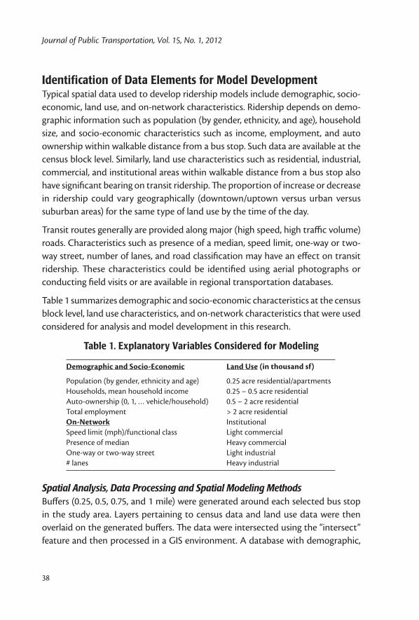
Identification of Data Elements for Model DevelopmentTypical spatial data used to develop ridership models include demographic, socio-economic, land use, and on-network characteristics. Ridership depends on demo-graphic information such as population (by gender, ethnicity, and age), household size, and socio-economic characteristics such as income, employment, and auto ownership within walkable distance from a bus stop. Such data are available at the census block level. Similarly, land use characteristics such as residential, industrial, commercial, and institutional areas within walkable distance from a bus stop also have significant bearing on transit ridership. The proportion of increase or decrease in ridership could vary geographically (downtown/uptown versus urban versus suburban areas) for the same type of land use by the time of the day.

Transit routes generally are provided along major (high speed, high traffic volume) roads. Characteristics such as presence of a median, speed limit, one-way or two-way street, number of lanes, and road classification may have an effect on transit ridership. These characteristics could be identified using aerial photographs or conducting field visits or are available in regional transportation databases.

Table 1 summarizes demographic and socio-economic characteristics at the census block level, land use characteristics, and on-network characteristics that were used considered for analysis and model development in this research.

Table 1. Explanatory Variables Considered for Modeling

Demographic and Socio-Economic Land Use (in thousand sf)

Population (by gender, ethnicity and age) 0.25 acre residential/apartmentsHouseholds, mean household income 0.25 – 0.5 acre residentialAuto-ownership (0, 1, … vehicle/household) 0.5 – 2 acre residentialTotal employment > 2 acre residentialOn-Network InstitutionalSpeed limit (mph)/functional class Light commercialPresence of median Heavy commercialOne-way or two-way street Light industrial# lanes Heavy industrial

Spatial Analysis, Data Processing and Spatial Modeling MethodsBuffers (0.25, 0.5, 0.75, and 1 mile) were generated around each selected bus stop in the study area. Layers pertaining to census data and land use data were then overlaid on the generated buffers. The data were intersected using the “intersect” feature and then processed in a GIS environment. A database with demographic,

39


socio-economic, and land use information in the vicinity of each bus stop, for each buffer width, was then generated. The spatial overlay and data processing approach is similar to the one used by Pulugurtha and Repaka (2009, 2011) to develop pedes-trian activity models for signalized intersections. On-network characteristics from aerial photographs, field visits, and the regional transportation network database were then added to these databases for each buffer width.

In this research, the working of two spatial modeling methods (SPM and SWM) to estimate ridership at the bus stop was evaluated.

Spatial Proximity Method (SPM) The first method, SPM, was used to evaluate the best proximity distance that has a strong influence on estimating ridership at a bus stop. Databases, as stated pre-viously, were generated to develop models to estimate bus-stop transit ridership for each buffer width (0.25, 0.5, 0.75, and 1 mile) discretely in this case. The model with buffer width data that has better goodness of fit statistics was selected as the best model. This buffer width was considered as the best ridership influence area (proximity distance) to estimate ridership for a bus stop.

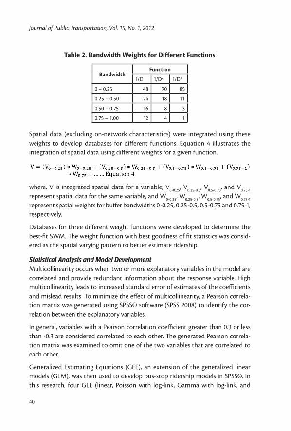
Spatial Weight Method (SWM)The second method, SWM, is a spatial modeling method that accounts for spa-tially-varying relationships. A weight pattern/procedure based on three spatially-decreasing functions (1/D, 1/D2, and 1/D3) were considered to evaluate and identify the function or weight combination that better estimates ridership at a bus stop. The data sets for 0.25-, 0.5-, 0.75-, and 1-mile buffer widths were used to create data for buffer bandwidths (0–0.25, 0.25–0.5, 0.5–0.75, and 0.75–1 mile). These bandwidths were given weights such that the total summation of weight is equal to 1. The calculation of weights for functions 1/D, 1/D2, and 1/D3 are mathematically shown in Equations 1 to 3.

where, D is the buffer width (0.25, 0.5, 0.75, or 1-mile).

Table 2 summarizes bandwidth weights for the three different functions consid-ered in this research.


40

Table 2. Bandwidth Weights for Different Functions

BandwidthFunction

1/D 1/D2 1/D3

0 – 0.25 48 70 85

0.25 – 0.50 24 18 11

0.50 – 0.75 16 8 3

0.75 – 1.00 12 4 1

Spatial data (excluding on-network characteristics) were integrated using these weights to develop databases for different functions. Equation 4 illustrates the integration of spatial data using different weights for a given function.

where, V is integrated spatial data for a variable; V0-0.25, V0.25-0.5, V0.5-0.75, and V0.75-1 represent spatial data for the same variable, and W0-0.25, W0.25-0.5, W0.5-0.75, and W0.75-1 represent spatial weights for buffer bandwidths 0-0.25, 0.25-0.5, 0.5-0.75 and 0.75-1, respectively.

Databases for three different weight functions were developed to determine the best-fit SWM. The weight function with best goodness of fit statistics was consid-ered as the spatial varying pattern to better estimate ridership.

Statistical Analysis and Model DevelopmentMulticollinearity occurs when two or more explanatory variables in the model are correlated and provide redundant information about the response variable. High multicollinearity leads to increased standard error of estimates of the coefficients and mislead results. To minimize the effect of multicollinearity, a Pearson correla-tion matrix was generated using SPSS© software (SPSS 2008) to identify the cor-relation between the explanatory variables.

In general, variables with a Pearson correlation coefficient greater than 0.3 or less than -0.3 are considered correlated to each other. The generated Pearson correla-tion matrix was examined to omit one of the two variables that are correlated to each other.

Generalized Estimating Equations (GEE), an extension of the generalized linear models (GLM), was then used to develop bus-stop ridership models in SPSS©. In this research, four GEE (linear, Poisson with log-link, Gamma with log-link, and

41


Negative Binomial with log-link) models were developed to evaluate the best distribution to estimate ridership at the bus stop. While linear distribution helps examine the presence of a strong linear relation between dependent and indepen-dent variables, the log-link (Gamma, Poisson, and Negative Binomial) distributions help examine the presence of a strong non-linear relation between dependent and independent variables.

In each case, a preliminary model was developed using an initial set of explanatory variables that are not correlated to other variables. Significance value was used to examine the strength of each variable. Those with significance value greater than 0.05 (at 95% confidence level) were eliminated one after another. The models were re-run in SPSS© environment until all the variables in the model had a significance value ≤ 0.05. The model when all variables had significance value ≤ 0.05 was con-sidered as the final model for the scenario and was used for assessment.

Quasi-likelihood criterion (QIC) and corrected quasi-likelihood under the indepen-dence model criterion (QICC) were used as statistics to assess the goodness of fit. In general, QIC and QICC should be low for a best fit model. The difference between QIC and QICC has to be reasonably low as well.

ResultsData for Charlotte (North Carolina) were gathered and used to illustrate the working of methods and development and assessment of models. The bus transit system in the region is operated and maintained by Charlotte Area Transit System (CATS). It serves over 70 routes (with 3,600+ bus stops), of which 56 are local routes and 19 are express routes. The average daily ridership during 2010 was more than 66,000 passengers.

Census estimates with demographic and socio-economic characteristics were obtained from the U.S. Census Bureau website. Land-use data and on-network characteristics were obtained from the City of Charlotte Department of Transpor-tation (CDOT). Bus-stop ridership (boarding only) data were obtained from CATS. All data considered in this research are for 2008.

The bus-stop level ridership data from CATS showed that the number of passen-gers boarding bus transit system was collected for at least one day at over 2,900 bus-stops during 2008. These data were processed to compute average daily rider-ship for each of these bus stops.


42

Of the bus stops for which ridership data were available, 2,857 bus stops were selected to develop ridership models. The average daily ridership for the selected bus stops is ~23. Of the 2,857 selected bus stops, 488 bus stops were observed to have ridership number greater than the average value.

As explained previously, explanatory variables that are not correlated to other variables were selected to minimize redundant explanatory variables and standard errors in the models. This was done separately for databases of each individual buffer width (0.25, 0.5, 0.75, and 1 mile) as well as the integrated databases for different weight functions.

Selection of Distribution Function that Better Fits the DataModels based on different probability distributions were developed, as it is critical to understand the probability distribution that better fits the ridership data. Four GEE models based on different probability distributions (linear, Poisson with log-link, Gamma with log-link, and Negative Binomial with log-link) were developed using data for each buffer width (0.25, 0.5, 075, and 1 mile). Overall, 16 models were developed based on SPM to evaluate and select the best proximity distance to capture spatial data.

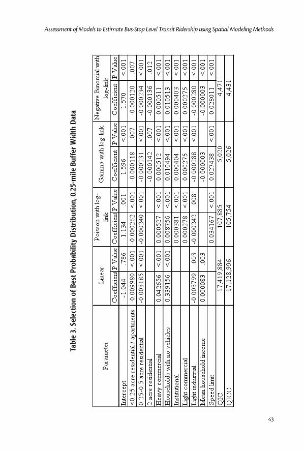
As an example, Table 3 summarizes results obtained for models based on the four probability distributions using 0.25-mile buffer width data. The information pre-sented in the table can be used to estimate ridership at a bus stop. While substitut-ing data (selected land-use areas, the number of households with no vehicles, mean household income, and speed limit along the corridor) gives a ridership estimate directly in the case of a model based on linear probability distribution, it gives a natural logarithm of ridership in the case of the other three log-link probability dis-tributions. QIC and QICC were compared to identify the distribution that best fits the data for each buffer width. Results obtained show that Negative Binomial with log-link with lowest QIC and QICC (difference between QIC and QICC reasonably low) best fits the data for each selected buffer width.

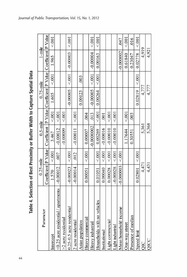
Selection of Ideal Proximity Distance to Extract Spatial DataTable 4 summarizes parameters of four (Negative Binomial with log-link) models developed using data for different buffer widths (0.25, 0.5, 0.75, and 1 mile). The model developed using the 0.25 buffer width data has the lowest QIC and QICC (difference between QIC and QICC reasonably low) when compared to models developed using data for other buffer widths (0.5, 0.75, and 1,mile). For the data used in this research, this is the best SPM, and 0.25-mile is the best proximity dis-tance that estimates the average daily ridership at the bus-stop.

43


Tabl

e 3.

Sel

ecti

on o

f Bes

t Pro

babi

lity

Dis

trib

utio

n, 0

.25-

mile

Buf

fer

Wid

th D

ata


44

Tabl

e 4.

Sel

ecti

on o

f Bes

t Pro

xim

ity

or B

uffe

r W

idth

to C

aptu

re S

pati

al D

ata

45


The strength of explanatory variables, in general, decreased while goodness-of-fit statistics increased as the distance from the bus stop increased. In other words, results from SPM for different buffer widths tend to show distance decay behavior. This probably indicates that better and more accurate estimates may be obtained by developing models using data integrated from different buffer widths.

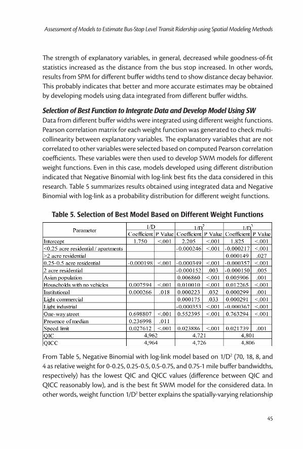
Selection of Best Function to Integrate Data and Develop Model Using SWData from different buffer widths were integrated using different weight functions. Pearson correlation matrix for each weight function was generated to check multi-collinearity between explanatory variables. The explanatory variables that are not correlated to other variables were selected based on computed Pearson correlation coefficients. These variables were then used to develop SWM models for different weight functions. Even in this case, models developed using different distribution indicated that Negative Binomial with log-link best fits the data considered in this research. Table 5 summarizes results obtained using integrated data and Negative Binomial with log-link as a probability distribution for different weight functions.

Table 5. Selection of Best Model Based on Different Weight Functions

From Table 5, Negative Binomial with log-link model based on 1/D2 (70, 18, 8, and 4 as relative weight for 0-0.25, 0.25-0.5, 0.5-0.75, and 0.75-1 mile buffer bandwidths, respectively) has the lowest QIC and QICC values (difference between QIC and QICC reasonably low), and is the best fit SWM model for the considered data. In other words, weight function 1/D2 better explains the spatially-varying relationship


46

between ridership and independent variables than the other two weight functions considered in this research.

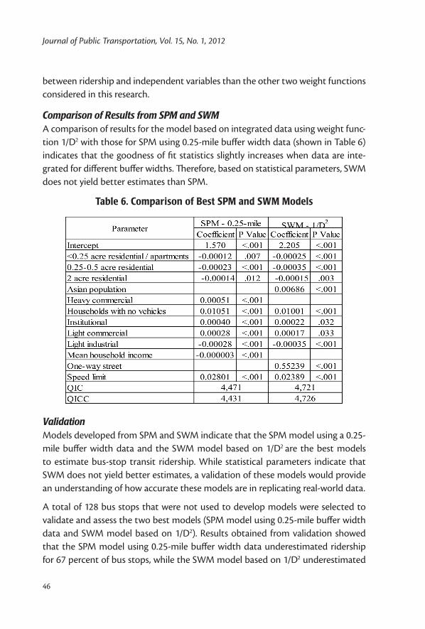
Comparison of Results from SPM and SWMA comparison of results for the model based on integrated data using weight func-tion 1/D2 with those for SPM using 0.25-mile buffer width data (shown in Table 6) indicates that the goodness of fit statistics slightly increases when data are inte-grated for different buffer widths. Therefore, based on statistical parameters, SWM does not yield better estimates than SPM.

Table 6. Comparison of Best SPM and SWM Models

ValidationModels developed from SPM and SWM indicate that the SPM model using a 0.25-mile buffer width data and the SWM model based on 1/D2 are the best models to estimate bus-stop transit ridership. While statistical parameters indicate that SWM does not yield better estimates, a validation of these models would provide an understanding of how accurate these models are in replicating real-world data.

A total of 128 bus stops that were not used to develop models were selected to validate and assess the two best models (SPM model using 0.25-mile buffer width data and SWM model based on 1/D2). Results obtained from validation showed that the SPM model using 0.25-mile buffer width data underestimated ridership for 67 percent of bus stops, while the SWM model based on 1/D2 underestimated

47


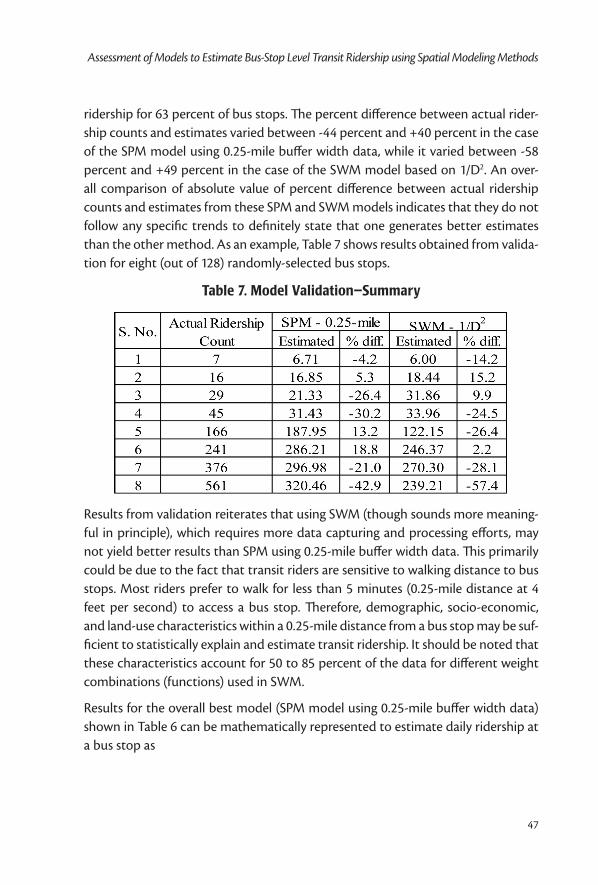
ridership for 63 percent of bus stops. The percent difference between actual rider-ship counts and estimates varied between -44 percent and +40 percent in the case of the SPM model using 0.25-mile buffer width data, while it varied between -58 percent and +49 percent in the case of the SWM model based on 1/D2. An over-all comparison of absolute value of percent difference between actual ridership counts and estimates from these SPM and SWM models indicates that they do not follow any specific trends to definitely state that one generates better estimates than the other method. As an example, Table 7 shows results obtained from valida-tion for eight (out of 128) randomly-selected bus stops.

Table 7. Model Validation–Summary

Results from validation reiterates that using SWM (though sounds more meaning-ful in principle), which requires more data capturing and processing efforts, may not yield better results than SPM using 0.25-mile buffer width data. This primarily could be due to the fact that transit riders are sensitive to walking distance to bus stops. Most riders prefer to walk for less than 5 minutes (0.25-mile distance at 4 feet per second) to access a bus stop. Therefore, demographic, socio-economic, and land-use characteristics within a 0.25-mile distance from a bus stop may be suf-ficient to statistically explain and estimate transit ridership. It should be noted that these characteristics account for 50 to 85 percent of the data for different weight combinations (functions) used in SWM.

Results for the overall best model (SPM model using 0.25-mile buffer width data) shown in Table 6 can be mathematically represented to estimate daily ridership at a bus stop as


48

(5)

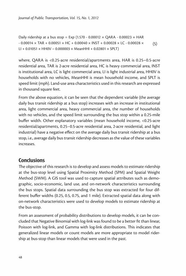
where, QARA is <0.25-acre residential/apartments area, HAR is 0.25–0.5-acre residential area, TAR is 2-acre residential area, HC is heavy commercial area, INST is institutional area, LC is light commercial area, LI is light industrial area, HH0V is households with no vehicles, MeanHHI is mean household income, and SPLT is speed limit (mph). Land-use area characteristics used in this research are expressed in thousand square feet.

From the above equation, it can be seen that the dependent variable (the average daily bus transit ridership at a bus stop) increases with an increase in institutional area, light commercial area, heavy commercial area, the number of households with no vehicles, and the speed limit surrounding the bus stop within a 0.25-mile buffer width. Other explanatory variables (mean household income, <0.25-acre residential/apartments, 0.25–0.5-acre residential area, 2-acre residential, and light industrial) have a negative effect on the average daily bus transit ridership at a bus stop, i.e., average daily bus transit ridership decreases as the value of these variables increases.

ConclusionsThe objective of this research is to develop and assess models to estimate ridership at the bus-stop level using Spatial Proximity Method (SPM) and Spatial Weight Method (SWM). A GIS tool was used to capture spatial attributes such as demo-graphic, socio-economic, land use, and on-network characteristics surrounding the bus stops. Spatial data surrounding the bus stop was extracted for four dif-ferent buffer widths (0.25, 0.5, 0.75, and 1 mile). Extracted spatial data along with on-network characteristics were used to develop models to estimate ridership at the bus-stop.

From an assessment of probability distributions to develop models, it can be con-cluded that Negative Binomial with log-link was found to be a better fit than linear, Poisson with log-link, and Gamma with log-link distributions. This indicates that generalized linear models or count models are more appropriate to model rider-ship at bus-stop than linear models that were used in the past.

Daily ridership at a bus stop = Exp (1.570 - 0.00012 × QARA - 0.00023 × HAR - 0.00014 × TAR + 0.00051 × HC + 0.00040 × INST + 0.00028 × LC - 0.00028 × LI + 0.01051 × HH0V – 0.000003 × MeanHHI + 0.02801 × SPLT)

49


From an assessment of models based on data for different widths, it can be concluded that the model developed using a 0.25-mile buffer width has better goodness-of-fit values than 0.5-, 0.75-, and 1-mile buffer widths. It is, therefore, rec-ommended as the best proximity distance to capture spatial data and estimate rid-ership at the bus-stop. In general, SPM models exhibited distance decay behavior.

The SWM model with Negative Binomial distribution using weights as a function of 1/D2 (relative weights of 70, 18, 8, 4 for buffer bandwidths 0–0.25, 0.25–0.5, 0.5–0.75, and 0.75–1 mile, respectively) was found to be the best model than when compared to function 1/D and 1/D3 to estimate ridership at the bus stop.

A comparison of results (model parameters) obtained from the two spatial model-ing methods (SPM and SWM) suggests that SWM models do not yield statistically different outputs than the SPM model using 0.25-mile buffer width data. Results obtained from validation further support that using SWM may not yield better results than SPM using 0.25-mile buffer width data. Therefore, demographic, socio-economic, and land use characteristics within a 0.25-mile distance from a transit stop are sufficient to statistically explain and estimate bus stop transit ridership. This also indicates that riders are sensitive to walking distance to access a bus stop. More than 50 percent of riders prefer to walk ≤ 0.25 miles to access bus stops.

Models developed from the statistical analysis indicate that ridership will be high in areas with households with no vehicles, institutions, and commercial establish-ments, whereas ridership will be low in areas with residences and high mean house-hold income. Outcomes from this research help the decision makers and planners to better estimate bus transit ridership and identify public transit infrastructure that support sustainability as well as livability and a better quality of life for next generations.

In this research, the effect of overlapping buffer areas and temporal variation was not considered. Further research on distance decay measure is necessary to determine the effect of overlapping buffer areas to better estimate ridership at the bus-stop level. The function and how sensitive riders are to walking distance varies with the type of public transportation system (bus transit vs. monorail vs. light rail transit vs. commuter rail). It also may vary based on the geographic location of bus stops (downtown/uptown versus urban versus suburban areas) and time of the day. Models for different modes of public transportation by geographic location and time of the day, therefore, need to be developed.


50

Some of the most influential explanatory variables on bus transit ridership (such as the effect of increases in gasoline price, service quality or level of service, provision of real-time transit information, trip cost, and patron safety) were not considered due to data availability constraints. Examining the effect of these variables in addi-tion to those considered in this research and developing transit ridership models needs further investigation.

References

Bureau of Transportation Statistics. 2010. National Transportation Statistics. Principal means of transportation to work. Available at: http://www.bts.gov/publications/national_transportation_statistics/2010/html/table_01_38.html (accessed June 8, 2011).

Cervero, R., J. Murakami, and M. Miller. 2010. Direct ridership model of bus rapid transit in Los Angeles County, California. Transportation Research Record 2145: 1-7.

Chow, L. F., F. Zhao, X. Liu, M. T. Li, and I. Ubaka. 2006. Transit ridership model based on Geographically Weighted Regression. Transportation Research Record 1972: 105-114.

Chow, L. F., F. Zhao, H. Chi, and Z. Chen. 2010. Subregional transit ridership models based on Geographically Weighted Regression. Transportation Research Board 89th Annual Meeting Compendium of Papers DVD, Washington, D.C.

Chu, X. 2004. Ridership models at the stop level. Report No. BC137-31, Prepared by National Center for Transit Research for Florida Department of Transporta-tion.

Dajani, J. S., and D. A. Sullivan. 1976. A causal model for estimating public transit ridership using census data. High Speed Ground Transportation Journal 10(1): 47-57.

Florida Department of Transportation (FDOT). 2004. Enhancement and refine-ment of the integrated transit and demand and supply model, T-BEST Arc Version 1.1, Users Guide. Public Transit Office, FDOT, Tallahassee, FL.

FDOT. 2005. Enhancement and refinement of the integrated transit and demand and supply model, T-BEST Arc Version 2.1, Users Guide. Public Transit Office, FDOT, Tallahassee, FL.

51


Kikuchi, S., and D. Miljkovic. 2001. Use of fuzzy inference for modeling prediction of transit ridership at individual stops. Transportation Research Record 1774: 25-35.

Kimpel, T. J., K. J. Dueker, and A. M. El-Geneidy. 2007. Using GIS to measure the effect of overlapping service areas on passenger boardings at bus stops. URISA Journal 19(1): 5-11.

Lane, C., M. DiCarlantonio, and L. Usvyat. 2006. Sketch model to forecast com-muter and light rail ridership. Transportation Research Record 1986: 198-210.

Lane, C., M. DiCarlantonio, L. Meckel, and L. Usvyat. 2009. Sketch model to forecast heavy rail ridership. Transportation Research Board 88th Annual Meeting Com-pendium of Papers DVD, Washington, D.C.

Nickesen, A. H., A. H. Meyburg, and M. A. Turnquist. 1983. Ridership estimation for short-range transit planning. Transportation Research Part B: Methodological 17B(3): 233-244.

Peng, Z., and K. J. Dueker. 1995. Spatial data integration in route-level transit demand modeling. Journal of the Urban and Regional Information Systems Association 7(1): 6-37.

Pulugurtha, S. S., and S. R. Repaka. 2009. An assessment of models to measure pedestrian activity at signalized intersections. Transportation Research Record 2073: 39-48.

Pulugurtha, S. S., and S. R. Repaka. 2011. An assessment of models to estimate pedestrian demand based on the level of activity. Journal of Advanced Trans-portation (in press).

SPSS Inc. 2008. SPSS® 16.0 Brief Guide, Copyright © 2008 by SPSS Inc., 233 South Wacker Drive, 11th Floor, Chicago, IL.

Stover, V. W., and C. H. C. Bae. 2011. The impact of gasoline prices on transit rider-ship in Washington State. Transportation Research Board 90th Annual Meet-ing Compendium of Papers DVD, Washington, D.C.

Tang, L., and P. Thakuriah. 2011. Will psychological effects of real-time transit infor-mation systems lead to ridership gain? Transportation Research Board 90th Annual Meeting, Compendium of Papers DVD, Washington, DC.

Zhao, F., L. F. Chow, X. Liu, and M. T. Li. 2005. A Transit ridership model based on Geographically Weighted Regression and service quality variables. Available


52

at: http://lctr.eng.fiu.edu/re-project-link/finalDO97591_BW.pdf (accessed June 8, 2011).

Acknowledgments

The authors acknowledge the staff of Charlotte Area Transit System (CATS) and the City of Charlotte Department of Transportation (CDOT) for their help with data.

About the Authors

Srinivas S. Pulugurtha ([email protected]) is currently working as an Associ-ate Professor of Civil and Environmental Engineering and an Assistant Director of the Center for Transportation Policy Studies at The University of North Carolina at Charlotte. His areas of interest include traffic safety, GIS applications, transportation planning/modeling, traffic simulation, and development of decision support tools.

Mahesh Agurla ([email protected]) is a graduate student in Transportation Engi-neering at The University of North Carolina at Charlotte.

Documents

Assessment of Models to Estimate Bus-Stop Level Transit