Embed Size (px)
Citation preview

TRITA-LWR Degree Project 13:40 ISSN 1651-064X LWR-EX-13-40
ASSESSMENT OF NUTRIENT LOADING IN LAKE RINGSJÖN FROM THE
CATCHMENT OF HÖRBYÅN CREEK IN SOUTHERN SWEDEN
Durgesh Kumar Singh
October 2013

Durgesh Kumar Singh TRITA LWR Degree Project 13:40
ii
© Durgesh Kumar Singh 2013 Environmental Engineering and Sustainable Infrastructure (EESI) Done in association with the River Engineering Research group Department of Land and Water Resources Engineering Royal Institute of Technology (KTH) SE-100 44 STOCKHOLM, Sweden Reference should be written as: Singh, D K (2013) “Assessment of nutrient loading in lake Ringsjön from the catchment of Hörbyån Creek in Southern Sweden” TRITA-LWR Degree Project 13:40

Assessment of nutrient loading in lake Ringsjön from catchment of Hörbyån Creek
iii
SUMMARY IN ENGLISH
Lake Ringsjön located in south of Sweden in Skåne County, has been subject of eutrophication since 1950s and received several restoration efforts. Latest restoration effort “Project Ringsjön” was proposed in 2003 to improve lake condition against eutrophication by reducing nutrient concentration. This study was done to assess the nutrient loading into the lake from the catchment of Hörbyån creek, which is discharging into the lake from southeast. Study addresses the nutrient loading conditions from Hörbyån creek before and after the implementation of “Project Ringsjön” in 1998 and 2010 respectively. Thus a water quality analysis was performed to observe the changes in total nitrogen and phosphorus concentration in Hörbyån creek between these years. Effort was also made to investigate nutrients contribution of different watersheds in the catchment. This study also addresses the effect of seasonal variability and land use on nutrient loading. In order to achieve objectives, annual and monthly water quality modelling was performed on the river. HEC-RAS software was used to simulate water quality variables such as nitrates, nitrite, ammonium, organic nitrogen, inorganic phosphorus and orthophosphate in the water carried by creek from catchment into the lake. This module of HEC-RAS (water quality simulation) was performed doing steady flow analysis, temperature analysis followed by water quality analysis. Study required data for river schematic, river geometry, flow discharge, boundary condition, and information regarding water quality variable. Information for land use condition and seasonal variability, such as information for agriculture, forest, urban land area, precipitation, temperature etc. were also analyzed for different watersheds to observe their impact on nutrient loading. Results from steady flow analysis indicated decrease in flow discharge by 39-40% from 1998 to 2010, probably due to reduction in precipitation and runoff in 2010 as compare to 1998. Results from water quality analysis indicated increase in average annual nitrogen concentration from 4.18 mg/l to 4.56 mg/l and reduction in average annual phosphorus concentration from 0.165 mg/l to 0.083 mg/l in the water discharging into the lake from catchment. The watershed containing mostly agriculture area was observed to have maximum contribution in nutrient loading, probably because of high fertilizer leakage with run off. It was also observed that maximum of nutrient loading is taking place from November to March; probably due to high runoff generated from precipitation and snow melting that carried additional nutrients to the water bodies. Results also indicated that the studied catchment area was contributing high nutrient concentration for eutrophication in both years; however, there was small decrease in total phosphorus concentration in 2010 from 1998.

Durgesh Kumar Singh TRITA LWR Degree Project 13:40
iv

Assessment of nutrient loading in lake Ringsjön from catchment of Hörbyån Creek
v
SUMMARY IN SWEDISH
Ringsjön, belägen i södra Sverige, har varit övergödd sedan 1950-talet. Flera försök att förbättra vattenkvaliteten har gjorts. Det senaste försöket, "Projekt Ringsjön", påbörjades 2003 för att minska koncentrationen av näringsämnen. Denna studie gjordes för att utvärdera den näringsbelastning tillstånd före och efter genomförandet av "Projekt Ringsjön" (1998 respektive 2010) från ett av sina avrinningsområden, Hörbyån, belägen sydöst om sjön. Således gjorde en vattenkvalitetsanalys för att observera förändringar i kväve- och fosforkoncentration 1998-2010. Försöken gjordes också för att analysera bidraget från de olika avrinningsområdena i avrinningsområdet i näringsbelastning och för att undersöka effekten av säsongsmässiga variationer. En vattenkvalitetsmodellering utfördes med hjälp av HEC-RAS, det vill säga programvara för att simulera vattenkvalitetsvariabler såsom nitrater, nitrit, ammonium, organiskt kväve, oorganisk fosfor och ortofosfat i floden som rinner från sjön. Denna modul av HEC-RAS utfördes under stadigt flöde av analys, temperatur analys följt av vattenkvalitet analys i slutet. Studien krävdes data för floden schematisk, flod geometri, flöde urladdning, randvillkor, och information om vattenkvalitetsvariabel. Markanvändning, skick och säsongsbetonade variationer, såsom jordbruk, skog, tätort, nederbörd, temperatur, etc. analyserades också för olika vattendelare område att observera deras inverkan på näringsbelastningen. Resultat från den stabila flödesanalysen visade på en minskning i flöde med 39-40 % från 1998 till 2010 förmodligen på grund av minskad nederbörd och avrinning under 2010, jämfört med 1998. Resultat från vattenkvalitetsanalysen visade på en ökning av den genomsnittliga kvävekoncentrationen från 4,18 mg/l till 4,56 mg/l, medan minskningen i genomsnittliga fosforkoncentrationen från 0,165 mg/l till 0,083 mg/l. Waters Hed som bestående av jordbruksområden tycks ha det maximala bidraget i näringsbelastning, troligen på grund av läckage av gödsel (innehållande kväve och fosfor). Det observerades också att näringsbelastningen som högst mellan november och mars, vilket skulle kunna bero på fortsätt snö och snösmältning, vilket transporterar näringsämnen till vattendragen. Resultaten har visat att det studerade avrinningsområdet bidrar till den höga koncentrationen av näringsämnen för övergödning, även om det är liten minskning i den totala fosforbelastningen 1998-2010.

Durgesh Kumar Singh TRITA LWR Degree Project 13:40
vi

Assessment of nutrient loading in lake Ringsjön from catchment of Hörbyån Creek
vii
ACKNOWLEDGEMENT I would like to express special thanks to my supervisor Andrea Bottacin Busolin, Assistant Professor in Department of Land and Water Resource Engineering, Royal Institute of Technology (KTH), for providing me all necessary guidance and help, along with a great learning opportunity during the period of my Master thesis. I would also like to express my sincere thanks to my friends, Harpa Dögg Magnúsdóttir and Caroline Le Lann Roos, for their contribution in preparing Swedish summary of my thesis report. I would also like to pay my gratitude to my parents and other members of my family, Nandita Singh, Harpa Dögg Magnúsdóttir, and other friends who have always been supporting during the entire time I needed them. In the end, I would like to extend my sincere thanks to European commission for providing financial assistant for my Master study.

Durgesh Kumar Singh TRITA LWR Degree Project 13:40
viii

Assessment of nutrient loading in lake Ringsjön from catchment of Hörbyån Creek
ix
TABLE OF CONTENT
Summary in English iii Summary in Swedish v Acknowledgement vii Table of Content ix Abstract 1 Introduction 1 Background 3 Significance of study 4 Objective 4
Literature review 4 Eutrophication and nutrients 4 Source contributing nutrient 6 Nutrients Leakage 6 Various factors affecting nutrient leakage 7
Model HEC-‐RAS 8 HEC RAS overview 8 Theoretical basis for steady flow analysis 10 Theoretical basis of water quality analysis 12 Temperature Dependence of Rate Reactions 13 Algae 13 Nitrogen Parameters 15 Phosphorus parameters 17 Carbonaceous Biological Oxygen Demand (CBOD) 17 Dissolved Oxygen (DOX) 17
Study area 18 Lake Ringsjön 19 Hörbyån Creek 19 Climate 19 Population 20 Watershed division and land use 21
Methodology 22 Research framework 22 Methods and material 23 Preparation for model setup 23 Database and data retrieval 23 Model setup 25 Lumped estimate of nutrient concentrations 29
Results 29 Discussion 37 Conclusion 40 References 41 Other References 42 Appendix – Supplementary information 44


Assessment of nutrient loading in lake Ringsjön from catchment of Hörbyån Creek
1
ABSTRACT
Lake Ringsjön, located in south of Sweden, has been subject of eutrophication since 1950s and received several restoration efforts. Latest restoration effort, “Project Ringsjön”, was proposed in 2003 to improve lake condition against eutrophication by reducing nutrient concentration. This study was done to assess the nutrient loading into the lake from the catchment of Hörbyån Creek, which is discharging into the lake from southeast. Study addresses the nutrient loading conditions from Hörbyån Creek before and after the implementation of “Project Ringsjön” in 1998 and 2010 respectively. Thus a water quality analysis was performed to observe the changes in total nitrogen and total phosphorus concentration in Hörbyån Creek between these years. Effort was also made to investigate nutrients contribution of different watersheds in the catchment. This study also addresses the effect of seasonal variability and land use on nutrient loading. In order to achieve objectives, annual and monthly water quality modelling was performed on the river. HEC-RAS software was used to simulate water quality variables loading from catchment into the lake, such as nitrates, nitrite, ammonium, organic nitrogen, inorganic phosphorus and orthophosphate. Results indicated increase in average annual total nitrogen concentration from 4.18 mg/l to 4.56 mg/l and reduction in average annual total phosphorus concentration from 0.165 mg/l to 0.083 mg/l in the water discharging into the lake from catchment. The watershed occupying mostly agriculture area was observed to have maximum nutrients contribution, which might be due to high fertilizer leakage. It was also observed that maximum nutrient loading was taking place in November and March; probably due to high runoff generated from precipitation and snow melting that carried additional nutrients to the water bodies. Results also indicated that the studied catchment area was contributing high nutrient concentration for eutrophication in both years; however, there was small decrease in total phosphorus concentration in 2010 compare to 1998.
Key words: Eutrophication, Nutrient loading, HEC-RAS and Water Quality Analysis.
INTRODUCTION
Water is essential component for proper functioning of earth ecosystem. All living bodies on earth are depending upon water for their life. Plants use water during photosynthesis and animals (including humans) use water directly or indirectly to sustain their multiple need of life. However continues exploitation of resources and increased anthropogenic activities on natural resources has tremendously amplified the pressure on availability of quality water, which further again cause the scarcity of quality water for proper functioning of ecosystem (Afeta, 2006). “Although we as humans recognize this fact, we disregard it by polluting our rivers, lakes, and oceans. Subsequently, we are slowly but surely harming our planet to the point where organisms are dying at an alarming rate. In addition to innocent organisms dying off, our drinking water has become greatly affected, as is our ability to use water for recreational purposes. In order to compact water pollution, we must understand the problems and become part of the solution” (Afeta, 2006). Overconsumption of water by industries and farmers has been affecting ecosystems and environment in many water basins that in turn has been threatening reliable water supply. Situation is further getting worse with the population growth, urbanization, intensifying farming, overuse of fertilizer and pesticide (Lambooy, 2011). Water contamination can occur either by point source, such as municipal sewage and industrial discharge

Durgesh Kumar Singh TRITA LWR Degree Project 13:40
2
where pollutants are directly discharged into water bodies, or non-point source where pollutant come through diffuse sources such as agricultural runoff (Longe & Omole, 2008). Most importantly recognized sources of pollutants are municipal sewage, industrial effluent and agricultural runoff. Industrial pollutants discharge contaminants like heavy metals, hydrocarbon, acids, complex materials, etc. Agriculture runoff are mainly consider for nitrogenous and phosphorus compounds, pesticides, salts, poultry wastages, etc. (Longe & Omole, 2008). Nutrient leaching via agricultural runoff and point sources results into eutrophication in surface water bodies such as lakes, reservoirs and sea. As a consequence of eutrophication, algal mass grows tremendously fast due the process of photosynthesis in presence of excess of nutrient (nitrogen and phosphorus) in water and sunlight. When plants die, they are decomposed by bacterial and fungal activity at the bottom layer of the water bodies. Decomposition processes consume oxygen and result into release of nutrient, carbon dioxide and energy. The high consumption of oxygen in eutrophic lakes can cause deoxygenated or anoxic conditions in the deep layer of lakes or sea. Such condition affects the water ecosystem by inducing the death of fishes and invertebrates due to lack of oxygen. Also, bacterial activity under anoxic condition may lead to production of ammonia and hydrogen sulphide that may affect plants and animals due their toxic nature. Certain types of algae, such as blue-green algae, release powerful toxins that can be poisonous, even at very low concentration. Some of the toxins may damage the liver of livestock and lead to the death of cattle animals, and even humans at higher concentration (DES, 2010). Eutrophication also reduces recreational value of the lakes due to reduction in water transparency. It did not take long to realize that algal blooming is a severe problem for water ecosystems. Many cases were observed from Baltic Sea, North Sea and coastal lagoon along Mediterranean Sea in Europe. European commission initiated affords to handle the issue due to its ecological and economical reasons. They issued several directives in direction to achieve control over problem such as Nitrates Directive, the Urban Waste Water Treatment Directive the Water Framework Directive, the Common Agricultural Policy, the Marine Strategy Framework Directive as well as Marine Conventions covering all European seas (Bouraoui & Grizzetti, 2011). Surface water bodies in Sweden began to show signs of eutrophication mainly during 1960-1970. Many of the lakes in urban and agricultural areas, including the Baltic Sea, started to become eutrophic during this period (Cronberg, 1999). This attracted attention, mainly due to the concern for eutrophication in the Baltic Sea. Most of the drinkable water supply was also dependent upon surface lakes, so it was also important to initiate action plan to conserve surface water lakes. Sweden initiated its action against nutrient leaching in the end of 1980s, where various measures were taken to conduct action plan through: 1. Legislation 2. Financial instrument 3. Extension service and information 4. Research and development International commitments were shown in the form of Helsinki convention in HELCOM and Oslo Paris convention regarding nutrient loss from agriculture. In 1999, Swedish parliament adopted the objective of zero eutrophication, to achieve clear reduction in phosphorus and nitrogen. Sweden has also been charging environmental fees since 1984;
Assessment of nutrient loading in lake Ringsjön from catchment of Hörbyån Creek
3
where special taxes are applied on nitrogen and cadmium contents in the fertilizer. Also since 1996, they are partly providing financial support for construction of buffer strips, wetlands, ponds, catch crops, etc., to bring reduction in nutrient leakage into the water. They introduced many regulations through legislation such as restriction for applied quantity of fertilizers, storage of manure, spreading of fertilizer, etc. (Jordbruksverket, 2006).
Background Lake Ringsjön, that is part of study area, is located near Hörby region in south of Sweden. Its water began to appear turbid, due to algal bloom, by the end of 1940. During 1970s, lake was reported unsuitable for swimming due to huge growth of stinking blue green algae. The first case of known algal poisoning in Sweden also occurred near the shore of western basin of lake Ringsjön, where a cow was found dead after consuming toxic blue green algae (Cronberg et al, 1999). The significant source of nutrients leaching into the lake was from agriculture, which is more difficult to be controlled then point source pollution (Arheimer et al, 2004; SMHT, 2010). Lake Ringsjön is occupying high importance for the surrounding region due to the valuable services it provides. Lake has been popular destination among locals for fishing, swimming, boating and bird watching (such as waterfowl). From 1963 to 1987, lake was also important source for drinking water for cities in Skåne County. During the beginning of 1980s, around 25-30 Mm3 of water was extracted annually for 250 000 peoples (Hansson et al, 1999). Accelerating eutrophication of lake produced threat for lake water supply capacity. Soon after 1987, due to the deteriorating condition of water in lake, it was kept as reserved source of drinking water and instead lake Bolmen (situated about 200 km north of the Ringsjön area) was used for regular water supply. Ringsjön Lake also started to lose its recreational value due to eutrophication in around 1970. The parliament took decision initially in 1942 to have improved wastewater treatment to rehabilitate lake Ringsjön. This lead to the installation of chemical treatment for sewage in Hörby wastewater treatment plant and Höör wastewater treatment plant (located in neighbourhood of Hörby) in 1975 and 1978 respectively (Hansson et al, 1999). A nutrient reduction program was initiated in the beginning of 1980, which reduced phosphorus loading exceeding 30 tons per year to 10 tons per year (Cronberg, 1999). An important measure taken against eutrophication in the lake was ‘Lex Ringsjön’ in 1985, where law described the lake and it catchment area as “especially pollution sensitive area”. Law was introduced to reduce nutrient leakage from point source and farms and also to improve agricultural methods and practice (Hansson et al, 1999). Bio manipulation program was started ten year later, during 1989-1992, where cyprinid fish were carried out of the lake (approx. 720 tons) to provide biological way to control eutrophication (Cronberg, 1999). After program started, the lake became clearer and remained so until mid-1990s. But again, “secchi depth” (visible depth of water) started to decline and the condition of the lake progressively worsens. In 2001 and 2002, it was observed that fish population of the lake again reached to the balance. Thus in 2003, “Project Ringsjön” was proposed to bring new fishery reduction. The objective of this project was also to bring reduction in nutrient concentration (<50mg/l for total phosphorus and <1250mg/l for total nitrogen) by 2012 (Project Ringsjöen, 2005).

Durgesh Kumar Singh TRITA LWR Degree Project 13:40
4
Reduction of nutrients in the lake also depends upon reduction of nutrient leaching from surrounding catchment area. Without reducing nutrient loading, it would be harder to achieve reduction in eutrophication using only bio manipulation and other methods.
Significance of study This study was conducted to assess the change in nutrient loading into the lake over a period of time from the catchment of one of its tributary, Hörbyån Creek. Assessment was done for leakage of nitrate, nitrite, organic nitrogen, ammonium, organic phosphorus, and orthophosphate, from five watersheds of Hörbyån catchment for the years 1998 and 2010. Results would therefore identify the change in total nutrient loading during the time span of 12 years. This analysis might help to assess the effectiveness of different management policies and regulations implemented for reducing eutrophication and nutrient leakage. Study would also identify the different watersheds nutrient’s contribution and help to find out probable major source of nutrients in the study area. Study was also done to observe the effect of climate and seasonal variability on nutrient leakage in year 2010. This would therefore help to identify season for high and reduced nutrient leakage. Such information can further be useful to increase effectiveness of restoration programs and policy for nutrient reduction. It may also direct the relevant time period for action with respect to peak flow of nutrient and reduce the management costs, avoiding expensive measures during reduced leakage period.
Objective 1. Evaluate nutrient loading (for nitrogen and phosphorus) in the study
area using HEC-RAS for years 1998 and 2010, and for every month of 2010.
2. Analyse the change in nutrient leakage from year 1998 to 2010. 3. Analyse the contributions of various watersheds to nutrients leakage. 4. Analyse the seasonal variability and the effect of land use and other
parameters on nutrient leakage in various watersheds.
LITERATURE REVIEW
Eutrophication and nutrients Eutrophication is plant growth promoting process due to the accumulation of nutrients in the water bodies, which lead to increasing productivity of lakes (DES, 2010). Natural eutrophication is a slow process of gradual ageing of lakes that takes thousands of years (Khan & Ansari, 2005). This process is one of the reasons for naturally filling of lakes. But due to land use change and increased human activity, lakes productivity have intensified due to excessive accumulation of plant nutrients, mainly nitrogen and phosphorus (ELA, 2012). As mentioned before, eutrophication cause deoxygenated and anoxia condition in lower layer of lakes due to intensify oxygen consumption and lake may become dead due to ecosystem disruption. Lakes are classified into following types due to their nutrient status (known as trophic condition): 1. Oligotrophic lakes 2. Mesotrophic lakes 3. Eutrophics lakes (DES, 2010) 4. Hypereutrophic (Yang et al, 2008) These classified lakes share certain specific characteristics (Table 1).

Assessment of nutrient loading in lake Ringsjön from catchment of Hörbyån Creek
5
Table 1 : Nitrogen and phosphorus va lues in eu trophi ca t ed lakes (Yang e t a l , 2008; Tomas e t a l , 1996) .
Main elements responsible for eutrophication are nitrogen and phosphorus. Both are essential elements for plant growth. Nitrogen is an important constituent of protein, nucleic acid, vitamins, etc. Phosphorus is required into various important biological functions and organelles such as cell membranes, some proteins, nucleic acid, etc. Due to their important role in plants body mechanism, they are required for plant growth. Compared to algae natural rate of growth, growth is faster in presence of abundance of such nutrients. Nutrients are present in several forms such as dissolved inorganic, particulate organic and biotic forms. Dissolved forms are the one directly available for algae growth. These dissolved forms contain nitrogen such as ammonia, nitrate, nitrite and phosphorus in form of orthophosphates. Dynamic processes that contribute dissolved inorganics into system are photosynthetic uptake, excretion, chemical transformation, sediment decomposition, hydrolysis of dissolved organic nutrients and external loading (Bowie et al, 1985; Deas & Orlob, 1999). Total nitrogen, which is sometimes used as effluent parameter in municipalities, is defined as nitrogen source able to give nitrate or nitrite ions. This includes concentration of ammonia, nitrate, nitrite and organically bounded nitrogen (UNITAR, 2013). In much of the freshly polluted water nitrogen is more commonly existing as ammonia and organic nitrogen, but gradually organic nitrogen converts into ammonia due to biochemical reactions (ASA Analytics, 2013). Phosphorus is known to limit the algal growth in fresh water. In water, phosphorus is available in three forms that altogether are known as total phosphorus: 1. Soluble reactive phosphorus (SRP) 2. Soluble unreactive or organic phosphorus (SUP) 3. Particulate phosphorus (PP) SRP consist of largely orthophosphate (PO4) that is directly taken up by algae and act as direct algae growth promoter. SUP contains organic forms of phosphorus and chain of inorganic phosphorus known as polyphosphates. This organic phosphorus releases orthophosphate under certain circumstances such as treatment with alkaline phosphate or presence of ultraviolet light (The Secchi Dipin, 2013). Dissolved phosphorus, mainly orthophosphate, is consumed by phytoplankton present in water and converts it into organic form. Once these phytoplankton are ingested by zooplankton, they are released as inorganic phosphorus form through excreta that again easily assimilated by phytoplankton and thus cycle continues (CSREES, 2013).
Eutropic status Total phosphorus (!"/!)
Total nitrogen (!"/!)
Primary productivity Total nutrient index
Oligotropic 0.005 – 0.01 0.25 – 0.5 5−!300!mg!C/m! 0!−!30
Moderately eutropic 0.01 – 0.03 0.5 – 1.1 1000 mg C/(m! ∙ d) 31!−!60
Eutrophic 0.03 – 0.1 1.1 – 2 61!−!100
Hypereutropic > 0.1 > 2 > 100
!

Durgesh Kumar Singh TRITA LWR Degree Project 13:40
6
Source contributing nutrient There has been tremendously increase in contribution of nutrition from non point sources like agricultural area and surface runoff. There are also other point sources that significantly contribute nutrients such as wastewater treatment plants, sewage discharge, etc. Agricultural areas are the most significant source of nitrogen and phosphorus, due to the use of fertilizers. Nutrient contributions from agricultural regions are greatly influenced by natural factors such as soil, climate and management of crop, irrigation, fertilizer, drainage, cultivation methods, etc. It has been common concern all over the world to reduce fertilizer consumption and improving the agricultural practices to reduce nutrient leakage from the agriculture sector. Many law and regulations are already in the framework of many countries to achieve control over nutrient leakage problem. Effluent from wastewater treatment plant contains some percentage of nitrogen and phosphorus. Most of the wastewater treatments plants are more focused on reducing phosphorus concentration from sewage thus the effluent from the wastewater treatment plants generally discharge considerably greater nitrogen concentration. Forest is also source of organic nutrients that give organic nitrogen and phosphorus after mineralization process. Organic nitrogen converts into nitrate that is again taken by plant, or it is denitrified into nitrogen gas or leached into ground.
Nutrients Leakage Nutrient leakage is one of the important concerns of today, both from environmental as well as health point of view. Most of nitrogen leaching takes place in the form of nitrate, which do not get adsorbed with the soil particles because most soils in temperate region are negatively charged. Thus nitrate are easy to flow with water and considered dominant form of nitrogen leached. Since ammonia has stronger adsorption than nitrate, ammonia shows considerable lower leakage then nitrate (Di & Cameron, 2002). Higher rate of mineralization take place in autumn that contributes significant increase in nitrogen availability. Organic nitrogen from crops and plants residues converts into ammonia due to mineralisation and then into nitrate through the process of nitrification. Nitrates are also contributed directly from fertilizer or conversion of ammonia present in fertilizer. Some part of nitrates in soil are converted into atmospheric nitrogen by the process of denitrification, plants also absorb some part as their nutrient requirement and remaining nitrate in the soil contributes to nitrogen leaching (Fig. 1). It has also been noticed that nitrite and organic nitrogen can also leach from soil (Aberystwyth University, 2013). Phosphorus is considerably better in retention because most of the soil has significant phosphorus adsorption capacity. Phosphorus bounds with soil particles and moves with the eroded soil particles, mainly due to surface runoff. Phosphorus can also move by physical process of detachment of soil particles form phosphorus (Jiao et al, 2004).

Assessment of nutrient loading in lake Ringsjön from catchment of Hörbyån Creek
7
Figure 1 : Nitrogen fo rm and pathway in agr i cu l tura l sy s t em (McKague e t a l , 2005) .
Various factors affecting nutrient leakage Soil water infiltration and precipitation intensity is one of the most important factors affecting nutrient leakage. Water infiltration enhances water absorbing capacity of soil thus it reduces the water surface runoff. Due to reduced surface runoff, reduced nutrient leakage take place except for nitrate. Infiltration pathways in soil also influence nutrient leakage. Water may pass either through whole bunch of soil matrix or “macropores” flow path to move quicker by escaping much of soil. If chemical of concern is attached into soil particles, flow of water through macropores reduces the leakage of the chemical. If the chemical were dissolved in water, passing through macrospores would provide space for leaching. Rainfall rate directly influences the surface runoff and infiltration of water. Higher rainfall increases directly the nutrient leakage from the soil (Baker et al, 2008). Slope of the land is also one of the factors affecting nutrient leakage. Slope affects speed of runoff water and therefore it controls runoff and nutrient leakage. Barriers to fast moving water may increase soil water infiltration and therefore may reduce surface leakage. Agricultural practices such as tillage, fertilizers and cropping system also affect nutrient leakage. Tillage probably increases nitrogen leakage by enhancing the rate of nitrogen mineralization and nitrification. Tillage also results into reduced soil erosion and thus reduces phosphorus leakage. Use of fertilizer and amount used per hectares of area has significant impact on nutrient leakage as higher use of fertilizer result into higher nutrient leakage. But nutrient leakage also depends upon type of fertilizer.
Durgesh Kumar Singh TRITA LWR Degree Project 13:40
8
MODEL HEC-RAS HEC RAS “ The U.S. Army Corps of Engineers’ River Analysis System ” is modelling software used for conducting one dimension steady and unsteady hydraulic calculation for river flows, sediment transport, water temperature analysis and water quality analysis. This software is developed at the Hydrological Engineering Department Centre (HEC) at U.S. Army Corps of Engineers. This is an integrated system of software designed for multitasking purpose. The software can be used for all networks of natural and constructed channels with bridges and dams. Main advantage of HEC RAS is that it uses one common geometric data representation (Fig. 2) and hydraulic computation for studying steady flow analysis, unsteady flow analysis, sediment analysis and water quality analysis. HEC-RAS maintains its user-friendly behaviour providing Graphical User Interface (GUI). People can easily accommodate with its easy to use behaviour. It is a convenient one–dimensional model that allows for detailed river flow simulations, but with friendly user interface.
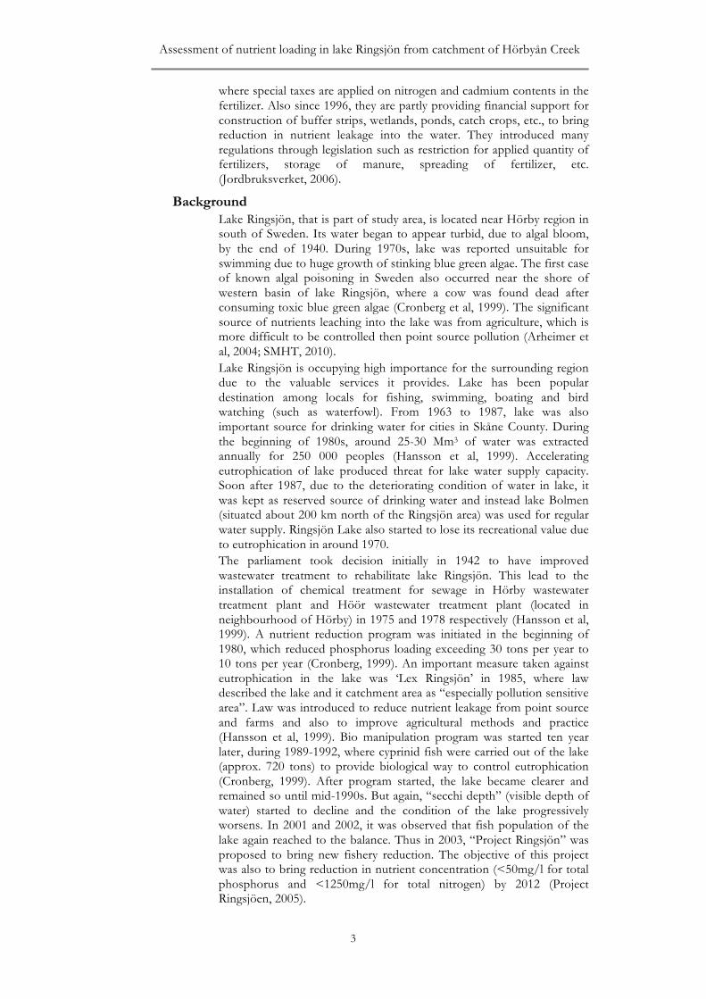
HEC RAS overview Modelling system has three main components: 1. River analysis component 2. Data input component 3. Post-processing component (graphics and reporting) These are briefly described in the following paragraphs. 1. River analysis component The river analysis component can perform various hydraulic calculations such as: a. Steady-state water surface profiles b. Unsteady flow simulation c. Sediment transport/movable boundary computations d. Water quality analysis a. Steady-state water surface profiles This component of the model allows calculating water surface profile from steady input discharge data of upstream cross section, using the dimension of river geometry and data for surface roughness for the river (Strehmel, 2011).
Figure 2 : Geometr i c data r epres en ta t ion in HEC RAS.

Assessment of nutrient loading in lake Ringsjön from catchment of Hörbyån Creek
9
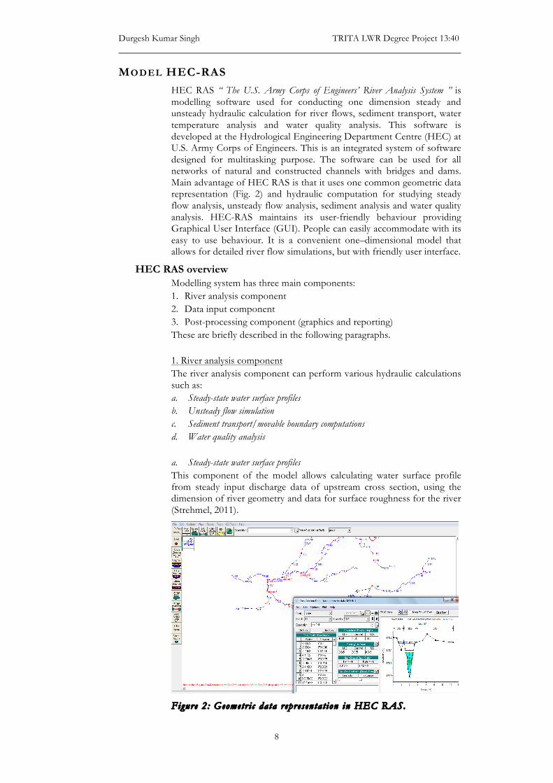
Outputs of this analysis represent the water surface elevation above the base altitude and flow velocity for every cross section. This component is able to work with all kind of flow such as subcritical, supercritical and mixed flow regimes. Computation procedure for steady flow is based upon the solution of the one-dimensional energy equation, where energy losses are evaluated using friction, contraction and expansion. The momentum equation may also be used in case of mixed flow regime, hydraulics of bridges and river confluences. This simulation capability of the model is useful to predict the effect of flow obstructions such as dams, bridges and other hydraulic structures. It has very useful application for flood prediction and control and also flood risk studies. b. Unsteady flow simulation This component of HEC-RAS allows simulating one-dimensional unsteady flow in river networks. The unsteady flow component was initially developed for subcritical flow regimes but it was later extended to mixed flow regime calculations. The computational procedure is based on the solution of the 1D (one-dimensional) Saint-Venant equation for continuity and momentum (Strehmel, 2011). Its components contain special features such as dam break analysis, pumping station, navigation dam operation, pressurized pipe system, levee breaching and overtopping. c. Sediment transport/Movable boundary computations This component of the model is used for the simulation of one dimensional sediment transport and movable boundary calculations over a period of time. The model allows to simulate the behaviour of scouring and deposition of sediments in stream channel resulting from change in frequency, duration of the water discharge and stage or change in geometry. Thus it is helpful tool for evaluating deposition in reservoir, designing channel contraction required for navigation depth maintenance, predicting the effect of dredging on deposition and evaluates the sedimentation in fixed river channels. d. Water quality analysis This component of HEC-RAS allows user to conduct river water quality assessment and estimate water contamination. It allows the user to perform detailed temperature analysis and transport of constituents such as algae, dissolves oxygen, carbonaceous biological oxygen demand, organic phosphorus, orthophosphate, ammonium, nitrate, nitrite and organic nitrogen. This tool can be helpful for conducting nutrient leakage assessment and nutrient transport in rivers. 2. Data input component Date storage is accomplished using flat files such as ASCII, Binary and HEC-DSS (Data Storage System). ASCII and Binary flat files store the user input data under separate categories of project, plan, geometry, unsteady flow, steady flow, sediment data, quasi steady flow and water quality information. Separate Binary files are used for storing output files. Data can also be transferred to other programs using HEC-DSS. Data management is achieved using the user interface (Fig. 3). User is required to give filename in beginning of project and rest of the files are created and named by interface itself. Interface also provides options for moving, deleting and renaming of files according to the requirement of user.
Durgesh Kumar Singh TRITA LWR Degree Project 13:40
10
Figure 3 : The HEC-RAS main window showing the con tro l to a c c e s s var ious module s o f the mode l .
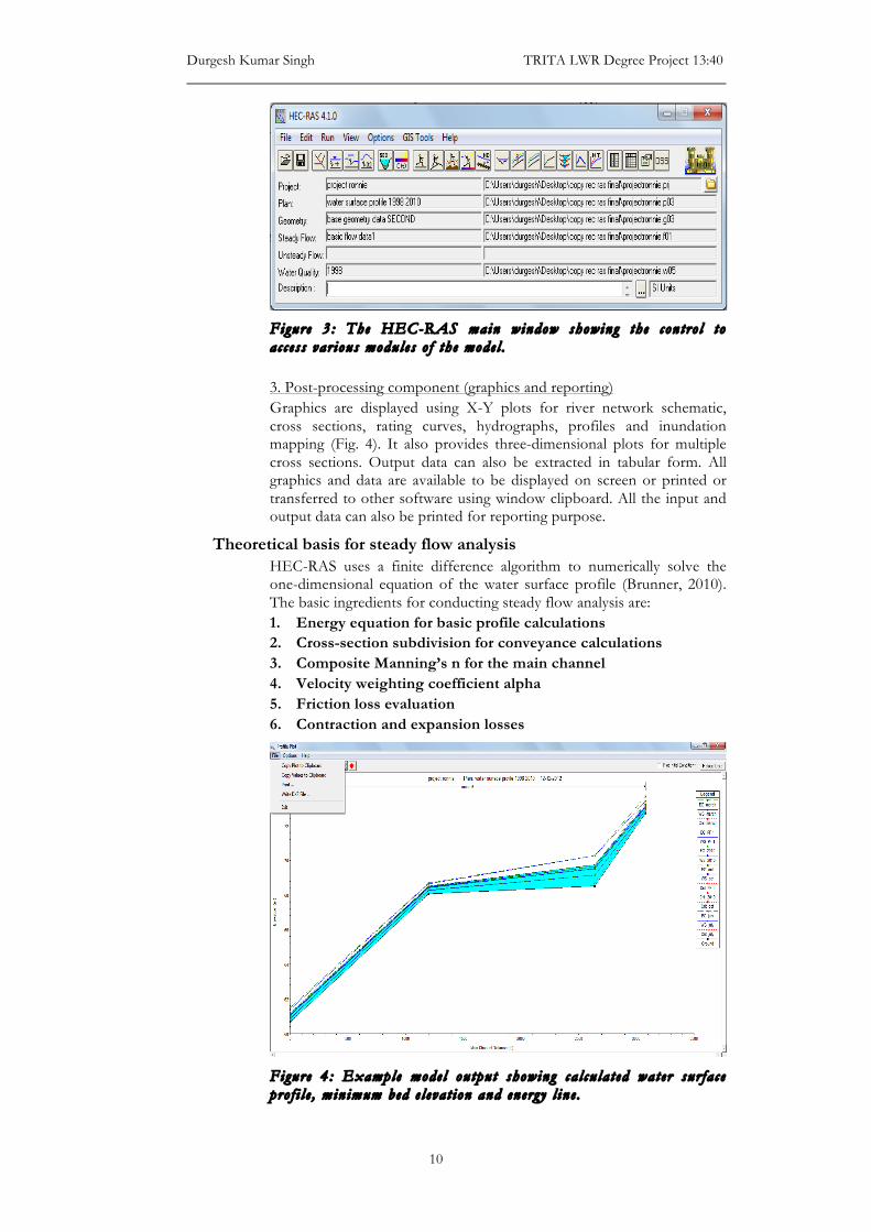
3. Post-processing component (graphics and reporting) Graphics are displayed using X-Y plots for river network schematic, cross sections, rating curves, hydrographs, profiles and inundation mapping (Fig. 4). It also provides three-dimensional plots for multiple cross sections. Output data can also be extracted in tabular form. All graphics and data are available to be displayed on screen or printed or transferred to other software using window clipboard. All the input and output data can also be printed for reporting purpose.
Theoretical basis for steady flow analysis HEC-RAS uses a finite difference algorithm to numerically solve the one-dimensional equation of the water surface profile (Brunner, 2010). The basic ingredients for conducting steady flow analysis are: 1. Energy equation for basic profile calculations 2. Cross-section subdivision for conveyance calculations 3. Composite Manning’s n for the main channel 4. Velocity weighting coefficient alpha 5. Friction loss evaluation 6. Contraction and expansion losses
Figure 4 : Example mode l output showing ca l cu la t ed water sur fa c e pro f i l e , min imum bed e l eva t ion and energy l ine .
Assessment of nutrient loading in lake Ringsjön from catchment of Hörbyån Creek
11
1. Energy equation for basic profile calculations Water surface profiles (Fig. 4) are computed between two cross sections by solving the energy equation:
𝑍! + 𝑌! +𝑎!𝑉!!
2𝑔= 𝑍! + 𝑌! +
𝑎!𝑉!!
2𝑔+ ℎ!
Where, Z1, Z2 = Elevation of the main channel inverts Y1, Y2 = Depth of water at cross sections V1, V2 = Average velocities (total discharge/total flow area) a1, a2 = Velocity weighting coefficients g = Gravitational acceleration he = Energy head loss Energy head loss (he) is evaluated using friction losses and contraction or expansion losses. Thus equation for energy loss is:
ℎ! = 𝐿𝑆! + 𝐶𝑎!𝑉!!
2𝑔−𝑎!𝑉!!
2𝑔
Where, L = Discharge weighted reach length Sf = Representative friction slope between two sections C = coefficient for expansion or contraction loss L is calculated as
L = !!"#!!"#!!!"!!"!!!"#!!"#!!"#!!!"
(1)
Where, Llob , Lch , Lrob = Cross section reach lengths specified for flow in the left overbank, main channel and right over bank, respectively Qlob + Qch + Qrob = Arithmetic average of the flows between sections for the left overbank, main channel and right over bank, respectively 7. Cross section subdivision for conveyance calculations Conveyance is evaluated for cross section sub division using the Manning’s equation
𝑄 = 𝐾𝑆!!!
𝐾 =1.486𝑛
𝐴𝑅! !
Where, K = Conveyance for subdivision n = Manning's roughness coefficient for subdivision A = Flow area for subdivision R = Hydraulic radius for subdivision (area / wetted perimeter) 8. Composite Manning’s n for the main channel For estimating nc, main channel is divided into N parts with known wetted perimeter Pi and roughness coefficient ni
𝑛! =𝑃!𝑛!!.!!
!!!𝑃
! !
Where, nc = Composite or equivalent coefficient of roughness P = Wetted perimeter of entire main channel Pi = Wetted perimeter of subdivision I ni = Coefficient of roughness for subdivision

Durgesh Kumar Singh TRITA LWR Degree Project 13:40
12
9. Velocity weighting coefficient alpha (𝑎) To evaluate the mean kinetic energy it is mandatory to obtain the Velocity weighting coefficient alpha. This alpha is calculated as:
𝑎 =𝐴! ! 𝐾!"#!
𝐴!"#!+ 𝐾!!!
𝐴!!!+ 𝐾!"#!
𝐴!"#!
𝐾!!
Where, At = Total flow area of cross section Alob, Ach, Arob = Flow areas of left overbank, main channel and right over bank, respectively Kt = Total conveyance of cross section Klob , Kch , Krob = Conveyances of left overbank, main channel and right
overbank, respectively 5. Friction loss evaluation Friction loss is evaluated as product of Sf and L. Sf is representative friction for a reach. This can be computed from:
𝑆! =𝑄𝐾
!
L is evaluated from:
𝐿 =𝐿!"#𝑄!"# + 𝐿!!𝑄!! + 𝐿!"#𝑄!"#
𝑄!"# + 𝑄!! + 𝑄!"#
The various variables are explained above in equation (1). 6. Contraction and expansion losses Contraction and expansion losses can be evaluated using following equation:
ℎ!" = 𝐶𝛼!𝑉!!
2𝑔−𝛼!𝑉!!
2𝑔
Where C is the coefficient for contraction or expansion.
Theoretical basis of water quality analysis Theoretical explanation for water quality analysis is well explained in HEC-RAS User’s Manual (Brunner & CEIWR-HEC, 2010) that explains the algorithms used for evaluation of different water quality parameters. This module of HEC-RAS uses the QUICKEST- ULTIMATE explicit numerical scheme to solve the one dimensional advection-dispersion equation. Output of the model is presented in the form of individual sources and sinks as well as computed concentration. This water quality model requires calibration of unsteady or steady flow model before proceeding to water quality module. Following nine state variables are modelled performing water quality analysis: 1. Dissolved Nitrite Nitrogen (NO2) 2. Dissolved Nitrate Nitrogen (NO3) 3. Dissolved Organic Nitrogen (Org N) 4. Dissolved Ammonium Nitrogen (NH4) 5. Dissolved Organic Phosphorus (Org P) 6. Dissolved Orthophosphate (PO4) 7. Algae 8. Carbonaceous Biological Oxygen Demand (CBOD) 9. Dissolved Oxygen (DOX)

Assessment of nutrient loading in lake Ringsjön from catchment of Hörbyån Creek
13
These variables affect each other depending upon rate constants between them. These rate constants define the physical and chemical reactions between different water quality variables and control the rate of source and sink term (S) in the advection-dispersion equation given below (Brunner & CEIWR-HEC, 2010):
𝛿𝛿𝑡
𝑉𝜙 = −𝛿𝛿𝑥
𝑄𝜙 𝛥𝑥 +𝛿𝛿𝑥
𝛤𝐴𝛿𝜙𝛿𝑥
𝛥𝑥 ± 𝑆
V = Volume of water quality cell (m3) ϕ = Temperature of water (C) or concentration of different parameters (kg m-3) Q = Flow discharge (m3 s-¹) 𝛤 = Dispersion coefficient (m2 s-¹) A = Cross sectional area (m2) S = Sources and sinks for various water quality variables (kg s-¹)
Temperature Dependence of Rate Reactions Many of the reactions between variables are temperature dependent. This relationship between reactions rate and temperature is evaluated using Arrhenius rate law.
𝑘! = k₂₀ 𝜃 ⁽ᵀ ⁻²⁰⁾
Where, 𝑘! = Rate constant at temperature T k₂₀ = Rate constant at 20 ͦC 𝜃 = Temperature correction coefficient (it is set to 1.024 and 1.047 for physical and chemical reactions respectively in this model)
Algae Nutrient concentrations (such as NH4, NO3, PO4, Org N and Org P), dissolved oxygen and algal mass are affected due the algal growth and respiration. Algal respiration consumes dissolved oxygen during the night and algal photosynthesis releases dissolved oxygen during the day. Algae consume inorganic phosphorus and nitrogen (such as NH4, NO3 and PO4) and in return releases organic nitrogen and phosphorus back to environment. Algal Biomass Concentration (A) Algal biomass concentration is evaluated using two sinks and one source for it. Source for algal biomass is algal growth, whereas sinks are algal respiration and settling. Thus sources and sink can be estimated by:
A source/sink = 𝐴𝜇∗ (algal growth) -‐ 𝐴𝜌∗ (algal respiration) -‐ !!∗
!𝐴 (algal
settling)
Where, 𝜌∗= Algal local respiration rate (day-¹), which is temperature dependent process. It combines the endogenous algal respiration and conversion of algal nitrogen and algal phosphorus into organic nitrogen and organic phosphorus respectively. 𝜎1* = Algal settling rate (m day -¹), a temperature dependent process d = Average depth of the channel (m) 𝜇 = Local growth rate for algae (day -¹) 𝜇 can be evaluated by
𝜇 = 𝜇!"#∗ 𝐺𝐿

Durgesh Kumar Singh TRITA LWR Degree Project 13:40
14
Where, 𝜇 max* = Local maximum growth rate for algae GL = algal specific growth rate limitation, which is function of nutrient (nitrogen and phosphorus) and light availability Algal specific growth rate calculation (GL) Algal growth rate is evaluated using either of following two limitation functions for growth rate: Leiberg’s Limiting Nutrient or the multiplicative formulation. Leiberg’s Limiting Nutrient According to Leiberg’s Law, algal growth is limited by availability of light and the nutrient that is least available among nitrogen and phosphorus.
GL = FL min (FP, FN)
Where, FL = Limitation for light FP = Limitation for phosphorus FN = Limitation for nitrogen The multiplicative formulation This formulation considers light and availability of both nutrients for algal growth rate.
GL = FL FP FN
Nutrient limitation for nitrogen (FN) Nutrient limitation for nitrogen is evaluated using Michaelis-Menton nitrogen half-saturation constant (KN) and concentration of ammonium and nitrates in water, where KN specifies the phytoplankton efficiency to consume nitrogen at lower concentration.
𝐹𝑁 =𝑁𝑒
𝑁𝑒 + 𝐾𝑁
Where, Ne = Local concentration of available inorganic nitrogen, which can be evaluated from Ne = (NH4) + (NO3) KN = Michaelis-Menton nitrogen half-saturation constant (mg N L-¹) Nutrient Limitation for Phosphorus (FP) Value for nutrient limitation for phosphorus is evaluated using Michaelis-Menton phosphorus half-saturation constant (KP) and concentration of inorganic phosphorus.
𝐹𝑃 =𝑃𝑂!
𝑃𝑂! + 𝐾𝑃
Where, FP = Limitation for phosphorous KP = Michaelis-Menton phosphorus half-saturation constant (mg P L-¹) Limitation for Light (FL) Value for light limitation is estimated from the equation:
𝐹𝐿 =1𝜆𝑑
𝑙𝑛𝐾𝐿 + 𝐼!
𝐾𝐿 + 𝐼!𝑒!!"
Assessment of nutrient loading in lake Ringsjön from catchment of Hörbyån Creek
15
Where, Io = Surface light intensity (W m-2) d = Average depth of the channel (m) 𝜆= Coefficient for light extinction (m-1), which is user set values KL = Light half saturation constant which defines the level of light at which algal growth is half of the maximum growth rate Surface light intensity (Io) is evaluated from short wave radiation and short wave radiation attenuation coefficient (qsw) (qsw set to 0.50 in model):
𝐼! = 𝑎!"𝑞!" Where, qsw = Short-wave (solar) radiation (W m-2) qsw = Short-wave radiation attenuation coefficient
Nitrogen Parameters The various form of nitrogen found in water are dissolved organic nitrogen (Org N), dissolved ammonium nitrogen (NH4), dissolved nitrite nitrogen (NO2), dissolved nitrate nitrogen (NO3) and particulate organic nitrogen. This version of HEC-RAS assumes dissolved ammonium nitrogen in form of NH4, whereas particulate organic nitrogen evaluation is not included in this version. Different forms of nitrogen keep transforming and thus every form of nitrogen act as internal sink and source for others. Organic nitrogen changes into ammonium nitrogen, then to nitrite and nitrate. Algal growth and decay also contribute into sink and source for various forms of nitrogen respectively. Different sources and sinks for various nitrogenous forms are described below in detail. Sources and sinks of dissolved organic nitrogen The only source of organic nitrogen is algal respiration, whereas settling of organic nitrogen on bed and conversion into ammonium nitrogen constitute sink.
OrgNsource/sink = 𝛼!𝜌∗𝐴 (Algal Respiration)
-‐ 𝛽!∗𝑂𝑟𝑔𝑁 (Hydrolysis of OrgN → NH4) -‐ 𝜎!∗𝑂𝑟𝑔𝑁 (Settling)
Where, 𝛼! = Fraction of nitrogen in algal biomass (mgN mgA-¹) 𝜌∗ = Algal local respiration rate (day-1) a temperature dependent process 𝛽!
∗ =Temperature dependent constant for hydrolysis of Org N into ammonium (day-1) 𝜎!∗ = Temperature dependent constant for organic N settling rate (day-1) Sources and sinks of ammonium nitrogen Sinks for dissolved organic nitrogen act as a sources of ammonium nitrogen such as hydrolysis of organic nitrogen, diffusion from riverbed and benthos. Sinks consist of oxidation of ammonium into nitrite and consumption of ammonium by algae.
NH4source/sink = 𝛽!∗𝑂𝑟𝑔𝑁 (Hydrolysis OrgN → NH4)
+ !!∗
! (Diffusion from settling/benthos)
− 𝛽!∗ 1 − 𝑒𝑥𝑝!!"#∙!"# 𝑁𝐻! (Oxidation of NH4 → NO2)

Durgesh Kumar Singh TRITA LWR Degree Project 13:40
16
− 𝐹!𝛼!𝜇𝐴 (Algal uptake)
Where, 𝛽!
∗ = Temperature dependent rate constant for hydrolysis of Org N to ammonium (day-1) 𝛽!
∗ = Temperature dependent rate constant for oxidation of ammonium to nitrite (day-1) 𝜎!∗ = Temperature dependent rate for ammonium diffusion from benthos (mgN m-2 day -¹) d= Average depth of channel (m) 𝜇= Local growth rate for algae (day -¹) 𝛼! = Fraction of nitrogen in algal biomass (mgN mgA-¹) KNR = First order nitrification inhabitation coefficient (mgO-1 L), set to 0.6 GL = Algal growth limitation F1 = Fraction of ammonia consumed by algae, evaluated by:
𝐹! =𝑃!𝑁𝐻!
𝑃!𝑁𝐻! + 1 − 𝑃! 𝑁𝑂!
Where, 𝑃! = Preference factor for ammonia (value vary between 0-1 where 1 indicate algal maximum preference for ammonium and 0 indicate nitrate respectively) Sources and sinks of nitrite nitrogen The only source for nitrite is oxidation of ammonium into nitrite while sink includes oxidation of nitrite into nitrate. NO2 Sources/Sink =� 𝛽!
∗ 1 − 𝑒𝑥𝑝!!"#∙!"# 𝑁𝐻! (Oxidation of NH4 →NO2)
− 𝛽!∗ 1 − 𝑒𝑥𝑝!!"#∙!"# 𝑁𝐻! (Oxidation NO2 → NO3)
Where, 𝛽!
∗ = Temperature dependent rate constant for oxidation of ammonium to nitrite (day-1) 𝛽!
∗ = Temperature dependent rate constant for oxidation of nitrite to nitrate (day-1) KNR = First order nitrification inhabitation coefficient (mgO-1 L) Sources and sinks of nitrate nitrogen Oxidation of nitrite is considered as the only source for nitrate while algal uptake of nitrate is considered as only sink.
NO3 source/sink =𝛽!∗ 1 − 𝑒𝑥𝑝!!"#∙!"# 𝑁𝑂!
(Oxidation of NO2 → NO3)
− (1 − 𝐹!)𝛼!𝜇𝐴 (Algal uptake)
Where, 𝛽!
∗ = Rate constant for oxidation of nitrite to nitrate (day-1) KNR = First order nitrification inhabitation coefficient (mgO-1 L) 𝛼! = Fraction of nitrogen in algal biomass (mgN mgA-1) 𝜇 = Algal local growth rate (day-1) F1 = Fraction of ammonia consumed by algae

Assessment of nutrient loading in lake Ringsjön from catchment of Hörbyån Creek
17
Phosphorus parameters Used version of HEC-RAS estimated two forms of phosphorus, organic phosphorus and inorganic orthophosphate. In nature, common sources of phosphorus are dissolution of rocks and minerals, agricultural runoff, animal metabolic wastages, sewage, etc. Whereas common sinks for phosphorus mainly comprise of algal uptake and settling on the bed. These internal sources and sinks for different form of phosphorus are described below in detail. Sources and sinks of organic phosphorus Algal respiration is found as internal source of organic phosphorus, whereas breakdown of organic phosphorus into orthophosphate and settling into the bed constitute sinks for organic phosphorus.
OrgP source/sink = 𝛼!𝜌 ∗ 𝐴 (Algal respiration)
−𝛽!∗𝑂𝑟𝑔𝑃 (Decay Org P → PO4)
− 𝜎!∗𝑂𝑟𝑔𝑃(Org P settling)
Where, 𝛽!
∗ = Rate constant for oxidation of Org P to PO4 (day-1) 𝜎!∗= Settling rate for organic phosphorus (Org P) (day-1) 𝜌 * = Algal local respiration rate (day-1) 𝛼!= Fraction of phosphorus in algal biomass (mgP mgA-1) Sources and Sinks of Orthophosphate Two sources accounted for orthophosphate are breakdown of organic phosphorus and diffusion from riverbed or benthos. Sink is comprised of algal uptake only.
PO4 source/sink = 𝛽!𝑂𝑟𝑔𝑃 (Decay OrgP → PO4)
+ !!∗
! (Diffusion from benthos) − 𝛼!𝜇𝐴 (Algal uptake)
Where, 𝜎!∗ = Diffusion rate of orthophosphate from Benthos (PO4) (mgP m-2 day-1) 𝛼! = Fraction of phosphorus in algal biomass (mgP mgA-1) 𝜇 = Local growth rate for algae (day-1) d = Average depth of channel (m)
Carbonaceous Biological Oxygen Demand (CBOD) Loss of CBOD is evaluated from two sinks – settling and decay (oxidation).
CBOD source/sink = -‐ K1CBOD (oxidation) -‐ K3CBOD (settling)
Where, K1* = Temperature dependent rate coefficient for deoxygenation (day-1) K3* =Temperature dependent rate of loss of carbonaceous BOD from settling (day-1)
Dissolved Oxygen (DOX) Sources for dissolved oxygen comprise of atmospheric reaeration and photosynthesis. Sinks are comprised of algal respiration, sediment oxygen demand, carbonaceous biological demand, and oxidation of ammonium and nitrite.

Durgesh Kumar Singh TRITA LWR Degree Project 13:40
18
DOX source/sink = K2*(Osat -‐ DOX) (reaeration)
+ 𝐴 𝛼!𝜇 − 𝛼!𝜌 (photosynthesis and respiration)
−K1CBOD (CBOD demand) − !!! (sediment demand)
− 𝛼!𝛽!𝑁𝐻4 (Ammonium oxidation) − 𝛼!𝛽!𝑁𝑂2 (nitrite oxidation)
Where, Osat = Dissolved oxygen concentration at saturation (mgO L -1) 𝛼! = O2 production per unit algal growth (mgO mgA -1) 𝛼! = O2 uptake per unit NH4 oxidized (mgO mgN -1) 𝛼! = O2 uptake per unit NO2 oxidized (mgO mg N -¹) K1* = Temperature dependent Carbonaceous BOD deoxygenation rate (day -¹) K2* = Reaeration transfer rate (day-1), which evaluate the oxygen exchange along the air-water interface K4* = Sediment oxygen demand rate (mg m2 day -1) 𝛽! = Ammonia oxidation rate (day -1) 𝛽! = Nitrite oxidation rate (day -1) d = Average depth of channel (m)
STUDY AREA Study area is situated in Skåne (Scania in English) County that is Southernmost County of Sweden. Study area is situated approximately between the longitude 13°26’13.99’’E-13°56’30.05’’E and latitude 55°46’27.74’’N-55°55’55.17’’N. Study area is represented by the lake Ringsjön and five neighbour watersheds that pour its water into the lake from southeast direction, through Hörbyån Creek and its tributary streams (Fig. 5). Hörbyån Creek passes though Hörby locality before falling into lake Ringsjön. Big part of area under catchment is used for agriculture followed by forest.
Figure 5 : Study area .

Assessment of nutrient loading in lake Ringsjön from catchment of Hörbyån Creek
19
Lake Ringsjön Lake Ringsjön covers around 40 km² of surface area that consist of three basins: Eastern, Western, and Sätofta Basin (Fig. 5). Their surface area is 20.5 km² for the Eastern Basin, 14.8 km² for the Western Basin and 4.2 km² for the Sätofta Basin. The Lake has 14 tributaries, including the Hörbyån Creek. The Eastern Basin receives discharge from seven tributaries while the Sätofta and Western Basins receive discharge from five and two tributaries, respectively. The study area has been limited to only one of the tributary, Hörbyån Creek, which discharges into the Eastern Basin (Project Ringsjöen, 2005). The water surface elevation of the lake is 53 m above the sea level, and the average depth is 4.7 m. The Eastern Basin has the highest average depth among the three basins of 6.1 m, while the Western and Sätofta Basins have an average depth of around 3.1 m and 3 m, respectively. The maximum depth of the lake is observed in the Sätofta Basin and is around 17.5 m; while the Eastern Basin and Sätofta Basin have a maximum depth of 16.4 m and 5.4 m, respectively. Total volume of lake Ringsjön is 184.2 Mm³. The Eastern Basin represents the largest part of the total volume with 124.8 Mm³, followed by the Western Basin with 46.6 Mm³. The Sätofta Basin is the smallest one with a volume of water around 12.8 Mm³. Total catchment area of the lake is around 347 km², where the Easter Basin accounts for maximum part of it with 221.1 km², whereas the Western and Sätofta Basins have a catchment area of 24.7 km² and 101.7 km², respectively (Hansson et al, 1999).
Hörbyån Creek The tributary Hörbyån Creek is a shallow river that flows into lake Ringsjön from Southeast direction. Hörbyån Creek contributes around 15-20 % of total water discharge into lake Ringsjön from all tributaries (estimated from watershed flow data available (SMHI, 2013)). It flows across the locality of Hörby, which is the only urban region in the catchment. The total length of the Hörbyån Creek and its tributaries is approximately 90 km. The creek has a total catchment area of around 153 km². Hörby wastewater treatment plant is located in watershed 5. The Hörbyån Creek originates in watershed 1 where its small tributary merges into it before entering watershed 3. Its major tributary originating in watershed 2 merges with Hörbyån at the border of watershed 1 and 3. From there it flows through watershed 4 and 5 before falling into the lake Ringsjön (Fig. 5).
Climate Climate in South of Sweden is humid, windy and cold during the winter, whereas it is warm and humid during summer (Hansson, 1999). Temperature reaches around 20 °C (approximate average) during summer, whereas it may be as low as -5 °C (approximate average) during winter (Fig. 6) (WWCI, 2012). In this region the summer lasts for more than 4 months and winter last around 2 months (Encyclopedia of the Nations, 2012). Sunlight is received for around 7 hours in January whereas it increases to 17 hours during the month of July in summer. The annual precipitation in Skåne is around 500-800 mm (Fig. 7) and rarely receives white winters as snow melts down shortly after snowfall in December, January and February (Skåne press, 2012). August is observed to receive maximum precipitation (Fig. 8).

Durgesh Kumar Singh TRITA LWR Degree Project 13:40
20
Figure 6 : Average month ly t emperature (°C) in 2010 (SMHI, 2013) .
Figure 7 : Annual pre c ip i ta t ion (mm) in 1998 and 2010 (SMHI, 2013) .
Figure 8 : Average month ly pre c ip i ta t ion in 2010(mm)(SMHI, 2013) .
Population The population of study area was estimated to be 6721 inhabitants in 1998, which increased to around 7354 in 2010 (Fig. 9) (City Populations, 2012). Most of the population resides in Hörby locality, located in watershed 3, and only a minor part resides in watershed 1, 2 and 4. A small fraction of population also resides in Osbyholm locality that is located in watershed 5.

Assessment of nutrient loading in lake Ringsjön from catchment of Hörbyån Creek
21
Figure 9 : Popula t ion growth in s tudy area .
Watershed division and land use
The study area has five watershed basins as was illustrated in Figure 5. Water accumulated from those watersheds finally discharge into the lake Ringsjön. All watersheds are characterized by difference in size and land use composition (Table 2). Watershed 2 represents largest area under cultivation (43.54 km²) that represents about 52% of total agriculture area in the catchment (Fig. 10) and 72.91% of its own area (Table 2). Agricultural area in watershed 2 is around 38.11 % of its total area. Land in watershed 5 is mostly used for agriculture (94% of the area) but its total size is comparatively smaller than other watersheds (only around 5.98 km²). Watershed 1 contains the largest area of forest cover (47.87 km²), while its rank second for agricultural area, after watershed 2. Urban area is primarily limited to watershed 3.
Table 2 : Watershed compos i t ion , land use and so i l t ype o f the d i f f e r en t water sheds ana ly s ed in th i s s tudy .
Watershed 1 Watershed 2 Watershed 3 Watershed 4 Watershed 5
Total area [km²] 81.685439 59.710718 1.73844 3.694489 6.357195
Land use % km² % km² % km² % km² % km²
Agriculture 38.11 31.13 72.91 43.54 13.02 0.23 75.79 2.8 94.00 5.98
Mosse 2.10 1.72 1.90 1.13 0.00 0 0.00 0 0.00 0
Forestland 58.60 47.87 25.00 14.93 6.90 0.12 0.00 0 0.30 0.02
Urban 0.00 0 0.00 0 14.70 0.26 0.00 0 0.00 0
Other land 1.20 0.98 0.20 0.12 65.40 1.14 24.20 0.89 5.70 0.36
Soil type % km² % km² % km² % km² % km²
Peat 12.22 9.98 10.50 6.27 0.61 0.01 0.31 0.01 0.20 0.01
Fine soil / clay 0.39 0.32 0.52 0.31 0.00 0 0.89 0.03 3.41 0.22
Coarse Ground 9.90 8.09 2.59 1.55 0.00 0 3.20 0.12 1.89 0.12
Moraine 77.20 63.06 86.40 51.59 84.41 1.47 95.59 3.53 94.20 5.99
Thin soils and bare rock 0.20 0.16 0.00 0 15.00 0.26 0.00 0 0.30 0.02
Silt 0.10 0.08 0.00 0 0.00 0 0.00 0 0.00 0

Durgesh Kumar Singh TRITA LWR Degree Project 13:40
22
Figure 10. Agr i cu l ture area under d i f f e r en t water sheds .
METHODOLOGY
Research framework The study was conducted with a scientific approach, starting with literature review along with formulation of project and objective. The literature review provided the necessary guidelines for the continuation and need of study. It helped in analysing the tools and relevant data requirements for the study, defining clear objective and providing basic knowledge for how to conduct this study. The fundamental steps identified for assessing nutrient loading in lake Ringsjön were: 1. Performing steady-state flow and water temperature simulation 2. Usage of the model output for setting up water quality simulations 3. Analysis of water quality simulation output The formulation of research questions was followed by preparation for model setup, data collection and setting up of final model. Results output obtained were analysed with other relevant parameters to achieve the objective. This study followed the given workflow (Fig. 11).
Figure 11. Resear ch workf low.
Research workflow
Defining problem and scope of study Defining problem and scope of study Defining problem and scope of study Defining problem and scope of study
Literature review
Data collection
Model set-up, data input
Model outcome
Analysis of results
Discussion

Assessment of nutrient loading in lake Ringsjön from catchment of Hörbyån Creek
23
Methods and material Preparation for model setup
Setting up of the model to obtain desirable results involved several steps. Primary need was to gather necessary information about initial procedure and data requirement. This step involved a preliminary review of existing literature on the subject, including articles and theses where similar use of HEC-RAS was made. All the necessary guidelines to initiate the steps were provided by HEC-RAS user’s manual. Detailed study of area, using geographical map and river information, helped to avoid unnecessary data set, excess time consumption and helped to create workflow.
Database and data retrieval Data collection was important step as it consumed significant portion of time, depending upon the nature of data. For example metrological data was readily available, but data for nutrient concentration and flow discharge in river were not available. Such data were estimated from other related data and literature review. Thus it was important to know the data requirement during the initial stage of study, both for time management as well as retaining the rhythm of work. HEC-RAS user’s manual was considerably useful to determine the data requirement for conducting study. Data requirement for this study can be specified into three categories:
1. Geometric data 2. Steady flow simulation data 3. Water quality data
1. Geometric data These contain data related to river system schematic, cross section geometry, reach length, Manning’s n value and stream junction information. River system schematic This was the data representing the reaches schematic in geographical plane, describing reaches connection and water flow direction. This data was extracted from river system schematic maps available on websites of Swedish Meteorological and Hydrological Institute (SMHI, 2013). Cross section geometry Cross section geometry represents the ground surface profile of a river at particular location. It is represented by transect profile that is taken at perpendicular direction in horizontal plane with respect to flow direction of river. Different cross sections are usually taken at intervals along the river to characterize the flow carrying capacity of streams. Cross sections are required at representative location throughout the river length and the locations showing significant changes in the property such as discharge, slope, roughness, shape, etc. Each cross section is defined using X-Y data, which indicate the values of station and elevation taken from the direction of left to right bank with respect to watching into downstream direction. This data was obtained from a previously conducted measurement campaign on the same river. Reach length This is the distance between two consecutive cross sections. This data was obtained by georeferencing a map of the study area and using tools in Arc-GIS software. Stream junction data Stream junctions are the location where two or more stream merge together or originate. Stream junction data basically required reach length

Durgesh Kumar Singh TRITA LWR Degree Project 13:40
24
of the stream across the junction point. This was obtained from the map using ArcGIS tools. Manning’s n value The Manning’s roughness coefficient, n, is used in the Manning’s formula for open channel flows. This value was obtained from Manning’s n values given for typical channels in HEC-RAS Reference manual. 2. Steady flow simulation data Simulation of steady flows requires several important data such as flow regime, boundary condition and flow discharge. Flow regime data Water flow in the river is required to be specified either as subcritical flow, supercritical flow or mixed flow. As most natural streams, Hörbyån Creek is characterized by a subcritical slope, thus flow regime of the simulations was assumed to be subcritical. Boundary condition Steady flow simulation requires boundary condition input for estimating the water surface in the upstream and downstream of the river system. Boundary conditions requirement (downstream or upstream) depend upon a flow regime, such as a subcritical flow requires downstream boundary condition, supercritical flow requires upstream flow condition whereas mixed flow regime needs both ends conditions. Boundary condition can be specified using one of the four choices: known water depth elevations, critical depth, normal depth or rating curves. Boundary condition for the study was specified using normal depth that was approximately the slope of the channel bottom. It was evaluated using last two cross sections in downstream. Water discharge Water discharge specifies the rate of water volume flow. Due to subcritical flow regimes in study area, it was specified for upstream boundary. Lateral water inputs were also specified in the model. Water discharge data used for the study were obtained from the web service Vattenwebb, provided by the Swedish Meteorological and Hydrological Institute (SMHI, 2013). 3. Water quality data This part of study required data and information specific to water quality, meteorological conditions, etc. Nutrient parameters Model required boundary conditions for the concentration (mg/L) of water constituents such as algae, dissolved oxygen, carbonaceous BOD (biological oxygen demand), organic nitrogen, nitrate, nitrite, ammonium, orthophosphate, organic phosphorus and temperature. A time series or constant values were required at every flow boundary and upstream of reaches. These data were obtained from Swedish Meteorological and Hydrological Institute (SMHI, 2013). However, data was available only for total nitrogen and total phosphorus loaded from different watersheds. The other concentration parameters were therefore estimated using a number of approximations. Firstly, ratio between different forms of nitrogen and phosphorus components was estimated in total nitrogen and total phosphorus from already measured concentration of fractions in water of the lake (Bergman, 1999). It was used to assume the fraction of different components in total nitrogen and total phosphorus loaded from every watershed. This ratio was used to derive the quantity of different forms of nitrogen and phosphorus
Assessment of nutrient loading in lake Ringsjön from catchment of Hörbyån Creek
25
loaded (in kg) from watershed. As water discharge data was available for every watershed, concentration of different form of nitrogen and phosphorus was estimated for every watersheds outlet. Quantities of nutrient and water in rivers are supposed to increase downstream due to increase in watershed area. Similarly, it was assumed that quantity of various forms of nutrient and water in the Hörbyån Creek would therefore constantly increase with increase in river length. Thus concentration of various forms of nutrients between two points of known concentration in stream was estimated in proportion to the river length. Values for dissolved oxygen, algae concentration and carbonaceous BOD were assumed from pictures recently taken during river survey. As river seemed to have clear water, range of values were assumed for low algae concentration and low carbonaceous BOD, with high dissolved oxygen. Water temperature data A time series or constant values for temperature were also required at every flow boundaries and upstream of reaches to conduct water temperature simulation. Due to limitation for obtaining accurate time series temperature, constant average monthly temperatures were used appropriate to fresh water in Sweden. This data was obtained from previous research conducted in Sweden. Meteorological data In order to obtain water temperature simulation, full meteorological datasets were required. These meteorological datasets were comprised of atmospheric pressure, air temperature, humidity, wind speed, solar radiation and cloudiness. Data such as humidity, air temperature, wind speed were obtained from metrological website (SMHI, 2013), while data for solar radiation and atmospheric was self-calculated by program using the longitude and latitude of the study area. Value for cloudiness was estimated from the data available for cloudy days and radiation from the website of Swedish Meteorological and Hydrological Institute as it was not available in the exact form it was required.
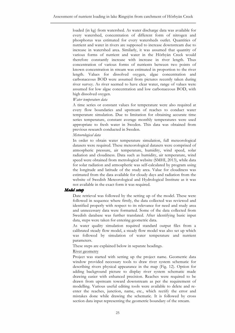
Model setup Date retrieval was followed by the setting up of the model. These were followed in sequence where firstly, the data collected was reviewed and identified properly with respect to its relevance for need and study area and unnecessary data were formatted. Some of the data collected from Swedish database was further translated. After identifying basic input data, steps were taken for entering geometric data. As water quality simulation required standard output files from a calibrated steady flow model, a steady flow model was also set up which was followed by simulation of water temperature and nutrient parameters. These steps are explained below in separate headings. River geometry Project was started with setting up the project name. Geometric data window provided necessary tools to draw river system schematic for describing rivers physical appearance in the map (Fig. 12). Option for adding background picture to display river system schematic made drawing easier with enhanced precision. Reaches were required to be drawn from upstream toward downstream as per the requirement of modelling. Various useful editing tools were available to delete and re-enter the reaches, junction, name, etc., which rectify the error and mistakes done while drawing the schematic. It is followed by cross section data input representing the geometric boundary of the stream.
Durgesh Kumar Singh TRITA LWR Degree Project 13:40
26
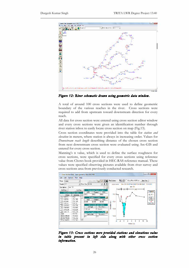
Figure 12: River s chemat i c drawn us ing g eometr i c data window. A total of around 100 cross sections were used to define geometric boundary of the various reaches in the river. Cross sections were required to add from upstream toward downstream direction for every reach. All data for cross section were entered using cross section editor window and every cross sections were given an identification number through river station inbox to easily locate cross section on map (Fig.13). Cross section coordinates were provided into the table for station and elevation in meters, where station is always in increasing order. Values for Downstream reach length describing distance of the chosen cross section from next downstream cross section were evaluated using Arc-GIS and entered for every cross section. Manning’s n value, which is used to define the surface roughness for cross sections, were specified for every cross sections using reference value from Chows book provided in HEC-RAS reference manual. These values were specified observing pictures available from river survey and cross sections area from previously conducted research.
Figure 13: Cross s e c t ions were prov ided s ta t ions and e l eva t ions va lue in tab l e pre s en t in l e f t s id e a long wi th o ther c ross s e c t ion in format ion .
Assessment of nutrient loading in lake Ringsjön from catchment of Hörbyån Creek
27
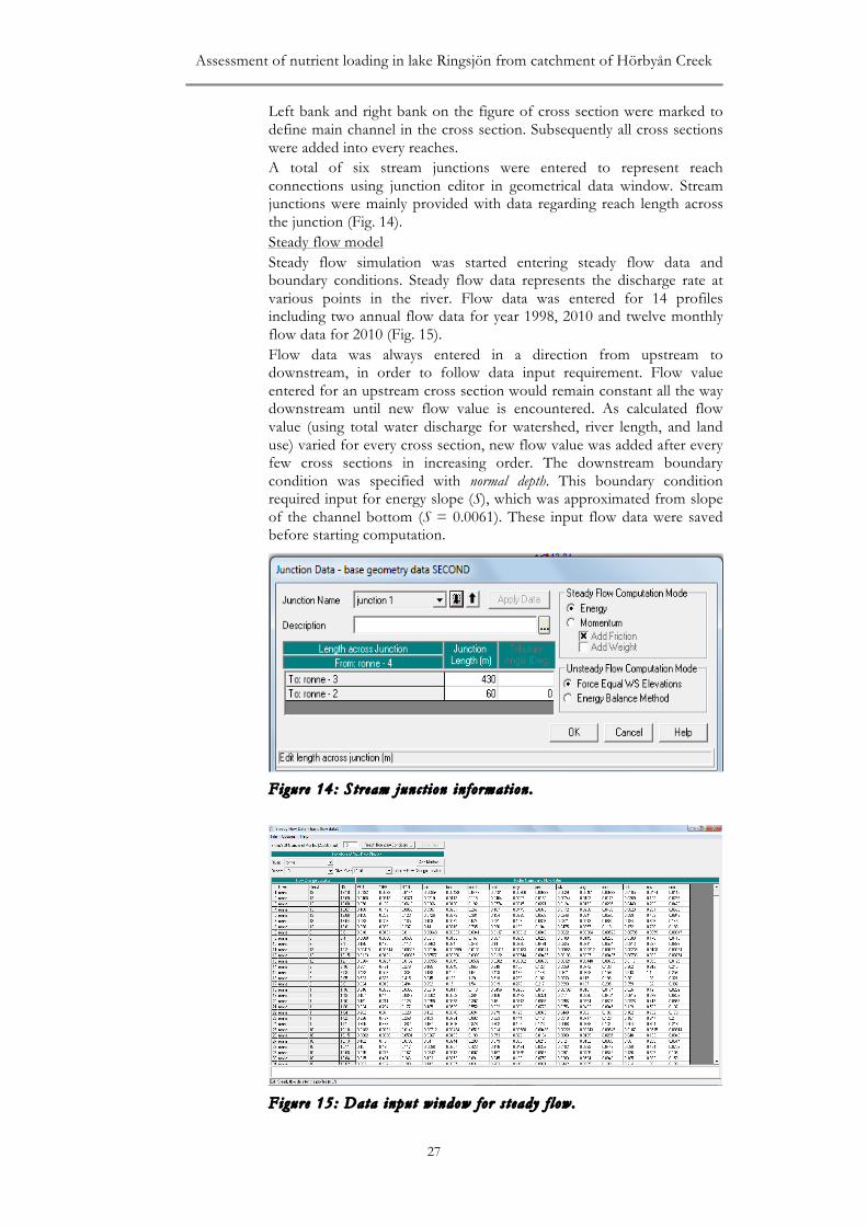
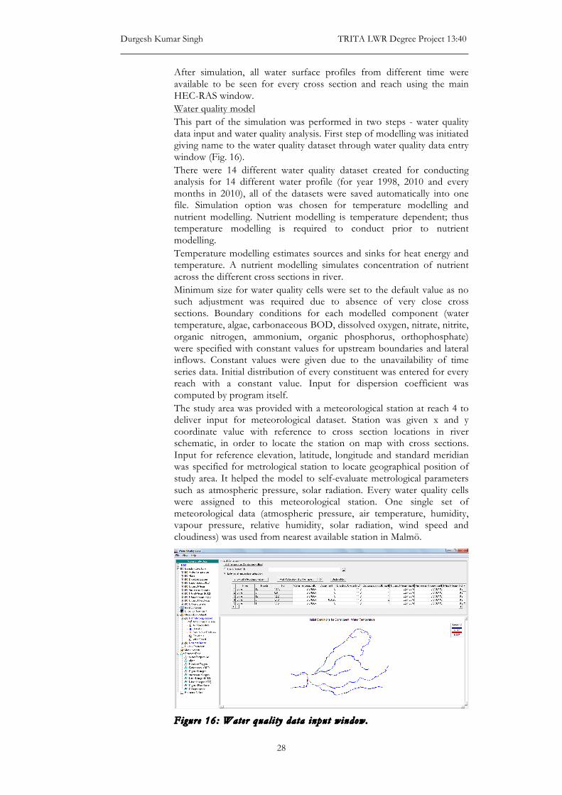
Left bank and right bank on the figure of cross section were marked to define main channel in the cross section. Subsequently all cross sections were added into every reaches. A total of six stream junctions were entered to represent reach connections using junction editor in geometrical data window. Stream junctions were mainly provided with data regarding reach length across the junction (Fig. 14). Steady flow model Steady flow simulation was started entering steady flow data and boundary conditions. Steady flow data represents the discharge rate at various points in the river. Flow data was entered for 14 profiles including two annual flow data for year 1998, 2010 and twelve monthly flow data for 2010 (Fig. 15). Flow data was always entered in a direction from upstream to downstream, in order to follow data input requirement. Flow value entered for an upstream cross section would remain constant all the way downstream until new flow value is encountered. As calculated flow value (using total water discharge for watershed, river length, and land use) varied for every cross section, new flow value was added after every few cross sections in increasing order. The downstream boundary condition was specified with normal depth. This boundary condition required input for energy slope (S), which was approximated from slope of the channel bottom (S = 0.0061). These input flow data were saved before starting computation.
Figure 14: Str eam junc t ion in format ion .
Figure 15: Data input window for s t eady f low.
Durgesh Kumar Singh TRITA LWR Degree Project 13:40
28
After simulation, all water surface profiles from different time were available to be seen for every cross section and reach using the main HEC-RAS window. Water quality model This part of the simulation was performed in two steps - water quality data input and water quality analysis. First step of modelling was initiated giving name to the water quality dataset through water quality data entry window (Fig. 16). There were 14 different water quality dataset created for conducting analysis for 14 different water profile (for year 1998, 2010 and every months in 2010), all of the datasets were saved automatically into one file. Simulation option was chosen for temperature modelling and nutrient modelling. Nutrient modelling is temperature dependent; thus temperature modelling is required to conduct prior to nutrient modelling. Temperature modelling estimates sources and sinks for heat energy and temperature. A nutrient modelling simulates concentration of nutrient across the different cross sections in river. Minimum size for water quality cells were set to the default value as no such adjustment was required due to absence of very close cross sections. Boundary conditions for each modelled component (water temperature, algae, carbonaceous BOD, dissolved oxygen, nitrate, nitrite, organic nitrogen, ammonium, organic phosphorus, orthophosphate) were specified with constant values for upstream boundaries and lateral inflows. Constant values were given due to the unavailability of time series data. Initial distribution of every constituent was entered for every reach with a constant value. Input for dispersion coefficient was computed by program itself. The study area was provided with a meteorological station at reach 4 to deliver input for meteorological dataset. Station was given x and y coordinate value with reference to cross section locations in river schematic, in order to locate the station on map with cross sections. Input for reference elevation, latitude, longitude and standard meridian was specified for metrological station to locate geographical position of study area. It helped the model to self-evaluate metrological parameters such as atmospheric pressure, solar radiation. Every water quality cells were assigned to this meteorological station. One single set of meteorological data (atmospheric pressure, air temperature, humidity, vapour pressure, relative humidity, solar radiation, wind speed and cloudiness) was used from nearest available station in Malmö.
Figure 16: Water qua l i t y data input window.

Assessment of nutrient loading in lake Ringsjön from catchment of Hörbyån Creek
29
A time series data was given for air temperature, humidity and wind speed, while a constant value was used for cloudiness due to data limitation. All of the steps were repeated 14 times to create 14 different water quality data set for different time period (for year 1998 and 2010 and every month in 2010). During the water quality analysis, water quality data were entered along with their respective steady flow profile (same time period) for simulation.
Lumped estimate of nutrient concentrations A theoretical evaluation is also done to estimate the expected average nutrient concentration in different watersheds outlet. This is done for comparison with the HEC-RAS model outcomes. To this end, total nitrogen and total phosphorus concentration is estimated theoretically using the data for flow discharge and nutrient loading from different watersheds outlet (available from Swedish Meteorological and Hydrological Institute (SMHI, 2013)). This dataset available included monthly and annual records for water discharge (in m³/s), total nitrogen (in kg) loaded and total phosphorus (in kg) loaded from different watersheds. Thus expected average annual and monthly nutrients concentration in watersheds outlet was estimated with the following equation:
Nutrient concentration (mg/l) = !"#$% !"#$%&!# !!"#$# !"# !"#$% !"#$ !"#$%& (!" !")!"#$% !"#$% !"#$!!"#$% !"# !"#$% !"#$ !"#$%& (!" !"#$%&)
RESULTS
Model results are presented here only for few representative sites in the river network (Fig. 17). Sites 7, 8, 9 and 10 are located in watershed 1. Sites 1, 2, 3, 4, 5 and 6 are located in watershed 2. Watershed 3, 4 and 5 are represented by sites number 11, 12 and 13 respectively. The results represent annual and monthly water surface profiles, flow discharge and average concentration of nitrogen and phosphorus.
Watershed 1 Watershed 2 Watershed 3 Watershed 4 Watershed 5 Lake
Figure 17: Map o f the s tudy area wi th ind i ca t ion o f var ious s i t e s in the r iv er ne twork cons ider ed in the ana lys i s o f nutr i en t concen tra t ions .
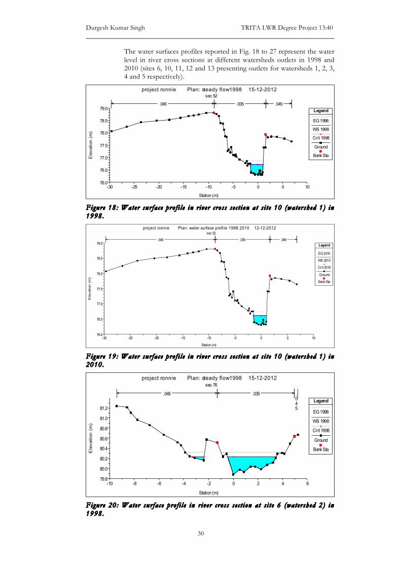
Durgesh Kumar Singh TRITA LWR Degree Project 13:40
30
The water surfaces profiles reported in Fig. 18 to 27 represent the water level in river cross sections at different watersheds outlets in 1998 and 2010 (sites 6, 10, 11, 12 and 13 presenting outlets for watersheds 1, 2, 3, 4 and 5 respectively).
Figure 18: Water sur fa c e pro f i l e in r iv er c ros s s e c t ion a t s i t e 10 (water shed 1) in 1998.
Figure 19: Water sur fa c e pro f i l e in r iv er c ros s s e c t ion a t s i t e 10 (water shed 1) in 2010.
Figure 20: Water sur fa c e pro f i l e in r iv er c ros s s e c t ion a t s i t e 6 (water shed 2) in 1998.
-30 -25 -20 -15 -10 -5 0 5 1076.0
76.5
77.0
77.5
78.0
78.5
79.0
project ronnie Plan: steady flow1998 15-12-2012 sec 52
Station (m)
Ele
vatio
n (m
)
Legend
EG 1998
WS 1998
Crit 1998
Ground
Bank Sta
.045 .035 .045
-30 -25 -20 -15 -10 -5 0 5 1076.0
76.5
77.0
77.5
78.0
78.5
79.0
project ronnie Plan: water surface profi le 1998 2010 12-12-2012 sec 52
Station (m)
Ele
vatio
n (
m)
Legend
EG 2010
WS 2010
Crit 2010
Ground
Bank Sta
.045 .035 .045
-10 -8 -6 -4 -2 0 2 4 679.8
80.0
80.2
80.4
80.6
80.8
81.0
81.2
project ronnie Plan: steady flow1998 15-12-2012 sec 76
Station (m)
Ele
vatio
n (
m)
Legend
EG 1998
WS 1998
Crit 1998
Ground
Bank Sta
.045 .035 .045

Assessment of nutrient loading in lake Ringsjön from catchment of Hörbyån Creek
31
Figure 21: Water sur fa c e pro f i l e in r iv er c ros s s e c t i on a t s i t e 6 (water shed 2) in 2010.
Figure 22: Water sur fa c e pro f i l e in r iv er c ros s s e c t ion a t s i t e 11 (water shed 3) in 1998.
Figure 23: Water sur fa c e pro f i l e in r iv er c ros s s e c t ion a t s i t e 11 (water shed 3) in 2010.
-10 -8 -6 -4 -2 0 2 4 679.8
80.0
80.2
80.4
80.6
80.8
81.0
81.2
project ronnie Plan: water surface profi le 1998 2010 12-12-2012 sec 76
Station (m)
Ele
vatio
n (
m)
Legend
EG 2010
WS 2010
Crit 2010
Ground
Bank Sta
.045 .035 .045
-6 -4 -2 0 2 4 6 860.5
61.0
61.5
62.0
62.5
63.0
63.5
project ronnie Plan: steady f low1998 15-12-2012 sec 59
Station (m)
Ele
vati
on (
m)
Legend
EG 1998
WS 1998
Crit 1998
Ground
Bank Sta
.045 .035 .045
-6 -4 -2 0 2 4 6 860.5
61.0
61.5
62.0
62.5
63.0
63.5
project ronnie Plan: water surface profi le 1998 2010 12-12-2012 sec 59
Station (m)
Ele
vatio
n (
m)
Legend
EG 2010
WS 2010
Crit 2010
Ground
Bank Sta
.045 .035 .045
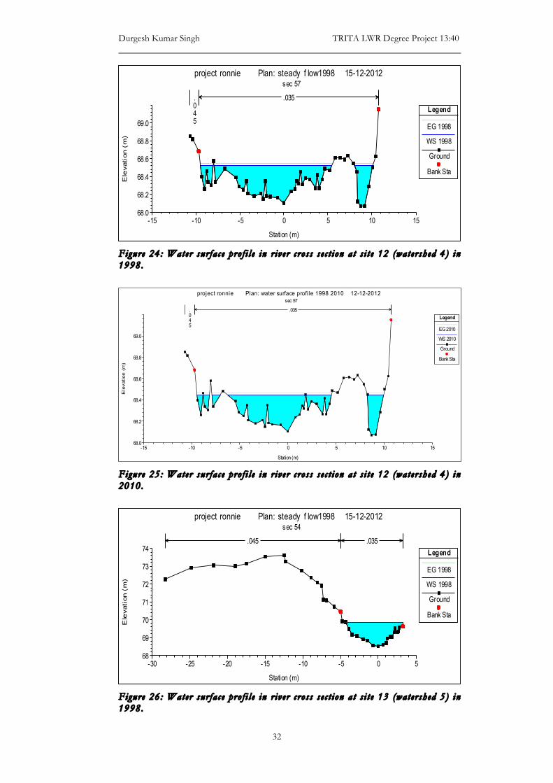
Durgesh Kumar Singh TRITA LWR Degree Project 13:40
32
Figure 24: Water sur fa c e pro f i l e in r iv er c ros s s e c t ion a t s i t e 12 (water shed 4) in 1998.
Figure 25: Water sur fa c e pro f i l e in r iv er c ros s s e c t ion a t s i t e 12 (water shed 4) in 2010.
Figure 26: Water sur fa c e pro f i l e in r iv er c ros s s e c t ion a t s i t e 13 (water shed 5) in 1998.
-15 -10 -5 0 5 10 1568.0
68.2
68.4
68.6
68.8
69.0
project ronnie Plan: steady f low1998 15-12-2012 sec 57
Station (m)
Ele
vati
on (
m)
Legend
EG 1998
WS 1998
Ground
Bank Sta
.045
.035
-15 -10 -5 0 5 10 1568.0
68.2
68.4
68.6
68.8
69.0
project ronnie Plan: water surface profi le 1998 2010 12-12-2012 sec 57
Station (m)
Ele
vatio
n (
m)
Legend
EG 2010
WS 2010
Ground
Bank Sta
.045
.035
-30 -25 -20 -15 -10 -5 0 568
69
70
71
72
73
74
project ronnie Plan: steady f low1998 15-12-2012 sec 54
Station (m)
Ele
vati
on (
m)
Legend
EG 1998
WS 1998
Ground
Bank Sta
.045 .035
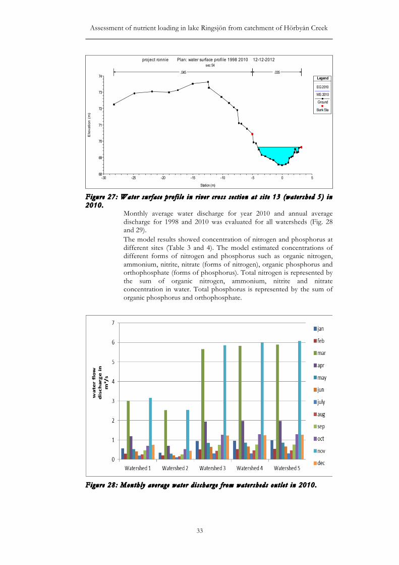
Assessment of nutrient loading in lake Ringsjön from catchment of Hörbyån Creek
33
Figure 27: Water sur fa c e pro f i l e in r iv er c ros s s e c t ion a t s i t e 13 (water shed 5) in 2010.
Monthly average water discharge for year 2010 and annual average discharge for 1998 and 2010 was evaluated for all watersheds (Fig. 28 and 29). The model results showed concentration of nitrogen and phosphorus at different sites (Table 3 and 4). The model estimated concentrations of different forms of nitrogen and phosphorus such as organic nitrogen, ammonium, nitrite, nitrate (forms of nitrogen), organic phosphorus and orthophosphate (forms of phosphorus). Total nitrogen is represented by the sum of organic nitrogen, ammonium, nitrite and nitrate concentration in water. Total phosphorus is represented by the sum of organic phosphorus and orthophosphate.
Figure 28: Month ly average water d i s charge f rom water sheds out l e t in 2010.
-30 -25 -20 -15 -10 -5 0 568
69
70
71
72
73
74
project ronnie Plan: water surface profi le 1998 2010 12-12-2012 sec 54
Station (m)
Ele
vatio
n (
m)
Legend
EG 2010
WS 2010
Ground
Bank Sta
.045 .035
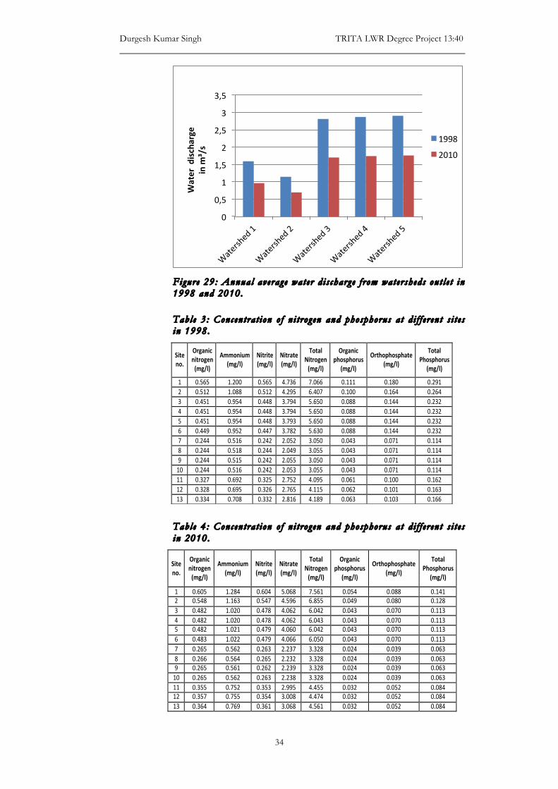
Durgesh Kumar Singh TRITA LWR Degree Project 13:40
34
Figure 29: Annual average water d i s charge f rom water sheds out l e t in 1998 and 2010.
Table 3 : Concentra t ion o f n i t rogen and phosphorus a t d i f f e r en t s i t e s in 1998.
Table 4 : Concentra t ion o f n i t rogen and phosphorus a t d i f f e r en t s i t e s in 2010.
0
0,5
1
1,5
2
2,5
3
3,5
Water discharge
in m
³/s
1998
2010
Site%no.%
Organic%nitrogen%(mg/l)%
Ammonium%(mg/l)%
Nitrite%(mg/l)%
Nitrate%(mg/l)%
Total%Nitrogen%(mg/l)%
Organic%phosphorus%
(mg/l)%
Orthophosphate%(mg/l)%
Total%Phosphorus%%
(mg/l)%
1" 0.565" 1.200" 0.565" 4.736" 7.066" 0.111" 0.180" 0.291"2" 0.512" 1.088" 0.512" 4.295" 6.407" 0.100" 0.164" 0.264"3" 0.451" 0.954" 0.448" 3.794" 5.650" 0.088" 0.144" 0.232"4" 0.451" 0.954" 0.448" 3.794" 5.650" 0.088" 0.144" 0.232"5" 0.451" 0.954" 0.448" 3.793" 5.650" 0.088" 0.144" 0.232"6" 0.449" 0.952" 0.447" 3.782" 5.630" 0.088" 0.144" 0.232"7" 0.244" 0.516" 0.242" 2.052" 3.050" 0.043" 0.071" 0.114"8" 0.244" 0.518" 0.244" 2.049" 3.055" 0.043" 0.071" 0.114"9" 0.244" 0.515" 0.242" 2.055" 3.050" 0.043" 0.071" 0.114"10" 0.244" 0.516" 0.242" 2.053" 3.055" 0.043" 0.071" 0.114"11" 0.327" 0.692" 0.325" 2.752" 4.095" 0.061" 0.100" 0.162"12" 0.328" 0.695" 0.326" 2.765" 4.115" 0.062" 0.101" 0.163"13" 0.334" 0.708" 0.332" 2.816" 4.189" 0.063" 0.103" 0.166"
Site%no.%
Organic%nitrogen%(mg/l)%
Ammonium%(mg/l)%
Nitrite%(mg/l)%
Nitrate%(mg/l)%
Total%Nitrogen%(mg/l)%
Organic%phosphorus%
(mg/l)%
Orthophosphate%(mg/l)%
Total%Phosphorus%%
(mg/l)%
1" 0.605" 1.284" 0.604" 5.068" 7.561" 0.054" 0.088" 0.141"2" 0.548" 1.163" 0.547" 4.596" 6.855" 0.049" 0.080" 0.128"3" 0.482" 1.020" 0.478" 4.062" 6.042" 0.043" 0.070" 0.113"4" 0.482" 1.020" 0.478" 4.062" 6.043" 0.043" 0.070" 0.113"5" 0.482" 1.021" 0.479" 4.060" 6.042" 0.043" 0.070" 0.113"6" 0.483" 1.022" 0.479" 4.066" 6.050" 0.043" 0.070" 0.113"7" 0.265" 0.562" 0.263" 2.237" 3.328" 0.024" 0.039" 0.063"8" 0.266" 0.564" 0.265" 2.232" 3.328" 0.024" 0.039" 0.063"9" 0.265" 0.561" 0.262" 2.239" 3.328" 0.024" 0.039" 0.063"10" 0.265" 0.562" 0.263" 2.238" 3.328" 0.024" 0.039" 0.063"11" 0.355" 0.752" 0.353" 2.995" 4.455" 0.032" 0.052" 0.084"12" 0.357" 0.755" 0.354" 3.008" 4.474" 0.032" 0.052" 0.084"13" 0.364" 0.769" 0.361" 3.068" 4.561" 0.032" 0.052" 0.084"

Assessment of nutrient loading in lake Ringsjön from catchment of Hörbyån Creek
35
Changes in nutrient concentration in the river in 1998 and 2010 Results showed changes in the annual average total nitrogen and phosphorus concentration between 1998 and 2010 (Fig. 30 and 31).
Total nitrogen and phosphorus loading into lake in 1998 and 2010 Results provided estimation of total nitrogen and phosphorus loading into lake Ringsjön (from Hörbyån Creek) in 1998 and 2010 (Fig. 32 and 33).
Figure 30: Change in to ta l n i t rogen concen tra t ion a t d i f f e r en t s i t e s in 1998-2010.
Figure 31: Change in phosphorus concen tra t ion a t d i f f e r en t s i t e s in 1998-2010.
0
1
2
3
4
5
6
7
8
1 (w
atershed
2)
2 (w
atershed
2)
3 (w
atershed
2)
4 (w
atershed
2)
5 (w
atershed
2)
6 (w
atershed
2)
7 (w
atershed
1)
8 (w
atershed
1)
9 (w
atershed
1)
10 (w
atershed
1)
11 (w
atershed
3)
12 (w
atershed
4)
13 (w
atershed
5)
Concen
tra3
on (m
g/l)
Total Nitrogen 1998 (mg/l)
Total Nitrogen 2010 (mg/l)
0
0,05
0,1
0,15
0,2
0,25
0,3
0,35
1 (w
atershed
2)
2 (w
atershed
2)
3 (w
atershed
2)
4 (w
atershed
2)
5 (w
atershed
2)
6 (w
atershed
2)
7 (w
atershed
1)
8 (w
atershed
1)
9 (w
atershed
1)
10 (w
atershed
1)
11 (w
atershed
3)
12 (w
atershed
4)
13 (w
atershed
5)
Concen
tra3
on
mg/l
Total Phosphorus 1998 (mg/l)
Total Phosphorus 2010 (mg/l)
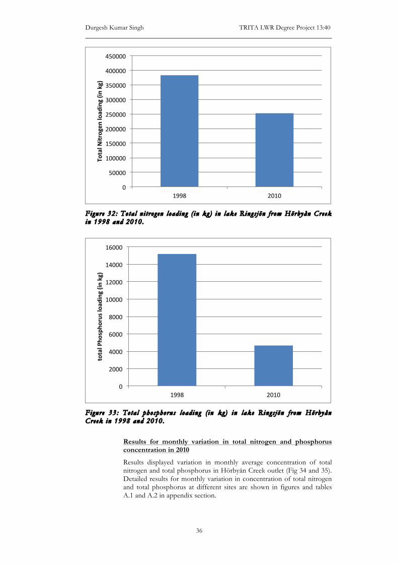
Durgesh Kumar Singh TRITA LWR Degree Project 13:40
36
Figure 32: Tota l n i t rogen load ing ( in kg) in lake Rings jön f rom Hörbyån Creek in 1998 and 2010.
Figure 33: Tota l phosphorus load ing ( in kg) in lake Rings jön f rom Hörbyån Creek in 1998 and 2010.
Results for monthly variation in total nitrogen and phosphorus concentration in 2010
Results displayed variation in monthly average concentration of total nitrogen and total phosphorus in Hörbyån Creek outlet (Fig 34 and 35). Detailed results for monthly variation in concentration of total nitrogen and total phosphorus at different sites are shown in figures and tables A.1 and A.2 in appendix section.
0
50000
100000
150000
200000
250000
300000
350000
400000
450000
1998 2010
Total N
itrogen
load
ing (in
kg)
0
2000
4000
6000
8000
10000
12000
14000
16000
1998 2010
total Pho
spho
rus loa
ding (in kg)

Assessment of nutrient loading in lake Ringsjön from catchment of Hörbyån Creek
37
Figure 34: Average to ta l n i t rogen concen tra t ion (month ly ) a t Hörbyån Creek out l e t in 2010.
Figure 35: Average to ta l phosphorus concen tra t ion (month ly ) a t Hörbyån Creek out l e t in 2010.
DISCUSSION
Results for steady flow analysis (Fig. 18 to 27) indicated reduction in every watershed’s discharge by 39 – 40 % in 2010 with respect to 1998. Consequently, decline in water surface level was observed in year 2010 compared to 1998. Water surface level was found to have declined by 0.1 m to 0.6 m in different watersheds. Maximum decline in water surface level was observed in watershed 2 (0.6 m). This reduced discharge and water surface level was noticeably due to reduced precipitation and runoff in 2010 (Fig. 7). Monthly analysis results indicated that every watershed displayed maximum discharge during November followed by March, whereas minimum discharge was during July (Fig. 28). Precipitation data (Fig. 8) showed small variation with respect to discharge as higher precipitation was observed during August, followed by November. Thus discharge rate did not correspond to precipitation rate in August. It might be
0
1
2
3
4
5
6
7
Concen
tra3
on (in mg/l)
0 0,05 0,1
0,15 0,2 0,25 0,3 0,35 0,4 0,45 0,5
Concen
tra3
on (in mg/l)

Durgesh Kumar Singh TRITA LWR Degree Project 13:40
38
because August received rainfall after a long dry spell (Fig. 8), thus soil might have developed dry and unsaturated condition. This soil condition might have caused complete infiltration of precipitation into ground and resulted into no or little runoff in August. This could have been the possible reason for lower discharge in August, even though receiving higher precipitation. High discharge rate observed in November corresponded to higher precipitation rate in November. During November therefore, most of the precipitation might have turned into runoff due to saturated soil condition from previous precipitation, thus runoff and discharge was increased due to reduced infiltration condition. March showed significantly higher discharge, even though receiving small rainfall. The reason could have been melting of snow on properly saturated soil when temperature increased. It probably resulted into higher runoff and increased discharge due to the condition of reduced infiltration. The minimum discharge observed in July was most likely due the reason of lower precipitation and higher temperature. Higher temperature affects discharge rate by evaporating surface water. The water quality simulation results showed the final outlet of Hörbyån Creek discharging water into lake Ringsjön contained average annual nitrogen concentrations of 4.18 mg/l in 1998 and increased to 4.56 mg/l in 2010 and therefore it indicates 7 – 8 % increase (Fig. 30). Average annual phosphorus concentration in Hörbyån Creek outlet was 0.165 mg/l in year 1998 and reduced to 0.083 mg/l in 2010 and therefore it indicates 49-51 % reduction (Fig. 31). This change was almost same in every watershed. Lake Ringsjön received higher nitrogen and phosphorus loading from Hörbyån Creek in 1998, even with comparatively higher concentration of total nitrogen in 2010. It was primarily due to higher discharge in 1998 (Fig. 32 and 33). Higher volume of water discharged in 1998 carried higher quantity of nitrogen, even though having comparatively lower concentration then 2010. The results from the monthly water quality simulation (Fig. 30 and 31) in 2010, showed that the streams in watershed 2 have the highest total nitrogen concentration, followed by watershed 1. Total nitrogen concentration in streams of watershed 2 was higher than the streams of watershed 1, by approximately 40-50%. Creek’s stream in watershed 3 displayed the average of nitrogen concentration observed in watershed 1 and 2, which is understandably due to the merging of water streams from watershed 1 and 2. Watershed 4 and 5 showed almost similar nitrogen concentration as watershed 3. Total phosphorus concentration shows almost the same pattern as total nitrogen concentration, where creek’s stream of watershed 2 showed highest concentration, followed by watershed 1. Here phosphorus concentration in watershed 2 was higher than watershed 1 by approximately around 30-50%. Same as with nitrogen, phosphorus concentration in watershed 3 displayed total average phosphorus concentration of watershed 1 and 2. Watersheds 4 and 5 had almost similar concentration as watershed 3. Results analysis with land use investigation (Table 2) indicated agricultural area as most important contributor of nutrient. Most of the nutrients were received from watershed 2 that occupied largest agricultural area, followed by watershed 1 that occupied second largest agricultural area. Watershed 1 might also have received some part of nutrients from mineralization of decomposing organic materials in forestland, as watershed 1 also occupied major forestland area. But forestland output was estimated to have lower nutrient leakage with respect to agricultural output. Watershed 2 and 1 was followed by watershed 5, which consists mostly of agricultural area, but because of its

Assessment of nutrient loading in lake Ringsjön from catchment of Hörbyån Creek
39
small size as compared to other watersheds, its nutrient output was not able to bring much effect on nutrient concentration in Hörbyån Creek output. These watersheds were followed by watershed 3 and 4 that were showing least (and almost similar) nutrient output, where most of their lands were used for other purpose. Analysis for the effect of seasonal variability revealed that total nitrogen concentration was highest in every watershed outlet in the month of March, followed by January, April, November, December and February (Fig. 34). November showed significant increase in concentration compared to previous months in the year. This could be justified from the fact that November received comparatively higher precipitation than previous months, except August. August with higher precipitation, followed by lower precipitation in month of September and October possibly made soil well saturated. It probably led to generation of high runoff on already saturated soil, thus much of the nitrogen on surface was easily carried away by high runoff into the stream and resulted into higher concentration. Period from December till February also showed significant higher concentration of total nitrogen but with lower water discharge rate. It was probably due to small runoff and seepage produced from lower precipitation and gradual melting of snow, which probably carried the nitrogen residues from the field. In March, nitrogen concentration was again increased to highest in watersheds outlet, which accompanied with increased water discharge. This could be due to the high runoff produced in March as a consequence of snow melting, which brought additional nitrogen from larger regions. Thus it also brought increase in nutrients concentration. Small runoff in the beginning of April was again bringing remaining nitrogen residues from the field and thus showed significant nitrogen concentration. Total phosphorus concentration was significantly higher in January in every watershed outlet, followed by November and December (Fig. 35). High runoff generated from high rainfall in November might have eroded soil particles bounded with phosphorous from ground and carried it to water streams. Thus it might have increased phosphorus concentration in November. Small runoff and seepage produced from lower precipitation and snow melting in December might have contributed to increased phosphorus concentration in stream in December. Reason for exceptionally high concentration of total phosphorus in January is not well understood, and probably it seems to be simulation error. The values estimated from the lumped model were very useful for assessing HEC-RAS model outcomes. Lumped estimates for the concentration of total nitrogen and total phosphorus in different watershed can be observed in figures A.4 and A.6 (Appendix) that is used to compare with HEC-RAS model results shown in figure A.3 and A.4 (Appendix). This was very useful for assessing the precision of HEC-RAS modelling outcomes. There was some significant deviation in model outcome for nutrient concentration in watershed 5. Total nitrogen concentration obtained in watershed 5 from simulation was higher than expected values from May to October. On the other hand, total phosphorus concentration resulting from the simulations seemed to be higher for every month in watershed 5 with an exceptionally high value for the month of January in every watershed. Apart from that, results from other part of the simulation were reasonably close to the references values. This study was significant to identify the change in nutrient discharge from catchment. It also effectively identified watersheds contribution

Durgesh Kumar Singh TRITA LWR Degree Project 13:40
40
and effect of seasonal variability on nutrient leakage. Study results may not be that accurate for every section of the river network, due to lack of accurate data, but can be considered acceptable for comparative study. This analysis was carried out primarily as a learning opportunity with the aim of developing a distributed stream flow and nutrient transport model for the area of interest. All necessary precaution and attention was taken to achieve a reasonable accuracy in the results but room for error and mistake exists, especially when lot of work was carried out with assumptive values obtained from some related dataset. The results of this work could be more significant if supported by an extensive measurement campaign and if more precise field observations were available. Still this project represents an example application of HEC-RAS for comparative, qualitative and quantitative studies.
CONCLUSION
From the analysis of the results it is concluded that there has been a small reduction in annual average phosphorus concentration in the water of the Hörbyån Creek from 1998 to 2010, but there has been no significant change in annual average nitrogen concentration. Lake still received lower quantity of total nitrogen from in 2010, largely due to lower water discharge in 2010. However, results were not able to clarify reduction in sources of phosphorus in 2010, merely on the basis of the reduction in total average phosphorus concentration. This reduced concentration might have been the result of low rainfall and runoff that showed reduced impact on erosion of soil particles containing phosphorus. However in 2010, phosphorus use was possibly reduced with respect to nitrogen use since 1998, but it cannot be assured. It needs further investigation to confirm such assertion. Concentration of both nutrients (nitrogen and phosphorus) in outflow of Hörbyån Creek was found to have exceeded the referred concentration for eutrophic water in studied year (Table 1). Thus it could be assumed that not much improvement was achieved for nutrient loading from Hörbyån Creek between 1998 and 2010. As the Hörbyån Creek contributes only with around 20% of total water discharged into the lake, nutrient condition of the lake also depends upon other tributary rivers. Yet the contribution of the Hörbyån Creek to the development of eutrophic conditions cannot be disregarded, as it represents a significant amount of the nutrient load into the lake. Among the sub-basins, watershed 2 was observed to be most responsible for nutrient loading (followed by watershed 1), predominantly due to higher area under agriculture. Fertilizers used in agricultural land were primarily the main source of the nutrient but some quantity might also come from the mineralization of crop residues. Most of the nitrogen and phosphorus loading into the lake took place in November and March, which was mainly due to high nutrient concentration in water and high water discharge. For achieving further reduction in nutrient loading, mitigation and measures are required to control nutrient loading from the agricultural areas of watershed 2 and watershed 1. Also technical advancement is required in the field of agriculture for reducing nutrient leakage. Knowledge of the sub-basins that most contribute to nutrient loading, combined with the identification of distributed and point sources of contaminants, should be valuable information for the design of restoration measures and watershed management policies aiming to improve the quality of water in Lake Ringsjön.

Assessment of nutrient loading in lake Ringsjön from catchment of Hörbyån Creek
41
REFERENCES Afeta, A.K., 2006. Assessing Relationships between Stream Water quality
and Watershed Attributes Using the SWAT2000 Integrated Watershed Model - A Case Study in the Ro ̈nne River Basin, Sweden. International Institute for Geo-information Science and Earth Observation, Enschede, The Netherlands. 93p.
Arheimer, B., Andersson, L., Larsson, M., Lindström, G., Olsson, J. & Pers, B.C., 2004. Modelling diffuse nutrient flow in eutrophication control scenarios. Water Science and Technology. Vol 49 No 3 pp 37–45.
Baker, J.L., David, M.B. & Lemke, D.W., 2008. Understanding Nutrient Fate and Transport, Including the Importance of Hydrology in Determining Field Losses, and Potential Implications on Management Systems to Reduce Those Losses. Final Report: Gulf Hypoxia and Local Water Quality Concerns Workshop. American Society of Agricultural and Biological Engineers, St. Joseph, Michigan. Chapter 1, pp. 1-17.
Bergman, E., 1999. Changes in nutrient load and lake water chemistry in Lake Ringsjön, southern Sweden, from 1966 to 1996. L.-A. Hansson & E. Bergman (eds), Nutrient Reduction and Biomanipulation as Tools to Improve Water Quality: The Lake Ringsjön Story. Hydrobiologia 404: pp. 9–18.
Bouraoui, F. & Grizzetti, B., 2011. Long term change of nutrient concentrations of rivers discharging in European seas. The Science of the total environment, 409(23), pp.4899–4916.
Bowie, G.L., W.B. Mills, D.B. Porcella, C.L. Campbell, J.R. Pagenkopf, G.L. Rupp, K.M. Johnson, P.W. Chan, and S.A. Gherini. 1985. Rates, constants and kinetics formulations in surface water quality modeling. 2Ed. EPA/600/3-85/040 U.S. Environmental Protection Agency, Environmental Research Laboratory, Athens GA.
Brunner, G., 2010. HEC RAS, River Analysis System Hydraulic Reference Manual. U.S. Army Corps of Engineers. Hydrologic Engineering Center. 411p.
Brunner, G. & CEIWR-HEC, 2010. HEC-RAS River Analysis System - User Manual Version 4.1. U.S. Army Corps of Engineers. Institute for Water Resources, Hydrologic Engineering Center. 766p.
Cronberg, G., 1999. Qualitative and quantitative investigations of phytoplankton in Lake Ringsjo ̈n, Scania, Sweden. L.-A. Hansson & E. Bergman (eds), Nutrient Reduction and Biomanipulation as Tools to Improve Water Quality: The Lake Ringsjön Story. Hydrobiologia 404: pp. 27–40.
Cronberg, G., Lawton, L.A. & Annadotter, H., 1999. The occurrence of toxic blue-green algae in Lake Ringsjo ̈n , southern Sweden, despite nutrient reduction and fish biomanipulation, L.-A. Hansson & E. Bergman (eds), Nutrient Reduction and Biomanipulation as Tools to Improve Water Quality: The Lake Ringsjön Story. Hydrobiologia 404: pp.123– 129.
Deas, M.L. & Orlob, G.T., 1999. Assessment of Alternatives for Flow and Water Quality Control in the Klamath River below Iron Gate Dam. University of California Davis Center for Environmental and Water Resources Engineering. Report No. 99-04. 236 pp.
Department of Environmental Services (DES), 2010. Lake Eutrophication. Environmental fact sheet. New Hampshire Department of Environmetal Service.
Di, H.J. & Cameron, K.C., 2002. Nitrate leaching in temperate agroecosystems: sources, factors and mitigating strategies. Nutrient Cycling in Agroecosystems 46: 237–256, 2002.

Durgesh Kumar Singh TRITA LWR Degree Project 13:40
42
Hansson, L., Enell, M. & Bergman, E., 1999. Lake Ringsjo ̈n : its catchment area, its history and its importance. L.-A. Hansson & E. Bergman (eds), Nutrient Reduction and Biomanipulation as Tools to Improve Water Quality: The Lake Ringsjön Story. Hydrobiologia 404: pp.1–7.
Jiao, Y., Hendershot, W.H. & Whalen, J.K. 2004. Agricultural Practices Influence Dissolved Nutrients Leaching through Intact Soil Cores. Soil Science Society of America. pp.2058–2068.
Jordbruksverket, 2006. Plan of Action against Plant Nutrient Losses from Agriculture. Swedish Board of Agriculture. 11p.
Khan, F.A. & Ansari, A.A., 2005. Eutrophication : An Ecological Vision. The Botanical Review 71(4): pp.449–482.
Lambooy, T., 2011. Corporate social responsibility: sustainable water use. Journal of Cleaner Production, 19(8), pp.852–866.
Longe, E. & Omole, D., 2008. An Assessment of the Impact of Abattoir Effluents on River Illo, Ota, Nigera. Journal of Environmental Science and Technology 1(2), pp.56–64.
Jørgensen, S. 2001. Water Quality: The Impact of Eutrophication. Lakes and Reservoirs vol. 3. 26p.
McKague,K., Reid,K. & Simpson, H., 2005. Environmental impacts of nitrogen use in agriculture. Ontario Ministry of agriculture and food. 3p.
Strehmel, A., 2011. Model-based hydraulic analysis of flow and sediment transport in the Changjiang basin in the Poyang lake region, China. Institute for Natural Resource Conservation. Department of Hydrology and Water Resources Management.
Tomas, R., Meybeck, M. & Beim, A., 1996. Lakes (Chapter 7) - Water quality assessments: A guide to the use of biota, sediments and water in environmental monitoring, 2nd ed. United Nations educational, Scientific and Cultural Organization World Health Organization United Nations Environment Programme. 651p.
Yang, X., Wu, X., Hao, H. & He, Z., 2008. Mechanisms and assessment of water eutrophication. Journal of Zhejiang University Science. pp.197-209.
OTHER REFERENCES Aberystwyth University, 2013. Nutrients in rivers. Available at
http://www.aber.ac.uk/en/media/03ch10.pdf [Accessed January 17, 2013].
ASA Analytics, 2013. Total Nitrogen in Wastewater. Available at: http://www.asaanalytics.com/total-nitrogen.php [Accessed January 14, 2013].
City Populations, 2012. Osbyholm (Hörby, Skåne, Sweden). Available at: http://www.citypopulation.de/php/sweden-skane.php?cityid=3636 [Accessed December 13, 2012].
Encyclopedia of the Nations, 2012. Climate Sweden Available at: http://www.nationsencyclopedia.com/Europe/Sweden-CLIMATE.html#b [Accessed December 13, 2012].
Experimental Lake Area (ELA), 2012. Eutrophication (Nutrient Pollution) Available at: http://www .experimentallakesarea.ca/images/Eutrophication.pdf [Accessed December 13, 2012].
CSREES North Carolina, 2013. Phosphorus. Extension Water Quality Information System. Available at

Assessment of nutrient loading in lake Ringsjön from catchment of Hörbyån Creek
43
http://www.water.ncsu.edu/watershedss/info/phos.html [Accessed January 28, 2013].
Project Ringsjöen, 2005. Ringsjöen fakta. Available at: http://www.ringsjon.se/ringfakta.asp, [Accessed December 13, 2012].
Skåne press, 2012. Skåne’s geography and climate. Available at: http://press.skane.org/en/content/skanes-geography-and-climate [Accessed December 13, 2012].
Swedish Meteorological and Hydrological Institute (SMHT, 2010) “Why Is Eutrophication Such a Serious Pollution Problem” Available at: http://www.smhi.se/en/theme/sources-of-over-fertilisation-1.12259 [Accessed December 13, 2012].
Swedish Meteorological and Hydrological Institute (SMHI), 2013. Modelarea. Vattenwebb. Available at: http://vattenwebb.smhi.se/modelarea2012/ [Accessed February 17, 2013].
The Michigan Riparian (TMR, 1996) “Lake Classification Systems part 1” Available at: http://www.mlswa.org/lkclassif1.htm, [Accessed December 13, 2012].
The Secchi Dipin, 2013. Phosphorus. Available at http://www.secchidipin.org/Phosphorus.htm [Accessed January 30, 2013].
United Nations Institute for Training and Research (UNITAR) 2013. Nitrogen. Available at: http://www2.unitar.org/cwm/publications/cbl/prtr/pdf/cat5/nitrogen.pdf [Accessed January 4, 2013].
United States Environmental Protection Agency “Total Nitrogen” (EPA, 2013). Available at http://www.epa.gov/region9/water/tribal/training/pdf/TotalNitrogen.pdf [Accessed January 14, 2013].
World Weather and Climate Information (WWCI), 2012. Average weather in Malmö, Sweden. Available at: http://www.weather-and-climate.com/average-monthly-Rainfall-Temperature-Sunshine,malmo,Sweden [Accessed December 13, 2012].

Durgesh Kumar Singh TRITA LWR Degree Project 13:40
44
APPENDIX – SUPPLEMENTARY INFORMATION Table A.1: Month ly to ta l n i t rogen concen tra t ion (mg/l) a t d i f f e r en t s i t e s in 2010.
Table A.2: Month ly to ta l phosphorus concen tra t ion (mg/l) a t d i f f e r en t s ides in 2010.
Site No.
Jan (mg/l)
Feb (mg/l)
March (mg/l)
April (mg/l)
May (mg/l)
June (mg/l)
July (mg/l)
Aug (mg/l)
Sept (mg/l)
Oct (mg/l)
Nov (mg/l)
Des (mg/l)
1 9.304 6.769 10.055 8.589 2.948 1.740 1.265 0.981 0.856 2.943 7.945 8.080
2 8.435 6.136 9.125 7.787 2.675 1.579 1.148 0.889 0.777 2.668 7.203 7.327
3 7.435 5.408 8.043 6.864 2.356 1.391 1.010 0.784 0.684 2.352 6.349 6.457
4 7.435 5.408 8.043 6.864 2.356 1.391 1.011 0.784 0.684 2.352 6.349 6.457
5 7.435 5.408 8.042 6.863 2.356 1.391 1.010 0.784 0.684 2.352 6.349 6.457
6 7.455 5.409 8.031 6.873 2.357 1.391 1.006 0.786 0.684 2.354 6.339 6.464
7 3.886 3.076 4.946 3.920 1.553 1.093 0.850 0.673 0.693 1.324 3.205 3.480
8 3.886 3.076 4.946 3.920 1.553 1.093 0.850 0.673 0.621 1.324 3.205 3.480
9 3.886 3.076 4.946 3.920 1.553 1.093 0.849 0.673 0.621 1.324 3.205 3.480
10 3.886 3.076 4.946 3.920 1.553 1.093 0.850 0.673 0.641 1.324 3.204 3.480
11 5.212 4.038 6.328 4.963 1.827 1.190 0.906 0.716 0.655 1.751 4.566 4.559
12 5.227 4.041 6.364 4.965 1.816 1.183 0.900 0.710 0.650 1.764 4.594 4.563
13 5.329 4.124 6.457 4.997 1.809 1.178 0.893 0.704 0.647 1.766 4.699 4.620
!
Site No.
Jan (mg/l)
Feb (mg/l)
March (mg/l)
April (mg/l)
May (mg/l)
June (mg/l)
July (mg/l)
Aug (mg/l)
Sept (mg/l)
Oct (mg/l)
Nov (mg/l)
Des (mg/l)
1 0.773% 0.043% 0.111% 0.069% 0.046% 0.047% 0.051% 0.055% 0.055% 0.055% 0.274% 0.132%
2 0.701% 0.039% 0.100% 0.063% 0.042% 0.043% 0.047% 0.050% 0.050% 0.049% 0.248% 0.120%
3 0.618% 0.034% 0.088% 0.055% 0.037% 0.038% 0.041% 0.044% 0.044% 0.043% 0.219% 0.106%
4 0.609% 0.034% 0.088% 0.055% 0.037% 0.038% 0.041% 0.044% 0.044% 0.044% 0.219% 0.106%
5 0.615% 0.034% 0.088% 0.055% 0.037% 0.038% 0.041% 0.044% 0.044% 0.043% 0.219% 0.106%
6 0.617% 0.034% 0.088% 0.055% 0.037% 0.038% 0.041% 0.044% 0.044% 0.044% 0.218% 0.106%
7 0.328% 0.027% 0.053% 0.033% 0.025% 0.027% 0.032% 0.033% 0.032% 0.030% 0.120% 0.068%
8 0.328% 0.027% 0.053% 0.033% 0.025% 0.027% 0.032% 0.033% 0.032% 0.030% 0.120% 0.068%
9 0.328% 0.027% 0.053% 0.033% 0.025% 0.027% 0.032% 0.033% 0.032% 0.030% 0.120% 0.068%
10 0.328% 0.027% 0.053% 0.033% 0.025% 0.027% 0.032% 0.033% 0.032% 0.030% 0.120% 0.068%
11 0.436% 0.030% 0.069% 0.041% 0.029% 0.030% 0.035% 0.038% 0.036% 0.036% 0.163% 0.082%
12 0.773% 0.043% 0.111% 0.069% 0.046% 0.047% 0.051% 0.055% 0.055% 0.055% 0.274% 0.132%
13 0.701% 0.039% 0.100% 0.063% 0.042% 0.043% 0.047% 0.050% 0.050% 0.049% 0.248% 0.120%
!

Assessment of nutrient loading in lake Ringsjön from catchment of Hörbyån Creek
45
Figure A.1: Month ly n i t rogen concen tra t ion a t d i f f e r en t s i t e s in 2010.
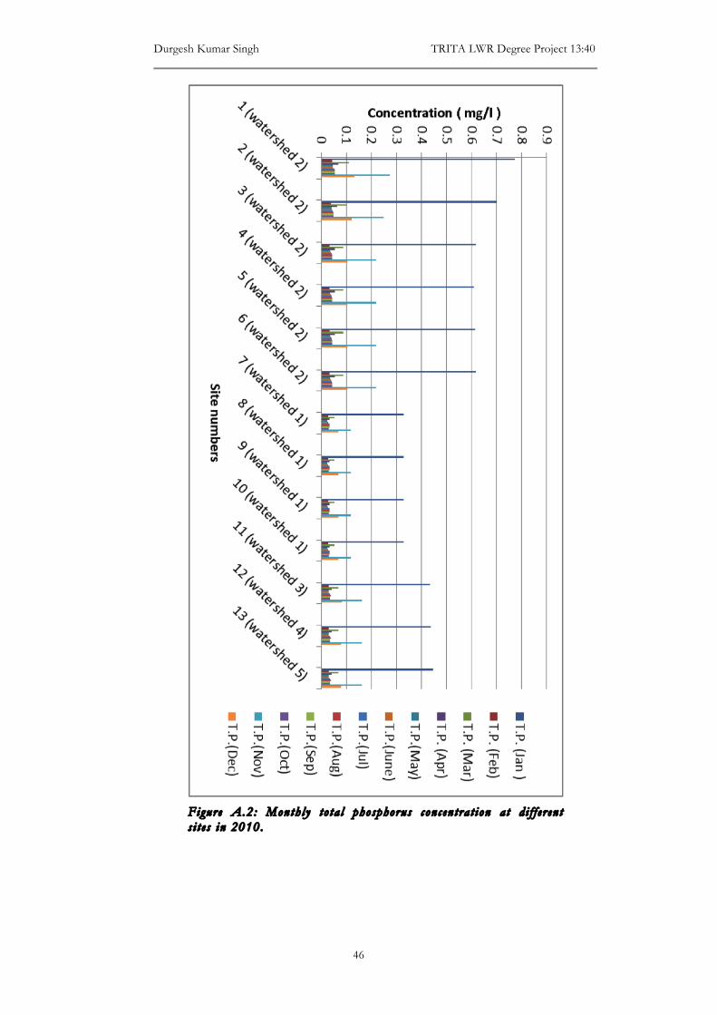
Durgesh Kumar Singh TRITA LWR Degree Project 13:40
46
Figure A.2: Month ly to ta l phosphorus concen tra t ion a t d i f f e r en t s i t e s in 2010.

Assessment of nutrient loading in lake Ringsjön from catchment of Hörbyån Creek
47
Figure A.3: HEC-RAS mode l r e su l t s fo r n i t rogen concen tra t ion in water sheds in 2010.
Figure A.4: Lumped e s t imate r e su l t s fo r n i t rogen concen tra t ion in water sheds in 2010.
0
1
2
3
4
5
6
7
8
9
watershed 1
watershed 2
watershed 3
watershed 4
watershed 5
Concen
tra3
on
mg/l
T.N. (Jan )
T.N. (Feb)
T.N. (Mar)
T.N. (Apr)
T.N.(May)
T.N.(June)
T.N.(Jul)
T.N.(Aug)
T.N.(Sep)
T.N.(Oct)
T.N.(Nov)
T.N.(Dec)
0
1
2
3
4
5
6
7
8
9
watershed 1
watershed 2
watershed 3
watershed 4
watershed 5
Concen
tra3
on
mg/l
T.N. Jan
T.N. Feb
T.N. Mar
T.N. Apr
T.N. May
T.N. Jun
T.N. Jul
T.N. Aug
T.N. Sep
T.N. Oct
T.N. Nov
T.N. Dec

Durgesh Kumar Singh TRITA LWR Degree Project 13:40
48
Figure A.5: HEC-RAS mode l r e su l t s fo r phosphorus concen tra t ion in water sheds in 2010.
Figure A.6: Lumped e s t imate r e su l t s fo r phosphorus concen tra t ion in water sheds in 2010.
0
0,1
0,2
0,3
0,4
0,5
0,6
0,7
Concen
tra3
on
mg/l
T.P. Jan
T.P. Feb
T.P. Mar
T.P. Apr
T.P. May
T.P. Jun
T.P. Jul
T.P. Aug
T.P. Sep
T.P. Oct
T.P. Nov
T.P. Dec
0
0,05
0,1
0,15
0,2
0,25
Concen
tra3
on
mg/l
T.P. Jan
T.P. Feb
T.P. Mar
T.P. Apr
T.P. May
T.P. Jun
T.P. Jul
T.P. Aug
T.P. Sep
T.P. Oct
T.P. Nov
T.P. Dec