ASSESSMENT OF SERVER LOCATION ON SYSTEM AVAILABILITY BY COMPUTER SIMULATION

by

Eric Weissmann

Report submitted to Graduate Faculty of the

Virginia Polytechnic Institute and State University

in partial fulfillment of the requirements for the degree of

APPROVED:

B. S. Blanchard

MASTER OF SCIENCE

in

Systems Engineering

March, 1994

Blacksburg, Virginia

LD 5£55 V<tSJ

1erq1.-1

W"1S/ C,1-,

ACKNOWLEDGMENTS

The author wishes to thank Professors W.J. Fabrycky, B.S. Blanchard and E.R. Clayton for their time and assistance in the completion of this project and report. The author would also like to thank R. Hunter Nichols for his advice during this project.

The author dedicates this book to the memory of his father, Gerd F. Weissmann.

ii

TABLE OF CONTENTS

List of Figures iv

I. INTRODUCTION 1

II. OBJECTIVE AND METHODOLOGY 5 2.1 Objective 5 2.2 Tenninology 5 2.3 Assumptions 6 2.4 Experiment Description 6 2.5 Analytic Calculations For the MTTR 9 2.6 Experiment Procedure 10

Ill COMPUTER SIMULATION 12 3.1 Simulation Software 12 3.2 Program Description 12 3.3 Operation and Verification 13

IV. EXPERIMENT AL RES UL TS AND ANALYSIS 17 4.1 Base Case 17 4.2 Multiple Types Of Distribution 25 4.3 LDT Sensitivity Analysis 28

v. SUMMARY AND CONCLUSIONS 38

References 40

APPENDIX 41

iii

LIST OF FIGURES

Figure 1.1 Basic System Concept 2

Figure 2.1 System Conceptual Design 7

Figure 3.1 Logic Flow Chart 15-16

Figure 4.1 Significant Differences in Availability 18

Figure 4.2 System Availability: Base Case 18

Figure 4.3 Variance of Availability 19

Figure 4.4 Analytic vs. Simulation Availability 20-21

Figure 4.5 Predicted Availability ( Analytic ) 22

Figure 4.6 Travel Distance Output 24

Figure 4.7 Maintainability Results : Base Case 26

Figure 4.8 Server Performance Results 27

Figure 4.9 Base Case vs. Multiple Distribution Availability 29

Figure 4.10 Availability Results : Multiple Distribution 30-31

Figure 4.11 Maintainability Results 32

Figure 4.12 Server Performance Results 33

Figure 4.13 Availability Results: Variable LDT 34

Figure 4.14 Analytic vs. Simulation Availability 35-36

Figure 4.15 Maintainability Results : Variable LDT 37

iv

I. INTRODUCTION

An important characteristic of all systems is availability. Availability is the probability that a

system or piece of equipment will operate in a prescribed manner when used under specified

conditions. It is primarily a design dependent parameter.

Availability derives from a systems reliability and maintainability. Reliability is the probability

that a system will operate for a specified time under specified operating conditions. It is commonly

measured by the mean-time-between-failure (MTBF). Maintainability is the ability of an system to

be maintained. For this report. maintainability is measured by the mean maintenance down time

(MDT). 1

The MDT is a function of several variables, including the mean-time-to-repair (MTIR) and

Logistics Delay Time (LDT). MTIR is the time that active maintenance is being performed. The

LDT is the time delay due to spare part availability, transportation, repair facility availability,

traveling to the location of the malfunction, etc. LDT is a major portion of the MDT. 2

In order to meet a requirement of improved system availability, the MTBF and/or the MDT must

be improved. Decreasing the distance between the repair organization and the location of the

failure may have a significant impact on LDT, assuming that the system's LDT is positively

correlated to the distance traveled. An improvement in the LDT corresponds to an improvement in

the MDT, hence the availability. For a situation where the repair function (referred to as the repair

unit) travels to the location of the failed componen~ the deployment location may have a critical

impact on a system's availability.

In a system where the operating components are located over a wide area and the repair

organization must travel to the component to effect a repair, there are numerous ways to deploy the

servicing units. The systems maintenance concept addresses this issue. The deployment of the

repair units is the central focus of this report.

1 Blanchar~ Benjamin S., Logistics Engineering and Management, 4th Edition, Prentice Hall, Englewood Cliffs, NJ, 1992 2 Blanchard, Benjamin S. and Fabrycky, Wolter J., Systems Engineering and Analysis, 2nd Edition, Prentice Hall, Englewood Cliffs, NJ, 1990

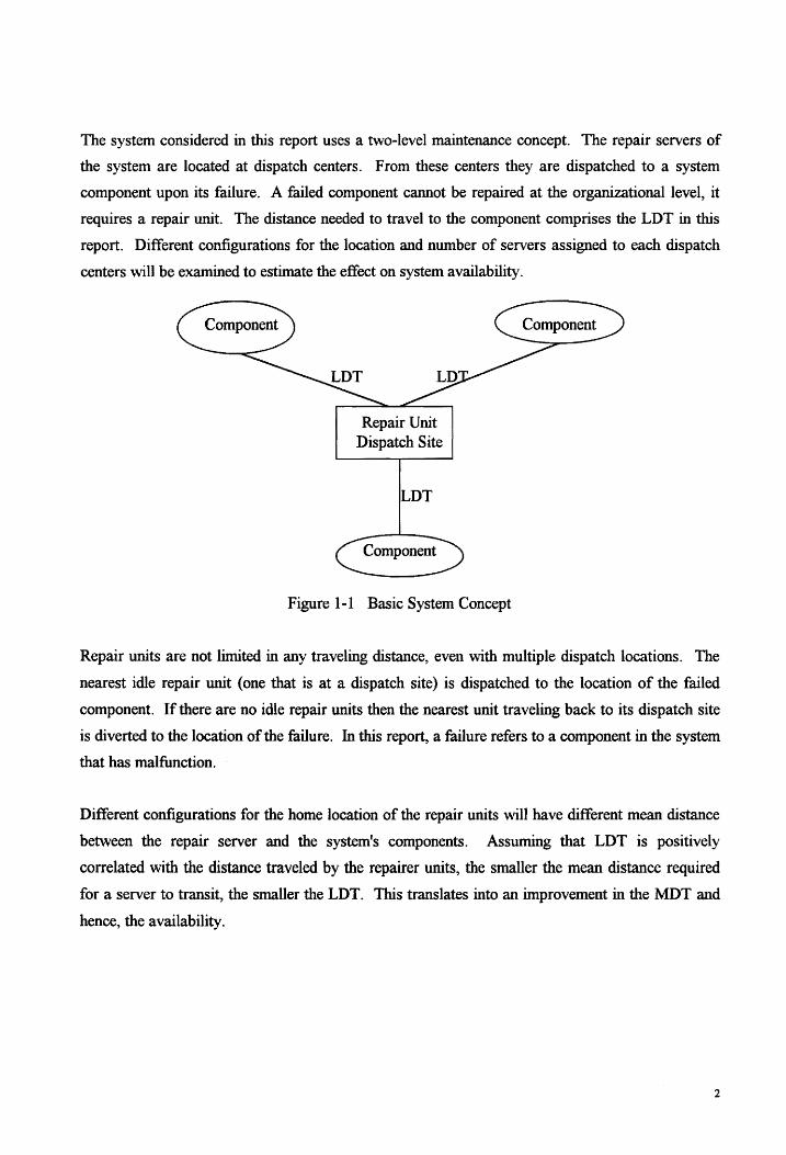
The system considered in this report uses a two-level maintenance concept. The repair servers of

the system are located at dispatch centers. From these centers they are dispatched to a system

component upon its failure. A failed component cannot be repaired at the organizational level, it

requires a repair unit. The distance needed to travel to the component comprises the LDT in this

report. Different configurations for the location and number of servers assigned to each dispatch

centers will be examined to estimate the effect on system availability.

Repair Unit Dispatch Site

LDT

Figure 1-1 Basic System Concept

Repair units are not limited in any traveling distance, even with multiple dispatch locations. The

nearest idle repair unit (one that is at a dispatch site) is dispatched to the location of the failed

component. If there are no idle repair units then the nearest unit traveling back to its dispatch site

is diverted to the location of the failure. In this report, a failure refers to a component in the system

that has malfunction.

Different configurations for the home location of the repair units will have different mean distance

between the repair server and the system's components. Assuming that LDT is positively

correlated with the distance traveled by the repairer units, the smaller the mean distance required

for a server to transit, the smaller the LDT. This translates into an improvement in the MDT and

hence, the availability.

2

It is conjectured that the expected improvements in a systems performance will not be realized.

Randomness in the performance of components, both failure rates and repair rates, may negate the

effects of reducing the mean distance between repair units and components.

The reason for the conjectured lack of improvement is due to some service areas having more

failures that other areas. This situation requires that repair units from other areas travel longer

distances than if all servers were dispatched from a centralized location. An indication of this

occurring in a system would be a large variance for the distance travel by a repair server.

This behavior in the system emphasizes the importance of considering the distribution of input

factors on system performance. Mean values of systems characteristics do not provide a good

indication of how the characteristic is behaving. The variance is an importance descriptor of a

distribution's properties.

By using the variance, a better description is obtained of a system characteristic. A mean value for

performance data does not indicate the range of values or its grouping. The variance of the mean

identifies whether the values are about equal or are very different from one value to the next.

Because of the many interactions of various components, the use of analytic engineering methods is

very difficult and may produce arguable results.3 For many complex systems, analytic solutions

are not possible, or are impractical to solve. Most analytic methods to queuing type problems

usually require ambiguous assumptions, such as exponential behavior in time between arrivals and

servicing times. Accordingly, a computer simulation was developed and its results compared with

results from analytic models.

Computer simulation models yield an estimate of the system's actual characteristics. Deterministic

models result in exact solutions... Computer simulation models may be developed to study complex

designs that cannot be solve by analytic methods.

Another reason for the preference for simulation methods over analytic methods is the ability of

simulation to adapt to different distributions of parameters. The use of distributions as oppose to

3 Law, Averill M. and Kelton, W. David, Simulation Modeling and Analysis, 2nd Edition, McGraw Hill, Inc., New York, NY, 1991 4 lb. Id.

3

just mean values (as in mean-time-between-failure, mean-time-to-repair, etc.) is the consideration

of the effect of variance on inputs and responses. An example of the importance of variance is

given by Law and Kelton (pg. 293).s

Consider a manufacturing system consisting of a single machine tool. Suppose that partS arrive to the machine with an exponential mean of one minute and that processing times are exponentially distributes with a mean of 0.99 minutes. Thus the system is a M/M/l queue with utilization factor of p=0.99. Further more it can be shown that the average delay in queue of a part in the long run is 98.01 minutes. If we replace each distribution by its corresponding mean (i.e., if customers arrive at times I minute, 2 minutes ... and each part has a processing time of exactly 0.99 minutes), then no part is ever delayed in the queue. In general, the variances as well as the means of the input distribution determine the output measures for queuing type systems.

This report will examine the effects on system availability of different configurations of dispersed

servers, where the time required for a server to get to a component is a significant portion of the

total repair time. The objective is to compare the availability forecast by computer simulations and

analytic predictions. Four different server dispatch configurations will be tested.

The system under consideration is a generic and hypothetical system that does not accurately

reflect a particular "real world " system, but has characteristics that may be used by many existing

systems. It could be applicable to a service organization like police or cable installation in a

municipal setting or to a system where the components are deployed worldwide. The basic concept

is that the server must travel to the location where a component has failed. What will the impact

on availability be by adjusting the location from which a server begins a servicing operation? Do

analytic and simulation analysis concur?

5 lb. Id.

4

II. OBJECTIVE AND METHODOLOGY

An evaluation of how the disposition of repair units would effect a systems availability is

performed. Demonstration of sensitivity of system availability to different parameter distributions

and variable Logistic Delay Time (LDT) is evaluated.

2.1 Objective

The objective of this experiment is to compare the system availability for different configurations

of dispersed server dispatch locations. Changes in the systems maintainability will be effected by

the different configurations. Evaluation of the changes in availability due to alterations in

maintainability will be performed.

The system under analysis is a general system consisting of 144 identical components with a repair

organization of sixteen servicing channels. The system and its components are assumed to be in

continuous operation.

2.2 Terminology

For this report the following definitions apply. While some have broader context in systems

engineering, they are limited here to improve description of this project.

• Availability: the probability that a system will be functioning when called upon.6 For this project the system will be assumed to be on call at all times. For this report, availability is measured as the percentage of time that the system has a specified number of functioning components.

• LDT : Logistics Delay Time - time required for a repair units to travel to the location of a failure and return.

• M1TR : Mean-Time-To-Repair - refers to actual time of on site time repairing the failure • MDT : Mean Maintenance-Down-Time - total time that component is out of service;

consists of MTTR and LDT • Length : Distance between two nodes • Dispersal : Used to describe configuration of server dispatch locations • Server : Organization element that accomplishes a repair action

6 Blanchard, Benjamin S., Logistics Engineering and Management, 4th Edition, Prentice Hall, Englewood Cliffs, NJ, 1992

5

2.3 Assumptions

Several assumptions were made to simplify the problem:

• No administrative or other delays • Instant detection of failures • Continuous server operation • All failures are repairable by one server

2.4 Experiment Description

A computer simulation was developed to model a system of widely spread components. The

simulation examines the effects of different dispersal situations on system availability. The mean

reliability of the components comprising the system is held constant. Thus, the major factor

effecting the availability is the maintainability of the system's components.

The system under consideration consists of a population of 144 identical components uniformly

distributed across a service area. There are sixteen identical servers available to repair components

as they fail. Four different dispersal configurations are selected that gave each dispatch location an

equal number of servers assigned. The configurations were for one, two, four, and six.teen dispatch

sites. The site locations were established to minimized the mean distance from site to the

components location in a servers' specified zone.

For conceptual and programming purposes, the system resembles an urban area as in Figure 2.1.

It is a 12 by 12 grid. Each node in the grid represents a component in the system. Dispatch

locations are also located at a node. Travel of the server is on the x and y axis on the lines

connecting the nodes.

Once a component has failed, a server is dispatched from the nearest dispatch site to perform a

repair action. Upon completion of the repair action, the server proceeds to any failed component

that does not have a server assigned. If there are no other failed components, the server starts its

return to its home dispatch location.

6

One Dispatch Site Two Dispatch Sites

_L I T

J. l

1 Dispatch Sites Components

Four Dispatch Site Sixteen Dispatch Sites

. _. -"!

l\ _L

_l If_ 1 .1

_. _. ~ "!

l [ 7 .j _. \ ~

~ -...- -~pr

_. ' 1 "!~ I L .j _. ' ~ 7J /, h_

~ -.,.- ...-

\Y Four Dispatch Sites

Figure 2.1 - System Conceptual Design

7

A server is not required to return to the dispatch site. It is assumed that the server has an unlimited

supply of all material and equipment needed to complete a repair action. No breakdowns or

downtime are incurred by a server. They may remain in continuous operation. Once a particular

server is assigned to a failed component, it is not diverted or replaced, even if a much closer server

becomes available. A server may be diverted on its return to the dispatch site at a node, not while

it is traveling between nodes.

Essentially this system could be modeled as a basic queuing system with sixteen servers. The

MDT is a function of LDT and the MTTR. The time to repair is exponentially distributed, with

constant mean. The LDT is an exponential distribution with a mean that is dependent upon the

distance on the customers' (components) and the servers location. If a queue starts to form, the

mean repair time is also effected, the distance the server must travel is dependent on both the

current and previous location of failed components.

If more than sixteen components are not functional at one time, the system is said to be

unavailable. Sixteen was selected as the threshold of unavailability and is an arbitrary figure. If

more than sixteen components are failed at one time, the system is inoperative or unavailable.

Regardless of the systems status, all operational components continue to operate until failure.

The system has a first-in-first-out queue function for failed components. The first component in

the queue is assigned the first server available, even if another server completes a repair and is

closer to the failed component.

There are two parameters to be considered in the system: reliability and maintainability.

Maintainability consists of the on site MTTR and the LDT. The reliability is measured by the

MTBF. There are three items that are random variables: MTIR, LDT and MTBF.

For a baseline configuration, the mean time to travel between one node was one time unit {TU).

The mean repair time (time at the failure location) was set at 24 TUs. For a single, centralized

dispatch site, the mean distance of a component from the site was six. This equates to a mean

LDT of six TUs. The total MDT= LDT + MTIR = 24 + 6 = 30 TUs. The individual

components set at mean MTBF was 400 TUs for all configurations. The base case was modeled

by sampling exponential distributions only.

8

Additional experiments were performed with different random variable distributions . The time­

between-failures was sampled from a lognonnal distribution7. Its mean remained the same at 400

TU. It had a variance of 200. The LDT remained exponentially distributed with a mean of one.

The MTIR was an Erlang random variable with a shape parameter of two.

The simulation is allowed to run for an initial wann-up phase before statistical data was recorded.

This eliminates the bias caused by all the servers starting from their dispatch sites. After the

wann-up period, many servers are sent directly from one failure to another.

The sensitivity of the system was tested by varying the MTIR. For each of the four dispersal

configurations, the MTIR was varied between 12 and 45 TUs, using 3 TU increments. A total of

12 different mean repair times were used. This results in 48 data points. Each data point was

sampled twenty five times. This was done in order to reduce the variance in the sampling.

Additional sensitivity testing was done by varying the LDT mean. The mean to travel between

nodes was incremented from 0.5 to 3.25 in 0.25 increments. The Repair Time mean was set at 24

TUs for this experiment.

Seven system characteristics were monitored in the experiment; component system MDT, system

MTBF, system availability, server utilization, distance traveled to failure, LDT, and component

MDT.

2.5 Analytic Calculations for the MTTR

The mean distance of a dispatch site to a component is measured from the nearest dispatch site.

Assumptions MTBF =LDT= 1 TU/length MITR=24TU 400TU

7 AT&T Reliability Manual, 1983, Bell Systems Information Publication IP 10475

9

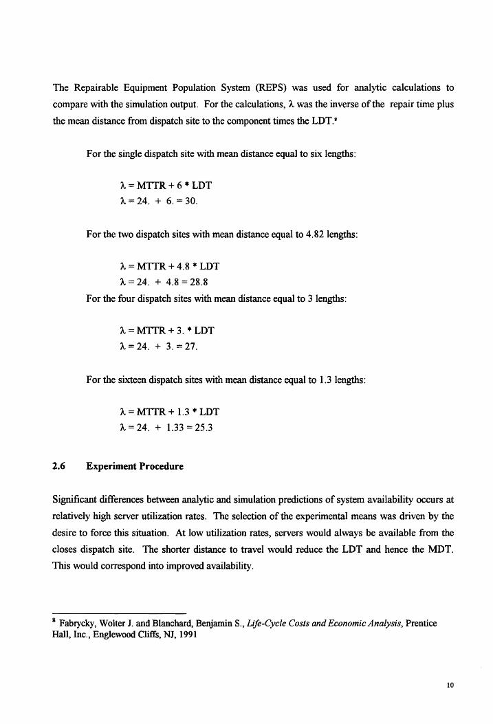
The Repairable Equipment Population System (REPS) was used for analytic calculations to

compare with the simulation output. For the calculations, 1 was the inverse of the repair time plus

the mean distance from dispatch site to the component times the LDT. 8

For the single dispatch site with mean distance equal to six lengths:

1=MTTR+6*LDT

A.= 24. + 6. = 30.

For the two dispatch sites with mean distance equal to 4.82 lengths:

1=MTTR+4.8 *LDT

1=24. + 4.8 = 28.8

For the four dispatch sites with mean distance equal to 3 lengths:

1=MTTR+3.*LDT

1 = 24. + 3. = 27.

For the sixteen dispatch sites with mean distance equal to 1.3 lengths:

1 = MTTR + 1.3 * LDT

1=24. + 1.33 = 25.3

2.6 Experiment Procedure

Significant differences between analytic and simulation predictions of system availability occurs at

relatively high server utilization rates. The selection of the experimental means was driven by the

desire to force this situation. At low utilization rates, servers would always be available from the

closes dispatch site. The shorter distance to travel would reduce the LDT and hence the MDT.

This would correspond into improved availability.

8 Fabrycky, Wolter J. and Blanchard, Benjamin S., Life-Cycle Costs and Economic Analysis, Prentice Hall, Inc., Englewood Cliffs, NJ, 1991

IO

Verification and validation of the model was performed to the extent possible. Since the

simulation modeled a nonexistent system. No validation was possible.

The mean distance for a server to travel from a central dispatch site was calculated as six. The

simulation was run with very high MTBF of the components. This resulted in a very low server

utilization rate. With a server always available for dispatch , the distance traveled output would

result in approximately six lengths. This matched the simulation results within statistically

significant tolerances. Tests were performed on four and sixteen site configurations, with positive

results.

In order to evaluate the diversion of returning servers to failures, write statements were inserted in

the appropriate algorithms. When a diversion occurred, listings of the locations of the servers were

outputted. This output showed that the algorithms were performing as desired.

In order to verify that repair servers were sent from the nearest dispatch site with an available

server, output was obtained by verification methods similar to the diversion testing methods.

This method would not be sufficient for validation of real world simulations. The methods used for

verification in this report is satisfactory because this is a relatively simple, straight forward

simulation.

Standard statistical methods were used to analyze the output. The differences in the availability

compared one dispatch site against the three dispersed dispatch site configurations. The sample

size was sufficiently for valid assumption of the Central Limit Theorem. Statistical testing was a

two tailed, t-distribution test. An a-level of0.05 was used.

MathCad was used to perform REPS and the statistical calculations.

11

III. COMPUTER SIMULATION

A computer simulation model was developed to evaluate the effect of server dispersal on system

availability.

3.1 Simulation Software

The simulation was developed using Simulation Language for Alternative Modeling (SLAM). It

was selected due to the author's familiarity with it, its availability in PC and mainframe computer

systems and its ability to accomplish the desired simulation.

The original model was developed on SLAMSYS for PCs, however it soon outgrew the limitations

and was transferred to the Virginia Tech mainframe. The mainframe version lacks the Windows

graphic capabilities and forces the programmer to increasingly rely on user-defined inserts. These

inserts are written in FORTRAN and make use of numerous SLAM subroutines. The final version

of the model relies heavily on the user inserts, except for creation of entities and scheduling of

events. This is done in the network portion of SLAM. The SLAM and FORTRAN code is in

APPENDIX 1.

3.2 Program Description

The simulation program developed modeled both the components and servers using entities. Each

entity consisted of I 0 attributes. These attributes stored the following values:

Attribute I : time Attribute 2 : component ID Attribute 3 : x coordinate of component Attribute 4 : y coordinate of component Attribute 5 : current x position of server Attribute 6 : current y position of server Attribute 7 : x coordinate of dispatch site Attribute 8 : y coordinate of dispatch site Attribute 9 : server ID Attribute I 0 : Distance from current location to failed component

12

When a component failed, a file of idle servers was searched. The nearest server was selected and

it entered a traveling procedure utilizing Attributes 3-6. If there were no idle servers, a search was

made for any servers returning from a repair operation. If available, the closest available one was

identified and the failed component is placed in a file until its server is diverted. If there were no

servers available, the component was placed in a waiting file.

When a repair action was completed, the component's next failure time was sampled from the

MTBF distribution. The server searches the waiting file for failed components. If one was found,

the Attributes with the components location and ID are copied into the servers attributes. It then

begins a repair cycle. If there are no failed components waiting for a server to become available,

it loads its ID and current location (held in its Attributes 5 and 6) and starts the trip to go its home

dispatch site.

Every time a returning server reaches a node, it checks to see if it is to divert to a failed component,

if it is not required at a failure, it updates its current location and proceeds to the next node. Travel

occurs in an x then y then x axis manner. When the server reaches its home dispatch site, it is

placed in an idle server file.

Figure 3 .1 is the flow chart of the simulation.

3.3 Operation and Verification

Checks were performed to ensure that a steady state condition was achieved in the simulation.

Response variables were sampled at short intervals for multiple runs and different configurations.

Results indicated that the system had achieved a relatively stable condition after 500 TUs.

Additionally, the initial failure times for the components were generated from exponential, Erlang

and uniform distributions. This was done to see that no cycle in the component failures was

induced by the initial system conditions. The output from the different runs showed no significant

difference in the response variables. This indicates that the system has warmed-up. The bias

caused by the initial start-up period has been reduced.

13

Each of the 48 different configurations was run for 125,000 TUs. Sampling was performed every

5000 TU and the statistical arrays were cleared every 2500 TU. This resulted in 25 sampling

operations per configuration.

Output was written to a separate file for use by MathCad.

14

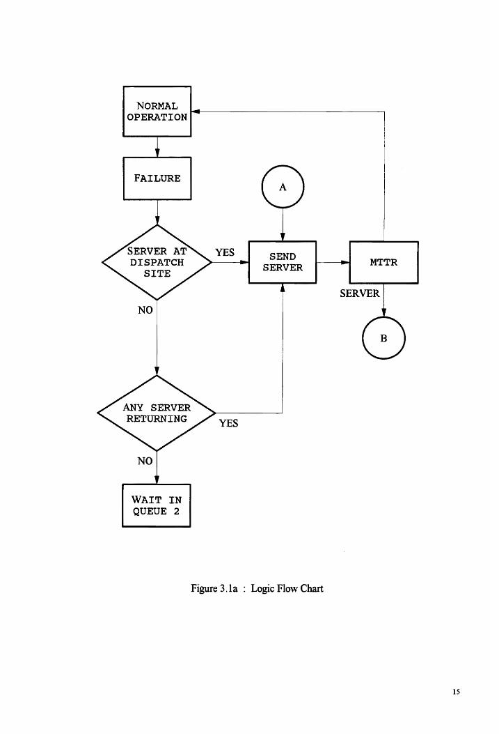
NORMAL OPERATION

FAILURE

NO

NO

WAIT IN QUEUE 2

YES

SEND SERVER

Figure 3. la : Logic Flow Chart

MTTR

SERVER

15

NO

TRAVEL .-----...t 1 LENGTH

(LDT)

NO

YES

WAIT FOR NEXT

FAILURE

YES

YES

Figure 3.lb - Logic Flow Chart

16

IV. EXPERIMENTAL RESULTS AND ANALYSIS

The experimental data did not conclusively support the contention that dispersal of server dispatch

sites would have detrimental effect on system availability. The results gave some evidence of

improved availability by using dispersed server dispatch sites. The most important result was the

lack of improvement in system availability for all the dispersed configurations. The system

availability was significantly effected by varying the MTTR varying the LDT and using different

MTTR and MTBF distributions.

4.1 Base Case

The base case did not indicate any significant change in availability for pair-wise comparisons of

the means for each dispatch site configuration with the same MTTR distribution. Figure 4.1 This

figure is shown to emphasis the lack of significant change in system availability.

Only one data point had significant increase in availability. This was for six.teen dispatch sites and

a mean repair time of 24 TU. Twelve different mean repair times for each of three pair wise

combinations, 36 total comparisons, resulted in only one significant difference. Increasing the level

to 0.20 only yielded three additional points of increased availability. Decreasing the a level to

0. 025 resulted in no data points of change in the availability. The threshold selection of sixteen,

results in availability 100% when the mean repair times is less than 18 TU.

Systems availability was sensitive to the changes in the mean repair time, not the dispersal of

servers throughout the system. The plot of system availability in Figure 4 .2 has relatively

horizontal lines. This indicates that availability is sensitive to changes in mean repair time, not

dispatch site configuration. The change in shade on the y-axis shows the change in availability

with changing mean repair times.

Variance for the availability increases with the repair time as shown on Figure 4.3. The increase

indicates chaos in the system. For repair times of 30 and greater, the variance is large enough to

reduce confidence in conclusions drawn. The variance does not appear to vary widely for different

configurations.

17

z.; 2.s

i 2

l,; l.s 1

l

o.; O.s 0

.,.., -'er"" 4'--. ~ -""-

~--- ...... ~ o~ ~ ..._.. .....

Figure 4 .1 - Significant Differences in Availability

42

18

12-+----------------.--------------..--------------~ 1 Site 2 Sites 4 Sites 16 Sites

Configuration

Figure 4.2 - System Availability : Base Case

~ 1 .... tJ .... .!.

1

0.9

0.8

0.7

0.6

0.5

0.4

0.3

0.2

0.1

0

18

42

36

18

12 1 Site 2 Sites 4 Sites

Configuration

Figure 4.3 - Variance of Availability

16 Sites

0.025

0.02

0.015

0.01

[11:1~ 0.005

~?!~i~ 0

Predicted analytic availability versus the simulation availability is shown in Figures 4.4a and 4.4b.

For one site, the availabilities are nearly identical. There is one point where the simulation results

are better than the analytic, however this point is not statistically significant. For two sites the

results are also almost identical except at high mean repair times.

Figure 4.4b shows where there are significant discrepancies between the analytic and simulation

availability for four and sixteen dispatch sites. Both the analytic and simulation predictions match

relatively well until the mean repair time was 27, then the simulation availability results decrease

quicker than the analytic predictions.

Plots of the predicted analytic availability (Figure 4.5) show that the more dispersed configurations

19

0.8

>-..µ

:.::: 0.6 ..... ...Q !ti .-j

·;; 0.4

~

0.2

0.8

>, .µ ·..-f 0.6 H ·..-f ..0

res H ·..-f n1

0.4

~ 0.2

12 18

0

12 18

Analytic

Simulation

'

24 30 36 42

Mean Repair Time

One Site

Analytic

Simulation

'

24 30 36 42

Mean Repair Time

Two Sites

Figure 4.4a - Analytic vs. Simulation Availability

20

0.8

>i ..µ ·rl 0.6 ,......, ·r-i ..a rel ,......,

.,..; 0.4 n:I

~ 0.2

0

12

--

0.8

>i .µ ·.-! 0.6 ...-.j

·rl ..0 «l

...-.j -·rl 0.4 ttl > -I < -I

-'

0.2 -I

-I

-I 0

12

18

18

24 30 36

Mean Repair Time

Four Sites

24 30 36

Mean Repair Time

Sixteen Sites

42

ri-, '\

42

' '

\

',

Figure 4.4b - Analytic vs. Simulation Availability

Analytic

Simulation

Analytic

Simulation

21

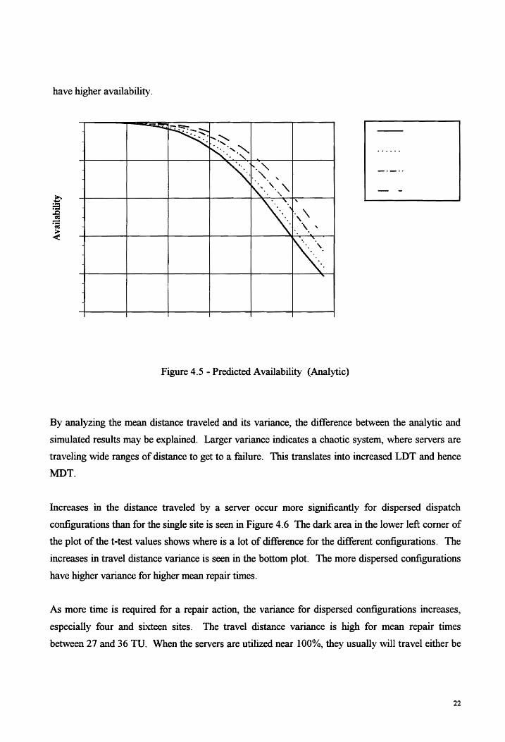
have higher availability.

Figure 4.5 - Predicted Availability (Analytic)

By analyzing the mean distance traveled and its variance, the difference between the analytic and

simulated results may be explained. Larger variance indicates a chaotic system, where servers are

traveling wide ranges of distance to get to a failure. This translates into increased LDT and hence

MDT.

Increases in the distance traveled by a server occur more significantly for dispersed dispatch

configurations than for the single site is seen in Figure 4.6 The dark area in the lower left comer of

the plot of the t-test values shows where is a lot of difference for the different configurations. The

increases in travel distance variance is seen in the bottom plot. The more dispersed configurations

have higher variance for higher mean repair times.

As more time is required for a repair action, the variance for dispersed configurations increases,

especially four and sixteen sites. The travel distance variance is high for mean repair times

between 27 and 36 TU. When the servers are utilized near 100%, they usually will travel either be

22

diverted on a return or travel directly from one repair action to another. This causes the differences

in the mean distance traveled to diminish. The mean travel time continues to increase pass 7 .5

lengths for all configurations. This translates into higher MDT and decreased availability. This is

part of the explanation why the experimental availability is lower than the predicted availability.

See Figure 4.7 Additionally, the large queue of failed components may invalidate the REPS

assumption of finite queuing.

Even though there is significant improvement for the MDT, when MTTR is 12 and 15 TUs, this

does not translate into a significant improvement in system availability. There is some very small

improvement, but it is not statistically significant.

There is some rough correspondence between the significant differences in Figures 4.6 and Figure

4. 7. As the distance the server is required to travel increases, so does the MDT.

As the MDT increases, a queue of waiting failures build-up. Servers proceed from one failure to

another without returning to their home dispatch site. This minimizes the effect of dispersal. The

reduced variance in the distance traveled is due to the fact that the servers in the one site

configuration head for a centralized point. Other configuration servers, especially for four and

sixteen sites, are traveling to points that are almost any point on the system.

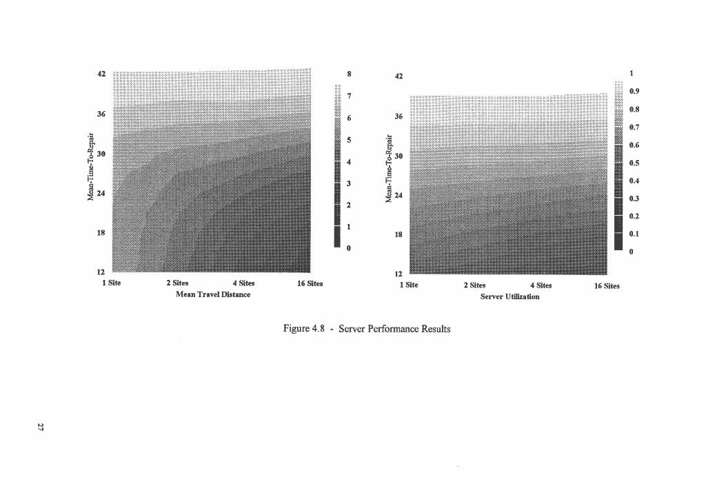
Comparing the server utilization rate against the mean distance travel, Figure 4.8, shows that as

the server utilization approaches 100%, the mean distance traveled by a server is the same for all

dispatch configurations. This is caused by servers traveling directly from one component to

another without attempting to return to the dispatch . site. At a steady state near 100% server

utilization, the different configurations have no effect.

The system MDT and MTBF had a very large variance for several data points. This precluded the

performance of any valid analysis of these parameters.

The data from the experiment supports the contention that disperse sites might have detrimental

effects on availability by increasing the MDT. The high variance means that some servers are

traveling long distances. The effect conjectured did occur on availability, although not to the

23

Mean Travel Distance 1 Site

8

= 0 2 Sites .i ""

;::::::: 7 II

l:.~ 6

= ~ 5 t.: = 4 Sites 0 u

4 3 2

16 Sites 1

12 18 24 30 36 42 0

Travel Distance t-test Values 1 Site

= 0 .i 2 Sites

"" = ~ t.: 4 Sites = 0 u

16 Sites

12 18 24 30 36 42

Travel Distance Variance 1 Site

0.3

= 2 Sites 0.25 0

"i "" 0.2 = ~

t.: = 4 Sites 0.15 0 u 0.1

16 Sites 0.05

12 18 24 30 36 42 0

Figure 4.6 - Travel Distance Output

24

magnitude expected. There is no difference in availability for dispersed dispatch sites. The

dispersed sites are predicted by analytic means to have improved availability. This did not occur.

4.2 Multiple Types of Distributions

A second experimental was run with different distributions. The repair time was sampled from an

Erlang distribution with a shape parameter of two. The time between failures distribution was

lognonnal with a variance of 200. The LDT sampling continued from an exponential distribution.

All means remained the same.

Figure 4.9 shows that the availability for both this case and the base case. For this case, the 80%

availability level is reached with a MTTR of 12, as opposed to 30 for the base case.

In this experiment, the availability decreases very rapidly to zero. (more than sixteen simultaneous

failed components) The variance of the repair and failure rates is very important to the system's

performance. The same mean has yielded dramatically different results.

Comparisons of the actual versus the simulation predictions show the effect of changing the

distributions. Figure 4.lOa/b The actual availability is rapidly decreasing, while the predict

decreases in an exponential shape curve. This comparison emphasizes the important of considering

the distribution and variance, in addition to the mean, when evaluating a systems parameters.

There are only two points that have significantly improvement in availability in a pair-wise

comparison against one dispatch site. These occurred for four and sixteen sites with a mean repair

time of 12 TU. Evaluation of smaller mean repair times would yield more significant changes in

availability. The low server utilization rate would allow the closes site to have a server ready to be

sent. The dispersal configurations would lower the mean travel distance , hence the LDT and

MDT.

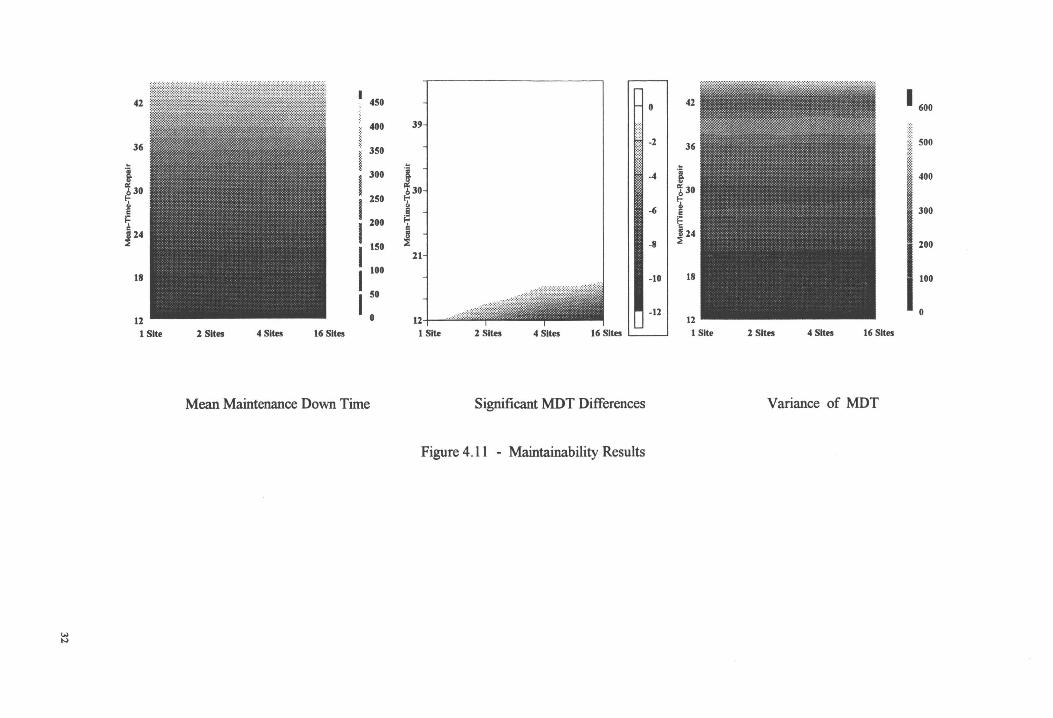
As the mean repair time grows above 24 TU, there are no significant improvements in component

MDT. Availability is in the 90-95% range. The variance in the data above a mean repair time of

18 makes analysis inconclusive. Figure 4.11

25

..., °'

42

36 .. ·;

i ~ 30 ~

~ ~ 24

~

18

12 1 Site 2 Sites 4 Sites 16 Sites

Configuration

MDT

Figure 4.7

.. 90

.11111

80

170 160

150

140 130 120 110

0

42

M 36 -~

i: ~ 30 I

I ..... E;4 24

~ :I

18

12~ 1 Site 2 Sites 4 Sites 16 Sites

Configuration

Significant Differences in MDT

t-test of MDT

Maintainability Results : Base Case

0

-5

-20

-25

-30

-35

-40

.... -.I

42

36

.!:l .. ~ 30 !";' .§ ~ ~ 24

18

12 1 Site 2 Sites 4 Sites

Mean Travel Distance

8 42 1

I : I'. r I 1

0

36

-~

~ 30 0

~ 8 f7 = ~ 24

18

I:: m 0.1

II I 0.6

I o.s

I 0.4

I 0.3

I 0.2

I 0.1

0

12 16 Sites 1 Site 2 Sites 4 Sites 16 Sites

Server Utilization

Figure 4.8 - Server Performance Results

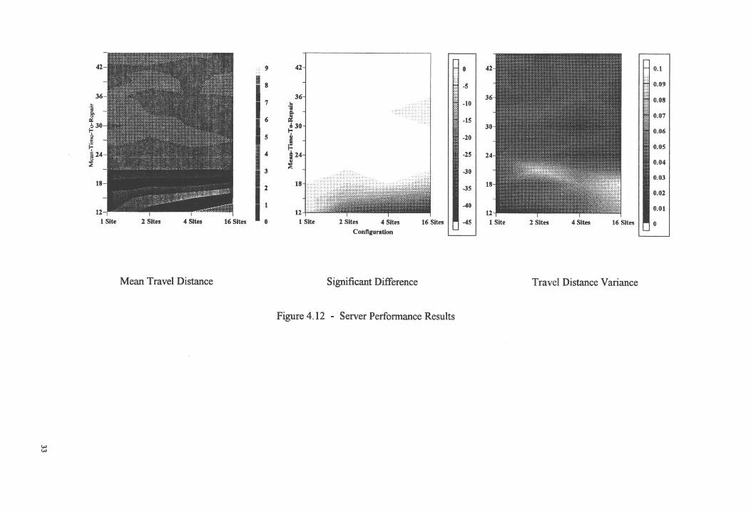
The mean travel distance levels off at 8 lengths for all configurations when the mean repair time is

greater than 21 TU. The variance is very small, implying a relatively ordered system, except for

16 dispatch sites configuration as shown in Figure 4.12. This could be a Type I error in the pair­

wise comparisons.

The main difference between this experiment and the base case is the mean repair time that the

availability decrease rapidly. The plots of the data were similar to the plot in the base case. The

experiment showed that the mean used to calculate a systems parameters does not take into account

the effects of different distributions on its performance.

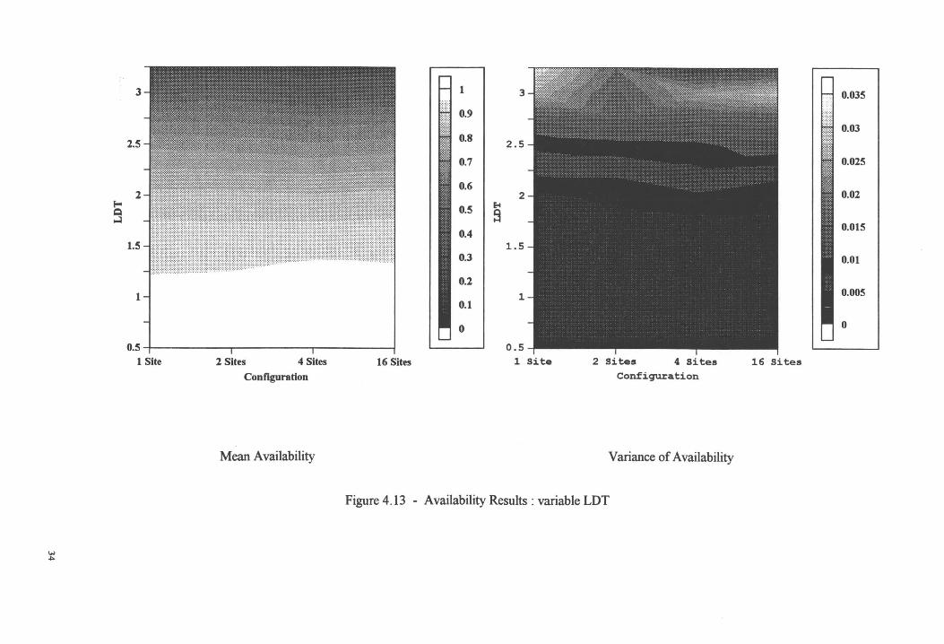
4.3 LDT Sensitivity Analysis

Sensitivity of the systems parameters to different LDT means was examined. The MTTR was set

at 24 TU and the LDT varied. The results in Figure 4.13 show that availability is not effected by

different configurations. The system's availability is sensitive to changes in the LDT.

The variance of the availability, in Figure 4.13, grows with increases in the mean LDT. For mean

LDT 2.0 TU/ length, the large variance reduces confidence in the results of the analysis. With an

a-level of 0. 05, there is only one point of significant improvement in availability. The point is a

four site configuration with mean LDT of 1.25.

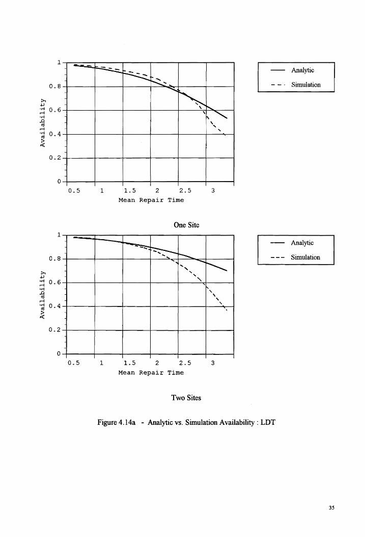
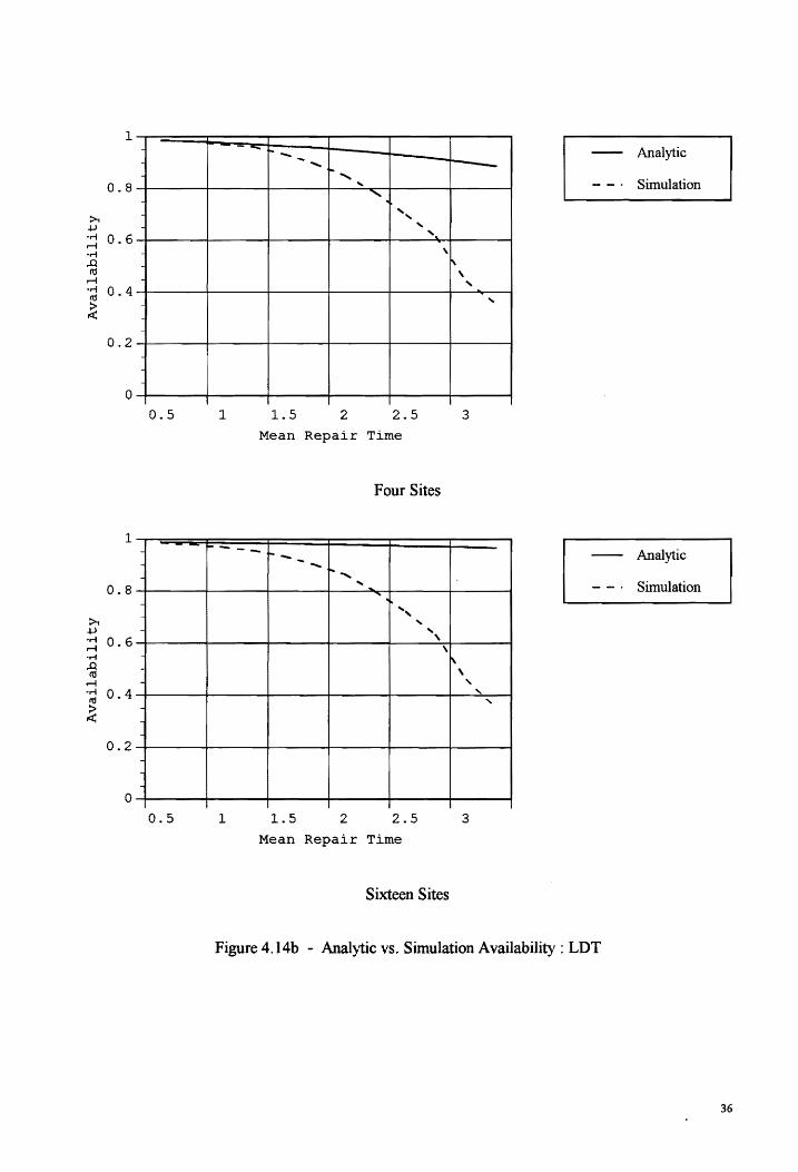
The actual availability is always less than the predicted. Its rate of decrease is greater also. The

predicted and experimental availability for a single centralized configuration showed some

correlation. The two site configuration, Figure 4.14a/b, also had some correlation, but to a lesser

extent.

The MDT was significantly better for the dispersed sites for mean LDT in the 0.5 to 1.5 range.

For larger values of LDT the significant differences drop-off, Figure 4 .15 This improvement in the

MDT for dispersed configurations does not translate into improved system availability because the

difference between the availabilities was small.

Comparison of the varying the repair time and the LDT showed little significant differences in

availability. The case where the mean LDT is varied, the availability decreases slower. This is

due to the smaller time increments used.

28

" o.8

o.6

Exponential Distribution

., .. ~ ~-- Jb ~~~

~

Erlang Repair Time I Lognormal Failure

0.8

0.6 . .c. :S ~

0.4 ,!! ·;; ~ ~

0.2

1

0.8

0.6 ~ :s 0.4 ~

~

0.2

Figure 4.9 - Base Case vs. Multiple Distribution Availability

29

1

0.8

>< +->

:::o.6 ...... ..Q !ti .-I

·;;o.4 ~

0.2

a

'

12

' "'\ \

\ \ \

\

\ \

18

--....... ~

\ ·~··

\

\

~

~ ~

~ \ ~ , .....

\ \ .... ... 24 30 36 42

Mean Repair Time

' \ .....

One Site

O-+-------+-------+--------+------+----~------(

12 18 24 30 36 42 Mean Repair Time

Two Sites

Figure 4. lOa - Availability Results : Multiple Distribution

Analytic

Simulation

Analytic

Simulation

30

:;... ..µ

1

0.8

;::o.6 -...; ..Q

1\1 ......;

·;t; 0.4 ~

0.2

0

1

0.8

:;... ..µ

::: 0.6 -...; ..Q a:!

......;

-~ o. 4 ~

0.2

0

' ' '

12

-I ' ' ' -j

-j

12

~ ~ \

\

Analytic

Simulation ~

~ ' \ \

.-

~ \ \

~ \ \ .

~ \ \ \

\ ~

I' \ \

"" ... 18 24 30 36 42

Mean Repair Time

Four Sites

---........ N \

\.

Analytic

Simulation ~

~ \ \ \ -'

\

~ \ \ \ .

\ \ \

\ -,.

r-\ \ "- ...

18 24 30 36 42 Mean Repair Time

Sixteen Sites

Figure 4 .1 Ob - Availability Results : Multiple Distribution

31

w ....

36

i "'30 ~ ~ f; c J24

18

12 1 Site

450

400

~ 350

i 300

I 250

I 200

I 150

I 100

50

0

2 Sites 4 Sites 16 Sites

Mean Maintenance Down Time

0

39 ::::

t -2

.. ;i -4

130

~ .§ -6 I-;' c

~ -8 21

-10

..... ;:::::::::~:!~t}{fj~~~~=~=~~~~~~l~~t~

12 I ..... :=·=:::;::::::=:g:;;;~p·r I I LJ -12

1 Site 2 Sites 4 Sites 16 Sites

Significant MDT Differences

Figure 4.11 - Maintainability Results

42 I 600

·::::

36 :I·, 500

l 1~ ~30 E 300 i: c ~24

r 18 100

0 12 1 Site 2 Sites 4 Sites 16 Sites

Variance of MDT

... ...

42

36-.. "ii -ft al: b30-

!;-~

E7 ii 24-l

18

12 1 Site

9

I : I:

3

I 2

I o I

2 Sites 4 Sites 16 Sites

Mean Travel Distance

42 0 I 42 I H 0.1

-5 I'" 36 36 0.08 .. -10 ·; D.

0.07 il! -15 ~30 30 I Ill 0.06

i -20

!= -251

11111 o.os ! 24 24

~ 1 • 0.04 -30

rm111fil';'=m::::.:::aw;twzuw~E::W:~ 1 • 0.03 18

-JS 18

;"':°/· .. '· '·.' I I 0.02 -40 ~i~J~ 0.01 12 ·.··.·.·:·:·:·:·:·:·:·'

16 Sites I ~ -4S

12 ".;;....

1 Site 2 Sites 4 Sites 1 Site 2 Sites 4 Sites 16 Sites I ri o Connguratlon

Significant Difference Travel Distance Variance

Figure 4.12 - Server Performance Results

w -"'

E-­~ .J

3 3

2.5 2.5

2 2

1.5 1.5

1 1

0.5 -+--------.---------.-------! 0.5 I

1 Site 2 Sites 4 Sites 16 Sites 1 Site 2 Sites 4 Sites

Configuration Configuration

Mean Availability Variance of Availability

Figure 4.13 - Availability Results: variable LDT

0.035

·:·:·:·

f1 0.03

iii~. 0.025

0.02

0.015

0.01

0.005

0

16 Sites

1 Analytic

0.8 Simulation

:;:..., .µ ·r-1 0.6 r-1 ·ri ..0

n:S ' ' r-1 ·r-i 0.4 ttt ' ~

0.2

0

0.5 1 1. 5 2 2.5 3

Mean Repair Time

One Site 1 ....__

0.8

:;:..., .µ ·r-1 0.6 r-1 ·rl ..0 n1

r-1 ·r-1 0.4 "' ~

-~ ~ ........ ~ """~ -.....

"' ... ' ' ' ' '" ' ' ' ' .....-,

Analytic

Simulation

-I

0.2 ., -I

-I

0

0.5 1 1.5 2 2.5 3

Mean Repair Time

Two Sites

Figure 4.14a - Analytic vs. Simulation Availability: LDT

35

1 -- ...... ""'- - Analytic

0.8 ' I-' ....

'~ Simulation

~ ,.µ ·r-1 0.6 ....; ·r-1 ..0

11:1

,, ' ~

' i' ' ....;

·r-1 0.4 «1

~ ' ........

'

0.2

0

0.5 1 1.5 2 2.5 3

Mean Repair Time

Four Sites

1

0.8

~

-1 ~--- t- -- .... _

-1 -..... ., "" ...... '..:!lo.

., ..... ~ I' .... ., ' '

Analytic

Simulation

.µ ·r-1 0.6 ....;

., ' \

' ·r-1 ..0 m

-

" 4 \ ....; 4 ' ·r-1 0.4 rd ' ' ~ 4

0.2 4

0

0.5 1 1.5 2 2.5 3

Mean Repair Time

Sixteen Sites

Figure 4.14b - Analytic vs. Simulation Availability: LDT

36

"' ...:a

~ Q ~

3

2.5

2

1.5

1

0.5 1 Site 2 Sites 4 Sites

Configuration

Mean MDT

70

60

40 §

30

20

10

0

16 Sites

3

2.5

2

1.5

0.5 ···.·.·.,.,,,,.,.,.,.

I Site 2 Sites 4 Sites

Configuration

Significant Differences in MDT

t-test

Figure 4.15 - Maintainability Results: variable LDT

f' . \ -2

. -3

-4

-5

-6

-7

-8

-9

16 Sites

V. SUMMARY AND CONCLUSIONS

An evaluation of the effect of repair server location on a system's availability was performed

using computer simulation. Four different configurations for the dispersal of the repair servers

were analyzed. The population of components requiring repair actions were distributed over a

large service area. Different time-to-repair and time-to-failure distributions were used.

Dispersal of server dispatch sites did not effect system availability, in either a positive or negative

manner. The hypothesis that there would be some decrease was not supported. The reason

explaining the absence of improvement in the availability is the variance. The higher variance for

the distance traveled by the servers in the dispe~se configurations indicates that some servers are

being sent far across the grid. This increases their total LDT and hence there MDT. This is why

the smaller mean distance for the dispersed cases did not induce improvements in the systems

availability.

For the range of values, the system was sensitive to changes in components of the MDT. This

sensitivity resulted whether the LDT or MTIR was varied. Under the conditions of this

experiment, dispersal played an insignificant role in effecting the availability.

Some of the cause for the increased MDT is that queues of failed components formed. They had to

wait for a server to finish, when the system had more than sixteen simultaneous failures.

This experiment is limited in its applications because of the many system variables that were held

constant. Further experiments that analyzed the systems sensitivity to the number of units that has

to fail before the system became unavailable would be insightful. The number of servers could be

varied also. The main reason that sixteen servers was select was to allow equal number of servers

at dispatch sites.

There are numerous restrictions that could be place on the servers actions. One is that a server

would have to return to a dispatch site after a given number of repair actions or time. The effects

of shutting down working components when the system was unavailable would be realistic for

many systems. Different means, depending on the direction traveling, could simulate the effects of

traffic flow. Servers could be susceptible to malfunctions.

38

The variety of data available from a simulation makes it a very valuable tool. It should be used to

refine preliminary designs of systems. It cannot replace analytic practice in system design. When

possible, analytic methods are preferred, however most real world systems are too complicated and

cannot be solved using solely analytic calculations. The reliance of most analytic methods on the

assumption of exponential behavior limits the number of situations that they may be successfully

used.

For a logistics support type system, the results of this project should be considered when deciding

on a maintenance concept Not only should costs and performance means be considered, the

effects on the variance of the factors needs to be analyzed when developing a system.

Future investigations into the effects of different input distributions should be performed.

Evaluation of a system's sensitivity to the variance of a distributions is inorder.

39

GENERAL REFERENCES

Grosh, Doris Lloyd, A Primer of Reliability Theory, 1st Edition, John Wiley and Sons, Inc., New York, NY, 1989

Hillier, Fredrick S., Lieberman, Gerald J., Introduction to Operations Research .5th Edition, McGraw Hill, Inc., New York, NY, 1990

Pritsker, A. Alan B., Sigal, C. Elliott, Hammesfahr, R.D. Jack, SLAM II : Network Models For Decision Support, Prentice-Hall, Inc., Englewood Cliffs, NJ, 1989

Pritsker, A. Alan B., Introduction to Simulation and SLAM II, 3rd Edition, Halsted Press Books, New York, NY, 1986

Warpole, Ronald E., Myers, Raymond H., Probability and Statistics for Engineers and Scientists, 4th Edition, Macmillan Publishing Company, New York, NY, 1989

40

APPENDIX

41

//LDI JOB 32769,WEISSMANN,TIME=60,REGION=4M /*PRIORITY IDLE /*ROUTE PRINT VTVMI.ISE154 /*JOBPARM LINES=99 //STEPl EXEC SLAMCG //FORT.SYSIN DD*

PROGRAM MAIN DIMENSION NSET{20000) COMMON/SCOMl/ATRIB(lOO),DD(IOO),DDL{lOO),D1NOW,II,

*MFA,MSTOP,NCLNR,NCRDR,NPRNT,NNRUN,NNSET,NTAPE, *SS(IOO),SSL(IOO),TNEXT,TNOW,XX(IOO) COMMON QSET(20000) EQUIV ALENCE(NSET{l),QSET{l)) NNSET=20000 NCRDR=5 NPRNT=6 NTAPE=7 CALL SLAM STOP END

SUBROUTINE EVENT(I) COMMON/SCOMl/ATRIB(lOO),DD(lOO),DDL(IOO},DTNOW,11,

*MFA,MSTOP,NCLNR,NCRDR,NPRNT,NNRUN,NNSET,NTAPE, *SS( I 00),SSL(l 00), TNEXT, TNOW,XX(l 00)

GO TO(l,2,3,4,5,6, 7 ,8),I

1 CALL FAIL URE RETURN

2 CALL REP ARED RETURN

3 CALLXMOVE RETURN

4 CALL YMOVE RETURN

5 CALL WORKERS RETURN

6 CALLPARTS RETURN

7 CALLCLEAN RETURN

8 CALLOPUT RETURN END

42

C************************************************************************* c C FAIL URE : ASSIGNS SERVER TO COMPONENT WHEN IT FAILS OR IF C NO SERVER IS AVAILABLE, PUTS COMPONENT IN A C WAITING FILE c C*************************************************************************

SUBROUTINE FAIL URE COMMON/SCOMI/ ATRIB(l 00),DD(l 00),DDL( 100),DTNOW,II,

*MFA,MSTOP,NCLNR,NCRDR,NPRNT,NNRUN,NNSET,NTAPE, *SS( I 00),SSL( 100), TNEXT, TNOW,XX(l 00) EQUIV ALEN CE (XX( 1O),ID),(XX(12),POSY) EQUIVALENCE (XX(13),POSX),{XX(l4),SERVER),(XX(l5),SUM) EQUIVALENCE (XX(l6),TSUM)

ATRIB(l)=TNOW CALL FILEM( l,ATRIB) ID=ATRIB(2) POSX=ATRIB(3) POSY=ATRIB( 4)

C SEARCHING FOR AVAILABLE SERVERS AT DISPATCH SITES

IF(NNQ(2).GT.O) THEN NEXT=MMFE(2) NTEMP=NEXT SUM= 100000.

10 IF(NEXT.EQ.O) GO TO 100 CALL COPY(-NEXT,2,ATRIB) TSUM=ABS(POSX-ATRIB(5))+ABS(POSY-ATRIB(6)) IF(TSUM.LT.SUM) THEN

NTEMP=NEXT SUM=TSUM

END IF NEXT=NSUCR(NEXT) GOTO 10

100 CALL RMOVE(-NTEMP,2,ATRIB) ATRIB(l)=TNOW ATRIB(2)=ID ATRIB(3)=POSX ATRIB(4}=POSY ATRIB(IO)=SUM CALL ENTER(l,ATRIB)

ELSE

43

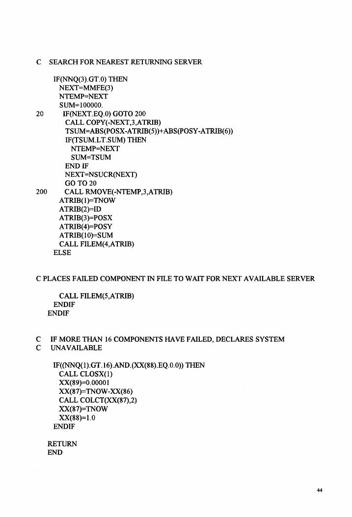
C SEARCH FOR NEAREST RETURNING SERVER

IF(NNQ(3).GT.O) THEN NEXT=MMFE(3) NTEMP=NEXT SUM=IOOOOO.

20 IF(NEXT.EQ.O) GOTO 200 CALL COPY(-NEXT,3,ATRIB) TSUM=ABS(POSX-ATRIB(5))+ABS(POSY-ATRIB(6)) IF(TSUM.LT.SUM) THEN

NTEMP=NEXT SUM=TSUM

END IF NEXT=NSUCR(NEXT) GOT020

200 CALL RMOVE(-NTEMP,3,ATRIB) ATRIB(l)=TNOW ATRIB(2)=ID ATRIB(3)=POSX ATRIB(4)=POSY ATRIB( I O)=SUM CALL FILEM(4,ATRIB)

ELSE

C PLACES FAILED COMPONENT IN FILE TOW AIT FOR NEXT AVAILABLE SERVER

CALL FILEM(5,ATRIB) END IF

ENDIF

C IF MORE THAN 16 COMPONENTS HAVE FAILED, DECLARES SYSTEM C UNAVAILABLE

IF((NNQ(l).GT.16).AND.(XX(88).EQ.O.O)) THEN CALL CLOSX(l) XX(89)=0.00001 XX(87)=TNOW-XX(86) CALL COLCT(XX(87),2) XX(87)=TNOW XX(88)=1.0

END IF

RETURN END

44

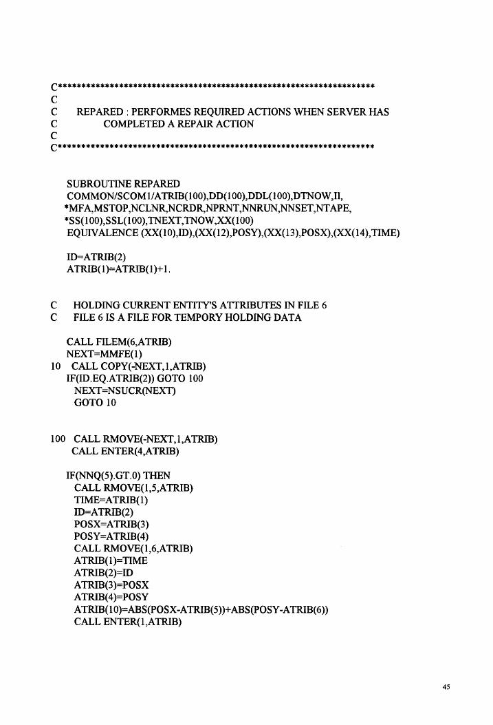
C******************************************************************** c C REPARED: PERFORMES REQUIRED ACTIONS WHEN SERVER HAS C COMPLETED A REP AIR ACTION c C********************************************************************

SUBROUTINE REP ARED COMMON/SCOMl/ATRIB(IOO),DD(lOO),DDL(IOO),DTNOW,II,

*MFA,MSTOP,NCLNR,NCRDR,NPRNT,NNRUN,NNSET,NTAPE, *SS(lOO),SSL(lOO),TNEXT,TNOW,XX(lOO) EQUIVALENCE (XX(IO),ID),(XX(l2),POSY),(XX(l3),POSX),(XX(l4),TIME)

ID=ATRIB(2) A TRIB( 1 )=A TRIB( I)+ 1.

C HOLDING CURRENT ENTITY'S ATTRIBUTES IN FILE 6 C FILE 6 IS A FILE FOR TEMPORY HOLDING DATA

CALL FILEM(6,ATRIB) NEXT=MMFE(l)

10 CALL COPY(-NEXT,1,ATRIB) IF(ID.EQ.ATRIB(2)) GOTO 100

NEXT=NSUCR(NEXT) GOTO 10

100 CALL RMOVE(-NEXT,l,ATRIB) CALL ENTER(4,ATRIB)

IF(NNQ(S).GT.O) THEN CALL RMOVE(l,5,ATRIB) TIME=ATRIB(l) ID=A TRIB(2) POSX=A TRIB(3) POSY=ATRIB(4) CALL RMOVE(l,6,ATRIB) A TRIB(l )=TIME A TRIB(2)=ID ATRIB(3)=POSX ATRIB(4)=POSY ATRIB(IO)=ABS(POSX-ATRIB(5))+ABS(POSY-ATRIB(6)) CALL ENTER(l,ATRIB)

45

ELSE CALL RMOVE{l,6,ATRIB) CALL FILEM(3,ATRIB) CALL ENTER(5,ATRIB)

END IF

C CHECKING TO SEE IF SYSTEM HAS MORE THAN 16 FAILED COMPONENTS

IF((NNQ(l).LE. l 6).AND.(XX(88).EQ. l .O))THEN CALL OPEN(l) XX(89)=1.0 XX(88)=0.0 XX(86)=TNOW-XX(87) CALL COLCT(XX(86),l) XX(86)=TNOW

END IF RETURN END

46

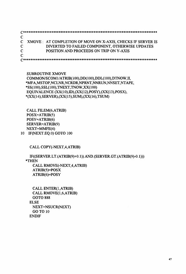
C**************************************************************************** c C XMOVE : AT COMPLETION OF MOVE ON X-AXIS, CHECKS IF SERVER IS C DIVERTED TO FAILED COMPONENT, OTHERWISE UPDATES C POSITION AND PROCEEDS ON TRIP ON Y-AXIS c C****************************************************************************

SUBROUTINE XMOVE COMMON/SCOMl/ATRIB(lOO),DD(lOO},DDL(lOO),DTNOW,II, *MF A,MSTOP ,NCLNR,NCRDR,NPRNT,NNRUN,NNSET,NT APE, *SS(lOO},SSL(lOO),TNEXT,TNOW,XX(lOO) EQUN ALENCE (XX(l0),ID),(XX(l2),POSY),(XX(13),POSX), *(XX(l4),SERVER),(XX(l5)'.tSUM},(XX(l6),TSUM)

CALL FILEM(6,ATRIB) POSX=ATRIB(5) POSY=ATRIB(6) SERVER=ATRIB(9) NEXT=MMFE(4)

10 IF(NEXT.EQ.O) GOTO 100

CALL COPY(-NEXT,4,ATRIB)

IF((SERVER.LT.(ATRIB(9)+0. l)).AND.(SERVER.GT.(ATRIB(9)-0. l))) *THEN

CALL RMOVE(-NEXT,4,A TRIB) ATRIB(5)=POSX ATRIB(6)=POSY

CALL ENTER(l,ATRIB) CALL RMOVE(l,6,ATRIB) GOTO 888

ELSE NEXT=NSUCR(NEXT) GOTO 10

END IF

47

100 NEXT=MMFE(3) 101 IF(NEXT.EQ.O) GOTO 770

CALL COPY(-NEXT,3,ATRIB) IF((SERVER.LT.(ATRIB(9)+0.l)).AND.(SERVER.GT.(ATRIB(9)-0.1)))

*THEN CALL RMOVE(-NEXT,3,ATRIB)

ELSE NEXT=NSUCR(NEXT) GOTO 101

END IF

770 CALL RMOVE(l,6,ATRIB) IF((A TRIB(6).LT.(A TRIB(8)+0. l )).AND.(ATRIB(6).GT.(ATRIB(8)-0. l))) *GOT0700

IF(A TRIB( 6).GT .(A TRIB(8)+0 .1)) A TRIB( 6)=A TRIB( 6)-1. 0 IF(A TRIB( 6).L T.(A TRIB(8)-0 .1)) A TRIB( 6)=ATRIB( 6)+ I. 0 CALL FILEM(3,ATRIB) CALL ENTER(3,ATRIB) GOTO 888

700 IF((A TRIB(5).LT.(A TRIB(7)+0.l)).AND.(ATRIB(5).GT.(A TRIB(7)-0. l))) *GOTO 701

IF(ATRIB(5).GT.(ATRIB(7)+0.l)) ATRIB(5)=ATRIB(5)-LO IF(A TRIB(5).LT .(A TRIB(7)-0. l)) ATRIB(5)=A TRIB(5)+ 1. 0 CALL FILEM(3,ATRIB) CALL ENTER(2,ATRIB) GOTO 888

701 CALL FILEM(2,A TRIB) 888 RETURN

END

48

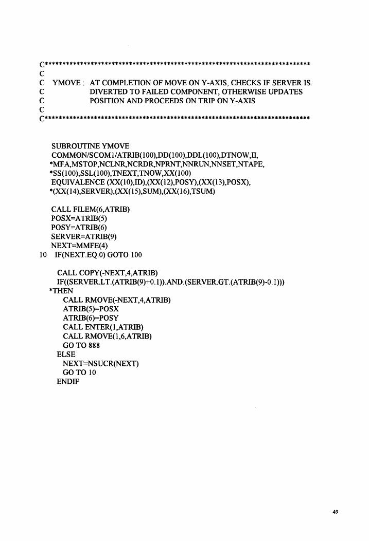
C**************************************************************************** c C YMOVE : AT COMPLETION OF MOVE ON Y-AXIS, CHECKS IF SERVER IS C DIVERTED TO FAILED COMPONENT, OTHERWISE UPDATES C POSITTON AND PROCEEDS ON TRIP ON Y-AXIS c C****************************************************************************

SUBROUTINE YMOVE COMMON/SCOMI/ ATRIB(l 00),DD( 100),DDL(l 00),DTNOW,II,

*MFA,MSTOP,NCLNR,NCRDR,NPRNT,NNRUN,NNSET,NTAPE, *SS(lOO),SSL(lOO},TNEXT,TNOW,XX(lOO) EQUIVALENCE (XX(l0),ID),(XX(l2),POSY),(XX(13),POSX), *(XX( 14},SERVER),(XX(15),SUM),(XX( 16), TSUM)

CALL FILEM( 6,ATRIB) POSX=ATRIB(5) POSY=ATRIB(6) SERVER=ATRIB(9) NEXT=MMFE(4)

10 IF(NEXT.EQ.O) GOTO 100

CALL COPY(-NEXT,4,ATRIB) IF((SERVER.LT.(ATRIB(9}+0. l)).AND.(SERVER.GT.(ATRIB(9)-0. l)))

*THEN CALL RMOVE(-NEXT,4,ATRIB) A TRIB(5)=POSX ATRIB(6)=POSY CALL ENTER(l,ATRIB) CALL RMOVE(l,6,ATRIB) GOTO 888

ELSE NEXT=NSUCR(NEXT) GOTO 10

END IF

49

100 NEXT=MMFE(3) 101 IF(NEXT.EQ.O) GO TO 999

CALL COPY(-NEXT,3,ATRIB)

IF((SERVER.LT.(A TRIB(9)+0. l)).AND.(SERVER.GT.(ATRIB(9)-0. l))) *THEN

CALL RMOVE(-NEXT,3,ATRIB) ELSE

NEXT=NSUCR(NEXT) GOTO 101

END IF

999 CALL RMOVE(l,6,ATRIB)

IF((A TRIB(5).L T.(A TRIB(7)+0 .1) ).AND. (ATRIB(5). GT .(A TRIB(7)-0 .1))) *GOTO 700

IF(ATRIB(5).GT.(ATRIB(7)+0. l)) ATRIB(5)=ATRIB(5)-l .O IF(ATRIB(5).LT.(ATRIB(7)-0.1)) ATRIB(5)=ATRIB(5)+ 1.0 CALL FILEM(3,A TRIB) CALL ENTER(2,ATRIB)

GOTO 888 700 IF((ATRIB(6).LT.(ATRIB(8)+0.l)).AND.(ATRIB(6).GT.(ATRIB(8)-0.l)))

*GOTO 701 IF(ATRIB( 6).GT .(A TRIB(8)+0. l)) ATRIB( 6)=ATRIB( 6)-1. 0 IF(A TRIB(6).LT.(A TRIB(8)-0. l)) ATRIB(6)=ATRIB(6)+ 1.0 CALL FILEM(3,ATRIB) CALL ENTER(3,ATRIB) GOTO 888

701 CALL FILEM(2,A TRIB)

888 RETURN END

50

C**************************************************************************** c C WORKERS : INITIALIZES ATTRIBUTES OF THE SERVERS c C****************************************************************************

SUBROUTINE WORKERS COMMON/SCOM 11ATRIB(l00),DD{l 00),DDL( 100),DTNOWJI, *MFA,MSTOP,NCLNR,NCRDR,NPRNT,NNRUN,NNSET,NTAPE, *SS( I 00),SSL(l 00), TNEXT, TNOW,XX( 100) ATRIB(9)=XX(6) XX(6)=XX(6)+ L ATRIB(5)=A TRIB(7) ATRIB( 6)=A TRIB(8) CALL FILEM(2,ATRIB) RETURN END

C**************************************************************************** c c c

PARTS- INITIALIZES ATI'RIBUTE VALUES FOR COMPONENTS

C****************************************************************************

SUBROl[TINE PARTS COMMON/SCOMl/ATRIB(IOO),DD(lOO),DDL(lOO),DTNOW,II,

*MFA,MSTOP,NCLNR,NCRDR,NPRNT,NNRUN,NNSET,NTAPE, *SS(IOO),SSL(IOO),TNEXT,TNOW,XX(IOO) A TRIB(2)=XX(5) IF(XX(3).GE.12.)THEN

XX(3)=0. XX(4)=XX(4)+ 1.

END IF XX(3)=XX(3)+ 1. A TRIB(3)=XX(3) ATRIB(4)=XX(4) XX(5)=XX(5)+ 1. RETURN END

SI

C**************************************************************************** c c c

CLEAN- CLEARS STATISTICAL ARRAYS WHEN CALLED BY NE1WORK

C****************************************************************************

SUBROUTINE CLEAN COMMON/SCOM 1/ A TRIB{l 00),DD( 100),DDL( 100),DTNOW,II,

*MFA,MSTOP,NCLNR,NCRDR,NPRNT,NNRUN,NNSET,NTAPE, *SS(lOO},SSL(lOO},TNEXT,TNOW,XX(lOO} CALL CLEAR RETURN END

C**************************************************************************** c c c

OPUT- WRITES DATA TO FILE FOR ANALYSIS

C****************************************************************************

c c c c c c c c c c

SUBROUTINE OPUT COMMON/SCOMl/ATRIB{lOO),DD(lOO),DDL(lOO),DTNOWJI, *MFA,MSTOP,NCLNR,NCRDR,NPRNT,NNRUN,NNSET,NTAPE, *SS(lOO),SSL(lOO),TNEXT,TNOW,XX(lOO) WRITE(88, lO)FF A WT(l ),FF A VG(2),CCAVG( 4),CCA VG(2),CCNUM( 6),CCNUM(5) *,CCAVG{l),GGOPN{l),CCAVG(3),FFAVG(l)

FFAWT(l)­CCAVG(4)­CCAVG(2)­CCAVG(2)­CCNUM(6)­CCNUM(5)­CCAVG(l)­GGOPN(l)­FFAVG(l)-

COMPONENT REPAIR TIME SERVER UTILIZATION DISTANCE TRAVELED BY SEVER TO COMPONENT AVERAGE WAIT IN FILE 2 NUMBER OF FAILURES GREATER THAN 16 TOTAL NUMBER OF COMPONENT FAILURES SYSTEMMTTR PERCENT TIME GATE OPEN, MEASURES AVAILABILITY TIME FOR SERVER TO TRAVEL FROM DISPATCH SITE OR DIVERSION POINT TO FAILED COMPONENT

10 FORMAT(2X,' ',10F8.2) RETURN END

//GO.SYSIN DD *

S2

; NETWORK GEN,WEISSMANN,PR, 1/1/1993, 12; LIMITS, 7, 10, 1000; ; INITIALIZING VALUES INTLC,XX(2)=0.,XX(3)=0.,XX:(4)= l .,XX(5)= l .,XX(6)= l .,XX(89)= l .,XX(88)=0.; INTLC,XX( 50)=0 .5,XX(86)=0. O;

SEEDS,7111111(1),7222222(2),7333333(3); INITIALIZE,, 125000;

;INITIAL VALVES FOR RANDOM VARIABLES ; THESE WERE ALTERED FOR DIFFERENT CASES EQUIV ALENCE/EXPON(XX(50),2),LDT; EQUIV ALENCE/EXPON(400, 1 ),MTBF/EXPON(9,3),REP AIRING;

EQUIV ALENCE/XX(98),MTTR/30,MAINT; STAT,l,SYS MTTR; STAT,2,SYS MTBF; NETWORK;

GATE/AVAILABLE,OPEN,7;

; CREATES THE COMPONENT ENTITIES CREATE,0,0,1,144,1; EVENT,6,1; ACTMTY,ATRIB(l);

BREA EVENT,1,1; TERMINATE;

'

ENTER,4,1; ACTIVITY,MTBF,,BREA; ACT,,,BREA;

GBAK ENTER,2,1; ACTIVITY,LDT;

ZAAC EVENT,3; TERMINATE; ENTER,5,1; ACT,,,ZAAC;

ENTER,3,1; ACTM1Y,LDT;

ZAAE EVENT,4; TERMINATE;

53

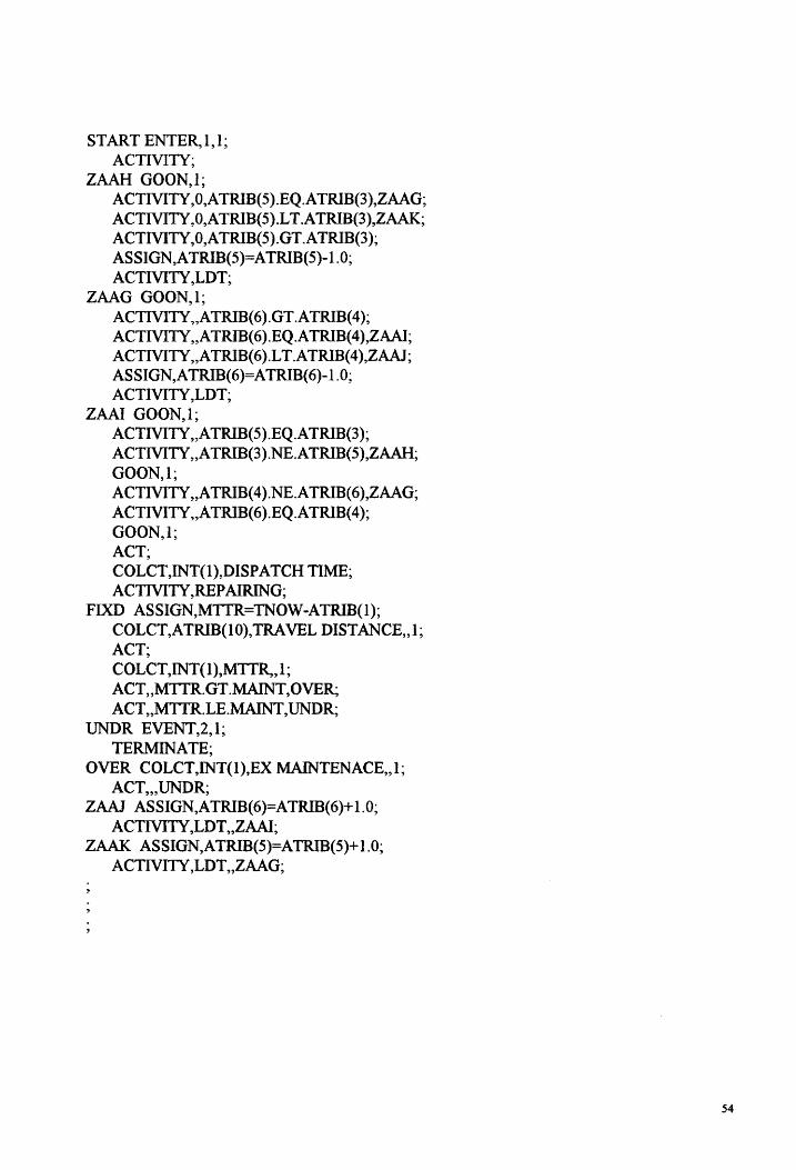
START ENTER,1,1; ACTIVITY;

ZAAH GOON,l; ACTIVITY,O,ATRIB(5).EQ.ATRIB(3),ZAAG; ACTIVITY,O,A TRIB(5).L T.ATRIB(3},ZAAK; ACTMTY,O,ATRIB(5).GT.ATRIB(3); ASSIGN,ATRIB(5)=A TRIB(5)-l .O; ACTIVITY,LDT;

ZAAG GOON,l; ACTIVITY,,A TRIB(6).GT.A TRIB( 4); ACTMTY,,ATRIB(6).EQ.ATRIB(4),ZAAI; ACTMTY,,A TRIB(6).LT.A TRIB( 4),ZAAJ; ASSIGN ,A TRIB( 6)=ATRIB( 6)-1. 0; ACTIVITY,LDT;

ZAAI GOON,l; ACTMTY,,ATRIB(5).EQ.ATRIB(3); ACTIVITY,,ATRIB(3).NE.ATRIB(5),ZAAH; GOON,l; ACTIVITY,,A TRIB( 4).NE.A TRIB(6),ZAAG; ACTMTYnATRIB(6).EQ.ATRIB(4); GOON,l; ACT; COLCT,INT(l),DISPATCH TIME; ACTMTY,REPAIRING;

FIXD ASSIGN,MTTR=TNOW-ATRIB(l); COLCT,ATRIB(lO),TRA VEL DISTANCE,,1; ACT; COLCT,INT( I ),MITR,, l; ACT,,MTTR.GT.MAINT,OVER; ACT,,MTTR.LE.MAINT,UNDR;

UNDR EVENT,2,1; TERMINATE;

OVER COLCT,INT(l),EX MAINTENACE,,l; ACT,,, UNDR;

ZAAJ ASSIGN,ATRIB(6)=ATRIB(6)+ 1.0; ACTMTY,LDT,,ZAAI;

ZAAK ASSIGN,ATRIB(5)=ATRIB(5)+ 1.0; ACTIVITY,LDT,,ZAAG;

54

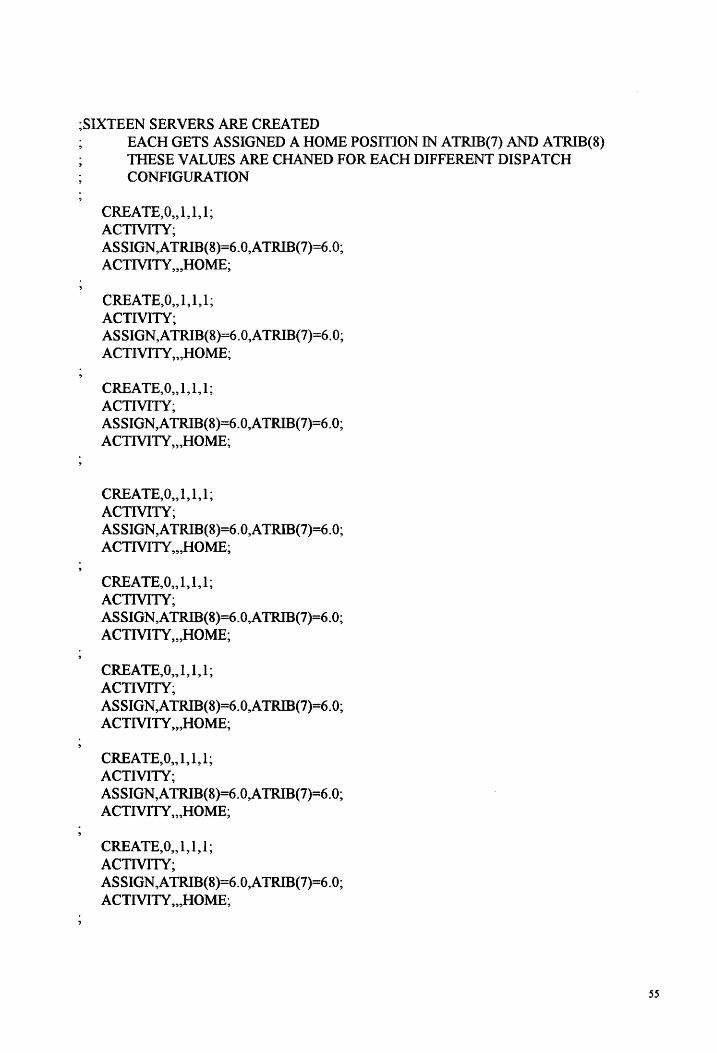
;SIXTEEN SERVERS ARE CREATED EACH GETS ASSIGNED A HOME POSITION IN ATRIB(7) AND ATRIB(8) THESE VALVES ARE CRANED FOR EACH DIFFERENT DISPATCH CONFIGURATION

CREA TE,O,, 1, 1, I; ACTMTY; ASSIGN,ATRIB(8)=6.0,A TRIB(7)=6.0; ACTMTY,,,HOME;

CREATE,0,,1,1,1; ACTMTY; ASSIGN,ATRIB(8)=6.0,ATRIB(7)=6.0; ACTIVITY,,,HOME;

CREA TE, 0,, 1, 1, 1; ACTIVITY; ASSIGN,A TRIB(8)=6.0,ATRIB(7)=6.0; ACTIVITY,,,HOME;

CREATE,O,,l,1,1; ACTIVITY; ASSIGN,ATRIB(8)=6.0,ATRIB(7)=6.0; ACTIVITY,,,HOME;

CREATE,0,,1,1,1; ACTIVITY; ASSIGN,ATRIB(8)=6.0,ATRIB(7)=6.0; ACTMTY,,,HOME;

CREATE,0,,,1,1,1; ACTIVITY; ASSIGN,ATRIB(8)=6.0,ATRIB(7)=6.0; ACTMTY,,,HOME;

CREATE,0,,1,1,1; ACTIVITY; ASSIGN,A TRIB(8)=6.0,A TRIB(7)=6.0; ACTIVITY,,,HOME;

CREA TE, 0,, 1, 1, 1; ACTIVITY; ASSIGN,ATRIB(8)=6.0,ATRIB(7)=6.0; ACTMTY,,,HOME;

SS

CREATE,0,,1,1,1; ACTIVITY; ASSIGN,ATRIB(8}=6.0,ATRIB(7)=6.0; ACTIVITY,,,HOME;

CREATE,0,,1,tl; ACTMTY; ASSIGN,ATRIB(8)=6.0,A TRIB{7)=6.0; ACTMTY,,,HOME;

CREA TE, 0,, 1, 1, I; ACTMTY; ASSIGN,ATRIB(8)=6.0,ATRIB(7)=6.0; ACTIVITY,,,HOME;

CREATE,0,,1,1,1; ACTIVITY; ASSIGN,A TRIB(8)=6.0,A TRIB(7)=6.0; ACTMTY,,,HOME;

CREATE,0,,1,1,1; ACTIVITY; ASSIGN,ATRIB(8)=6.0,ATRIB(7}=6.0; ACTIVITY,,,HOME;

CREATE,O,,l,l,l; ACTIVITY; ASSIGN,ATRIB(8}=6.0,ATRIB(7)=6.0; ACTIVITY,,,HOME;

CREATE,0,,1,1,1; ACTIVITY; ASSIGN,ATRIB(8)=6.0,ATRIB(7)=6.0; ACTIVITY,,,HOME;

CREATE,0,,1,1,1; ACTIVITY; ASSIGN ,A TRIB(8)=6. O,A TRIB(7)=6. O; ACTMTY,,,HOME;

HOME EVENT,5~J; TERMINATE;

S6

TRIGGERS STATISTICS SAMPLING DATA TO OUTPUT FILE EVERY 5000 TIME UNITS

CREA TE,5000,5000,,, I; ACT; EVENT,8,1 ACT; TERM;

TRIGGERS CLEARING OF ST A TISTICS ARRAYS 2500 TIME UNITS AFTER START OF EACH RUN

CREA TE,5000,2500,,,1; ACT;

MANI EVENT, 7, 1 ACT; AW AIT(7),A V AILABLE,, I ACT; TERM; END NETWORK;

EACH SIMULA TE STATEMENT INCREMENTS EITHER LDT OR REP AIR TIME THIS PROGRAM SHOWS INCREMENTING LDT TO INCREMENT REP AIR TIME INSTEAD OF LDT, USE XX(50) IN REP AIRING RANDOM VARIABLE INSTEAD OF LDT RANDOM VARIABLE

SIMULATE; SEEDS, 7111111(1),7222222(2), 7333333(3); INTLC,XX(50)=0. 75;

' SIMULATE; SEEDS,7111111(1),7222222(2),7333333(3); INTLC,XX(50)=1.0;

' SIMULATE; SEEDS, 7111111(1),7222222(2),7333333(3); INTLC,XX(50)= 1.25;

' SIMULATE; SEEDS,7111111(1),7222222(2),7333333(3); INTLC,XX(50)=1.5;

' SIMULATE; SEEDS, 7111111(1), 7222222(2), 7333333(3);

57

INTLC,XX{50)=1.75;

' SIMULATE; SEEDS,7111111(1),7222222(2),7333333(3); INTLC,XX(50)=2. O;

' SIMULATE; SEEDS,7111111(1),7222222(2),7333333(3); INTLC,XX(50)=2.25;

' SIMULATE; SEEDS,7111111(1),7222222(2),7333333(3); INTLC,XX(50)=2.5;

' SIMULATE; SEEDS,7111111(1),7222222(2),7333333(3); INTLC,XX(50)=2. 75;

' SIMULATE; SEEDS,7111111(1),7222222(2),7333333(3); INTLC,XX(50)=3.0;

' SIMULATE; SEEDS,7111111(1),7222222(2),7333333(3); INTLC,XX(50)=3.25;

' FIN; l/FT88FOO 1 DD SYSOUT=C,DCB=LRECL= 123 /* II

58