Assessment of surface winds over the Atlantic, Indian, and Pacific Ocean sectors of the Southern Ocean in CMIP5 models: historical bias, forcing response, and state dependence

Assessment of surface winds over the Atlantic, Indian, and PacificOcean sectors of the Southern Ocean in CMIP5 models: historicalbias, forcing response, and state dependence

Thomas J. Bracegirdle,1 Emily Shuckburgh,1 Jean-Baptiste Sallee,1 Zhaomin Wang,2

Andrew J. S. Meijers,1 Nicolas Bruneau,1 Tony Phillips,1 and Laura J. Wilcox3

Received 13 July 2012; revised 20 December 2012; accepted 27 December 2012; published 30 January 2013.

[1] An assessment of the fifth Coupled Models Intercomparison Project (CMIP5) models’simulation of the near-surface westerly wind jet position and strength over the Atlantic,Indian and Pacific sectors of the Southern Ocean is presented. Compared with reanalysisclimatologies there is an equatorward bias of 3.3� (inter-model standard deviationof� 1.9�) in the ensemble mean position of the zonal mean jet. The ensemble meanstrength is biased slightly too weak, with the largest biases over the Pacific sector(�1.4� 1.2m/s, �19%). An analysis of atmosphere-only (AMIP) experiments indicatesthat 28% of the zonal mean position bias comes from coupling of the ocean/ice models tothe atmosphere. The response to future emissions scenarios (RCP4.5 and RCP8.5) ischaracterized by two phases: (i) the period of most rapid ozone recovery (2000–2049)during which there is insignificant change in summer; and (ii) the period 2050–2098 duringwhich RCP4.5 simulations show no significant change but RCP8.5 simulations showpoleward shifts (0.33, 0.18 and 0.27�/decade over the Atlantic, Indian and Pacific sectors,respectively), and increases in strength (0.07, 0.08 and 0.15m/s/decade, respectively). Themodels with larger equatorward position biases generally show larger poleward shifts (i.e.state dependence). This inter-model relationship is strongest over the Pacific sector(r=�0.91) and weakest over the Atlantic sector (r=�0.39). An assessment of jet structureshows that over the Atlantic sector jet shift is not clearly linked to indices of jet structurewhereas over the Pacific sector the distance between the sub-polar and sub-tropicalwesterly jets appears to be important.

Citation: Bracegirdle, T. J., E. Shuckburgh, J.-B. Sallee, Z. Wang, A. J. S. Meijers, N. Bruneau, T. Phillips, and L. J. Wilcox(2013), Assessment of surface winds over the Atlantic, Indian, and Pacific Ocean sectors of the SouthernOcean in CMIP5models:historical bias, forcing response, and state dependence, J. Geophys. Res. Atmos., 118, 547–562, doi:10.1002/jgrd.50153.

1. Introduction

[2] In recent decades, the climatological maximum innear-surface (10m) westerly winds over SouthernHemisphere mid latitudes (referred to hereinafter as the ‘sur-face jet’) has shifted polewards and strengthened. Currentmodelling and observational evidence suggests that this islargely in response to the depletion of stratospheric ozonewith an additional contribution from greenhouse gas(GHG) concentration increases [Thompson and Solomon,2002; Shindell and Schmidt, 2004; Arblaster and Meehl,2006; Roscoe and Haigh, 2007; Yang et al., 2007]. In theocean, the influence of these atmospheric changes has beenlinked to changes in sea ice, eddy kinetic energy, sea surface

temperature (SST), mixed-layer depth and circulation [Halland Visbeck, 2002; Meredith and Hogg, 2006; Sen Guptaand England, 2006; Verdy et al., 2006; Ciasto andThompson, 2008; Sallee et al., 2008, 2010; Stammerjohnet al., 2008; Thompson et al., 2011; Wang et al., 2011]. Inaddition, changes in the upper ocean associated with windforcing may have had an impact on carbon uptake andstorage in the Southern Ocean, both directly, throughupwelling and outgassing [e.g. Le Quere et al., 2007] and in-directly, by influencing nutrient cycles and phytoplanktonactivity [Lovenduski and Gruber, 2005; Lovenduski et al.,2007; Sallee et al., 2010]. An accurate representation ofthe surface westerly winds at southern mid-latitudes is there-fore critical to many aspects of the coupled climate system.[3] In terms of future projections, most of the recent and

current generation of climate models exhibit a poleward shiftand strengthening of the Southern Hemisphere surface jet inresponse to greenhouse gas (GHG) increases [Fyfe andSaenko, 2006; Miller et al., 2006; Bracegirdle et al., 2008;Wilcox et al., 2013]. However, model studies including pro-jected future ozone recovery have indicated that in australsummer (DJF) the response of the surface jet to GHG

1British Antarctic Survey, UK.2School of Marine Sciences, Nanjing University of Information Science

and Technology, China.3NCAS-Climate, Department of Meteorology, University of Reading, UK.

Corresponding author: Thomas J Bracegirdle, British Antarctic Survey,High Cross, Madingley Road, Cambridge, CB3 0ET. ([email protected])

©2013. American Geophysical Union. All Rights Reserved.2169-897X/13/10.1002/jgrd.50153

547

JOURNAL OF GEOPHYSICAL RESEARCH: ATMOSPHERES, VOL. 118, 547–562, doi:10.1002/jgrd.50153, 2013

increases may be largely cancelled out by the response toozone recovery during the first half of the 21st century[Miller et al., 2006; Son et al., 2010; Arblaster et al.,2011; Polvani et al., 2011]. A key advance of the climatemodels contributing to the recently compiled CoupledModel Intercomparison Project phase 5 (CMIP5) dataset[Taylor et al., 2012] is the universal inclusion of the repre-sentation of stratospheric ozone changes, which was omittedfrom some of the CMIP3 models. In addition, most of theCMIP3 models did not have a well-resolved stratosphere[Karpechko et al., 2008], whereas the CMIP5 ensembleincludes a number of so-called “high top” models with anupper boundary at or above 1 hPa. In addition, 12 of theCMIP5 models have a latitudinal grid spacing in the atmo-sphere of 1.5� or less (see Table 1) compared with onlytwo of the CMIP3 models [Maloney and Chelton, 2006];increased latitudinal resolution has been linked in somemodelling studies to reductions in the climatological posi-tion bias of the surface jet [Guemas and Codron, 2011;Hourdin et al., 2012]. These three developments make theCMIP5 ensemble of models more suitable than earliergenerations for assessing the response of the SouthernHemisphere jet to future climate change scenarios.[4] The focus of this study is on the projections of surface

winds, for which variations in present-day climatology andprojected change are of great importance in understanding

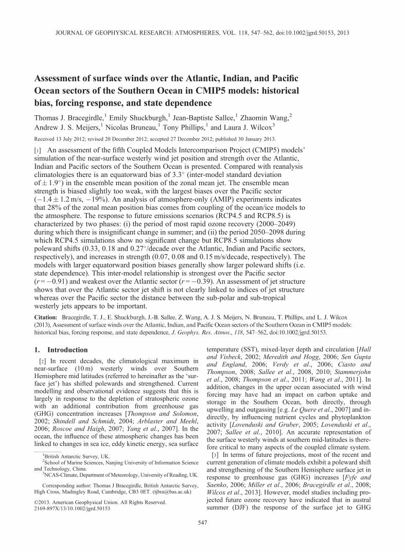
impacts on, and interactions with, the ocean. While a num-ber of studies have focussed on the response of zonal meantropospheric winds in coupled climate models [e.g. Wilcoxet al., 2013], here we assess the Atlantic, Indian and Pacificsectors individually. We are motivated to do this for tworeasons. The first is that it is important to understand thelongitudinal differences to assess the impact of the surfacewinds on the ocean, and in particular on carbon uptake[Sallee et al., 2010]. The second is that different mechan-isms may contribute to changes in the surface jet in differentsectors. For example, the atmospheric wave breaking char-acteristics vary zonally [Wang and Magnusdottir, 2011;Barnes and Hartmann, 2012], which is in part aconsequence of the longitudinal variations in orography as-sociated with South America and South Africa [Inatsu andHoskins, 2004]. From a storm-track perspective, a majorcyclogenesis region over the orography of South Americatriggers baroclinic eddies that follow a spiral track aroundthe whole Southern Ocean towards Antarctica in the Pacificsector [Hoskins and Hodges, 2005]. A secondary smallergenesis region over Australia and New Zealand feeds intothe Pacific storm track. This is partially reflected in thetime-mean westerly wind field, which shows a maximumat lower latitudes in the Pacific compared to the Atlantic(Figure 1). These zonal asymmetries in the storm track aremuch more pronounced in winter and are thought to be

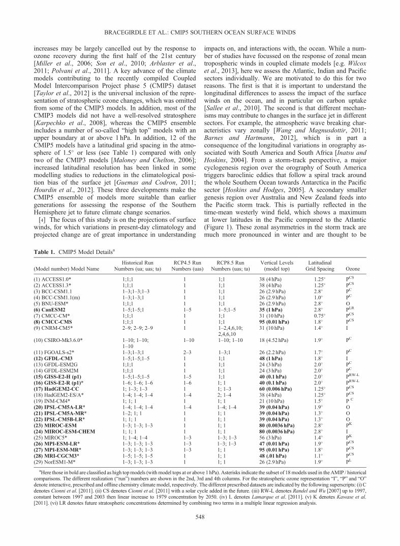
Table 1. CMIP5 Model Detailsa

(Model number) Model NameHistorical Run

Numbers (ua; uas; ta)RCP4.5 RunNumbers (uas)

RCP8.5 RunNumbers (uas; ta)

Vertical Levels(model top)

LatitudinalGrid Spacing Ozone

(1) ACCESS1.0* 1;1;1 1 1;1 38 (4 hPa) 1.25� PCS

(2) ACCESS1.3* 1;1;1 1 1;1 38 (4 hPa) 1.25� PCS

(3) BCC-CSM1.1 1–3;1–3;1–3 1 1;1 26 (2.9 hPa) 2.8� PC

(4) BCC-CSM1.1(m) 1–3;1–3;1 1 1;1 26 (2.9 hPa) 1.0� PC

(5) BNU-ESM* 1;1;1 1 1;1 26 (2.9 hPa) 2.8� O(6) CanESM2 1–5;1–5;1 1–5 1–5;1–5 35 (1 hPa) 2.8� PLR

(7) CMCC-CM* 1;1;1 1 1;1 31 (10 hPa) 0.75� PCS

(8) CMCC-CMS 1;1;1 1 1;1 95 (0.01 hPa) 1.8� PCS

(9) CNRM-CM5* 2–9; 2–9; 2–9 1 1–2,4,6,10; 31 (10 hPa) 1.4� I2,4,6,10

(10) CSIRO-Mk3.6.0* 1–10; 1–10; 1–10 1–10; 1–10 18 (4.52 hPa) 1.9� PC

1–10(11) FGOALS-s2* 1–3;1–3;1 2–3 1–3;1 26 (2.2 hPa) 1.7� PC

(12) GFDL-CM3 1–5;1–5;1–5 1 1;1 48 (1 hPa) 1.8� I(13) GFDL-ESM2G 1;1;1 1 1;1 24 (3 hPa) 2.0� PC

(14) GFDL-ESM2M 1;1;1 1 1;1 24 (3 hPa) 2.0� PC

(15) GISS-E2-H (p1) 1–5;1–5;1–5 1–5 1;1 40 (0.1 hPa) 2.0� PRW-L

(16) GISS-E2-R (p1)* 1–6; 1–6; 1–6 1–6 1; 1 40 (0.1 hPa) 2.0� PRW-L

(17) HadGEM2-CC 1; 1–3; 1–3 1 1; 1–3 60 (0.006 hPa) 1.25� PCS

(18) HadGEM2-ES/A* 1–4; 1–4; 1–4 1–4 2; 1–4 38 (4 hPa) 1.25� PCS

(19) INM-CM4* 1; 1; 1 1 1; 1 21 (10 hPa) 1.5� P C

(20) IPSL-CM5A-LR* 1–4; 1–4; 1–4 1–4 1–4; 1–4 39 (0.04 hPa) 1.9� O(21) IPSL-CM5A-MR* 1–2; 1; 1 1 1; 1 39 (0.04 hPa) 1.3� O(22) IPSL-CM5B-LR* 1; 1; 1 1 1; 1 39 (0.04 hPa) 1.3� O(23) MIROC-ESM 1–3; 1–3; 1–3 1 1; 1 80 (0.0036 hPa) 2.8� PK

(24) MIROC-ESM-CHEM 1; 1; 1 1 1; 1 80 (0.0036 hPa) 2.8� I(25) MIROC5* 1; 1–4; 1–4 1–3 1–3; 1–3 56 (3 hPa) 1.4� PK

(26) MPI-ESM-LR* 1–3; 1–3; 1–3 1–3 1–3; 1–3 47 (0.01 hPa) 1.9� PCS

(27) MPI-ESM-MR* 1–3; 1–3; 1–3 1–3 1; 1 95 (0.01 hPa) 1.8� PCS

(28) MRI-CGCM3* 1–5; 1–5; 1–5 1 1; 1 48 (.01 hPa) 1.1� PCS

(29) NorESM1-M* 1–3; 1–3; 1–3 1 1; 1 26 (2.9 hPa) 1.9� PL

aHere those in bold are classified as high topmodels (with model tops at or above 1 hPa). Asterisks indicate the subset of 18models used in theAMIP / historicalcomparisons. The different realization (“run”) numbers are shown in the 2nd, 3rd and 4th columns. For the stratospheric ozone representation “I”, “P” and “O”denote interactive, prescribed and offline chemistry climate model, respectively. The different prescribed datasets are indicated by the following superscripts: (i) Cdenotes Cionni et al. [2011]. (ii) CS denotes Cionni et al. [2011] with a solar cycle added in the future. (iii) RW-L denotes Randel and Wu [2007] up to 1997,constant between 1997 and 2003 then linear increase to 1979 concentration by 2050. (iv) L denotes Lamarque et al. [2011]. (v) K denotes Kawase et al.[2011]. (vi) LR denotes future stratospheric concentrations determined by combining two terms in a multiple linear regression analysis.

BRACEGIRDLE ET AL.: CMIP5 SOUTHERN OCEAN SURFACE WINDS

548

caused in part by asymmetries in tropical SSTs and conse-quent forcing [Inatsu and Hoskins, 2004]. Local forcing isalso a major contributor to zonal asymmetries, for examplethe maximum in time mean zonal wind over the Indiansector (see Figure 1) is largely caused by a local maximumin the pole-to-equator SST gradient [Inatsu and Hoskins,2004; Hoskins and Hodges, 2005].[5] In this study we assess present-day skill and projected

changes simulated by the CMIP5 models. As part of this as-sessment we address the question of whether the skill andprojected changes in models with a good representation ofthe stratosphere differs from those with a relatively poorlyresolved stratosphere. We also examine whether there is a‘state dependence’ in the model responses, following a num-ber of recent studies which have found that climate modelswith a larger poleward shift in response to GHG increasesgenerally exhibit a larger equatorward bias in their present-day mean state [Kidston and Gerber, 2010; Son et al.,2010]. In particular the theoretical implications of differ-ences in state dependence characteristics across differentocean sectors are investigated.[6] This paper is structured as follows. In the next section

(Section 2) the model and reanalysis datasets are described.In Section 3 the results are presented followed by discussionand conclusions in Section 4.

2. CMIP5 Model Data and Jet Diagnostics

[7] Data from the CMIP5 models were assessed in thisstudy. Throughout this study we quote the inter-modelspread of the results, however we note that some of themodels included in the study are very similar (e.g. theIPSL-CM5A-LR and IPSL-CM5A-MR models differ pre-dominantly only in their horizontal grid). The requiredvariables were downloaded from the CMIP5 data archive.These are: westerly wind on pressure levels (“ua”), 10-metrewesterly wind (“uas”) and temperature on pressure levels(“ta”). The CMIP5 simulations and forcing scenarios used

are shown in Table 1. In general more than one realization isavailable for a given model and a given scenario (i.e. the samemodel is run more than once with the same forcing). Wheremore than one realization is available (indicated in Table 1),the mean of those realizations is used. Before analysis the cli-mate model and reanalysis data were bi-linearly interpolatedonto the HadGEM2-ES horizontal grid (1.875� longitude1.25� latitude) to allow direct comparison.[8] The jet strength is defined as the climatological maxi-

mum in the zonal mean 10m westerly wind component inthe Southern Hemisphere and the jet position is defined asthe latitude of this maximum. A cubic spline interpolationis used to quantify the maximum and determine its latitudefrom the gridded data. In addition to zonal mean diagnostics,ocean sectors are assessed separately. The sectors aredefined by longitude ranges as follows: Atlantic sector(290�–20�), Indian sector (20�–150�) and Pacific sector(150�–290�), which are indicated in Figure 1.[9] For comparisons to reanalysis datasets, data from the

“historical” forcing simulations were used. The historicalsimulations are fully coupled experiments that are forcedby observed 20th century variations of important climatedrivers such as GHGs, ozone, aerosols and solar variability.For assessments of future change, two scenarios wereassessed: Representative Concentration Pathway (RCP) 4.5and RCP 8.5, for which the numbers refer to approximateestimates of radiative forcing at the year 2100. RCP4.5 is amedium mitigation scenario and RCP8.5 is a high emissionsscenario. A full range of anthropogenic climate drivers areincluded in the RCP scenarios (GHGs, aerosols, chemicallyactive gases and land use) along with a repeating 11-yearsolar cycle (repeating solar cycle 23), which are detailed inMeinshausen et al. [2011]. Recommended pathways forboth concentration and emissions of GHGs are provided,since both atmosphere-ocean general circulation modelsand Earth system models (ESMs) are included in CMIP5.[10] The CMIP5 models assessed here include representa-

tions of stratospheric ozone changes across both the histori-cal and RCP scenarios. However, only seven follow therecommended time series of Cionni et al. [2011] and theothers are based on a range of different methods anddatasets, which are listed in Table 1. Wilcox et al. [2013,submitted to JGR-Atmospheres] show that the ozoneconcentrations above Antarctica qualitatively follow thechanges seen in the Cionni et al. [2011] time series, but witha relatively large spread in absolute concentrations anddifferences in the rate of 21st century recovery.[11] The observationally constrained European Centre for

Medium Range Weather Forecasts (ECMWF) ERA-Interimreanalysis dataset [Dee et al., 2011] was used to assess theskill of the models at reproducing present-day climate.Recent studies have found ERA-Interim to be the mostreliable reanalysis over Antarctica [Bromwich et al., 2011;Bracegirdle and Marshall, 2012]. Over the Southern Oceanthere are few observations and some uncertainty over thecomparative accuracy of near-surface wind datasets, butwith indications that ERA-Interim is the most reliable ofcontemporary reanalyses [Kent et al., 2013; Swart and Fyfe,2012]. We also compared the results with those derived fromother recent reanalyses, NCEP Climate Forecast SystemReanalysis (CFSR) [Saha et al., 2010] and the NASAModern Era Retrospective-Analysis for Research and

Figure 1. Climatological annual mean westerly 10m windfrom ERA-Interim for the period 1979–2010. The solidstraight lines indicate the divisions between the Atlantic,Indian and Pacific sectors. The sectors are defined by longituderanges as follows: Atlantic sector (290�–20�), Indian sector(20�–150�) and Pacific sector (150�–290�).


549

Applications (MERRA) [Rienecker et al., 2011]. This givesa measure of the uncertainty in estimates of the actual windthat is probably a slight underestimate of the true observa-tional uncertainty [Kent et al., 2013].[12] Assessment of the skill of the atmospheric compo-

nent of the CMIP5 models included a comparison betweenERA-Interim and the “AMIP” atmosphere-only CMIP5simulations. In the AMIP simulations, SST and sea ice con-centration are specified based on monthly observations[Hurrell et al., 2008]. For use as boundary conditions themonthly mean SST data are interpolated to daily values[Taylor et al., 2000]. In all other respects (such as GHGand ozone concentrations) the AMIP runs are the same asthe historical coupled runs.

3. Results

3.1. Mean State Skill

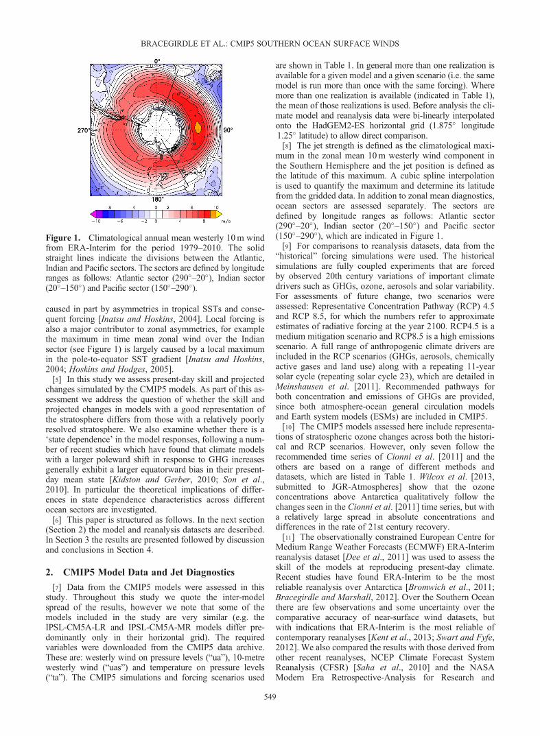
[13] The climatological zonal mean annual mean westerly10m wind from historical CMIP5 model runs is shown inFigure 2a. Compared with ERA-Interim, the ensemble meanposition of the surface jet in the CMIP5 models shows anequatorward bias of 3.3� 1.9� in latitude (where the rangeshown is the inter-model standard deviation). Every ensem-ble member shows an equatorward bias, ranging from 0.4�in NorESM1-M to 7.7� in IPSL-CM5A-LR. There is a largespread in climatological jet strength in the models, withvalues ranging from 5.0 to 9.7m s�1. The weak negativeensemble mean strength bias of �0.4� 1.0m s�1 is smallcompared with the inter-model standard deviation. The skillof the models in reproducing observed position and strength

varies: for example, the NorESM1-M model is the mostaccurate in terms of position but shows the second largestpositive strength bias.[14] For ocean-atmosphere interactions it is important to

consider how wind biases are distributed across the differentocean basins; this is also useful to help elucidate theprocesses leading to the biases. From Figure 2b–d it is clearthat the characteristics of position and strength vary across dif-ferent sectors of the Southern Ocean. The most notable featureis the contrast between large equatorward biases in surface jetposition over the Indian (3.4� 1.6�) and Pacific (3.3� 2.7�)sectors (Figures 2c and 2d, respectively) and a small bias overthe Atlantic sector (1.4� 1.5�). Despite the large position biasover the Indian sector, the ensemble mean jet strength agreesclosely with ERA-Interim (bias of 0.1� 1.0m s�1). Agree-ment in jet strength is also good over the Atlantic sector (biasof 0.3� 1.0m s�1), however it is too weak over the Pacificsector (bias of �1.4� 1.2m s�1). Other recently producedreanalysis datasets (MERRA and CFSR) show results in verygood agreement with those based on ERA-Interim (Figure 2).Even taking into account the fact that the observational uncer-tainties are probably larger than the inter-reanalysis differencesshown here [Kent et al., 2013], it is clear that the inter-CMIP5differences dominate the comparisons.

3.2. Relative Skill of Coupled and Atmosphere-OnlySimulations

[15] The surface jet is associated with the mid-latitudestorm track, which is driven by baroclinic eddies. Many fac-tors, both local and remote, can exert an influence on the

Figure 2. (a) Zonalmean annualmean 10mwesterlywind climatology for the period 1985–2004 as a functionof latitude. (b), (c) and (d) show the same but for the Atlantic, Indian and Pacific sectors, respectively (note thedifferent scales on the y axes). The colored solid and dashed lines indicate the CMIP5 models with overlaid starsymbols indicating high-top models. The black solid, dotted and dashed lines show output from ERA-Interim,CFSR and MERRA, respectively. The arrows indicate double maxima exhibited by model 28 (MRI-CGCM3).


550

climatological location and strength of the baroclinic eddies andthe associated jet. Thus determiningwhat aspects of the coupledmodels might lead to the biases in the surface jet is not straight-forward, particularly in a coupled modelling framework.[16] To investigate the importance of lower boundary

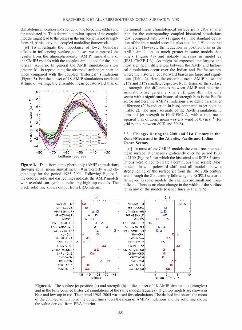
effects in influencing surface jet biases we compared theresults from the atmosphere-only (AMIP) simulations ofthe CMIP5 models with the coupled simulations for the “his-torical” scenario. In general the AMIP simulations showgreater skill in reproducing the observed surface jet positionwhen compared with the coupled “historical” simulations(Figure 3). For the subset of 18 AMIP simulations availableat time of writing, the ensemble mean equatorward bias of

the annual mean climatological surface jet is 28% smallerthan for the corresponding coupled historical simulations(2.4� compared with 3.4�) (Figure 4a). The standard devia-tion of the inter-model spread is also smaller, 1.9� comparedwith 2.2�. However, the reduction in position bias in theAMIP simulations is much greater in some models thanothers (Figure 4a) and notably increases in model 22(IPSL-CM5B-LR). As might be expected, the largest andmost significant differences between the AMIP and histori-cal simulations occur over the Indian and Pacific sectors,where the historical equatorward biases are large and signif-icant (Table 2). Here, the ensemble mean AMIP biases are21% and 31% smaller, respectively. In terms of the surfacejet strength, the differences between AMIP and historicalsimulations are generally smaller (Figure 4b). The onlysector with a significant historical strength bias is the Pacificsector and here the AMIP simulations also exhibit a smallerdifference (20% reduction in bias) compared to jet position(Table 2). The most accurate of the AMIP simulations interms of jet strength is HadGEM2-A, with a root meansquared bias of zonal mean westerly wind of 0.7m s�1 (forgrid-points between 80�S and 30�S).

3.3. Changes During the 20th and 21st Century in theZonal-Mean and in the Atlantic, Pacific and IndianOcean Sectors

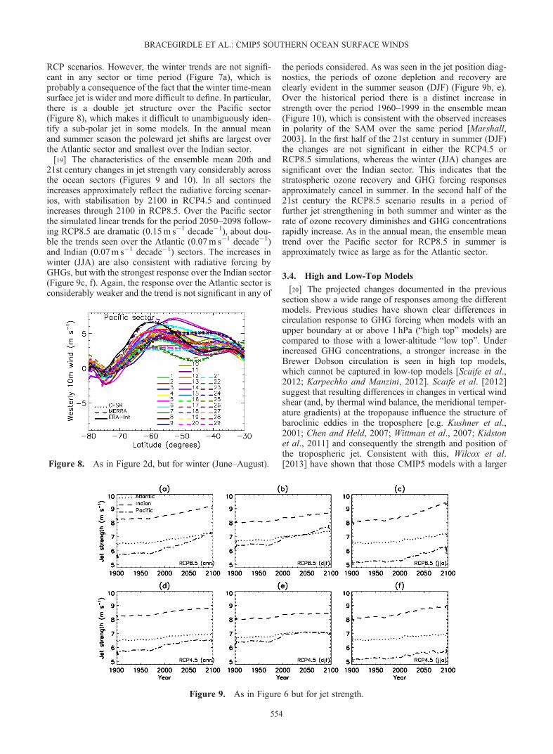
[17] In most of the CMIP5 models the zonal mean annualmean surface jet changes significantly over the period 1900to 2100 (Figure 5, for which the historical and RCP8.5 simu-lations were joined to create a continuous time series). Mostmodels show a poleward shift and all models show astrengthening of the surface jet from the late 20th centuryand through the 21st century following the RCP8.5 scenario.However, in some models, the changes are small and insig-nificant. There is no clear change in the width of the surfacejet in any of the models (dashed lines in Figure 5).

Figure 3. Data from atmosphere-only (AMIP) simulationsshowing zonal mean annual mean 10m westerly wind cli-matology for the period 1985–2004. Following Figure 2,the colored solid and dashed lines indicate the AMIP modelswith overlaid star symbols indicating high top models. Theblack solid line shows output from ERA-Interim.

Figure 4. The surface jet position (a) and strength (b) in the subset of 18 AMIP simulations (triangles)and in the fully coupled historical simulations of the same models (squares). High top models are shown inblue and low top in red. The period 1985–2004 was used for calculations. The dashed line shows the meanof the coupled simulations, the dotted line shows the mean of AMIP simulations and the solid line showsthe value derived from ERA-Interim.


551

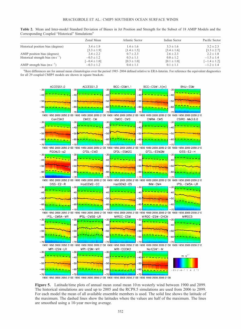
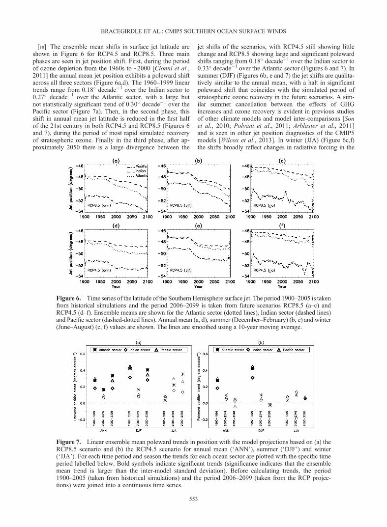
Table 2. Mean and Inter-model Standard Deviation of Biases in Jet Position and Strength for the Subset of 18 AMIP Models and theCorresponding Coupled “Historical” Simulationsa

Zonal Mean Atlantic Sector Indian Sector Pacific Sector

Historical position bias (degrees) 3.4� 1.9 1.4� 1.6 3.3� 1.6 3.2� 2.3[3.3� 1.9] [1.4� 1.5] [3.4� 1.6] [3.3� 2.7]

AMIP position bias (degrees) 2.4� 2.2 0.7� 2.3 2.6� 2.3 2.2� 1.8Historical strength bias (m s�1) �0.5� 1.2 0.3� 1.1 0.0� 1.2 �1.5� 1.4

[�0.4� 1.0] [0.3� 1.0] [0.1� 1.0] [�1.4� 1.2]AMIP strength bias (m s�1) �0.3� 1.2 0.4� 1.1 0.1� 1.1 �1.2� 1.4

aHere differences are for annual mean climatologies over the period 1985–2004 defined relative to ERA-Interim. For reference the equivalent diagnosticsfor all 29 coupled CMIP5 models are shown in square brackets.

Figure 5. Latitude/time plots of annual mean zonal mean 10m westerly wind between 1900 and 2099.The historical simulations are used up to 2005 and the RCP8.5 simulations are used from 2006 to 2099.For each model the mean of all available ensemble members is used. The solid line shows the latitude ofthe maximum. The dashed lines show the latitudes where the values are half of the maximum. The linesare smoothed using a 10-year moving average.


552

[18] The ensemble mean shifts in surface jet latitude areshown in Figure 6 for RCP4.5 and RCP8.5. Three mainphases are seen in jet position shift. First, during the periodof ozone depletion from the 1960s to ~2000 [Cionni et al.,2011] the annual mean jet position exhibits a poleward shiftacross all three sectors (Figure 6a,d). The 1960–1999 lineartrends range from 0.18� decade�1 over the Indian sector to0.27� decade�1 over the Atlantic sector, with a large butnot statistically significant trend of 0.30� decade�1 over thePacific sector (Figure 7a). Then, in the second phase, thisshift in annual mean jet latitude is reduced in the first halfof the 21st century in both RCP4.5 and RCP8.5 (Figures 6and 7), during the period of most rapid simulated recoveryof stratospheric ozone. Finally in the third phase, after ap-proximately 2050 there is a large divergence between the

jet shifts of the scenarios, with RCP4.5 still showing littlechange and RCP8.5 showing large and significant polewardshifts ranging from 0.18� decade�1 over the Indian sector to0.33� decade�1 over the Atlantic sector (Figures 6 and 7). Insummer (DJF) (Figures 6b, e and 7) the jet shifts are qualita-tively similar to the annual mean, with a halt in significantpoleward shift that coincides with the simulated period ofstratospheric ozone recovery in the future scenarios. A sim-ilar summer cancellation between the effects of GHGincreases and ozone recovery is evident in previous studiesof other climate models and model inter-comparisons [Sonet al., 2010; Polvani et al., 2011; Arblaster et al., 2011]and is seen in other jet position diagnostics of the CMIP5models [Wilcox et al., 2013]. In winter (JJA) (Figure 6c,f)the shifts broadly reflect changes in radiative forcing in the

Figure 6. Time series of the latitude of the Southern Hemisphere surface jet. The period 1900–2005 is takenfrom historical simulations and the period 2006–2099 is taken from future scenarios RCP8.5 (a–c) andRCP4.5 (d–f). Ensemble means are shown for the Atlantic sector (dotted lines), Indian sector (dashed lines)and Pacific sector (dashed-dotted lines). Annual mean (a, d), summer (December–February) (b, e) and winter(June–August) (c, f) values are shown. The lines are smoothed using a 10-year moving average.

Figure 7. Linear ensemble mean poleward trends in position with the model projections based on (a) theRCP8.5 scenario and (b) the RCP4.5 scenario for annual mean (‘ANN’), summer (‘DJF’) and winter(‘JJA’). For each time period and season the trends for each ocean sector are plotted with the specific timeperiod labelled below. Bold symbols indicate significant trends (significance indicates that the ensemblemean trend is larger than the inter-model standard deviation). Before calculating trends, the period1900–2005 (taken from historical simulations) and the period 2006–2099 (taken from the RCP projec-tions) were joined into a continuous time series.


553

RCP scenarios. However, the winter trends are not signifi-cant in any sector or time period (Figure 7a), which isprobably a consequence of the fact that the winter time-meansurface jet is wider and more difficult to define. In particular,there is a double jet structure over the Pacific sector(Figure 8), which makes it difficult to unambiguously iden-tify a sub-polar jet in some models. In the annual meanand summer season the poleward jet shifts are largest overthe Atlantic sector and smallest over the Indian sector.[19] The characteristics of the ensemble mean 20th and

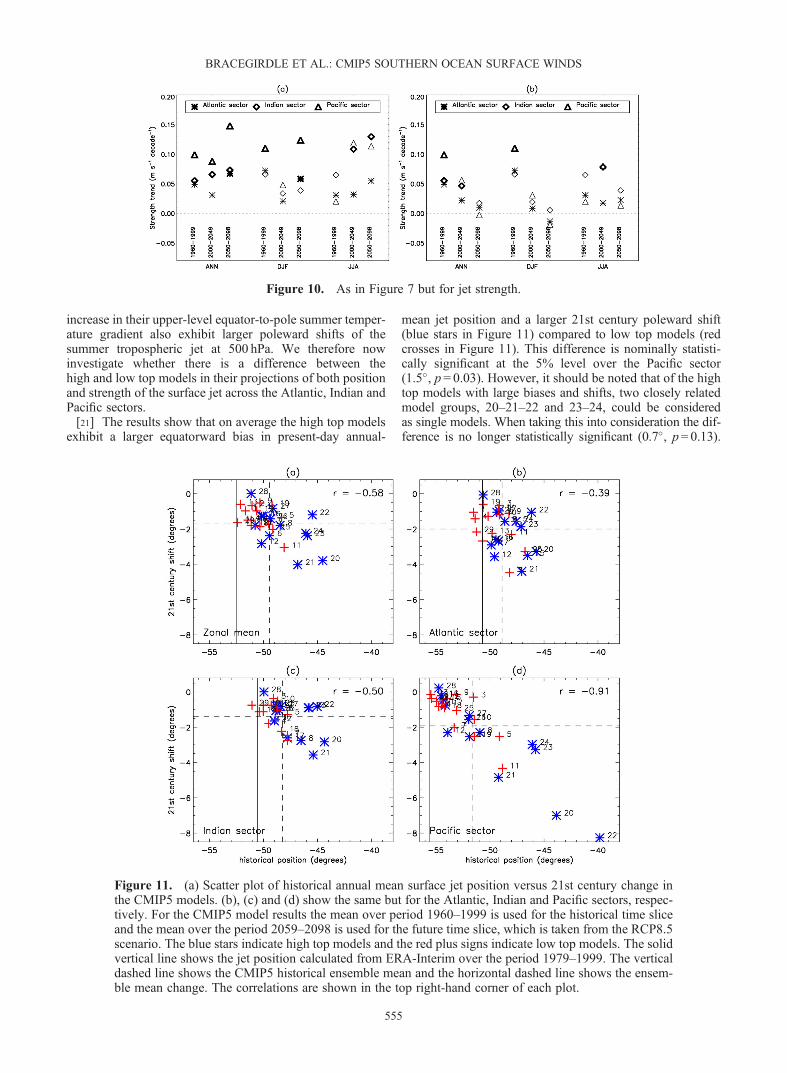
21st century changes in jet strength vary considerably acrossthe ocean sectors (Figures 9 and 10). In all sectors theincreases approximately reflect the radiative forcing scenar-ios, with stabilisation by 2100 in RCP4.5 and continuedincreases through 2100 in RCP8.5. Over the Pacific sectorthe simulated linear trends for the period 2050–2098 follow-ing RCP8.5 are dramatic (0.15m s�1 decade�1), about dou-ble the trends seen over the Atlantic (0.07m s�1 decade�1)and Indian (0.07m s�1 decade�1) sectors. The increases inwinter (JJA) are also consistent with radiative forcing byGHGs, but with the strongest response over the Indian sector(Figure 9c, f). Again, the response over the Atlantic sector isconsiderably weaker and the trend is not significant in any of

the periods considered. As was seen in the jet position diag-nostics, the periods of ozone depletion and recovery areclearly evident in the summer season (DJF) (Figure 9b, e).Over the historical period there is a distinct increase instrength over the period 1960–1999 in the ensemble mean(Figure 10), which is consistent with the observed increasesin polarity of the SAM over the same period [Marshall,2003]. In the first half of the 21st century in summer (DJF)the changes are not significant in either the RCP4.5 orRCP8.5 simulations, whereas the winter (JJA) changes aresignificant over the Indian sector. This indicates that thestratospheric ozone recovery and GHG forcing responsesapproximately cancel in summer. In the second half of the21st century the RCP8.5 scenario results in a period offurther jet strengthening in both summer and winter as therate of ozone recovery diminishes and GHG concentrationsrapidly increase. As in the annual mean, the ensemble meantrend over the Pacific sector for RCP8.5 in summer isapproximately twice as large as for the Atlantic sector.

3.4. High and Low-Top Models

[20] The projected changes documented in the previoussection show a wide range of responses among the differentmodels. Previous studies have shown clear differences incirculation response to GHG forcing when models with anupper boundary at or above 1 hPa (“high top” models) arecompared to those with a lower-altitude “low top”. Underincreased GHG concentrations, a stronger increase in theBrewer Dobson circulation is seen in high top models,which cannot be captured in low-top models [Scaife et al.,2012; Karpechko and Manzini, 2012]. Scaife et al. [2012]suggest that resulting differences in changes in vertical windshear (and, by thermal wind balance, the meridional temper-ature gradients) at the tropopause influence the structure ofbaroclinic eddies in the troposphere [e.g. Kushner et al.,2001; Chen and Held, 2007; Wittman et al., 2007; Kidstonet al., 2011] and consequently the strength and position ofthe tropospheric jet. Consistent with this, Wilcox et al.[2013] have shown that those CMIP5 models with a largerFigure 8. As in Figure 2d, but for winter (June–August).

Figure 9. As in Figure 6 but for jet strength.


554

increase in their upper-level equator-to-pole summer temper-ature gradient also exhibit larger poleward shifts of thesummer tropospheric jet at 500 hPa. We therefore nowinvestigate whether there is a difference between thehigh and low top models in their projections of both positionand strength of the surface jet across the Atlantic, Indian andPacific sectors.[21] The results show that on average the high top models

exhibit a larger equatorward bias in present-day annual-

mean jet position and a larger 21st century poleward shift(blue stars in Figure 11) compared to low top models (redcrosses in Figure 11). This difference is nominally statisti-cally significant at the 5% level over the Pacific sector(1.5�, p= 0.03). However, it should be noted that of the hightop models with large biases and shifts, two closely relatedmodel groups, 20–21–22 and 23–24, could be consideredas single models. When taking this into consideration the dif-ference is no longer statistically significant (0.7�, p=0.13).

Figure 10. As in Figure 7 but for jet strength.

Figure 11. (a) Scatter plot of historical annual mean surface jet position versus 21st century change inthe CMIP5 models. (b), (c) and (d) show the same but for the Atlantic, Indian and Pacific sectors, respec-tively. For the CMIP5 model results the mean over period 1960–1999 is used for the historical time sliceand the mean over the period 2059–2098 is used for the future time slice, which is taken from the RCP8.5scenario. The blue stars indicate high top models and the red plus signs indicate low top models. The solidvertical line shows the jet position calculated from ERA-Interim over the period 1979–1999. The verticaldashed line shows the CMIP5 historical ensemble mean and the horizontal dashed line shows the ensem-ble mean change. The correlations are shown in the top right-hand corner of each plot.


555

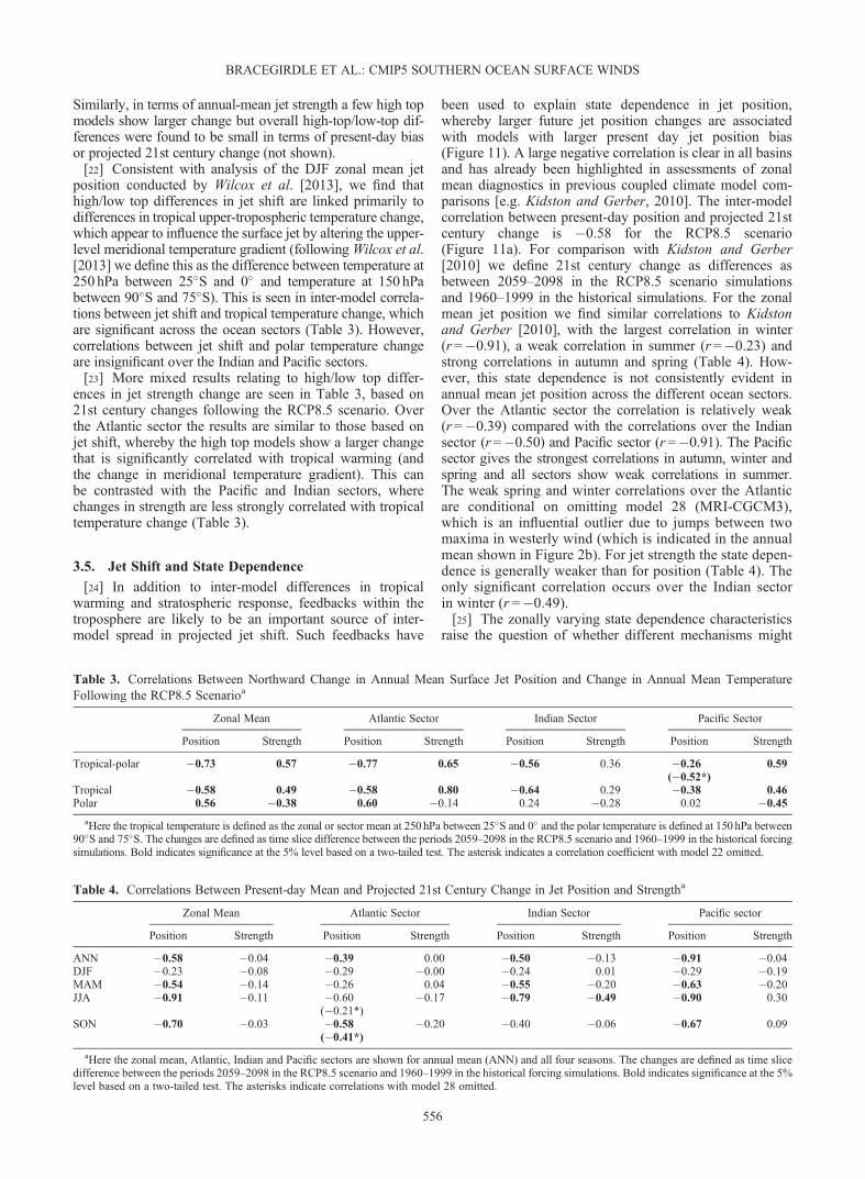
Similarly, in terms of annual-mean jet strength a few high topmodels show larger change but overall high-top/low-top dif-ferences were found to be small in terms of present-day biasor projected 21st century change (not shown).[22] Consistent with analysis of the DJF zonal mean jet

position conducted by Wilcox et al. [2013], we find thathigh/low top differences in jet shift are linked primarily todifferences in tropical upper-tropospheric temperature change,which appear to influence the surface jet by altering the upper-level meridional temperature gradient (followingWilcox et al.[2013] we define this as the difference between temperature at250 hPa between 25�S and 0� and temperature at 150 hPabetween 90�S and 75�S). This is seen in inter-model correla-tions between jet shift and tropical temperature change, whichare significant across the ocean sectors (Table 3). However,correlations between jet shift and polar temperature changeare insignificant over the Indian and Pacific sectors.[23] More mixed results relating to high/low top differ-

ences in jet strength change are seen in Table 3, based on21st century changes following the RCP8.5 scenario. Overthe Atlantic sector the results are similar to those based onjet shift, whereby the high top models show a larger changethat is significantly correlated with tropical warming (andthe change in meridional temperature gradient). This canbe contrasted with the Pacific and Indian sectors, wherechanges in strength are less strongly correlated with tropicaltemperature change (Table 3).

3.5. Jet Shift and State Dependence

[24] In addition to inter-model differences in tropicalwarming and stratospheric response, feedbacks within thetroposphere are likely to be an important source of inter-model spread in projected jet shift. Such feedbacks have

been used to explain state dependence in jet position,whereby larger future jet position changes are associatedwith models with larger present day jet position bias(Figure 11). A large negative correlation is clear in all basinsand has already been highlighted in assessments of zonalmean diagnostics in previous coupled climate model com-parisons [e.g. Kidston and Gerber, 2010]. The inter-modelcorrelation between present-day position and projected 21stcentury change is �0.58 for the RCP8.5 scenario(Figure 11a). For comparison with Kidston and Gerber[2010] we define 21st century change as differences asbetween 2059–2098 in the RCP8.5 scenario simulationsand 1960–1999 in the historical simulations. For the zonalmean jet position we find similar correlations to Kidstonand Gerber [2010], with the largest correlation in winter(r=�0.91), a weak correlation in summer (r =�0.23) andstrong correlations in autumn and spring (Table 4). How-ever, this state dependence is not consistently evident inannual mean jet position across the different ocean sectors.Over the Atlantic sector the correlation is relatively weak(r=�0.39) compared with the correlations over the Indiansector (r=�0.50) and Pacific sector (r=�0.91). The Pacificsector gives the strongest correlations in autumn, winter andspring and all sectors show weak correlations in summer.The weak spring and winter correlations over the Atlanticare conditional on omitting model 28 (MRI-CGCM3),which is an influential outlier due to jumps between twomaxima in westerly wind (which is indicated in the annualmean shown in Figure 2b). For jet strength the state depen-dence is generally weaker than for position (Table 4). Theonly significant correlation occurs over the Indian sectorin winter (r =�0.49).[25] The zonally varying state dependence characteristics

raise the question of whether different mechanisms might

Table 3. Correlations Between Northward Change in Annual Mean Surface Jet Position and Change in Annual Mean TemperatureFollowing the RCP8.5 Scenarioa

Zonal Mean Atlantic Sector Indian Sector Pacific Sector

Position Strength Position Strength Position Strength Position Strength

Tropical-polar �0.73 0.57 �0.77 0.65 �0.56 0.36 �0.26 0.59(�0.52*)

Tropical �0.58 0.49 �0.58 0.80 �0.64 0.29 �0.38 0.46Polar 0.56 �0.38 0.60 �0.14 0.24 �0.28 0.02 �0.45

aHere the tropical temperature is defined as the zonal or sector mean at 250 hPa between 25�S and 0� and the polar temperature is defined at 150 hPa between90�S and 75�S. The changes are defined as time slice difference between the periods 2059–2098 in the RCP8.5 scenario and 1960–1999 in the historical forcingsimulations. Bold indicates significance at the 5% level based on a two-tailed test. The asterisk indicates a correlation coefficient with model 22 omitted.

Table 4. Correlations Between Present-day Mean and Projected 21st Century Change in Jet Position and Strengtha

Zonal Mean Atlantic Sector Indian Sector Pacific sector

Position Strength Position Strength Position Strength Position Strength

ANN �0.58 �0.04 �0.39 0.00 �0.50 �0.13 �0.91 �0.04DJF �0.23 �0.08 �0.29 �0.00 �0.24 0.01 �0.29 �0.19MAM �0.54 �0.14 �0.26 0.04 �0.55 �0.20 �0.63 �0.20JJA �0.91 �0.11 �0.60 �0.17 �0.79 �0.49 �0.90 0.30

(�0.21*)SON �0.70 �0.03 �0.58 �0.20 �0.40 �0.06 �0.67 0.09

(�0.41*)

aHere the zonal mean, Atlantic, Indian and Pacific sectors are shown for annual mean (ANN) and all four seasons. The changes are defined as time slicedifference between the periods 2059–2098 in the RCP8.5 scenario and 1960–1999 in the historical forcing simulations. Bold indicates significance at the 5%level based on a two-tailed test. The asterisks indicate correlations with model 28 omitted.


556

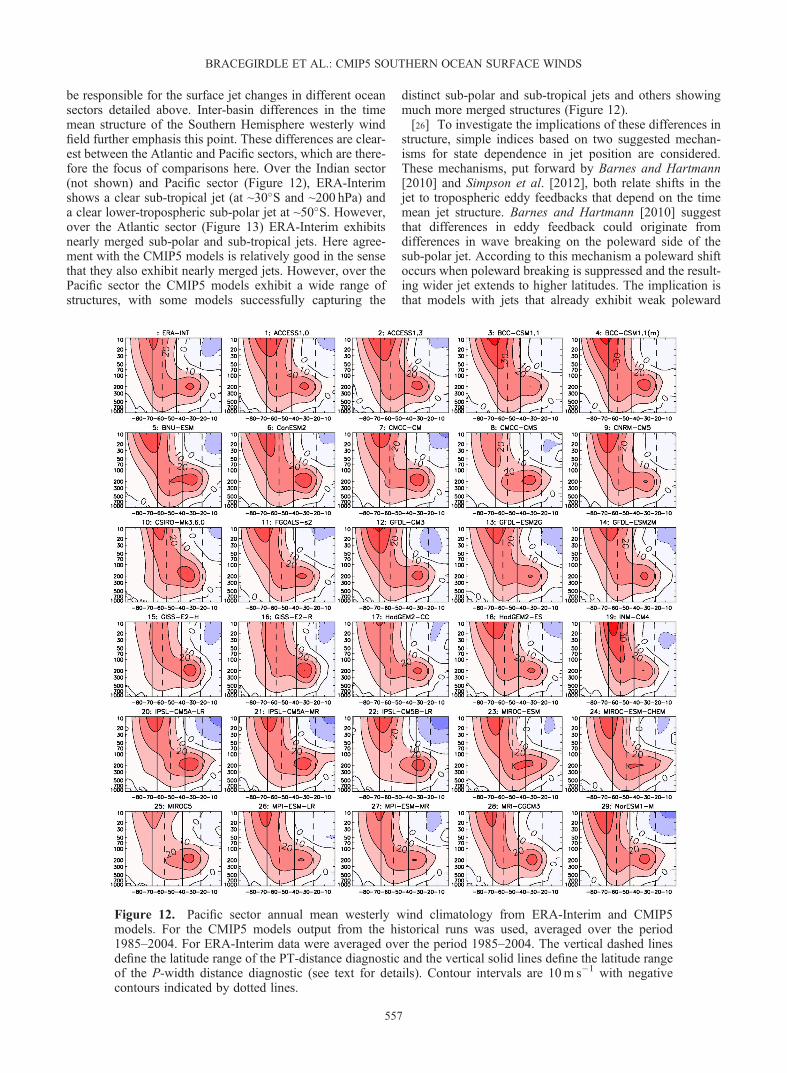
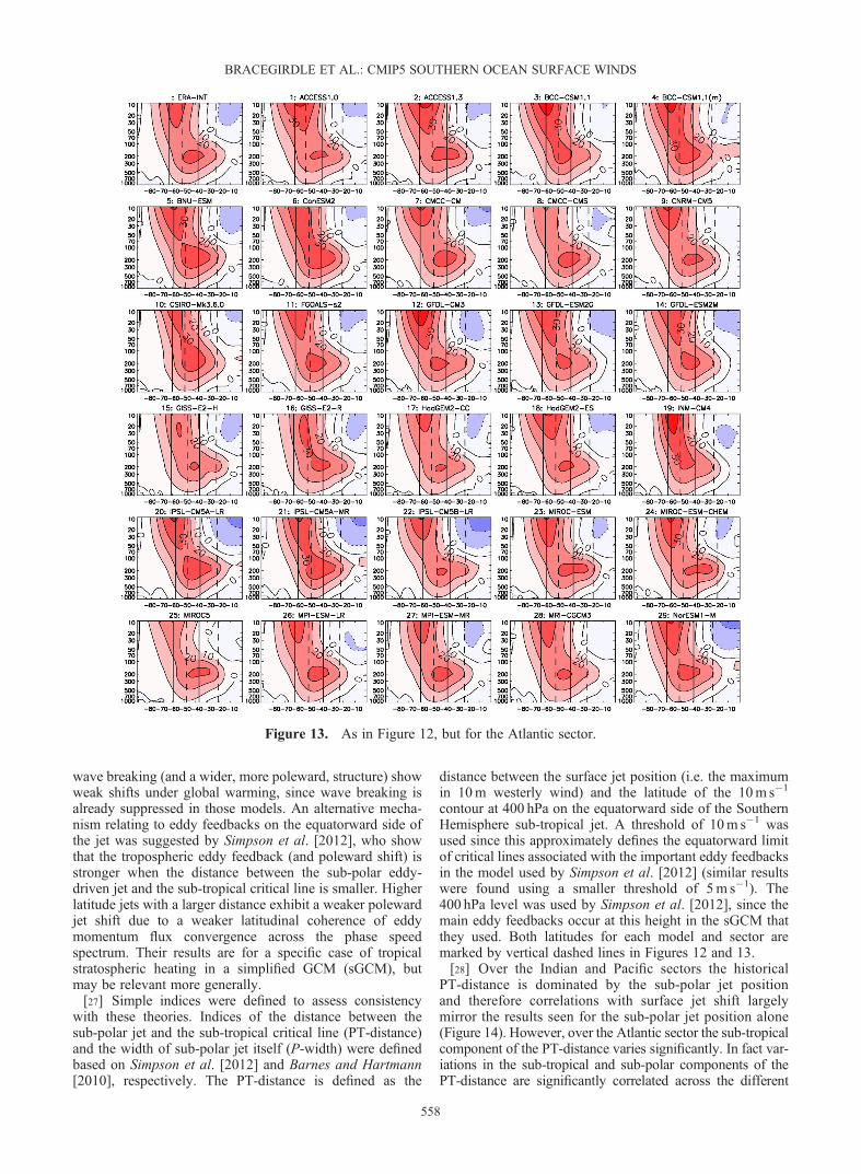
be responsible for the surface jet changes in different oceansectors detailed above. Inter-basin differences in the timemean structure of the Southern Hemisphere westerly windfield further emphasis this point. These differences are clear-est between the Atlantic and Pacific sectors, which are there-fore the focus of comparisons here. Over the Indian sector(not shown) and Pacific sector (Figure 12), ERA-Interimshows a clear sub-tropical jet (at ~30�S and ~200 hPa) anda clear lower-tropospheric sub-polar jet at ~50�S. However,over the Atlantic sector (Figure 13) ERA-Interim exhibitsnearly merged sub-polar and sub-tropical jets. Here agree-ment with the CMIP5 models is relatively good in the sensethat they also exhibit nearly merged jets. However, over thePacific sector the CMIP5 models exhibit a wide range ofstructures, with some models successfully capturing the

distinct sub-polar and sub-tropical jets and others showingmuch more merged structures (Figure 12).[26] To investigate the implications of these differences in

structure, simple indices based on two suggested mechan-isms for state dependence in jet position are considered.These mechanisms, put forward by Barnes and Hartmann[2010] and Simpson et al. [2012], both relate shifts in thejet to tropospheric eddy feedbacks that depend on the timemean jet structure. Barnes and Hartmann [2010] suggestthat differences in eddy feedback could originate fromdifferences in wave breaking on the poleward side of thesub-polar jet. According to this mechanism a poleward shiftoccurs when poleward breaking is suppressed and the result-ing wider jet extends to higher latitudes. The implication isthat models with jets that already exhibit weak poleward

Figure 12. Pacific sector annual mean westerly wind climatology from ERA-Interim and CMIP5models. For the CMIP5 models output from the historical runs was used, averaged over the period1985–2004. For ERA-Interim data were averaged over the period 1985–2004. The vertical dashed linesdefine the latitude range of the PT-distance diagnostic and the vertical solid lines define the latitude rangeof the P-width distance diagnostic (see text for details). Contour intervals are 10m s�1 with negativecontours indicated by dotted lines.


557

wave breaking (and a wider, more poleward, structure) showweak shifts under global warming, since wave breaking isalready suppressed in those models. An alternative mecha-nism relating to eddy feedbacks on the equatorward side ofthe jet was suggested by Simpson et al. [2012], who showthat the tropospheric eddy feedback (and poleward shift) isstronger when the distance between the sub-polar eddy-driven jet and the sub-tropical critical line is smaller. Higherlatitude jets with a larger distance exhibit a weaker polewardjet shift due to a weaker latitudinal coherence of eddymomentum flux convergence across the phase speedspectrum. Their results are for a specific case of tropicalstratospheric heating in a simplified GCM (sGCM), butmay be relevant more generally.[27] Simple indices were defined to assess consistency

with these theories. Indices of the distance between thesub-polar jet and the sub-tropical critical line (PT-distance)and the width of sub-polar jet itself (P-width) were definedbased on Simpson et al. [2012] and Barnes and Hartmann[2010], respectively. The PT-distance is defined as the

distance between the surface jet position (i.e. the maximumin 10m westerly wind) and the latitude of the 10m s�1

contour at 400 hPa on the equatorward side of the SouthernHemisphere sub-tropical jet. A threshold of 10m s�1 wasused since this approximately defines the equatorward limitof critical lines associated with the important eddy feedbacksin the model used by Simpson et al. [2012] (similar resultswere found using a smaller threshold of 5m s�1). The400 hPa level was used by Simpson et al. [2012], since themain eddy feedbacks occur at this height in the sGCM thatthey used. Both latitudes for each model and sector aremarked by vertical dashed lines in Figures 12 and 13.[28] Over the Indian and Pacific sectors the historical

PT-distance is dominated by the sub-polar jet positionand therefore correlations with surface jet shift largelymirror the results seen for the sub-polar jet position alone(Figure 14). However, over the Atlantic sector the sub-tropicalcomponent of the PT-distance varies significantly. In fact var-iations in the sub-tropical and sub-polar components of thePT-distance are significantly correlated across the different

Figure 13. As in Figure 12, but for the Atlantic sector.


558

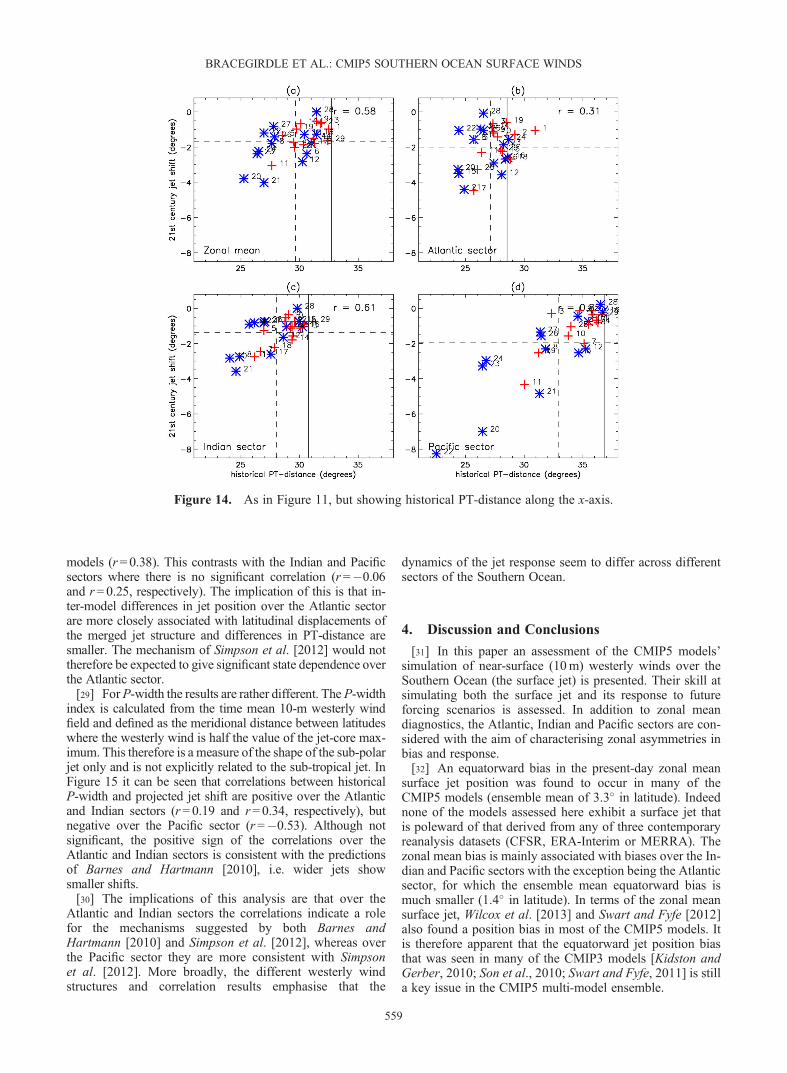
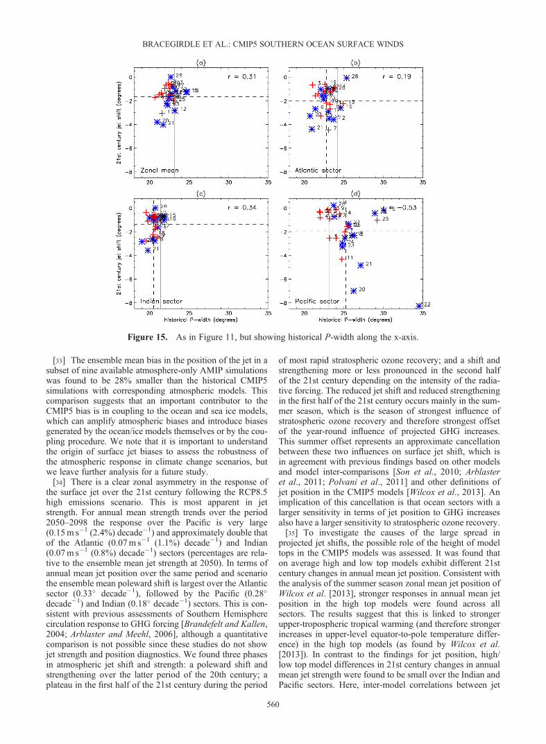
models (r=0.38). This contrasts with the Indian and Pacificsectors where there is no significant correlation (r=�0.06and r=0.25, respectively). The implication of this is that in-ter-model differences in jet position over the Atlantic sectorare more closely associated with latitudinal displacements ofthe merged jet structure and differences in PT-distance aresmaller. The mechanism of Simpson et al. [2012] would nottherefore be expected to give significant state dependence overthe Atlantic sector.[29] For P-width the results are rather different. The P-width

index is calculated from the time mean 10-m westerly windfield and defined as the meridional distance between latitudeswhere the westerly wind is half the value of the jet-core max-imum. This therefore is a measure of the shape of the sub-polarjet only and is not explicitly related to the sub-tropical jet. InFigure 15 it can be seen that correlations between historicalP-width and projected jet shift are positive over the Atlanticand Indian sectors (r=0.19 and r=0.34, respectively), butnegative over the Pacific sector (r=�0.53). Although notsignificant, the positive sign of the correlations over theAtlantic and Indian sectors is consistent with the predictionsof Barnes and Hartmann [2010], i.e. wider jets showsmaller shifts.[30] The implications of this analysis are that over the

Atlantic and Indian sectors the correlations indicate a rolefor the mechanisms suggested by both Barnes andHartmann [2010] and Simpson et al. [2012], whereas overthe Pacific sector they are more consistent with Simpsonet al. [2012]. More broadly, the different westerly windstructures and correlation results emphasise that the

dynamics of the jet response seem to differ across differentsectors of the Southern Ocean.

4. Discussion and Conclusions

[31] In this paper an assessment of the CMIP5 models’simulation of near-surface (10m) westerly winds over theSouthern Ocean (the surface jet) is presented. Their skill atsimulating both the surface jet and its response to futureforcing scenarios is assessed. In addition to zonal meandiagnostics, the Atlantic, Indian and Pacific sectors are con-sidered with the aim of characterising zonal asymmetries inbias and response.[32] An equatorward bias in the present-day zonal mean

surface jet position was found to occur in many of theCMIP5 models (ensemble mean of 3.3� in latitude). Indeednone of the models assessed here exhibit a surface jet thatis poleward of that derived from any of three contemporaryreanalysis datasets (CFSR, ERA-Interim or MERRA). Thezonal mean bias is mainly associated with biases over the In-dian and Pacific sectors with the exception being the Atlanticsector, for which the ensemble mean equatorward bias ismuch smaller (1.4� in latitude). In terms of the zonal meansurface jet, Wilcox et al. [2013] and Swart and Fyfe [2012]also found a position bias in most of the CMIP5 models. Itis therefore apparent that the equatorward jet position biasthat was seen in many of the CMIP3 models [Kidston andGerber, 2010; Son et al., 2010; Swart and Fyfe, 2011] is stilla key issue in the CMIP5 multi-model ensemble.

Figure 14. As in Figure 11, but showing historical PT-distance along the x-axis.


559

[33] The ensemble mean bias in the position of the jet in asubset of nine available atmosphere-only AMIP simulationswas found to be 28% smaller than the historical CMIP5simulations with corresponding atmospheric models. Thiscomparison suggests that an important contributor to theCMIP5 bias is in coupling to the ocean and sea ice models,which can amplify atmospheric biases and introduce biasesgenerated by the ocean/ice models themselves or by the cou-pling procedure. We note that it is important to understandthe origin of surface jet biases to assess the robustness ofthe atmospheric response in climate change scenarios, butwe leave further analysis for a future study.[34] There is a clear zonal asymmetry in the response of

the surface jet over the 21st century following the RCP8.5high emissions scenario. This is most apparent in jetstrength. For annual mean strength trends over the period2050–2098 the response over the Pacific is very large(0.15m s�1 (2.4%) decade�1) and approximately double thatof the Atlantic (0.07m s�1 (1.1%) decade�1) and Indian(0.07m s�1 (0.8%) decade�1) sectors (percentages are rela-tive to the ensemble mean jet strength at 2050). In terms ofannual mean jet position over the same period and scenariothe ensemble mean poleward shift is largest over the Atlanticsector (0.33� decade�1), followed by the Pacific (0.28�decade�1) and Indian (0.18� decade�1) sectors. This is con-sistent with previous assessments of Southern Hemispherecirculation response to GHG forcing [Brandefelt and Kallen,2004; Arblaster and Meehl, 2006], although a quantitativecomparison is not possible since these studies do not showjet strength and position diagnostics. We found three phasesin atmospheric jet shift and strength: a poleward shift andstrengthening over the latter period of the 20th century; aplateau in the first half of the 21st century during the period

of most rapid stratospheric ozone recovery; and a shift andstrengthening more or less pronounced in the second halfof the 21st century depending on the intensity of the radia-tive forcing. The reduced jet shift and reduced strengtheningin the first half of the 21st century occurs mainly in the sum-mer season, which is the season of strongest influence ofstratospheric ozone recovery and therefore strongest offsetof the year-round influence of projected GHG increases.This summer offset represents an approximate cancellationbetween these two influences on surface jet shift, which isin agreement with previous findings based on other modelsand model inter-comparisons [Son et al., 2010; Arblasteret al., 2011; Polvani et al., 2011] and other definitions ofjet position in the CMIP5 models [Wilcox et al., 2013]. Animplication of this cancellation is that ocean sectors with alarger sensitivity in terms of jet position to GHG increasesalso have a larger sensitivity to stratospheric ozone recovery.[35] To investigate the causes of the large spread in

projected jet shifts, the possible role of the height of modeltops in the CMIP5 models was assessed. It was found thaton average high and low top models exhibit different 21stcentury changes in annual mean jet position. Consistent withthe analysis of the summer season zonal mean jet position ofWilcox et al. [2013], stronger responses in annual mean jetposition in the high top models were found across allsectors. The results suggest that this is linked to strongerupper-tropospheric tropical warming (and therefore strongerincreases in upper-level equator-to-pole temperature differ-ence) in the high top models (as found by Wilcox et al.[2013]). In contrast to the findings for jet position, high/low top model differences in 21st century changes in annualmean jet strength were found to be small over the Indian andPacific sectors. Here, inter-model correlations between jet

Figure 15. As in Figure 11, but showing historical P-width along the x-axis.


560

strength change and tropical temperature change are weakand the polar component of changes in upper-level meridio-nal temperature gradient is more important. This furtheremphasises the role of tropical upper-tropospheric warmingin high/low top differences. However, since the CMIP5models differ in many ways other than model top, it is notpossible to directly attribute the differences between the highand low top subsets to the height of the model lid. In partic-ular, Santer et al. [2012] recently identified inter-modeldifferences in the treatment of ozone (e.g. see Table 1) as akey influence on lower-stratospheric temperature trends inthe CMIP5 models.[36] In addition to inter-model differences in tropical

upper-tropospheric warming and stratospheric response, thetheoretical implications of differences in historical mean-state tropospheric jet structure for projected jet shift wereinvestigated. An inter-model relationship between present-day mean-state bias and projected 21st century change (statedependence) was found in annual mean zonal mean jetposition with a correlation of r =�0.58. This is slightlysmaller than the value obtained by Wilcox et al. [2013](r=�0.64) based on their assessment of 500 hPa jet positionin the CMIP5 models and smaller than the surface jet corre-lations found in the CMIP3 models by Kidston and Gerber[2010] (r =�0.77). The annual cycle of correlations is simi-lar to that found by with Kidston and Gerber [2010], whoused the same diagnostic based on near-surface wind. Whenthe above analysis was extended to individual ocean sectors,it was found that correlations are even stronger over thePacific sector (r=�0.91), but weaker over the Atlanticsector (r =�0.39).[37] The variations in state dependence reflect significant

differences in mean state structure across the differentsectors and help provide some insight into mechanisms forprojected shifts of the jet. The differences in structurewere captured with simple indices of the sub-polar jet width(P-width) and the distance between the sub-polar and sub-tropical jet (PT-distance), which are related to mechanismsfor state dependence suggested by Barnes and Hartmann[2010] and Simpson et al. [2012], respectively. The clearestdifferences are between the Atlantic and Pacific sectors.Over the Atlantic sector the reanalysis and models show aconsistent merged jet structure, with no clear separationbetween the sub-polar and sub-tropical jets (i.e. smallPT-distance). Here projected jet shifts are not significantly cor-related with either P-width (r=0.19) or PT-distance (r=0.31).In contrast over the Pacific sector the CMIP5 models exhibit awide range of structures, with some models successfully cap-turing the distinct sub-polar and sub-tropical jets seen in there-analyses and others showing much more merged structures.Inter-model correlations with projected shifts are much largerfor PT-distance (r=0.85) than P-width (r=�0.28 with outliermodel 22 excluded). The implication of these results is thatdifferent dynamical regimes in the different ocean sectors leadto contrasting mechanisms for projected jet shift. The extent towhich the above mechanisms emerge in full GCMs is notproven here and consistency with these and other theoriesacross the different sectors would require further diagnosticsrelating to baroclinic eddy life cycles and length scales[Wittman et al., 2007; Kidston et al., 2011], internal jetvariability [Kidston and Gerber, 2010; Barnes and Hartmann,2012] and phase speed [Chen and Held, 2007; Simpson et al.,

2012]. It is anticipated that a more comprehensive understand-ing of jet bias and shift across the Southern Ocean may bepossible by not only considering the zonal mean, but focussingon sectors across individual ocean basins.

[38] Acknowledgments. This study is part of the British Antarctic Sur-vey Polar Science for Planet Earth Programme. It was funded by The UKNatural Environment Research Council (grant reference number NE/J005339/1). Three anonymous reviewers are thanked for their commentsand suggestions, which helped to significantly improve the manuscript. Weacknowledge the World Climate Research Programme’s Working Groupon Coupled Modelling, which is responsible for CMIP, and we thank the cli-mate modeling groups for producing and making available their model out-put (listed in Table 1 of this paper). For CMIP the U.S. Department ofEnergy’s Program for Climate Model Diagnosis and Intercomparison pro-vides coordinating support and led development of software infrastructurein partnership with the Global Organization for Earth System Science Por-tals. The European Centre for Medium Range Weather Forecasting arethanked for providing the ERA-40 and ERA-Interim datasets. The GlobalModeling and Assimilation Office (GMAO) and the GESDISC are acknowl-edged for the dissemination of the MERRA dataset. The CFSR data wasretrieved from the Research Data Archive, which is managed by the DataSupport Section of the Computational and Information Systems Laboratoryat the National Center for Atmospheric Research in Boulder, Colorado.

ReferencesArblaster, J. M., and G. A. Meehl (2006), Contributions of external forcingsto southern annular mode trends, J. Clim., 19(12), 2896–2905,doi:10.1175/JCLI3774.1.

Arblaster, J. M., G. A. Meehl, and D. J. Karoly (2011), Future climatechange in the Southern Hemisphere: Competing effects of ozone andgreenhouse gases, Geophys. Res. Lett., 38, L02701, doi:10.1029/2010gl045384.

Barnes, E. A., and D. L. Hartmann (2010), Testing a theory for the effect oflatitude on the persistence of eddy-driven jets using CMIP3 simulations,Geophys. Res. Lett., 37, L15801, doi:10.1029/2010gl044144.

Barnes, E. A., and D. L. Hartmann (2012), Detection of Rossby wave break-ing and its response to shifts of the midlatitude jet with climate change, J.Geophys. Res., 117(D9), D09117, doi:10.1029/2012jd017469.

Bracegirdle, T. J., and G. J. Marshall (2012), The reliability of Antarctic tro-pospheric pressure and temperature in the latest global reanalyses, J.Clim., 25, 7138–7146, doi:10.1175/JCLI-D-11-00685.1.

Bracegirdle, T. J., W. M. Connolley, and J. Turner (2008), Antarctic climatechange over the twenty first century, J. Geophys. Res. Atmos., 113(D3),doi:10.1029/2007jd008933.

Brandefelt, J., and E. Kallen (2004), The response of the Southern Hemi-sphere atmospheric circulation to an enhanced greenhouse gas forcing,J. Clim., 17(22), 4425–4442, doi:10.1175/3221.1.

Bromwich, D. H., J. P. Nicolas, and A. J. Monaghan (2011), An Assessmentof Precipitation Changes over Antarctica and the Southern Ocean since1989 in Contemporary Global Reanalyses, J. Clim., 24(16), 4189–4209,doi:10.1175/2011jcli4074.1.

Chen, G., and I. M. Held (2007), Phase speed spectra and the recent pole-ward shift of Southern Hemisphere surface westerlies, Geophys. Res.Lett., 34(21), L21805, doi:10.1029/2007gl031200.

Ciasto, L. M., and D. W. J. Thompson (2008), Observations of large-scaleocean-atmosphere interaction in the southern hemisphere, J. Clim., 21(6), 1244–1259, doi:10.1175/2007jcl11809.1.

Cionni, I., V. Eyring, J. F. Lamarque, W. J. Randel, D. S. Stevenson, F.Wu, G. E. Bodeker, T. G. Shepherd, D. T. Shindell, and D. W. Waugh(2011), Ozone database in support of CMIP5 simulations: resultsand corresponding radiative forcing, Atmos. Chem. Phys., 11(21),11267–11292, doi:10.5194/acp-11-11267-2011.

Dee, D. P., et al. (2011), The ERA-Interim reanalysis: configuration andperformance of the data assimilation system, Q. J. R. Meteorolog. Soc.,137(656), 553–597, doi:10.1002/qj.828.

Fyfe, J. C., and O. A. Saenko (2006), Simulated changes in the extratropicalSouthern Hemisphere winds and currents, Geophys. Res. Lett., 33,L06701, doi:10.1029/2005GL025332.

Guemas, V., and F. Codron (2011), Differing Impacts of ResolutionChanges in Latitude and Longitude on the Midlatitudes in the LMDZAtmospheric GCM, J. Clim., 24(22), 5831–5849, doi:10.1175/2011jcli4093.1.

Hall, A., and M. Visbeck (2002), Synchronous variability in the SouthernHemisphere atmosphere, sea ice, and ocean resulting from the AnnularMode, J. Clim., 15, 3043–3057, doi:10.1175/1520-0442(2002)015<3043:SVITSH>2.0.CO;2.


561

Hoskins, B. J., and K. I. Hodges (2005), A New Perspective on SouthernHemisphere Storm Tracks, J. Clim., 18, 4108–4129, doi:10.1175/JCLI3570.1.

Hourdin, F., et al. (2012), Impact of the LMDZ atmospheric grid configura-tion on the climate and sensitivity of the IPSL-CM5A coupled model,Clim. Dyn., doi:10.1007/s00382-012-1411-3.

Hurrell, J. W., J. J. Hack, D. Shea, J. M. Caron, and J. Rosinski (2008), Anew sea surface temperature and sea ice boundary dataset for the Commu-nity Atmosphere Model, J. Clim., 21(19), 5145–5153, doi:10.1175/2008jcli2292.1.

Inatsu, M., and B. J. Hoskins (2004), The zonal asymmetry of the SouthernHemisphere winter storm track, J. Clim., 17(24), 4882–4892,doi:10.1175/jcli-3232.1.

Karpechko, A. Y., and E. Manzini (2012), Stratospheric influence on tropo-spheric climate change in the Northern Hemisphere, J. Geophys. Res.Atmos., 117, D05133, doi:10.1029/2011jd017036.

Karpechko, A. Y., N. P. Gillett, G. J. Marshall, and A. Scaife (2008), Strato-spheric influence on circulation changes in the Southern Hemisphere tro-posphere in coupled climate models,Geophys. Res. Lett., 35(20), L20806,doi:10.1029/2008gl035354.

Kawase, H., T. Nagashima, K. Sudo, and T. Nozawa (2011), Future changesin tropospheric ozone under Representative Concentration Pathways(RCPs), Geophys. Res. Lett., 38, L05801, doi:10.1029/2010gl046402.

Kent, E. C., S. Fangohr, and D. I. Berry (2013), A comparative assessmentof monthly mean wind speed products over the global ocean, Int. J.Climatol., in press, doi:10.1002/joc.3606.

Kidston, J., and E. P. Gerber (2010), Intermodel variability of the polewardshift of the austral jet stream in the CMIP3 integrations linked to biases in20th century climatology, Geophys. Res. Lett., 37, L09708, doi:10.1029/2010gl042873.

Kidston, J., G. K. Vallis, S. M. Dean, and J. A. Renwick (2011), Can the In-crease in the Eddy Length Scale under Global Warming Cause the PolewardShift of the Jet Streams?, J. Clim., 24(14), 3764–3780, doi:10.1175/2010jcli3738.1.

Kushner, P. J., I. M. Held, and T. L. Delworth (2001), Southern Hemisphereatmospheric circulation response to global warming, J. Clim., 14, 2238–2249,doi:10.1175/1520-0442(2001)014<0001:SHACRT>2.0.CO;2.

Lamarque, J.-F., G. P. Kyle, M. Meinshausen, K. Riahi, S. J. Smith, D. P.van Vuuren, A. J. Conley, and F. Vitt (2011), Global and regional evolu-tion of short-lived radiatively active gases and aerosols in the Representa-tive Concentration Pathways, Clim. Chang., 109(1-2), 191–212,doi:10.1007/s10584-011-0155-0.

Le Quere, C., et al. (2007), Saturation of the Southern Ocean CO2 Sink Dueto Recent Climate Change, Science, 316(5832), 1735–1738, doi:10.1126/science.1136188.

Lovenduski, N. S., and N. Gruber (2005), Impact of the Southern AnnularMode on Southern Ocean circulation and biology, Geophys. Res. Lett.,32(11), L11603, doi:10.1029/2005gl022727.

Lovenduski, N. S., N. Gruber, S. C. Doney, and I. D. Lima (2007), En-hanced CO(2) outgassing in the Southern Ocean from a positive phaseof the Southern Annular Mode, Global Biogeochem. Cycles, 21(2),Gb2026, doi:10.1029/2006gb002900.

Maloney, E. D., and D. B. Chelton (2006), An assessment of the sea surfacetemperature influence on surface wind stress in numerical weather predic-tion and climate models, J. Clim., 19(12), 2743–2762, doi:10.1175/jcli3728.1.

Marshall, G. J. (2003), Trends in the Southern Annular Mode from observa-tions and reanalyses, J. Clim., 16, 4134–4143, doi:10.1175/1520-0442(2003)016<4134:TITSAM>2.0.CO;2.

Meinshausen, M., et al. (2011), The RCP greenhouse gas concentrationsand their extensions from 1765 to 2300, Clim. Chang., 109(1-2), 213–241,doi:10.1007/s10584-011-0156-z.

Meredith, M. P., and A. M. Hogg (2006), Circumpolar response of SouthernOcean eddy activity to a change in the Southern Annular Mode, Geophys.Res. Lett., 33(16), L16608, doi:10.1029/2006gl026499.

Miller, R. L., G. A. Schmidt, and D. T. Shindell (2006), Forced annular var-iations in the 20th century Intergovernmental Panel on Climate ChangeFourth Assessment Report models, J. Geophys. Res., 111, 10.1029/2005JD006323.

Polvani, L. M., M. Previdi, and C. Deser (2011), Large cancellation, due toozone recovery, of future Southern Hemisphere atmospheric circulationtrends, Geophys. Res. Lett., 38, L04707, doi:10.1029/2011gl046712.

Randel, W. J., and F. Wu (2007), A stratospheric ozone profile data set for1979–2005: Variability, trends, and comparisons with column ozone data,J. Geophys. Res. Atmos., 112(D6), D06313, doi:10.1029/2006jd007339.

Rienecker, M. M., et al. (2011), MERRA: NASA’s Modern-Era Retrospec-tive Analysis for Research and Applications, J. Clim., 24(14), 3624–3648,doi:10.1175/jcli-d-11-00015.1.

Roscoe, H. K., and J. D. Haigh (2007), Influences of ozone depletion, the solarcycle and the QBO on the Southern Annular Mode, Q. J. R. Meteorolog.Soc., 133(628), 1855–1864, doi:10.1002/qj.153.

Saha, S., et al. (2010), The NCEP Climate Forecast System Reanalysis,Bull. Am. Meteorol. Soc., 91(8), 1015–1057, doi:10.1175/2010bams3001.1.

Sallee, J. B., K. Speer, and R. Morrow (2008), Response of the Antarctic Cir-cumpolar Current to atmospheric variability, J. Clim., 21(12), 3020–3039,doi:10.1175/2007jcli1702.1.

Sallee, J. B., K. G. Speer, and S. R. Rintoul (2010), Zonally asymmetric re-sponse of the Southern Ocean mixed-layer depth to the Southern AnnularMode, Nat. Geosci., 3(4), 273–279, doi:10.1038/ngeo812.

Santer, B. D., et al. (2012), Identifying human influences on atmospherictemperature, Proc. Natl. Acad. Sci., doi:10.1073/pnas.1210514109.

Scaife, A., et al. (2012), Climate change projections and stratosphere–troposphereinteraction, Clim. Dyn., 38, 2089–2097, doi:10.1007/s00382-011-1080-7.

Sen Gupta, A., and M. H. England (2006), Coupled ocean-atmosphere-iceresponse to variations in the Southern Annular Mode, J. Clim., 19(18),4457–4486, doi:10.1175/jcli3843.1.

Shindell, T., and G. A. Schmidt (2004), Southern Hemisphere climate re-sponse to ozone changes and greenhouse gas increases, Geophys. Res.Lett., 31, L18209, doi:10.1029/2004GL020724.

Simpson, I. R., M. Blackburn, J. D. Haigh, and S. N. Sparrow (2012),A mechanism for the effect of tropospheric jet structure on the annularmode-like response to stratospheric forcing, J. Atmos. Sci., 69, 2152–2170,doi:10.1175/JAS-D-11-0188.1.

Son, S. W., et al. (2010), Impact of stratospheric ozone on Southern Hemi-sphere circulation change: A multimodel assessment, J. Geophys. Res.Atmos., 115, D00M07, doi:10.1029/2010JD014271.

Stammerjohn, S. E., D. G. Martinson, R. C. Smith, X. Yuan, and D. Rind(2008), Trends in Antarctic annual sea ice retreat and advance and theirrelation to El Nino-Southern Oscillation and Southern Annular Mode var-iability, J. Geophys. Res. Oceans, 113(C3), C03S90, doi:10.1029/2007jc004269.

Swart, N. C., and J. C. Fyfe (2011), Ocean carbon uptake and storage influ-enced by wind bias in global climate models, Nat. Clim. Change, 2(1),47–52, doi:10.1038/nclimate1289.

Swart, N. C., and J. C. Fyfe (2012), Observed and simulated changes in theSouthern Hemisphere surface westerly wind-stress, Geophys. Res. Lett.,39(16), L16711, doi:10.1029/2012gl052810.

Taylor, K. E., D. Williamson, and F. Zwiers (2000), The sea surface tempera-ture and sea-ice concentration boundary conditions for AMIP II simulationsRep. 60, 25pp, Lawrence Livermore National Laboratory, California.

Taylor, K. E., R. J. Stouffer, and G. A. Meehl (2012), An Overviewof CMIP5 and the Experiment Design, Bull. Am. Meteorol. Soc., 93,485–498, doi:10.1175/bams-d-11-00094.1.

Thompson, D. W. J., and S. Solomon (2002), Interpretation of recent South-ern Hemisphere climate change, Science, 296, 895–899, doi:10.1126/science.1069270.

Thompson, D. W. J., S. Solomon, P. J. Kushner, M. H. England, K. M.Grise, and D. J. Karoly (2011), Signatures of the Antarctic ozone holein Southern Hemisphere surface climate change, Nat. Geosci., 4(11),741–749, doi:10.1038/ngeo1296.

Verdy, A., J. Marshall, and A. Czaja (2006), Sea surface temperaturevariability along the path of the antarctic circumpolar current, J. Phys.Oceanogr., 36(7), 1317–1331, doi:10.1175/jpo2913.1.

Wang, Y. H., and G. Magnusdottir (2011), Tropospheric Rossby WaveBreaking and the SAM, J. Clim., 24(8), 2134–2146, doi:10.1175/2010jcli4009.1.

Wang, Z., T. Kuhlbrodt, and M. P. Meredith (2011), On the response of theAntarctic Circumpolar Current transport to climate change in coupledclimate models, J. Geophys. Res., 116, C08011, doi:10.1029/2010JC006757.

Wilcox, L. J., A. J. Charlton-Perez, and L. J. Gray (2013), Trends in Australjet position in ensembles of high- and low-top CMIP5 models, J.Geophys. Res., 117, D13115, doi:10.1029/2012JD017597.

Wittman, M. A. H., A. J. Charlton, and L. M. Polvani (2007), The effect oflower stratospheric shear on baroclinic instability, J. Atmos. Sci., 64(2),479–496, doi:10.1175/jas3828.1.

Yang, X.-Y., R. X. Huang, and D. X. Wang (2007), Decadal changes ofwind stress over the Southern Ocean associated with Antarctic ozone de-pletion, J. Clim., 20(14), 3395–3410, doi:10.1175/jcli4195.1.


562

Documents

Assessment of surface winds over the Atlantic, Indian, and Pacific Ocean sectors of the Southern Ocean in CMIP5 models: historical bias, forcing response, and state dependence