Asset Allocation Framework

8/3/2019 Asset Allocation Framework

http://slidepdf.com/reader/full/asset-allocation-framework 1/13

Foundations of Finance: Asset Allocation: Risky vs. Riskless Prof. Alex Shapiro

1

Lecture Notes 6

Asset Allocation: Risky vs. Riskless

I. Readings and Suggested Practice Problems

II. Expected Portfolio Return: General Formula

III. Standard Deviation of Portfolio Return:

One Risky Asset and a Riskless Asset

IV. The Asset Allocation Framework

V. The Capital Allocation Line

VI. Portfolio Management:


VII. Additional Readings

Buzz Words: Reward to Variability Ratio, Separation Theorem, Portfolio’s Risk Adjustment, Portfolio Management



Foundations of Finance: Asset Allocation: Risky vs. Riskles

2

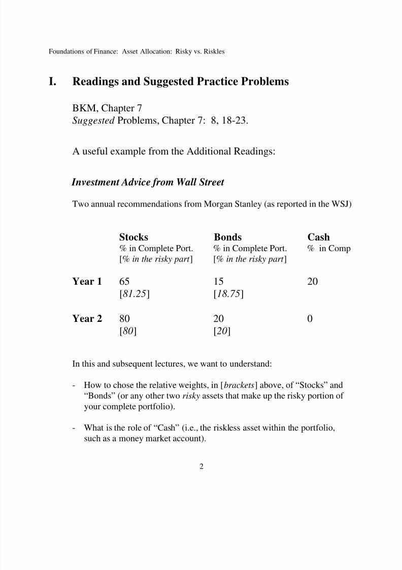
I. Readings and Suggested Practice Problems

BKM, Chapter 7

Suggested Problems, Chapter 7: 8, 18-23.

A useful example from the Additional Readings:

Investment Advice from Wall Street

Two annual recommendations from Morgan Stanley (as reported in the WSJ)

Stocks Bonds Cash% in Complete Port. % in Complete Port. % in Comp

[% in the risky part ] [% in the risky part ]

Year 1 65 15 20

[81.25] [18.75]

Year 2 80 20 0

[80] [20]

In this and subsequent lectures, we want to understand:

- How to chose the relative weights, in [brackets] above, of “Stocks” and

“Bonds” (or any other two risky assets that make up the risky portion of your complete portfolio).

- What is the role of “Cash” (i.e., the riskless asset within the portfolio,such as a money market account).




3

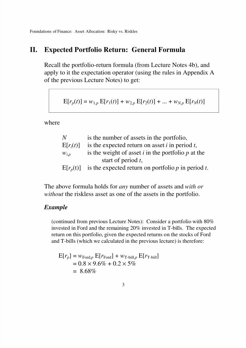
II. Expected Portfolio Return: General Formula

Recall the portfolio-return formula (from Lecture Notes 4b), and

apply to it the expectation operator (using the rules in Appendix A

of the previous Lecture Notes) to get:

E[r p(t )] = w1, p E[r 1(t )] + w2 ,p E[r 2(t )] + ... + w N,p E[r N (t )]

where

N is the number of assets in the portfolio,

E[r i(t )] is the expected return on asset i in period t ,

wi, p is the weight of asset i in the portfolio p at the

start of period t ,

E[r p(t)] is the expected return on portfolio p in period t .

The above formula holds for any number of assets and with or

without the riskless asset as one of the assets in the portfolio.

Example

(continued from previous Lecture Notes): Consider a portfolio with 80%

invested in Ford and the remaining 20% invested in T-bills. The expected

return on this portfolio, given the expected returns on the stocks of Ford

and T-bills (which we calculated in the previous lecture) is therefore:

E[r p] = wFord, p E[r Ford] + wT-bill, p E[r T-bill]

= 0.8 × 9.6% + 0.2 × 5%

= 8.68%




4

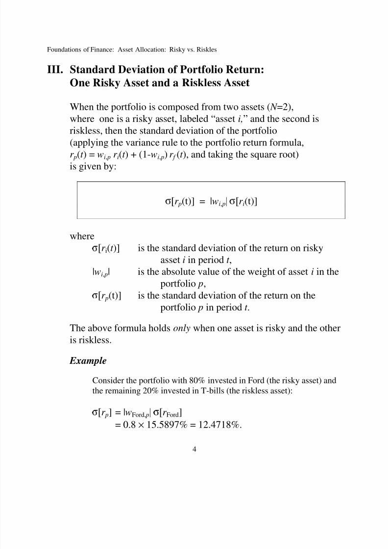
III. Standard Deviation of Portfolio Return:


When the portfolio is composed from two assets ( N =2),

where one is a risky asset, labeled “asset i,” and the second isriskless, then the standard deviation of the portfolio(applying the variance rule to the portfolio return formula,r p(t ) = wi, p r i(t ) + (1-wi, p) r f (t ), and taking the square root)is given by:

>r p(t)] = |wi, p_ >r i(t)]

where>r i(t )] is the standard deviation of the return on risky

asset i in period t ,|wi, p| is the absolute value of the weight of asset i in the

portfolio p,>r p(t)] is the standard deviation of the return on theportfolio p in period t .

The above formula holds only when one asset is risky and the otheris riskless.

Example

Consider the portfolio with 80% invested in Ford (the risky asset) andthe remaining 20% invested in T-bills (the riskless asset):

>r p] = |wFord, p_ >r Ford]

= 0.8 × 15.5897% = 12.4718%.




5

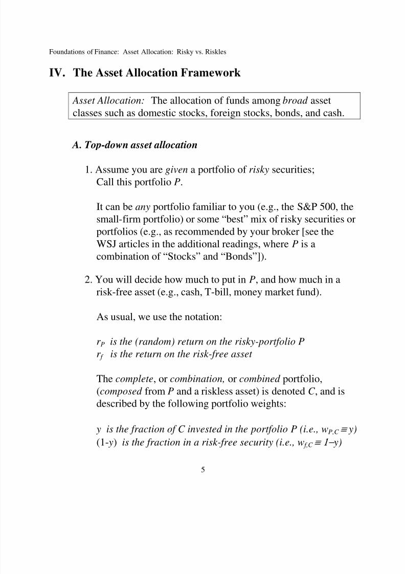
IV. The Asset Allocation Framework

Asset Allocation: The allocation of funds among broad assetclasses such as domestic stocks, foreign stocks, bonds, and cash.

A. Top-down asset allocation

1. Assume you are given a portfolio of risky securities;

Call this portfolio P.

It can be any portfolio familiar to you (e.g., the S&P 500, the

small-firm portfolio) or some “best” mix of risky securities orportfolios (e.g., as recommended by your broker [see theWSJ articles in the additional readings, where P is acombination of “Stocks” and “Bonds”]).

2. You will decide how much to put in P, and how much in arisk-free asset (e.g., cash, T-bill, money market fund).

As usual, we use the notation:

r P is the (random) return on the risky-portfolio P r f is the return on the risk-free asset

The complete, or combination, or combined portfolio,(composed from P and a riskless asset) is denoted C , and is

described by the following portfolio weights:

y is the fraction of C invested in the portfolio P (i.e., wP,C ≡ y)

(1- y) is the fraction in a risk-free security (i.e., w f,C ≡ 1− y)




6

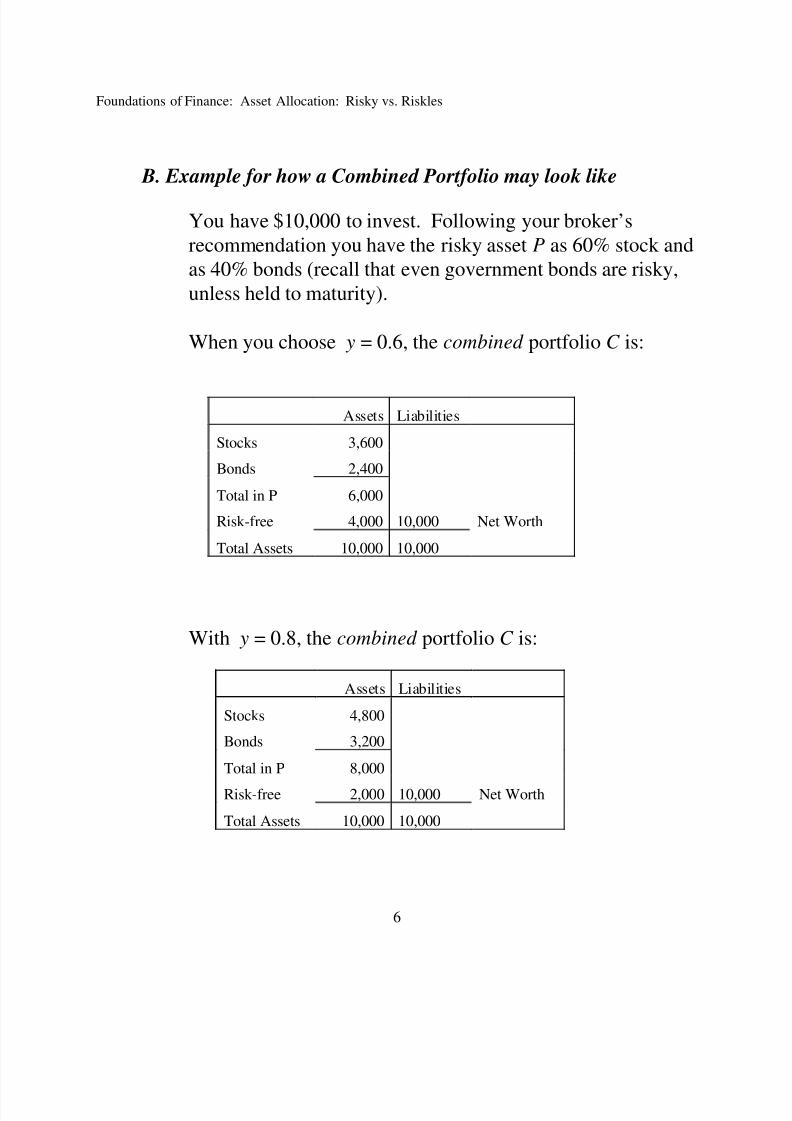
B. Example for how a Combined Portfolio may look like

You have $10,000 to invest. Following your broker’srecommendation you have the risky asset P as 60% stock andas 40% bonds (recall that even government bonds are risky,unless held to maturity).

When you choose y = 0.6, the combined portfolio C is:

With y = 0.8, the combined portfolio C is:

Assets Liabilities

Stocks 3,600

Bonds 2,400

Total in P 6,000

Risk-free 4,000 10,000 Net Worth

Total Assets 10,000 10,000

Assets Liabilities

Stocks 4,800

Bonds 3,200

Total in P 8,000

Risk-free 2,000 10,000 Net Worth

Total Assets 10,000 10,000




7

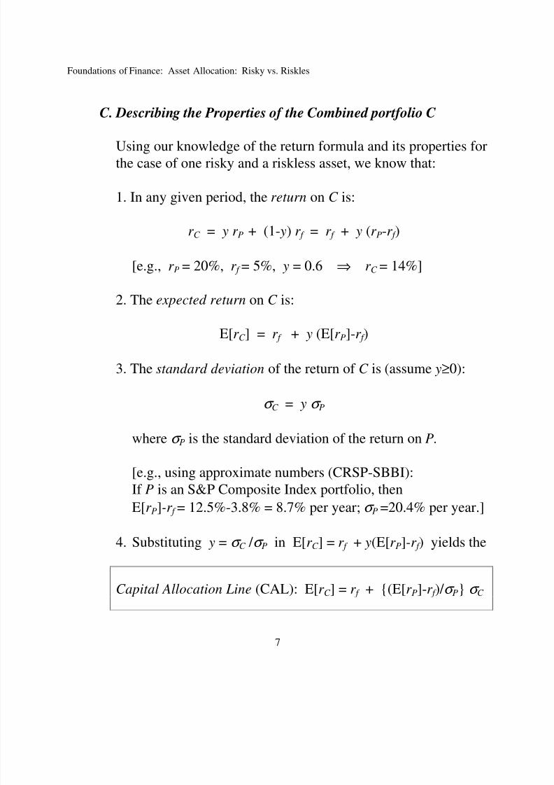
C. Describing the Properties of the Combined portfolio C

Using our knowledge of the return formula and its properties for

the case of one risky and a riskless asset, we know that:

1. In any given period, the return on C is:

r C = y r P + (1- y) r f = r f + y (r P-r f )

[e.g., r P = 20%, r f = 5%, y = 0.6 ⇒ r C = 14%]

2. The expected return on C is:

E[r C ] = r f + y (E[r P]-r f )

3. The standard deviation of the return of C is (assume y≥0):

σ C = y σ P

where σ P is the standard deviation of the return on P.

[e.g., using approximate numbers (CRSP-SBBI):

If P is an S&P Composite Index portfolio, then

E[r P]-r f = 12.5%-3.8% = 8.7% per year; σ P =20.4% per year.]

4. Substituting y = σ C

/ σ P

in E[r C ] = r

f + y(E[r

P]-r

f ) yields the

Capital Allocation Line (CAL): E[r C ] = r f + {(E[r P]-r f )/ σ P} σ C




8

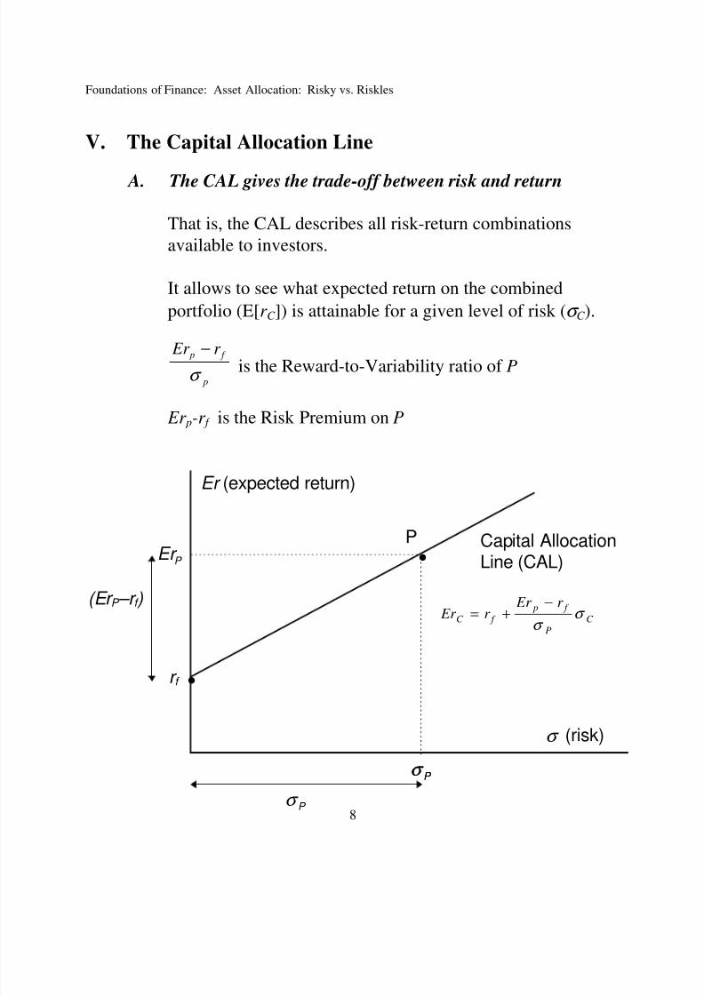
V. The Capital Allocation Line

A. The CAL gives the trade-off between risk and return

That is, the CAL describes all risk-return combinations

available to investors.

It allows to see what expected return on the combined

portfolio (E[r C ]) is attainable for a given level of risk (σ C ).

p

f p r Er

σ

−is the Reward-to-Variability ratio of P

Er p-r f is the Risk Premium on P

σ P

Er P

r f

Er (expected return)

σ (risk)

Capital AllocationLine (CAL)

σ P

σ P

•

•

(Er P –r f )

P

C

P

f p

f C

r Er r Er σ

σ

−+=




9

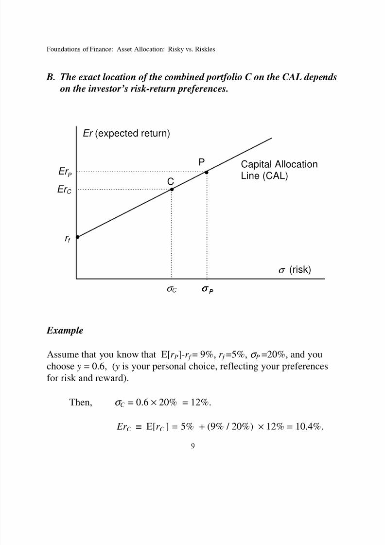
B. The exact location of the combined portfolio C on the CAL depends

on the investor’s risk-return preferences.

Example

Assume that you know that E[r P]-r f = 9%, r f =5%, σ P =20%, and you

choose y = 0.6, ( y is your personal choice, reflecting your preferences

for risk and reward).

Then, σ C = 0.6 × 20% = 12%.

Er C ≡ E[r C ] = 5% + (9% / 20%) × 12% = 10.4%.

σ P

Er P

r f


σ (risk)


σ P σ P

•

•

•

P

C

σ C

Er C




10

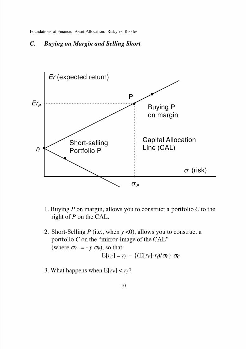
C. Buying on Margin and Selling Short

1. Buying P on margin, allows you to construct a portfolio C to the

right of P on the CAL.

2. Short-Selling P (i.e., when y <0), allows you to construct a

portfolio C on the “mirror-image of the CAL”

(where σ C = - y σ P), so that:

E[r C ] = r f - {(E[r P]-r f )/ σ P} σ C

3. What happens when E[r P] < r f ?

σ P

•

•

Er P

r f


σ (risk)

Short-sellingPortfolio P


σ P

•

P •

Buying Pon margin




11

VI. Portfolio Management:

One Risky Asset and a Riskless Asset A. How would a risk averse investor choose the portfolio

weights for a portfolio consisting solely of the riskless asset

and a given risky asset?

1. For any point on the negative sloped part, a risk averse

individual, with mean-variance preferences, is going to

prefer at least one point on the positive sloped part of the

curve (the one with the same standard deviation and ahigher expected return).

2. If the expected return on a risky asset exceeds the riskless

rate (E[r P] > r f ): an individual forming a portfolio using

only that asset and the riskless asset will not want to short

sell the risky asset (not want y < 0), but the individual may

want to buy it on margin (may want y >1).

3. If the expected return on a risky asset is less than theriskless rate (E[rP] < rf ): an individual forming a portfolio

using only that asset and the riskless asset will want to

short sell the risky asset (will want y <0).

4. The exact weight that the individual wants to hold of the

risky asset depends on her attitudes to risk; different

individuals will choose to hold different amounts of the

risky asset.Who wants to hold positive amounts of both the risky

asset and T-bills (0< y<1)?

Who wants to buy the risky asset on margin ( y>1)?




12

B. Separation Property

The portfolio of risky assets, P, is selected in a separate step,

independent of investors’ attitude for risk.Any (mean-variance) investor, regardless of risk-takingpreferences will prefer the portfolio P with the highest CAL.

Implications of the Separation Property for Portfolio

Management

1. Investment advisers can recommend a single optimalportfolio, with the highest CAL

That’s what they are actually doing in practice, exceptthat different investment advisers may disagree on theportfolio because they differ in their opinion about thefirst and second moments of the risky assets.

2. Investors can use the riskfree asset to adjust investment risk.

The “Cash” in Morgan Stanley’s recommendation isthus used for risk adjustment of the portfolio.

C. The Portfolio Choice Process: Summary so far

So far, we saw two steps to construct your optimal investmentportfolio -- assuming that mean-variance preferences are a gooddescription of your risk profile (e.g., if you are risk averse andreturns are normally distributed):




13

Stage I: Asset Selection

Determine the “best” P available to you in the

mean/standard-deviation space.(For that you need to use the characterization of the return distribution.

So far, we took P as given. The “identity” of P is the subject of thesubsequent lectures on asset selection and equilibrium; this will allowus to better understand how, for example, Morgan Stanley chose theweights of stocks and bonds within P).

Use P to determine the “best” CAL (In our setting it is thesame for all investors that have the same P;

in other words, Asset Selection is an objective procedure).

Stage II: Asset Allocation Find the combined portfolio C that “fits your personal risk profile” as the point on the CAL providing you with the“highest utility.” (C is likely to differ across investors, evenif they have the same P; Asset Allocation is subjective).

Note: In the next lecture we will see how determining the “best P” andthe “best” CAL is done simultaneously.

VII. Additional Readings

The following articles present the evolution of quarterly Asset-Allocation of Wall Street strategists over time, which are the source for our example.

In the context of our discussion, you should view “Stocks” and “Bonds” astwo components of the risky portfolio P, and compare the weight of P to thatof “Cash” (the riskless asset).[As noted, we took the composition of P as given, but we will discuss how toconstruct P in the next lecture. Therefore, you may want to take a look atthese articles again later].

Documents

Asset Allocation Framework