ASSIGNING SHORT-TERM COUNTS TO SEASONAL ADJUSTMENT FACTOR GROUPS

USING SUPPORT VECTOR MACHINES (SVM)

Ioannis Tsapakis, Ph.D., Corresponding Author Texas A&M Transportation Institute (TTI)

Texas A&M University System

1100 N.W. Loop 410, Ste. 400, San Antonio, TX

Tel: (210) 321-1217, Email: i-tsapakis@tamu.edu

William H. Schneider IV, Ph.D., P.E. Department of Civil Engineering

The University of Akron

203 E. Buchtel Avenue, Akron, OH 44325-3901

Phone: +1 (330) 972-2426, Email: whs4@uakron.edu

Word count: 5,498 words text + 6 tables/figures x 250 words (each) = 6,998 words (35 references not

included in the word count)

Submission Date: November 15, 2014

2

ABSTRACT 1 The traditional method of estimating AADT involves several steps, with the most critical being the 2 “assignment” process that involves allocating short-term counts to groups of seasonal adjustment factors 3 (SAFs). The accuracy of AADT estimates highly depends on the assignment step, which is subject to 4 errors stemming from human judgment. Support vector machines (SVM), a supervised learning and 5 statistical method, is employed to construct a series of assignment models that are compared against the 6 traditional method and discriminant analysis (DA) models. Traffic volume data obtained from permanent 7 traffic recorders (PTRs) are used to train and validate the models. The analysis is conducted using SAFs 8 calculated for each direction of travel and separately for two-way traffic. The results revealed that the 9 Gaussian kernel-based SVM model yields the lowest errors improving the AADT accuracy by 65.0% and 10 decreasing the standard deviation of absolute percentage error by 73.7% over the traditional method. 11 Another finding is that the assignment errors of the directional volume-based analysis are lower than 12 those of the total volume-based analysis by 41.8%. The comparison between the two model parameters 13 examined, the ADT and the hourly factors, indicates that the combined use of both parameters in SVM is 14 more effective than when hourly factors are used alone. However, in the case of DA the opposite results 15 are obtained. A possible explanation is that the SVM kernels transfer data from the input space to a 16 feature space providing the ability to effectively assign counts using different types of data within the 17 same model. 18 19

20

Keywords: AADT, Seasonal Adjustment Factors, Permanent Traffic Recorders, Traffic Monitoring, 21 Support Vector Machines22

3

1. INTRODUCTION 23 The annual average daily traffic (AADT) is one of the most commonly used traffic parameters having 24 numerous applications in transportation engineering. AADT expresses the average number of vehicles 25 passing from a specific roadway location within a day throughout a year. The AADT can be directly 26 estimated using data obtained from permanent traffic recorders (PTRs) that measure traffic volumes 27 continuously. The main drawback of PTRs is associated with their high installation, operating, and 28 maintenance cost that does not allow agencies to maintain a large number of PTRs in their transportation 29 system. In order to overcome this constraint, agencies employ portable traffic counters (PTCs) to conduct 30 short-term counts at locations that are not monitored by PTRs. AADT estimates are generated by 31 combining both types of data according to a method, known as the “traditional method”, introduced in 32 1966 by Drusch (1). The first step of this method is widely known as “factoring” and involves calculating 33 seasonal adjustment factors (SAFs) for each PTR. Then, groups of PTRs are created based on their 34 roadway functional class and/or the geographical region where the PTRs are located – this step is known 35 as “grouping.” As part of this step, SAFs are separately estimated for each PTR group. In the third step of 36 the process, called “assignment”, each short-term count is assigned to one of the previously defined 37 groups based on its roadway functional and/or spatial characteristics. Finally, the average daily traffic 38 (ADT) volume of a short-term count is projected to an annual basis by applying an appropriate group 39 SAF. 40

One caveat of the traditional method is that the accuracy of the predictions is subject to 41 cumulative errors inherent within each step (2). Several previous works have examined statistical and 42 non-parametric methods such as neural networks, ordinary least square regression, and principal 43 component analysis to directly estimate the AADT avoiding the intermediate steps of the traditional 44 method (3, 4, 5). Nonetheless, the results of these methods are mixed. Further, developing these methods 45 typically requires advanced statistical software packages, a strong background in econometrics, 46 knowledge of computer programming, and significant amount of data. As a result, a large number of 47 Departments of Transportation (DOTs) still uses variants of the traditional method. 48

Literature reveals that the majority of past studies focus on the factoring and grouping procedures 49 (6). However, prior research has shown that the “assignment” step is the most critical element in the 50 AADT estimation process (7). Potential ineffective allocation of short-term counts to SAF groups may 51 triple the prediction error (8), yet, only a limited number of studies has dealt with improving the 52 assignment procedure (7, 9). Sharma (1993) developed an index of assignment effectiveness to examine 53 how the duration and the frequency of short-term counts affect the AADT estimates (10). The overall 54 effectiveness of the assignment process depended on the magnitude of individual assignment errors (10, 55 11). In a similar study, Sharma (1996) concluded that the duration of short-term counts was of less cause 56 of concern than discrepancies in the assignment procedure (7). Davis and Guan (1996) assigned short-57 term counts to factor groups using Bayesian statistics (12). The authors demonstrated that short-term 58 counts of two-weeks or less produced average estimation errors of ±10%, while shorter counts in duration 59 resulted in average errors of ±20% (12). 60

Li et al. (2006) developed a “fuzzy logic” decision tree that included variables such as hotels, 61 population and the ratio of permanent to seasonal households (13). Li found that the lack of data may 62 produce unreasonable or even poor results, while engineering judgment is necessary (13). Jin et al. (2008) 63 examined a k-nearest neighbor algorithm and used roadway and land use characteristics. The analysis 64 revealed that the AADT accuracy was improved when un-weighted k-nearest neighbor models were used 65 instead of traditional non-cluster methods (14). In 2013, Gastaldi et al. developed a feed-forward back-66 propagation neural network to assign road segments to road groups. The study concluded that the AADT 67 accuracy depends on the period in which short-term counts are taken as well as on land-use and socio-68 economic characteristics (15). 69

According to previous findings and the Traffic Monitoring Guide (2013), the roadway functional 70 classification results in easily identifiable groups of stations that, nonetheless, may be highly 71 heterogeneous (9, 16). The lack of specifications of definable assignment characteristics indicates that 72 there is still room for improvement (14, 15). Previous studies suggest that statistical methods are 73

4

necessary to support the assignment procedure, which is sensitive to human errors stemming from 74 engineering judgment (7, 14, 17, 18). 75 76 1.1 Purpose and Objectives 77 The goal of this study is to reduce the errors associated with the assignment step and improve the AADT 78 accuracy by employing support vector machines (SVM). The selection of SVM over other techniques 79 such as Bayesian analysis (12, 19), decision trees (13), conditional inference forests (20), or k-nearest 80 neighbor methods (14) relies on the fact that SVM is a theoretically superior machine learning 81 methodology with great results in the classification of high-dimensional datasets and has been found 82 competitive with the best machine learning algorithms (21). Additionally, SVM is a viable mathematical 83 data-driven method; is effective in high dimensional spaces and in cases where the number of dimensions 84 is greater than the number of samples; is memory efficient because it uses a subset of training points in 85 the decision function, called support vectors; is versatile due to the different Kernel functions that can be 86 specified for the decision function; and can be used to supplement cluster analysis, which is 87 recommended by the TMG to create PTR groups (16). 88 89 Four objectives have been defined towards the study purpose: 90 91

1. Quantify the performance and compare the effectiveness of two input variables: the ADT and the 92 24 hourly factors of a short-term count. 93

2. Compare the SVM performance using “total volume SAFs” (one SAF for both directions of 94 travel) versus “directional specific SAFs” (one SAF for each direction of travel). 95

3. Develop different SVM and discriminant analysis (DA) models and identify the most effective 96 one. 97

4. Compare the performance of the most effective model against the traditional assignment and the 98 results from past studies. 99

100 The remainder of the paper is organized as follows. The study data are presented in the second 101

section and the methodology is described in section three. The study results are provided and discussed 102 separately for each objective in section four, and conclusions are drawn in the last section. 103 104 2. STUDY DATA 105 The study data include traffic volumes obtained in 2007 and 2008 from 49 PTRs located in the State of 106 Ohio. Similar to data requirements used by previous works (22, 23), in order to minimize the impact of 107 missing data on the final predictions or to avoid additional sources of error introduced by applying data 108 imputation techniques, the researchers filtered out all PTRs that contained less than 310 ADTs within a 109 year. The accuracy of the various models developed in this study is subject to the completeness and 110 quality of this dataset. The AADT and monthly adjustment factors (MAFs) were estimated in accordance 111 with the AASHTO formula (24). 112

In line with prior research findings, the TMG (2013) acknowledges that traffic may vary 113 directionally, thereby SAFs were estimated for two-way traffic volumes and separately for directional 114 volumes (22). This finding is confirmed by an analysis of variance (ANOVA) that revealed statistically 115 significant differences in directional traffic patterns. Following TMG recommendations, after calculating 116 the MAFs, the PTRs were grouped geographically and cluster analysis was applied within each 117 geographical group (16). The 12 MAFs of each station were used to feed the k-means algorithm that was 118 used for clustering (25). 119 120 2.1 Training and Validation Data Sets 121 The PTR data are used as the training data set to create factor groups and as the validation data set from 122 which test short-term counts are generated. All daily counts of all PTRs are treated as test 24-hour counts 123 and are allocated to the previously defined PTR groups. When a short-term count of a station is used as a 124

5

test count, this particular station is left out of the analysis to avoid potential correlations between the PTR 125 and the test count. Then, 365 daily adjustment factors are estimated for each PTR group. Finally, the test 126 count is expanded to an AADT estimate by multiplying the ADT on that particular “test” day with the 127 corresponding group daily adjustment factor. The selection of using 24-hour counts for validation 128 purposes is a conservative scenario because past research has shown that short counts in length are more 129 likely to produce higher prediction errors compared to longer counts (8, 23). 130 131 3. METHODOLOGY 132 This section provides methodological considerations that are presented in five subsections: the traditional 133 method; the model parameters used; the SVM modeling; the DA modeling; and the statistical measures 134 employed to quantify the models’ performance and compare the results. 135 136 3.1 Traditional Method 137 The roadway functional classification was used to create PTR groups and assign them to short-term 138 counts. The main advantages of the traditional method are simplicity, easy interpretation of results, small 139 development effort, and short computing time. Nonetheless, it is limited in scope as the “assignment” is 140 based only on one variable, which cannot effectively reflect the AADT or the traffic patterns of the PTRs 141 (16). Additionally, this method cannot assign short-term counts directionally; hence, only two-way traffic 142 volume SAFs were used in the analysis. 143 144 3.2 Model Parameters 145 In addition to traffic data, as part of the variable selection process the research team initially considered 146 socio-economic, demographic, and land use variables. The results of an exploratory analysis revealed that 147 some data sets had a large percentage of missing values, low spatio-temporal resolution and variability. 148 Due to these limitations, two traffic parameters were selected to develop SVM and DA assignment 149 models: the ADT and a set of 24 hourly factors estimated for a daily count. The two parameters 150 complement each other and can be used interchangeably or in combination to identify segments that 151 exhibit similar traffic patterns. The ADT expresses the magnitude of the daily traffic at a specific location, 152 whereas the 24 hourly factors (Equation 1) capture the traffic variability at a particular site. 153 154

𝐹ℎℎ =𝐴𝐷𝑇

𝐻𝑉ℎℎ, 𝐻𝑉ℎℎ ≠ 0 (1)

155

156

where: 157 HV = hourly volume that corresponds to the hh hour of a day, and 158 hh = 1, 2, 3, …, 24. 159

160 3.3 Support Vector Machines 161 SVM is a supervised learning method that is based on statistical learning theory and is broadly used for 162 classification, regression, and novelty detection purposes (25). SVM was originally introduced in 1992 by 163 Boser et al. and since then, has been employed successfully in many disciplines for handwriting 164 recognition, time-series prediction, database marketing, and many more applications (26). SVM is a 165 kernel-based binary method that can classify two classes, denoted as 𝑀, of linear or nonlinear data. 166

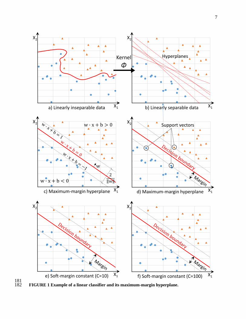
SVM uses a kernel function to map data from the input space (Figure 1a) to a high dimensional 167 feature space (Figure 1b), where a linear solution to a convex optimization problem is found. This 168 solution becomes nonlinear when returned to the input space. Given a training set of input/output pairs, 169 {(𝑥1, 𝑦1), … , (𝑥𝑖, 𝑦𝑖)} ⊂ 𝑋 ∗ ℝ, where 𝑋 denotes the space of the input patterns, the aim is to find the best 170 function 𝑓(𝑥)of the form: 171 172

𝑓(𝑥) = ⟨𝑤, 𝜙(𝑥)⟩ + 𝑏 𝑤𝑖𝑡ℎ 𝑤 ∈ 𝛸, 𝑏 ∈ ℝ (2) 173 174

6

where: 175 𝜙(𝑥)= denotes a nonlinear transformation from the input space to a high dimensional feature space, 176 ⟨∙,∙⟩ = denotes the dot product in 𝑋, 177 𝑤 = the weight vector, and 178 𝑏 = the bias. 179 180

7

181 FIGURE 1 Example of a linear classifier and its maximum-margin hyperplane. 182

Kernel

Φ

Hyperplanes

a) Linearly inseparable data b) Linearly separable data

Support vectors

d) Maximum-margin hyperplane X1

X2

X1

X2

X1

X2

c) Maximum-margin hyperplane X1

X2

f) Soft-margin constant (C=100) X1

X2

e) Soft-margin constant (C=10) X1

X2

8

183 The function 𝑓(𝑥) is a line in two dimensions, a plane in three dimensions, and generally, a 184

hyperplane of the form ⟨𝑤, 𝜙(𝑥)⟩ + 𝑏 = 0 in a high dimensional feature space. The hyperplane divides 185 the space into two regions and the sign of the function 𝑓(𝑥) denotes the side of the hyperplane a point is 186 on (Figure 1c). The boundary between the two regions is called the decision boundary of the classifier and 187 can be either linear or non-linear. The data points that are closer to the decision boundary are called 188 support vectors and their distance from the decision boundary defines the margin of the classifier (Figure 189 1d). The goal of the discriminant function is to maximize the geometric margin 1/‖𝑤‖, which leads to 190 the following constrained optimization problem: 191

192

𝑚𝑖𝑛𝑖𝑚𝑖𝑧𝑒 1

2‖𝑤‖2 (3) 193

194 𝑠𝑢𝑏𝑗𝑒𝑐𝑡 𝑡𝑜: 𝑦𝑖(⟨𝑤, 𝜙(𝑥𝑖)⟩ + 𝑏) ≥ 1 𝑖 = 1, … , 𝑛, (4) 195 196

Data are often not linearly separable, but even if they are, a greater margin can be achieved by 197 allowing the classifier to misclassify some points. To allow errors slack variables 𝜉𝑖 are added leading to 198 the following optimization problem: 199

200

𝑚𝑖𝑛𝑖𝑚𝑖𝑧𝑒 1

2‖w‖2 + 𝐶 ∑ 𝜉𝑖

𝑛𝑖=1 (5) 201

202 𝑠𝑢𝑏𝑗𝑒𝑐𝑡 𝑡𝑜: 𝑦𝑖(⟨𝑤, 𝜙(𝑥𝑖)⟩ + 𝑏) ≥ 1 − 𝜉𝑖, 𝜉𝑖 ≥ 0 (6) 203 204 where: 205 C = constant that sets the relative importance of maximizing the margin and minimizing the amount 206

of slack, 207 𝑦𝑖 = the independent variable, 208 𝑥𝑖 = a 1 ∗ 𝑚 vector of the dependent variables, 𝑖 = 1,2, … , 𝑛, 209 𝑛 = the number of observations, and 210 𝑚 = the number of variables. 211 212 This formulation is known as soft-margin SVM. The effect of the soft-margin constant, C, on the 213

decision boundary is shown in Figures 1e and 1f. A smaller value of C (Figure 1e) allows to ignore points 214 close to the boundary and increases the margin. On the contrary, when C increases (Figure 1f) the dashed 215 lines on the margin are closer to the decision boundary. It is more convenient to solve the optimization 216 problem in its dual formulation, which can be obtained by using Lagrange multipliers. For brevity, the 217 derivations are not covered here but can be found in Smola and Schölkopf (27). The result is the following 218 optimization problem: 219

220

𝑚𝑎𝑥𝑖𝑚𝑖𝑧𝑒{∑ 𝛼𝑖𝑛𝑖=1 − 1/2 ∑ ∑ 𝑦𝑖𝑦𝑗𝑎𝑖𝑎𝑗

𝑛𝑗=1 𝑘(𝑥𝑖, 𝑥𝑗)𝑛

𝑖=1 } (7) 221

222 𝑠𝑢𝑏𝑗𝑒𝑐𝑡 𝑡𝑜 ∑ 𝑦𝑖𝑎𝑖 = 0, 0 ≤ 𝛼𝑖 ≤ 𝐶 𝑛

𝑖=1 (8) 223 224 where: 225 𝛼𝑖 = the Lagrange multipliers, and 226 𝑘 = a kernel function that maps from the input space to feature space. 227 228 The dual formulation leads to an expansion of the weight vector in terms of the input examples: 229 230 𝑤 = ∑ 𝑦𝑖𝑎𝑖𝑥𝑖

𝑛𝑖=1 (9) 231

9

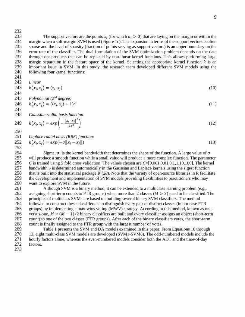
232 The support vectors are the points 𝑥𝑖 (for which 𝑎𝑖 > 0) that are laying on the margin or within the 233

margin when a soft-margin SVM is used (Figure 1c). The expansion in terms of the support vectors is often 234 sparse and the level of sparsity (fraction of points serving as support vectors) is an upper boundary on the 235 error rate of the classifier. The dual formulation of the SVM optimization problem depends on the data 236 through dot products that can be replaced by non-linear kernel functions. This allows performing large 237 margin separation in the feature space of the kernel. Selecting the appropriate kernel function 𝑘 is an 238 important issue in SVΜ. In this study, the research team developed different SVM models using the 239 following four kernel functions: 240 241 Linear 242

𝑘(𝑥𝑖 , 𝑥𝑗) = ⟨𝑥𝑖, 𝑥𝑗⟩ (10) 243

244 Polynomial (2nd degree) 245

𝑘(𝑥𝑖 , 𝑥𝑗) = (⟨𝑥𝑖, 𝑥𝑗⟩ + 1)2 (11) 246

247 Gaussian radial basis function: 248

𝑘(𝑥𝑖 , 𝑥𝑗) = 𝑒𝑥𝑝 (−‖𝑥𝑖−𝑥𝑗‖

2

2𝜎2 ) (12) 249

250 Laplace radial basis (RBF) function: 251

𝑘(𝑥𝑖 , 𝑥𝑗) = 𝑒𝑥𝑝 (−𝜎‖𝑥𝑖 − 𝑥𝑗‖) (13) 252

253 Sigma, 𝜎, is the kernel bandwidth that determines the shape of the function. A large value of 𝜎 254

will produce a smooth function while a small value will produce a more complex function. The parameter 255 C is trained using 5 fold cross validation. The values chosen are C=[0.001,0.01,0.1,1,10,100]. The kernel 256 bandwidth σ is determined automatically in the Gaussian and Laplace kernels using the sigest function 257 that is built into the statistical package R (28). Note that the variety of open-source libraries in R facilitate 258 the development and implementation of SVM models providing flexibilities to practitioners who may 259 want to explore SVM in the future. 260

Although SVM is a binary method, it can be extended to a multiclass learning problem (e.g., 261 assigning short-term counts to PTR groups) when more than 2 classes (𝑀 > 2) need to be classified. The 262 principles of multiclass SVMs are based on building several binary SVM classifiers. The method 263 followed to construct these classifiers is to distinguish every pair of distinct classes (in our case PTR 264 groups) by implementing a max-wins voting (MWV) strategy. According to this method, known as one-265 versus-one, 𝑀 × (𝑀 − 1)/2 binary classifiers are built and every classifier assigns an object (short-term 266 count) to one of the two classes (PTR groups). After each of the binary classifiers votes, the short-term 267 count is finally assigned to the PTR group with the largest number of votes. 268

Table 1 presents the SVM and DA models examined in this paper. From Equations 10 through 269 13, eight multi-class SVM models are developed (SVM1-SVM8). The odd-numbered models include the 270 hourly factors alone, whereas the even-numbered models consider both the ADT and the time-of-day 271 factors. 272 273

10

TABLE 1 Description of SVM and DA Models 274 275

Model Kernel Function Model Variables

SVM1 Linear Fhh

SVM2 Linear ADT, Fhh

SVM3 Polynomial Fhh

SVM4 Polynomial ADT, Fhh

SVM5 Gaussian Fhh

SVM6 Gaussian ADT, Fhh

SVM7 Laplace Fhh

SVM8 Laplace ADT, Fhh

DA9 – Fhh

DA10 – ADT, Fhh

276 3.4 Discriminant Analysis 277 DA is a statistical method that has been used in numerous efforts to assign individual objects to groups of 278 known characteristics (29, 30). The concept behind discriminant analysis includes the creation of 279 discriminant functions that are linear combinations of a test set of independent variables. The functions 280 serve as the foundation for assigning objects (short-term counts in this study) into PTR groups of known 281 monthly traffic patterns. The first function maximizes the distance between the groups. This process is 282 iterative until the functions reach the maximum, which is equal to the minimum value between the 283 (number of groups - 1) and the number of predictors. A set of coefficients is obtained for each group of 284 clusters and a discriminant score is estimated for each discriminant function as follows: 285 286

ppccccc zdzdzddD ,22,11,0, (14) 287

288 where: 289 Dc = standardized score of the discriminant function c, 290 z = variables (ADT and 24 hourly factors), 291 p = number of variables, and 292 dc = discriminant function coefficient. 293

294 The criterion used to assign a count to a PTR group is the largest discriminant score. The 295

classification coefficients dj are estimated from the means of the p predictors and the pooled within-group 296 variance-covariance matrix W. The within-group covariance matrix is calculated by dividing each 297 element in the cross-products matrix by the within-group degrees of freedom. In matrix form: 298

299

Dc = W-1 * Mc (15) 300 301

dco= -0.5 * Dc * Mc (16) 302 303

where: 304 Dc = (dc,1, dc,2, …, dc,p), 305 W-1 = inverse of the within-group variance-covariance matrix, 306 Mc = (Xc,1, Xc,2, …, Xc,p), means for function c on the p variables, and 307

11

dc0 = constant of function c (30). 308 309

The prior probabilities of the PTR groups are assumed to be equal, meaning that members of the 310 test set are not more or less likely to be assigned to a factor group based on the probability of group 311 membership of the training set. The DA method is valid if the short-term count data are independent and 312 the PTR data have a multivariate normal distribution. ANOVA tests are used to measure each variable’s 313 potential before the model development. The contribution of individual predictors and eigenvalues are 314 calculated to assess the magnitude to which the discriminant model fits the data. In all cases, the study 315 data meet the assumptions of the DA methodology. As previously explained, the ADT and the 24 hourly 316 factors are the model predictors used to develop two DA models (Table 1) whose general form is 317 provided in Equations 17 and 18 respectively: 318 319

2424,22,11,0,

1 FdFdFddD ccccc (17)

320

2425,23,12,1,0,

2 FdFdFdADTddD cccccc (18)

321

322 where: 323 Dc = standardized score of the discriminant function c, 324 Fhh = hourly factor that corresponds to the hhth hour of the day, and 325 dc = discriminant function coefficient. 326

327 The comparison of the model results will show whether accounting for all 25 variables is more 328

effective in the assignment process than using the 24 hourly factors alone. Based on previous research 329 findings (31), the variables are selected using the Rao’s V algorithm (Equation 19) that measures the total 330 group separation (32): 331 332

g

z

jjziiz

p

i

p

j

ij XXXXwgnV11 1

*

(19)

333

334

where: 335 nz = sample size of the group z, 336

izX = mean of ith variable in group z, 337

iX = mean of ith variable for all groups combined, 338

jzX = mean of jth variable in group z, 339

jX = mean of jth variable for all groups combined, and 340

*izw = element of the inverse of the within-groups covariance matrix. 341

342 This generalized distance measure applies to any number of groups and measures the separation 343 of group centroids without concerning itself with cohesiveness within a group (32). The larger the 344 differences between group-means the larger the Rao’s V. The DA models were built in SPSS (33). 345 346 3.5 Statistical Validation of Results 347 The majority of past studies validate a limited number of sample short-term counts generated from a small 348 number of stations (11, 14). In this paper, the validation data set consists of 24,900 sample counts that are 349 tested for each SVM and DA model. Validating this extensive dataset is a computationally demanding 350 process, yet, it allows for minimizing random errors and bias caused by outliers. Additionally, the large 351 size of the validation data set better reflects the state of the practice and real data challenges encountered 352

12

by practitioners, who typically have to assign thousands of short-term counts to PTR groups. Lastly, 353 accounting for the entire data population, and not only for carefully selected records that may favor lower 354 prediction errors, allows for determining the realistic model performance under actual and not ideal 355 conditions. 356

Similar to previous research studies (9, 14, 15), the researchers employed three statistical 357 measures to evaluate the performance of the examined methods: the absolute percentage error (APE), 358 Equation 20; the mean absolute percentage error (MAPE), Equation 21, and; the standard deviation of the 359 absolute percentage error (SDAPE), Equation 22. 360 361

100,

,,,

,

Actualv

EstimatedddvActualv

ddvAADT

AADTAADTAPE

(20)

362

q

s Actualv

EstimatedddvActualv

AADT

AADTAADT

qMAPE

1 ,

,,,100

1

(21)

363

1

)(1

2

,

q

MAPEAPE

SDAPE

q

s

ddv

(22)

364

365 where: 366 q = number of test short-term counts, 367 v = ATR index, 368 dd = day of year, 369

ActualvAADT , = actual AADT, and 370

EstimatedddvAADT ,, = estimated AADT. 371

372 Analysis of variance (ANOVA) tests were also conducted to evaluate the statistical significance 373 of the results at a 95% confidence level. 374 375 4. RESULTS 376 The results of the analysis are presented in the following four sections per objective of the study. 377 378 4.1 Objective 1 – Comparison of Model Parameters 379 The first objective involves comparing pairs of models that are based on the same kernel, but include 380 different variables. Figure 2 shows the MAPE of SVM and DA models for both total and directional 381 volume-based SAFs, while Figure 3 illustrates the estimated SDAPE. A visual examination of Figure 2 382 shows that every odd model that accounts for the hourly factors only, results in slightly higher errors than 383 the corresponding even model. For example, in the 2007 total volume-based analysis, SVM3 has a MAPE 384 of 12.1% and SVM4 results in a reduced error of 11.5%. Similar improvements in the MAPE are 385 observed between all pairs of SVM models, for both years, as well as for total and directional specific 386 factors. As part of this comparison, an ANOVA test was carried out to determine whether the individual 387 pairs of models have statistically different means at a 95% confidence interval. The test demonstrated that 388 three out of 16 cases were found to have non-comparable means. These three cases involve SVM1 vs. 389 SVM2 (total volume analysis) and SVM7 vs. SVM8 (directional volume analysis). The highest MAPE 390 improvement (0.7%) occurs between models SVM5 and SVM6 for the year 2008. 391

13

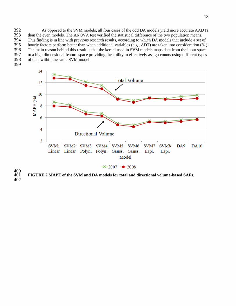
As opposed to the SVM models, all four cases of the odd DA models yield more accurate AADTs 392 than the even models. The ANOVA test verified the statistical difference of the two population means. 393 This finding is in line with previous research results, according to which DA models that include a set of 394 hourly factors perform better than when additional variables (e.g., ADT) are taken into consideration (31). 395 The main reason behind this result is that the kernel used in SVM models maps data from the input space 396 to a high dimensional feature space providing the ability to effectively assign counts using different types 397 of data within the same SVM model. 398 399

400 FIGURE 2 MAPE of the SVM and DA models for total and directional volume-based SAFs. 401 402

14

403

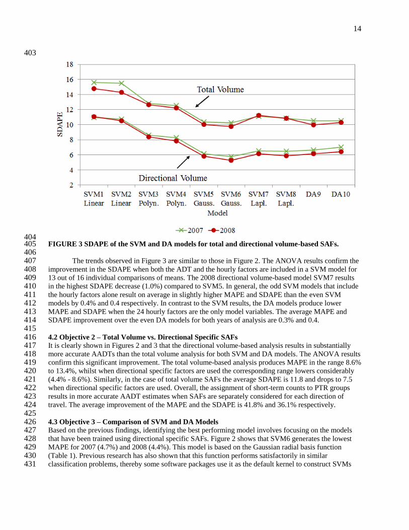
404 FIGURE 3 SDAPE of the SVM and DA models for total and directional volume-based SAFs. 405 406

The trends observed in Figure 3 are similar to those in Figure 2. The ANOVA results confirm the 407 improvement in the SDAPE when both the ADT and the hourly factors are included in a SVM model for 408 13 out of 16 individual comparisons of means. The 2008 directional volume-based model SVM7 results 409 in the highest SDAPE decrease (1.0%) compared to SVM5. In general, the odd SVM models that include 410 the hourly factors alone result on average in slightly higher MAPE and SDAPE than the even SVM 411 models by 0.4% and 0.4 respectively. In contrast to the SVM results, the DA models produce lower 412 MAPE and SDAPE when the 24 hourly factors are the only model variables. The average MAPE and 413 SDAPE improvement over the even DA models for both years of analysis are 0.3% and 0.4. 414 415 4.2 Objective 2 – Total Volume vs. Directional Specific SAFs 416 It is clearly shown in Figures 2 and 3 that the directional volume-based analysis results in substantially 417 more accurate AADTs than the total volume analysis for both SVM and DA models. The ANOVA results 418 confirm this significant improvement. The total volume-based analysis produces MAPE in the range 8.6% 419 to 13.4%, whilst when directional specific factors are used the corresponding range lowers considerably 420 (4.4% - 8.6%). Similarly, in the case of total volume SAFs the average SDAPE is 11.8 and drops to 7.5 421 when directional specific factors are used. Overall, the assignment of short-term counts to PTR groups 422 results in more accurate AADT estimates when SAFs are separately considered for each direction of 423 travel. The average improvement of the MAPE and the SDAPE is 41.8% and 36.1% respectively. 424 425 4.3 Objective 3 – Comparison of SVM and DA Models 426 Based on the previous findings, identifying the best performing model involves focusing on the models 427 that have been trained using directional specific SAFs. Figure 2 shows that SVM6 generates the lowest 428 MAPE for 2007 (4.7%) and 2008 (4.4%). This model is based on the Gaussian radial basis function 429 (Table 1). Previous research has also shown that this function performs satisfactorily in similar 430 classification problems, thereby some software packages use it as the default kernel to construct SVMs 431

15

(28). Similar trends are observed for the SDAPE (Figure 3), which is 5.7 and 5.2 for 2007 and 2008 432 respectively. 433 The Laplace kernel-based model (SVM8) results in the second lowest average MAPE (5.2%) and 434 SDAPE (6.2) among all models examined. The DA models follow, yielding slightly higher average 435 MAPE (5.5%) and SDAPE (6.4). The second degree polynomial-based model (SVM4) did not classify 436 short-term counts at the same degree of precision, producing an average MAPE of 6.5% and average 437 SDAPE of 8.1. Not surprisingly, the linear classifier (SVM2) produced the least accurate AADT 438 estimates. This finding is expected and reveals that the input data can be better classified by using a non-439 linear transformation to a feature space. 440

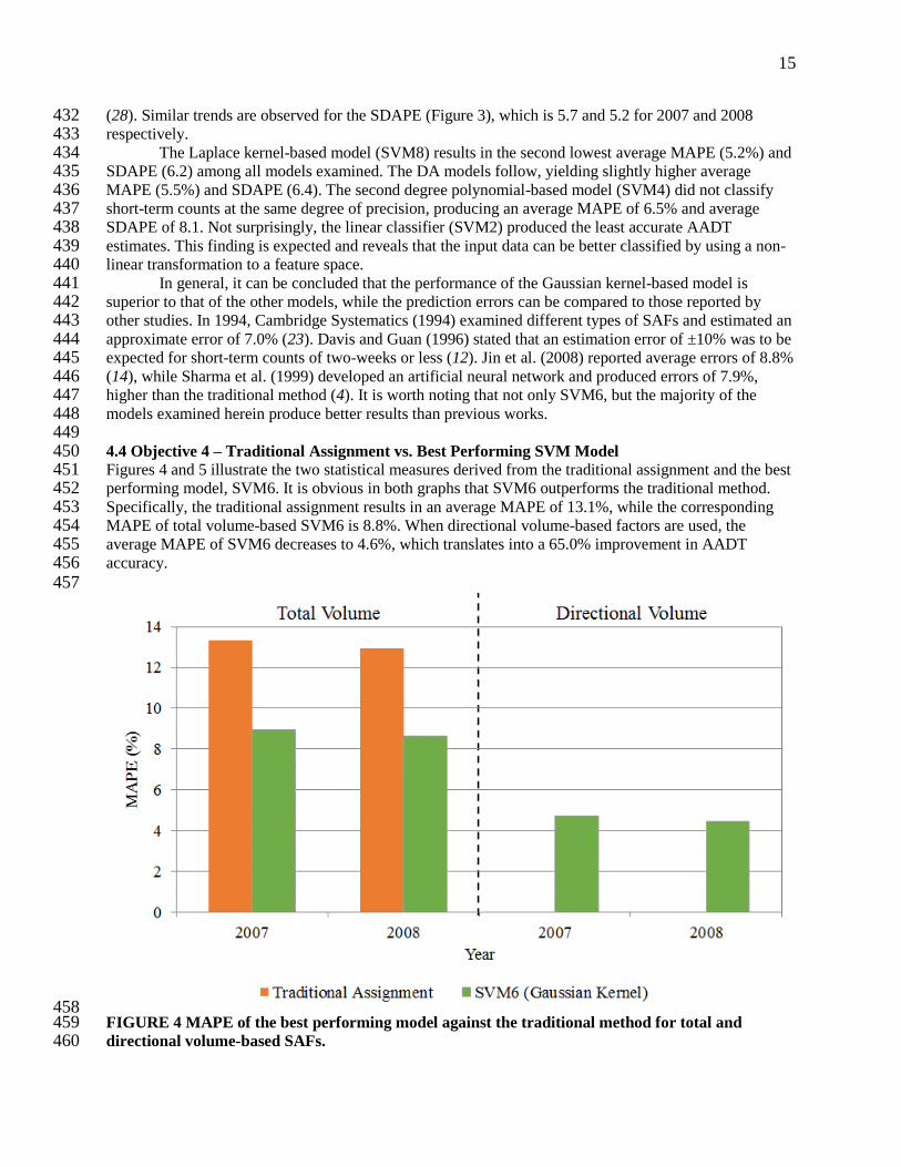
In general, it can be concluded that the performance of the Gaussian kernel-based model is 441 superior to that of the other models, while the prediction errors can be compared to those reported by 442 other studies. In 1994, Cambridge Systematics (1994) examined different types of SAFs and estimated an 443 approximate error of 7.0% (23). Davis and Guan (1996) stated that an estimation error of ±10% was to be 444 expected for short-term counts of two-weeks or less (12). Jin et al. (2008) reported average errors of 8.8% 445 (14), while Sharma et al. (1999) developed an artificial neural network and produced errors of 7.9%, 446 higher than the traditional method (4). It is worth noting that not only SVM6, but the majority of the 447 models examined herein produce better results than previous works. 448 449 4.4 Objective 4 – Traditional Assignment vs. Best Performing SVM Model 450 Figures 4 and 5 illustrate the two statistical measures derived from the traditional assignment and the best 451 performing model, SVM6. It is obvious in both graphs that SVM6 outperforms the traditional method. 452 Specifically, the traditional assignment results in an average MAPE of 13.1%, while the corresponding 453 MAPE of total volume-based SVM6 is 8.8%. When directional volume-based factors are used, the 454 average MAPE of SVM6 decreases to 4.6%, which translates into a 65.0% improvement in AADT 455 accuracy. 456 457

458 FIGURE 4 MAPE of the best performing model against the traditional method for total and 459 directional volume-based SAFs. 460

16

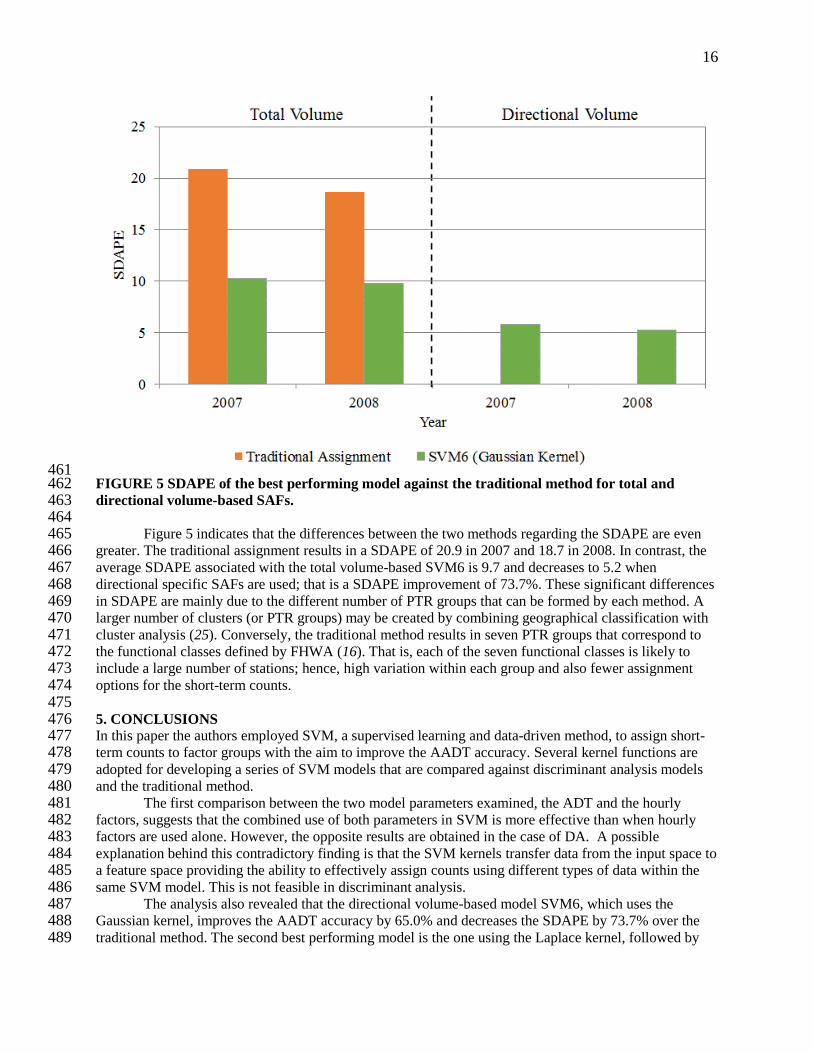
461 FIGURE 5 SDAPE of the best performing model against the traditional method for total and 462 directional volume-based SAFs. 463 464 Figure 5 indicates that the differences between the two methods regarding the SDAPE are even 465 greater. The traditional assignment results in a SDAPE of 20.9 in 2007 and 18.7 in 2008. In contrast, the 466 average SDAPE associated with the total volume-based SVM6 is 9.7 and decreases to 5.2 when 467 directional specific SAFs are used; that is a SDAPE improvement of 73.7%. These significant differences 468 in SDAPE are mainly due to the different number of PTR groups that can be formed by each method. A 469 larger number of clusters (or PTR groups) may be created by combining geographical classification with 470 cluster analysis (25). Conversely, the traditional method results in seven PTR groups that correspond to 471 the functional classes defined by FHWA (16). That is, each of the seven functional classes is likely to 472 include a large number of stations; hence, high variation within each group and also fewer assignment 473 options for the short-term counts. 474 475 5. CONCLUSIONS 476 In this paper the authors employed SVM, a supervised learning and data-driven method, to assign short-477 term counts to factor groups with the aim to improve the AADT accuracy. Several kernel functions are 478 adopted for developing a series of SVM models that are compared against discriminant analysis models 479 and the traditional method. 480

The first comparison between the two model parameters examined, the ADT and the hourly 481 factors, suggests that the combined use of both parameters in SVM is more effective than when hourly 482 factors are used alone. However, the opposite results are obtained in the case of DA. A possible 483 explanation behind this contradictory finding is that the SVM kernels transfer data from the input space to 484 a feature space providing the ability to effectively assign counts using different types of data within the 485 same SVM model. This is not feasible in discriminant analysis. 486

The analysis also revealed that the directional volume-based model SVM6, which uses the 487 Gaussian kernel, improves the AADT accuracy by 65.0% and decreases the SDAPE by 73.7% over the 488 traditional method. The second best performing model is the one using the Laplace kernel, followed by 489

17

the DA model, and the polynomial classifier (SVM4). The least accurate AADT estimates were obtained 490 from the linear classifiers indicating that the input data can be better classified using a non-linear 491 transformation to a feature space. It is noteworthy that the aforementioned errors are conservative because 492 24-hour sample counts were validated. Based on past research findings, the AADT accuracy would be 493 improved if longer duration counts were validated instead (8, 23). Despite this conservative consideration, 494 a comparison with previous studies (4, 12, 14, 23) shows that the majority of the models examined 495 improve the current state of practice. 496 Another conclusion is that the assignment errors of the directional volume-based analysis are 497 lower than those of the total volume-based analysis by 41.8%. This finding is consistent with previous 498 research that suggests time-of-day analyses may be affected by directional distributions (34) and that 499 traffic differs significantly by direction (35). One reason behind this result is that the division of the data 500 set by direction essentially doubles the sample size, which in turn increases the number of assignment 501 options for a short-term count. 502

In general, the plethora of available software packages that contain SVM libraries allows 503 transportation agencies to easily develop and implement SVM. SVM models can be used to estimate 504 truck AADT, minimize human judgment, and supplement cluster analysis that is recommended by 505 FHWA (16). It would be of great interest to validate SVM models using data from other transportation 506 networks that exhibit different geographical and traffic characteristics. The authors are in the process of 507 exploring similar models, accounting for more variables, and examining other variants of the traditional 508 method that are not based solely on functional classification. 509 510 AKNOWLEGMENTS 511 The authors of this paper would like to thank Mr. Dave Gardner, Mr. Tony Manch and Ms. Lindsey 512 Pflum from the Ohio DOT for their valuable help. The contents of this paper reflect the views of the 513 authors and do not necessarily reflect the official views or policies of ODOT or FHWA. 514 515

REFERENCES 516

1. Drusch, R. Estimating Annual Average Daily Traffic from Short-term Traffic Counts. Highway 517 Research Record, No. 118, 1966, pp. 85-95. 518

2. Bodle, R. Evaluation of Rural Coverage Count Duration for Estimating Annual Average Daily 519 Traffic. In Transportation Research Record: Journal of the Transportation Research Board, No. 520 199, Transportation Research Board of the National Academies, Washington, D.C., 1967, pp. 12-521 16. 522

3. Mohamad, D., K. C. Sinha, T. Kuczec, and C. F. Scholer. Annual average daily traffic prediction 523 model for county roads. In Transportation Research Record: Journal of the Transportation 524 Research Board, No. 1617, Transportation Research Board of the National Academies, 525 Washington, D.C., 1998, pp. 69-77. 526

4. Sharma, S. C., P. J. Lingras, F. Xu, and G. X. Liu. Neural networks as alternative to traditional 527 approach of annual average daily traffic estimation from traffic counts. In Transportation 528 Research Record: Journal of the Transportation Research Board, No. 1660, Transportation 529 Research Board of the National Academies, Washington, D.C., 1999, pp. 24-31. 530

5. Seaver, W. L., A. Chatterjee, and M. L. Seaver. Estimation of traffic volume on rural local roads. 531 In Transportation Research Record: Journal of the Transportation Research Board, No. 719, 532 Transportation Research Board of the National Academies, Washington, D.C., 2000, pp. 121-128. 533

6. Gulati, B. M. Precision of AADT Estimates from Short Period Traffic Counts. M.S. thesis. 534 University of Regina, Saskatchewan, Canada, 1995. 535

7. Sharma S. C., B. M. Gulati, and S. N. Rizak. Statewide traffic volume studies and precision of 536 AADT estimates. Journal of Transportation Engineering, 122 (6), 1996, pp. 430-439. 537

18

8. Davis, G. A. Estimation Theory Approaches to Monitoring and Updating Average Annual Daily 538 Traffic. Office of Research Administration, Minnesota Department of Transportation, St. Paul, 539 1996. 540

9. Aunet, B. Wisconsin’s Approach to Variation in Traffic Data. North American Travel 541 Monitoring Exhibition and Conference (NATMEC), Wisconsin Department of Transportation, 542 National Transportation Library, 2000. 543

10. Sharma, S. C., and R. R. Allipuram. Duration and Frequency of Seasonal Traffic Counts. Journal 544 of Transportation Engineering, 119 (3), 1993, pp. 345-359. 545

11. Sharma, S. C., and Y. Leng. Seasonal Traffic Counts for a Precise Estimation of AADT. Institute 546 of Transportation Engineers, 64 (9), 1994, pp. 21-28. 547

12. Davis, G. A., and Y. Guan. Bayesian Assignment of Coverage Count Locations to Factor Groups 548 and Estimation of Mean Daily Traffic. In Transportation Research Record: Journal of the 549 Transportation Research Board, No. 1542, Transportation Research Board of the National 550 Academies, Washington, D.C., 1996, pp. 30-37. 551

13. Li, M. T., F. Zhao, and L. F. Chow. Assignment of Seasonal Factor Categories to Urban 552 Coverage Count Stations Using a Fuzzy Decision Tree. Journal of Transportation Engineering 553 132 (8), 2006, pp. 654-662. 554

14. Jin, L., C. Xu, and J. D. Fricker. Comparison of Annual Average Daily Traffic Estimates: 555 Traditional Factor, Statistical, Artificial Neural Network, and Fuzzy Basis Neural Network 556 Approach. Transportation Research Board 87th Annual Meeting, TRB, Washington, D.C., 2008. 557

15. Gastaldi, M., R. Rossi, G. Gecchele, and L.D. Lucia. Annual Average Daily Traffic Estimation 558 from Seasonal Traffic Counts. Procedia – Social and Behavioral Sciences, 87, October 2013, pp. 559 279-291. 560

16. Federal Highway Administration. Traffic Monitoring Guide, Office of Highway Policy 561 Information. Washington, D.C., September 2013. 562

17. Zhao, F., M. T. Li, and L. F. Chow. Alternatives for Estimating Seasonal Factors on Rural and 563 Urban Roads in Florida. Final Report. Research Center, Florida International University, Florida 564 Department of Transportation, 2004. 565

18. Ritchie, S., and M. Hallenbeck. Evaluation of a Statewide Highway Data Collection Program. 566 Transportation Research Record: Journal of the Transportation Research Board, No. 1090, 567 Transportation Research Board of the National Academies, Washington, D.C., 1986, pp. 27-35. 568

19. Foreman, L.A; A.F.M. Smith, and I.W. Evett. Bayesian analysis of deoxyribonucleic acid 569 profiling data in forensic identification applications (with discussion). Journal of the Royal 570 Statistical Society, Series A, 160, 1997, pp. 429-469. 571

20. Das A., Abdel-Aty M. and A. Pande. Using Conditional Inference Forests to Identify the Factors 572 Affecting Crash Severity on Arterial Corridors, Journal of Safety Research, Vol. 40, 2009, pp. 573 317-327. 574

21. Tzotsos, A., and D. Argialas. Object-Based Image Analysis, Lecture Notes in Geoinformation 575 and Cartography, Springer Berlin Heidelberg, 2008, pp. 663-677. 576

22. Tsapakis, I., W. H. Schneider, A. Nichols, and J. Haworth. Alternatives in Assigning Coverage 577 Counts to Factor Groupings for a Precise Estimation of Annual Average Daily Traffic. Journal of 578 Advanced Transportation, March 2012. 579

23. Cambridge Systematics and Science Application International Corporation. Use of Data from 580 Continuous Monitoring Sites. Prepared for FHWA, Volume I and II, Documentation, FHWA, 581 August 1994. 582

24. AASHTO. Joint Task Force on Traffic Monitoring of the AASHTO Highway Subcommittee on 583 Traffic Engineering Guidelines for Traffic Data Programs, Washington D.C., 1992. 584

25. Tsapakis, I., W.H. Schneider, and A.P. Nichols. Improving the Estimation of Total and 585 Directional-Based Heavy-Duty Vehicle Annual Average Daily Traffic (AADT). Transportation 586 Planning and Technology; Vol. 34, No. 2, 2011, pp. 155–166. 587

19

26. Boser, B., I. Guyon, and V. Vapnik. A Training Algorithm for Optimal Margin Classifiers, 5th 588 Annual Workshop on Computational Learning Theory, Pittsburgh, ACM 1992, pp. 144–152. 589

27. Smola, A.J., and B. Schölkopf. A Tutorial on Support Vector Regression. Statistics and 590 Computing, Vol. 14, No. 3, 2004, pp.199–222. 591

28. Karatzoglou, A., A. Smola, K. Hornik, and A. Zeileis. Kernlab-An S4 Package for Kernel 592 Methods in R. Journal of Statistical Software. Vol. 11, No. 9, 2004, pp. 1-20. 593

29. Olden, N. D., and D. A. Jackson. A comparison of Statistical Approaches for Modeling Fish 594 Species Distributions. Freshwater Biology, Vol. 47, 2002, pp. 1976–1995. 595

30. Walker, P. Sexing Skulls Using Discriminant Function Analysis of Visually Assessed Traits. 596 American Journal of Physical Anthropology, Vol. 136, 2008, pp. 39–50. 597

31. Tsapakis, I., W. H. Schneider, A. Bolbol, and A. Skarlatidou. Discriminant Analysis for 598 Assigning Short-Term Counts to Seasonal Adjustment Factor Groupings. Transportation 599 Research Record: Journal of the Transportation Research Board, No. 2256, Transportation 600 Research Board of the National Academies, Washington, D.C., 2011, pp. 112-119. 601

32. Rao, C.R. Linear Statistical Inference and Its Applications, 2nd edition, New York: Wiley, 1973. 602 33. Statistical Package for the Social Sciences. SPSS Tutorial. SPSS for Windows, Version 16.0, 603

Chicago IL, SPSS Inc. 604 34. Hallenbeck, M., M. Rice, B. Smith, C. J. Cornell-Martinez, and J. Wilkinson. Vehicle Volume 605

Distributions by Classification. Final Report, Washington State Transportation Center & 606 Chaparral Systems Corporation, July 1997. 607

35. Wright, T., P. S. Hu, J. Young, and A. Lu. Variability in Traffic Monitoring Data. Final Summary 608 Report, Oak Ridge National Laboratory, 1997. 609

610