Associate Professor: C. H.LIAO

Contents: 4.1 Introduction 1444.2 Nonlinear Oscillations 1464.3 Phase Diagrams for Nonlinear Systems

1504.4 Plane Pendulum 1554.5 Jumps, Hysteresis, and Phase Lags 1604.6 Chaos in a Pendulum 1634.7 Mapping 1694.8 Chaos Identification 174

4.1 Introduction

When pressed to divulge greater detail, however, nature insists of being nonlinear; examples are the flapping of a flag in the wind, the dripping of a leaky water faucet, and the oscillations of a double pendulum.

The famous French mathematician Pierre Simon de Laplace espoused the view that if we knew the position and velocities of all the particles in the universe, then we would know the future for all time.

Much of nature seems to be chaotic. In this case, we refer to deterministic chaos, as opposed to randomness, to be the motion of a system whose time evolution has a sensitive dependence on initial conditions.

Sol.:

However, if it had been necessary to stretch each spring a distance d to attach it to the mass when at the equilibrium position, then we would find for the force

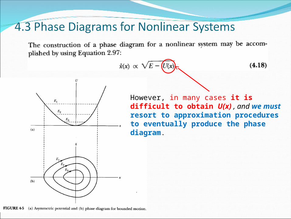
However, in many cases it is difficult to obtain U(x) , and we must resort to approximation procedures to eventually produce the phase diagram.

By referring to the phase paths for the potentials shown in Figures 4-5 and 4-6, we can rapidly construct a phase diagram for any arbitrary potential

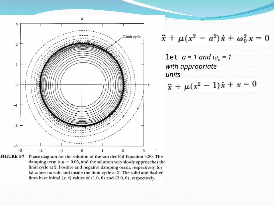
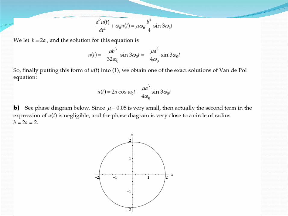
let a = 1 and ωo = 1 with appropriate units

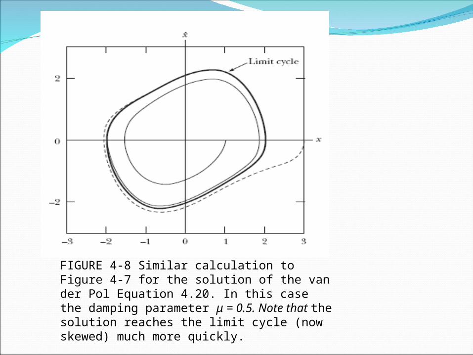
FIGURE 4-8 Similar calculation to Figure 4-7 for the solution of the van der Pol Equation 4.20. In this case the damping parameter μ = 0.5. Note that the solution reaches the limit cycle (now skewed) much more quickly.

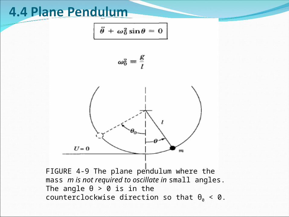
FIGURE 4-9 The plane pendulum where the mass m is not required to oscillate in small angles. The angle θ > 0 is in the counterclockwise direction so that θ0 < 0.

FIGURE 4-10 The component of the force, F(θ), and its associated potential that acts on the plane pendulum. Notice that the force is nonlinear.

T + U = E = constant

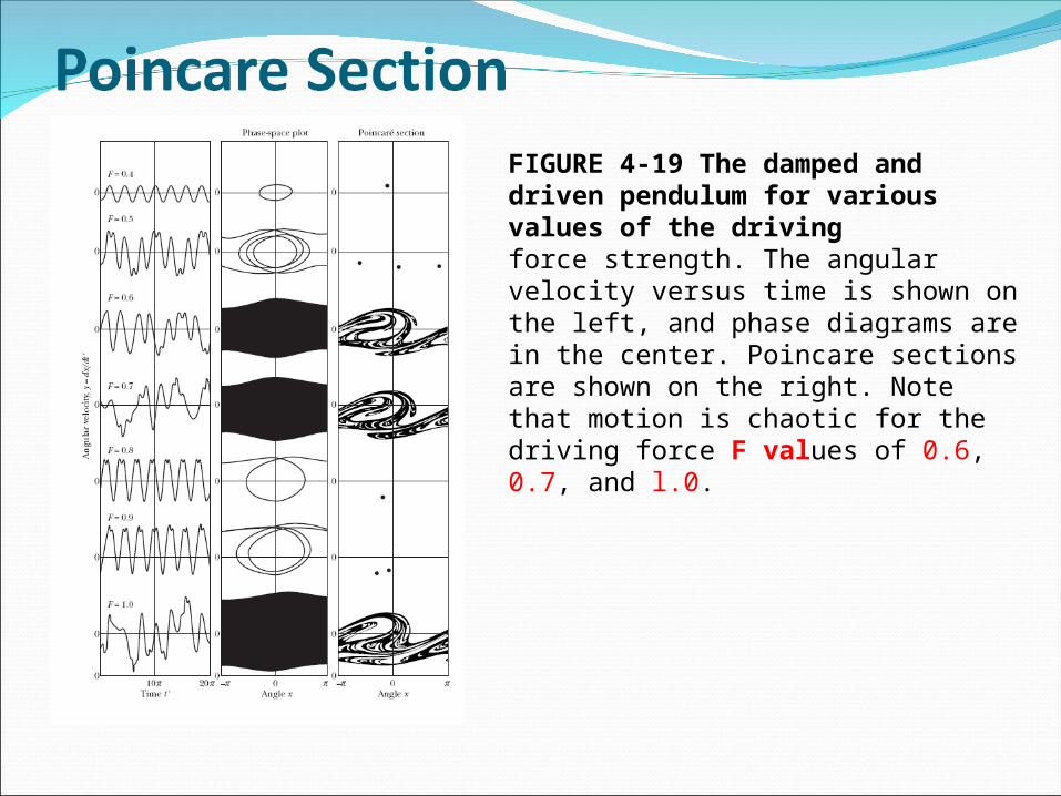
FIGURE 4-19 The damped and driven pendulum for various values of the drivingforce strength. The angular velocity versus time is shown on the left, and phase diagrams are in the center. Poincare sections are shown on the right. Note that motion is chaotic for the driving force F values of 0.6, 0.7, and l.0.

Thanks for your attention.

Problem discussion.Problem:4-2, 4-4, 4-9, 4-13, 4-17, 4-20, 4-24

P.S. : # This is an optional problem.