ASTATIC Documentation - Zonge International · ASTATIC v3.70 documentation page 5 Geographic coordinates are specified as eastings, northings and elevation rather than x, y, z to

ASTATIC v3.70 documentation page 1

ASTATIC Documentation Version 3.70 July 24, 2014

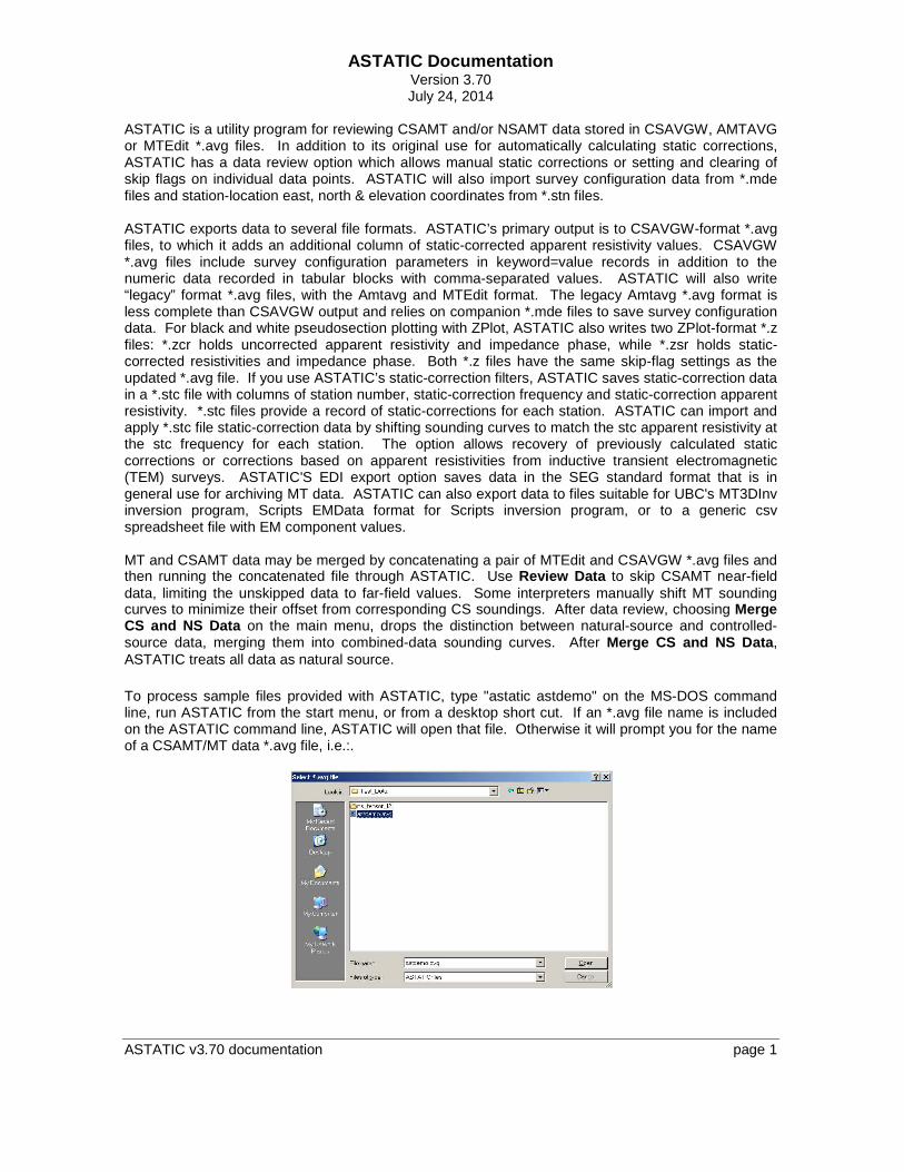
ASTATIC is a utility program for reviewing CSAMT and/or NSAMT data stored in CSAVGW, AMTAVG or MTEdit *.avg files. In addition to its original use for automatically calculating static corrections, ASTATIC has a data review option which allows manual static corrections or setting and clearing of skip flags on individual data points. ASTATIC will also import survey configuration data from *.mde files and station-location east, north & elevation coordinates from *.stn files. ASTATIC exports data to several file formats. ASTATIC’s primary output is to CSAVGW-format *.avg files, to which it adds an additional column of static-corrected apparent resistivity values. CSAVGW *.avg files include survey configuration parameters in keyword=value records in addition to the numeric data recorded in tabular blocks with comma-separated values. ASTATIC will also write “legacy” format *.avg files, with the Amtavg and MTEdit format. The legacy Amtavg *.avg format is less complete than CSAVGW output and relies on companion *.mde files to save survey configuration data. For black and white pseudosection plotting with ZPlot, ASTATIC also writes two ZPlot-format *.z files: *.zcr holds uncorrected apparent resistivity and impedance phase, while *.zsr holds static-corrected resistivities and impedance phase. Both *.z files have the same skip-flag settings as the updated *.avg file. If you use ASTATIC’s static-correction filters, ASTATIC saves static-correction data in a *.stc file with columns of station number, static-correction frequency and static-correction apparent resistivity. *.stc files provide a record of static-corrections for each station. ASTATIC can import and apply *.stc file static-correction data by shifting sounding curves to match the stc apparent resistivity at the stc frequency for each station. The option allows recovery of previously calculated static corrections or corrections based on apparent resistivities from inductive transient electromagnetic (TEM) surveys. ASTATIC'S EDI export option saves data in the SEG standard format that is in general use for archiving MT data. ASTATIC can also export data to files suitable for UBC's MT3DInv inversion program, Scripts EMData format for Scripts inversion program, or to a generic csv spreadsheet file with EM component values. MT and CSAMT data may be merged by concatenating a pair of MTEdit and CSAVGW *.avg files and then running the concatenated file through ASTATIC. Use Review Data to skip CSAMT near-field data, limiting the unskipped data to far-field values. Some interpreters manually shift MT sounding curves to minimize their offset from corresponding CS soundings. After data review, choosing Merge CS and NS Data on the main menu, drops the distinction between natural-source and controlled-source data, merging them into combined-data sounding curves. After Merge CS and NS Data, ASTATIC treats all data as natural source. To process sample files provided with ASTATIC, type "astatic astdemo" on the MS-DOS command line, run ASTATIC from the start menu, or from a desktop short cut. If an *.avg file name is included on the ASTATIC command line, ASTATIC will open that file. Otherwise it will prompt you for the name of a CSAMT/MT data *.avg file, i.e.:.


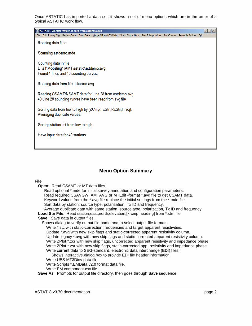
Once ASTATIC has imported a data set, it shows a set of menu options which are in the order of a typical ASTATIC work flow.

Menu Option Summary File Open: Read CSAMT or MT data files Read optional *.mde for initial survey annotation and configuration parameters. Read required CSAVGW, AMTAVG or MTEdit -format *.avg file to get CSAMT data. Keyword values from the *.avg file replace the initial settings from the *.mde file. Sort data by station, source type, polarization, Tx ID and frequency. Average duplicate data with same station, source type, polarization, Tx ID and frequency Load Stn File: Read station,east,north,elevation,[x-cmp heading] from *.stn file Save: Save data in output files. Shows dialog to verify output file name and to select output file formats. Write *.stc with static-correction frequencies and target apparent resistivities. Update *.avg with new skip flags and static-corrected apparent resistivity column. Update legacy *.avg with new skip flags and static-corrected apparent resistivity column. Write ZPlot *.zcr with new skip flags, uncorrected apparent resistivity and impedance phase. Write ZPlot *.zsr with new skip flags, static-corrected app. resistivity and impedance phase. Write current data to SEG-standard, electronic data interchange (EDI) files. Shows interactive dialog box to provide EDI file header information. Write UBS MT3Dinv data file. Write Scripts *.EMData v2.0 format data file. Write EM component csv file. Save As: Prompts for output file directory, then goes through Save sequence


Menu Option Summary (continued) Edit Survey Cfg: Review survey annotation and configuration parameters. Optionally import station location and possibly EM component orientation values from a *.stn file. Review Data: Review data pseudosections or log-log sounding-curve plots, set skip flags on bad-data points, manually shift curves. Drop Data Auto Skip: set skip flags with data error thresholds Drop skipped data: delete skip-flagged data points Window Data and Drop: window data with data-parameter ranges Merge NS and CS data: Drops distinction between NS and CS data, making everything NS (natural source) Sort data by station, polarization and frequency. Average duplicate data with same station, polarization and frequency. Static Corrections: Static correction options. Stack Static Corrections: Set uncorrected apparent resistivities to static corrected values, to allow application of a second static-correction procedure. Use *.STC File: Read static-correction frequency and target resistivity from *.stc file. Trimmed Moving Average: Apply a five-point trimmed-moving-average filter at a single static-correction frequency. Fixed-Length Moving Average: Use a fixed-length-moving-average filter at a single static-correction frequency. Adaptive Moving Average: Use an adaptive-moving-average filter at a single static-correction frequency. D+ Interpolation: Interpolate data to equal-interval frequencies using a D+ model fit. Plot Curves: Plot Apparent Resistivity, Impedance Phase, |E| and |B| versus frequency. Remedial Action |Z| from smoothed phase(Z): Estimate apparent resistivity sounding curves from integration of phase(Z) versus frequency. Robust 2D Smoothing Filter: Apply an experimental two-dimensional smoothing to apparent resistivity pseudosection values. Smoothing is not recommended for routine data processing. Correct Capacitive Coupling: Reduce capacitive coupling effects due to data acquisition with contact resistance (kohms)*setup wire length (km) > 2 Rescale station numbers: Rescale client station numbers with offset and linear multiplier Shift Ey stations: Apply offset to Ey gdp station numbers Review CSAMT H Data: Review CSAMT H-field data pseudosections Exit: Exit ASTATIC


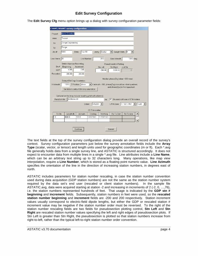
Edit Survey Configuration The Edit Survey Cfg menu option brings up a dialog with survey configuration parameter fields:

The text fields at the top of the survey configuration dialog provide an overall record of the survey’s context. Survey configuration parameters just below the survey annotation fields include the Array Type (scalar, vector, or tensor) and length units used for geographic coordinates (m or ft). Each *.avg file generally holds data from a single survey line, and ASTATIC is structured accordingly. It does not expect to encounter data from multiple lines in a single *.avg file. Line attributes include a Line Name, which can be an arbitrary text string up to 32 characters long. Many operations, like map view interpolation, require a Line Number, which is stored as a floating point numeric value. Line Azimuth specifies the orientation of the line in the direction of increasing station numbers, in degrees east of north. ASTATIC includes parameters for station number rescaling, in case the station number convention used during data acquisition (GDP station numbers) are not the same as the station number system required by the data set’s end user (rescaled or client station numbers). In the sample file ASTATIC.avg, data were acquired starting at station -2 and increasing in increments of 2 (-2, 0, …,76), i.e. the station numbers represented hundreds of feet. That usage is indicated by the GDP stn # beginning and increment fields. Subsequently, station numbers in feet were used, so the rescaled station number beginning and increment fields are -200 and 200 respectively. Station increment values usually correspond to electric-field dipole lengths, but either the GDP or rescaled station # increment value may be negative if the station number order must be reversed. To the right of the station number rescaling fields are two fields for pseudosection plotting control, Stn Left and Stn Right are rescaled station number values specifying the left and right edges of pseudosection plots. If Stn Left is greater than Stn Right, the pseudosection is plotted so that station numbers increase from right-to-left, rather than the typical left-to-right station number order convention.


Geographic coordinates are specified as eastings, northings and elevation rather than x, y, z to keep them distinct from the (x,y,z) coordinate system used to measure electromagnetic field components. The EM Ex and Hx field components are usually oriented along line, so ASTATIC uses line azimuth for its default EM positive X azimuth value. EM x and y components are nearly always horizontal for CSAMT/NSAMT surveys and ASTATIC makes that assumption by default. Zonge data processing and modeling programs require the use of a right-handed x,y,z coordinate system, but the z component may be positive up or positive down. Select z positive if the positive y- component azimuth is 90 degrees counter-clockwise of the positive x-component azimuth in map view. Alternatively, choosing z positive down implies that the positive y EM component is 90 degrees clockwise of positive x component in map view. Choosing z positive up or down also has consequences for the phase of Ex/Hy and Ey/Hx. For the e+iwt time convention used by Zonge, phase(Ex/Hy) should be in the third quadrant and phase(Ey/Hx) should be in the first quadrant for z positive up. First quadrant means phase values between 0 and 1570 mrad, while third quadrant means -3141 to -1570 mrad. If an EM x,y,z component coordinate system with z positive down is used, then phase(Ex/Hy) should be in the first quadrant and phase(Ey/Hx) should be in the third quadrant. Getting the polarity of the EM components oriented in a consistent right-handed x,y,z coordinate system is critical for tensor measurements, but is less important for scalar or vector data acquisition. ASTATIC makes a default estimate of z positive up or down by looking at the median values of phase(Ex/Hy) and phase(Ey/Hx). It also shows those median phase values as text in the survey configuration dialog. If phase(Ex/Hy) and phase(Ey/Hx) are in the same quadrant, the data have been acquired with inconsistent (x,y,z) E and H component polarities and the problem should be fixed before proceeding with the analysis of tensor data sets. Selecting the Set data to default EM cmp orientation button with a mouse click, sets heading, pitch and roll values for all stations with heading = x azimuth, pitch = 0, and roll = 0 for z+ up or 180 for z+ down. Heading, pitch and roll values specify the orientation of x,y,z EM components relative to east, north and up. If east, north, elevation coordinate values are UTM meters, which is true more often than not, checking the Stn east, north, are in UTM meters check box makes two additional fields visible. Datum and UTM Zone. The datum applies to both lat,lon and UTM coordinates. Knowing the UTM zone allows a transform from UTM east,north coordinates to recover lat,lon values. .


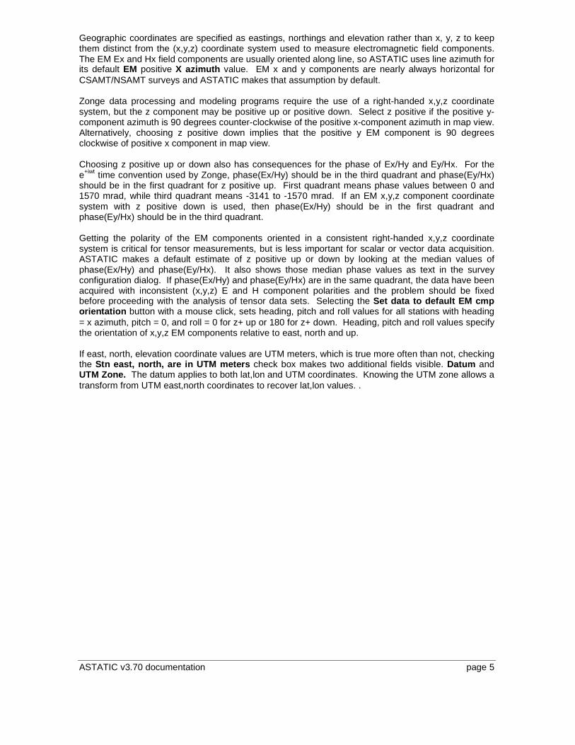
Geographic coordinates for each station may be added to the data set by clicking on the Read stn file button. If ASTATIC can’t find the specified *.stn file, it will show an Open File prompt to allow browsing to a different folder or selection of a different file. Once a *.stn file is selected, ASTATIC reads the *.stn file's values and displays station locations in map view.

Station locations are indicated by dots with a small arrow indicating the orientation of the EM x component. Station elevations are indicated by dot color. A color bar on the right edge of the plot shows the relationship between color and elevation. Text annotation in the lower-left corner of the station location plot reports station location statistics. The sample file astdemo.stn includes the required *.stn file columns of station, easting, northing and elevation and optional columns of heading, pitch and roll. Heading, pitch and roll columns are not required in *.stn files, but may be included if it is necessary to specify different EM component orientations for some stations. The station location map display will close after 30 seconds or at the first mouse-button or key press. The bottom of the CSAMT/NSAMT survey configuration dialog includes a field for the parameters of one to eight controlled-source transmitters. Each transmitter is identified by the GDP Tx station number, and ASTATIC prompts for the additional information specifying the transmitter’s length, orientation and center coordinates. If receiver station coordinates have been imported from a *.stn file by either CSAVGW or by ASTATIC, ASTATIC will show the distance and azimuth between the average receiver station easting and northing and Tx center. The distance and azimuth provide a quick check on location coordinate values. Clicking on the Continue button saves any changes made to the survey configuration and returns control to the main menu, while the Cancel button drops any changes and restores the original values before returning to ASTATIC's main menu.


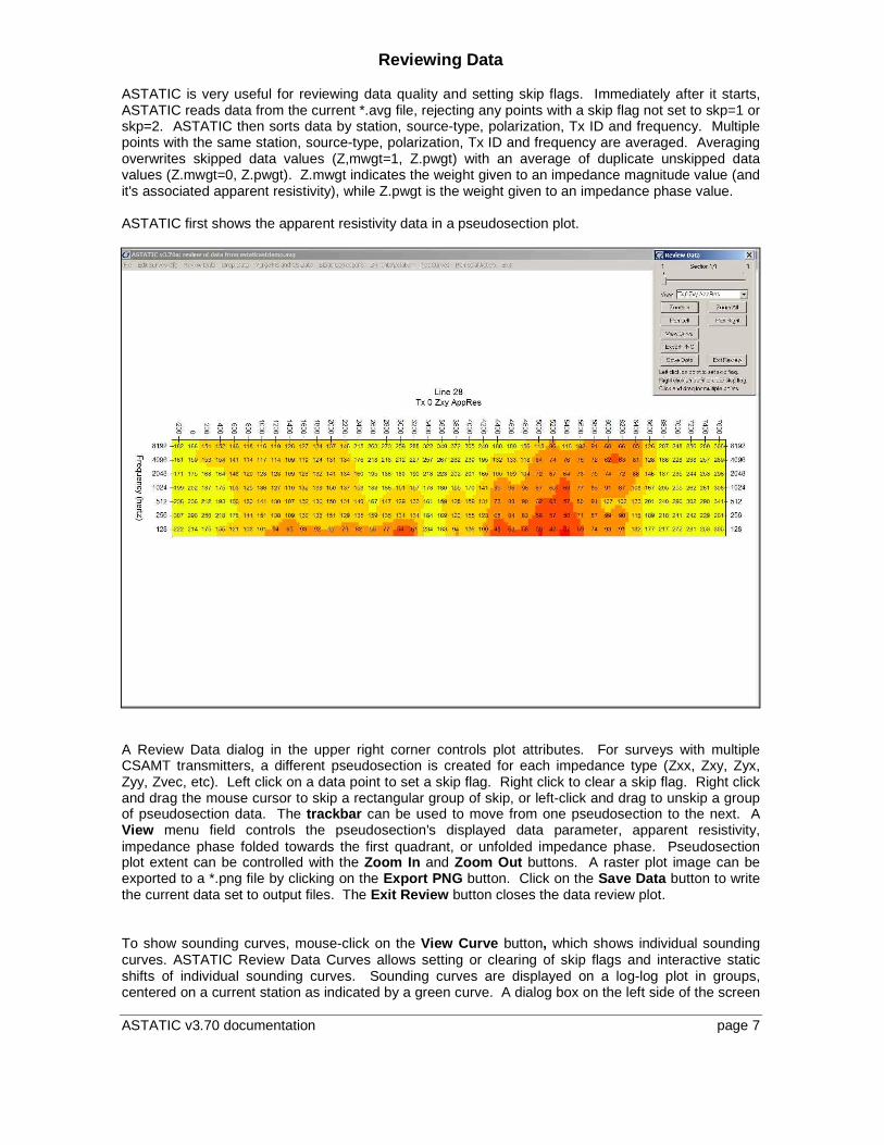
Reviewing Data ASTATIC is very useful for reviewing data quality and setting skip flags. Immediately after it starts, ASTATIC reads data from the current *.avg file, rejecting any points with a skip flag not set to skp=1 or skp=2. ASTATIC then sorts data by station, source-type, polarization, Tx ID and frequency. Multiple points with the same station, source-type, polarization, Tx ID and frequency are averaged. Averaging overwrites skipped data values (Z,mwgt=1, Z.pwgt) with an average of duplicate unskipped data values (Z.mwgt=0, Z.pwgt). Z.mwgt indicates the weight given to an impedance magnitude value (and it's associated apparent resistivity), while Z.pwgt is the weight given to an impedance phase value. ASTATIC first shows the apparent resistivity data in a pseudosection plot.

A Review Data dialog in the upper right corner controls plot attributes. For surveys with multiple CSAMT transmitters, a different pseudosection is created for each impedance type (Zxx, Zxy, Zyx, Zyy, Zvec, etc). Left click on a data point to set a skip flag. Right click to clear a skip flag. Right click and drag the mouse cursor to skip a rectangular group of skip, or left-click and drag to unskip a group of pseudosection data. The trackbar can be used to move from one pseudosection to the next. A View menu field controls the pseudosection's displayed data parameter, apparent resistivity, impedance phase folded towards the first quadrant, or unfolded impedance phase. Pseudosection plot extent can be controlled with the Zoom In and Zoom Out buttons. A raster plot image can be exported to a *.png file by clicking on the Export PNG button. Click on the Save Data button to write the current data set to output files. The Exit Review button closes the data review plot. To show sounding curves, mouse-click on the View Curve button, which shows individual sounding curves. ASTATIC Review Data Curves allows setting or clearing of skip flags and interactive static shifts of individual sounding curves. Sounding curves are displayed on a log-log plot in groups, centered on a current station as indicated by a green curve. A dialog box on the left side of the screen


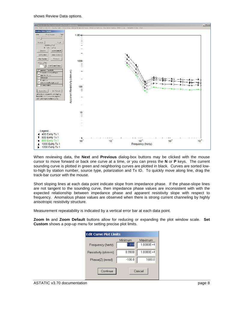
shows Review Data options.

When reviewing data, the Next and Previous dialog-box buttons may be clicked with the mouse cursor to move forward or back one curve at a time, or you can press the N or P keys. The current sounding curve is plotted in green and neighboring curves are plotted in black. Curves are sorted low-to-high by station number, source type, polarization and Tx ID. To quickly move along line, drag the track-bar cursor with the mouse. Short sloping lines at each data point indicate slope from impedance phase. If the phase-slope lines are not tangent to the sounding curve, then impedance phase values are inconsistent with with the expected relationship between impedance phase and apparent resistivity slope with respect to frequency. Anomalous phase values are observed when there is strong current channeling by highly anisotropic resistivity structure. Measurement repeatability is indicated by a vertical error bar at each data point. Zoom In and Zoom Default buttons allow for reducing or expanding the plot window scale. Set Custom shows a pop-up menu for setting precise plot limits.


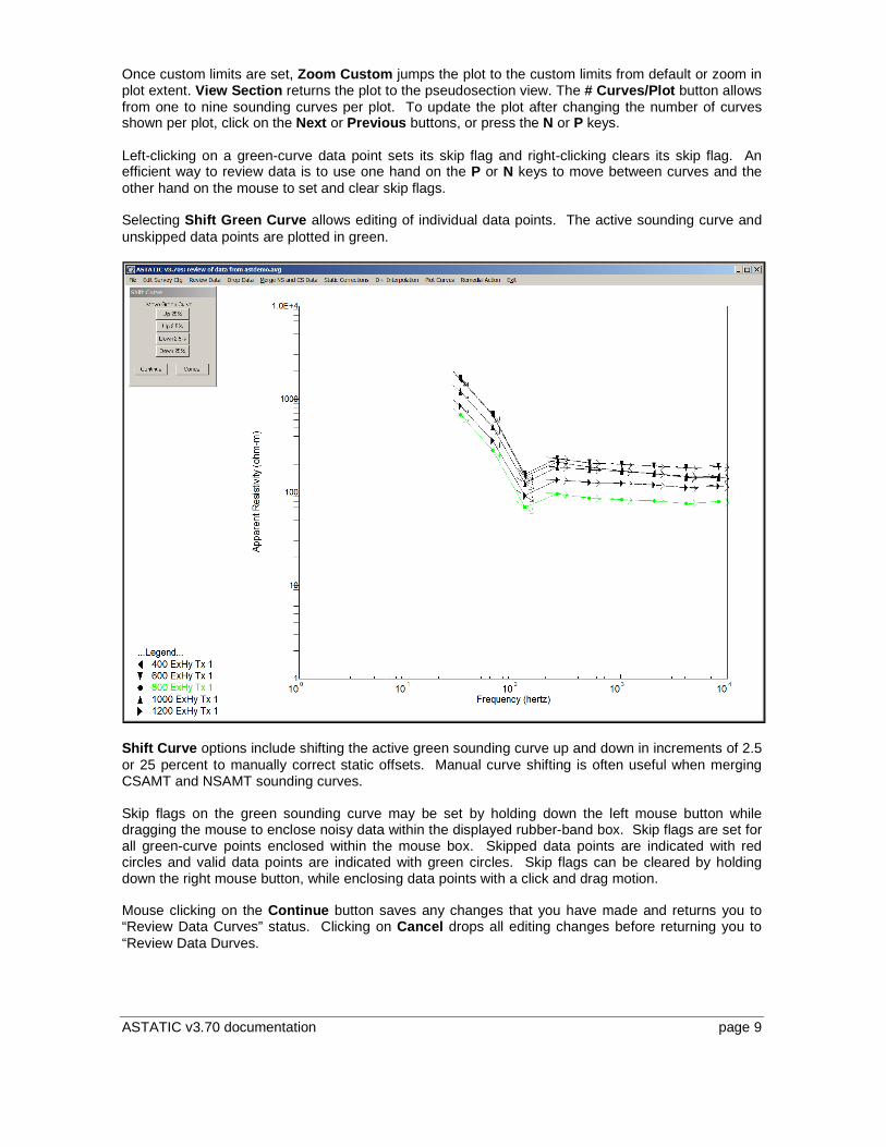
Once custom limits are set, Zoom Custom jumps the plot to the custom limits from default or zoom in plot extent. View Section returns the plot to the pseudosection view. The # Curves/Plot button allows from one to nine sounding curves per plot. To update the plot after changing the number of curves shown per plot, click on the Next or Previous buttons, or press the N or P keys. Left-clicking on a green-curve data point sets its skip flag and right-clicking clears its skip flag. An efficient way to review data is to use one hand on the P or N keys to move between curves and the other hand on the mouse to set and clear skip flags. Selecting Shift Green Curve allows editing of individual data points. The active sounding curve and unskipped data points are plotted in green.

Shift Curve options include shifting the active green sounding curve up and down in increments of 2.5 or 25 percent to manually correct static offsets. Manual curve shifting is often useful when merging CSAMT and NSAMT sounding curves. Skip flags on the green sounding curve may be set by holding down the left mouse button while dragging the mouse to enclose noisy data within the displayed rubber-band box. Skip flags are set for all green-curve points enclosed within the mouse box. Skipped data points are indicated with red circles and valid data points are indicated with green circles. Skip flags can be cleared by holding down the right mouse button, while enclosing data points with a click and drag motion. Mouse clicking on the Continue button saves any changes that you have made and returns you to “Review Data Curves” status. Clicking on Cancel drops all editing changes before returning you to “Review Data Durves.


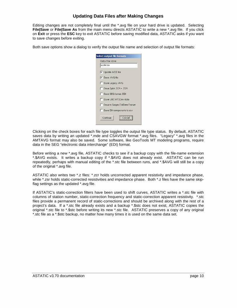
Updating Data Files after Making Changes Editing changes are not completely final until the *.avg file on your hard drive is updated. Selecting File|Save or File|Save As from the main menu directs ASTATIC to write a new *.avg file. If you click on Exit or press the ESC key to exit ASTATIC before saving modified data, ASTATIC asks if you want to save changes before exiting. Both save options show a dialog to verify the output file name and selection of output file formats:

Clicking on the check boxes for each file type toggles the output file type status. By default, ASTATIC saves data by writing an updated *.mde and CSAVGW format *.avg files. “Legacy” *.avg files in the AMTAVG format may also be saved. Some software, like GeoTools MT modeling programs, require data in the SEG “electronic data interchange” (EDI) format. Before writing a new *.avg file, ASTATIC checks to see if a backup copy with the file-name extension *.$AVG exists. It writes a backup copy if *.$AVG does not already exist. ASTATIC can be run repeatedly, perhaps with manual editing of the *.stc file between runs, and *.$AVG will still be a copy of the original *.avg file. ASTATIC also writes two *.z files: *.zcr holds uncorrected apparent resistivity and impedance phase, while *.zsr holds static-corrected resistivities and impedance phase. Both *.z files have the same skip-flag settings as the updated *.avg file. If ASTATIC’s static-correction filters have been used to shift curves, ASTATIC writes a *.stc file with columns of station number, static-correction frequency and static-correction apparent resistivity. *.stc files provide a permanent record of static-corrections and should be archived along with the rest of a project’s data. If a *.stc file already exists and a backup *.$stc does not exist, ASTATIC copies the original *.stc file to *.$stc before writing its new *.stc file. ASTATIC preserves a copy of any original *.stc file as a *.$stc backup, no matter how many times it is used on the same data set.


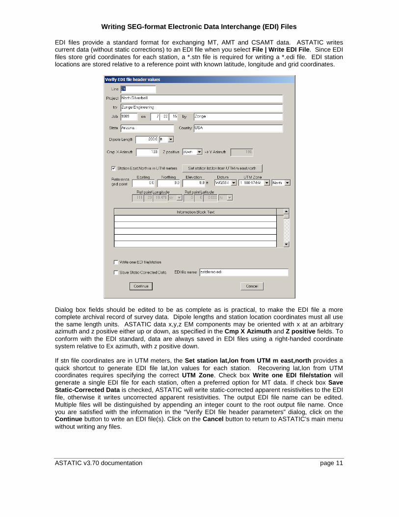
Writing SEG-format Electronic Data Interchange (EDI) Files EDI files provide a standard format for exchanging MT, AMT and CSAMT data. ASTATIC writes current data (without static corrections) to an EDI file when you select File | Write EDI File. Since EDI files store grid coordinates for each station, a *.stn file is required for writing a *.edi file. EDI station locations are stored relative to a reference point with known latitude, longitude and grid coordinates.

Dialog box fields should be edited to be as complete as is practical, to make the EDI file a more complete archival record of survey data. Dipole lengths and station location coordinates must all use the same length units. ASTATIC data x,y,z EM components may be oriented with x at an arbitrary azimuth and z positive either up or down, as specified in the Cmp X Azimuth and Z positive fields. To conform with the EDI standard, data are always saved in EDI files using a right-handed coordinate system relative to Ex azimuth, with z positive down. If stn file coordinates are in UTM meters, the Set station lat,lon from UTM m east,north provides a quick shortcut to generate EDI file lat,lon values for each station. Recovering lat,lon from UTM coordinates requires specifying the correct UTM Zone. Check box Write one EDI file/station will generate a single EDI file for each station, often a preferred option for MT data. If check box Save Static-Corrected Data is checked, ASTATIC will write static-corrected apparent resistivities to the EDI file, otherwise it writes uncorrected apparent resistivities. The output EDI file name can be edited. Multiple files will be distinguished by appending an integer count to the root output file name. Once you are satisfied with the information in the “Verify EDI file header parameters” dialog, click on the Continue button to write an EDI file(s). Click on the Cancel button to return to ASTATIC’s main menu without writing any files.


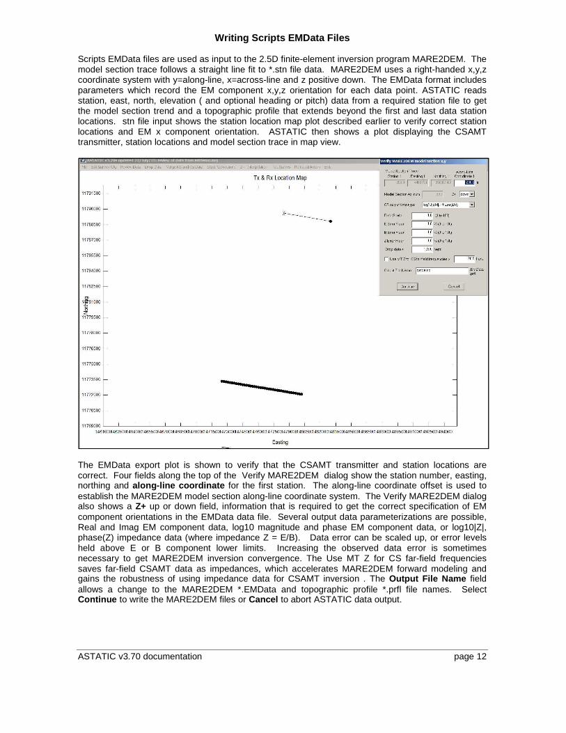
Writing Scripts EMData Files Scripts EMData files are used as input to the 2.5D finite-element inversion program MARE2DEM. The model section trace follows a straight line fit to *.stn file data. MARE2DEM uses a right-handed x,y,z coordinate system with y=along-line, x=across-line and z positive down. The EMData format includes parameters which record the EM component x,y,z orientation for each data point. ASTATIC reads station, east, north, elevation ( and optional heading or pitch) data from a required station file to get the model section trend and a topographic profile that extends beyond the first and last data station locations. stn file input shows the station location map plot described earlier to verify correct station locations and EM x component orientation. ASTATIC then shows a plot displaying the CSAMT transmitter, station locations and model section trace in map view.

The EMData export plot is shown to verify that the CSAMT transmitter and station locations are correct. Four fields along the top of the Verify MARE2DEM dialog show the station number, easting, northing and along-line coordinate for the first station. The along-line coordinate offset is used to establish the MARE2DEM model section along-line coordinate system. The Verify MARE2DEM dialog also shows a Z+ up or down field, information that is required to get the correct specification of EM component orientations in the EMData data file. Several output data parameterizations are possible, Real and Imag EM component data, log10 magnitude and phase EM component data, or log10|Z|, phase(Z) impedance data (where impedance Z = E/B). Data error can be scaled up, or error levels held above E or B component lower limits. Increasing the observed data error is sometimes necessary to get MARE2DEM inversion convergence. The Use MT Z for CS far-field frequencies saves far-field CSAMT data as impedances, which accelerates MARE2DEM forward modeling and gains the robustness of using impedance data for CSAMT inversion . The Output File Name field allows a change to the MARE2DEM *.EMData and topographic profile *.prfl file names. Select Continue to write the MARE2DEM files or Cancel to abort ASTATIC data output.


Drop Data

ASTATIC includes three approaches to windowing data. Auto Skip sets reversible skip flags based on error-level thresholds. Drop skipped data, permanently deletes data points that have skip flags set either by Auto Skip or manually during Data Review quality control editing. Window Data and Drop permanently deletes data based on station number, frequency, frequency, apparent resistivity, impedance phase, Tx ID and impedance type ranges.

Auto Skip

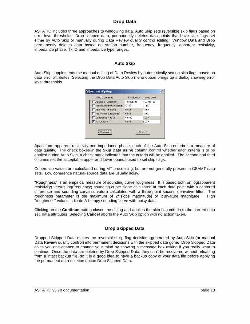
Auto Skip supplements the manual editing of Data Review by automatically setting skip flags based on data error attributes. Selecting the Drop Data|Auto Skip menu option brings up a dialog showing error level thresholds.

Apart from apparent resistivity and impedance phase, each of the Auto Skip criteria is a measure of data quality. The check boxes in the Skip Data using column control whether each criteria is to be applied during Auto Skip, a check mark indicates that the criteria will be applied. The second and third columns set the acceptable upper and lower bounds used to set skip flags. Coherence values are calculated during MT processing, but are not generally present in CSAMT data sets. Low coherence natural-source data are usually noisy. "Roughness" is an empirical measure of sounding curve roughness. It is based both on log(apparent resistivity) versus log(frequency) sounding-curve slope calculated at each data point with a centered difference and sounding curve curvature calculated with a three-point second derivative filter. The roughness parameter is the maximum of 2*|slope magnitude| or |curvature magnitude|. High "roughness" values indicate A bumpy sounding curve with noisy data. Clicking on the Continue button closes the dialog and applies the skip-flag criteria to the current data set. data attributes Selecting Cancel aborts the Auto Skip option with no action taken.

Drop Skipped Data

Dropped Skipped Data makes the reversible skip-flag decisions generated by Auto Skip (or manual Data Review quality control) into permanent decisions with the skipped data gone. Drop Skipped Data gives you one chance to change your mind by showing a message box asking if you really want to continue. Once the data are deleted by Drop Skipped Data, they can't be recovered without reloading from a intact backup file, so it is a good idea to have a backup copy of your data file before applying the permanent data-deletion option Drop Skipped Data.


Window Data and Drop

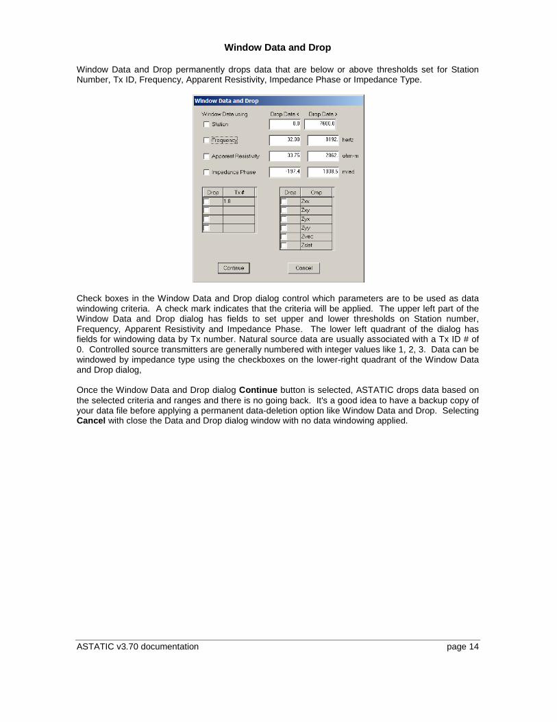
Window Data and Drop permanently drops data that are below or above thresholds set for Station Number, Tx ID, Frequency, Apparent Resistivity, Impedance Phase or Impedance Type.

Check boxes in the Window Data and Drop dialog control which parameters are to be used as data windowing criteria. A check mark indicates that the criteria will be applied. The upper left part of the Window Data and Drop dialog has fields to set upper and lower thresholds on Station number, Frequency, Apparent Resistivity and Impedance Phase. The lower left quadrant of the dialog has fields for windowing data by Tx number. Natural source data are usually associated with a Tx ID # of 0. Controlled source transmitters are generally numbered with integer values like 1, 2, 3. Data can be windowed by impedance type using the checkboxes on the lower-right quadrant of the Window Data and Drop dialog, Once the Window Data and Drop dialog Continue button is selected, ASTATIC drops data based on the selected criteria and ranges and there is no going back. It's a good idea to have a backup copy of your data file before applying a permanent data-deletion option like Window Data and Drop. Selecting Cancel with close the Data and Drop dialog window with no data windowing applied.


Merge NS and CS data

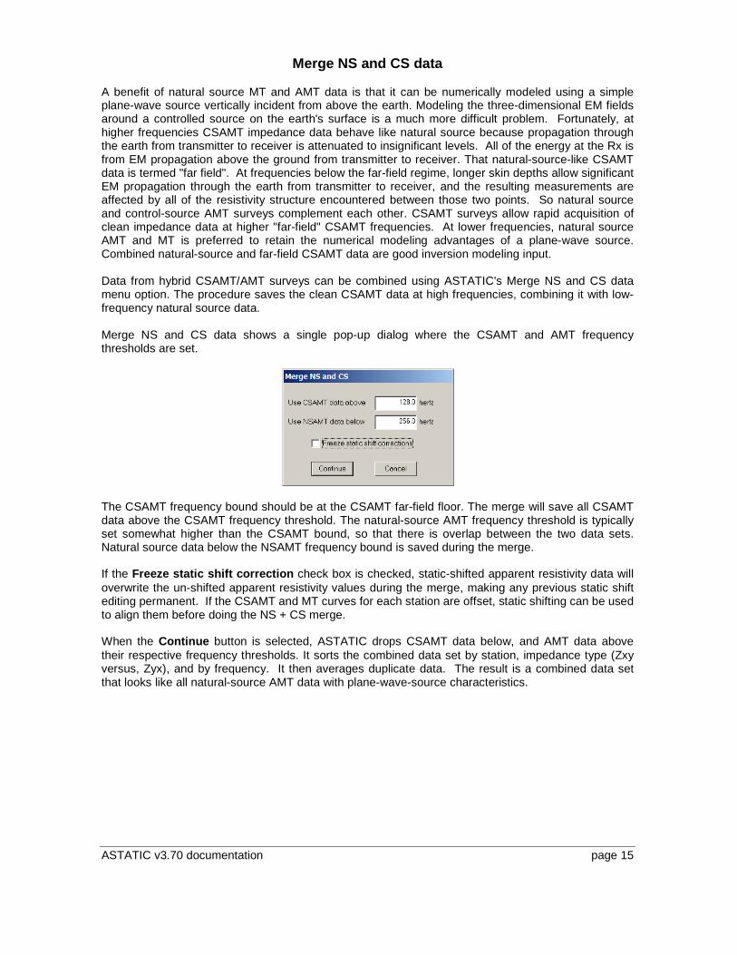
A benefit of natural source MT and AMT data is that it can be numerically modeled using a simple plane-wave source vertically incident from above the earth. Modeling the three-dimensional EM fields around a controlled source on the earth's surface is a much more difficult problem. Fortunately, at higher frequencies CSAMT impedance data behave like natural source because propagation through the earth from transmitter to receiver is attenuated to insignificant levels. All of the energy at the Rx is from EM propagation above the ground from transmitter to receiver. That natural-source-like CSAMT data is termed "far field". At frequencies below the far-field regime, longer skin depths allow significant EM propagation through the earth from transmitter to receiver, and the resulting measurements are affected by all of the resistivity structure encountered between those two points. So natural source and control-source AMT surveys complement each other. CSAMT surveys allow rapid acquisition of clean impedance data at higher "far-field" CSAMT frequencies. At lower frequencies, natural source AMT and MT is preferred to retain the numerical modeling advantages of a plane-wave source. Combined natural-source and far-field CSAMT data are good inversion modeling input. Data from hybrid CSAMT/AMT surveys can be combined using ASTATIC's Merge NS and CS data menu option. The procedure saves the clean CSAMT data at high frequencies, combining it with low-frequency natural source data. Merge NS and CS data shows a single pop-up dialog where the CSAMT and AMT frequency thresholds are set.

The CSAMT frequency bound should be at the CSAMT far-field floor. The merge will save all CSAMT data above the CSAMT frequency threshold. The natural-source AMT frequency threshold is typically set somewhat higher than the CSAMT bound, so that there is overlap between the two data sets. Natural source data below the NSAMT frequency bound is saved during the merge. If the Freeze static shift correction check box is checked, static-shifted apparent resistivity data will overwrite the un-shifted apparent resistivity values during the merge, making any previous static shift editing permanent. If the CSAMT and MT curves for each station are offset, static shifting can be used to align them before doing the NS + CS merge. When the Continue button is selected, ASTATIC drops CSAMT data below, and AMT data above their respective frequency thresholds. It sorts the combined data set by station, impedance type (Zxy versus, Zyx), and by frequency. It then averages duplicate data. The result is a combined data set that looks like all natural-source AMT data with plane-wave-source characteristics.


Static Corrections

Static corrections are most useful for conditioning data before inversion with one-dimensional modeling programs, like CSINV and SCSINV. Two-dimension inversion programs, like SCS2D, can model static offsets directly by introducing near-surface structure into the inversion model section. Static-correction procedures attempt to minimize the effects of localized changes in near-surface resistivity by shifting CSAMT sounding curves of log(apparent resistivity versus log(frequency), without changing their shape. Multiplying all apparent resistivities in a particular sounding curve by the same correction factor has the effect of shifting the sounding curve without changing its shape in a log(resistivity) versus log(frequency) presentation. Estimating average near-surface resistivity is central to calculating static-correction offsets. ASTATIC includes four methods for calculating near-surface resistivities. Method 1 is to use independent measurements of near-surface resistivity, such as TEM soundings, to shift the CSAMT sounding curves to match the TEM results. If independent near-surface resistivity information is not available, methods 2, 3 or 4 can be used. In method 2, ASTATIC uses a trimmed-moving-average (TMA) filter to estimate average resistivities along line at a selected frequency, then shifts sounding curves to match the average resistivities. The TMA filter is designed to remove single-station offsets while preserving broader scale changes. Five-point TMA filtering is Zonge’s most often used static-correction method. In method 3, ASTATIC uses a fixed-length-moving-average (FLMA) filter along line at a selected frequency to estimate static-corrected resistivity shifts. FLMA filtering is most useful for consistent treatment of data sets with different station spacing or dipole lengths. Method 4 is to use an adaptive-moving-average (AMA) filter. An AMA filter length is specified in skin depths and changes based on the average apparent resistivity at the static-correction frequency in the neighborhood of each station. Method 1: Independent: Use independent near-surface resistivity estimates from *.stc files or by rerunning ASTATIC after editing target apparent resistivities in *.stc file at selected stations. Independent near-surface resistivity estimates are often derived from TEM soundings. TEM window times can be converted to frequency using the approximation: frequency = 194/time, with frequency in hertz and time in msec. If a *.stc file is available with the same filename stem as the input *.avg file, method 1 can be used. ASTATIC expects three columns of values in *.stc files: station number, static-correction reference frequency (hertz), and target apparent resistivity (ohm-m). Comment lines are flagged by a "\" or a "!" in the first column. Once the *.stc data are read into ASTATIC, the program shifts each CSAMT apparent resistivity sounding curve by a constant multiplier to match the target apparent resistivity at the static-correction frequency. The reference frequency does not have to match a CSAMT sounding curve frequency. If necessary, ASTATIC will interpolate between CSAMT frequencies. Method 2: TMA: Use a trimmed-moving-average filter to estimate average apparent resistivities at a single static-correction-reference frequency. The TMA filter option estimates near-surface resistivities by averaging apparent resistivities along line at the selected static-correction reference frequency. The highest frequency with clean data should be selected as the reference frequency. 1) Sounding curves are first interpolated to the reference frequency to get an array of uncorrected apparent resistivities, r

j (ohm-m) and impedance phase, ϕ

j (mrad), for each station, j = 1 to n.

2) Calculate the slope of log(r

j) versus log(frequency) for each station at the normalization frequency:


2

4atan

jslopeπ

π

φ

−

=

11000j

where φj is divided by 1000 to convert mrad to radians. 3) Use slope to extrapolate up in frequency by a factor of sqrt(2).

( ) ( ) ( )log log logρ ρj j jslope+ = + ⋅2

4) For each station collect a group of five log(rj

+), i.e. for station index j, i = j-2 to j+2.

5) Discard the lowest and highest valued log(rj

+) from the group of five and average the remaining

three => avg_logj.

6) The target static-correction apparent resistivity for station j is

( )ρ ρ

ρstatic j j

j

j

avg= ⋅ +

exp _ log for j = 1 to n.

7) Shift sounding curves at all frequencies by multiplying by factor rstatic

j/r

j.

Method 3: FLMA: Use a fixed-length-moving-average filter to estimate average apparent resistivities at a single static-correction-reference frequency. The FLMA filter estimates static-corrected apparent resistivities at a single reference frequency by calculating a profile of average impedances along the length of the line. Sounding curves are then shifted so that they intersect the averaged profile. The highest frequency with clean data should be selected as the static-correction reference frequency. 1) Sounding curves are first interpolated to the reference frequency to get an array of uncorrected apparent resistivities, r



Apparent resistivity and impedance phase are converted to impedance values, Zj, for each station.

( ) ( ) ( )( )Z ij j= ⋅ ⋅ ⋅ + ⋅

⋅ ⋅ ⋅ ⋅

ρ ω µ φ φ

ρ

φ

ω π µ π

cos

where

is uncorrected apparent resistivity (ohm - m) at f,

is impedance phase (mrad) at f,

f is static - correction reference frequency (hertz),

= 2 f, = 4 10 and i = -1

j j

j

j

-7

1000 1000sin

. 2) Impedances are averaged with a fixed-length Hanning window centered on each station in turn. The filter width is set to five dipole lengths by default, but can be changed to any value between 1 and 100 dipole lengths. Filter weights are adjusted for finite-length dipoles by integrating a segment of the Hanning window over one dipole length at each station.


( )Zavg w Zj k kk

n

= ⋅

==∑

1

0where wk outside of the Hanning window and w is integrated over one dipole length

within the Hanning window.

k

3) Recover static-corrected apparent resistivity at reference frequency from Z

j.

ρ

ω µstatic j =

⋅

Z j2


j/r

j.

Method 4: AMA: Use an adaptive-moving-average filter to estimate average apparent resistivities at a single static-correction-reference frequency. Adaptive filtering is based on ideas presented in Torres-Verdin and Bostick, 1992, Principles of spatial surface electric field filtering in magnetotellurics: electromagnetic array profiling (EMAP), Geophysics, v57, p603-622. The AMA filter estimates static-corrected apparent resistivities at a single reference frequency by calculating a profile of average impedances along the length of the line. Sounding curves are then shifted so that they intersect the averaged profile. The highest frequency with clean data should be selected as the static-correction reference frequency. 1) Sounding curves are first interpolated to the reference frequency to get an array of uncorrected apparent resistivities, r



Apparent resistivity and impedance phase are converted to impedance values, Zj, for each station.

( ) ( ) ( )( )Z ij j= ⋅ ⋅ ⋅ + ⋅

⋅ ⋅ ⋅ ⋅

ρ ω µ φ φ

ρ

φ

ω π µ π

cos

where

is uncorrected apparent resistivity (ohm - m) at f,

is impedance phase (mrad) at f,

f is static - correction reference frequency (hertz),

= 2 f, = 4 10 and i = -1

j j

j

j

-7

1000 1000sin

. 2) Impedances are averaged with a variable-length Hanning window centered on each station in turn. Filter lengths are adjusted iteratively at each station, using the average apparent resistivity to calculate a filter width, then using the filter to calculate a new average apparent resistivity. The filter width is set to one skin depth, but can be changed to any value between 1 and 10 skin depths. Individual filter weights are adjusted for finite-length dipoles by integrating over a one-dipole-length segment of the Hanning window at each station.

( )Zavg w Zj k kk

n

= ⋅

==∑

1

0where wk outside of the Hanning window and w is integrated over one dipole length

within the Hanning window.

k


3) Recover static-corrected apparent resistivity at reference frequency from Z

j.

ρ

ω µstatic j =

⋅

Z j2


j/r

j.

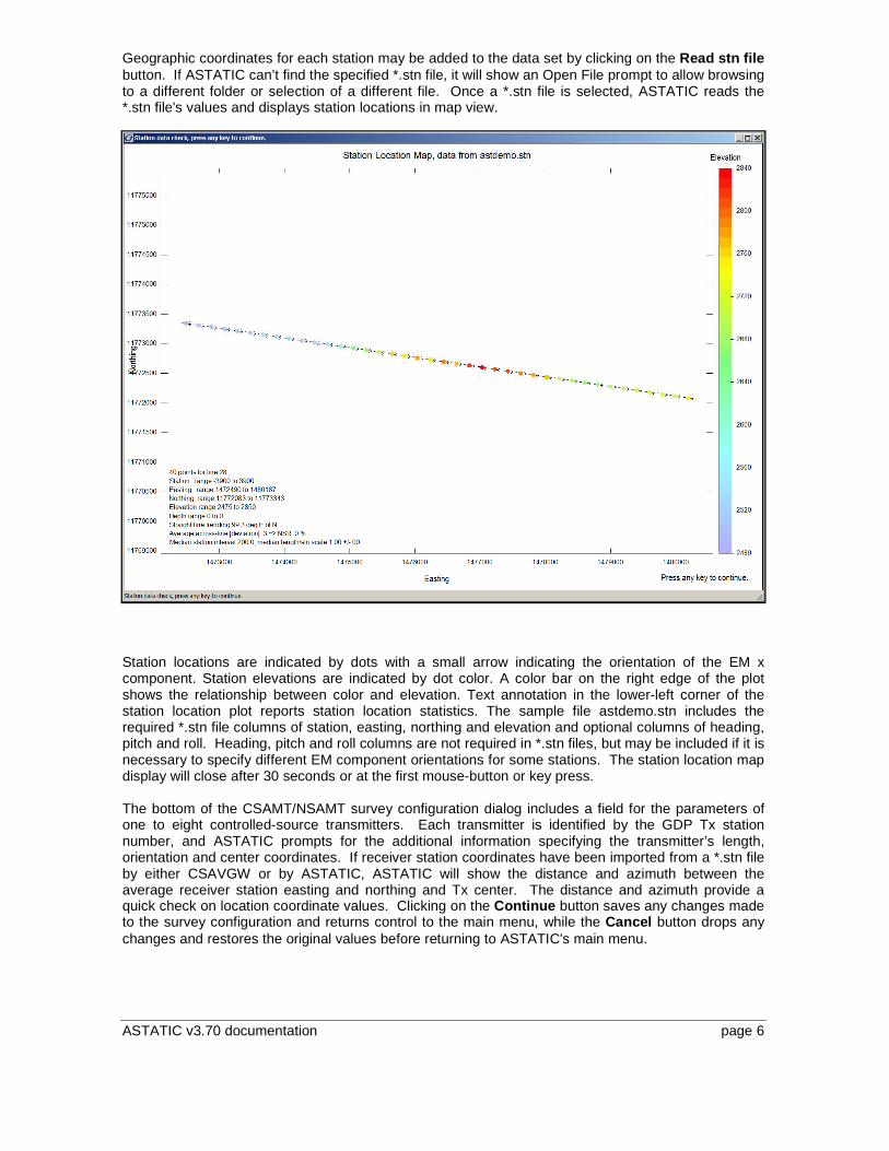
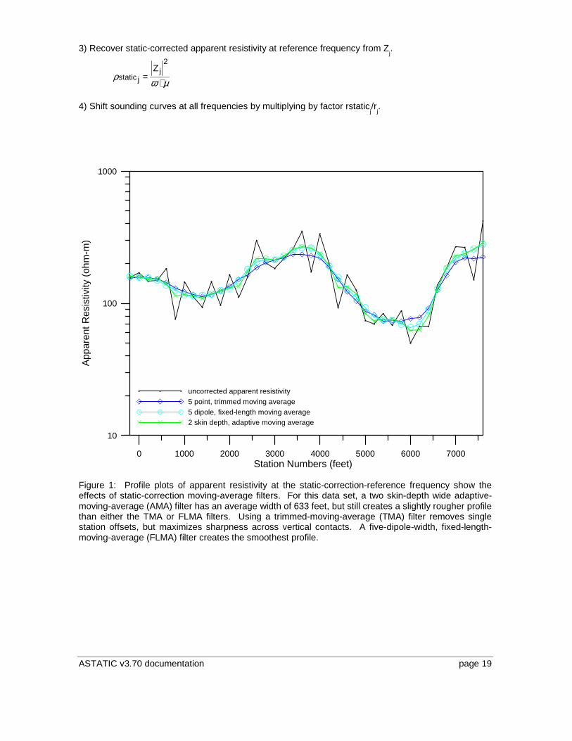
Figure 1: Profile plots of apparent resistivity at the static-correction-reference frequency show the effects of static-correction moving-average filters. For this data set, a two skin-depth wide adaptive-moving-average (AMA) filter has an average width of 633 feet, but still creates a slightly rougher profile than either the TMA or FLMA filters. Using a trimmed-moving-average (TMA) filter removes single station offsets, but maximizes sharpness across vertical contacts. A five-dipole-width, fixed-length-moving-average (FLMA) filter creates the smoothest profile.

0 1000 2000 3000 4000 5000 6000 7000Station Numbers (feet)

10

100

1000

App

aren

t Res

istiv

ity (

ohm

-m)

uncorrected apparent resistivity5 point, trimmed moving average5 dipole, fixed-length moving average2 skin depth, adaptive moving average


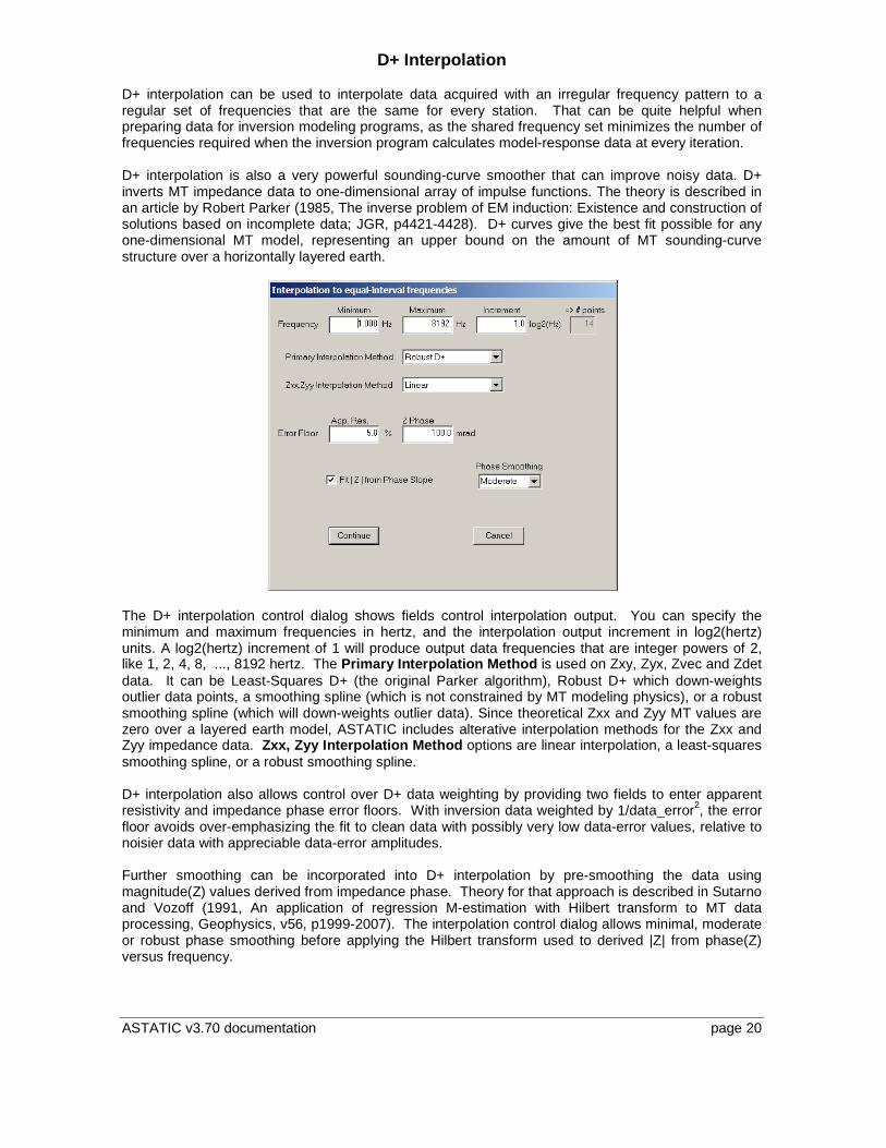
D+ Interpolation D+ interpolation can be used to interpolate data acquired with an irregular frequency pattern to a regular set of frequencies that are the same for every station. That can be quite helpful when preparing data for inversion modeling programs, as the shared frequency set minimizes the number of frequencies required when the inversion program calculates model-response data at every iteration. D+ interpolation is also a very powerful sounding-curve smoother that can improve noisy data. D+ inverts MT impedance data to one-dimensional array of impulse functions. The theory is described in an article by Robert Parker (1985, The inverse problem of EM induction: Existence and construction of solutions based on incomplete data; JGR, p4421-4428). D+ curves give the best fit possible for any one-dimensional MT model, representing an upper bound on the amount of MT sounding-curve structure over a horizontally layered earth.

The D+ interpolation control dialog shows fields control interpolation output. You can specify the minimum and maximum frequencies in hertz, and the interpolation output increment in log2(hertz) units. A log2(hertz) increment of 1 will produce output data frequencies that are integer powers of 2, like 1, 2, 4, 8, ..., 8192 hertz. The Primary Interpolation Method is used on Zxy, Zyx, Zvec and Zdet data. It can be Least-Squares D+ (the original Parker algorithm), Robust D+ which down-weights outlier data points, a smoothing spline (which is not constrained by MT modeling physics), or a robust smoothing spline (which will down-weights outlier data). Since theoretical Zxx and Zyy MT values are zero over a layered earth model, ASTATIC includes alterative interpolation methods for the Zxx and Zyy impedance data. Zxx, Zyy Interpolation Method options are linear interpolation, a least-squares smoothing spline, or a robust smoothing spline. D+ interpolation also allows control over D+ data weighting by providing two fields to enter apparent resistivity and impedance phase error floors. With inversion data weighted by 1/data_error2, the error floor avoids over-emphasizing the fit to clean data with possibly very low data-error values, relative to noisier data with appreciable data-error amplitudes. Further smoothing can be incorporated into D+ interpolation by pre-smoothing the data using magnitude(Z) values derived from impedance phase. Theory for that approach is described in Sutarno and Vozoff (1991, An application of regression M-estimation with Hilbert transform to MT data processing, Geophysics, v56, p1999-2007). The interpolation control dialog allows minimal, moderate or robust phase smoothing before applying the Hilbert transform used to derived |Z| from phase(Z) versus frequency.


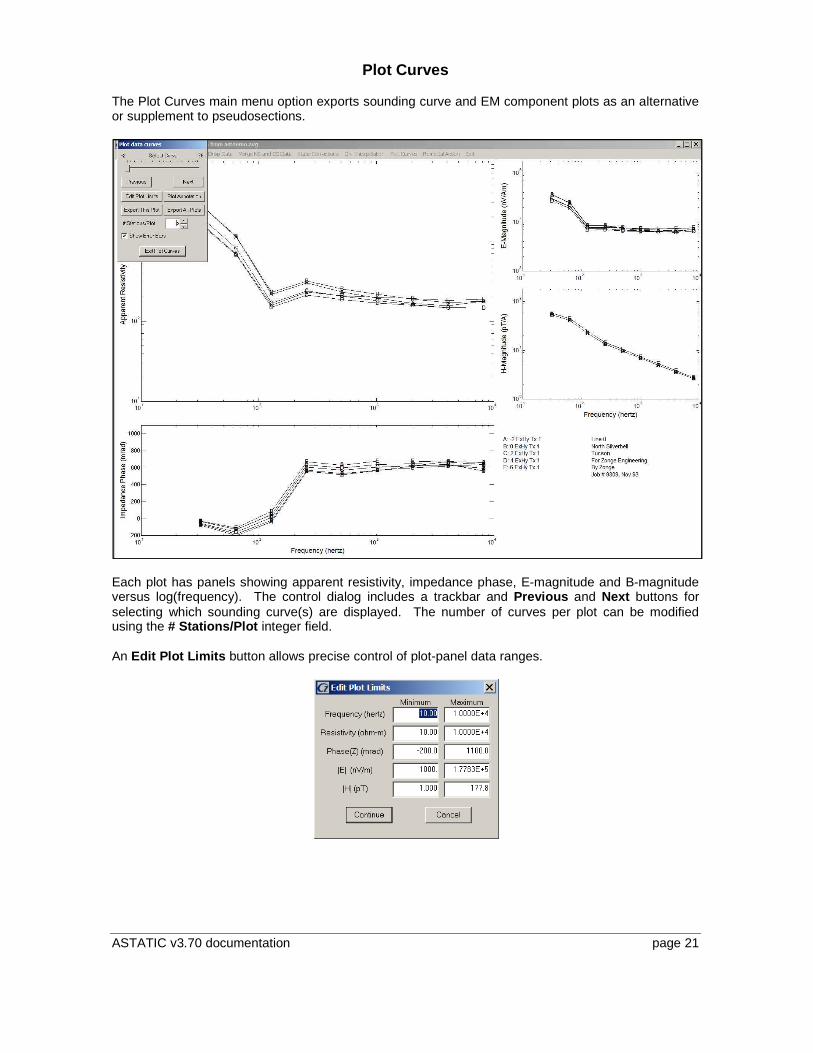
Plot Curves

The Plot Curves main menu option exports sounding curve and EM component plots as an alternative or supplement to pseudosections.

Each plot has panels showing apparent resistivity, impedance phase, E-magnitude and B-magnitude versus log(frequency). The control dialog includes a trackbar and Previous and Next buttons for selecting which sounding curve(s) are displayed. The number of curves per plot can be modified using the # Stations/Plot integer field. An Edit Plot Limits button allows precise control of plot-panel data ranges.


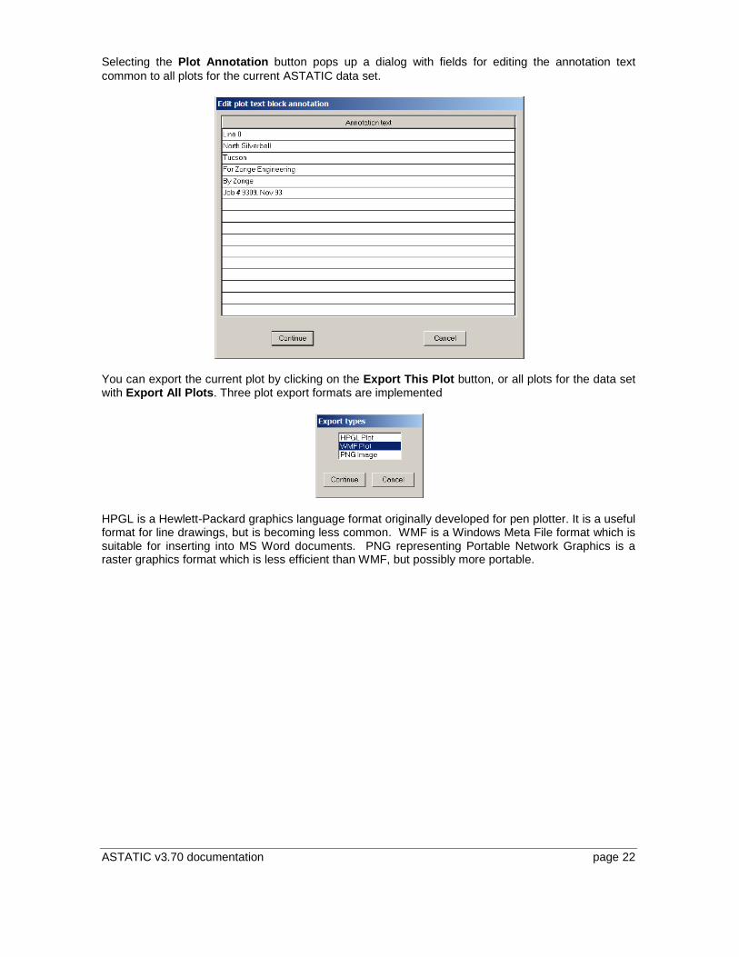
Selecting the Plot Annotation button pops up a dialog with fields for editing the annotation text common to all plots for the current ASTATIC data set.

You can export the current plot by clicking on the Export This Plot button, or all plots for the data set with Export All Plots. Three plot export formats are implemented

HPGL is a Hewlett-Packard graphics language format originally developed for pen plotter. It is a useful format for line drawings, but is becoming less common. WMF is a Windows Meta File format which is suitable for inserting into MS Word documents. PNG representing Portable Network Graphics is a raster graphics format which is less efficient than WMF, but possibly more portable.


Remedial Action

|Z| from smoothed phase(Z)

Due to the causal nature of MT data, the way impedance amplitude changes as a function of frequency is related to impedance phase by a Hilbert transform (Sutarno and Vozoff, 1991, An application of regression M-estimation with Hilbert transform to MT data processing, Geophysics, v56, p1999-2007). Many times the impedance phase values are cleaner than the impedance magnitude (and apparent resistivity based on impedance magnitude). Each station's impedance phase curve is fit with a smoothing spline, so that values can be recovered at the frequencies needed for a Hilbert transform. The Hilbert transform yields a impedance magnitude or derived apparent resistivity) curve which is generally smoother than the original measurements. |Z| from phase values are recovered for the original measured frequency set.

Robust 2D Smoothing Filter

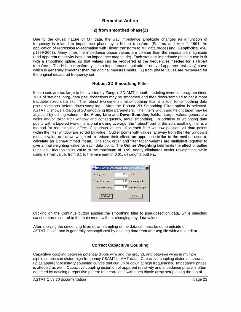
If data sets are too large to be inverted by Zonge’s 2D AMT smooth-modeling inversion program (lines 100s of stations long), data pseudosections may be smoothed and then down-sampled to get a more tractable sized data set. The robust two-dimensional smoothing filter is a tool for smoothing data pseudosections before down-sampling. After the Robust 2D Smoothing Filter option is selected, ASTATIC shows a dialog of 2D smoothing filter parameters. The filter’s width and height taper may be adjusted by editing values in the Along Line and Down Sounding fields. Larger values generate a wider and/or taller filter window and consequently, more smoothing. In addition to weighting data points with a tapered two-dimensional moving average, the “robust” part of the 2d smoothing filter is a method for reducing the effect of spurious values. For each filter window position, all data points within the filter window are sorted by value. Outlier points with values far away from the filter window’s median value are down-weighted to reduce their effect, an approach similar to the method used to calculate an alpha-trimmed mean. The rank order and filter taper weights are multiplied together to give a final weighting value for each data point. The Outlier Weighting field limits the effect of outlier rejection. Increasing its value to the maximum of 0.99, nearly eliminates outlier reweighting, while using a small value, from 0.1 to the minimum of 0.01, deweights outliers.

Clicking on the Continue button applies the smoothing filter to pseudosection data, while selecting cancel returns control to the main menu without changing any data values. After applying the smoothing filter, down-sampling of the data set must be done outside of ASTATIC.exe, and is generally accomplished by deleting data from an *.avg file with a text editor.

Correct Capacitive Coupling Capacitive coupling between potential dipole wire and the ground, and between wires in multiple dipole setups can distort high frequency CSAMT or AMT data. Capacitive coupling distortion shows up as apparent resistivity sounding curves that curl up or down at high frequencies. Impedance phase is affected as well. Capacitive coupling distortion of apparent resistivity and impedance phase is often detected by noticing a repetitive pattern that correlates with each dipole array setup along the top of


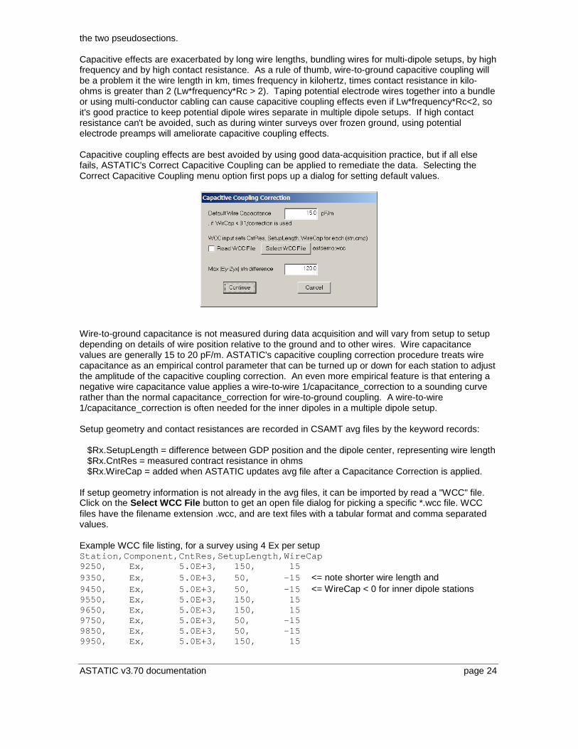
the two pseudosections. Capacitive effects are exacerbated by long wire lengths, bundling wires for multi-dipole setups, by high frequency and by high contact resistance. As a rule of thumb, wire-to-ground capacitive coupling will be a problem it the wire length in km, times frequency in kilohertz, times contact resistance in kilo-ohms is greater than 2 (Lw*frequency*Rc > 2). Taping potential electrode wires together into a bundle or using multi-conductor cabling can cause capacitive coupling effects even if Lw*frequency*Rc<2, so it's good practice to keep potential dipole wires separate in multiple dipole setups. If high contact resistance can't be avoided, such as during winter surveys over frozen ground, using potential electrode preamps will ameliorate capacitive coupling effects. Capacitive coupling effects are best avoided by using good data-acquisition practice, but if all else fails, ASTATIC's Correct Capacitive Coupling can be applied to remediate the data. Selecting the Correct Capacitive Coupling menu option first pops up a dialog for setting default values.

Wire-to-ground capacitance is not measured during data acquisition and will vary from setup to setup depending on details of wire position relative to the ground and to other wires. Wire capacitance values are generally 15 to 20 pF/m. ASTATIC's capacitive coupling correction procedure treats wire capacitance as an empirical control parameter that can be turned up or down for each station to adjust the amplitude of the capacitive coupling correction. An even more empirical feature is that entering a negative wire capacitance value applies a wire-to-wire 1/capacitance_correction to a sounding curve rather than the normal capacitance_correction for wire-to-ground coupling. A wire-to-wire 1/capacitance_correction is often needed for the inner dipoles in a multiple dipole setup. Setup geometry and contact resistances are recorded in CSAMT avg files by the keyword records: $Rx.SetupLength = difference between GDP position and the dipole center, representing wire length $Rx.CntRes = measured contract resistance in ohms $Rx.WireCap = added when ASTATIC updates avg file after a Capacitance Correction is applied. If setup geometry information is not already in the avg files, it can be imported by read a "WCC" file. Click on the Select WCC File button to get an open file dialog for picking a specific *.wcc file. WCC files have the filename extension .wcc, and are text files with a tabular format and comma separated values. Example WCC file listing, for a survey using 4 Ex per setup Station,Component,CntRes,SetupLength,WireCap 9250, Ex, 5.0E+3, 150, 15 9350, Ex, 5.0E+3, 50, -15 <= note shorter wire length and 9450, Ex, 5.0E+3, 50, -15 <= WireCap < 0 for inner dipole stations 9550, Ex, 5.0E+3, 150, 15 9650, Ex, 5.0E+3, 150, 15 9750, Ex, 5.0E+3, 50, -15 9850, Ex, 5.0E+3, 50, -15 9950, Ex, 5.0E+3, 150, 15


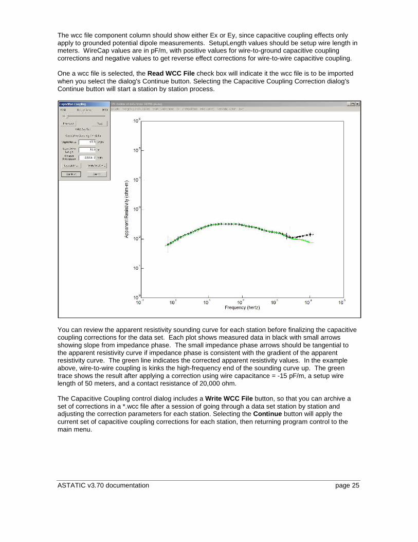
The wcc file component column should show either Ex or Ey, since capacitive coupling effects only apply to grounded potential dipole measurements. SetupLength values should be setup wire length in meters. WireCap values are in pF/m, with positive values for wire-to-ground capacitive coupling corrections and negative values to get reverse effect corrections for wire-to-wire capacitive coupling. One a wcc file is selected, the Read WCC File check box will indicate it the wcc file is to be imported when you select the dialog's Continue button. Selecting the Capacitive Coupling Correction dialog's Continue button will start a station by station process.

You can review the apparent resistivity sounding curve for each station before finalizing the capacitive coupling corrections for the data set. Each plot shows measured data in black with small arrows showing slope from impedance phase. The small impedance phase arrows should be tangential to the apparent resistivity curve if impedance phase is consistent with the gradient of the apparent resistivity curve. The green line indicates the corrected apparent resistivity values. In the example above, wire-to-wire coupling is kinks the high-frequency end of the sounding curve up. The green trace shows the result after applying a correction using wire capacitance = -15 pF/m, a setup wire length of 50 meters, and a contact resistance of 20,000 ohm. The Capacitive Coupling control dialog includes a Write WCC File button, so that you can archive a set of corrections in a *.wcc file after a session of going through a data set station by station and adjusting the correction parameters for each station. Selecting the Continue button will apply the current set of capacitive coupling corrections for each station, then returning program control to the main menu.


Rescale station numbers

Occasionally, it is necessary to rescale station numbers with an offset and linear multiplier. The Rescale station numbers option applies that change.

The rescaling of both the original GDP and Client station numbers is controlled by entering a new station number start value and a station number increment. A negative increment will reverse the direction in which station numbers increase along line.

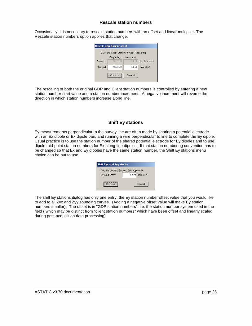
Shift Ey stations Ey measurements perpendicular to the survey line are often made by sharing a potential electrode with an Ex dipole or Ex dipole pair, and running a wire perpendicular to line to complete the Ey dipole. Usual practice is to use the station number of the shared potential electrode for Ey dipoles and to use dipole mid-point station numbers for Ex along-line dipoles. If that station numbering convention has to be changed so that Ex and Ey dipoles have the same station number, the Shift Ey stations menu choice can be put to use.

The shift Ey stations dialog has only one entry, the Ey station number offset value that you would like to add to all Zyx and Zyy sounding curves. (Adding a negative offset value will make Ey station numbers smaller). The offset is in "GDP station numbers", i.e. the station number system used in the field ( which may be distinct from "client station numbers" which have been offset and linearly scaled during post-acquisition data processing).


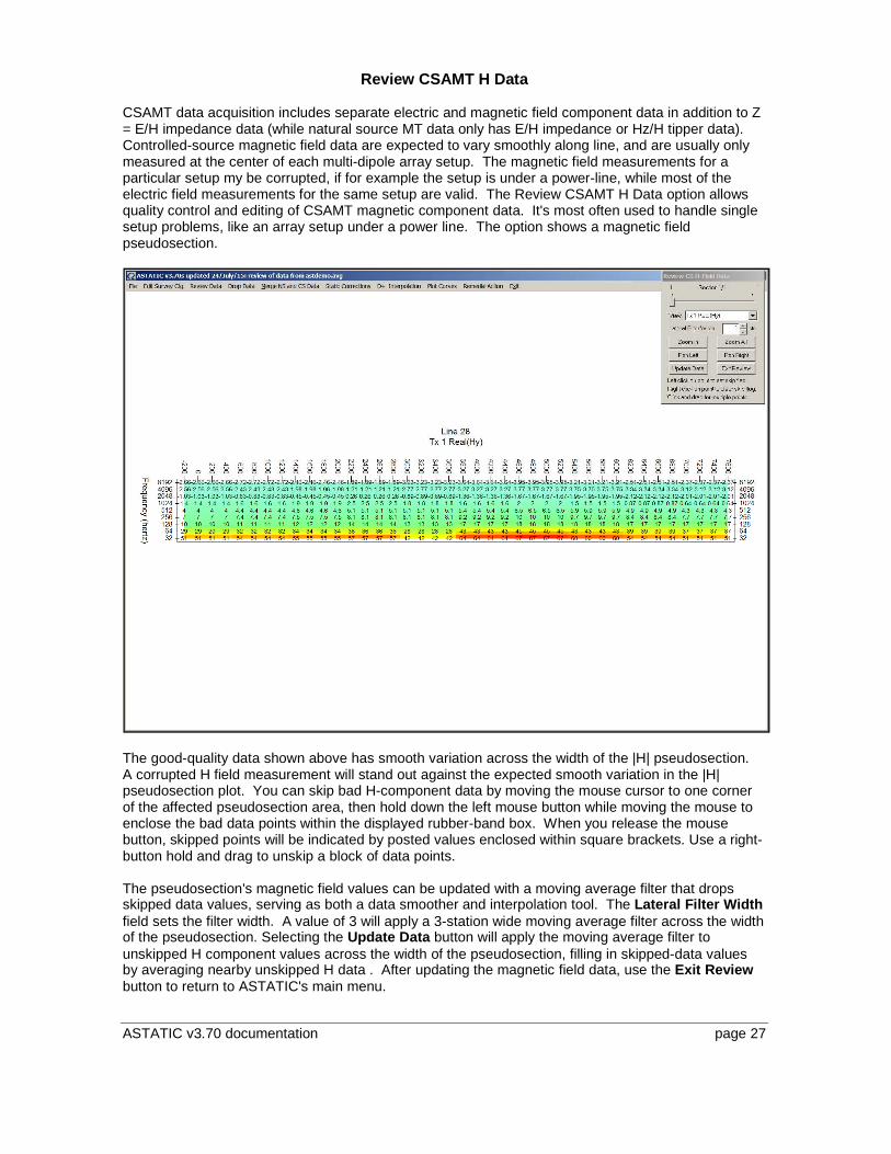
Review CSAMT H Data

CSAMT data acquisition includes separate electric and magnetic field component data in addition to Z = E/H impedance data (while natural source MT data only has E/H impedance or Hz/H tipper data). Controlled-source magnetic field data are expected to vary smoothly along line, and are usually only measured at the center of each multi-dipole array setup. The magnetic field measurements for a particular setup my be corrupted, if for example the setup is under a power-line, while most of the electric field measurements for the same setup are valid. The Review CSAMT H Data option allows quality control and editing of CSAMT magnetic component data. It's most often used to handle single setup problems, like an array setup under a power line. The option shows a magnetic field pseudosection.

The good-quality data shown above has smooth variation across the width of the |H| pseudosection. A corrupted H field measurement will stand out against the expected smooth variation in the |H| pseudosection plot. You can skip bad H-component data by moving the mouse cursor to one corner of the affected pseudosection area, then hold down the left mouse button while moving the mouse to enclose the bad data points within the displayed rubber-band box. When you release the mouse button, skipped points will be indicated by posted values enclosed within square brackets. Use a right-button hold and drag to unskip a block of data points. The pseudosection's magnetic field values can be updated with a moving average filter that drops skipped data values, serving as both a data smoother and interpolation tool. The Lateral Filter Width field sets the filter width. A value of 3 will apply a 3-station wide moving average filter across the width of the pseudosection. Selecting the Update Data button will apply the moving average filter to unskipped H component values across the width of the pseudosection, filling in skipped-data values by averaging nearby unskipped H data . After updating the magnetic field data, use the Exit Review button to return to ASTATIC's main menu.



Installation Notes ASTATIC requires a computer running Microsoft Windows. The following files should be distributed with ASTATIC: astatic.exe 32-bit executable program astatic64.exe 64-bit executable program astdemo.avg sample CSAVGW -format *.avg file astdemo.$avg original sample AMTAVG format *.avg file astdemo0.avg sample legacy AMTAVG-format *.avg file astdemo.mde holds station number scaling and shifting parameters astdemo.stn sample *.stn file with column labels and EM component azimuth columns astdemo.zcr ZPlot *.z file with uncorrected data from astdemo.avg astdemo.zsr ZPlot *.z file with static-corrected data from astdemo.avg astdemo.stc static-correction frequencies and target apparent resistivities Astatic.exe may be put anywhere on the MS-DOS path for use from the MS-DOS command line. It may also be run from the start menu or from a Windows shortcut.

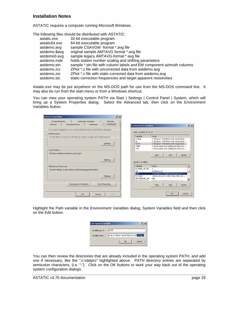
You can view your operating system PATH via Start | Settings | Control Panel | System, which will bring up a System Properties dialog. Select the Advanced tab, then click on the Environment Variables button.

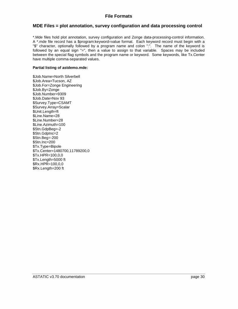
Highlight the Path variable in the Environment Variables dialog, System Variables field and then click on the Edit button.

You can then review the directories that are already included in the operating system PATH, and add one if necessary, like the “;c:\datpro” highlighted above. PATH directory entries are separated by semicolon characters, (i.e. “;”). Click on the OK buttons to work your way back out of the operating system configuration dialogs.


File Formats MDE Files = plot annotation, survey configuration and data processing control

*.Mde files hold plot annotation, survey configuration and Zonge data-processing-control information. A *.mde file record has a $program:keyword=value format. Each keyword record must begin with a "$" character, optionally followed by a program name and colon ":". The name of the keyword is followed by an equal sign "=", then a value to assign to that variable. Spaces may be included between the special flag symbols and the program name or keyword. Some keywords, like Tx.Center have multiple comma-separated values. Partial listing of astdemo.mde: $Job.Name=North Silverbell $Job.Area=Tucson, AZ $Job.For=Zonge Engineering $Job.By=Zonge $Job.Number=9309 $Job.Date=Nov 93 $Survey.Type=CSAMT $Survey.Array=Scalar $Unit.Length=ft $Line.Name=28 $Line.Number=28 $Line.Azimuth=100 $Stn.GdpBeg=-2 $Stn.GdpInc=2 $Stn.Beg=-200 $Stn.Inc=200 $Tx.Type=Bipole $Tx.Center=1480700,11789200,0 $Tx.HPR=100,0,0 $Tx.Length=5000 ft $Rx.HPR=100,0,0 $Rx.Length=200 ft


ASTATIC *.mde keyword descriptions: Survey annotation $Job.Name project name (128 character string) (alias = Project) $Job.Area project area (128 character string) $Job.For client or customer name (128 character string) (alias = client) $Job.By contractor or data acquisition company (128 character string) (alias = company) $Job.Number job label (16 character string) (alias = JobNumb) $Job.Date data acquisition data (16 character string) (alias =JobDate) Survey configuration $Survey.Type survey type (CSAMT, TEM, CR, TDIP) $Survey.Array array type (for CSAMT: Scalar, Vector, Tensor) $Unit.Length length unit (m,ft) (alias = Units) $Line.Name line label (16 character string) (alias = JobLine) $Line.Number line number (float) $Line.Azimuth line azimuth (float, deg E of N) (alias = BrgLine) $Stn.GdpBeg first gdp station number (float) (alias = StnBeg) $Stn.GdpInc gdp station number increment (non-zero float) (alias = StnDelt) $Stn.Beg possibly rescaled first station number (float) (alias = LblFrst) $Stn.Inc possibly rescaled station number increment (float) (alias = LblDelt) $Tx.Type source type (for NSAMT /CSAMT: Natural, Bipole, Loop) $Tx.Center` transmitter center-point easting, northing, elevation (float, length units)

(aliases = TxCX, TxCY) $Tx.HPR transmitter orientation heading, pitch, roll (Tx heading alias = TxBrg)

(heading = bipole azimuth, pitch=0, roll=0 for z+up or 180 for z positive down) $Tx.Length transmitter bipole length or square loop width (positive float, length units) $Rx.HPR EM component heading, pitch, roll (floats, Rx heading alias = RxBrg, ExAzm)

(heading = x component azimuth in degrees east of north, pitch = x component orientation in degrees. up from horizontal, pitch = z cmp rotation about x cmp, 0=z+up, 180 = z+ down)

$Rx.Length E-field dipole length or loop widths (positive float(s), length units) (alias = aspace)


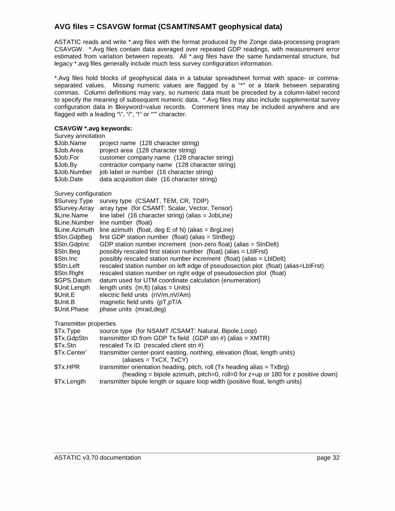
AVG files = CSAVGW format (CSAMT/NSAMT geophysical data) ASTATIC reads and write *.avg files with the format produced by the Zonge data-processing program CSAVGW. *.Avg files contain data averaged over repeated GDP readings, with measurement error estimated from variation between repeats. All *.avg files have the same fundamental structure, but legacy *.avg files generally include much less survey configuration information. *.Avg files hold blocks of geophysical data in a tabular spreadsheet format with space- or comma-separated values. Missing numeric values are flagged by a “*” or a blank between separating commas. Column definitions may vary, so numeric data must be preceded by a column-label record to specify the meaning of subsequent numeric data. *.Avg files may also include supplemental survey configuration data in $keyword=value records. Comment lines may be included anywhere and are flagged with a leading “\”, “/”, “!” or “”” character. CSAVGW *.avg keywords: Survey annotation $Job.Name project name (128 character string) $Job.Area project area (128 character string) $Job.For customer company name (128 character string) $Job.By contractor company name (128 character string) $Job.Number job label or number (16 character string) $Job.Date data acquisition date (16 character string) Survey configuration $Survey.Type survey type (CSAMT, TEM, CR, TDIP) $Survey.Array array type (for CSAMT: Scalar, Vector, Tensor) $Line.Name line label (16 character string) (alias = JobLine) $Line.Number line number (float) $Line.Azimuth line azimuth (float, deg E of N) (alias = BrgLine) $Stn.GdpBeg first GDP station number (float) (alias = StnBeg) $Stn.GdpInc GDP station number increment (non-zero float) (alias = StnDelt) $Stn.Beg possibly rescaled first station number (float) (alias = LblFrst) $Stn.Inc possibly rescaled station number increment (float) (alias = LblDelt) $Stn.Left rescaled station number on left edge of pseudosection plot (float) (alias=LblFrst) $Stn.Right rescaled station number on right edge of pseudosection plot (float) $GPS.Datum datum used for UTM coordinate calculation (enumeration) $Unit.Length length units (m,ft) (alias = Units) $Unit.E electric field units (nV/m,nV/Am) $Unit.B magnetic field units (pT,pT/A $Unit.Phase phase units (mrad,deg) Transmitter properties $Tx.Type source type (for NSAMT /CSAMT: Natural, Bipole,Loop) $Tx.GdpStn transmitter ID from GDP Tx field (GDP stn #) (alias = XMTR) $Tx.Stn rescaled Tx ID (rescaled client stn #) $Tx.Center` transmitter center-point easting, northing, elevation (float, length units)

(aliases = TxCX, TxCY) $Tx.HPR transmitter orientation heading, pitch, roll (Tx heading alias = TxBrg)

(heading = bipole azimuth, pitch=0, roll=0 for z+up or 180 for z positive down) $Tx.Length transmitter bipole length or square loop width (positive float, length units)


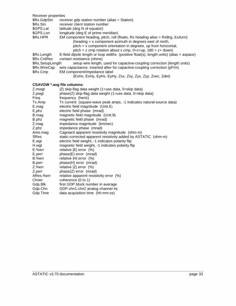
Receiver properties $Rx.GdpStn receiver gdp station number (alias = Station) $Rx.Stn receiver client station number $GPS.Lat latitude (deg N of equator) $GPS.Lon longitude (deg E of prime meridian) $Rx.HPR EM component heading, pitch, roll (floats, Rx heading alias = RxBrg, ExAzm)

(heading = x component azimuth in degrees east of north, pitch = x component orientation in degrees. up from horizontal, pitch = z cmp rotation about x cmp, 0=z+up, 180 = z+ down)

$Rx.Length E-field dipole length or loop widths (positive float(s), length units) (alias = aspace) $Rx.CntRes contact resistance (ohms) $Rx,SetupLength setup wire length, used for capactive-coupling correction (length units) $Rx.WireCap wire capacitance, inserted after for capactive-coupling correction (pF/m) $Rx.Cmp EM component/impedance label

(ExHx, ExHy, EyHx, EyHy, Zxx, Zxy, Zyx, Zyy, Zvec, Zdet) CSAVGW *.avg file columns: Z.mwgt |Z| skip-flag data weight (1=use data, 0=skip data) Z.pwgt phase(Z) skip-flag data weight (1=use data, 0=skip data) Freq frequency (hertz) Tx.Amp Tx current (square-wave peak amps, -1 indicates natural-source data) E.mag electric field magnitude (Unit.E) E.phz electric field phase (mrad) B.mag magnetic field magnitude (Unit.B) B.phz magnetic field phase (mrad) Z.mag impedance magnitude (km/sec) Z.phz impedance phase (mrad) Ares.mag Cagniard apparent resistivity magnitude (ohm-m) SRes static-corrected apparent resistivity added by ASTATIC (ohm-m) E.wgt electric field weight, -1 indicates polarity flip H.wgt magnetic field weight, -1 indicates polarity flip E.%err relative |E| error (%) E.perr phase(E) error (mrad) B.%err relative |H| error (%) B.perr phase(H) error (mrad) Z.%err relative |Z| error (%) Z.perr phase(Z) error (mrad) ARes.%err relative apparent resistivity error (%) Choer coherence (0 to 1) Gdp.Blk first GDP block number in average Gdp.Chn GDP chn1.chn2 analog channel #s Gdp.Time data acquisition time (hh:mm:ss)


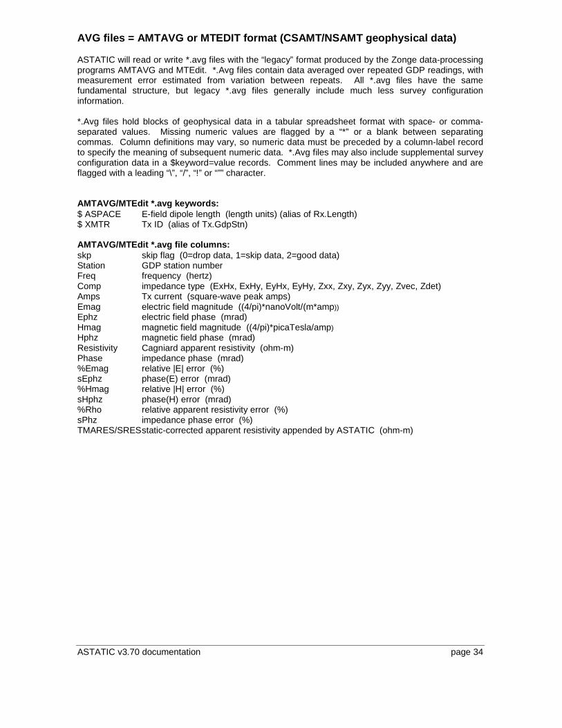
AVG files = AMTAVG or MTEDIT format (CSAMT/NSAMT geophysical data) ASTATIC will read or write *.avg files with the “legacy” format produced by the Zonge data-processing programs AMTAVG and MTEdit. *.Avg files contain data averaged over repeated GDP readings, with measurement error estimated from variation between repeats. All *.avg files have the same fundamental structure, but legacy *.avg files generally include much less survey configuration information. *.Avg files hold blocks of geophysical data in a tabular spreadsheet format with space- or comma-separated values. Missing numeric values are flagged by a “*” or a blank between separating commas. Column definitions may vary, so numeric data must be preceded by a column-label record to specify the meaning of subsequent numeric data. *.Avg files may also include supplemental survey configuration data in a $keyword=value records. Comment lines may be included anywhere and are flagged with a leading “\”, “/”, “!” or “”” character. AMTAVG/MTEdit *.avg keywords: $ ASPACE E-field dipole length (length units) (alias of Rx.Length) $ XMTR Tx ID (alias of Tx.GdpStn) AMTAVG/MTEdit *.avg file columns: skp skip flag (0=drop data, 1=skip data, 2=good data) Station GDP station number Freq frequency (hertz) Comp impedance type (ExHx, ExHy, EyHx, EyHy, Zxx, Zxy, Zyx, Zyy, Zvec, Zdet) Amps Tx current (square-wave peak amps) Emag electric field magnitude ((4/pi)*nanoVolt/(m*amp)) Ephz electric field phase (mrad) Hmag magnetic field magnitude ((4/pi)*picaTesla/amp) Hphz magnetic field phase (mrad) Resistivity Cagniard apparent resistivity (ohm-m) Phase impedance phase (mrad) %Emag relative |E| error (%) sEphz phase(E) error (mrad) %Hmag relative |H| error (%) sHphz phase(H) error (mrad) %Rho relative apparent resistivity error (%) sPhz impedance phase error (%) TMARES/SRES static-corrected apparent resistivity appended by ASTATIC (ohm-m)


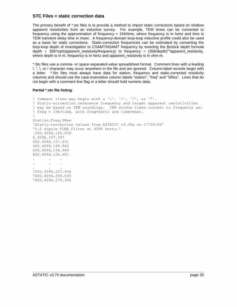
STC Files = static correction data The primary benefit of *.stc files is to provide a method to import static corrections based on shallow apparent resistivities from an inductive survey. For example, TEM times can be converted to frequency using the approximation of frequency = 194/time, where frequency is in hertz and time is TEM transient delay time in msec. A frequency-domain loop-loop inductive profile could also be used as a basis for static corrections. Static-correction frequencies can be estimated by converting the loop-loop depth of investigation to CSAMT/NSAMT frequency by inverting the Bostick depth formula depth = 356*sqrt(apparent_resistivity/frequency) to frequency = (356/depth)2*apparent_resistivity, where depth is in m, frequency is in hertz and apparent_resistivity is in ohm-m. *.Stc files use a comma- or space-separated-value spreadsheet format. Comment lines with a leading !, “, \, or / character may occur anywhere in the file and are ignored. Column-label records begin with a letter. *.Stc files must always have data for station, frequency and static-corrected resistivity columns and should use the case-insensitive column labels “station”, “freq” and “SRes”. Lines that do not begin with a comment line flag or a letter should hold numeric data. Partial *.stc file listing: ! Comment lines may begin with a ‘\’, ‘/’, ‘!’, or ‘”’. \ Static-correction reference frequency and target apparent resistivities \ may be based on TEM soundings. TEM window times convert to frequency as: \ freq = 194/time, with freq=hertz and time=msec. \ Station,Freq,SRes "Static-correction values from ASTATIC v3.30a on 17 /04/06" "5.0 dipole FLMA Filter at 4096 hertz." -200,4096,160.059 0,4096,157.347 200,4096,157.031 400,4096,149.962 600,4096,136.969 800,4096,126.601 . . . . . . . . . 7200,4096,237.936 7400,4096,258.035 7600,4096,279.364


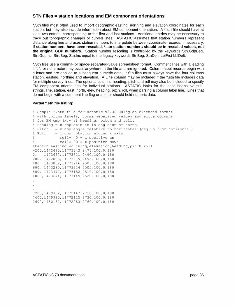
STN Files = station locations and EM component orientations *.Stn files most often used to import geographic easting, northing and elevation coordinates for each station, but may also include information about EM component orientation. A *.stn file should have at least two entries, corresponding to the first and last stations. Additional entries may be necessary to trace out topographic changes or curved lines. ASTATIC assumes that station numbers represent distance along line and uses station numbers to interpolate between coordinate records, if necessary. If station numbers have been rescaled, *.stn station numbers should be in rescaled values, not the original GDP numbers. Station number rescaling is controlled by the keywords Stn.GdpBeg, Stn.GdpInc, Stn.Beg, Stn.Inc equal to the legacy keywords StnBeg, StnDelt, LblFrst LblDelt. *.Stn files use a comma- or space-separated-value spreadsheet format. Comment lines with a leading !, “, \, or / character may occur anywhere in the file and are ignored. Column-label records begin with a letter and are applied to subsequent numeric data. *.Stn files must always have the four columns station, easting, northing and elevation. A Line column may be included if the *.stn file includes data for multiple survey lines. The optional columns heading, pitch and roll may also be included to specify EM component orientations for individual stations. ASTATIC looks for the case-insensitive sub-strings, line, station, east, north, elev, heading, pitch, roll, when parsing a column label line. Lines that do not begin with a comment line flag or a letter should hold numeric data. Partial *.stn file listing: ! Sample *.stn file for astatic v3.30 using an exte nded format ! with column labels, comma-separated values and ex tra columns ! for EM cmp (x,y,z) heading, pitch and roll. ! Heading = x cmp azimuth in deg east of north. ! Pitch = x cmp angle relative to horizontal (deg up from horizontal) ! Roll = z cmp rotation around x axis ! roll= 0 = z positive up ! roll=180 = z positive down station,easting,northing,elevation,heading,pitch,ro ll -200,1472490,11773343,2475,100,0,180 0, 1472687,11773311,2490,100,0,180 200, 1472885,11773279,2495,100,0,180 400, 1473082,11773246,2505,100,0,180 600, 1473280,11773214,2505,100,0,180 800, 1473477,11773182,2510,100,0,180 1000,1473674,11773149,2520,100,0,180 . . . . . . . . . 7200,1479792,11772147,2718,100,0,180 7400,1479990,11772115,2730,100,0,180 7600,1480187,11772083,2760,100,0,180


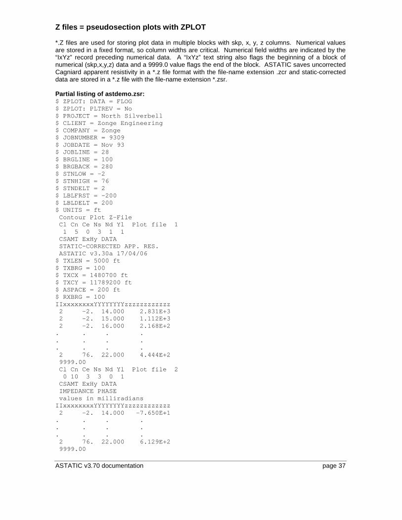
Z files = pseudosection plots with ZPLOT *.Z files are used for storing plot data in multiple blocks with skp, x, y, z columns. Numerical values are stored in a fixed format, so column widths are critical. Numerical field widths are indicated by the “IxYz” record preceding numerical data. A “IxYz” text string also flags the beginning of a block of numerical (skp,x,y,z) data and a 9999.0 value flags the end of the block. ASTATIC saves uncorrected Cagniard apparent resistivity in a *.z file format with the file-name extension .zcr and static-corrected data are stored in a *.z file with the file-name extension *.zsr. Partial listing of astdemo.zsr: $ ZPLOT: DATA = FLOG $ ZPLOT: PLTREV = No $ PROJECT = North Silverbell $ CLIENT = Zonge Engineering $ COMPANY = Zonge $ JOBNUMBER = 9309 $ JOBDATE = Nov 93 $ JOBLINE = 28 $ BRGLINE = 100 $ BRGBACK = 280 $ STNLOW = -2 $ STNHIGH = 76 $ STNDELT = 2 $ LBLFRST = -200 $ LBLDELT = 200 $ UNITS = ft Contour Plot Z-File Cl Cn Ce Ns Nd Yl Plot file 1 1 5 0 3 1 1 CSAMT ExHy DATA STATIC-CORRECTED APP. RES. ASTATIC v3.30a 17/04/06 $ TXLEN = 5000 ft $ TXBRG = 100 $ TXCX = 1480700 ft $ TXCY = 11789200 ft $ ASPACE = 200 ft $ RXBRG = 100 IIxxxxxxxxYYYYYYYYzzzzzzzzzzzz 2 -2. 14.000 2.831E+3 2 -2. 15.000 1.112E+3 2 -2. 16.000 2.168E+2 . . . . . . . . . . . . 2 76. 22.000 4.444E+2 9999.00 Cl Cn Ce Ns Nd Yl Plot file 2 0 10 3 3 0 1 CSAMT ExHy DATA IMPEDANCE PHASE values in milliradians IIxxxxxxxxYYYYYYYYzzzzzzzzzzzz 2 -2. 14.000 -7.650E+1 . . . . . . . . . . . . 2 76. 22.000 6.129E+2 9999.00

Documents

ASTATIC Documentation - Zonge International · ASTATIC v3.70 documentation page 5 Geographic coordinates are specified as eastings, northings and elevation rather than x, y, z to