ASTRONOMICAL STATISTICS

Andy TaylorRoom C19, Royal Observatory; ant@roe.ac.uk

December 17, 2004

Contents

1 PROBABILITY AND STATISTICS 41.1 Introduction . . . . . . . . . . . . . . . . . . . . . . . . . . . . . . . . . . . 41.2 What is a probability ? . . . . . . . . . . . . . . . . . . . . . . . . . . . . . 51.3 The calculus of probability . . . . . . . . . . . . . . . . . . . . . . . . . . . 71.4 Moments of the distribution . . . . . . . . . . . . . . . . . . . . . . . . . . 81.5 Discrete probability distributions . . . . . . . . . . . . . . . . . . . . . . . 9

1.5.1 Binomial Distribution . . . . . . . . . . . . . . . . . . . . . . . . . 91.5.2 The Poisson distribution . . . . . . . . . . . . . . . . . . . . . . . . 111.5.3 Moments of the Poisson distribution: . . . . . . . . . . . . . . . . . 121.5.4 A rule of thumb . . . . . . . . . . . . . . . . . . . . . . . . . . . . . 131.5.5 Detection of a Source . . . . . . . . . . . . . . . . . . . . . . . . . . 131.5.6 Testing the Isotropy of the Universe . . . . . . . . . . . . . . . . . . 131.5.7 Identifying Sources . . . . . . . . . . . . . . . . . . . . . . . . . . . 14

1.6 Continuous probability distributions . . . . . . . . . . . . . . . . . . . . . . 151.6.1 The Gaussian Distribution . . . . . . . . . . . . . . . . . . . . . . . 151.6.2 Transformation of random variables . . . . . . . . . . . . . . . . . . 161.6.3 An example: projection of a random pencil . . . . . . . . . . . . . . 161.6.4 The predicted distribution of superluminal velocities in quasars. . . 17

1.7 The addition of random variables . . . . . . . . . . . . . . . . . . . . . . . 191.7.1 Multivariate distributions and marginalisation . . . . . . . . . . . . 191.7.2 The probability distribution of summed random variables . . . . . . 191.7.3 Error propagation . . . . . . . . . . . . . . . . . . . . . . . . . . . . 20

1.8 Characteristic functions . . . . . . . . . . . . . . . . . . . . . . . . . . . . 211.9 The Central Limit Theorem . . . . . . . . . . . . . . . . . . . . . . . . . . 23

1.9.1 Derivation of the central limit theorem . . . . . . . . . . . . . . . . 231.9.2 Measurement theory . . . . . . . . . . . . . . . . . . . . . . . . . . 241.9.3 How the Central Limit Theorem works . . . . . . . . . . . . . . . . 25

1.10 Sampling distributions . . . . . . . . . . . . . . . . . . . . . . . . . . . . . 261.10.1 The sample variance . . . . . . . . . . . . . . . . . . . . . . . . . . 261.10.2 Measuring quasar variation . . . . . . . . . . . . . . . . . . . . . . 28

2 STATISTICAL INFERENCE 292.1 Model fitting and parameter estimation . . . . . . . . . . . . . . . . . . . 29

2.1.1 The method of least-squares fits . . . . . . . . . . . . . . . . . . . . 292.1.2 Estimating a mean from Least Squares . . . . . . . . . . . . . . . . 31

1

2.1.3 Multiparameter estimation . . . . . . . . . . . . . . . . . . . . . . . 312.1.4 Goodness of fit . . . . . . . . . . . . . . . . . . . . . . . . . . . . . 332.1.5 A rule of thumb for goodness of fit . . . . . . . . . . . . . . . . . . 332.1.6 Confidence regions for minimum χ2 . . . . . . . . . . . . . . . . . . 34

2.2 Maximum Likelihood Methods . . . . . . . . . . . . . . . . . . . . . . . . . 362.2.1 The flux distribution of radio sources . . . . . . . . . . . . . . . . . 362.2.2 Goodness-of-fit and confidence regions from maximum likelihood . . 372.2.3 Estimating parameter uncertainty . . . . . . . . . . . . . . . . . . . 38

2.3 Hypothesis testing . . . . . . . . . . . . . . . . . . . . . . . . . . . . . . . 382.3.1 Introduction . . . . . . . . . . . . . . . . . . . . . . . . . . . . . . . 382.3.2 Bayes Theorem . . . . . . . . . . . . . . . . . . . . . . . . . . . . . 392.3.3 Updating the probability of a hypothesis . . . . . . . . . . . . . . . 392.3.4 The prior distribution . . . . . . . . . . . . . . . . . . . . . . . . . 40

2.4 Imaging process and Bayes’ Theorem . . . . . . . . . . . . . . . . . . . . . 412.4.1 Using the prior . . . . . . . . . . . . . . . . . . . . . . . . . . . . . 412.4.2 Maximum Entropy . . . . . . . . . . . . . . . . . . . . . . . . . . . 42

2.5 Non-parametric statistics . . . . . . . . . . . . . . . . . . . . . . . . . . . . 432.5.1 The χ2-goodness-of-fit test . . . . . . . . . . . . . . . . . . . . . . . 432.5.2 The Kolmogorov-Smirnov test . . . . . . . . . . . . . . . . . . . . . 452.5.3 The Spearman rank correlation coefficient . . . . . . . . . . . . . . 45

2.6 Inference from correlations . . . . . . . . . . . . . . . . . . . . . . . . . . . 482.6.1 Other Malmquist sampling effects . . . . . . . . . . . . . . . . . . . 502.6.2 Example: Malmquist bias in a quasar survey . . . . . . . . . . . . . 51

2.7 Monte-Carlo Methods . . . . . . . . . . . . . . . . . . . . . . . . . . . . . 52

2

Suggested references:

Textbooks on probability and statistics are notoriously: (a) boring (b) irrelevant toastronomers and physicists (c) from one viewpoint and ignore others (d) all of the above.Given this the main text for this course is these notes. However if you’re after more, twotext that do much better than the norm are:

• Robert Lupton, Statistics in Theory and Practice, Princeton University Press;ISBN: 0691074291, Price: 29.95 (from Amazon). This is a great textbook, verymuch in the vein of this course. Good intro.

• William H. Press, Brian P. Flannery, Saul A. Teukolsky, William T. Vetterling,Numerical Recipes in FORTRAN Example Book: The Art of Scientific Computing,Cambridge University Press; ISBN: 0521437210, Price: 22.95 (from Amazon). Thiscovers much more than statistics, and provides computer code for all its methods.There is a C and C++ version if you’re not into Fortran. Apart from actual code,its strength is in clear explanations of scientific methods, in particular StatisticalMethods.

3

PART ONE

1 PROBABILITY AND STATISTICS

1.1 Introduction

Science, and in particular Modern Astronomy and Astrophysics, is impossible withoutknowledge of probability and statistics. To see this let’s consider how Scientific Knowl-edge evolves1. First of all we start with a problem, e.g., a new observation, or somethingunexplained in an existing theory. In the case of a new observation, probability and statis-tics are already required to make sure we are have detected something at all. We thenconjecture (or rather we simply make up) a set of solutions, or theories, explaining theproblem. Hopefully these theories can be used to deduce testable predictions (or theyare not much use), so that they can be experimentally tested. The predictions can beof a statistical nature, i.e., the mean value of a property of a population of objects orevents. We then need probability and statistics to help us decide which theories pass thetest and which do not. Even in everyday situations we have to make such decisions, whenwe do not have complete certainty. If we are sure a theory has failed the test it can bedisregarded, and if it passes it lives to fight another day. We cannot “prove” a theorytrue, since we don’t know if it will fail a critical test tomorrow.

In all of this probability and statistics are vital for:

• Detection of signals:How do we know if we’ve found a new object or detected a new signal?e.g. detection of astronomical objects, detection of spectral features, detection of fluctu-

ations in temperature or polarisation in the microwave background, detection of galaxy

clustering.

• Detection of correlations:A correlation between two quantities may imply a physical connection. But how dowe detect any such correlation? And when should we believe its real?e.g. Hubble diagram, the Hertsprung-Russell diagram, galaxy colour-magnitude relations.

• Tests of hypotheses:How do we rule out a false theory? Or pass another ?e.g. isotropy of the Universe, physical association between astronomical objects, the exis-

tence and nature of dark matter and dark energy in the Universe.

• Model-fitting to data and interpretation:How should we compare our models with data?e.g. compare a cosmological theory with the cosmic microwave background or galaxy

redshift survey, or compare a stellar model with the observed solar neutrino flux.

• Estimation of parameters:If a model does fit the data, how do we extract estimates of the model parametersthat best fit the data?

1from the Theory of Knowledge, by Karl Popper in Conjecture and Refutations, 1963.

4

e.g. the mean mass density of the Universe, the temperature, surface gravity, metallicity

of stars, number and mass of neutrinos.

• As a theoretical tool:How do we model or predict the properties of populations of objects, or studycomplex systems?e.g. Statistical properties of galaxy populations, or stars, simulations of stellar clusters or

large-scale structure, turbulence in the IGM.

In astronomy the need for statistical methods is especially acute, as we cannot directlyinteract with the objects we observe. For instance, we can’t re-run the same supernovaover and again, from different angles and with different initial conditions, to see whathappens. Instead we have to assume that by observing a large number of such events, wecan collect a “fair sample”, and draw conclusions about the physics of supernovae fromthis sample. Without this assumption, that we can indeed collect fair samples, it wouldbe questionable if astronomy is really a science. This is also an issue for other subjects,such as archeology or forensics. As a result of this strong dependence on probabilisticand statistical arguments, many astronomers have contributed to the development ofprobability and statistics.

As a result, there are strong links between the statistical methods used in astronomyand those used in many other areas. These include particularly any science that makesuse of signals (e.g. speech processing) or images (e.g. medical physics) or of statisticaldata samples (e.g. psychology). And in the real world, of course, statistical analysis isused for a wide range of purposes from forensics, risk assessment, economics and, its firstuse, in gambling.

1.2 What is a probability ?

The question “what is a probability?” is actually a very tricky one. Surprisingly thereisn’t a universally agreed definition. The answer to the question “What is a probability?”depends on how you assign probabilities in the first place. To understand the origins ofthis problem let’s take a quick look at the historical development of probability:

1654: Blaise Pascal & Pierre Fermat: After being asked by an aristocratic professionalgambler how the stakes should be divided between players in a game of chance ifthey quit before the game ends, Pascal (he of the triangle) and Fermat (of ‘LastTheorem’ fame) began a correspondence on how to make decisions in situations inwhich it is not possible to argue with certainty, in particular for gambling probabil-ities. Together, in a series of letters in 1654, they laid down the basic Calculus ofProbabilities (See Section 1.3).

1713: James (Jacob) Bernoulli: Bernoulli was the first to wonder how does one assigna probability. He developed the “Principle of Insufficient Reason”: if there areN events, and no other information, one should assign each event the probabilityP = 1/N . But he then couldn’t see how one should update a probability after anevent has happened.

5

1763: Thomas Bayes: Edinburgh, 1763, and the Rev. Thomas Bayes solved Bernoulli’sproblem of how to update the probability of an event (or hypothesis) given newinformation. The formula that does this is now called “Bayes’ Theorem” (seeSection 2.3).

1795: Johann Friederich Carl Gauss: At the age of 18, the mathematical astronomer,Gauss, invented the method of ‘Least Squares’ (section 2.1), derived the Gaussiandistribution of errors (section 1.6), and formulated the Central Limit Theorem (sec-tion 1.9).

1820: Pierre-Simon de Laplace: Another mathematical astronomer, Laplace re-discoveredBayes’ Theorem and applied it to Celestial Mechanics and Medical Statistics. Markeda return to earlier ideas that “probability” is a lack of information

1850’s: The Frequentists: Mathematicians rejected Laplace’s developments and try toremove subjectivity from the definition of probability. A probability is a measuredfrequency. To deal with everyday problems they invent Statistics. Notable amongstthese are Boole (1854), Venn (of Diagram fame) (1888), Fisher (1932) and von Mises(1957).

1920’s: The Bayesians: We see a return to the more intuitive ideas of Bayes and Laplacewith the “Neo-Bayesian”. A probability is related to the amount of informationwe have to hand. This began with John Maynard Keynes (1921), and continuedwith Jeffreys (1939), Cox (1946) and Steve Gull (1980).

1989: E. Jaynes: Using Bayesian ideas Jaynes tries to solve the problem of assigningprobability with the “Principle of Maximum Entropy” (section 2.4).

So what is a probability ? There are two basic philosophies about what a probabilityis, based on how the probabilities are assigned:

• Frequentist (or Classical) probabilities: Probabilities are measureable frequen-cies, assigned to objects or events. In some situations, e.g., for single events, or insituations were we cannot in practice measure the frequency, we have to invent ahypothetical ensemble of events.

• Bayesian probabilities: Probability is a “degree-of-belief” of the outcome of anevent, allocated by an observer given the available evidence. While this is moreintuitive it can lead to problems with subjectivity. But if all observers have the sameevidence and allocate the same probability, Bayesians would argue it is objective.

These do not obviously give the same answer to problems in probability and statistic,as they assign different probabilities to some events. However, in many instances theyare the same, and both agree on the basics of probability theory (see next section). Inthis course we shall mostly work in the Frequentist framework, since the majority ofprobability and statistics has been formulated this way. This should provide a “toolbox”of practical methods to solve everyday problems in physics and astronomy. However, weshall encounter situations where we are forced to consider the Bayesian approach, and itsdeep implications.

6

1.3 The calculus of probability

The Calculus of Probabilities is the mathematical theory which allows us to predictthe statistical behaviour of complex systems from a basic set of fundamental axioms.Probabilities come in two distinct forms: discrete, where Pi is the probability of the ith

event occurring, and continuous, where P (x) is the probability that the even, or randomvariable, x, occurs.

1. The Range of Probabilities: The probability of an event is measurable on acontinuous scale, such that P (x) is a real number in the range 0 ≤ P (x) ≤ 1.

2. The Sum Rule: The sum of all discrete possibilities is∑

i

Pi = 1. (1)

For a continuous range of random variables, x, this becomes∫ ∞

−∞dx p(x) = 1, (2)

where p(x) is the probability density. The probability density clearly must haveunits of 1/x.

3. The Addition of Exclusive Probabilities: If the probabilities of n mutuallyexclusive events, x1, x2 · · · xn are P (x1), P (x2) · · ·P (xn), then the probability thateither x1 or x2 or · · · xn occurs is2

P (x1 + x2 + · · · + xn) = P (x1) + P (x2) + · · · + P (xn) (3)

4. The Multiplication of Probabilities: The probability of two events x and yboth occurring is the product of the probability of x occurring and the probabilityof y occurring given that x has occurred. In notational form:

P (x, y) = P (x|y)P (y)

= P (y|x)P (x) (4)

where we have introduced the conditional probability, P (x|y), which denotesthe probability the of x given the event y has occurred. If x and y are independentevents then

P (x, y) = P (x)P (y). (5)

Problem 1.1Three coins are tossed. What is the probability that they fall either all heads or all tails?(Assume P (heads) = P (tail) = 1/2). Try some of these suggested answers:

1. There are 8 possible equally probable combinations (HHH, HHT, HTH,......). Twoof these give us either all heads or all tails, so the probability is 1/4.

2Maths Notes: The logical proposition “A.OR.B” can be written as A + B, or in set theory,

A⋃

B,which is the union of the set of events A and B. Similarly “A.AND.B” can be written as AB orA⋂

B, which is the intersection of events.

7

2. There are 2 possibilities: either all 3 coins fall alike, or 2 fall alike and 1 is different.Hence the probability is 1/2.

3. There are 4 possibilities: 3 heads, 2 heads and 1 tail, 2 tails and 1 head, 3 tails.Hence the probability is 2/4 = 1/2.

4. Of the 3 coins, 2 must fall alike. The other must either be the same as these ordifferent, so probability is 1/2. Which of these arguments are wrong, and why?

1.4 Moments of the distribution

Probability distributions can be characterized by their moments.

Definition:mn ≡ 〈xn〉 =

∫ ∞

−∞dx xnp(x), (6)

is the nth moment of a distribution. The angled brackets 〈· · ·〉 denote the expectationvalue. Probability distributions are normalized so that

m0 =∫ ∞

−∞dx p(x) = 1 (7)

(Axiom 2, The Sum Rule).

The first moment,m1 = 〈x〉, (8)

gives the expectation value of x, called the mean: the average or typical expected valueof the random variable x if we make random drawings from the probability distribution.

Centred moments are obtained by shifting the origin of x to the mean;

µn ≡ 〈(x − 〈x〉)n〉. (9)

The second centred moment,

µ2 = 〈(x − 〈x〉)2〉, (10)

is a measure of the spread of the distribution about the mean. This is such an importantquantity it is often called the variance, and denoted

σ2 ≡ µ2. (11)

We will need the following, useful result later:

σ2 = 〈(x − 〈x〉)2〉 = 〈(x2 − 2x〈x〉 + 〈x〉2)〉 = 〈x2〉 − 〈x〉2. (12)

The variance is obtained from the mean of the square minus the square of the mean. An-other commonly defined quantity is the square-root of the variance, called the standard

8

deviation; σ. This quantity is sometimes also called the root mean squared (rms)deviation3, or error4.

Higher moments characterise the distribution further, with odd moments characteris-ing asymmetry. In particular the third moment, called the skewness, 〈x3〉, characterisesthe simplest asymmetry, while the fourth moment, the kurtosis, 〈x4〉, characterises theflatness of the distribution. Rarely will one go beyond these moments.

For bivariate distributions (of two random variables), p(x, y), one can also define acovariance (assume 〈x〉 = 〈y〉 = 0);

Cov(x, y) = 〈xy〉 =∫ ∞

−∞dx dy xy p(x, y) (13)

and a dimensionless correlation coefficient;

r =〈xy〉

√

〈x2〉〈y2〉, (14)

which quantifies the similarity between two variables. r must lies between +1 (completelycorrelated) and −1 (completely anti-correlated). r = 0 indicates the variables are uncor-related (but not necessarily independent). We shall meet the correlation coefficient laterwhen we try and estimate if two data sets are related.

1.5 Discrete probability distributions

We can use the calculus of probabilities to produce a mathematical expression for theprobability of a wide range of multiple events such as discussed in Example 1.

1.5.1 Binomial Distribution

The Binomial distribution allows us to calculate the probability, Pn, of n suc-cesses arising after N independent trials.

Suppose we have a sample of objects of which a probability, p1, of have some attribute(such as a coin being heads-up) and a probability, p2 = 1−p1 of not having this attribute(e.g. tails-up). Suppose we sample these objects twice, e.g. toss a coin 2 times, or toss 2coins at once. The possible out comes are hh, ht, th, and tt. As these are independentevents we see that the probability of each distinguishable outcome is

P (hh) = P (h)P (h),

P (ht + th) = P (ht) + P (th) = 2P (h)P (t),

P (tt) = P (t)P (t). (15)

3One should be cautious, as the term rms need not apply to deviations from the mean. It sometimesapplies to

√m2. One should be explicit that it is a rms deviation, unless the mean is known to be zero.

4Again one should be cautions about referring to σ as the error. ‘Error’, or ‘uncertainty’ implies thedistribution has a Gaussian form (see later), which in general is untrue.

9

These combinations are simply the coefficients of the binomial expansion of the quan-tity (P (h) + P (t))2. In general, if we draw N objects, then the number of possiblepermutations which can result in n of them having some attribute is the nth coefficient inthe expansion of (p1 + p2)

N , the probability of each of these permutations is pn1p

N−n2 , and

the probability of n objects having some attribute is the binomial expansion

Pn = CNn pn

1pN−n2 , (0 ≤ n ≤ N), (16)

where

CNn =

N !

n!(N − n)!(17)

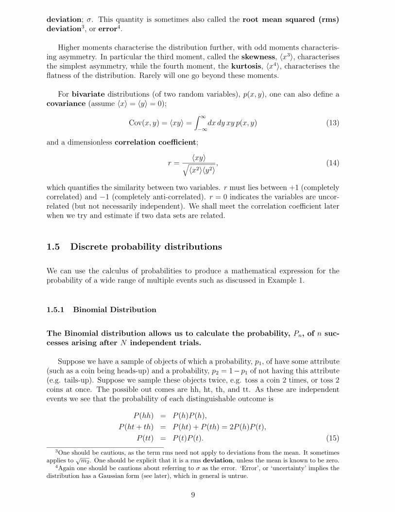
are the Binomial coefficients. The binomial coefficients can here be viewed as statisticalweights which allow for the number of possible indistinguishable permutations which leadto the same outcome. This distribution is called the general Binomial, or Bernoullidistribution. We can plot out the values of Pn for all the possible n (Figure 1) and in

Figure 1: Histogram of a binomial distribution

doing so have generated the predicted probability distribution which in this case is thebinomial distribution whose form is determined by N , n, p1. If we have only two possibleoutcomes p2 = 1 − p1. The Binomial distribution can be generalised to a multinomialdistribution function.

The mean of the binomial distribution is

〈n〉 =N∑

n=0

nP

=N∑

n=0

nN !

n!(N − n)!pn

1pN−n2

=N∑

n=1

N !

(n − 1)!(N − n)!pn

1pN−n2

=N∑

n=1

N(N − 1)!

(n − 1)!(N − n)!p1p

n−11 pN−n

2

= Np1 (18)

10

For p1 6= p2 the distribution is asymmetric, with mean 〈n〉 = Np1, but if is large theshape of the envelope around the maximum looks more and more symmetrical and tendstowards a Gaussian distribution - an example of the Central Limit Theorem at work.More of this later!

1.5.2 The Poisson distribution

The Poisson distribution occupies a special place in probability and statistics, andhence in observational astronomy. It is the archetypical distribution for point processes.It is of particular importance in the detection of astronomical objects since it describesphoton noise. It essentially models the distribution of randomly distributed, indepen-dent, point-like events, and is commonly taken as the null hypothesis.

It can be derived as a limiting form of the binomial distribution:

The probability of n “successes” of an event of probability p is

Pn = CNn pn(1 − p)N−n (19)

after N trials.

Let us suppose that the probability p is very small, but that in our experiment weallow N to become large, while keeping the mean finite, so that we have a reasonablechance of finding a finite number of successes n. That is we define λ = 〈n〉 = Np and letp → 0, N → ∞, while λ =constant. Then,

Pn =N !

n!(N − n)!

(

λ

N

)n (

1 − λ

N

)N−n

(20)

Using Stirling’s approximation, where x! →√

2πe−xxx+1/2 when x → ∞, and lettingN → ∞, we find5

N !

(N − n)!=

√2πe−NNN+1/2

√2πe−(N−n)(N − n)N−n+1/2

=e−nNN+1/2

NN−n+1/2(1 − n/N)N−n+1/2

= e−nNnen

= Nn (22)

and(

1 − λ

N

)N−n

= e−λ. (23)

5Maths Note The limit of terms like (1 − x/N)N when N → ∞ can be found by taking the natural

log and expanding to first order:

N ln(1 − x/N) → N(−x/N) = −x (21)

11

Combining these results with equation (20) we find

Pn =λne−λ

n!(24)

This is Poisson’s distribution for random point processes, discovered by him in1837.

1.5.3 Moments of the Poisson distribution:

Let’s look at the moments of the Poisson distribution:

mi = 〈ni〉 =∞∑

n=0

niPn (25)

The mean of Poisson’s distribution is

〈n〉 =∞∑

n=0

nλne−λ

n!

=∞∑

n=1

λne−λ

(n − 1)!

=∞∑

n=1

λλn−1e−λ

(n − 1)!

= λ (26)

i.e. the expectation value of Poisson’s distribution is the factor λ. This makes sense sinceλ was defined as the mean of the underlying Binomial distribution, and kept constantwhen we took the limit. Now lets look at the second centred moment (i.e. the variance):

µ2 =∞∑

n=0

(n − 〈n〉)2λne−λ

n!

=∞∑

n=0

n2 λne−λ

n!− λ2

=∞∑

n=1

nλne−λ

(n − 1)!− λ2

=∞∑

n=1

nλλn−1e−λ

(n − 1)!− λ2

=∞∑

n=0

(n + 1)λλne−λ

n!− λ2

= (λ + 1)λ − λ2

= λ. (27)

So the variance of Poisson’s distribution is also λ. This means that the variance ofthe Poisson distribution is equal to its mean. This is a very useful result.

12

1.5.4 A rule of thumb

Lets see how useful this result is. When counting photons, if the expected number detectedis n, the variance of the detected number is n: i.e. we expect typically to detect

n ±√

n (28)

photons. Hence, just by detecting n counts, we can immediately say that the uncertaintyon that measurement is ±√

n, without knowing anything else about the problem, andonly assuming the counts are random. This is a very useful result, but beware: whenstating an uncertainty like this we are assuming the underlying distribution is Gaussian(see later). Only for large n does the Poisson distribution look Gaussian (the CentralLimit Theorem at work again), and we can assume the uncertainty σ =

√n.

1.5.5 Detection of a Source

A star produces a large number, N 1, of photons during its life. If we observe it with atelescope on Earth we can only intercept a tiny fraction, p 1, of the photons which areemitted in all directions by the star, and if we collect those photons for a few minutes orhours we will collect only a tiny fraction of those emitted throughout the life of the star.

So if the star emits N photons in total and we collect a fraction, p, of those, then

λ = Np

N → ∞p → 0. (29)

So if we make many identical observations of the star and plot out the frequency dis-tribution of the numbers of photons collected each time, we expect to see a Poissondistribution.

Conversely, if we make one observation and detect n photons, we can use the Poissondistribution to derive the probability of all the possible values of λ: we can set confidencelimits on the value of λ from this observation. And if we can show that one piece ofsky has only a small probability of having a value of λ as low as the surrounding sky,then we can say that we have detected a star, quasar, galaxy or whatever at a particularsignificance level (i.e. at a given probability that we have made a mistake due to therandom fluctuations in the arrival rate of photons). A useful rule of thumb here is

λS ≥ λB + ν√

λB (30)

where λS is the mean counts from the source, λB, is the mean background count, and νis the detection level. Usually we take ν = 3 to be a detection, but sometimes it can beν = 5 or even ν = 15 for high confidence in a detection.

1.5.6 Testing the Isotropy of the Universe

A key observation in cosmology is that the universe appears isotropic on large scales.Unless our galaxy occupies an extremely special place in the universe, then isotropy

13

implies homogeneity. Without this information a wide range of different cosmologicalmodels become possible, and homogeneity pins down the type of universe we inhabit andthe manner in which it evolves.

But how do we test for isotropy? Let us suppose that we count a large number ofquasars in many different parts of the sky to obtain an average surface density of quasars,per square degree. Dr. Anne Isotropy6 is investigating quasar counts in one area of skyand finds an unusually large number of quasars, n in her area of one square degree. Doesthis indicate anisotropy or is it a random fluctuation?

The probability of finding exactly n quasars is

Pn =λne−λ

n!. (31)

But being an astronomer of integrity, she admits that she would have been equally excitedif she had found any number greater than the observed number n. So the probability ofobtaining N quasars or greater is

P (≥ N) =∞∑

n=N

λne−λ

n!. (32)

If λ = 2 and N = 5, PN = 0.036 but P (N ≥ 5) ≈ 0.053; i.e. there is only a 5% chance ofsuch a fluctuation occurring at random.

But nobody believes her result is significant, because it turns out that she had searchedthrough 20 such fields before finding her result, and we should expect one out of those20 to show such a fluctuation. The more she looks for anisotropy, the more stringent hercriteria have to be!

P (≥ N) has a particularly simple form if N = 1:

P (≥ 1) =∞∑

n=1

λne−λ

n!

= 1 − e−λ. (33)

Hence for λ 1, P (n ≥ 1) → λ. The function P (≥ N) is called the cumulativeprobability distribution.

1.5.7 Identifying Sources

Suppose we are trying to find the optical counterpart to a known X-ray source, whoseposition is known to some finite accuracy: we say that we know the size of the X-ray errorbox (usually this will be a circle!). We attempt to do this by looking within that errorbox on an optical image of the same region of sky. We know from counting the numberof stars etc. on that image the number of chance coincidences that we expect within theerror box, λ, and we can use this information to decide whether or not the existence ofan optical object close to the X-ray source is evidence that the two are related. If λ = 1

6Sorry...

14

then the probability of finding one or more chance coincidences is 63 percent: this tellsus that if we want to rely on this information alone we cannot expect our identificationto be very reliable in this example.

1.6 Continuous probability distributions

So far we have dealt with discrete probability distributions (e.g. number of heads, numberof photons, number of quasars). But in other problems we wish to know the probabilitydistribution of a quantity which is continuously variable (e.g. the angle θ between twodirections can have any real value between 0 and 360). We can define a function θ suchthat the probability that the quantity θ has values between θ − dθ/2 and θ + dθ/2 isP (θ)|dθ|, and the probability that has any value larger than is

p(θ ≥ θ1) =∫ 2π

θ1

dθ p(θ) (34)

The quantity θ is known as a random variable and is used to denote any possible valueswhich a quantity can have. Here p(θ) called the probability density. If its argumenthas dimensions, the probability density will be measured in units of inverse dimensions.p(θ ≥ θ1) is again called the cumulative probability distribution, and is dimensionless.

1.6.1 The Gaussian Distribution

A limiting form of the Poisson distribution (and most others - see the Central LimitTheorem below) is the Gaussian distribution. Let’s write the Poisson distribution as

Pn =λne−λ

n!(35)

Now let x = n = λ(1 + δ) where λ 1 and δ 1. Using Stirlings formula for n! wefind7

p(x) =λλ(1+δ)e−λ

√2πe−λ(1+δ)[λ(1 + δ)]λ(1+δ)+1/2

=eλδ(1 + δ)−λ(1+δ)

√2πλ

=e−λδ2/2

√2πλ

(37)

Substituting back for x yields

p(x) =e−(x−λ)2/(2λ)

√2πλ

(38)

7Maths Notes: The limit of a function like (1 + δ)λ(1+δ) with λ 1 and δ 1 can be found by

taking the natural log, then expanding in δ to second order (first order will cancel later):

−λ(1 + δ) ln(1 + δ) = −λ(1 + δ)(δ − δ2/2) = −λδ(1 + δ/2). (36)

15

This is a Gaussian, or Normal8, distribution with mean and variance of λ. The Gaussiandistribution is the most important distribution in probability, due to its role in the CentralLimit Theorem. It is also one of the simplest.

1.6.2 Transformation of random variables

The probability that a random variable x has values in the range x − dx/2 to x + dx/2is just p(x)dx. Remember p(x) is the probability density. We wish to transform theprobability distribution p(x) to the probability distribution g(y), where y is a function ofx. For a continuous function we can write,

p(x)dx = g(y)dy. (39)

This just states that probability is a conserved quantity, neither created nor destroyed.Hence

p(x) = g(y(x))

∣

∣

∣

∣

∣

dy

dx

∣

∣

∣

∣

∣

. (40)

So the transformation of probabilities is just the same as the transformation of normalfunctions in calculus. This was not necessarily obvious, since a probability is a specialfunction of random variables. This transformation is of great importance in astronomicalstatistics. For example it allows us to transform between distributions and variables thatare useful for theory, and those that are observed.

1.6.3 An example: projection of a random pencil

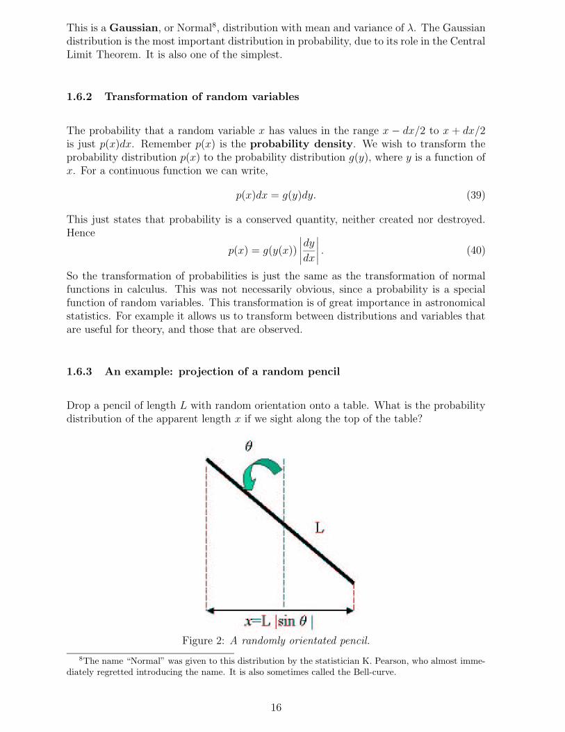
Drop a pencil of length L with random orientation onto a table. What is the probabilitydistribution of the apparent length x if we sight along the top of the table?

Figure 2: A randomly orientated pencil.

8The name “Normal” was given to this distribution by the statistician K. Pearson, who almost imme-diately regretted introducing the name. It is also sometimes called the Bell-curve.

16

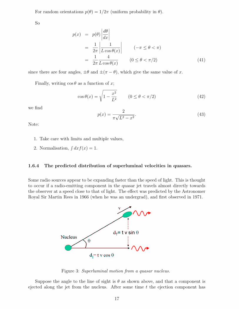
For random orientations p(θ) = 1/2π (uniform probability in θ).

So

p(x) = p(θ)

∣

∣

∣

∣

∣

dθ

dx

∣

∣

∣

∣

∣

=1

2π

∣

∣

∣

∣

∣

1

L cos θ(x)

∣

∣

∣

∣

∣

(−π ≤ θ < π)

=1

2π

4

L cos θ(x)(0 ≤ θ < π/2) (41)

since there are four angles, ±θ and ±(π − θ), which give the same value of x.

Finally, writing cos θ as a function of x;

cos θ(x) =

√

1 − x2

L2(0 ≤ θ < π/2) (42)

we find

p(x) =2

π√

L2 − x2. (43)

Note:

1. Take care with limits and multiple values,

2. Normalisation,∫

dxf(x) = 1.

1.6.4 The predicted distribution of superluminal velocities in quasars.

Some radio sources appear to be expanding faster than the speed of light. This is thoughtto occur if a radio-emitting component in the quasar jet travels almost directly towardsthe observer at a speed close to that of light. The effect was predicted by the AstronomerRoyal Sir Martin Rees in 1966 (when he was an undergrad), and first observed in 1971.

Figure 3: Superluminal motion from a quasar nucleus.

Suppose the angle to the line of sight is θ as shown above, and that a component isejected along the jet from the nucleus. After some time t the ejection component has

17

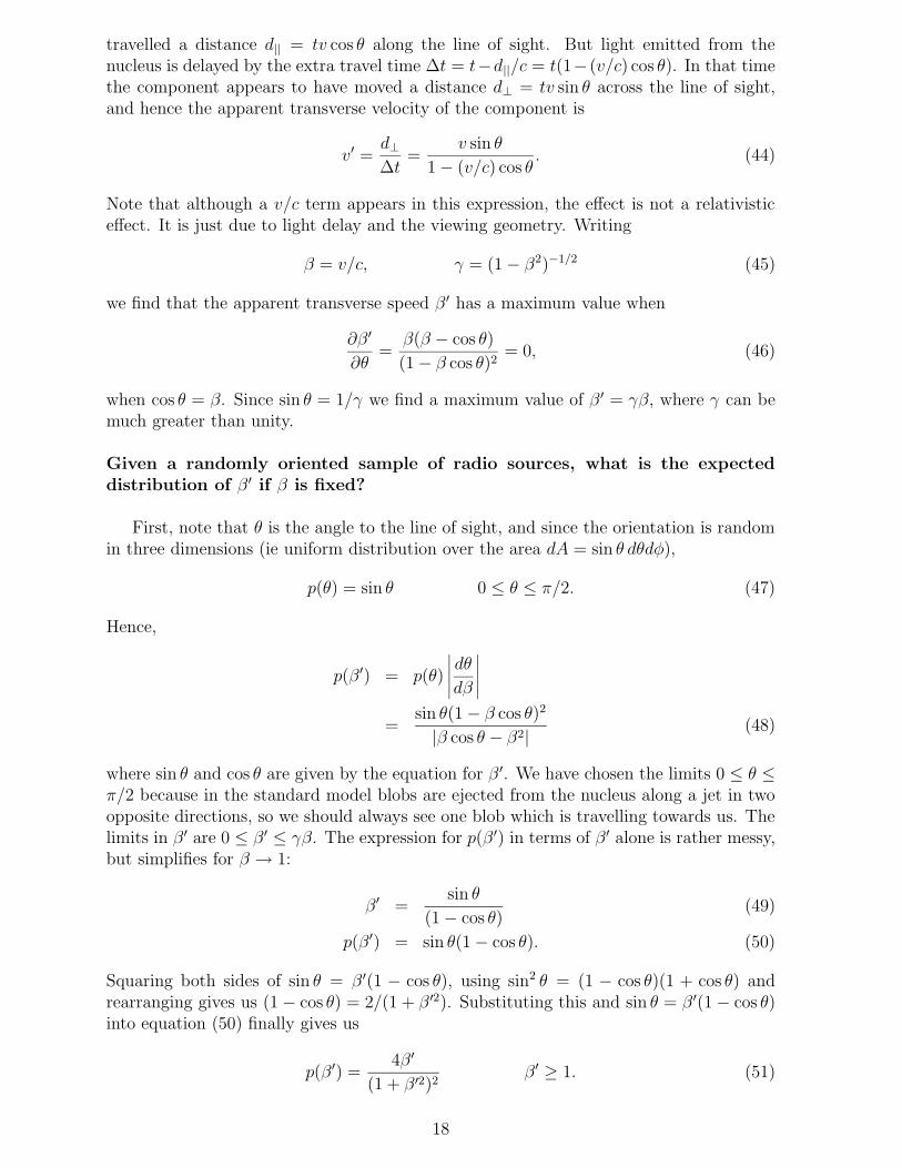
travelled a distance d|| = tv cos θ along the line of sight. But light emitted from thenucleus is delayed by the extra travel time ∆t = t−d||/c = t(1− (v/c) cos θ). In that timethe component appears to have moved a distance d⊥ = tv sin θ across the line of sight,and hence the apparent transverse velocity of the component is

v′ =d⊥

∆t=

v sin θ

1 − (v/c) cos θ. (44)

Note that although a v/c term appears in this expression, the effect is not a relativisticeffect. It is just due to light delay and the viewing geometry. Writing

β = v/c, γ = (1 − β2)−1/2 (45)

we find that the apparent transverse speed β ′ has a maximum value when

∂β′

∂θ=

β(β − cos θ)

(1 − β cos θ)2= 0, (46)

when cos θ = β. Since sin θ = 1/γ we find a maximum value of β ′ = γβ, where γ can bemuch greater than unity.

Given a randomly oriented sample of radio sources, what is the expecteddistribution of β ′ if β is fixed?

First, note that θ is the angle to the line of sight, and since the orientation is randomin three dimensions (ie uniform distribution over the area dA = sin θ dθdφ),

p(θ) = sin θ 0 ≤ θ ≤ π/2. (47)

Hence,

p(β ′) = p(θ)

∣

∣

∣

∣

∣

dθ

dβ

∣

∣

∣

∣

∣

=sin θ(1 − β cos θ)2

|β cos θ − β2| (48)

where sin θ and cos θ are given by the equation for β ′. We have chosen the limits 0 ≤ θ ≤π/2 because in the standard model blobs are ejected from the nucleus along a jet in twoopposite directions, so we should always see one blob which is travelling towards us. Thelimits in β ′ are 0 ≤ β ′ ≤ γβ. The expression for p(β ′) in terms of β ′ alone is rather messy,but simplifies for β → 1:

β′ =sin θ

(1 − cos θ)(49)

p(β ′) = sin θ(1 − cos θ). (50)

Squaring both sides of sin θ = β ′(1 − cos θ), using sin2 θ = (1 − cos θ)(1 + cos θ) andrearranging gives us (1 − cos θ) = 2/(1 + β ′2). Substituting this and sin θ = β ′(1 − cos θ)into equation (50) finally gives us

p(β ′) =4β′

(1 + β ′2)2β′ ≥ 1. (51)

18

The cumulative probability for β ′ is

P (> β ′) =2

(1 + β ′2)β′ ≥ 1. (52)

so the probability of observing a large apparent velocity, say β ′ > 5, is P (β ′ > 5) ≈ 1/13.

In fact, a much larger fraction of powerful radio quasars show superluminal motions,and it now seems likely that the quasars jets cannot be randomly oriented: There mustbe effects operating which tend to favour the selection of quasars jets pointing towardsus, most probably due to an opaque disc shrouding the nucleus.

1.7 The addition of random variables

1.7.1 Multivariate distributions and marginalisation

We can define the joint probability distribution function for two random variables x andy as p(x, y) which is an extension of the single-variable case. Joint distributions for manyrandom variables are known as multivariate distributions.

Univariate distributions for each of x or y can be obtained by integrating, or marginal-ising p(x, y) with respect to the other variable:

p(x) =∫

dy p(x, y)

p(y) =∫

dx p(x, y). (53)

Such a distribution is called the marginal distribution of x.

The variables x and y are independent if their joint distribution function can befactorized,

p(x, y) = p(x)p(y), (54)

for all values of x and y (see Section 3, axiom 4).

1.7.2 The probability distribution of summed random variables

Let us consider the distribution of the sum of two or more random variables: this willlead us on to the Central Limit Theorem which is of critical importance in probabilitytheory and hence astrophysics.

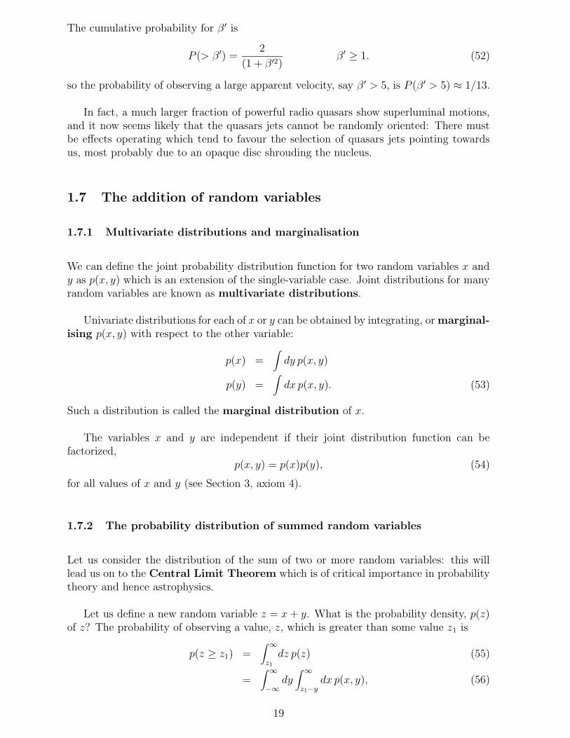
Let us define a new random variable z = x + y. What is the probability density, p(z)of z? The probability of observing a value, z, which is greater than some value z1 is

p(z ≥ z1) =∫ ∞

z1

dz p(z) (55)

=∫ ∞

−∞dy∫ ∞

z1−ydx p(x, y), (56)

19

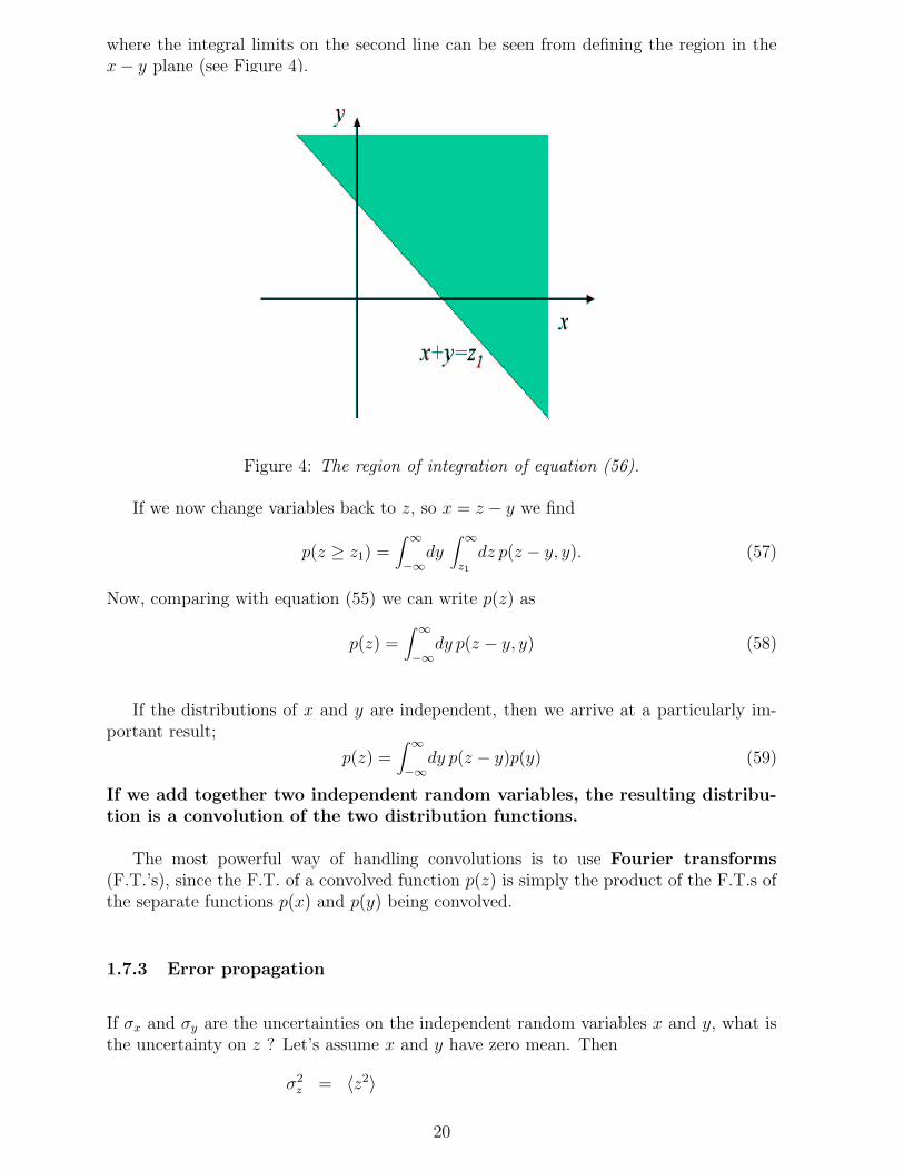
where the integral limits on the second line can be seen from defining the region in thex − y plane (see Figure 4).

Figure 4: The region of integration of equation (56).

If we now change variables back to z, so x = z − y we find

p(z ≥ z1) =∫ ∞

−∞dy

∫ ∞

z1

dz p(z − y, y). (57)

Now, comparing with equation (55) we can write p(z) as

p(z) =∫ ∞

−∞dy p(z − y, y) (58)

If the distributions of x and y are independent, then we arrive at a particularly im-portant result;

p(z) =∫ ∞

−∞dy p(z − y)p(y) (59)

If we add together two independent random variables, the resulting distribu-tion is a convolution of the two distribution functions.

The most powerful way of handling convolutions is to use Fourier transforms(F.T.’s), since the F.T. of a convolved function p(z) is simply the product of the F.T.s ofthe separate functions p(x) and p(y) being convolved.

1.7.3 Error propagation

If σx and σy are the uncertainties on the independent random variables x and y, what isthe uncertainty on z ? Let’s assume x and y have zero mean. Then

σ2z = 〈z2〉

20

=∫ ∞

−∞dzdy z2p(z − y)p(y)

=∫ ∞

−∞dxdy (x + y)2p(x)p(y)

=∫ ∞

−∞dxdy (x2 + 2xy + y2)p(x)p(y)

= 〈x2〉 + 〈y2〉= σ2

x + σ2y (60)

Hence the variance of a sum of independent random variables is equal to the sum of theirvariances. This result is independent of the underlying distribution functions.

In general if z = f(x, y) we can propagate errors by expanding f(x, y) around somearbitrary values, x0 and y0;

f(x, y) = f(x0, y0) + x∂f

∂x+ y

∂f

∂y. (61)

The mean is〈z〉 = f(x0, y0) (62)

and the variance is;

σ2z = 〈z2〉 − 〈z〉2

=∫ ∞

−∞dxdy (f − 〈f〉)2p(x)p(y)

=∫ ∞

−∞dxdy (x2f 2

x + y2f 2y + 2xyfxfy)p(x)p(y) (63)

where we have used the notation fx ≡ ∂f/∂x.

Averaging over the random variables we find

σ2z =

(

∂f

∂x

)2

σ2x +

(

∂f

∂y

)2

σ2y . (64)

This formula will allow us to propagate errors for arbitrary function. Note again that thisis valid for any distribution function, but depends on (1) the underlying variables beingindependent, (2) the function being differentiable and (3) the variation from the meanbeing small enough that the expansion is valid.

1.8 Characteristic functions

Let’s return to the problem of dealing with convolutions of functions. As we noted above,the easiest way to handle convolutions is with Fourier Transforms. In probability theorythe Fourier Transform of a probability distribution function is known as the character-istic function:

φ(k) =∫ ∞

−∞dx p(x)eikx (65)

with reciprocal relation

p(x) =∫ ∞

−∞

dk

2πφ(k)e−ikx (66)

21

(note the choice of where to put the factor 2π is not universal). Hence the characteristicfunction is also the expectation value of eikx;

φ(k) = 〈eikx〉. (67)

Part of the power of characteristic functions is the ease with which one can generateall of the moments of the distribution by differentiation:

mn =

[

d

d(ik)

]n

k=0

φ(k). (68)

This can be seen if one expands φ(k) in a power series;

φ(k) = 1 + ik〈x〉 − 1

2k2〈x2〉 + · · · . (69)

As an example of a characteristic function lets consider the Poisson distribution.

φ(k) =∞∑

n=0

λne−λ

n!eikn = e−λeλeik

. (70)

Hence the characteristic function for the Poisson distribution is

φ(k) = eλ(eik−1). (71)

Returning to the convolution equation (59),

p(z) =∫ ∞

−∞dy p(z − y)p(y), (72)

we shall identify the characteristic function of p(z), p(x), p(y) as φz(k), φx(k) and φy(k)respectively. The characteristic function of p(z) is then

φz(k) =∫ ∞

−∞dz p(z)eikz

=∫ ∞

−∞dz

∫ ∞

−∞dy p(z − y)p(y)eikz

=∫ ∞

−∞dz

∫ ∞

−∞dy (p(z − y)eik(z−y))(p(y)eiky) (73)

Fourier transforming in the last equation we find

φz(k) = φx(k)φy(k), (74)

as expected from the properties of Fourier transforms.

The power of this approach is that the distribution of the sum of a large number ofrandom variables can be easily derived. This result allows us to turn now to the CentralLimit Theorem.

22

1.9 The Central Limit Theorem

The most important, and general, result from probability theory is the Central LimitTheorem. It is

• Central to probability and statistics - without it much of probability and statisticswould be impossible,

• A Limit Theorem because it is only asymptotically true in the case of a largesample.

Finally, it is extremely general, applying to a wide range of phenomena and explains whythe Gaussian distribution appears so often in Nature.

In its most general form, the Central Limit Theorem states that the sum of n randomvalues drawn from a probability distribution function of finite variance, σ2, tends to beGaussian distributed about the expectation value for the sum, with variance nσ2 .

There are two important consequences:

1. The mean of a large number of values tends to be normally distributed regardlessof the probability distribution from which the values were drawn. Hence thesampling distribution is known even when the underlying probabilitydistribution is not. It is for this reason that the Gaussian distribution occupiessuch a central place in statistics. It is particularly important in applications whereunderlying distributions are not known, such as astrophysics.

2. Functions such as the Binomial, Poisson, χ2 or Student-t distribution arise frommultiple drawings of values from some underlying probability distribution, and theyall tend to look like the Gaussian distribution in the limit of large numbers ofdrawings. We saw this earlier when we derived the Gaussian distribution from thePoisson distribution.

The first of these consequences means that under certain conditions we can assumean unknown distribution is Gaussian, if it is generated from a large number ofevents. For a non-astrophysical example, the distribution of human heights is Gaussian,because the total effects of genetics and environment can be thought of as a sum ofinfluences (random variables) that lead to a given height. The height of surface of thesea has a Gaussian distribution, as it is perturbed by the sum of random winds. Thesurface of planets has a Gaussian distribution due to the sum of all the factors that haveformed them. The second consequence means that many distributions, under the rightcircumstances, can be approximated by a Gaussian. This is very useful since theGaussian has many simple properties which we shall use later.

1.9.1 Derivation of the central limit theorem

Let

X =1√n

(x1 + x2 + · · · + xn) (75)

23

be the sum of n random variables xi, each drawn from the same arbitrary underlyingdistribution function, (in general the underlying distributions can be different for each xi,but for simplicity we shall only consider only one). The distribution of X’s generated bythis summation, let’s call it p(X), will be a convolution of the underlying distributions.

From the properties of characteristic functions we know that a convolution of distribu-tion functions is a multiplication of characteristic functions. If the characteristic functionof p(x) is

φx(k) =∫ ∞

−∞dx p(x)eikx = 1 + i〈x〉k − 1

2〈x2〉k2 + O(k3), (76)

where in the last term we have expanded out eikx. Since the sum is over xi/√

n, ratherthan xi we scale all the moments 〈xp〉 → 〈(x/

√n)p〉. From equation (76),we see this is

the same as scaling k → k/√

n. Hence the characteristic function of X is

ΦX(k) = [φx(k/√

n)]n (77)

If we assume that m1 = 〈x〉 = 0, so that m2 = 〈x2〉 = σ2x (this doesn’t affect our results)

then

ΦX(k) =

[

1 − σ2xk

2

2n

]n

→ e−σ2xk2/2 (78)

as n → ∞. Note the higher terms contribute as n−3/2 in the expansion of ΦX(k) and sovanish in the limit. We know that the F.T. of a Gaussian is another Gaussian, but let’sshow that (by ”completing the square”):

p(X) =1

2π

∫ ∞

−∞dk ΦX(k)e−ikX

=e−X2/(2σ2

x)

2π

∫ ∞

−∞dk e(−σ2

xk2+X2/σ2x−2ikX)/2

=e−X2/(2σ2

x)

2π

∫ ∞

−∞dk e(X/σx−ikσx)2/2

=e−X2/(2σ2

x)

√2πσx

. (79)

Thus the sum of random variables, sampled from the same underlying distri-bution, will tend towards a Gaussian distribution, independently of the initialdistribution.

1.9.2 Measurement theory

As a corollary, by comparing equation (75) with the expression for estimating the meanfrom a sample of n variables,

x =1

n

n∑

i=1

xi, (80)

we see that the estimated mean from a sample has a Gaussian distribution with meanm1 = 〈x〉 and variance σ2 = µ2/n as n → ∞.

This has two important consequences.

24

1. This means that if we estimate the mean from a sample, we will always tend towardsthe true mean,

2. The uncertainty in our estimate of the mean will vanish as the sample gets bigger.

This is a remarkable result: for sufficiently large numbers of drawings from an unknowndistribution function with mean 〈x〉 and standard deviation σ/

√n, we are assured by the

Central Limit Theorem that we will get the measurement we want to higher and higheraccuracy, and that the estimated mean of the sampled numbers will have a Gaussiandistribution almost regardless of the form of the unknown distribution. The only conditionunder which this will not occur is if the unknown distribution does not have a finitevariance. Hence we see that all our assumptions about measurement rely onthe Central Limit Theorem.

1.9.3 How the Central Limit Theorem works

We have seen from the above derivation that the Central Limit Theorem arises because inmaking many measurements and averaging them together, we are convolving a probabilitydistribution with itself many times.

We have shown that this has the remarkable mathematical property that in the limitof large numbers of such convolutions, the result always tends to look Gaussian. In thissense, the Gaussian, or normal, distribution is the “smoothest” distribution which can beproduced by natural processes.

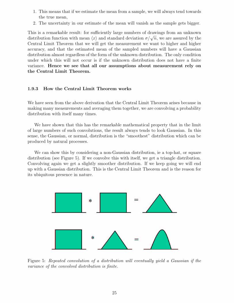
We can show this by considering a non-Gaussian distribution, ie a top-hat, or squaredistribution (see Figure 5). If we convolve this with itself, we get a triangle distribution.Convolving again we get a slightly smoother distribution. If we keep going we will endup with a Gaussian distribution. This is the Central Limit Theorem and is the reason forits ubiquitous presence in nature.

Figure 5: Repeated convolution of a distribution will eventually yield a Gaussian if thevariance of the convolved distribution is finite.

25

1.10 Sampling distributions

Above we showed how the Central Limit Theorem lies at the root of our expectationthat more measurements will lead to better results. Our estimate of the mean of nvariables is unbiased (ie gives the right answer) and the uncertainty on the estimatedmean decreases as σx/

√n, and the distribution of the estimated, or sampled, mean has a

Gaussian distribution. The distribution of the mean determined in this way is known asthe “sampling distribution of the mean”.

How fast the Central Limit Theorem works (i.e. how small n can be before the dis-tribution is no longer Gaussian) depends on the underlying distribution. At one extremewe can consider the case of when the underlying variables are all Gaussian distributed.Then the sampling distribution of the mean will always be a Gaussian, even if n → 1.

But, beware! For some distributions the Central Limit Theorem does not hold. Forexample the means of values drawn from a Cauchy (or Lorentz) distribution,

p(x) =1

π(1 + x2)(81)

never approach normality. This is because this distribution has infinite variance (try andcalculate it and see). In fact they are distributed like the Cauchy distribution. Is this arare, but pathological example ? Unfortunately not. For example the Cauchy distributionappears in spectral line fitting, where it is called the Voigt distribution. Another exampleis if we take the ratio of two Gaussian variables. The resulting distribution has a Cauchydistribution. Hence, we should beware, that although the Central Limit Theorem andGaussian distribution considerably simplify probability and statistics, exceptions do occur,and one should always be wary of them.

1.10.1 The sample variance

The mean of the sample is an estimate of the mean of the underlying distribution. Givenwe may not directly know the variance of the summed variables, σ2

x, is there a similarestimate of the variance of X? This is particularly important in situations where we needto assess the significance of a result in terms of how far away it is from the expected value,but where we only have a finite sample size from which to measure the variance of thedistribution.

We would expect a good estimate of the population variance would be something like

S2 =1

n

n∑

i=1

(xi − 〈x〉)2, (82)

where

〈x〉 =1

n

n∑

i=1

xi (83)

is the sample mean of n values. Let us find the expected value of this sum. First we

26

re-arrange the summation

S2 =1

n

n∑

i=1

(xi − 〈x〉)2 =1

n

∑

x2i −

2

n

∑

i

∑

k

xixk +1

n2

∑

i

∑

k

xixj =1

n

∑

x2i −

(

1

n

n∑

i=1

xi

)2

(84)which is the same result we found in Section 1.4 – the variance is just the mean of thesquare minus the square of the mean. If all the xi are drawn independently then

〈∑

i

f(xi)〉 =∑

i

〈f(xi)〉 (85)

where f(x) is some arbitrary function of x. If i = j then

〈xixj〉 = 〈x2〉 i = j, (86)

and when i and j are different

〈xixj〉 = 〈x〉2 i 6= j. (87)

The expectation value of our estimator is then

〈S2〉 =

⟨

1

n

∑

x2i −

(

1

n

n∑

i=1

xi

)2⟩

=1

n

∑

〈x2〉 − 1

n2

∑

i

∑

j 6=i

〈x〉2 − 1

n2

∑

〈x2〉

= 〈x2〉 − n(n − 1)

n2〈x〉2 − n

n2〈x2〉

=(

1 − 1

n

)

〈x2〉 − n(n − 1)

n2〈x〉2

=(n − 1)

n(〈x2〉 − 〈x〉2). (88)

The variance is defined as σ2 = 〈x2〉 − 〈x〉2, so S2 will underestimate the variance by thefactor (n − 1)/n. This is because an extra variance term, σ2/n, has appeared due to theextra variance in our estimate in the mean. Since the square of the mean is subtractedfrom the mean of the square, this extra variance is subtracted off from our estimate of thevariance, causing the underestimation. To correct for this we should change our estimateto

S2 =1

n − 1

n∑

i=1

(xi − 〈x〉)2 (89)

which is an unbiased estimate of σ2, independent of the underlying distribution. It isunbiased because its expectation value is always σ2 for any n when the mean is estimatedfrom the sample.

Note that if the mean is know, and not estimated from the sample, this extra variancedoes not appear, in which case equation (82) is an unbiased estimate of the samplevariance.

27

1.10.2 Measuring quasar variation

We want to look for variable quasars. We have two CCD images of one field taken sometime apart and we want to pick out the quasars which have varied significantly more thanthe measurement error which is unknown.

In this case

S2 =1

n − 1

n∑

i=1

(∆mi − ∆m)2 (90)

is the unbiased estimate of the variance of ∆m. We want to keep ∆m 6= 0 (i.e. we want tomeasure ∆m from the data) to allow for possible calibration errors. If we were confidentthat the calibration is correct we can set ∆m = 0, and we could return to the definition

σ2 =1

n

∑

i

(∆m)2. (91)

Suppose we find that one of the ∆m, say ∆mi, is very large, can we assess the signif-icance of this result? One way to estimate its significance is from

t =∆mi − ∆m

S. (92)

If the mean is know this is distributed as a standardised Gaussian (ie t has unit variance)if the measurement errors are Gaussian.

But if we can only estimate the mean from the data, t is distributed as Student-t9.The Student-t distribution looks qualitatively similar to a Gaussian distribution, but ithas larger tails, due to the variations in the measured mean and variance.

9The name ‘Student’ comes about because the first derivation was part of an undergraduate exam.

28

PART TWO

2 STATISTICAL INFERENCE

2.1 Model fitting and parameter estimation

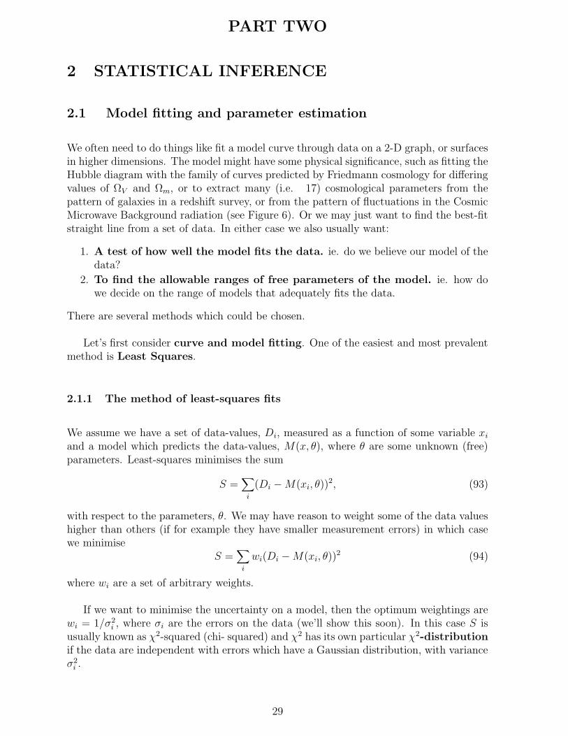
We often need to do things like fit a model curve through data on a 2-D graph, or surfacesin higher dimensions. The model might have some physical significance, such as fitting theHubble diagram with the family of curves predicted by Friedmann cosmology for differingvalues of ΩV and Ωm, or to extract many (i.e. 17) cosmological parameters from thepattern of galaxies in a redshift survey, or from the pattern of fluctuations in the CosmicMicrowave Background radiation (see Figure 6). Or we may just want to find the best-fitstraight line from a set of data. In either case we also usually want:

1. A test of how well the model fits the data. ie. do we believe our model of thedata?

2. To find the allowable ranges of free parameters of the model. ie. how dowe decide on the range of models that adequately fits the data.

There are several methods which could be chosen.

Let’s first consider curve and model fitting. One of the easiest and most prevalentmethod is Least Squares.

2.1.1 The method of least-squares fits

We assume we have a set of data-values, Di, measured as a function of some variable xi

and a model which predicts the data-values, M(x, θ), where θ are some unknown (free)parameters. Least-squares minimises the sum

S =∑

i

(Di − M(xi, θ))2, (93)

with respect to the parameters, θ. We may have reason to weight some of the data valueshigher than others (if for example they have smaller measurement errors) in which casewe minimise

S =∑

i

wi(Di − M(xi, θ))2 (94)

where wi are a set of arbitrary weights.

If we want to minimise the uncertainty on a model, then the optimum weightings arewi = 1/σ2

i , where σi are the errors on the data (we’ll show this soon). In this case S isusually known as χ2-squared (chi- squared) and χ2 has its own particular χ2-distributionif the data are independent with errors which have a Gaussian distribution, with varianceσ2

i .

29

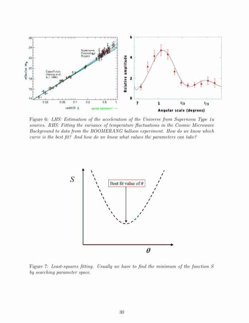
Figure 6: LHS: Estimation of the acceleration of the Universe from Supernova Type 1asources. RHS: Fitting the variance of temperature fluctuations in the Cosmic MicrowaveBackground to data from the BOOMERANG balloon experiment. How do we know whichcurve is the best fit? And how do we know what values the parameters can take?

Figure 7: Least-squares fitting. Usually we have to find the minimum of the function Sby searching parameter space.

30

In general it is not possible to find the best-fitting θ values in one single step: we haveto evaluate S for a range of values of θ and choose the values of θ which give the smallestvalue of S. Hence the name Least Squares.

2.1.2 Estimating a mean from Least Squares

What is the optimal (ie smallest error) estimate of the mean, 〈x〉, of a set of observations,xi, and what is its variance? In this case we want to minimise the function

S =∑

i

wi(xi − 〈x〉)2, (95)

with respect to 〈x〉. Hence

∂S

∂〈x〉 = 2∑

i

wi(xi − 〈x〉) = 0, (96)

which has the solution

〈x〉 =

∑

i wixi∑

i wi

. (97)

The variance on this can be found by Propagation of Errors (see Section 1.7.3):

σ2(〈x〉) =∑

i

(

∂〈x〉∂xi

)2

σ2i

=

∑

i w2i σ

2i

(∑

j wj)2(98)

We can use this to find the set of weights which will minimise the error on the mean, byminimising σ2(〈x〉) with respect to the wi:

∂σ2(〈x〉)∂wi

= −2∑

i w2i σ

2i

(∑

j wj)3+

2wiσ2i

(∑

j wj)2(99)

which implies∑

i

w2i σ

2i = wiσ

2i

∑

j

wj. (100)

This last equation is solved when

wi =1

σ2i

. (101)

This set of weights is the minimum variance weighting scheme.

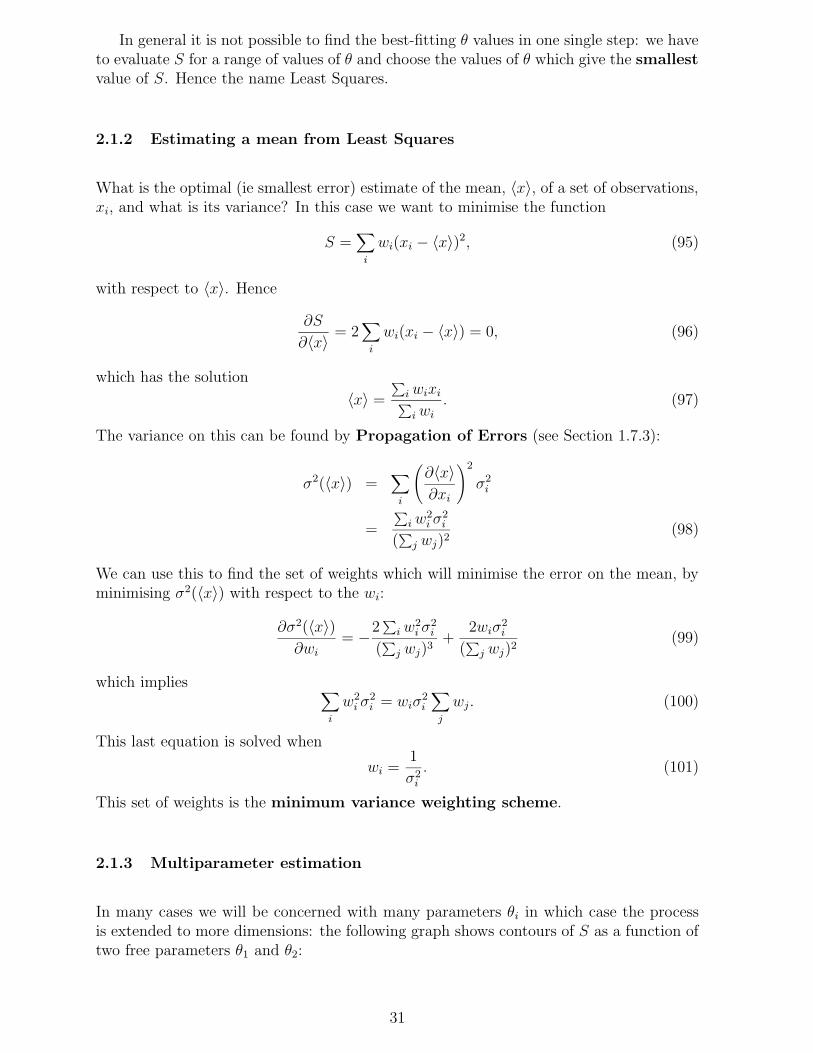
2.1.3 Multiparameter estimation

In many cases we will be concerned with many parameters θi in which case the processis extended to more dimensions: the following graph shows contours of S as a function oftwo free parameters θ1 and θ2:

31

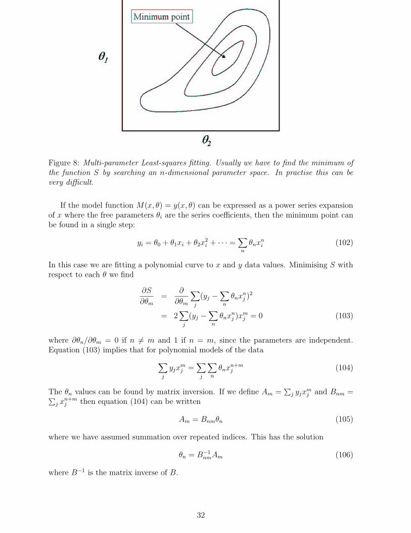
Figure 8: Multi-parameter Least-squares fitting. Usually we have to find the minimum ofthe function S by searching an n-dimensional parameter space. In practise this can bevery difficult.

If the model function M(x, θ) = y(x, θ) can be expressed as a power series expansionof x where the free parameters θi are the series coefficients, then the minimum point canbe found in a single step:

yi = θ0 + θ1xi + θ2x2i + · · · =

∑

n

θnxni (102)

In this case we are fitting a polynomial curve to x and y data values. Minimising S withrespect to each θ we find

∂S

∂θm

=∂

∂θm

∑

j

(yj −∑

n

θnxnj )2

= 2∑

j

(yj −∑

n

θnxnj )xm

j = 0 (103)

where ∂θn/∂θm = 0 if n 6= m and 1 if n = m, since the parameters are independent.Equation (103) implies that for polynomial models of the data

∑

j

yjxmj =

∑

j

∑

n

θnxn+mj (104)

The θn values can be found by matrix inversion. If we define Am =∑

j yjxmj and Bnm =

∑

j xn+mj then equation (104) can be written

Am = Bnmθn (105)

where we have assumed summation over repeated indices. This has the solution

θn = B−1nmAm (106)

where B−1 is the matrix inverse of B.

32

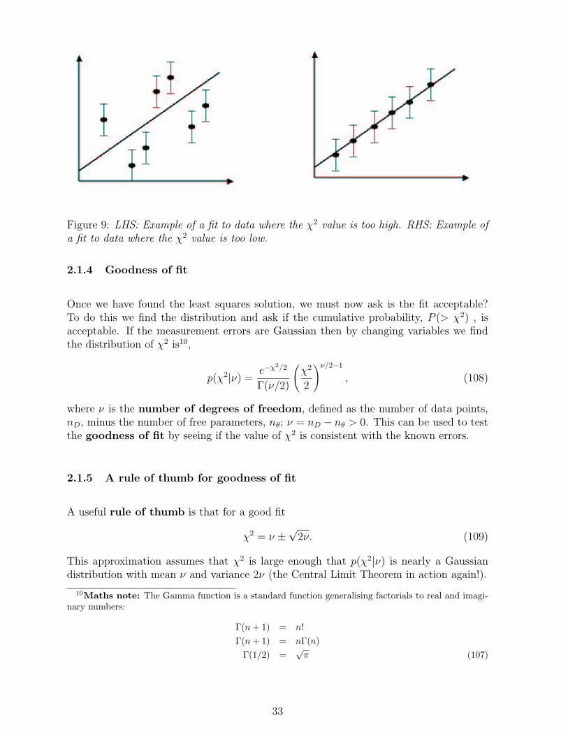
Figure 9: LHS: Example of a fit to data where the χ2 value is too high. RHS: Example ofa fit to data where the χ2 value is too low.

2.1.4 Goodness of fit

Once we have found the least squares solution, we must now ask is the fit acceptable?To do this we find the distribution and ask if the cumulative probability, P (> χ2) , isacceptable. If the measurement errors are Gaussian then by changing variables we findthe distribution of χ2 is10,

p(χ2|ν) =e−χ2/2

Γ(ν/2)

(

χ2

2

)ν/2−1

, (108)

where ν is the number of degrees of freedom, defined as the number of data points,nD, minus the number of free parameters, nθ; ν = nD − nθ > 0. This can be used to testthe goodness of fit by seeing if the value of χ2 is consistent with the known errors.

2.1.5 A rule of thumb for goodness of fit

A useful rule of thumb is that for a good fit

χ2 = ν ±√

2ν. (109)

This approximation assumes that χ2 is large enough that p(χ2|ν) is nearly a Gaussiandistribution with mean ν and variance 2ν (the Central Limit Theorem in action again!).

10Maths note: The Gamma function is a standard function generalising factorials to real and imagi-

nary numbers:

Γ(n + 1) = n!

Γ(n + 1) = nΓ(n)

Γ(1/2) =√

π (107)

33

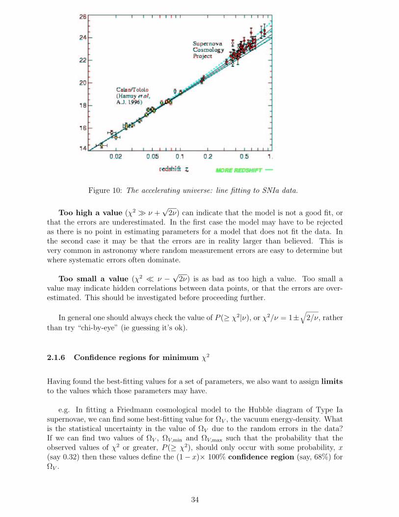
Figure 10: The accelerating universe: line fitting to SNIa data.

Too high a value (χ2 ν +√

2ν) can indicate that the model is not a good fit, orthat the errors are underestimated. In the first case the model may have to be rejectedas there is no point in estimating parameters for a model that does not fit the data. Inthe second case it may be that the errors are in reality larger than believed. This isvery common in astronomy where random measurement errors are easy to determine butwhere systematic errors often dominate.

Too small a value (χ2 ν −√

2ν) is as bad as too high a value. Too small avalue may indicate hidden correlations between data points, or that the errors are over-estimated. This should be investigated before proceeding further.

In general one should always check the value of P (≥ χ2|ν), or χ2/ν = 1±√

2/ν, rather

than try “chi-by-eye” (ie guessing it’s ok).

2.1.6 Confidence regions for minimum χ2

Having found the best-fitting values for a set of parameters, we also want to assign limitsto the values which those parameters may have.

e.g. In fitting a Friedmann cosmological model to the Hubble diagram of Type Iasupernovae, we can find some best-fitting value for ΩV , the vacuum energy-density. Whatis the statistical uncertainty in the value of ΩV due to the random errors in the data?If we can find two values of ΩV , ΩV,min and ΩV,max such that the probability that theobserved values of χ2 or greater, P (≥ χ2), should only occur with some probability, x(say 0.32) then these values define the (1− x)× 100% confidence region (say, 68%) forΩV .

34

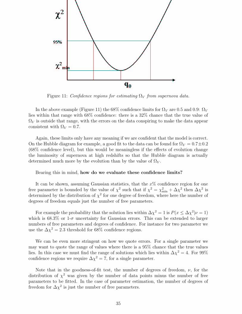
Figure 11: Confidence regions for estimating ΩV from supernova data.

In the above example (Figure 11) the 68% confidence limits for ΩV are 0.5 and 0.9: ΩV

lies within that range with 68% confidence: there is a 32% chance that the true value ofΩV is outside that range, with the errors on the data conspiring to make the data appearconsistent with ΩV = 0.7.

Again, these limits only have any meaning if we are confident that the model is correct.On the Hubble diagram for example, a good fit to the data can be found for ΩV = 0.7±0.2(68% confidence level), but this would be meaningless if the effects of evolution changethe luminosity of supernova at high redshifts so that the Hubble diagram is actuallydetermined much more by the evolution than by the value of ΩV .

Bearing this in mind, how do we evaluate these confidence limits?

It can be shown, assuming Gaussian statistics, that the x% confidence region for onefree parameter is bounded by the value of χ2 such that if χ2 = χ2

min + ∆χ2 then ∆χ2 isdetermined by the distribution of χ2 for one degree of freedom, where here the number ofdegrees of freedom equals just the number of free parameters.

For example the probability that the solution lies within ∆χ2 = 1 is P (x ≤ ∆χ2|ν = 1)which is 68.3% or 1-σ uncertainty for Gaussian errors. This can be extended to largernumbers of free parameters and degrees of confidence. For instance for two parameter weuse the ∆χ2 = 2.3 threshold for 68% confidence regions.

We can be even more stringent on how we quote errors. For a single parameter wemay want to quote the range of values where there is a 95% chance that the true valueslies. In this case we must find the range of solutions which lies within ∆χ2 = 4. For 99%confidence regions we require ∆χ2 = 7, for a single parameter.

Note that in the goodness-of-fit test, the number of degrees of freedom, ν, for thedistribution of χ2 was given by the number of data points minus the number of freeparameters to be fitted. In the case of parameter estimation, the number of degrees offreedom for ∆χ2 is just the number of free parameters.

35

2.2 Maximum Likelihood Methods

Minimum-χ2 is a useful tool for estimating goodness-of-fit and confidence regions onparameters. However it can only be used in the case where we have a set of measureddata values with a known, Gaussian-distributed, scatter about some model values. Amore general tool is to use the technique of Maximum Likelihood.

The “likelihood function” is the joint probability distribution, p(D1, · · · , Dn|θ1, · · · , θm)of n measured data values, Di, drawn from a model distribution with m free parametersθj:

L(D1, · · · , Dn|θ1, · · · , θm) = p(D1, · · · , Dn|θ1, · · · , θm). (110)

If the data values are independent then;

L(D1, · · · , Dn|θ1, · · · , θm) = p(D1|θ1, · · · , θm) · · · p(Dn|θ1, · · · , θm)

=n∏

i=1

p(Di|θ1, · · · , θm). (111)

The technique of maximum likelihood maximises this function with respect to thefree parameters θ. That is, it chooses the values of parameters which most closely simulatethe distribution of the observed data values. In practice, it is easier to maximise ln(L)rather than L: i.e.

∂

∂θln L = 0. (112)

The method is particularly useful when the type of models being investigated are notthose that predict a value for each of a set of measured quantities, but rather those thatpredict the statistical distribution of values in a sample. In this case, one may not knowthe error on any individual measurement. It is also very useful when the distribution ofthe data is known to be non-Gaussian. In this case Maximum Likelihood is both veryversatile and simple to apply.

2.2.1 The flux distribution of radio sources

The distribution of flux densities of extragalactic radio sources are distributed as a power-law with slope −α, say. In a non-evolving Euclidean universe α = 3/2 (can you provethis?) and departure of α from the value 3/2 is evidence for cosmological evolution ofradio sources. This was the most telling argument against the steady-state cosmology inthe early 1960’s (even though they got the value of a wrong by quite a long way).

Given observations of radio sources with flux densities S above a known, fixed mea-surement limit S0, what is the best estimate for α?

The model probability distribution for S is

p(S)dS = (α − 1)Sα−10 S−αdS (113)

36

where the factors α− 1 in front of the term arise from the normalization requirement

∫ ∞

S0

dS p(S) = 1. (114)

So the likelihood function L for n observed sources is

L =n∏

i=1

(α − 1)Sα−10 S−α

i (115)

with logarithm

ln L =n∑

i=1

(ln(α − 1) + (α − 1) ln S0 − α ln Si). (116)

Maximising ln L with respect to α:

∂

∂αln L =

n∑

i=1

(

1

α − 1+ ln S0 − ln Si

)

= 0 (117)

we find the minimum whenα = 1 +

n∑n

i=1 ln Si

S0

. (118)

Suppose we only observe one source with flux twice the cut-off, S1 = 2S0, then

α = 1 +1

ln 2= 2.44 (119)

but with a large uncertainty. Clearly, as Si = S0 we find α → ∞ as expected. In factα = 1.8 for bright radio sources at low frequencies, significantly steeper than 1.5.

2.2.2 Goodness-of-fit and confidence regions from maximum likelihood

In cases where we are fitting a set of data values with known Gaussian errors, thenmaximum-likelihood is precisely equivalent to minimum-χ2, since in this case ln L =−χ2/2. The distribution of −2 ln L is then the χ2-distribution and hence we can readilycalculate a goodness of fit.

In cases such as the example in Section 2.2.1, however, the probability distributionassumed for the model is not Gaussian – it is the power-law model for the source counts.In this case we do not know what the expected distribution for the ln(likelihood) actuallyis, and hence we cannot estimate a goodness-of-fit.

In the limit of large numbers of observations, we can still estimate confidence regionsfor parameters, however (another example of the operation of the Central Limit Theo-rem) in that we expect the distribution of −1/2 ln L to have the χ2 distribution with thenumber of degrees of freedom equal to the number of free parameters (c.f. the estimationof confidence regions in the case of minimum χ2).

In practice one would instead plot out the likelihood surface in parameter space. Inthe case of two parameter this will generally be an ellipse.

37

2.2.3 Estimating parameter uncertainty

Although plotting out the likelihood contours around the maximum is a good indicatorof the parameter uncertainty, it can sometimes be computationally expensive, especiallyfor large data sets, and many parameters. An alternative is to use the second derivativeof the log-likelihood:

σ2(θi) = −(

∂2 ln L

∂θ2

)−1

(120)

to estimate the error. The idea is that the surface of the likelihood function can beapproximated about its maximum, at θmax, by a Gaussian;

L(θ) =e−∆θ2/(2σ2(θ))

√2πσ(θ)

(121)

where ∆θ = θ − θmax. Equation (120) can be verified by expand ln L to 2nd order in∆θ and differentiating. This can be generalized to multiple parameters by the covariancematrix

〈∆θi∆θj〉 = F−1ij (122)

where

Fij = −∂2 ln L

∂θi∂θj

(123)

is called the Fisher Information Matrix, after the Statistician R.A. Fisher. This canbe used to estimate both the conditional errors, σ2

cond(θ) = 1/Fii, where we assume theother parameters are known, and the marginalised errors, [F−1]ii. These two quantitiessatisfy the relation

1/Fii ≤ [F−1]ii. (124)

The Fisher Matrix is commonly used in cosmology in both survey design and analysis.

2.3 Hypothesis testing

2.3.1 Introduction

The concept of testing goodness-of-fit of a model, and of estimating confidence regionsfor parameters, is part of the more general philosophical problem of hypothesis testing:

Given a set of data, can we distinguish between two (or more) hypothesesor models which predict those data values?

In some sense, we wish to compare the goodness of fit of the two hypotheses. Theretend to be two schools of thought among statisticians, the Frequentists and Bayesians wemet at the beginning, over how to do this, and the subject is very controversial. Theproblem arises from Bayes’ Theorem, published posthumously in 1763, which describeshow to new information changes a probability distribution. It was really the first attemptto use statistical axioms to make decisions on hypotheses. If we follow the logical con-sequences of Bayes’ work, we find that the tests of goodness-of-fit of models describedabove are fundamentally incomplete in their treatment of the problem.

38

2.3.2 Bayes Theorem

Suppose we are given some information about a physical experiment, which we shalldenote by I. We carry out the experiment and get a result, or set of data, denoted D.Now we want to choose between two hypotheses H1 and H2. From the axioms we metin Lecture 1, we can say that the conditional joint probability of obtaining the result Dand of Hi being correct, given our prior information I, is

p(HiD|I) = p(D|I)p(Hi|DI). (125)

That is, the joint probability of the hypothesis and data (result) being true, given theinitial information, p(H1D|I), is the probability of obtaining that data set given only theinitial information, p(D|I), multiplied by the probability of Hi being correct given theprior information I and data D, p(Hi|DI) (this is known as the a posteriori probabil-ity). This is not very useful, but if we swap Hi and D we find

p(HiD|I) = p(Hi|I)p(D|HiI), (126)

which now says that this joint probability is the likelihood, p(D|HiI) (the probability ofgetting a data set, D, from hypothesis Hi given I), multiplied by the prior probability,p(Hi|I), of the hypothesis Hi being true in the absence of any data other than I. Thus

p(Hi|DI) =p(Hi|I)p(D|HiI)

p(D|I). (127)

This is Bayes’ Theorem. If we want to choose between the two hypotheses H1 andH2, we should evaluate p(H1|DI) and p(H2|DI) and choose the most probable result.The factor, p(D|I), called the evidence, is the same for H1 and H2, so we can use thelikelihood ratio,

p(H1|DI)

p(H2|DI)=

p(H1|I)p(D|H1I)

p(H2|I)p(D|H2I)(128)

to choose the higher probability.

If we assume that the two prior probabilities are equal, then we just choose the hy-pothesis with the highest likelihood. In fact, it is common to ignore Bayes’ Theorementirely and simply determine the likelihoods, and proponents of such tests do not con-sider the possible non-equality of the prior probabilities. Indeed, Bayes postulated that inthe absence of any information to the contrary we should assume equal prior probabilities(Bernoulli’s “Principle of Insufficient Reason”).

2.3.3 Updating the probability of a hypothesis

If we now obtain some more information, perhaps from a new experiment, then we can useBayes’ theorem to update our estimate of the probabilities associated with each hypothe-sis. The problem reduces to that of showing that adding the results of a new experimentto the probability of a hypothesis is the same as doing the two experiments first, and thenseeing how they both effect the probability of the hypothesis. In other words it shouldnot matter how we gain our information, the effect on the probability of the hypothesisshould be the same.

39

We start with Bayes’ expression for the posteriori probability of a hypothesis,

p(H|DI) =p(H|I)p(D|HI)

p(D|I). (129)

Let say we do a new experiment with new data, D′. We can then express this by trans-forming equation (129) by D → D′ and letting the old data become part of the priorinformation I → DI. Bayes’ theorem is now

p(H|D′DI) =p(H|DI)p(D′|HDI)

p(D′|DI). (130)

We now notice that the new prior in this expression is just the old posteriori probabilityfrom equation (129), and that the new likelihood is just

p(D′|DHI) =p(D′D|HI)

p(D|HI). (131)

Substituting in the old posteriori probability and this expression for the new likelihoodwe find

p(H|D′DI) =p(H|I)p(D′D|HI)

p(D′D|I)(132)

which has the same form as equation (129), the outcome from the initial experiment, butnow with the new data incorporated, ie. we have shown D → D′ and I → DI is thesame is D → D′D. This shows us that it doesn’t matter how we add in new information.Bayes’ theorem gives us a natural way of improving our statistical inferencesas our state of knowledge increases.

2.3.4 The prior distribution

In Lecture 1 we discussed that Frequentists and Bayesians have different definitions ofprobability, which can lead to different results. These discrepancies occur particularlyin parameter estimation: a Bayesian would multiply the likelihood function for a givenparameter value by a prior probability. The maximum likelihood estimate of α in Section2.2.1 is Bayesian if the prior probability is assumed to be a constant per unit α.

But the Bayesian estimate will change if we assume a different prior, such as constantprobability per unit ln α. We may do this if α has to be positive, or if we want to searchfor the most likely α over many orders of magnitude. In this case

p(ln α) =1

αp(α). (133)

Here our initial problem of how we assign probabilities becomes most apparent. It is thisarbitrariness that is unattractive to Frequentists, who ignore the prior. The Bayesianpoint of view is that the prior exists and so we must choose something.

But it is as well to be aware that ignoring priors is equivalent to making a specificchoice of prior by default. Hypothesis testing and parameter estimation is a minefield ofphilosophical uncertainty! Some astronomers use both Bayesian and Frequentist methods

40

to satisfy both. Another view is that if the choice of prior really matters, there cannot beenough information in the data to decide which is the most likely hypothesis.

In the next section we look at one application where Bayesian methods have becomewidely accepted.

2.4 Imaging process and Bayes’ Theorem

2.4.1 Using the prior

A common problem in image processing is to correct an image for the two main processeswhich degrade its appearance and hence our interpretation of the scene which it captures.These two processes are the convolution (or smoothing, or blurring) of an image by someinstrumental response, and the addition of noise to the image (which depending on theapplication may arise before the blurring process, as in radioastronomy interferometerimages, or after the blurring process, as in images from optical telescopes).

Even if we knew precisely the blurring function of the system and its noise properties,there are two reasons why we cannot precisely reconstruct what the scene should look likeif viewed in the absence of these factors.

• First, it may not be possible to unambiguously deconvolve the blurring. Rememberthat convolution by a function is equivalent in Fourier space to multiplying thescene’s Fourier transform by the Fourier transform of the blurring function. Hencedeconvolution is the process of dividing the transform of the observed image by thetransform of the blurring function. In general that process will not be defined at allspatial frequencies, and some spatial frequencies in the result will have undefinedvalues. Even in regions where the division is defined, the addition of noise to thesystem is likely to have an unstable effect in the deconvolving process.

• Second, the noise is a random statistical process, and so we cannot unambiguouslycalculate the intensity at a particular point in a scene, given the observed image:we can only calculate probabilities that the scene has any particular value at eachpoint.

So image reconstruction can be seen to be a process of statistical inference, in whichwe have to estimate the most likely (in some sense not yet defined) values for the scenegiven what we know about the problem: we want to find the best-fitting model scene.Now in this case, straightforward application of the maximum likelihood technique tochoose the best-fitting model will not work: we have n pixels of data, but each of thosehas to be a free parameter in the model. If we want to make progress we need to addin some extra information, and Bayes’ theorem gives us a way of doing that. We shouldchoose the model scene which maximises

p(scene|initial information)p(image data|scene, initial information). (134)

The second term is the likelihood, but we now have the ability to bring additional infor-mation to the problem by means of the prior.

41

What can we say about the scene before we attempt to measure an image of it? Re-member that one of the problems in the deconvolution is that at some spatial frequenciesthe Fourier transform may be undefined. Equivalently, the final deconvolved image couldhave sinusoidal waves of arbitrary amplitude imposed upon it, unless we take steps tosuppress them. Similarly, the presence of noise would allow large fluctuations to exist athigh spatial frequencies in the image, which in reality would not be appropriate. So oneway to carry out the scene reconstruction is to enforce a prior which penalises solutionswhich are not smooth.

A number of schemes exist to do this: perhaps the most publicised is the MaximumEntropy prior.

2.4.2 Maximum Entropy

Imagine constructing a scene by randomly putting N photons into m pixels. In each pixelthere will be ni = Npi photons. The number of ways in which we can randomly place Nidentical photons in m pixels is

N !

n1!n2! · · ·nm!→ exp

(

−∑

i

ni ln(

ni

N

)

)

(135)

where the right hand side limit can be derived by taking the natural log and using Stirling’sformula;

ln N ! −∑

i

ln ni! → −N + N ln N −∑

i

(−ni + ni ln ni)

= −N +∑

i

ni ln N + N −∑

i

ni ln ni

= −∑

i

ni ln(

ni

N

)

. (136)

We have assumed each photon is indistinguishable. The quantity in the outer bracketsin equation (135), is known as the image entropy, H, by analogy with the entropyof statistical mechanics, which can also be deduced by considering the multiplicity ofmicrostates. A prior probability can thus be assigned for each scene which is just propor-tional to exp[H]. This is the usefulness of Max-Ent, that it gives us a way of choosingthe prior in the case of image processing.

For large N this prior is equal to the number of ways the scene could have beenrandomly generated. In this “random scene” model the prior is a maximum whenevery pixel has an equal number of photons: the “simplest” scene, the one which adds inthe least amount of structure consistent with the observed data, is preferred over morecomplicated scenes. One feature of this choice of prior is that the reconstructed scenemust be positive: you can’t have a scene with negative numbers of photons. For manyimages this is a good property to embody into the prior, but this may not be appropriatefor other types of image where negative values may be allowed.

In practice, we may have more information about the scene than assumed above, inwhich case we can incorporate that information also into the maximum entropy prior.

42

Maximum entropy does not force us to favour only a completely uniform intensity distri-bution.

Maximum entropy has found favour largely because it works, but there are clearlyother choices of prior which could be made. Note that the maximum entropy prior doesnot contain any information about the intensity of pixels relative to their neighbours,such as you might require if you wanted to adopt the smoothest solution to the scenerestoration. If the pixels in the scene were randomly permuted in position, the imageentropy would be unaffected. This suggests that, for images with complex structure, achoice of prior which did incorporate information about pixel inter-relationships mightbe more effective.

The idea of Maximum Entropy has been extended by E. Jaynes, who has suggestedthat it is a way of subjectively solving the problem of how to choose a prior in anysituation, and has further elaborated on the connection with statistical physics . However,to maintain rigour in this approach, the methods can be rather complex. Again usingthis approach become a matter of personal choice.

2.5 Non-parametric statistics

A non-parametric statistical test is one in which the outcome does not depend onthe probability distribution which generated the data. Some statisticians prefer tocall such tests “distribution-free”. By implication, it is not necessary to know that theprobability distribution that generated the data values (and their errors) was in order toapply a non-parametric test. This is a vital property in many areas (from psychology toastronomy) where the distributions are not known. The tests are usually quick and easyto apply – another practical advantage.

If the underlying distribution is known then a parametric test may be more powerful,but usually this advantage is small and is more than offset by the advantage of the non-parametric tests. Non-parametric tests are also often valid for very small samples.

There are three important tests which I shall deal with here,

1. The χ2 Goodness-of-Fit Test.

2. The Kolmogorov-Smirnov Test

3. The Spearman Rank Correlation Coefficient.

2.5.1 The χ2-goodness-of-fit test

We have already met the parametric χ2 goodness-of-fit test, in which data values xi

are compared with model predictions. If the errors on the data values are Gaussiandistributed, then the quantity

χ2 =n∑

i=1

(xi − λi)2

σ2i

(137)

43

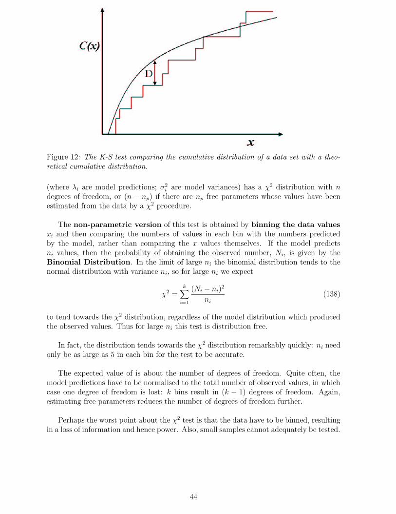
Figure 12: The K-S test comparing the cumulative distribution of a data set with a theo-retical cumulative distribution.

(where λi are model predictions; σ2i are model variances) has a χ2 distribution with n

degrees of freedom, or (n − np) if there are np free parameters whose values have beenestimated from the data by a χ2 procedure.

The non-parametric version of this test is obtained by binning the data valuesxi and then comparing the numbers of values in each bin with the numbers predictedby the model, rather than comparing the x values themselves. If the model predictsni values, then the probability of obtaining the observed number, Ni, is given by theBinomial Distribution. In the limit of large ni the binomial distribution tends to thenormal distribution with variance ni, so for large ni we expect

χ2 =k∑

i=1

(Ni − ni)2

ni

(138)

to tend towards the χ2 distribution, regardless of the model distribution which producedthe observed values. Thus for large ni this test is distribution free.

In fact, the distribution tends towards the χ2 distribution remarkably quickly: ni needonly be as large as 5 in each bin for the test to be accurate.

The expected value of is about the number of degrees of freedom. Quite often, themodel predictions have to be normalised to the total number of observed values, in whichcase one degree of freedom is lost: k bins result in (k − 1) degrees of freedom. Again,estimating free parameters reduces the number of degrees of freedom further.

Perhaps the worst point about the χ2 test is that the data have to be binned, resultingin a loss of information and hence power. Also, small samples cannot adequately be tested.

44

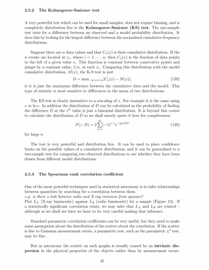
2.5.2 The Kolmogorov-Smirnov test

A very powerful test which can be used for small samples, does not require binning, and iscompletely distribution free is the Kolmogorov-Smirnov (KS) test. The one-sampletest tests for a difference between an observed and a model probability distribution. Itdoes this by looking for the largest difference between the normalised cumulative frequencydistributions.

Suppose there are n data values and that Cn(x) is their cumulative distribution. If then events are located at xi, where i = 1, · · · , n, then Cn(x) is the fraction of data pointsto the left of a given value x. This function is constant between consecutive points andjumps by a constant value, 1/n, at each xi. Comparing this distribution with the modelcumulative distribution, M(x), the K-S test is just

D = max−∞<x<∞|Cn(x) − M(x)|, (139)

ie it is just the maximum difference between the cumulative data and the model. Thistype of statistic is most sensitive to differences in the mean of two distributions.

The KS test is clearly insensitive to a rescaling of x. For example it is the same usingx or ln x. In addition the distribution of D can be calculated as the probability of findingthe difference D at the ith value is just a binomial distribution. It is beyond this courseto calculate the distribution of D so we shall merely quote it here for completeness:

P (> D) = 2∞∑

i=1

(−1)i−1e−2ni2D2

(140)

for large n.

The test is very powerful and distribution free. It can be used to place confidencelimits on the possible values of a cumulative distribution, and it can be generalised to atwo-sample test for comparing two observed distributions to see whether they have beendrawn from different model distributions.

2.5.3 The Spearman rank correlation coefficient

One of the most powerful techniques used in statistical astronomy is to infer relationshipsbetween quantities by searching for a correlation between theme.g. is there a link between radio and X-ray emission from quasars?Plot LX (X-ray luminosity) against LR (radio luminosity) for a sample (Figure 13). Ifa statistically significant correlation exists, we may infer that LX and LR are related –although as we shall see later we have to be very careful making that inference.

Standard parametric correlation coefficients can be very useful, but they need to makesome assumption about the distribution of the scatter about the correlation. If the scatteris due to Gaussian measurement errors, a parametric test, such as the parametric χ2 test,may be fine.

But in astronomy the scatter on such graphs is usually caused by an intrinsic dis-persion in the physical properties of the objects rather than by measurement errors.

45

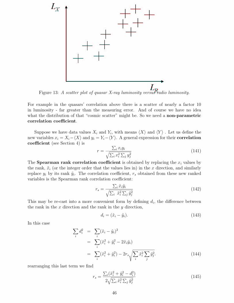
Figure 13: A scatter plot of quasar X-ray luminosity versus radio luminosity.

For example in the quasars’ correlation above there is a scatter of nearly a factor 10in luminosity - far greater than the measuring error. And of course we have no ideawhat the distribution of that “cosmic scatter” might be. So we need a non-parametriccorrelation coefficient.

Suppose we have data values Xi and Yi, with means 〈X〉 and 〈Y 〉 . Let us define thenew variables xi = Xi−〈X〉 and yi = Yi−〈Y 〉. A general expression for their correlationcoefficient (see Section 4) is

r =

∑

i xiyi√

∑

i x2i

∑

j y2j

(141)

The Spearman rank correlation coefficient is obtained by replacing the xi values bythe rank, xi (or the integer order that the values lies in) in the x direction, and similarlyreplace yi by its rank yi. The correlation coefficient, rs obtained from these new rankedvariables is the Spearman rank correlation coefficient:

rs =

∑

i xiyi√

∑

i x2i

∑

j y2j

(142)

This may be re-cast into a more convenient form by defining di, the difference betweenthe rank in the x direction and the rank in the y direction,

di = (xi − yi). (143)

In this case∑

i

d2i =

∑

i

(xi − yi)2

=∑

i

(x2i + y2

i − 2xiyi)

=∑

i

(x2i + y2

i ) − 2rs

√

∑

i

x2i

∑

j

y2j . (144)

rearranging this last term we find

rs =

∑

i(x2i + y2

i − d2i )

2√

∑

i x2i

∑

j y2j

(145)

46

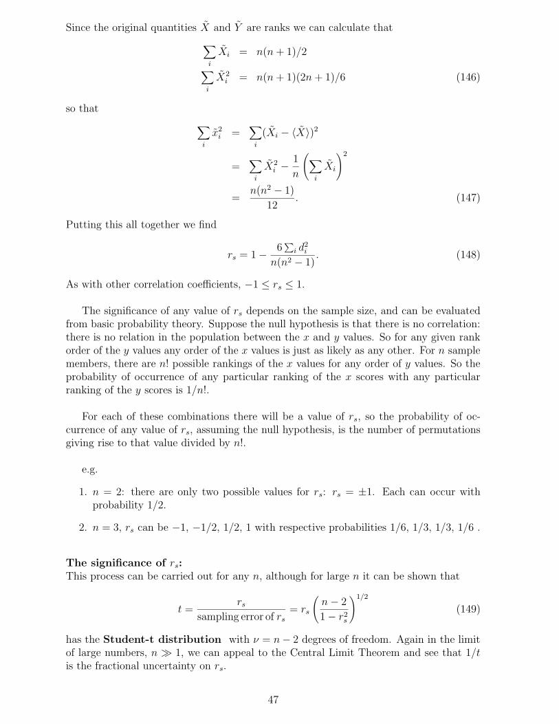
Since the original quantities X and Y are ranks we can calculate that

∑

i

Xi = n(n + 1)/2

∑

i

X2i = n(n + 1)(2n + 1)/6 (146)

so that

∑

i

x2i =

∑

i

(Xi − 〈X〉)2

=∑

i

X2i − 1

n

(

∑

i

Xi

)2

=n(n2 − 1)

12. (147)

Putting this all together we find

rs = 1 − 6∑

i d2i

n(n2 − 1). (148)

As with other correlation coefficients, −1 ≤ rs ≤ 1.

The significance of any value of rs depends on the sample size, and can be evaluatedfrom basic probability theory. Suppose the null hypothesis is that there is no correlation:there is no relation in the population between the x and y values. So for any given rankorder of the y values any order of the x values is just as likely as any other. For n samplemembers, there are n! possible rankings of the x values for any order of y values. So theprobability of occurrence of any particular ranking of the x scores with any particularranking of the y scores is 1/n!.

For each of these combinations there will be a value of rs, so the probability of oc-currence of any value of rs, assuming the null hypothesis, is the number of permutationsgiving rise to that value divided by n!.

e.g.

1. n = 2: there are only two possible values for rs: rs = ±1. Each can occur withprobability 1/2.

2. n = 3, rs can be −1, −1/2, 1/2, 1 with respective probabilities 1/6, 1/3, 1/3, 1/6 .

The significance of rs:This process can be carried out for any n, although for large n it can be shown that

t =rs

sampling error of rs

= rs

(

n − 2

1 − r2s

)1/2

(149)

has the Student-t distribution with ν = n − 2 degrees of freedom. Again in the limitof large numbers, n 1, we can appeal to the Central Limit Theorem and see that 1/tis the fractional uncertainty on rs.

47

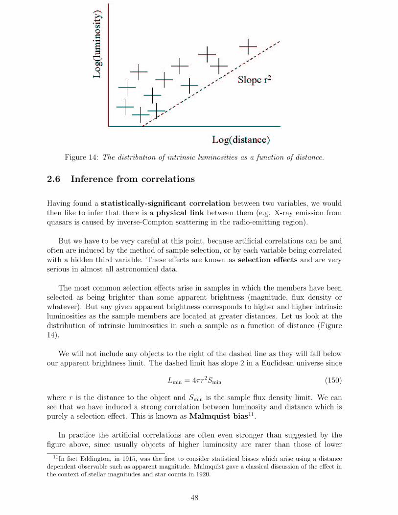
Figure 14: The distribution of intrinsic luminosities as a function of distance.

2.6 Inference from correlations

Having found a statistically-significant correlation between two variables, we wouldthen like to infer that there is a physical link between them (e.g. X-ray emission fromquasars is caused by inverse-Compton scattering in the radio-emitting region).

But we have to be very careful at this point, because artificial correlations can be andoften are induced by the method of sample selection, or by each variable being correlatedwith a hidden third variable. These effects are known as selection effects and are veryserious in almost all astronomical data.

The most common selection effects arise in samples in which the members have beenselected as being brighter than some apparent brightness (magnitude, flux density orwhatever). But any given apparent brightness corresponds to higher and higher intrinsicluminosities as the sample members are located at greater distances. Let us look at thedistribution of intrinsic luminosities in such a sample as a function of distance (Figure14).

We will not include any objects to the right of the dashed line as they will fall belowour apparent brightness limit. The dashed limit has slope 2 in a Euclidean universe since

Lmin = 4πr2Smin (150)

where r is the distance to the object and Smin is the sample flux density limit. We cansee that we have induced a strong correlation between luminosity and distance which ispurely a selection effect. This is known as Malmquist bias11.

In practice the artificial correlations are often even stronger than suggested by thefigure above, since usually objects of higher luminosity are rarer than those of lower

11In fact Eddington, in 1915, was the first to consider statistical biases which arise using a distancedependent observable such as apparent magnitude. Malmquist gave a classical discussion of the effect inthe context of stellar magnitudes and star counts in 1920.

48

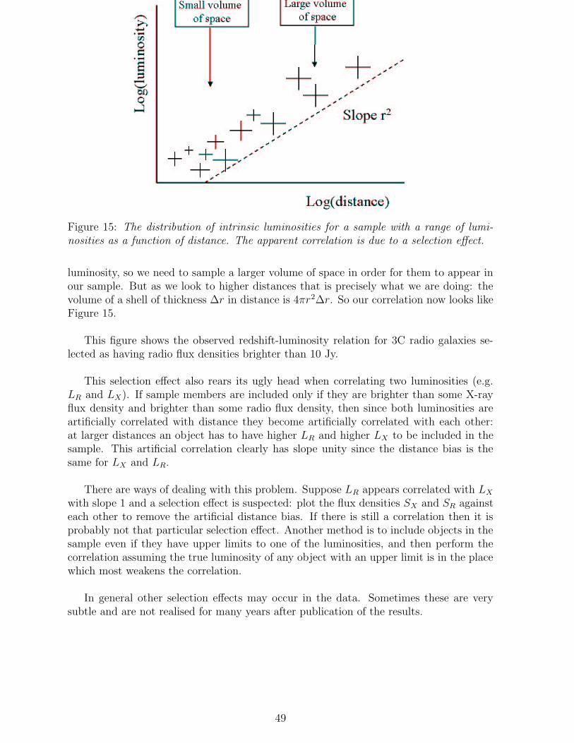
Figure 15: The distribution of intrinsic luminosities for a sample with a range of lumi-nosities as a function of distance. The apparent correlation is due to a selection effect.

luminosity, so we need to sample a larger volume of space in order for them to appear inour sample. But as we look to higher distances that is precisely what we are doing: thevolume of a shell of thickness ∆r in distance is 4πr2∆r. So our correlation now looks likeFigure 15.

This figure shows the observed redshift-luminosity relation for 3C radio galaxies se-lected as having radio flux densities brighter than 10 Jy.

This selection effect also rears its ugly head when correlating two luminosities (e.g.LR and LX). If sample members are included only if they are brighter than some X-rayflux density and brighter than some radio flux density, then since both luminosities areartificially correlated with distance they become artificially correlated with each other:at larger distances an object has to have higher LR and higher LX to be included in thesample. This artificial correlation clearly has slope unity since the distance bias is thesame for LX and LR.

There are ways of dealing with this problem. Suppose LR appears correlated with LX

with slope 1 and a selection effect is suspected: plot the flux densities SX and SR againsteach other to remove the artificial distance bias. If there is still a correlation then it isprobably not that particular selection effect. Another method is to include objects in thesample even if they have upper limits to one of the luminosities, and then perform thecorrelation assuming the true luminosity of any object with an upper limit is in the placewhich most weakens the correlation.

In general other selection effects may occur in the data. Sometimes these are verysubtle and are not realised for many years after publication of the results.

49

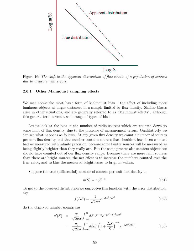
Figure 16: The shift in the apparent distribution of flux counts of a population of sourcesdue to measurement errors.

2.6.1 Other Malmquist sampling effects

We met above the most basic form of Malmquist bias – the effect of including moreluminous objects at larger distances in a sample limited by flux density. Similar biasesarise in other situations, and are generally referred to as “Malmquist effects”, althoughthis general term covers a wide range of types of bias.

Let us look at the bias in the number of radio sources which are counted down tosome limit of flux density, due to the presence of measurement errors. Qualitatively wecan see what happens as follows. At any given flux density we count a number of sourcesper unit flux density, but that number contains sources that shouldn’t have been countedhad we measured with infinite precision, because some fainter sources will be measured asbeing slightly brighter than they really are. But the same process also scatters objects weshould have counted out of our flux density range. Because there are more faint sourcesthan there are bright sources, the net effect is to increase the numbers counted over thetrue value, and to bias the measured brightnesses to brighter values.

Suppose the true (differential) number of sources per unit flux density is

n(S) = noS−α. (151)

To get to the observed distribution we convolve this function with the error distribution,say

f(∆S) =1√2πσ

e−∆S2/2σ2

(152)

So the observed number counts are

n′(S) =n0√2πσ

∫ ∞

−∞dS ′ S ′−αe−(S′−S)2/2σ2

=n0√2πσ

∫ ∞

−∞d∆S

(

1 +∆S

S

)−α

e−∆S2/2σ2

. (153)

50

For small ∆S S, we can expand the brackets in the second line

n′(S) = n(S)∫ ∞

−∞d∆S

(

1 +α∆S

S+

α(α − 1)∆S2

2S2+ · · ·

)

e−∆S2/2σ2

√2πσ

(154)

The integral of the first term is unity; the second term is zero because 〈∆S〉 = 0, and thethird term, with 〈∆S2〉 = σ2, gives approximately the effect of Malmquist bias:

∆n =α(α − 1)σ2

2S2n(S) (155)

or

∆ ln n =∆n

n=

α(α − 1)σ2

2S2(156)

This is the change in height of the log(n)−log(S) curve due to the presence of measurementerrors:

This shift is equivalent to a bias in the mean brightness of objects if they are selectedas having apparent brightness S ′;

∆ ln S ′ = −∆ ln n(S)

α

= −(α − 1)σ2

2S2(157)

or, in magnitudes (m = −2.5log10S)

∆m ≈ −5log10eαmσ2m

2S2(158)

if the measurement error in magnitudes is σm and the slope of the log(n) − m relation isαm = 0.4α.

2.6.2 Example: Malmquist bias in a quasar survey

A quasar survey has selected quasars with magnitudes B < 16.2 over 3 sr of sky, but withlarge measurement errors, σm ≈ 0.25. The slope of the log(n) − m relation for quasars isvery steep, due to cosmological evolution, and has a value αm ≈ 0.9. Hence the quasarswhich are found in the survey are, on average, measured as being about 0.07 magnitudesbrighter than they really are, and the number of quasars found is a factor about 40% toohigh.

51

2.7 Monte-Carlo Methods

To finish with, we shall consider an alternative approach to error analysis which has grownwith the availability of fast computing. Many of the analytic approaches to probability andstatistics we have developed in this course have made use of the Central Limit Theorem.This has allowed us simplify the problem to that of the study of the Gaussian distribution,which we understand well.

However, in many cases the Central Limit Theorem may not apply (we may not haveenough samples to approach the limit of n → ∞) or we may not believe the underlyingdistribution is a Gaussian, but still want to estimate confidence regions. Or it may justbe that we have a very complicated system for which it is hopeless to try and propagateall of the uncertainties analytically.

To deal with such circumstances, astronomers have turned to a set of methods called“Monte-Carlo” methods12. The idea here is that we make an ensemble of computerrealizations of whatever system we are studying. For each member of the ensemble, thecomponents of the system are randomly chosen from each of their underlying distributions.

For example, say we want to model realistic errors on the variance on different scales,estimated from Cosmic Microwave Background (CMB) sky, as seen by some particularexperiment. We would randomly generate a random temperature field with Gaussiantemperature variations, on a pixelized sky (lets not worry how, but it is quite easy).We might then want to add foreground microwave emission due to synchrotron radiationgenerated in our Galaxy. There may be uncertainties on this foreground which we couldmodel by sampling each pixel value from another distribution, maybe another Gaussian.Then we would add noise appropriate to the instrumental response in each pixel, samplingthe noise from e.g. again a Gaussian with a variance equal to the variance due to noise inthe instrument. We could build up a model for the observed CMB fluctuations by addingmore and more layers. We can generate an ensemble of such observations by repeatingthis process, but selecting each effect at random from its distribution each time.

Having generated such an ensemble, it can then be used to generate estimates of theCMB variance on different scales including all of these effects without having to appealto the Central Limit Theorem. The ensemble of estimated variances can then be used toestimate the distribution of measured variances, including all of these effects, and hencethe uncertainty of a measurement.

As neat as this sounds, and it can be very useful for modelling the statistical propertiesof non-Gaussian and nonlinear effects, we should note some limitations of the Monte-Carlomethod. The most basic is that we must make many choices about what the underlyingdistributions actually are. If we understand things well, this can be fine. But, as is quiteoften, if we don’t a simple Gaussian will be chosen. We should also be aware that we willneglect all of the things we don’t know about, for example systematics effects.

12The name “Monte-Carlo” comes from the emergence of the method during card games at Los Alamosduring the making of the atomic bomb, when the mathematician John von Neumann realized suchmethods would help him win.

52