Asymptotic properties of nonlinear estimates in

stochastic models with finite design space

Luc Pronzato

To cite this version:

Luc Pronzato. Asymptotic properties of nonlinear estimates in stochastic models with fi-nite design space. Statistics and Probability Letters, Elsevier, 2009, 79, pp.2307-2313.<10.1016/j.spl.2009.07.025>. <hal-00416008>

HAL Id: hal-00416008

https://hal.archives-ouvertes.fr/hal-00416008

Submitted on 11 Sep 2009

HAL is a multi-disciplinary open accessarchive for the deposit and dissemination of sci-entific research documents, whether they are pub-lished or not. The documents may come fromteaching and research institutions in France orabroad, or from public or private research centers.

L’archive ouverte pluridisciplinaire HAL, estdestinee au depot et a la diffusion de documentsscientifiques de niveau recherche, publies ou non,emanant des etablissements d’enseignement et derecherche francais ou etrangers, des laboratoirespublics ou prives.

Asymptotic properties of nonlinear estimates in stochastic models

with finite design spaceI

Luc Pronzato

Laboratoire I3S, CNRS/Universite de Nice-Sophia AntipolisBat. Euclide, Les Algorithmes, 2000 route des lucioles, BP 121

06903 Sophia Antipolis cedex, France

Abstract

Under the condition that the design space is finite, new sufficient conditions for the

strong consistency and asymptotic normality of the least-squares estimator in nonlin-

ear stochastic regression models are derived. Similar conditions are obtained for the

maximum-likelihood estimator in Bernoulli type experiments. Consequences on the se-

quential design of experiments are pointed out.

Key words: stochastic regressors, strong consistency, asymptotic normality, sequential

design, Bernoulli trials

1. Introduction and motivation

Consider a nonlinear regression model with observations

Yi = Y (xi) = η(xi, θ) + εi , (1)

where {εi} is a martingale difference sequence with respect to an increasing sequence of

σ-fields Fi such that supi IE{ε2i |Fi−1} < ∞ almost surely (a.s.), and η(x, θ) is a known

function of a parameter vector θ ∈ Θ (a compact subset of Rp) and a design variable

x ∈ X (a compact subset of Rd). Here θ denotes the unknown true value of θ and we

assume that θ is in the interior of Θ. The martingale difference sequence assumption

IThis work was partly accomplished while the author was invited at the Isaac Newton Institute forMathematical Sciences, Cambridge, UK, in July 2008. The support of the Newton Institute and of CNRSare gratefully acknowledged.

Email address: pronzato@i3s.unice.fr (Luc Pronzato)

Preprint submitted to Statistics & Probability Letters July 29, 2009

for {εi} in (1) is rather common in a stochastic control framework. It covers situations

where εi = hi δi with hi being a measurable function of past ε and {δi} forming an i.i.d.

sequence with zero mean also independent of past ε. A typical example is given by ARCH

(autoregressive conditionally heteroscedastic) processes.

The strong consistency of the Least-Squares (LS) estimator θn that minimizes

Sn(θ) =n∑

k=1

[Y (xk)− η(xk, θ)]2 (2)

is established in (Jennrich, 1969) in the case where εi are independent identically dis-

tributed (i.i.d.) errors with unknown variance σ2 and xi are non-random constants, under

the assumption that (1/n)Dn(θ, θ′) converges uniformly to a continuous function J(θ, θ′)

with J(θ, θ′) > 0 for all θ 6= θ′, where

Dn(θ, θ′) =n∑

i=1

[η(xi, θ)− η(xi, θ′)]2 . (3)

In a linear regression model, where η(x, θ) = f>(x)θ with f(x) a p-dimensional vector,

the condition above is equivalent to (1/n)X>n Xn → M , with M some positive definite

matrix and X = [f(x1), . . . , f(xn)]>, a condition thus much stronger than the well-known

condition for weak and strong consistency of θn

(X>n Xn)−1 → 0 , (4)

see, e.g., Lai et al. (1978); Lai and Wei (1982). The analogue of (4) for nonlinear regression

would be Dn(θ, θ′) → ∞ for all θ 6= θ′ . This condition is shown in (Wu, 1981) to be

necessary for the existence of a weakly consistent estimator of θ when εi are supposed to

be i.i.d. with a positive almost everywhere and absolutely continuous density with finite

Fisher information. It is also shown in the same paper to be sufficient for the (weak and

strong) consistency of the nonlinear LS estimator θn when Θ is a finite set. When Θ is a

compact set of Rp, it is complemented by additional assumptions to establish the strong

consistency of θn, see Th. 3 in (Wu, 1981).

Suppose now that xi is a Fi−1 measurable random variable. The motivation we have

in mind corresponds to adaptive experimental design, where the design point xi at step i

2

depends on observations Y1, . . . , Yi−1 through the estimate θi−1. Lai and Wei (1982) show

that the conditions

λmin[X>n Xn] →∞ a.s. (5)

{log λmax[X>n Xn]}ρ = o

(λmin[X

>n Xn]

)a.s. for some ρ > 1 , (6)

are sufficient for the strong consistency of θn in the model (1) with η(x, θ) linear in θ, i.e.

η(x, θ) = f>(x)θ, and stochastic regressors f(xi) (Example 1 in the same paper shows that

these conditions are in some sense weakest possible). Here and in what follows we denote

by λmin(M) and λmax(M) the minimum and maximum eigenvalues of a p× p matrix M.

The case of nonlinear stochastic regression models is considered in (Lai, 1994), where suf-

ficient conditions for strong consistency are given, which reduce to (5) and the Christopeit

and Helmes (1980) condition, λmax[X>n Xn] = O{λρ

min[X>n Xn]} a.s. for some ρ ∈ (1, 2) ,

in the case of a linear model.

It is the purpose of this paper to show that when the design space X is finite, a sufficient

condition for the strong consistency of θn in the model (1) is that with probability one

Dn(θ, θ′) →∞ faster than (log n)ρ for all θ 6= θ′ for some ρ > 1, a condition equivalent to

(5, 6) for linear models and much weaker than the conditions of Jennrich (1969) or Lai

(1994) for nonlinear models. Under the additional assumption

limi→∞

IE{ε2i |Fi−1} = σ2 a.s. for some constant σ , (7)

we also give a sufficient condition for the asymptotic normality of θn in (1). It should be

noticed that the assumption that X is finite is seldom limitative in situations where the

experiment is designed since practical considerations often impose such a restriction on

possible choices for xi. This is especially true for clinical trials where only certain doses

of the treatment are available, see Sect. 4 and Pronzato (2009b). Although less natural in

a stochastic control context where xi denotes the system input at time i, the assumption

that X is finite is satisfied when a suitable quantization is applied to the input sequence.

It can be contrasted with the less natural assumption that the admissible parameter set

Θ is finite, see, e.g., Caines (1975).

3

Sect. 2 concerns the strong consistency of θn and Sect. 3 its asymptotic normality.

The results obtained, which rely on a repeated sampling principle that can be used when

X is finite, are of rather general applicability and Sect. 4 concerns Maximum Likelihood

(ML) estimation in Bernoulli trials. Sect. 5 concludes and points out consequences on

sequentially designed experiments. We respectively denotea.s.→,

p→ andd→ almost sure

convergence, convergence in probability and in distribution. For M a p × p matrix, we

use the matrix norm ‖M‖ = sup‖u‖=1 ‖Mu‖ ≤ p maxi,j |{M}ij|.

2. Strong consistency of the nonlinear LS estimator when X is finite

Next theorem shows that the strong consistency of θn in (1) is a consequence of Dn(θ, θ)

tending to infinity fast enough for ‖θ − θ‖ ≥ δ > 0. The fact that the design space Xis finite makes the required rate of increase for Dn(θ, θ) quite slow. The result is valid

whether xi are non-random constants or are Fi−1-measurable random variables.

Theorem 1. Suppose that X is a finite set. If Dn(θ, θ) given by (3) satisfies

for all δ > 0 ,

[inf

‖θ−θ‖≥δ/τn

Dn(θ, θ)

]/(log n)ρ a.s.→∞ (n →∞) , for some ρ > 1 , (8)

with {τn} a nondecreasing sequence of positive deterministic constants, then the LS esti-

mator θn in the model (1) satisfies

τn‖θn − θ‖ a.s.→ 0 (n →∞) . (9)

Proof. The first part of the proof is based on Lemma 1 in (Wu, 1981). Suppose that (9)

is not satisfied. It implies that exists δ > 0 such that

Pr(lim supn→∞

τn‖θn − θ‖ ≥ δ) > 0 . (10)

Since Sn(θn) ≤ Sn(θ), (10) implies Pr(lim infn→∞ inf‖θ−θ‖≥δ/τn[Sn(θ) − Sn(θ)] ≤ 0) > 0 .

Therefore,

lim infn→∞

inf‖θ−θ‖≥δ/τn

[Sn(θ)− Sn(θ)] > 0 a.s. for any δ > 0 (11)

4

implies (9). The second part consists in establishing a sufficient condition for (11) based

on the growth rate of Dn(θ, θ). Denote In(x) = {i ∈ {1, . . . , n} : xi = x}. We have

Sn(θ)− Sn(θ) ≥ Dn(θ, θ)

1− 2

∑x∈X

∣∣∣∑i∈In(x) εi

∣∣∣ |η(x, θ)− η(x, θ)|Dn(θ, θ)

.

Under the condition (8), it thus suffices to prove that

lim supn→∞

sup‖θ−θ‖≥δ/τn

∑x∈X

∣∣∣∑i∈In(x) εi

∣∣∣ |η(x, θ)− η(x, θ)|Dn(θ, θ)

= 0 a.s. for any δ > 0 (12)

to obtain (11) and thus (9). Denote ui(x) the variable defined by ui(x) = 1 if x = xi

and ui(x) = 0 otherwise, so that∑n

i=1 ui(x) =∑n

i=1 u2i (x) = rn(x), the number of

times x appears in the sequence x1, . . . , xn. Notice that ui(x) is Fi−1-measurable. Since

Dn(θ, θ) ≥ D1/2n (θ, θ)r

1/2n (x)|η(x, θ)− η(x, θ)| for all x in X , we have

∑x∈X

∣∣∣∑i∈In(x) εi

∣∣∣ |η(x, θ)− η(x, θ)|Dn(θ, θ)

≤ 1

D1/2n (θ, θ)

∑x∈X

|∑ni=1 ui(x)εi|

[∑n

i=1 u2i (x)]

1/2.

Moreover, An(x) = |∑ni=1 ui(x)εi| [

∑ni=1 u2

i (x)]−1/2

is a.s. finite if rn(x) is finite and

limn→∞

|∑ni=1 ui(x)εi|

[∑n

i=1 u2i (x)]

1/2[log

∑ni=1 u2

i (x)]α

= 0 a.s.

for every α > 1/2 otherwise, see Lemma 2-(iii) of Lai and Wei (1982) and Corollary 7 of

Chow (1965). Since∑n

i=1 u2i (x) ≤ n for all x, (8) implies (12), which concludes the proof.

Remark 1. The case where the errors εi in (1) are i.i.d. with finite variance σ2 is consid-

ered in (Pronzato, 2009a). An(x) is then asymptotically normalN (0, σ2) when rn(x) →∞and, using the law of the iterated logarithm, we obtain (9) under the weaker condition

for all δ > 0 ,

[inf

‖θ−θ‖≥δ/τn

Dn(θ, θ)

]/(log log n)

a.s.→∞ (n →∞) , (13)

see also Th. 3 below. Under the same assumption of i.i.d. errors with finite variance and

using a similar approach, we also obtain in (Pronzato, 2009a) that θn is weakly consistent

5

when Dn(θ, θ)p→ ∞ for all θ 6= θ as n → ∞, which can be extended to τn‖θn − θ‖ p→ 0

when inf‖θ−θ‖≥δ/τnDn(θ, θ)

p→ ∞ for all δ > 0. The same property still holds when {εi}in (1) is a martingale difference sequence that satisfies (7) and rn(x), the number of times

x appears in the sequence x1, . . . , xn, satisfies rn(x)/IE{rn(x)} p→ 1 for all x ∈ X . In that

case, (9) can be obtained under a slightly weaker condition than (8) using results on the

law of the iterated logarithm for martingales, see Hall and Heyde (1980, Chap. 4).

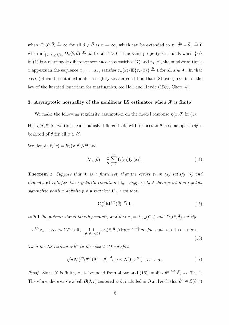
3. Asymptotic normality of the nonlinear LS estimator when X is finite

We make the following regularity assumption on the model response η(x, θ) in (1):

Hη: η(x, θ) is two times continuously differentiable with respect to θ in some open neigh-

borhood of θ for all x ∈ X .

We denote fθ(x) = ∂η(x, θ)/∂θ and

Mn(θ) =1

n

n∑i=1

fθ(xi)f>θ (xi) . (14)

Theorem 2. Suppose that X is a finite set, that the errors εi in (1) satisfy (7) and

that η(x, θ) satisfies the regularity condition Hη. Suppose that there exist non-random

symmetric positive definite p× p matrices Cn such that

C−1n M1/2

n (θ)p→ I , (15)

with I the p-dimensional identity matrix, and that cn = λmin(Cn) and Dn(θ, θ) satisfy

n1/4cn →∞ and ∀δ > 0 , inf‖θ−θ‖≥c2nδ

Dn(θ, θ)/(log n)ρ a.s.→∞ for some ρ > 1 (n →∞) .

(16)

Then the LS estimator θn in the model (1) satisfies

√nM1/2

n (θn)(θn − θ)d→ ω ∼ N (0, σ2I) , n →∞ . (17)

Proof. Since X is finite, cn is bounded from above and (16) implies θn a.s.→ θ, see Th. 1.

Therefore, there exists a ball B(θ, r) centered at θ, included in Θ and such that θn ∈ B(θ, r)

6

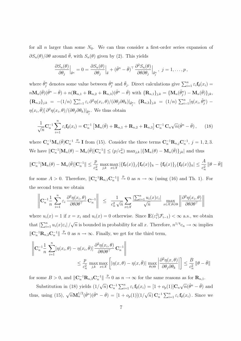
for all n larger than some N0. We can thus consider a first-order series expansion of

∂Sn(θ)/∂θ around θ, with Sn(θ) given by (2). This yields

∂Sn(θ)

∂θj

∣∣∣θn

= 0 =∂Sn(θ)

∂θj

∣∣∣θ+ (θn − θ)>

∂2Sn(θ)

∂θ∂θj

∣∣∣θnj

, j = 1, . . . , p ,

where θnj denotes some value between θn

j and θj. Direct calculations give∑n

i=1 εifθ(xi) =

nMn(θ)(θn − θ) + n(Rn,1 + Rn,2 + Rn,3)(θn − θ) with {Rn,1}j,k = {Mn(θn

j ) −Mn(θ)}jk,

{Rn,2}j,k = −(1/n)∑n

i=1 εi ∂2η(xi, θ)/(∂θj∂θk)|θn

j, {Rn,3}j,k = (1/n)

∑ni=1[η(xi, θ

nj ) −

η(xi, θ)] ∂2η(xi, θ)/(∂θj∂θk)|θn

j. We thus obtain

1√nC−1

n

n∑i=1

εifθ(xi) = C−1n

[Mn(θ) + Rn,1 + Rn,2 + Rn,3

]C−1

n Cn

√n(θn − θ) , (18)

where C−1n Mn(θ)C−1

n

p→ I from (15). Consider the three terms C−1n Rn,jC

−1n , j = 1, 2, 3.

We have ‖C−1n [Mn(θ)−Mn(θ)]C−1

n ‖ ≤ (p/c2n) maxj,k |{Mn(θ)−Mn(θ)}jk| and thus

‖C−1n [Mn(θ)−Mn(θ)]C−1

n ‖ ≤ p

c2n

maxj,k

maxx∈X

|{fθ(x)}j{fθ(x)}k − {fθ(x)}j{fθ(x)}k| ≤ A

c2n

‖θ − θ‖

for some A > 0. Therefore, ‖C−1n Rn,1C

−1n ‖ p→ 0 as n → ∞ (using (16) and Th. 1). For

the second term we obtain∥∥∥∥∥C−1

n

1

n

n∑i=1

εi∂2η(xi, θ)

∂θ∂θ>C−1

n

∥∥∥∥∥ ≤ 1

c2n

√n

∑x∈X

|∑ni=1 ui(x)εi|√

nmax

x∈X ,θ∈Θ

∥∥∥∥∂2η(xi, θ)

∂θ∂θ>

∥∥∥∥

where ui(x) = 1 if x = xi and ui(x) = 0 otherwise. Since IE(ε2i |Fi−1) < ∞ a.s., we obtain

that |∑ni=1 ui(x)εi| /

√n is bounded in probability for all x. Therefore, n1/4cn →∞ implies

‖C−1n Rn,2C

−1n ‖ p→ 0 as n →∞. Finally, we get for the third term,

∥∥∥∥∥C−1n

1

n

n∑i=1

[η(xi, θ)− η(xi, θ)]∂2η(xi, θ)

∂θ∂θ>C−1

n

∥∥∥∥∥

≤ p

c2n

maxj,k

maxx∈X

[|η(x, θ)− η(x, θ)| max

θ∈Θ

∣∣∣∣∂2η(x, θ)

∂θj∂θk

∣∣∣∣]≤ B

c2n

‖θ − θ‖

for some B > 0, and ‖C−1n Rn,3C

−1n ‖ p→ 0 as n →∞ for the same reasons as for Rn,1.

Substitution in (18) yields (1/√

n)C−1n

∑ni=1 εi fθ(xi) = [1 + op(1)]Cn

√n(θn − θ) and

thus, using (15),√

nM1/2n (θn)(θn − θ) = [1 + op(1)](1/

√n)C−1

n

∑ni=1 εi fθ(xi) . Since we

7

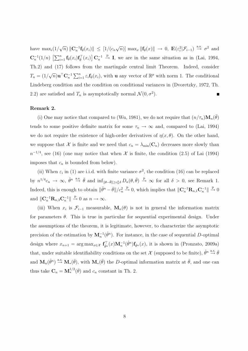
have maxi(1/√

n) ‖C−1n fθ(xi)‖ ≤ [1/(cn

√n)] maxx ‖fθ(x)‖ → 0, IE(ε2

i |Fi−1)a.s.→ σ2 and

C−1n (1/n)

[∑ni=1 fθ(xi)f

>θ

(xi)]C−1

n

p→ I, we are in the same situation as in (Lai, 1994,

Th.2) and (17) follows from the martingale central limit Theorem. Indeed, consider

Tn = (1/√

n)u>C−1n

∑ni=1 εifθ(xi), with u any vector of Rp with norm 1. The conditional

Lindeberg condition and the condition on conditional variances in (Dvoretzky, 1972, Th.

2.2) are satisfied and Tn is asymptotically normal N (0, σ2).

Remark 2.

(i) One may notice that compared to (Wu, 1981), we do not require that (n/τn)Mn(θ)

tends to some positive definite matrix for some τn → ∞ and, compared to (Lai, 1994)

we do not require the existence of high-order derivatives of η(x, θ). On the other hand,

we suppose that X is finite and we need that cn = λmin(Cn) decreases more slowly than

n−1/4, see (16) (one may notice that when X is finite, the condition (2.5) of Lai (1994)

imposes that cn is bounded from below).

(ii) When εi in (1) are i.i.d. with finite variance σ2, the condition (16) can be replaced

by n1/4cn → ∞, θn a.s.→ θ and inf‖θ−θ‖≥c2nδ Dn(θ, θ)p→ ∞ for all δ > 0, see Remark 1.

Indeed, this is enough to obtain ‖θn− θ‖/c2n

p→ 0, which implies that ‖C−1n Rn,1C

−1n ‖ p→ 0

and ‖C−1n Rn,3C

−1n ‖ p→ 0 as n →∞.

(iii) When xi is Fi−1 measurable, Mn(θ) is not in general the information matrix

for parameters θ. This is true in particular for sequential experimental design. Under

the assumptions of the theorem, it is legitimate, however, to characterize the asymptotic

precision of the estimation by M−1n (θn). For instance, in the case of sequential D-optimal

design where xn+1 = arg maxx∈X f>θn(x)M−1

n (θn)fθn(x), it is shown in (Pronzato, 2009a)

that, under suitable identifiability conditions on the set X (supposed to be finite), θn a.s.→ θ

and Mn(θn)a.s.→ M∗(θ), with M∗(θ) the D-optimal information matrix at θ, and one can

thus take Cn = M1/2∗ (θ) and cn constant in Th. 2.

8

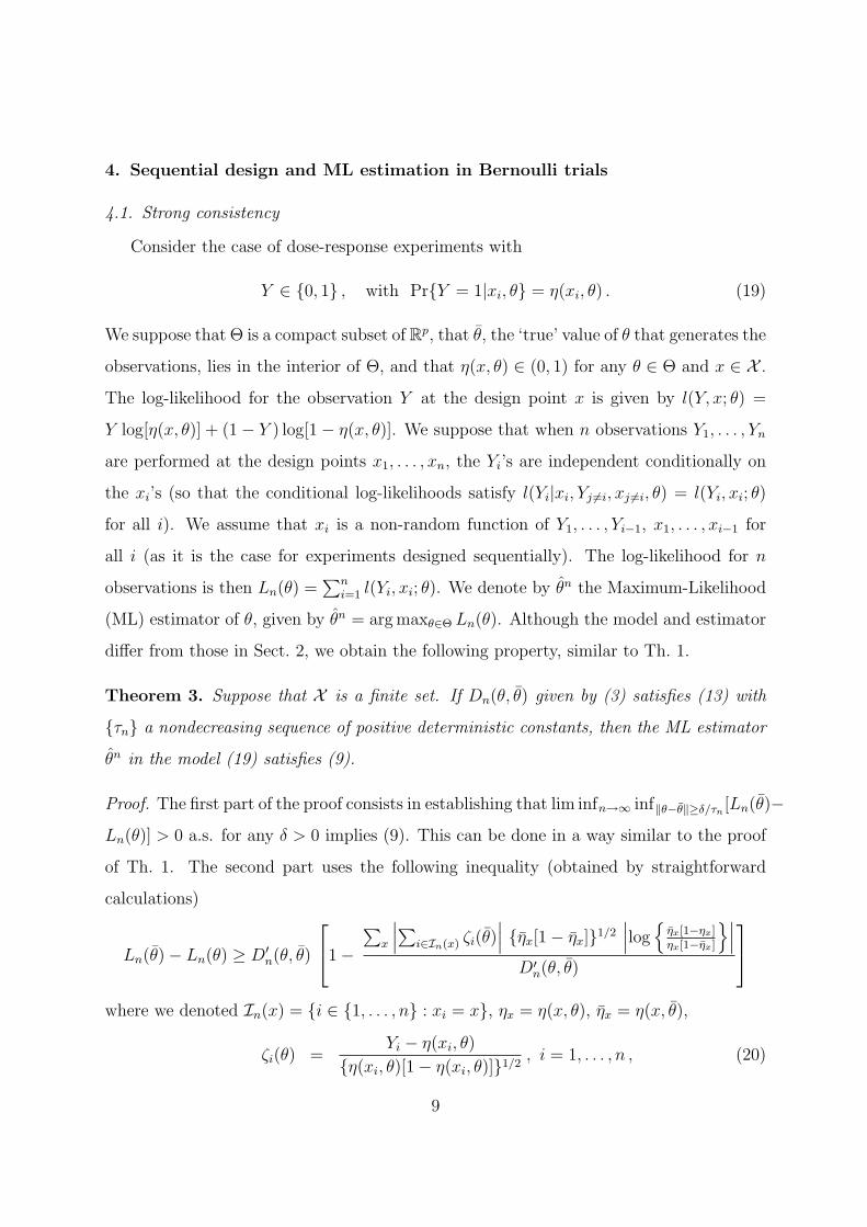
4. Sequential design and ML estimation in Bernoulli trials

4.1. Strong consistency

Consider the case of dose-response experiments with

Y ∈ {0, 1} , with Pr{Y = 1|xi, θ} = η(xi, θ) . (19)

We suppose that Θ is a compact subset of Rp, that θ, the ‘true’ value of θ that generates the

observations, lies in the interior of Θ, and that η(x, θ) ∈ (0, 1) for any θ ∈ Θ and x ∈ X .

The log-likelihood for the observation Y at the design point x is given by l(Y, x; θ) =

Y log[η(x, θ)] + (1− Y ) log[1− η(x, θ)]. We suppose that when n observations Y1, . . . , Yn

are performed at the design points x1, . . . , xn, the Yi’s are independent conditionally on

the xi’s (so that the conditional log-likelihoods satisfy l(Yi|xi, Yj 6=i, xj 6=i, θ) = l(Yi, xi; θ)

for all i). We assume that xi is a non-random function of Y1, . . . , Yi−1, x1, . . . , xi−1 for

all i (as it is the case for experiments designed sequentially). The log-likelihood for n

observations is then Ln(θ) =∑n

i=1 l(Yi, xi; θ). We denote by θn the Maximum-Likelihood

(ML) estimator of θ, given by θn = arg maxθ∈Θ Ln(θ). Although the model and estimator

differ from those in Sect. 2, we obtain the following property, similar to Th. 1.

Theorem 3. Suppose that X is a finite set. If Dn(θ, θ) given by (3) satisfies (13) with

{τn} a nondecreasing sequence of positive deterministic constants, then the ML estimator

θn in the model (19) satisfies (9).

Proof. The first part of the proof consists in establishing that lim infn→∞ inf‖θ−θ‖≥δ/τn[Ln(θ)−

Ln(θ)] > 0 a.s. for any δ > 0 implies (9). This can be done in a way similar to the proof

of Th. 1. The second part uses the following inequality (obtained by straightforward

calculations)

Ln(θ)− Ln(θ) ≥ D′n(θ, θ)

1−

∑x

∣∣∣∑i∈In(x) ζi(θ)∣∣∣ {ηx[1− ηx]}1/2

∣∣∣log{

ηx[1−ηx]ηx[1−ηx]

}∣∣∣D′

n(θ, θ)

where we denoted In(x) = {i ∈ {1, . . . , n} : xi = x}, ηx = η(x, θ), ηx = η(x, θ),

ζi(θ) =Yi − η(xi, θ)

{η(xi, θ)[1− η(xi, θ)]}1/2, i = 1, . . . , n , (20)

9

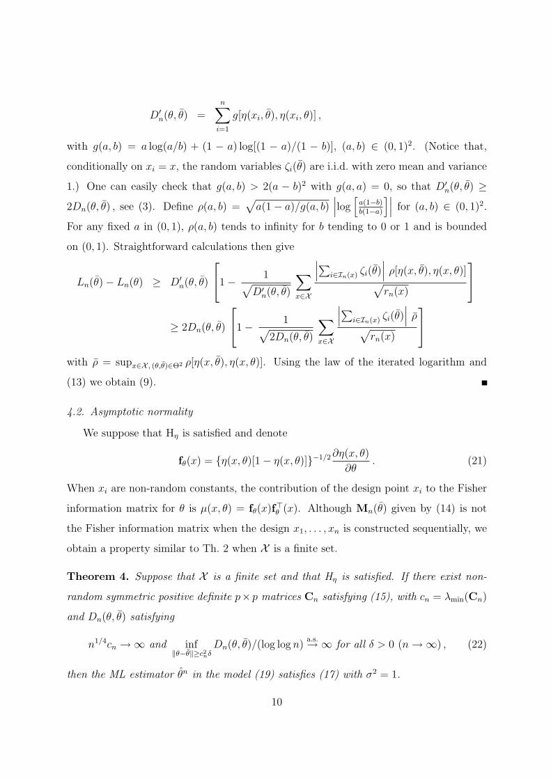
D′n(θ, θ) =

n∑i=1

g[η(xi, θ), η(xi, θ)] ,

with g(a, b) = a log(a/b) + (1 − a) log[(1 − a)/(1 − b)], (a, b) ∈ (0, 1)2. (Notice that,

conditionally on xi = x, the random variables ζi(θ) are i.i.d. with zero mean and variance

1.) One can easily check that g(a, b) > 2(a − b)2 with g(a, a) = 0, so that D′n(θ, θ) ≥

2Dn(θ, θ) , see (3). Define ρ(a, b) =√

a(1− a)/g(a, b)∣∣∣log

[a(1−b)b(1−a)

]∣∣∣ for (a, b) ∈ (0, 1)2.

For any fixed a in (0, 1), ρ(a, b) tends to infinity for b tending to 0 or 1 and is bounded

on (0, 1). Straightforward calculations then give

Ln(θ)− Ln(θ) ≥ D′n(θ, θ)

1− 1√

D′n(θ, θ)

∑x∈X

∣∣∣∑i∈In(x) ζi(θ)∣∣∣ ρ[η(x, θ), η(x, θ)]

√rn(x)

≥ 2Dn(θ, θ)

1− 1√

2Dn(θ, θ)

∑x∈X

∣∣∣∑i∈In(x) ζi(θ)∣∣∣ ρ

√rn(x)

with ρ = supx∈X , (θ,θ)∈Θ2 ρ[η(x, θ), η(x, θ)]. Using the law of the iterated logarithm and

(13) we obtain (9).

4.2. Asymptotic normality

We suppose that Hη is satisfied and denote

fθ(x) = {η(x, θ)[1− η(x, θ)]}−1/2∂η(x, θ)

∂θ. (21)

When xi are non-random constants, the contribution of the design point xi to the Fisher

information matrix for θ is µ(x, θ) = fθ(x)f>θ (x). Although Mn(θ) given by (14) is not

the Fisher information matrix when the design x1, . . . , xn is constructed sequentially, we

obtain a property similar to Th. 2 when X is a finite set.

Theorem 4. Suppose that X is a finite set and that Hη is satisfied. If there exist non-

random symmetric positive definite p×p matrices Cn satisfying (15), with cn = λmin(Cn)

and Dn(θ, θ) satisfying

n1/4cn →∞ and inf‖θ−θ‖≥c2nδ

Dn(θ, θ)/(log log n)a.s.→∞ for all δ > 0 (n →∞) , (22)

then the ML estimator θn in the model (19) satisfies (17) with σ2 = 1.

10

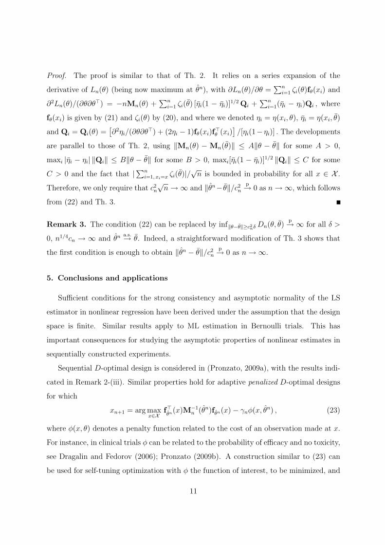
Proof. The proof is similar to that of Th. 2. It relies on a series expansion of the

derivative of Ln(θ) (being now maximum at θn), with ∂Ln(θ)/∂θ =∑n

i=1 ζi(θ)fθ(xi) and

∂2Ln(θ)/(∂θ∂θ>) = −nMn(θ) +∑n

i=1 ζi(θ) [ηi(1 − ηi)]1/2 Qi +

∑ni=1(ηi − ηi)Qi , where

fθ(xi) is given by (21) and ζi(θ) by (20), and where we denoted ηi = η(xi, θ), ηi = η(xi, θ)

and Qi = Qi(θ) =[∂2ηi/(∂θ∂θ>) + (2ηi − 1)fθ(xi)f

>θ (xi)

]/[ηi(1− ηi)] . The developments

are parallel to those of Th. 2, using ‖Mn(θ) − Mn(θ)‖ ≤ A‖θ − θ‖ for some A > 0,

maxi |ηi − ηi| ‖Qi‖ ≤ B‖θ − θ‖ for some B > 0, maxi[ηi(1 − ηi)]1/2 ‖Qi‖ ≤ C for some

C > 0 and the fact that |∑ni=1, xi=x ζi(θ)|/

√n is bounded in probability for all x ∈ X .

Therefore, we only require that c2n

√n →∞ and ‖θn− θ‖/c2

n

p→ 0 as n →∞, which follows

from (22) and Th. 3.

Remark 3. The condition (22) can be replaced by inf‖θ−θ‖≥c2nδ Dn(θ, θ)p→∞ for all δ >

0, n1/4cn → ∞ and θn a.s.→ θ. Indeed, a straightforward modification of Th. 3 shows that

the first condition is enough to obtain ‖θn − θ‖/c2n

p→ 0 as n →∞.

5. Conclusions and applications

Sufficient conditions for the strong consistency and asymptotic normality of the LS

estimator in nonlinear regression have been derived under the assumption that the design

space is finite. Similar results apply to ML estimation in Bernoulli trials. This has

important consequences for studying the asymptotic properties of nonlinear estimates in

sequentially constructed experiments.

Sequential D-optimal design is considered in (Pronzato, 2009a), with the results indi-

cated in Remark 2-(iii). Similar properties hold for adaptive penalized D-optimal designs

for which

xn+1 = arg maxx∈X

f>θn(x)M−1

n (θn)fθn(x)− γnφ(x, θn) , (23)

where φ(x, θ) denotes a penalty function related to the cost of an observation made at x.

For instance, in clinical trials φ can be related to the probability of efficacy and no toxicity,

see Dragalin and Fedorov (2006); Pronzato (2009b). A construction similar to (23) can

be used for self-tuning optimization with φ the function of interest, to be minimized, and

11

f>θn(x)M−1

n (θn)fθn(x)/γn playing the role of a penalty for poor estimation, see Pronzato

(2000).

When γn in (23) is a non-random constant, under identifiability conditions on the set

X similar to those in (Pronzato, 2009a), and assuming that |φ(x, θ)| is bounded for all

x ∈ X (finite) and θ ∈ Θ, we obtain that θn is strongly consistent and asymptotically

normal. This remains true if γn is a Fn-measurable random variable (with Fn generated

by Y1, . . . , Yn) that tends a.s. to a non-random constant as n → ∞ (in particular, one

may take γn as a function of θn). Developments similar to those in (Pronzato, 2009a)

show that the strong consistency of θn is preserved when {γn} is a non-random increasing

sequence satisfying γn →∞ and γn(log log n)/n → 0 in model (1) with i.i.d. errors or in

model (19). For LS estimation in model (1) with {εi} a martingale difference sequence,

we require γn(log n)ρ/n → 0 for some ρ > 1, a condition similar to that obtained in

(Pronzato, 2000) when η(x, θ) is linear in θ (without the assumption that X is finite).

The details will be presented elsewhere. Asymptotic normality is difficult to establish

when γn → ∞ since there is no obvious choice for the matrices Cn of Th. 2 and 4. A

possible candidate is Cn = M1/2n (θ) with Mn(θ) the design matrix generated by iterations

similar to (23) but with θ substituted for θn.

Acknowledgments

The author wishes to thank the two referees for their careful reading and comments

that contributed to improve the readability of the paper.

References

Caines, P., 1975. A note on the consistency of maximum likelihood estimates for finite

families of stochastic processes. Annals of Statistics 3 (2), 539–546.

Chow, Y., 1965. Local convergence of martingales and the law of large numbers. Annals

of Math. Stat. 36, 552–558.

12

Christopeit, N., Helmes, K., 1980. Strong consistency of least squares estimators in linear

regression models. Annals of Statistics 8, 778–788.

Dragalin, V., Fedorov, V., 2006. Adaptive designs for dose-finding based on efficacy-

toxicity response. Journal of Statistical Planning and Inference 136, 1800–1823.

Dvoretzky, A., 1972. Asymptotic normality for sums of dependent random variables. In:

Proceedings of the Sixth Berkeley Symposium on Mathematical Statistics and Proba-

bility, Vol. II: Probability theory. Univ. California Press, Berkeley, Calif., pp. 513–535.

Hall, P., Heyde, C., 1980. Martingale Limit Theory and Its Applications. Academic Press,

New York.

Jennrich, R., 1969. Asymptotic properties of nonlinear least squares estimation. Annals

of Math. Stat. 40, 633–643.

Lai, T., 1994. Asymptotic properties of nonlinear least squares estimates in stochastic

regression models. Annals of Statistics 22 (4), 1917–1930.

Lai, T., Robbins, H., Wei, C., 1978. Strong consistency of least squares estimates in

multiple regression. Proc. Nat. Acad. Sci. USA 75 (7), 3034–3036.

Lai, T., Wei, C., 1982. Least squares estimates in stochastic regression models with ap-

plications to identification and control of dynamic systems. Annals of Statistics 10 (1),

154–166.

Pronzato, L., 2000. Adaptive optimisation and D-optimum experimental design. Annals

of Statistics 28 (6), 1743–1761.

Pronzato, L., 2009a. One-step ahead adaptive D-optimal design on a finite design space

is asymptotically optimal. Metrika (to appear, DOI: 10.1007/s00184-008-0227-y).

Pronzato, L., 2009b. Penalized optimal designs for dose-finding. Journal of Statistical

Planning and Inference (to appear, DOI: 10.1016/j.jspi.2009.07.012).

13

Wu, C., 1981. Asymptotic theory of nonlinear least squares estimation. Annals of Statistics

9 (3), 501–513.

14