Embed Size (px)
Citation preview
ASYMPTOTIC VARIANCE
OF THE BEURLING TRANSFORM
KARI ASTALA, OLEG IVRII, ANTTI PERALA, AND ISTVAN PRAUSE
Abstract. We study the interplay between infinitesimal deformationsof conformal mappings, quasiconformal distortion estimates and integralmeans spectra. By the work of McMullen, the second derivative of theHausdorff dimension of the boundary of the image domain is naturallyrelated to asymptotic variance of the Beurling transform. In view of atheorem of Smirnov which states that the dimension of a k-quasicircleis at most 1 + k2, it is natural to expect that the maximum asymptoticvariance Σ2 = 1. In this paper, we prove 0.87913 6 Σ2 6 1.
For the lower bound, we give examples of polynomial Julia sets whichare k-quasicircles with dimensions 1 + 0.87913 k2 for k small, therebyshowing that Σ2 > 0.87913. The key ingredient in this construction is agood estimate for the distortion k, which is better than the one given by astraightforward use of the λ-lemma in the appropriate parameter space.Finally, we develop a new fractal approximation scheme for evaluatingΣ2 in terms of nearly circular polynomial Julia sets.
1. Introduction
In his work on the Weil-Petersson metric [27], McMullen considered cer-
tain holomorphic families of conformal maps
ϕt : D∗ → C, ϕ0(z) = z, where D∗ = z : |z| > 1,
that naturally arise in complex dynamics and Teichmuller theory. For these
special families, he used thermodynamic formalism to relate a number of
different dynamical features. For instance, he showed that the infinitesimal
growth of the Hausdorff dimension of the Jordan curves ϕt(S1) is connected
2010 Mathematics Subject Classification. Primary 30C62; Secondary 30H30.Key words and phrases. Quasiconformal map, Beurling transform, Asymptotic vari-
ance, Bergman projection, Bloch space, Hausdorff dimension, Julia set.A.P. was supported by the Vilho, Yrjo and Kalle Vaisala Foundation and the Emil Aal-
tonen Foundation. I.P. and A.P. were supported by the Academy of Finland (SA) grants1266182 and 1273458. All authors were supported by the Center of Excellence Analysisand Dynamics, SA grants 75166001 and 12719831. Part of this research was performedwhile K.A. and I.P. were visiting the Institute for Pure and Applied Mathematics (IPAM),which is supported by the National Science Foundation.
1
2 K. ASTALA, O. IVRII, A. PERALA, AND I. PRAUSE
to the asymptotic variance of the first derivative of the vector field v =dϕtdt
∣∣t=0
by the formula
2d2
dt2
∣∣∣∣t=0
H. dim ϕt(S1) = σ2(v′), (1.1)
where the asymptotic variance of a Bloch function g in D∗ is given by
σ2(g) =1
2πlim supR→1+
1
| log(R− 1)|
ˆ|z|=R
|g(z)|2|dz|. (1.2)
This terminology is justified by viewing g as a stochastic process
Ys(ζ) = g((1− e−s)ζ), ζ ∈ S1, 0 6 s <∞,
with respect to the probability measure |dζ|/2π, in which case σ2(g) =
lim sups→∞1s σ
2Ys
. For further relevance of probability methods to the study
of the boundary distortion of conformal maps, we refer the reader to [17, 21].
For arbitrary families of conformal maps, the identity (1.1) may not hold.
For instance, Le and Zinsmeister [19] constructed a family ϕt for which
σ2(v′) is zero, while t 7→ M.dimϕt(S1) (with Hausdorff dimension replaced
by Minkowski dimension) is equal to 1 for t < 0 but grows quadratically for
t > 0.
Nevertheless, it is natural to enquire if McMullen’s formula (1.1) holds on
the level of universal bounds. As will be explained in detail in the subsequent
sections, for general holomorphic families of conformal maps ϕt parametrised
by a complex parameter t ∈ D, one can combine the work of Smirnov [41]
with the theory of holomorphic motions [23, 40] to show that
H.dim ϕt(S1) 6 1 +(1−
√1− |t|2)2
|t|2= 1 +
|t|2
4+O(|t|4), t ∈ D. (1.3)
It is conjectured that the equality in (1.3) holds for some family, but this is
still open. On the other hand, the derivative of the infinitesimal vector field
v = dϕtdt
∣∣t=0
can be represented in the form
v′ = Sµ
where |µ(z)| 6 χD and S is the Beurling transform , the principal value
integral
Sµ(z) = − 1
π
ˆC
µ(w)
(z − w)2dm(w). (1.4)
(Since the support of µ is contained in the unit disk, v′ is a holomorphic
function on the exterior unit disk.)
ASYMPTOTIC VARIANCE OF THE BEURLING TRANSFORM 3
In this formalism, McMullen’s identity describes the asymptotic variance
σ2(Sµ) for a “dynamical” Beltrami coefficient µ, which is invariant under a
co-compact Fuchsian group or a Blaschke product.
In this paper, we study the quantity
Σ2 := supσ2(Sµ) : |µ| 6 χD (1.5)
from several different perspectives. In addition to the problem of dimension
distortion of quasicircles, Σ2 is naturally related to questions on integral
means of conformal maps, which we discuss later in the introduction. The
first result in this work is an upper bound for Σ2:
Theorem 1.1. Suppose µ is measurable in C with |µ| 6 χD. Then,
σ2(Sµ) :=1
2πlim supR→1+
1
| log(R− 1)|
ˆ 2π
0|Sµ(Reiθ)|2 dθ 6 1. (1.6)
We give two different proofs for (1.6), one using holomorphic motions
and quasiconformal geometry in Section 4, and another based on complex
dynamics and fractal approximation in Section 6.
In view of McMullen’s identity and the possible sharpness of Smirnov’s
dimension bounds, it is natural to expect that the bound (1.6) is optimal
with Σ2 = 1, and in the first version of this paper we formulated a con-
jecture to that extent. However, after having read our manuscript, Hakan
Hedenmalm managed to show [12] that actually Σ2 < 1.
For lower bounds on Σ2, we produce examples in Section 5 showing:
Theorem 1.2. There exists a Beltrami coefficient |µ| 6 χD such that
σ2(Sµ) > 0.87913.
In fact, our construction gives new bounds for the quasiconformal distor-
tion of certain polynomial Julia sets:
Theorem 1.3. Consider the polynomials Pt(z) = zd + t z. For |t| < 1, the
Julia set J (Pt) is a Jordan curve which can be expressed as the image of the
unit circle by a k-quasiconformal map of C, where
k =d
1d−1
4|t|+O(|t|2).
4 K. ASTALA, O. IVRII, A. PERALA, AND I. PRAUSE
In particular, when d = 20 and |t| is small, k ≈ 0.585 · |t|2 and J (Pt) is a
k-quasicircle with
H. dim J (Pt) ≈ 1 + 0.87913 · k2. (1.7)
Note that the distortion estimates in Theorem 1.3 are strictly better (for
d > 3) than those given by a straightforward use of the λ-lemma. For a
detailed discussion, see Section 5. In terms of the dimension distortion of
quasicircles, Theorem 1.3 improves upon all previously known examples. For
instance, the holomorphic snowflake construction of [8] gives a k-quasicircle
of dimension ≈ 1 + 0.69 k2.
In order to further explicate the relationship between asymptotic variance
and dimension asymptotics, consider the function
D(k) = supH. dim Γ : Γ is a k-quasicircle, 0 6 k < 1.
The fractal approximation principle of Section 6 roughly says that infinites-
imally, it is sufficient to consider certain quasicircles, namely nearly circular
polynomial Julia sets. As a consequence, we prove:
Theorem 1.4.
Σ2 6 lim infk→0
D(k)− 1
k2. (1.8)
Together with Smirnov’s bound [41],
D(k) 6 1 + k2, (1.9)
Theorem 1.4 gives an alternative proof for Theorem 1.1. We note that the
function D(k) may be also characterised in terms of several other properties
in place of Hausdorff dimension, see [3]. It would be interesting to know if
the reverse inequality in Theorem 1.4 holds.
In Section 7, we study the fractal approximation question in the Fuchsian
setting. One may expect that it may be possible to approximate Σ2 using
Beltrami coefficients invariant under co-compact Fuchsian groups. However,
this turns out not to be the case. To this end, we show:
Theorem 1.5.
Σ2F := sup
µ∈MF, |µ|6χD
σ2(Sµ) < 2/3.
ASYMPTOTIC VARIANCE OF THE BEURLING TRANSFORM 5
Theorem 1.5 may be viewed as an upper bound for the quotient of the
Weil-Petersson and Teichmuller metrics, over all Teichmuller spaces Tg with
g > 2. (To make the bound genus-independent, one needs to normalise
the hyperbolic area of Riemann surfaces to be 1.) The proof follows from
simple duality arguments and the fact that there is a definite defect in the
Cauchy-Schwarz inequality.
Finally, we compare our problem with another method of embedding a
conformal map f into a flow:
log f ′t(z) = t log f ′(z), t ∈ D. (1.10)
In this case, the derivative of the infinitesimal vector field at t = 0 is just the
Bloch function log f ′(z). However, even if f itself is univalent, the univalence
of ft is only guaranteed for |t| 6 1/4, see [30]. One advantage of the notion
(1.5) and holomorphic flows parametrised by Beltrami equations is that they
do not suffer from this “univalency gap”.
In the case of domains bounded by regular fractals and the corresponding
equivariant Riemann mappings f(z), we have several interrelated dynamical
and geometric characteristics:
• The integral means spectrum of a conformal map:
βf (τ) = lim supr→1
log´|z|=r |(f
′)τ |dθlog 1
1−r, τ ∈ C. (1.11)
• The asymptotic variance a Bloch function g ∈ B:
σ2(g) = lim supr→1
1
2π| log(1− r)|
ˆ|z|=r
|g(z)|2dθ. (1.12)
• The LIL constant of a conformal map is defined as the essential
supremum of CLIL(f, θ) over θ ∈ [0, 2π) where
CLIL(f, θ) = lim supr→1
log |f ′(reiθ)|√log 1
1−r log log log 11−r
. (1.13)
Theorem 1.6. Suppose f(z) is a conformal map, such that the image of the
unit circle f(S1) is a Jordan curve, invariant under a hyperbolic conformal
dynamical system. Then,
2d2
dτ2
∣∣∣∣τ=0
βf (τ) = σ2(log f ′) = C2LIL(f), (1.14)
6 K. ASTALA, O. IVRII, A. PERALA, AND I. PRAUSE
where β(τ) is the integral means spectrum, σ2 is the asymptotic variance of
the Bloch function log f ′, and CLIL denotes the constant in the law of the
iterated logarithm (1.13).
We emphasise that the above quantities are not equal in general, but only
for special domains Ω that have fractal boundary. For these domains, the
limits in the definitions of βf (τ) and σ2(log f ′) exist, while CLIL(f, θ) is a
constant function (up to a set of measure 0).
The equalities in (1.14) are mediated by a fourth quantity involving the
dynamical asymptotic variance of a Holder continuous potential from ther-
modynamic formalism. The equality between the dynamical variance and
C2LIL is established in [35, 36], while the works [11, 22] give the connection
to the integral means β(τ). The missing link, it seems, is the connection
between the dynamical variance and σ2, which can be proved using a global
analogue of McMullen’s coboundary relation. Details will be given in Section
8. We note that an alternative approach connecting β(τ) and σ2 directly
has been considered in the special case of polynomial Julia sets, see [17].
With these connections in mind, we relate our quantity Σ2 to the universal
integral means spectrum B(τ) = supf βf (τ):
Theorem 1.7.
lim infτ→0
B(τ)
τ2/4> Σ2.
In view of the lower bound for Σ2 given by Theorem 1.2, this improves upon
the previous best known lower bound [13] for the behaviour of the universal
integral means spectrum near the origin. The proof of Theorem 1.7 along
with additional numerical advances is presented in Section 8.
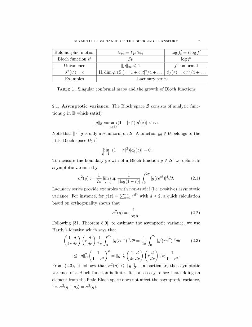
While the two approaches above for constructing flows of conformal maps
are somewhat different, there is a relation: singular quasicircles lead to
singular conformal maps via welding-type procedures [32]. The parallels
are summarised in Table 1 below, where exact equalities hold only in the
dynamical setting.
2. Bergman projection and Bloch functions
In this section, we introduce the notion of asymptotic variance for Bloch
functions and discuss some of its basic properties.
ASYMPTOTIC VARIANCE OF THE BEURLING TRANSFORM 7
Holomorphic motion ∂ϕt = t µ ∂ϕt log f ′t = t log f ′
Bloch function v′ Sµ log f ′
Univalence ‖µ‖∞ 6 1 f conformal
σ2(v′) = c H. dimϕt(S1) = 1 + c |t|2/4 + . . . βf (τ) = c τ2/4 + . . .
Examples Lacunary series
Table 1. Singular conformal maps and the growth of Bloch functions
2.1. Asymptotic variance. The Bloch space B consists of analytic func-
tions g in D which satisfy
‖g‖B := supz∈D
(1− |z|2)|g′(z)| <∞.
Note that ‖ · ‖B is only a seminorm on B. A function g0 ∈ B belongs to the
little Bloch space B0 if
lim|z|→1−
(1− |z|2)|g′0(z)| = 0.
To measure the boundary growth of a Bloch function g ∈ B, we define its
asymptotic variance by
σ2(g) :=1
2πlim supr→1−
1
| log(1− r)|
ˆ 2π
0|g(reiθ)|2dθ. (2.1)
Lacunary series provide examples with non-trivial (i.e. positive) asymptotic
variance. For instance, for g(z) =∑∞
n=1 zdn with d ≥ 2, a quick calculation
based on orthogonality shows that
σ2(g) =1
log d. (2.2)
Following [31, Theorem 8.9], to estimate the asymptotic variance, we use
Hardy’s identity which says that(1
4r
d
dr
)(rd
dr
)1
2π
ˆ 2π
0|g(reiθ)|2dθ =
1
2π
ˆ 2π
0|g′(reiθ)|2dθ (2.3)
≤ ‖g‖2B(
1
1− r2
)2
= ‖g‖2B(
1
4r
d
dr
)(rd
dr
)log
1
1− r2.
From (2.3), it follows that σ2(g) 6 ‖g‖2B. In particular, the asymptotic
variance of a Bloch function is finite. It is also easy to see that adding an
element from the little Bloch space does not affect the asymptotic variance,
i.e. σ2(g + g0) = σ2(g).
8 K. ASTALA, O. IVRII, A. PERALA, AND I. PRAUSE
2.2. Beurling transform and the Bergman projection. For a measur-
able function µ with |µ| 6 χD, the Beurling transform g = Sµ is an analytic
function in the exterior disk D∗ = z : |z| > 1 which satisfies a Bloch bound
of the form ‖g‖B∗ := |g′(z)|(|z|2−1) 6 C. Note that we use the notation B∗
for functions in D∗ – we reserve the symbol B for the standard Bloch space
in the unit disk D. By passing to the unit disk, we are naturally led to the
Bergman projection
Pµ(z) =1
π
ˆD
µ(w)dm(w)
(1− zw)2(2.4)
and its action on L∞-functions. Indeed, comparing (1.4) and (2.4), we see
that Pµ(1/z) = − z2Sµ0(z) for µ0(w) = µ(w) and z ∈ D∗. From this
connection between the Beurling transform and the Bergman projection, it
follows that
Σ2 = sup|µ|6χD
σ2(Sµ) = sup|µ|6χD
σ2(Pµ). (2.5)
In view of the above equation, the Beurling transform and the Bergman
projection are mostly interchangeable. Due to natural connections with
the quasiconformal literature, we mostly work with the Beurling transform.
However, in this section on a priori bounds, it is preferable to work with the
Bergman projection to keep the discussion in the disk.
2.3. Pointwise estimates. According to [29], the seminorm of the Bergman
projection from L∞(D)→ B is 8/π. Integrating (2.3), we get
1
2π
ˆ 2π
0|Pµ(reiθ)|2dθ ≤
(8
π
)2
log1
1− r2, r → 1−,
which implies that Σ2 6 (8/π)2. One can also equip the Bloch space with
seminorms that use higher order derivatives
‖f‖B,m = supz∈D
(1− |z|2)m|f (m)(z)|, (2.6)
where m > 1 is an integer. Very recently, Kalaj and Vujadinovic [16] cal-
culated the seminorm of the Bergman projection when the Bloch space is
equipped with (2.6). According to their result,
‖P‖B,m =Γ(2 +m)Γ(m)
Γ2(m/2 + 1). (2.7)
ASYMPTOTIC VARIANCE OF THE BEURLING TRANSFORM 9
It is possible to apply the differential operator in (2.3) m times and use the
pointwise estimates (2.7). In this way, one ends up with the upper bounds
σ2(Sµ) = σ2(Pµ) 6Γ(2 +m)2Γ(m)2
Γ(2m)Γ4(m/2 + 1). (2.8)
Putting m = 2 in (2.8), one obtains that σ2(Sµ) ≤ 6, which is a slight
improvement to (8/π)2 and is the best upper bound that can be achieved
with this argument. Using quasiconformal methods in Section 4, we will
show the significantly better upper bound σ2(Sµ) 6 1.
2.4. Cesaro integral averages. In Section 6 on fractal approximation,
we will need the Cesaro integral averages from [27, Section 6]. Following
McMullen, for f ∈ B, m > 1 and r ∈ [0, 1), we define
σ22m(f, r) =
1
Γ(2m)
1
| log(1− r)|
ˆ r
0
ds
1− s
[1
2π
ˆ 2π
0
∣∣∣∣(1− s2)mf (m)(seiθ)
∣∣∣∣2dθ]
and
σ22m(f) = lim sup
r→1−σ2
2m(f, r). (2.9)
We will need [27, Theorem 6.3] in a slightly more general form, where we
allow the use of “limsup” instead of requiring the existence of a limit:
Lemma 2.1. For f ∈ B,
σ2(f) = σ22(f) = σ2
4(f) = σ26(f) = . . . (2.10)
Furthermore, if the limit as r → 1 in σ22m(f) exists for some m > 0, then
the limit as r → 1 exists in σ22m(f) for all m > 0.
The original proof from [27] applies in this setting.
3. Holomorphic families
Our aim is to understand holomorphic families of conformal maps, and
the infinitesimal change of Hausdorff dimension. The natural setup for this
is provided by holomorphic motions [23], maps Φ : D×A→ C, with A ⊂ C,
such that
• For a fixed a ∈ A, the map λ→ Φ(λ, a) is holomorphic in D.
• For a fixed λ ∈ D, the map a→ Φ(λ, a) = Φλ(a) is injective.
• The mapping Φ0 is the identity on A,
Φ(0, a) = a, for every a ∈ A.
10 K. ASTALA, O. IVRII, A. PERALA, AND I. PRAUSE
It follows from the works of Mane-Sad-Sullivan [23] and Slodkowski [40]
that each Φλ can be extended to a quasiconformal homeomorphism of C.
In other words, each f = Φλ is a homeomorphic W 1,2loc (C)-solution to the
Beltrami equation
∂f(z) = µ(z)∂f(z) for a.e. z ∈ C.
Here the dilatation µ(z) = µλ(z) is measurable in z ∈ C, and the mapping
f is called k-quasiconformal if ‖µ‖∞ ≤ k < 1. As a function of λ ∈ D, the
dilatation µλ is a holomorphic L∞-valued function with ‖µλ‖∞ ≤ |λ|, see
[10]. In other words, Φλ is a |λ|-quasiconformal mapping.
Conversely, as is well-known, homeomorphic solutions to the Beltrami
equation can be embedded into holomorphic motions. For this work, we shall
need a specific and perhaps non-standard representation of the mappings
which quickly implies the embedding. For details, see Section 4.
3.1. Quasicircles. Let us now consider a holomorphic family of conformal
maps ϕt : D∗ → C, t ∈ D such as the one in the introduction. That is,
we assume ϕ(t, z) = ϕt(z) is a D × D∗ → C holomorphic motion which
in addition is conformal in the parameter z. By the previous discussion,
each ϕt extends to a |t|-quasiconformal mapping of C. Moreover, by sym-
metrising the Beltrami coefficients like in [18, 41], we see that ϕt(S1) is a
k-quasicircle, where |t| = 2k/(1 + k2). More precisely, ϕt(S1) = f(R ∪ ∞)for a k-quasiconformal map f : C → C of the Riemann sphere C, which is
antisymmetric with respect to the real line in the sense that
µf (z) = −µf (z) for a.e. z ∈ C.
Smirnov used this antisymmetric representation to prove (1.9). In terms of
the conformal maps ϕt, Smirnov’s result takes the form mentioned in (1.3).
3.2. Heuristics for σ2(Sµ) 6 1. An estimate based on the τ = 2 case of
[32, Theorem 3.3] tells us roughly that for R > 1,
1
2πR
ˆ|z|=R
|ϕ′t(z)|2|dz| 6 C(|t|) (R− 1)−|t|2. (3.1)
(The precise statement is somewhat weaker but we are not going to use this.)
A natural strategy for proving σ2(Sµ) 6 1 is to consider the holomorphic
ASYMPTOTIC VARIANCE OF THE BEURLING TRANSFORM 11
motion of principal mappings ϕt generated by µ,
∂ϕt = tµ ∂ϕt, t ∈ D; ϕt(z) = z +O(1/z) as z →∞.
For the derivatives, we have the Neumann series expansion:
ϕ′t = ∂ϕt = 1 + tSµ+ t2SµSµ+ . . . , z ∈ D∗. (3.2)
In view of this, taking the limit t→ 0 in (3.1), one obtains a growth bound
(as R → 1) for the integrals´|z|=R |Sµ|
2|dz|. However, in order to validate
this strategy, one needs to have good control on the constant term C(|t|)in (3.1). Namely, one would need to show that C(|t|) → 1 as t → 0 fast
enough, for instance at a quadratic rate C(|t|) 6 C |t|2 . Unfortunately, while
the growth exponent in (3.1) is effective, the constant is not.
In order to make this strategy work, we need two improvements. First, we
work with quasiconformal maps that are antisymmetric with respect to the
unit circle; and secondly, we use normalised solutions instead of principal
solutions. One of the key estimates will be Theorem 4.4 which is the coun-
terpart of (3.1) for antisymmetric maps, but crucially with a multiplicative
constant of the form C(δ)k2. This naturally complements the Hausdorff
measure estimates of [33].
3.3. Interpolation. Let (Ω, σ) be a measure space and Lp(Ω, σ) be the
usual spaces of complex-valued σ-measurable functions on Ω equipped with
the (quasi)norms
‖Φ‖p =
(ˆΩ|Φ(x)|p dσ(x)
) 1p
, 0 < p <∞.
In the papers [4] – [7], holomorphic deformations were used to give sharp
bounds on the distortion of quasiconformal mappings. In [6], the method
was formulated as a compact and general interpolation lemma:
Lemma 3.1. [6, Interpolation Lemma for the disk] Let 0 < p0, p1 6 ∞and Φλ ; |λ| < 1 ⊂ M (Ω, σ) be an analytic and non-vanishing family
of measurable functions defined on a domain Ω. Suppose
M0 := ‖Φ0‖p0 <∞, M1 := sup|λ|<1‖Φλ‖p1 <∞ and Mr := sup
|λ|=r‖Φλ‖pr ,
where1
pr=
1− r1 + r
· 1
p0+
2r
1 + r· 1
p1.
12 K. ASTALA, O. IVRII, A. PERALA, AND I. PRAUSE
Then, for every 0 6 r < 1 , we have
Mr 6 M1−r1+r
0 ·M2 r1+r
1 < ∞. (3.3)
To be precise, in the lemma we consider analytic families Φλ of measurable
functions in Ω, i.e. jointly measurable functions (x, λ) 7→ Φλ(x) defined on
Ω × D, for which there exists a set E ⊂ Ω of σ-measure zero such that for
all x ∈ Ω \ E, the map λ 7→ Φλ(x) is analytic and non-vanishing in D.
For the study of the asymptotic variance of the Beurling transform, we
need to combine interpolation with ideas from [41] to take into account the
antisymmetric dependence on λ, see Proposition 4.3. In this special setting,
Lemma 3.1 takes the following form:
Corollary 3.2. Suppose Φλ ; λ ∈ D is an analytic family of measurable
functions, such that for every λ ∈ D,
Φλ(x) 6= 0 and∣∣Φλ(x)
∣∣ =∣∣Φ−λ(x)
∣∣, for a.e. x ∈ Ω. (3.4)
Let 0 < p0, p1 6∞. Then, for all 0 6 k < 1 and exponents pk defined by
1
pk=
1− k2
1 + k2· 1
p0+
2k2
1 + k2· 1
p1,
we have
‖Φk‖pk 6 ‖Φ0‖1−k21+k2
p0
(sup|λ|<1‖Φλ‖p1
) 2k2
1+k2 ,
assuming that the right hand side is finite.
Proof. Consider the analytic family λ 7→√
Φλ(x) Φ−λ(x). The non-vanishing
condition ensures that we can take an analytic square-root. Since the depen-
dence with respect to λ gives an even analytic function, there is a (single-
valued) analytic family Ψλ such that
Ψλ2(x) =√
Φλ(x) Φ−λ(x).
Observe that |Φλ(x)| = |Ψλ2(x)| for real λ by the condition (3.4). By the
Cauchy-Schwarz inequality, Ψλ satisfies the same Lp1-bounds:
‖Ψλ2‖p1 ≤ ‖Φλ‖1/2p1 ‖Φ−λ‖1/2p1 ≤ sup|λ|<1‖Φλ‖p1 , λ ∈ D.
ASYMPTOTIC VARIANCE OF THE BEURLING TRANSFORM 13
We can now apply the Interpolation Lemma for the non-vanishing family
Ψλ with r = k2 to get
‖Φk‖pk = ‖Ψk2‖pk 6 ‖Ψ0‖1−k21+k2
p0
(sup|λ|<1‖Ψλ‖p1
) 2k2
1+k2
6 ‖Φ0‖1−k21+k2
p0
(sup|λ|<1‖Φλ‖p1
) 2k2
1+k2 .
4. Upper bounds
In this section, we apply quasiconformal methods for finding bounds on
integral means to the problem of maximising the asymptotic variance σ2(Sµ)
of the Beurling transform. Our aim is to establish the following result:
Theorem 4.1. Suppose µ is measurable with |µ| 6 χD. Then, for all 1 <
R < 2,
1
2π
ˆ 2π
0|Sµ(Reiθ)|2dθ ≤ (1 + δ) log
1
R− 1+ c(δ), 0 < δ < 1, (4.1)
where c(δ) <∞ is a constant depending only on δ.
The growth rate in (4.1) is interesting only for R close to 1: For |z| =
R > 1, we always have the pointwise bound
|Sµ(z)| =∣∣∣∣ 1π
ˆD
µ(ζ)
(ζ − z)2dm(ζ)
∣∣∣∣ ≤ 1
(R− 1)2. (4.2)
It is clear that Theorem 4.1 implies Σ2 6 1, i.e. the statement from Theorem
1.1 that
σ2(Sµ) =1
2πlim supR→1+
1
| log(R− 1)|
ˆ 2π
0|Sµ(Reiθ)|2 dθ 6 1 (4.3)
whenever |µ| 6 χD.
The proof of Theorem 4.1 is based on holomorphic motions and quasicon-
formal distortion estimates. In particular, we make strong use of the ideas
of Smirnov [41], where he showed that the dimension of a k-quasicircle is at
most 1 + k2. We first need a few preliminary results.
14 K. ASTALA, O. IVRII, A. PERALA, AND I. PRAUSE
4.1. Normalised solutions. The classical Cauchy transform of a function
ω ∈ Lp(C) is given by
Cω(z) =1
π
ˆC
ω(ζ)
z − ζdm(ζ). (4.4)
For us it will be convenient to use a modified version
C1ω(z) :=1
π
ˆCω(ζ)
[1
z − ζ− 1
1− ζ
]dm(ζ) (4.5)
= (1− z) 1
π
ˆCω(ζ)
1
(z − ζ)(1− ζ)dm(ζ)
defined pointwise for compactly supported functions ω ∈ Lp(C), p > 2. Like
the usual Cauchy transform, the modified Cauchy transform satisfies the
identities ∂(C1ω) = ω and ∂(C1ω) = Sω. Furthermore, C1ω is continuous,
vanishes at z = 1 and has the asymptotics
C1ω(z) = − 1
π
ˆC
ω(ζ)
1− ζdm(ζ) +O(1/z) as z →∞.
We will consider quasiconformal mappings with Beltrami coefficient µ
supported on unions of annuli
A(ρ,R) := z ∈ C : ρ < |z| < R.
Typically, we need to make sure that the support of the Beltrami coefficient
is symmetric with respect to the reflection in the unit circle. Therefore, it
is convenient to use the notation
AR := A(1/R,R), 1 < R <∞ and (4.6)
Aρ,R := A(1/R, 1/ρ) ∪A(ρ,R), 1 < ρ < R <∞. (4.7)
For coefficients supported on annuli AR, the normalised homeomorphic
solutions to the Beltrami equation
∂f(z) = µ(z)∂f(z) for a.e. z ∈ C, f(0) = 0, f(1) = 1, (4.8)
admit a simple representation:
Proposition 4.2. Suppose µ is supported on AR with ‖µ‖∞ < 1 and f ∈W 1,2loc (C) is the normalised homeomorphic solution to (4.8). Then
f(z) = z exp(C1ω(z)), z ∈ C, (4.9)
where ω ∈ Lp(C) for some p > 2, has support contained in AR and
ω(z)− µ(z)Sω(z) =µ(z)
zfor a.e. z ∈ C. (4.10)
ASYMPTOTIC VARIANCE OF THE BEURLING TRANSFORM 15
Proof. First, if ω satisfies the above equation, then
ω = (Id− µS)−1
(µ(z)
z
)=µ(z)
z+ µS
(µ(z)
z
)+ µSµS
(µ(z)
z
)+ · · ·
with the series converging in Lp(C) whenever ‖µ‖∞‖S‖Lp < 1, in particular
for some p > 2. The solution, unique in Lp(C), clearly has support contained
in AR.
If f(z) is as in (4.9), then f ∈W 1,2loc (C) and satisfies (4.8) with the required
normalisation. To see that f is a homeomorphism, note that
f(z) = α[z + β +O(1/z)] as z →∞, (4.11)
where
α = exp
(− 1
π
ˆC
ω(ζ)
1− ζdm(ζ)
)6= 0 and β =
1
π
ˆCω(ζ)dm(ζ) (4.12)
which shows that f is a composition of a similarity and a principal solution to
the Beltrami equation. Since every principal solution to a Beltrami equation
is automatically a homeomorphism [5, p.169], we see that f must be a
homeomorphism as well. The proposition now follows from the uniqueness
of normalised homeomorphic solutions to (4.8).
4.2. Antisymmetric mappings. If the Beltrami coefficient in (4.8) sat-
isfies µ(z) = µ(z), then by the uniqueness of the normalised solutions, we
have f(z) = f(z) and f preserves the real axis.
For normalised solutions preserving the unit circle, the corresponding con-
dition for f is f(1/z) = 1/f(z) which asks for the Beltrami coefficient to
satisfy µ( 1z ) z
2
z2= µ(z) for a.e. z ∈ C. In this case, we say that the Beltrami
coefficient µ is symmetric (with respect to the unit circle). Following [41],
we say that µ is antisymmetric if
µ
(1
z
)z2
z2= −µ(z) for a.e. z ∈ C. (4.13)
Given an antisymmetric µ supported on AR with ‖µ‖∞ = 1, define
µλ(z) = λµ(z), λ ∈ D,
and let fλ be the corresponding normalised homeomorphic solution to (4.8)
with µ = µλ. It turns out that in case of mappings antisymmetric with
16 K. ASTALA, O. IVRII, A. PERALA, AND I. PRAUSE
respect to the circle, the expression
Φλ(z) := z∂fλ(z)
fλ(z)
has the proper invariance properties similar to those used in [41]:
Proposition 4.3. For every λ ∈ D and z ∈ C,
1
z
∂fλ(1/z)
fλ(1/z)=
[z∂f(−λ )(z)
f(−λ )(z)
].
In particular, ∣∣∣∣ ∂fλ(z)
fλ(z)
∣∣∣∣ =
∣∣∣∣∣ ∂f(−λ )(z)
f(−λ )(z)
∣∣∣∣∣ whenever |z| = 1.
Proof. Let
gλ(z) =1
fλ(1/z), z ∈ C. (4.14)
By direct calculation, gλ has complex dilatation λµ( 1z ) z
2
z2which by our
assumption on antisymmetry is equal to −λµ(z). Since gλ and f−λ are
normalised solutions to the same Beltrami equation, the functions must be
identical. Differentiating the identity (4.14) with respect to ∂/∂z, we get
∂f(−λ)(z) =1
z2
∂fλ(1/z)
fλ(1/z)2= f(−λ)(z)
1
z2
∂fλ(1/z)
fλ(1/z).
Rearranging and taking the complex conjugate gives the claim.
4.3. Integral means for antisymmetric mappings. For 1 < R < 2,
consider a quasiconformal mapping f whose Beltrami coefficient is supported
on AR,2. Since f is conformal in the narrow annulus 1R < |z| < R, it is
reasonable to study bounds for the integral means involving the derivatives
of f on the unit circle. We are especially interested in the dependence of
these bounds on R as R→ 1+.
Theorem 4.4. Suppose µ is measurable, |µ(z)| ≤ (1− δ)χAR,2(z), and that
µ is antisymmetric. Let 0 ≤ k ≤ 1.
If f = fk ∈W 1,2loc (C) is the normalised homeomorphic solution to ∂f(z) =
kµ(z)∂f(z), then
1
2π
ˆ|z|=1
∣∣∣∣ f ′(z)f(z)
∣∣∣∣2 |dz| ≤ C(δ)k2
(R− 1)− 2k2
1+k2 , (4.15)
where C(δ) <∞ is a constant depending only on δ.
ASYMPTOTIC VARIANCE OF THE BEURLING TRANSFORM 17
The assumption ‖µ(z)‖∞ ≤ 1−δ above, where δ > 0 is fixed but arbitrary,
is made to guarantee that we have uniform bounds in (4.15) for all k < 1. To
estimate the asymptotic variance of the Beurling transform, we will study
the nature of these bounds as k → 0, but we need to keep in mind the
dependence on the auxiliary parameter δ > 0.
Proof of Theorem 4.4. We embed f in a holomorphic motion by setting
µλ(z) = λ µ(z), λ ∈ D.
Let fλ denote the normalised solution to the Beltrami equation fz = µλfz,
with the representation (4.9) described in Proposition 4.2. The uniqueness
of the solution implies that fk = f .
We now apply Corollary 3.2 to the family
Φλ(z) := z(fλ)′(z)
fλ(z), λ ∈ D, z ∈ S1. (4.16)
By [5, Theorem 5.7.2], the map is well-defined, nonzero and holomorphic
in λ for each z ∈ S1. By the antisymmetry of the dilatation µ, we can use
Proposition 4.3 to get the identity
∣∣Φλ(z)∣∣ =
∣∣∣∣ ∂fλ(z)
fλ(z)
∣∣∣∣ =
∣∣∣∣∣ ∂f(−λ )(z)
f(−λ )(z)
∣∣∣∣∣ =∣∣Φ−λ(z)
∣∣, z ∈ S1. (4.17)
We first find a global L2-bound, independent of λ ∈ D. For this purpose,
we estimate
1
2π
ˆAR
∣∣∣∣ f ′λ(z)
fλ(z)
∣∣∣∣2 dm(z).
Recall that 1 < R < 2 by assumption. Since all fλ’s are normalised 1+δ1−δ -
quasiconformal mappings, we have
|fλ(z)| = |fλ(z)− fλ(0)||fλ(1)− fλ(0)|
≥ 1/ρδ, 1/R < |z| < R,
together with
fλ(AR) ⊂ fλB(0, 2) ⊂ B(0, ρδ).
Therefore,
1
2π
ˆAR
∣∣∣∣ f ′λ(z)
fλ(z)
∣∣∣∣2 dm(z) ≤ 1
2πρ2δ |fλAR| ≤ ρ4
δ/2 (4.18)
18 K. ASTALA, O. IVRII, A. PERALA, AND I. PRAUSE
for some constant 1 < ρδ <∞ depending only on δ. In particular,
(R− 1)1
2π
ˆ|z|=1
∣∣∣∣ f ′λ(z)
fλ(z)
∣∣∣∣2 |dz| 6 c(δ) <∞, λ ∈ D,
where the bound c(δ) depends only on 0 < δ < 1.
We now use interpolation to improve the L2-bounds near the origin. We
choose p0 = p1 = 2, Ω = S1 and dσ(z) = R−12π |dz|. Applying Corollary 3.2
gives
(R− 1)1
2π
ˆ|z|=1
∣∣∣∣ f ′k(z)fk(z)
∣∣∣∣2 |dz| 6 (R− 1)1−k21+k2 c(δ)
2k2
1+k2 ,
which implies Theorem 4.4.
4.4. Integral means for the Beurling transform. We now use infinites-
imal estimates for quasiconformal distortion to give bounds for the integral
means of Sµ. We begin with the following lemma:
Lemma 4.5. Given 1 < R < 2, suppose µ is an antisymmetric Beltrami
coefficient with suppµ ⊂ AR,2 and ‖µ‖∞ 6 1. Then, µ1(z) := µ(z)z satisfies
1
2π
ˆ|z|=1
|Sµ1(z)|2|dz| ≤ (1 + δ) log1
(R− 1)2+ logC(δ/4), 0 < δ < 1,
where C(δ) is the constant from Theorem 4.4.
Proof. First, observe that if h is any L1-function vanishing in the annulus
z : 1/R < |z| < R, by the theorems of Fubini and Cauchy,
1
2π
ˆ|z|=1
z(Sh)(z) |dz| =1
2πi
ˆS1
(Sh)(z)dz
=1
π
ˆCh(ζ)
[1
2πi
ˆS1
1
(ζ − z)2dz
]dm(ζ) = 0.
To apply Theorem 4.4, take 0 < k < 1 and solve the Beltrami equation
∂f(z) = kν(z)∂f(z) for the coefficient ν(z) = (1− δ)µ(z). Let fk ∈W 1,2loc (C)
be the normalised homeomorphic solution in C.
Recall from (4.9) that fk has the representation fk(z) = z exp(C1ω(z))
where
ω = (Id− k νS)−1
(k ν(z)
z
)= k(1− δ)µ1(z) + k2(1− δ)2 νSµ1(z) + · · ·
and the series converges in Lp(C) for some fixed p = p(δ) > 2. From this
representation, we see that
zf ′k(z)
fk(z)= 1 + k(1− δ)zSµ1(z) + k2(1− δ)2zSνSµ1(z) +O(k3) (4.19)
ASYMPTOTIC VARIANCE OF THE BEURLING TRANSFORM 19
holds pointwise in the annulus z : 1/R < |z| < R, where ν and ω vanish.
It follows that
1
2π
ˆ|z|=1
∣∣∣∣f ′k(z)fk(z)
∣∣∣∣2 |dz| = 1+k2(1−δ)2 1
2π
ˆ|z|=1
|Sµ1(z)|2|dz|+O(k3). (4.20)
Finally, combining (4.20) with Theorem 4.4, we obtain
1 + k2(1− δ)2 1
2π
ˆ|z|=1
|Sµ1(z)|2|dz|+O(k3)
≤ exp
(k2 logC(δ) +
k2
1 + k2log
1
(R− 1)2
)= 1 + k2 logC(δ) + k2 log
1
(R− 1)2+O(k4).
Taking k → 0, we find that
1
2π
ˆ|z|=1
|Sµ1(z)|2|dz| ≤ (1− δ)−2 log1
(R− 1)2+ (1− δ)−2 logC(δ).
As (1− δ/4)−2 ≤ 1 + δ, replacing δ by δ/4 proves the lemma.
Corollary 4.6. Given 1 < R < 2, suppose µ is a Beltrami coefficient with
suppµ ⊂ A(1/2, 1/R) and ‖µ‖∞ ≤ 1. Then,
1
2π
ˆ|z|=1
|Sµ(z)|2|dz| ≤ (1 + δ) log1
(R− 1)+
1
2logC(δ/4), 0 < δ < 1,
where C(δ) is the constant from Theorem 4.4.
Proof. Define an auxiliary Beltrami coefficient ν by requiring ν(z) = zµ(z)
for |z| ≤ 1 and ν(z) = − z2
z2ν(1/z) for |z| ≥ 1. Then ν is supported on AR,2,
‖ν‖∞ ≤ 1 and ν is antisymmetric, so that with help of Lemma 4.5 we can
estimate the integral means of Sν1, where ν1(z) = ν(z)z .
On the other hand, the antisymmetry condition (4.13) implies
C(χDν1)(1/z) = C(χC\Dν1)(z) − C(χC\Dν1)(0)
for the Cauchy transform. Differentiating this with respect to ∂/∂z gives
1
zS(χDν1)
(1
z
)= − zS(χC\Dν1)(z).
In particular, for z on the unit circle S1,
zS(ν1)(z) = zS(χDν1)(z) + zS(χC\Dν1)(z)
= 2i Im[z S(χDν1)(z)
]= 2i Im
[z (Sµ)(z)
].
20 K. ASTALA, O. IVRII, A. PERALA, AND I. PRAUSE
In other words, the estimates of Lemma 4.5 take the form
1
2π
ˆ|z|=1
∣∣∣Im[z (Sµ)(z)]∣∣∣2|dz| = 1
4
1
2π
ˆ|z|=1
|Sν1(z)|2|dz|
≤ 1
4(1 + δ) log
1
(R− 1)2+
1
4logC(δ/4), 0 < δ < 1.
By replacing µ with iµ, we see that the same bound holds for the integral
means of Re[z (Sµ)(z)]. Therefore,
1
2π
ˆ|z|=1
|Sµ(z)|2|dz| =1
2π
ˆ|z|=1
∣∣∣Re[z (Sµ)(z)
]∣∣∣2 +∣∣∣Im[z (Sµ)(z)
]∣∣∣2 |dz|≤ (1 + δ) log
1
R− 1+
1
2logC(δ/4)
for every 0 < δ < 1.
4.5. Asymptotic variance. With these preparations, we are ready to prove
Theorem 4.1. We need to show that if µ is measurable with |µ(z)| ≤ χD,
then for all 1 < R < 2,
1
2π
ˆ 2π
0|Sµ(Reiθ)|2dθ ≤ (1 + δ) log
1
R− 1+ c(δ), 0 < δ < 1,
where c(δ) <∞ is a constant depending only on δ.
Proof of Theorem 4.1. For a proof of this inequality, first assume that addi-
tionally
µ(z) = 0 for |z| < 3/4; 1 < R <3
2. (4.21)
Then ν(z) := µ(Rz) has support contained in B(0, 1/R) \B(0, 1/2) so that
we may apply Corollary 4.6. Since Sν(z) = Sµ(Rz),
1
2π
ˆ 2π
0|Sµ(Reiθ)|2dθ =
1
2π
ˆ|z|=1
|Sν(z)|2|dz|
≤ (1 + δ) log1
R− 1+
1
2logC(δ/4),
which is the desired estimate.
For the general case when (4.21) does not hold, write µ = µ1 + µ2 where
µ2(z) = χB(0,3/4)µ(z). As
|Sµ2(z)| ≤ˆ
14<|z−ζ|<2
1
|ζ − z|2dm(ζ) = 2π log(8), |z| = 1,
we have1
2π
ˆ 2π
0|Sµ1(Reiθ) + Sµ2(Reiθ)|2dθ
ASYMPTOTIC VARIANCE OF THE BEURLING TRANSFORM 21
≤ (1 + δ)1
2π
ˆ 2π
0|Sµ1(Reiθ)|2dθ +
(1 +
1
δ
)1
2π
ˆ 2π
0|Sµ2(Reiθ)|2dθ
≤ (1 + δ)2 log1
R− 1+
1 + δ
2logC(δ/4) +
1 + δ
δ4π2 log2(8)
for 0 < δ < 1 and 1 < R < 32 ; while for R > 3
2 , we have the pointwise bound
(4.2). Finally, replacing δ by δ/3, we get the estimate in the required form,
thus proving the theorem.
5. Lower bounds
Consider the family of polynomials
Pt(z) = zd + t z, |t| < 1,
for d > 2. According to [27, Theorem 1.8] or [1, 39], the Hausdorff dimen-
sions of their Julia sets satisfy
H.dim J (Pt) = 1 +|t|2(d− 1)2
4d2 log d+O(|t|3). (5.1)
Moreover, each Julia set J (Pt) is a quasicircle, the image of the unit circle
by a quasiconformal mapping of the plane. A quick way to see this is to
observe that the immediate basin of attraction of the origin contains all
the (finite) critical points of Pt. (From general principles, it is clear that
the basin must contain at least one critical point, but by the (d − 1)-fold
symmetry of Pt, it must contain them all.)
If APt(∞) denotes the basin of attraction of infinity, for each |t| < 1 there
is a canonical conformal mapping
ϕt : D∗ = AP0(∞)→ APt(∞) (5.2)
conjugating the dynamics:
ϕt P0(z) = Pt ϕt(z), z ∈ D∗. (5.3)
By Slodkowski’s extended λ-lemma [40] and the properties of holomorphic
motions, ϕt extends to a |t|-quasiconformal mapping of the plane, see e.g. [5,
Section 12.3]. In particular, the extension maps the unit circle onto the Julia
set J (Pt).
22 K. ASTALA, O. IVRII, A. PERALA, AND I. PRAUSE
While the extensions given by the λ-lemma are natural, surprisingly it
turns out that the maps ϕt have extensions with considerably smaller qua-
siconformal distortion, smaller by a factor of
cd :=d
1d−1
2, 2 ≤ d ∈ N, (5.4)
when |t| → 0.
Theorem 5.1. Let Pt(z) = zd + tz with |t| < 1. Then the canonical conju-
gacy ϕt : D∗ → APt(∞), defined in (5.2), has a µt-quasiconformal extension
with
‖µt‖∞ = cd|t|+O(|t|2).
Here c2 = 1, but cd < 1 for d > 3. Hence for every degree > 3 we
have an improved bound for the distortion. Furthermore, when representing
J (Pt) as the image of the unit circle by a map with as small distortion
as possible, one can apply Theorem 5.1 together with the symmetrisation
method described in Section 3.1 to show that each J (Pt) is a k(t)-quasicircle,
where
k(t) =cd2|t|+O(|t|2).
By the dimension formula (5.1),
H. dim J (Pt) = 1 +4d
21−d (d− 1)2
d2 log d|k(t)|2 +O(|k(t)|3). (5.5)
In particular, when d = 20, we get k-quasicircles whose Hausdorff dimension
is greater than 1 + 0.87913 k2, for small values of k. Therefore, Theorem 1.3
follows from Theorem 5.1.
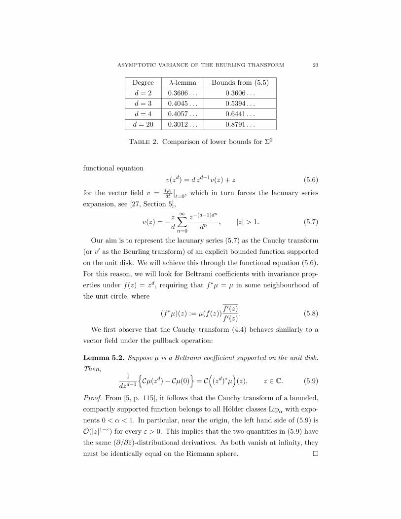
The numerical values for the second order term of (5.5) are presented in
Table 2 below. These provide lower bounds on the asymptotic variance (or
equivalently, on the quasicircle dimension asymptotics). For comparison, we
also show the values for the second order term of (5.1) which correspond to
the estimate on quasiconformal distortion provided by the λ-lemma. Note
that the first explicit lower bound on quasicircle dimension asymptotics [9]
is exactly the degree 2 case of the upper-left corner.
For the proof of Theorem 5.1, we find an improved representation for the
infinitesimal vector field determined by ϕt. Differentiating (5.3), we get a
ASYMPTOTIC VARIANCE OF THE BEURLING TRANSFORM 23
Degree λ-lemma Bounds from (5.5)
d = 2 0.3606 . . . 0.3606 . . .
d = 3 0.4045 . . . 0.5394 . . .
d = 4 0.4057 . . . 0.6441 . . .
d = 20 0.3012 . . . 0.8791 . . .
Table 2. Comparison of lower bounds for Σ2
functional equation
v(zd) = d zd−1v(z) + z (5.6)
for the vector field v = dϕtdt
∣∣t=0
, which in turn forces the lacunary series
expansion, see [27, Section 5],
v(z) = −zd
∞∑n=0
z−(d−1)dn
dn, |z| > 1. (5.7)
Our aim is to represent the lacunary series (5.7) as the Cauchy transform
(or v′ as the Beurling transform) of an explicit bounded function supported
on the unit disk. We will achieve this through the functional equation (5.6).
For this reason, we will look for Beltrami coefficients with invariance prop-
erties under f(z) = zd, requiring that f∗µ = µ in some neighbourhood of
the unit circle, where
(f∗µ)(z) := µ(f(z))f ′(z)
f ′(z). (5.8)
We first observe that the Cauchy transform (4.4) behaves similarly to a
vector field under the pullback operation:
Lemma 5.2. Suppose µ is a Beltrami coefficient supported on the unit disk.
Then,1
dzd−1
Cµ(zd)− Cµ(0)
= C
((zd)∗µ
)(z), z ∈ C. (5.9)
Proof. From [5, p. 115], it follows that the Cauchy transform of a bounded,
compactly supported function belongs to all Holder classes Lipα with expo-
nents 0 < α < 1. In particular, near the origin, the left hand side of (5.9) is
O(|z|1−ε) for every ε > 0. This implies that the two quantities in (5.9) have
the same (∂/∂z)-distributional derivatives. As both vanish at infinity, they
must be identically equal on the Riemann sphere.
24 K. ASTALA, O. IVRII, A. PERALA, AND I. PRAUSE
Remark 5.3. Since the left hand side in (5.9) vanishes at 0, we always have
C((zd)∗µ
)(0) = 0. This can also be seen by using the change of variables
z → ζ · z where ζ is a d-th root of unity.
We will use the following basic Beltrami coefficients as building blocks:
Lemma 5.4. Let µn(z) :=(z/|z|
)n−2χA(r,ρ) with 0 < r < ρ < 1 and
2 6 n ∈ N. Then
Cµn(z) =2
n(ρn − rn) z−(n−1), |z| > 1,
and Cµn(0) = 0.
Proof. We compute:ˆDµn(w) · wn−2dm(w) =
ˆA(r,ρ)
|w|n−2dm(w) =2π
n(ρn − rn).
Hence, by orthogonality
Cµn(z) =1
πz
ˆD
µn(w)dm(w)
(1− w/z)
=1
πz
∞∑j=0
z−jˆDµn(w)wjdm(w)
=1
πz· z−(n−2) · 2π
n· (ρn − rn)
=2
n· z−(n−1) · (ρn − rn)
as desired. The claim Cµn(0) = 0 follows similarly.
To represent power series in z−1, we sum up µn’s supported on disjoint
annuli:
Lemma 5.5. For d > 3 and ρ0 ∈ (0, 1), let
nj = (d− 1) dj , rj = ρ1/nj0 , j = 0, 1, 2, . . .
and define the Beltrami coefficient µ by
µ(z) =(z/|z|
)nj−2, rj < |z| < rj+1, j ∈ N,
while for |z| < ρ1/n0
0 and for |z| > 1, we set µ(z) = 0. With these choices,
(i) µ = (zd)∗µ+ µ · χA(r0,r1) and
(ii) Cµ(zd) = dzd−1 Cµ(z)− 2dd−1 [ρ
1/d0 − ρ0] · z, |z| > 1.
In particular, for |z| > 1 we have
ASYMPTOTIC VARIANCE OF THE BEURLING TRANSFORM 25
(iii) Cµ(z) = − 2dd−1 [ρ
1/d0 − ρ0] v(z), with
(iv) Sµ(z) = − 2dd−1 [ρ
1/d0 − ρ0] v′(z),
where v = vd is the lacunary series in (5.7).
Proof. Claim (i) is clear from the construction. Inserting (i) into (5.9) and
using Lemma 5.4 gives (ii). This agrees with the functional equation (5.6)
up to a constant term in front of z which leads to (iii). Finally, (iv) follows
by differentiation.
Remark 5.6. The d = 2 case of Lemma 5.5 is somewhat different since the
vector field v2 does not vanish at infinity, so v2 is not the Cauchy transform
of any Beltrami coefficient. With the choice nj = 2j+1, (ii) and (iii) hold up
to an additive constant, while (iv) holds true as stated.
Differentiating (5.7), we see that
v′(z) =∑n>0
z−(d−1)dn · (d− 1)dn − 1
dn+1
=(d− 1)
d·∑n>0
z−(d−1)dn + b0
for some function b0 ∈ B∗0, which implies
σ2(v′(z)) =(d− 1)2
d2 log d.
Therefore, the Beltrami coefficient µ = µd from Lemma 5.5 satisfies
σ2(Sµ) =4[ρ
1/d0 − ρ0]2
log d.
Fixing d and optimising over ρ0 ∈ (0, 1), simple calculus reveals that the
maximum is obtained when ρ0 = dd
1−d . For this choice of ρ0,
v′(z) = −cd Sµ(z) (5.10)
where cd is the constant from (5.4). Moreover,
σ2(Sµ) = 4d2
1−d(d− 1)2
d2 log d(5.11)
obtains its maximum (over the natural numbers) at d = 20, in which case
σ2(Sµ20) > 0.87913, with |µ| = χD.
26 K. ASTALA, O. IVRII, A. PERALA, AND I. PRAUSE
This construction proves Theorem 1.2. One can proceed further from these
infinitesimal bounds and use (5.10) to produce quasicircles with large di-
mension. This takes us to Theorem 5.1.
Proof of Theorem 5.1. By the extended λ-lemma, the conformal maps
ϕt : D∗ → APt(∞),
admit quasiconformal extensionsHt : C→ C, which depend holomorphically
on t ∈ D. Since the Beltrami coefficient µHt is a holomorphic L∞-valued
function of t, the vector-valued Schwarz lemma implies that
µHt = tµ0 +O(t2)
for some Beltrami coefficient |µ0| ≤ χD. By developing ϕ′t = ∂zHt as a
Neumann series in SµHt , c.f. (3.2), we get
Sµ0(z) = v′(z), z ∈ D∗,
for the infinitesimal vector field v = dϕtdt
∣∣t=0
.
On the other hand, if µd is the Beltrami coefficient from Lemma 5.5, it
follows from (5.10) that µ#d := −cd µd also satisfies Sµ#
d (z) = v′(z) in D∗.Then the Beltrami coefficient µ0 − µ#
d is infinitesimally trivial, and by [20,
Lemma V.7.1], we can find quasiconformal maps Nt which are the identity
on the exterior unit disk and have dilatations µNt = t(µ0 − µ#d ) + O(t2),
|t| < 1. Therefore, we can replace Ht with Ht N−1t to obtain an extension
of ϕt with dilatation
µHtN−1t
= tµ#d +O(t2) (5.12)
as desired. This concludes the proof.
Remark 5.7. (i) One can show that for d > 2, the Beltrami coefficient µ#d
constructed in Lemma 5.5 is not infinitesimally extremal which implies that
the conformal maps ϕt (with t close to 0) admit even more efficient exten-
sions (i.e. with smaller dilatations). One reason to suspect that this may be
the case is that µ#d is not of the form q
|q| for some holomorphic quadratic
differential q on the unit disk; however, this fact alone is insufficient. It
would be interesting to find the dilatation of the most efficient extension,
but this may be a difficult problem. For more on Teichmuller extremality,
we refer the reader to the survey of Reich [38].
ASYMPTOTIC VARIANCE OF THE BEURLING TRANSFORM 27
(ii) Let Mshell be the class of Beltrami coefficients of the form
∞∑j=0
(z
|z|
)nj−2
· χA(ri,ri+1), 0 6 r0 < r1 < r2 < · · · < 1.
One can show that
Σ2 > supµ∈Mshell
σ2(Sµ) = maxd>1
4d2
1−d(d− 1)2
d2 log d≈ 0.87914
where the maximum is taken over all real d > 1.
6. Fractal approximation
In this section, we present an alternative route to the upper bound for the
asymptotic variance of the Beurling transform using (infinitesimal) fractal
approximation. We show that in order to compute Σ2 = sup|µ|6χD σ2(Sµ),
it suffices to take the supremum only over certain classes of “dynamical”
Beltrami coefficients µ for which McMullen’s formula holds, i.e.
2d2
dt2
∣∣∣∣t=0
H. dimϕt(S1) = limR→1+
1
2π| log(R− 1)|
ˆ 2π
0|v′µ(Reiθ)|2dθ (6.1)
where ϕt is the unique principal homeomorphic solution to the Beltrami
equation ∂ϕt = tµ ∂ϕt and vµ := dϕtdt
∣∣t=0
is the associated vector field. By
using the principal solution, we guarantee that vµ vanishes at infinity which
implies that vµ = Cµ. We will use this identity repeatedly. (In general,
when ϕt does not necessarily fix ∞, vµ and Cµ may differ by a quadratic
polynomial Az2 +Bz + C.)
Consider the following classes of dynamical Beltrami coefficients, with
each subsequent class being a subclass of the previous one:
• MB =⋃f Mf (D) consists of Beltrami coefficients that are eventually-
invariant under some finite Blaschke product f(z) = z∏d−1i=1
z−ai1−aiz ,
i.e. Beltrami coefficients which satisfy f∗µ = µ in some open neigh-
bourhood of the unit circle.
• MI =⋃d>2MI(d) consists of Beltrami coefficients that are eventually-
invariant under z → zd for some d > 2.
• MPP =⋃d>2MPP(d) consists of µ ∈ MI for which vµ arises as the
vector field associated to some polynomial perturbation of z → zd,
again for some d > 2. For details, see Section 6.3.
28 K. ASTALA, O. IVRII, A. PERALA, AND I. PRAUSE
Theorem 6.1. [27] If µ belongs to MB, then the function t→ H.dimϕt(S1)
is real-analytic and (6.1) holds.
While McMullen did not explicitly state the relation between Hausdorff
dimension and asymptotic variance for MB, the argument in [27] does apply
to conjugacies ϕt induced by this class of coefficients. Note that the class of
polynomial perturbations is explicitly covered in McMullen’s work, see [27,
Section 5]. We show:
Theorem 6.2.
Σ2 = supµ∈MI, |µ|6χD
σ2(Sµ) = supµ∈MPP, |µ|6χD
σ2(Sµ).
In view of Theorem 6.1, the first equality in Theorem 6.2 is sufficient to
deduce Theorem 1.4. With a bit more work, the second equality also gives
the following consequence:
Corollary 6.3. For any ε > 0, there exists a family of polynomials
zd + t(ad−2zd−2 + ad−3z
d−3 + · · ·+ a0), t ∈ (−ε0, ε0),
such that each Julia set Jt is a k(t)-quasicircle with
H. dim(Jt) > 1 + (Σ2 − ε)k(t)2.
6.1. Bounds on quadratic differentials. To prove Theorem 6.2, we work
with the integral average σ24 rather than with σ2. The reason for shifting
the point of view is due to the fact that the pointwise estimates for
v′′′µ (z) = − 6
π
ˆD
µ(w)
(w − z)4dm(w) (6.2)
are more useful than the pointwise estimates for v′, as we saw in Section 2
when we invoked Hardy’s identity. According to Lemma 2.1,
σ2(v′µ) = σ24(v′µ) =
8
3lim supR→1+
A(R,2)
∣∣∣∣v′′′µρ2∗
(z)
∣∣∣∣2 ρ∗(z)dm (6.3)
where ρ∗(z) = 2/(|z|2− 1) is the density of the hyperbolic metric on D∗ andfflf(z) ρ∗(z)dm denotes the integral average with respect to the measure
ρ∗(z)dm. (Note that we are not taking the average with respect to the
hyperbolic area ρ2∗(z)dm.)
We will need two estimates for v′′′/ρ2∗. To state these estimates, we in-
troduce some notation. For a set E ⊂ C, let E∗ denote its reflection in
ASYMPTOTIC VARIANCE OF THE BEURLING TRANSFORM 29
the unit circle. The hyperbolic distance between z1, z2 ∈ D∗ is denoted by
dD∗(z1, z2). The following lemma is based on ideas from [25, Section 2] and
appears explicitly in [15, Section 2]:
Lemma 6.4. Suppose µ is a measurable Beltrami coefficient with |µ| 6 χD
and v′′′ is given by (6.2). Then,
(a) |v′′′/ρ2∗| 6 3/2 for z ∈ D∗.
(b) If dD∗(z, supp(µ)∗) > L, then |(v′′′/ρ2∗)(z)| 6 Ce−L, for some con-
stant C > 0.
Proof. A simple computation shows that if γ is a Mobius transformation,
thenγ′(z1)γ′(z2)
(γ(z1)− γ(z2))2=
1
(z1 − z2)2, for z1 6= z2 ∈ C. (6.4)
The above identity and a change of variables shows that
v′′′µ (γ(z)) · γ′(z)2 = v′′′γ∗µ(z), (6.5)
analogous to the transformation rule of a quadratic differential.
In view of the Mobius invariance, it suffices to prove the assertions of the
lemma at infinity. From (6.2), one has
limz→∞
∣∣∣∣v′′′µρ2∗
(z)
∣∣∣∣ =3
2π
∣∣∣∣ˆDµ(w)dm(w)
∣∣∣∣ ,which gives (a). For (b), recall that dD∗(∞, z) = − log(|z| − 1) + O(1) for
|z| < 2. Then,
limz→∞
∣∣∣∣v′′′µρ2∗
(z)
∣∣∣∣ 6 3
2π
ˆ1−Ce−L<|w|<1
dm(w) = O(e−L)
as desired.
Remark 6.5. Loosely speaking, part (b) of Lemma 6.4 says that to determine
the value of v′′′µ /ρ2∗ at a point z ∈ D∗, one needs to know the values of µ in a
neighbourhood of z∗. More precisely, for any ε > 0, one may choose L > 0
sufficiently large to ensure that the contribution of the values of µ outside
w : dD(z∗, w) < L to (v′′′µ /ρ2∗)(z) is less than ε. In particular, if µ1 and
µ2 are two Beltrami coefficients, supported on the unit disk and bounded
by 1 that agree on w : dD(z∗, w) < L, then∣∣(v′′′µ1/ρ2
∗)(z)− (v′′′µ2/ρ2∗)(z)
∣∣ <2ε. This simple localisation principle will serve as the foundation for the
arguments in this section.
30 K. ASTALA, O. IVRII, A. PERALA, AND I. PRAUSE
Lemma 6.6. Given an ε > 0, there exists an 1 < R(ε) < ∞, so that if
1 < |z|d < R(ε), then ∣∣∣∣z2v′′′
(zd)∗µ
ρ2∗
(z)− z2dv′′′µρ2∗
(zd)
∣∣∣∣ < ε. (6.6)
Note that R(ε) is independent of the degree d > 2.
Proof. Differentiating (5.9) three times yields∣∣∣d2z2d−2v′′′µ (zd)− v′′′(zd)∗µ(z)∣∣∣ 6 2d2|z|−2ω(zd),
where ω(z)/ρ2∗(z) → 0 as |z| → 1+. The lemma follows in view of the
convergence (1/d) · (ρ∗(z)/ρ∗(zd)) → 1 as |z|d → 1+, which is uniform over
d > 2.
Alternatively, one can use a version of Koebe’s distortion theorem for
maps which preserve the unit circle, see [15, Section 2].
6.2. Periodising Beltrami coefficents. We now prove the first equality
in Theorem 6.2 which says that Σ2 = supµ∈MI, |µ|6χD σ2(Sµ). In view of
Lemma 2.1, given a Beltrami coefficient µ with |µ| 6 χD and ε > 0, it
suffices to construct an eventually-invariant Beltrami coefficient µd which
satisfies
|µd| 6 χD and σ24(v′µd) > σ
24(v′µ)− ε. (6.7)
Proof of Theorem 6.2, first equality. Given an integer d > 2, we construct a
Beltrami coefficient µd ∈ MI(d). We then show that µd satisfies (6.7) for d
sufficiently large.
Step 1. Using the definition of asymptotic variance (6.3), we select an
annulus
A∗0 = A(R1, R0) ⊂ D∗, R1 = R1/d0 , R0 ≈ 1,
for which
σ24(v′µ)− ε/3 6 8
3
A∗0
∣∣∣∣v′′′µρ2∗
(z)
∣∣∣∣2ρ∗(z)dm.Let A0 = A(r0, r1) be the reflection of A∗0 in the unit circle. We take µd = µ
on A0 and then extend µd to z : r1 < |z| < 1 by zd-invariance. On |z| < r0,
we set µd = 0.
ASYMPTOTIC VARIANCE OF THE BEURLING TRANSFORM 31
Step 2. The estimate (6.7) relies on an isoperimetric feature of the measure
ρ∗(z)dm, which we now describe. It is easy to see that the ρ∗(z)dm-area of
an annulus
A(S1, S2), 1 < S1 < S2 <∞,
is 2π times the hyperbolic distance between its boundary components. In
particular, the ρ∗(z)dm-area of A∗0 is roughly 2π log d. By contrast, for a
fixed L > 0, the ρ∗(z)dm-area of its “periphery”
∂LA∗0 := z ∈ A∗0, dD(z, ∂A∗0) < L
is 4πL (provided that log d > 2L). We conclude that the ratio of ρ∗(z)dm-
areas of ∂LA∗0 and A∗0 tends to 0 as d→∞.
Step 3. By part (b) of Lemma 6.4,∣∣∣∣v′′′µdρ2∗
(z)−v′′′µρ2∗
(z)
∣∣∣∣ 6 Ce−L, z ∈ A∗0 \ ∂LA∗0, (6.8)
while ∣∣∣∣v′′′µdρ2∗
(z)−v′′′µρ2∗
(z)
∣∣∣∣ 6 3, z ∈ ∂LA∗0. (6.9)
Putting the above estimates together gives (for large degree d)∣∣∣∣∣ 8
3
A∗0
∣∣∣∣v′′′µdρ2∗
(z)
∣∣∣∣2ρ∗(z)dm− 8
3
A∗0
∣∣∣∣v′′′µρ2∗
(z)
∣∣∣∣2ρ∗(z)dm∣∣∣∣∣ < ε/3. (6.10)
Step 4. Set Rk := R1/dk
0 and A∗k = A(Rk+1, Rk). By Lemma 6.6,∣∣∣∣∣ 8
3
A∗k
∣∣∣∣v′′′µdρ2∗
(z)
∣∣∣∣2ρ∗(z)dm − 8
3
A∗0
∣∣∣∣v′′′µdρ2∗
(z)
∣∣∣∣2ρ∗(z)dm∣∣∣∣∣ < ε/3,
which implies that σ24(v′µd) > σ
24(v′µ)− ε as desired.
Remark 6.7. (i) The isoperimetric property used above does not hold with
respect to the hyperbolic area ρ2∗(z)dm. In fact, as we explain in Section 7,
periodisation fails in the Fuchsian case.
(ii) Refining the above argument shows that one can take ε = C/ log d in
(6.7), but we will not need this more quantitative estimate.
32 K. ASTALA, O. IVRII, A. PERALA, AND I. PRAUSE
6.3. Polynomial perturbations. To show the second equality in Theo-
rem 6.2, we need a description of vector fields which arise from polynomial
perturbations of z → zd, d > 2.
Lemma 6.8. [27, Section 5] Consider the family of polynomials
Pt(z) = zd + tQ(z), degQ ≤ d− 2, |t| < ε0. (6.11)
Let ϕt : D∗ = AP0(∞)→ APt(∞) denote the conjugacy map and v = dϕtdt
∣∣t=0
be the associated vector field as before. Then,
v(z) =∞∑k=0
vk(z) =z
d
∑k>0
Q(zdk)
dkzdk+1 , z ∈ D∗. (6.12)
Let VPP(d) be the collection of holomorphic vector fields of the form
(6.12), with degQ 6 d − 2. From this description, it is clear that each
VPP(d), d > 2 is a vector space, but the union VPP =⋃d>2 VPP(d) is not.
Observe that two consecutive terms in (6.12) satisfy the “periodicity” rela-
tion
vk+1(z) =1
dzd−1vk(z
d), (6.13)
which is of the form (5.9) provided that Cµ(0) = 0.
Similarly, we define MPP =⋃d>2MPP(d) as the class of Beltrami coeffi-
cients that give rise to polynomial perturbations. More precisely, MPP(d)
consists of eventually-invariant Beltrami coefficients µ ∈ MI(d) for which
vµ = Cµ ∈ VPP(d).
6.4. A truncation lemma. In order to approximate infinite series by finite
sums, we need some kind of a truncation procedure. To this end, we show
the following lemma:
Lemma 6.9. Suppose µ is a Beltrami coefficient satisfying ‖µ‖∞ 6 1 and
suppµ ⊂ A(ρ0, ρ1), with 0 < ρ0 < ρ1 < 1. Given a slightly larger annulus
A(ρ0, r1) and an ε > 0, there exists a Beltrami coefficient µ satisfying
(i) supp µ ⊂ A(ρ0, r1),
(ii) ‖µ− µ‖∞ < ε,
(iii) vµ(0) = vµ(0),
(iv) vµ is a polynomial in z−1.
ASYMPTOTIC VARIANCE OF THE BEURLING TRANSFORM 33
Proof. From
vµ(z) =1
πz
ˆDµ(w)
(1 + w/z + w2/z2 + . . .
)dm(w),
it follows that
vµ =
∞∑j=1
bjz−j , bj =
1
π
ˆDµ(w)wj−1dm(w).
Since µ is supported on A(ρ0, ρ1), the coefficients bj decay exponentially,
more precisely, |bj | 6 2j+1(ρj+1
1 − ρj+10 ). As ρ1/r1 < 1, for N sufficiently
large, we have∑j>N+1
|bj |2j+1
(rj+1
1 − ρj+10
) 6 ∑j>N+1
ρj+11 − ρj+1
0
rj+11 − ρj+1
0
6∑
j>N+1
ρj+11
rj+11
6 ε.
Using Lemma 5.4, is easy to see that
µ = µ−∑
j>N+1
bj2j+1
(rj+1
1 − ρj+10
) · ( z
|z|
)j−1
· χA(ρ0,r1)(z)
satisfies the desired properties.
6.5. Periodising quadratic differentials. With these preliminaries, we
can complete the proof of Theorem 6.2.
Proof of Theorem 6.2, second equality. From the proof of the first part of
the theorem, we may assume that µ is an eventually-invariant Beltrami
coefficient of the form µ = µ0 + µ1 + . . . where
µk = (zdk)∗µ0, suppµk ⊂ Ak = A(rk, rk+1), rk = r
1/dk
0 , 0 < r0 < 1.
Furthermore, it will be convenient to assume that µ0 itself arises as a pull-
back under z → zd, which by Remark 5.3 implies that vµk(0) = 0 for all
k > 0. This could be achieved by considering (zd)∗µ instead of µ and re-
naming r1 by r0.
Step 1. We now show that we may additionally assume that vµ0 is a poly-
nomial in z−1. For this purpose, we first replace µ0 by µ0 · χA(r0,ρ1) so
that suppµ0 is contained in a slightly smaller annulus A(r0, ρ1) ⊂ A(r0, r1).
We then apply Lemma 6.9 with µ = µ0 to obtain a Beltrami coefficient µ0
supported on A(r0, r1) with the desired property. Finally, we replace µ0 by
34 K. ASTALA, O. IVRII, A. PERALA, AND I. PRAUSE
µ0/(1 + ε) to ensure that ‖µ0‖∞ 6 1. Since all three operations have little
effect on the integral A(1/r1,1/r0)
∣∣∣∣v′′′µρ2∗
(z)
∣∣∣∣2ρ∗(z)dm,we see that σ2
4(v′µ) ≈ σ24(v′µ) where µ :=
∑k>0 µk =
∑k>0(zd
k)∗µ0.
Step 2. In view of Lemma 5.2, the sequence vk = vµk satisfies the de-
gree d periodicity relation (6.13). However, we cannot guarantee that v =∑∞k=0 vk ∈ VPP(d) since the base polynomial v0 may have degree greater
than d− 1 in z−1. Let m be the smallest integer so that degz−1 v0 6 dm− 1,
and take M > m. Consider then the Beltrami coefficient µ =∑µk where
µ0 = µ0 + µ1 + · · ·+ µM−m and µk = (zkdM
)∗µ0.
Similarly, define
v0 = Cµ0 = v0 + v1 + · · ·+ vM−m,
vk = Cµk and v =∑
vk.
By construction, v is the periodisation of v0 under the relation (6.13), with
dM in place of d. Since degz−1 vM−m 6 dM−m degz−1 v0 + (dM−m − 1), we
have degz−1 v0 6 dM − 1 which ensures that v ∈ VPP(dM ). Explicitly, v is
the vector field associated to the polynomial perturbation
Pt(z) = zdM
+ t · dMzdM−1 v0(z), |t| < ε0.
By taking M >> m, the fraction of the “unused” shells (i.e. those corre-
sponding to indices M −m + 1, . . . ,M − 1) can be made arbitrarily small.
Using Lemma 6.4 (b) like in Step 3 in the proof of the first equality in
Theorem 6.2 shows that σ24(v′µ) ≈ σ2
4(v′µ) as desired.
Proof of Corollary 6.3. By the second equality in Theorem 6.2, for ε > 0,
one can find a Beltrami coefficient µ ∈ MPP with |µ| 6 χD for which
σ2(Sµ) > Σ2 − ε. By the definition of MPP, the associated vector field
lies in VPP. By Lemma 6.8, there exists a family of polynomials
Pt(z) = zd + tQ(z), degQ 6 d− 2, |t| < ε0,
with
d
dt
∣∣∣∣t=0
ϕt(z) = Cµ(z) =z
d
∑k>0
Q(zdk)
dkzdk+1 , z ∈ D∗, (6.14)
ASYMPTOTIC VARIANCE OF THE BEURLING TRANSFORM 35
where ϕt : D∗ = AP0(∞)→ APt(∞) are conformal conjugacies. We are now
in a position to repeat the argument in the proof of Theorem 5.1. Indeed, by
the λ-lemma, the conformal maps ϕt admit some quasiconformal extensions
Ht : C → C. Using (6.14), for |t| < ε0, we can correct the extensions Ht
by pre-composing them with Teichmuller-trivial deformations N−1t like in
(5.12), so that
µHtN−1t
= tµ+O(t2).
Therefore, the Julia sets Jt = J (Pt) are k(t)-quasicircles with
k(t) =|t|2
+O(|t|2), as t→ 0.
On the other hand, their Hausdorff dimensions satisfy
H.dimJt = 1 + σ2(v′µ)|t|2
4+O(|t|3).
Since σ2(v′µ) = σ2(Sµ) > Σ2 − ε, letting t→ 0 proves the claim.
7. Fuchsian groups
One may ask whether
Σ2 ?= sup
µ∈MF, |µ|6χD
σ2(Sµ), (7.1)
for the class MF =⋃
ΓMΓ(D) of Beltrami coefficients that are invariant
under some co-compact Fuchsian group Γ, i.e. γ∗µ = µ for all γ ∈ Γ. It is
tempting to take a Beltrami coefficient µ on the unit disk and periodise it
with respect to a Fuchsian group Γ of high genus, i.e. to form a Γ-invariant
Beltrami coefficient µF which coincides with µ on a fundamental domain
F ⊂ D. However, one cannot guarantee that σ2(v′µF ) ≈ σ2(v′µ).
The reason for this is that the hyperbolic area of F is comparable to the
hyperbolic area of its “periphery”
∂1F := z ∈ F, dD(z, ∂F ) < 1.
Unlike our considerations in complex dynamics (with the maps z → zd),
in the Fuchsian case, the periphery is significant: Indeed, if π : D → D/Γdenotes the universal covering map, it is well-known that as r → 1, the
curves π(z : |z| = r) become equidistributed with respect to the hyperbolic
metric on D/Γ. Therefore, for r close to 1, the curves π(z : |z| = r) spend
a definite amount of time in ∂1F ⊂ F ∼= D/Γ, which allows the asymptotic
36 K. ASTALA, O. IVRII, A. PERALA, AND I. PRAUSE
variance to go down after periodisation. Indeed, fractal approximation fails
in the Fuchsian case as evidenced by Theorem 1.5.
Theorem 1.5 is a simple consequence of the comparison
‖µ‖2WP
Area(X)6 ‖µ‖2T (7.2)
between the Teichmuller and Weil-Petersson metrics on the Teichmuller
space Tg of compact Riemann surfaces of genus g > 2, for instance, see
[26, Proposition 2.4]. Here, the area is taken with respect to the hyperbolic
metric on X. For the convenience of the reader, we recall the definitions
and sketch the rather simple arguments.
For X ∈ Tg, the cotangent space T ∗XTg is canonically identified with the
space Q(X) of holomorphic quadratic differentials q(z)dz2 on X. On the
cotangent space, the Teichmuller and Weil-Petersson norms are given by
‖q‖T :=
ˆX|q|, ‖q‖2WP :=
ˆX|q|2ρ−2,
where ρ denotes the density of the hyperbolic metric. Dualising shows that
the tangent space TXTg ∼= M(X)/Q(X)⊥ is naturally identified with the
quotient space of Beltrami coefficients µ ∈ L∞(X) modulo ones orthogonal
to Q(X) with respect to the pairing 〈µ, q〉 =´X µq. The Teichmuller and
Weil-Petersson metrics on the tangent space may be obtained by dualising
the above definitions:
‖µ‖T := sup‖q‖T=1
∣∣∣∣ˆXµq
∣∣∣∣, ‖µ‖WP := sup‖q‖WP=1
∣∣∣∣ˆXµq
∣∣∣∣.Duality considerations also show that (7.2) is equivalent to the estimate
Area(X) ‖q‖2WP > ‖q‖2T , (7.3)
which is immediate from the Cauchy-Schwarz inequality.
To show that Σ2F 6 2/3, it suffices to describe the standard geometric
interpretations for the dual norms. For the Teichmuller norm, one has
‖µ‖T 6 ‖µ‖∞. (7.4)
In fact, ‖µ‖T = infν∼µ ‖ν‖∞, where the infimum is taken over all ν infinites-
imally equivalent to µ (with Cν = Cµ on D∗) and the minimum is achieved
for a unique Teichmuller coefficient of the form k · q|q| with q ∈ Q(X).
ASYMPTOTIC VARIANCE OF THE BEURLING TRANSFORM 37
On the other hand, the Weil-Petersson norm may be computed by
‖µ‖2WP
Area(X)=
1
Area(X)
ˆX|2v′′′/ρ2|2 ρ2dxdy,
= limR→1+
1
2π
ˆ|z|=R
|2v′′′/ρ2|2dθ,
=3
2σ2(v′µ). (7.5)
The first equality follows from the fact that ρ−2 · (1/z)∗[−2v′′′(z)dz2
]is
the harmonic representative of the Teichmuller class of [µ], e.g. see [14,
Chapter 7], the second from equidistribution, and the third from Lemma
2.1. Substituting (7.4) and (7.5) into (7.2) gives Σ2F 6 2/3.
To complete the proof of Theorem 1.5, it suffices to show that there is
a definitive defect in the Cauchy-Schwarz inequality (7.3), i.e. that there
exists a constant ε0 > 0 for which
(1− ε0) ·Area(X) ‖q‖2WP > ‖q‖2T , (7.6)
independent of g > 2, X ∈ Tg and q ∈ Q(X). For this purpose, we use the
following general fact: for non-zero vectors x and y in a Hilbert space H,∥∥∥∥ x
‖x‖− y
‖y‖
∥∥∥∥ > δ =⇒∣∣〈x,y〉∣∣ < (1− ε) ‖x‖ ‖y‖. (7.7)
In our setting, H = L2(X, ρ2), x = |q|/ρ2 and y = 1. To make use of the
above motif, we need to show that:
Lemma 7.1. There exists a positive constant δ > 0 so thatˆX
∣∣∣∣ |q|ρ2− 1
∣∣∣∣2 ρ2dxdy > δ2
ˆXρ2dxdy. (7.8)
independent of the Riemann surface X and q ∈ Q(X).
Proof. To prove the lemma, we first show that there exists a δ > 0 such thatˆB(0,1/2)
∣∣∣∣ |h|ρ2− 1
∣∣∣∣2 ρ2dxdy > δ2
ˆB(0,1/2)
ρ2dxdy, with ρ = ρD, (7.9)
for any function h holomorphic in a neighbourhood of B(0, 1/2). This follows
from a simple compactness argument, since any potential minimiser h has
bounded L2 norm on B(0, 1/2), and ρ2 is not the absolute value of any
holomorphic function. One way to see this is to observe that ∆ log |h| = 0
but ∆ log ρ2 = 2ρ2 (the Poincare metric has constant curvature −1).
38 K. ASTALA, O. IVRII, A. PERALA, AND I. PRAUSE
Replacing h(z) by h(γ(z))γ′(z)2, γ ∈ Aut(D) we see that the estimate
(7.9) holds on any ball Bhyp(z,R) ⊂ D of hyperbolic radius R = dD(0, 1/2).
Choose a covering map π : D → X and lift q = π∗q to the disk. In view
of equidistribution, to obtain (7.8), we take h = q and average (7.9) over
balls Bhyp(z,R) whose centers lie on z : |z| = r with r ≈ 1. Taking r → 1
completes the proof.
Remark 7.2. Note that Theorem 1.5 does not show that the limit sets
wtµ(S1) cannot be expressed as quasicircles of dimensions greater than 1 +
(2/3)k(t)2, for t small, only that representations using invariant Beltrami
coefficients are inadequate.
In fact, Kra’s θ conjecture (proved by McMullen in [24], see [2] for a sim-
ple proof) implies that given an invariant Beltrami coefficient µ ∈ MΓ(D),
there necessarily exists a (non-invariant) Beltrami coefficient ν ∈ M(D) in-
finitesimally equivalent to µ with ‖ν‖∞ < ‖µ‖∞.
8. Dynamical analogue of asymptotic variance
In this section, we discuss the notion of asymptotic variance of a Holder
continuous potential from thermodynamic formalism. Using a global ana-
logue of McMullen’s coboundary equation [27, Theorem 4.5], we relate it
to the notion of asymptotic variance of a Bloch function considered earlier.
As an application, we obtain estimates for the integral means spectrum of
univalent functions.
For concreteness, we work with a certain class of fractals arising from
quasiconformal deformations of Blaschke products and leave the general
case to the reader, see Remark 8.3.
8.1. Thermodynamic formalism. Let
B(z) = z
d−1∏i=1
z − ai1− aiz
, ai ∈ D,
be a finite Blaschke product, which we think of as a map from the unit circle
to itself. Let m denote the Lebesgue measure on the unit circle, normalised
to have total mass 1. It is well-known that the Lebesgue measure is invariant
under B, that is, m(E) = m(B−1(E)).
ASYMPTOTIC VARIANCE OF THE BEURLING TRANSFORM 39
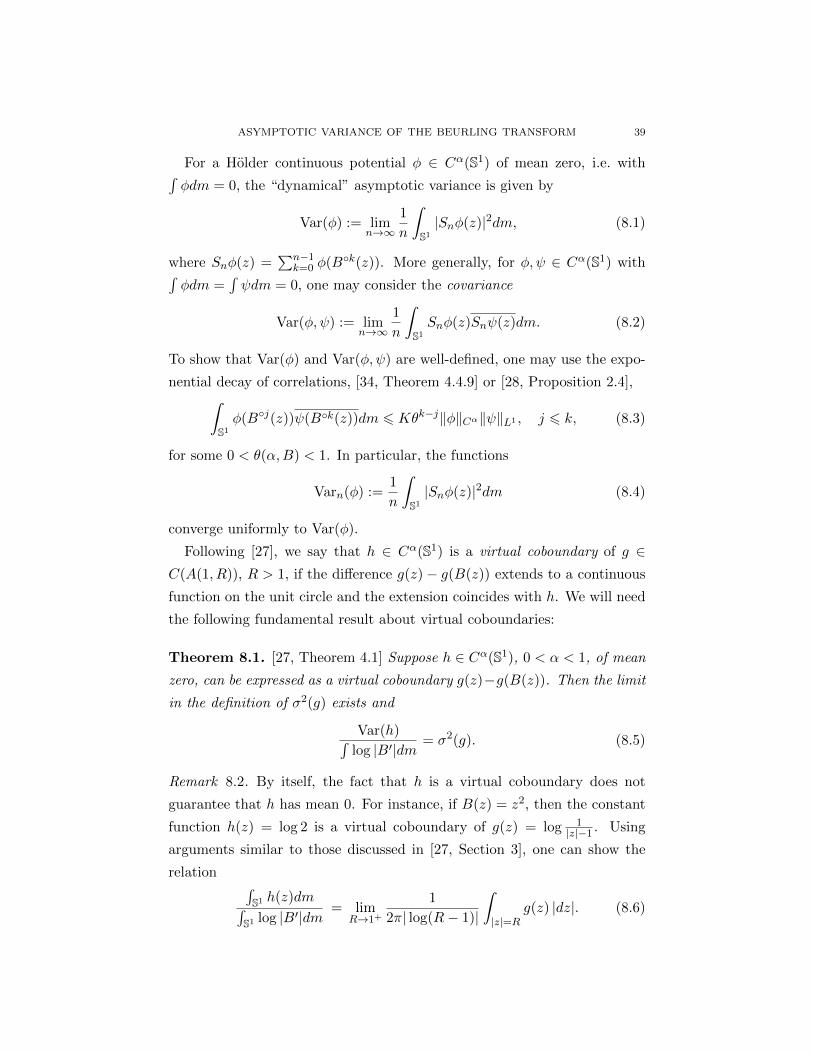
For a Holder continuous potential φ ∈ Cα(S1) of mean zero, i.e. with´φdm = 0, the “dynamical” asymptotic variance is given by
Var(φ) := limn→∞
1
n
ˆS1|Snφ(z)|2dm, (8.1)
where Snφ(z) =∑n−1
k=0 φ(Bk(z)). More generally, for φ, ψ ∈ Cα(S1) with´φdm =
´ψdm = 0, one may consider the covariance
Var(φ, ψ) := limn→∞
1
n
ˆS1Snφ(z)Snψ(z)dm. (8.2)
To show that Var(φ) and Var(φ, ψ) are well-defined, one may use the expo-
nential decay of correlations, [34, Theorem 4.4.9] or [28, Proposition 2.4],ˆS1φ(Bj(z))ψ(Bk(z))dm 6 Kθk−j‖φ‖Cα‖ψ‖L1 , j 6 k, (8.3)
for some 0 < θ(α,B) < 1. In particular, the functions
Varn(φ) :=1
n
ˆS1|Snφ(z)|2dm (8.4)
converge uniformly to Var(φ).
Following [27], we say that h ∈ Cα(S1) is a virtual coboundary of g ∈C(A(1, R)), R > 1, if the difference g(z)− g(B(z)) extends to a continuous
function on the unit circle and the extension coincides with h. We will need
the following fundamental result about virtual coboundaries:
Theorem 8.1. [27, Theorem 4.1] Suppose h ∈ Cα(S1), 0 < α < 1, of mean
zero, can be expressed as a virtual coboundary g(z)−g(B(z)). Then the limit
in the definition of σ2(g) exists and
Var(h)´log |B′|dm
= σ2(g). (8.5)
Remark 8.2. By itself, the fact that h is a virtual coboundary does not
guarantee that h has mean 0. For instance, if B(z) = z2, then the constant
function h(z) = log 2 is a virtual coboundary of g(z) = log 1|z|−1 . Using
arguments similar to those discussed in [27, Section 3], one can show the
relation ´S1 h(z)dm´
S1 log |B′|dm= lim
R→1+
1
2π| log(R− 1)|
ˆ|z|=R
g(z) |dz|. (8.6)
40 K. ASTALA, O. IVRII, A. PERALA, AND I. PRAUSE
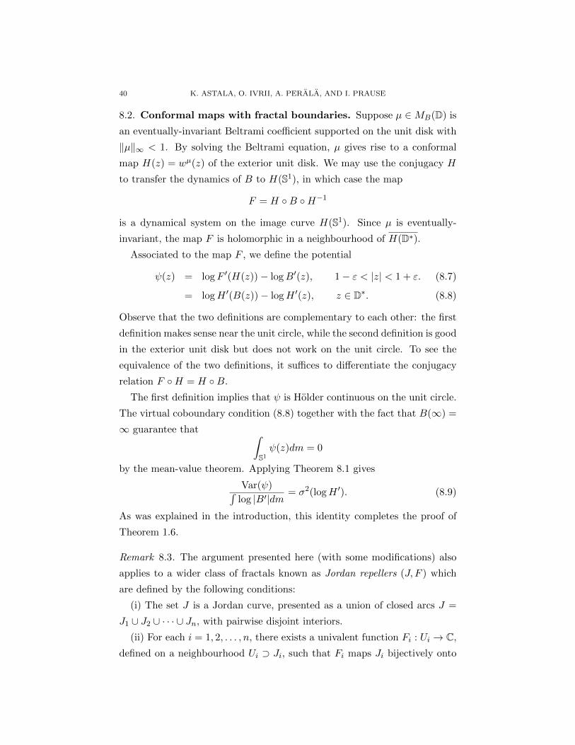
8.2. Conformal maps with fractal boundaries. Suppose µ ∈MB(D) is
an eventually-invariant Beltrami coefficient supported on the unit disk with
‖µ‖∞ < 1. By solving the Beltrami equation, µ gives rise to a conformal
map H(z) = wµ(z) of the exterior unit disk. We may use the conjugacy H
to transfer the dynamics of B to H(S1), in which case the map
F = H B H−1
is a dynamical system on the image curve H(S1). Since µ is eventually-
invariant, the map F is holomorphic in a neighbourhood of H(D∗).Associated to the map F , we define the potential
ψ(z) = logF ′(H(z))− logB′(z), 1− ε < |z| < 1 + ε. (8.7)
= logH ′(B(z))− logH ′(z), z ∈ D∗. (8.8)
Observe that the two definitions are complementary to each other: the first
definition makes sense near the unit circle, while the second definition is good
in the exterior unit disk but does not work on the unit circle. To see the
equivalence of the two definitions, it suffices to differentiate the conjugacy
relation F H = H B.
The first definition implies that ψ is Holder continuous on the unit circle.
The virtual coboundary condition (8.8) together with the fact that B(∞) =
∞ guarantee that ˆS1ψ(z)dm = 0
by the mean-value theorem. Applying Theorem 8.1 gives
Var(ψ)´log |B′|dm
= σ2(logH ′). (8.9)
As was explained in the introduction, this identity completes the proof of
Theorem 1.6.
Remark 8.3. The argument presented here (with some modifications) also
applies to a wider class of fractals known as Jordan repellers (J, F ) which
are defined by the following conditions:
(i) The set J is a Jordan curve, presented as a union of closed arcs J =
J1 ∪ J2 ∪ · · · ∪ Jn, with pairwise disjoint interiors.
(ii) For each i = 1, 2, . . . , n, there exists a univalent function Fi : Ui → C,defined on a neighbourhood Ui ⊃ Ji, such that Fi maps Ji bijectively onto
ASYMPTOTIC VARIANCE OF THE BEURLING TRANSFORM 41
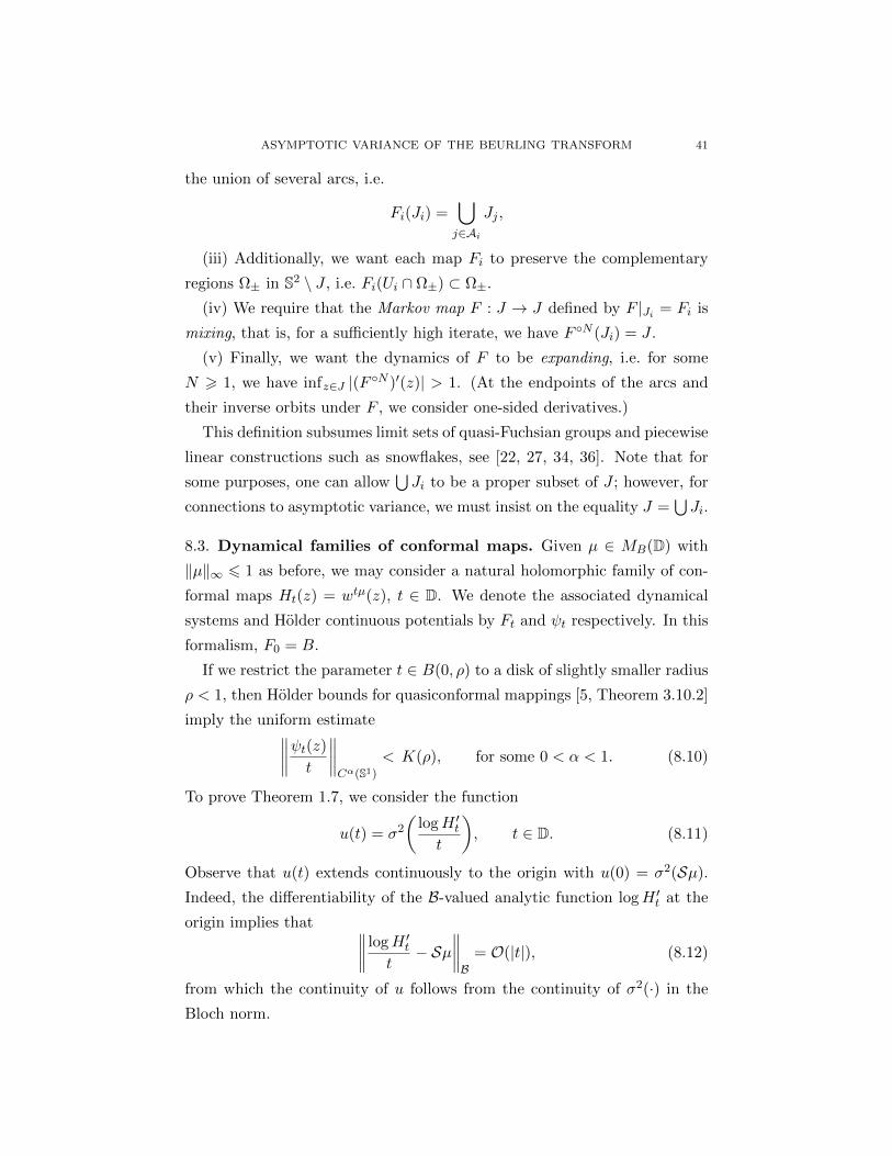
the union of several arcs, i.e.
Fi(Ji) =⋃j∈Ai
Jj ,
(iii) Additionally, we want each map Fi to preserve the complementary
regions Ω± in S2 \ J , i.e. Fi(Ui ∩ Ω±) ⊂ Ω±.
(iv) We require that the Markov map F : J → J defined by F |Ji = Fi is
mixing, that is, for a sufficiently high iterate, we have F N (Ji) = J .
(v) Finally, we want the dynamics of F to be expanding, i.e. for some
N > 1, we have infz∈J |(F N )′(z)| > 1. (At the endpoints of the arcs and
their inverse orbits under F , we consider one-sided derivatives.)
This definition subsumes limit sets of quasi-Fuchsian groups and piecewise
linear constructions such as snowflakes, see [22, 27, 34, 36]. Note that for
some purposes, one can allow⋃Ji to be a proper subset of J ; however, for
connections to asymptotic variance, we must insist on the equality J =⋃Ji.
8.3. Dynamical families of conformal maps. Given µ ∈ MB(D) with
‖µ‖∞ 6 1 as before, we may consider a natural holomorphic family of con-
formal maps Ht(z) = wtµ(z), t ∈ D. We denote the associated dynamical
systems and Holder continuous potentials by Ft and ψt respectively. In this
formalism, F0 = B.
If we restrict the parameter t ∈ B(0, ρ) to a disk of slightly smaller radius
ρ < 1, then Holder bounds for quasiconformal mappings [5, Theorem 3.10.2]
imply the uniform estimate∥∥∥∥ψt(z)t
∥∥∥∥Cα(S1)
< K(ρ), for some 0 < α < 1. (8.10)
To prove Theorem 1.7, we consider the function
u(t) = σ2
(logH ′tt
), t ∈ D. (8.11)
Observe that u(t) extends continuously to the origin with u(0) = σ2(Sµ).
Indeed, the differentiability of the B-valued analytic function logH ′t at the
origin implies that ∥∥∥∥ logH ′tt− Sµ
∥∥∥∥B
= O(|t|), (8.12)
from which the continuity of u follows from the continuity of σ2(·) in the
Bloch norm.
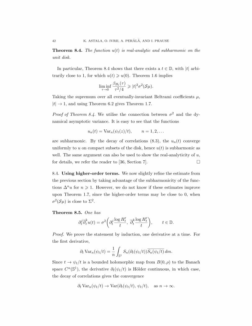
42 K. ASTALA, O. IVRII, A. PERALA, AND I. PRAUSE
Theorem 8.4. The function u(t) is real-analytic and subharmonic on the
unit disk.
In particular, Theorem 8.4 shows that there exists a t ∈ D, with |t| arbi-
trarily close to 1, for which u(t) > u(0). Theorem 1.6 implies
lim infτ→0
βHt(τ)
τ2/4> |t|2σ2(Sµ).
Taking the supremum over all eventually-invariant Beltrami coefficients µ,
|t| → 1, and using Theorem 6.2 gives Theorem 1.7.
Proof of Theorem 8.4. We utilise the connection between σ2 and the dy-
namical asymptotic variance. It is easy to see that the functions
un(t) = Varn(ψt(z)/t), n = 1, 2, . . .
are subharmonic. By the decay of correlations (8.3), the un(t) converge
uniformly to u on compact subsets of the disk, hence u(t) is subharmonic as
well. The same argument can also be used to show the real-analyticity of u,
for details, we refer the reader to [36, Section 7].
8.4. Using higher-order terms. We now slightly refine the estimate from
the previous section by taking advantage of the subharmonicity of the func-
tions ∆nu for n > 1. However, we do not know if these estimates improve
upon Theorem 1.7, since the higher-order terms may be close to 0, when
σ2(Sµ) is close to Σ2.
Theorem 8.5. One has
∂jt ∂kt u(t) = σ2
(∂jt
logH ′tt
, ∂kt
logH ′tt
), t ∈ D.
Proof. We prove the statement by induction, one derivative at a time. For
the first derivative,
∂t Varn(ψt/t) =1
n
ˆS1Sn(∂t(ψt/t))Sn(ψt/t) dm.
Since t → ψt/t is a bounded holomorphic map from B(0, ρ) to the Banach
space Cα(S1), the derivative ∂t(ψt/t) is Holder continuous, in which case,
the decay of correlations gives the convergence
∂t Varn(ψt/t)→ Var(∂t(ψt/t), ψt/t), as n→∞.
ASYMPTOTIC VARIANCE OF THE BEURLING TRANSFORM 43
To justify that ∂t Var(ψt/t) = Var(∂t(ψt/t), ψt/t), it suffices to use the well-
known fact that if a sequence of C1 functions Fn converges uniformly (on
compact sets) to F , and the derivatives F ′n converge uniformly to G, then
necessarily F ′ = G. One may compute further derivatives in the same
way.
Leveraging the subharmonicity of the functions ∆nu (which follows from
the previous theorem by taking j = k = n), the Poisson-Jensen formula for
subharmonic functions [37, Theorem 4.5.1] gives
lim supr→1
1
2π
ˆ|z|=r
u(z) |dz| > u(0) +∞∑n=1
c−1n ·∆nu(0), (8.13)
where cn = ∆n(|z|2n
). As noted earlier, u(0) = σ2(Sµ) while
∆u(0)
4= σ2
(SµSµ− 1
2(Sµ)2
)as the Neumann series expansion (3.2) shows. The Beltrami coefficient µ
from Lemma 5.5 (with the choice of degree d = 16) gives the value
lim infτ→0
B(τ)
τ2/4> σ2(Sµ) + σ2
(SµSµ− 1
2(Sµ)2
)> 0.893.
Using further terms, and playing around with the parameters (d, ρ0, n0),
we were able to (rigorously) obtain the lower bound 0.93 with the help of
Mathematica to automate the computations.
References
1. S. Abenda, P. Moussa, A. H. Osbaldestin, Multifractal dimensions and thermodynam-ical description of nearly-circular Julia sets, Nonlinearity 12 (1999), no. 1, 19–40.
2. S. Antonakoudis, Kra’s theta conjecture, preprint, 2014.3. K. Astala, Calderon’s problem for Lipschitz classes and the dimension of quasicircles,
Rev. Mat. Iberoamericana 4 (1988), no. 3-4, 469–486.4. K. Astala, Area distortion of quasiconformal mappings, Acta Math. 173 (1994), no. 1,
37–60.5. K. Astala, T. Iwaniec, G. J. Martin, Elliptic partial differential equations and quasi-
conformal mappings in the plane, Princeton University Press, 2009.6. K. Astala, T. Iwaniec, I. Prause, E. Saksman, Burkholder integrals, Morrey’s problem
and quasiconformal mappings, Journal of Amer. Mat. Soc. 25 (2011), no. 2, 507–531.7. K. Astala, T. Iwaniec, I. Prause, E. Saksman, Bilipschitz and quasiconformal rotation,
stretching and multifractal spectra, Publ. Math. Inst. Hautes Etudes Sci. (to appear).8. K. Astala, S. Rohde, O. Schramm, Self-similar Jordan curves, in preparation.9. J. Becker, C. Pommerenke, On the Hausdorff dimension of quasicircles, Ann. Acad.
Sci. Fenn. Ser. A I Math. 12 (1987), 329–333.10. L. Bers, H. Royden, Holomorphic families of injections, Acta Math. 157 (1986), 259–
286.11. I. Binder, Harmonic measure and rotation spectra of planar domains, preprint, 2008.
44 K. ASTALA, O. IVRII, A. PERALA, AND I. PRAUSE
12. H. Hedenmalm, Bloch functions and asymptotic variance, preprint, 2015.13. H. Hedenmalm, I. R. Kayumov, On the Makarov law of integrated logarithm, Proc.
Amer. Math. Soc. 135, (2007), 2235–2248.14. Y. Imayoshi, M. Taniguchi. An Introduction to Teichmuller Spaces, Springer-Verlag,
1992.15. O. Ivrii, The geometry of the Weil-Petersson metric in complex dynamics, preprint,
arXiv:1503.02590, 2015.16. D. Kalaj, D. Vujadinovic, Norm of the Bergman projection onto the Bloch space, J.
Operator Theory 73, no. 1, (2015), 113–126.17. I. R. Kayumov, The law of the iterated logarithm for locally univalent functions, Ann.
Acad. Sci. Fenn. Math. 27 (2002), no. 2, 357–364.18. R. Kuhnau, Moglichst konforme Spiegelung an einer Jordankurve, Jahresber. Deutsch.
Math.-Verein. 90 (1988), no. 2, 90–109.19. T. H. N. Le, M. Zinsmeister, On Minkowski dimension of Jordan curves, Ann. Acad.
Sci. Fenn. Math. 39 (2014), no. 2, 787–810.20. O. Lehto, Univalent functions and Teichmuller spaces, Springer, 1987.21. N. G. Makarov, Probability methods in the theory of conformal mappings, (Russian)
Algebra i Analiz 1 (1989), no. 1, 3–59; translation in Leningrad Math. J. 1 (1990), no.1, 1–56.
22. N. G. Makarov, Fine structure of harmonic measure, St. Petersburg Math. J. 10(1999), no. 2, 217–268.
23. R. Mane, P. Sad, D. Sullivan, On the dynamics of rational maps, Ann. Sci. EcoleNorm. Sup. (4) 16 (1983), no. 2, 193–217.
24. C. T. McMullen, Amenability, Poincare series and quasiconformal maps, Invent.math. 97 (1989), 95–127.
25. C. T. McMullen, Cusps are dense, Ann. Math. 133 (1991), 217–247.26. C. T. McMullen, The moduli space of Riemann surfaces is Kahler hyperbolic, Ann.
Math. 151 (2000), 327–357.27. C. T. McMullen, Thermodynamics, dimension and the Weil-Petersson metric, Invent.
Math. 173 (2008), no. 2, 365–425.28. W. Parry, M. Pollicott, Zeta Functions and the Periodic Orbit Structure of Hyperbolic
Dynamics, Asterisque, vol. 187–188, 1990.29. A. Perala, On the optimal constant for the Bergman projection onto the Bloch space,
Ann. Acad. Sci. Fenn. Math. 37 (2012), no. 1, 245–249.30. J. A. Pfaltzgraff, Univalence of the integral of f ′(z)λ, Bull. London Math. Soc. 7
(1975), 254–256.31. C. Pommerenke, Boundary behaviour of conformal maps, Grundlehren der Mathema-
tischen Wissenschaften 299, Springer-Verlag, 1992.32. I. Prause, S. Smirnov, Quasisymmetric distortion spectrum, Bull. Lond. Math. Soc.
43 (2011), 267–277.33. I. Prause, X. Tolsa, I. Uriarte-Tuero, Hausdorff measure of quasicircles, Adv. Math.
229 (2012), no. 2, 1313–1328.34. F. Przytycki, M. Urbanski, Conformal Fractals – Ergodic Theory Methods, 2009.35. F. Przytycki, M. Urbanski, A. Zdunik, Harmonic, Gibbs and Hausdorff measures on
repellers for holomorphic maps I, Ann. Math. 130 (1989), 1–40.36. F. Przytycki, M. Urbanski, A. Zdunik, Harmonic, Gibbs and Hausdorff measures on
repellers for holomorphic maps II, Studia Math. 97 (1991), 189–225.37. T. Ransford, Potential Theory in the Complex Plane, London Mathematical Society
Student Texts, Cambridge University Press, 1995.38. E. Reich, Extremal quasiconformal mappings of the disk, in Handbook of Complex
Analysis: Geometric Function Theory, vol. 1, North-Holland, 75–136, 2002.39. D. Ruelle, Repellers for real analytic maps, Erg. Th. & Dyn. Sys. 2 (1982), no. 1,
99–107.
ASYMPTOTIC VARIANCE OF THE BEURLING TRANSFORM 45
40. Z. Slodkowski, Holomorphic motions and polynomial hulls, Proc. Amer. Math. Soc.111 (1991), 347–355.
41. S. Smirnov, Dimension of quasicircles, Acta Math. 205 (2010), no. 1, 189–197.
Le Studiumr, Loire Valley Institute for Advanced Studies, Orleans &Tours, France; Mapmo, rue de Chartres, 45100 Orleans, France; Departmentof Mathematics and Statistics, University of Helsinki, P.O. Box 68, FIN-00014,Helsinki, Finland
E-mail address: [email protected]
Department of Mathematics and Statistics, University of Helsinki, P.O.Box 68, FIN-00014, Helsinki, Finland
E-mail address: [email protected]
Department of Mathematics and Statistics, University of Helsinki, P.O.Box 68, FIN-00014, Helsinki, Finland
E-mail address: [email protected]
Department of Mathematics and Statistics, University of Helsinki, P.O.Box 68, FIN-00014, Helsinki, Finland
E-mail address: [email protected]