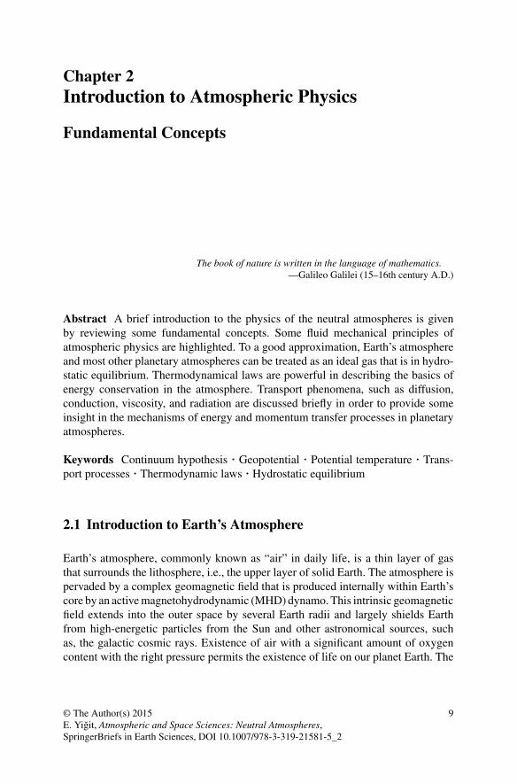
Chapter 2Introduction to Atmospheric Physics

Fundamental Concepts

The book of nature is written in the language of mathematics.—Galileo Galilei (15–16th century A.D.)

Abstract A brief introduction to the physics of the neutral atmospheres is givenby reviewing some fundamental concepts. Some fluid mechanical principles ofatmospheric physics are highlighted. To a good approximation, Earth’s atmosphereand most other planetary atmospheres can be treated as an ideal gas that is in hydro-static equilibrium. Thermodynamical laws are powerful in describing the basics ofenergy conservation in the atmosphere. Transport phenomena, such as diffusion,conduction, viscosity, and radiation are discussed briefly in order to provide someinsight in the mechanisms of energy and momentum transfer processes in planetaryatmospheres.

Keywords Continuum hypothesis · Geopotential · Potential temperature · Trans-port processes · Thermodynamic laws · Hydrostatic equilibrium

2.1 Introduction to Earth’s Atmosphere

Earth’s atmosphere, commonly known as “air” in daily life, is a thin layer of gasthat surrounds the lithosphere, i.e., the upper layer of solid Earth. The atmosphere ispervaded by a complex geomagnetic field that is produced internally within Earth’score by an activemagnetohydrodynamic (MHD) dynamo. This intrinsic geomagneticfield extends into the outer space by several Earth radii and largely shields Earthfrom high-energetic particles from the Sun and other astronomical sources, suchas, the galactic cosmic rays. Existence of air with a significant amount of oxygencontent with the right pressure permits the existence of life on our planet Earth. The

© The Author(s) 2015E. Yigit, Atmospheric and Space Sciences: Neutral Atmospheres,SpringerBriefs in Earth Sciences, DOI 10.1007/978-3-319-21581-5_2

9

10 2 Introduction to Atmospheric Physics

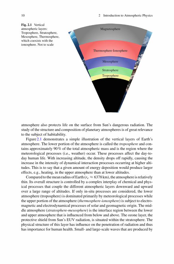
Fig. 2.1 Verticalatmospheric layers:Troposphere, Stratosphere,Mesosphere, Thermosphere,which coexists with theionosphere. Not to scale

Magnetosphere

Thermosphere-Ionosphere

Mesosphere

Stratosphere

Troposphere

atmosphere also protects life on the surface from Sun’s dangerous radiation. Thestudy of the structure and composition of planetary atmospheres is of great relevanceto the subject of habitability.

Figure2.1 demonstrates a simple illustration of the vertical layers of Earth’satmosphere. The lower portion of the atmosphere is called the troposphere and con-tains approximately 90% of the total atmospheric mass and is the region where themeteorological processes (i.e., weather) occur. These processes affect the day-to-day human life. With increasing altitude, the density drops off rapidly, causing theincrease in the intensity of dynamical interaction processes occurring at higher alti-tudes. This is to say that a given amount of energy deposition would produce largereffects, e.g., heating, in the upper atmosphere than at lower altitudes.

Compared to themean radius ofEarth (re ≈ 6378km), the atmosphere is relativelythin. Its overall structure is controlled by a complex interplay of chemical and phys-ical processes that couple the different atmospheric layers downward and upwardover a large range of altitudes. If only in-situ processes are considered, the loweratmosphere (troposphere) is dominated primarily by meteorological processes whilethe upper portion of the atmosphere (thermosphere-ionosphere) is subject to electro-magnetic and electrodynamical processes of solar and geomagnetic origin. The mid-dle atmosphere (stratosphere-mesosphere) is the interface region between the lowerand upper atmosphere that is influenced from below and above. The ozone layer, theprotective shield from Sun’s EUV radiation, is situated within the stratosphere. Thephysical structure of this layer has influence on the penetration of radiation and thushas importance for human health. Small- and large-scale waves that are produced by

2.1 Introduction to Earth’s Atmosphere 11

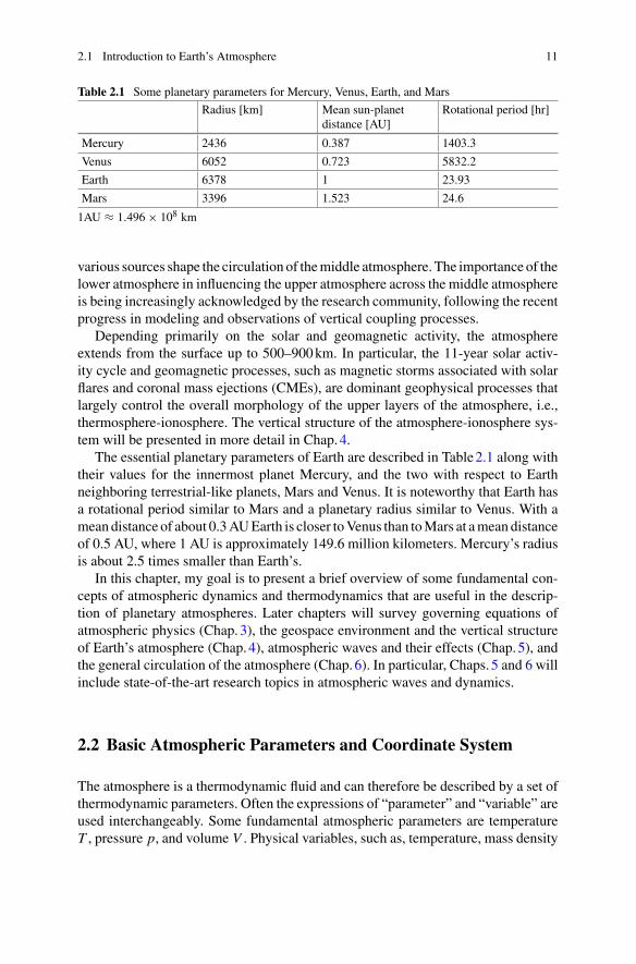
Table 2.1 Some planetary parameters for Mercury, Venus, Earth, and Mars

Radius [km] Mean sun-planetdistance [AU]

Rotational period [hr]

Mercury 2436 0.387 1403.3

Venus 6052 0.723 5832.2

Earth 6378 1 23.93

Mars 3396 1.523 24.6

1AU ≈ 1.496 × 108 km

various sources shape the circulation of themiddle atmosphere. The importance of thelower atmosphere in influencing the upper atmosphere across the middle atmosphereis being increasingly acknowledged by the research community, following the recentprogress in modeling and observations of vertical coupling processes.

Depending primarily on the solar and geomagnetic activity, the atmosphereextends from the surface up to 500–900km. In particular, the 11-year solar activ-ity cycle and geomagnetic processes, such as magnetic storms associated with solarflares and coronal mass ejections (CMEs), are dominant geophysical processes thatlargely control the overall morphology of the upper layers of the atmosphere, i.e.,thermosphere-ionosphere. The vertical structure of the atmosphere-ionosphere sys-tem will be presented in more detail in Chap.4.

The essential planetary parameters of Earth are described in Table2.1 along withtheir values for the innermost planet Mercury, and the two with respect to Earthneighboring terrestrial-like planets, Mars and Venus. It is noteworthy that Earth hasa rotational period similar to Mars and a planetary radius similar to Venus. With amean distance of about 0.3AUEarth is closer toVenus than toMars at amean distanceof 0.5 AU, where 1 AU is approximately 149.6 million kilometers. Mercury’s radiusis about 2.5 times smaller than Earth’s.

In this chapter, my goal is to present a brief overview of some fundamental con-cepts of atmospheric dynamics and thermodynamics that are useful in the descrip-tion of planetary atmospheres. Later chapters will survey governing equations ofatmospheric physics (Chap. 3), the geospace environment and the vertical structureof Earth’s atmosphere (Chap.4), atmospheric waves and their effects (Chap. 5), andthe general circulation of the atmosphere (Chap.6). In particular, Chaps. 5 and 6 willinclude state-of-the-art research topics in atmospheric waves and dynamics.

2.2 Basic Atmospheric Parameters and Coordinate System

The atmosphere is a thermodynamic fluid and can therefore be described by a set ofthermodynamic parameters. Often the expressions of “parameter” and “variable” areused interchangeably. Some fundamental atmospheric parameters are temperatureT , pressure p, and volume V . Physical variables, such as, temperature, mass density

12 2 Introduction to Atmospheric Physics

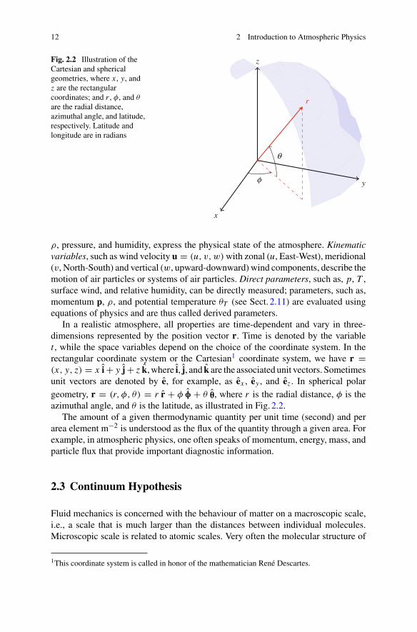
Fig. 2.2 Illustration of theCartesian and sphericalgeometries, where x , y, andz are the rectangularcoordinates; and r , φ, and θ

are the radial distance,azimuthal angle, and latitude,respectively. Latitude andlongitude are in radians

x

y

z

r

φ

θ

ρ, pressure, and humidity, express the physical state of the atmosphere. Kinematicvariables, such as wind velocity u = (u, v, w)with zonal (u, East-West), meridional(v, North-South) and vertical (w, upward-downward) wind components, describe themotion of air particles or systems of air particles. Direct parameters, such as, p, T ,surface wind, and relative humidity, can be directly measured; parameters, such as,momentum p, ρ, and potential temperature θT (see Sect. 2.11) are evaluated usingequations of physics and are thus called derived parameters.

In a realistic atmosphere, all properties are time-dependent and vary in three-dimensions represented by the position vector r. Time is denoted by the variablet , while the space variables depend on the choice of the coordinate system. In therectangular coordinate system or the Cartesian1 coordinate system, we have r =(x, y, z) = x i + y j + z k,where i, j, and k are the associated unit vectors. Sometimesunit vectors are denoted by e, for example, as ex , ey , and ez . In spherical polargeometry, r = (r, φ, θ) = r r + φ φ + θ θ, where r is the radial distance, φ is theazimuthal angle, and θ is the latitude, as illustrated in Fig. 2.2.

The amount of a given thermodynamic quantity per unit time (second) and perarea element m−2 is understood as the flux of the quantity through a given area. Forexample, in atmospheric physics, one often speaks of momentum, energy, mass, andparticle flux that provide important diagnostic information.

2.3 Continuum Hypothesis

Fluid mechanics is concerned with the behaviour of matter on a macroscopic scale,i.e., a scale that is much larger than the distances between individual molecules.Microscopic scale is related to atomic scales. Very often the molecular structure of

1This coordinate system is called in honor of the mathematician René Descartes.

2.3 Continuum Hypothesis 13

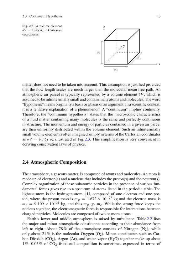
Fig. 2.3 A volume elementδV = δx δy δz in Cartesiancoordinates

x

y

z

δ x

δ z

δ y

matter does not need to be taken into account. This assumption is justified providedthat the flow length scales are much larger than the molecular mean free path. Anatmospheric air parcel is typically represented by a volume element δV , which isassumed to be infinitesimally small and containmany atoms andmolecules. Theword“hypothesis”means originally a basis or a basis of an argument. In a scientific context,it is a tentative explanation of a phenomenon. A “continuum” implies continuity.Therefore, the “continuum hypothesis” states that the macroscopic characteristicsof a fluid matter containing many molecules is the same and perfectly continuousin structure. The momentum and energy of particles contained in a given air parcelare then uniformly distributed within the volume element. Such an infinitesimallysmall volume element is often imagined simply in terms of the Cartesian coordinatesas δV = δx δy δz illustrated in Fig. 2.3. This simplification is very convenient inderiving conservation laws of physics.

2.4 Atmospheric Composition

The atmosphere, a gaseous matter, is composed of atoms and molecules. An atom ismade up of electron(s) and a nucleus that includes the proton(s) and the neutron(s).Complex organization of these subatomic particles in the presence of various fun-damental forces gives rise to a spectrum of atoms listed in the periodic table. Thelightest atom is the hydrogen atom, 1

1H, composed of one electron and one pro-ton, where the proton mass is m p = 1.672 × 10−27 kg and the electron mass isme = 9.109 × 10−31 kg, and thus m p � me. While the strong force keeps thenucleus together, the electromagnetic force is responsible for interactions betweencharged particles. Molecules are composed of two or more atoms.

Earth’s lower and middle atmosphere is mixed by turbulence. Table2.2 liststhe major and minor atmospheric constituents according to their abundance fromleft to right. About 78% of the atmosphere consists of Nitrogen (N2), whileonly about 21% is the molecular Oxygen (O2). Minor constituents such as Car-bon Dioxide (CO2), Argon (Ar), and water vapor (H2O) together make up about1%. 0.03% of CO2 fractional composition is sometimes expressed in terms of

14 2 Introduction to Atmospheric Physics

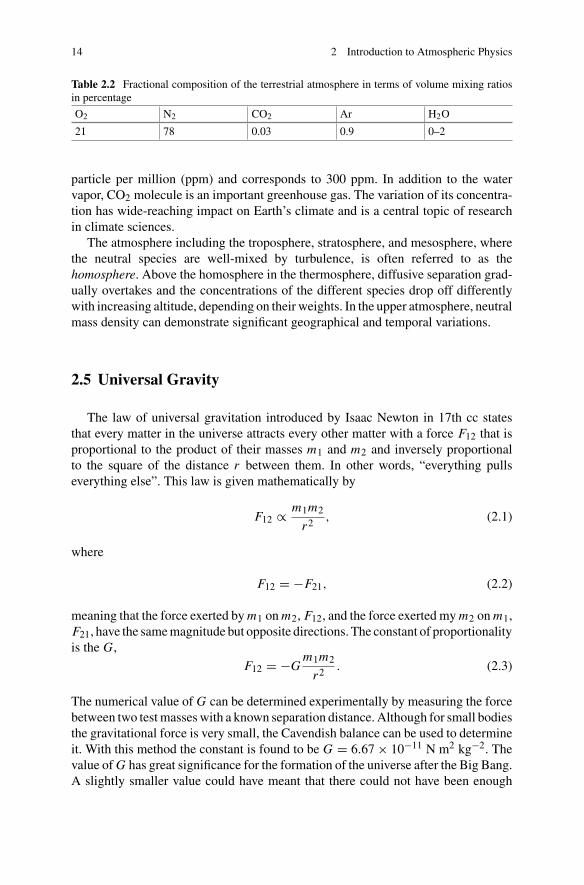
Table 2.2 Fractional composition of the terrestrial atmosphere in terms of volume mixing ratiosin percentage

O2 N2 CO2 Ar H2O

21 78 0.03 0.9 0–2

particle per million (ppm) and corresponds to 300 ppm. In addition to the watervapor, CO2 molecule is an important greenhouse gas. The variation of its concentra-tion has wide-reaching impact on Earth’s climate and is a central topic of researchin climate sciences.

The atmosphere including the troposphere, stratosphere, and mesosphere, wherethe neutral species are well-mixed by turbulence, is often referred to as thehomosphere. Above the homosphere in the thermosphere, diffusive separation grad-ually overtakes and the concentrations of the different species drop off differentlywith increasing altitude, depending on their weights. In the upper atmosphere, neutralmass density can demonstrate significant geographical and temporal variations.

2.5 Universal Gravity

The law of universal gravitation introduced by Isaac Newton in 17th cc statesthat every matter in the universe attracts every other matter with a force F12 that isproportional to the product of their masses m1 and m2 and inversely proportionalto the square of the distance r between them. In other words, “everything pullseverything else”. This law is given mathematically by

F12 ∝ m1m2

r2, (2.1)

where

F12 = −F21, (2.2)

meaning that the force exerted by m1 on m2, F12, and the force exerted my m2 on m1,F21, have the samemagnitude but opposite directions. The constant of proportionalityis the G,

F12 = −Gm1m2

r2. (2.3)

The numerical value of G can be determined experimentally by measuring the forcebetween two testmasseswith a known separation distance. Although for small bodiesthe gravitational force is very small, the Cavendish balance can be used to determineit. With this method the constant is found to be G = 6.67 × 10−11 N m2 kg−2. Thevalue of G has great significance for the formation of the universe after the Big Bang.A slightly smaller value could have meant that there could not have been enough

2.5 Universal Gravity 15

gravitational force between matter to clump together to form more complex matter.A stronger G could have implied that the expansion of the universe could have nottaken place.

In terms of fundamental particles, you can consider the gravitational attractionbetween a proton and an electron, which amounts to∼10−47 N at an atomic distanceof 1 Å. In planetary atmospheres, the most obvious effect of gravity is that everthingis accelerated toward the center of the planet and it is a body force in the equationof motion. The associated acceleration of the mass m in a planet of mass M due tothe force FMm exerted by the planet on m is

g = FMm

m= G

M

r2, (2.4)

where the distance r = rp + z is the sum of planetary radius and the altitude from thesurface. For Earth, with Me = 5.97 × 1024 kg the mean gravitational accelerationon the surface is g0 ≈ 9.80m s−2. For Mars, with Mm = 0.1 Me and rm = re/2the mean surface gravitation acceleration is 3.92m s−2, which is 2.5 smaller thanon Earth. The altitude variation of the gravitational acceleration is approximatelygiven by

g(z) = g01 + z

rE

, (2.5)

For z � rE we have g ≈ g0.

2.6 Equation of State: Ideal Gas Law

A relation between the fundamental thermodynamic variables, such as, pressure p,temperatureT , volumeV , andnumber of particles (molecules) N in a thermodynamicsystem is given by an equation of state f as

f (p, T, V, N ) = 0. (2.6)

This property states that only a certain number of the properties of a substance can begiven arbitrary values in a thermodynamic system. The specific form of an equationof state depends on the substance.

An ideal gas is defined in an atomistic view as a collection of gas of any speciesin which no forces operate between the individual gas particles. It has been exper-imentally found that there is a distinct relationship between the pressure and thetemperature of an ideal gas. Namely, pressure times molal specific volume ν (i.e.,volume per mole V/n) divided by temperature is equal to a constant R

pν

T= R, (2.7)

16 2 Introduction to Atmospheric Physics

where the universal gas constant R is

R = 8.317 J mole−1K−1. (2.8)

Because there are a large number of atoms in a given volume, chemists have intro-duced the concept of “mole” in order to count more easily. One mole containsNA = 6.02 × 1023 particles, where NA is known as Avogadro’s number2 and isdefined by the number of carbon-12 atoms contained exactly in 12g of carbon-12(126 C). So the amount of matter in a volume element can be measured in terms ofmoles as well. For example, a mole of oxygen 16

8 O is 16 g. The number of atoms ina mole times the Boltzmann constant yields the universal gas constant R

R = NAkb, (2.9)

where the Boltzmann constant kb = 1.381 × 10−23 J K−1. In turn, at a fixed tem-perature and volume, the total number of atoms can be determined.

The ideal gas law in terms of the volume and the number of moles is then

pV = n RT . (2.10)

Equation (2.10) can be expressed in terms of the density ρ, which is of interest inplanetary atmospheres. With V = m/ρ combined with an expression for the totalmass m in terms of the mean molecular mass mm as n = m/mm , we can expressvolume

V = nmm

ρ, (2.11)

and substitute in (2.10), which yields

p = ρR

mmT . (2.12)

The mean molecular mass varies with altitude in planetary atmospheres. On Earth,mm ≈ 28.8 g mol−1 in the lower and middle atmosphere and decreases in thethermosphere. For practical calculations a typical value of mm can be assumed todefine

R∗ = R

mm≈ 288.7 J kg−1 K−1, (2.13)

yielding a simplified equation of state for an ideal gas

p = ρR∗T . (2.14)

2Named after the Italian physicist Amedeo Avogadro.

2.6 Equation of State: Ideal Gas Law 17

The ideal gas law is a limiting case for the behaviour of a real gas, which isdescribed by the Van der Vaals law. For planetary atmospheres, the ideal gas law isa very good approximation.

At constant temperature, pressure is inversely proportional to volume

p ∝ V −1, (2.15)

called the Boyle-Mariotte law. At constant volume, pressure is proportional to tem-perature

p ∝ T, (2.16)

referred to as the Guy-Lussac law.

2.7 Thermodynamic Laws

Thermodynamics is the branch of physics that studies the relationship among the var-ious properties of matter, without the knowledge of internal structure of the matter.The laws of thermodynamics contain qualitatively all the principles of thermodynam-ics. The first law of thermodynamics states that the conservation of energy given by

ΔU = ΔQ + ΔW, (2.17)

where ΔU , ΔQ, and ΔW are the changes in internal energy, heat flow, and in workdone. This law states that the total change in the internal energy of a system is givenby the sums of changes in heat flow and the work done. The differential form of(2.17) is then

dU = dQ + dW, (2.18)

where dW = −pdV is the work done on the system.The second law of thermodynamics originally hypothesized by Carnot implies

that heat on its own cannot flow from a cold to a warm object. This is the conceptthat is familiar to us from the day-to-day life. In a hot summer day, if you leave thebalcony door open, then your room that had been cooled by an air conditioner willwarm up by heat flow from outside into the room. Specifically, the entropy (disorder)in an isolated system either increases or remains constant.

A thermodynamical system can be taken from one state to another state by variousthermal and/or dynamical processes. This change can take place in different ways.For example, in adiabatic processes, the temperature of a system is independent ofits environment and the kinetic and potential energy of the system do not change.

18 2 Introduction to Atmospheric Physics

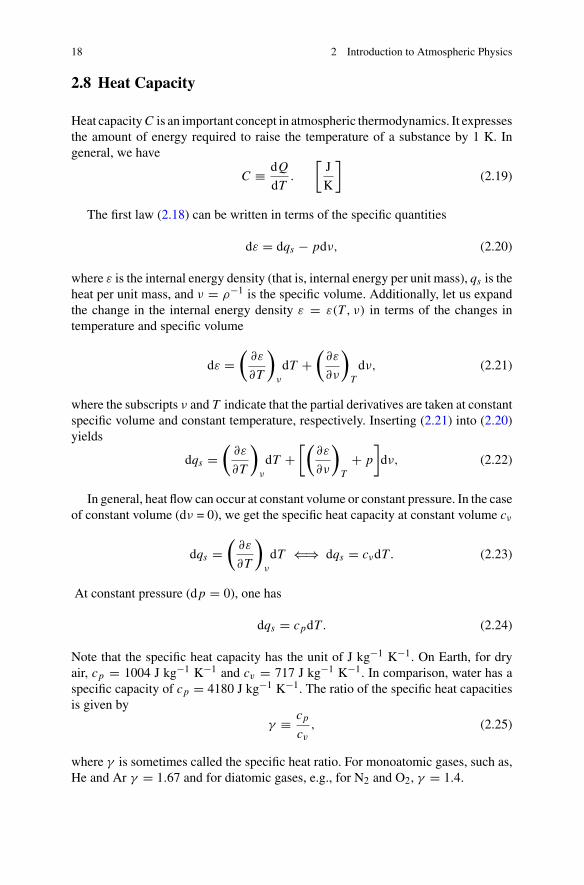
2.8 Heat Capacity

Heat capacityC is an important concept in atmospheric thermodynamics. It expressesthe amount of energy required to raise the temperature of a substance by 1 K. Ingeneral, we have

C ≡ dQ

dT.

[J

K

](2.19)

The first law (2.18) can be written in terms of the specific quantities

dε = dqs − pdν, (2.20)

where ε is the internal energy density (that is, internal energy per unit mass), qs is theheat per unit mass, and ν = ρ−1 is the specific volume. Additionally, let us expandthe change in the internal energy density ε = ε(T, ν) in terms of the changes intemperature and specific volume

dε =(

∂ε

∂T

)ν

dT +(

∂ε

∂ν

)Tdν, (2.21)

where the subscripts ν and T indicate that the partial derivatives are taken at constantspecific volume and constant temperature, respectively. Inserting (2.21) into (2.20)yields

dqs =(

∂ε

∂T

)ν

dT +[(

∂ε

∂ν

)T

+ p

]dν, (2.22)

In general, heat flow can occur at constant volume or constant pressure. In the caseof constant volume (dν = 0), we get the specific heat capacity at constant volume cν

dqs =(

∂ε

∂T

)ν

dT ⇐⇒ dqs = cνdT . (2.23)

At constant pressure (dp = 0), one has

dqs = cpdT . (2.24)

Note that the specific heat capacity has the unit of J kg−1 K−1. On Earth, for dryair, cp = 1004 J kg−1 K−1 and cv = 717 J kg−1 K−1. In comparison, water has aspecific capacity of cp = 4180 J kg−1 K−1. The ratio of the specific heat capacitiesis given by

γ ≡ cp

cv

, (2.25)

where γ is sometimes called the specific heat ratio. For monoatomic gases, such as,He and Ar γ = 1.67 and for diatomic gases, e.g., for N2 and O2, γ = 1.4.

2.9 Geopotential 19

2.9 Geopotential

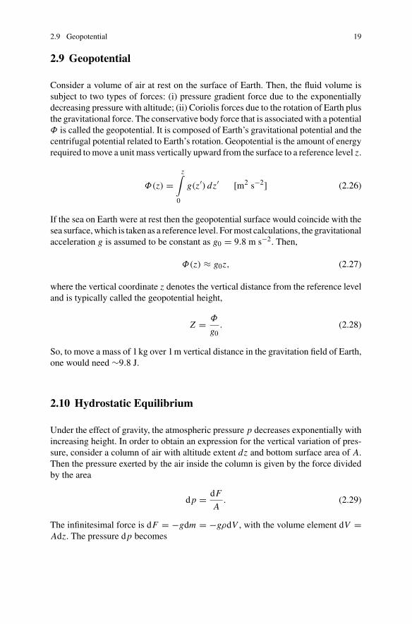
Consider a volume of air at rest on the surface of Earth. Then, the fluid volume issubject to two types of forces: (i) pressure gradient force due to the exponentiallydecreasing pressure with altitude; (ii) Coriolis forces due to the rotation of Earth plusthe gravitational force. The conservative body force that is associated with a potentialΦ is called the geopotential. It is composed of Earth’s gravitational potential and thecentrifugal potential related to Earth’s rotation. Geopotential is the amount of energyrequired tomove a unit mass vertically upward from the surface to a reference level z.

Φ(z) =z∫

0

g(z′) dz′ [m2 s−2] (2.26)

If the sea on Earth were at rest then the geopotential surface would coincide with thesea surface,which is taken as a reference level. Formost calculations, the gravitationalacceleration g is assumed to be constant as g0 = 9.8 m s−2. Then,

Φ(z) ≈ g0z, (2.27)

where the vertical coordinate z denotes the vertical distance from the reference leveland is typically called the geopotential height,

Z = Φ

g0. (2.28)

So, to move a mass of 1kg over 1m vertical distance in the gravitation field of Earth,one would need ∼9.8 J.

2.10 Hydrostatic Equilibrium

Under the effect of gravity, the atmospheric pressure p decreases exponentially withincreasing height. In order to obtain an expression for the vertical variation of pres-sure, consider a column of air with altitude extent dz and bottom surface area of A.Then the pressure exerted by the air inside the column is given by the force dividedby the area

dp = dF

A. (2.29)

The infinitesimal force is dF = −gdm = −gρdV , with the volume element dV =Adz. The pressure dp becomes

20 2 Introduction to Atmospheric Physics

dp = dF

A= −g ρ A dz

A. (2.30)

The hydrostatic equilibrium (or balance) is then given by

dp

dz= −gρ. (2.31)

Equation (2.31) expresses that the downward gravitational acceleration is balancedby the upward directed acceleration associated with the negative upward pressuregradient. Without Earth’s gravity, air would be accelerated into space. Hydrostaticacceleration implies that the vertical acceleration of air is negligible, though verticalair speed can be non-zero. In processes that may involve nonhydrostatic effects(e.g.,Yigit and Ridley 2011) the hydrostatic condition (2.31) does not apply.

From the hydrostatic relation, the vertical variation of pressure can be derived.Applying separation of variables in (2.31), representing the density with the ideal gaslaw (2.12) and then writing with the left-hand side and right-hand side with integralswith limits from some reference levels p0 to p and z0 to z, respectively, give

p∫p0

dp

p= −

z∫z0

m(z) g(z)

R T (z)dz, (2.32)

and finally integrating the left-hand side with respect to pressure yields

p(z) = p0 exp

(−

z∫z0

mg

RTdz

), (2.33)

in terms of the scale height H

H ≡ RT

mg, (2.34)

we get

p(z) = p0 exp

(−

z∫z0

1

H(z)dz

). (2.35)

Over small vertical distances, the scale height may vary slowly in the loweratmosphere and can be assumed to be constant for practical purposes. Equation(2.35) can be approximated

p(z) = p0 exp

(− z − z0

H

), (2.36)

2.10 Hydrostatic Equilibrium 21

which shows that the pressure falls off exponentially with height. In the upperatmosphere, because of diffusive separation, one speaks of the individual scaleheights of the different species. For a neutral species i with molecular mass mi ,we then have

Hi (z) = R T (z)

mi g(z)(2.37)

Overall, the scale height can vary significantly with height because of the largevariations of temperature and the mean molecular mass with height. The concept ofscale height also applies to ionized species.

2.11 Potential Temperature

The potential temperature is the temperature a parcel of air at pressure p and temper-ature T would obtain if it were expanded or compressed adiabatically to a standardpressure ps = 1000 hPa.

θT = T

(ps

p

)R/cp

, (2.38)

where cp is the specific heat at constant pressure and T is temperature. Equation(2.38) is known as Poisson equation as well. For dry adiabatic conditions, the poten-tial temperature is conserved. Sometimes, instead of temperature and pressure, poten-tial temperature and pressure are used as state variables. Also, the stability of theatmosphere is measured in terms of the potential temperature gradient.

2.12 Atmospheric Stability

The variation of neutral temperature with altitude in a planetary atmosphere is animportant criterion that shapes the stability of the atmosphere.

2.12.1 Lapse Rate

Temperature lapse rate Γ describes the rate of temperature decrease with increasingaltitude:

Γ = −∂T

∂z(2.39)

22 2 Introduction to Atmospheric Physics

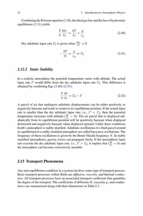
Combining thePoisson equation (2.38), the ideal gas lawand the lawof hydrostaticequilibrium (2.31) yields

T

θ

∂θT

∂z= ∂T

∂z+ g

cp(2.40)

Dry adiabatic lapse rate Γd is given when ∂θT∂z = 0

− ∂T

∂z= g

cp≡ Γd (2.41)

2.12.2 Static Stability

In a realistic atmosphere the potential temperature varies with altitude. The actuallapse rate Γ would differ from the dry adiabatic lapse rate Γd . This difference isobtained by combining Eqs. (2.40)–(2.41):

T

θ

∂θ

∂z= Γd − Γ (2.42)

A parcel of air that undergoes adiabatic displacements can be either positively ornegatively buoyant and tends to return to its equilibrium position. If the actual lapserate is smaller than the dry adiabatic lapse rate, i.e., Γ < Γd , then the potentialtemperature increases with altitude ( ∂θ

∂z > 0). The air parcel that is displaced adi-abatically from its equilibrium position will be positively buoyant when displaceddownward and negatively buoyant when displaced upward. Under these conditionsEarth’s atmosphere is stably stratified. Adiabatic oscillations of a fluid parcel aroundits equilibrium in a stably stratified atmosphere are called buoyancy oscillations. Thefrequency of these oscillations is given by the Brunt-Väisälä frequency N . In stablystratified atmospheres, gravity waves can propagate freely. If the atmospheric lapserate exceeds the dry adiabatic lapse rate, i.e., Γ > Γd , it implies that ( ∂θ

∂z < 0) andthe atmosphere can become convectively unstable.

2.13 Transport Phenomena

Any non-equilibrium condition in a system involves some type of transport process.Basic transport processes within fluids are diffusion, viscosity, and thermal conduc-tion. All transport processes have an associated transport coefficient that quantifiesthe degree of the transport. The coefficients of diffusion D, viscosity μ, and conduc-tion κ are summarized along with their dimensions in Table2.3.

2.13 Transport Phenomena 23

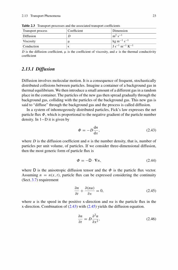
Table 2.3 Transport processes and the associated transport coefficients

Transport process Coefficient Dimension

Diffusion D m2 s−1

Viscosity μ kg m−1 s−1

Conduction κ J s−1 m−1 K−1

D is the diffusion coefficient, μ is the coefficient of viscosity, and κ is the thermal conductivitycoefficient

2.13.1 Diffusion

Diffusion involves molecular motion. It is a consequence of frequent, stochasticallydistributed collisions between particles. Imagine a container of a background gas inthermal equilibrium.We then introduce a small amount of a different gas in a randomplace in the container. The particles of the new gas then spread gradually through thebackground gas, colliding with the particles of the background gas. This new gas issaid to “diffuse” through the background gas and the process is called diffusion.

In a system of inhomogeously distributed particles, Fick’s law expresses the netparticle flux Φ, which is proportional to the negative gradient of the particle numberdensity. In 1−D it is given by

Φ = −Ddn

dx, (2.43)

where D is the diffusion coefficient and n is the number density, that is, number ofparticles per unit volume, of particles. If we consider three-dimensional diffusion,then the most generic form of particle flux is

Φ = −D · ∇n, (2.44)

where D is the anisotropic diffusion tensor and the Φ is the particle flux vector.Assuming n = n(x, t), particle flux can be expressed considering the continuity(Sect. 3.7) requirement

∂n

∂t+ ∂(nu)

∂x= 0, (2.45)

where u is the speed in the positive x-direction and nu is the particle flux in thex-direction. Combination of (2.43) with (2.45) yields the diffusion equation.

∂n

∂t= D

∂2n

∂x2, (2.46)

24 2 Introduction to Atmospheric Physics

assuming isotropic homogeneous diffusion. In three dimensions one gets

∂n

∂t= D ∇2n, (2.47)

where ∇2 = ∂2

∂x2+ ∂2

∂y2+ ∂2

∂z2is the Laplace operator in Cartesian coordinates.

In processes that involve advective processes aswell, the diffusion equation can beextended to the advective-diffusion equations. More on the formalism of advectionand diffusion can be found in the work by Medvedev and Greatbatch (2004).

2.13.2 Viscosity

Viscosity can be considered as a frictional force. If there is a velocity shear (gradient)perpendicular to the flow in a fluid, then transport of momentum occurs within theflow in order to balance the velocity gradient. Therefore, in any nonuniform fluidflow, we expect viscosity to be present. The flow is said to possess viscosity becauseof the thermal motion of particles perpendicular to the flow direction.

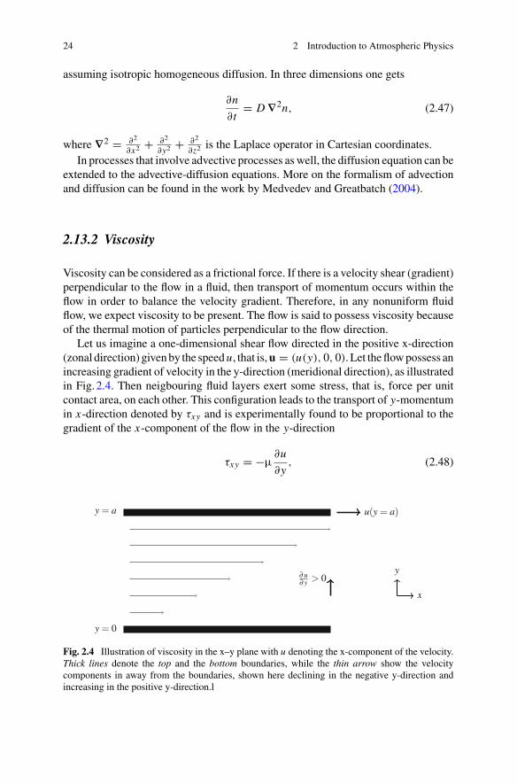
Let us imagine a one-dimensional shear flow directed in the positive x-direction(zonal direction) givenby the speedu, that is,u = (u(y), 0, 0). Let theflowpossess anincreasing gradient of velocity in the y-direction (meridional direction), as illustratedin Fig. 2.4. Then neigbouring fluid layers exert some stress, that is, force per unitcontact area, on each other. This configuration leads to the transport of y-momentumin x-direction denoted by τxy and is experimentally found to be proportional to thegradient of the x-component of the flow in the y-direction

τxy = −μ∂u

∂y, (2.48)

y= a u(y= a)

y= 0

y

x

∂ u∂ y > 0

Fig. 2.4 Illustration of viscosity in the x–y plane with u denoting the x-component of the velocity.Thick lines denote the top and the bottom boundaries, while the thin arrow show the velocitycomponents in away from the boundaries, shown here declining in the negative y-direction andincreasing in the positive y-direction.l

2.13 Transport Phenomena 25

where the proportionality factor μ is the coefficient of viscosity, which is given interms of the kinematic viscosity μ = ν ρ. In the absence of velocity shear there isno induced stress because of viscosity. In other words, the stress arising from thepresence of viscosity acting perpendicular to the flow is called shear stress. As theshear stress is proportional to the velocity gradient, the fluid said to be Newtonian.The physical significance of shear stresses in a fluid arises from the fact that anyimbalance in stress can lead to a net body force on the fluid. In our example, τxy

expresses the transfer of y-momentum in the x-direction, resulting from a veloc-ity shear in the y-direction. In a three-dimensional case, additional contribution tomomentum flux in x-direction can come from a velocity shear in the z-direction, thatis, τxz > 0 in the presence of shear in the z-direction. In general, the force per unitmass in the i-th direction resulting from viscous processes is

ai = Fi

m= 1

ρ

∂τi j

∂x j= − 1

ρ

∂

∂x j

(μ

∂ui

∂x j

), (2.49)

where τi j is the flux of x j -component ofmomentum in the xi -direction. It is importantto note that the total stressσi j arising in a fluid is composed of pressure (normal stress)and shear stress τi j

σi j = −pδi j + τi j , (2.50)

where δi j is the Kronecker delta with the property

δi j ={1 if i = j0 if i �= j

(2.51)

Viscous force arising from the relative motion of different fluid layers is always africtional force that counteracts the velocity variations in the flow.

2.13.3 Conduction

Conduction describes the flow of thermal energy per unit area per unit time, i.e.,heat flux. In response to a temperature gradient, heat is conducted. Heat flows in thedirection of decreasing temperature, that is, from hot to cold regions in accordancewith the second law of thermodynamics. In a uniform temperature distribution, heatconduction would be zero. Fourier’s law describes the heat conduction in a stationarymedium

q = −κ∂T

∂x, [J s−1 m−2] (2.52)

where q is heat flux, κ is the thermal conductivity, and T is temperature. Heat fluxdescribes the transfer of heat in terms of energy per unit area per unit time. Thenegative sign is because the heat flow is in the opposite direction to the temperature

26 2 Introduction to Atmospheric Physics

gradient. Fourier law of heat conduction assumes a steady-state heat conduction,meaning that the temperature distribution in the system is independent of time.

If we assume that the temperature distribution in a closed system is changingwith time, for example, due to time-varying boundary conditions, then we speak ofan unsteady (time-dependent) heat conduction process. The change of the internalenergy per unit mass ε is then

− ∂ε

∂t= 1

ρ

∂q

∂x= − ∂

∂x

(κ

∂T

∂x

). (2.53)

With ε = cvT and assuming constant thermal conductivity, we get the unsteady heatconduction equation

∂T

∂t= α

∂2T

∂x2. (2.54)

In three dimensions, we have

∂T

∂t= α ∇2T, (2.55)

where α = κ (ρ cv)−1 is the thermal diffusivity.

2.13.4 Radiation

Radiation is transport of energy (heat) by means of electromagnetic wave propaga-tion. Sun’s energy reaches us via radiation. Every matter in nature emits energy inform of radiation. The characteristics of the emission depends on the temperatureof the body. At higher temperatures higher frequency (shorter wavelength) emissiontakes place. Specifically, the rate of emission (energy radiation) associated with abody is proportional to the surface area A and to the fourth power of temperatureT 4. The Stefan-Boltzmann law is given by

dQ

dt= A εr σb T 4, [W] (2.56)

where dQ/dt is the heat flow, the proportionality constants εr is the radiative emis-sivity and σb = 5.67 × 10−8 W m−2 K−4 is the Stefan-Boltzmann constant. Theemissivity varies between 0 and 1 and is determined with respect to an ideal radiat-ing body with a given surface and at a given temperature. The net heat flow dependson the temperature difference between the emitting body and its surroundings. Forexample, the human body is about 10 ◦Cwarmer than the average room temperature.An emissivity of unity and body area of 1 m2 yield a net heat flow of about 60Wfrom the human body.

2.13 Transport Phenomena 27

The radiation field is described in terms of the amount of radiant energy dEν ina given frequency interval (ν, ν + dν), which is transported across an area elementdA in the direction confined to an element of the solid angle dω, during an timeinterval of dt (Chandrasekhar 1960). In terms of the intensity Iν associated with thefrequency ν, the infinitesimal radiant energy is expressed as

dEν = Iν cosα dA dω dν dt. (2.57)

Integration over all frequency bands yields the total radiant energy.

2.14 Richardson Number

The Richardson number Ri is a measure of evolution of turbulence in the atmosphereand describes atmospheric stability. It is given by

Ri = N 2

(∂u∂z

)2 + (∂v∂z

)2 , (2.58)

where N is the buoyancy frequency, u and v are the zonal andmeridional componentsof the horizontal flow, respectively. TheRichardson number expresses the importanceof vertical variations in a horizontal shear flow. If Ri > 0.25, the flow is stable, thatis, if the fluid is vertically displaced by a disturbance, it will either return to itsinitial position or perform pariodic oscillations around the equilibrium position. ForRi < 0.25, the flow undergoes dynamical instability and if the Ri < 0 then the flowis convectively instable. Another interpretation of Ri is as the ratio of productionof turbulence by buoyancy to the production of turbulence by wind shear (Nappo2002). Typically, dynamical instability preceeds convective instability. Horizontalflow with large wind shear is more prone to instability than the flow with small windshear.

2.15 Reynolds Number

The Reynolds number � is an important dimensionless parameter that characterizesthe nature of flow patterns in a fluid. It is defined as the ratio of inertial forces toviscous forces

� = ρ|u|Lμ

= uL

ν, (2.59)

where L is the length scale of the flow, ρ is the mass density, and μ is the viscositycoefficient (or dynamic viscosity). � can be used to identify whether the flow is

28 2 Introduction to Atmospheric Physics

laminar or turbulent. In a dynamic fluid � is variable. Increasing � means thatintertial effects are becoming gradually more dominant over viscous effect and theflow thus has a tendency to transition to a turbulent state.

References

Chandrasekhar S (1960) Radiative transfer. Dover books on physics, DoverMedvedev AS, Greatbatch RJ (2004) On advection and diffusion in the mesosphere and lower ther-mosphere: the role of rotational fluxes. J Geophys Res 109:D07104. doi:10.1029/2003JD003931

Nappo CJ (2002) An introduction to atmospheric gravity waves, International geophysics series,vol 85. Academic Press, Amsterdam

Yigit E, Ridley AJ (2011) Role of variability in determining the vertical wind speeds and structure.J Geophys Res 116:A12305. doi:10.1029/2011JA016714

http://www.springer.com/978-3-319-21580-8