Embed Size (px)
Citation preview

Ruprecht-Karls Universität HeidelbergKirchhoff-Institut für PhysikIm Neuenheimer Feld 22769120 Heidelberg
Atomic Force Microscopy
Instructions to the lab course
Last revised on January 7, 2014
Supervisors:
Jochen Vogt, KIP, room 2.301, phone 06221-549892e-mail: [email protected]
Michael Sendner, KIP, room 2.301, phone 06221-549892e-mail: [email protected]
Fabian Hötzel, KIP, room 2.208, phone 06221-549889e-mail: [email protected]
Olaf Skibbe, KIP, room 1.310, phone 06221-549890,e-mail: [email protected].
Location of practical course:KIP, INF 227, room 2.215

Preliminary Note
The aim of this practical course experiment is togive the students an insight into the technique ofscanning probe microscopy (SPM) with an atomicforce microscope (AFM) taken as example. Since thiskind of microscopy is widely-used in research areaswhich deal with structures on the nanometer scale, itmight serve as a prototypic example for an up-to-datemethod in surface science. At the same time the useddevice is sufficiently simple to be used by students inthe frame-set of a lab course without the permanentpresence of the supervisor.The students should be familiar with chapter 1
to 3 of this tutorial prior to the beginning of the
experiment. They should focus on the underlyingprinciples of the physics of the AFM. In additionto this instructions, a large variety of informationabout the subject and related methods is available forinstance in the world wide web. The list of questionsand tasks in the preparation section 2.3 should beanswered in advance to the lab course.Chapter 4 deals with the instrumental details for
the lab course and some additional information aboutproblem solving. This chapter is not necessary toread in advance.
This instructions are work in progress, so every hinton errors or on possible improvements is appreciated.
3
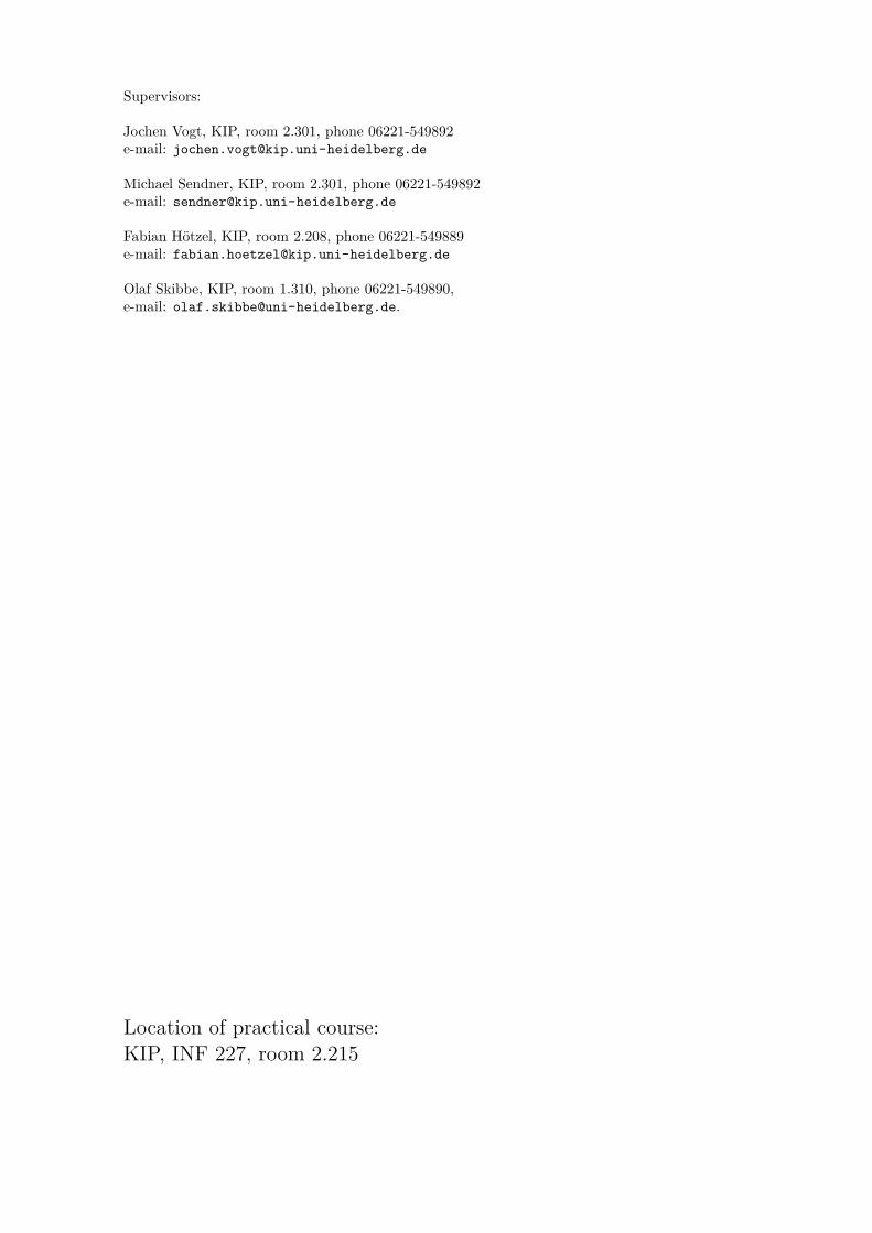
Contents
1 Introduction 51.1 Scanning Probe Microscopy . . . . . . . . . . . . . . . . . . . . . . . . . . . . . . . . . . . . 51.2 The Scanning Force Microscope . . . . . . . . . . . . . . . . . . . . . . . . . . . . . . . . . . 5
2 Basics 62.1 Theoretical Principles . . . . . . . . . . . . . . . . . . . . . . . . . . . . . . . . . . . . . . . 6
2.1.1 Van der Waals interaction . . . . . . . . . . . . . . . . . . . . . . . . . . . . . . . . . 62.1.2 Approaching the surface (Force distance behavior) . . . . . . . . . . . . . . . . . . . 72.1.3 Operation Modes . . . . . . . . . . . . . . . . . . . . . . . . . . . . . . . . . . . . . . 7
2.2 Operation Principles . . . . . . . . . . . . . . . . . . . . . . . . . . . . . . . . . . . . . . . . 92.2.1 Optics . . . . . . . . . . . . . . . . . . . . . . . . . . . . . . . . . . . . . . . . . . . . 92.2.2 Feedback control . . . . . . . . . . . . . . . . . . . . . . . . . . . . . . . . . . . . . . 9
2.3 Preparation Tasks . . . . . . . . . . . . . . . . . . . . . . . . . . . . . . . . . . . . . . . . . 10
3 Experiments and Evaluation 113.1 P and I Values . . . . . . . . . . . . . . . . . . . . . . . . . . . . . . . . . . . . . . . . . . . 113.2 Tip Characterisation and Limitations of the AFM . . . . . . . . . . . . . . . . . . . . . . . 113.3 Samples . . . . . . . . . . . . . . . . . . . . . . . . . . . . . . . . . . . . . . . . . . . . . . . 12
3.3.1 Pre-pressed and burned CD/DVD . . . . . . . . . . . . . . . . . . . . . . . . . . . . 123.3.2 Nano Lattice . . . . . . . . . . . . . . . . . . . . . . . . . . . . . . . . . . . . . . . . 123.3.3 CCD-Chip . . . . . . . . . . . . . . . . . . . . . . . . . . . . . . . . . . . . . . . . . . 123.3.4 Additional Samples . . . . . . . . . . . . . . . . . . . . . . . . . . . . . . . . . . . . . 12
3.4 Force-Distance Curve . . . . . . . . . . . . . . . . . . . . . . . . . . . . . . . . . . . . . . . . 12
4 Technical Support 154.1 Start-up . . . . . . . . . . . . . . . . . . . . . . . . . . . . . . . . . . . . . . . . . . . . . . . 154.2 Parameters for Image Mode . . . . . . . . . . . . . . . . . . . . . . . . . . . . . . . . . . . . 16
4.2.1 Scan Controls: . . . . . . . . . . . . . . . . . . . . . . . . . . . . . . . . . . . . . . . 164.2.2 Feedback Controls . . . . . . . . . . . . . . . . . . . . . . . . . . . . . . . . . . . . . 174.2.3 Channel 1, 2 and 3 . . . . . . . . . . . . . . . . . . . . . . . . . . . . . . . . . . . . . 17
4.3 Parameters for Force Mode . . . . . . . . . . . . . . . . . . . . . . . . . . . . . . . . . . . . 184.3.1 Main Control . . . . . . . . . . . . . . . . . . . . . . . . . . . . . . . . . . . . . . . . 184.3.2 Channel 1, 2 and 3 . . . . . . . . . . . . . . . . . . . . . . . . . . . . . . . . . . . . . 19
4.4 Trouble Shooting . . . . . . . . . . . . . . . . . . . . . . . . . . . . . . . . . . . . . . . . . . 194.5 Poor Image Quality . . . . . . . . . . . . . . . . . . . . . . . . . . . . . . . . . . . . . . . . 20
Bibliography 21
4
1 Introduction1.1 Scanning Probe MicroscopyThe method of scanning probe microscopy (SPM)was developed in 1981 by Binnig and Rohrer withthe invention of the scanning tunnelling microscope(STM) [1, 2]. This technique exploits the fact thata tunnelling current through a potential barrier ofthe width d is proportional to e−d (provided a con-stant and final height of the potential barrier). Witha sharp tip close to a surface, one can measure byapplying a voltage between tip and surface the tun-nelling current between the tip and the surface atomsin the vicinity of the tip. The strong dependence ofthe current from the distance d allows one to detectchanges in distance on a sub-atomic scale. By movingthe tip parallel to the surface, the height of the surfacecan be scanned. To control such distances, electro-mechanical devices of high precision are required.This task is commonly solved by piezo-ceramics. Foran understanding of the images generated this wayone has to take into account that the tunnelling cur-rent is also a function of the chemical properties ofthe surface. For a more detailed description anddiscussion of STM see e.g. [3, 4].
The scanning tunnelling microscope is (in general)restricted to conducting materials. The surfaces of in-sulators, structures in liquids and biological samplescan be imaged non destructive with high resolution bythe atomic force microscope (AFM) (also often scan-ning force microscope, SFM), which was developedin 1986 by Binnig, Quate and Gerber [5].
1.2 The Scanning ForceMicroscope
This subsections is mainly taken from [6] and slightlyadapted.
The design and development of the scanning forcemicroscope (SFM) (or frequently called atomic forcemicroscope AFM) is very closely connected with thatof scanning tunnelling microscopy. The central com-
ponent of these microscopes is basically the same. It isa fine tip positioned at a characteristic small distancefrom the sample. The height of the tip above thesample is adjusted by piezoelectric elements. In STMthe tunneling current gives the information aboutthe surface properties, whereas in SFM the forcesbetween the tip and the surface are used to gain thisinformation. The images are taken by scanning thesample relative to the probing tip and measuring thedeflection of the cantilever as a function of lateralposition. The height deflection is measured by opticaltechniques, which will be described in more detaillater.
A rich variety of forces can be sensed by scanningforce microscopy. In the non-contact mode (of dis-tances greater than 1 nm between the tip and thesample surface), van der Waals, electrostatic, mag-netic or capillary forces produce images, whereas inthe contact mode, repulsion forces take the leadingrole. Because its operation does not require a currentbetween the sample surface and the tip, the SFMcan move into potential regions inaccessible to thescanning tunnelling microscope (STM), for examplesamples which would be damaged irreparably by theSTM tunnelling current. Insulators, organic mate-rials, biological macromolecules, polymers, ceramicsand glasses are some of the many materials whichcan be imaged in different environments, such as inliquids, under vacuum, and at low temperatures.
In the non-contact mode one can obtain a surfaceanalysis with a true atomic resolution. However, inthis case the sample has to be prepared under ultra-high vacuum (UHV) conditions. Recently, it has beenshown that in the tapping mode (a modified non-contact mode) under ambient conditions it is possibleto observe, similar as in STM investigations, singlevacancies or their agglomeration [7]. Additionally, anon-contact mode has the further advantage over thecontact mode that the surface of very soft and roughmaterials is not influenced by frictional and adhesiveforces as during scanning in contact mode, i.e. thesurface is not “scratched”.
5
2 Basics
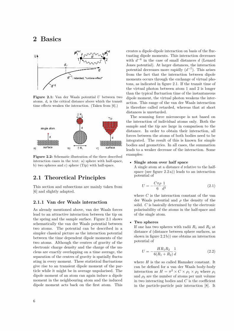
Figure 2.1: Van der Waals potential U between twoatoms. dr is the critical distance above which the transittime effects weaken the interaction. (Taken from [6].)
Figure 2.2: Schematic illustration of the three describedinteraction cases in the text: a) sphere with half-space,b) two spheres and c) sphere (Tip) with half-space.
2.1 Theoretical PrinciplesThis section and subsections are mainly taken from[6] and slightly adapted.
2.1.1 Van der Waals interactionAs already mentioned above, van der Waals forceslead to an attractive interaction between the tip onthe spring and the sample surface. Figure 2.1 showsschematically the van der Waals potential betweentwo atoms. The potential can be described in asimpler classical picture as the interaction potentialbetween the time dependent dipole moments of thetwo atoms. Although the centres of gravity of theelectronic charge density and the charge of the nu-cleus are exactly overlapping on a time average, theseparation of the centres of gravity is spatially fluctu-ating in every moment. These statistical fluctuationsgive rise to an transient dipole moment of the par-ticle while it might be in average unpolarised. Thedipole moment of an atom can again induce a dipolemoment in the neighbouring atom and the induceddipole moment acts back on the first atom. This
creates a dipole-dipole interaction on basis of the fluc-tuating dipole moments. This interaction decreaseswith d−6 in the case of small distances d (LenardJones potential). At larger distances, the interactionpotential decreases more rapidly (d−7). This arisesfrom the fact that the interaction between dipolemoments occurs through the exchange of virtual pho-tons, as indicated in figure 2.1. If the transit time ofthe virtual photon between atom 1 and 2 is longerthan the typical fluctuation time of the instantaneousdipole moment, the virtual photon weakens the inter-action. This range of the van der Waals interactionis therefore called retarded, whereas that at shortdistances is unretarded.The scanning force microscope is not based on
the interaction of individual atoms only. Both thesample and the tip are large in comparison to thedistance. In order to obtain their interaction, allforces between the atoms of both bodies need to beintegrated. The result of this is known for simplebodies and geometries. In all cases, the summationleads to a weaker decrease of the interaction. Someexamples:
• Single atom over half spaceA single atom at a distance d relative to the half-space (see figure 2.2 a)) leads to an interactionpotential of
U = −Cπρ61d3 (2.1)
where C is the interaction constant of the vander Waals potential and ρ the density of thesolid. C is basically determined by the electronicpolarisability of the atoms in the half-space andof the single atom.
• Two spheresIf one has two spheres with radii R1 and R2 atdistance d (distance between sphere surfaces, asshown in figure 2.2 b)) one obtains an interactionpotential of
U = − HR1R2
6(R1 +R2)1d
(2.2)
where H is the so called Hamaker constant. Itcan be defined for a van der Waals body-bodyinteraction as H = π2 × C × ρ1 × ρ2 where ρ1and ρ2 are the number of atoms per unit volumein two interacting bodies and C is the coefficientin the particle-particle pair interaction [8]. It
6
2.1 Theoretical Principles
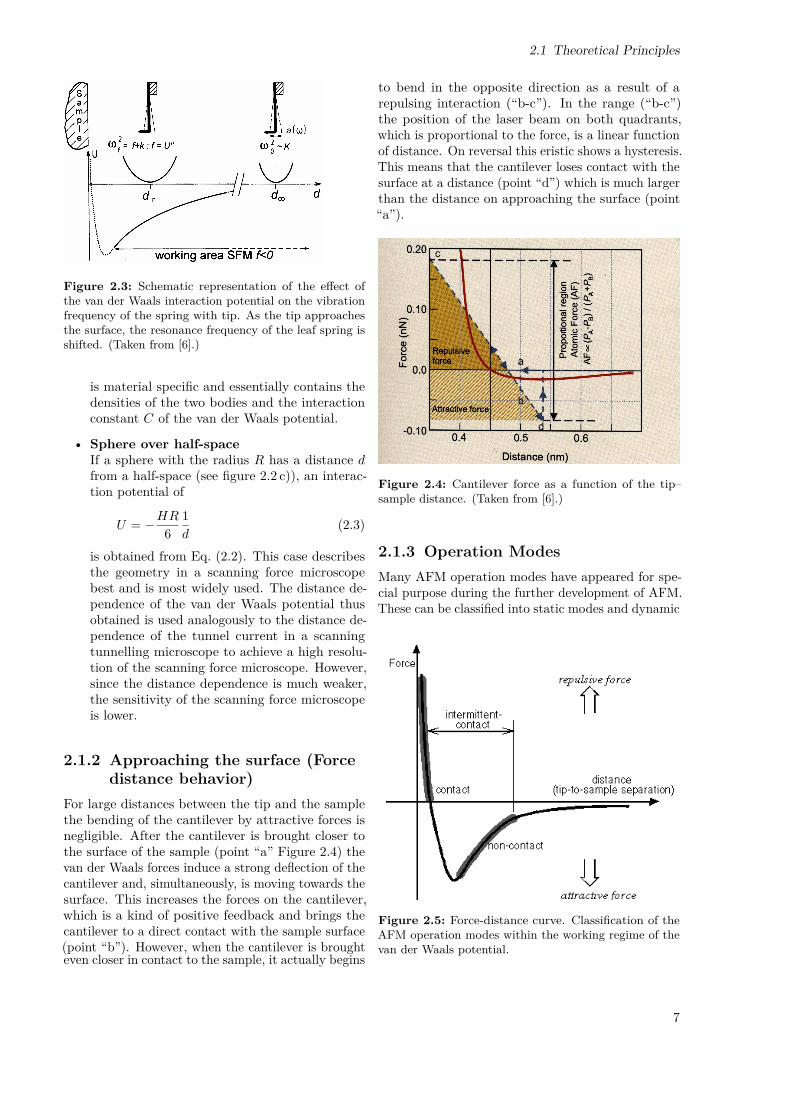
Figure 2.3: Schematic representation of the effect ofthe van der Waals interaction potential on the vibrationfrequency of the spring with tip. As the tip approachesthe surface, the resonance frequency of the leaf spring isshifted. (Taken from [6].)
is material specific and essentially contains thedensities of the two bodies and the interactionconstant C of the van der Waals potential.
• Sphere over half-spaceIf a sphere with the radius R has a distance dfrom a half-space (see figure 2.2 c)), an interac-tion potential of
U = −HR61d
(2.3)
is obtained from Eq. (2.2). This case describesthe geometry in a scanning force microscopebest and is most widely used. The distance de-pendence of the van der Waals potential thusobtained is used analogously to the distance de-pendence of the tunnel current in a scanningtunnelling microscope to achieve a high resolu-tion of the scanning force microscope. However,since the distance dependence is much weaker,the sensitivity of the scanning force microscopeis lower.
2.1.2 Approaching the surface (Forcedistance behavior)
For large distances between the tip and the samplethe bending of the cantilever by attractive forces isnegligible. After the cantilever is brought closer tothe surface of the sample (point “a” Figure 2.4) thevan der Waals forces induce a strong deflection of thecantilever and, simultaneously, is moving towards thesurface. This increases the forces on the cantilever,which is a kind of positive feedback and brings thecantilever to a direct contact with the sample surface(point “b”). However, when the cantilever is broughteven closer in contact to the sample, it actually begins
to bend in the opposite direction as a result of arepulsing interaction (“b-c”). In the range (“b-c”)the position of the laser beam on both quadrants,which is proportional to the force, is a linear functionof distance. On reversal this eristic shows a hysteresis.This means that the cantilever loses contact with thesurface at a distance (point “d”) which is much largerthan the distance on approaching the surface (point“a”).
Figure 2.4: Cantilever force as a function of the tip–sample distance. (Taken from [6].)
2.1.3 Operation ModesMany AFM operation modes have appeared for spe-cial purpose during the further development of AFM.These can be classified into static modes and dynamic
Figure 2.5: Force-distance curve. Classification of theAFM operation modes within the working regime of thevan der Waals potential.
7

2 Basics
Figure 2.6: Resonance curves of the tip without andwith a van der Waals potential. The interaction leads to ashift ∆ω of the resonance frequency with the consequencethat the tip excited with the frequency ωm has a vibrationamplitude a(ω) attenuated by ∆a. (Taken from [6].)
modes. Another classification could be contact, non-contact and intermittent-contact which is reclined tothe working regimes (see figure 2.5).
Here the three commonly used techniques, namelystatic mode (contact mode) and dynamic mode (non-contact mode and tapping mode) will be shortly de-scribed. Further information can be found in text-books or review articles.
Contact mode/static mode
In contact mode the tip scans the sample in closecontact with the surface and the force acting on thetip is repulsive of the order of 10−9N. This scanningmode is very fast, but has the disadvantage that ad-ditionally to the normal force frictional forces appearwhich can be destructive and damage the sampleor/and the tip.
Constant height mode: This mode is particularsuited for very flat samples. The height of the tipis set constant and by scanning the sample only thedeflection of the cantilever is detected by an opticalsystem (described in 2.2.1) and gives the topographicinformation.
Constant force mode: In this mode the force act-ing on the cantilever, i.e. the deflection, is set to acertain value and changes in deflection can be used asinput for the feedback circuit that moves the scannerup and down. The system is therefore respondingto the changes in height by keeping the cantileverdeflection constant. The motion of the scanner givesthe direct information about the topography of thesample. The scanning time is limited by the response
of the feedback circuit and therefore not as fast asthe constant height mode.
Dynamic Modes
The dynamic operation method of a scanning forcemicroscope has proved to be particularly useful. Inthis method the normal force constant of the van derWaals potential, i.e. the second derivative of the po-tential, is exploited. This can be measured by usinga vibrating tip (Figure 2.3). If a tip vibrates at a dis-tance d, which is outside the interaction range of thevan der Waals potential, then the vibration frequencyand the amplitude are only determined by the springconstant k of the cantilever. This corresponds to aharmonic potential. When the tip comes into theinteraction range of the van der Waals potential, theharmonic potential and the interaction potential aresuperimposed thus changing the vibration frequencyand the amplitude of the spring.
This is described by modifying the spring constantk of the spring by an additional contribution f ofthe van der Waals potential. As a consequence, thevibration frequency is shifted to lower frequencies asshown in Figure 2.6. ω0 is the resonance frequencywithout interaction and ∆ω is the frequency shift tolower values. If an excitation frequency of the tip ofωm > ω0 is selected and kept constant, the ampli-tude of the vibration decreases as the tip approachesthe sample, since the interaction becomes increas-ingly stronger. Thus, the vibration amplitude alsobecomes a measure for the distance of the tip fromthe sample surface. If a spring with a low dampingQ−1 is selected, the resonance curve is steep and theratio of the amplitude change for a given frequencyshift becomes large. In practice, small amplitudes(approx. 1 nm) in comparison to distance d are usedto ensure the linearity of the amplitude signal. Witha given measurement accuracy of 1 %, however, thismeans the assembly must measure deflection changesof 0.001 nm, which is achieved most simply by a laserinterferometer or optical lever method.
Non-contact mode: Since in the non-contactregime the force between the tip and the surfaceis of the order of 10−12 N and therefore much weakerthan in the contact regime the tip has to be driven inthe dynamic mode, i.e. the tip is vibrated near thesurface of the sample and changes in resonance fre-quency or amplitude are detected and used as inputfor the feedback circuit. In this case the resonancefrequency or the amplitude are held constant by mov-ing the sample up and down and recording directlythe topography of the sample.
8
2.2 Operation Principles
Tapping mode: Tapping mode is an intermittent-contact mode. In general it is similar to the non-contact mode described before, except that the tip isbrought closer to the surface and taps the surface atthe end of his oscillation. This mode is much moresensitive than the non-contact mode and in contraryto contact mode no frictional forces appear whichcan alter the tip or the surface. Therefore this is themode of choice for the most experiments and duringthe lab course.
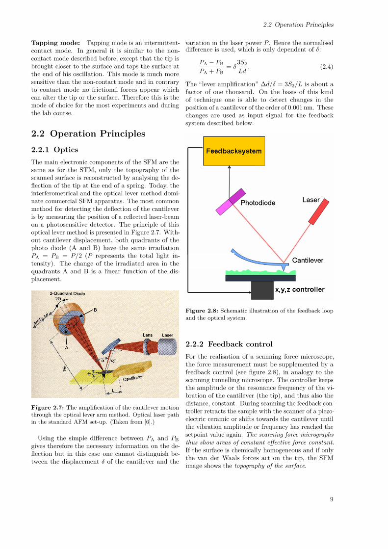
2.2 Operation Principles2.2.1 OpticsThe main electronic components of the SFM are thesame as for the STM, only the topography of thescanned surface is reconstructed by analysing the de-flection of the tip at the end of a spring. Today, theinterferometrical and the optical lever method domi-nate commercial SFM apparatus. The most commonmethod for detecting the deflection of the cantileveris by measuring the position of a reflected laser-beamon a photosensitive detector. The principle of thisoptical lever method is presented in Figure 2.7. With-out cantilever displacement, both quadrants of thephoto diode (A and B) have the same irradiationPA = PB = P/2 (P represents the total light in-tensity). The change of the irradiated area in thequadrants A and B is a linear function of the dis-placement.
Figure 2.7: The amplification of the cantilever motionthrough the optical lever arm method. Optical laser pathin the standard AFM set-up. (Taken from [6].)
Using the simple difference between PA and PBgives therefore the necessary information on the de-flection but in this case one cannot distinguish be-tween the displacement δ of the cantilever and the
variation in the laser power P . Hence the normaliseddifference is used, which is only dependent of δ:
PA − PB
PA + PB= δ
3S2
Ld. (2.4)
The “lever amplification” ∆d/δ = 3S2/L is about afactor of one thousand. On the basis of this kindof technique one is able to detect changes in theposition of a cantilever of the order of 0.001 nm. Thesechanges are used as input signal for the feedbacksystem described below.
Figure 2.8: Schematic illustration of the feedback loopand the optical system.
2.2.2 Feedback controlFor the realisation of a scanning force microscope,the force measurement must be supplemented by afeedback control (see figure 2.8), in analogy to thescanning tunnelling microscope. The controller keepsthe amplitude or the resonance frequency of the vi-bration of the cantilever (the tip), and thus also thedistance, constant. During scanning the feedback con-troller retracts the sample with the scanner of a piezo-electric ceramic or shifts towards the cantilever untilthe vibration amplitude or frequency has reached thesetpoint value again. The scanning force micrographsthus show areas of constant effective force constant.If the surface is chemically homogeneous and if onlythe van der Waals forces act on the tip, the SFMimage shows the topography of the surface.
9

2 Basics
2.3 Preparation Tasks• What are the underlying principles of AFM?
What forces act between tip and sample? Whatdoes the corresponding potential look like?
• Briefly describe the experimental setup of theAFM. How is the information on the sampletopography obtained?
• What operation modes can be chosen? Brieflydescribe the different modes and their advan-tages/disadvantages.
• During this lab course we will only use the tap-ping mode. How does this mode work in detail?(How is the resonance curve (amplitude vs. fre-quency) modified when the tip approaches thesurface? Which parameter of the oscillation pro-vides information on the height profile when theexcitation frequency is kept constant?
• In our case the system keeps the distance betweentip and sample surface constant. This is done
by piezo-materials and a PID controller. Howcan piezo-materials be used in motion systems?What is a PID controller?
• What’s the resolution of an AFM and how is itlimited? How is the image influenced by the tipshape?
• What are the advantages of an AFM? E.g. incomparison with a SEM or STM?
• Get information from the internet on how thedata is stored on a CD (How are 0 and 1 real-ized? How is the data stored? Keyword: Eight-to-Fourteen-Modulation). You can find a niceoverview at: http://rz-home.de/~drhubrich/CD.htm#code
• In the last part of the lab course a force-distancecurve will be measured. How does the deflectionof the tip (proportional to the force) change whenit approaches the surface? What difference doyou expect for retracting the tip?
10
3 Experiments and Evaluation
Goal of these experiments is to learn about thebasic functioning and possibilities of the atomic forcemicroscope. The structure of two calibration gridsand different surfaces will be observed and quantified.A detailed description on how to operate the mi-
croscope and the meaning of the different scan pa-rameters is given in chapter 4. It is essential thatthe correct profile (afmprak2) is loaded. In case ofproblems, have a look at sections 4.1 and 4.4.
Important: All measurements for the wholelab course should be performed with the maxi-mum resolution of 512 x 512 points and a scanrate of 1 Hz.
It takes quite some time to record an AFM imagebut you can and you should use this time to do yourevaluation.
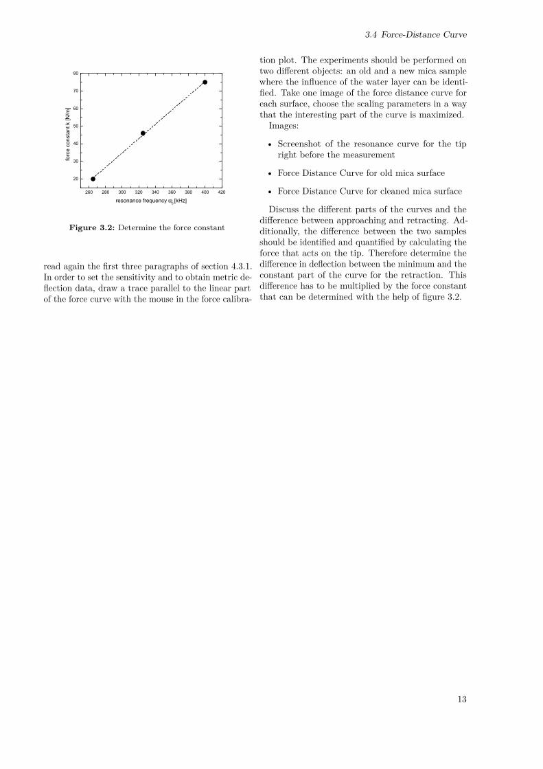
3.1 P and I ValuesStart the microscope as described in chapter 4.1 andtake a screenshot of the resonance curve. As firstsample use the calibration grid TGZ02 (see figure3.3).
Vary the values of the proportional gain P andthe integral gain I, while imaging the surface of thecalibration grid in Dual Trace Mode. Try to findoptimal values for both parameters. Take pictures forthe optimal values you found and for too high andtoo low values for I, respectively.Images that have to be taken:• Screenshot of the resonance curve (old tip)
• Dual Trace Mode for optimal P and I values
• Dual Trace Mode for too high I values
• Dual Trace Mode for too low I valuesDiscuss the effect of high/low proportional and inte-gral gain with respect to the image quality versus areliable height measurement.
Important: The P and I values have tobe checked and potentially adjusted for everynew sample.
3.2 Tip Characterisation andLimitations of the AFM
In order to experience the limitations of the AFMtwo calibration grids with different step heights are
measured.Important: All measurements for the
whole lab course should be performed witha resolution of 512 x 512 points and a scanrate of 1 Hz.Start with calibration grid TGZ02 and take one
image with the scanning direction perpendicular tothe steps, then change the scanning angle about 90◦
and take a second image with scanning directionparallel to the steps. Describe what you observefor the different scanning directions and discuss thereason for your observation.Repeat the measurement with scanning direction
perpendicular to the steps for the calibration gridTGZ01 (don’t forget to readjust the P and I values).After you finished all measurements with the oldtip, determine again the resonance curve and take ascreenshot.After that a new tip will be given to you by your
supervisor. First take a screenshot of the new res-onance curve and then investigate again the gridTGZ01 (perpendicular scanning direction).
All images that have to be taken for this part ofthe lab course are listed below:
• TGZ02 scanning direction perpendicular to thesteps (10µm x 10µm) (old tip)
• TGZ02 scanning direction parallel to the steps(10µm x 10µm) (old tip)
• TGZ01 scanning direction perpendicular to thesteps (10µm x 10µm) (old tip)
• Screenshot of the resonance curve (old tip)
• Screenshot of the resonance curve (new tip)
• TGZ01 scanning direction perpendicular to thesteps (10µm x 10µm) (new tip)
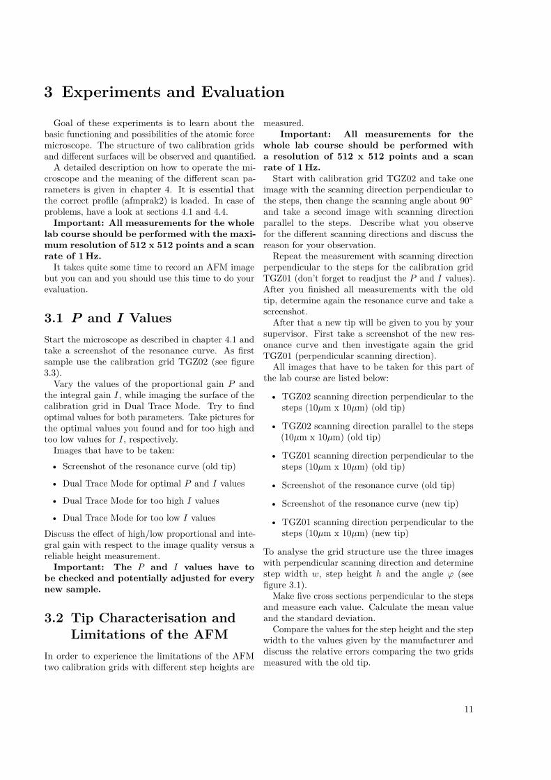
To analyse the grid structure use the three imageswith perpendicular scanning direction and determinestep width w, step height h and the angle ϕ (seefigure 3.1).
Make five cross sections perpendicular to the stepsand measure each value. Calculate the mean valueand the standard deviation.
Compare the values for the step height and the stepwidth to the values given by the manufacturer anddiscuss the relative errors comparing the two gridsmeasured with the old tip.
11
3 Experiments and Evaluation
h
w
φ
Figure 3.1: Values to be determined in the evaluation
Second, compare the values obtained for TGZ01with the new and the old tip. Discuss these resultsin terms of tip radius, shape and inclination.In addition compare the resonance curves with
respect to the shape and the resonance position, useas well the resonance curve determined in 3.1. Arethere any changes/differences?
3.3 Samples3.3.1 Pre-pressed and burned
CD/DVDIn order to estimate the capacity of a CD, a sampleof a pre-pressed CD-ROM has been prepaired wet-chemically for you. Take an overview image (10µm x10µm), think about the best scanning direction (par-allel or perpendicular to the spiral lines) to determinethe length of a pit.
• Pre-pressed CD surface with best scanning di-rection (10µm x 10µm)
Measure (with a ruler) the area of the CD wheredata is stored. From this area you can calculate thelength of the total track using the distance betweentwo spiral lines. Determine the length of the shortestpit and compare this to literature data. How is thedigital information (1 and 0) stored on a CD andhow many channelbits are coded in the shortest pit?Furthermore, try to estimate the capacity of a CDusing your results. (This might be helpful: http://rz-home.de/~drhubrich/CD.htm#Code)
Now prepare a sample of a burned CD surface onyour own by retracting a small square of the dye layer.Again take an overview image (10µm x 10µm).
• Burned CD surface with best scanning direction(10µm x 10µm)
What are the differences between the two samples(only qualitatively)? What are the reasons for that?
3.3.2 Nano LatticeThe areas with the nano lattices are visible withbare eye as rainbow-coloured stripes when reflecting
light on the sample. In the optical microscope thecolors are not clearly visible but there are bright anddark stripes. The geometric properties of the stripeschange continously from the dark to the bright side.Determine to which end of the rainbow the dark andthe bright stripes correspond respectively. Choosetwo different stripes (one from the dark and one fromthe bright side) and take one image of each.Images:
• Stripe from dark side (approx. 1.5µm x 1.5µm)
• Stripe from bright side (approx. 1.5µm x 1.5µm)
Characterize the structures you find (depths, diam-eter, distance between features) and compare thevalues obtained for the two different stripes. Howdo the geometric dimensions correlate to the colorimpression?Imagine the lattice you observed being smaller
(with a lattice constant of a few Ångstrom) and thelattice points being occupied by atoms of the samespecies. Which surface of an fcc crystal is then rep-resented? Hint: Try to remember how the low-indexsurfaces fcc(100), fcc(110) and fcc(111) look like!
3.3.3 CCD-ChipImportant: The CCD-chip is a very high sam-ple. Make sure you raise the AFM tip highenough before changing the sample!
This sample is the CCD-chip of an old digital cam-era. Take an image of the surface.
• CCD-Chip (10µm x 10µm)
Measure (with a ruler) the size of the whole chip. De-termine the size of one pixel from your measurement.Calculate the megapixels of this camera. When youdo this, remember that the camera can take colorpictures! How is the color information obtained?
3.3.4 Additional SamplesYou are encouraged to bring along some samples ofyour own. The size of the samples should not exceed10 mm×10 mm×4 mm and the structures should notbe higher than 500 nm.
3.4 Force-Distance CurveUse a mica surface to get a force-distance curve forapproaching and retracting the surface. First youdetermine again the resonance curve for the tip youare currently using. Then start imaging the surfacein tapping mode and switch during acquisition intothe force-distance curve mode. Before you do that
12
3.4 Force-Distance Curve
2 6 0 2 8 0 3 0 0 3 2 0 3 4 0 3 6 0 3 8 0 4 0 0 4 2 0
2 0
3 0
4 0
5 0
6 0
7 0
8 0for
ce co
nstan
t k [N
/m]
r e s o n a n c e f r e q u e n c y ω0 [ k H z ]
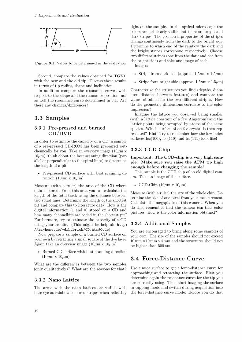
Figure 3.2: Determine the force constant
read again the first three paragraphs of section 4.3.1.In order to set the sensitivity and to obtain metric de-flection data, draw a trace parallel to the linear partof the force curve with the mouse in the force calibra-
tion plot. The experiments should be performed ontwo different objects: an old and a new mica samplewhere the influence of the water layer can be identi-fied. Take one image of the force distance curve foreach surface, choose the scaling parameters in a waythat the interesting part of the curve is maximized.Images:
• Screenshot of the resonance curve for the tipright before the measurement
• Force Distance Curve for old mica surface
• Force Distance Curve for cleaned mica surface
Discuss the different parts of the curves and thedifference between approaching and retracting. Ad-ditionally, the difference between the two samplesshould be identified and quantified by calculating theforce that acts on the tip. Therefore determine thedifference in deflection between the minimum and theconstant part of the curve for the retraction. Thisdifference has to be multiplied by the force constantthat can be determined with the help of figure 3.2.
13
3 Experiments and Evaluation
Figure 3.3: Data sheet for calibration grid TGZ01-TGZ02
14
4 Technical Support
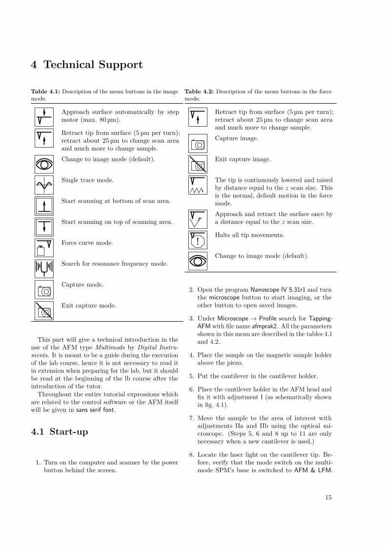
Table 4.1: Description of the menu buttons in the imagemode.
Approach surface automatically by stepmotor (max. 80 µm).
Retract tip from surface (5 µm per turn);retract about 25 µm to change scan areaand much more to change sample.Change to image mode (default).
Single trace mode.
Start scanning at bottom of scan area.
Start scanning on top of scanning area.
Force curve mode.
Search for resonance frequency mode.
Capture mode.
Exit capture mode.
This part will give a technical introduction in theuse of the AFM type Multimode by Digital Instru-ments. It is meant to be a guide during the executionof the lab course, hence it is not necessary to read itin extension when preparing for the lab, but it shouldbe read at the beginning of the lb course after theintroduction of the tutor.Throughout the entire tutorial expressions which
are related to the control software or the AFM itselfwill be given in sans serif font.
4.1 Start-up
1. Turn on the computer and scanner by the powerbutton behind the screen.
Table 4.2: Description of the menu buttons in the forcemode.
Retract tip from surface (5 µm per turn);retract about 25 µm to change scan areaand much more to change sample.Capture image.
Exit capture image.
The tip is continuously lowered and raisedby distance equal to the z scan size. Thisis the normal, default motion in the forcemode.Approach and retract the surface once bya distance equal to the z scan size.
!Halts all tip movements.
Change to image mode (default).
2. Open the program Nanoscope IV 5.31r1 and turnthe microscope button to start imaging, or theother button to open saved images.
3. Under Microscope → Profile search for Tapping-AFM with file name afmprak2. All the parametersshown in this menu are described in the tables 4.1and 4.2.
4. Place the sample on the magnetic sample holderabove the piezo.
5. Put the cantilever in the cantilever holder.
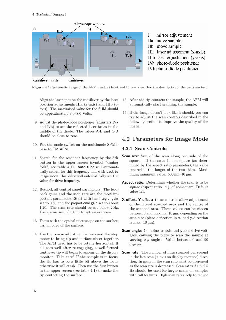
6. Place the cantilever holder in the AFM head andfix it with adjustment I (as schematically shownin fig. 4.1).
7. Move the sample to the area of interest withadjustments IIa and IIb using the optical mi-croscope. (Steps 5, 6 and 8 up to 11 are onlynecessary when a new cantilever is used.)
8. Locate the laser light on the cantilever tip. Be-fore, verify that the mode switch on the multi-mode SPM’s base is switched to AFM & LFM.
15
4 Technical Support
Figure 4.1: Schematic image of the AFM head, a) front and b) rear view. For the description of the parts see text.
Align the laser spot on the cantilever by the laserposition adjustments IIIa (x-axis) and IIIb (y-axis). The maximised value for the SUM shouldbe approximately 3.0–8.0 Volts.
9. Adjust the photo-diode positioner (adjusters IVaand Ivb) to set the reflected laser beam in themiddle of the diode. The values A-B and C-Dshould be close to zero.
10. Put the mode switch on the multimode SPM’sbase to TM AFM.
11. Search for the resonant frequency by the 8thbutton in the upper screen (symbol “tuningfork”, see table 4.1). Auto tune will automat-ically search for this frequency and with back toimage mode, this value will automatically set thevalue for drive frequency.
12. Recheck all control panel parameters. The feed-back gains and the scan rate are the most im-portant parameters. Start with the integral gainset to 0.50 and the proportional gain set to about1.20. The scan rate should be set below 2Hz.Use a scan size of 10 µm to get an overview.
13. Focus with the optical microscope on the surface,e.g. an edge of the surface.
14. Use the coarse adjustment screws and the stepmotor to bring tip and surface closer together.The AFM head has to be totally horizontal. Ifall goes well after re-engaging, a well-formedcantilever tip will begin to appear on the displaymonitor. Take care! If the sample is in focus,the tip has to be a little bit above the focusotherwise it will crash. Then use the first buttonin the upper screen (see table 4.1) to make thetip contacting the surface.
15. After the tip contacts the sample, the AFM willautomatically start scanning the sample.
16. If the image doesn’t look like it should, you cantry to adjust the scan controls described in thefollowing section to improve the quality of theimage.
4.2 Parameters for Image Mode4.2.1 Scan Controls:Scan size: Size of the scan along one side of the
square. If the scan is non-square (as deter-mined by the aspect ratio parameter), the valueentered is the longer of the two sides. Maxi-mum/minimum value: 500 nm–10 µm.
Aspect ratio: Determines whether the scan is to besquare (aspect ratio 1:1), of non-square. Defaultvalue 1:1.
X offset, Y offset: these controls allow adjustmentof the lateral scanned area and the centre ofthe scanned area. These values can be chosenbetween 0 and maximal 10 µm, depending on thescan size (piezo deflection in x- and y-directionis max. 10 µm).
Scan angle: Combines x-axis and y-axis drive volt-ages, causing the piezo to scan the sample atvarying x-y angles. Value between 0 and 90degrees.
Scan rate: The number of lines scanned per secondin the fast scan (x-axis on display monitor) direc-tion. In general, the scan rate must be decreasedas the scan size is decreased. Scan rates if 1.5–2.5Hz should be used for larger scans on sampleswith tall features. High scan rates help to reduce
16
4.2 Parameters for Image Mode
drift, but they can only be used on very flat sam-ples with small scan sizes. Maximum/minimumvalue: 0.1–5Hz.
Tip velocity: The scanned distance per second inthe fast scan direction (changes as the scan ratechanges).
Samples/line: Number of imaged points per scannedline. Maximum/minimum value: 128–1024 (de-fault value 512).
Lines: number of scanned lines. This value is thesame as samples/line for aspect ratio of 1:1. Max-imum/minimum value: 128–1024; default value512.
Number of samples: Sets the number of pixels dis-played per line and the number of lines perscanned frame.
Slow scan axis: Starts and stops the slow scan (y-axis on display monitor). This control is used toallow the user to check for lateral mechanical driftin the microscope or assist in tuning the feedbackgains. Always set to enable unless checking fordrift or tuning gains. Default value: enable.
4.2.2 Feedback ControlsSPM feedback: Sets the signal used as feedback in-
put. Possible signals are Amplitude (default), TMdeflection and Phase.
Integral gain and proportional gain: Controls theresponse time of the feedback loop. The feedbackloop tries to keep the output of the SPM equalto the setpoint reference chosen. It does this bymoving the piezo in z to keep the SPM’s outputon track with the setpoint reference. Piezoelec-tric transducers have a characteristic responsetime to the feedback voltage applied. The gainsare simply values that magnify the differenceread at the A/D converter. This causes the com-puter to think that the SPM output is furtheraway from the setpoint reference than it reallyis. The computer essentially overcompensatesfor this by sending a larger voltage to the zpiezo than it truly needed. This causes the piezoscanner to move faster in z. This is done tocompensate for the mechanical hysteresis of thepiezo element. The effect is smoothed out dueto the fact that the piezo is adjusted up to fourtimes the rate of the display rate. Optimise theintegral gain and proportional gain so that theheight image shows the sharpest contrast andthere are minimal variations in the amplitudeimage (the error signal). It may be helpful to
optimise the scan rate to get the sharpest im-age. Maximum/minimum value for integral gain:0.1–4 and for proportional gain: 0.1–10. Defaultvalues between 2 and 3.
Amplitude setpoint: The setpoint defines the de-sired voltage for the feedback loop. The setpointvoltage is constantly compared to the presentRMS amplitude voltage to calculate the desiredchange in the piezo position. When the SPMfeedback is set to amplitude, the z piezo positionchanges to keep the amplitude voltage close tothe setpoint; therefore, the vibration amplituderemains nearly constant. Changing the setpointalters the response of the cantilever vibrationand changes the amount of force applied to thesample. Maximum/minimum value: 1–8.
Drive frequency: Defines the frequency at which thecantilever is oscillated. This frequency shouldbe very close to the resonant frequency of thecantilever. These value is around 300 kHz for thecantilevers used.
Drive amplitude: Defines the amplitude of the volt-age applied to the piezo system that drives thecantilever vibration. It is possible to fracturethe cantilever by using too high drive amplitude;therefore, it is safer to start with a small valueand increase the value incrementally. If the am-plitude calibration plot consist of a flat line allthe way across, changing the value of this pa-rameter should shift the level of the curve. Ifit does not, the tip is probably fully extendedinto the surface and the tip should be withdrawnbefore proceeding. Maximum/minimum value:10–60mV, default 30 mV.
4.2.3 Channel 1, 2 and 3Data type: Height data corresponds to the change
in piezo height needed to keep the vibrationalamplitude of the cantilever constant. Ampli-tude data describes the change in the amplitudedirectly. Deflection data comes from the differen-tial signal off of the top and bottom photo-diodesegments.
Data scale: This parameter controls the verticalscale corresponding to the full height of the dis-play and colour bar.
Data centre: Offsets the centreline on the colourscale by the amount entered.
Line direction: Selects the direction of the fast scanduring data collection. Only one-way scanningis possible.Range of settings:
17

4 Technical Support
• Trace: Data is collected when the relativemotion of the tip is left to right as viewedfrom the front of the microscope.
• Retrace: Data is collected when the relativetip motion is right to left as viewed fromthe front of the microscope.
Scan line: The scan line controls whether data fromthe Main of Interleave scan line is displayed andcaptured.
Real-time plane fit: Applies a software leveling planeto each real-time image, thus removing up to first-order tilt. Five types of plane-fit are availableto each real-time image shown on the displaymonitor.Range of settings:
• None: Only raw, unprocessed data is dis-played.
• Offset: Takes the z-axis average of eachscan line, then subtracts it from every datapoint.
• Line: Takes the slope and z-axis average ofeach scan line and subtracts it from eachdata point in that scan line. This is thedefault mode of operation, and should beused unless there is a specific reason to dootherwise.
• AC: Takes the slope and z-axis average ofeach scan line across one-half of that line,then subtracts it from each data point inthat scan line.
• Frame: Level the real-time image based ona best-fit plane calculated from the mostrecent real-time frame performed with thesame frame direction (up or down).
• Captured: Level the real-time image basedon a best fit plane calculated from a planecaptured with the capture plane commandin.
Off line plane fit: Applies a software levelling planeto each off-line image for removing first-ordertilt. Five types of plane-fit are available to eachoff-line image.Range of settings:
• None: Only raw, unprocessed data is dis-played.
• Offset: Captured images have a DC z offsetremoved from them, but they are not fittedto a plane.
• Full: A best-fit plane that is derived fromthe data file is subtracted from the capturedimage.
High-pass filter: This filter parameter invokes a dig-ital, two-pole, high-pass filter that removes lowfrequency effects, such as ripples caused by tor-sional forces on the cantilever when the scanreverses direction. It operates on the digitaldata stream regardless of scan direction. Thisparameter can be off or set from 0 through 9.Settings of 1 through 9, successively, lower thecut-off frequency of the filter applied to the datastream. It is important to realize that in remov-ing low frequency information from the image,the high-pass filter distorts the height informa-tion in the image.
Low-pass filter: This filter invokes a digital, one-pole, low-pass filter to remove high-frequencynoise from the Real Time data. The filter oper-ates on the collected digital data regardless ofthe scan direction. Settings for this item rangefrom off through 9. Off implies no low-pass fil-tering of the data, while settings of 1 through 9,successively, lower the cut-off frequency of thefilter applied to the data stream.
4.3 Parameters for Force Mode4.3.1 Main ControlRamp channel: Defines the variable to be plotted
along the x-axis of the scope trace. Default Z.
Ramp size: This parameter defines the total traveldistance of the piezo. Use caution when workingin the force mode. This mode can potentiallydamage the tip and/or surface by too high valuesfor the ramp size.
Z scan start: This parameter sets the offset of thepiezo travel (i.e., its starting point). It sets themaximum voltage applied to the z electrodes ofthe piezo during the force plot operation. Thetriangular waveform is offset up and down in re-lation to the value of this parameter. Increasingthe value of the z scan start parameter moves thesample closer to the tip by extending the piezotube.
Scan rate: sets the rate with which the z-piezo ap-proach/retract the tip. Maximum/minimumvalue: 0.1–5Hz.
X offset and Y offset: controls the centre positionof the scan in the x- and y- directions, respec-tively; same as in image mode. Range of settings:±220 V.
Number of samples: Defines the number of datapoints captured during each extension/retraction
18

4.4 Trouble Shooting
cycle of the z-piezo. Maximum/minimum value:128–1024; default value 512.
Average count: sets the number of scans taken toaverage the display of the force plot. May be setbetween 1 and 1024. Usually it is set to 1 unlessthe user needs to reduce noise.
Spring constant: This parameter relates the can-tilever deflection signal to the z travel of thepiezo. It equals the slope of the deflection versusz when the tip is in contact with the sample. Fora proper force curve, the line has a negative slopewith typical values of 10–50mV/nm; however,by convention, values are shown as positive inthe menu.
Display mode: The portion of a tip’s vertical motionto be plotted on the force graph.Range of settings:
• Extend: Plots only the extension portion ofthe tip’s vertical travel.
• Retract: Plots only the retraction portionof the tip’s vertical travel.
• Both: Plots both the extension and retrac-tion portion of the tip’s vertical travel.
Units: This item selects the units of the parameters,either metric lengths or volts.
X rotate: allows the user to move the tip laterally,in the x-direction, during indentation. This isuseful since the cantilever is at an angle relativeto the surface. One purpose of X rotate is toprevent the cantilever from ploughing the surfacelaterally, typically along the x-direction, while itindents in the sample surface in the z-direction.Ploughing can occur due to cantilever bendingduring indentation of due to x-movement causedby coupling of the z and x axes of the piezo scan-ner. When indenting in the z-direction, the X ro-tate parameter allows the user to add movementin the x-direction. X rotate causes movement ofthe scanner opposite to the direction in whichthe cantilever points. Without X rotate control.The tip may be prone to pitch forward duringindentation. It can be varied in a range of 0–90degrees. Normally, it is set to about 22 degrees.
Amplitude setpoint: Same as in image mode.
4.3.2 Channel 1, 2 and 3Data type/data scale/data centre: Same as in im-
age mode.
Amplitude sens.: This item relates the vibrationalamplitude of the cantilever to the z travel ofthe piezo. It is calculated by measuring theslope of the RMS amplitude versus the z voltagewhen the tip is in contact with the sample. TheNanoScope system automatically calculates andenters the value from the graph after the operatoruses the mouse to fit a line to the graph. Thisitem must be properly calculated and enteredbefore reliable deflection data in nanometers canbe displayed. For a proper force curve, the linehas a negative slope with typical values of 10–50mV/nm; however, by convention, values areshown as positive in the menu.
4.4 Trouble ShootingIt happens rather often that one thinks to havechecked all control panel parameters correctly butdoes not get an image. Here a list of the most commonerrors.
• Right input channel (see monitor). Height sig-nal for constant height and deflection signal forconstant deflection mode.
• Correct gains for proportional gain and integralgain. These parameters have to be between 0.1and 5, depending on the softness/hardness of thesample. Start with the integral gain set to 0.50and the proportional gain set to about 1.20.
• Is the height scale justified correctly for the dif-ferent channels?
• What is the size of the scan area? The scan sizecan be varied between 100 nm and 10 µm. Usea scan size of 10 µm to get an overview.
• Is the piezo in its limit between + and −220 V?This can be checked by the green/red setpointline in the approach/retract bar. This green/redsetpoint line should not be on the left or on theright site of the bar. This can be changed by theamplitude setpoint parameter.
• Does the force used to image the probe destroythe probe? Play around with the amplitude set-point parameter and the drive amplitude param-eter. The slope of the force curve shows thesensitivity of the TappingMode measurement. Ingeneral, higher sensitivities will give better im-age quality. The View → Force Mode → plotcommand plots the cantilever amplitude versusthe scanner position (=force curve). The curveshould show a mostly flat region where the can-tilever has not yet reached the surface and the
19

4 Technical Support
Figure 4.2: Artifacts can occur due to a defective tip. Left: a multiple tip occurs as a pattern; middle: repeatingpatterns due to several tip areas scanning at the same time; right: silverfish structures due to high setpoint
sloped region where the amplitude is being re-duced by the tapping interaction. To protectthe tip and sample, take care that the cantileveramplitude is never reduced to zero. Adjust thesetpoint until the green setpoint line on the graphis just barely below the flat region of the forcecurve. This is the setpoint that applies the lowestforce on the sample.
4.5 Poor Image QualityContaminated tipSome types of samples may adhere to the cantileverand tip (e.g. certain proteins). This will reduce reso-lution giving fuzzy images. If the tip contaminationis suspected to be a problem, it will be necessary toprotect the tip against contamination.
Dull tipAFM cantilever tips can become dull during use andsome unused tips may be defective. If imaging reso-lution is poor, try changing to a new cantilever.
Multiple tipAFM cantilevers can have multiple protrusions at theapex of the tip which result in image artifacts. Inthis case, features on the surface will appear two ormore times in the image, usually separated by severalnanometers (see figure 4.2 left). If this occurs andthis effect doesn’t disappear after some time, changeof clean the AFM tip.
Repeating patternIf a repeating pattern appears, more tip areas scansimultaneous (see figure 4.2 middle). Such a cantilever
has to be changed.
Too low setpointSome structure shows up that does not exist (e.g.circles). Change the amplitude setpoint to a bettervalue.
Too high setpointIf silverfish structures appear (see figure 4.2 right),the adjustment of the integral and proportional gaincan help, but if the setpoint is not adjusted correctly,increasing the gain will worse the noise of the image.
Too high drive frequencyThe image surface looks destroyed; e.g. holes appear.These holes are artifacts and disappear when thedrive frequency is lowered.
Other error sources• Scanner beeps loud: decrease immediately the
gains; the scanner is over-driven.
• The image seems only noise: Adjust amplitudesetpoint.
• Strong drift of signal: approach the tip from thesurface with the 2nd button in the upper screenand retract again.
• During retraction of the tip, the scanner showsimmediately contact with the surface, the imageshows only noise: check the setpoint. Put thesetpoint to zero and approach the surface again.
20
Bibliography
[1] G. Binnig, H. Rohrer, Ch. Gerber, and E. Weibel.Tunneling through a controllable vacuum gap.Appl. Phys. Lett., 40(2):178–180, 1982.
[2] G. Binnig, H. Rohrer, Ch. Gerber, and E. Weibel.Surface studies by scanning tunneling microscopy.Phys. Rev. Lett., 49(1):57–61, 1982.
[3] H. Lüth. Solid Surfaces, Interfaces and ThinFilms. Springer, 4. edition, 2001.
[4] M. Henzler and W. Göpel. Oberflächenphysik desFestkörpers. B. G. Teubner, Stuttgart, 1991.
[5] G. Binnig, C. F. Quate, and Ch. Gerber. Atomicforce microscope. Phys. Rev. Lett., 56(9):930–933,Mar 1986.
[6] R. Waser, editor. Nanoelectronics and Informa-tion Technology. Wiley-VCH, 2003.
[7] K. Szot, W. Speier, U. Breuer, R. Meyer, J. Szade,and R. Waser. Formation of micro-crystals on the(1 0 0) surface of SrTiO3 at elevated temperatures.Surf. Sci., 460:112–128, 2000.
[8] S. Lee and W.M. Sigmund. AFM study of re-pulsive van der waals forces between teflon afthin film and silica or alumina. Colloids and Sur-faces A: Physicochemical and Engineering Aspects,204:43–50, 2002.
21