Embed Size (px)
Citation preview

Atomic Force Microscopy Study ofClay Mineral Dissolution
Barry R. Bickmore
Dissertation submitted to the faculty of the Virginia PolytechnicInstitute and State University in partial fulfillment of the
requirements for the degree of
Doctor of Philosophyin
Geological Sciences
Michael F. Hochella, Jr., ChairJ. Donald Rimstidt
Paul H. RibbeGerald V. Gibbs
Lucian W. Zelazny
December 9, 1999Blacksburg, Virginia
Keywords: SFM, AFM, crystal structure, periodic bond chain, phlogopite,biotite, vermiculite, montmorillonite, kaolinite, HCl, polyethyleneimine, sapphire,
Tempfix.
Copyright 1999, Barry R. Bickmore

Atomic Force Microscopy Study ofClay Mineral Dissolution
Barry R. Bickmore
AbstractAn integrated program has been developed to explore the reactivity of 2:1 phyllosilicates
(biotite and the clays montmorillonite, hectorite, and nontronite) with respect to acid dissolution
using in situ atomic force microscopy (AFM). Three techniques are described which make it possible
to fix these minerals and other small particles to a suitable substrate for examination in the fluid cell
of the atomic force microscope. A suite of macros has also been developed for the Image SXM
image analysis environment which make possible the accurate and consistent measurement of the
dimensions of clay particles in a series of AFM images, so that dissolution rates can be measured
during a fluid cell experiment. Particles of biotite and montmorillonite were dissolved, and their
dissolution rates normalized to their reactive surface area, which corresponds to the area of their edge
surfaces (Ae). The Ae-normalized rates for these minerals between pH 1-2 are all ~10-8 mol/m2•s, and
compare very well to other Ae-normalized dissolution rates in the literature. Differences between the
Ae-normalized rates for biotite and the BET-normalized rates (derived from solution chemical
studies) found in the literature can be easily explained in terms of the proportion of edge surface area
and the formation of leached layers. However, the differences between the Ae-normalized
montmorillonite rates and the literature values cannot be explained in the same way. Rather, it is
demonstrated that rates derived from solution studies of montmorillonite dissolution have been
affected by the colloidal behavior of the mineral particles. Finally, the dissolution behavior of
hectorite (a trioctahedral smectite) and nontronite (a dioctahedral smectite) were compared. Based
on the differential reactivity of their crystal faces, a model of their surface atomic structures is
formulated using Hartman-Perdock crystal growth theory, which explains the observed data if it is
assumed that the rate-determining step of the dissolution mechanism is the breaking of connecting
bonds between the octahedral and tetrahedral sheets of the mineral structure.

iii
“It would be hard to say whichis the more miraculous, tomake a stone speak or to makea philosopher shut up.”
-Sozomen, Ecclesiastical History

Barry R. Bickmore Acknowledgements
iv
AcknowledgementsI would like to thank Mike Hochella and Barbara Bekken for the wisdom, guidance,
availability, and deep friendship they have given me over the past 5 1/2 years. From now on, my
advice to students looking for a graduate advisor will simply be, “Find someone like Mike
Hochella.”
Several professors, especially Lucian Zelazny and Don Rimstidt, have spent a great deal
of time discussing ideas with me and keeping me on the right track. I thank them for their deep
commitment to education.
My work would have been impossible, quite literally, if not for the efforts of my
coworkers, Eric Rufe, Dirk Bosbach, Steve Barrett, and Laurent Charlet. Each added essential
ingredients that serendipitously came together in my dissertation.
I also appreciate the friendship, intelligence, and know-how of the graduate students and
postdocs who have been in the Rimstidt/Hochella geochemistry group during my tenure here.
These include Jodi, Kevin, Udo, Dirk, John, Chris, Eric R., Eric W., Jeane, Rob, Steve, Erin, and
Treavor.
The office staff in Geological Sciences, including Mary, Carolyn, Linda, and Connie, have
been good friends and indispensable guides through the bureaucratic morass that is Virginia Tech.
My wife, Keiko, has put up with far more than she had to in order to get me through
school and into a “real job”. I will always treasure the love, support, and encouragement she has
given me during this time. None of this would be worthwhile without being able to share it with
her.
I am constantly amazed by my children, Elijah and Amaya, who give everything in my
life added meaning. They also remind me how smoothly life can sail with a little faith,
imagination, and forgiveness behind the sails.
Finally, I thank God, who has made His love, forgiveness, care, and existence, known to
me in several very specific and striking ways. “Where is your wise man now, your man of
learning, or your subtle debater—limited, all of them, to this passing age? God has made the

Barry R. Bickmore Acknowledgements
v
wisdom of this world look foolish. As God in his wisdom ordained, the world failed to find him
by its wisdom, and he chose to save those who have faith by the folly of the Gospel.” (1
Corinthians 1:20-21) I give my praise to Him who makes the stones speak and the philosophers
shut up!

Barry R. Bickmore Table of Contents
vi
Table of Contents
ACKNOWLEDGEMENTS. . . . . . . . . . . . . . . . . . . . . . . . . . . . . . . . . . . . . . . . . . . . . . . . . . . . . . . . . . . . . . . . . . . . . . . . . . . . . . . . . . IV
TABLE OF CONTENTS . . . . . . . . . . . . . . . . . . . . . . . . . . . . . . . . . . . . . . . . . . . . . . . . . . . . . . . . . . . . . . . . . . . . . . . . . . . . . . . . . . . VI
TABLE OF FIGURES . . . . . . . . . . . . . . . . . . . . . . . . . . . . . . . . . . . . . . . . . . . . . . . . . . . . . . . . . . . . . . . . . . . . . . . . . . . . . . . . . . . . . . IX
TABLE OF TABLES. . . . . . . . . . . . . . . . . . . . . . . . . . . . . . . . . . . . . . . . . . . . . . . . . . . . . . . . . . . . . . . . . . . . . . . . . . . . . . . . . . . . . . XIV
CHAPTER 1: INTRODUCTION. . . . . . . . . . . . . . . . . . . . . . . . . . . . . . . . . . . . . . . . . . . . . . . . . . . . . . . . . . . . . . . . . . . . . . . . . . . 1
THE PROBLEM OF REACTIVE SURFACE AREA .......................................................................................... 1
OVERVIEW....................................................................................................................................... 2
IMPACT............................................................................................................................................ 3
CHAPTER 2: METHODS FOR PERFORMING ATOMIC FORCE MICROSCOPY IMAGING
OF CLAY MINERALS IN AQUEOUS SOLUTIONS . . . . . . . . . . . . . . . . . . . . . . . . . . . . . . . . . . . . . . . . . . . . . . . . . . . 5
INTRODUCTION................................................................................................................................. 5
MATERIALS AND METHODS................................................................................................................. 6
Samples and characterization............................................................................................................ 6
AFM imaging .............................................................................................................................. 7
Polished single-crystal α-Al2O3 (sapphire) substrate ............................................................................. 8
Polyethyleneimine-coated mica substrate............................................................................................ 9
Tempfix substrate........................................................................................................................ 10
RESULTS AND DISCUSSION ................................................................................................................ 11
Polished sapphire substrate............................................................................................................ 11
Polyethyleneimine-coated mica substrate.......................................................................................... 12
Tempfix substrate........................................................................................................................ 15
CONCLUSIONS ................................................................................................................................ 15
ACKNOWLEDGEMENTS..................................................................................................................... 16
REFERENCES CITED ......................................................................................................................... 17
CHAPTER 3: MEASURING DISCRETE FEATURE DIMENSIONS IN AFM IMAGES WITH
IMAGE SXM. . . . . . . . . . . . . . . . . . . . . . . . . . . . . . . . . . . . . . . . . . . . . . . . . . . . . . . . . . . . . . . . . . . . . . . . . . . . . . . . . . . . . . . . . . . . . . . . . 2 8
INTRODUCTION............................................................................................................................... 28
ALGORITHMS.................................................................................................................................. 29
Perimeter and horizontal area ......................................................................................................... 29

Barry R. Bickmore Table of Contents
vii
Volume..................................................................................................................................... 30
DIRECTIONS FOR USE........................................................................................................................ 30
Image preparation........................................................................................................................ 31
Measuring perimeter and area......................................................................................................... 31
Measuring volume....................................................................................................................... 33
EXAMPLES ..................................................................................................................................... 34
Square pits ................................................................................................................................. 34
Irregularly-shaped clay particle ....................................................................................................... 35
Dissolving mica etch pit – time series............................................................................................. 36
OBTAINING THE SOFTWARE............................................................................................................... 36
ACKNOWLEDGEMENTS..................................................................................................................... 37
REFERENCES CITED ......................................................................................................................... 37
CHAPTER 4: EDGE SURFACE AREA NORMALIZED DISSOLUTION RATES OF BIOTITE
AND MONTMORILLONITE . . . . . . . . . . . . . . . . . . . . . . . . . . . . . . . . . . . . . . . . . . . . . . . . . . . . . . . . . . . . . . . . . . . . . . . . . . . . . . 4 9
INTRODUCTION............................................................................................................................... 49
MATERIALS AND EXPERIMENTAL METHODS......................................................................................... 50
Samples and Sample Characterization.............................................................................................. 50
Clay Immobilization.................................................................................................................... 51
AFM Imaging of the Dissolution Reaction ...................................................................................... 51
Clay Particle Measurement............................................................................................................ 52
Rate Calculations........................................................................................................................ 53
RESULTS........................................................................................................................................ 55
DISCUSSION.................................................................................................................................... 55
Comparison with other Ae-normalized rates...................................................................................... 55
Comparison with dissolution rates measured from solution chemistry ................................................... 57
SUMMARY AND CONCLUSIONS........................................................................................................... 62
ACKNOWLEDGEMENTS..................................................................................................................... 62
REFERENCES CITED ......................................................................................................................... 63
CHAPTER 5: HECTORITE AND NONTRONITE DISSOLUTION: IMPLICATIONS FOR
PHYLLOSILICATE EDGE STRUCTURES AND DISSOLUTION MECHANISMS . . . . . . . . . . . . . 7 7
INTRODUCTION............................................................................................................................... 77
MATERIALS AND METHODS............................................................................................................... 79
Samples .................................................................................................................................... 79
Clay immobilization.................................................................................................................... 80
AFM imaging ............................................................................................................................ 80

Barry R. Bickmore Table of Contents
viii
Crystal structure modeling ............................................................................................................ 81
RESULTS AND DISCUSSION ................................................................................................................ 82
Differential reactivity of crystal faces............................................................................................... 82
Implications for edge surface structure ............................................................................................. 85
Implications for the mechanism of proton attack ............................................................................... 92
CONCLUDING REMARKS................................................................................................................... 94
ACKNOWLEDGEMENTS..................................................................................................................... 95
REFERENCES CITED ......................................................................................................................... 95
VITA . . . . . . . . . . . . . . . . . . . . . . . . . . . . . . . . . . . . . . . . . . . . . . . . . . . . . . . . . . . . . . . . . . . . . . . . . . . . . . . . . . . . . . . . . . . . . . . . . . . . . . . . . 1 1 6

Barry R. Bickmore Table of Figures
ix
Table of FiguresFigure 2-1. TMAFM height image of a ground phlogopite particle electrostatically fixed to a
polished sapphire substrate under deionized water. Max particle height = 789 nm.............22
Figure 2-2. TMAFM height image of a ground vermiculite particle on a polished sapphire
substrate under deionized water. Max particle height = 370 nm. .........................................23
Figure 2-3. TMAFM height image of montmorillonite (SWy-1) particles fixed to a PEI-coated
mica substrate under deionized water. Max particle height = 94 nm...................................24
Figure 2-4. TMAFM height image of a kaolinite particle fixed to a PEI-coated mica substrate
under deionized water. Max particle height = 201 nm..........................................................25
Figure 2-5. Plot of the N1s/Si2p XPS peak intensity ratios for a PEI-coated muscovite substrate
vs. exposure time to deionized water. The N1s/Si2p ratio showed no systematic downward
trend over time, suggesting that very little, if any, of the adsorbed PEI desorbed.................26
Figure 2-6. TMAFM height image of a kaolinite (KGa-1) particle on a Tempfix substrate under
deionized water. Crystallographically controlled, pseudohexagonal angles between 105° and
130° can easily be distinguished at many of the step edges. Max particle height = 138 nm.
................................................................................................................................................27
Figure 3-1. a) Synthetic AFM image of two concentric square pits, 1 µm and 2 µm on a side.
The z-range of the image (white to black) is 100 nm, and the three terraces are located at 11,
48, and 81 nm. Random noise has been added to the image in a normal distribution about the
original pixel values. The dashed line indicates the ROI upon which the macro calculations
were performed. b) Histogram of the number of pixels within the ROI corresponding to
each grey level. Both a) and b) are digital captures of windows in the Image SXM program,
taken during the measurement procedure...............................................................................40
Figure 3-2. a) Plot of perimeter vs. threshold height for the calculations performed on the ROI in
figure 1a. Dashed lines represent the threshold heights the program picked as ideal levels to
measure perimeter and area. b) Plot of perimeter derivative vs. threshold height. c) Plot of
area vs. threshold height. a), b), and c) are digital captures of windows in the Image SXM

Barry R. Bickmore Table of Figures
x
program, taken during the measurement procedure, with the dashed lines being added
afterward. ...............................................................................................................................41
Figure 3-3. The dashed line in a) denotes the area from which the data for the cross section of the
square pits plotted in b) is taken. Both a) and b) are digital captures of windows in the
Image SXM program, taken during the measurement procedure, with the dashed lines in b)
being added afterward.............................................................................................................42
Figure 3-4. Plot of the same histogram as in figure 1b, after being subjected to a five point
smoothing routine. The “Pit Volume” macro generated the smoothed histogram, and used it
to calculate the “baseline” height (dashed line) from which to calculate the volume of the
pits. This figure is a digital captures of the data plot window in the Image SXM program,
taken during the measurement procedure, with the dashed line being added afterward.........43
Figure 3-5. a) 1.7 x 1.7 µm AFM image of a montmorillonite clay particle under deionized water.
The particle has well-defined terraces at ~8 and ~14 nm height, with the baseline at ~2 nm.
The dashed line represents the ROI used for the measurement routines. b) Binarized version
of a), thresholded at 6.7 nm, the first level picked by the perimeter/area measurement
routine. c) Thresholded at 12.9 nm, the second level picked. a), b), and c) are digital
captures of image windows in the Image SXM program, taken during the measurement
procedure................................................................................................................................44
Figure 3-6. The dashed line in a) denotes the area from which the data for the cross section of the
montmorillonite clay particle plotted in b) is taken. The dashed lines in b) indicate the
threshold levels at which the perimeter and area were measured. Both a) and b) are digital
captures of windows in the Image SXM program, taken during the measurement procedure,
with the dashed lines in b) being added afterward..................................................................45
Figure 3-7. Animation of a sequence of four 880 nm x 880 nm AFM images of the surface of a
phlogopite mica crystal, taken under pH 2 HCl. The surface was pre-etched with HF, and
the images were taken at 0 hrs., 14 hrs., 39 hrs., and 63 hrs. The perimeter and area of the
large, 1 nm deep pit at the top of the image were measured through the sequence to

Barry R. Bickmore Table of Figures
xi
determine the volume change of the pit over time. Click on the frame to play the animation,
and again to stop. ...................................................................................................................46
Figure 3-8. Perimeter vs. threshold height plots for the large etch pit near the top of each of the
frames in figure 7. Dashed lines indicate the threshold height at which perimeter and area
were measured. Clearly the baseline height of the images, and hence the “absolute” height of
the ideal measurement threshold vary from frame to frame, due to changing imaging
conditions, image drift, etc. However, the flat terrace in the perimeter vs. threshold height
plots, corresponding to the edges of the pit, is clearly recognizable in each. a), b), c), and d)
are digital captures of data plot windows in the Image SXM program, taken during the
measurement procedure, with the dashed lines being added afterward..................................47
Figure 3-9. Volume vs. time plot for the large pit near the top of the frames in figure 7. The
volume was calculated by multiplying the area of the pit by the 1.0 nm step height............48
Figure 4-1. Powder XRD pattern for the clay fraction of the micronized biotite sample. The
sharpness of the peaks shows that the grinding process did not create a significant amount
of amorphous material............................................................................................................69
Figure 4-2. Weight loss and derivative weight loss curves for the SWy-1 montmorillonite sample,
collected using high resolution thermogravimetric analysis (HRTGA). No secondary phases
could be detected. Compare similar plots in Koster van Groos and Guggenheim (1990) and
Bish and Duffy (1990)...........................................................................................................70
Figure 4-3. TMAFM images of a particle of montmorillonite before and after 170 min. exposure
to pH 1.5 HCl. The step height at the edge of the particle is 2.7 nm, and clearly the particle
has dissolved inward from the edges. Scale bar = 1 µm. .......................................................71
Figure 4-4. Plot of Ae vs. V1/2 for a montmorillonite particle dissolving at pH 1. The regression
line is forced through the origin, still producing an excellent fit of the data. This shows that
it is reasonable to assume that the shapes of clay particles stay essentially constant as they
dissolve inward from the edges. The slope of the line is used as the b parameter in the
calculation of Ae-normalized rates using the shrinking plate model. This parameter
effectively serves as a mathematical description of the shape of the platy particle..............72

Barry R. Bickmore Table of Figures
xii
Figure 4-5. Plot of the number of moles present in a montmorillonite particle (the same particle
discussed in Fig. 4) dissolving in pH 1.0 HCl over time. The diamonds are data points
collected from AFM images, and the curved line represents the predicted evolution of the
particle, using the shrinking plate model................................................................................73
Figure 4-6. Ae-normalized dissolution rates for several 2:1 phyllosilicates in the pH range of
interest (pH 1-2). Data for biotite and montmorillonite were taken from this study, except
the biotite dissolution rate at pH 1.08, which was recalculated from the data of Turpault and
Trotignon (1994). The hectorite rate was taken from Bosbach et al. (2000), and the
phlogopite rate was taken from Rufe and Hochella (1999)....................................................74
Figure 4-7. Ae-normalized biotite dissolution rates reported in this study, and BET-normalized
(At) rates from Kalinowski and Schweda (1996) and Malmström and Banwart (1997). The
Ae-normalized rates are ~75-400x the Ab-normalized rates. This difference can be explained
in terms of the proportion of Ae, high energy sites at freshly ground edges, and the formation
of leached layers.....................................................................................................................75
Figure 4-8. Ae-normalized montmorillonite dissolution rates reported in this study, and EGME-
normalized (At) rates from Zysset and Schindler (1996). The Ae-normalized rates are
~26,000-28,000x the Ab-normalized rates. This difference cannot be explained in terms of
the proportion of Ae, high energy sites at freshly ground edges, and the formation of leached
layers, but can be explained if it is taken into account that the samples dissolved by Zysset
and Schindler were likely flocculated in the reactor. ..............................................................76
Figure 5-1. AFM deflection images of hectorite laths during a dissolution experiment. a) Under
deionized water. b) The same area after 45 min. exposure to pH 2 HCl. Scale bar = 1 µm.
Most particles are ~2 nm in height.......................................................................................105
Figure 5-2. Measured particle heights of several very flat nontronite laths over time during
dissolution experiments. While significant dissolution took place at the edges of all these
particles, the particle heights appeared to stay essentially constant...................................106

Barry R. Bickmore Table of Figures
xiii
Figure 5-3. AFM height images of nontronite laths after a) 0 min., b) 6 min., c) 38 min., and d)
60 min. of exposure to pH 2 HCl. Scale bar = 1 µm. The two particles in the middle are
both ~4 nm in height.............................................................................................................107
Figure 5-4. One stoichiometric crystal growth unit for a dioctahedral 2:1 phyllosilicate, assuming
random substitutions............................................................................................................108
Figure 5-5. Stoichiometric Periodic Bond Chains (PBCs) for a dioctahedral 2:1 phyllosilicate. a)
Chain running parallel to the (110) face. The (110 ) face is symmetrically equivalent. b)
Chain running parallel to the (010) face. ..............................................................................109
Figure 5-6. Ball and stick models of the Periodic Bond Chains (PBCs) in Fig. 5, viewed parallel
to the PBC vector. a) Chain parallel to the (110) face. The (110 ) face would be
symmetrically equivalent. b) Chain parallel to the (010) face.............................................110
Figure 5-7. Polyhedral representation of a dioctahedral T-O-T layer. The highlighted tetrahedra
are part of the bond chains indicated in the figure. It can clearly be seen that the chain
parallel to the (100) face is composed entirely of elements of the (110), (110 ), and (010)
Periodic Bond Chains (PBCs). Thus, (100) should not be treated as a PBC......................111
Figure 5-8. Polyhedral representation of a dioctahedral T-O-T layer. The highlighted tetrahedra
are part of the bond chains indicated in the figure. It can clearly be seen that the chain
parallel to the (130) face is composed entirely of elements of the (110), (110 ), and (010)
Periodic Bond Chains (PBCs). Thus, (130) should not be treated as a PBC......................112
Figure 5-9. One stoichiometric crystal growth unit for a trioctahedral 2:1 phyllosilicate, assuming
random substitutions............................................................................................................113
Figure 5-10. Stoichiometric Periodic Bond Chains (PBCs) for a trioctahedral 21 phyllosilicate. a)
Chain running parallel to the (110) face. The (110 ) face is symmetrically equivalent. b)
Chain running parallel to the (010) face. ..............................................................................114
Figure 5-11. Ball and stick models of the Periodic Bond Chains (PBCs) in Fig. 10, viewed
parallel to the PBC vector. a) Chain parallel to the (110) face. The (110 ) face would be
symmetrically equivalent. b) Chain parallel to the (010) face.............................................115

Barry R. Bickmore Table of Tables
xiv
Table of TablesTable 4-1. Dissolution rates of biotite and montmorillonite, normalized to edge surface area (Ae).
Error estimations represent 95% confidence intervals...........................................................68
Table 5-1. Site types and densities of nontronite and hectorite edge faces. ...............................104

Barry R. Bickmore Chapter 1: Introduction
1
Chapter 1: Introduction
The Problem of Reactive Surface Area
One of the most pressing problems in the field of geochemistry is the characterization of
“reactive surface area”. When chemical reactions take place at the surfaces of mineral grains, they
proceed via specific mechanisms, which depend on the presence of particular surface functional
groups. However, since the crystal structures of many minerals are anisotropic, these functional
groups are often distributed heterogeneously. For example, on a single crystal, two crystal faces
not related by symmetry might have very different densities of the site in question, or similar
sites on the two faces might have differences related to their chemical environment, which cause
them to react differently. The net result of this phenomenon is that the reaction rate is not
necessarily proportional to the total surface area of a mineral grain. This is a significant problem,
because reaction rates for mineral-fluid interactions have traditionally been normalized to total
surface area, as measured by BET or a similar technique, so the absolute values of these rates
may not be strictly comparable from sample to sample.
Therefore, for any surface-controlled reaction taking place at a mineral surface, the
difficulty at hand is threefold. First, the mechanism of reaction must be determined. Second, the
distribution of the surface sites involved in the rate-determining reaction step must be
characterized. Finally, the reaction rate must be normalized to some value that is proportional to
the number of these sites available. Experimentally, these problems would usually be solved in
reverse. That is, once the relative reactivity of different surfaces on a crystal is determined, it can
be assumed that any differences are related either to the abundance or specific bonding
environments of the available reactive sites. Given a model of the surface atomic structures
involved, and hence the types of surface functional groups available, the rate determining step of
the reaction mechanism may sometimes be inferred.
In this project, a new, integrated experimental approach has been designed, utilizing in situ
Atomic Force Microscopy (AFM), to characterize the reactivity of 2:1 phyllosilicate clay
Barry R. Bickmore Chapter 1: Introduction
2
surfaces during acid dissolution. These minerals were chosen because of the extreme anisotropy
of their crystal structures, which gives rise to a relatively well defined “reactive surface area”.
That is, their basal surfaces consist of fully bonded siloxane groups, which are comparatively
unreactive. On the other hand, their edge surfaces are dominated by broken bonds, which are
generally very reactive, and it is well-established that acid dissolution of 2:1 phyllosilicates
proceeds at these edges. In situ AFM was chosen as a means to attack the problem because of its
ability to create 3-dimensional profiles of single clay particles under aqueous solutions. Thus,
the reactivity of different crystal surfaces can be tracked as the dissolution reaction progresses.
Overview
In Chapter 2, three new sample preparation techniques are described, which make it
possible to fix clay minerals and other very small particles down on a substrate for in situ AFM
imaging. These techniques open a number of possible avenues of research on small particles, but
until now, such studies have not been possible, and therefore this represents a significant
scientific advance.
In Chapter 3, a suite of macros programmed for the Image SXM image analysis
environment is described, which allow for the consistent and accurate measurement of the
perimeter, area, and volume of discrete features (e.g. clay particles) in AFM images. In the
context of this project, the software allows for accurate measurements of edge surface area (Ae)
and the particle volume, so the dissolution rates, normalized to the reactive surface area, can be
obtained for single clay particles from a reaction series of AFM images.
Chapter 4 describes dissolution experiments performed on biotite and montmorillonite
particles at pH 1-2. The dissolution rates were normalized to reactive surface area, which
corresponds to Ae. The Ae-normalized rates obtained for these minerals between pH 1-2 are all
~10-8 mol/m2•s, and compare very well to other Ae-normalized dissolution rates in the literature.
Differences between the Ae-normalized rates for biotite and the BET-normalized rates (derived
from solution chemical studies) found in the literature can be easily explained in terms of the
proportion of edge surface area and the formation of leached layers. However, the differences

Barry R. Bickmore Chapter 1: Introduction
3
between the Ae-normalized montmorillonite rates and the literature values cannot be explained in
the same way. Rather, it is demonstrated that rates derived from solution studies of
montmorillonite dissolution have been affected by the colloidal behavior of the mineral particles.
In Chapter 5, the dissolution behavior of hectorite (a trioctahedral smectite) and
nontronite (a dioctahedral smectite) were compared. Based on the differential reactivity of their
crystal faces, a model of their surface atomic structures is formulated using Hartman-Perdock
crystal growth theory, which explains the observed data if it is assumed that the rate-determining
step of the dissolution mechanism is the breaking of connecting bonds between the octahedral and
tetrahedral sheets of the mineral structure.
Impact
The value of this study should be judged on the merits of the “useful things” that have
come out of it. Such a list might include the following. First, this study has produced the only
methods now available to fix very fine particles for in situ AFM analysis. Since in situ imaging is
one of the most unusual and powerful capabilities of AFM, researchers in many disciplines will
hopefully find these techniques, and similar ones, highly useful. Second, the software developed
for the measurement of features in AFM images is both convenient and powerful. Most AFM
users do not begin to use the amount of information available in these images, and this software
will greatly enhance their ability to more fully utilize this new experimental technique. Third,
this study has produced some of the only Ae-normalized phyllosilicate dissolution rates now
available. These serve as a baseline from which to interpret dissolution rates obtained using other
methods, and it has become apparent which factors need to be considered in order to fully
characterize phyllosilicate dissolution kinetics. Finally, this study has produced the only
experimental evidence with any reasonably direct bearing on the atomic structures of
phyllosilicate edge surfaces and the rate-controlling step in the phyllosilicate dissolution
mechanism. These are extremely difficult topics to approach experimentally, and it is hoped that

Barry R. Bickmore Chapter 1: Introduction
4
the experimental and analytical techniques adopted here will serve as a model to enable future
advances in the field of mineral-fluid reaction kinetics.

Barry R. Bickmore Chapter 2: AFM Methods
5
Chapter 2: Methods for Performing AtomicForce Microscopy Imaging of Clay Minerals
in Aqueous Solutions
Introduction
Atomic force microscopy (AFM) is a powerful technique for the characterization of
mineral surface microtopography and reactivity (see Nagy and Blum, 1994; Hochella, 1995).
One great strength of AFM is that it characterize surface microtopography directly in solution.
Thus it can track the progress of reactions such as mineral growth, dissolution and heterogeneous
precipitation as they occur (Drake et al., 1989; Hillner et al., 1992; Dove and Hochella, 1993;
Bosbach and Rammensee, 1994; Dove and Chermak, 1994; Junta and Hochella, 1994; Bosbach et
al., 1995; Putnis et al., 1995; Bosbach and Hochella, 1996; Bosbach et al., 1996; Grantham and
Dove, 1996; Liang et al., 1996; Junta-Rosso et al., 1997). However, none of the above real-time,
in-situ studies involved clay minerals because the standard sample preparation techniques used to
fix clay particles for AFM characterization in air are inadequate for fluid-cell applications (Dove
and Chermak, 1994). Therefore, AFM work on clays is concentrated on observations of
microtopography of clay mineral surfaces and the morphology of clay particles, as measured in
air (Lindgreen et al., 1991; Blum and Eberl, 1992; Garnaes et al., 1992; Johnsson et al., 1992;
Sharp et al., 1992; Gaber and Brandow, 1993; Blum, 1994; Nagy, 1994; McDaniel et al., 1995;
Brady et al., 1996; Zbik and Smart, 1998). The application of AFM techniques to the study of
clay-mineral surface reactivity has mainly involved inferences made from these ex-situ
observations (Dove and Chermak, 1994; Nagy, 1994).
Sample preparation for imaging clay particles with AFM involves fixing the particles onto
some substrate. However, to image under fluid, certain criteria must be met: 1. The substrate
surface must be locally smooth to aid in image interpretation. Not only is it difficult to find

Barry R. Bickmore Chapter 2: AFM Methods
6
particles on a rough surface, but the more irregular the surface, the more artifacts are introduced
into the imaging process, also. Similarly, accurate measurement of whole-particle morphology
requires a well-defined baseline. 2. The substrate surface must be "sticky" with respect to the
particles of interest. Thus, the particles must not float away upon introduction of fluid, and they
must not be swept away from the imaging area by lateral forces caused by the scanning motion of
the AFM tip. TMAFM greatly reduces the lateral tip-sample forces (Johnson, 1995), and
requires a less "sticky" substrate than does contact mode AFM. 3. The substrate surface cannot
be too soft, that is, the AFM tip cannot interact too strongly with the substrate. In this case,
minute portions of the substrate can adhere to the tip and change its shape. TMAFM also
reduces the tip-sample interaction, and is capable of imaging softer surfaces than contact mode
AFM (Hansma et al., 1994). 4. The substrate surface must be relatively insoluble in the
solutions used, and also inert to the reactions of interest.
In this paper, three techniques suitable for preparing clay-size particles for AFM
examination in solution are described, and they generally meet the above criteria. In one
technique, clay-size phyllosilicates are fixed on a polished single-crystal _-Al2O3 (sapphire)
substrate that holds clay particles by electrostatic attraction. In another technique, a mica
substrate is coated with a monolayer of polyethyleneimine, a cationic polyelectrolyte, which also
fixes clay particles by electrostatic attraction. Finally, clay particles are anchored into the surface
of a thermoplastic adhesive, Tempfix. Each technique has advantages and disadvantages, but
together they allow for the AFM examination of a variety of clay-size particles in aqueous
solution.
Materials and Methods
Samples and characterization
Four samples were used, two clays (Georgia kaolinite, KGa-1, and Na-montmorillonite,
SWy-1, both obtained from The Clay Minerals Society Source Clay Repository and used as
received) and clay-size fractions of phlogopite (Kingsmere, Ontario, Canada) and vermiculite
(Phalaborwa Igneous Complex, Palabora, South Africa). The phlogopite was prepared by

Barry R. Bickmore Chapter 2: AFM Methods
7
grinding on a fixed diamond wheel, after which the < 2 µm size fraction was separated by
sedimentation. Vermiculite was soaked for 3 h in 1% HCl and cleaned in an ultrasonic bath to
remove carbonate impurities. Cleavage sheets were then ground with a file, after which the < 2
µm fraction was separated by sedimentation.
Chemical analyses of the phlogopite and vermiculite were obtained using the electron
microprobe and the X-ray fluorescence (XRF), respectively. Analyses of KGa-1 and SWy-1
standard clay samples were obtained from van Olphen and Fripiat (1979). These analyses were
used to calculate permanent charge (see below) values for each sample.
Instrumentation
Instruments used included an Artek sonic dismembrator (Dynatech Laboratories,
Chantilly, Virginia, model 300), a Dimension 3000 atomic force microscope (Digital Instruments,
Santa Barbara, California), a MultiMode atomic force microscope (Digital Instruments, Santa
Barbara, California), a Cameca SX-50 electron microprobe (Cameca Instruments, Trumbull,
Connecticut), a Philips PV9550 X-ray fluorescence (XRF) unit (Philips Analytical X-Ray,
Mahwah, New Jersey), a Perkin-Elmer (PHI) 5400 X-ray photoelectron spectroscopy (XPS)
unit (Perkin-Elmer Corporation, Norwalk, Connecticut), a Dohrmann DC-80 total organic carbon
analyzer (Tekmar-Dohrmann, Cincinatti, Ohio), and an ISI SX-40 scanning electron microscope
(International Scientific Instruments, Milipitas, California).
AFM imaging
In AFM experiments, all particles were imaged under deionized water. For phlogopite
particles fixed on the polished sapphire substrates and the montmorillonite particles fixed on the
polyethyleneimine-coated mica substrates images were obtained under NaOH and HNO3 of
various strengths. A plastic petri dish was used as the fluid cell for the Dimension 3000, whereas
the closed fluid cell supplied by Digital Instruments was used with the MultiMode. Both AFMs
were operated in TappingMode (TMAFM). The Dimension 3000 was used with the polished
sapphire and Tempfix, whereas the MultiMode was used with the polyethyleneimine-coated
mica substrates. Oxide-sharpened silicon nitride tips on 100 µm long, thick-legged cantilevers
(Digital Instruments) were used because their resonant frequencies in solution are suitable for

Barry R. Bickmore Chapter 2: AFM Methods
8
TMAFM imaging. The cantilever oscillation must be driven at 1-2 V RMS (root mean square)
amplitude to image accurately the clay particles.
The AFM images are constructed from height data, and were subjected to the flattening
routine (a least-squares polynomial fit to remove unwanted features from the scan lines) included
with the Digital Instruments software. Also, where necessary the images were subjected to a
"shadowing" routine included with the ImageSXM image analysis program (v. 1.60, Steve
Barrett) to make topographic details apparent.
To confirm that the AFM images taken in solution were accurately reproducing the lateral
dimensions of the clay grains, the ground phlogopite was imaged with scanning electron
microscopy (SEM). Considering the limitations of imaging edges with AFM due to tip shape
(exaggerated as particles become thicker), the grain shapes were reproduced well. Of course,
small steps (in the nanometer range) easily observed by AFM were not apparent by SEM.
Polished single-crystal α-Al2O3 (sapphire) substrate
Sapphire has a point of zero charge (PZC, see Sposito, 1992) between 8 -9 (Stumm,
1992), whereas mica and other phyllosilicates have a two component surface charge: an
overwhelming negative permanent charge (a structural negative charge delocalized on the basal
planes), and a minor, pH variable charge with a point of zero net proton charge (PZNPC, see
Sposito, 1992) between 2 -6 (e.g., Anderson and Sposito, 1991; Sumner, 1992; Stumm, 1992;
Charlet et al., 1993; Hartley et al., 1997) located on edge faces. Thus, sapphire surfaces have a
positive surface charge in circumneutral pH conditions, whereas phyllosilicates have a negative
surface charge. This allows the phyllosilicate particles to be held to the substrate
electrostatically in aqueous solutions near neutral pH. This technique only works when imaging
with TMAFM, however, because lateral forces between the scanning tip and the clay particles in
contact mode AFM cause the particles to be swept from the imaging area.
A dilute suspension of the clay in deionized water (~1 mg clay per 20 ml water) was
prepared and then dispersed with the sonic dismembrator set at ~150 Watts. (Clay particle
dispersal on the substrate surface is desirable, because flocculated masses of particles are too
difficult to image. Note, however, that excessive ultrasonic dismembration can produce

Barry R. Bickmore Chapter 2: AFM Methods
9
disaggregation of clay particles, especially kaolinite (Blum, 1994). However, for most in situ
studies of clay surface reactivity this is of little concern.) A polished sapphire window (Insaco,
Quakertown, Pennsylvania) with a 20/10 polish (scratch width = 2 µm) was oven heated to
~90°C, and a few drops of the dispersed clay suspension were placed on the heated substrate
surface to dry quickly.
To determine the stability of the clay particles fixed to the sapphire substrate under
varying surface charge conditions, phlogopite particles were imaged continuously as the pH was
varied in the fluid cell. These experiments were initiated by imaging the phlogopite particles in
deionized water (pH 4.7) in the open Dimension 3000 fluid cell. NaOH or HNO3 solutions (pH
12.5 and 1.5, respectively) were then pumped into the cell at ~0.5 ml/min and the effluent was
removed at the same rate using peristaltic pumps. AFM images of a single area of the substrate
surface were taken under deionized water, and after it was certain that the pH of the fluid cell
solution reached that of the inflowing solution. The pH of the final solution in the petri dish was
then determined with a pH meter.
Polyethyleneimine-coated mica substrate
Polyethyleneimine (PEI) is a highly branched polyelectrolyte polymer containing
primary, secondary, and tertiary amino groups in the ratio 1:2:1 (Alince et al., 1991). A mica
substrate coated with a monolayer of PEI has an isoelectric point of ~10, and a large positive
surface charge in moderate to low pH conditions (Claesson et al., 1997). Therefore, negatively
charged clay particles adhere tightly to a PEI-coated mica substrate, even moreso than to a
polished sapphire surface. Contact mode AFM may be used to image clay particles in solution
on the PEI-coated surface, as well as TMAFM.
Polyethyleneimine (C2H5N)n (M.W. 1800, Polysciences, Warrington, Pennsylvania) was
diluted 1:500, 1:1000, or 1:2000 by volume. A small disc of muscovite was taped with double-
sided tape to a similarly-shaped steel AFM sample puck and immersed in the suspension for ~30
s. The muscovite was then rinsed with a stream of deionized water for 5 min and dried in a 90°C
oven for 20 min. A dilute suspension of the clay in deionized water (~0.2 mg clay per 20 ml
water) was prepared and then dispersed with the sonic dismembrator set at ~150 Watts. The

Barry R. Bickmore Chapter 2: AFM Methods
10
dried PEI-coated muscovite was immersed in the clay suspension for 1 min, and then blown dry
with compressed air.
The average thicknesses of the PEI coatings were calculated from the relative intensities of
Si2p XPS peaks, using the following equation adapted from Seah (1990)
dI
IPEISi p
Si p
= • •
∞λ θcos ln 2
2
(1)
where dPEI is the coating thickness, λ is the attenuation length of a Si2p photoelectron within the
polymer coating, θ is the angle between the electron detector and a line normal to the plane of the
sample, ISi2p is the intensity of the Si2p XPS peak for a coated muscovite sample, and ISi p2∞ is the
intensity of the Si2p XPS peak for an uncoated muscovite sample under the same instrumental
conditions. λ = 2.6 nm was assumed for Si2p photoelectrons (Hochella and Carim, 1988; cf.
Briggs, 1990). The surface concentration of PEI on the coated substrates was calculated using the
measured thickness, assuming the PEI coating has the same density as liquid PEI, 1.040 g/cm3.
The stability of the PEI coating in water was examined by coating muscovite in 1:500
PEI, cutting it into smaller pieces, immersing the pieces in 5 ml deionized water up to 23 h, and
then using XPS to determine the relative intensity of the N1s peak.
To determine the stability of the clay particles fixed to the PEI-coated muscovite
substrate under varying surface charge conditions, fixed montmorillonite particles were imaged
continuously as the pH was varied in the fluid cell. These experiments were initiated by imaging
the montmorillonite particles in deionized water in the closed MultiMode fluid cell. NaOH or
HNO3 solutions between pH 12.5 -1.0 were then slowly flushed into the cell via a syringe, after
which more images were taken. The high pH solutions did not appear to damage the fluid cell.
Tempfix substrate
A disc-shaped steel sample puck was oven heated to ~120°C, after which a thin slice of
Tempfix (Neubauer Chemikalien, Münster, Germany), a thermoplastic adhesive, was placed on
the puck and melted. An air stream was used to spread the melted adhesive over the puck
evenly, and heating was continued until the Tempfix became smooth. The Tempfix was then
cooled to room temperature. A small amount of clay was then dispersed in deionized water (~1

Barry R. Bickmore Chapter 2: AFM Methods
11
mg per 20 ml) using an ultrasonic dismembrator. One or two drops of this suspension were
placed on the Tempfix-covered puck, and quickly dried in a vacuum desiccator to retain some
measure of particle dispersion on the Tempfix surface. The sample was then placed in a cool
oven and heated to ~38°C, and then removed to cool. This allowed the Tempfix surface to
become slightly tacky, while preventing the particles from sinking too deeply into the polymer.
The solubility of the Tempfix was tested by immersing a 15 mg piece of the material
(approximately the amount needed to cover the sample puck) in 10 ml deionized water for 6 h,
after which we removed the Tempfix and measured the total organic carbon (TOC) content of the
water, as well as that of deionized water blanks. The combustion-infrared method described in
Greenberg et al. (1992) was used to measure TOC.
Results and Discussion
Polished sapphire substrate
The polished sapphire substrate was sufficiently smooth for effective image
interpretation. Analysis of TMAFM images of the blank substrates yielded RMS (root mean
square) roughness values between 1.3-1.7 nm for scan areas between 2.5-10 µm square (i.e., the
standard deviation of the recorded height values was between 1.3-1.7 nm). Although larger
features such as scratches and ledges occurred on the polished sapphire surface, there were also
large areas that were nearly atomically smooth, and particles were clearly visible in images where
clay was deposited on the substrate.
The electrostatic attraction between clay particles with higher surface charge and the
sapphire substrate was sufficient to secure the particles sufficiently for effective TMAFM
imaging. Figure 1 shows a TMAFM image of a phlogopite (permanent layer charge = 2.0 per
O20(OH)4) particle taken under deionized water, and indeed, phlogopite particles were fixed
sufficiently for hours of imaging. However, imaging instability occurred when the pH was
adjusted to give both the sapphire substrate and the phlogopite edges the same surface charge.
At pH values above the PZC of sapphire (both sapphire and clay have a negative surface charge)
or below the point of zero net proton charge (PZNPC) of the clay particles (both sapphire and

Barry R. Bickmore Chapter 2: AFM Methods
12
clay edges have a positive surface charge) the particles become unstable on the surface and the
lateral forces of the tip, even in tapping mode, often move or sweep them aside. Figure 2 shows
a TMAFM image of vermiculite (permanent layer charge = 1.8 per O20(OH)4) particles under
deionized water. The vermiculite particles were also held sufficiently by the sapphire substrate.
This method was insufficient for imaging phyllosilicates with a lower permanent layer
charge than mica and vermiculite. For example, kaolinite particles, which have essentially no
permanent layer charge, were not fixed sufficiently to image properly, and the tip swept them
aside easily even in TappingMode. The Na-Montmorillonite (SWy-1, permanent layer charge =
0.7 per O20(OH)4) particles could be imaged, but were still more prone to movement than the
mica. Another consideration might be that the the structural charge of both phlogopite and
vermiculite is located in the tetrahedral sheet (Bailey, 1984; de la Calle and Suquet, 1988),
whereas that of montmorillonite is located in the octahedral sheet (Güven, 1988), reducing the
electrostatic attraction according to Coulomb’s law (Kodama et al., 1974).
With a hardness of 9 on Moh's scale, degradation of the sapphire substrate surfaces by
the AFM tip is not an issue. Similarly, because aluminum oxides and oxyhydroxides are highly
insoluble at near-neutral pH values (Baes and Mesmer, 1976), dissolution of the sapphire and
contamination of the fluid cell solution were insignificant. Indeed, even at pH values far from
neutral, the dissolution behavior of sapphire is not very different from that of an aluminosilicate
clay mineral (e.g. Walther, 1996).
Polyethyleneimine-coated mica substrate
PEI-coated mica surfaces are nearly as smooth as uncoated mica, because the adsorbed
PEI molecules on the mica surface tend to adopt a flat conformation (Böhmer et al., 1990;
Dahlgren et al., 1993). Analysis of TMAFM images of the blank substrates yielded RMS
roughness values of ~6 Å for substrates coated in a 1:2000 PEI suspension, and between 24-29 Å
for substrates coated in either a 1:500 or 1:1000 PEI suspension, with scan areas between 2.5-10
µm square. However, calculations from XPS data revealed no systematic variation in the PEI
coating thickness or N surface concentration with suspension concentration. The average
thickness of the coating was calculated at 6 ± 3 Å (95% confidence), which is 3 x 10⁻⁷ mol

Barry R. Bickmore Chapter 2: AFM Methods
13
PEI/m2. Similarly, the ratio of the intensities of the N1s and Si2p peaks was nearly constant,
varying between 0.49-0.51, for muscovite samples coated in suspensions of different
concentration. Given this data, it is unclear why the surface roughness appeared to vary with
coating suspension concentration, but this effect may be due to subtle differences in how the PEI
molecules lie on the surface at different solution conditions. In fact, the surfaces of substrates
coated in the more concentrated suspensions appeared to be covered with small “lumps”, greater
than a nanometer high, perhaps indicating that the PEI macromolecules no longer lie flat. In
addition, minor instabilities in the tapping oscillations of the tip caused by electrostatic
interactions with the polyelectrolyte coating added random noise to the image, which added to
the calculated roughness values. These phenomena may also explain the RMS roughness values
for 1:500 or 1:1000 PEI-coated substrates, which are high considering that the coating thickness
is near 6 Å.
Not only mica and vermiculite, but also montmorillonite and kaolinite adhere to the PEI-
coated mica substrates sufficiently for AFM imaging. Figure 3 shows a TMAFM image of
SWy-1 montmorillonite, whereas Figure 4 shows a TMAFM image of a kaolinite particle under
deionized water. Substrates coated with PEI suspensions of higher concentration appeared to
hold low-charge clay particles more tightly, perhaps due to increased surface roughness. It is
unclear why kaolinite adheres to the PEI-coated mica surface since kaolinite has essentially no
basal surface charge, but perhaps the amine groups in the PEI form hydrogen bonds with the
basal siloxane surface on the tetrahedral side of the kaolinite particles.
In experiments where solutions in a range of pH values were flushed into the fluid cell, a
significant number of montmorillonite particles adhered well to the substrate surface between pH
1.0-12.0. Some particles became free of the substrate upon introduction of pH 1.0 solution, but
others remained fixed and their dissolution was observed. However, at pH 12.5 the surface
immediately became particle-free.
It was expected that the montmorillonite particles, which have a PZNPC similar to that of
mica, would not adhere as well to the PEI-coated mica substrate at pH values below 2-3 or above
10, because the sign of the surface charge on both clay particle edges and PEI substrate is the
Barry R. Bickmore Chapter 2: AFM Methods
14
same. However, the more complicated behavior occurs because the montmorillonite basal planes
are permanently negatively charged, and electrostatic forces are not the only known interactions
between PEI and phyllosilicate surfaces. Below pH 2-3, the electrostatic attraction between the
substrate and the negatively charged basal planes of some of the particles (in contrast to the
positively charged edges) adds to their stability, whereas above pH 10 the electrostatic
interactions between the clay surfaces and the substrate are entirely repulsive. Claesson et al.
(1997) reported that the pull-off force between a PEI-coated mica surface and a bare mica surface
is high (at near 500 mN m-1), suggesting a significant contribution from bridging PEI chains (cf.,
Ruehrwein and Ward, 1952; Aly and Letey, 1988; Gregory, 1989; Sumner, 1992). Also,
Luckham and Klein (1984) reported that when polyelectrolyte chains are adsorbed to a mica
surface, then compressed between another mica surface, they become irreversibly adsorbed.
Therefore, PEI chains between the mica and some montmorillonite particles probably bridge the
two surfaces and are irreversibly adsorbed to both. Alternatively, above pH 10, electrostatic and
stearic forces combine to create what Claesson et al. (1997) called an "electrostearic repulsion"
between PEI-coated mica surfaces. Thus, at pH values below 2-3, bridging attraction of PEI
chains between the mica substrate and some montmorillonite particles, combined with
electrostatic attraction to the clay basal planes, may overcome the electrostatic repulsion caused
by the reversed surface charge on the montmorillonite edges. Between pH 10-12.0, adsorption
(bridging) forces likely overcome the “electrostearic” repulsion between the negatively charged
clay particles and PEI coating. At near pH 12.5 this repulsion may overcome bridging forces,
causing all the montmorillonite particles to be repelled from the substrate surface. The hardness
of the PEI coating was not an issue when TMAFM was used, but in contact mode the AFM tip
often scraped the coating from exposed areas of the substrate and allowed deposition at the edge
of the imaging area.
Semi-quantitative XPS measurements of the N1s/Si2p peak intensity ratio on a 1:500 PEI-
coated muscovite substrate before and after exposure to deionized water revealed no systematic
variation with exposure time (to 23 h), suggesting that any desorption of the PEI coating is minor
during the timescale of an AFM experiment (see Figure 5). Thus, adsorption of resuspended PEI

Barry R. Bickmore Chapter 2: AFM Methods
15
onto fixed clay particles, which might alter their surface chemistry, does not appear to be a
significant problem.
Tempfix substrate
The Tempfix surface was clearly not as smooth as that of the polished sapphire or PEI-
coated mica. Thus, typical RMS roughness values calculated for 10 µm scans of the surface were
between 12-13 nm. We chose to use kaolinite with the Tempfix because it failed to adhere
adequately to the polished sapphire substrate. Also, KGa-1 is composed of larger particles with
a distinctive pseudo-hexagonal morphology, which may be easily detected with a rough substrate
surface. In contrast, smectite, which also failed to adhere adequately to the polished sapphire, is
fine-grained with no distinctive morphology.
Figure 6 shows a TMAFM image of KGa-1 on the Tempfix surface. Clearly the
kaolinite particles adhere to the Tempfix sufficiently, and excellent images can be taken, at least
of particles greater than ~0.3 µm in diameter. Smaller particles are either obscured by the
relatively rough topography of the Tempfix surface, or sink below the Tempfix surface. Tempfix
is not too soft for effective imaging, at least in TMAFM. However, preliminary experiments
using AFM in contact mode were unsuccessful because the AFM tips tended to stick to the
substrate, and also to dislodge poorly bound particles. These factors contributed to the overall
degradation of contact mode image quality.
TOC measurements on deionized water which were in contact with Tempfix for six hours
revealed no dissolution of the substrate. The TOC of deionized water before and after exposure
to the Tempfix sample was 1.18 ± 0.08 mg/l and 1.14 ± 0.02 mg/l (95% confidence), respectively.
Conclusions
Polished sapphire substrates have the advantage of allowing analysis of clay particles of
various sizes and shapes in aqueous solutions with a minimum amount of complication from the
substrate. However, polished sapphire may only provide adequate adherence for phyllosilicate
particles with a high permanent layer charge, such as mica or vermiculite. PEI-coated mica
appears suitable for fixing clay minerals of any variety in aqueous solution. However, it may not
Barry R. Bickmore Chapter 2: AFM Methods
16
be suitable in some experimental settings to have a polyelectrolyte in the system. Clay particles
will adhere to Tempfix regardless of surface charge and the Tempfix is relatively inert. However,
Tempfix is better for clay particles of well-defined shape and relatively large size because of the
uneven nature of its surface, and the tendency of particles to sink below the Tempfix surface.
The sample preparation methods presented here, in total, will enable the examination of
any clay mineral and chemical processes associated with its surfaces using fluid cell AFM.
Studies now within reach include real-time measurement of clay dissolution, the expansion
behavior of clays, the precipitation of oxyhydroxides on clay surfaces, and studies of
electrostatic particle interactions. In addition, these techniques should prove useful for studies of
particles other than clays. For instance, Tempfix and PEI-coated muscovite have been
successfully used to anchor clay-size hematite and lithiophorite ((Al,Li)MnO2(OH)x) particles
for fluid cell AFM analysis, respectively.
Acknowledgements
We thank I. Yildirim (Mining and Mineral Engineering, Virginia Tech) for operating the X-
ray fluorescence unit and to T. Solberg and C. Tadanier (Geological Sciences, Virginia Tech) for
operating the electron microprobe and total organic carbon analyzer, respectively. We also thank
L. Zelazny, J.D. Rimstidt, J. Rosso, K. Rosso and E. Rufe for many useful discussions and
comments. K. Nagy and one anonymous reviewer gave thoughtful and very helpful reviews of
the initial manuscript. Phlogopite and vermiculite samples were provided by the Virginia Tech
Museum of Geological Sciences (phlogopite sample C3-204, Jack Boyle Collection; vermiculite
sample H542.) This work was funded by grants from the National Science Foundation (EAR-
9527092, EAR-9628023) and the National Science Foundation Graduate Fellowship Program and
the American Federation of Mineralogical Societies Scholarship Foundation.
Barry R. Bickmore Chapter 2: AFM Methods
17
References Cited
Alince, B., Petlicki J., and van de Ven, T.G.M. (1991) Kinetics of colloidal particle deposition
on pulp fibers 1. Deposition of clay on fibers of opposite charge. Colloids and Surfaces,
59, 265-277.
Aly, S.M. and Letey, J. (1988) Polymer and water quality effects on flocculation of
montmorillonite. Soil Science Society of America Journal, 52, 1453-1458.
Anderson, S.J. and Sposito, G. (1991) Cesium-adsorption method for measuring accessible
structural surface charge. Soil Science Society of America Journal, 55, 1569-1576.
Baes C.F., Jr. and Mesmer, R.E. (1976) The Hydrolysis of Cations, 489 pp. John Wiley and
Sons.
Bailey, S.W. (1984) Classification and structures of the micas. In Micas, (ed. S.W. Bailey)
Reviews in Mineralogy, 13, 1-12. The Mineralogical Society of America
Blum, A.E. (1994) Determination of illite/smectite particle morphology using scanning force
microscopy. In Scanning Probe Microscopy of Clay Minerals (ed. K.L. Nagy and A.E.
Blum), pp. 171-202. The Clay Minerals Society.
Blum, A.E. and Eberl, D.D. (1992) Determination of clay particle thicknesses and morphology
using scanning force microscopy. In Water-Rock Interaction (ed. Y.K. Kharaka and A.S.
Maest), pp. 133-140. A. A. Balkema.
Böhmer, M.R., Evers, O.A., and Scheutjens, J.M.H.M. (1990) Weak polyelectrolytes between
two surfaces: Adsorption and stabilization. Macromolecules, 23, 2288-2301.
Bosbach, D., and Hochella, M.F. Jr. (1996) Gypsum growth in the presence of growth inhibitors:
a scanning force microscopy study. Chemical Geology, 132, 227-236.
Bosbach, D. and Rammensee, W. (1994) In situ investigation of growth and dissolution on the
(010) surface of gypsum by Scanning Force Microscopy. Geochimica et Cosmochimica
Acta, 58, 843-849.
Bosbach, D., Jordan, G., and Rammensee, W. (1995) Crystal growth and dissolution kinetics of
gypsum and fluorite: An in situ Scanning Force Microscope study. European Journal of
Mineralogy, 7, 267-278.

Barry R. Bickmore Chapter 2: AFM Methods
18
Bosbach, D., Junta-Rosso, J.L., Becker, U., and Hochella, M.F. Jr. (1996) Gypsum growth in the
presence of background electrolytes studied by Scanning Force Microscopy. Geochimica
et Cosmochimica Acta, 60, 3295-3304.
Brady, P.V., Cygan, R.T., and Nagy, K.L. (1996) Molecular controls on kaolinite surface charge.
Journal of Colloid and Interface Science, 183, 356-364.
Briggs, D. (1990) Applications of XPS in Polymer Technology. In Practical Surface Analysis
(2nd Edition) Volume 1: Auger and X-ray Photoelectron Spectroscopy (ed. D. Briggs and
M.P. Seah), pp. 437-483. John Wiley & Sons.
Charlet, L., Schindler, P.W., Spadini, L., Furrer, G., and Zysset, M. (1993) Cation adsorption
on oxides and clays: The aluminum case. Aquatic Science, 55, 291-303.
Claesson, P.M., Paulson, O.E.H., Blomberg, E., and Burns, N.L. (1997) Surface properties of
poly(ethylene imine)-coated mica surfaces--salt and pH effects. Colloids and Surfaces A,
123-124, 341-353.
Dahlgren, M.A.G., Waltermo, Å., Blomberg, E., Claesson, P.M., Sjöström, L., Åkesson, T., and
Jönsson, B. (1993) Salt effects on the interaction between adsorbed cationic
polyelectrolyte layers--Theory and experiment. Journal of Physical Chemistry, 97,
11769-11775.
de la Calle, C. and Suquet, H. (1988) Vermiculite. In Hydrous Phyllosilicates (exclusive of micas)
(ed. S.W. Bailey), Reviews in Mineralogy, 19, pp. 455-496. The Mineralogical Society of
America.
Dove, P. and Chermak, J. (1994) Mineral-water interactions: Fluid cell applications of scanning
force microscopy. In Scanning Probe Microscopy of Clay Minerals (ed. K.L. Nagy and
A.E. Blum), pp. 139-169. The Clay Minerals Society.
Dove, P.M. and Hochella, M.F. Jr. (1993) Calcite precipitation mechanisms and inhibition by
orthophosphate: In situ observations by Scanning Force Microscopy. Geochimica et
Cosmochimica Acta, 57, 705-714.

Barry R. Bickmore Chapter 2: AFM Methods
19
Drake, B., Prater, C.B., Weisenhorn, A.L., Gould, S.A.C., Albrecht, T.R., Quate, C.F., Cannell,
D.S., Hansma, H.G., and Hansma, P.K. (1989) Imaging crystals, polymers, and processes
in water with the atomic force microscope. Science, 243, 1586-1588.
Gaber, B.P. and Brandow, S.L. (1993) Imaging of cylindrical microstructures in halloysite using
atomic force microscopy. Rocks and Minerals, 68, 123.
Garnaes, J., Lindgreen, H., Hansen, P.L., Gould, S.A.C., and Hansma, P.K. (1992) Atomic force
microscopy of ultrafine clay particles. Ultramicroscopy, 42-44, 1428-1432.
Grantham, M.C. and Dove, P.M. (1996) Investigation of bacterial-mineral interactions using
Fluid Tapping Mode Atomic Force Microscopy. Geochimica et Cosmochimica Acta, 60,
2473-2480.
Greenberg, A.E., Clesceri, L.S., and Eaton, A.D., eds. (1992) Standard Methods for the
Examination of Water and Wastewater. American Public Health Association.
Gregory, J. (1989) Fundamentals of flocculation. Critical Reviews in Environmental Control,
19, 185-230.
Güven, N. (1988) Smectites. In Hydrous Phyllosilicates (exclusive of micas) (ed. S.W. Bailey),
Reviews in Mineralogy 19, pp. 497-560. The Mineralogical Society of America.
Hansma, P.K., Cleveland, J.P., Radmacher, M., Walters, D.A., Hillner, P.E., Bezanilla, M., Fritz,
M., Vie, D., Hansma, H.G., Prater, C.B., Massie, J., Fukunaga, L., Gurley, J., and Elings,
V. (1994) Tapping mode atomic force microscopy in liquids. Applied Physics Letters,
64, 1738-1740.
Hartley, P.G., Larson, I., and Scales, P.J. (1997) Electrokinetic and Direct Force Measurements
between Silica and Mica Surfaces in Dilute Electrolyte Solutions. Langmuir, 13, 2207-
2214.
Hillner, P.E., Gratz, A.J., Manne, S., and Hansma, P.K. (1992) Atomic-Scale imaging of calcite
and dissolution in real time. Geology, 20, 359-362.
Hochella, M.F. Jr. (1995) Mineral surfaces: their characterization and their chemical, physical
and reactive nature. In Mineral Surfaces (ed. D.J. Vaughan and R.A.D. Pattrick), pp. 17-
60. Chapman & Hall.

Barry R. Bickmore Chapter 2: AFM Methods
20
Hochella, M.F. Jr. and Carim, A.H. (1988) A reassessment of electron escape depths in silicon
and thermally grown silicon dioxide thin films. Surface Science, 197, L260-L268.
Johnson, C.A. (1995) Applications of scanning probe microscopy part 4: AFM imaging in fluids
for the study of colloidal particle adsorption. American Laboratory, 27, 12.
Johnsson, P.A., Hochella, M.F. Jr., and Parks, G.A. (1992) Direct observation of muscovite
basal-plane dissolution and secondary phase formation: An XPS, LEED, and SFM
study. In Water-Rock Interaction (ed. Y.K. Kharaka and A.S. Maest), pp. 159-162. A.
A. Balkema.
Junta, J.L. and Hochella, M.F. Jr. (1994) Manganese (II) oxidation at mineral surfaces: A
microscopic and spectroscopic study. Geochimica et Cosmochimica Acta, 58, 4985-
4999.
Junta-Rosso, J.L, Hochella, M.F. Jr., and Rimstidt, J.D. (1997) Linking microscopic and
macroscopic data for heterogeneous reactions illustrated by the oxidation of manganese
(II) at mineral surfaces. Geochimica et Cosmochimica Acta, 61, 149-159.
Kodama, H., Ross, G.J., Iiyama, J.T., and Robert. J.-L. (1974) Effect of layer charge location on
potassium exchange and hydration of micas. American Mineralogist, 59, 491-495.
Liang, Y., Baer, D.R., McCoy, J.M., Amonette, J.E., and LaFemina, J.P. (1996) Dissolution
kinetics at the calcite-water interface. Geochimica et Cosmochimica Acta, 60, 4883-4887.
Lindgreen, H., Garnaes, J., Hansen, P.L., Besenbacher, F., Laegsgaard, E., Stensgaard, I., Gould,
S.A.C., and Hansma, P.K. (1991) Ultrafine particles of North Sea illite/smectite clay
minerals investigated by STM and AFM. American Mineralogist, 76, 1218-1222.
Luckham, P.F. and Klein, J. (1984) Forces between mica surfaces bearing adsorbed
polyelectrolyte, poly-L-lysine, in Aqueous media. Journal of the Chemical Society,
Faraday Transactions I, 80, 865-878.
McDaniel, P.A., Falen A.L., Tice, K.R., Graham, R.C., Fendorf, S.E. (1995) Beidellite in E
horizons of northern idaho spodosols formed in volcanic ash. Clays and Clay Minerals,
43, 525-532.

Barry R. Bickmore Chapter 2: AFM Methods
21
Nagy, K.L. (1994) Application of morphological data obtained using scanning force microscopy
to quantification of fibrous illite growth rates. In Scanning Probe Microscopy of Clay
Minerals (ed. K.L. Nagy and A.E. Blum), pp. 203-239. The Clay Minerals Society.
Nagy, K.L. and Blum, A.E., eds. (1994) Scanning Probe Microscopy of Clay Minerals, 239 pp.
The Clay Minerals Society.
Putnis, A., Junta-Rosso, J.L., and Hochella, M.F. Jr. (1995) Dissolution of barite by a chelating
ligand: An atomic force microscopy study. Geochimica et Cosmochimica Acta, 59,
4623-4632.
Ruehrwein, R.A. and Ward, D.W. (1952) Mechanism of clay aggregation by polyelectrolytes.
Soil Science, 73, 485-492.
Seah, M.P. (1990) Quantification of AES and XPS. In Practical Surface Analysis (2nd Edition)
Volume 1: Auger and X-ray Photoelectron Spectroscopy (ed. D. Briggs and M.P. Seah),
pp. 201-255. John Wiley & Sons.
Sharp, T.G., Banin, A., and Buseck, P.R. (1992) Morphology and structure of montmorillonite
surfaces with atomic-force microscopy. American Chemical Society Abstracts, 203, 52.
Sposito, G. (1992) Characterization of particle surface charge. In Environmental Particles vol. 1
(ed. J. Buffle and H.P. van Leeuwen), pp. 291-314. Lewis Publishers.
Stumm, W. (1992) Chemistry of the Solid-Water Interface, 428 pp. John Wiley & Sons.
Sumner, M.E. (1992) The electrical double layer and clay dispersion. In Soil Crusting:
Chemical and Physical Processes (ed. M.E. Sumner and B.A. Stewart), pp. 1-31. Lewis
Publishers.
van Olphen, H., and Fripiat, J.J., eds. (1979) Data Handbook for Clay Materials and Other Non-
metallic Minerals, 346 pp. Pergamon Press.
Walther, J.V. (1996) Relation between rates of aluminosilicate mineral dissolution, pH,
temperature, and surface charge. American Journal of Science, 296, 693-728.
Zbik, M. and Smart, R.S.C. (1998) Nano-morphology of kaolinites: Comparative SEM and
AFM studies. Clays and Clay Minerals, 46, 153-160.

Figure 2-1. TMAFM height image of a ground phlogopite particle electrostatically fixed to a polished sapphire substrate under deionized water. Max particle height = 789 nm.
22

Figure 2-2. TMAFM height image of a ground vermiculite particle on a polished sapphire substrate under deionized water. Max particle height = 370 nm.
23

Figure 2-3. TMAFM height image of montmorillonite (SWy-1) particles fixed to a PEI-coated mica substrate under deionized water. Max particle height = 94 nm.
24

Figure 2-4. TMAFM height image of a kaolinite particle fixed to a PEI-coated mica substrate under deionized water. Max particle height = 201 nm.
25

Figure 2-5. Plot of the N1s/Si2p XPS peak intensity ratios for a PEI-coated muscovite substrate vs. exposure time to deionized water. The N1s/Si2p ratio showed no systematic downward trend over time, suggesting that very little, if any, of the adsorbed PEI desorbed.
26

Figure 2-6. TMAFM height image of a kaolinite (KGa-1) particle on a Tempfix substrate under deionized water. Crystallographically controlled, pseudohexagonal angles between 105° and 130° can easily be distinguished at many of the step edges. Max particle height = 138 nm.
27

Barry R. Bickmore Chapter 3: Computerized Particle Measurements
28
Chapter 3: Measuring Discrete FeatureDimensions In AFM Images With Image SXM
Introduction
In the past decade, a significant number of Earth scientists have successfully employed
Atomic Force Microscopy (AFM) to characterize the surface morphology and reactivity of
minerals and other environmental particles (for reviews, see Blum and Nagy, 1994; Hochella,
1995; Maurice and Lower, 1997). In this technique, the response of a scanned probe is translated
into a digital, 3-dimensional map of a surface. Thus, the spatial dimensions of surface features
such as etch pits, as well as small particles deposited on a substrate (e.g. clays) can be measured.
The ability of the Atomic Force Microscope to operate under fluids, including aqueous solutions,
also allows for the real-time characterization of the rates at which such features and particles
grow or dissolve. Some features, such as euhedral etch pits, are conveniently characterized using
the standard analysis software that comes with AFM systems, but others have complicated
shapes, and require more sophisticated analysis.
Using its built-in macro language, we have customized the Image SXM image analysis
environment to measure the perimeter, horizontal area, and volume of discrete surface features
and particles in AFM images, obtaining accurate and consistent estimates. Image SXM (Barrett,
1997) is a spin-off of the popular public domain NIH Image analysis software (Rasband and
Bright, 1995; Barrett et al., 1995; Liner, 1999), designed especially for the analysis of Scanning
Probe Microscopy (SPM), Scanning Electron Microscopy (SEM), and Scanning Auger
Microscopy (SAM) images. With respect to SPM images, Image SXM is able to read 3-
dimensional image files created by most commercial SPM software packages, and subject them to
various analysis routines. Two aspects of this program are especially convenient for the
measurement of irregularly-shaped features in AFM images. First, Image SXM allows the user
to utilize rectangular, oval, polygonal, and freehand selection tools to define a region of interest

Barry R. Bickmore Chapter 3: Computerized Particle Measurements
29
(ROI) of any shape, thus excluding extraneous features. Second, it allows the user to create
macros to perform most of the functions of the program automatically, and perform calculations,
in a specified sequence.
Users of this software will now be able to quickly obtain reliable measurements of
discrete features in AFM images. Such tools allow one to perform tasks which would otherwise
be extremely tedious or next to impossible. Examples include calculating reaction rates from
time-series images of reacting particles or etch pits with complex shapes (Bosbach et al., 1999;
Rufe and Hochella, 1999), and classifying biomolecules and other surface features based on their
dimensions (Chen et al., 1996; McMaster et al., 1996).
Algorithms
Perimeter and horizontal area
In order to estimate the perimeter or horizontal area of a discrete feature, the image must
be transformed into binary format. That is, a certain height (or pixel intensity) level is chosen as
the threshold, and pixels on either side of the threshold are changed either to black or white,
depending upon which side of the threshold they fall. The black areas are treated as particles,
and the area of each one can be determined by multiplying the number of pixels in the particle by
a scaling factor. The perimeter of each particle may be calculated by adding 1 for each edge-
touching pixel, and √2 for each corner-touching pixel, and then multiplying by a scaling factor
(Russ, 1990, pp. 183-185; Russ, 1995, pp. 520-522).
The difficulty in perimeter and horizontal area calculations is deciding at which height
level to set the threshold, because, especially in the case of irregularly shaped features, the effect
of altering the threshold even slightly can be drastic. In order to estimate consistent values from
feature to feature and from image to image, one must decide upon some optimum threshold level
at which to make the measurements. Therefore, our Image SXM macros threshold the image at
254 of the 256 possible gray levels (excluding white and black), and calculate the perimeter and
area of the particles in the selected area at each setting. The perimeter vs. threshold height curve
is then subjected to a 3, 5, 7, or 9 point (user-defined) smoothing routine, and the derivative of

Barry R. Bickmore Chapter 3: Computerized Particle Measurements
30
the perimeter vs. threshold height curve is calculated at each height level from the smoothed
curve. The resulting derivative curve is essentially a map of image complexity vs. threshold
setting. That is, perimeter values where the feature boundaries are the least complex will change
the least from threshold level to threshold level, and so will produce values near zero in the
derivative curve (Russ, 1990, pp. 108-115). Optimum threshold levels are selected where the
absolute values of a string of 5 or more consecutive derivative points fall below a user-defined
tolerance level.
Volume
The volume of a feature can easily be calculated by first defining a baseline height, and
then multiplying the area of the selected ROI by the average pixel height (relative to the baseline
height) within the ROI (Russ, 1995, p. 541). This method of volume calculation implicitly
assumes that any noise in the image is distributed symmetrically about the true height values. It
also ignores effect of AFM tip geometry and other artifacts on the perceived volume, although a
user could modify the macro code to account for such things for specific applications.
The volume calculation macros define the baseline height by first creating a histogram of
the number of pixels at each height level within the ROI. The histogram is then subjected to a 5-
point smoothing routine, after which the height level of the baseline is determined by identifying
the maximum of the first large peak from the bottom (in the case of particles) or top (in the case
of pits). If there is a significant deviation from the overall baseline in an area within the ROI, a
smaller peak in the histogram might interfere with the baseline determination. Therefore, the user
is asked to define a minimum (particles) or maximum (pits) height level for the baseline to exclude
such anomalies
Directions for Use
Image SXM macros are stored in text files, and are loaded into the program by selecting
the “Load Macros” command under the “Special” menu, and selecting the desired file. The
macros described here are in a text file named “pavmacro.txt”. The following macros are included
in the file: 1) “Prepare Temp Window”, 2) “Particle Perim-Area”, 3) “Pit Perim-Area”, 4) “Plot

Barry R. Bickmore Chapter 3: Computerized Particle Measurements
31
Particle Perim”, 5) “Plot Particle Area”, 6) “Plot Particle P-Deriv”, 7) “Plot Pit Perim”, 8) “Plot
Pit Area”, 9) “Plot Pit P-Deriv”, 10) “Particle Volume”, 11) “Pit Volume”, and 12) “Plot
Smoothed Histogram”. This section describes procedures which can be used to utilize these
macros to measure discrete features in AFM images.
Image preparation
In preparation for measurement, an image must be subjected to three processes, all of
which can be performed using Image SXM or any standard AFM software. First, images must
be subjected to a flattening routine, a least-squares polynomial fit to remove unwanted features
from the scan lines. This removes variations in the baseline height from scan to scan in an image.
Second, if the image is tilted with respect to the x-y plane, a tilt correction routine must be
applied. Third, a median filter, which assigns each pixel the median height value of its immediate
neighborhood (9 or 25 pixels) must be applied to reduce random noise. While operations such as
lowpass filters may flatten out the edges of a feature and thus distort its shape, median filters do
not, although some blurring does occur (Russ, 1990, pp. 46-48). Within Image SXM, flattening
and tilt correction routines may be found under the “Compensation” category in the “SPM”
menu. [Note: It is best to hold the “Shift” key down before using the mouse to pull down the
“SPM” menu and select the tilt correction routine. This causes the program to readjust the z-
scaling so that objects in the image are not cut off by being moved above or below the original z-
scale.] A 3x3 pixel median filter routine can be found under the “Rank Filters” category in the
“Process” menu.
Measuring perimeter and area
In order to run macros in Image SXM, one must first choose the “Load Macros” function
under the “Special” menu and then select the desired macro text file. The names of the macros in
the file then appear in the “Special” menu, and will run when selected.
To measure perimeter/area, one opens the desired image file and then creates a blank
temporary image window with dimensions identical to those of the image, by running the
“Prepare Temp Window” macro. The image window is automatically brought to the front. One

Barry R. Bickmore Chapter 3: Computerized Particle Measurements
32
of the selection tools is then used to define a ROI around the feature of interest. The user then
runs either the “Particle Perim-Area” or “Pit Perim-Area” macro. The program then measures the
perimeter and area of the feature at every height level.
After the perimeter/area calculations have been performed, the user is asked to provide
values for the smoothing degree, i.e. the number of points averaged to smooth the perimeter vs.
height curve before calculating the derivative. Smoothing degrees of 3, 5, 7, or 9 may be used.
The user is also prompted for a perimeter picking tolerance. For instance, a tolerance of 0.005
(the default) means that only perimeter derivative values of 0±0.005 will be considered when the
computer picks suitable height levels to measure perimeters and the corresponding areas. (The
default values for smoothing degree and tolerance of 7 and 0.005, respectively, usually work well
for reasonably simple features within images up to a few µm on a side. A lower smoothing
degree might be required if, for instance, the user would like the program to pick a larger number
of suitable height levels. A higher tolerance might be desirable if the horizontal area of the image
is very large, and hence the derivative reflecting even relatively small changes in the calculated
perimeter curve would also be correspondingly larger.) When the tolerance is entered, the
program picks any suitable height levels at which to accurately estimate perimeter values, and
then prints the corresponding heights and perimeters in the"Info” window. The user is asked
whether the results should be saved, and if so the perimeter picks, as well as the area, perimeter,
and perimeter derivative values at each height level are saved in a text file in a form easily
accessible to a spreadsheet program for further analysis. Whether the file is saved or not, the
user will be asked whether the computer should recalculate the results, and if so, the user is
prompted for a new smoothing degree and perimeter picking tolerance, after which the derivative
curve is recalculated and new perimeter picks are made. The user then has the option of saving
the new results file.
In some cases the program will not pick any height levels at which to measure the
perimeter, or will not pick any in the specific height region of interest to the user. In that case,
the perimeter, area, and perimeter derivative data can be plotted vs. height level by running the
“Plot Particle Perim”, “Plot Particle Area”, “Plot Particle P-Deriv”, “Plot Pit Perim”, “Plot Pit

Barry R. Bickmore Chapter 3: Computerized Particle Measurements
33
Area”, and “Plot Pit P-Deriv” macros. These take the data obtained by running the “Particle
Perim-Area” or “Pit Perim-Area” macro and create an x-y plot in a separate window. One may
obtain the exact coordinates of any point on a plot by running the mouse cursor across the plot
window. The x value of the cursor position, and the y value of the plot corresponding to that x
value, are displayed in the “Info” window. The user can employ these plots to find the most
suitable heights at which to measure perimeter and area by eye.
Often it is useful to obtain the perimeter and area of a feature in a time-series. For
instance, the authors have used this software to analyze lateral etch pit growth and clay mineral
dissolution in time series of AFM images. Growth/dissolution rates can be measured and related
to specific components of the surface area (e.g. the area of step edges). Since the assigned height
of the baseline level in an image can vary somewhat due to noise, image drift, etc., it is not useful
to pick a height at which to measure the perimeter/area and then measure those values at the same
height level throughout the series of images. Rather, it is better to pick a suitable height level to
make the measurements in the first image, note the specific feature of the perimeter vs. height
plot corresponding to that height level, and then find the same feature in the perimeter vs. height
plots in subsequent images to determine where to make the measurements.
Measuring volume
Volume measurements are made by selecting a ROI around the feature of interest, and
running either the “Particle Volume” or “Pit Volume” macro. The user is then prompted to
define a minimum (particles) or maximum (pits) height level for the baseline. After this is done,
the baseline level chosen by the computer and the calculated volume are displayed in the “Info”
window. It is useful to then run the “Plot Smoothed Histogram” macro, which creates an x-y
plot of the smoothed number of pixels vs. height histogram. Again, by running the mouse cursor
across the plot, the user can find the plotted value for the x value of the cursor position, which is
displayed in the “Info” window. Using this plot, the user may determine whether the program
estimated a reasonable value for the baseline height. If not, the volume macro may be run again,
and a minimum or maximum baseline height may be entered to exclude a false result.

Barry R. Bickmore Chapter 3: Computerized Particle Measurements
34
Examples
In this section, a few examples will be cited to illustrate both the usefulness of the
software described here, and the nature of the results that can be obtained therefrom.
Square pits
Figure 1a shows our first example, which is a synthetic AFM image, created with the
drawing and calibration tools included with Image SXM. The base level (i.e. the level above the
pits) in this image is at 81 nm. In the center there are two concentric, square pits, the larger one
at 48 nm height and the smaller at 11 nm. The larger pit is 2.00 µm on a side, while the smaller is
1.00 µm on a side. After drawing the pit pattern, we also used a macro to add random noise in a
normal distribution about the original pixel values. In this case, the standard deviation of the
noise distribution about the original pixel values is 5% of the total z-range (black to white,100
nm). The dashed line around the pits marks the selected ROI for our calculations. Figure 1b
shows a histogram of the number of pixels in the ROI corresponding to each height level.
Since this is a synthetic image, the values one should expect to measure with the macros
are already known. When the “Pit Perim-Area” macro was run (smoothing degree = 7, tolerance
= 0.005), the program picked two height levels at which to measure perimeters and areas: 35.3
nm and 68.2 nm. Figure 2 shows plots of the perimeter, perimeter derivative, and area vs.
threshold height obtained by running the plotting macros described above. The dashed lines in
the figure denote the height levels the program picked. These plots show that the program
picked height levels for measurement near the upper edges of the pits, but where the perimeter
(and area) values change very little. Figure 3 illustrates this principle even more clearly. Here a
cross section of the pits is shown, and again the dashed lines indicate the height levels picked. It
is readily seen that heights were chosen near the upper edges of the pits, but just below where
the noise in the image would complicate the measurements.
The program should be expected to measure perimeters and areas for the smaller pit in the
neighborhood of 4 µm and 1 µm2, and indeed, the measured values were 3.97 µm and 1.00 µm2.
The measured values for the larger pit, 8.02 µm and 4.00 µm2, are similarly in agreement with the
expected values, 8 µm and 4 µm2.

Barry R. Bickmore Chapter 3: Computerized Particle Measurements
35
When the “Pit Volume” macro was run, it correctly picked the baseline level at 81 nm (see
Figure 4), and calculated a pit volume of –0.168 µm3. The expected value was 0.169 µm3. Thus,
all of the measured values for perimeter, area, and volume are within 1% of the expected values.
Certainly the more complicated shapes and imaging artifacts found in real AFM images would
degrade the accuracy of these measurements, but this example serves to show that their most
limiting factor is likely the quality of the data itself.
Irregularly-shaped clay particle
Figure 5a is an AFM image of a montmorillonite clay particle fixed to a
polyethyleneimine-coated mica substrate, taken under deionized water (see Bickmore et al.,
1999). The image was subjected to flattening and median filter routines to remove variations in
scan line height and random noise, respectively. The baseline height of the image around the
particle is ~2 nm, and it exhibits two distinct terraces at ~8 nm and ~14 nm.
When the “Particle Perim-Area” macro was run, the program picked two heights at which
to make measurements: 6.7 and 12.9 nm. Figures 5b and 5c show the binarized image,
thresholded at these height levels. Careful comparison of these with Figure 5a reveals that if one
were to trace the outline of the particle for measurement by eye, the true perimeter and area of
the particle would likely be significantly overestimated. Figure 6 shows a cross-section of the
particle, with the height levels picked by the computer algorithm marked by dashed lines. This
figure illustrates the fact that the measurement routine picks height levels near the top of the
terraces, to minimize the error associated with edge-broadening due to the pyramidal shape of the
AFM probe tip, but just below where the rounded end of the probe tip, random noise, etc., begin
to complicate the image.
The experimental artifacts just mentioned are made apparent in Figure 6, and hence it also
serves to illustrate potential sources of error in the volume calculations. Although we cannot be
certain of the “true” value of the particle volume, an “expected” volume was approximated using
the measured heights and areas of the terraces, and the “Particle Volume” macro was run.
Whereas a volume of 1.21 x 10⁻³ µm3 was expected, the routine calculated a volume of 1.35 x 10⁻³
µm3, representing an error of ~12%. If errors of this magnitude are unacceptable, users may wish

Barry R. Bickmore Chapter 3: Computerized Particle Measurements
36
to customize this measurement routine (or create new routines) to account for artifacts specific to
their images. For instance, the following references describe methods to remove tip-sample
interaction artifacts, which may add significantly to the measured volume (Keller, 1991; Keller
and Franke, 1993; Bonnet et al., 1994; Markiewicz and Goh, 1994; Markiewicz and Goh, 1995;
Wilson et al., 1995; Villarrubia, 1997).
Dissolving mica etch pit – time series
Figure 7 is an animation of a time series of AFM images of some etch pits on a phlogopite
mica surface, that are dissolving in pH 2 HCl (see Rufe and Hochella, 1999). A ROI was
selected around the largest pit in each of these images, and the “Pit Perim-Area” macro run.
Figure 8 consists of perimeter vs. threshold height plots for these images, in sequence from top to
bottom. The dashed lines mark the threshold heights the computer program picked to measure
perimeter and area values. This figure clearly shows that the baseline height of the image can
change significantly in such a sequence, but the feature corresponding to the ideal measurement
height in each perimeter vs. threshold height plot is easily identified.
Figure 9 is a plot of the pit volume (calculated by multiplying the measured pit area by
the step height of 1.0 nm) vs. time. The lack of scatter in this data illustrates plainly the utility
of having measurement tools to estimate accurate and consistent values for discrete feature
dimensions in AFM images. In addition, phlogopite mica is a 2:1 phyllosilicate, which is known
to dissolve inward from edge surfaces, rather than etching of the basal surfaces. The information
gained from subjecting images such as these to the analysis routines described here can be used to
obtain dissolution rates for these minerals, normalized to the reactive (edge) surface area. In fact,
such information, obtained in a much more tedious fashion, has already been used in this way
(Rufe and Hochella, 1999; Bosbach et al., 1999).
Obtaining the software
Links for downloading the latest version of Image SXM and the macros described in this
paper from the World-Wide Web can be found at the following address:
http://www.geocities.com/Athens/Parthenon/2671/Macros.html
Barry R. Bickmore Chapter 3: Computerized Particle Measurements
37
Acknowledgements
This work was funded by grants from the National Science Foundation (EAR-9527092,
EAR-9628023) and the Petroleum Research Fund of the American Chemical Society (PRF
31598-AC2, 34326-AC2). Additional funding was supplied by the National Science Foundation
Graduate Fellowship Program and the American Federation of Mineralogical Societies
Scholarship Foundation. E.R. would also like to thank K. Rosso for programming instruction
during the early stages of this project.
References Cited
Barrett, S.D., Leibsle, F.M., and Dipple, S.J. (1995) Customised image analysis made easy.
Microscopy and Analysis, 47, 17-19.
Barrett, S.D. (1997) Image analysis and the internet. Scientific Data Management, 1, 18-25.
Bickmore, B.R., Bosbach, D., Hochella, M.F., Jr., and Charlet, L. (1999) Methods for performing
atomic force microscopy imaging of clay minerals in aqueous solutions. Clays and Clay
Minerals, 47, 573-581.
Bonnet, N., Dongmo, S., Vautrot, P., and Troyon, M. (1994) A mathematical morphology
approach to image formation and image restoration in scanning tunneling and atomic force
microscopies. Microscopy Microanalysis Microstructures, 5, 477-487.
Bosbach, D., Charlet, L., Bickmore, B.R., and Hochella, M.F., Jr. (1999) The dissolution of
hectorite: In-situ, real-time observations using Atomic Force Microscopy. American
Mineralogist, in press.
Chen X.Y., Davies M.C., Roberts C.J., Shakesheff K.M., Tendler S.J.B., Williams P.M. (1996)
Dynamic surface events measured by simultaneous probe microscopy and surface
plasmon detection. Analytical Chemistry, 68,1451-1455
Hochella, M.F. Jr. (1995) Mineral surfaces: their characterization and their chemical, physical
and reactive nature. In Mineral Surfaces (ed. D.J. Vaughan and R.A.D. Pattrick), pp. 17-
60. Chapman & Hall.

Barry R. Bickmore Chapter 3: Computerized Particle Measurements
38
Keller, D.J. (1991) Reconstruction of STM and AFM images distorted by finite-sized tips.
Surface Science, 253, 353-364.
Keller, D.J. and Franke, F.S. (1993) Envelope reconstruction of probe microscopy images.
Surface Science, 294, 409-419.
Liner, C.L. (1999) Geophysics and NIH image. Computers and Geosciences, 25, 403-414.
Markiewicz, P. and Goh, M.C. (1994) Atomic Force Microscopy probe tip visualization and
improvement of images using a simple deconvolution procedure. Langmuir, 10, 5-7.
Markiewicz, P. and Goh, M.C. (1995) Simulation of Atomic Force Microscope tip-
sample/sample-tip reconstruction. Journal of Vacuum Science and Technology, B13,
1115-1118.
Maurice, P.A. and Lower, S.K. (1997) Using Atomic Force Microscopy to study soil mineral
reactions. Advances in Agronomy, 62, 1-43.
McMaster T.J., Winfield M.O., Baker A.A., Karp A., Miles M.J., (1996) Chromosome
classification by Atomic Force Microscopy volume measurement. Journal of Vacuum
Science and Technology, B14, 1438-1443.
Nagy, K.L. and Blum, A.E., Eds. (1994) Scanning Probe Microscopy of Clay Minerals, 239 pp.
The Clay Minerals Society.
Rasband, W.S. and Bright, D.S. (1995) NIH Image – A public domain image-processing program
for the Macintosh. Microbeam Analysis, 4, 137-149.
Rufe, E. and Hochella, M.F., Jr. (1999) Quantitative assessment of reactive surface area of
phlogopite during acid dissolution. Science, 285, 874-876.
Russ, J.C. (1990) Computer-Assisted Microscopy: The Measurement and Analysis of Images,
453 pp. Plenum.
Russ, J.C. (1995) The Image Processing Handbook, 2nd Ed., 674 pp. CRC.
Villarrubia, J.S. (1997) Algorithms for scanned probe microscope image simulation, surface
reconstruction, and tip estimation. Journal of Research of the National Institute of
Standards and Technology, 102, 425-455.

Barry R. Bickmore Chapter 3: Computerized Particle Measurements
39
Wilson, D. L., Kump, K.S., Eppell, S.J., and Marchant, R.E. (1995) Morphological restoration of
Atomic-Force Microscopy images. Langmuir, 11, 265-272.

Barry R. Bickmore Chapter 3: Computerized Particle Measurements
40
Figure 3-1. a) Synthetic AFM image of two concentric square pits, 1 µm and 2 µm on a side.The z-range of the image (white to black) is 100 nm, and the three terraces are located at 11, 48,and 81 nm. Random noise has been added to the image in a normal distribution about the originalpixel values. The dashed line indicates the ROI upon which the macro calculations wereperformed. b) Histogram of the number of pixels within the ROI corresponding to each greylevel. Both a) and b) are digital captures of windows in the Image SXM program, taken duringthe measurement procedure.
a
b

Barry R. Bickmore Chapter 3: Computerized Particle Measurements
41
Figure 3-2. a) Plot of perimeter vs. threshold height for the calculations performed on the ROIin figure 1a. Dashed lines represent the threshold heights the program picked as ideal levels tomeasure perimeter and area. b) Plot of perimeter derivative vs. threshold height. c) Plot of areavs. threshold height. a), b), and c) are digital captures of windows in the Image SXM program,taken during the measurement procedure, with the dashed lines being added afterward.
a
b
c

Barry R. Bickmore Chapter 3: Computerized Particle Measurements
42
Figure 3-3. The dashed line in a) denotes the area from which the data for the cross section ofthe square pits plotted in b) is taken. Both a) and b) are digital captures of windows in the ImageSXM program, taken during the measurement procedure, with the dashed lines in b) being addedafterward.
a
b

Barry R. Bickmore Chapter 3: Computerized Particle Measurements
43
Figure 3-4. Plot of the same histogram as in figure 1b, after being subjected to a five pointsmoothing routine. The “Pit Volume” macro generated the smoothed histogram, and used it tocalculate the “baseline” height (dashed line) from which to calculate the volume of the pits. Thisfigure is a digital captures of the data plot window in the Image SXM program, taken during themeasurement procedure, with the dashed line being added afterward.

Barry R. Bickmore Chapter 3: Computerized Particle Measurements
44
Figure 3-5. a) 1.7 x 1.7 µm AFM image of a montmorillonite clay particle under deionizedwater. The particle has well-defined terraces at ~8 and ~14 nm height, with the baseline at ~2 nm.The dashed line represents the ROI used for the measurement routines. b) Binarized version ofa), thresholded at 6.7 nm, the first level picked by the perimeter/area measurement routine. c)Thresholded at 12.9 nm, the second level picked. a), b), and c) are digital captures of imagewindows in the Image SXM program, taken during the measurement procedure.

Barry R. Bickmore Chapter 3: Computerized Particle Measurements
45
Figure 3-6. The dashed line in a) denotes the area from which the data for the cross section ofthe montmorillonite clay particle plotted in b) is taken. The dashed lines in b) indicate thethreshold levels at which the perimeter and area were measured. Both a) and b) are digitalcaptures of windows in the Image SXM program, taken during the measurement procedure, withthe dashed lines in b) being added afterward.
a
b

Barry R. Bickmore Chapter 3: Computerized Particle Measurements
46
Figure 3-7. Animation of a sequence of four 880 nm x 880 nm AFM images of the surface of aphlogopite mica crystal, taken under pH 2 HCl. The surface was pre-etched with HF, and theimages were taken at 0 hrs., 14 hrs., 39 hrs., and 63 hrs. The perimeter and area of the large, 1 nmdeep pit at the top of the image were measured through the sequence to determine the volumechange of the pit over time. Click on the frame to play the animation, and again to stop.

Barry R. Bickmore Chapter 3: Computerized Particle Measurements
47
Figure 3-8. Perimeter vs. threshold height plots for the large etch pit near the top of each of theframes in figure 7. Dashed lines indicate the threshold height at which perimeter and area weremeasured. Clearly the baseline height of the images, and hence the “absolute” height of the idealmeasurement threshold vary from frame to frame, due to changing imaging conditions, image drift,etc. However, the flat terrace in the perimeter vs. threshold height plots, corresponding to theedges of the pit, is clearly recognizable in each. a), b), c), and d) are digital captures of data plotwindows in the Image SXM program, taken during the measurement procedure, with the dashedlines being added afterward.
0 hrs.
14 hrs.
39 hrs.
63 hrs.

Barry R. Bickmore Chapter 3: Computerized Particle Measurements
48
Figure 3-9. Volume vs. time plot for the large pit near the top of the frames in figure 7. Thevolume was calculated by multiplying the area of the pit by the 1.0 nm step height.
Pit Volume vs. Time
0
0.00002
0.00004
0.00006
0.00008
0.0001
0.00012
0.00014
0.00016
0 2 0 4 0 6 0 8 0
Time (hrs.)

Barry R. Bickmore Chapter 4: Ae-Normalized Dissolution Rates
49
Chapter 4: Edge surface area normalizeddissolution rates of biotite and
montmorillonite
Introduction
Measurements of mineral dissolution rates have usually been normalized either to BET or
geometrically derived surface areas, although it has repeatedly been pointed out that since
reactive sites are not necessarily homogeneously distributed on a mineral surface, the total surface
area may not be proportional to their number (e.g. Helgeson, 1971; Casey et al., 1988; Hochella,
1995; Brantley and Chen, 1995; Koretsky et al., 1998; Rufe and Hochella, 1999; Bosbach et al.,
2000). An excellent example of this phenomenon is provided by the 2:1 phyllosilicates, which
have highly anisotropic crystal structures. The majority of the surface area of 2:1 phyllosilicates
is normally composed of prominent (001) faces terminated on extremely stable, and hence
unreactive, siloxane surfaces. The edge surfaces, on the other hand, are normally terminated by
broken strong bonds, and tend to be much more reactive than the basal surfaces (White and
Zelazny, 1988; Anderson and Sposito, 1991; Zachara and McKinley, 1993; Bleam, 1993;
Turpault and Trotignon, 1994; Charlet et al., 1993; Brady et al., 1996; Rufe and Hochella, 1999;
Schlegel et al., 1999; Bosbach et al., 2000; Bickmore et al., 2000). For instance, it is generally
accepted that during the early stages of acid hydrolysis, 2:1 phyllosilicates essentially dissolve
exclusively at the edge surfaces (Turpault and Trotignon, 1994; Kaviratna and Pinnavaia, 1994;
Rufe and Hochella, 1999; Bosbach et al., 2000; Bickmore et al., 2000).
Although the 2:1 phyllosilicates are structurally and chemically very similar to each other,
dissolution rates obtained for 2:1 clay minerals, like montmorillonite and illite, in bulk dissolution
experiments have often been much slower than rates for other 2:1 sheet silicates, like micas,
where larger size fractions were available for study (Nagy, 1995). In this paper we show that the
edge surface area (Ae) normalized dissolution rates for several 2:1 phyllosilicates are all very
similar, and provide evidence that dissolution rates of clay minerals like montmorillonite

Barry R. Bickmore Chapter 4: Ae-Normalized Dissolution Rates
50
measured from solution chemistry may have been depressed due to colloidal effects. This has
been accomplished using a newly developed technique for examining clay mineral particles under
aqueous solutions by atomic force microscopy (AFM) (Bickmore et al., 1999a).
The dissolution of 2:1 phyllosilicates is an important weathering reaction, and contributes
to such processes as the neutralization of acids in the environment and the cycling of soil
nutrients. The kinetics of such reactions are also important for acid treatments of oil well bores to
locally increase the permeability of reservoir rocks (Eslinger and Pevear, 1988). However, given
the difference in reactive surface area and colloidal behavior of different size fractions of these
minerals, as well as the differences in the local environments and flow conditions in which they
occur, the difficulty inherent in applying macroscopically-derived dissolution rates is apparent.
Therefore, the establishment of the kind of baseline rates discussed here may be an essential step
in the full description of 2:1 phyllosilicate dissolution kinetics.
Materials and Experimental Methods
Samples and Sample Characterization
Macroscopic crystals of a ferrian biotite (Faraday Twp., Ontario, Canada) were broken
up, and then wet ground in a heavy-duty blender for 30 min. The ground sample was dried and
sieved to separate out particles larger than 0.5 mm. The ≤ 0.5 mm size fraction was then wet
ground for 12 min. in a McCrone micronizing mill (McCrone Scientific Ltd., London, United
Kingdom) to produce a large proportion of clay-size particles without inducing a great number of
structural defects (Stephens and Tuddenham, 1971; O’Connor and Chang, 1986; Puledda and
Paoletti, 1994). The <2 µm fraction of the ground sample was then separated by centrifugation.
An oriented mount of the biotite clay was prepared on ceramic tile for powder X-ray Diffraction
(XRD) analysis (Rich, 1969), and K-saturated. Amorphous material and secondary phases were
not detected in the diffraction pattern (Fig. 1). The chemical formula for the biotite
((K1.95Na0.05)(Al0.54Fe3+0.45Fe2+
2.94Mn0.12Mg0.62)(Si5.67Al2.33)O20(OH)2.83F1.15Cl0.02), was obtained
by analysis of macroscopic flakes with a Cameca SX-50 electron microprobe (Cameca
Instruments, Trumbull, Connecticut). The unit cell dimensions used to calculate the molar

Barry R. Bickmore Chapter 4: Ae-Normalized Dissolution Rates
51
volume of ferrian biotite (a=5.335 Å, b=9.239 Å, c=10.172 Å, β= 100.11°) were taken from
Bailey (1984).
A sample of Wyoming montmorillonite (Source Clays Repository, sample SWy-1) was
crushed, and the <2 µm size fraction separated by centrifugation. The clay fraction was then acid
washed four times in 0.001 M HCl and Na-saturated. A chemical formula for SWy-1
(Na1.12(Al2.94Ti0.23Fe3+0.32Fe2+
0.03Mg0.58)Si8.00O20(OH)2) was recalculated based on a 22 O unit cell
from data in van Olphen and Fripiat (1979). High resolution thermogravimetric analysis
(HRTGA) of the sample (see Fig. 2), using a TA Instruments (New Castle, Delaware) Hi-Res
2950 Thermogravimetric Analyzer, revealed no secondary phases (cf. Koster van Groos and
Guggenheim, 1990; Bish and Duffy, 1990). Unit cell dimensions used to calculate the molar
volume of montmorillonite (a= 5.2 Å, b= 9.15 Å, c= 10.0 Å, β= 100°) were taken from Deer et
al. (1992).
Clay Immobilization
The clays were immobilized for in situ AFM analysis using variations on one of the
techniques described by Bickmore et al. (1999a). Polyethyleneimine (PEI) ((C2H5N)n, M.W.
1800, Polysciences, Warrington, Pennsylvania) was diluted 1:500 by volume. A small disc of
freshly-cleaved muscovite was taped with double-sided tape to a similarly-shaped steel AFM
sample puck and immersed in the PEI suspension for ~30 s. The muscovite was then rinsed with
a stream of deionized water for 5 min and dried in a 90°C oven for 20 min. A dilute suspension
of the clay in deionized H2O (~0.2 mg clay per 20 ml) was prepared and then dispersed for 1-2
min. with an Artek sonic dismembrator (Dynatech Laboratories, Chantilly, Virginia, model 300)
set at ~150 Watts. The dried PEI-coated muscovite was immersed in the clay suspension for 1
min, and then blown dry with a stream of compressed air.
AFM Imaging of the Dissolution Reaction
Imaging of the clay mineral particles was performed in the fluid cell of a MultiMode
atomic force microscope (Digital Instruments, Santa Barbara, California), using oxide-sharpened
Si3N4 tips. Bosbach et al. (2000) reported that force–distance curves showed a large attractive
peak due to the presence of the PEI coating, whereas on clean mica surfaces in aqueous solution

Barry R. Bickmore Chapter 4: Ae-Normalized Dissolution Rates
52
there were not such strong adhesive interactions with the AFM tip. The strong attraction
between the AFM tip and the PEI-coated mica substrate resulted in a tip loading force of about
50 – 100 nN, and therefore some clay particles were stripped from the surface during the course
of the experiments. Tip-sample interaction can result in enhanced dissolution rates of monolayer
steps (Park et al., 1996), and while Bosbach et al. (2000) reported that they could detect no
relationship between scan speed or AFM feedback control parameters and particle edge
dissolution rates for hectorite, Bickmore et al. (2000) found that the dissolution rate of nontronite
was significantly enhanced by contact mode imaging. Therefore, in this study the dissolution
experiments were performed using TappingMode atomic force microscopy (TMAFM), which
results in a much weaker tip-sample interaction (Hansma et al., 1994; Johnson, 1995).
Clay particles immobilized on the PEI-coated substrate were first imaged under deionized
water, after which HCl solution was injected into the cell. Images were then periodically
captured to track the progress of the particle dissolution. Fresh HCl solution was also injected
into the cell on average every ~30 min. to avoid the buildup of reaction products in the cell
solution. No secondary precipitates were observed during the experiments.
The HCl solutions used were pH 1.0, 1.5, and 2.0. Solutions with higher pH levels were
not used, because preliminary experiments indicated that the dissolution reactions were too slow
to measure during the time scale of the experiments (up to several hours). Longer experiments
could not be performed because the clay particles would not stay stably fixed to the substrate for
more than several hours.
The AFM images (see Fig. 3) are constructed from height data, and were subjected to the
flattening routine (a least-squares polynomial fit to remove unwanted features from the scan
lines) included with the Digital Instruments software. Several repetitions of a 3x3 or 5x5 median
filter were also applied to the images to remove random noise (Russ, 1995).
Clay Particle Measurement
Analysis of features in the images was accomplished using the freeware Image SXM
image analysis program (Barrett, 1997), custom modified with a suite of macros designed for the

Barry R. Bickmore Chapter 4: Ae-Normalized Dissolution Rates
53
measurement of the perimeter, horizontal area, and volume of discrete features in AFM images
(Bickmore et al. 1999b).
It was necessary to extract dissolution rates for single 2:1 phyllosilicate particles
normalized to Ae from the AFM time series data, taking into account the fact that edge surface
area may change over time. To obtain these rates, the perimeter and horizontal area of each
particle in a time series of images were measured at an optimum height near its base. Both values
were multiplied by the unit cell height (d001) of the mineral to obtain the Ae and volume of a unit
cell thick slice of the particle over time. Where the automated algorithms were not sufficient
(usually with very thin particles), a Sobel edge detection algorithm (Russ, 1995) was applied to
the image, and the perimeter and area of the particles were measured with the polygon
measurement tool in Image SXM.
Rate Calculations
In order to take into account the changing Ae of the particle slices, they were
mathematically treated as plates shrinking from their edges. It can be shown that the Ae of any
plate shape is related to its volume by
A bVe = 1 2/ (1)
where b is some constant unique to each shape, and V is the volume of the plate. (That b is
constant for a particular shape, regardless of size, is readily seen for simple examples like circular
or square plates. In the case of a circular plate, b h= 2 π , and in the case of a square plate,
b h= 4 , where h is the height of the plate.) If we assume a first-order rate law with respect to
Ae, then
dn
dtkA kbn V Cne m= = =1 2 1 2 1 2/ / / (2)
where n is the number of moles mineral present in the slice, t is time, k is the zero-order
dissolution rate constant, Vm is the molar volume of the mineral, and C is a constant, where
C kbVm= 1 2/ . (3)
The value of b was calculated by plotting Ae vs. V1/2 for a time series of a slice of a dissolving
particle, and obtaining the slope of a linear regression of the data, forced through the origin. This

Barry R. Bickmore Chapter 4: Ae-Normalized Dissolution Rates
54
approach implicitly assumes that the shape of the particle stays relatively constant during the
dissolution process, but this turns out to be a fairly good assumption, given that the regressions
of the Ae vs. V1/2 data usually produced excellent fits (see Fig. 4).
The next step was to obtain a value for C. Rearranging equation (2), we find,
dn
nCdt1 2/ = . (4)
Integrating
dn
nC dt
n
n t
1 2 00/∫ ∫= (5)
(where n0 = n at t = 0) and rearranging, we obtain
Ct n n= −2 21 20
1 2/ / . (6)
C can be obtained by plotting ( 2 21 20
1 2n n/ /− ) vs. t for a time series of a dissolving particle slice,
and obtaining the slope of a linear regression of the data, forced through the origin.
The predicted values of n over time were obtained by rearranging equation (6) to obtain
nCt n= +
22
01 2 2/
. (7)
The approach outlined above necessarily forces the predicted n values through n0,, so in order to
produce a better fit of the data, the calculated value of C and the measured value of n0 were used
as first approximations, and then both terms were varied using the “solver” function in Microsoft
Excel to obtain a least-squares best fit of the data (see Fig. 5). The dissolution rate, k, was then
calculated by rearranging equation (3) to obtain
kC
bVm
= 1 2/ (8)
utilizing the optimized value of C.
The rates obtained from the measurements on all particles were averaged for each mineral
at each pH level. There was often considerable scatter in the data points--more than an order of
magnitude—and in fact some particles dissolved too slowly to measure any dissolution during
the time scale of the experiments. Therefore, where no significant dissolution was observed, a
dissolution rate of 0 was recorded and averaged with the rest of the data points at each pH level.

Barry R. Bickmore Chapter 4: Ae-Normalized Dissolution Rates
55
Results
The measured dissolution rates for biotite and montmorillonite are reported in Table 1.
Meaningful rate data were collected up to pH 2.0 for biotite and pH 1.5 for montmorillonite.
Given the size range of the particles measured, the amount of uncertainty in the measurements,
and the time scale of these experiments, we estimate that the lowest measurable Ae-normalized
rate for these particles would be ~2 x 10⁻⁹ mol/m2•s. Rufe and Hochella (1999) were able to
measure dissolution rates for phlogopite etch pits on the order of ~10-10 mol/m2•s because they
were able to run experiments for several days, rather than a few hours. Consistent with this,
preliminary experiments on phlogopite and nontronite clay particles, conducted for this study,
revealed no measurable dissolution.
The data collected at pH 1.0, 1.5, and 2.0 for biotite show no consistent trend, but the
error bars for all three data points collected overlap. Indeed, the error bars for the
montmorillonite dissolution rate data at pH 1.0 and 1.5 overlap each other, and overlap the error
bars for the biotite dissolution rates reported here. Therefore, this sort of microscopic data is not
likely to be useful for establishing pH dependence, but it should be useful to constrain the Ae-
normalized dissolution rates within certain limits. In the cases of the samples examined here, we
may estimate the rates at ~10-8 mol/m2•s.
Discussion
Comparison with other Ae-normalized rates
Ae-normalized dissolution rates of 2:1 phyllosilicates in the pH range of interest (pH 1-2)
can be taken from three other studies for comparison (see Fig. 6). (All rates are reported here in
mol/m2•s, based on a 22 O unit cell for each mineral.) First, Turpault and Trotignon (1994)
performed dissolution experiments on sized single crystals of biotite, with varying amounts of
edge and basal surface area, in pH 1.08 HNO3. Their data has been recalculated to obtain an Ae-
normalized rate of 4.5 ± 3.5 x 10⁻⁸ mol/m2•s (95% confidence). (Malmström and Banwart (1997)
report a personal communication with L. Trotignon, indicating that the data reported by Turpault
and Trotignon had been shifted upward by a factor of 10. This has been taken into account in

Barry R. Bickmore Chapter 4: Ae-Normalized Dissolution Rates
56
our recalculation.) Second, Rufe and Hochella (1999) performed in situ TMAFM on phlogopite
etch pits at pH 2.0, and reported an Ae-normalized dissolution rate of 3.7 ± 1.4 x 10⁻¹⁰ mol/m2•s
(95% confidence, error recalculated for this study). Third, Bosbach et al. (2000) performed in
situ AFM (contact mode) on hectorite (a trioctahedral, magnesian smectite), and reported an Ae-
normalized rate of 7.3 ± 4.5 x 10⁻⁹ mol/m2•s (95% confidence).
At pH 2.0, the dissolution rate for biotite reported here (8.2 ± 4.4 x 10⁻⁹ mol/m2•s) is
statistically indistinguishable from the rate reported by Bosbach et al. (2000) for hectorite (7.3 ±
4.5 x 10⁻⁹ mol/m2•s). One would expect the dissolution rates of trioctahedral 2:1 phyllosilicates
to be similar, but the pH 2.0 rates for biotite and hectorite are ~21-22x faster than that reported
by Rufe and Hochella (1999) for phlogopite. However, reported pH 2.0 dissolution rates
measured by solution chemistry (Kalinowski and Schweda, 1996; Malmström and Banwart,
1997) show that biotite dissolves ~3.6-7.4x faster than phlogopite. Furthermore, Rufe and
Hochella (1999) measured the dissolution rates of nearly euhedral etch pits, and Bosbach et al.
(2000) found that broken hectorite edges appeared to dissolve ~6x faster than euhedral edges.
Therefore, it can be estimated that the Ae-normalized dissolution rate of biotite, measured from
dissolving ground particles, ought to be ~22-44x faster than that measured for the dissolution of
euhedral phlogopite etch pits, in good agreement with observation.
The measured rate of biotite dissolution at pH 1.0 (6.1 Ò 3.0 x 10⁻⁹ mol/m2•s) is only
~7.5x slower than that calculated from the data of Turpault and Trotignon (1994) at pH 1.08 (4.5
± 3.5 x 10⁻⁸ mol/m2•s), and in fact, the error bars for the two rates nearly overlap. In addition,
Turpault and Trotignon admittedly underestimated Ae for their sized biotite crystals by
calculating it geometrically, so a more accurate estimate of Ae for their samples would likely
render the two rates statistically indistinguishable. This close correspondence is impressive given
that completely different experimental methods were used to extract the rates.
The montmorillonite dissolution rates reported here (pH 1.0: 1.2 Ò 0.5 x 10⁻⁸ mol/m2•s;
pH 1.5: 8.9 Ò 4.8 x 10⁻⁹ mol/m2•s) are also statistically indistinguishable from the biotite and
hectorite rates. At first glance this might seem unexpected since montmorillonite is dioctahedral,
and dioctahedral muscovite mica has been observed to dissolve ~100x more slowly than biotite

Barry R. Bickmore Chapter 4: Ae-Normalized Dissolution Rates
57
(Kalinowski and Schweda, 1996). However, Bickmore et al. (2000) showed, based on in situ
AFM observations of nontronite dissolution, that dioctahedral phyllosilicates dissolve much
more quickly at defect sites and broken edges than at euhedral edges. Reaction fronts at defects
and broken edges dissolve quickly until becoming pinned along the directions of the euhedral edge
faces. This was explained in terms of the availability of reactive sites at these edges, i.e.
underbonded oxygens connecting the octahedral and tetrahedral sheets. Therefore, a well-
crystalline dioctahedral mineral such as muscovite would likely dissolve very slowly, since the
reaction front would stabilize along euhedral surfaces. However, a poorly-crystalline
dioctahedral mineral like montmorillonite would likely dissolve much more quickly, since the
crystal form is anhedral, and the structure has abundant defects.
Comparison with dissolution rates measured from solution chemistry
It is also useful to compare the Ae-normalized dissolution rates measured for the biotite
and montmorillonite samples to dissolution rates for these minerals measured from solution
chemistry. Given the state of knowledge about the dissolution process of these minerals in acid
solutions, the differences in the rates may then be rationalized in terms of the rate-controlling
factors.
Biotite
In order to compare Ae-normalized rates to most of those reported in the literature, which
are usually normalized to some measure of the total mineral surface area, an estimate of the
proportion of Ae to the total surface area must be made. In the case of biotite, only Turpault and
Trotignon (1994) reported both the total surface area and Ae of the macroscopic biotite flakes
they dissolved. In their case, the proportion of Ae ranged from 0.1 to 11% (average ~1.2%),
although they likely underestimated Ae. Kalinowski and Schweda (1996) ground their biotite
sample in a micronizing mill and noted that SEM characterization of the ground material
“revealed that the major fraction consisted of particles with about 10-20 µm edge length and very
much smaller thickness.” Sutheimer et al. (1999) used AFM to measure the aspect ratio of
kaolinite (a 1:1 phyllosilicate clay mineral) and estimated the proportion of edge surface area at
~17-22%. However, kaolinite clay particles are neoformed and are often relatively thick for a

Barry R. Bickmore Chapter 4: Ae-Normalized Dissolution Rates
58
clay mineral, whereas grinding tends to shear phyllosilicates preferentially along basal planes
(Acker and Bricker, 1992), so ground particles of biotite would likely tend to be thinner. Given
the above information, we estimate the proportion of Ae for the biotite samples used in the
studies considered here to be no more than ~10%, for the purpose of comparison with our Ae-
normalized rate data.
The Ae-normalized biotite dissolution rates obtained in this study are ~75-400x the BET
surface area normalized rates reported by Kalinowski and Schweda (1996) and Malmström and
Banwart (1997) for comparable pH levels (Fig. 7). Assuming an Ae of 10% of the total surface
area, a difference of only 10x can be explained by the normalization to different measures of
surface area. However, biotite is known to dissolve with a high initial rate, and the experiments
reported here lasted only up to several hours. The Ae-normalized rate (pH 1.08) recalculated
from the data of Turpault and Trotignon (1994) is very similar to the pH 1 rate reported here,
and should also be interpreted as an “initial” rate. Their experiments lasted only 75 h and rates
were calculated using the total Si released in a batch reactor in the final solution.
Kalinowski and Schweda (1996) list four reasons for time dependence of dissolution
rates. First, crushed particles may have a high density of high energy sites on the surface.
Second, ultrafine particles not removed after crushing may dissolve preferentially. Third, the
reactive surface area may change over time during the dissolution process. Fourth,
nonstoichiometric dissolution is known to create a leached layer at the edges of biotite particles,
and diffusion of ions through this layer may control the reaction rate. Given that the rates
reported here were calculated with respect to single dissolving particles and normalized to Ae, the
preferential dissolution of ultrafine particles is not applicable. Similarly, while the reactive
surface area of biotite particles certainly may change during the course of the dissolution reaction,
such a change would not be anywhere near the magnitude needed to explain the differences in the
rates discussed here. No doubt there are a higher abundance of “strained” sites on the surfaces of
ground biotite particles, and this factor likely had some effect, at least initially. However, the
primary factor responsible for the depression of the dissolution rates measured from solution

Barry R. Bickmore Chapter 4: Ae-Normalized Dissolution Rates
59
chemistry relative to the Ae-normalized rates reported in this study, is likely the development of
leached layers around the edges of the biotite particles in the longer term solution studies.
In the case of biotite, interlayer K and octahedral cations are preferentially dissolved from
the edges of the particles in acid solutions, leaving a silica-rich leached layer. These leached
layers can grow quite large, e.g. Turpault and Trotignon (1994) altered a macroscopic flake of
biotite in pH 1.08 HNO3 for 8 months, and found an altered zone ~500 µm thick around the edge.
The outer ~100 µm appeared to be completely leached, hydrated silica. After only 28.5 h, the
altered zone on another biotite flake was ~50 µm thick. On the other hand, the biotite particles
dissolved in conjunction with this study were all <2 µm in diameter, so any leached layers that
could have formed on their edges would necessarily have been much smaller than those formed on
larger particles like the 10-20 µm diameter grains studied in Kalinowski and Schweda’s (1996)
experiments. Consequently, even if the experiments reported here had been of much longer
duration, Ae-normalized dissolution rates of clay-size biotite particles would probably never be
as slow as those measured for much larger particles.
There is reason to believe that the rate of leaching controls the dissolution rate of 2:1
phyllosilicates, even with respect to Si release. For example, the mica minerals biotite,
phlogopite, and muscovite all have essentially identical tetrahedral sheets, with 6 Si and 2 Al per
formula unit. However, muscovite dissolution rates normalized to Si release are nearly 2 orders
of magnitude slower than biotite dissolution rates (Kalinowski and Schweda, 1996). Since
muscovite dissolves nearly stoichiometrically, while biotite can develop large leached rims, it may
be inferred that the Si in the leached material is more soluble than that in the pristine mineral.
Therefore, the rate of octahedral leaching must control the rate of Si release, and the rate of
leaching is very likely controlled by diffusion of ions through the leached layer.
If diffusion through the leached layer is the rate-controlling factor in biotite dissolution
over the long term, the release rates of the various elements in biotite need to be characterized in
terms of the particle size distribution and proportion of edge surface area. Until some attempt is
made to accurately estimate these parameters, we can expect very little progress to be made in
modeling biotite dissolution and similar reactions.

Barry R. Bickmore Chapter 4: Ae-Normalized Dissolution Rates
60
Montmorillonite
In the case of montmorillonite, we can directly compare the rates reported here with those
obtained in the experiments of Zysset and Schindler (1996), who dissolved an identical sample
(SWy-1), saturated with K+, over a range of pH. Their data has been recalculated in terms of
mol/m2•s, normalized to total surface area as measured with the EGME method (661.5 m2/g,
Eltantawy and Arnold, 1973) Techniques such as EGME measure both the outer and interlayer
surface area of expanding clays, whereas BET measures the outer surface area of clay tactoids.
Since the distribution of clay platelets, and hence the BET surface area, can vary drastically with
factors such as cation saturation (Rutherford et al., 1997), and may have no relationship to the
distribution of particles in suspension, BET surface areas are of little use for expanding clays like
montmorillonite. At pH 1.0, the montmorillonite dissolution rate reported here (1.2 Ò 0.5 x 10⁻⁸
mol/m2•s) is ~26,000x faster than that reported by Zysset and Schindler (1996) for SWy-1 in pH
1.0, 0.03 M KCl solution (4.6 x 10⁻¹³ mol/m2•s). At pH 1.5, the rate reported here (8.9 Ò 4.8 x
10-9 mol/m2•s) is ~28,000x faster than the pH 1.5 rate reported by Zysset and Schindler (3.2 x 10-
13 mol/m2•s) (see Fig. 8).
The measured proportions of Ae to total surface area for the montmorillonite sheets
measured in these experiments ranged from 0.2-2% (avg. 1%). This estimate is likely biased
toward larger than average particles, however, so the true proportion of Ae may be higher.
However, it seems unlikely that it would be any lower than 1%. Therefore, one might expect the
rates to differ by only a factor of ~100x, if the difference in surface area normalization is the only
factor taken into account.
With biotite, a rate difference of 7.5-40x was explained in terms of strained surface sites
and the development of leached layers around the edges of reacting particles. However, in the
case of montmorillonite, a rate difference of at least 260-280x cannot be explained in this way.
First, while strained surface sites may have played a minor role in enhancing the Ae-normalized
dissolution rate, the effect should have been less than for biotite. Whereas the biotite grains had
been ground in a micronizing mill, the montmorillonite was gently crushed in a mortar and pestle,
and the clay fraction separated by sedimentation. Second, Zysset and Schindler (1996) found the

Barry R. Bickmore Chapter 4: Ae-Normalized Dissolution Rates
61
dissolution of montmorillonite to be very nearly congruent, so even if leached layers were formed
around the edges of particles, the effect should not have been as pronounced as with biotite.
On the other hand, the depression of the montmorillonite dissolution rates as measured
by solution chemistry can be explained by appealing to the colloidal behavior of the mineral.
Under the solution conditions used by Zysset and Schindler (1996), the montmorillonite sample
was very likely flocculated, and perhaps only the surface area available at the outside of the
particle aggregates was effectively available for the dissolution reaction (cf. Hochella and
Banfield, 1995). Zysset and Schindler dissolved their montmorillonite in solutions with a KCl
background electrolyte concentration as low as 0.03 M, or 30 mM, and the sample was pre-
saturated with K+. Van Olphen (1992) reports that the onset of flocculation for a similarly dilute
suspension of Na-saturated montmorillonite occurred at ~17 mM NaCl, which is less than the
lowest concentration of KCl used by Zysset and Schindler (1996). However, K+ is a
significantly more effective flocculating agent than Na+ (Neumann and Sansom, 1970).
Furthermore, some of the experiments reported by Zysset and Schindler (1996) were reported
earlier by Fürrer et al. (1993), who performed both batch and flow-through experiments. During
the flow-through experiments, the montmorillonite sample was observed to form a gel inside the
reactor, and the dissolution rates were observed to be depressed with respect to the batch
experiments. Another point to note is that Nagy (1995) has recalculated the montmorillonite
dissolution data of Heydemann (1966) over a large pH range (pH 3-10) at 25 °C, to obtain rates
of ~10-15-10-16 mol/m2•s. These rates are 2-3 orders of magnitude slower than those reported by
Zysset and Schindler (1996) under similar conditions, and perhaps Heydemann’s samples were
flocculated to a greater degree. Otherwise, it would be difficult to explain such a large difference
in the dissolution rates by appealing to differences between the samples of montmorillonite.
Clearly, the degree of flocculation can affect the dissolution rate of clay, and the montmorillonite
samples used by Zysset and Schindler (1996) were most likely significantly flocculated. The
same is suspected of the montmorillonite samples used by Heydemann (1966). Therefore, if this
reaction is to be accurately modeled in nature, the aggregation conditions of the mineral must be
taken into account.

Barry R. Bickmore Chapter 4: Ae-Normalized Dissolution Rates
62
Summary and Conclusions
A new technique has been used to track the dissolution of single, clay-size biotite and
montmorillonite particles using in situ atomic force microscopy, in order to obtain dissolution
rates normalized to edge surface area (Ae). Initial dissolution rates, normalized to Ae, have been
measured for both minerals between pH 1-2. While these rates are not constrained well enough
to be useful for assigning pH dependence, etc., they have been determined to be ~10-8 mol/m2•s,
and therefore can be compared to the dissolution rates of these and other minerals reported in the
literature. These rates compare very favorably to other Ae-normalized rates reported in the
literature, but appear to be enhanced with respect to total surface area normalized rates measured
from solution chemistry, even when the proportion of Ae is taken into account. In the case of
biotite, this difference is easily explained by means of disturbed edge surfaces on the ground
particles and the formation of leached layers at the edges, due to the preferential release of
elements. However, the enhancement of the Ae-normalized montmorillonite rates is far too great
to explain in this manner, especially considering that one would expect the effects of disturbed
edges and leached layers to be much more pronounced for the ground biotite particles. This
difference can be explained, on the other hand, if it is taken into account that the montmorillonite
samples were very likely flocculated in the dissolution experiments reported in the literature.
These results graphically illustrate the need for careful estimation of the proportion of
edge surface area and the aggregation conditions of 2:1 phyllosilicate samples during experiments
aimed at determining dissolution rates. Both factors have been shown to bear directly on the
problem of “reactive surface area,” or the proportion of the mineral surface effectively available
for the reaction of interest, and the dissolution reaction cannot be realistically modeled without
taking them into account.
Acknowledgements
We thank Don Rimstidt for the montmorillonite sample. The biotite sample was provided
by the Virginia Tech Museum of Geological Sciences (sample HB 1116). Theoretical assistance
from Don Rimstidt and Chris Tadanier was especially helpful. BB, MH, and ER are grateful for
the support of the National Science Foundation (EAR-9628023, EAR-9902996, and the Graduate
Barry R. Bickmore Chapter 4: Ae-Normalized Dissolution Rates
63
Student Fellowship program) and the Petroleum Research Fund administered by the American
Chemical Society (ACS-PRF 31598-AC2). DB and LC are grateful for financial support by the
Deutscher Akademischer Austauschdienst and the French Ministery of Foreign affairs.
References Cited
Acker, J.G. and Bricker, O.P. (1992) The influence of pH on biotite dissolution and alteration
kinetics at low temperature. Geochimica et Cosmochimica Acta, 56, 3073-3092.
Anderson, S.J. and Sposito, G. (1991) Cesium-adsorption method for measuring accessible
structural surface charge. Soil Science Society of America Journal, 55, 1569-1576.
Bailey, S.W., Ed. Micas. Reviews in Mineralogy 13. Mineralogical Society of America.
Barrett, S.D. (1997) Image analysis and the internet. Scientific Data Management, 1, 18-25.
Bickmore, B.R., Hochella, M.F., Jr., Bosbach, D., and Charlet, L. (1999a) Methods for
performing Atomic Force Microscopy imaging of clay minerals in aqueous solutions.
Clays and Clay Minerals, 47, 573-581.
Bickmore, B.R., Rufe, E., Barrett, S.D., and Hochella, M.F., Jr. (1999b) Measuring discrete
feature dimensions in AFM images with Image SXM. Geological Materials Research, 1,
n.5. See http://gmr.minsocam.org
Bickmore, B.R., Bosbach, D., Hochella, M.F., Jr., Charlet, L., and Rufe, E. (2000) In situ atomic
force microscopy study of hectorite and nontronite dissolution: Implications for
phyllosilicate edge structures and dissolution mechanisms. American Mineralogist,
submitted.
Bish, D.L. and Duffy, C.J. (1990) Thermogravimetric analysis of minerals. In Thermal analysis
in clay science, CMS workshop lectures vol. 3 (ed. J.W. Stucki, J.W., D.L. Bish, and F.
A. Mumpton), pp. 95-157. The Clay Minerals Society.
Bleam, W.F. (1993) Atomic theories of phyllosilicates: Quantum chemistry, statistical
mechanics, electrostatic theory, and crystal chemistry. Reviews of Geophysics, 31, 51-
73.

Barry R. Bickmore Chapter 4: Ae-Normalized Dissolution Rates
64
Bosbach D, Charlet L, Bickmore BR, Hochella, MF, Jr. (2000) The dissolution of hectorite: In-
situ, real-time observations using Atomic Force Microscopy. American Mineralogist, in
press.
Brady, P.V., Cygan, R.T., and Nagy, K.L. (1996) Molecular controls on kaolinite surface
charge. Journal of Colloid and Interface Science, 183, 356-364.
Brantley, S.L. and Chen, Y. (1995) Chemical weathering rates of pyroxenes and amphiboles. In
Chemical Weathering Rates of Silicate Minerals, Reviews in Mineralogy 31 (ed. A.F.
White and S.L. Brantley), pp. 119-172. Mineralogical Society of America.
Charlet, L., Schindler, P.W., Spadini, L., Furrer, G., Zysset, M. (1993) Cation adsorption on
oxides and clays—the Aluminum case. Aquatic Sciences, 55, 291-303.
Casey, W.H., Carr, M.J., and Graham, R.A. (1988) Crystal defects and the dissolution kinetics
of rutile. Geochimica et Cosmochimica Acta, 52, 1545-1556.
Deer, W.A., Howie, R.A., and Zussman, J. (1992) An Introduction to the Rock-Forming
Minerals, 2nd edition. Longman Scientific & Technical.
Eltantawy, I.M. and Arnold, P.W. (1973) Reappraisal of the ethylene glycol monoethyl ether
(EGME) method for surface area estimations of clays. Journal of Soil Science, 24, 232-
238.
Eslinger, E. and Pevear, D. (1988) Clay Minerals for Petroleum Geologists and Engineers,
SEPM Short Course Notes No. 22. Society of Economic Paleontologists and
Mineralogists.
Furrer, G., Zysset, M., and Schindler, P.W. (1993) Weathering kinetics of montmorillonite:
Investigations in batch and mixed-flow reactors. In Geochemistry of Clay-Pore Fluid
Interactions (ed. D.A.C. Manning, P. L. Hall, and C.R. Hughes). Chapman & Hall.
Hansma, P.K., Cleveland, J.P., Radmacher, M., Walters, D.A., Hillner, P.E., Bezanilla, M., Fritz,
M., Vie, D., Hansma, H.G., Prater, C.B., Massie, J., Fukunaga, L., Gurley, J., and Elings,
V. (1994) Tapping mode atomic force microscopy in liquids. Applied Physics Letters,
64, 1738-1740.

Barry R. Bickmore Chapter 4: Ae-Normalized Dissolution Rates
65
Helgeson, H.C. (1971) Kinetics of mass transfer among silicates and aqueous solutions.
Geochimica et Cosmochimica Acta, 35, 421-469.
Heydemann, A. (1966) Über die chemische Verwitterung von Tonmineralen (Experimentelle
Untersuchungen). Geochimica et Cosmochimica Acta, 30, 995-1035.
Hochella, M.F. Jr. (1995) Mineral surfaces: Their characterization and their chemical, physical
and reactive nature. In Mineral Surfaces (ed. D.J. Vaughan and R.A.D. Pattrick), pp. 17-
60. Chapman & Hall, London.
Hochella, M.F. Jr., and Banfield, J.F. (1995) Chemical weathering rates of silicates in nature: A
microscopic perspective with theoretical considerations. In Chemical Weathering Rates
of Silicate Minerals, Reviews in Mineralogy 31 (ed. A.F. White and S.L. Brantley), pp.
353-406. Mineralogical Society of America.
Johnson, C.A. (1995) Applications of scanning probe microscopy part 4: AFM imaging in fluids
for the study of colloidal particle adsorption. American Laboratory, 27, 12.
Kalinowski, B.E., Schweda, P. (1996) Kinetics of muscovite, phlogopite, and biotite dissolution
and alteration at pH 1-4, room temperature. Geochim Cosmochim Acta, 60, 367-385.
Koretsky, C.M., Sverjensky, D.A., Sahai, N. (1998) A model of surface site types on oxide and
silicate minerals based on crystal chemistry: Implications for site types and densities,
multi-site adsorption, surface infrared spectroscopy, and dissolution kinetics. American
Journal of Science, 298, 349-438.
Koster van Groos, A.F. and Guggenheim, S. (1990) High-pressure differential thermal analysis:
Application to clay minerals. In Thermal analysis in clay science, CMS workshop
lectures vol. 3 (ed. J.W. Stucki, D.L. Bish, and F.A. Mumpton), pp. 49-94. The Clay
Minerals Society.
Malmström, M. and Banwart, S. (1997) Biotite dissolution at 25 °C: The pH dependence of
dissolution rate and stoichiometry. Geochimica et Cosmochimica Acta, 61, 2779-2799.
Barry R. Bickmore Chapter 4: Ae-Normalized Dissolution Rates
66
Nagy, K.L. (1995) Dissolution and precipitation kinetics of sheet silicates. In Chemical
Weathering Rates of Silicate Minerals, Reviews in Mineralogy 31 (ed. A.F. White and
S.L. Brantley), pp. 173-233. Mineralogical Society of America.
Neumann, B.S. and Sansom, K.G. (1970) The study of gel formation and flocculation in aqueous
clay dispersions by optical and rheological methods. Israel Journal of Chemistry, 8, 315-
322.
O’Connor, B.H. and Chang, W.-J. (1986) The amorphous character and particle size
distributions of powders produced with the micronizing mill for quantitative X-ray
powder diffractometry. X-Ray Spectrometry, 15, 267-270.
Park, N.-S., Kim, M.-W., Langford, S.C. & Dickinson, J.T. (1996) Atomic layer wear of single-
crystal calcite in aqueous solution using scanning force microscopy. Journal of Applied
Physics, 80, 2680-2686.
Puledda, S. and Paoletti, L. (1994) Study the effect of comminution on the diffractometric
response of chrysotile contained in a bulk sample. Annals of Occupational Hygiene, 38,
59-65.
Rich, C.I. (1969) Suction apparatus for mounting clay specimens on ceramic tile for x-ray
diffraction. Soil Science Society of America Proceedings, 33, 815-816.
Rufe, E. and Hochella, M.F., Jr. (1999) Quantitative assessment of reactive surface area of
phlogopite dissolution during acid dissolution. Science, 285, 874-876.
Russ, J.C. (1995) The image processing handbook, 2nd ed.. CRC.
Rutherford, D.W., Chiou, C.T., and Eberl, D.D. (1997) Effects of exchanged cation on the
microporosity of montmorillonite. Clays and Clay Minerals, 45, 534-543.
Schlegel, M.L., Manceau, A., Chateigner, D., and Charlet, L. (1999) Sorption of metal ions on
clay minerals: I. Polarized EXAFS evidence for the adsorption of Co on the edges of
hectorite particles. Journal of Colloid and Interface Science, 215, 140-158.
Stephens, J.D. and Tuddenham, W.M. (1971) Infrared analysis of minerals. American
Laboratory, 3, n. 11, 8-13.

Barry R. Bickmore Chapter 4: Ae-Normalized Dissolution Rates
67
Sutheimer, S., Maurice, P., and Zhou, Q. (1999) Dissolution of well and poorly crystallized
kaolinites: Al speciation and effects of surface characteristics. American Mineralogist,
84, 620-628.
Turpault M.-P. Trotignon L. (1994) The dissolution of biotite single crystals in dilute HNO3 at
24°C: Evidence of an anisotropic corrosion process of micas in acidic solutions.
Geochimica et Cosmochimica Acta, 58, 2761-2775.
van Olphen, H. (1992) Particle associations in clay suspensions and their rheological
implications. In Clay-Water Interface and its Rheological Implications, CMS Workshp
Lectures vol. 4 (ed. N. Güven and R.M. Pollastro), pp. 191-210. The Clay Minerals
Society.
van Olphen, H. and Fripiat, J.J., eds. (1979) Data Handbook for Clay Materials and Other Non-
metallic Minerals. Pergamon.
White, G.N. and Zelazny, L.W. (1988) Analysis and implications of the edge structure of
dioctahedral phyllosilicates. Clays and Clay Minerals, 36, 141-146.
Zachara, J.M. and McKinley, J.P. (1993) Influence of hydrolysis on the sorption of metal
cations by smectites: Importance of edge coordination reactions. Aquatic Sciences, 55,
250-261.
Zysset, M. and Schindler, P.W. (1996) The proton promoted dissolution kinetics of K-
montmorillonite. Geochimica et Cosmochimica Acta, 60, 921-931.

Barry R. Bickmore Chapter 4: Ae-Normalized Dissolution Rates
68
pH 1.0 pH 1.5 pH 2.0
Biotite 6.1 Ò 3.0 x 10⁻⁹ 1.1 Ò 0.6 x 10⁻⁸ 8.2 ± 4.4 x 10⁻⁹
Montmorillonite 1.2 Ò 0.5 x 10⁻⁸ 8.9 Ò 4.8 x 10⁻⁹ N/A
All rates are reported in units of mol/m2•s, where mol refers to moles of dissolved mineral, based
on a 22 O formula, and m2 refers to Ae.
Table 4-1. Dissolution rates of biotite and montmorillonite, normalized to edge surface area (Ae).Error estimations represent 95% confidence intervals.

0
10
20
30
40
50
60
70
80
90
100
2 7 12 17 22 27 32
2q
Figure 4-1. Powder XRD pattern for the clay fraction of the micronized biotite sample. The sharpness of the peaks shows that the grinding process did not create a significant amount of amorphous material.
Inte
nsity
69

919293949596979899
100
0 200 400 600 800 10000.000.020.040.060.080.100.120.140.16
Wt. (%) Deriv. Wt. (%/°C)
Figure 4-2. Weight loss and derivative weight loss curves for the SWy-1 montmorillonite sample, collected using high resolution thermogravimetric analysis (HRTGA). No secondary phases could be detected. Compare similar plots in Koster van Groos and Guggenheim (1990) and Bish and Duffy (1990).
Temperature (°C)
Wei
ght
(%)
Deriv
. Wt.
(%
/°C)
70
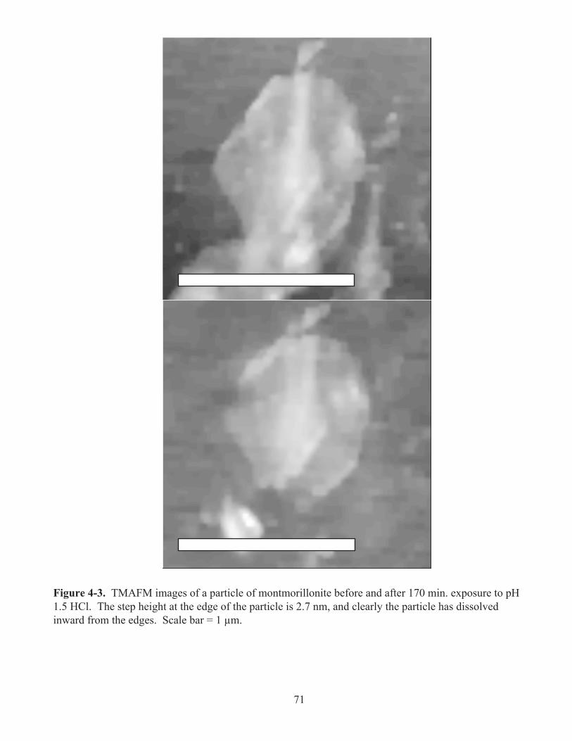
Figure 4-3. TMAFM images of a particle of montmorillonite before and after 170 min. exposure to pH 1.5 HCl. The step height at the edge of the particle is 2.7 nm, and clearly the particle has dissolved inward from the edges. Scale bar = 1 µm.
71

y = 0.00011995xR2 = 0.95515698
0
1E-16
2E-16
3E-16
4E-16
5E-16
6E-16
7E-16
8E-16
0 1E-12 2E-12 3E-12 4E-12 5E-12 6E-12
Vol^0.5 (m^1.5)
Ae
(m^2
)
Figure 4-4. Plot of Ae vs. V1/2 for a montmorillonite particle dissolving at pH 1. The regression line is forced through the origin, still producing an excellent fit of the data. This shows that it is reasonable to assume that the shapes of clay particles stay essentially constant as they dissolve inward from the edges. The slope of the line is used as the b parameter in the calculation of Ae-normalized rates using the shrinking plate model. This parameter effectively serves as a mathematical description of the shape of the platy particle.
72

0
2E-20
4E-20
6E-20
8E-20
1E-19
1.2E-19
0 5000 10000 15000 20000
time (s)
mol
es p
rese
nt
Figure 4-5. Plot of the number of moles present in a montmorillonite particle (the same particle discussed in Fig. 4-4) dissolving in pH 1.0 HCl over time. The diamonds are data points collected from AFM images, and the curved line represents the predicted evolution of the particle, using the shrinking plate model.
73

0
1E-08
2E-08
3E-08
4E-08
5E-08
6E-08
7E-08
8E-08
9E-08
0.5 1 1.5 2 2.5
pH
Biotite MontmorilloniteHectorite Phlogopite
Rat
e (m
ol/m
^2•s
)
Figure 4-6. Ae-normalized dissolution rates for several 2:1 phyllosilicates in the pH range of interest (pH 1-2). Data for biotite and montmorillonite were taken from this study, except the biotite dissolution rate at pH 1.08, which was recalculated from the data of Turpault and Trotignon (1994). The hectorite rate was taken from Bosbach et al. (2000), and the phlogopite rate was taken from Rufe and Hochella (1999).
74

-12
-10
-8
-6
-4
0.5 1.0 1.5 2.0 2.5
pH
At-normalized Ae-normalized
Log
Rat
e (m
ol/m
^2•s
)
Figure 4-7. Ae-normalized biotite dissolution rates reported in this study, and BET-normalized (At) rates from Kalinowski and Schweda (1996) and Malmström and Banwart (1997). The Ae-normalized rates are ~75-400x the Ab-normalized rates. This difference can be explained in terms of the proportion of Ae, high energy sites at freshly ground edges, and the formation of leached layers.
75

-14
-12
-10
-8
-6
-4
0.5 1.0 1.5 2.0 2.5
pH
At-normalized Ae-normalized
Log
Rat
e (m
ol/m
^2•s
)
Figure 4-8. Ae-normalized montmorillonite dissolution rates reported in this study, and EGME-normalized (At) rates from Zysset and Schindler (1996). The Ae-normalized rates are ~26,000-28,000x the At-normalized rates. This difference cannot be explained in terms of the proportion of Ae, high energy sites at freshly ground edges, and the formation of leached layers, but can be explained if it is taken into account that the samples dissolved by Zysset and Schindler were likely flocculated in the reactor.
76

Barry R. Bickmore Chapter 5: Edge Structure and Dissolution Mechanism
77
Chapter 5: Hectorite and NontroniteDissolution: Implications For Phyllosilicate
Edge Structures and Dissolution Mechanisms
Introduction
Atomic Force Microscopy (AFM) has proven to be a powerful tool to explore various
aspects of the structure, microtopography, and surface reactivity of minerals (see Nagy and
Blum, 1994; Hochella, 1995; Hochella et al., 1998). Perhaps its greatest strength, from a
geochemical perspective, has been the ability to make quantitative measurements of changing
surface microtopography in situ, as minerals react in aqueous solutions (Drake et al., 1989;
Hillner et al., 1992; Dove and Hochella, 1993; Bosbach and Rammensee, 1994; Dove and
Chermak, 1994; Junta and Hochella, 1994; Bosbach et al., 1995; Putnis et al., 1995; Bosbach and
Hochella, 1996; Bosbach et al., 1996; Grantham and Dove, 1996; Liang et al., 1996; Junta-Rosso
et al., 1997; Bosbach et al., 1998; Teng et al., 1998; Rufe and Hochella, 1999). Such observations
often bring to light the fact that some mineral faces are more reactive than others, and given a
model of the crystallographic structure of these faces, one can sometimes infer the dominant
mechanism(s) of the surface reaction in question (e.g. Liang et al., 1996; Bosbach et al., 1998;
Rufe and Hochella, 1999).
Due to the extreme anisotropy of their structures, phyllosilicate surfaces have been
shown to exhibit strong differential reactivity (Schofield and Samson, 1953; White and Zelazny,
1988; Anderson and Sposito, 1991; Zachara and McKinley, 1993; Bleam, 1993; Turpault and
Trotignon, 1994; Brady et al., 1996). However, until recently the applicability of in situ AFM
techniques to phyllosilicate surface reactivity has been limited due to two major factors. First,
phyllosilicates are generally characterized by only one cleavage plane – perfect cleavage along the
(001) basal surface. While other faces often occur as preferred growth surfaces, in the case of
macroscopic phyllosilicate crystals (e.g. micas) these are usually too narrow or rough for AFM
analysis. Zones of mechanical weakness within micas run parallel to the preferred growth faces
Barry R. Bickmore Chapter 5: Edge Structure and Dissolution Mechanism
78
(Bloss et al., 1959; Klein and Hurlbut, 1993), but the small-scale step features generated by
cleaving these minerals are generally not euhedral, and hence the “edge” faces available for
examination by AFM are randomly-oriented surfaces. This makes possible the comparison of
the reactivity of non-specific edge surfaces with that of the basal planes, but since the structures
of the randomly-oriented surfaces are not strictly crystallographically constrained, specific
mechanistic information is more difficult to infer. Rufe and Hochella (1999) recently overcame
this problem to some extent by pre-etching phlogopite surfaces with HF, in order to examine the
dissolution behavior of etch pits in HCl and deionized H2O with in situ AFM. The etch pits
were essentially euhedral along the preferred growth faces, and similar features have been
generated on various mica surfaces by etching with either HF or fused alkalis (Pandya and
Pandya, 1959; Patel and Ramanathan, 1962). Second, although clay minerals (phyllosilicates
with a Stokes settling diameter of <2 µm) often exhibit euhedral growth faces at their edges, small
enough to examine with AFM, it has been difficult to immobilize such tiny particles on a suitable
substrate for in situ analysis (Dove and Chermak, 1994). However, Bickmore et al. (1999a)
recently described methods for the immobilization of clay minerals for in situ AFM analysis
under various solution conditions, and Bosbach et al. (1999) have applied one of these techniques
to examine the dissolution behavior of single crystallites of hectorite clay in HCl.
In this paper, we compare the results of Bosbach et al. (1999) on hectorite dissolution
with the in situ AFM nontronite dissolution results of this study. We relate the observed
differential reactivity of the crystal faces to models of the atomic structure of phyllosilicate edge
faces, and determine which one best explains our data. Within the framework of the chosen
model of the edge surface structure, we then relate our results to current models of the proton-
promoted dissolution of phyllosilicates, and determine which one best accounts for the data
obtained in this and other studies.
The structure and reactivity of phyllosilicate surfaces is of fundamental importance for
the understanding of ion mobility in the near-surface environment, permeability reduction in
reservoir rocks, and many other geochemical processes (e.g. Sposito, 1984; Eslinger and Pevear,
1988). In situ AFM imaging of reactions on phyllosilicate surfaces presents the possibility of

Barry R. Bickmore Chapter 5: Edge Structure and Dissolution Mechanism
79
acquiring information about these topics that would, at best, be very difficult to obtain via other
experimental methods now available.
Materials and Methods
Samples
Hectorite.
A sample of hectorite (SHCa-1, Hector, California) was obtained from the Clay Minerals
Society Source Clay Repository. Hectorite Na0.80(Mg5.30Li0.70)(Si7.90Al0.10)O20(OH)4 (Schlegel et
al., 1999) is a trioctahedral, magnesian smectite with some Li substituting for Mg in the
octahedral layer. The <2 µm fraction of the sample material was collected, sodium saturated, acid
washed, and treated with dithionate-citrate-bicarbonate and H2O2 solutions. A more complete
description of the preparation and characterization procedures can be found in Schlegel et al.
(1999).
The hectorite crystallites are predominantly lath-shaped, the long edges representing
(010) surfaces, and the short edge surfaces representing (110), (110), (100), or broken edges
(Oberlin and Méring, 1966; Güven, 1988; Bosbach et al., 1999).
Nontronite
We obtained the nontronite sample from Ward’s (nontronite #33A, Garfield,
Washington). Garfield nontronite Na0.96(Fe3+3.96Mg0.02Ti0.02)(Si6.94Al1.06)O20(OH)4 (Bonnin et al.,
1985) is a dioctahedral smectite with the montmorillonite structure (Eggleton, 1977; Besson et al.,
1982; Besson et al., 1983; Bonnin et al., 1985; Manceau et al., 1998). The sample was crushed in
a mortar and pestle, suspended in 500 ml of deionized H2O, and blended in a Waring heavy-duty
blender for several minutes. Large fragments were allowed to settle out of the suspension, and
the supernatant was decanted. The < 2 µm fraction of the suspension was separated by
centrifugation. In order to remove associated Fe oxides (predominantly goethite, see Güven,
1991; Murad, 1987), the < 2 µm fraction was carefully subjected to several sedimentation cycles
in deionized H2O (Manceau et al., 1998). The sample was then acid washed 4 times by shaking
for one hour in pH 3.0 HCl, and centrifuging. It was then Na-saturated. Approximately 280 mg

Barry R. Bickmore Chapter 5: Edge Structure and Dissolution Mechanism
80
of the purified sample was mounted on a ceramic tile for powder X-ray Diffraction analysis
(Rich, 1969), and no secondary phases were detected.
The Garfield nontronite crystallites are predominantly lath-shaped (Güven, 1991), the
long edges representing (010) faces (Grim and Güven, 1978; Güven, 1991), and the short edges
representing (110), (110) (White and Zelazny, 1988), (100), or broken edge faces.
Clay immobilization
The clays were immobilized for in situ AFM analysis using variations on one of the
techniques described by Bickmore et al. (1999a). The exact procedure used for the hectorite
sample is described by Bosbach et al. (1999). With the nontronite sample, polyethyleneimine
(C2H5N)n (M.W. 1800, Polysciences, Warrington, Pennsylvania) was diluted 1:500 by volume.
A small disc of freshly-cleaved muscovite was taped with double-sided tape to a similarly-
shaped steel AFM sample puck and immersed in the suspension for ~30 s. The muscovite was
then rinsed with a stream of deionized water for 5 min and dried in a 90°C oven for 20 min. A
dilute suspension of the clay in deionized H2O (~0.2 mg clay per 20 ml) was prepared and then
dispersed for 1-2 min. with an Artek sonic dismembrator (Dynatech Laboratories, Chantilly,
Virginia, model 300) set at ~150 Watts. The dried PEI-coated muscovite was immersed in the
clay suspension for 1 min, and then blown dry with a stream of compressed air.
AFM imaging
Imaging of both the hectorite and nontronite crystallites was performed in the fluid cell of
a MultiMode atomic force microscope (Digital Instruments, Santa Barbara, California). Hectorite
imaging was performed with pyramidal Si3N4 tips, while nontronite imaging was performed with
oxide-sharpened Si3N4 tips. Bosbach et al. (1999) reported that force–distance curves showed a
large attractive peak due to the presence of the PEI coating, whereas on clean mica surfaces in
aqueous solution there were not such strong adhesive interactions with the AFM tip. This
sometimes made it difficult to collect stable images in TappingMode (TMAFM), so contact
mode was exclusively used to observe the hectorite dissolution reactions. The strong attraction
between the AFM tip and the PEI-coated mica substrate resulted in a tip loading force of about
50 – 100 nN, and therefore some hectorite particles were stripped from the surface during the

Barry R. Bickmore Chapter 5: Edge Structure and Dissolution Mechanism
81
course of the experiments. Tip-sample interaction can result in enhanced dissolution rates of
monolayer steps (Park et al., 1996), but Bosbach et al. (1999) reported that they could detect no
relationship between scan speed or AFM feedback control parameters and particle edge
dissolution rates. Similarly, we have performed some nontronite dissolution experiments in
TMAFM, which results in a much weaker tip-sample interaction (Hansma et al., 1994; Johnson,
1995). However, we found that contact-mode imaging did, in fact, enhance the nontronite
dissolution rate in a very specific manner, which will be discussed below.
Bosbach et al. (1999) imaged the hectorite under deionized water, and then pH 2.0 HCl
was injected into the cell, after which dissolution was observed. The same procedure was used
with the nontronite, although pH 1.5-2.0 HCl solutions were used.
The AFM images are constructed from height data, and were subjected to the flattening
routine (a least-squares polynomial fit to remove unwanted features from the scan lines) included
with the Digital Instruments software. 5-10 repetitions of a 3x3 median filter were also applied
to the images to remove random noise (Russ, 1995). Analysis of features in the images was
accomplished using the ImageSXM image analysis program (Barrett, 1997).
Crystal structure modeling
The crystal structures and surface planes of hectorite and nontronite were modeled using
the CrystalMaker program for the Macintosh (Palmer, 1996; cf. Koretsky et al., 1998). Data
used to generate models of the nontronite structure were taken from Besson et al. (1983) and
Bonnin et al. (1985). The unit cell parameters used to calculate site densities for nontronite are
a=5.28 Å, b=9.14 Å, c=10.1 Å, and β=99°. Atomic coordinates for hectorite were obtained from
Oberlin and Méring (1966), as were the a and b parameters. The β angle was estimated at 99˚, in
agreement with the discussion of smectite minerals in Deer et al. (1992). Given the above, the c
cell parameter was adjusted to produce a d001 spacing of 9.65 Å, as measured for dehydrated Na-
hectorite by Kadi-Hanifi and Méring (1972). Thus, the unit cell parameters chosen for hectorite
are a=5.25 Å, b=9.09 Å, c=9.77 Å, and β=99°.
The site densities on the (010), (110), and (110) faces of hectorite and nontronite were
calculated by counting the number of sites per planar cell for the (hkl) in question. The planar

Barry R. Bickmore Chapter 5: Edge Structure and Dissolution Mechanism
82
cell areas were calculated by taking the cross product of the vectors defining the parallelogram
which outlines a planar cell on that face (Boisen and Gibbs, 1985). Given the above, the unit cell
face areas for nontronite are A(010) = 0.527 nm2, and A(110) = A( 110 ) = 1.063 nm2, and the unit cell
face areas for hectorite are A(010) = 0.507 nm2, and A(110) = A( 110 ) = 1.080 nm2.
Results and Discussion
Differential reactivity of crystal faces
Hectorite dissolution
Bosbach et al. (1999) report that the dissolution of the hectorite laths appeared to occur
exclusively at the edge surfaces during the time scale of the experiments (up to several hours). A
continuous decrease in particle volume occurred. The particle length/width ratio did not change
significantly during the dissolution process, which, given the morphology of the crystallites,
suggested that the average dissolution rate at the ends of the laths (usually broken edges) was
about 6 times faster than at the lath sides, which were generally euhedral (010) faces. Even
euhedral edges of the laths appeared to “roughen” slightly over time (see Fig. 1). The basal (001)
surfaces did not appear to participate in the reaction.
Nontronite dissolution
The nontronite also appeared to dissolve exclusively from the edges during the time scal
of these experiments (up to 5 hours). Particle heights for several flat laths were measured over
time during contact mode dissolution experiments using smoothed height histograms of the area
of the image around each particle (Bickmore et al., 1999b), and it was found that the particle
height did not significantly change over time. For instance, height measurements over time for
several very flat nontronite laths, observed in various dissolution experiments, are plotted in Fig.
2. Significant dissolution of all these particles was observed at the edges, but the particle heights
did not change appreciably over time except for the two tallest particles in the plot, off of which
approximately 5 Å of detrital material was immediately cleared, and then no further height change
was observed. Similarly, no etch pits were observed to form on the basal surfaces of the laths.
The average measured particle heights for the laths analyzed for Fig. 2 generally were 3.3-3.5 nm,

Barry R. Bickmore Chapter 5: Edge Structure and Dissolution Mechanism
83
and one was ~1.7 nm. These values are consistent with 2 or 1 unit cell high particles,
respectively, since the height of one T-O-T layer (0.9-1 nm) plus the height of a monolayer of
PEI (0.6 ±0.3 nm) (Bickmore et al., 1999a; Bosbach et al., 1999) would be approximately 1.2-1-9
nm, and the added height of another T-O-T layer plus a Na-saturated interlayer (0.5-1 nm) (**)
would result in a particle height of 2.7-3.9 nm.
Very little dissolution even at the edge surfaces of the nontronite laths was observed in
TMAFM, except where ragged edges seemed to straighten somewhat so that the edges more
exactly paralleled the euhedral edge faces.
In contact mode, however, the dissolution at the edges was enhanced in two ways. First,
due to the large tip-sample attraction, long, thin portions of the laths were sometimes broken off
by the AFM tip, creating a high-energy, randomly oriented surface. Second, the tip sometimes
appeared to “nick” the edges of the particles, again creating a high-energy, randomly oriented
defect surface. Both the broken edges and the defect sites dissolved very quickly, until the
dissolution front became pinned parallel to the (010), (110), and (110) edges. In rare cases, (100)
growth surfaces were observed, which sometimes appeared to be stable under acid conditions.
However, the reaction fronts at broken edges and defect sites were never observed to stabilize
along the (100) plane. This behavior is clearly illustrated in Fig. 3, which is a time series of AFM
images taken during the dissolution of several nontronite crystallites in pH 2.0 HCl. The
dissolution behavior of the two laths near the center of the images is especially relevant. Fig. 3a
was taken under deionized water, while Fig. 3b was taken just 6 min. after injection of the acid.
At 6 min. exposure, the outline of the laths appear to have “sharpened” along the (010), (110),
and (110) faces. At 38 min. exposure (Fig. 3c), the probe tip appears to have nicked the top lath
at point A, and the dissolution front has retreated to the point where it has started to approximate
the euhedral face angles. Similarly, the tip appears to have nicked the bottom lath at point B, and
the dissolution front there has proceeded inward and then been pinned along the euhedral face
planes. After 60 min. exposure (Fig. 3d), the outline of the top lath appears to have remained
fairly stable, whereas the probe tip appears to have broken off the end of the bottom lath at point

Barry R. Bickmore Chapter 5: Edge Structure and Dissolution Mechanism
84
C, and nicked it at point D, after which the dissolution fronts in these areas proceeded inward
until they again became pinned parallel to the directions of the euhedral faces.
Edge vs. basal reactivity
As noted above, the basal surfaces of neither the hectorite nor the nontronite particles
appeared to significantly participate in the dissolution reactions within the time scale of these
experiments (up to several hours). This is to be expected, since the basal surfaces are
characterized exclusively by charge-satisfied and extremely stable siloxane bonds, whereas the
edge surfaces are characterized by broken bonds and a well-known tendency to form inner-sphere
complexes with protons and other cations (e.g. White and Zelazny, 1988; Zachara and
McKinley, 1993; Charlet et al., 1993; Schlegel et al., 1999). Similarly, Turpault and Trotignon
(1994) dissolved macroscopic flakes of biotite of known dimensions in pH 1.08 HNO3 at 24 °C,
and demonstrated that the edge surfaces were approximately 250 times more reactive than the
basal surfaces. In addition, Rufe and Hochella (1999) performed in situ TMAFM acid
dissolution experiments on pre-etched phlogopite surfaces, and found that the dissolution
reaction in its early stages occurs via retreat of monolayer edge steps while basal surfaces remain
stable. Based on 19F MAS NMR data, Kaviratna and Pinnavaia (1994) inferred that the acid
hydrolysis of fluorohectorite proceeded almost exclusively at the edge surfaces, and only in its
late stages at the basal surfaces. Since our experiments lasted no more than several hours, our
data are consistent with these studies, and also with the general consensus over several decades
that the acid hydrolysis of 2:1 phyllosilicates essentially proceeds exclusively at the edge
surfaces through most of the reaction (see Nagy, 1995, and references therein).
Hectorite vs. nontronite edge reactivity
The difference in reactivity between the hectorite and nontronite edge faces is very
interesting. Whereas the nontronite edges appeared to straighten, to more closely parallel the
euhedral face planes, the hectorite edges roughened over time. Whereas the nontronite edges
dissolved much faster at broken edges and defect sites (whether tip-induced or not), and the
reaction fronts eventually became pinned at the euhedral face plane angles, the hectorite edges all
appeared to dissolve at relatively similar rates.

Barry R. Bickmore Chapter 5: Edge Structure and Dissolution Mechanism
85
Given these observations, we can draw two important conclusions. First, the active sites
at the hectorite edges are all similar in their reactivity. While broken edges may have some
especially reactive sites, which enhance their step retreat rate somewhat, the reactivity of the
euhedral edges was comparable. The fact that the euhedral edges appeared to roughen over time
graphically illustrates that their reactivity is similar to non-euhedral faces. Second, for some
reason the active sites at the nontronite euhedral edges are much, much less reactive than those at
broken edges and defects. It was pointed out that the AFM tip appeared to generate defect sites
at the edges, which greatly enhanced their reactivity. On the other hand, such defects were
undoubtedly generated during the experiments on the hectorite laths, but a similar increase in
reactivity was not observed.
Implications for edge surface structure
Models of phyllosilicate edge structures
These conclusions about the reactivity of hectorite and nontronite edges obviously must
be explained in terms of the atomic structure and reactivity of the edge surfaces in question.
However, given the morphology and chemistry of these minerals, it is not presently possible to
directly probe the structure of specific phyllosilicate edge surfaces using techniques like Low
Energy Electron Diffraction or Scanning Tunneling Microscopy (see Hochella, 1990). To date
models of phyllosilicate edge structure have usually been derived using established
crystallochemical principles (see Bleam, 1993).
Several workers have proposed schematic models of the types of sites available at
phyllosilicate edges, in order to explain their observed pH dependent charge (Schofield and
Samson, 1953; Muljadi et al., 1966; van Santen, 1982). However, others have constructed more
detailed and useful models, taking into account differences in the crystal structure parallel to
preferred growth faces. For instance, White and Zelazny (1988) used the crystal growth theory
of Hartman and Perdock (1955a,b,c; Hartman, 1963, 1973, 1978; cf. Paquette and Reeder, 1990,
Fouke and Reeder, 1992) to predict the topology of edge sites on the (110), (110), and (010)
faces of dioctahedral phyllosilicates. They further speculated that a certain amount of bond
relaxation occurred on the (110) and (110) faces, leaving them uncharged at normal pH levels

Barry R. Bickmore Chapter 5: Edge Structure and Dissolution Mechanism
86
(pH 3-9). Bleam et al. (1993) used an identical method to predict the topology of the same edges
on pyrophyllite, as well as the (100) and (130) faces. However, they did not allow for surface
relaxation, but instead used an unrelaxed surface configuration, and optimized the surface OH
bond vectors to obtain the surface Coulomb energy and proton Coulomb energy for these faces.
Koretsky et al. (1998) predicted the site types and densities on prominent crystal faces of
several minerals, including the kaolinite (010) and (110) edges, by slicing the crystal structures
along planes that produced the minimum total strength of bonds severed, calculated using the
method of Altermatt and Brown (1985). While Koretsky et al. (1998) did not provide
illustrations of the inferred edge surface topologies, it appears from the site types they predicted
that they likely chose to terminate these edge faces along the same planes predicted by crystal
growth theory. As with Bleam et al. (1993), they did not allow for surface relaxation.
We have chosen to interpret our results within the framework of the type of model
articulated by White and Zelazny (1988). As will be shown below, allowing for charge
neutralization via surface relaxation at some edge sites provides us with a rationale for the
exceptionally low reactivity of the preferred growth faces on nontronite. Specifically, the O
atoms connecting between the octahedral and tetrahedral sheets (hereafter designated “connecting
oxygens”) on dioctahedral phyllosilicates are predicted to be fully bonded, and hence less reactive
with respect to proton attack. On the other hand, some of the connecting oxygens at kink sites
on broken edges and the connecting oxygens on trioctahedral edge faces are predicted to be
underbonded. In order to show that this is the case, in the following sections Hartman-Perdock
crystal growth theory will be applied to predict the topology of all the relevant edge surfaces.
Hartman-Perdock crystal growth theory
Hartman and Perdock (1955a,b,c) proposed that the typical morphology of crystals could
be explained in terms of bond energies. Crystal growth is approximated as the formation of
strong bonds between growth units of stoichiometric composition (Grim and Güven, 1978), and
growth faces are observed to lie parallel to one or more continuous chains of strong bonds within
the crystal structure, called Periodic Bond Chains (PBCs). It must be possible to divide the
entire crystal structure into PBCs of stoichiometric composition, which have no bonds in

Barry R. Bickmore Chapter 5: Edge Structure and Dissolution Mechanism
87
common, and a PBC must not entirely consist of periods of other PBCs. Planes parallel to two
or more PBCs exhibit a low surface energy configuration, which results in a prominent, flat (F)
face. Faces parallel to one PBC are stepped (S), and are less prominent than F faces. Kinked (K)
faces are parallel to no PBCs, and due to their high surface energy, usually do not occur as growth
surfaces.
The topology of the predicted F and S surfaces may be inferred by assuming that they are
terminated along the edges of the stoichiometric PBCs. However, Grim and Güven (1978)
pointed out that one cannot realistically impose the condition of stoichiometry on such a
complex structure, and instead defined separate PBCs along chains of oxygen-linked tetrahedral
and octahedral cations. For the purpose of defining edge surface topology, in this paper we will
adhere to the condition of stoichiometry with respect to the phyllosilicate T-O-T layers, unless a
particularly high-energy surface is generated. In addition, all edge sites will be terminated with O
atoms or OH groups.
Prediction of edge surface topology
White and Zelazny (1988) began their analysis of dioctahedral edge structure by defining
the minimum stoichiometric units required for crystal growth, according to PBC theory.
(Obviously this is somewhat of an oversimplification of the actual crystal growth process.) For
2:1 dioctahedral phyllosilicates without ordered substitution, this may be represented by two
tetrahedra connected to a single octahedron, neglecting interlayer cations. The tetrahedron
connected to the top of the octahedron is related to the tetrahedron connected to the bottom by a
center of symmetry, so as not to create a dipole (see Fig. 4). Grim and Güven (1978) and
Hartman (1982) showed that the PBCs in phyllosilicates are along the [110], [100] and [110]
directions, so that a flat (001) face is predicted, as well as stepped (110), (010), and (110) edge
growth faces. Consistent with this, atomically flat (001) faces dominate phyllosilicate crystal
habits, and the predicted edges are the “pseudohexagonal” faces normally observed on euhedral
phyllosilicate crystals. The fundamental crystal growth units are linked together in the PBCs
shematically represented by the polyhedral models shown in Fig. 5, and ball and stick models of
the PBCs, viewed parallel to the chain directions are shown in Fig. 6. It can be seen in this figure

Barry R. Bickmore Chapter 5: Edge Structure and Dissolution Mechanism
88
that edge faces terminated on either side of the chains would result in an equivalent topology.
Also, the chains parallel to the (110) and (110) edges are symmetrically equivalent, so only the
(110) is depicted here.
Bleam et al. (1993) suggested that the previous workers had neglected to describe two
important PBCs in the phyllosilicate structure, parallel to the (100) and (130) edges. They
supported this assertion by citing Sun and Baronnet (1989a,b), who reported synthetically
grown phlogopite crystals with (100) and (130) faces. However, a closer analysis of the
phyllosilicate structure shows that the bond chains parallel to (100) and (130) are what Hartman
and Perdock (1955b) called “zigzag chains”, composed entirely of periods of other PBCs. The
simple fact of their occurrence does not a priori indicate the presence of a PBC parallel to these
faces. Indeed, Lazarenko et al. (1979) catalogued the occurrence of 33 distinct faces on
phlogopite crystals grown in carbonatites, so it seems more realistic to designate (100) and (130)
phyllosilicate edges as rarely-occurring K faces. This conclusion also seems consistent with Sun
and Baronnet’s results, where the (100) and (130) forms were important only under low
supersaturation conditions (Sun and Baronnet, 1989a) and where Cr inhibited the growth of these
faces (Sun and Baronnet, 1989b).
The “zigzag” nature of the chains parallel to (100) and (130) can be clearly seen by
examining the polyhedral representations in Figs. 7-8. In Fig. 7, a dioctahedral sheet structure is
viewed perpendicular to the (001) plane, and tetrahedral elements of the bond chains parallel to
(010), (110), (110), and (100) are highlighted. The chain of bonds parallel to (100) is composed
exclusively of elements of the PBCs parallel to (010), (110), and (110). An identical result is
obtained by examining the octahedral elements of these bond chains, and Fig. 8 shows the same to
be true for the chain parallel to (130). Therefore, when interpreting the observed reactivity of the
(100) growth faces on nontronite and hectorite laths, we will consider them as kinked surfaces
composed of elements of the (010), (110), and (110) faces. (For a trioctahedral structure, the
octahedral chains parallel to (100) and (130) would still be composed entirely of elements of
other PBCs, but their edges would be straight. Perhaps this adds to the stability of these faces
for trioctahedral minerals like phlogopite.)

Barry R. Bickmore Chapter 5: Edge Structure and Dissolution Mechanism
89
The application of PBC theory to trioctahedral phyllosilicates is a somewhat more
complex task. In order to maintain stoichiometry, the minimum growth unit for a trioctahedral T-
O-T layer must consist of 4 tetrahedra and three octahedra, including two M2 and one M1 sites
(see Fig. 9). Polyhedral representations of the PBCs formed by linking these chains are shown in
Fig. 10, and ball and stick models of the PBCs, viewed parallel to the chain directions are shown
in Fig. 11. Again, the bond chains parallel to (110) and (110) are symmetrically equivalent, so
only the (110) is depicted. In Fig. 11a, it can be seen that terminating edge faces on either side of
the (110) and (110) chains would result in an equivalent topology of edge sites. On the other
hand, Fig. 11b shows that terminating edges on either side of the (010) chain would result in two
very different edge site topologies. Whereas one side would be equivalent to the (010) edge of a
dioctahedral phyllosilicate, the other would have M1 octahedra protruding from the surface.
However, a tally of the type and number of bonds severed to generate such surfaces reveals that
two more Si-O bonds per unit cell repeat would have to be broken to generate a surface with
protruding M1 octahedra than to generate one without. Therefore, in our analysis we will
assume that stable (010) surfaces on trioctahedral phyllosilicates have an edge site topology
equivalent to that of a (010) face on a dioctahedral phyllosilicate.
Surface relaxation and observed reactivity
The assumption that surface sites with unsaturated valency are more reactive than fully
saturated sites, using various methods for calculating bond valence, has commonly been used to
explain the differential reactivity of crystal faces (e.g. van Santen, 1982; Ziolkowski, 1986;
Bleam, 1993; Bargar et al., 1997; Towle et al., 1999a,b), with at least qualitative success. We will
make the same assumption here to rationalize the observed reactivity of the nontronite and
hectorite edge faces. Simple Pauling bond strengths will be used, where: ζ = ∑ Z
vi
ii
. In this
equation, ζ is the total bond strength coordinating each O or OH surface site, Zi is the valence of
each cation coordinating the site, and vi is the coordination number of each cation.
Table 1 lists all the sites available on the surfaces of edge faces of nontronite and
hectorite, terminated by the PBCs discussed above. Since we are making generalizations about

Barry R. Bickmore Chapter 5: Edge Structure and Dissolution Mechanism
90
the reactivity of distinct crystal faces, we have ignored the effects of isomorphous substitutions
(see White and Zelazny, 1988). Thus, ideal structures with only one type of tetrahedral cation
(Si4+) and one type of octahedral cation (Fe3+ or Mg2+) are included. In the first column of Table
1 is listed the type of site (O or OH), and the coordinating atoms are listed in the second. The
third column lists the total strength of bonds coordinating each site based on simple Pauling bond
strengths. The fourth column lists the number of each site per unit cell repeat, and the fifth
column lists the same site densities in sites/nm2, using the unit cell face areas calculated above.
In the nontronite structure, the 2-coordinated connecting oxygens on the (110) and (110)
edges are situated adjacent to 1-coordinated oxygens bonded to octahedral Fe. White and
Zelazny (1988) suggested that if the 1-coordinated O were doubly protonated, this Fe-O bond
might lengthen out to a bond strength of near 0, resulting in an uncharged bound water site.
Simultaneously, the bonds to the adjacent 2-coordinated connecting O would shorten, raising the
total bond strength reaching this site to 2, leaving the 2-coordinated oxygen fully charge-satisfied.
Given that at pH values between approximately 3 and 9 the silanol groups at these edges would
be singly protonated, leaving these sites fully charge-satisfied, these faces would normally be
uncharged. However, even at extreme pH levels, the connecting O sites would remain uncharged,
and thus would have a very low affinity for adsorbing protons. On the nontronite (010) faces, all
surface sites are fully bonded, except for adjacent 1-coordinated OH’s bonded to octahedral
cations. Each of these is underbonded by 1/2, and when doubly protonated, they would be
overbonded by 1/2. Again, however, the connecting O sites are fully bonded, and would have a
very low affinity for adsorbing protons.
White and Zelazny (1988) justified their speculations about the surface relaxation
discussed above by citing similar phenomena known to occur at the edges of sepiolite and
palygorskite (Preisinger, 1959), and by the ability of their model to successfully predict observed
anomalies in structural formulae calculated for fine-grained clay minerals. In addition, Childs et
al. (1999) recently observed the presence of five-coordinate Al in allophane using nuclear
magnetic resonance spectroscopy, and suggested these might originate at the edges of incomplete
octahedral layers. Since the proposed bond shifts on dioctahdral clay edges would effectively
Barry R. Bickmore Chapter 5: Edge Structure and Dissolution Mechanism
91
result in five-coordinate octahedral cations, such observations may be significant to White and
Zelazny’s case. In the case of nontronite, even in the bulk the octahedral sheet is severely
distorted, with Fe-O bond lengths ranging from 1.815 Å to 2.062 Å, corresponding to
empirically-determined bond strengths of 0.86 to 0.44 (Altermatt and Brown, 1985). This
suggests that the proposed bond shifts would not be out of the question. Beyond these simple
arguments, molecular modeling calculations are needed to theoretically justify the predicted
surface relaxation.
On the other hand, cutting our crystal models along noneuhedral planes to simulate
broken edges yielded numerous kink sites, often including underbonded connecting oxygens
coordinated to an octahedral cation surrounded by at least two other underbonded anion sites. In
such cases we would not expect a complete neutralization of the surface charge.
Similarly, on both the (010), (110), and (110) edges of hectorite, the underbonded
connecting oxygens are bonded to octahedral cations which are also bonded to another
undersaturated O. The total strength of bonds (Pauling) coordinating each of these oxygens is 1
2/3, so shifting a 1/3 charge from one site to the other would still leave one of the sites
underbonded. Therefore, we would not expect complete autocompensation of the surface charge
on these faces, either.
If it is assumed that the slowest step in the dissolution process of nontronite and
hectorite is the breaking of connecting oxygen bonds between the octahedral and tetrahedral
sheets, the observed differential reactivity is readily explained. That is, all the faces which
dissolve relatively quickly, including all the hectorite edge surfaces and nontronite broken edges,
are predicted to have coordinatively unsaturated connecting oxygens, which would have a high
affinity for attacking protons. On the other hand, the faces observed to dissolve much more
slowly, including nontronite (010), (110), and (110), are predicted to have fully charge-satisfied
connecting oxygens with a much lower affinity for protonation. Even the stability of the (100)
growth faces on the nontronite laths can be explained if we interpret them as K surfaces
composed of elements of the (010), (110), and (110) edges. Thus, it seems to follow that (100)

Barry R. Bickmore Chapter 5: Edge Structure and Dissolution Mechanism
92
growth surfaces would exhibit low reactivity, but established dissolution fronts at broken edges
or defects likely would not show a tendency to become pinned at a K face.
Implications for the mechanism of proton attack
The conclusion that the dissolution rate is controlled by the breaking of bonds to
connecting oxygens between the tetrahedral and octahedral sheets seems inconsistent with the
model of kaolinite dissolution proposed by Wieland and Stumm (1992). In their study, Wieland
and Stumm measured the surface protonation of kaolinite via potentiometric titration, as well as
the dissolution rate, in acidic and basic solutions. They interpreted their results within the
framework of the coordinative chemical model of mineral dissolution developed by Furrer and
Stumm (1986) and Wieland et al. (1988), where dissolution rates of simple oxides in acidic
solutions were shown to be proportional to integral orders of the concentration of protonated
surface species. It was assumed that these integral orders corresponded to the stoichiometry of a
precursor to the rate-controlling activated complex for the dissolution reaction. In the case of
kaolinite, Wieland and Stumm (1992) found that the dissolution rate of the edge surfaces in acid
solution could be modeled as a first-order function of the concentration of protonated aluminol
sites on the edge faces of the mineral. They concluded that the activated complex controlling the
dissolution reaction at the kaolinite edge surface had a stoichiometry of 1 H to 1 Al. Such a
model seems to implicitly assume that all protonated surface groups associated with the
octahedral cations are equally reactive. However, Wieland and Stumm (1992) realized that
“precursor configurations” associated with different surface functional groups might have very
different surface energies, but appealed to Monte-Carlo simulations which showed that the
surface of a dissolving mineral will tend toward a configuration with only one type of surface
complex (Wehrli, 1989). On the other hand, Wieland and Stumm’s (1992) explanation is still
inconsistent with ours, because if the rate-determining step is associated with the hydrolysis of
connecting O bonds, rather than easily-protonated, monodentate aluminol groups, there should be
no such direct link between total surface protonation on aluminol groups and the rate-determining
activated complex.

Barry R. Bickmore Chapter 5: Edge Structure and Dissolution Mechanism
93
In the case of nontronite dissolution, one cannot explain the tendency for the reaction
front to become pinned at the pseudo-hexagonal face angles in terms of a minimization of
protonated surface functional groups associated with the octahedral cations. Such an explanation
might suffice for the (110) and (110) edges, which likely have no such readily-protonated surface
functional groups, but not for the (010) edges, which have a reasonably high density of
amphoteric, monodentate groups coordinated to an octahedral cation. While the density of these
sites on the (010) edges is almost certainly lower than on most broken edges, the difference
cannot be so great as to explain the much, much slower dissolution of the nontronite (010) faces.
Another problem with the model proposed by Wieland and Stumm (1992) is that ab initio
calculations performed by Xiao and Lasaga (1994) predicted the key step in the dissolution of Si-
O-Al groups would be proton adsorption on the connecting oxygens. Also, an adsorbed proton
on one Si-O-Al group was not predicted to significantly affect the dissolution reaction on
neighboring groups. Therefore, the protonation of amphoteric, monodentate surface functional
groups on such surfaces should not control their dissolution rates.
Our explanation of the in situ observations of nontronite and hectorite dissolution is also
consistent with the model of proton attack at the edges of kaolinite proposed by Ganor et al.
(1995). They found that, within experimental error, kaolinite dissolution rates in acid solutions
were first order with respect to the total surface protonation. A model of kaolinite dissolution
was proposed, where the rate-controlling step is the sequential breaking of bonds to connecting
oxygens. They explained the linear dependence of the rates on total surface proton concentration
by assuming equilibrium between the various types of surface protonated sites. Assuming the
activity coefficients and concentrations of the surface species are reasonably constant during the
dissolution reaction, this results in a first-order reaction with respect to total surface proton
concentration. In a similar study, Zysset and Schindler (1996) showed that the proton-promoted
dissolution of montmorillonite is first order with respect to total surface proton concentration,
including protons inferred to have exchanged into the interlayer spaces of the mineral. They
proposed that the dissolution rate is controlled by hydrolysis of either Si-O-Al or Al-OH-Al
bonds, and that protons adsorbed anywhere on the montmorillonite surface can quickly diffuse to
Barry R. Bickmore Chapter 5: Edge Structure and Dissolution Mechanism
94
the active sites. This explanation appears to be nearly equivalent, at least qualitatively, to the
one proposed by Ganor et al. (1995). However, the possibility that the breaking of bonds
between octahedral sites controls the dissolution rate can be excluded on the basis of the hectorite
dissolution data reported by Bosbach et al. (1999), who showed that the step retreat rate for
hectorite was much slower than that for brucite (Jordan & Rammensee, 1996).
Concluding Remarks
The in situ observations of the dissolution of nontronite and hectorite laths described here
have graphically revealed the differential reactivity of various crystal faces on these minerals. We
have shown that if Hartman-Perdock crystal growth theory is applied to the prediction of edge
site topology, and the type of surface relaxation proposed by White and Zelazny (1988) occurs
on these surfaces, a ready explanation for the observed reactivity emerges. That is, dissolution
reactions are observed to be much slower on surfaces where the oxygen atoms connecting the
octahedral and tetrahedral sheets are predicted to be coordinatively saturated. This conclusion
also implies that the hydrolysis of these connecting sites controls the dissolution rate.
Aside from any implications about the dominant mechanism of dissolution, such models
of phyllosilicate edge structure could have a profound effect on geochemical calculations based on
assumed edge site densities. This is especially true with respect to dioctahedral minerals with a
dominantly euhedral habit. For example, two-thirds of the edge surface area on a hexagonal
kaolinite crystal might be charge-free at normal pH levels.
Given the environmental and industrial importance of reactions taking place at the edges
of phyllosilicate minerals, we suggest that further attempts should be made to explore their
structure and reactivity. Given the extant data, two available courses of action seem to present
themselves. First, molecular modeling calculations should be applied to phyllosilicate edge
surfaces to see whether the surface relaxation predicted by White and Zelazny (1988) can be
theoretically justified. Second, Monte-Carlo simulations of the dissolution of phyllosilicate
mineral structures, such as those discussed by Lasaga (1995) for kaolinite, should be performed

Barry R. Bickmore Chapter 5: Edge Structure and Dissolution Mechanism
95
to see which combinations of bond strengths, etc., would result in the kind of differential
reactivity observed in this study.
Acknowledgements
We thank Michel Schlegel for preparing the hectorite suspension. BB, MH, and ER are
grateful for the support of the National Science Foundation (EAR-9628023, EAR-9902996, and
the Graduate Student Fellowship program) and the Petroleum Research Fund administered by the
American Chemical Society (ACS-PRF 31598-AC2 and ACS-PRF 34326-AC2). DB and LC are
grateful for financial support by the Deutscher Akademischer Austauschdienst and the French
Ministery of Foreign affairs.
References Cited
Altermatt, D., and Brown, I.D. (1985) Bond-valence parameters obtained from a systematic
analysis of the inorganic crystal structure database. Acta Crystallographica, B41, 244-
247.
Anderson, S.J., and Sposito, G. (1991) Cesium-adsorption method for measuring accessible
structural surface charge. Soil Science Society of America Journal, 55, 1569-1576.
Bargar, J.R., Towle, S.N., Brown, G.E., Jr., and Parks, G.A. (1997) XAFS and bond-valence
determination of the structures and compositions of surface functional groups and Pb(II)
and Co(II) sorption products on single-crystal α-Al2O3. Journal of Colloid and Interface
Science, 185, 473-492.
Barrett, S.D. (1997) Image analysis and the internet. Scientific Data Management, 1, 18-25.
Besson, G., de la Calle, C., Rautureau, M., Tchoubar, C., Tsipurski, S.I., and Drits, V.A. (1982)
X-ray and electron diffraction study of the structure of the Garfield nontronite.
Developments in Sedimentology, 35, 29-40.
Besson, G., Bookin, A.S., Dainyak, L.G., Rautureau, M., Tsipursky, S.I., Tchoubar, C., and
Drits, V.A. (1983) Use of diffraction and Mössbauer methods for the structural and

Barry R. Bickmore Chapter 5: Edge Structure and Dissolution Mechanism
96
crystallochemical characterization of nontronites. Journal of Applied Crystallography,
16, 374-383.
Bickmore, B.R., Hochella, M.F., Jr., Bosbach, D., and Charlet, L. (1999a) Methods for
performing Atomic Force Microscopy imaging of clay minerals in aqueous solutions.
Clays and Clay Minerals, 47, 573-581.
Bickmore, B.R., Rufe, E., Barrett, S.D., and Hochella, M.F., Jr. (1999b) Measuring discrete
feature dimensions in AFM images with Image SXM. Geological Materials Research, 1,
n.5. See http://gmr.minsocam.org
Bleam, W.F. (1993) Atomic theories of phyllosilicates: Quantum chemistry, statistical
mechanics, electrostatic theory, and crystal chemistry. Reviews of Geophysics, 31, 51-
73.
Bleam, W.F., Welhouse, G.J., and Janowiak, M.A. (1993) The surface Coulomb energy and
proton Coulomb potentials of pyrophyllite {010}, {110}, {100}, and {130} edges.
Clays and Clay Minerals, 41, 305-316.
Bloss, F.D., Shekarchi, E., and Shell, H.R. (1959) Hardness of synthetic and natural micas.
American Mineralogist, 44, 33-48.
Boisen, M.B., and Gibbs, G.V. (1985) Mathematical Crystallography, Reviews in Mineralogy
15, 460 pp. The Mineralogical Society of America.
Bonin, D., Calas, G., Suquet, H., and Pezerat, H. (1985) Sites occupancy of Fe3+ in Garfield
nontronite: A spectroscopic study. Physics and Chemistry of Minerals, 12, 55-64.
Bosbach, D., and Rammensee, W. (1994) In situ investigation of growth and dissolution on the
(010) surface of gypsum by Scanning Force Microscopy. Geochimica et Cosmochimica
Acta, 58, 843-849.
Bosbach, D., Jordan, G., and Rammensee, W. (1995) Crystal growth and dissolution kinetics of
gypsum and fluorite: An in situ Scanning Force Microscope study. European Journal of
Mineralogy, 7, 267-278.
Bosbach, D., and Hochella, M.F. Jr. (1996) Gypsum growth in the presence of growth inhibitors:
a scanning force microscopy study. Chemical Geology, 132, 227-236.

Barry R. Bickmore Chapter 5: Edge Structure and Dissolution Mechanism
97
Bosbach, D., Junta-Rosso, J.L., Becker, U., and Hochella, M.F. Jr. (1996) Gypsum growth in the
presence of background electrolytes studied by Scanning Force Microscopy. Geochimica
et Cosmochimica Acta, 60, 3295-3304.
Bosbach, D., Hall, C., and Putnis, A.. (1998) Mineral precipitation and dissolution in aqueous
solution: in-situ microscopic observations on barite (001) with atomic force microscopy.
Chemical Geology, 151, 143-160.
Bosbach D, Charlet L, Bickmore BR, Hochella, MF, Jr. (1999) The dissolution of hectorite: In-
situ, real-time observations using Atomic Force Microscopy. American Mineralogist, in
press.
Brady, P.V., Cygan, R.T., and Nagy, K.L. (1996) Molecular controls on kaolinite surface
charge. Journal of Colloid and Interface Science, 183, 356-364.
Casey, W.H., Carr, M.J., and Graham, R.A. (1988) Crystal defects and the dissolution kinetics
of rutile. Geochimica et Cosmochimica Acta, 52, 1545-1556.
Charlet, L., Schindler, P.W., Spadini, L., Furrer, G., Zysset, M. (1993) Cation adsorption on
oxides and clays—the Aluminum case. Aquatic Sciences, 55, 291-303.
Childs, C.W., Hayashi, S., Newman, R.H. (1999) Five-coordinate aluminum in allophane. Clays
and Clay Minerals, 47, 64-69.
Deer, W.A., Howie, R.A., and Zussman, J. (1992) An Introduction to the Rock-Forming
Minerals, 2nd edition. Longman Scientific & Technical.
Dove, P., and Chermak, J. (1994) Mineral-water interactions: Fluid cell applications of scanning
force microscopy. In Scanning Probe Microscopy of Clay Minerals (ed. K.L. Nagy and
A.E. Blum), pp. 139-169. The Clay Minerals Society.
Dove, P.M., and Hochella, M.F. Jr. (1993) Calcite precipitation mechanisms and inhibition by
orthophosphate: In situ observations by Scanning Force Microscopy. Geochimica et
Cosmochimica Acta, 57, 705-714.
Drake, B., Prater, C.B., Weisenhorn, A.L., Gould, S.A.C., Albrecht, T.R., Quate, C.F., Cannell,
D.S., Hansma, H.G., and Hansma, P.K. (1989) Imaging crystals, polymers, and processes
in water with the atomic force microscope. Science, 243, 1586-1588.

Barry R. Bickmore Chapter 5: Edge Structure and Dissolution Mechanism
98
Eggleton, R.A. (1977) Nontronite: Chemistry and X-ray diffraction. Clay Minerals, 12, 181.
Eslinger E, and Pevear D. (1988) Clay Minerals for Petroleum Geologists and Engineers. Society
of Economic Paleontologists and Mineralogists.
Fouke, B.W., and Reeder, R.J. (1992) Surface structural controls on dolomite composition:
Evidence from sectoral zoning. Geochimica et Cosmochimica Acta, 56, 4015-4024.
Furrer, G., and Stumm, W. (1986) The coordination chemistry of weathering: I. Dissolution
kinetics of d-Al2O3 and BeO. Geochimica et Cosmochimica Acta, 50, 1847-1860.
Ganor, J., Mogollón, J.L., and Lasaga, A.C. (1995) The effect of pH on kaolinite dissolution
rates and on activation energy. Geochimica et Cosmochimica Acta, 59, 1037-1052.
Grantham, M.C., and Dove, P.M. (1996) Investigation of bacterial-mineral interactions using
Fluid Tapping Mode Atomic Force Microscopy. Geochimica et Cosmochimica Acta, 60,
2473-2480.
Grim, R.E., and Güven, N. (1978) Bentonites. Geology, Mineralogy, Properties and uses.
Developments in Sedimentology, 24. Elsevier.
Güven, N. (1988) Smectites. In Hydrous phyllosilicates (ed. S.W. Bailey), Reviews in
Mineralogy 19, pp. 497-560. Mineralogical Society of America.
Hansma, P.K., Cleveland, J.P., Radmacher, M., Walters, D.A., Hillner, P.E., Bezanilla, M., Fritz,
M., Vie, D., Hansma, H.G., Prater, C.B., Massie, J., Fukunaga, L., Gurley, J., and Elings,
V. (1994) Tapping mode atomic force microscopy in liquids. Applied Physics Letters,
64, 1738-1740.
Hartman, P. (1963) Structure, growth and morphology of crystals. Zeitschrift für
Krystallographie, 119, 65-78.
Hartman, P. (1973) Structure and morphology. In Crystal Growth: An Introduction (ed. P.
Hartman), pp. 367-402. North Holland Publishing Company.
Hartman, P. (1978) On the validity of the Donnay-Harker Law. Canadian Mineralogist, 16,
387-391.
Hartman, P. (1982) On the growth of dolomite and kaolinite crystals. Neues Jahrbuch für
Mineralogie, Monatshefte 1982, 84-92.

Barry R. Bickmore Chapter 5: Edge Structure and Dissolution Mechanism
99
Hartman, P., and Perdock, W.G. (1955a) On the relations between structure and morphology of
crystals. I. Acta Crystallographica, 8, 49-52.
Hartman, P., and Perdock, W.G. (1955b) On the relations between structure and morphology of
crystals. II. Acta Crystallographica, 8, 521-524.
Hartman, P., and Perdock, W.G. (1955c) On the relations between structure and morphology of
crystals. III. Acta Crystallographica, 8, 525-529.
Hillner, P.E., Gratz, A.J., Manne, S., and Hansma, P.K. (1992) Atomic-Scale imaging of calcite
and dissolution in real time. Geology, 20, 359-362.
Hochella, M.F., Jr. (1990) Atomic structure, microtopography, composition, and reactivity of
mineral surfaces. In Mineral-Water Interface Geochemistry (M.F. Hochella, Jr., and A.F.
White), Reviews in Mineralogy 23, pp. 87-132. The Mineralogical Society of America.
Hochella, M.F. Jr. (1995) Mineral surfaces: Their characterization and their chemical, physical
and reactive nature. In Mineral Surfaces (ed. D.J. Vaughan and R.A.D. Pattrick), pp. 17-
60. Chapman & Hall.
Hochella, M.F., Jr., Rakovan, J., Rosso, K., Bickmore, B., and Rufe, E. (1998) New directions in
mineral surface geochemical research using scanning probe microscopy. In Mineral-Water
Interfacial Reactions: Kinetics and Mechanisms (ed. D.L. Sparks and T.J. Grundl), ACS
Symposium Series Vol. 715, pp. 37-56. American Chemical Society.
Johnson, C.A. (1995) Applications of scanning probe microscopy part 4: AFM imaging in fluids
for the study of colloidal particle adsorption. American Laboratory, 27, 12.
Jordan, G., and Rammensee, W. (1996) Dissolution rates and activation energy for dissolution of
brucite (001): A new method based on the microtopography of crystal surfaces.
Geochimica et Cosmochimica Acta, 60, 5055-5062.
Junta, J.L., and Hochella, M.F. Jr. (1994) Manganese (II) oxidation at mineral surfaces: A
microscopic and spectroscopic study. Geochimica et Cosmochimica Acta, 58, 4985-
4999.

Barry R. Bickmore Chapter 5: Edge Structure and Dissolution Mechanism
100
Junta-Rosso, J.L, Hochella, M.F. Jr., and Rimstidt, J.D. (1997) Linking microscopic and
macroscopic data for heterogeneous reactions illustrated by the oxidation of manganese
(II) at mineral surfaces. Geochimica et Cosmochimica Acta, 61, 149-159.
Kadi-Hanifi, M., and Méring, J. (1972) Précisions sur la structure de l’hectorite. C.R. Acad. Sc.
Paris, Série D, 274, 149-151.
Kaviratna, H., & Pinnavaia, T.J. (1994) Acid hydrolysis of octahedral Mg2+ sites in 2:1 layered
silicates: An assessment of edge attack and gallery access mechanisms. Clays and Clay
Minerals, 42, 717-723.
Klein, C., and Hurlbut, C.S., Jr. (1993) Manual of Mineralogy, 21st ed., 681 pp. John Wiley &
Sons.
Koretsky, C.M., Sverjensky, D.A., Sahai, N. (1998) A model of surface site types on oxide and
silicate minerals based on crystal chemistry: Implications for site types and densities,
multi-site adsorption, surface infrared spectroscopy, and dissolution kinetics. American
Journal of Science, 298, 349-438.
Lasaga, A.C. (1995) Fundamental approaches in describing mineral dissolution and precipitation
rates. In Chemical Weathering Rates of Silicate Minerals (ed. A.F. White and S.L.
Brantley), Reviews in Mineralogy 31, pp. 23-86. Mineralogical Society of America.
Lazarenko, E.K., Krochuk, V.M., and Pavlishin, V.I. (1979) New data on the morphology of
phlogopite crystals and their typomorphic significance. Transactions (Doklady) of the
U.S.S.R. Academy of Sciences: Earth Science Sections, 246, 157-159.
Liang, Y., Baer, D.R., McCoy, J.M., Amonette, J.E., and LaFemina, J.P. (1996) Dissolution
kinetics at the calcite-water interface. Geochimica et Cosmochimica Acta, 60, 4883-4887.
Manceau, A., Chateigner, D., and Gates, W.P. (1998) Polarized EXAFS, distance-valence least-
squares modeling (DVLS), and quantitative texture analysis approaches to the structural
refinement of Garfield nontronite. Physics and Chemistry of Minerals, 25, 347-365.
Muljadi, D., Posner, A.M., and Quirk, J.P. (1966) The mechanism of phosphate adsorption by
kaolinite, gibbsite, and pseudoboehmite. Journal of Soil Science, 17, 212-247.

Barry R. Bickmore Chapter 5: Edge Structure and Dissolution Mechanism
101
Murad, E. (1987) Mössbauer spectra of nontronites: structural implications and
characterization of associated iron oxides. Zeits. Pflanzenernaehr. Bodenk. 150, 279-285.
Nagy, K.L. (1995) Dissolution and precipitation kinetics of sheet silicates. In Chemical
Weathering Rates of Silicate Minerals (ed. A.F. White and S.L. Brantley), Reviews in
Mineralogy 31, pp. 173-233. Mineralogical Society of America.
Nagy, K.L., and Blum, A.E., Eds. (1994) Scanning Probe Microscopy of Clay Minerals, CMS
Workshop Lectures vol. 7, 239 pp. Clay Minerals Society.
Oberlin, P.A., and Méring, J. (1966) Observations sur l’hectorite (etude en microscopie et
diffraction electroniques). Bull. Soc. fran. Miner. Crist., LXXXIX, 29-40
Pandya, N.S., and Pandya, J.R. (1959) Etching of mica by fused alkalies. Bulletin of the
National Institute of Sciences of India, 14, 148-151.
Paquette, J., and Reeder, R.J. (1990) New type of compositional zoning in calcite: Insights into
crystal-growth mechanisms. Geology, 18, 1244-1247.
Park, N.-S., Kim, M.-W., Langford, S.C. & Dickinson, J.T. (1996) Atomic layer wear of single-
crystal calcite in aqueous solution using scanning force microscopy. Journal of Applied
Physics, 80, 2680-2686.
Patel, A.R., and Ramanathan, S. (1962) Etching Mica Cleavages. Acta Crystallographica, 15,
860-862.
Preisinger, A. (1959) X-ray study of the structure of sepiolite. In Clays and Clay Minerals,
Proceedings of the 6th National Conference, Berkeley, California, 1957 (ed. A. Swineford),
pp. 61-67. Pergamon Press.
Putnis, A., Junta-Rosso, J.L., and Hochella, M.F. Jr. (1995) Dissolution of barite by a chelating
ligand: An atomic force microscopy study. Geochimica et Cosmochimica Acta, 59,
4623-4632.
Rakovan, J., Becker, U., and Hochella, M.F., Jr. (1999) Aspects of goethite surface
microtopography, structure, chemistry, and reactivity. American Mineralogist, 84, 884-
894.

Barry R. Bickmore Chapter 5: Edge Structure and Dissolution Mechanism
102
Rich, C.I. (1969) Suction apparatus for mounting clay specimens on ceramic tile for x-ray
diffraction. Soil Science Society of America Proceedings, 33, 815-816.
Rufe, E., and Hochella, M.F., Jr. (1999) Quantitative assessment of reactive surface area of
phlogopite dissolution during acid dissolution. Science, 285, 874-876.
Russ, J.C. (1995) The Image Processing Handbook, 2nd Ed., 674 pp. CRC.
Schlegel, M.L., Manceau, A., Chateigner, D., and Charlet, L. (1999) Sorption of metal ions on
clay minerals: I. Polarized EXAFS evidence for the adsorption of Co on the edges of
hectorite particles. Journal of Colloid and Interface Science, 215, 140-158.
Schofield, R.D., and Samson, H.R. (1953) The deflocculation of kaolinite suspensions and the
accompanying change over from positive to negative chloride adsorption. Clay Minerals
Bulletin, 2, 45-51.
Sposito, G. (1984) The Surface Chemistry of Soils, 277 pp. Oxford University Press.
Sun, B.N., and Baronnet, A. (1989a) Hydrothermal growth of OH-phlogopite single crystals. I.
Undoped growth medium. Journal of Crystal Growth, 96, 265-276.
Sun, B.N., and Baronnet, A. (1989b) Hydrothermal growth of OH-phlogopite single crystals.
II. Role of Cr and Ti adsorption on crystal growth rates. Chemical Geology, 78, 301-
314.
Teng, H.H., Dove, P.M., Orme, C.A., and De Yoreo, J.J.. (1998) Thermodynamics of Calcite
Growth: Baseline for Understanding Biomineral Formation. Science, 282, 724-727.
Towle, S.N., Brown, G.E., Jr., and Parks, G.A. (1999a) Sorption of Co(II) on metal oxide
surfaces: I. Identification of specific binding sites of Co(II) on (110) and (001) surfaces of
TiO2 (rutile) by Grazing-Incidence XAFS Spectroscopy. Journal of Colloid and Interface
Science, 217, 299-311.
Towle, S.N., Bargar, J.R., Brown, G.E., Jr., and Parks, G.A. (1999b) Sorption of Co(II) on
metal oxide surfaces: II. Identification of Co(II)(aq) adsorption sites on the (0001) and
(1-102) surfaces of α-Al2O3 by Grazing-Incidence XAFS Spectroscopy. Journal of
Colloid and Interface Science, 217, 312-321.

Barry R. Bickmore Chapter 5: Edge Structure and Dissolution Mechanism
103
Turpault M.-P. Trotignon L. (1994) The dissolution of biotite single crystals in dilute HNO3 at
24°C: Evidence of an anisotropic corrosion process of micas in acidic solutions.
Geochimica et Cosmochimica Acta, 58, 2761-2775.
van Santen, R.A. (1982) Chemical-bonding aspects of heterogeneous catalysis. II. Solid acids.
Recueil, Journal of the Royal Netherlands Chemical Society, 101, 157-163.
Wehrli, B. (1989) Monte-Carlo simulations of surface morphologies during mineral dissolution.
Journal of Colloid and Interface Science, 132, 230-242.
White, G.N., and Zelazny, L.W. (1988) Analysis and implications of the edge structure of
dioctahedral phyllosilicates. Clays and Clay Minerals, 36, 141-146.
Wieland, E., Wehrli, B., and Stumm, W. (1988) The coordination chemistry of weathering. III.
A generalization on the dissolution rates of minerals. Geochimica et Cosmochimica Acta,
52, 1969-1981.
Wieland, E., and Stumm, W. (1992) Dissolution kinetics of kaolinite in acidic aqueous solutions
at 25 ºC. Geochimica et Cosmochimica Acta, 56, 3339-3355.
Xiao, Y., and Lasaga, A.C. (1994) Ab initio quantum mechanical studies of the kinetics and
mechanisms of silicate dissolution: H+ (H3O+) catalysis. Geochimica et Cosmochimica
Acta, 58, 5379-5400.
Zachara, J.M., and McKinley, J.P. (1993) Influence of hydrolysis on the sorption of metal
cations by smectites: Importance of edge coordination reactions. Aquatic Sciences, 55,
250-261.
Ziolkowski, J. (1986) Crystallochemical model of active sites on oxide catalysts. Journal of
Catalysis, 100, 45-58.
Zysset, M., and Schindler, P.W. (1996) The proton promoted dissolution kinetics of K-
montmorillonite. Geochimica et Cosmochimica Acta, 60, 921-931.

Barry R. Bickmore Chapter 5: Edge Structure and Dissolution Mechanism
104
Table 1. Site Types and Densities on Nontronite and Hectorite Edge Faces
site type coordinating
atoms
coordinating
bond strength
sites per unit cell
face
Sites per nm2
Nontronite (110) and (110 )
O Si 1 4 3.76O 2 Si 2 8 7.53O Si, 2 Fe 2 2 1.88O Si, Fe 1 1/2† 2 1.88O Fe 1/2‡ 2 1.88
OH 2 Fe 1 2 1.88
Nontronite (010)
O Si 1 2 3.80O 2 Si 2 4 7.59O Si, 2 Fe 2 2 3.80
OH Fe 1/2 2 3.80
Hectorite (110) and (110 )
O Si 1 4 3.70O 2 Si 2 8 7.41O Si, 2 Mg 1 2/3 2 1.85O Mg 1/3 2 1.85
OH 2 Mg 2/3 2 1.85OH Mg 1/3 2 1.85
Hectorite (010)
O Si 1 2 3.94O 2 Si 2 4 7.89O Si, 2 Mg 1 2/3 2 3.94
OH Mg 1/3 2 3.94†These bonds are predicted to shorten, so that the coordinating bond strenth will total 2.
‡These bonds are predicted to lengthen to bond strength 0, so that when the site is doubly
Table 5-1. Site types and densities of nontronite and hectorite edge faces.
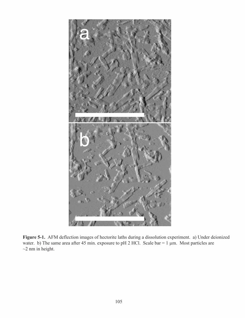
a
b
Figure 5-1. AFM deflection images of hectorite laths during a dissolution experiment. a) Under deionized water. b) The same area after 45 min. exposure to pH 2 HCl. Scale bar = 1 µm. Most particles are ~2 nm in height.
105

Particle Height vs. Time
0
0.5
1
1.5
2
2.5
3
3.5
4
4.5
0 10 20 30 40 50 60 70
time (min)
Figure 5-2. Measured particle heights of several very flat nontronite laths over time during dissolution experiments. While significant dissolution took place at the edges of all these particles, the particle heights appeared to stay essentially constant.
106

a b
c d
B
A
CD
Figure 5-3. AFM height images of nontronite laths after a) 0 min., b) 6 min., c) 38 min., and d) 60 min. of exposure to pH 2 HCl. Scale bar = 1 µm. The two particles in the middle are both ~4 nm in height.
107

Figure 5-4. One stoichiometric crystal growth unit for a dioctahedral 2:1 phyllosilicate, assuming random substitutions.
108

(a) (b)
Figure 5-5. Stoichiometric Periodic Bond Chains (PBCs) for a dioctahedral 2:1 phyllosilicate. a) Chain running parallel to the (110) face. The ( ) face is symmetrically equivalent. b) Chain running parallel to the (010) face.
109

Si Fe O OH
(a) (b)
110
Figure 5-6. Ball and stick models of the Periodic Bond Chains (PBCs) in Fig. 5, viewed parallel to the PBC vector. a) Chain parallel to the (110) face. The ( ) face would be symmetrically equivalent. b) Chain parallel to the (010) face.

(110)PBC
(110)PBC(010)
PBC
(010)PBC
(110)PBC
(110)PBC
(100)Chain
(100)Chain
_
_
Figure 5-7. Polyhedral representation of a dioctahedral T-O-T layer. The highlighted tetrahedra are part of the bond chains indicated in the figure. It can clearly be seen that the chain parallel to the (100) face is composed entirely of elements of the (110), ( ), and (010) Periodic Bond Chains (PBCs). Thus, (100) should not be treated as a PBC.
111

(010)PBC
(010)PBC
(110)PBC
(110)PBC
(130)Chain
(130)Chain
(110)PBC
_
(110)PBC
_
Figure 5-8. Polyhedral representation of a dioctahedral T-O-T layer. The highlighted tetrahedra are part of the bond chains indicated in the figure. It can clearly be seen that the chain parallel to the (130) face is composed entirely of elements of the (110), ( ), and (010) Periodic Bond Chains (PBCs). Thus, (130) should not be treated as a PBC.
112

Figure 5-9. One stoichiometric crystal growth unit for a trioctahedral 2:1 phyllosilicate, assuming random substitutions.
113

(a) (b)Figure 5-10. Stoichiometric Periodic Bond Chains (PBCs) for a trioctahedral 21 phyllosilicate. a) Chain running parallel to the (110) face. The ( ) face is symmetrically equivalent. b) Chain running parallel to the (010) face.
114

Si Fe O OH
(a) (b)
Figure 5-11. Ball and stick models of the Periodic Bond Chains (PBCs) in Fig. 10, viewed parallel to the PBC vector. a) Chain parallel to the (110) face. The ( ) face would be symmetrically equivalent. b) Chain parallel to the (010) face.
115

Barry R. Bickmore Vita
116
Vita
“I Am Barry” or “Nobody is Going to Read This, Anyway”I am Barry, hear me snore
because I’m so smart I am boredAnd I know too much to go back an' pretend
'cause I've heard it all beforeAnd I've been down there on the floor
No one's ever gonna keep me down again
CHORUS:
Oh yes I am wiseBut it's wisdom born of pain
Yes, I've paid the priceBut look how much I gained
If I have to, I can do anything

Barry R. Bickmore Vita
117
I am strong (strong)I am invincible (invincible)
I am Barry
You can bend but never break me'cause it only serves to make me
More determined to achieve my final goalAnd I come back even stronger
Not a novice any longer'cause you've deepened the conviction in my soul
CHORUS:
I am Barry watch me blowthe competition out the do’
As I spread my heap big mojo across the landBut I'm still an embryo
With a long long way to goUntil I make my future bosses understand
Oh yes I am wiseBut it's wisdom born of pain
Yes, I've paid the priceBut look how much I gained
If I have to I can face anythingI am strong (strong)
I am invincible (invincible)I am Barry
Oh, I am BarryI am invincible
I am strong
FADEI am Barry
I am invincibleI am strongI am Barry