Embed Size (px)
Citation preview
ATTACHMENT 4
Instrument Setpoint Calculation Methodology
---
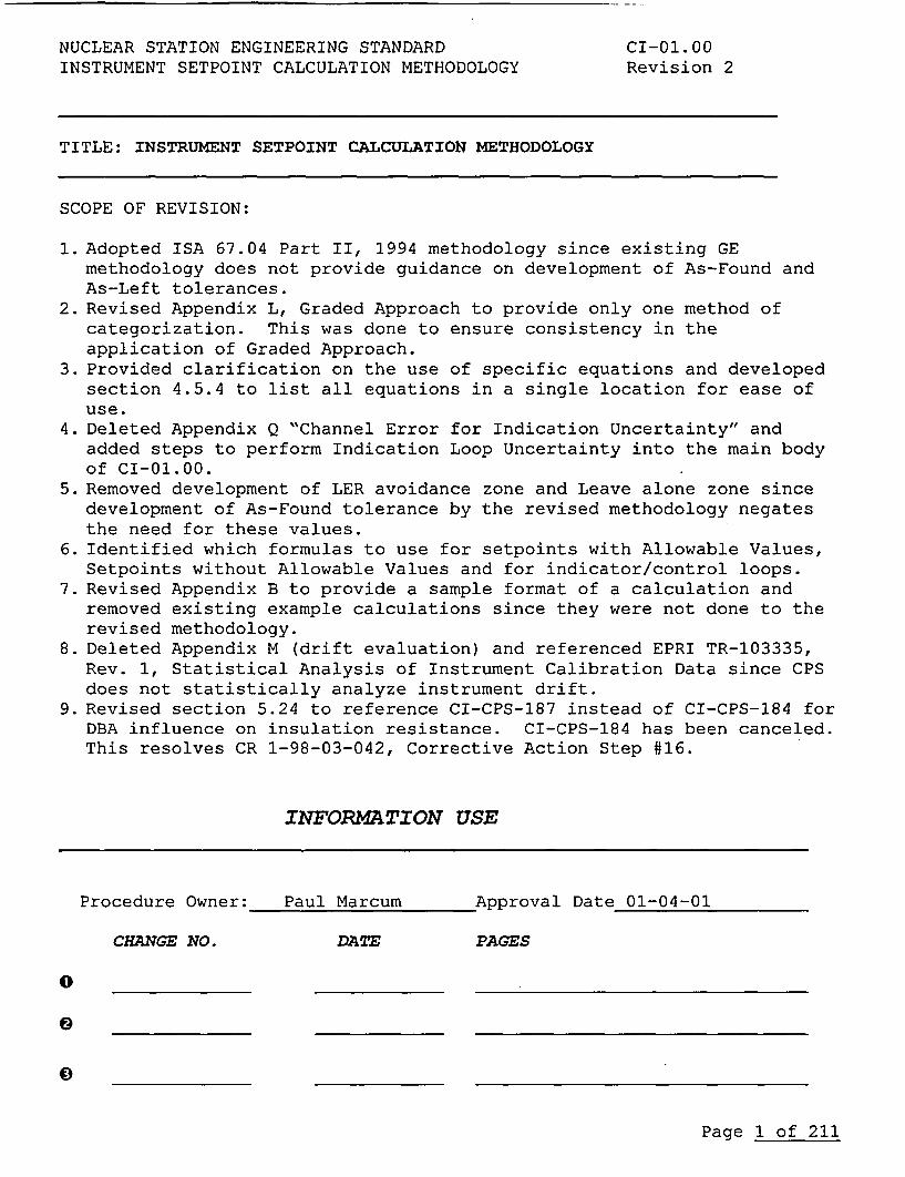
NUCLEAR STATION ENGINEERING STANDARD CI-01.00INSTRUMENT SETPOINT CALCULATION METHODOLOGY Revision 2
TITLE: INSTRUMENT SETPOINT CALCULATION METHODOLOGY
SCOPE OF REVISION:
1. Adopted ISA 67.04 Part II, 1994 methodology since existing GEmethodology does not provide guidance on development of As-Found andAs-Left tolerances.
2. Revised Appendix L, Graded Approach to provide only one method ofcategorization. This was done to ensure consistency in theapplication of Graded Approach.
3. Provided clarification on the use of specific equations and developedsection 4.5.4 to list all equations in a single location for ease ofuse.
4. Deleted Appendix Q "Channel Error for Indication Uncertainty" andadded steps to perform Indication Loop Uncertainty into the main bodyof CI-01.00.
5. Removed development of LER avoidance zone and Leave alone zone sincedevelopment of As-Found tolerance by the revised methodology negatesthe need for these values.
6. Identified which formulas to use for setpoints with Allowable Values,Setpoints without Allowable Values and for indicator/control loops.
7. Revised Appendix B to provide a sample format of a calculation andremoved existing example calculations since they were not done to therevised methodology.
8. Deleted Appendix M (drift evaluation) and referenced EPRI TR-103335,Rev. 1, Statistical Analysis of Instrument Calibration Data since CPSdoes not statistically analyze instrument drift.
9. Revised section 5.24 to reference CI-CPS-187 instead of CI-CPS-184 forDBA influence on insulation resistance. CI-CPS-184 has been canceled.This resolves CR 1-98-03-042, Corrective Action Step #16.
INFORMATION USE
Procedure Owner: Paul Marcum Approval Date 01-04-01
CHANGE NO. DATE PAGES
0
Page 1 of 211
NUCLEAR STATION ENGINEERING STANDARDINSTRUMENT SETPOINT CALCULATION METHODOLOGY
CI-01.00Revision 2
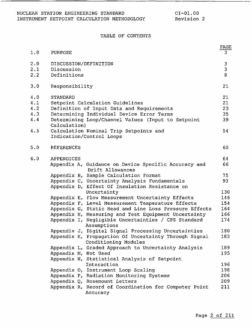
TABLE OF CONTENTS
PAGE31.0
2.02.12.2
PURPOSE
DISCUSSION/DEFINITIONDiscussionDefinitions
338
3.0 Responsibility
4.0 STANDARD4.1 Setpoint Calculation Guidelines4.2 Definition of Input Data and Requirements4.3 Determining Individual Device Error Terms4.4 Determining Loop/Channel Values (Input to Setpoint
Calculation)4.5 Calculation Nominal Trip Setpoints and
Indication/Control Loops
5.0 REFERENCES
21
2121233539
54
60
6.0 APPENDICESAppendix A,
Appendix B,Appendix C,Appendix D,
Appendix E,Appendix F,Appendix G,Appendix H,Appendix I,
Appendix J,Appendix K,
Appendix L,Appendix M,Appendix N,
Appendix 0,Appendix P,Appendix Q,Appendix R,
Guidance on Device Specific Accuracy andDrift AllowancesSample Calculation FormatUncertainty Analysis FundamentalsEffect Of Insulation Resistance onUncertaintyFlow Measurement Uncertainty EffectsLevel Measurement Temperature EffectsStatic Head and Line Loss Pressure EffectsMeasuring and Test Equipment UncertaintyNegligible Uncertainties / CPS StandardAssumptionsDigital Signal Processing UncertaintiesPropagation Of Uncertainty Through SignalConditioning ModulesGraded Approach to Uncertainty AnalysisNot UsedStatistical Analysis of SetpointInteractionInstrument Loop ScalingRadiation Monitoring SystemsRosemount LettersRecord of Coordination for Computer PointAccuracy
6466
7593
130146154164166174
180183
189195
196198206209211
Page 2 of 211
NUCLEAR STATION ENGINEERING STANDARD CI-01.00INSTRUMENT SETPOINT CALCULATION METHODOLOGY Revision 2
1.0 PURPOSE
1.1 The purpose of this Engineering Standard is to provide amethodology for the determination of instrument loopuncertainties and setpoints for the Clinton Power Station.The methodology described in this standard applies touncertainty calculations for setpoint, control, andindication applications.
1.2 This document provides guidelines for the calculation ofinstrumentation setpoints, control, and indicationapplications for the Clinton Power Station.
1.3 These guidelines are applicable to all instrumentsetpoints. They include guidance for calculation of bothAllowable Values and Nominal Trip Setpoints for setpointsincluded in plant Technical Specifications and calculationof Nominal Trip Setpoints for instruments not covered inthe plant Technical Specifications. This document alsoincludes guidance for determination of all input dataapplicable to the calculations as well as important topicsconcerning the interfaces with surveillance and calibrationprocedures and practices.
2.0 DISCUSSION/DEFINITIONS
2.1 Discussion
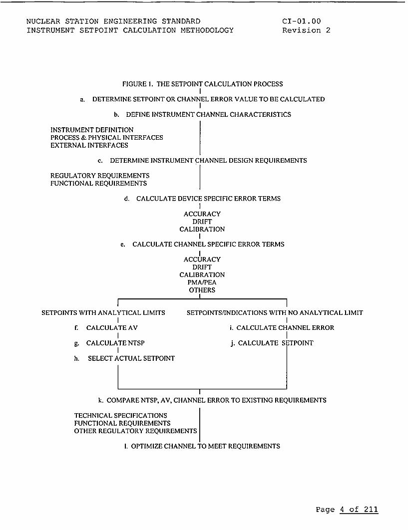
2.1.1 This document is structured to progress through a completecalculation process, from the most detailed level ofindividual device characteristics (drift, accuracy, etc.),through determination of loop characteristics, and finallyto calculation of setpoints and related topics, as outlinedin the following figure:
Definition of Input Data and Requirements
Calculation of Individual Device Terms (device accuracy,drift, etc.)
Combination of Individual Device Terms into Loop Terms(loop accuracy, etc.)
Calculation of Total Channel/Loop Values (Setpoint,Allowable Value, etc.)
Evaluation of Results and Resolution of Problem areas
Supporting Information
Page 3 of 211
NUCLEAR STATION ENGINEERING STANDARDINSTRUMENT SETPOINT CALCULATION METHODOLOGY
CI-01.00Revision 2
FIGURE 1. THE SETPOINT CALCULATION PROCESS
a. DETERMINE SETPOINT OR CHANNEL ERROR VALUE TO BE CALCULATED
b. DEFINE INSTRUMENT CHANNEL CHARACTERISTICS
INSTRUMENT DEFINITIONPROCESS & PHYSICAL INTERFACESEXTERNAL INTERFACES
c. DETERMINE INSTRUMENT CHANNEL DESIGN REQUIREMENTS
REGULATORY REQUIREMENTSFUNCTIONAL REQUIREMENTS
d. CALCULATE DEVICE SPECIFIC ERROR TERMS
ACCURACYDRIFT
CALIBRATION
e. CALCULATE CHANNEL SPECIFIC ERROR TERMS
ACCURACYDRIFT
CALIBRATIONPMA/PEAOTHERS
SETPOINTS WITH ANALYTICAL LIMITS
f. CALCULATE AV
g. CALCULATE NTSP
h. SELECT ACTUAL SETPOINT
SETPOINTS/INDICATIONS WITH NO ANALYTICAL LIMIT
i. CALCULATE CHANNEL ERROR
j. CALCULATE SETPOINT
k. COMPARE NTSP, AV, CHANNEL ERROR TO EXISTING REQUIREMENTS
TECHNICAL SPECIFICATIONSFUNCTIONAL REQUIREMENTSOTHER REGULATORY REQUIREMENTS
1. OPTIMIZE CHANNEL TO MEET REQUIREMENTS
Page 4 of 211
NUCLEAR STATION ENGINEERING STANDARD CI-01.00INSTRUMENT SETPOINT CALCULATION METHODOLOGY Revision 2
2.1.2 Instrument setpoint uncertainty allowances and setpointdiscrepancies are issues that have led to a number ofoperational problems throughout the nuclear industry.Historically CPS instrument loop uncertainty and setpointdetermination had been based upon varying setpointmethodologies. Instrument channel uncertainty andsetpoint determination had been established by twodifferent methods depending on whether or not they appliedto the Reactor Protection System and Engineered SafeguardsFunctions developed by GE or other safety related systems.A third methodology was used to verify that an allowancefor instrument uncertainty was contained in the allowablevalue for Technical Specifications indicating instruments.All three methodologies were rigid in recommendation anddiffered in both process and application. This resultedin CPS instrument uncertainty and setpoint calculationslacking consistent definition of allowable value andimproper understanding of the relationship of theallowable value to earlier setpoint methodologies,procedures, and operability criteria. Beginning with Rev.1, this Engineering Standard is intended to provideconsistency between all CPS instrument setpointcalculations by incorporating the common strengths of eachhistorical methodology into one common method. ThisStandard provides a mechanism for the uniform developmentof new and revised CPS instrument setpoint calculations.This Standard incorporates the common strengths of eachhistorical methodology into one common method consistentwith accepted industry practice.
2.1.3 This standard provides flexibility, then, in the precisemethod by which a setpoint is determined, allowing forvariations in calculation rigor dependent upon thesignificance of the function of the setpoint or operatordecision point. The intent is to provide a format andsystematic method, in contrast with a prescriptive method,of identifying and combining instrument uncertainties. Assuch, this standard provides guidelines to statisticallycombine uncertainties of components in a measurement andperform comparisons to ensure that there is adequatemargin between the setpoint and a given limit to accountfor measurement error. This descriptive systematic methodprovides a consistent criterion for assessing themagnitude of uncertainties associated with eachuncertainty component, thereby ensuring plant safety.
Page 5 of 211
NUCLEAR STATION ENGINEERING STANDARD CI-01.00INSTRUMENT SETPOINT CALCULATION METHODOLOGY Revision 2
2.1.4 A systematic method of identifying and combininginstrument uncertainties is necessary to ensure thatadequate margin has been provided for safety relatedinstrument channels that perform protective functions andfor instrument channels that are important to safety.Thus ensuring that vital plant protective features areactuated at the appropriate time during transient andaccident conditions. Analytical Limits have beenestablished through the process of accident analysis,which assumed that plant protective features wouldintervene to limit the magnitude of a transient. LimitingSafety System Settings (LSSS) are established inaccordance with 10 CFR 50.36. Ensuring that theseprotective features actuate as they were assumed in theaccident analysis provides assurance that safety limitswill not be exceeded. The methodology presented by thisrevision is based on the industry standard ANSI/ISAS67.04, "Setpoints for Nuclear Safety RelatedInstrumentation" Parts I and II(Ref. 5.3), which isendorsed by Regulatory Guide 1.105 (Ref. 5.11). ClintonPower Station (CPS) has invoked RG 1.105 for a basis formeeting the requirements of 10CFR50, Appendix A, generaldesign criterion 13 and 20.
2.1.5 Relation to ISA Standards and Regulatory Guides
2.1.5.1 The applicable ISA Standard for setpoint calculations isISA S67.04. That standard was prepared by a committee ofthe ISA, which included some representatives who alsoparticipated in preparation of the CPS SetpointMethodology. The CPS Setpoint Methodology is consistentwith ISA Standard S67.04.
2.1.5.2 There are three Regulatory Guides related to setpointmethodology; RG 1.105 (Ref. 5.11), RG 1.89 (Ref. 5.35) andRG 1.97 (Ref. 5.34). RG 1.105 covers setpoint methodology.This Setpoint Methodology complies with RG 1.105. RG 1.89covers equipment qualification. This Setpoint Methodologydoes not directly address equipment qualification, beyondthe basic assumption that instrumentation is qualified forits intended service. This Setpoint Methodology may beused to determine instrument errors under variousconditions as part of the process of demonstrating thatinstruments are qualified to perform specified functions,in accordance with RG 1.89. RG 1.97 covers the topic ofpost accident instrumentation. This Setpoint Methodologyalso does not address RG 1.97. However, as is the casewith RG 1.89, the methods of determining instrumentperformance inherent in this Setpoint Methodology may beused when demonstrating that a particular instrumentchannel satisfies the guidance of RG 1.97.
Page 6 of 211
NUCLEAR STATION ENGINEERING STANDARD CI-01.00INSTRUMENT SETPOINT CALCULATION METHODOLOGY Revision 2
2.1.6 In summary, this standard, based upon ISA-S67.04, providesan acceptable method to calculate instrument loop accuracyand setpoints, and applies to NSED as well as anytechnical staff members involved in the modification ofinstrument loops at CPS. The results of an uncertaintyanalysis might be applied to the following types ofcalculations:* Parameters and setpoints that have Analytical Limits* Evaluation or justification of previously established
setpoints* Parameters setpoints that do not have Analytical
Limits.* Determination of instrument indication uncertainties
2.1.7 Setpoints without Analytical Limits
Many, setpoints are important for reliable powergeneration and equipment protection. Because thesesetpoints may not be derived from a safety limit threadedto an accident analysis, the basis for the setpointcalculation is typically developed from process limitsproviding either equipment protection or maintaininggeneration capacity. As defined in Appendix L, "GradedApproach to Uncertainty Analysis", the criteria in thisEngineering Standard may also be used as a guide forsetpoints that do not have Analytical Limits to improveplant reliability, but the calculation may not be asrigorous.
2.1.8 These guidelines are applicable to all instrumentsetpoints. They include guidance for calculation of bothAllowable Values and Nominal Trip Setpoints for setpointsincluded in plant Technical Specifications, andcalculation of Nominal Trip Setpoints for instruments notcovered in plant Technical Specifications.
2.1.9 Indication Uncertainty (Channel Error)
Uncertainty associated with process parameter indicationis also important for safe and reliable plant operation.Allowing for indication uncertainty supports compliancewith the Technical Specifications and the variousoperating procedures. As defined in Appendix L, themethodology presented in this Engineering Standard isapplicable to determining indication uncertainty.
Page 7 of 211
NUCLEAR STATION ENGINEERING STANDARD CI-01.00INSTRUMENT SETPOINT CALCULATION METHODOLOGY Revision 2
2.1.10 Mechanical Equipment Setpoints
This Engineering Standard was developed specifically forinstrumentation components and loops. This EngineeringStandard does not specifically apply to mechanicalequipment setpoints (i.e. safety and relief valvesetpoints) or protective relay applications. However,guidance presented herein may be useful to predict theperformance of other non-instrumentation-type devices.
2.1.11 Rounding Conventions
Normal rounding conventions (rounding up or down dependingon the last digit in the calculated result) do not applyto error calculations or setpoints. All rounding ofresults should be done in the direction, which isconservative relative to plant safety (upward for errorterms, away from the Analytical Limit for Allowable Valuesand Nominal Trip Setpoints). Additionally, all outputvalues to calibration procedures should be in theprecision required by the calibration procedure.
2.2 Definitions
NOTE
The following definitions are based on the methodology of AEDC-31336 (Ref 5.D. IW'here theterms defined are equiv alent to terms used in ISA Standard S67. 04 (Ref 5.3), the equivalenceis noted
2.2.1 AS-FOUND TOLERANCE (AFTL): the tolerance of the As-Founderror in the instrument loop (AFTL), which requirescalibration to restore the loop within the As-LeftTolerance. An as-found tolerance (AFTj) is also developedfor all devices in channel.
2.2.2 ACCURACY TEMPERATURE EFFECT (ATE): The change in instrumentoutput for a constant input when exposed to differentambient temperatures.
2.2.3 ALLOWABLE VALUE (AV): (Technical Specifications Limit):The limiting value of the sensed process variable at whichthe trip setpoint may be found during instrumentsurveillance. Usually prescribed as a license condition.Equivalent to the term Allowable Value as used in ISAStandard S67.04
Page 8 of 211
NUCLEAR STATION ENGINEERING STANDARD CI-01.00INSTRUMENT SETPOINT CALCULATION METHODOLOGY Revision 2
2.2.4 ANALYTICAL LIMIT (AL): The value of the sensed processvariable established as part of the safety analysis priorto or at the point which a desired action is to beinitiated to prevent the safety process variable fromreaching the associated licensing safety limit. Equivalentto the term Analytical Limit as used in ISA StandardS67.04.
2.2.5 AS-LEFT TOLERANCE (ALT1): This tolerance is the precisionwith which the technician should be able to set the deviceduring surveillance. Additionally, if the As-Found valueis within the (ALTi) then re-calibration is not required.The As-Left Tolerance is determined by the organizationresponsible for defining the surveillance procedures(recommendations are provided in this document). A loop as-left tolerance (ALTL) is also developed for all devices inchannel.
2.2.6 BIAS (B): A systematic or fixed instrument uncertainty,which is predictable for a given set of conditions becauseof the existence of a known direction (positive ornegative). See Appendix C, Section C.1.2, for additionaldiscussion.
2.2.7 BOUNDING VALUE (BV): The extreme value of theconservatively calculated process variable that is to becompared to the licensing safety limit during the transientor accident analysis. This value may be either a maximumor minimum value, depending upon the safety variable.
2.2.8 CALIBRATION TOOL ERROR (Ci): The accuracy of the device(multimeter, etc.) being used to perform the calibration orsurveillance test. Also referred to as M&TE (MTE). Fortypical precision equipment CPS recommends that this errorterm be considered to be a 3 sigma value, provided that thecalibration of these devices is to NIST traceable standardsand minimizes the effects of hysterisis, linearity andrepeatability.
2.2.9 CALIBRATION STANDARD ERROR (CSTD): The error in thecalibration of the calibrating tool. Per CPS standardCI-01.00 assumptions, this value considered negligible tothe overall calibration error term and can be ignored.
Page 9 of 211
NUCLEAR STATION ENGINEERING STANDARD CI-01.00INSTRUMENT SETPOINT CALCULATION METHODOLOGY Revision 2
2.2.10 CHANNEL CALIBRATION ACCURACY (CL): The quality of freedomfrom error to which the nominal trip setpoint of a channelcan be calibrated with respect to the true desiredsetpoint. Considering only the errors introduced by theinaccuracies of the calibrating equipment used as thestandards or references and the allowances for errorsintroduced by the calibration procedures. The accuracy ofthe different devices utilized to calibrate the individualchannel instruments is the degree of conformity of theindicated values or outputs of these standards orreferences to the true, exact, or ideal values. The valuespecified is the requirement for the combined accuracies ofall equipment selected to calibrate the actual monitoringand trip devices of an instrument channel plus allowancesfor inaccuracies of the calibration procedures. Channelcalibration accuracy does not include the combinedaccuracies of the individual channel instruments that areactually used to monitor the process variable and providethe channel trip function.
2.2.11 CHANNEL INSTRUMENT ACCURACY (AL): The quality of freedomfrom error of the complete instrument channel with respectto acceptable standards or references. The value specifiedis the requirement for the combined accuracy's of allcomponents in the channel that are used to monitor theprocess variable and/or provide the trip functions andincludes the combined conformity, linearity, hysteresis andrepeatability errors of all these devices. The accuracy ofeach individual component in the channel is the degree ofconformity of the indicated values of that instrument tothe values of a recognized and acceptable standard orreference device (Usually National Bureau of Standardstraceable), that is used to calibrate the instrument.Channel instrument accuracy, channel calibration accuracy,and channel instrument drifts are considered to beindependent variables. This definition encompasses theterms Vendor Accuracy, Hysteresis, and Repeatabilitydefined in ISA Standard S67.04.
2.2.12 CHANNEL INSTRUMENT DRIFT (DL): The change in the value ofthe process variable at which the trip action will occurbetween the time the nominal trip setpoint is calibratedand a subsequent surveillance test. The initial designdata considers drift to be an independent variable. Asfield data is acquired, it may be substituted for theinitial design information. This term is equivalent to theDrift Uncertainty (DR) term used in the ISA StandardS67.04.
Page 10 of 211
NUCLEAR STATION ENGINEERING STANDARD CI-01.00INSTRUMENT SETPOINT CALCULATION METHODOLOGY Revision 2
2.2.13 CHANNEL INDICATION UNCERTAINTY (CE): This is a predictionof error in an indicator or data supply channel resultingfrom all causes that could reasonably be expected duringthe time the channel is performing its function. This termis not used in setpoint calculations.
2.2.14 CONFIDENCE LEVEL: The relative frequency that thecalculated statistic is correct.
2.2.15 CONFIDENCE INTERVAL: The frequency that an intervalestimate of a parameter may be expected to contain the truevalue. For example, 95% coverage of the true value means,that in a repeated sampling, when 95% uncertainty intervalis constructed for each sample, over the long run, theintervals will contain the true value 95% of the time.
2.2.16 CPS STANDARD CI-01.00 ASSUMPTIONS: Assumptions establishedby the Setpoint Program that are considered to bedefendable and should be used without modification to anynew or revised calculation, performed under thismethodology, as applicable. See Appendix I, Section I.11for the current standard assumptions. However, it shouldbe noted, that specific assumptions germane to theindividual calculation shall follow all standardassumptions.
2.2.17 DEADBAND: The range within which the input signal can varywithout experiencing a change in the output.
2.2.18 DESIGN BASIS EVENT (DBE): The limiting abnormal transientor an accident which is analyzed using the analytical limitvalue for the setpoint to determine the bounding value of aprocess variable.
2.2.19 FULL SPAN/SCALE (FS): The highest value of the measuredvariable that device is adjusted to measure.
2.2.20 HARSH ENVIRONMENT: This term refers to the worstenvironmental conditions to which an instrument is exposedduring normal, transient, accident or post-accidentconditions, out to the point in time when the device is nolonger called upon to serve any monitoring or tripfunction. This term may be used in Equipment Qualificationto define the qualification conditions.
From the standpoint of establishing setpoints, HarshEnvironment does not apply. This distinction is made toavoid confusion between the long-term functionalrequirements for the devices, which includes post-tripoperation, and the operational requirements during theinitial period leading to the first trip.
2.2.21 HUMIDITY EFFECT (HE): Error due to humidity.
Page 11 of 211
NUCLEAR STATION ENGINEERING STANDARD CI-01.00INSTRUMENT SETPOINT CALCULATION METHODOLOGY Revision 2
2.2.22 HYSTERESIS: An instrument's change in response as theprocess input signal increases or decreases (see Fig. C-5).
2.2.23 INDICATOR READING ERROR (IRE): The error applied to theaccuracy with which personnel can read the analog anddigital indications in an instrument loop or on M&TE. Thisvalue will normally be one quarter of the smallest divisionof the scale. IRE is not required IF the device ALT isrounded to the nearest conservative half-minor division.For non-linear scales the IRE may be evaluated for the areaof interest. Appendix C provides in depth discussion andusage guidelines for IRE.
2.2.24 INSTRUMENT CHANNEL: An arrangement of components requiredto generate a protective signal, or, in the case ofmonitoring channels, to deliver the signal to the point atwhich it is monitored. Unless otherwise stated, it isassumed that the channel is the same as the loop.Equivalent to the term Instrument Channel in ISA StandardS67.04.
2.2.25 INSTRUMENT RESPONSE TIME EFFECTS: The delay in theactuation of a trip function following the time when ameasured process variable reaches the actual trip setpointdue to time response characteristics of the instrumentchannel.
2.2.26 INSULATION RESISTANCE ACCURACY ERROR (IRA): This is theerror effect produced by degradation of insulationresistance (IR), for the various cables, terminal boardsand other components in the instrument loop, exclusive ofother defined error terms (Accuracy, Calibration, Drift,Process Measurement Accuracy, Primary Element Accuracy).Since the effect of current leakage associated with IRA ispredictable and will act only in one direction for a givenloop, IRA is always treated as a bias term in calculations.
2.2.27 LICENSEE EVENT REPORT (LER): A report which must be filedwith the NRC by the utility when a technical specificationslimit is known to be exceeded, as required by 10CFR50.73.
2.2.28 LICENSING SAFETY LIMIT (LSL): The limit on a safety processvariable that is established by licensing requirements toprovide conservative protection for the integrity ofphysical barriers that guard against uncontrolled releaseof radioactivity. Events of moderate frequency, infrequentevents, and accidents use appropriately assigned licensingsafety limits. Overpressure events use appropriatelyselected criteria for upset, emergency, or faulted ASMEcategory events. Equivalent to Safety Limit in ISAStandard S67.04.
Page 12 of 211
NUCLEAR STATION ENGINEERING STANDARD CI-01.00INSTRUMENT SETPOINT CALCULATION METHODOLOGY Revision 2
2.2.29 LIMITING SAFETY SYSTEMS SETTING (LSSS): A term used in theTechnical Specifications, and in ISA Standard S67.04, torefer to Reactor Protection System (nominal) trip setpointsand allowable values.
2.2.30 LIMITING NORMAL OPERATING TRANSIENT: The most severetransient event affecting a process variable during normaloperation for which trip initiation is to be avoided.
2.2.31 LINEARITY: The ability of the instrument to provide alinear output in response to a linear input (see Fig. C-6).
2.2.32 MEAN VALUE: The average value of a random sample orpopulation. For n measurements of Xi, where i ranging from1 to n, the mean is given by
u = Z XIln
2.2.33 MEASURED SIGNAL: The electrical, mechanical, pneumatic, orother variable applied to the input of a device.
2.2.34 MEASURED VARIABLE: A quantity, property, or condition thatis measured, e.g., temperature, pressure, flow rate, orspeed.
2.2.35 MEASUREMENT: The present value of a variable such as flowrate, pressure, level, or temperature.
2.2.36 MEASUREMENT AND TEST EQUIPMENT EFFECT (MTE): Theuncertainty attributed to measuring and test equipment thatis used to calibrate the instrument loop components. Alsocalled Calibration Tool Error (Ci).
2.2.37 MILD ENVIRONMENT: An environment that at no time is moresevere than the expected environment during normal plantoperation, including anticipated operational occurrences.
2.2.38 MODELING ACCURACY: The modeling accuracy may consist ofmodeling bias and/or modeling variability. Modeling biasis the result of comparing analysis models used in eventanalysis to actual plant test data or more realisticmodels. Modeling variability is the uncertainty in theability of the model to predict the process or safetyvariable.
2.2.39 MODULE: Any assembly of interconnecting components, whichconstitutes an identifiable device, instrument or piece ofequipment. A module can be removed as a unit and replacedwith a spare. It has definable performance characteristics,which permit it to be tested as a unit. A module can be acard, a drawout circuit breaker or other subassembly of alarger device, provided it meets the requirements of thisdefinition.
Page 13 of 211
NUCLEAR STATION ENGINEERING STANDARD CI-01.00INSTRUMENT SETPOINT CALCULATION METHODOLOGY Revision 2
2.2.40 MODULE UNCERTAINTY (Ai): The total uncertainty attributableto a single module. The uncertainty of an instrument loopthrough a display or actuation device will include theuncertainty of one or more modules.
2.2.41 NOISE: An unwanted component of a signal or variable. Itcauses a fluctuation in a signal that tends to obscure itsinformation content.
2.2.42 NOMINAL TRIP SETPOINT (NTSP): The limiting value of thesensed process variable at which a trip may be set tooperate at the time of calibration. This is equivalent tothe term Trip Setpoint in ISA Standard S67.04.
2.2.43 NOMINAL VALUE: The value assigned for the purpose ofconvenient designation but existing in name only; thestated or specified value as opposed to the actual value.
2.2.44 NONLINEAR: A relationship between two or more variablesthat cannot be described as a straight line. When used todescribe the output of an instrument, it means that theoutput is of a different magnitude than the input, e.g.,square-root relationship.
2.2.45 NORMAL DISTRIBUTION: The density function of the normalrandom variable x, with mean p and variance a2 is:
nl (x;,u a) e 2a'2
2.2.46 NORMAL PROCESS LIMIT (NPL): The safety limit, high or low,beyond which the normal process parameter, should notvary. Trip setpoints associated with non-safety-relatedfunctions might be based on the normal process limit.
2.2.47 NORMAL ENVIRONMENT: The environmental conditions expectedduring normal plant operation.
2.2.48 OPERATIONAL LIMIT (OL): The operational value of a processvariable established to allow trip avoidance margin forthe limiting normal operating transient.
2.2.49 OVERPRESSURE EFFECT (OPE): Error due to overpressuretransients (if any).
2.2.50 POWER SUPPLY EFFECT (PSE): Error due to power supplyfluctuations.
2.2.51PRIMARY ELEMENT ACCURACY (PEA): The accuracy of the device(exclusive of the sensor) which is in contact with theprocess, resulting in some form of interaction (e.g., in anorifice meter, the orifice plate, adjacent parts of the
Page 14 of 211
NUCLEAR STATION ENGINEERING STANDARD CI-01.00INSTRUMENT SETPOINT CALCULATION METHODOLOGY Revision 2
pipe, and the pressure connections constitute the primaryelement).
2.2.52 PROBABILITY: The relative frequency with which an eventoccurs over the long run.
2.2.53 PROCESS MEASUREMENT ACCURACY (PMA): Process variablemeasurement effects (e.g., the effect of changing fluiddensity on level measurement) aside from the primaryelement and the sensor.
2.2.54 RADIATION EFFECT (RE): Error due to radiation.
2.2.55 RANDOM: Describing a variable whose value at a particularfuture instant cannot be predicted exactly, but can onlybe estimated by a probability distribution function. SeeAppendix C, Section C.1.1, for additional discussion.
2.2.56 RANGE: The region between the limits within which aquantity is measured, received, or transmitted, expressedby stating the lower and upper range values.
2.2.57 REPEATABILITY: The ability of an instrument to produceexactly the same result every time it is subjected to thesame conditions (see Figure C-4).
2.2.58 REQUIRED LIMIT (RL): A criterion sometimes applied to As-Found surveillance data for judging whether or not thechannel's Allowable Value could be exceeded in asubsequent surveillance interval.
2.2.59 REVERSE ACTION: An increasing input to an instrumentproducing a decreasing output.
2.2.60 RFI/EMI EFFECT (REE): Error due to RFI/EMI influences (ifany).
2.2.61 RISE TIME: The time it takes a system to reach a certainpercentage of its final value when a step input is applied.Common reference points are 50%, 63%, and 90% rise times.
2.2.62 RPS: Reactor Protection System.
2.2.63 RTD: Resistance Temperature Detector.
2.2.64 SAFETY LIMIT (Licensing Safety Limit): A limit on animportant process variable that is necessary to reasonablyprotect the integrity of physical barriers that guardagainst the uncontrolled release of radioactivity.
Page 15 of 211
NUCLEAR STATION ENGINEERING STANDARD CI-01.00INSTRUMENT SETPOINT CALCULATION METHODOLOGY Revision 2
2.2.65 SAFETY-RELATED INSTRUMENTATION: Instrumentation that isessential to the following:
* Provide emergency reactor shutdown* Provide containment isolation* Provide reactor core cooling* Provide for containment or reactor heat removal* Prevent or mitigate a significant release of
radioactive material to the environment or isotherwise essential to provide reasonable assurancethat a nuclear power plant can be operated withoutundue risk to the health and safety of the public
Other instrumentation, such as certain Regulatory Guide1.97 instrumentation, may be treated as safety relatedeven though it may not meet the strict definition above.
2.2.66 SEISMIC EFFECT (SE): The change in instrument output for aconstant input when exposed to a seismic event of specifiedmagnitude.
2.2.67 SENSOR (TRANSMITTER): The portion of the instrumentchannel, which converts the process parameter value to anelectrical signal. This is equivalent to ISA StandardS67.04.
2.2.68 SIGMA: The value specified is the maximum value of astandard deviation of the probability distribution of theparameter based on a normal distribution.
2.2.69 SIGNAL CONVERTER: A transducer that converts onetransmission signal to another.
2.2.70 SPAN: The algebraic difference between the upper and lowervalues of a range.
2.2.71 SPAN SHIFT: An undesired shift in the calibrated span of aninstrument (see Figure C-8). Span shift is one type ofinstrument drift that can occur.
2.2.72 SQUARE-ROOT EXTRACTOR: A device whose output is the squareroot of its input signal.
Page 16 of 211
NUCLEAR STATION ENGINEERING STANDARD CI-01.00INSTRUMENT SETPOINT CALCULATION METHODOLOGY Revision 2
2.2.73 SQUARE-ROOT-SUM-OF-SQUARES METHOD (SRSS): A method ofcombining uncertainties that are random, normallydistributed, and independent.
2=
2.2.74 STANDARD DEVIATION (POPULATION): A measure of how widelyvalues are dispersed from the population mean and is givenby
_n x2 - )2
n(n -1)
2.2.75 STANDARD DEVIATION (Sample): A measure of how widely valuesare dispersed from the sample mean and is given by
_n x 2 - (ZX)2
n2
2.2.76 STATIC PRESSURE: The steady-state pressure applied to adevice.
2.2.77 STATIC PRESSURE EFFECT (SPE): The change in instrumentoutput, generally applying only to differential pressuremeasurements, for a constant input when measuring adifferential pressure and simultaneously exposed to astatic pressure. May consist of three effects:
(SPEs) Static Pressure Span Effect (random)
(SPEz) Static Pressure Zero Effect (random)(SPEBS) Bias Span Effect (bias)
2.2.78 STEADY-STATE: A characteristic of a condition, such asvalue, rate, periodicity, or amplitude, exhibiting only anegligible change over an arbitrary long period of time.
2.2.79STEADY-STATE OPERATING VALUE (X0): The maximum or minimumvalue of the process variable anticipated during normalsteady-state operation.
2.2.80 SUPPRESSED-ZERO RANGE: A range in which the zero value ofthe measured variable is less than the lower range value.
2.2.81 SURVEILLANCE INTERVAL: The elapsed time between theinitiation or completion of successive surveillance's orsurveillance checks on the same instrument, channel,instrument loop, or other specified system or device.
Page 17 of 211
NUCLEAR STATION ENGINEERING STANDARD CI-01.00INSTRUMENT SETPOINT CALCULATION METHODOLOGY Revision 2
2.2.82 TEST INTERVAL: The elapsed time between the initiation orcompletion of successive tests on the same instrument,channel, instrument loop, or other specified system ordevice.
2.2.83 TIME CONSTANT: For the output of a first-order systemforced by a step or impulse, the time constant T is thetime required to complete 63.2% of the total rise ordecay.
2.2.84 TIME-DEPENDENT DRIFT: The tendency for the magnitude ofinstrument drift to vary with time.
2.2.85 TIME-INDEPENDENT DRIFT: The tendency for the magnitude ofinstrument drift to show no specific trend with time.
2.2.86 TIME RESPONSE: An output expressed as a function of time,resulting from the application of a specified input underspecified operating conditions.
2.2.87 TOLERANCE: The allowable variation from a specified or truevalue.
2.2.88 TOLERANCE INTERVAL: An interval that contains a definedproportion of the population to a given probability.
2.2.89 TOTAL HARMONIC DISTORTION (THD): The distortion present inan AC voltage or current that causes it to deviate from anideal sine wave.
2.2.90 TRANSFER FUNCTION: The ratio of the transformation of theoutput of a system to the input to the system.
2.2.91 TRANSMITTER (SENSOR): A device that measures a physicalparameter such as pressure or temperature and transmits aconditioned signal to a receiving device.
2.2.92 TRANSIENT OVERSHOOT: The difference in magnitude of asensed process variable taken from the point of tripactuation to the point at which the magnitude is at amaximum or minimum.
2.2.93 TRIP ENVIRONMENT: The environment that exists up to andincluding the time when the instrument channel performs itsinitial safety (trip) function during an event.
Page 18 of 211
NUCLEAR STATION ENGINEERING STANDARD CI-01.00INSTRUMENT SETPOINT CALCULATION METHODOLOGY Revision 2
2.2.94 TRIP UNIT: The portion of the instrument channel whichcompares the converted process value of the sensor to thetrip value, and provides the output "trip" signal when thetrip value is reached.
2.2.95 TURNDOWN RATIO: The ratio of maximum span to calibratedspan for an instrument.
2.2.96 UNCERTAINTY: The amount to which an instrument channel'soutput is in doubt (or the allowance made therefore) due topossible errors either random or systematic which have notbeen corrected for. The uncertainty is generally identifiedwithin a probability and confidence level.
2.2.97 UPPER RANGE LIMIT (URL): The maximum upper calibrated spanlimit for the device.
2.2.98 VENDOR ACCURACY (VA): A number or quantity that defines thelimit that errors will not exceed when the device is usedunder reference operating conditions (see Figure C-3). Inthis context, error represents the change or deviation fromthe ideal value.
2.2.99 VENDOR DRIFT (VD): The drift value identified in vendorspecifications or device testing (history) data.
2.2.100 ZERO: The point that represents no variable beingtransmitted (0% of the upper range value).
2.2.101 ZERO ADJUSTMENT: Means provided in an instrument to producea parallel shift of the input-output curve.
2.2.102 ZERO ELEVATION: For an elevated-zero range, the amount themeasured variable zero is above the lower range value.
2.2.103 ZERO SHIFT: An undesired shift in the calibrated zero pointof an instrument (see Figure C-7). Zero shift is one typeof instrument drift that can occur.
2.2.104 ZERO SUPPRESSION: For a suppressed-zero range, the amountthe measured variable zero is below the lower range value.
2.2.105 The following Abbreviations and Acronyms are used:
AFTi = As-Found ToleranceAi = Device AccuracyAL = Analytical LimitAL = Loop/Channel AccuracyALT = As-Left ToleranceATE = Accuracy Temperature EffectAV = Allowable ValueB = Bias Effect
Page 19 of 211

NUCLEAR STATION ENGINEERING STANDARDINSTRUMENT SETPOINT CALCULATION METHODOLOGY
CI-01.00Revision 2
BV = Bounding Value
Page 20 of 211
NUCLEAR STATION ENGINEERING STANDARD CI-01.00INSTRUMENT SETPOINT CALCULATION METHODOLOGY Revision 2
BWR = Boiling Water ReactorCi = Calibration Device ErrorCE = Channel Indication UncertaintyCU = Channel UncertaintyCL = Loop/Channel Calibration Accuracy ErrorCSTD= Calibration Standard ErrorD = Device DriftDBE = Design Bases EventDL = Loop/Channel DriftECCS= Emergency Core Cooling SystemFS = Full Span/Scale Valueg = Acceleration of gravityHE = Humidity EffectIR = Insulation ResistanceIRA = Insulation Resistance Accuracy ErrorIRE = Indicator Reading ErrorISA = Instrument Society of AmericaLER = Licensee Event ReportLOCA= Loss of Coolant AccidentLSL = Licensing Safety LimitLSSS= Limiting Safety Systems SettingN,n = The number of Standard Deviations (sigma values) usedNIST= National Institutes of Science and TechnologyNPL = Nominal Process LimitNTSP= Nominal Trip SetpointOL = Operational LimitOPE = Overpressure EffectPEA = Primary Element AccuracyPMA = Process Measurement AccuracyPSE = Power Supply EffectRE = Radiation EffectREE = RFI/EMI EffectRFI/EMI = Radio Frequency/Electro-Mechanical InterferenceRG = Regulatory GuideRL = Required LimitRPS = Reactor Protection SystemRTD = Resistance Temperature DetectorSE = Seismic EffectSL = Safety LimitSP = SpanSPE = Static Pressure EffectSPEBs= Bias Span EffectSPEs = Random Span EffectSPEz = Random Zero EffectSRSS = Square root of the sum of the squares.T = TemperatureTHD = Total Harmonic DistortionURL = Upper Range LimitUSNRC = United States Nuclear Regulatory CommissionVA = Vendor AccuracyVD = Vendor DriftZ = Measure of Margin in Units of Standard DeviationsZPA = Zero Period Accelerationa = Sigma
Page 21 of 211
NUCLEAR STATION ENGINEERING STANDARD CI-01.00INSTRUMENT SETPOINT CALCULATION METHODOLOGY Revision 2
3.0 RESPONSIBILITY
The Supervisor- C&I Design Engineering is responsible forthe implementation of this Standard.
4.0 STANDARD
4.1 Setpoint Calculation Guidelines
The overall process for evaluating instrumentation isdepicted in Figure 1, and described in the sections ofthis document which follow.
4.1.1 Overview
4.1.1.1 Summary of Setpoint Methodology
The Clinton Power Station (CPS) Setpoint Methodology is astatistically based methodology. It recognizes that mostof the uncertainties that affect instrument performanceare subject to random behavior, and utilizes statistical(probability) estimates of the various uncertainties toachieve conservative, but reasonable, predictions ofinstrument channel uncertainties. The objective of thestatistical approach to setpoint calculations is toachieve a workable compromise between the need to ensureinstrument trips when needed, and the need to avoidspurious trips that may unnecessarily challenge safetysystems or disrupt plant operation.
4.1.2 Fundamental Assumptions
4.1.2.1 Treatment of Uncertainties
The first fundamental assumption of the CPS SetpointMethodology is that all uncertainties related toinstrument channel performance may be treated as acombination of bias and/or independent randomuncertainties. It is assumed that, although all randomuncertainties might not exhibit the characteristics of anormal random distribution, the random terms may beapproximated by a random normal distribution, such thatstatistical methods may be used to combine the individualuncertainties. Thus, a key aspect of properly applyingthis methodology is to examine the various error terms ofinterest and properly classify each term as to whether itrepresents a bias or random term, and then to assignadequately conservative values to the terms.
Page 22 of 211
NUCLEAR STATION ENGINEERING STANDARD CI-01.00INSTRUMENT SETPOINT CALCULATION METHODOLOGY Revision 2
4.1.2.2 Trip Timing
The second fundamental assumption of the CPS SetpointMethodology is that the automatic trip functionsassociated with setpoints are optimized to function intheir first trip during an event, the point in time whenthey (and they alone) are most relied upon for plantsafety. Additional or subsequent trip functions arepermitted to be less accurate because their importance toplant safety (relative to the importance of operatoraction) is less. Worst case environmental conditions,that assume failure of protective equipment, or conditionsthat would only exist after the point in time where manualoperation action is expected are not applicable to theautomatic trip functions that are expected or relied uponto occur in the early part of an event. This assumptionis necessary to ensure that overly conservativeenvironmental assumptions are not permitted to inflateerror estimates, producing overly conservative setpoints,which may themselves lead to spurious trips andunnecessary challenges to safety systems. Paragraph4.2.4.2.(d), discusses determination of trip timing.
4.1.2.3 Instrument QualificationThe third fundamental assumption of the CPS SetpointMethodology is that safety related instrumentation hasbeen qualified to function in the environment expected asa result of plant events. This relates to the secondassumption, above. Specifically, although the setpoint isoptimized for the first trip expected in an event, theinstrumentation might be required to function after thefirst trip. In optimizing the setpoint for the firstautomatic function, it is expected that later automaticfunctions will occur, but with potentially poorer accuracy(see paragraph 4.2.4.2.(d) for further discussion on triptiming). The later automatic functions of theinstrumentation can only be expected if theinstrumentation has been qualified for the expectedenvironmental conditions.
4.1.3.1 Probability Criteria
4.1.3.2 Because the CPS Setpoint Methodology is statisticallybased, it is necessary to establish a desired probabilityfor the various actions associated with the setpoints. Theprobability target is 95%. This value has been accepted bythe USNRC. Appendix C, Uncertainty Analysis Fundamentalsand Reference 5.32, EPRI TR-103335, provide detaildiscussion of the systematic methodology.
Page 23 of 211
NUCLEAR STATION ENGINEERING STANDARD CI-01.00INSTRUMENT SETPOINT CALCULATION METHODOLOGY Revision 2
4.1.3.3 In applying the 95% probability limit, it is important torecognize the form of the data and the objective of thecalculation. For the case of test data or vendor data, the95% probability limit corresponds to plus or minus two (2)standard deviations (i.e., 2 sigma). This represents anormal distribution with 95% of the data in the center, and2.5% each at the upper and lower edges of the distribution.In the case of a setpoint calculation, we are usually notinterested in a plus or minus situation. Instead, sincethe purpose of the trip setpoint is to ensure a trip onlywhen approaching a potentially unsafe condition (onedirection only). CPS is interested in a distribution inwhich 95% is below the trip point, and 5% is beyond thetrip point, all at one end of the normal distribution.This is called a normal one-sided distribution. The pointat which 5% of the cases lie beyond the trip pointcorresponding to 1.645 standard deviations (i.e., 1.645sigma).
4.1.3.4 In performing the setpoint or channel error calculations itwill be important that the probabilities associated withvarious elements of the calculation be known and properlyaccounted for. Scaling and the design requirementsnecessary for implementing process measurement will beevaluated and controlled in a device calculation.
4.1.3.4 In performing the setpoint or channel error calculations itwill be important that the probabilities associated withvarious elements of the calculation be known and properlyaccounted for. Vendor and calibration data will generallybe 2 or 3 sigma values. In determining channel accuraciesand other errors, the data will generally be adjusted to acommon 2 sigma basis. Subsequently in setpointcalculations, etc., the probability limits will be adjustedfrom 2 sigma to the particular probability limit ofinterest.
4.2 Definition of Input Data and RequirementsThis section of this document provides detailed discussionof the input data and requirements that may apply to agiven calculation, in terms of information on thecharacteristics of the instrument channel and theapplicable design requirements. Additional guidance isprovided in Appendix C, and in detailed Appendices, asindicated.
Page 24 of 211
NUCLEAR STATION ENGINEERING STANDARD CI-01.00INSTRUMENT SETPOINT CALCULATION METHODOLOGY Revision 2
4.2.1 Defining Instrument channel characteristics, OverviewThe instrument characteristics to be defined depend on thenature of the instrument channel. Generally, the followinginformation should be included in the instrument channeldesign characteristics:
4.2.1.1 Instrument DefinitionManufacturerModelRangeVendor Performance specificationsTag NumberInstrument Channel Arrangement
4.2.1.2 Process and Physical InterfacesEnvironmental ConditionsSeismic ConditionsProcess Conditions
4.2.1.3 External InterfacesCalibration MethodsCalibration TolerancesInstallation InformationSurveillance IntervalsExternal ContributionsProcess MeasurementPrimary ElementSpecial terms and Biases
Each of these aspects is discussed in more detail in thefollowing Section
4.2.2 Defining Instrument Channel Characteristics
4.2.2.1 Instrument Definition
a. Manufacturer, Model, Tag Number, InstrumentArrangement
The instrument tag number, Manufacturer and modelnumber are determined from controlled designinformation or by examination of the actualinstruments. Instrument channel arrangement refers tothe schematic layout of the channel, including boththe physical layout and the electrical connections.The physical layout is important for devices that maybe exposed to static head or local environmentalconditions, so that the conditions can be properlyaccounted for in the calculations. The electricalconnections are of importance because the actualmanner in which the devices in a channel are connectedaffects the combination of error terms, particularlywith regard to estimating calibration errors.
Page 25 of 211
NUCLEAR STATION ENGINEERING STANDARD CI-01.00INSTRUMENT SETPOINT CALCULATION METHODOLOGY Revision 2
b. Instrument Range
The instrument range for each device in the instrumentchannel includes at least four terms.
The Upper range limit(URL) of the instrument and thecalibrated span (SP) of the device. The last two, arethe range of the input signal to the device, and thecorresponding range of output signal produced inresponse to the input.
As an illustration, consider a typical channelconsisting of a pressure transmitter connected to atrip unit and a signal conditioner leading to anindicator channel:
The maximum pressure range over which the transmitteris capable of operating is the URL. The processpressure range for which the transmitter is calibratedis the SP.
The output signal range of the transmitter is theelectrical output(volts or milliamps) corresponding tothe calibrated span.
The input to the trip unit and the signal conditionerwould be the electrical input corresponding to theelectrical output of the transmitter. In a similarfashion, the input and output ranges for every devicein the instrument channel is defined by establishingthe electrical signal that corresponds to thecalibrated span of the transmitter.
c. Vendor Performance Specifications
Vendor performance specifications are the terms thatidentify how the individual devices in an instrumentchannel are expected to perform, in terms of accuracy,drift, and other errors. All error terms identified inmanufacturers performance data should be consideredfor potential applicability to the calculation oferrors. In addition, the results of plant specific orgeneric Equipment Qualification (EQ) programs shouldbe considered. When EQ program data applicable to aparticular application indicates different performancecharacteristics than that published in open vendordata, the limiting or most conservative data will beused. If additional margin is required, then thedifferences should be resolved. In order to assureconsistency in combining errors in an instrumentchannel, vendor performance specifications must beexpressed as a percentage of Upper Range, CalibratedSpan, or the electrical input or output ranges of thedevices.
Page 26 of 211
NUCLEAR STATION ENGINEERING STANDARD CI-01.00INSTRUMENT SETPOINT CALCULATION METHODOLOGY Revision 2
4.2.2.2 Process and Physical Interfaces
a. Environmental Conditions
Up to four distinct sets of environmental conditionsmust be defined for a given instrument channel.
* The first of these is the set of environmentalconditions that applies at the time the instrumentsare calibrated. Under normal conditions, the onlyenvironmental condition of interest duringcalibration is the possible range of temperatures.This is of interest because temperature changesbetween subsequent calibrations can introduce atemperature error, which becomes part of theapparent drift of the device.
* The second distinct set of environmental conditionsis the plant normal conditions. These are thecombination of radiation, temperature, pressure andhumidity that are expected to be present at themounting locations of each of the devices duringnormal plant operation under conditions where theinstrument is in use. These conditions are used toestimate normal errors, particularly in thespurious trip margin evaluation.
* The third distinct set of environmental conditionsto be identified is the trip environmentalconditions. These are the combination of radiation,temperature, pressure and humidity expected to bepresent at the mounting location of each device atthe point in time that the device is relied upon toperform its automatic trip function. Theseenvironmental conditions are generally those thatmay exist at the first trip of an automatic system,before the operator takes control of an event.
* The fourth distinct set of environmental conditionsthat may be needed is the long-term post-accidentenvironmental conditions. These conditions do notapply to most setpoints, but may apply forevaluations of channel error for post-accidentmonitoring and long-term core cooling (or similar)functions.
Page 27 of 211
NUCLEAR STATION ENGINEERING STANDARD CI-01.00INSTRUMENT SETPOINT CALCULATION METHODOLOGY Revision 2
4.2.2.2 (cont'd)* In all cases, it should be noted that the
environmental conditions of importance are thoseseen by all the devices in the instrument channel.This includes equipment, which connects to theinstrument, such as instrument lines. For example,instrument lines, which pass through multiple areas(particularly the Drywell) will experience statichead variations due to the temperature effects onthe fluid in the lines (see Process MeasurementAccuracy of Appendix C).
b. Seismic Conditions
* Seismic conditions ("g" loads) apply to setpointsassociated with events that may occur during orafter an earthquake. Depending on the type ofinstrument (and the manufacturer's definition ofhow seismic loads affect the devices) two differentseismic conditions may be of interest. These arethe seismic loads that may occur prior to the timethe instrument performs its function, and theseismic loads that may be present while theinstrument is performing its function. In general,the seismic loading of interest is the Zero PeriodAcceleration at the point the instrument ismounted.
c. Process Conditions
As discussed in Appendix C, three sets of processconditions may be of importance for most instrumentchannels.
* The first of these is the calibration conditionsthat may be present at the time the device iscalibrated. This is generally of interest fordevices such as differential pressure transmitters,which are calibrated at zero static pressure, butthen operated when the reactor is at normaloperating pressure. The change in static pressureconditions must be known and accounted for incalibration and/or channel error calculations.
* The second set of process conditions of interest isthe set of worst case conditions that may be imposedon the instrument from within the process. Certaintypes of pressure transmitters, for example, aresubject to overpressure errors if subjected topressures above a specified value.
Page 28 of 211
NUCLEAR STATION ENGINEERING STANDARD CI-01.00INSTRUMENT SETPOINT CALCULATION METHODOLOGY Revision 2
* The third set of process conditions of interest isthe conditions expected to be present when theinstrument is performing its function. Conceivably,this can be more than one set of conditions. Theseprocess conditions determine the errors that mayexist when the instruments are calibrated atdifferent process conditions, and may also affectthe magnitude of Process Measurement Accuracy andPrimary Element Accuracy terms in the setpoint orchannel error calculations.
4.2.2.3 External (outside world) Interfaces
a. Calibration Methods and Tolerances
Calibration methods and tolerances are of importancebecause they have an effect on many aspects of thesetpoint or channel error evaluations. They determinethe channel calibration error, and may also be used todetermine As-Found and As-Left tolerances. Calibrationtolerances can be identified in a number of differentways. If the plant operating personnel have evaluatedtheir calibration procedures and established an overallchannel calibration error for each channel, then thisinformation may be used directly in setpointcalculations. If not the following information shouldbe obtained, so that the channel calibration error canbe determined:
1. A list of the instruments used to calibrate thechannel.
2. A calibration diagram, showing the locations in theinstrument channel where calibration signals areinput or measured, the type and accuracy ofinstruments used at each location, and values ofcalibration signals.
3. If known, accuracy of the NIST or equivalentCalibration standards used to calibrate devicessuch as pressure gauges used in the calibration.
4. If established, As-Left and As-Found tolerancesused in calibration of each of the devices.
b. Installation Information
Installation information of interest includes theinstalled instrument arrangement, including allconnections to the process, instrument line routings,panel and rack locations and elevations, etc.Elevations and instrument line routings are importantfor determining head corrections, Process MeasurementAccuracy and Primary Element Accuracy, and othereffects associated with instrument physicalarrangement.
Page 29 of 211
NUCLEAR STATION ENGINEERING STANDARD CI-01.00INSTRUMENT SETPOINT CALCULATION METHODOLOGY Revision 2
c. Surveillance Intervals
The surveillance interval associated with each devicein the instrument channel should be determined fromthe plant surveillance documents. In general, thesurveillance interval assumed for the setpoint orchannel error calculations should be the longestnormal surveillance interval of any device in thechannel (e.g., 18 months, due to the transmitter). Incases where the calibration interval can be delayed,the maximum interval should be used (e.g., CPSTechnical Specifications allow for calibrationintervals to be delayed for up to 125% of the requiredinterval, or (18 months) * 1.25 = 22.5 months).However, for devices in the instrument channel thatare calibrated on a shorter interval, inaccuraciesneed not be extrapolated to the maximum interval.Refer to Section 4.3.2 for more detail.
d. External Error Contributions
The final step in determining instrument channelcharacteristics is to determine whether the instrumentchannel of interest may be subject to any additionalerror contributions beyond those normally associatedwith the instruments themselves. If any of theseeffects may apply to a particular channel, datanecessary to define the effect must be obtained.Potential External Error Contributions may include:
* Process Measurement Accuracy (PMA)* Primary Element Accuracy (PEA)* Indicator Reading Error (IRE)* Insulation Resistance Accuracy (IRA)* Unique error terms
4.2.3 Instrument Channel Design Requirements
Design requirements applicable to the instrument channelshould be defined, including, as applicable:
4.2.3.1 Regulatory Requirements* Technical Specifications* Safety Analysis Reports* NRC Safety Evaluation Reports* 10CFR50 (particularly Appendix R)
* Regulatory Guides 1.89, 1.97 and 1.105
Page 30 of 211
NUCLEAR STATION ENGINEERING STANDARD CI-01.00INSTRUMENT SETPOINT CALCULATION METHODOLOGY Revision 2
4.2.3.2 Functional Requirements
* Instrument function
* Analytical and Safety Limits
* Operational Limits
* Function Times
* Requirements imposed by plant procedures, EmergencyOperating Procedures (EOPs), etc.
* For indicator or computer channels, allowable channelerror (CE)
Each of these aspects is discussed below.
4.2.4 Defining Instrument Channel Design Requirements
4.2.4.1 Regulatory Requirements
a. Technical Specifications
Technical Specifications requirements are ofimportance for setpoints and instrument channelscovered within the Technical Specifications.Requirements of importance are Surveillance intervals,Allowable Values and Nominal Trip Setpoints specifiedin the Technical Specifications. Existing values inthe Technical Specifications should be reviewed, evenfor new setpoint calculations, because it is usuallydesirable to preserve the existing TechnicalSpecifications values if they can be supported by thesetpoint calculations. Thus, the TechnicalSpecifications values (particularly the AllowableValue and Nominal Trip Setpoint) are used inevaluating the acceptability of calculation results,and may also be used in the evaluation of As-Found andAs-Left Tolerances and determination of RequiredLimits (if used).
b. Safety Analysis Reports, NRC, SERs, 10CFR50,Regulatory Guides
While the Technical Specifications are the keydocuments to examine for regulatory commitments orrequirements, the balance of the plant licensingdocumentation may contain commitments or agreementsreached with the NRC, as well as system specificrequirements that may affect setpoint calculations.Normally, all such commitments or requirements shouldalso be reflected in the applicable plantspecifications and documents. However, the licensingdocumentation should be considered in assuringcommitments are known.
Page 31 of 211
NUCLEAR STATION ENGINEERING STANDARD CI-01.00INSTRUMENT SETPOINT CALCULATION METHODOLOGY Revision 2
4.2.4.2 Functional Requirements
a. Instrument Function
Instrument functional requirements are normallycontained in system Design Specifications, DesignSpecification Data Sheets, Instrument Data Sheets andsimilar documents. The functional requirements to bedetermined should not only include the purpose of thesetpoint, but also the plant operating conditions oroperating modes under which the trip is required to beoperable, and identification of the most severeconditions under which the trip should be avoided.The plant operating conditions under which a trip mustbe operable should be correlated to the licensingbasis events so that the questions of tripenvironment, absence or presence of seismic loads,etc., can be answered.
b. Analytical and Safety Limits
* The Licensing Safety Limit (LSL) is the value of asafety parameter that must not be violated in orderto assure plant safety. In the case of a safetysituation for which there is an accident ortransient analysis, the safety limit is the limitthat the analysis is intended to support. Forsituations where there is no transient analysis,such as the pressure limit for a section of pipe.The Safety Limit or Nominal Process Limit (NPL)would be the limit assumed in design (the Designpressure and Temperature of the pipe, for example).
* The Analytical Limit (AL) is a slightly differentconcept. The Analytical Limit is the value at whichthe trip is assumed to occur, as part of theanalyses, which prove that the Safety Limit issatisfied. For the example of pipe pressure, ifthere is a stress analysis, which assumes that aparticular event is terminated, by instrumentaction, at or before a certain pressure is reached.The pressure at which the instrument is assumed toreact, to terminate the event, is the AnalyticalLimit for that event, even if it is different thanthe Design Pressure of the piping.
* The section of this document dealing with the actualsetpoint calculations gives more specific guidanceon how to select the Analytical Limit to be used.
Page 32 of 211
NUCLEAR STATION ENGINEERING STANDARD CI-01.00INSTRUMENT SETPOINT CALCULATION METHODOLOGY Revision 2
c. Operational Limits (OL)
Operational Limits are the values of the measuredparameter which may occur during plant operation, andat which it would be undesirable to have a trip occur.Usually, there is one limiting Operational Limit for agiven setpoint. In certain cases, such as HighDrywell Pressure, there may be no credible operatingcondition, short of the design basis accident (whichrequires a trip). In such situations, there would beno Operational Limit.
d. Function Times
* Function times should be identified for everyinstrument channel requiring either a setpointcalculation or channel error calculation. Thefunction time is important because it is used todetermine the worst rational environmentalconditions for use in determining instrument error.Caution should be exercised in determining functiontimes. This is because the function time selectedfor a particular case can have a very large impacton instrument error calculations, and this in turncan have a significant impact on the setpoint, andthe risk of spurious trip. That is, over-conservative function times lead to over-conservative setpoints and higher spurious triprisk. Since spurious trips can themselves lead tosafety system challenges, the ultimate result ofover-conservative function times can be a situation,which is counter productive to overall safety.
Page 33 of 211
NUCLEAR STATION ENGINEERING STANDARD CI-01.00INSTRUMENT SETPOINT CALCULATION METHODOLOGY Revision 2
In determining the function time for a particularsetpoint, attention should be given to theconditions under which the operator depends most onthe automatic actions triggered by the setpoint.For example, in the case of a reactor water levelsignal intended to start the ECCS system in theevent of a Loss of Coolant Accident. The operatordepends most on the automatic function during thefirst 10 minutes of the event, before reactor poweris significantly reduced and before the operatorhas had an opportunity to take control of thesituation. During this early period of a LOCA, thecore is not yet uncovered and therefore no coredamage and major radioactive release would beexpected. The operator could reset the water leveltrip devices after the event, but since the reactorwould then be shutdown, and rapidly changing waterlevels would no longer be credible, the need fortrip accuracy would be considerably reduced. Thus,it is appropriate to base the trip setpoint on theconditions existing in the first 10 minutes,without assuming core damage (it should be noted,however, that environmental conditions used forEquipment Qualification might indicate otherwise,since they assume failures).
Note: All setpoints, controls or indications need onlybe evaluated to the worst environmental conditionspresent at the time their function is required.
Page 34 of 211
NUCLEAR STATION ENGINEERING STANDARD CI-01.00INSTRUMENT SETPOINT CALCULATION METHODOLOGY Revision 2
e. Requirements Imposed by Plant Procedures (EOPs, etc.)As defined in Appendix L, plant operating procedures,particularly Emergency Operating Procedures, should beconsidered in defining the functions of instruments.This is particularly important in connection with thetopic of instrument function times, since the PlantProcedures define the extent that the operator maydepend on the instrumentation, and the events forwhich this dependence is most important. Engineeringjudgment must be exercised in evaluating the effect ofoperating procedures. For example, while a particularprocedure may require the operator to reset aparticular trip device, the reset requirement does notnecessarily imply that the instrument must react asaccurately in a subsequent trip. Thus, the firsttrip, prior to the operator taking control, may stillbe the appropriate basis for the setpoint calculation.Engineering judgment and a good understanding of thedesign bases of the plant must be applied toidentifying the impact of Plant Procedures on thefunctional requirements applicable to theinstrumentation.
f. Allowable Channel Error (CE)
As defined in Section 2.2, Channel Error IndicationUncertainty, for certain types of channels,particularly indicator channels and channels whichsupply signals to computers and data collectionsystems, there may be requirements on the maximumallowable error in the channel. Such requirements maybe imposed by the purpose of the indicating functions(such as a Plant procedure requirement), or by the usethat is made of the data. The manner in which theinstrument data is used should be evaluated todetermine if there are any inherent limits onacceptable channel error, independent of the setpointcalculation.
4.2.5 Data Collection
All data collected should be referenced to its source(document number, title, and revision level) and recordedin the Input, Output, or Reference Section of thecalculation, so that the basis for the setpoint or channelerror calculations will be traceable to the proper plantdocuments.
Page 35 of 211
NUCLEAR STATION ENGINEERING STANDARD CI-01.00INSTRUMENT SETPOINT CALCULATION METHODOLOGY Revision 2
4.3 Determining Individual Device Error Terms
4.3.1 Determining Individual Device Accuracies
As defined in Section 2.2, the overall accuracy error forany individual device is developed by combining all theindividual error contributions identified by vendorperformance specifications or device qualification tests.As a means of assuring consideration of all terms, it isuseful to view the accuracy error of the device in terms ofthe factors that might cause the device to exhibit errors.That is, what external or internal effects might affect theperformance of the device? The answer to this question isstraight forward: Device accuracy may be influenced by theinherent precision of the internal components, plus errorscaused by each and every external (environmental) influenceon the device. Specifically, the following potentialcauses of accuracy error should be considered for any givendevice:a. Vendor Accuracy (VA)b. Accuracy Temperature Effect (ATE)c. Overpressure Effect (OPE)d. Static Pressure Effect (SPE)e. Seismic Effect (SE)f. Radiation Effect (RE)g. Humidity Effect (HE)h. Power Supply Effect (PSE)i. RFI/EMI Effect (REE)
The identification of these potential effects is notintended to indicate that they apply to all devices. Firstof all, some suppliers of instrumentation provide a singlevalue of accuracy error, which may already include all ormany of the external environmental effects listed above(within some bounding environment specified by the vendor).Guidance and information for some common devices isprovided in Appendix A and C to this document,additionally, Appendix L, Graded Approach to UncertaintyAnalysis, provides guidance in terms of rigor in whichelements of device uncertainty should be considered duringa calculation.
Following identification of potential effects, each of theerror terms should be examined to determine if it may betreated as a random term, or whether dependencies may existwhich would include systematic or bias error as describedin Appendix C, Sections C.1.1 and C.1.2.
Page 36 of 211
NUCLEAR STATION ENGINEERING STANDARD CI-01.00INSTRUMENT SETPOINT CALCULATION METHODOLOGY Revision 2
Once all the accuracy error contributions for a particularinstrument are identified, they should be combined usingthe SRSS method to determine total device accuracy. Inperforming the SRSS combination, the individual level ofconfidence of each term (sigma level) should be accountedfor such that the resultant device accuracy error is a 2sigma value. Refer to Section C.4 for cases whereinstruments are calibrated together as a rack.
Ai = ± N((VAi/n) 2 + (ATEi/n)2 + (OPEi/n)2 + (SPEi/n)2 +
(SEi/n) 2 + (REi/n) 2 + (HEi/n) 2 + (PSEi/n) 2 + (REEi/n) 2)1 /2
± Any bias term associated with the above randomerrors (2c)
Where the values of 'n' are the sigma values associatedwith each individual effect (i.e., 1, 2, 3) and N is 2 fora 2 sigma value of Ai.
Generally, two accuracy terms are required for setpointcalculations; accuracy under normal plant operatingconditions (AiN) and accuracy under the conditions forwhich the circuit will be required to trip (Al Accident/seismic)-
The Setpoint Program Coordinator can provide samplecalculations.
4.3.2 Determining Individual Device Drift
Drift for individual devices are determined in a mannersimilar to that of accuracy.
Vendor Drift (VD): Refer to Section 2.2 for definition.
The Vendor Drift term should be adjusted to thesurveillance interval for that device. In accordance withReferences 5.1 and 5.3 this adjustment is made bymultiplying the value of VD by the square root of theratio of the surveillance interval (M) to the driftinterval associated with the vendor data.Example (six month drift interval specification):
VDM = (M/6) 1 /2VD6-month
Refer to Appendix I, Standard Assumptions for sigma value.
Further information on drift for specific types of commonlyused instruments, is provided in Appendix A.
Page 37 of 211

NUCLEAR STATION ENGINEERING STANDARD CI-01.00INSTRUMENT SETPOINT CALCULATION METHODOLOGY Revision 2
Several cautions should be noted concerning driftcalculations, specifically:
The functional life of the device must exceed the assumedsurveillance interval. This is because the extrapolationof drift to longer surveillance intervals fundamentallyassumes the instrument is qualified for, and expected toperform normally for, the intended length of service. Thedrift allowance is intended to account for natural long-term variations in the performance of a basically'healthy' instrument, not instrument failures.
Drift calculations should be consistent with observedperformance. Surveillance testing (As-Found and As-Leftdata) gives an indication of apparent drift. Thesurveillance test data is not pure drift; since it ismasked by accuracy, calibration errors and othercontributors as described in Section C.3.4. However,calculation models exist to permit evaluating driftperformance. Conversely, good apparent performance insurveillance testing may be used to justify improvements inassumed drift values used in setpoint or channel errorcalculations. This is a very important consideration,since the setpoint calculation methods assume drift is arandom variable, such that drift for longer intervals isdetermined using the SRSS method. The USNRC may requirethat drift assumptions be validated based on field data(the use of field data to validate drift assumptions isdiscussed in Appendices A and C).
4.3.3 Determining Device Calibration Tolerances
Four key considerations have been introduced in othersections of these guidelines concerning calibrationtolerances. These are:
a. As Found Tolerance (AFTi): Refer to Section 2.2 fordefinition.
b. As-Left Tolerance (ALTi): Refer to Section 2.2 fordefinition.
c. The Calibration Tool Error (Ci): Refer to Section 2.2for definition and Appendix H for guidance.
d. The Calibration Standard Error (CSTD): Refer to Section2.2 for definition. Per Standard Assumptions inAppendix I, Section I.11, this value is considerednegligible.
Page 38 of 211
NUCLEAR STATION ENGINEERING STANDARD CI-01.00INSTRUMENT SETPOINT CALCULATION METHODOLOGY Revision 2
The first two of these terms are arbitrary. That is, AFTis typically calculated as shown below, however it can berounded in a conservative manner to force a more limitingvalue in order to preserve an existing setpoint (SeeSection 4.4.5 for Loop AFT). ALT is up to personnelestablishing calibration and surveillance procedures toestablish these values. Once established, they should beused in the setpoint and channel error calculations.Generally, ALT is set to VA, however ALT will be considereda 2 sigma value. In the absence of other guidance, thismethodology recommends that the terms be established asfollows:
AFTi = ± (N) ((ALTi/n)2 + (Ci/n)2 + (Di/n)2)1/2 (2a)
ALTi = ± VAi (2a)
Where N represents the number of standard deviations withwhich the value is evaluated to (normally 2 standarddeviations) and n represents the sigma value for eachdevice.
Refer to Section 2.2 for definitions and Sections C.3.16 &C.3.17 for additional guidance.
Typically ALT was established in calibration proceduresequal to VA. However, per Sections 2.2.5 and 4.2.2.3, theALT established in plant procedures should be used. If, inorder to preserve a setpoint, a smaller tolerance isneeded, then plant personnel should be contacted forconcurrence prior to using in calculation. If, the ALTestablished in calibration procedures is smaller than VA,then the calculation should use VA, so that plant personnelcould relax the tolerance, if desired.
NOTE: The AFT and ALT values should be converted to theengineering units required by the calibration procedure androunded to the precision of the M&TE equipment used. Incases where values are established for indication, thevalues should consider the readability of the device andround to the next 'k minor division.
These guidelines have been established because they permitsurveillance procedure error bands, which are consistentwith the types of errors that may be present duringcalibration.
Page 39 of 211
NUCLEAR STATION ENGINEERING STANDARD CI-01.00INSTRUMENT SETPOINT CALCULATION METHODOLOGY Revision 2
4.4 Determining Loop/Channel Values
4.4.1 Determining Loop Accuracy (AL)
Loop Accuracy must be determined in such a way as to becompatible with the various setpoint and channel errorcalculations. Loop Accuracy shall be determined to a level
of confidence corresponding to 2 Standard Deviations (2a).
In order to determine Loop Accuracy, the accuracy of alldevices in the loop must be determined (with a known orassumed sigma value associated with each), adjusted to acommon sigma value (2), and then combined to produce thevalue of Loop Accuracy. All bias effects related to any ofthe devices shall be separated from the random portion ofthe accuracy data and will be dealt with separately, suchthat the individual device accuracy values may be assumedto be approximately random, independent, and normallydistributed.
All individual device errors shall be determined on thebasis of the environmental conditions (normal, trip, postaccident, etc.) applicable to the event (and function time)for which the Loop Accuracy applies.Once the individual device accuracy errors have beenidentified and characterized to a common sigma value (2),they are combined by the SRSS method to find the LoopAccuracy.
AL = ±(A1 2 + A2 2+. .. + A 2 ) 112 ± any bias terms (2a)
Normally, two distinct values of loop accuracy must bedetermined using the equation above. These are the normalloop accuracy (AL(normal)) and the accuracy under accident orseismic conditions or both (AL(accident/seismic)).
Two important cautions must be noted concerning LoopAccuracy. First, the devices included in Loop Accuracy mustbe consistent with the signal path of interest (i.e., everydevice from the signal source to the point at which thesetpoint trip is produced or the channel output utilized).Secondly, the term 'devices' is not intended to restrictthe calculation to hardware, or to include hardware that istreated uniquely elsewhere in the setpoint calculations.'Devices' may include software.
Page 40 of 211
NUCLEAR STATION ENGINEERING STANDARD CI-01.00INSTRUMENT SETPOINT CALCULATION METHODOLOGY Revision 2
4.4.1.1 The following devices are typically included in LoopAccuracy:
(1) Transmitters
(2) Trip Units
(3) Signal Conditioners/Multiplexers/Network Resistors
(4) Software errors associated with signal processing
(5) Anything which introduces a random, non-time dependenterror are included, in the signal from source to pointof use, unless handled elsewhere in setpointcalculations.
4.4.1.2 The following are exceptions, which are normally notincluded in determination of loop accuracy:
(1) Process measurement errors (PMA) and the errors of thePrimary Element (PEA) are treated separately.
(2) Errors due to Insulation Degradation (IRA) are treatedseparately.
4.4.2 Determining Loop AS-Left Calibration Tolerances (ALTL)
Refer to Section 2.2 for definition and Section 4.3.3 forcomponent As-Left Tolerance (ALTi).
Loop As-Left Tolerance (ALTL) is calculated by combiningthe individual component As-Left tolerances (ALTi). Oncethe calculated Loop As-Left Tolerance has been determinedby the SRSS of component As-Left Tolerances, this valueshould be compared to existing calibration procedure LoopAs-Left Tolerances. If feasible, it is desired to retainexisting procedural Loop As-Left Tolerances. Selection anduse of existing procedural As-Left Tolerances is desiredsince these values already consider readability of testequipment.
If the procedural Loop As-Left tolerance is retained, thisvalue shall be used in the development of CL and AFTL andlisted in the calculation results summary. Likewise, ifthe calculated loop As-Left tolerance is selected, thisvalue shall be used in the development of CL and AFTL andwill be listed in the calculation results summary. Ifselecting the calculated Loop As-Left Tolerance,consideration should be given to the readability of thetest equipment. The selected As-Left tolerance shall beconsidered a 2 C value.
Page 41 of 211
NUCLEAR STATION ENGINEERING STANDARD CI-01.00INSTRUMENT SETPOINT CALCULATION METHODOLOGY Revision 2
If it is desired to implement an ALTL less than theexisting procedural ALTL, I&C Maintenance should becontacted for concurrence.
NOTE: The ALTL value shall be converted to the engineeringunits required by the calibration procedure and rounded tothe precision of the M&TE equipment used. In cases wherevalues are established for indication, the values shouldconsider the readability of the device and round to thenext i minor division.
The formula is shown as follows:
ALTL = ±(N)[(ALT1/n) 2+(ALT2 /n ) 2 + .+ (ALTi/n ) 2 ] 1/2 (2a)
Where N represents the number of standard deviations withwhich the value is evaluated to (normally 2 standarddeviations) and n represents the sigma value for eachdevice.
4.4.3 Loop Calibration Error (CL)
Loop Calibration Errors may be established by theorganization responsible for calibration. Generally, LoopCalibration Error shall be calculated as 2 Sigmaconfidence level as shown in Section 4.4.3.1.
There are three basic components of Loop Calibrationerror, see Section 2.2 for definitions. These are thefollowing:
a. ALTi
b. Ci,
c. CSTD,
It is important to note that Ci and CSTD are controlled by100% testing per procedure CPS 1512.01, Reference 5.14.For these reasons it is assumed that the Ci and CSTD valuesrepresent 3 sigma values.
Page 42 of 211
NUCLEAR STATION ENGINEERING STANDARD CI-01.00INSTRUMENT SETPOINT CALCULATION METHODOLOGY Revision 2
4.4.3.1 The process of determining Loop Calibration Error isperformed in two steps. The first step is to review theloop diagram and calibration procedures to determine whatcalibration tools are used and how many times each are usedin establishing the calibration of the loop. This is afunction of the plant specific calibration procedures.Typically, the calibration of a particular loop containinga transmitter and trip unit involves the use of only onepressure source and the alarm indication at the ATM. Oncethe device usage is determined, the loop calibration toolerror is determined by combining the errors by SRSS. In theabove example, there would be 4 terms in the SRSScalculation (ALTj for each instrument, and a Ci and CSTDvalue for the pressure source gauge).
CL = ± N (Z(ALTi/n) 2 + X (Ci/n) 2 + X (CSTD/n) 2 ) 1/ 2 (2a)
Where N represents the number of standard deviations withwhich the value is evaluated to (normally 2 standarddeviations) and n represents the sigma value for eachdevice.
Further discussion on M&TE is provided in Appendix H.
4.4.4 Determining Loop Drift (DL)
Loop Drift must be determined in such a way as to becompatible with the various setpoint and channel errorcalculations.
In order to determine Loop Drift, the drift of all devicesin the loop must be determined (with a known or assumedsigma value associated with each) and then combined toproduce the value of Loop Drift. Any bias effects relatedto any of the devices shall be separated from the driftdata and dealt with separately, such that the individualdevice drift values may be assumed to be approximatelyrandom, independent, and normally distributed.
All individual device drifts must be determined on thebasis of the environmental conditions applicable to theinitial and subsequent surveillance tests and devicecalibrations (generally, temperature variations betweensubsequent calibrations).
DL = ±N(D12/n + D22/n +...+ D,2/n)'12± any bias terms (2a)
Where N represents the number of standard deviations withwhich the value is evaluated to (normally 2 standarddeviations) and n represents the sigma value for eachdevice.
Page 43 of 211
NUCLEAR STATION ENGINEERING STANDARD CI-01.00INSTRUMENT SETPOINT CALCULATION METHODOLOGY Revision 2
Two important cautions must be noted concerning LoopDrift. First, the devices included in Loop Drift must beconsistent with the signal path of interest (i.e., everydevice from the signal source to the point at which thesetpoint trip is produced or the channel output utilized).Secondly, the term 'devices' is not intended to restrictthe calculation to hardware, or to include hardware thatis treated uniquely elsewhere in the setpointcalculations.
4.4.4.1 The following devices are typically included in LoopDrift:
(1) Transmitters
(2) Trip Units
(3) Signal Conditioners/Multiplexers/Network resistors (ifthese devices exhibit drift)
(4) Anything, which introduces a time dependent change inthe signal from source to point of use.
4.4.5 Determining Loop As-Found Calibration Tolerances (AFTL)
Key considerations have been introduced in other sectionsof these guidelines concerning individual loop errors usedto calculate AFTL. These are:
1. Loop Calibration Error (CL): Defined in Section 2.2 andcalculated in Section 4.4.3.
2. Loop Drift Error (DL): Defined in Section 2.2 andcalculated in Section 4.4.4.
To calculate AFTL, loop calibration equipment and drifttolerances should be combined using the SRSS methodology.AFTL is calculated as follows:
AFTL = ± (N) ((CL/n) 2 + (DL/n) 2 )1 2 (2a)
NOTE: The AFTL value shall be converted to the engineeringunits required by the calibration procedure and rounded tothe precision of the M&TE equipment used. In cases wherevalues are established for indication, the values shouldconsider the readability of the device and round to thenext k minor division.
Where N represents the number of standard deviations withwhich the value is evaluated to (normally 2 standarddeviations) and n represents the sigma value for eachdevice.
Page 44 of 211
NUCLEAR STATION ENGINEERING STANDARD CI-01.00INSTRUMENT SETPOINT CALCULATION METHODOLOGY Revision 2
This provides assurance, that the loop is functional andthe AV is protected.
These guidelines have been established because they permitsurveillance procedure error bands, which are consistentwith the types of errors that may be present duringcalibration.
4.4.6 Determining Process Measurement Accuracy and PrimaryElement Accuracy (PMA/PEA)
Per definition in Section 2.2 and discussion in AppendixC, Process Measurement Accuracy (PMA) and Primary ElementAccuracy (PEA) are generalized terms used in channel errorcalculations and setpoint calculations to account formeasurement errors which lie outside the normalcalibration bounds of the channel. For example, considerthe case of venturi flow meter connected to a differentialpressure transmitter and trip unit. The normalsurveillance testing of the instrument channel wouldconcern itself with the transmitter and trip unit. Theflow meter might have been calibrated by some sort oftest, but it is not part of the instrument channel. On theother hand, it very definitely is part of the measurementprocess.
The use of PMA and PEA in the channel evaluation is amatter of engineering judgment. These two categories aredefined as a means of reminding the engineer to accountfor everything that affects the performance of theinstrument loop. Since both PMA and PEA are treatedidentically in the setpoint and channel errorcalculations, it is not important which effects areassigned to each value, as long as the effects areassigned in such a way that there is a properseparation/combination of independent and dependenteffects. This point is best illustrated by a few examples.Keep the definitions (Section 2.2) of the terms in mind:
The following paragraphs illustrate various instrumentsystems and application of these two definitions.
Page 45 of 211
NUCLEAR STATION ENGINEERING STANDARD CI-01.00INSTRUMENT SETPOINT CALCULATION METHODOLOGY Revision 2
4.4.6.1 Flow Measurement
As discussed in Appendix E, Flow Measurement UncertaintyEffects, consider a flow measurement system consisting ofa flow meter, such as a venturi, instrument linesconnecting the flow meter to a differential pressuretransmitter, and the transmitter itself. The device incontact with the process is the flow meter itself. Theflow meter is therefore the Primary Element. There is somefundamental error or uncertainty in the differentialpressure at the instrument line connections on the meter,due to the design of the flow meter, as-built dimensions,etc. This error may consist of both a bias term and arandom component. These random and bias errors are bothcomponents of Primary Element Accuracy (PEA).
The connection between the flow meter (primary element)and the transmitter (sensor) is made using instrumentlines. The density of the fluid in these lines will varywith ambient temperatures on the spaces through whichthese lines are routed. These density changes will affectthe pressure transmitted from the primary element to thesensor. This affect can be considered negligible if thesensing lines of a differential pressure transmitter arerouted together and can be proven affected by the sameambient temperature. These errors inherent in the use ofthe instrument lines are Process Measurement Accuracy.
4.4.6.2 Water Level Measurement
Refer to Appendix F, Level Measurement TemperatureEffects, and consider a water level measurement system,particularly in a BWR, may consist of a condensingchamber, sensing lines (variable and reference leg) anddifferential pressure transmitters. In a manner similar tothat in paragraph 4.4.6.1 we would normally classify theelevation uncertainty associated with the condensingchamber as PEA. The errors due to ambient temperaturefluctuations, and their effects on instrument line fluiddensity, would be considered to be PMA.
4.4.6.3 Temperature Measurement
A typical temperature measurement system may consist of atemperature detector, such as a thermocouple or resistancetemperature detector, and a temperature switch. In thiscase, the temperature detector could be treated as asensor, much in the same fashion as a pressure detector.However, the temperature detector is generally notcalibrated with the channel. For this reason, the errorsof the temperature detector are usually treated as PEA.There is no PMA in this case.
Page 46 of 211
NUCLEAR STATION ENGINEERING STANDARD CI-01.00INSTRUMENT SETPOINT CALCULATION METHODOLOGY Revision 2
4.4.6.4 General Guidance
In general, PMA and PEA are shown in the calculationsbeing random independent variables. Therefore, randomeffects assigned to PEA and PMA should be independent ofeach other. However, if they are determined to be a bias,then they will be dealt with separately. The boundariesbetween PMA and PEA are a matter of convenience andjudgment. The most important factor is that all potentialerror sources arising anywhere in the process, from thetrue variable desired to be measured all the way to thesensor in the instrument channel, must be considered inerror calculations, as PMA, PEA, or as some other errorterm.
4.4.7 Determining Other Error Terms
The fundamental objective of the calculation of setpointsor channel errors is to incorporate all reasonablyexpected error sources, as well as any that are part ofthe licensing commitments applicable to the plant. Aspart of the design or calculation process, the responsibleengineer should consider whether additional error termsshould be considered. The following paragraphs discussseveral potential error sources. It is up to theresponsible engineer to determine whether these areapplicable, and, if applicable, to define the errorvalues.
4.4.7.1 Indicator Reading Error (IRE)
As defined in Section 2.2 and further discussed inAppendix C, Section C.3.13, if a particular channel errorcalculation is intended to define the potential errors indata which is manually recorded, based on readingindicator or gauges, the error in reading the scale on theindicator must be considered. This error must beestablished on a case basis. In general, it is a questionof the scale divisions, scale curvature, etc (See Section4.3.3 for discussion on AFT and ALT).
4.4.7.2 Resistors, Multiplexers, etc.
The signal processing hardware is not the only source ofsignificant error in some types of instrument channels.Channels that supply signals to computer inputs,recorders, etc., sometimes setup to measure the voltagedrop across a resistor in the circuit. The resistoraccuracy (1%, for example) may introduce a significanterror into the voltage measurement. Similar signaltransmission devices, such as multiplexers, may introduceerrors, which must be considered.
Page 47 of 211
NUCLEAR STATION ENGINEERING STANDARD CI-01.00INSTRUMENT SETPOINT CALCULATION METHODOLOGY Revision 2
4.4.7.3 Software Errors
With the increased use of instrument channels whichprovide data to microprocessors and computers, where thatdata is manipulated then used to trigger some action orprovide data, the software used becomes important.Software that influences the use of data introduceserrors, which should be considered for applicability.
4.4.7.4 Degradation of Insulation Resistance Accuracy Error (IRA)References 5.22, 5.23, 5.24, may provide a bounding IRAvalue to use, if the device is identified by thesecalculations. However, if a more precise IRA value forthe identified devices is needed or a non identifieddevice requires IRA to be established, then the guidance,provided in Appendix D shall be used. It determines theEffect of Insulation Resistance (IR) on Uncertainty, undercertain accident conditions, particularly steamenvironments, where the insulation resistance of cables,terminal blocks and other devices may be reduced,producing larger than expected leakage currents, whichdegrade signals. This error (IRA) is defined in Section2.2. The applicability of IRA depends on both theaccident environment and the time of function. Manyreactor protection setpoints, which are intended toprevent accident consequences, are not subject to IRAbecause of timing considerations. IRA, on the other hand,may significantly affect certain post-accident monitoringfunctions. These type errors are generally determined aspart of equipment qualification programs.
4.4.8 Channel Error Calculation
As defined in Section 2.2, Channel Error IndicationUncertainty, Channel Error is determined when there arerequirements for channel uncertainty, independent of aSafety Related Setpoint. Typically, there are threesituations where Channel Error is of interest. These are(1) Non-Safety Related Setpoints, (2) when the channelserves as an indicator/recorder/control function and wherethe accuracy must be known (RG 1.97 indicators, informationfor operators, etc.), and (3) channels which supplyinformation to data collection systems, computer systems,etc.
Page 48 of 211
NUCLEAR STATION ENGINEERING STANDARDINSTRUMENT SETPOINT CALCULATION METHODOLOGY
CI-01.00Revision 2
The channel error is determined by:
CE = ±(1.645/N)(SRSS OF RANDOM TERMS) ± BIAS TERMS
Typically calculated and shown as below:
CU = ± N(PMA2 +PEA2 + AL2 + (CL/n)2 + (DL/n)2 )1/2 ± B (2c)
Where N represents the number of standard deviations withwhich the value is evaluated to (normally 2 standarddeviations) and n represents the sigma value for eachdevice.
And
CE = ±(1.645/N) (CU2 + IRE2)1/2 ± Bias Terms
Note: An (1.645/N) adjustment to channel error isapplicable to non-safety setpoints and required indicatorreadings that have a limit approached in one direction(single sided interest).
4.4.8.1 The RANDOM TERMS that should be considered include thefollowing:
(1) Loop Accuracy (AL) under the worst environmentalconditions applicable to the channel function
(2) Loop Calibration Error (CL)
(3) Loop Drift (DL)
(4) Process Measurement Accuracy (PMA)
(5) Primary Element Accuracy (PEA)
(6) Indicator Reading Error (IRE) if applicable.
(7) Any other random terms expected to be present for theindicator and or computer channel function (such assoftware errors)
Refer to definitions in Section 2.2.
4.4.8.2 The BIAS TERMS that should be considered include:
(1) Any bias associated with Process Measurement or thePrimary Element (PMA/PEA)
(2) The bias component of Insulation Resistance AccuracyError (IRA)
(3) The bias portion of readout errors (IRE).
(4) The bias portion of any other unique terms known toexist (including drift and software bias).
Page 49 of 211
NUCLEAR STATION ENGINEERING STANDARD CI-01.00INSTRUMENT SETPOINT CALCULATION METHODOLOGY Revision 2
4.4.9 Setpoints with no Analytical Limit or Allowable Value
In some cases it is necessary to determine setpoints whenthere are no Tech. Spec. Allowable Values or AnalyticalLimits. As discussed in section 2.2.46, the NPL is alimit, high or low, beyond which the normal processparameter should not vary.
NTSP(INc) = NPL - CE
NTSP(DEC) = NPL + CE
Note: An (1.645/N) adjustment should be made whencalculating CE for non-safety setpoints and requiredindicator readings (single sided interest).
4.4.10 Determining Analytical Limits (AL)
Analytical Limits are used in calculating the Nominal TripSetpoint and Allowable Value (if required). Methods ofcalculating Analytical Limits are not within the scope ofthese guidelines. However, the process by which thedesigner determines an Analytical Limit is of interest.
Per Section 2.2, the Analytical Limit is "the value of thesensed process variable established as part of the safetyanalysis, prior to or at the point which a desired actionis to be initiated to prevent the safety process variablefrom reaching the associated licensing safety limit".
NEDC-31336, Reference 5.1, includes a discussion of thesource of the Analytical Limits applicable to the set ofkey setpoints for which direct credit is taken in theSafety Analysis Report. For setpoints not discussed inReference 5.1, the following guidelines are provided fordetermining Analytical Limits:
a. The first step for determination of an AnalyticalLimit is to determine the purpose of the particularsetpoint. That is, what event is the setpointintended to mitigate, prevent or initiate?
b. Once the event of interest is identified, determinewhat assumptions have been made in the system designor analysis regarding the setpoint. These assumptionsmay be explicit in the design or implicit.
c. The value of the sensed process variable, whichcorresponds to the design assumptions for that eventis the Analytical Limit.
Page 50 of 211
NUCLEAR STATION ENGINEERING STANDARD CI-01.00INSTRUMENT SETPOINT CALCULATION METHODOLOGY Revision 2
The key question is what value of the sensed variablecorresponds to the design assumptions. This correspondencemay be indirect. For example, a setpoint intended toisolate a line on a high flow would have a design basis interms of flow rate. Whereas the Analytical Limit andsetpoint calculations would be done in terms of thedifferential pressure across the flow measurement device,corresponding to the flow rate at which the isolation isassumed to occur. As another example, consider a setpointintended to limit pressurization of a pipe. In this case,the Analytical Limit may be the design pressure of thepipe, but not always. If the stress analysis of the pipeassumes some peak pressure in the pipe different from thedesign pressure, the assumed peak pressure corresponding tothe event for which the setpoint is intended, less anytransient overshoot, would be the Analytical Limit. When indoubt, the organization that provided the design basesand/or analyses of the system or component should beconsulted to ensure proper identification of the AnalyticalLimit. Trip setpoints associated with non-safety relatedfunctions are typically based on the process limit, High orLow, beyond which normal process parameter should not vary.This limit is defined as the Normal Process Limit(NPL).
4.4.11 Allowable Value Calculation (AV)
If the setpoint in question is contained in TechnicalSpecifications and is required to have an Allowable Value,the Allowable Value (AV) should be calculated using eitherequation depending on the direction of process variablechange when approaching the Analytical Limit. The firstequation is for process variables, which increase to trip,and the second equation is for process variables, whichdecrease to trip.
AV(INC) = AL -(1.645/N)(SRSS OF RANDOM TERMS)-BIAS TERMS
AV(DEC) = AL +(1.645/N)(SRSS OF RANDOM TERMS)+BIAS TERMS
Or, as further described by Sections 4.4.11.1 and 4.4.11.2:
AV(INC) = AL -((1.645/N)((PMA2 +PEA2 + AL2 )1/2 ± B))
AV(DEC) = AL +((1.645/N)((PMA2 +PEA2 + AL2 )1/2 ± B))
Where N represents the number of standard deviations withwhich the value is calculated to (normally 2 standarddeviations).
Note: An (1.645/N) adjustment is applicable to setpointsthat have a limit approached in one direction (single sidedinterest).
Page 51 of 211
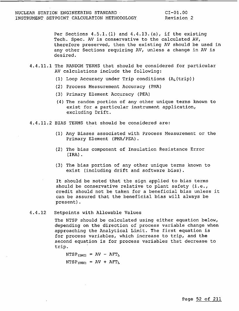
NUCLEAR STATION ENGINEERING STANDARD CI-01.00INSTRUMENT SETPOINT CALCULATION METHODOLOGY Revision 2
Per Sections 4.5.1.(l) and 4.4.13.(a), if the existingTech. Spec. AV is conservative to the calculated AV,therefore preserved, then the existing AV should be used inany other Sections requiring AV, unless a change in AV isdesired.
4.4.11.1 The RANDOM TERMS that should be considered for particularAV calculations include the following:
(1) Loop Accuracy under Trip conditions (AL(trip))
(2) Process Measurement Accuracy (PMA)
(3) Primary Element Accuracy (PEA)
(4) The random portion of any other unique terms known toexist for a particular instrument application,excluding Drift.
4.4.11.2 BIAS TERMS that should be considered are:
(1) Any Biases associated with Process Measurement or thePrimary Element (PMA/PEA).
(2) The bias component of Insulation Resistance Error(IRA).
(3) The bias portion of any other unique terms known toexist (including drift and software bias).
It should be noted that the sign applied to bias termsshould be conservative relative to plant safety (i.e.,credit should not be taken for a beneficial bias unless itcan be assured that the beneficial bias will always bepresent).
4.4.12 Setpoints with Allowable Values
The NTSP should be calculated using either equation below,depending on the direction of process variable change whenapproaching the Analytical Limit. The first equation isfor process variables, which increase to trip, and thesecond equation is for process variables that decrease totrip.
NTSP(INc) = AV - AFTL
NTSP(DEC) = AV + AFTL
Page 52 of 211
NUCLEAR STATION ENGINEERING STANDARDINSTRUMENT SETPOINT CALCULATION METHODOLOGY
CI-01.00Revision 2
4.4.12.1 Selecting Actual Setpoints
The actual setpoint used in calibrating instrumentationmay not be the value of the NTSP calculated. The choice ofthe actual setpoint to be used in the plant is a matter ofevaluating setpoint conservatism as compared to the AV andoperational preferences. In other words, the existingplant setpoint may be conservative to the calculatedsetpoint and AV and pose limited impact on plantoperations or spurious trips. This in-plant (existing)setpoint would satisfy both the calculation requirementsand plant operation, as such, the channel would notrequire a setpoint revision. The existing setpoint,becomes the NTSP and used in any other Sections requiringNTSP.Evaluation of Trip Reset Value
The reset setting is a variable % span adjustment of thetrip setpoint. CPS calibration procedures typically has itset at 3% span (i.e. Trip is set at 100%, reset is shown as97%). The same AFT and ALT is placed on the trip setpoint,as well as the reset, however, it is not possible for thetrip to be found low in it's band, while the reset is foundhigh. Areas to consider are as follows:
a. The loop has both a high and low setpoint, with theresets overlapping, thus potentially both alarms at
4.4. 12.2
the same time.b. When calculated AFT is greater than the reset in
calibration procedure.c. Both trip and reset require a NTSP calculation to
provide different functions.
The reset value may require adjustment different than thetypical setting of 3% span.
4.4.13 Evaluating Results and Resolving Problems
The evaluation of results depends to some extent on theultimate goal of the setpoint calculations. If there is noexisting setpoint in use no evaluation may be necessary.However, in the more normal case, there is already anexisting setpoint and, in some cases, TechnicalSpecifications requirements. In this case, the evaluationof results should include:
a. Evaluate the calculated Nominal Trip Setpoint andAllowable Value against existing values. If existingvalues are not supported by the calculations,determine whether or not it is desirable to preservethe existing values.
Page 53 of 211
NUCLEAR STATION ENGINEERING STANDARD CI-01.00INSTRUMENT SETPOINT CALCULATION METHODOLOGY Revision 2
b. If existing values are to be preserved, investigateiteration opportunities and revise the calculations.
4.4.13.1 Iteration to Resolve Setpoint Problems
There are usually opportunities for iteration as a meansof resolving problems with a calculated setpoint, short ofmodifying instrument installations or hardware. As aminimum, the following alternatives should be considered:
(1) Modify the Analytical Limit. Frequently, analysesthat are the source of the analytical limit havemargin. Changes to the analytical limit, to takecredit for existing analysis margins, is a powerfulway to optimize setpoint calculations, since it hasno impact on instrumentation or instrument errorallowances. Further, there are many situations (evenin plant transient or accident analyses) whererelatively simple parameter studies can be used toadjust the analytical limit without re-doing theactual transient or accident analyses.
(2) Re-evaluate environmental assumptions. Manyenvironmental assumptions are driven by worst caselicensing assumptions, which may not be appropriateto instrument error analyses. For example, it makesno sense to use an environment that assumes plantconditions that the instrument setpoint of interestis designed to prevent. Environmental assumptionsmay also be optimized by careful consideration oftrip timing, and by refining the analyses thatpredict environmental conditions.
(3) Re-evaluate calibration errors. Use of differentcalibration instruments, modified As-Found or As-LeftTolerances can be used to change calibration errorallowances and improve setpoint calculations.
(4) Re-evaluate drift assumptions. Consider usingstatistical analyses of actual as-found and as-leftdata from surveillance testing to justify improveddrift allowances.
(5) Evaluate other assumptions in setpoint calculations,such as function requirements for the instru-mentation, trip timing, surveillance intervals, etc.
(6) Examine instrument applications. For example, forsetpoints heavily impacted by a predicted radiationdose, a change from a standard model to a radiationresistant model of the same instrument can have majorbenefits (changing from a Rosemount 1153B "P" outputto an 1153B "R" output, for example).
Page 54 of 211
NUCLEAR STATION ENGINEERING STANDARD CI-01.00INSTRUMENT SETPOINT CALCULATION METHODOLOGY Revision 2
4.5 Calculation Nominal Trip Setpoints and Indication/ControlLoops
The individual calculations associated with setpoint andchannel error evaluations are outlined below. The engineerperforming the calculations should determine whichcalculations apply to the particular situation, based onthe guidance provided.
4.5.1 Setpoint with Analytical Limit
The following steps shall be performed for a Setpoint withAnalytical Limit:
a. Calculate the individual device accuracy (Ai) perSection 4.3.1.
b. Calculate the individual device As-Left Tolerance(ALTi) per Section 4.3.3.
c. Calculate the loop As-Left Tolerance (ALTL) per Section4.4.2.
d. Calculate the individual device Calibration Error (Ci)per Section 4.3.3.
e. Calculate the loop Calibration Error (CL) per Section4.4.3.
f. Calculate the individual device drift error (Di) perSections 4.3.2.
g. Calculate the loop Drift Error (DL) per Section 4.4.4
h. Calculate the individual device As-Found Tolerance(AFTi) per Section 4.3.3.
i. Calculate the loop As-Found Tolerance (AFTL) perSection 4.4.5
j. Develop PMA, PEA, IRA, and other error terms perSections 4.4.6 and 4.4.7 as applicable.
k. Calculate the Allowable Value (AV) from the AnalyticalLimit (AL) per Sections 4.4.10 and 4.4.11.
1. Compare calculated Allowable Value to existingTechnical Specification AV. Use the existing AV ifconservative, unless it is desired to revise theexisting Technical Specifications.
m. Calculate the Nominal Trip Setpoint (NTSP) from theAllowable Value per Section 4.4.12.
n. Consider whether adequate separation exists between theNominal Trip Setpoint and Allowable Value to avoidLERs.
Page 55 of 211
NUCLEAR STATION ENGINEERING STANDARD CI-01.00INSTRUMENT SETPOINT CALCULATION METHODOLOGY Revision 2
o. Use the existing setpoint if conservative, unless it isdesired to revise it. Then select a setpoint to be usedin the calibration procedure that is bounded by theNominal Trip Setpoint.
p. Evaluate the Trip Reset Value
q. Optimize calculations, if necessary, to validateexisting Technical Specifications, designs, etc.
4.5.2 Indication/Control Loop
The following steps shall be performed for aIndication/Control Loop:
a. Calculate values per Section 4.5.1.a through 4.5.1.j.b. Calculate the channel uncertainty (CU) and channel error
(CE) per Section 4.4.8.
c. Optimize calculations, if necessary, to validateexisting Technical Specifications, designs, etc.
Note: If indication loop also provides indication for aspecific reading as required by the Tech. Spec, thensections 4.5.1.k through 4.5.1.o should be addressed forthat indicated reading (in lieu of setpoint).
4.5.3 Setpoint without Analytical Limit
The following steps shall be performed for Setpoint withoutAnalytical Limit:
a. Calculate values per Section 4.5.1.a through 4.5.1.j.
b. Calculate the channel uncertainty (CU) and channel error(CE) per Section 4.4.8.
c. Identify the Nominal Process Limit (NPL) per Section4.4.9. This also might be given as an Allowable value.
d. Calculate the Nominal Trip Setpoint (NTSP) from theNominal Process Limit using the channel error perSection 4.4.9.
e. Use the existing setpoint if conservative, unless it isdesired to revise it. Then select a setpoint to be usedin the calibration procedure that is bounded by theNominal Trip Setpoint.
f. Optimize calculations, if necessary, to validateexisting designs, etc.
Page 56 of 211
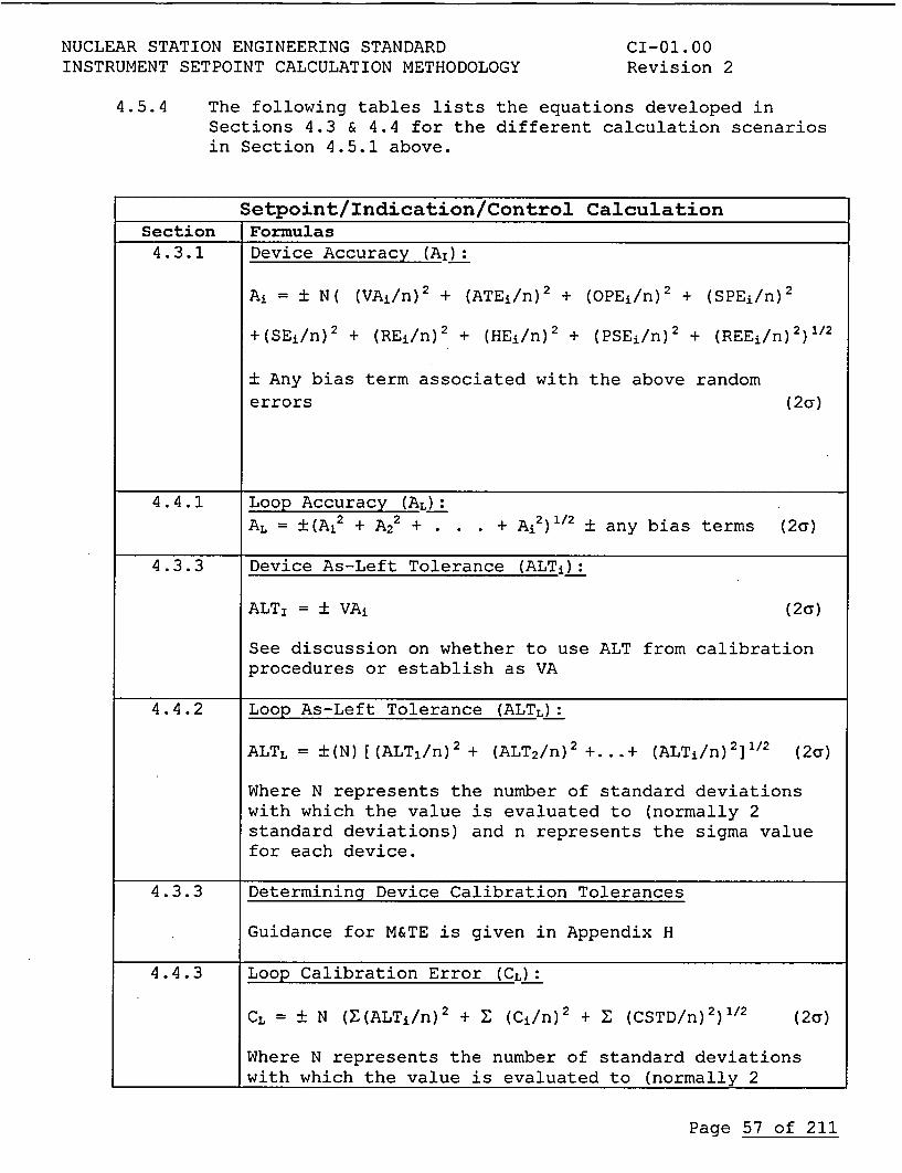
NUCLEAR STATION ENGINEERING STANDARDINSTRUMENT SETPOINT CALCULATION METHODOLOGY
CI-01.00Revision 2
4.5.4 The following tables lists the equations developed inSections 4.3 & 4.4 for the different calculation scenariosin Section 4.5.1 above.
Setpoint/Indication/Control CalculationSection Formulas4.3.1 Device Accuracy (A,)
Ai = ± N( (VAi/n)2 + (ATEi/n)2 + (OPEi/n)2 + (SPEi/n)2
+(SEi/n)2 + (REi/n) 2 + (HE,/n) 2 + (PSE1 /n) 2 + (REEi/n) 2 )1 /2
± Any bias term associated with the above randomerrors (2a)
4.4.1 Loop Accuracy (AL):AL = +(Al2 + A2
2 + . . . + A 12 ) 1 / 2 ± any bias terms (2a)
4.3.3 Device As-Left Tolerance (ALTi):
ALT, = + VAi (2a)
See discussion on whether to use ALT from calibrationprocedures or establish as VA
4.4.2 Loop As-Left Tolerance (ALTL):
ALTL = (N)[(ALT 1/n)2 + (ALT2/n) 2 +.+ (ALTi/n) 2 ] 1/2 (2a)
Where N represents the number of standard deviationswith which the value is evaluated to (normally 2standard deviations) and n represents the sigma valuefor each device.
4.3.3 Determining Device Calibration Tolerances
Guidance for M&TE is given in Appendix H
4.4.3 Loop Calibration Error (CL):
CL = ± N (Z(ALTi/n)2 + X (Ci/n) 2 + X (CSTD/n)2)11 2 (2a)
Where N represents the number of standard deviationswith which the value is evaluated to (normally 2
Page 57 of 211
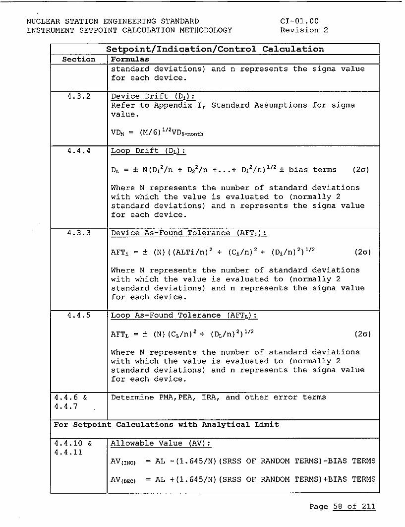
NUCLEAR STATION ENGINEERING STANDARDINSTRUMENT SETPOINT CALCULATION METHODOLOGY
CI-01.00Revision 2
Setpoint/Indication/Control CalculationSection Formulas
standard deviations) and n represents the sigma valuefor each device.
4.3.2 Device Drift (Di):Refer to Appendix I, Standard Assumptions for sigmavalue.
VDM = (M/6)1 /2VD6-month
4.4.4 Loop Drift (DL):
DL = ± N(D12/n + D22/n +...+ D,2/n) bias terms (2a)
Where N represents the number of standard deviationswith which the value is evaluated to (normally 2standard deviations) and n represents the sigma valuefor each device.
4.3.3 Device As-Found Tolerance (AFTi):
AFTi = ± (N) ((ALTi/n)2 + (Ci/n) 2 + (Di/n)2)1/2 (2a)
Where N represents the number of standard deviationswith which the value is evaluated to (normally 2standard deviations) and n represents the sigma valuefor each device.
4.4.5 Loop As-Found Tolerance (AFTL):
AFTL = ± (N) (CL/n) 2 + (DL/n) 2) 1/2 (2a)
Where N represents the number of standard deviationswith which the value is evaluated to (normally 2standard deviations) and n represents the sigma valuefor each device.
4.4.6 & Determine PMA,PEA, IRA, and other error terms4.4.7
For Setpoint Calculations with Analytical Limit
4.4.10 & Allowable Value (AV):4.4.11
AV(INC) = AL -(1.645/N) (SRSS OF RANDOM TERMS)-BIAS TERMS
AV(DEC) = AL +(1.645/N) (SRSS OF RANDOM TERMS)+BIAS TERMS
Page 58 of 211
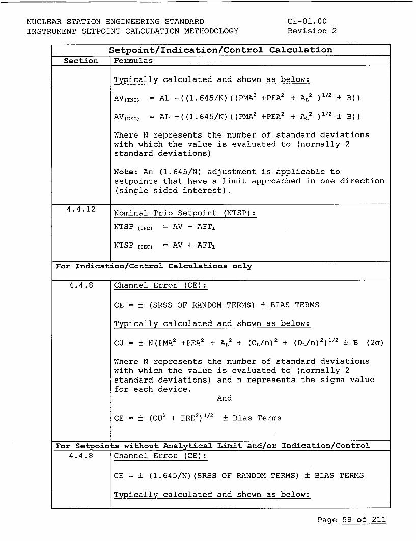
NUCLEAR STATION ENGINEERING STANDARDINSTRUMENT SETPOINT CALCULATION METHODOLOGY
CI-01. 00Revision 2
Setpoint/Indication/Control CalculationSection Formulas
4-
Typically calculated and shown as below:
AV(INC) = AL -((1.645/N) ( (PMA2 +PEA2 + AL2 ) 1/2 ± B) )
AV(DEC) = AL +((1.645/N)((PMA2 +PEA2 + A2 ) 1/2 ± B) )
Where N represents the number of standard deviationswith which the value is evaluated to (normally 2standard deviations)
Note: An (1.645/N) adjustment is applicable tosetpoints that have a limit approached in one direction(single sided interest).
4.4.12 Nominal Trip Setpoint (NTSP):
NTSP (INC) = AV - AFTL
NTSP (DEC) = AV + AFTL
For Indication/Control Calculations only
4.4.8 Channel Error (CE):
CE = ± (SRSS OF RANDOM TERMS) ± BIAS TERMS
Typically calculated and shown as below:
CU = ± N(PMA2 +PEA2 + AL2 + (CL/n) 2 + (DL/n) 2 ) 1 / 2 ± B (2a)
Where N represents the number of standard deviationswith which the value is evaluated to (normally 2standard deviations) and n represents the sigma valuefor each device.
And
CE ± (CU2 + IRE 2 ) 1 /2 ± Bias Terms
For Setpoints without Analytical Limit and/or Indication/Control4.4.8 Channel Error (CE):
CE = ± (1.645/N) (SRSS OF RANDOM TERMS) + BIAS TERMS
Typically calculated and shown as below:
Page 59 of 211
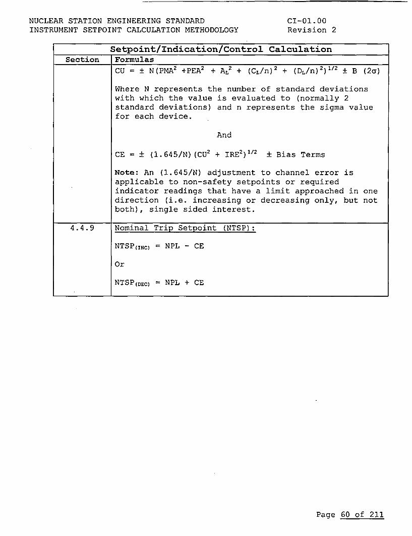
NUCLEAR STATION ENGINEERING STANDARDINSTRUMENT SETPOINT CALCULATION METHODOLOGY
CI-01.00Revision 2
Setpoint/Indication/Control CalculationSection jFormulas
CU = ± N(PMA2 +PEA2 + AL2 + (CL/n)2 + (DL/n)2) 1/2 ± B (2a)
Where N represents the number of standard deviationswith which the value is evaluated to (normally 2standard deviations) and n represents the sigma valuefor each device.
And
CE = ± (1.645/N) (CU2 + IRE2)1I 2 + Bias Terms
Note: An (1.645/N) adjustment to channel error isapplicable to non-safety setpoints or requiredindicator readings that have a limit approached in onedirection (i.e. increasing or decreasing only, but notboth), single sided interest.
4.4.9 Nominal Trip Setpoint (NTSP):
NTSP(INC) = NPL - CE
Or
NTSP(DEC) = NPL + CE
Page 60 of 211
NUCLEAR STATION ENGINEERING STANDARD CI-01.00INSTRUMENT SETPOINT CALCULATION METHODOLOGY Revision 2
5.0 REFERENCES
5.1 NEDC-31336, General Electric Improved Setpoint Methodology,October 1986, (GE Proprietary information)
5.2 Deleted
5.3 Industry Standard ANSI/ISA Standard S67.04, Setpoints forNuclear safety Related Instrumentation Parts I and II
And,
ISA dTR 67.04.09, Graded Approaches to SetpointDetermination, Draft Technical Report, 1994 and thesubsequent version Draft 4, May, 2000
5.4 GE Nuclear Energy internal procedures
5.5 General Electric Document EDE-40-1189 (Rev. 0)
5.6 ANS/ASME PTC 19.1-1985, Measurement Uncertainty
Establishes a basis for the principles of uncertaintyanalysis.
5.7 ASME MFC-3M-1989, Measurement of fluid Flow in Pipes UsingOrifice, Nozzle, and Venturi
Provides information regarding expected uncertainties anderrors associated with flow measurement.
5.8 ASME 1967 Steam Tables
Provides the basis for water density as a function oftemperature and pressure. When used, the appropriatepages should be copied and made as an attachment to thecalculation.
5.9 ANSI N42.18, American National Standard for Specificationand Performance of On-Site Instrumentation forContinuously Monitoring Radioactivity in Effluents
This standard establishes minimum expected performancestandards for certain types of radiation monitoringequipment.
5.10 The Institute for Nuclear Power Operations (INPO) GoodPractice TS-405, Setpoint Change Control Program.
Provides guidance for setpoint change control andimplementation practice.
Page 61 of 211
NUCLEAR STATION ENGINEERING STANDARD CI-01.00INSTRUMENT SETPOINT CALCULATION METHODOLOGY Revision 2
5.11 Regulatory Guide 1.105, Rev. 01, Setpoints for Safety-Related Instrumentation
CPS has committed to Regulatory Guide 1.105 Rev 01 forguidance relative to instrument setpoint preparation andcontrol. This Regulatory Guide 1.105 establishes theNRC's proposed endorsement of the ISA-67.04. Thediscussion also provides the NRC's perspective on varioustechnical areas related to setpoint methodologies andstatistical analysis.
5.12 NRC Information Notice 92-12, Effects of Cable LeakageCurrents on Instrument Settings and indications
Information Notice 92-12 describes a potential problemrelated to instrument loop current leakage. During thehigh humidity and temperature conditions of a LOCA orHELB, insulation resistance can be degraded, therebycontributing to the measurement uncertainty of affectedinstrument loops.
5.13 Not Used
5.14 CPS 1512.01, Rev. 17b, Calibration and Control ofMeasuring and Test Equipment (M&TE) and CPS 1012.01,Rev.9, Control of Measuring and Test Equipment.
These procedures establish generic requirements andcontrols for calibration and verification of TestEquipment and Reference Standards. Additionally, theadministrative requirements for controlling M&TE areprovided. These procedures establish the minimumrequirements for M&TE control. This Engineering Standardassumes that M&TE is controlled in accordance with thisdirective.
5.15 CPS 8801.01, Rev. 12b, Instrument Calibrations
This procedure provides instructions for performingoperations verification and calibration of single andmultiple input devices as an individual instrument. Italso includes instructions for development of InstrumentData Sheets.
5.16 CPS 8801.02, Rev. Ila, Loop Calibrations
This procedure provides instructions for performingoperations verification and calibration of instrumentloops. It also includes instructions for development ofLoop Calibration Data Sheets.
Page 62 of 211
NUCLEAR STATION ENGINEERING STANDARD CI-01.00INSTRUMENT SETPOINT CALCULATION METHODOLOGY Revision 2
5.17 CPS 8801.05, Rev. 5, Corrections to InstrumentCalibrations
This procedure provides instructions for scaling andapplying corrections to setpoint data obtained fromEngineering.
5.18 Not Used
5.19 Not Used
5.20 Not Used
5.21 NSED E.1, Rev. 10, Calculations
This procedure establishes generic requirements andcontrols for preparation, review, documentation andapproval of design calculations.
5.22 Calculation 01ME127, Rev.0, DBA Influence On Insulation-Resistance Related Instrument Errors
This calculation determines the influence of design basisaccident (DBA) conditions on containment instrumentationloop signal transmission systems (i.e., penetrations,cabling, splices, and conduit seals) and the consequenteffect on the accuracy of measurement of safety-relatedprocess parameters. The calculation addresses thoseinstrument loops which have the primary devices locatedinside containment and for which S&L has preparedinstrument setpoint accuracy calculations per therequirements of Reg. Guide 1.105.
5.23 Calculation 01ME128, Rev. 0, DBA Influence On Insulation-Resistance Related Instrument Errors For GE RG 1.105Instruments
This calculation determines the influence of design basisaccident (DBA) conditions on containment instrumentationloop signal transmission systems (i.e., penetrations,cabling, splices, and conduit seals) and the consequenteffect on the accuracy of measurement of safety-relatedprocess parameters. The calculation addresses thoseinstrument loops which have the primary devices locatedinside containment and for which GE has prepared instrumentsetpoint accuracy calculations per the requirements of RG1.105.
Page 63 of 211
NUCLEAR STATION ENGINEERING STANDARD CI-01.00INSTRUMENT SETPOINT CALCULATION METHODOLOGY Revision 2
5.24 Calculation CI-CPS-187, Rev. 0, DBA Influence OnInsulation-Resistance Related Instrument Errors
This calculation provides similar information asCalculations 01ME127 or 01ME128. Also, this calculationdetermines the bounding influence on instrumentation loopsfor each generic circuit type (current source, voltagesource, and bridge current source), that can be applied tosimilar circuits under harsh conditions. This calculationaddresses instrument loops that have the primary deviceslocated outside containment and for which Sargent & Lundyprepared Reg. Guide 1.105 instrument setpointcalculations.
5.25 Not Used
5.26 Not Used
5.27 Not Used
5.28 Honeywell 4450 Extended Analog System Input 4400 AG-T,Termination Assembly, K2801-0116A, Tab 15, and Analog InputSubsystem, K2801-0116B, Book 1, Tab 2.
Vendor Manual and Specifications
5.29 Record of Teleconference from Carl M. Ingram to J. Miller.
File Nos. 126.5, S/U 33.1. 10/16/81
Computer Point Accuracy and digital gain error.
5.30 IP-C-0089 Rev. 0, "M&TE Uncertainty Calculation"
5.31 ASTM Standard D257-91, Standard Test Methods for D-CResistance or Conductance of Insulating Materials, AppendixXI
5.32 EPRI TR-103335, Rev. 1, Statistical Analysis of InstrumentCalibration Data.
5.33 EPRI TR-102644, Calibration of Radiation Monitors atNuclear Power Plants
5.34 Regulatory Guide 1.97, Rev. 3, Instrumentation for Light-Water-Cooled Nuclear Power Plants to Assess Plant andEnvirons Conditions During and Following an Accident.
5.35 Regulatory Guide 1.89, Rev. 0, Qualification of Class lEEquipment For Nuclear Power Plants
5.36 DC-ME-09-CP, Rev. 11, "Equipment Environmental DesignConditions, Design Criteria."
5.37 CPS 1003.09, Rev. Oa, "CPS Instrument Setpoint ProgramInterfaces"
Page 64 of 211
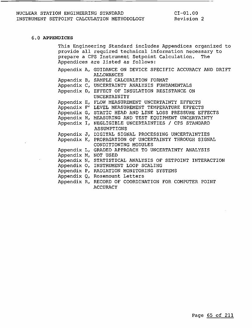
NUCLEAR STATION ENGINEERING STANDARDINSTRUMENT SETPOINT CALCULATION METHODOLOGY
CI-01.00Revision 2
6.0 APPENDICES
This Engineering Standard includes Appendices organized toprovide all required technical information necessary toprepare a CPS Instrument Setpoint Calculation. TheAppendices are listed as follows:
Appendix A,
AppendixAppendixAppendix
AppendixAppendixAppendixAppendixAppendix
AppendixAppendix
AppendixAppendixAppendixAppendixAppendixAppendixAppendix
B,C,D,
E,F'G.H,I,
J.K,
L,M,N,0,P.
Q.R.
GUIDANCE ON DEVICE SPECIFIC ACCURACY AND DRIFTALLOWANCESSAMPLE CALCUALTION FORMATUNCERTAINTY ANALYSIS FUNDAMENTALSEFFECT OF INSULATION RESISTANCE ONUNCERTAINITYFLOW MEASUREMENT UNCERTAINTY EFFECTSLEVEL MEASUREMENT TEMPERATURE EFFECTSSTATIC HEAD AND LINE LOSS PRESSURE EFFECTSMEASURING AND TEST EQUIPMENT UNCERTAINTYNEGLIGIBLE UNCERTAINTIES / CPS STANDARDASSUMPTIONSDIGITAL SIGNAL PROCESSING UNCERTAINTIESPROPAGATION OF UNCERTAINTY THROUGH SIGNALCONDITIONING MODULESGRADED APPROACH TO UNCERTAINTY ANALYSISNOT USEDSTATISTICAL ANALYSIS OF SETPOINT INTERACTIONINSTRUMENT LOOP SCALINGRADIATION MONITORING SYSTEMSRosemount LettersRECORD OF COORDINATION FOR COMPUTER POINTACCURACY
Page 65 of 211
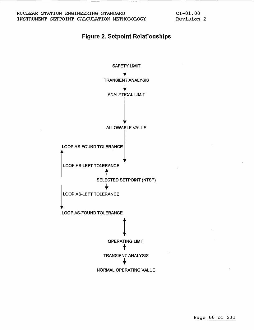
NUCLEAR STATION ENGINEERING STANDARD CI-01.00INSTRUMENT SETPOINT CALCULATION METHODOLOGY Revision 2
Figure 2. Setpoint Relationships
SAFETY LIMIT
TRANSIENT ANALYSIS
ANALYTICAL LIMIT
ALLOWABLE VALUE
LOOP AS-FOUND TOLERANCE
LOOP AS-LEFT TOLERANCE
tSELECTED SETPOINT (NTSP)
LOOP AS-LEFT TOLERANCE
LOOP AS-FOUND TOLERANCE
OPERATING LIMIT
TRANSIENT ANALYSIS
NORMAL OPERATING VALUE
Page 66 of 211
INSTRUMENT SETPOINT APPENDIX A GUIDANCE ON DEVICECALCULATION METHODOLOGY SPECIFIC ACCURACY AND DRIFT ALLOWANCESRevision 2
APPENDIX A
GUIDANCE ON DEVICE SPECIFIC ACCURACY AND DRIFT ALLOWANCES
A.1 Overview
In general, there are three parameters relating to Accuracy andDrift, which must be determined for any given device. These areAccuracy under normal conditions (Ai(normal)), Accuracy under tripconditions (Ai(trip)) and Drift (Di). There are two steps that mustbe taken to determine these values.
a. Identify the individual effects that may contribute to theseerrors.
b. Obtain numerical data on the identified individual effects.
In determining the effects that may contribute, and identify thenumerical values, consideration should be given to the followingsources of information (in order of importance):
c. Clinton specific data from testing of actual instruments,surveillance records, qualification programs, etc.
d. Generic data from testing of actual instruments, surveillancedata, qualification programs, etc.
e. Vendor supplied data sheets and data.
f. Purchase specifications for equipment
g. Generally accepted assumptions.
The purpose of this appendix is to provide guidance for the processdescribed above.
Page 67 of 211
INSTRUMENT SETPOINTCALCULATION METHODOLOGYRevision 2
APPENDIX A GUIDANCE ON DEVICESPECIFIC ACCURACY AND DRIFT ALLOWANCES
A.2 Effects Expected to be Present in Accuracy and DriftValues
AccuracyA.2.1
As discussed in paragraph 4.3.1 and defined in Section 2.2, thefollowing effects may typically be part of instrument accuracy(potentially, for both normal and trip conditions):
a. Vendor Accuracy (VA)
b. Accuracy Temperature Effect (ATE)
c. Overpressure Effect (OPE)
d. Static Pressure Effect (SPE)
e. Seismic Effect (SE)
f. Radiation Effect (RE)
g. Humidity Effect (HE)
h. Power Supply Effect (PSE)
i. RFI/EMI Effect (REE)
It may not be possible, in many cases, to determine all of theabove effects. Qualification testing, or vendor performancespecifications may simply state a value for accuracy, and thenstipulate a range of temperatures, radiation levels, seismic loads,humidity and other boundaries within which the value of accuracy isapplicable. In such cases, there is no need to determine theseparate effects.
A.2.1.a Rosemount Transmitter Devices
In the absence of suitable vendor data, Clinton specificqualification data or surveillance test data GE recommends that theinformation in the following paragraphs be used. For a selectedgroup of Rosemount devices GE has determined recommended accuracyassumptions based on generic qualification testing. Thisinformation has been provided to the USNRC (Reference 2.1) and usedfor many setpoint calculations accepted by the NRC.
Page 68 of 211
INSTRUMENT SETPOINT APPENDIX A GUIDANCE ON DEVICECALCULATION METHODOLOGY SPECIFIC ACCURACY AND DRIFT ALLOWANCESRevision 2
A.2.1.a(l) Rosemount Transmitters
GE recommends that the following be used as a basis for determiningnormal and trip environment accuracies for Rosemount transmitters(models 1151, 1152-T0280, 1153 Series B, and 1154).
A.2.1.a.(1).(a) Vendor Accuracy (VA), Accuracy Temperature Effect(ATE), Power Supply Effect (PSE), Humidity Effect (HE) and RFI/EMIEffect (REE)
VA = 0.25% SP (3 Sigma)
ATE = (0.75% UR + 0.5% SP) (delta Ta)/100 (3 Sigma)
(double this value for Range Code 3)
PSE = 0.005% SP per volt (3 Sigma)
HE = 0 (included in VA)
REE = 0 (Normally negligible)
Determination of 'delta Ta' is discussed in paragraph A.2.3.
A.2.1.a.(1).(b) Overpressure Effect (OPE)
This effect varies depending on the instrument range, and isidentified in Rosemount product data sheets. GE treats theresulting values as 3 Sigma values based on experience with theRosemount data.
A.2.1.a.(l).(c) Static Pressure Effect (SPE)
As discussed in paragraph 4.3.1, SPE sometimes consists of severaleffects, some of which are random and some of which are bias. Thisis particularly the case with Rosemount differential pressuretransmitters (note, SPE does not apply to absolute pressure or gagepressure transmitters). In the case of Rosemount transmitters,there are three SPE components: (1) a random zero point error, (2)a random span error, and (3) a bias span error. The bias spanerror is easily adjusted for as part of the calibration process(this is often done). If accommodated in the calibration process,it need not be included in the accuracy error calculations.
GE has found that the Rosemount manuals may be difficult tointerpret concerning SPE. For this reason, the following summary isprovided to describe definition of the Rosemount SPE.
Page 69 of 211
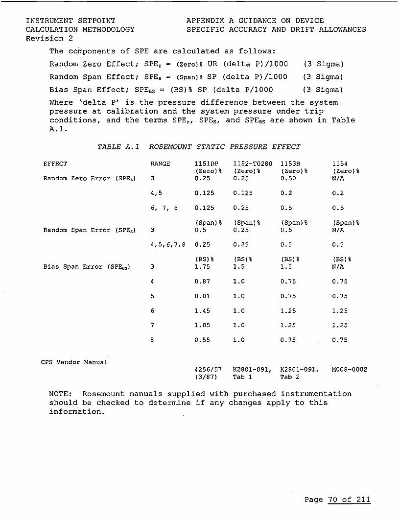
INSTRUMENT SETPOINTCALCULATION METHODOLOGYRevision 2
APPENDIX A GUIDANCE ON DEVICESPECIFIC ACCURACY AND DRIFT ALLOWANCES
The components of SPE are calculated as follows:
Random Zero Effect; SPEz = (Zero)% UR (delta P)/1000
Random Span Effect; SPE5 = (Span)% SP (delta P)/1000
Bias Span Effect; SPEBS = (BS)% SP (delta P/1000
(3 Sigma)
(3 Sigma)
(3 Sigma)
Where 'delta P' is the pressure difference between the systempressure at calibration and the system pressure under tripconditions, and the terms SPEz, SPEs, and SPEBs are shown in TableA.1.
TABLE A.1 ROSEMOUNT STATIC PRESSURE EFFECT
EFFECT RANGE
Random Zero Error (SPEz) 3
1151DP(Zero) %0.25
0.125
1152-T0280(Zero) %0.25
0.125
1153B(Zero) %0.50
1154(Zero) %N/A
4,5 0.2 0.2
6, 7, 8 0.125 0.25 0.5 0.5
(Span)% (Span)%3 0.5 0.25
(Span) %0.5
(Span) %N/ARandom Span Error (SPEs)
4,5,6,7,8 0.25
(BS) %1.75Bias Span Error (SPEas) 3
4
5
6
7
8
0.87
0.81
1.45
1.05
0.55
0.25
(BS) %1.5
1.0
1.0
1.0
1.0
1.0
0.5
(BS) %1.5
0.75
0.75
1.25
1.25
0.75
0.5
(BS)%N/A
0.75
0.75
1.25
1.25
0.75
CPS Vendor Manual4256/57 K2801-091,(3/87) Tab 1
K2801-091,Tab 2
M008-0002
NOTE: Rosemount manuals supplied with purchased instrumentationshould be checked to determine if any changes apply to thisinformation.
Page 70 of 211
INSTRUMENT SETPOINT APPENDIX A GUIDANCE ON DEVICECALCULATION METHODOLOGY SPECIFIC ACCURACY AND DRIFT ALLOWANCESRevision 2
A.2.1.a.(1).(d) Seismic Effect (SE)
Based on an evaluation of Rosemount test data, GE recommends thefollowing:
SE = 0.23% UR (2 Sigma)
Where equation applies to situations in which the Zero PeriodAcceleration (ZPA) at the mounting location of the transmitter doesnot exceed 1 "g" for the event of interest, and where thetransmitter is expected to be performing its trip functionsimultaneous with the seismic event.
SE = (0.03 ZPA + 0.20)% UR (2 Sigma)
Where ZPA exceeds 1 "g", but not 10 "g", and the transmitter isexpected to be performing its trip function simultaneous with theseismic event.
SE = 0.25% UR (2 Sigma)
Where ZPA exceeds 2 "g", but the seismic event is expected to occurbetween the time of the last calibration and the time of trip, butnot simultaneously.
If the seismic event ZPA does not exceed 2 "g", and the event isnot simultaneous with the trip event, the effect on transmitteraccuracy is negligible.
A.2.1.a.(1).(e) Radiation Effect (RE)
GE does not recommend use of Rosemount model 1151 transmitters fortrip applications for which the gamma Total Integrated Dose (TID)to time of trip exceeds approximately 104 RAD. Up to this value,the radiation effect on 1151 transmitters is negligible (plantspecific EQ program data should be used to support use of 1151transmitters in a radiation environment, if such data isavailable).
For the 1152-T0280 transmitter:
RE = (1.25X + 1.25)% UR (2 Sigma)
Where TID exceeds 0.1 MRAD, but does not exceed 0.4 MRAD. Thiseffect should be multiplied by 1.68 for Range Code 3. There is noeffect at or below 0.1 MRAD.
RE = (4.5X + 4.5)% UR (2 Sigma)
Where TID exceeds 0.4 MRAD, but not 20 MRAD. This effect shouldalso be multiplied by 1.68 for Range Code 3.
Page 71 of 211
INSTRUMENT SETPOINT APPENDIX A GUIDANCE ON DEVICECALCULATION METHODOLOGY SPECIFIC ACCURACY AND DRIFT ALLOWANCESRevision 2
The term "X" is defined as:
X = (setpoint of interest-instrument zero)/calibrated span
For the 1153 Series B transmitter with a "P" output:
RE = (3.OX + 3.0)% UR (2 Sigma)
Where TID exceeds 0.1 MRAD, but not 22 MRAD. There is no effect ator below 0.1 MRAD. This effect should also be multiplied by 1.68for Range Code 3.
For the 1153 Series B transmitter with an "R" output:
RE = (1.5X + 1.5)% UR (2 Sigma)
Where TID exceeds 0.1 MRAD, but not 22 MRAD. There is no effect ator below 0.1 MRAD. This effect should also be multiplied by 1.68for Range Code 3.
For the 1154 transmitter:
RE = (1.0X + 1.0)% UR (2 sigma)
Where TID exceeds 0.5 MRAD, but not 50 MRAD. There is no effect ator below 0.5 MRAD. This effect should also be multiplied by 1.68for Range Code 3.
A.2.1.a.(2) Rosemount Trip Units
For unmodified Rosemount model 510DU and 710DU trip units usevendor specified data for instrument uncertainties. For trip unitsmodified by GE (model number 147D8505G005), use GE PerformanceSpecification 22A7866 for instrument uncertainties.
A.2.2 Drift
As discussed paragraph 4.3.2, there are two terms of interest indetermining device drift. These are Vendor Drift (VD) and sometime interval associated with VD(usually 6 months). These effectsshould be determined from vendor data, field data, or qualificationdata, if available.
A.2.2.a Rosemount Devices
For a selected group of Rosemount devices GE has determinedrecommended drift assumptions based on generic qualificationtesting. This information has been provided to the USNRC(Reference 5.1) and used for many setpoint calculations accepted bythe NRC. In the absence of suitable Clinton specific qualificationdata or surveillance test data GE recommends that the informationin the following paragraphs be used.
A.2.2.a.(1) Rosemount Transmitters
For Rosemount model 1151, 1152-T0280, 1153 Series B and 1154transmitters refer to vendor supplied information for theappropriate drift term. Due to Rosemount correspondences in theyear 2000, the Rosemount drift terms will conservatively beconsidered to be 2 sigma.
Page 72 of 211
INSTRUMENT SETPOINT APPENDIX A GUIDANCE ON DEVICECALCULATION METHODOLOGY SPECIFIC ACCURACY AND DRIFT ALLOWANCESRevision 2
A.2.2.a.(2) Rosemount Trip Units
For Rosemount model 510DU and 710DU trip units use the vendorspecified data. For trip units modified by GE (model number147D8505G005), use the GE Performance Specification 22A7866
A.2.3 (Deleted)
A.2.4 Interpreting Vendor Data
For many devices, it may be necessary to use vendor data sheets orspecifications as the source of accuracy and drift information forsetpoint calculations. However, vendors commonly use manydifferent terms to describe the performance of their equipment. Inaddition, most vendors do not specify their data in terms of aprobability of error (i.e., they don't say how many standarddeviations their values represent). Therefore, interpretation isnecessary.
When interpreting terminology, the definitions in Section 2.2 ofthis document should be used to ensure consistent interpretation.For example, the definition of Channel Instrument Accuracy,paragraph 2.2.11, states that accuracy, as referred to in the CPSSetpoint Methodology, includes "the combined conformity, hysteresisand repeatability errors". Paragraph 2.2.11 also indicates certainterms, which are not considered to be part of accuracy.
Care should be exercised to relate the vendor-defined errors to thefunctions of the instrument channel. For example, a Rosemount tripunit with an analog indicator has two distinct sets of errors.There are errors associated with the trip circuitry, and whichapply to a trip setpoint calculation. There are also errorsassociated with the analog indicator, which do not apply to thetrip function, but which would apply if the purpose of thecalculation is to define the error associated with readings takingusing the analog indicator.
In some cases, vendors may not identify all errors of interest.For some types of devices, vendors identify accuracy errors but nodrift effects. In such cases, it is necessary to first determinewhether or not there is satisfactory evidence that the omitted item(drift, for example) does not apply to this type of device. Ifavailable information is not convincing, it may be necessary toassume a value. Paragraphs A.2.5 and A.2.6 contain recommendationsfor establishing error terms on the basis of field data and/orconservative assumptions.
Page 73 of 211
INSTRUMENT SETPOINT APPENDIX A GUIDANCE ON DEVICECALCULATION METHODOLOGY SPECIFIC ACCURACY AND DRIFT ALLOWANCESRevision 2
The final aspect of importance when interpreting vendor data isdetermining how many standard deviations (sigma values) the datarepresents. In general, this is an issue of how much confidence wehave in the vendor data. Data may be qualitatively classified intothree categories: (1) best estimate data, (2) worst case datawhich is backed by limited testing, and (3) worst case data backedby extensive qualification testing or testing of every delivereddevice. In the absence of information from a vendor, whichspecifies the sigma value associated with the data, GE recommendstreating data as follows:
a. Best Estimates: Assume they are (1) sigma values.
b. Worst case data backed by limited testing: Assume two (2)sigma.
c. Worst case data extensively backed: Assume three (3) sigma.
Under normal circumstances, all vendor data will be one of thelatter two cases (i.e., 2 or 3 sigma). This is because mostvendors specify instrument performance in terms of guaranteedperformance. In order to guarantee performance, the vendor musthave considerable confidence in the data. A two (2) sigma valuecorresponds to a 95% probability value, while three (3) sigmacorresponds to slightly greater than 99%. Thus, assignment of thesigma value to be assumed in the calculations is a question of theconfidence placed in the vendor data.
A.2.5 Interpreting Surveillance Test Data
Surveillance test data can be a valuable source of information withwhich to improve the database and refine setpoint calculations.The primary use of surveillance test data is in validating and/orrefining drift assumptions, and in extending instrumentsurveillance intervals. The primary limitation associated with useof field data is that there must be a valid basis for assumptionsas to what the data contains. For example, surveillance data isnormally valid as a source of improved drift information, and maybe used to estimate other surveillance test related errors, but isnot a good source for validating accuracy assumptions. Instrumentaccuracies may be quite different under trip conditions than duringsurveillance testing.
The basic approach to use of surveillance test data is a three partapproach:
a. Define, in terms of the values of interest (drift, etc.), whatthe surveillance data represents, as a means of defining howyou will interpret the data.
b. Collect the surveillance data needed to provide a strongstatistical basis.
c. Perform a statistical analysis of the data, and establish thedesired values along with the associated sigma level for usein channel error calculations or setpoint calculations.
Page 74 of 211
INSTRUMENT SETPOINT APPENDIX A GUIDANCE ON DEVICECALCULATION METHODOLOGY SPECIFIC ACCURACY AND DRIFT ALLOWANCESRevision 2
The area of greatest potential benefit associated with surveillancetest data analyses are the use of test data to validate reduceddrift assumptions for existing surveillance test intervals, and theuse of the data to predict revised drift values for longersurveillance test intervals. This latter is particularly useful inpreparing justifications for temporary surveillance intervalextensions in order to avoid undesired plant shutdowns forsurveillance testing.
Detailed calculation models and methods for evaluating surveillancetest data are beyond the scope of this document. Standardstatistical methods may be used. In addition, References 5.1, 5.3,& 5.32 contain a detailed discussion of validating driftassumptions from surveillance test data.
A.2.6 Recommended Assumptions in the Absence of DataIn the absence of better information, GE recommends the followingassumptions be used in channel error and setpoint calculations:a. Calibrating equipment accuracies are taken as 3 sigma values
provided that the calibration of these devices is to NISTtraceable standards and minimizes the effects of hysteresis,linearity and repeatability. The accuracies of the standardsthemselves are also taken to be 3 sigma values.
b. If Vendor Drift (VD) is not specified by the vendor oravailable from other sources, and if there is no basis forassuming drift is zero or negligible, assume VD equals VendorAccuracy (VA) over the entire calibration period.
A.2.7 Cautions Concerning Use of Qualification Program Data
Plant specific data from Equipment Qualifications programs is avaluable source of data on instrument performance, particularlyregarding the various accident related accuracy error terms(Radiation Effect, Seismic Effect, etc.). However, care should beexercised in use of this data.In many cases, Equipment Qualification programs have been conductedto prove that class IE equipment will function throughout itsintended lifetime. Because the post-accident functions includeindications for operator use, the environmental conditions used inEQ programs may include long term post-accident conditions, whichdo not apply to most setpoint calculations. Use of EQ results,without taking into account less severe trip conditions can resultin extreme conservatism. Overly conservative setpoints can impactplant operations and lead to unnecessary challenges to safetysystems.
Page 75 of 211
INSTRUMENT SETPOINTCALCULATION METHODOLOGY
APPENDIX B SAMPLE OF CALCULATION FORMATRevision 2
APPENDIX B
SAMPLE CALCULATION FORMAT
This sample presents, the format usedfor a selpoint and indication/controlcalculation. An Example of these types of calculations can be obtainedfrom theSetpoint Program Coordinator. The calculation cover sheets are produced usingE-1, Reference 5.21, Forms NF-161.01 through NF-161.04). The calculationshall reflect the name and order of major sections as shown in the TOC belowt,however, it is only recommended that sections within each major section bepresented as shown in this Attachment. For other types of calculations, such asNIs, A PRMs, and Radiation Monitors, the major sections of this sample should beused and Appendix Pfor guidance. The Setpoint Program Coordinator canprovide examples of what is shown within each major section.
TABLE OF CONTENTS
CALCULATION COVER SHEET ............................. (PAGE #)
REVISION HISTORY ......................... (PAGE #)
TABLE OF CONTENTS............................................................ (PAGE #)
1.0 OBJECTIVE .(PAGE #)
2.0 ASSUMPTIONS .(PAGE #)
3.0 METHODOLOGY .(PAGE #)
4.0 INPUTS .(PAGE #)
5.0 OUTPUTS .(PAGE #)
6.0 REFERENCES .(PAGE #)
7.0 ANALYSIS AND COMPUTATION SECTION(S) .(PAGE #)
8.0 RESULTS .(PAGE #)
9.0 CONCLUSIONS .(PAGE #)
ATTACHMENTS
ATTACHMENT 1, Scaling (# of pages)
ATTACHMENT 2, Results Summary (# of pages)
ATTACHMENT 3 (etc. as required) (# of pages)
Page 76 of 211
INSTRUMENT SETPOINT APPENDIX B SAMPLE OF CALCULATION FORMATCALCULATION METHODOLOGY Revision 2
1.0 OBJECTIVE
Should state purpose, finctions and objectives of calculation, including thecategory to which the amount of rigor is required.
2.0 ASSUMPTIONS
Other than CPS Standard Assumptions, there are two types that can be made: anassumption as to a value; or an assumption as to the quality of input information.For each assumption, a judgement must be made as to whether confirmation isrequired or justification is provided to show it is reasonable. Refer to NSED E.1,for further guidance.
All standard assumptions (See Appendix I, Section .11) required by thiscalculation wvill be listedfirst. Any additional assumptions as discussedabove, wvillfollow standard assumptions.
3.0 METHODOLOGY
Typical:This calculation will determine the instrument uncertainty associated with the(Function - Description). The evaluation will determine the loop setpoint andAllowable Value for the (Function). Instrument uncertainty will be determined inaccordance with CI-01.00, "Instrument Setpoint Calculation Methodology". Theevaluation will then compare the current setpoint and Allowable Value with theresults determined by this calculation.
M&TE error will be determined from the results of Calculation IP-C-0089,which uses building temperature minimum and maximums to develop theuncertainty, and review of the corresponding loop and device calibrationprocedures. Any changes to the calibration procedures will be shown inAttachment 2.
Per CI-01.00, Head Correction is determined by evaluating design drawings,survey data, and/or walk down data as applicable and calculated in Attachment 1.
Page 77 of 211
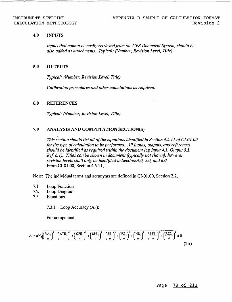
INSTRUMENT SETPOINTCALCULATION METHODOLOGY
APPENDIX B SAMPLE OF CALCULATION FORMATRevision 2
4.0 INPUTS
Inputs that cannot be easily retrievedfrom the CPS Document System, should bealso added as attachments. Typical: (Number, Revision Level, Title)
5.0 OUTPUTS
Typical: (Number, Revision Level, Title)
Calibration procedures and other calculations as required.
6.0 REFERENCES
Typical: (Nulmber, Revision Level, Title).
7.0 ANALYSIS AND COMPUTATION SECTION(S)
This section should list all of the equations identified in Section 4.5. 11 of CI-01. 00for the type of calculation to be performed. All inputs, outputs, and referencesshould be identified as required within the document (eg Input 4. 1, Output 5. 1,Ref 6. 1). Titles can be shown in document (typically not showvn), howeverrevision levels shall only be identified in Sections4. 0, 5. 0, and 6. 0.From CI-01.00, Section 4.5.11,
Note: The individual terms and acronyms are defined in CI-01.00, Section 2.2.
7.1 Loop Function7.2 Loop Diagram7.3 Equations
7.3.1 Loop Accuracy (AL):
For component,
_ N(~) +(ATh<) +(OP±)2 +(SP;)2 +(~.E)2 +(.I±)2 +(!!E) PS4
(2ar)
Page 78 of 211
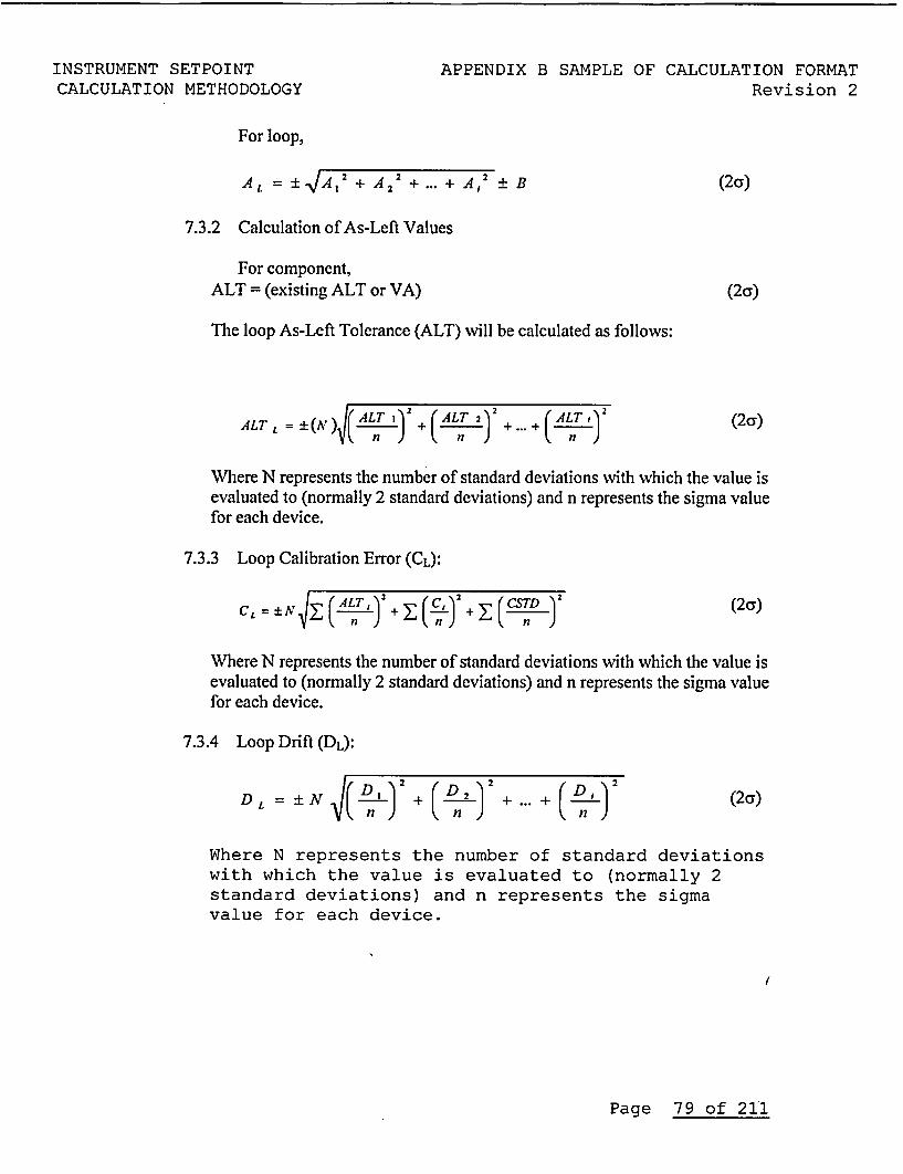
INSTRUMENT SETPOINTCALCULATION METHODOLOGY
APPENDIX B SAMPLE OF CALCULATION FORMATRevision 2
For loop,
AL = ± JA,2 + A 22 + ... + A, 2 ± B (2cr)
7.3.2 Calculation of As-Left Values
For component,ALT = (existing ALT or VA) (2c)
The loop As-Left Tolerance (ALT) will be calculated as follows:
ALT = (N(ALT+LT 2 + .. + ( ALT, ) (2a)
Where N represents the number of standard deviations with which the value isevaluated to (normally 2 standard deviations) and n represents the sigma valuefor each device.
7.3.3 Loop Calibration Error (CL):
CL = iN -y + Ad( + I'((2a)
Where N represents the number of standard deviations with which the value isevaluated to (normally 2 standard deviations) and n represents the sigma valuefor each device.
7.3.4 Loop Drift (DL):
D L=±NV(D )+ (D )+...+ ( ) (2a)
Where N represents the number of standard deviationswith which the value is evaluated to (normally 2standard deviations) and n represents the sigmavalue for each device.
Io
Page 79 of 211
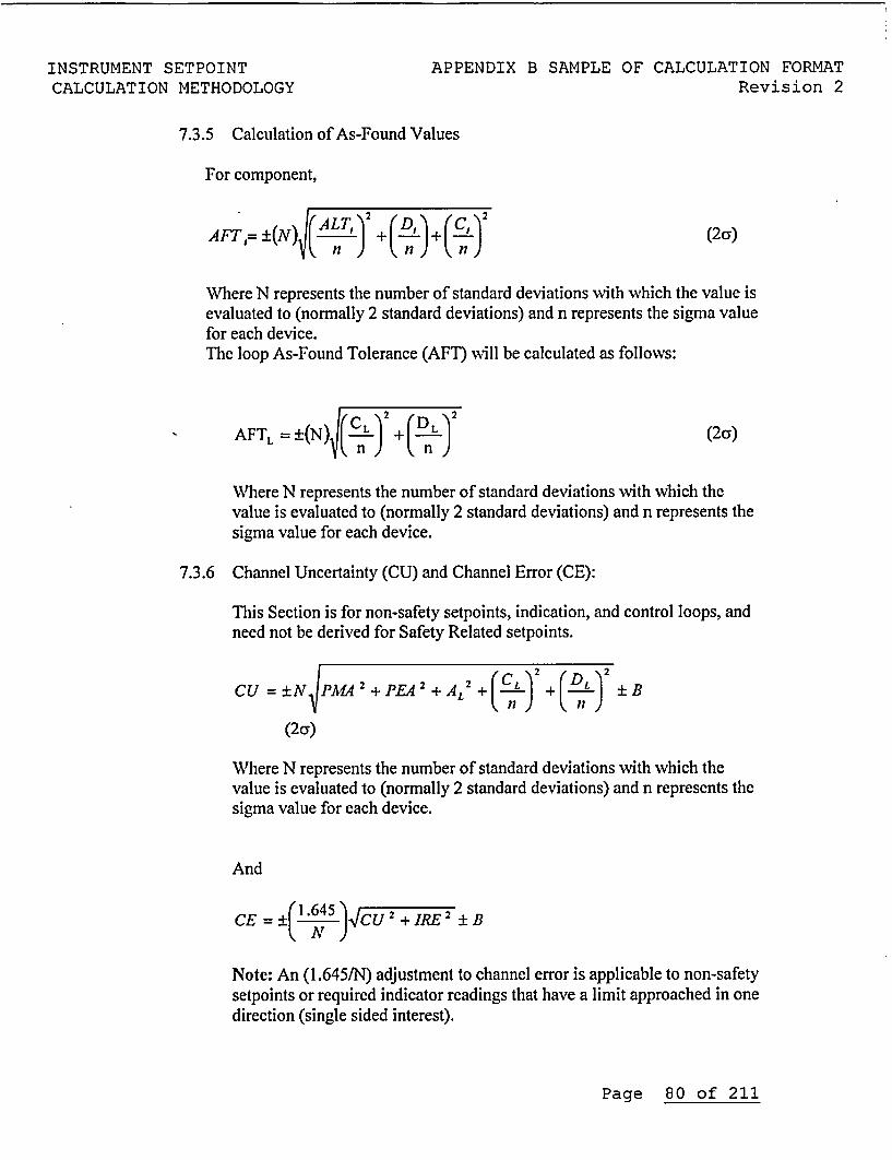
INSTRUMENT SETPOINT APPENDIX B SAMPLE OF CALCULATION FORMATCALCULATION METHODOLOGY Revision 2
7.3.5 Calculation of As-Found Values
For component,
AFT,= +(N)/( n ) +(D)J+[(§) (2a)
Where N represents the number of standard deviations with which the value isevaluated to (normally 2 standard deviations) and n represents the sigma valuefor each device.The loop As-Found Tolerance (AFT) will be calculated as follows:
AFTL =+(N) ) (DL ) (2a)
Where N represents the number of standard deviations with which thevalue is evaluated to (normally 2 standard deviations) and n represents thesigma value for each device.
7.3.6 Channel Uncertainty (CU) and Channel Error (CE):
This Section is for non-safety setpoints, indication, and control loops, andneed not be derived for Safety Related setpoints.
CU =±N ] +PEA +)AL J ( D ±B
(2cr)
Where N represents the number of standard deviations with which thevalue is evaluated to (normally 2 standard deviations) and n represents thesigma value for each device.
And
CE = i *5N CU 2 + IRE 2 iB
Note: An (1.645/N) adjustment to channel error is applicable to non-safetysetpoints or required indicator readings that have a limit approached in onedirection (single sided interest).
Page 80 of 211
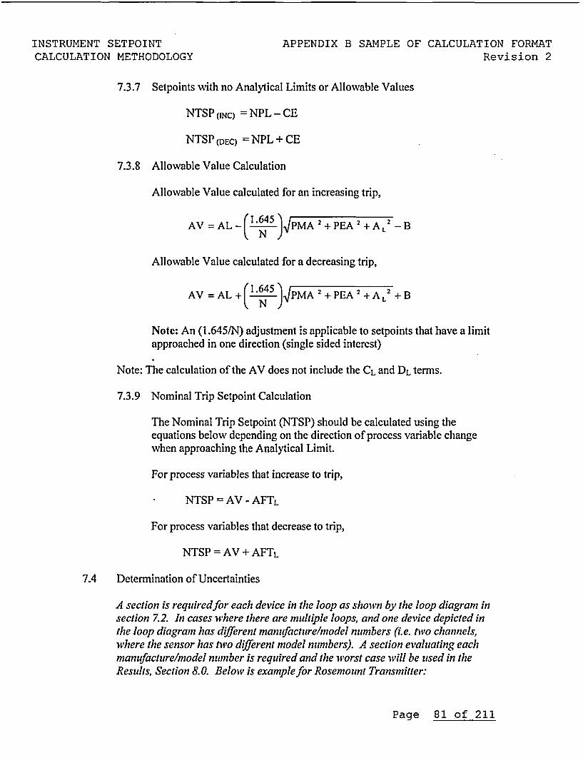
INSTRUMENT SETPOINT APPENDIX B SAMPLE OF CALCULATION FORMATCALCULATION METHODOLOGY Revision 2
7.3.7 Setpoints with no Analytical Limits or Allowable Values
NTSP (INC) = NPL - CE
NTSP (DEC) = NPL + CE
7.3.8 Allowable Value Calculation
Allowable Value calculated for an increasing trip,
AV =AL ( N )FPMA2 + PEA 2+AL2 B
Allowable Value calculated for a decreasing trip,
AV =AL+ (l N)IPMA2+PEA2+A L +B
Note: An (1.645/N) adjustment is applicable to setpoints that have a limitapproached in one direction (single sided interest)
Note: The calculation of the AV does not include the CL and DL terms.
7.3.9 Nominal Trip Setpoint Calculation
The Nominal Trip Setpoint (NTSP) should be calculated using theequations below depending on the direction of process variable changewhen approaching the Analytical Limit.
For process variables that increase to trip,
NTSP = AV - AFTL
For process variables that decrease to trip,
NTSP = AV + AFTL
7.4 Determination of Uncertainties
A section is requiredfor each device in the loop as shown by the loop diagram insection 7.2. In cases where there are multiple loops, and one device depicted inthe loop diagram has different manufacture/model numbers (i.e. tvo channels,where the sensor has two different model numbers). A section evaluating eachmanufacture/model number is required and the worst case will be used in theResults, Section 8. 0. Belowv is example for Rosemount Transmitter:
Page 81 of 211
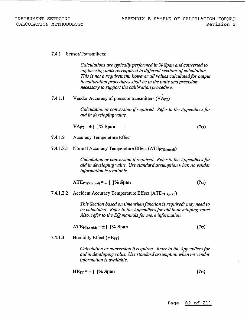
INSTRUMENT SETPOINT APPENDIX B SAMPLE OF CALCULATION FORMATCALCULATION METHODOLOGY Revision 2
7.4.1 Sensor/Transmitters;
Calculations are typically performed in % Span and converted toengineering units as required in different sections of calculation.This is not a requirement, however all values calculatedfor outputto calibration procedures shall be in the units andprecisionnecessary to support the calibration procedure.
7.4.1.1 Vendor Accuracy of pressure transmitters (VApT)
Calculation or conversion ifrequired. Refer to the Appendices foraid in developing value.
VAPT = ± I ]% Span (?a)
7.4.1.2 Accuracy Temperature Effect
7.4.1.2.1 Normal Accuracy Temperature Effect (ATEpT(NormaI))
Calculation or conversion ifrequired. Refer to the Appendices foraid in developing value. Use standard assumption when no vendorinformation is available.
ATErT(Normal)=± l I% Span (?a)
7.4.1.2.2 Accident Accuracy Temperature Effect (ATEPT(Accid))
This Section based on time when function is required; may need tobe calculated Refer to the Appendices for aid in developing value.Also, refer to the EQ manualsfor more information.
ATEPT(Accid) = ± I 1% Span (?ca)
7.4.1.3 Humidity Effect (HEpT)
Calculation or conversion ifrequired. Refer to the Appendices foraid in developing value. Use standard assumption when no vendorinformation is available.
HEpTr= ±i I% Span (?a)
Page 82 of 211
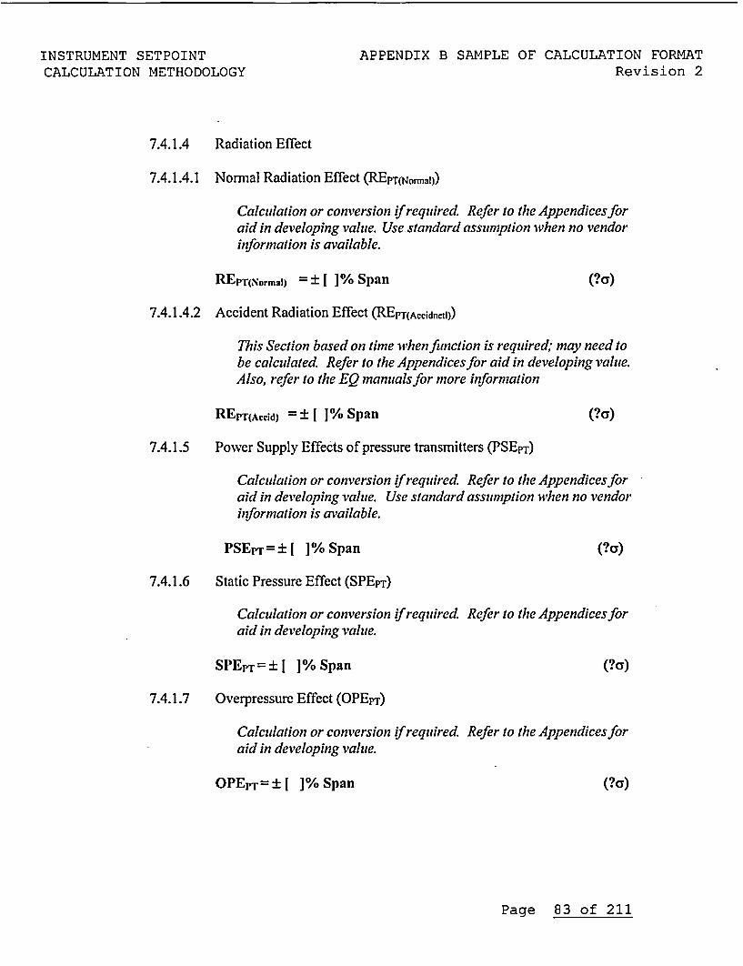
INSTRUMENT SETPOINT APPENDIX B SAMPLE OF CALCULATION FORMATCALCULATION METHODOLOGY Revision 2
7.4.1.4 Radiation Effect
7.4.1.4.1 Normal Radiation Effect (REpT(Norm.a1))
Calculation or conversion ifrequired. Refer to the Appendices foraid in developing value. Use standard assumption when no vendorinformation is available.
REpTvormaI) = ± I ]% Span (?as)
7.4.1.4.2 Accident Radiation Effect (REPT(Accidnetl))
This Section based on time when function is required; may need tobe calculated. Refer to the Appendices for aid in developing value.Also, refer to the EQ manuals for more information
REPT(Accid) = ± I ]% Span (?a)
7.4.1.5 Power Supply Effects of pressure transmitters (PSEPT)
Calculation or conversion ifrequired. Refer to the Appendices foraid in developing value. Use standard assumption when no vendorinformation is available.
PSErr= J[% Span (?a)
7.4.1.6 Static Pressure Effect (SPEpT)
Calculation or conversion ifrequired. Refer to the Appendices foraid in developing value.
SPEPT=±[ ]%Span (?a)
7.4.1.7 Overpressure Effect (OPEpT)
Calculation or conversion ifrequired Refer to the Appendices foraid in developing value.
OPEprT=± % Span (?a)
Page 83 of 211
INSTRUMENT SETPOINT APPENDIX B SAMPLE OF CALCULATION FORMATCALCULATION METHODOLOGY Revision 2
7.4.1.8 Seismic Effect
7.4.1.8.1 Normal Seismic Effect (SEpr(Noma,))
Use standard assunption.
SEPT(Normal) =0
7.4.1.8.2 Accident Seismic Effect (SEpT(Accid))
Per Section C.3.14, A seismic event coincident with a LOCA is adesign basis event per USAR 15.6.5. However, per USAR15.6.5.1.1, there are no realistic, identifiable events which wvouldresult in a pipe break inside the containment of the magnituderequired to cause a loss-of-coolant accident coincident with a safeshutdown earthquake. Therefore, each setpoint calculation shouldconsider the larger effect of a seismic event or loss-of-coolant.
SEPT(Accid) 0 °
7.4.1.8.3 OBE/SSE Seismic Effect (SEpr(scismic))
Refer to the Appendices for aid in developing value. Also, refer tothe SQ manuals for more information
SEprT(seismic) = E I ] % Span (?Ca)
7.4.1.9 RFI/EMI Effect (REEpT)
Use standard assumption, if applicable or review historical workpackages and vendor data to build ajusttfiable assumption.
REEPT= 0
7.4.1.10 Bias (BpT)-
Refer to Appendix Cfor guidance.
BPT = d1 ] % Span (?CY)
7.4.1.11 Pressure Transmitter Accuracy
Refer to Section 7.3.1 forformula.
Page 84 of 211
INSTRUMENT SETPOINT APPENDIX B SAMPLE OF CALCULATION FORMATCALCULATION METHODOLOGY Revision 2
7.4.1.11.1 Normal Pressure Transmitter Accuracy (ApT(Norma1))
ApTNorniaI)= ±1 I% Span (?a)
7.4.1.11.2 Accident Pressure Transmitter Accuracy (ApT(Accid))
Calculated the same as normal, however the accident Uncertaintiesreplace the similar normal uncertainities.
APT(Aceid)= ±1 1% Span (?a)
7.4.1.11.3 Seismic Pressure Transmitter Accuracy (APT(seismic))
Calculated the same as normal, however the seismic uncertaintyreplaces the normal seismic uncertainity.
AT(sas)mi) = ±1 1% Span (?C)
7.4.1.11.4 Pressure Transmitter Accuracy (APT)
Based on the above, use the largest uncertainty is calculated under
[normal/accident/seismic] conditions to determine AV, NTSP, and
CE. Therefore:
APT = ±APT(normal/accident/seismic)
Ar±= ±1% Span (?a)
7.4.2 Loop Accuracy (AL)
Refer to Section 7.3.1 forformula
AL= ±I% Span (2a)
7.5 As-Left Values (ALT)
Each device in loop requires an ALT,.For component,
ALT = (existing ALT or VA) units (3a)
Page 85 of 211
INSTRUMENT SETPOINT APPENDIX B SAMPLE OF CALCULATION FORMATCALCULATION METHODOLOGY Revision 2
The loop As-Left Tolerance (ALT) will be calculated as follows:
Refer to Section 7.3.2forformnla.
ALTL = ±I I units (2a)
7.6 Loop Calibration Error (CL)
Refer to Section 7.3.3forformula
7.6.1 As-Left Tolerance (ALTL)
Refer to Section 7.5for values.
ALTL ±I% Span (2a)
7.6.2 Calibration Tool Error (C;)
Each device requires a calibration tool error.
7.6.2.1 Transmitter Calibration Tool Error (CPT)
Refer to M&TE calculation IP-C-0089, for maximum values however, ifextra margin is required, refer to Appendix Hfor additional guidance.
CpT = ±I ]% Span (3a)
7.6.3 Calibration Standard Error (CSTD):
Per Assumption [ ], Calibration Standard Error is considered negligiblefor the purposes of this analysis.
CSTD =0
7.6.4 Loop Calibration Error (CL):
Calculate usingformulafrom Section 7.6 above. Only the M&TE requiredfor the loop is usedfor calculating the Loop Calibration Error (C).
CL=±I ]%Span (2a)
Page 86 of 211
INSTRUMENT SETPOINT APPENDIX B SAMPLE OF CALCULATION FORMATCALCULATION METHODOLOGY Revision 2
7.7 Loop Drift
Each device requires a dift evaluation.
7.7.1 Pressure Transmitter Drift (DpT):
Calculation or conversion ifrequired. Refer to the Appendices for aidin developing value. Use standard assumption when no vendorinformation is available.
DpTr=I 1% Span (?a)
7.7.2 Loop Drift (DL):
Refer to Section 7.3.4forformula.
DL=±I I% Span (2cy)
7.8 Calculation of As-Found Values (AFT)
Each device in loop requires an AFTl. Refer to Section 7.3.5 forformulas.
For component,
AFTI = ±1 I units (2a)
The loop As-Found Tolerance (AFTL) will be calculated as follows:
AFTL = ±t ] units (2a)
7.9 Process Measurement Accuracy (PMA):
Discussion and calculation as required. Refer to the Appendices foraid in developing value.
PMA=±l ]%Span (?CT)7.10 Primary Element Accuracy (PEA):
Discussion and calculation as required. Refer to the Appendices foraid in developing value.
PEA±= ± I% Span (?CT)
Page 87 of 211
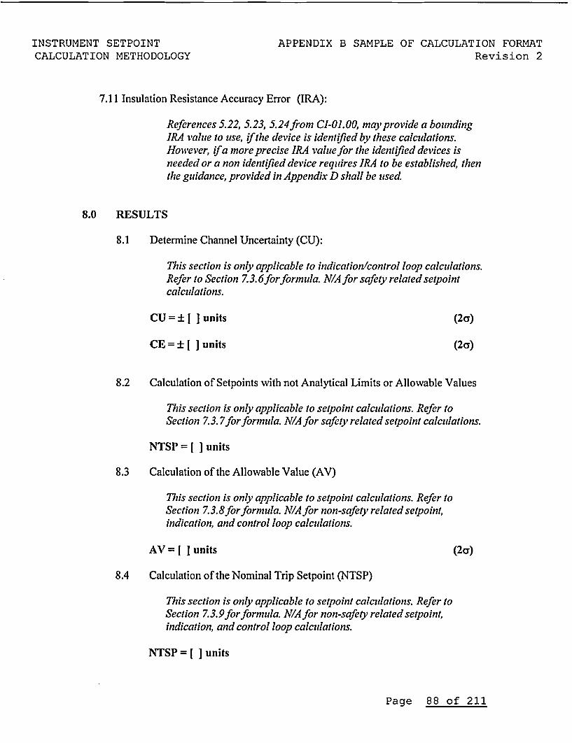
INSTRUMENT SETPOINT APPENDIX B SAMPLE OF CALCULATION FORMATCALCULATION METHODOLOGY Revision 2
7.11 Insulation Resistance Accuracy Error (IRA):
References 5.22, 5.23, 5.24from CI-01.00, may provide a boundingIRA value to use, if the device is identified by these calculations.HowBever, ifa more precise IRA value for the identified devices isneeded or a non identified device requires IRA to be established, thenthe guidance, provided in Appendix D shall be used.
8.0 RESULTS
8.1 Determine Channel Uncertainty (CU):
This section is only applicable to indication/control loop calculations.Refer to Section 7.3. 6 for formula. N/A for safety related setpointcalculations.
CU=[ = units (2a)
CE = ± units (2a)
8.2 Calculation of Setpoints with not Analytical Limits or Allowable Values
This section is only applicable to setpoint calculations. Refer toSection 7.3.7forformula. N/A for safety related setpoint calculations.
NTSP = [ I units
8.3 Calculation of the Allowable Value (AV)
This section is only applicable to setpoint calculations. Refer toSection 7.3.8forformula. N/A for non-safety related setpoint,indication, and control loop calculations.
AV=[ I units (2as)
8.4 Calculation of the Nominal Trip Setpoint (NTSP)
This section is only applicable to setpoint calculations. Refer toSection 7.3.9forformula. N/A for non-safety related setpoint,indication, and control loop calculations.
NTSP = l I units
Page 88 of 211
INSTRUMENT SETPOINTCALCULATION METHODOLOGY
APPENDIX B SAMPLE OF CALCULATION FORMATRevision 2
8.5 Evaluation of Reset Value
Evaluate per guidance given by Section 4.4.12.2
9.0 CONCLUSIONS
Add discussion of results to verbalize that the objectives are met and thatthey graphically presented, the figure should reflect the direction of thesetpoint.
Page 89 of 211
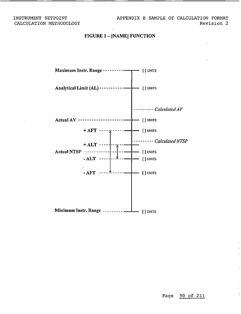
INSTRUMENT SETPOINTCALCULATION METHODOLOGY
APPENDIX B SAMPLE OF CALCULATION FORMATRevision 2
FIGURE 1- [NAME] FUNCTION
Maximum Instr. Range --------- [ I UNITS
Analytical Limit (AL) ---- i------ - - [ ] UNITS
Actual AV ---------------------
+ AFT ------
--------- CalculatedAV
- [I UNITS
-[ ] UNITS
--------- CalculatedNTSP
- [I UNITS
- [I UNITS
- [] UNITS
+ ALT -----
Actual NTSP -----------
- ALT -----
-AFT-
Minimum Instr. Range [ ] UNITS
Page 90 of 211
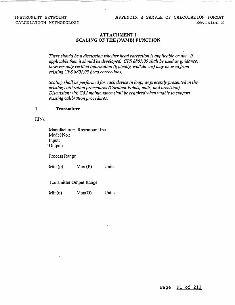
INSTRUMENT SETPOINT APPENDIX B SAMPLE OF CALCULATION FORMATCALCULATION METHODOLOGY Revision 2
ATTACHMENT ISCALING OF THE [NAME) FUNCTION
There should be a discussion whether head correction is applicable or not. Ifapplicable then it should be developed CPS 8801.05 shall be used as guidance,however only verified information (typically, wvalkdowns) may be usedfromexisting CPS 8801.05 head corrections.
Scaling shall be performedfor each device in loop, as presently presented in theexisting calibration procedures (Cardinal Points, units, and precision).Discussion with C&I maintenance shall be required when unable to supportexisting calibration procedures.
1 Transmitter
EINs
Manufacturer: Rosemount Inc.Model No.:Input:Output:
Process Range
Min (p) Max (P) Units
Transmitter Output Range
Min(o) Max(O) Units
Page 91 of 211
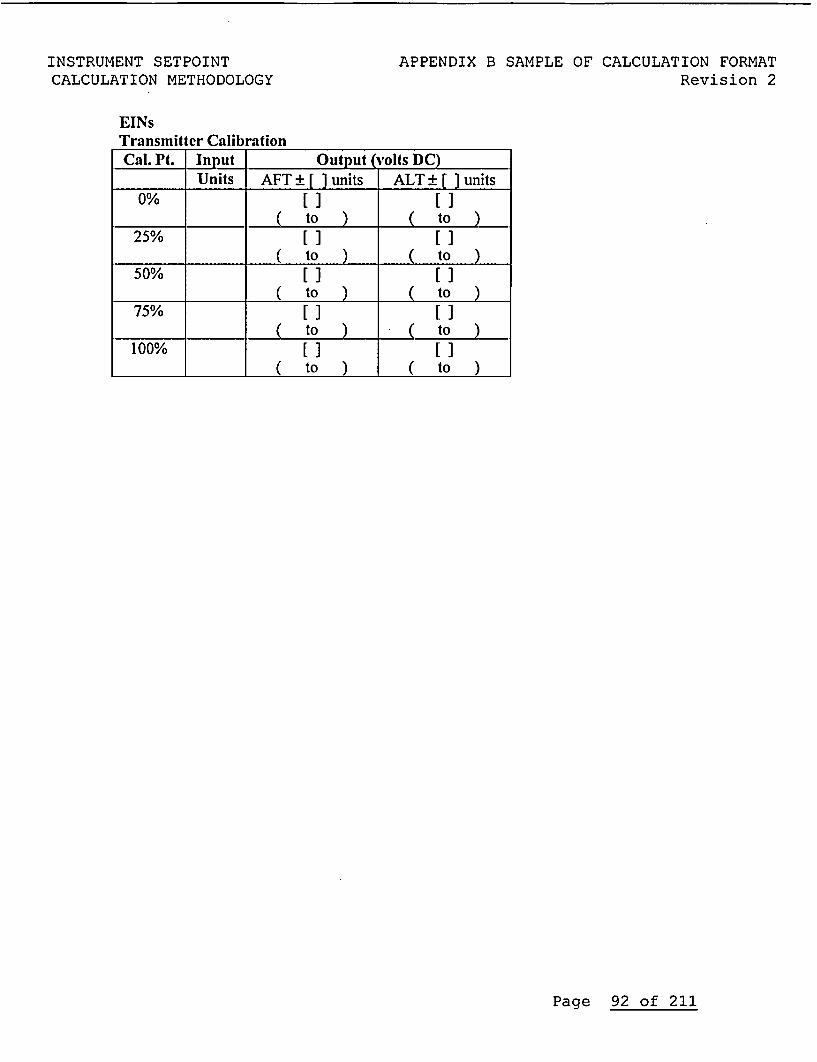
INSTRUMENT SETPOINTCALCULATION METHODOLOGY
APPENDIX B SAMPLE OF CALCULATION FORMATRevision 2
EINsTransmitter CalibrationCal. Pt. Input Output volts DC)
Units AFT+ [ units ALT± [ ] units0% [] []
( to ) ( to )25% [] [ ]
( to ) ( to )50% [] [ ]
( to ) ( to )75% [] [ ]
( to ) ( to )100% [] [ ]
( to ) ( to )
Page 92 of 211
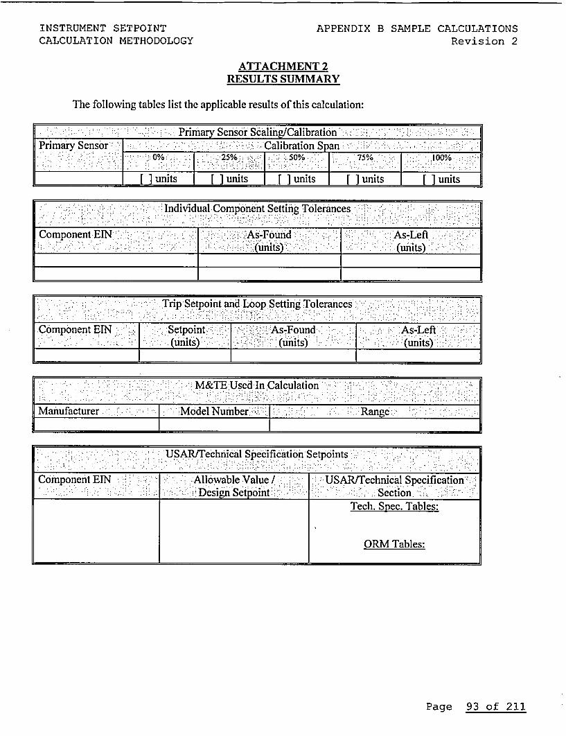
INSTRUMENT SETPOINTCALCULATION METHODOLOGY
APPENDIX B SAMPLE CALCULATIONSRevision 2
ATTACHMENT 2RESULTS SUMMARY
The following tables list the applicable results of this calculation:
Primary Sensor Scaling/CalibrationPrimary Sensor CalibrationSpan
.% 25% ::50% : 75%0 .100%-
[ units [ units [ units [ units [ units
Individual Compo'nentSetting Tolerances
Component-EIN nd ' As-ft
Trip Setpoint and Loop Setting Tolerances'..
.Component EIN .> -Setpoint- As-Found-|--[ uis ' ' units)(u is
:. . M&E Used In'Calculation
Manufacturer J Model Number | .. : Range. ..
USAR/Technical Specification Setpoints
Component EIN -. Allowable Value / -- USAR/Technical Specification%Desig Setpoint Section.:;.
Tech. Spec. Tables:
ORM Tables:
Page 93 of 211
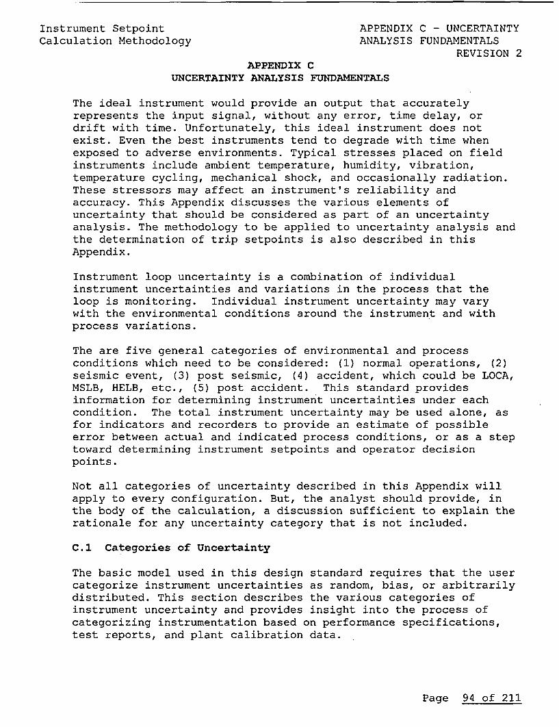
Instrument Setpoint APPENDIX C - UNCERTAINTYCalculation Methodology ANALYSIS FUNDAMENTALS
REVISION 2APPENDIX C
UNCERTAINTY ANALYSIS FUNDAMENTALS
The ideal instrument would provide an output that accuratelyrepresents the input signal, without any error, time delay, ordrift with time. Unfortunately, this ideal instrument does notexist. Even the best instruments tend to degrade with time whenexposed to adverse environments. Typical stresses placed on fieldinstruments include ambient temperature, humidity, vibration,temperature cycling, mechanical shock, and occasionally radiation.These stressors may affect an instrument's reliability andaccuracy. This Appendix discusses the various elements ofuncertainty that should be considered as part of an uncertaintyanalysis. The methodology to be applied to uncertainty analysis andthe determination of trip setpoints is also described in thisAppendix.
Instrument loop uncertainty is a combination of individualinstrument uncertainties and variations in the process that theloop is monitoring. Individual instrument uncertainty may varywith the environmental conditions around the instrument and withprocess variations.
The are five general categories of environmental and processconditions which need to be considered: (1) normal operations, (2)seismic event, (3) post seismic, (4) accident, which could be LOCA,MSLB, HELB, etc., (5) post accident. This standard providesinformation for determining instrument uncertainties under eachcondition. The total instrument uncertainty may be used alone, asfor indicators and recorders to provide an estimate of possibleerror between actual and indicated process conditions, or as a steptoward determining instrument setpoints and operator decisionpoints.
Not all categories of uncertainty described in this Appendix willapply to every configuration. But, the analyst should provide, inthe body of the calculation, a discussion sufficient to explain therationale for any uncertainty category that is not included.
C.1 Categories of Uncertainty
The basic model used in this design standard requires that the usercategorize instrument uncertainties as random, bias, or arbitrarilydistributed. This section describes the various categories ofinstrument uncertainty and provides insight into the process ofcategorizing instrumentation based on performance specifications,test reports, and plant calibration data.
Page 94 of 211
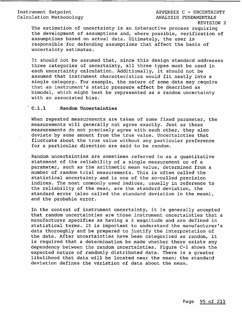
Instrument Setpoint APPENDIX C - UNCERTAINTYCalculation Methodology ANALYSIS FUNDAMENTALS
REVISION 2The estimation of uncertainty is an interactive process requiringthe development of assumptions and, where possible, verification ofassumptions based on actual data. Ultimately, the user isresponsible for defending assumptions that affect the basis ofuncertainty estimates.
It should not be assumed that, since this design standard addressesthree categories of uncertainty, all three types must be used ineach uncertainty calculation. Additionally, it should not beassumed that instrument characteristics would fit neatly into asingle category. For example, the nature of some data may requirethat an instrument's static pressure effect be described asbimodal, which might best be represented as a random uncertaintywith an associated bias.
C.1.1 Random Uncertainties
When repeated measurements are taken of some fixed parameter, themeasurements will generally not agree exactly. Just as thesemeasurements do not precisely agree with each other, they alsodeviate by some amount from the true value. Uncertainties thatfluctuate about the true value without any particular preferencefor a particular direction are said to be random.
Random uncertainties are sometimes referred to as a quantitativestatement of the reliability of a single measurement or of aparameter, such as the arithmetic mean value, determined from anumber of random trial measurements. This is often called thestatistical uncertainty and is one of the so-called precisionindices. The most commonly used indices, usually in reference tothe reliability of the mean, are the standard deviation, thestandard error (also called the standard deviation in the mean),and the probable error.
In the context of instrument uncertainty, it is generally acceptedthat random uncertainties are those instrument uncertainties that amanufacturer specifies as having a ± magnitude and are defined instatistical terms. It is important to understand the manufacturer'sdata thoroughly and be prepared to justify the interpretation ofthe data. After uncertainties have been categorized as random, itis required that a determination be made whether there exists anydependency between the random uncertainties. Figure C-1 shows theexpected nature of randomly distributed data. There is a greaterlikelihood that data will be located near the mean; the standarddeviation defines the variation of data about the mean.
Page 95 of 211
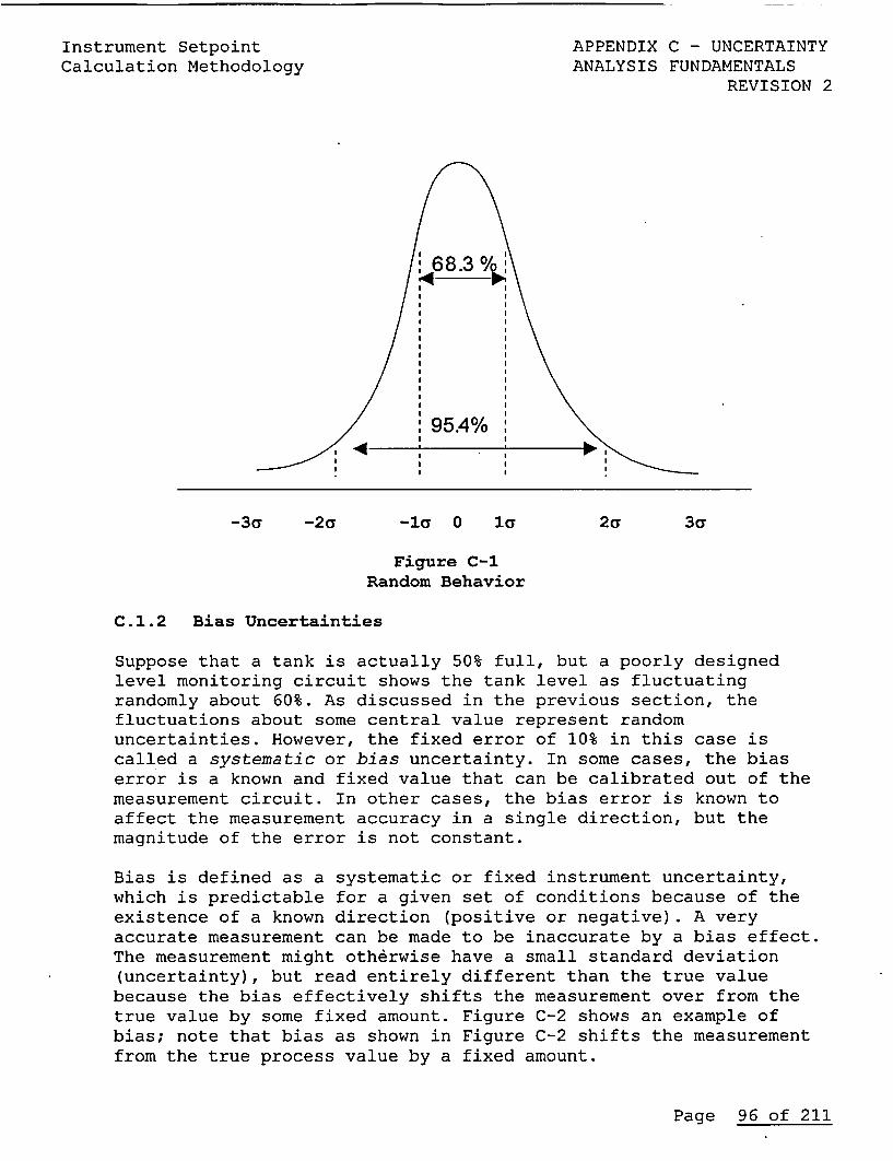
Instrument SetpointCalculation Methodology
APPENDIX C - UNCERTAINTYANALYSIS FUNDAMENTALS
REVISION 2
M.
-35 -2a -is 0 is 2a 3a
Figure C-1Random Behavior
C.1.2 Bias Uncertainties
Suppose that a tank is actually 50% full, but a poorly designedlevel monitoring circuit shows the tank level as fluctuatingrandomly about 60%. As discussed in the previous section, thefluctuations about some central value represent randomuncertainties. However, the fixed error of 10% in this case iscalled a systematic or bias uncertainty. In some cases, the biaserror is a known and fixed value that can be calibrated out of themeasurement circuit. In other cases, the bias error is known toaffect the measurement accuracy in a single direction, but themagnitude of the error is not constant.
Bias is defined as a systematic or fixed instrument uncertainty,which is predictable for a given set of conditions because of theexistence of a known direction (positive or negative). A veryaccurate measurement can be made to be inaccurate by a bias effect.The measurement might otherwise have a small standard deviation(uncertainty), but read entirely different than the true valuebecause the bias effectively shifts the measurement over from thetrue value by some fixed amount. Figure C-2 shows an example ofbias; note that bias as shown in Figure C-2 shifts the measurementfrom the true process value by a fixed amount.
Page 96 of 211
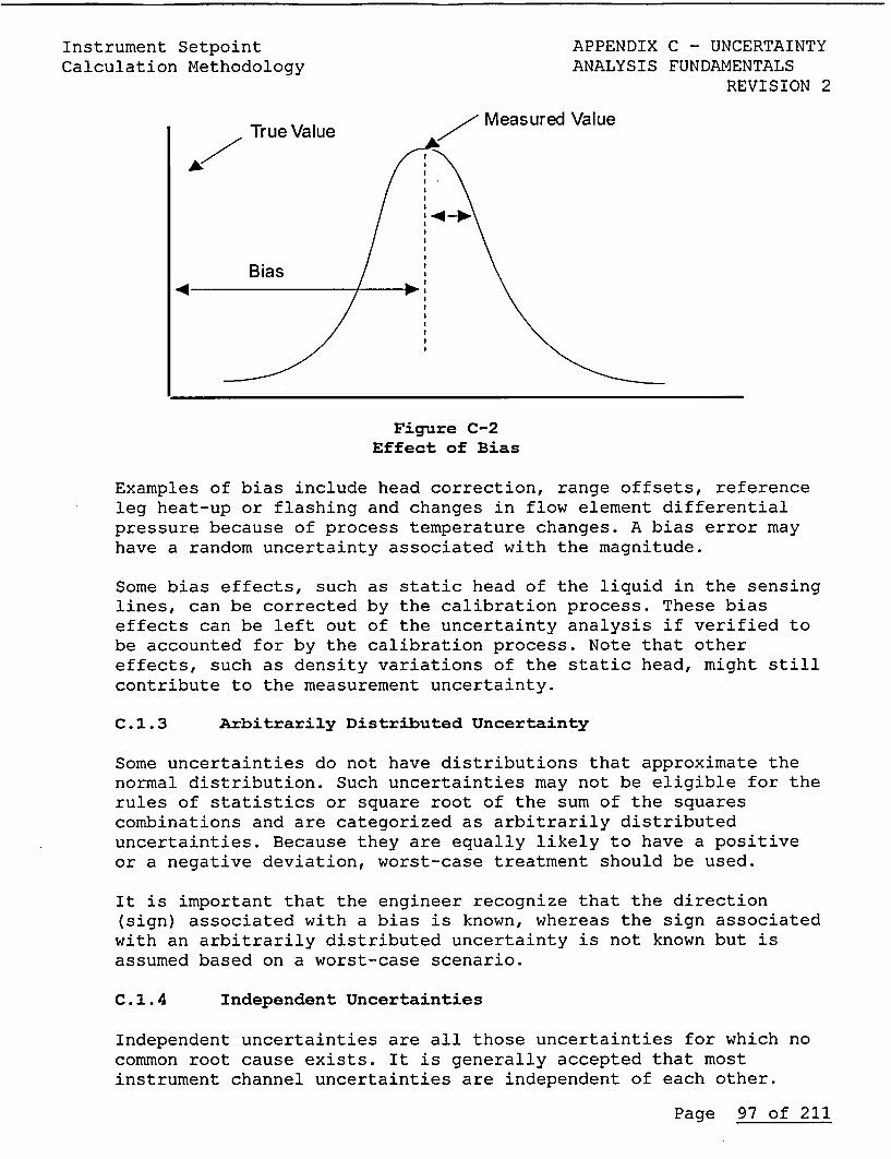
Instrument SetpointCalculation Methodology
APPENDIX C - UNCERTAINTYANALYSIS FUNDAMENTALS
REVISION 2
Measured ValueTrue Value
Bias
Figure C-2Effect of Bias
Examples of bias include head correction, range offsets, referenceleg heat-up or flashing and changes in flow element differentialpressure because of process temperature changes. A bias error mayhave a random uncertainty associated with the magnitude.
Some bias effects, such as static head of the liquid in the sensinglines, can be corrected by the calibration process. These biaseffects can be left out of the uncertainty analysis if verified tobe accounted for by the calibration process. Note that othereffects, such as density variations of the static head, might stillcontribute to the measurement uncertainty.
C.1.3 Arbitrarily Distributed Uncertainty
Some uncertainties do not have distributions that approximate thenormal distribution. Such uncertainties may not be eligible for therules of statistics or square root of the sum of the squarescombinations and are categorized as arbitrarily distributeduncertainties. Because they are equally likely to have a positiveor a negative deviation, worst-case treatment should be used.
It is important that the engineer recognize that the direction(sign) associated with a bias is known, whereas the sign associatedwith an arbitrarily distributed uncertainty is not known but isassumed based on a worst-case scenario.
C.1.4 Independent Uncertainties
Independent uncertainties are all those uncertainties for which nocommon root cause exists. It is generally accepted that mostinstrument channel uncertainties are independent of each other.
Page 97 of 211
Instrument Setpoint APPENDIX C - UNCERTAINTYCalculation Methodology ANALYSIS FUNDAMENTALS
REVISION 2C.1.5 Dependent Uncertainties
Because of the complicated relationships that may exist between theinstrument channels and various instrument uncertainties, it shouldbe recognized that a dependency might exist between someuncertainties. The methodology presented here provides aconservative means for addressing these dependencies. If, in theengineer's judgment, two or more uncertainties are believed to bedependent, then these uncertainties should be added algebraicallyto create a new, larger independent uncertainty. For the purposeof this design standard, dependent uncertainties are those forwhich the user knows or suspects that a common root cause exists,which influences two or more of the uncertainties with a knownrelationship.
C.2 Interpretation of Uncertainty Data
The proper interpretation of uncertainty information is necessaryto ensure that high confidence levels are selected and thatprotective actions are initiated before safety limits are violated.Also, proper interpretation is necessary for the valid comparisonof instrument field performance with setpoint calculationallowances. This comparison confirms the bounding assumptions ofthe appropriate safety analysis.
Accuracy (uncertainty) values should be based on a commonconfidence level (interval) of at least two standard deviations(95% corresponds to approximately 2 standard deviations). The useof three or more standard deviations may be unnecessarilyconservative, resulting in reduced operating margin. Someuncertainty values may need to be adjusted to 2-standard deviationvalues.
For example, if a vendor accuracy for a 99% level (3 standarddeviations) is given as ±6 psig, the 95% confidence levelcorresponds to ±4 psig (= (2/3) x 6). This approach assumes thatvendor data supports this 3 standard deviation claim.
Performance specifications should be provided by instrument orreactor vendors. Data should include vendor accuracy, drift,environmental effects and reference conditions. Since manufacturerperformance specifications often describe a product line, anysingle instrument may perform significantly better than the groupspecification. If performance summary data is not available or ifit does not satisfy the needs of the users, raw test data may needto be reevaluated or created by additional testing.
Page 98 of 211
Instrument Setpoint APPENDIX C - UNCERTAINTYCalculation Methodology ANALYSIS FUNDAMENTALS
REVISION 2If an uncertainty is known to consist of both random and biascomponents, the components should be separated to allow subsequentcombination of like components. Bias components should not be mixedwith random components during the square root of the sum of thesquares combination.
Historically, there have been many different methods ofrepresenting numerical uncertainty. Almost all suffer from theambiguity associated with shorthand notation. For example, withoutfurther explanation, the symbol ± is often interpreted as thesymmetric confidence interval associated with a random, normallydistributed uncertainty. Further, the level of confidence may beassumed to be 68% (standard error, 1 standard deviation), 95% (2standard deviations) or 99% (3 standard deviations). Still othersmay assume that the ± symbol defines the limits of error(reasonable bounds) of bias or non-normally distributeduncertainties. Vendors should be consulted to avoid anymisinterpretation of their performance specifications or testresults.
Reactor vendors typically utilize nominal values for uncertaintiesused in a setpoint analysis associated with initial plantoperation. These generic values are considered conservativeestimates, which may be refined if plant-specific data isavailable. Since plant-specific data may be less conservative thanthe bounding generic data, care should be taken to ensure that itis based on a statistically significant sample size.
One source of performance data that requires careful interpretationis that obtained during harsh environment testing. Often, suchtests are conducted only to demonstrate the functional capabilityof a particular instrument in a harsh environment. This usuallyrequires only a small sample size and invokes inappropriaterejection criteria for a probabilistic determination of instrumentuncertainties. The meager data base typically results in limits oferror (reasonable bounds) associated with bias or non-normallydistributed uncertainties.
The limited database from an environmental qualification test alsoprecludes adjusting the measured net effects for normalenvironmental uncertainties, vendor accuracies, etc. Thus, theresults of such tests describe several mutually exclusivecategories of uncertainty. For example, the results of a severeenvironment test may contain uncertainty contributions from theinstrument vendor accuracy, measuring and test equipmentuncertainty, calibration uncertainty and others, in addition to thesevere environment effects. A conservative practice is to treat themeasured net effects as only uncertainty contributions due to theharsh environment.
Page 99 of 211
Instrument Setpoint APPENDIX C - UNCERTAINTYCalculation Methodology ANALYSIS FUNDAMENTALS
REVISION 2In summary, avoid improper use of vendor performance data. Just asimportant, do not apply overly conservative values to uncertaintyeffects to the point that a setpoint potentially limits normaloperation or expected operational transients. Because of thediversity of data summary techniques, notational ambiguities,inconsistent terminology and ill-defined concepts that have beenapparent in the past, it is recommended that vendors be consultedwhenever questions arise. If a vendor-published value of anuncertainty term (source) is confirmed to contain a significantbias uncertainty, then the ± value should be treated as anestimated limit of error. If the term is verified to represent onlyrandom uncertainties (no significant bias uncertainties), then the+ value should be treated as the 2-standard deviation interval foran approximately normally distributed random uncertainty.
C.3 Elements of Uncertainty
NOTE: The following sections may expand or add clarification forelements of uncertainty, but does not replace the definitionsspecified in Section 2.2.
C.3.1 Process Measurement Accuracy (PMA)
PMA are those effects that have a direct effect on the accuracy ofa measurement. PMA variables are independent of the processinstrumentation used to measure the process parameter. PMA canoften be thought of as physical changes in the monitored parameterthat cannot be detected by conventional instrumentation.
The following are examples of PMA variables:
* Temperature stratification and inadequate mixing of bulktemperature measurements
* Reference leg heatup and process fluid density changes fromcalibrated conditions
* Piping configuration effects on level and flow measurements* Fluid density effects on flow and level measurements* Line pressure loss and pressure head effects
* Temperature variation effect on hydrogen partial pressure* Gas density changes on radiation monitoring
Some PMA terms are easily calculated, some PMA terms are quitecomplex and are obtained from General Electric documents, and otherPMA terms are allowances developed and justified by Design BasisDocuments.
Page 100 of 211

Instrument SetpointCalculation Methodology
APPENDIX C - UNCERTAINTYANALYSIS FUNDAMENTALS
REVISION 2C.3.2 Primary Element Accuracy (PEA)
PEA is generally described as the accuracy associated with theprimary element, typically a flow measurement device such as anorifice, venturi, or other devices from which a process measurementsignal is developed. The following devices are typically consideredto have a primary element accuracy that requires evaluation in anuncertainty analysis:
* Flow venturi6
6
6
6
Flow nozzleOrifice plateRTD or thermocouple thermowellSealed sensors such as a bellows unit to transmit a pressuresignal
PEA can change over time because of erosion, corrosion, ordegradation of the sensing device. Installation uncertainty effectscan also contribute to PEA errors.
Page 101 of 211
---- C
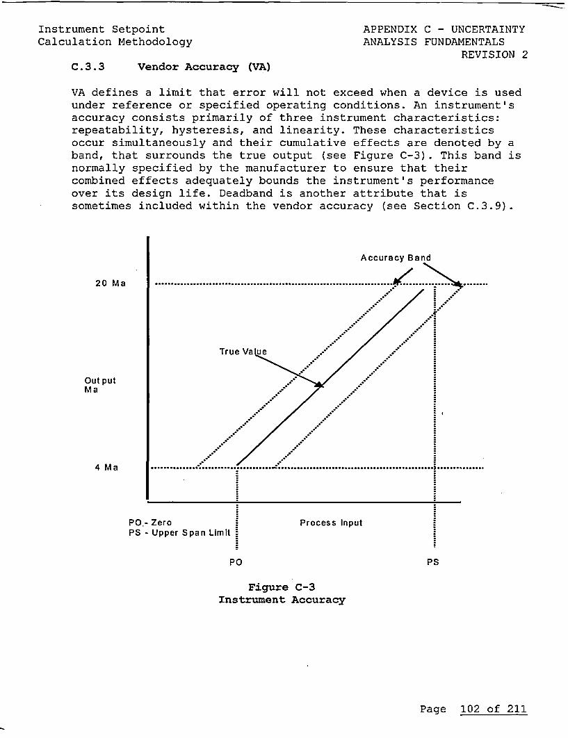
Instrument Setpoint APPENDIX C - UNCERTAINTYCalculation Methodology ANALYSIS FUNDAMENTALS
REVISION 2C.3.3 Vendor Accuracy (VA)
VA defines a limit that error will not exceed when a device is usedunder reference or specified operating conditions. An instrument'saccuracy consists primarily of three instrument characteristics:repeatability, hysteresis, and linearity. These characteristicsoccur simultaneously and their cumulative effects are denoted by aband, that surrounds the true output (see Figure C-3). This band isnormally specified by the manufacturer to ensure that theircombined effects adequately bounds the instrument's performanceover its design life. Deadband is another attribute that issometimes included within the vendor accuracy (see Section C.3.9).
Accuracy Band
20 Ma ........................................................................... .............. ........
True Va ue
Out putMa
4Ma . ..
PO.- Zero Process InputPS - Upper Span Limit
PO PS
Figure C-3Instrument Accuracy
Page 102 of 211
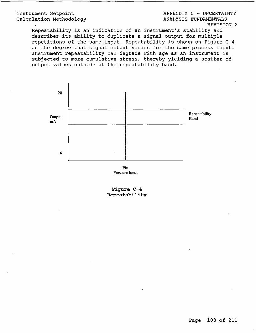
InstiCalcL
-ument Setpoint APPENDIX C - UNCERTAINTYilation Methodology ANALYSIS FUNDAMENTALS
REVISION 2Repeatability is an indication of an instrument's stability anddescribes its ability to duplicate a signal output for multiplerepetitions of the same input. Repeatability is shown on Figure C-4as the degree that signal output varies for the same process input.Instrument repeatability can degrade with age as an instrument issubjected to more cumulative stress, thereby yielding a scatter ofoutput values outside of the repeatability band.
20
OutputmA
4
1*
RepeatabilityBand
PinPressure Input
Figure C-4Repeatability
Page 103 of 211
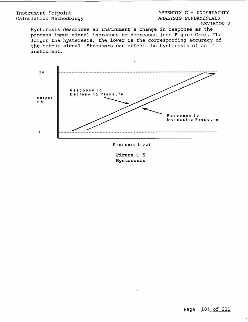
Instrument SetpointCalculation Methodology
APPENDIX C - UNCERTAINTYANALYSIS FUNDAMENTALS
REVISION 2Hysteresis describes an instrument's change in response as theprocess input signal increases or decreases (see Figure C-5). Thelarger the hysteresis, the lower is the corresponding accuracy ofthe output signal. Stressors can affect the hysteresis of aninstrument.
2 0 .....................................................................................................
Response toDecreasing Pressure
Out put /rnA
Res po n se toIncreasing Pressure
4 .....................................................................................................
Pressure Input
Figure C-5Hysteresis
Page 104 of 211
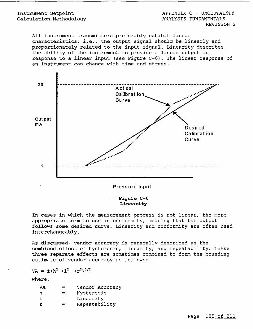
Instrument Setpoint APPENDIX C - UNCERTAINTYCalculation Methodology ANALYSIS FUNDAMENTALS
REVISION 2
All instrument transmitters preferably exhibit linearcharacteristics, i.e., the output signal should be linearly andproportionately related to the input signal. Linearity describesthe ability of the instrument to provide a linear output inresponse to a linear input (see Figure C-6). The linear response ofan instrument can change with time and stress.
2 0 ................................................................................................ .A ct u a l .
Ca librat ion .. ;:;Curve A
Out putmA mA/ Desired
/. Ca librat ion/ ~Cu.rve
4 ................. .................... ... .... .... .... ... .... ... .
Pressure Input
Figure C-6Linearity
In cases in which the measurement process is not linear, the moreappropriate term to use is conformity, meaning that the outputfollows some desired curve. Linearity and conformity are often usedinterchangeably.
As discussed, vendor accuracy is generally described as thecombined effect of hysteresis, linearity, and repeatability. Thesethree separate effects are sometimes combined to form the boundingestimate of vendor accuracy as follows:
VA = ±(h2 +12 +r2) 1/2
where,
VA Vendor Accuracyh Hysteresis1 = Linearityr = Repeatability
Page 105 of 211
Instrument Setpoint APPENDIX C - UNCERTAINTYCalculation Methodology ANALYSIS FUNDAMENTALS
REVISION 2
Accuracy cannot be adjusted, improved, or otherwise affected by thecalibration process. Rather, accuracy is a performancespecification against which the device is tested during calibrationto determine its condition. A 5-point calibration check, (0%, 25%,50%, 75%, and 100%), of an instrument's entire span verifieslinearity. If a 9-point check is performed, by checking up to 100%and back down to 0%, hysteresis is also verified. Finally, if thecalibration check is performed a second time (or more),repeatability is verified. The calibration check process is rarelyperformed to a level of detail that also confirms repeatability butif it is, per ISA S 67.04, both vendor accuracy and thecalibrations tolerance do not both need to be included in theuncertainty analysis. For this reason, the vendor accuracy termshould be checked to verify that it includes the combined effectsof linearity, hysteresis, and repeatability. If the vendor accuracyspecification does not include all of these terms, the missingterms are included into the vendor accuracy specification asfollows:
VA = ±(va2 + h2 +12 +r2) 1/2
where,
VA Revised estimate of vendor accuracyva = Vendor's stated accuracy with some terms not includedh = Hysteresis (if not already included)1 = Linearity (if not already included)r = Repeatability (if not already included)
Vendor accuracy is considered an independent and random uncertaintycomponent unless the manufacturer specifically states that a biasor dependent effect also exists. Vendor accuracy is normallyexpressed as a percent of instrument span, but this should beconfirmed from the manufacturer's specifications.
Bistables, trip units, and pressure switches may not require aconsideration of hysteresis and linearity because the calibrationmight be checked only at the setpoint. If the accuracy is checkedat the setpoint for these devices, the accuracy elsewhere in theinstrument's span is not directly verified.
The calibration process might not adequately confirm the vendoraccuracy if the measuring and test equipment (M&TE) uncertaintysignificantly exceeds the accuracy of the device being calibrated.For example, the calibration process cannot verify a 0.1% accuracyspecification with M&TE having an uncertainty of 0.5%. If the M&TEuncertainty exceeds the specified vendor accuracy, then the vendoraccuracy should be considered no better than the M&TE allowance.
Page 106 of 211
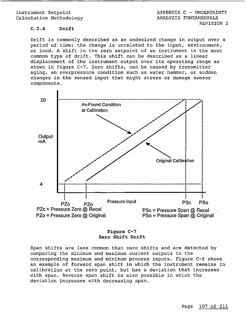
Instrument Setpoint APPENDIX C - UNCERTAINTYCalculation Methodology ANALYSIS FUNDAMENTALS
REVISION 2C.3.4 Drift
Drift is commonly described as an undesired change in output over aperiod of time; the change is unrelated to the input, environment,or load. A shift in the zero setpoint of an instrument is the mostcommon type of drift. This shift can be described as a lineardisplacement of the instrument output over its operating range asshown in Figure C-7. Zero shifts, can be caused by transmitteraging, an overpressure condition such as water hammer, or suddenchanges in the sensed input that might stress or damage sensorcomponents.
20.-.As-Found Conditionat Calibration
Output 0*MA
Pc Po Pressure Input PSC PSoPZc = Pressure Zero @ Recal PSc = Pressure Span @ RecalPZo = Pressure Zero @ Original PSo = Pressure Span @ Original
Figure C-7Zero Shift Drift
Span shifts are less common than zero shifts and are detected bycomparing the minimum and maximum current outputs to thecorresponding maximum and minimum process inputs. Figure C-B showsan example of forward span shift in which the instrument remains incalibration at the zero point, but has a deviation that increaseswith span. Reverse span shift is also possible in which thedeviation increases with decreasing span.
Page 107 of 211
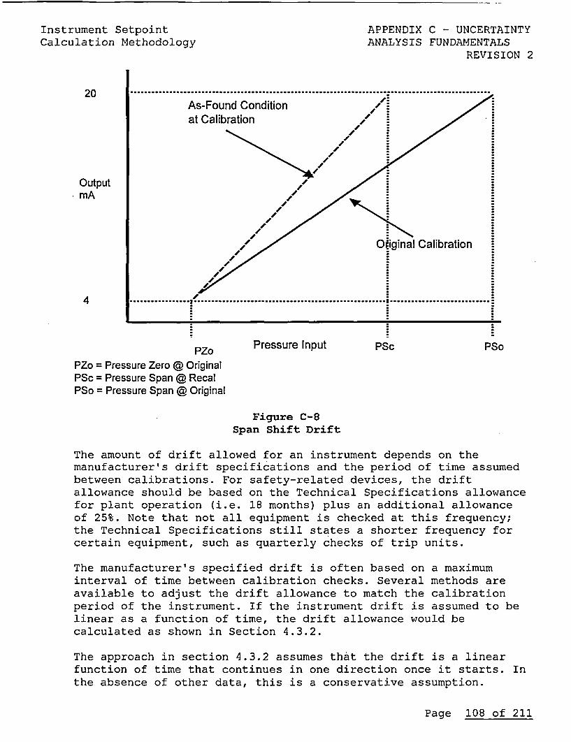
Instrument Setpoint APPENDIX C - UNCERTAINTYCalculation Methodology ANALYSIS FUNDAMENTALS
REVISION 2
2 0 ........................................................................ .................................................
As-Found Conditionat Calibration
Output*mA
41
,' /Original Calibration
4 ................. ............................... ...............
PZO Pressure Input PSc PSo
PZo = Pressure Zero © OriginalPSc = Pressure Span @ RecalPSo = Pressure Span @ Original
Figure C-8Span Shift Drift
The amount of drift allowed for an instrument depends on themanufacturer's drift specifications and the period of time assumedbetween calibrations. For safety-related devices, the driftallowance should be based on the Technical Specifications allowancefor plant operation (i.e. 18 months) plus an additional allowanceof 25%. Note that not all equipment is checked at this frequency;the Technical Specifications still states a shorter frequency forcertain equipment, such as quarterly checks of trip units.
The manufacturer's specified drift is often based on a maximuminterval of time between calibration checks. Several methods areavailable to adjust the drift allowance to match the calibrationperiod of the instrument. If the instrument drift is assumed to belinear as a function of time, the drift allowance would becalculated as shown in Section 4.3.2.
The approach in section 4.3.2 assumes that the drift is a linearfunction of time that continues in one direction once it starts. Inthe absence of other data, this is a conservative assumption.
Page 108 of 211
Instrument Setpoint APPENDIX C - UNCERTAINTYCalculation Methodology ANALYSIS FUNDAMENTALS
REVISION 2However, if the vendor states that the drift during the calibrationperiod is random and independent, then it is just as likely fordrift to randomly change directions during the calibration period.In this case, the square root of the sum of the squares of theindividual drift periods between calibrations could be used. Inthis case, the total drift allowance for 30 months would be:
DR30 ±(0. 5%2 + 0.5%2 + 0Q5%2 + 0.5%2 + Q.5%2) /2 = ±1.12% of span
Some vendors have stated that the majority of drift tends to occurin the first several months following a calibration and that theinstrument output will not drift significantly after the "settle-inperiod." In this case, a lower drift value might be acceptableprovided that the vendor can supply supporting data of this type ofdrift characteristic. However, when the vendor stated drift is fora longer period (i.e. Rosemount drift = 0.2% for 30 months) thenthe calibration period it is not acceptable to arbitrarily reducethe drift value. In this case the data supporting a "settle-inperiod" drift characteristic must be evaluated.
VD3 0 =[VDyr2 + VDyr 2 + (VDyr 2 * 2)] 1/2
In the above expression of drift, VDyr represents the annual driftestimate and the resultant drift, VD3 0, represents the 30-monthdrift estimate. If VDyr = 1%, the 30-month drift estimate isobtained by:
VD30 = ±[1.0%2 + 1.0%2 + (1.0%2 - 2)] 1/2= +1.58% of span
Drift can also be inferred from instrument calibration data by ananalysis of as-found and as-left data. Typically, the variationbetween the as-found reading obtained during the latest calibrationand the as-left reading from the previous calibration is taken tobe indicative of the drift during the calibration interval. Byevaluating the drift over a number of calibrations for functionallyequivalent instruments, an estimate of the drift can be developed.Typically, the calibration data is used to calculate the mean ofdrift, the standard deviation of drift, and the tolerance intervalthat contains a defined portion of the drift data to a certainprobability and confidence level (typically 95%/95%). Thisstatistically determined value of drift can be used to validate thevendor's performance specification and can also be used as the bestestimate of drift in the uncertainty calculation. Assigning all ofthe statistically determined drift from plant specific data isespecially conservative because this drift allowance contains manyother contributors to uncertainty, including:
Instrument hysteresis and linearity error present during thefirst calibration
Page 109 of 211
Instrument Setpoint APPENDIX C - UNCERTAINTYCalculation Methodology ANALYSIS FUNDAMENTALS
REVISION 2
* Instrument hysteresis and linearity error present during thesecond calibration
* Instrument repeatability error present during the firstcalibration
* Instrument repeatability error present during the secondcalibration
* Measurement and test equipment error present during the firstcalibration
* Measurement and test equipment error present during the secondcalibration
* Personnel-induced or human-related variation or error duringthe first calibration
* Personnel-induced or human-related variation or error duringthe second calibration
* Instrument temperature effects due to a difference in ambienttemperature between the two calibrations (this is particularlytrue for 18 month cycle plants in which the first calibrationis performed in the winter and the second calibration isperformed in the summer)
* Environmental effects on instrument performance, e.g.,radiation, temperature, vibration, etc., between the twocalibrations that cause a shift in instrument output
* Misapplication, improper installation, or other operatingeffects that affect instrument calibration during the periodbetween calibrations
* True instrument "drift" representing a change, time-dependentor otherwise, in instrument output over the time periodbetween calibrations
Regardless of the approach taken for determining the driftallowance, the uncertainty calculation should provide the basis forthe value used.
C.3.5 Accuracy Temperature Effects (ATE)
The ambient temperature is expected to vary somewhat during normaloperation. This expected temperature variation can influence aninstrument's output signal and the magnitude of the effect isreferred to as the temperature effect. Using a maximum temperaturethat bounds the maximum observed temperature can reduce theconservatism of using the maximum temperature difference. Largertemperature changes associated with accident conditions areconsidered part of the environmental allowance and the effect oflarger temperature changes was determined as part of anenvironmental qualification test. The temperature effects describedhere only relate to the effect on instrument performance duringnormal operation.
Page 110 of 211
Instrument Setpoint APPENDIX C - UNCERTAINTYCalculation Methodology ANALYSIS FUNDAMENTALS
REVISION 2The vendor normally provides an allowance for the predicted effecton instrument performance as a function of temperature. Forexample, a typical temperature effect might be ±0.75% per 1000 Fchange from the calibrated temperature. This vendor statement ofthe temperature effect would be correlated to plant-specificperformance as follows:
ATE = ±(Int - ctl) (vte)
where,
ATE = Temperature effect to assume for the uncertaintycalculation
nt = Normal expected maximum or minimum temperature (bothsides should be checked)
ct = Calibration temperature (typically, minimum zone temp.)vte = Vendor's temperature effects expression
For example, if the vendor's temperature effects expression is±0.75% of span per 1000F, the calibration temperature is 650F ifknown, otherwise use the minimal temperature for that zone, and themaximum expected temperature is 110'F. This vendor statement of thetemperature effect would be correlated to plant-specificperformance as follows:
ATE = ±[j 1100 F - 65OF1 x (0.75% . 1000F)] = ± 0.3375% of span
Notice that the above approach starts with the minimal zonetemperature, and then determines the maximum expected variationfrom the minimal zone temperature under normal operatingconditions. Design Criteria DC-ME-09-CP "Equipment EnvironmentalDesign Conditions" provides all normal and harsh environments forthe plant.
The above discussion applies to temperature effects oninstrumentation, in response to expected ambient temperaturevariations during normal plant operation. Some manufacturers havealso identified accident temperature effects that describe theexpected temperature effect on instrumentation for even largerambient temperature variations. An accident temperature effectdescribes an uncertainty limit for instrumentation operatingoutside the normal environmental limits and in some cases mayinclude normal temperature effects.
Temperature effect is considered a random error term unlessotherwise specified by the manufacturer.
Page 111 of 211
Instrument Setpoint APPENDIX C - UNCERTAINTYCalculation Methodology ANALYSIS FUNDAMENTALS
REVISION 2C.3.6 Radiation Effects (RE)
During normal operation, most plant equipment is exposed torelatively low radiation levels. Although the lower dose rate,.radiation effects, might have a nonreversible effect on aninstrument, the calibration process can eliminate them. If the doserate is low enough, the ambient environment might be consideredmild during normal operation and radiation effects can beconsidered negligible. Any effects of relatively low radiationeffects are considered indistinguishable from drift and arecalibrated out during routine calibration checks.
If the normal operation dose rate is high enough that radiationeffects should be considered, the environmental qualification testreport will provide the best source of radiation effectinformation. During the worst-case accident environment, radiationeffects can be part of the simultaneous effect of temperature,pressure, steam, and radiation that was determined during theenvironmental qualification process. Other plant locations mightexperience a more benign temperature and pressure environment, butstill be exposed to significant accident radiation. For each case,the determination of the radiation effects should rely on the datain the environmental qualification report. Environmentalqualification test report data should usually be treated as anarbitrarily distributed bias unless the manufacturer has provideddata supporting its treatment as a random contributor touncertainty.
C.3.7 Static Pressure Effects (SPE)
Some devices exhibit a change in output because of changes inprocess or ambient pressure. A differential pressure transmittermight measure flow across an orifice with a differential pressureof a few hundred inches of water while the system pressure is over1,000 psig. The system pressure is essentially a static pressureplaced on the differential pressure measurement. The vendor usuallyspecifies the static pressure effect; a typical example is shownbelow:
Static pressure effect = ±0.5% of span per 1,000 psig
The static pressure effect is a consequence of calibrating adifferential pressure instrument at low static pressure conditions,but operating at high static pressure conditions.
Page 112 of 211
Instrument Setpoint APPENDIX C - UNCERTAINTYCalculation Methodology ANALYSIS FUNDAMENTALS
REVISION 2If the static pressure effect is considered a bias by themanufacturer, the operating manual usually provides instructionsfor calibrating the instrument to read correctly at the normalexpected operating pressure, assuming that the calibration isperformed at low static pressure conditions. This normally involveschanging the zero and span adjustments by a manufacturer-suppliedcorrection factor at the low-pressure (calibration) conditions sothat the instrument will provide the desired output signal at thehigh-pressure (operating) conditions. The device could also becalibrated at the expected operating pressure to reduce oreliminate this effect, but is not normally done because of thehigher calibration cost and complexity.
Some static pressure effects act as a bias rather than randomly.For example, some instruments are known to read low at high staticpressure conditions. If the calibration process does not correctthe bias static pressure effect, the uncertainty calculation needsto include a bias term to account for this effect.
Ambient pressure variation can cause some gauge and absolutepressure instruments to shift up or down scale depending on whetherthe ambient pressure increases above or decreases below atmosphericpressure. Normally, this effect is only significant on 1)applications measuring very small pressures or 2) applications inwhich the ambient pressure variations are significant with respectto the pressure being measured. Gauge pressure instruments can besensitive to this effect when the reference side of a sensingelement is open to the atmosphere. If the direction of the ambientpressure change is known, the effect is a bias. If the ambientpressure can randomly change in either direction, the effect isconsidered random.
C.3.8 Overpressure Effect (OPE)
In cases where an instrument can be over-ranged by the processpressure without the process pressure exceeding system designpressure, an overpressure effect must be considered. Overpressureeffects are often considered in low-range monitoring instruments inwhich the reading is expected to go off-scale high as the systemshifts from shutdown to operating conditions. Some pressureswitches may also be routinely over-ranged during normal operation.The overpressure effect is normally considered random and isusually expressed as a percent uncertainty as a function of theamount of overpressure. The contribution of the overpressure effecton instrument uncertainty would only apply after the instrument hasbeen over-ranged.
Page 113 of 211
Instrument Setpoint APPENDIX C - UNCERTAINTYCalculation Methodology ANALYSIS FUNDAMENTALS
REVISION 2C.3.9 Deadband
Deadband represents the range within which the input signal canvary without experiencing a change'in the output. The idealinstrument would have no deadband and would respond to inputchanges regardless of their magnitude. Instrument stressors canchange the deadband width over time, effectively requiring agreater change in the input before an output response is achieved.
The vendor's instrument accuracy specification might include anallowance for deadband or it might be considered part of hysteresis(included in vendor accuracy). Recorders generally have a separateallowance for deadband to account for the amount the input signalcan change before the pen physically responds to change.
Pressure switches are also susceptible to deadband. For thisreason, a pressure switch setpoint near the upper or lower end ofspan should confirm that the setpoint allows for deadband. Inextreme cases, the pressure switch might reach a mechanical stopwith the deadband not allowing switch actuation.
C.3.10 Measuring and Test Equipment Uncertainty
Measuring and test equipment (M&TE) uncertainty is defined inSection 2.2 and further described in Appendix H.
C.3.11 Turndown Ratio Effect
If a transmitter has an adjustable span over some total range, theuncertainty expression may require adjustment by the turndownfactor. For example, a transmitter may have a range of 3,000 psigwith an uncertainty of 2% of the total range, sometimes referred toas the upper range limit (URL). If the span is adjusted such thatonly 1,000 psig of the entire 3,000 psig range is used, thetransmitter has not somehow become more accurate. The 2%uncertainty of the 3,000 psig span is 60 psig, which equates to a6% uncertainty for the 1,000 psig span. Transmitters with variablespans typically define performance specifications in terms of thetotal range and the calibrated span.
If the performance specifications are quoted as a percent of fullspan (FS), the uncertainty expression will not require anadjustment for the turndown factor.
Page 114 of 211
Instrument Setpoint APPENDIX C - UNCERTAINTYCalculation Methodology ANALYSIS FUNDAMENTALS
REVISION 2C.3.12 Power Supply Effects (PSE)
Power supply effects are the changes in an instrument's input-output relationship due to the power supply stability. For 2-wirecurrent loop systems, AC supply variations must be considered fortheir effects on the loop's DC power supply. The consequential DCsupply variations must then be considered for their effects onother components in the series loop, such as the transmitter.
Using the manufacturer's specifications, the power supply istypically calculated as follows:
PSE = (pss) (vpse)
where,
PSE = Power supply effect to assume for the uncertainty calculationpss = Power supply stabilityvpse = Vendor's power supply effect expression
Power supply stability refers to the variation in the power supplyvoltage under design conditions of supply voltage, ambientenvironment conditions, power supply accuracy, regulation, anddrift. This effect can be neglected when it can be shown that theerror introduced by power supply variation is <10% of theinstrument's reference accuracy.
Harmonic distortion on the electrical system can also contribute topower supply uncertainty.
Page 115 of 211
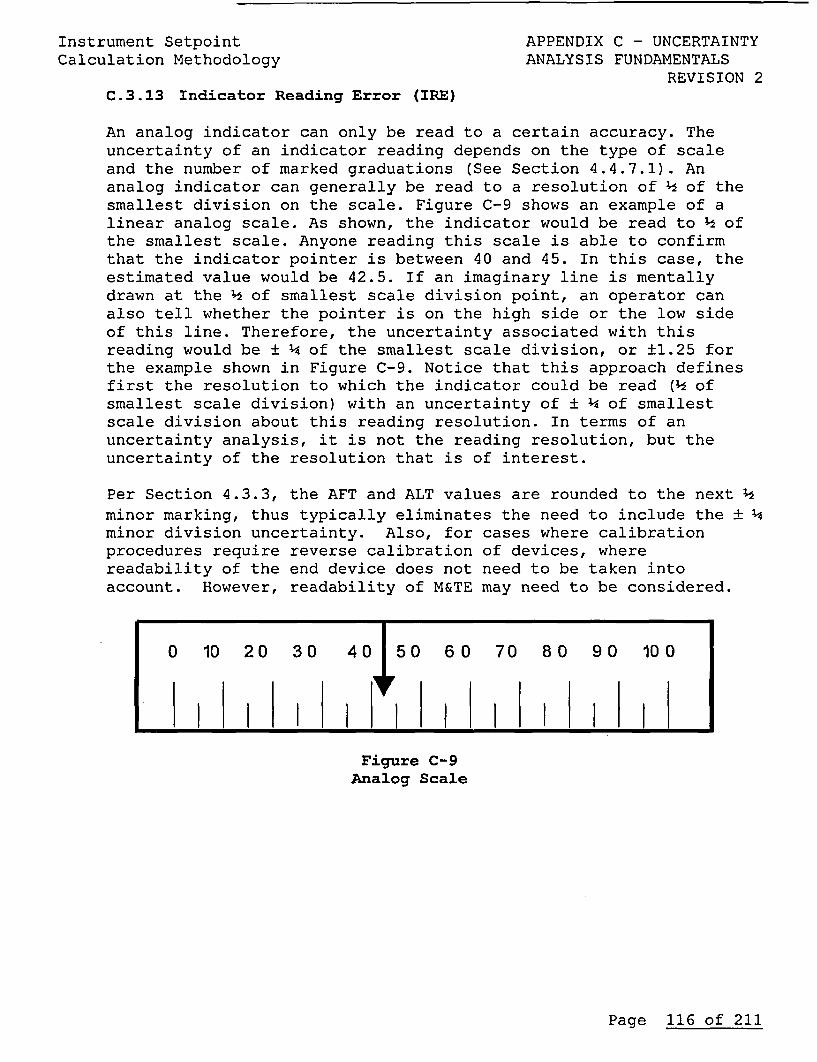
Instrument Setpoint APPENDIX C - UNCERTAINTYCalculation Methodology ANALYSIS FUNDAMENTALS
REVISION 2C.3.13 Indicator Reading Error (IRE)
An analog indicator can only be read to a certain accuracy. Theuncertainty of an indicator reading depends on the type of scaleand the number of marked graduations (See Section 4.4.7.1). Ananalog indicator can generally be read to a resolution of - of thesmallest division on the scale. Figure C-9 shows an example of alinear analog scale. As shown, the indicator would be read to k ofthe smallest scale. Anyone reading this scale is able to confirmthat the indicator pointer is between 40 and 45. In this case, theestimated value would be 42.5. If an imaginary line is mentallydrawn at the i of smallest scale division point, an operator canalso tell whether the pointer is on the high side or the low sideof this line. Therefore, the uncertainty associated with thisreading would be ± :4 of the smallest scale division, or ±1.25 forthe example shown in Figure C-9. Notice that this approach definesfirst the resolution to which the indicator could be read (d ofsmallest scale division) with an uncertainty of ± "i of smallestscale division about this reading resolution. In terms of anuncertainty analysis, it is not the reading resolution, but theuncertainty of the resolution that is of interest.
Per Section 4.3.3, the AFT and ALT values are rounded to the next k
minor marking, thus typically eliminates the need to include the i k
minor division uncertainty. Also, for cases where calibrationprocedures require reverse calibration of devices, wherereadability of the end device does not need to be taken intoaccount. However, readability of M&TE may need to be considered.
0 10 20 3 0 4 0 50 6 0 70 8 0 9 0 10 0
.I I I I I I *I I I I 1 1 1 1 , 1 IFigure C-9
Analog Scale
Page 116 of 211
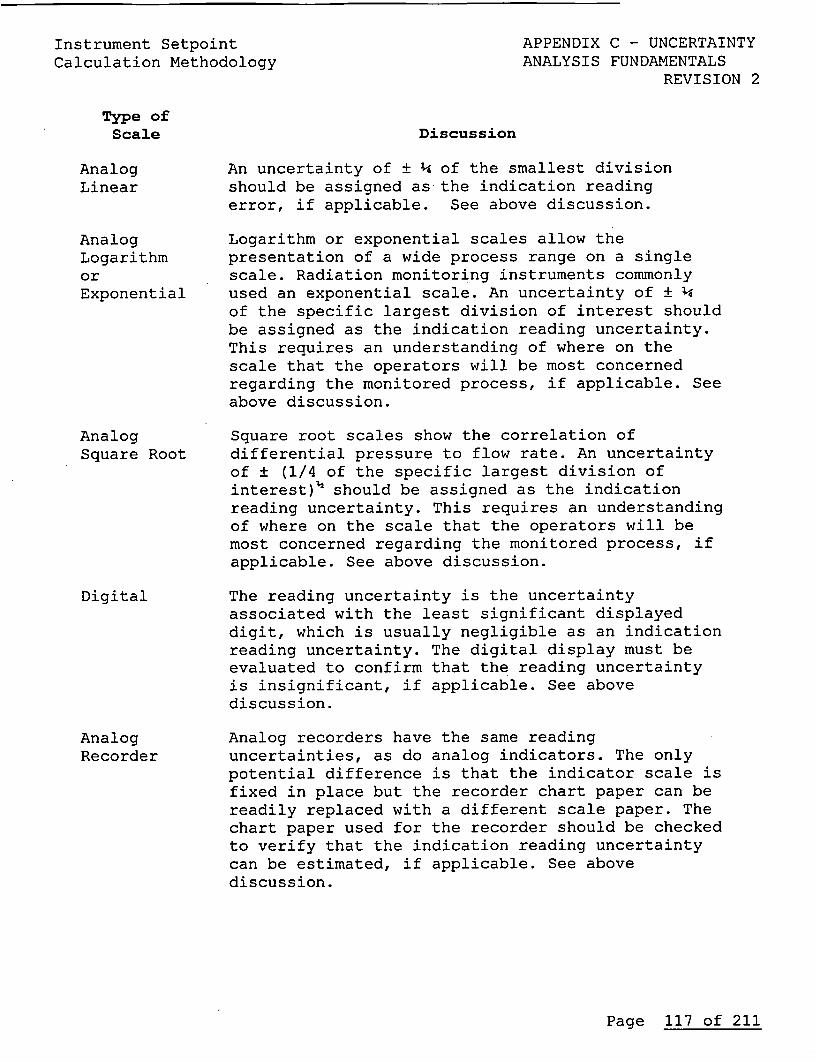
Instrument SetpointCalculation Methodology
Type ofScale
APPENDIX C - UNCERTAINTYANALYSIS FUNDAMENTALS
REVISION 2
Discussion
AnalogLinear
An uncertainty of ± 4 of the smallest divisionshould be assigned as the indication readingerror, if applicable. See above discussion.
AnalogLogarithmorExponential
AnalogSquare Root
Digital
AnalogRecorder
Logarithm or exponential scales allow thepresentation of a wide process range on a singlescale. Radiation monitoring instruments commonlyused an exponential scale. An uncertainty of ± kof the specific largest division of interest shouldbe assigned as the indication reading uncertainty.This requires an understanding of where on thescale that the operators will be most concernedregarding the monitored process, if applicable. Seeabove discussion.
Square root scales show the correlation ofdifferential pressure to flow rate. An uncertaintyof ± (1/4 of the specific largest division ofinterest)" should be assigned as the indicationreading uncertainty. This requires an understandingof where on the scale that the operators will bemost concerned regarding the monitored process, ifapplicable. See above discussion.
The reading uncertainty is the uncertaintyassociated with the least significant displayeddigit, which is usually negligible as an indicationreading uncertainty. The digital display must beevaluated to confirm that the reading uncertaintyis insignificant, if applicable. See abovediscussion.
Analog recorders have the same readinguncertainties, as do analog indicators. The onlypotential difference is that the indicator scale isfixed in place but the recorder chart paper can bereadily replaced with a different scale paper. Thechart paper used for the recorder should be checkedto verify that the indication reading uncertaintycan be estimated, if applicable. See abovediscussion.
Page 117 of 211
Instrument Setpoint APPENDIX C - UNCERTAINTYCalculation Methodology ANALYSIS FUNDAMENTALS
REVISION 2
C.3.14 Seismic Effects
Two types of seismic effects should be considered: 1) normaloperational vibration and minor seismic disturbances, and 2) designbasis seismic events in which certain equipment performs a safetyfunction.
The effects of normal vibration (or a minor seismic event that doesnot cause an unusual event) are assumed to be calibrated out on aperiodic basis and are considered negligible. Abnormal vibrations(vibration levels that produce noticeable effects) and moresignificant seismic events (severe enough to cause an unusualevent) are considered abnormal conditions that require maintenanceor equipment modification.
Design basis seismic events can cause a shift in an instrument'soutput. For the equipment that must function during and followinga design basis seismic or accident event, the environmentalqualification test report should be reviewed to obtain the boundinguncertainty. The seismic effect may be specified as a separateeffect or, in some cases, may be included in the overallenvironmental allowance. A seismic event coincident with a LOCAis a design basis event per USAR 15.6.5. However, per USAR15.6.5.1.1, there are no realistic, identifiable events which wouldresult in a pipe break inside the containment of the magnituderequired to cause a loss-of-coolant accident coincident with a safeshutdown earthquake. Therefore, each setpoint calculation shouldconsider the effects of a seismic event and loss-of-coolantaccident independently to establish the worst case scenario for theinstrumentation being evaluated. Consideration should be given tothe accident that the equipment is required to mitigate. Forexample, it is not necessary to impose LOCA conditions as worsecase if no credit is taken to mitigate a LOCA condition (e.g. atrip function may activate prior to any harsh environment, thuscalculation of LOCA is not required, whereas, indication may berequired LOCA/post LOCA, therefore both seismic and LOCA would becalculated and the worst value used). This consideration should bedocumented in the calculation.
For well-designed and properly mounted equipment, the seismiceffect will often contribute no more than ±0.5% to the overalluncertainty. This effect can be considered random and can beincluded within the uncertainty expression as a random term.Including a small allowance for seismic effects is considered aconservative, but not required, approach to the uncertaintyanalysis.
Page 118 of 211
Instrument Setpoint APPENDIX C - UNCERTAINTYCalculation Methodology ANALYSIS FUNDAMENTALS
REVISION 2C.3.15 Environmental Effects - Accident
The environmental allowance is intended to account for the effectsof high temperature, pressure, humidity, and radiation that mightbe present during an accident, such as a LOCA or HELB event. Thisallowance should include an evaluation of the timing of the eventincluding the environmental condition existing at the time thefunction is designed to trip (See example in C.3.14 above). Somemanufacturers do not distinguish the uncertainties due to each ofthe accident effects. In such cases, the accident uncertainty maybe a single ± value given for all accident effects.
Qualification reports for safety-related instruments normallycontain tables, graphs or both, of accuracy before, during andafter radiation and steam/pressure environmental and seismictesting. Many times, manufacturers summarize the results of thequalification testing in their product specification sheets. Moredetailed information is available in the equipment qualificationreport. The manufacturer's specification sheet tends to be veryconservative, as the worst-case performance result is normallypresented.
Because of the limited sample size typically used in qualificationtesting, the conservative approach to assigning uncertainty limitsis to use the bounding worst-case uncertainties. It is alsorecommended that discussions with the instrument manufacturer beconducted to gain insight into the behavior of the uncertainty(should it be considered random or bias?). This is importantbecause if the uncertainty is random and of approximately the samemagnitude as other random uncertainties, then SRSS methods might beused to combine the accident-induced uncertainty with otheruncertainties. The environmental allowance should be ofapproximately the same size as the other random uncertainties if itis combined with other random terms in an SRSS expression. Thisconsideration comes from the central limit theorem, which allowsthe combination of uncertainties by SRSS as long as they are ofapproximately the same magnitude. If not, then the accidentuncertainty should be treated as an arbitrarily distributeduncertainty.
Using data from the qualification report in place of performancespecifications, it is often possible to justify the use of loweruncertainty values that may occur at reduced temperatures orradiation dose levels. Typically, qualification tests are conductedat the upper extremes of simulated accident environments so thatthe results apply to as many plants as possible, each withdifferent requirements. Therefore, it is not always practical ornecessary to use the results at the bounding environmental extremeswhen the actual requirements are not as limiting. Some cautions areneeded, however, to preclude possible misapplication of the data:
Page 119 of 211
Instrument Setpoint APPENDIX C - UNCERTAINTYCalculation Methodology ANALYSIS FUNDAMENTALS
REVISION 21. The highest uncertainties of all the units tested at the
reduced temperatures or dose should be used. A margin shouldalso be applied to the tested magnitude of the environmentalparameter consistent with Institute of Electrical andElectronics Engineers 323-1975.
2. The units tested should have been tested under identical orequitable conditions and test sequences.
3. If data for a reduced temperature is used, ensure thatsufficient "soak-time" existed prior to the readings at thattemperature to ensure sufficient thermal equilibrium wasreached within the instrument case.
The requirement in Item (1) above is a conservative method toensure that bounding uncertainties are used in the absence of astatistically valid sample size. Item (2) above is an obviousrequirement for validity of this method. Item (3) ensures thatsufficient thermal lag time through the instrument case isaccounted for in drawing conclusions of performance at reducedtemperatures. In other words, if a transmitter case has a one-minute thermal lag time, then ensure that the transmitter was heldat the reduced temperature at least one minute prior to takingreadings.
Generally, the worst uncertainty is used from either thequalification report or the performance specification, unless moreconsideration is needed to preserve the existing AV or setpoint.
C.3.16 As-Left Tolerance Specification
The device as-left tolerance establishes the required accuracy bandthat a device or group of devices must be calibrated to withinwhen periodically tested. If an instrument as-found value is foundto be within the as-left tolerance, no further re-calibration isrequired for the instrument and calculations should assume that aninstrument might be left anywhere within this tolerance.
See Section 4.3.3 for establishing the calibration as-lefttolerance for a device. For all existing CPS instruments, an as-left tolerance is already specified by the applicable surveillancecalibration procedure. CPS typically calibrates non-safety relatedinstruments to a generic calibration procedure with tolerances perthe Instrument Data Sheet (IDS). This as-left tolerance isrecommended for use in the calculation unless other conditionssuggest that a different tolerance is warranted. For example, atighter tolerance is easily achievable for most electronicequipment and a tighter tolerance might provide needed margin for asetpoint calculation. Conversely, establishing a tighter tolerancethan is achievable per the manufacturer ensures that it willroutinely be found out of calibration.
Page 120 of 211
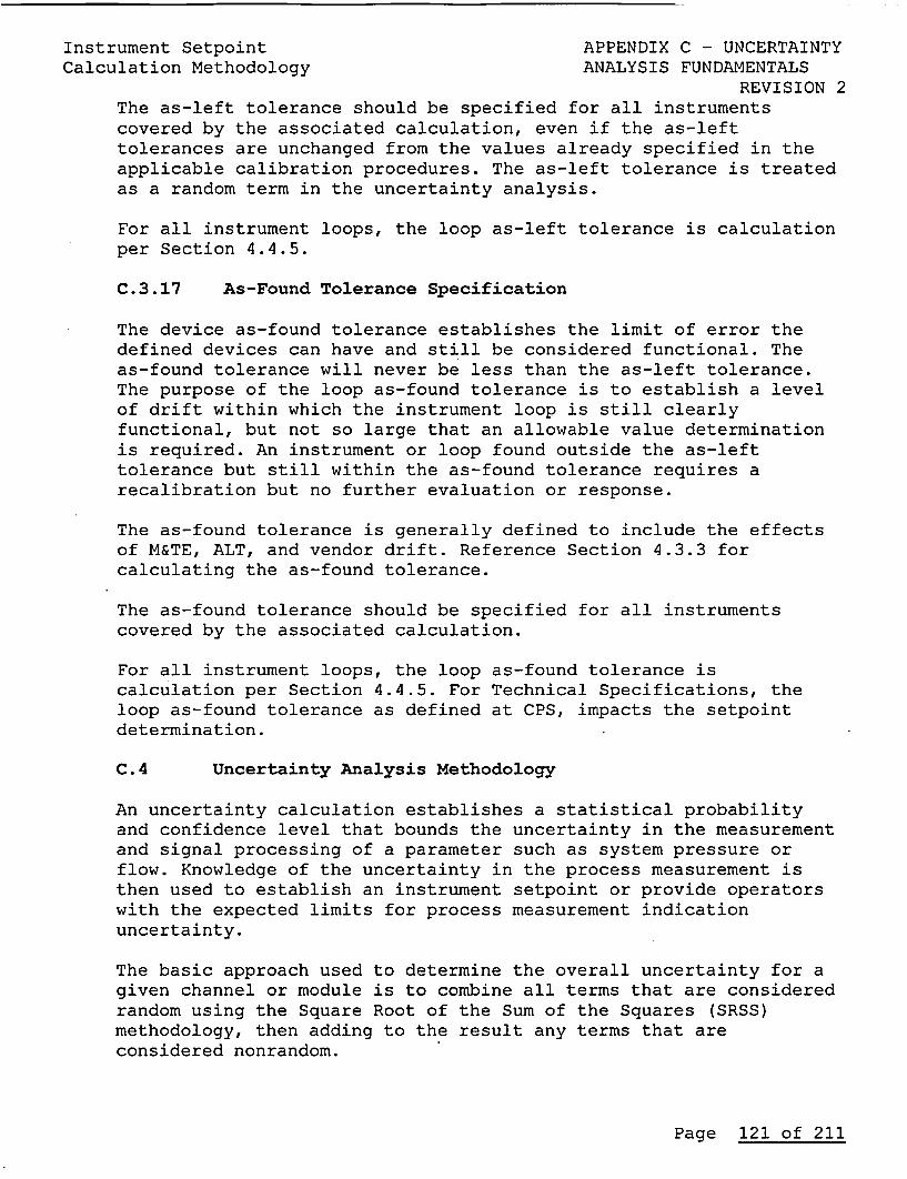
Instrument Setpoint APPENDIX C - UNCERTAINTYCalculation Methodology ANALYSIS FUNDAMENTALS
REVISION 2The as-left tolerance should be specified for all instrumentscovered by the associated calculation, even if the as-lefttolerances are unchanged from the values already specified in theapplicable calibration procedures. The as-left tolerance is treatedas a random term in the uncertainty analysis.
For all instrument loops, the loop as-left tolerance is calculationper Section 4.4.5.
C.3.17 As-Found Tolerance Specification
The device as-found tolerance establishes the limit of error thedefined devices can have and still be considered functional. Theas-found tolerance will never be less than the as-left tolerance.The purpose of the loop as-found tolerance is to establish a levelof drift within which the instrument loop is still clearlyfunctional, but not so large that an allowable value determinationis required. An instrument or loop found outside the as-lefttolerance but still within the as-found tolerance requires arecalibration but no further evaluation or response.
The as-found tolerance is generally defined to include the effectsof M&TE, ALT, and vendor drift. Reference Section 4.3.3 forcalculating the as-found tolerance.
The as-found tolerance should be specified for all instrumentscovered by the associated calculation.
For all instrument loops, the loop as-found tolerance iscalculation per Section 4.4.5. For Technical Specifications, theloop as-found tolerance as defined at CPS, impacts the setpointdetermination.
C.4 Uncertainty Analysis Methodology
An uncertainty calculation establishes a statistical probabilityand confidence level that bounds the uncertainty in the measurementand signal processing of a parameter such as system pressure orflow. Knowledge of the uncertainty in the process measurement isthen used to establish an instrument setpoint or provide operatorswith the expected limits for process measurement indicationuncertainty.
The basic approach used to determine the overall uncertainty for agiven channel or module is to combine all terms that are consideredrandom using the Square Root of the Sum of the Squares (SRSS)methodology, then adding to the result any terms that areconsidered nonrandom.
Page 121 of 211
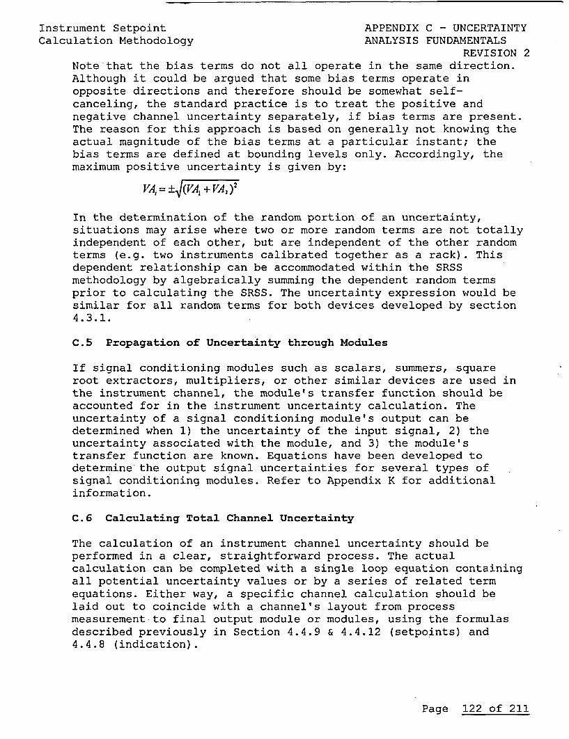
Instrument Setpoint APPENDIX C - UNCERTAINTYCalculation Methodology ANALYSIS FUNDAMENTALS
REVISION 2Note that the bias terms do not all operate in the same direction.Although it could be argued that some bias terms operate inopposite directions and therefore should be somewhat self-canceling, the standard practice is to treat the positive andnegative channel uncertainty separately, if bias terms are present.The reason for this approach is based on generally not knowing theactual magnitude of the bias terms at a particular instant; thebias terms are defined at bounding levels only. Accordingly, themaximum positive uncertainty is given by:
VAj= ±(VA, + VA2
In the determination of the random portion of an uncertainty,situations may arise where two or more random terms are not totallyindependent of each other, but are independent of the other randomterms (e.g. two instruments calibrated together as a rack). Thisdependent relationship can be accommodated within the SRSSmethodology by algebraically summing the dependent random termsprior to calculating the SRSS. The uncertainty expression would besimilar for all random terms for both devices developed by section4.3.1.
C.5 Propagation of Uncertainty through Modules
If signal conditioning modules such as scalars, summers, squareroot extractors, multipliers, or other similar devices are used inthe instrument channel, the module's transfer function should beaccounted for in the instrument uncertainty calculation. Theuncertainty of a signal conditioning module's output can bedetermined when 1) the uncertainty of the input signal, 2) theuncertainty associated with the module, and 3) the module'stransfer function are known. Equations have been developed todetermine the output signal uncertainties for several types ofsignal conditioning modules. Refer to Appendix K for additionalinformation.
C.6 Calculating Total Channel Uncertainty
The calculation of an instrument channel uncertainty should beperformed in a clear, straightforward process. The actualcalculation can be completed with a single loop equation containingall potential uncertainty values or by a series of related termequations. Either way, a specific channel calculation should belaid out to coincide with a channel's layout from processmeasurement to final output module or modules, using the formulasdescribed previously in Section 4.4.9 & 4.4.12 (setpoints) and4.4.8 (indication).
Page 122 of 211
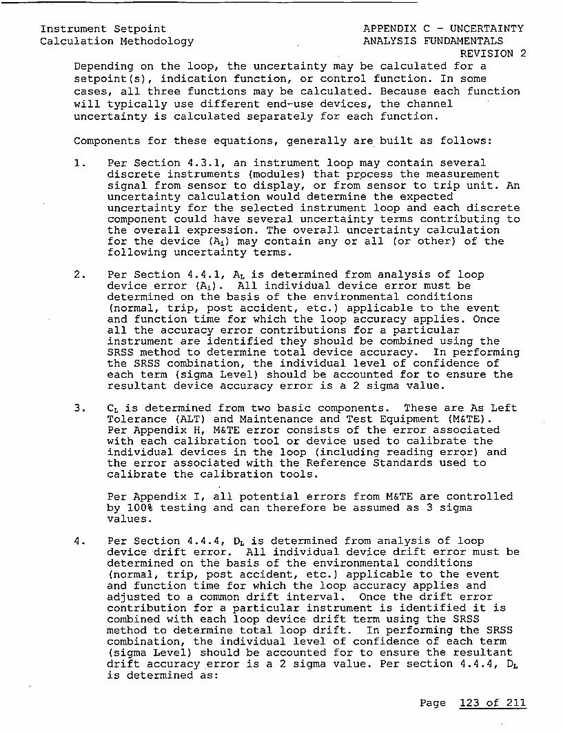
Instrument Setpoint APPENDIX C - UNCERTAINTYCalculation Methodology ANALYSIS FUNDAMENTALS
REVISION 2Depending on the loop, the uncertainty may be calculated for asetpoint(s), indication function, or control function. In somecases, all three functions may be calculated. Because each functionwill typically use different end-use devices, the channeluncertainty is calculated separately for each function.
Components for these equations, generally are built as follows:
1. Per Section 4.3.1, an instrument loop may contain severaldiscrete instruments (modules) that process the measurementsignal from sensor to display, or from sensor to trip unit. Anuncertainty calculation would determine the expecteduncertainty for the selected instrument loop and each discretecomponent could have several uncertainty terms contributing tothe overall expression. The overall uncertainty calculationfor the device (Ai) may contain any or all (or other) of thefollowing uncertainty terms.
2. Per Section 4.4.1, AL is determined from analysis of loopdevice error (Ai). All individual device error must bedetermined on the basis of the environmental conditions(normal, trip, post accident, etc.) applicable to the eventand function time for which the loop accuracy applies. Onceall the accuracy error contributions for a particularinstrument are identified they should be combined using theSRSS method to determine total device accuracy. In performingthe SRSS combination, the individual level of confidence ofeach term (sigma Level) should be accounted for to ensure theresultant device accuracy error is a 2 sigma value.
3. CL is determined from two basic components. These are As LeftTolerance (ALT) and Maintenance and Test Equipment (M&TE).Per Appendix H, M&TE error consists of the error associatedwith each calibration tool or device used to calibrate theindividual devices in the loop (including reading error) andthe error associated with the Reference Standards used tocalibrate the calibration tools.
Per Appendix I, all potential errors from M&TE are controlledby 100% testing and can therefore be assumed as 3 sigmavalues.
4. Per Section 4.4.4, DL is determined from analysis of loopdevice drift error. All individual device drift error must bedetermined on the basis of the environmental conditions(normal, trip, post accident, etc.) applicable to the eventand function time for which the loop accuracy applies andadjusted to a common drift interval. Once the drift errorcontribution for a particular instrument is identified it iscombined with each loop device drift term using the SRSSmethod to determine total loop drift. In performing the SRSScombination, the individual level of confidence of each term(sigma Level) should be accounted for to ensure the resultantdrift accuracy error is a 2 sigma value. Per section 4.4.4, DL
is determined as:
Page 123 of 211

Instrument Setpoint APPENDIX C - UNCERTAINTYCalculation Methodology ANALYSIS FUNDAMENTALS
REVISION 2
5. Per Sections 4.4.6, C.3.1, and C.3.2, PMA and PEA areestablished as uncertainties to account for measurementerrors, which lie outside the normal calibration bounds of thechannel.
6. Per Section 4.4.8.2, the biases for all modules should beaccounted for and combined outside the square root radical.
Page 124 of 211
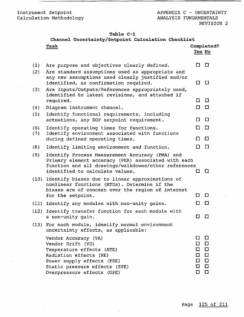
Instrument Setpoint APPENDIX C - UNCERTAINTYCalculation Methodology ANALYSIS FUNDAMENTALS
REVISION 2
Table C-1Channel Uncertainty/Setpoint Calculation Checklist
Task Completed?Yes No
(1) Are purpose and objectives clearly defined. 0 0(2) Are standard assumptions used as appropriate and
any new assumptions used clearly justified and/oridentified, as confirmation required. E 0
(3) Are Inputs/Outputs/References appropriately used,identified to latest revisions, and attached ifrequired. 0 0
(4) Diagram instrument channel. 0 0(5) Identify functional requirements, including
actuations, any EOP setpoint requirement. E El
(6) Identify operating times for functions. El 0(7) Identify environment associated with functions
during defined operating times. 0 0
(8) Identify limiting environment and function. 0 0
(9) Identify Process Measurement Accuracy (PMA) andPrimary element accuracy (PEA) associated with eachfunction and all drawings/walkdowns/other references.identified to calculate values. 00
(10) Identify biases due to linear approximations ofnonlinear functions (RTDs). Determine if thebiases are of concern over the region of interestfor the setpoint. 0 0
(11) Identify any modules with non-unity gains. 0 0
(12) Identify transfer function for each module witha non-unity gain. l 0
(13) For each module, identify normal environmentuncertainty effects, as applicable:
Vendor Accuracy (VA) 00Vendor Drift (VD) 0 0Temperature effects (ATE) 0 0Radiation effects (RE) 0 0Power supply effects (PSE) 0 0Static pressure effects (SPE) 0 0Overpressure effects (OPE) 0 0
Page 125 of 211
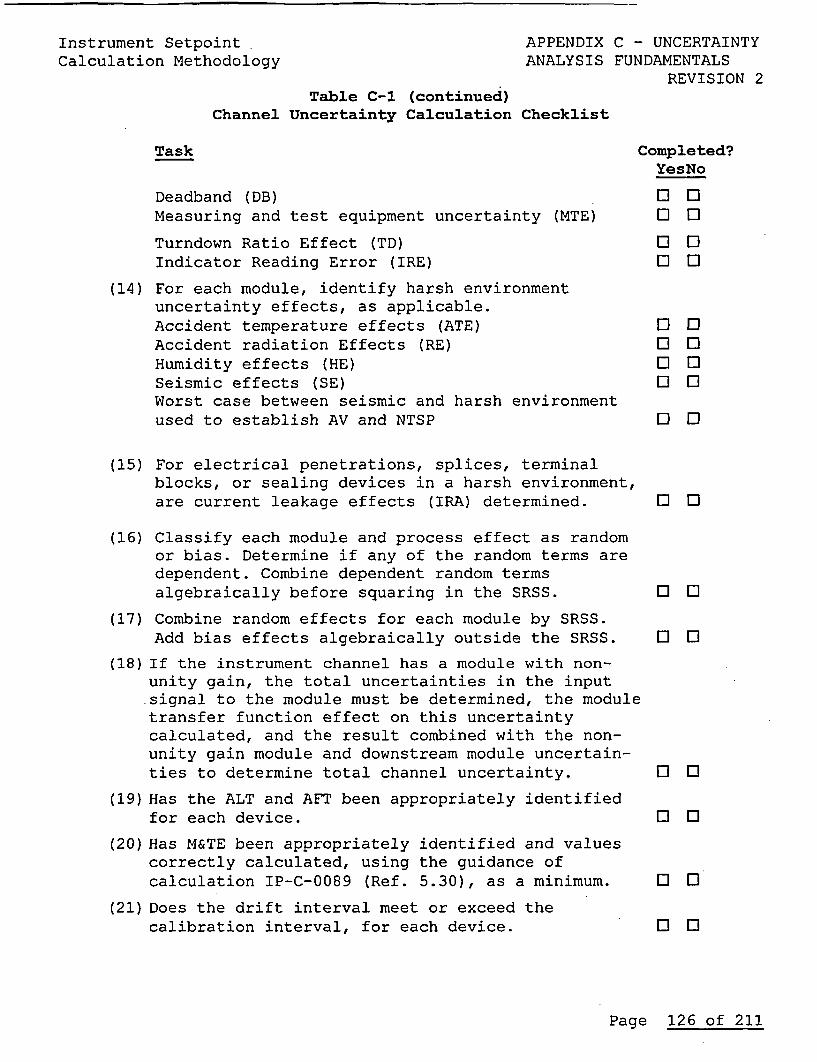
Instrument Setpoint APPENDIX C - UNCERTAINTYCalculation Methodology ANALYSIS FUNDAMENTALS
REVISION 2Table C-1 (continued)
Channel Uncertainty Calculation Checklist
Task Completed?YesNo
Deadband (DB) 00Measuring and test equipment uncertainty (MTE) 0 0
Turndown Ratio Effect (TD) 00Indicator Reading Error (IRE) 0 0
(14) For each module, identify harsh environmentuncertainty effects, as applicable.Accident temperature effects (ATE) 0 0Accident radiation Effects (RE) 0 0Humidity effects (HE) 0 0Seismic effects (SE) 0 0Worst case between seismic and harsh environmentused to establish AV and NTSP 00
(15) For electrical penetrations, splices, terminalblocks, or sealing devices in a harsh environment,are current leakage effects (IRA) determined. 0 0
(16) Classify each module and process effect as randomor bias. Determine if any of the random terms aredependent. Combine dependent random termsalgebraically before squaring in the SRSS. 0 0
(17) Combine random effects for each module by SRSS.Add bias effects algebraically outside the SRSS. 0 0
(18)If the instrument channel has a module with non-unity gain, the total uncertainties in the inputsignal to the module must be determined, the moduletransfer function effect on this uncertaintycalculated, and the result combined with the non-unity gain module and downstream module uncertain-ties to determine total channel uncertainty. 0 0
(19)Has the ALT and AFT been appropriately identifiedfor each device. 0 0
(20)Has M&TE been appropriately identified and valuescorrectly calculated, using the guidance ofcalculation IP-C-0089 (Ref. 5.30), as a minimum. 0 0
(21) Does the drift interval meet or exceed thecalibration interval, for each device. 0 0
Page 126 of 211
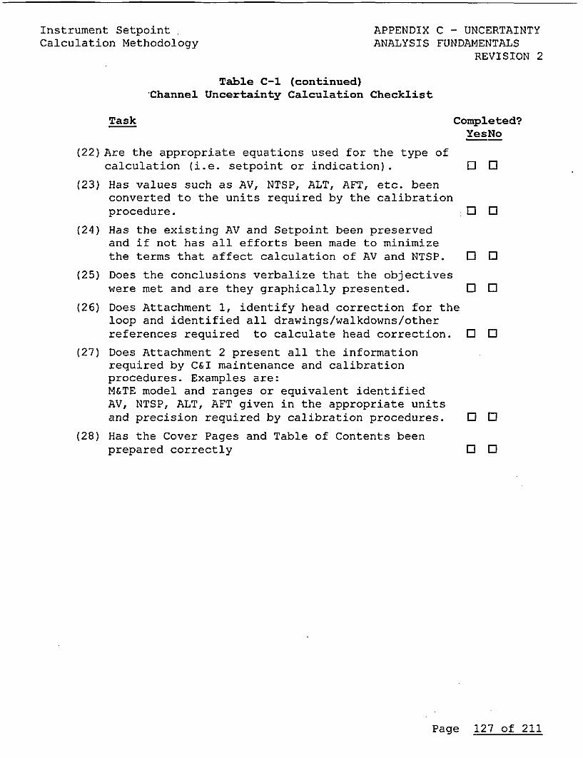
Instrument Setpoint APPENDIX C - UNCERTAINTYCalculation Methodology ANALYSIS FUNDAMENTALS
REVISION 2
Table C-1 (continued)Channel Uncertainty Calculation Checklist
Task Completed?YesNo
(22)Are the appropriate equations used for the type ofcalculation (i.e. setpoint or indication). 0 0
(23) Has values such as AV, NTSP, ALT, AFT, etc. beenconverted to the units required by the calibrationprocedure. 0 0
(24) Has the existing AV and Setpoint been preservedand if not has all efforts been made to minimizethe terms that affect calculation of AV and NTSP. 0 El
(25) Does the conclusions verbalize that the objectiveswere met and are they graphically presented. 0 El
(26) Does Attachment 1, identify head correction for theloop and identified all drawings/walkdowns/otherreferences required to calculate head correction. O 0
(27) Does Attachment 2 present all the informationrequired by C&I maintenance and calibrationprocedures. Examples are:M&TE model and ranges or equivalent identifiedAV, NTSP, ALT, AFT given in the appropriate unitsand precision required by calibration procedures. El E
(28) Has the Cover Pages and Table of Contents beenprepared correctly 0 0
Page 127 of 211
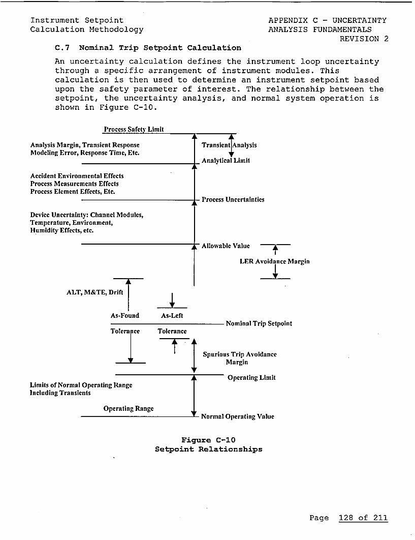
Instrument Setpoint APPENDIX C - UNCERTAINTYCalculation Methodology ANALYSIS FUNDAMENTALS
REVISION 2C.7 Nominal Trip Setpoint Calculation
An uncertainty calculation defines the instrument loop uncertaintythrough a specific arrangement of instrument modules. Thiscalculation is then used to determine an instrument setpoint basedupon the safety parameter of interest. The relationship between thesetpoint, the uncertainty analysis, and normal system operation isshown in Figure C-10.
Process Safety Limit
Analysis Margin, Transient Response Transient AnalysisModeling Error, Response Time, Etc.
_ Analytical Limit
Accident Environmental EffectsProcess Measurements EffectsProcess Element Effects, Etc.
- Process Uncertainties
Device Uncertainty: Channel Modules,Temperature, Environment,Humidity Effects, etc.
X - Allowable Value
LER Avoidance Margin
ALT, M&TE, Drift
As-Found As-LeftNominal Trip Setpoint
Tolerance Tolerance
_TiiVt Spurious Trip Avoidance
Margin
Operating LimitLimits of Normal Operating RangeIncluding Transients
Operating RangeNormal Operating Value
Figure C-10Setpoint Relationships
Page 128 of 211
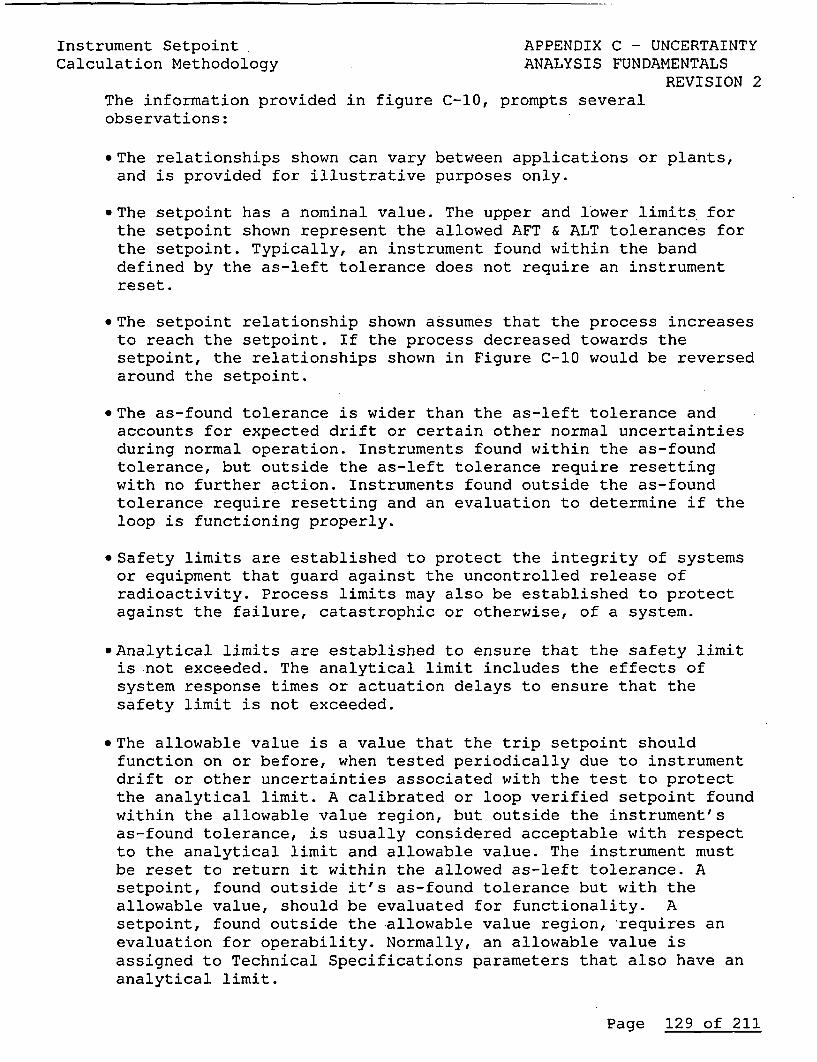
Instrument Setpoint APPENDIX C - UNCERTAINTYCalculation Methodology ANALYSIS FUNDAMENTALS
REVISION 2The information provided in figure C-10, prompts severalobservations:
*The relationships shown can vary between applications or plants,and is provided for illustrative purposes only.
*The setpoint has a nominal value. The upper and lower limits forthe setpoint shown represent the allowed AFT & ALT tolerances forthe setpoint. Typically, an instrument found within the banddefined by the as-left tolerance does not require an instrumentreset.
*The setpoint relationship shown assumes that the process increasesto reach the setpoint. If the process decreased towards thesetpoint, the relationships shown in Figure C-10 would be reversedaround the setpoint.
*The as-found tolerance is wider than the as-left tolerance andaccounts for expected drift or certain other normal uncertaintiesduring normal operation. Instruments found within the as-foundtolerance, but outside the as-left tolerance require resettingwith no further action. Instruments found outside the as-foundtolerance require resetting and an evaluation to determine if theloop is functioning properly.
*Safety limits are established to protect the integrity of systemsor equipment that guard against the uncontrolled release ofradioactivity. Process limits may also be established to protectagainst the failure, catastrophic or otherwise, of a system.
&Analytical limits are established to ensure that the safety limitis not exceeded. The analytical limit includes the effects ofsystem response times or actuation delays to ensure that thesafety limit is not exceeded.
'The allowable value is a value that the trip setpoint shouldfunction on or before, when tested periodically due to instrumentdrift or other uncertainties associated with the test to protectthe analytical limit. A calibrated or loop verified setpoint foundwithin the allowable value region, but outside the instrument'sas-found tolerance, is usually considered acceptable with respectto the analytical limit and allowable value. The instrument mustbe reset to return it within the allowed as-left tolerance. Asetpoint, found outside it's as-found tolerance but with theallowable value, should be evaluated for functionality. Asetpoint, found outside the allowable value region, requires anevaluation for operability. Normally, an allowable value isassigned to Technical Specifications parameters that also have ananalytical limit.
Page 129 of 211
Instrument Setpoint APPENDIX C - UNCERTAINTYCalculation Methodology ANALYSIS FUNDAMENTALS
REVISION 2
*The trip setpoint is the desired actuation point that ensures,when all known sources of measurement uncertainty are included,that an analytical limit is not exceeded. Depending on thesetpoint, additional margin may exist between the trip setpointand the analytical limit. The trip setpoint is selected to ensurethe analytical limit is not exceeded while also minimizing thepossibility of inadvertent actuations during normal plantoperation.
Page 130 of 211
Instrument Setpoint APPENDIX D - EFFECT OF INSULATIONCalculation Methodology RESISTANCE ON UNCERTAINTY
REVISION 2
APPENDIX DEFFECT OF INSULATION RESISTANCE ON UNCERTAINTY
D.1 Background
Under the conditions of high humidity and temperature associatedwith either a Loss of Coolant Accident (LOCA) or high energy linebreak (HELB), the insulation resistance (IR) may decrease ininstrument loop components such as cables, splices, connectors,containment penetrations, and terminal blocks. A decrease in IRresults in an increase in instrument loop leakage current and acorresponding increase in measurement uncertainty of the processparameters, defined in Section 2.2 as IRA.
Degraded IR effects during a LOCA or HELB are a concern forinstrumentation circuits due to the low signal current levels. Adecrease in IR can result in substantial current leakage thatshould be accounted for in instrument setpoint and post accidentmonitoring uncertainty calculations. The NRC expressed concern withterminal block leakage currents in Information Notice 84-47. Morerecently, the NRC stated in Information Notice 92-12 (Ref. 5.12)that leakage currents should be considered for certain instrumentsetpoints and indication.
This Appendix provides an overview of IR effects on standardinstrumentation circuits and provides examples of the effect of IRAon instrument uncertainty. Specifically, this Appendix addressesthe following:
oQualitative effects of temperature and humidity on IR*Analytical methodology for evaluating IR effects on instrumentloop performance
*Technical information needed to perform an evaluation*Application of results to uncertainty calculations*Consideration of inherent margins in the analytical methodology
Page 131 of 211
Instrument Setpoint APPENDIX D - EFFECT OF INSULATIONCalculation Methodology RESISTANCE ON UNCERTAINTY
REVISION 2
D.2 Environmental Effects on Insulation Resistance
IR is affected by changes in the environment. ASTM Standard D257-91(Ref. 5.31), provides a discussion of the factors that affect theresistance of a material. This ASTM standard discusses materialproperties in general; it does not limit itself to cables or anyother type of particular construction. Factors that affect theresistance or the ability to measure resistance include:
*Temperature'Humidity'Time of electrification (electrical measurement of resistance)
*Magnitude of voltage*Contour of specimen'Measuring circuit deficiencies*Residual charge
Temperature and humidity effects are of particular interest forcircuits that may be exposed to an accident harsh environment. Theresistance of an organic insulating material changes exponentiallywith temperature. Often, this variation can be represented in theform:
R = Be- (MIT).
where,
.R =Resistance of an insulating materialB =Proportionality constantm =Activation constantT =Absolute temperature in degrees Kelvin
One manufacturer predicts a similar exponential variation of IRwith respect to temperature for their cable; the manufacturerprovides the following equation, for determining IR at a giventemperature:
IR = (4 x 10¹⁵) log (D/d) e(- 0 0 79 X T)
where,
IR Calculated cable insulation resistance, megohm for 1,000 ftT = Temperature, degrees Kelvind = Diameter of conductorD = Diameter of conductor and insulation
Page 132 of 211
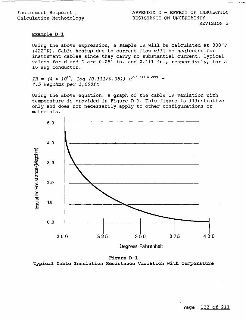
- - - -
Instrument SetpointCalculation Methodology
APPENDIX D - EFFECT OF INSULATIONRESISTANCE ON UNCERTAINTY
REVISION 2
Example D-1
Using the above expression, a sample IR will be calculated at 3000 F(4220K). Cable heatup due to current flow will be neglected forinstrument cables since they carry no substantial current. Typicalvalues for d and D are 0.051 in. and 0.111 in., respectively, for a16 awg conductor.
IR = (4 X 10¹⁵) log (0.111/0.051) e(-0 .0 7 9 X 422) =
4.5 megohms per 1,OOOft
Using the above equation, a graph of the cable IR variation withtemperature is provided in Figure D-1. This figure is illustrativeonly and does not necessarily apply to other configurations ormaterials.
5.0
4.0
2
3.0
2.0
1.0
I I0 .0
300
Degrees Fahrenheit
Figure D-1Typical Cable Insulation Resistance Variation with Temperature
Page 133 of 211
Instrument Setpoint APPENDIX D - EFFECT OF INSULATIONCalculation Methodology RESISTANCE ON UNCERTAINTY
REVISION 2
Insulation resistance of solid dielectric materials decreases withincreasing temperature and with increasing humidity. Volumeresistance of the insulating material is particularly sensitive totemperature changes. Surface resistance changes widely and veryrapidly with humidity changes. In both cases, the change in IRoccurs exponentially.
ASTM D257, Reference 5.31, discusses temperature and humidity as acombined effect on IR. In some materials, a change from 250 C to1000C may change IR by a factor of 100,000 due to the combinedeffects of temperature and humidity. The effect of temperaturealone is usually much smaller.
IR is a function of the volume resistance as well as the surfaceresistance of the material. In the case of an EQ test that includessteam and elevated temperatures, the minimum IR is expected nearthe peak of the temperature transient in a steam environment.Condensation of steam and chemical spray products will reduce thesurface resistance substantially.
Page 134 of 211
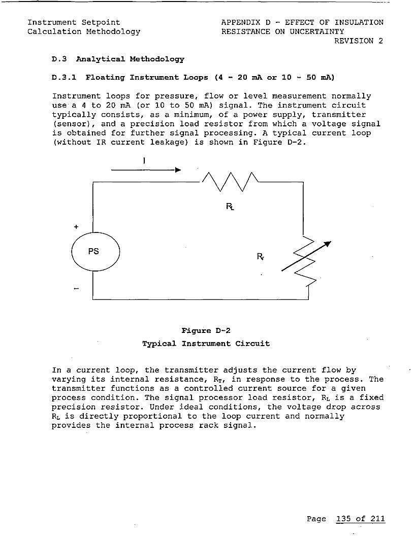
Instrument SetpointCalculation Methodology
APPENDIX D - EFFECT OF INSULATIONRESISTANCE ON UNCERTAINTY
REVISION 2
D.3 Analytical Methodology
D.3.1 Floating Instrument Loops (4 - 20 mA or 10 - 50 mA)
Instrument loops for pressure, flow or level measurement normallyuse a 4 to 20 mA (or 10 to 50 mA) signal. The instrument circuittypically consists, as a minimum, of a power supply, transmitter(sensor), and a precision load resistor from which a voltage signalis obtained for further signal processing. A typical current loop(without IR current leakage) is shown in Figure D-2.
Figure D-2
Typical Instrument Circuit
In a current loop, the transmitter adjusts the current flow byvarying its internal resistance, RT, in response to the process. Thetransmitter functions as a controlled current source for a givenprocess condition. The signal processor load resistor, RL is a fixedprecision resistor. Under ideal conditions, the voltage drop acrossRL is directly proportional to the loop current and normallyprovides the internal process rack signal.
Page 135 of 211
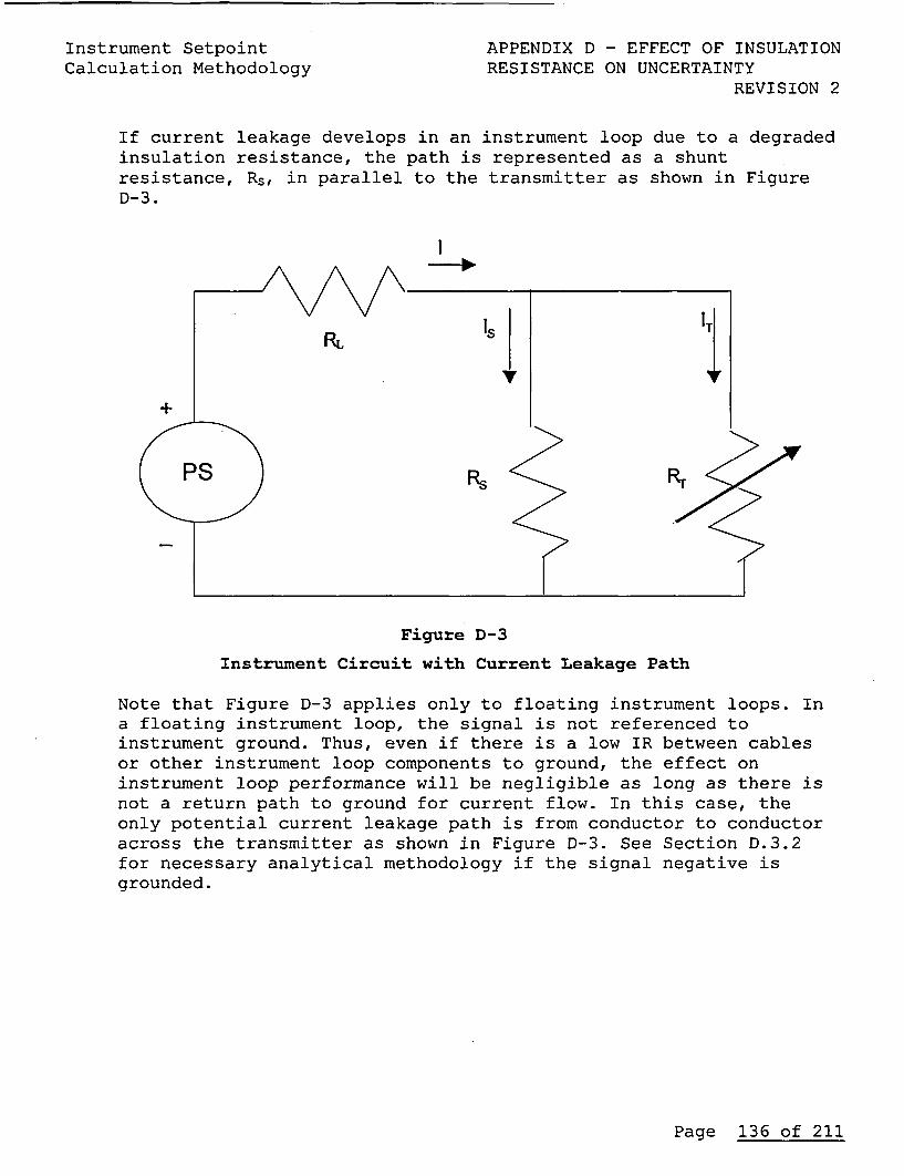
Instrument SetpointCalculation Methodology
APPENDIX D - EFFECT OF INSULATIONRESISTANCE ON UNCERTAINTY
REVISION 2
If current leakage develops in an instrument loop due to a degradedinsulation resistance, the path is represented as a shuntresistance, Rs, in parallel to the transmitter as shown in FigureD-3.
Figure D-3
Instrument Circuit with Current Leakage Path
Note that Figure D-3 applies only to floating instrument loops. Ina floating instrument loop, the signal is not referenced toinstrument ground. Thus, even if there is a low IR between cablesor other instrument loop components to ground, the effect oninstrument loop performance will be negligible as long as there isnot a return path to ground for current flow. In this case, theonly potential current leakage path is from conductor to conductoracross the transmitter as shown in Figure D-3. See Section D.3.2for necessary analytical methodology if the signal negative isgrounded.
Page 136 of 211
Instrument Setpoint APPENDIX D - EFFECT OF INSULATIONCalculation Methodology RESISTANCE ON UNCERTAINTY
REVISION 2Leakage current disrupts the one-to-one relationship between thetransmitter current and load current, such that a measurement erroris introduced at the load. For a standard 4 - 20 mA (or 10 to 50mA) instrument loop, the error is always in the higher-than-actualdirection, meaning that the load current will be higher than thetransmitter output current. The magnitude of the error in percentspan (Is(e)) caused by leakage is defined as the ratio of leakagecurrent to the 16mA span of a 4 - 2OmA loop, or,
Is = (IS/1 6mA) x 100
Where Is = shunt current
From figure D-3, Is can be expressed in terms of voltage, currentand resistance in the current loop consisting of a power supply,load resistance and IR (shunt resistance) as follows:
V = IL RL + Is Rs
where,V Power supply voltageIL = Current through the load resistorIs = Shunt currentRL = Rack load resistanceRs = Equivalent shunt (IR) resistance
Solving for Is,
Is = (V - IL RL) /Rs
Converting mA to Amps and normalizing for a 16mA span yields thefollowing result:
Is (* span) = [ (V - IL RL )/(R 5 X 0. 016) ] x 100
The error due to current leakage is inversely proportional to theIR, or Rs in the above equation. As Rs decreases, the loop error dueto current leakage increases. Note that equation to determine "V"has been simplified to provide an error in terms of percent span.For this case, the total instrument span is 16 mA for a 4 to 20 mAinstrument loop.
Rs is an equivalent shunt resistance obtained from several parallelshunt paths. A typical circuit inside containment, showing allpotential parallel current leakage paths, is shown in Figure D-4.
Page 137 of 211
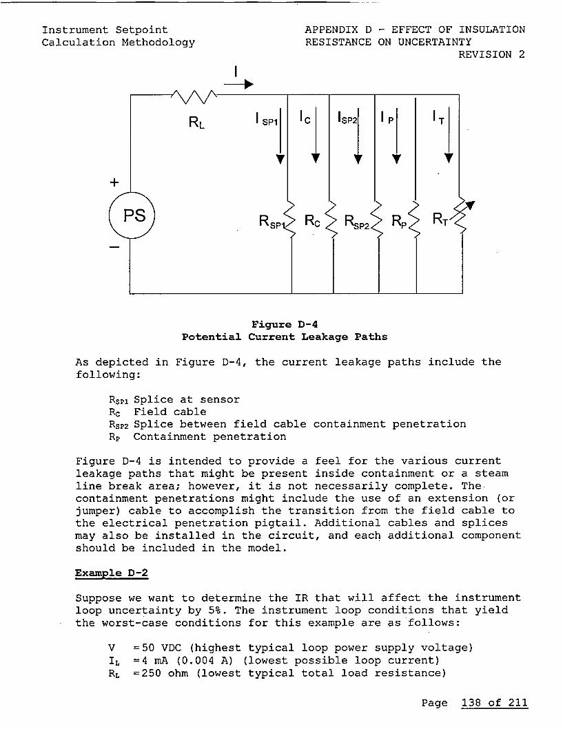
Instrument SetpointCalculation Methodology
APPENDIX D - EFFECT OF INSULATIONRESISTANCE ON UNCERTAINTY
REVISION 2
I
I
Figure D-4Potential Current Leakage Paths
As depicted in Figure D-4, the current leakage paths include thefollowing:
Rsp, Splice at sensorRc Field cableRsP2 Splice between field cable containment penetrationRp Containment penetration
Figure D-4 is intended to provide a feel for the various currentleakage paths that might be present inside containment or a steamline break area; however, it is not necessarily complete. Thecontainment penetrations might include the use of an extension (orjumper) cable to accomplish the transition from the field cable tothe electrical penetration pigtail. Additional cables and splicesmay also be installed in the circuit, and each additional componentshould be included in the model.
Example D-2
Suppose we want to determine the IR that will affect the instrumentloop uncertainty by 5%. The instrument loop conditions that yieldthe worst-case conditions for this example are as follows:
V =50 VDC (highest typical loop power supply voltage)IL =4 mA (0.004 A) (lowest possible loop current)RL =250 ohm (lowest typical total load resistance)
Page 138 of 211
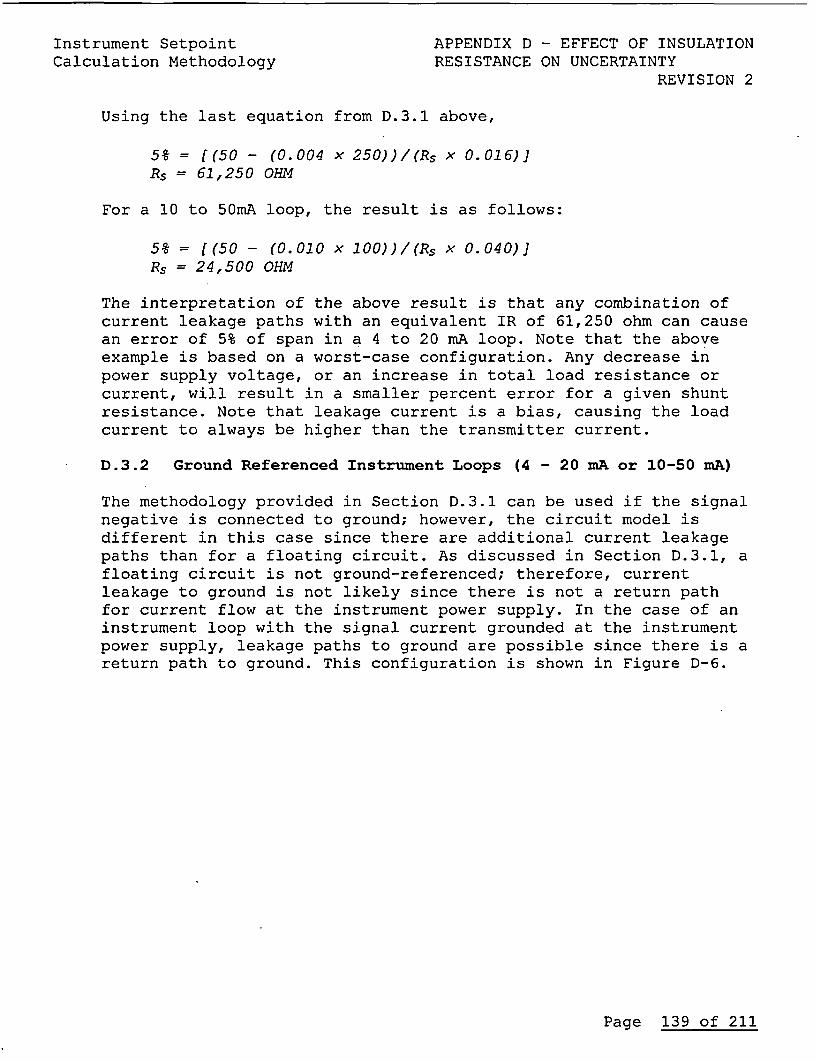
Instrument Setpoint APPENDIX D - EFFECT OF INSULATIONCalculation Methodology RESISTANCE ON UNCERTAINTY
REVISION 2
Using the last equation from D.3.1 above,
5% = [(50 - (0. 004 x 250)) / (Rs x 0. 016)]Rs= 61,250 OHM
For a 10 to 5OmA loop, the result is as follows:
5* [(50 - (0.010 x 100))/(Rs x 0.040)]Rs= 24,500 OHM
The interpretation of the above result is that any combination ofcurrent leakage paths with an equivalent IR of 61,250 ohm can causean error of 5% of span in a 4 to 20 mA loop. Note that the aboveexample is based on a worst-case configuration. Any decrease inpower supply voltage, or an increase in total load resistance orcurrent, will result in a smaller percent error for a given shuntresistance. Note that leakage current is a bias, causing the loadcurrent to always be higher than the transmitter current.
D.3.2 Ground Referenced Instrument Loops (4 - 20 mA or 10-50 mA)
The methodology provided in Section D.3.1 can be used if the signalnegative is connected to ground; however, the circuit model isdifferent in this case since there are additional current leakagepaths than for a floating circuit. As discussed in Section D.3.1, afloating circuit is not ground-referenced; therefore, currentleakage to ground is not likely since there is not a return pathfor current flow at the instrument power supply. In the case of aninstrument loop with the signal current grounded at the instrumentpower supply, leakage paths to ground are possible since there is areturn path to ground. This configuration is shown in Figure D-6.
Page 139 of 211
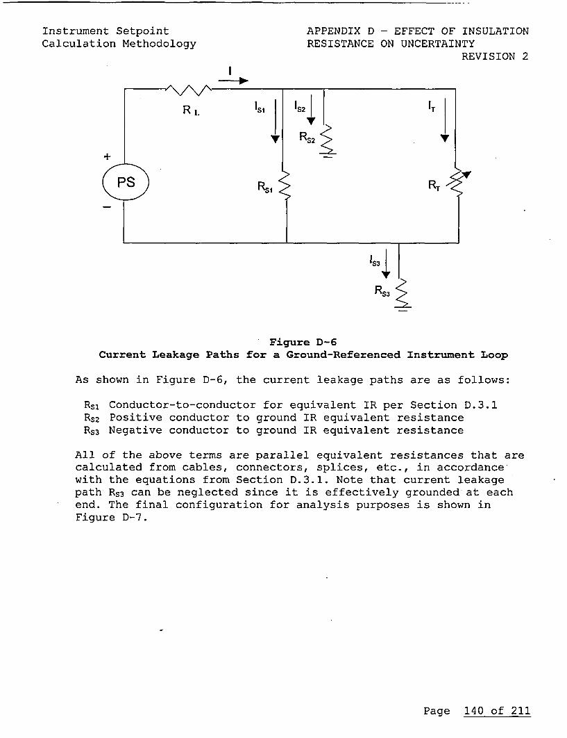
Instrument SetpointCalculation Methodology
APPENDIX D - EFFECT OF INSULATIONRESISTANCE ON UNCERTAINTY
REVISION 2
I
Figure D-6Current Leakage Paths for a Ground-Referenced Instrument Loop
As shown in Figure D-6, the current leakage paths are as follows:
Rs, Conductor-to-conductor for equivalent IR per Section D.3.1RS2 Positive conductor to ground IR equivalent resistanceRs3 Negative conductor to ground IR equivalent resistance
All of the above terms are parallel equivalent resistances that arecalculated from cables, connectors, splices, etc., in accordancewith the equations from Section D.3.1. Note that current leakagepath Rs3 can be neglected since it is effectively grounded at eachend. The final configuration for analysis purposes is shown inFigure D-7.
Page 140 of 211
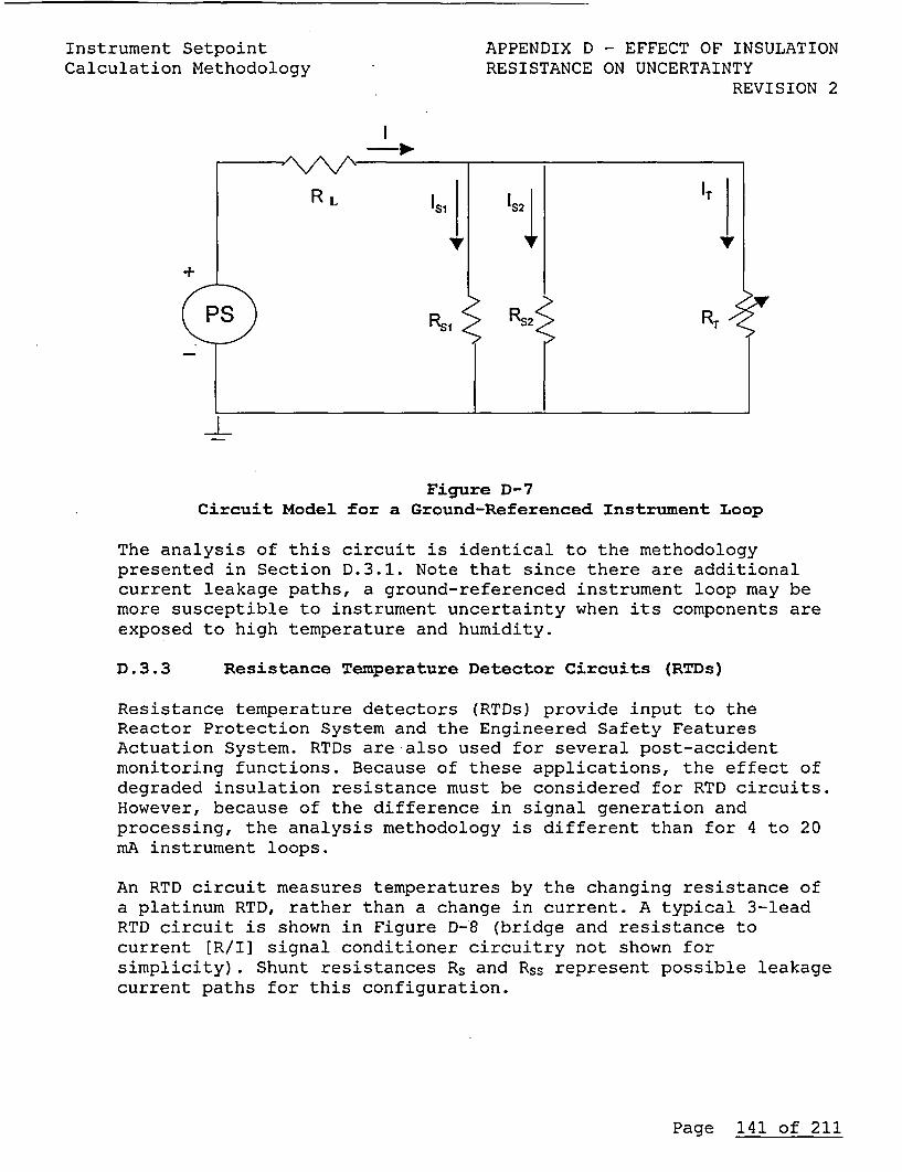
Instrument SetpointCalculation Methodology
APPENDIX D - EFFECT OF INSULATIONRESISTANCE ON UNCERTAINTY
REVISION 2
IP.
Figure D-7Circuit Model for a Ground-Referenced Instrument Loop
The analysis of this circuit is identical to the methodologypresented in Section D.3.1. Note that since there are additionalcurrent leakage paths, a ground-referenced instrument loop may bemore susceptible to instrument uncertainty when its components areexposed to high temperature and humidity.
D.3.3 Resistance Temperature Detector Circuits (RTDs)
Resistance temperature detectors (RTDs) provide input to theReactor Protection System and the Engineered Safety FeaturesActuation System. RTDs are also used for several post-accidentmonitoring functions. Because of these applications, the effect ofdegraded insulation resistance must be considered for RTD circuits.However, because of the difference in signal generation andprocessing, the analysis methodology is different than for 4 to 20mA instrument loops.
An RTD circuit measures temperatures by the changing resistance ofa platinum RTD, rather than a change in current. A typical 3-leadRTD circuit is shown in Figure D-8 (bridge and resistance tocurrent [R/I] signal conditioner circuitry not shown forsimplicity). Shunt resistances Rs and Rss represent possible leakagecurrent paths for this configuration.
Page 141 of 211
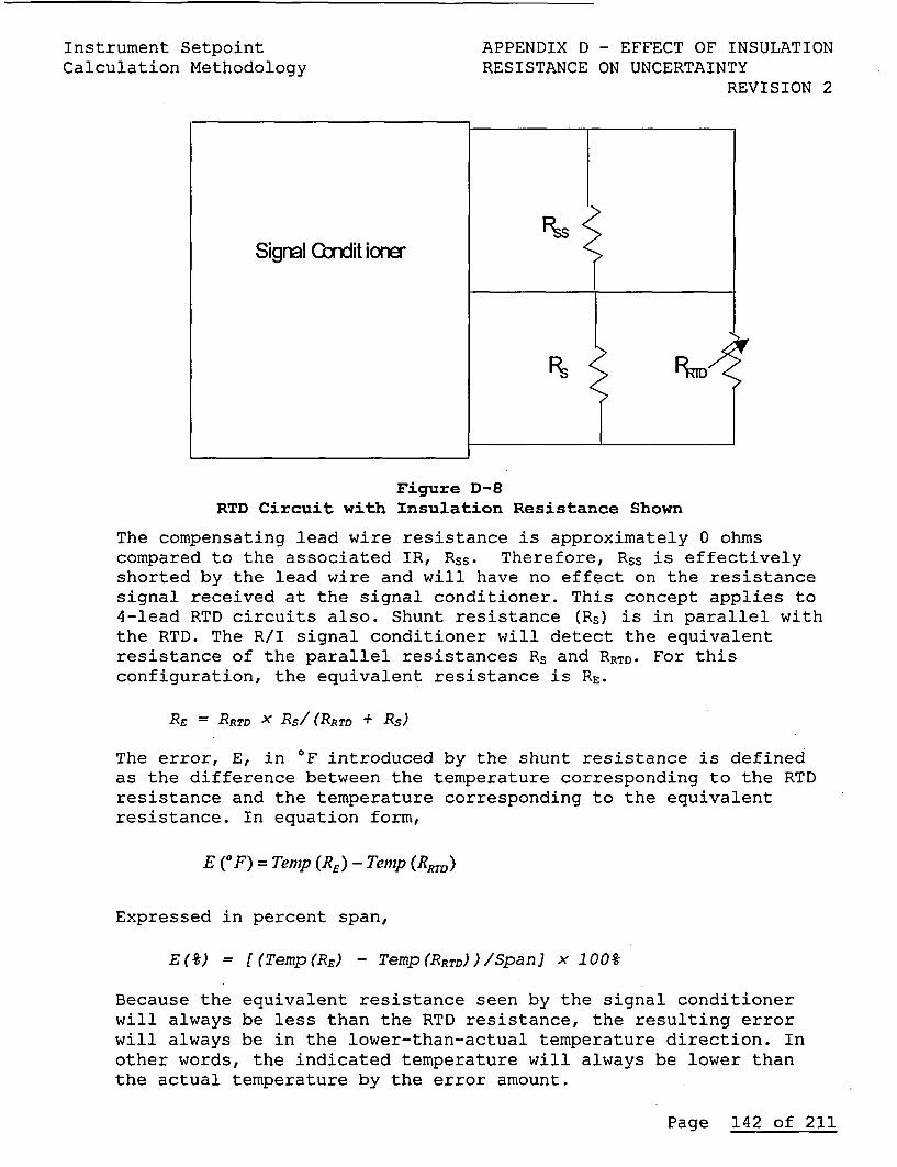
Instrument SetpointCalculation Methodology
APPENDIX D - EFFECT OF INSULATIONRESISTANCE ON UNCERTAINTY
REVISION 2
Figure D-8RTD Circuit with Insulation Resistance Shown
The compensating lead wire resistance is approximately 0 ohmscompared to the associated IR, Rss. Therefore, Rss is effectivelyshorted by the lead wire and will have no effect on the resistancesignal received at the signal conditioner. This concept applies to4-lead RTD circuits also. Shunt resistance (Rs) is in parallel withthe RTD. The R/I signal conditioner will detect the equivalentresistance of the parallel resistances Rs and RRTD. For thisconfiguration, the equivalent resistance is RE.
RE = RRTD x RS/ (RRTD + Rs)
The error, E, in 'F introduced by the shunt resistance is definedas the difference between the temperature corresponding to the RTDresistance and the temperature corresponding to the equivalentresistance. In equation form,
E (0 F) = Temp (RE) - Temp (RRrD)
Expressed in percent span,
E(%) = t(Temp (RE) - Temp (RRTD) ) /Span x 100%0
Because the equivalent resistance seen by the signal conditionerwill always be less than the RTD resistance, the resulting errorwill always be in the lower-than-actual temperature direction. Inother words, the indicated temperature will always be lower thanthe actual temperature by the error amount.
Page 142 of 211
Instrument Setpoint APPENDIX D - EFFECT OF INSULATIONCalculation Methodology RESISTANCE ON UNCERTAINTY
REVISION 2
Example D-3
As an example, calculate the IR in an RCS wide-range RTD instrumentloop that will cause a 5% error in temperature measurement. Theinstrument span is 7000F. Perform the evaluation at an RTDtemperature of 700'F.
-5% = [(Temp (Rs) - 700)/700] x 1009%
or,
Temp (RE) = 6650 F
From standard 200M RTD tables, the corresponding resistance isapproximately 466 ohm. This is the equivalent resistance RE. The RTDresistance for 700'F is approximately 480 ohm. So, the IR shuntresistance can be calculated by equation D-6.
466 = 480 Rs/(480 + RS)
or,
Rs =15,977Q
D.4 Information Required to Perform Analysis
The following information is normally obtained to complete ananalysis of current leakage effects:
* Cable length and type in the area of interest* Number of splices in the area of interest
* List of all potential current leakage sources, e.g., cables,containment penetrations, etc.
* EQ test report information providing measured insulationresistance for each component
* Instrument circuit power supply maximum rated output voltage* Total instrument loop loading for the circuits of interest* Instrument loop span (4 - 20 mA, 0-700 0F, etc.)* Power supply configuration, e.g., floating or grounded
Page 143 of 211
Instrument Setpoint APPENDIX D - EFFECT OF INSULATIONCalculation Methodology RESISTANCE ON UNCERTAINTY
REVISION 2
Example D-4
Assuming the following design inputs, calculate the maximumuncertainty associated with IR current leakage effects. Note: Thisis an example only and does not apply to a particularconfiguration.
Containment electrical penetration IR: 4.4 x 10⁶ Q (obtained from EQfile)
Cable IR:120 x 106 n/ft (obtained from EQ file)Cable length inside containment is 250 ft (from designdocuments)
Note that cable IR is modeled as parallel resistances, orin this case, as 250 parallel resistances, each with aresistance of 120 x 106 -
Or, cable IR = 120 x 106/250 = 0.48 x 10⁶ Q
Cable splices: 2.9 x 10⁶ Q (obtained from EQ file)
Perform calculation at maximum power supply voltage (assume 48 VDC)and minimum loading (4 mA on a floating loop).
First, calculate equivalent shunt resistance due to all IR paths:
lIRs =1/(4.4 X .106) + 1/(0.48 X 106) + 11(2.9 X 10 6)
or,
Rs = 0.38 X 10⁶i
The error in percent span is calculated by:
[48 - (0.004 x 250)1/f(0.38 X 106) x 0.0016] = 0.77% of span
This is the worst case configuration consisting of the minimum IRvalues from EQ test reports at the minimum loop loading. Theuncertainty could be improved by including the actual instrumentloop load. Also, the uncertainty could be calculated at thesetpoint which often will have a higher loop current than theassumed 4 mA above.
Page 144 of 211
Instrument Setpoint APPENDIX D - EFFECT OF INSULATIONCalculation Methodology RESISTANCE ON UNCERTAINTY
REVISION 2D.5 Application of Results to Uncertainty Calculations
Current leakage due to IR is a bias defined as IRA in Section 2.2and used in equations described in Section 4.5.4. The direction ofthe bias depends on the type of circuit as follows:
* Instrument loops, e.g., 4 to 20 mA or 10 to 50 mA circuits, willindicate higher than actual. The bias term is positive.
* RTD circuits will indicate lower than actual. The bias term isnegative.
D.6 Additional Considerations
Depending on the instrument loop components, the circuitconfiguration, and the existing margins in a calculation, the firstpass on a calculation may indicate less-than-desired setpointmargins. In this case, the input parameters to the calculation canbe reviewed for any inherent margin that can be justifiably removedfrom the analysis. The following should be considered:
* Worst case IR values from the EQ test report are typicallyused. If the worst case IR values are based on IR to groundmeasurements and the instrument loop of concern is floating,then only conductor-to-conductor leakage need be considered.This effectively doubles the IR to use for the calculationsince the current leakage depends on the series IR of bothconductor's insulation.
* If the EQ test attempted to envelope all plants and allpostulated accidents with a high peak temperature, e.g.,450'F, but the plant requirement is to a lesser value, such as300'F, then margin is contained in the test report. The IR ofan insulating material decreases exponentially withtemperature. The EQ test report should be reviewed todetermine the measured IR at lower temperatures.
* The calculations, References 5.22, 5.23, & 5.24, may have beenperformed for the worst-case circuit configuration for thesake of simplicity. In this case, the calculation probablyassumed the following circuit conditions:
* Maximum power supply voltage* Minimum instrument loop loading
* Minimum instrument loop current, e.g., 4 mA or 10 mA
Page 145 of 211
Instrument Setpoint APPENDIX D - EFFECT OF INSULATIONCalculation Methodology RESISTANCE ON UNCERTAINTY
REVISION 2
If the actual circuit configuration and desired currentcorresponding to the actual setpoint differs from the aboveassumptions, then the CI-01-00 calculation can calculate IRA perAppendix D, for the actual loop configuration and required setpointto eliminate unnecessary conservatism.
* Consider the time during which the process parameter isrequired. If the instrument loop performs a trip functionprior to the peak accident transient conditions or if theinstrument loop provides a post-accident monitoring functionafter the peak accident transient conditions have passed, alower value of IRA may be defendable based upon a review ofthe appropriate EQ test reports.
* Consider the signal cable routing in each environmental zone.If the signal cable routes through multiple zones each with aunique peak temperature, a lower value of IRA may bedefendable based upon calculation of the effect for each zone.
D.7 Concluding Remarks
The effect of IRA on instrument uncertainty is easily in a setpointor indication uncertainty calculation. This Appendix provides ananalytical basis for current leakage calculations and discussesoptions to consider when the calculated results exceed theavailable margin. If a bounding IRA value for a given device hasbeen established per References 5.22, 5.23, and 5.24 and the valuesare acceptable for use in the setpoint or indication uncertaintycalculation, then no further action is required.
Current leakage due to IR is not expected during normal operation.However, the methodology presented in this Appendix D could be usedto determine IR effects during normal environmental conditions.Cable insulation resistance typically exceeds 1 megohm duringnormal operation, which results in a negligible contribution to theoverall uncertainty.
Page 146 of 211
Instrument Setpoint APPENDIX E - FLOW MEASUREMENTCalculation Methodology UNCERTAINTY EFFECTS
REVISION 2
APPENDIX EFLOW MEASUREMENT UNCERTAINTY EFFECTS
E.1 Uncertainty of Differential Pressure Measurement
Differential pressure transmitters are generally used for flowmeasurement. The differential pressure measurement is normallyobtained across a flow restriction such as a flow orifice, nozzle,or venturi. Each type of flow measurement device is brieflydescribed below:
* A flow orifice is a thin metal plate clamped between gasketsin a flanged piping joint. A circular hole in the center,smaller than the internal pipe diameter, causes a differentialpressure across the orifice plate that is measured by thedifferential pressure transmitter. A flow orifice isinexpensive and easy to install, but it has the highestpressure drop of all flow restrictor types.
* The flow nozzle is a metal cone clamped between gaskets in aflanged piping joint so that the cone tapers in the directionof fluid flow. The nozzle does not cause as large a permanentreduction in pressure as does the orifice because the entrancecone guides the flow into the constricted throat section,reducing the amount of turbulence and fluid energy loss.
* A flow venturi is a shaped tube inserted in the piping as ashort section of pipe. The venturi has entrance and exit conesthat serve as convergent and divergent nozzles, respectively,guiding the flow out of, as well as into, the constrictedthroat area. The venturi design is the most efficient andaccurate of the flow restrictors. However, it is also the mostexpensive and difficult to maintain.
Regardless of how the pressure drop is created, flow transmittersmeasure the differential pressure across the flow restrictor. Thehigh-pressure connection is always made upstream of the flowrestrictors. The low-pressure connection is made downstream oforifices and nozzles (the exact location can vary), based on theconstricted throat section of a venturi.
Flow is proportional to the square root of the differentialpressure. This means that flow and differential pressure have anonlinear relationship. The uncertainty also varies as a functionof the square root relationship. The following example considersflow accuracy as a function of flow rate.
Page 147 of 211
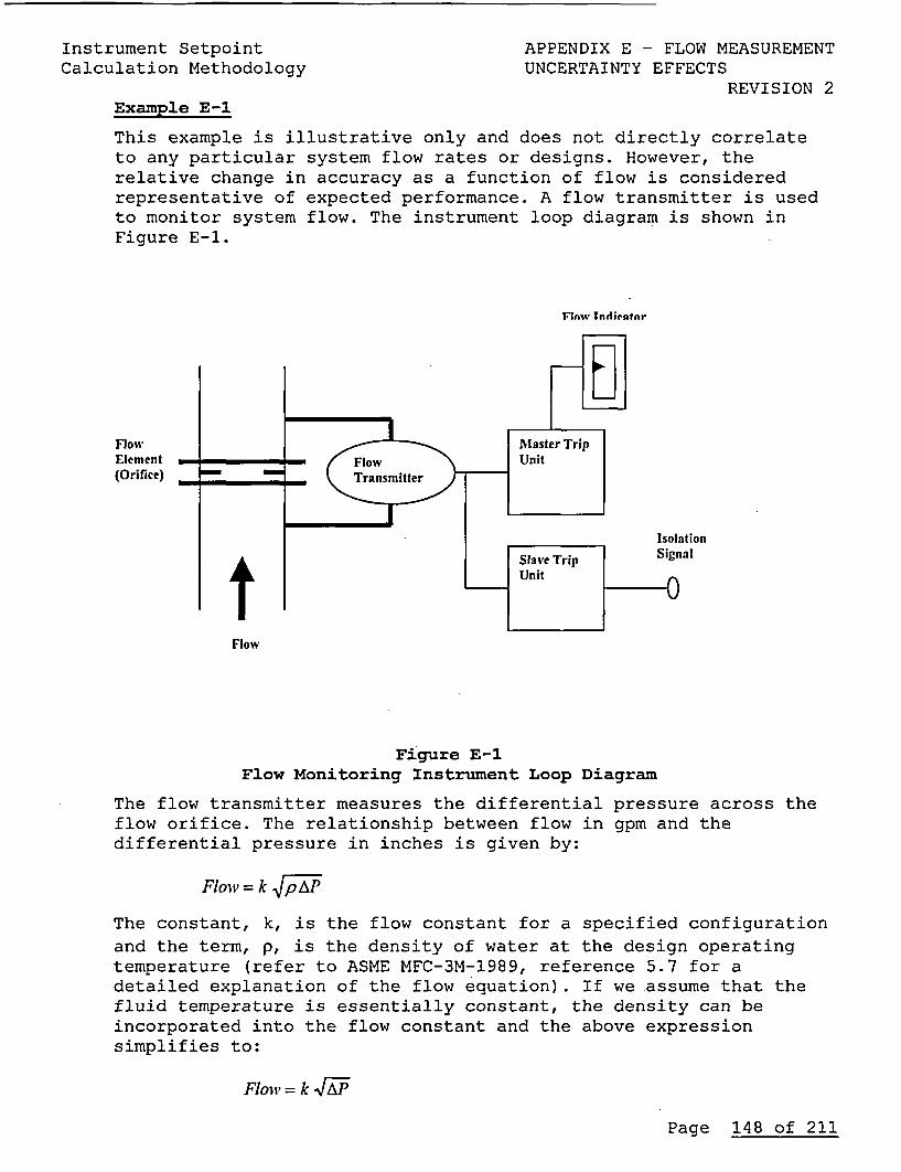
Instrument SetpointCalculation Methodology
APPENDIX E - FLOW MEASUREMENTUNCERTAINTY EFFECTS
REVISION 2Example E-1
This example is illustrative only and does not directly correlateto any particular system flow rates or designs. However, therelative change in accuracy as a function of flow is consideredrepresentative of expected performance. A flow transmitter is usedto monitor system flow. The instrument loop diagram is shown inFigure E-1.
Flnw Indientnr
FlowElement(Orifice)
IsolationSignal
Flow
Figure E-1Flow Monitoring Instrument Loop Diagram
The flow transmitter measures the differential pressure across theflow orifice. The relationship between flow in gpm and thedifferential pressure in inches is given by:
Flow = k 40;iF
The constant, k, is the flow constant for a specified configurationand the term, p, is the density of water at the design operatingtemperature (refer to ASME MFC-3M-1989, reference 5.7 for adetailed explanation of the flow equation). If we assume that thefluid temperature is essentially constant, the density can beincorporated into the flow constant and the above expressionsimplifies to:
Flow = k q
Page 148 of 211
Instrument Setpoint APPENDIX E - FLOW MEASUREMENTCalculation Methodology UNCERTAINTY EFFECTS
REVISION 2For this example and assuming constant fluid temperature, themaximum flow will be given as 1,500 gpm when differential pressureis 100 inches. Therefore, the flow constant is:
k Flow = 1,500 150
Assume that the various manufacturers provided the followingmeasurement uncertainties:
Flow OrificeAccuracy (PEA) - ±1.5%
Flow TransmitterAccuracy (VAT) - ±0-5%Drift (VDT) - ±1.0%Temperature Effects (ATET) - ±0.5%
IndicatorAccuracy (VA,) - ±0.5%Drift (VD,) - ±1.5%
Input ResistorAccuracy (VAR) - ±0.1%
Assume that all of the above uncertainty terms are random andindependent for this example. The transmitter is providing anoutput signal proportional to the differential pressure across theflow orifice.
For this reason, we should first determine the uncertainty in ourdifferential pressure measurement. The flow uncertainty can beestimated by taking the square root of the sum of the squares ofthe individual component uncertainties. The following equation isshown for example only AND does not replace the equations presentedin Section 4.5.4:
Z = (PEA2 + VAT2 + VDT2 + ATET2 + VAI2 + VDI2 + VAR2 ) 1/2
Z 1.552 +0.52+1.02+0.52+0.52+1.52+0.12
= ± 2.5* = ± 2.5 inches AP
Page 149 of 211
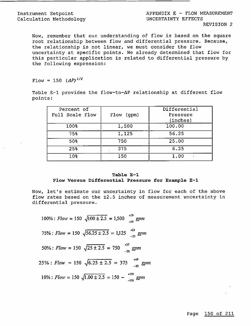
Instrument SetpointCalculation Methodology
APPENDIX E - FLOW MEASUREMENTUNCERTAINTY EFFECTS
REVISION 2
Now, remember that our understanding of flow is based on the squareroot relationship between flow and differential pressure. Because,the relationship is not linear, we must consider the flowuncertainty at specific points. We already determined that flow forthis particular application is related to differential pressure bythe following expression:
Flow = 150 (up) 112
Table E-1 provides thepoints:
flow-to-AP relationship at different flow
Percent of DifferentialFull Scale Flow Flow (gpm) Pressure
(inches)100% 1,500 100.00
75% 1,125 56.25
50% 750 25.00
25% 375 6.25
10% 150 1.00 I
Table E-1Flow Versus Differential Pressure for Example E-1
Now, let's estimate our uncertainty in flow for each of the aboveflow rates based on the ±2.5 inches of measurement uncertainty indifferential pressure.
+19100%: Flow = 150 |f1665±2.5 =1,500 9 gpmn
+2575%: Floii'= 150 156.25 ±2.5 = 1,125 25gprn
50%: Flow = 150 2i5I2.5 = 750 3 gpm-38
+6925% : Flow = 150 46.25 ± 2.5 = 375 85 gpm
-85
.13010%: Flow = 150 jY.002I.5 = 150 - 130 gpm
Page 150 of 211
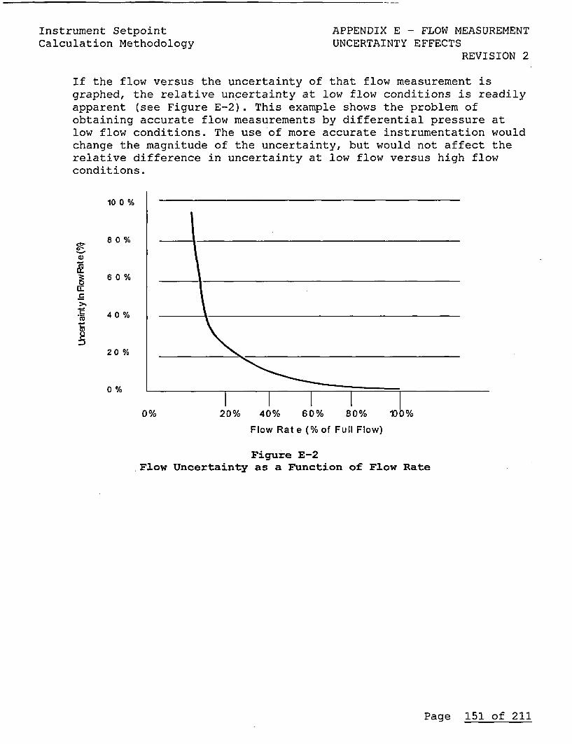
Instrument SetpointCalculation Methodology
APPENDIX E - FLOW MEASUREMENTUNCERTAINTY EFFECTS
REVISION 2
If the flow versus the uncertainty of that flow measurement isgraphed, the relative uncertainty at low flow conditions is readilyapparent (see Figure E-2). This example shows the problem ofobtaining accurate flow measurements by differential pressure atlow flow conditions. The use of more accurate instrumentation wouldchange the magnitude of the uncertainty, but would not affect therelative difference in uncertainty at low flow versus high flowconditions.
cr
C
IAE
10 0 %
8 0 %
6 0 %
40 %
20 %
0 %
Flow Rat e (% of Full Flow)
Figure E-2Flow Uncertainty as a Function of Flow Rate
Page 151 of 211
Instrument Setpoint APPENDIX E - FLOW MEASUREMENTCalculation Methodology UNCERTAINTY EFFECTS
REVISION 2
E.2 Effects of Piping Configuration on Flow Accuracy
Bends, fittings and valves in piping systems cause flow turbulence.This can cause process measurement uncertainties to be induced inflow elements. ASME has published guidance for various types ofinstallation examples to show the minimum acceptableupstream/downstream lengths of straight pipe before and after flowelements. Following this ASME guidance helps reduce the effect ofthis turbulence. The piping arrangement showing locations ofvalves, bends, fittings, etc. can usually be obtained from pipingisometric drawings. Reference 5.7,ASME MFC-3M-1989, states that, ifthe minimum upstream and downstream straight-pipe lengths are met,the resultant flow measurement uncertainty for the pipingconfiguration (not including channel equipment uncertainty) shouldbe assumed to be 0.5%. If the minimum criteria cannot be met,additional uncertainty (at least 0.5%) should be assumed forconservatism based on an evaluation of the piping configuration andfield measurement data, if available.
E.3 Varying Fluid Density Effects on Flow Orifice Accuracy
In many applications, process liquid and gas flows are measuredusing orifice plates and differential pressure transmitters. Themeasurement of concern is either the volumetric flow rate or themass flow rate. Many reference books and standards have beenwritten using a wide variety of terminology to describe themathematics of flow measurement, but in basic form, the governingequations are:
Q = k A (AP /p)1/2
and
W = k A ( (tp) (p) ) 2
where,
Q = Volumetric flow rateW = Mass flow rateA = Cross-sectional area of the pipeAP = Differential pressure measured across the orificep = Fluid densityK = Constant related to the beta ratio, units of measurement,and various correction factors
Page 152 of 211
Instrument Setpoint APPENDIX E - FLOW MEASUREMENTCalculation Methodology UNCERTAINTY EFFECTS
REVISION 2
As shown above, the density of the fluid has a direct influence onthe measured flow rate. Normally, a particular flow-meteringinstallation is calibrated or sized for an assumed normal operatingdensity condition. As long as the actual flowing conditions matchthe assumed density, additional related process errors should notbe present
If the flow-measuring system has been calibrated for the normallow-temperature condition, significant process uncertainties can beinduced under accident conditions when the higher-temperature(lower-density) water is flowing. Of course, the flow measurementcould be automatically compensated for density variations, but thisis not the usual practice except on systems such as steam flowmeasurement.
To examine the effects of changing fluid density conditions, aliquid flow process shall be discussed. For most practicalpurposes, K and A can be considered constant. Actually, temperatureaffects K and A due to thermal expansion of the orifice, but thisis assumed to be constant for this discussion to quantify theeffects of density alone. If the volumetric flow rate, Q, is heldconstant, it is seen that a decrease in density will cause adecrease in differential pressure (AP), causing a measurementuncertainty. This occurs because the differential pressuretransmitter has been calibrated for a particular differentialpressure corresponding to a specific flow rate. A lower AP due to alower fluid density causes the transmitter to indicate a lower flowrate.
Assuming the actual flow remains constant between a base condition(the density at which the instrument is calibrated, P1) and anactual condition (P2), an equality may be written between the baseflow rate (Qj) and actual flow rate (Q2), as shown below:
Q = Q2
or
k A (AP2/p 2) 112 = k A (4Pl/pl)1 2
or
AP 2 /P 2 = AP1/P1 AP2/AP1 = P2/Pl
Page 153 of 211
Instrument Setpoint APPENDIX E - FLOW MEASUREMENTCalculation Methodology UNCERTAINTY EFFECTS
REVISION 2
Density is the inverse of specific volume, SV. Accordingly, theabove expression can be restated in terms of specific volume.
AP2 = SPE
A1I SV2
E.4 Effects of cavitating flows, 1 ratios, and fluid velocity onFlow Orifice Accuracy
There are three elemental considerations to analyze when evaluatingerrors in flow measurement. First is the uncertainty of thecoefficients used to determine the differential pressure of flowrate. This can be termed as flow element error or accuracy.Second is a temperature variation, which occurs during normaloperation, which was discussed in Section E.3 for density effectsbut may also create material property effects such as pipe sizevariations from thermal expansion. The third is flow ratevariation, which will cause the discharge coefficient to varyslightly.
The three primary components of flow element error are:
(1) uncertainty of the discharge coefficient
(2) bore diameter uncertainty and
(3) pipe diameter uncertainty. The diameter ratio is represented
as the bore diameter relative to the pipe diameter or 1 ratioand is given as: diameter ratio = d/D
Where :
d = uncertainty of orifice bore diameterD = uncertainty of upstream pipe diameter
As stated, the discharge coefficient can vary with flow rate andcause the flow coefficient to vary. Flow element installationassumes design condition and therefore a constant flow coefficient(K). Flow Variations decreasing from design flow.will lower theflow element Reynolds number and as Reynolds number falls thedischarge coefficient, C, will rise above the value that existedfor design flow such that the relative error is predicted by:
APA=APD ( 21
APD C
Therefore, flow below design flow induces a small negative biaserror.
Page 154 of 211
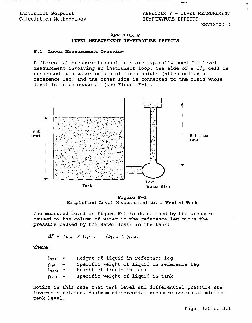
Instrument SetpointCalculation Methodology
APPENDIX F - LEVEL MEASUREMENT
TEMPERATURE EFFECTSREVISION 2
APPENDIX FLEVEL MEASUREMENT TEMPERATURE EFFECTS
F.1 Level Measurement Overview
Differential pressure transmitters are typically used for level
measurement involving an instrument loop. One side of a d/p cell is
connected to a water column of fixed height (often called a
reference leg) and the other side is connected to the fluid whose
level is to be measured (see Figure F-1).
A
TankLevel
LevelTransmit ter
A
ReferenceLevel
V
Tank
Figure F-iSimplified Level Measurement in a Vented Tank
The measured level in Figure F-1 is determined by the pressure
caused by the column of water in the reference leg minus the
pressure caused by the water level in the tank:
AP = (Lref x Yref ) - (Ltank X Ytank)
where,
Lref
Yref =
Ltank =
Ytank =
Height of liquid in reference leg
Specific weight of liquid in reference leg
Height of liquid in tank
specific weight of liquid in tank
Notice in this case that tank level and differential pressure are
inversely related. Maximum differential pressure occurs at minimum
tank level.
Page 155 of 211
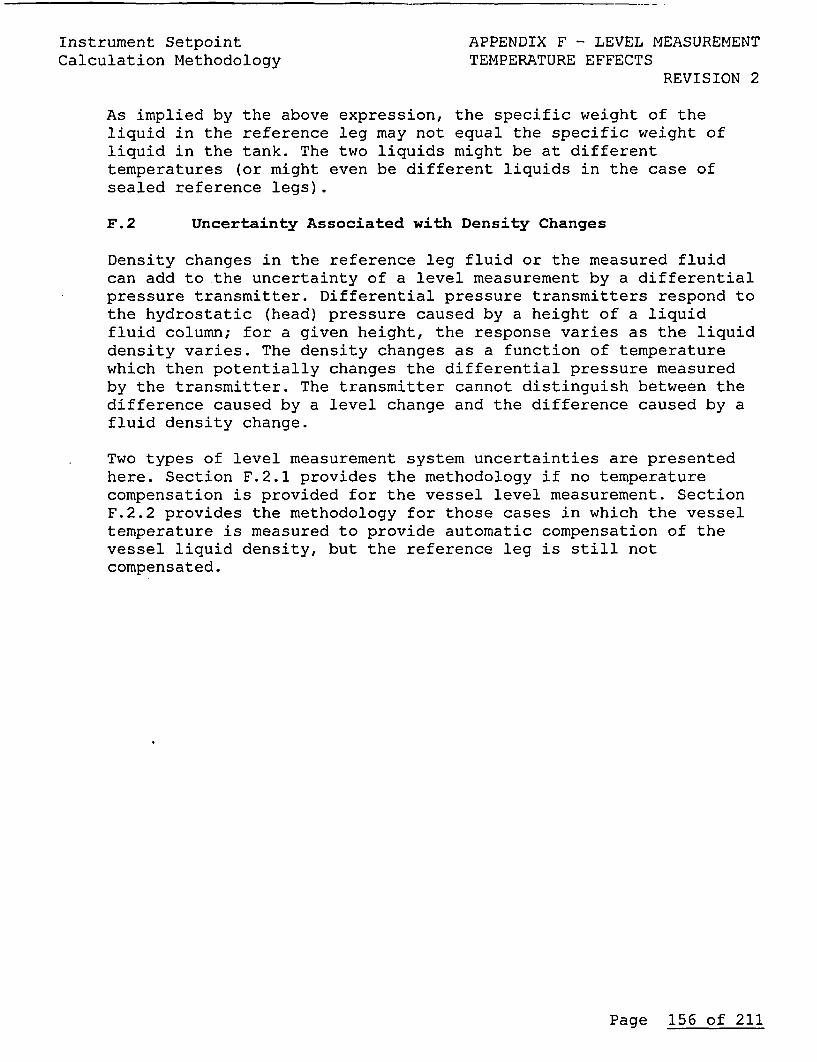
Instrument SetpointCalculation Methodology
APPENDIX F - LEVEL MEASUREMENTTEMPERATURE EFFECTS
REVISION 2
As implied by the above expression, the specific weight of theliquid in the reference leg may not equal the specific weight ofliquid in the tank. The two liquids might be at differenttemperatures (or might even be different liquids in the case ofsealed reference legs).
F.2 Uncertainty Associated with Density Changes
Density changes in the reference leg fluid or the measured fluidcan add to the uncertainty of a level measurement by a differentialpressure transmitter. Differential pressure transmitters respond tothe hydrostatic (head) pressure caused by a height of a liquidfluid column; for a given height, the response varies as the liquiddensity varies. The density changes as a function of temperaturewhich then potentially changes the differential pressure measuredby the transmitter. The transmitter cannot distinguish between thedifference caused by a level change and the difference caused by afluid density change.
Two types of level measurement system uncertainties are presentedhere. Section F.2.1 provides the methodology if no temperaturecompensation is provided for the vessel level measurement. SectionF.2.2 provides the methodology for those cases in which the vesseltemperature is measured to provide automatic compensation of thevessel liquid density, but the reference leg is still notcompensated.
Page 156 of 211
Instrument SetpointCalculation Methodology
APPENDIX F - LEVEL MEASUREMENTTEMPERATURE EFFECTS
REVISION 2
F.2.1 Uncompensated Level Measurement Systems
The methodology developed and described in this section assumesthat vessels are closed and contain a saturated mixture of vaporand water. For this discussion, the reference leg is water-filledand also saturated. Note that the reference leg liquid may well becompressed (subcooled). Figure F-3 shows a closed vessel containinga saturated vapor/water mixture. The symbols used to explain theeffect of density variations are provided immediately below FigureF-3.
H10 0
HO
Vapor l(S G V)
Ta t a t
LevelTank Transmitter
A
HeadReferenceHR
rV
Figure F-3Saturated Liquid/Vapor Level Measurement
Page 157 of 211
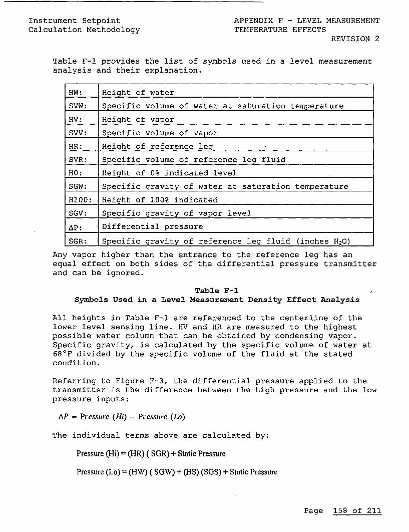
Instrument SetpointCalculation Methodology
APPENDIX F - LEVEL MEASUREMENTTEMPERATURE EFFECTS
REVISION 2
Table F-1 provides the list of symbols used in a level measurementanalysis and their explanation.
HW: Height of water
SVW: Specific volume of water at saturation temperature
HV: Height of vapor
SVV: Specific volume of vapor
HR: Height of reference leg
SVR: Specific volume of reference leg fluid
HO: Height of 0% indicated level
SGW: Specific gravity of water at saturation temperature
H100: Height of 100% indicated
SGV: Specific gravity of vapor level
AP: Differential pressure
SGR: Specific gravity of reference leg fluid (inches H20)
Any vapor higher than the entrance to the reference leg has anequal effect on both sides of the differential pressure transmitterand can be ignored.
Table F-1Symbols Used in a Level Measurement Density Effect Analysis
All heights in Table F-1 are referenced to the centerline of thelower level sensing line. HV and HR are measured to the highestpossible water column that can be obtained by condensing vapor.Specific gravity, is calculated by the specific volume of water at680F divided by the specific volume of the fluid at the statedcondition.
Referring to Figure F-3, the differential pressure applied to thetransmitter is the difference between the high pressure and the lowpressure inputs:
AP = Pressure (Hi) - Pressure (Lo)
The individual terms above are calculated by:
Pressure (Hi) = (HR) ( SGR) + Static Pressure
Pressure (Lo) = (HW) ( SGW) + (HS) (SGS) + Static Pressure
Page 158 of 211
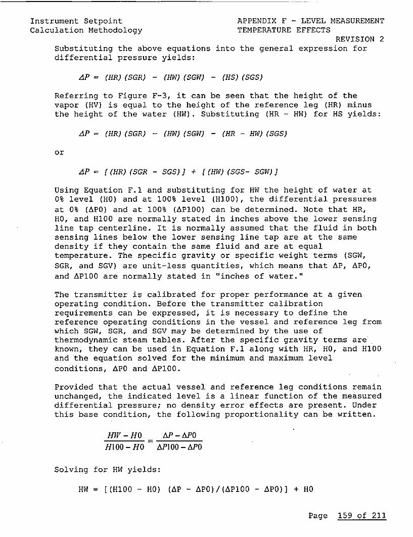
Instrument Setpoint APPENDIX F - LEVEL MEASUREMENTCalculation Methodology TEMPERATURE EFFECTS
REVISION 2Substituting the above equations into the general expression fordifferential pressure yields:
AP = (HR) (SGR) - (HW) (SGW) - (HS) (SGS)
Referring to Figure F-3, it can be seen that the height of thevapor (HV) is equal to the height of the reference leg (HR) minusthe height of the water (HW). Substituting (HR - HW) for HS yields:
AP = (HR) (SGR) - (HW) (SGW) - (HR - HW) (SGS)
or
AP = [ (HR)(SGR - SGS)] + [(HW)(SGS- SGW)]
Using Equation F.1 and substituting for HW the height of water at0% level (HO) and at 100% level (HIOO), the differential pressuresat 0% (APO) and at 100% (AP100) can be determined. Note that HR,HO, and H100 are normally stated in inches above the lower sensingline tap centerline. It is normally assumed that the fluid in bothsensing lines below the lower sensing line tap are at the samedensity if they contain the same fluid and are at equaltemperature. The specific gravity or specific weight terms (SGW,SGR, and SGV) are unit-less quantities, which means that AP, APO,and AP100 are normally stated in "inches of water."
The transmitter is calibrated for proper performance at a givenoperating condition. Before the transmitter calibrationrequirements can be expressed, it is necessary to define thereference operating conditions in the vessel and reference leg fromwhich SGW, SGR, and SGV may be determined by the use ofthermodynamic steam tables. After the specific gravity terms areknown, they can be used in Equation F.1 along with HR, HO, and H100and the equation solved for the minimum and maximum levelconditions, APO and AP100.
Provided that the actual vessel and reference leg conditions remainunchanged, the indicated level is a linear function of the measureddifferential pressure; no density error effects are present. Underthis base condition, the following proportionality can be written.
HIW- HO AP-APO
H100- HO AP100- APO
Solving for HW yields:
HW = [(H100 - HO) (AP - APO)/(AP100 - APO)] + HO
Page 159 of 211
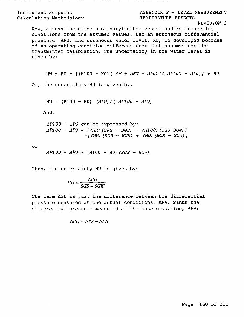
Instrument SetpointCalculation Methodology
APPENDIX F - LEVEL MEASUREMENTTEMPERATURE EFFECTS
REVISION 2Now, assess the effects of varying the vessel and reference legconditions from the assumed values. Let an erroneous differential
pressure, APU, and erroneous water level. HU, be developed becauseof an operating condition different from that assumed for thetransmitter calibration. The uncertainty in the water level isgiven by:
HW ± HU [(H100 - H0) ( AP ± APU - aPO)/( APJOC - APO)] + HO
Or, the uncertainty HU is given by:
HU = (HlO - HO) (aPU)/( APQO0 - APO)
And,
AP100 - APO can be expressed by:AP10 0 - APO [(HR) (SRG - SGS) + (HiCO) (SGS-SGW))
-[(HR) (SGR - SGS) + (HO) (SGS - SGW)]
orAP100 - APO = (H1iO - HO) (SGS - SGW)
Thus, the uncertainty HU is given by:
HU = APUSGS - SGW
The term APU is just the difference between the differentialpressure measured at the actual conditions, APA, minus thedifferential pressure measured at the base condition, APB:
APU = APA-APB
Page 160 of 211
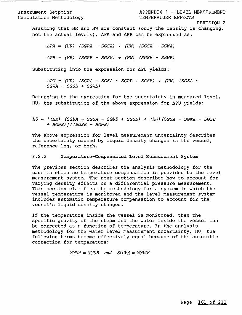
Instrument Setpoint APPENDIX F - LEVEL MEASUREMENTCalculation Methodology TEMPERATURE EFFECTS
REVISION 2Assuming that HR and HW are constant (only the density is changing,not the actual levels), APA and APB can be expressed as:
APA = (HR) (SGRA - SGSA) + (HW) (SGSA - SGWA)
APB = (HR) (SGRB - SGSB) + (HW) (SGSB - SBWB)
Substituting into the expression for APU yields:
APU = (HR) (SGRA - SGSA - SGRB + SGSB) + (HW) (SGSA -SGWA - SGSB + SGWB)
Returning to the expression for the uncertainty in measured level,HU, the substitution of the above expression for APU yields:
HU = [(HR) (SGRA - SGSA - SGRB + SGSB) + (HW)(SGSA - SGWA - SGSB+ SGWB)]/(SGSB - SGWB)
The above expression for level measurement uncertainty describesthe uncertainty caused by liquid density changes in the vessel,reference leg, or both.
F.2.2 Temperature-Compensated Level Measurement System
The previous section describes the analysis methodology for thecase in which no temperature compensation is provided to the levelmeasurement system. The next section describes how to account forvarying density effects on a differential pressure measurement.This section clarifies the methodology for a system in which thevessel temperature is monitored and the level measurement systemincludes automatic temperature compensation to account for thevessel's liquid density changes.
If the temperature inside the vessel is monitored, then thespecific gravity of the steam and the water inside the vessel canbe corrected as a function of temperature. In the analysismethodology for the water level measurement uncertainty, HU, thefollowing terms become effectively equal because of the automaticcorrection for temperature:
SGSA = SGSB and SGIVA = SGIJ'B
Page 161 of 211
Instrument Setpoint APPENDIX F - LEVEL MEASUREMENTCalculation Methodology TEMPERATURE EFFECTS
REVISION 2
In this case, the vessel density effects are eliminated, but notethat the reference leg density changes are not monitored and stillrequire consideration. The uncertainty of the differential pressuremeasurement reduces to:
APU = (HR) (SGRA - SGRB)
The above equation shows that the differential pressure uncertaintybecomes increasingly negative as the actual temperature increasesabove the reference temperature. As the temperature in thereference leg increases above the reference temperature, the fluiddensity decreases, causing a negative APU. Returning to FigureF-3, note that a lower differential pressure means that a higherlevel will be indicated, or a negative APU will cause a positivelevel uncertainty HU. The magnitude of the error can be estimatedby:
HU = (HR) (SGRA - SGRB)/(SGSB - SGWB)
If the transmitter connections were reversed (high pressureconnection reversed with low pressure connection to reverse theAP), the above discussion would still apply, but the uncertaintywould change direction:
APU = (HR) (SGRB - SGRA)
The above equations calculate uncertainties in actual engineeringunits. If desired, the quantities HU and APU can be converted topercent span units by dividing each term by (H100 - HO) or (AP100 -APO), respectively, and multiplying the results by 100%. As
discussed above, the sign (or direction of the uncertainty) for APUdepends on which way the high- and low-pressure sides of thetransmitter are connected to the vessel.
Page 162 of 211
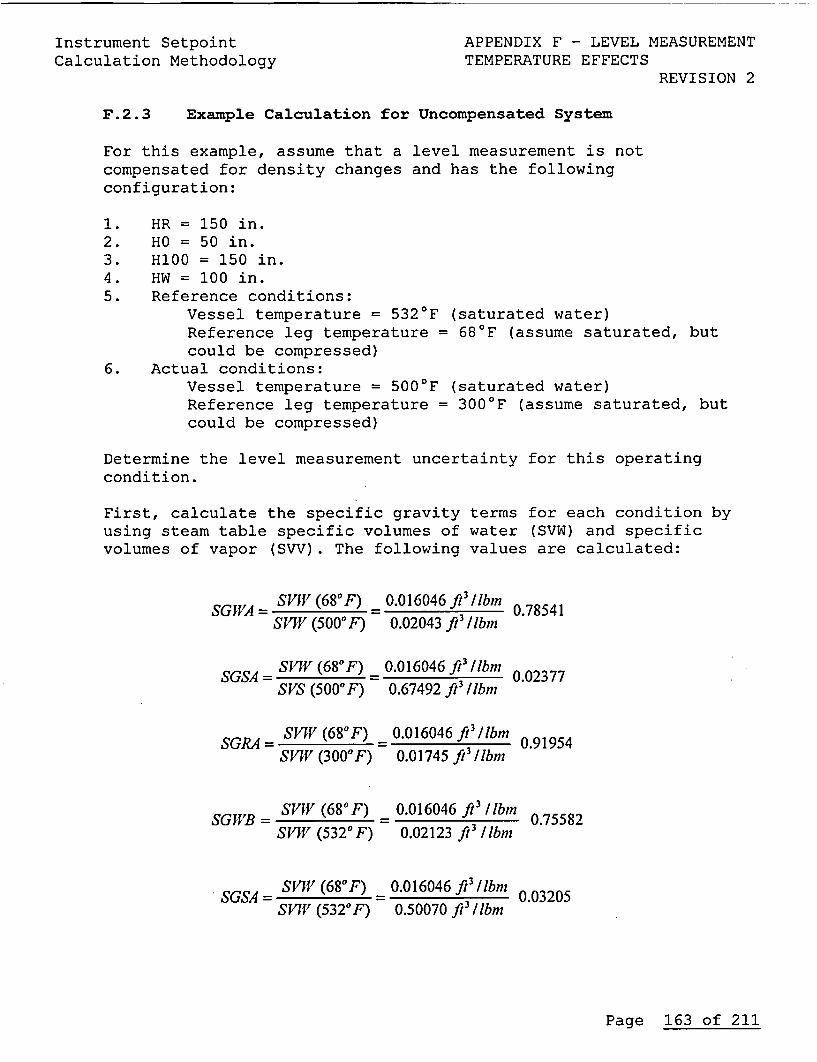
Instrument Setpoint APPENDIX F - LEVEL MEASUREMENTCalculation Methodology TEMPERATURE EFFECTS
REVISION 2
F.2.3 Example Calculation for Uncompensated System
For this example, assume that a level measurement is notcompensated for density changes and has the followingconfiguration:
1. HR = 150 in.2. HO = 50 in.3. H100 = 150 in.4. HW = 100 in.5. Reference conditions:
Vessel temperature = 5320 F (saturated water)Reference leg temperature = 680F (assume saturated, butcould be compressed)
6. Actual conditions:Vessel temperature = 5000F (saturated water)Reference leg temperature = 3000F (assume saturated, butcould be compressed)
Determine the level measurement uncertainty for this operatingcondition.
First, calculate the specific gravity terms for each condition byusing steam table specific volumes of water (SVW) and specificvolumes of vapor (SVV). The following values are calculated:
_ SVW (680F) 0.016046 ft3 llbmSGIVA =- S'(00F) 024 0.78541
SVTV (500°F) 0.02043 fl 3M1m
SGSA SVWV (680F) 0.016046 fM31/bm 0.02377
SVS (5000F) 0.67492 ft3 /Ibrn
SGRA= SVW (680F) 0.016046 ft311bm 0.91954SVW (3000 F) 0.01745 ft3 11bm
_ SVWV (680F) 0.016046 ft3 11bM 7SGJVB - 0.75582
SVWY (532°F) 0.02123 fl 3M1m
SGSA SVI (68°F) 0.016046 ft3 /lbm 0.03205SVW (5320F) 0.50070 ft311bm
Page 163 of 211
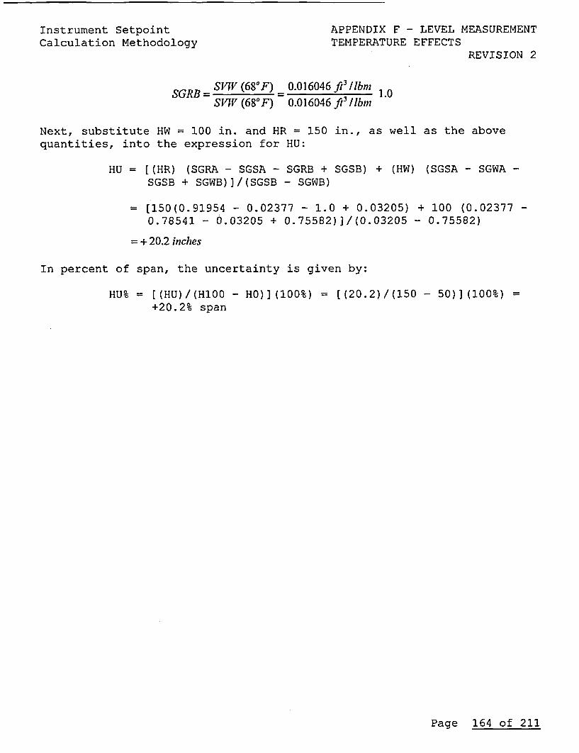
Instrument Setpoint APPENDIX F - LEVEL MEASUREMENTCalculation Methodology TEMPERATURE EFFECTS
REVISION 2
SGRI3 = SVJ (68 F) =0.016046 ft 3 11bm
SVW (680F) 0.016046 ft3 lbm
Next, substitute HW = 100 in. and HR = 150 in., as well as the abovequantities, into the expression for HU:
HU = [(HR) (SGRA - SGSA - SGRB + SGSB) + (HW) (SGSA - SGWA -
SGSB + SGWB)]/(SGSB - SGWB)
= [150(0.91954 - 0.02377 - 1.0 + 0.03205) + 100 (0.02377 -
0.78541 - 0.03205 + 0.75582)]/(0.03205 - 0.75582)
= + 20.2 inches
In percent of span, the uncertainty is given by:
HU% = [(HU)/(H100 - HO)](100%) = [(20.2)/(150 - 50)](100%) =
+20.2% span
Page 164 of 211
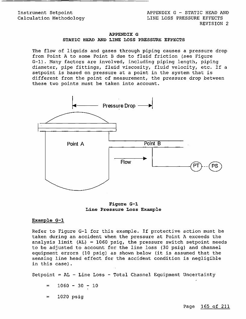
Instrument SetpointCalculation Methodology
APPENDIX G - STATIC HEAD ANDLINE LOSS PRESSURE EFFECTS
REVISION 2
APPENDIX GSTATIC HEAD AND LINE LOSS PRESSURE EFFECTS
The flow of liquids and gases through piping causes a pressure dropfrom Point A to some Point B due to fluid friction (see FigureG-1). Many factors are involved, including piping length, pipingdiameter, pipe fittings, fluid viscosity, fluid velocity, etc. If asetpoint is based on pressure at a point in the system that isdifferent from the point of measurement, the pressure drop betweenthese two points must be taken into account.
[4 Pressure Drop
Point A Point B
Flow a
Figure G-1Line Pressure Loss Example
Example G-1
Refer to Figure G-1 for this example. If protective action must betaken during an accident when the pressure at Point A exceeds theanalysis limit (AL) = 1060 psig, the pressure switch setpoint needsto be adjusted to account for the line loss (30 psig) and channelequipment errors (10 psig) as shown below (it is assumed that thesensing line head effect for the accident condition is negligiblein this case).
Setpoint = AL - Line Loss - Total Channel Equipment Uncertainty
= 1060 -30 -10
- 1020 psig
Page 165 of 211
Instrument Setpoint APPENDIX G - STATIC HEAD ANDCalculation Methodology LINE LOSS PRESSURE EFFECTS
REVISION 2
Note that if the line loss had been neglected and the setpointadjusted to the analysis limit minus equipment error (1050 psig),the resultant setpoint would be non-conservative. In other words,when the trip occurred, the pressure at Point A could be equal to1050 + 30 = 1080 psig, which non-conservatively exceeds theanalysis limit
Example G-2
If the pipe had dropped down vertically to Point B, the resultwould be a head effect plus line loss example. Assume the headpressure exerted by the column of water in the vertical section ofpiping is 5 psig and that the line loss of Point A to Point B isstill equal to 30 psig. Also, assume that the pressure at Point Ais not to drop below 1,500 psig without trip action. For thisexample, the setpoint is calculated as follows:
Setpoint = AL + Head + total Channel Equipment Uncertainty
= 1,500 + 5 + 10 = 1,565 psi
In this case, the 30 psig line loss was neglected for conservatism.
Note that the head effect/line loss errors are bias terms, unlessthey can be calibrated out in the transmitter, in which case thiseffect can be removed from the channel uncertainty calculation.CPS C&I department typically calibrates the effects of head outduring transmitter calibration testing, this must be verified foreach channel during analysis. If head effects are included in thechannel uncertainty calculation, the effect must be added orsubtracted from the analytical limit, depending on the particularcircumstances, to ensure that protective action occurs beforeexceeding the analytical limit.
Page 166 of 211
Instrument Setpoint APPENDIX H - MEASURING AND TESTCalculation Methodology EQUIPMENT UNCERTAINTY
REVISION 2APPENDIX H
MEASURING AND TEST EQUIPMENT UNCERTAINTY
M&TE uncertainty is the inaccuracy introduced by the calibrationprocess due to the limitations of the test instruments. M&TEuncertainty includes three principal components: (1) vendoraccuracy of the test equipment, (2) effect of temperature on thetest equipment, and (3) accuracy of the test equipment calibrationprocess. The first two components are included directly in the M&TEuncertainty and the third is assumed to be included in theconservatism of the vendor accuracy of the test equipment.
All (100%) of test equipment is certified to pass the calibrationrequirements, not just 95%, the common confidence level used foruncertainty calculations. Discussion with vendors shows that theactual accuracy of the test equipment is better than the vendorpublished values. Both of these provide conservatism in theaccuracy of the test equipment and, therefore conservatism in theM&TE determination. As discussed in H.1 below the standards used tocalibrate the test equipment are generally rated 4:1 better thanthe equipment being calibrated. For these reasons it is generallyaccepted that the published vendor accuracy of the test equipmentincludes the uncertainty of the calibration standard since vendoraccuracy divided by 4 is negligible in the relation to otheruncertainties. For the purposes of setpoint and uncertaintycalculations, the total M&TE uncertainty for any module should bebased on test equipment, which has been calibrated using 4:1reference standards.
The module calibration also includes an As-Left tolerance (ALT)which can be related to the test equipment uncertainty. Aninstrument does not provide an exact measurement of the trueprocess value; there is always some level of uncertainty or errorin our measurement. The As-Left tolerance is (1) a reflection ofthe best accuracy that we can realistically obtain or (2) theminimum accuracy that we feel is needed to assure that the processis properly controlled.
For example, a pressure transmitter may have vendor accuracy (VA)of +0.1%, but its As-Left tolerance may be allowed to be ±0.5%.Thus, the instrument technician is allowed to leave the instrumentas-is if it is found anywhere within ±0.5% of the calibration checkpoint. Without any other considerations, we would have to concludethat the calibrated condition of the instrument is only accurate to±0.5% rather than the device's VA of ±0.1%. If greater accuracy isneeded, the calibration procedure should be revised for the tighterAs-Left tolerance.
Appendix H provides the details for calculation preparers toconsider when evaluating the M&TE uncertainty for a module.
Page 167 of 211
Instrument Setpoint APPENDIX H - MEASURING AND TESTCalculation Methodology EQUIPMENT UNCERTAINTY
REVISION 2
H.1 General Requirements
The control of measuring and test equipment (M&TE) is governed atCPS, by procedure CPS 1512.01, Reference 5.14. This procedurerequires the M&TE accuracy to be at least a 4:1 ratio, greater thanthe Reference Standards used. In discussion with NSED, loop M&TE isspecified as the statistical combination of all of the pieces ofinput and output M&TE. Instrument and loop calibration procedures,CPS 8801.01 and 8801.02, References 5.15 and 5.16 required the M&TEto be at least as accurate as the device being calibrated (1:1ratio). CPS does have an M&TE calculation (IP-C-0089, Ref. 5.30)supporting both maintenance selection activities and engineeringassumptions used in calculations.
The following discusses specific requirements of this procedure:
1. Reference standards used for calibrating M&TE shall have anuncertainty (error) requirement of not more than 24 of thetolerance of the M&TE equipment being calibrated. A greateruncertainty may be acceptable as limited by "State of theArt."
2. Total SRSS of M&TE accuracy used for calibrating a loop orcomponent shall have an uncertainty (error) requirement of nomore than a 1:1 ratio of the tolerance of the loop orcomponent being calibrated.
3. No measurement and test equipment shall be used if the recorddate for recalibrating the test equipment has been exceeded.
CPS 1512.01, does not address the accuracy of M&TE equipment withrespect to the loop or component being checked for calibration. Theaccuracy of M&TE equipment is addressed by calculation, CPS (IP-C-0089, Reference 5.30). SRSS of M&TE device(s) accuracy uncertaintywill be considered in terms of the VA of the loop or component tobe calibrated.
For the purposes of setpoint and uncertainty calculations, thetotal M&TE uncertainty should be based on CPS Standard Assumption(Section I.11) that a 4:1 ratio exists between M&TE and referencesstandards, thus CSTD = 0. If the test equipment accuracy is notbased on 4:1 reference standards, the required total M&TEuncertainty should be met by using better test equipment forcalibration.
In general, it is desirable to minimize the contribution of M&TE tothe uncertainty of the loop. Every effort should be made to use themost accurate M&TE available during calibration.
Page 168 of 211
Instrument Setpoint APPENDIX H - MEASURING AND TESTCalculation Methodology EQUIPMENT UNCERTAINTY
REVISION 2H.2 Uncertainty Calculations Based on Plant Calibration Practices
The M&TE uncertainty included in an uncertainty calculation isbased on historical practices and the uncertainty assigned to theM&TE by calculation, IP-C-0089, Ref. 5.30. The implicit designassumption is that M&TE used in the future will be equal to orbetter than the M&TE used in the past (due to improvements in Stateof the Art test equipment). In order to ensure this assumption isnot invalidated by future calibrations, review the M&TE specifiedin the applicable C&I procedures. Verify the uncertainty of theM&TE specified (including calibration standards) is bounded by VAused in the calculation as shown in the following sections for eachtype of instrument or configuration.
NOTE: ALT does not have to equal VA. It can be greater or smallerbased on the needs of C&I maintenance.
H.2.1 Loop Component
For all components, the M&TE reference accuracy used forcalibration should be no greater than VA of that component.
The calculation of Calibration uncertainty should include both theinput and output M&TE. M&TE errors are present with the inputsignal provided to the input of the sensor as well as with theinstrumentation used to measure the output of the sensor (seeFigure H-1). The input M&TE is independent from the output M&TE.Additionally, it should include any other affects on the M&TEequipment such as ATE and/or IRE.
Page 169 of 211
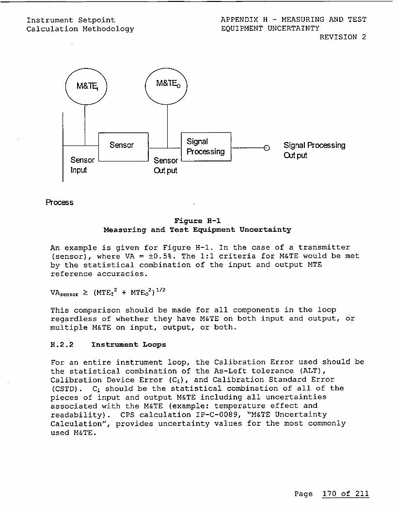
Instrument SetpointCalculation Methodology
APPENDIX H - MEASURING AND TESTEQUIPMENT UNCERTAINTY
REVISION 2
Signal ProcessingOit put
Process
Figure H-1Measuring and Test Equipment Uncertainty
An example is given for Figure H-1. In the case of a transmitter(sensor), where VA = ±0.5%. The 1:1 criteria for M&TE would be metby the statistical combination of the input and output MTEreference accuracies.
VAsensor 2 (MTEI2 + MTEO2) 1/2
This comparison should be made for all components in the loopregardless of whether they have M&TE on both input and output, ormultiple M&TE on input, output, or both.
H.2.2 Instrument Loops
For an entire instrument loop, the Calibration Error used should bethe statistical combination of the As-Left tolerance (ALT),Calibration Device Error (Ci), and Calibration Standard Error(CSTD). Ci should be the statistical combination of all of thepieces of input and output M&TE including all uncertaintiesassociated with the M&TE (example: temperature effect andreadability). CPS calculation IP-C-0089, "M&TE UncertaintyCalculation", provides uncertainty values for the most commonlyused M&TE.
Page 170 of 211
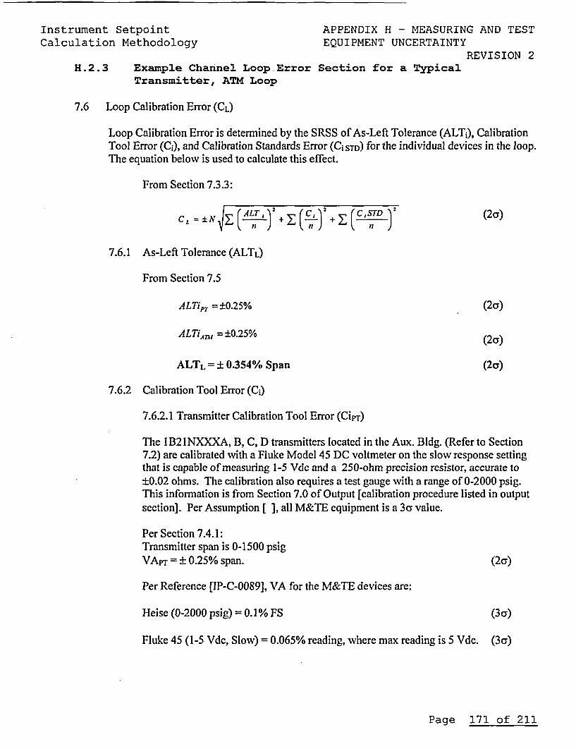
Instrument Setpoint APPENDIX H - MEASURING AND TESTCalculation Methodology EQUIPMENT UNCERTAINTY
REVISION 2H.2.3 Example Channel Loop Error Section for a Typical
Transmitter, ATM Loop
7.6 Loop Calibration Error (CL)
Loop Calibration Error is determined by the SRSS of As-Left Tolerance (ALT;), CalibrationTool Error (Ci), and Calibration Standards Error (C; sTD) for the individual devices in the loop.The equation below is used to calculate this effect.
From Section 7.3.3:
CL=N j (ALT, 2 2( C ) + 2 (2a)
7.6.1 As-Left Tolerance (ALTL)
From Section 7.5
ALTipT = ±0.25% (2a)
ALTiAn,, = ±0.25% (2a)
ALTL = ±0.354% Span (2a)
7.6.2 Calibration Tool Error (C;)
7.6.2.1 Transmitter Calibration Tool Error (Cipr)
The IB2INXXXA, B, C, D transmitters located in the Aux. Bldg. (Refer to Section7.2) are calibrated with a Fluke Model 45 DC voltmeter on the slow response settingthat is capable of measuring 1-5 Vdc and a 250-ohm precision resistor, accurate to±0.02 ohms. The calibration also requires a test gauge with a range of 0-2000 psig.This information is from Section 7.0 of Output [calibration procedure listed in outputsection]. Per Assumption [ ], all M&TE equipment is a 3a value.
Per Section 7.4.1:Transmitter span is 0-1500 psigVApr = ± 0.25% span. (2a)
Per Reference [IP-C-0089], VA for the M&TE devices are:
Heise (0-2000 psig) = 0. 1% FS (3a)
Fluke 45 (1-5 Vdc, Slow) = 0.065% reading, where max reading is 5 Vdc. (3a)
Page 171 of 211
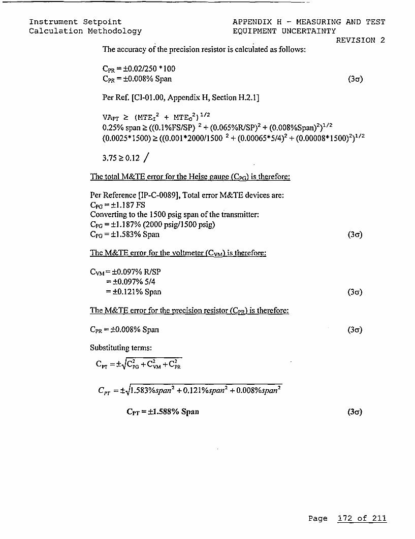
Instrument Setpoint APPENDIX H - MEASURING AND TESTCalculation Methodology EQUIPMENT UNCERTAINTY
REVISION 2The accuracy of the precision resistor is calculated as follows:
CPR = ±0.02/250 * 100CPR = ±0.008% Span (3 c)
Per Ref. [CI-01.00, Appendix H, Section H.2.1]
VAPT 2 (MTE1 2 + MTEo2) 1/2
0.25% span 2 ((0.1%FS/SP) 2 + (0.065%R/SP) 2 + (0.008%Span) 2 )1/2(0.0025* 1500) 2 ((0.001 *2000/1500 2 + (0.00065*5/4)2 + (0.00008* 1500)2)1/2
3.75 2 0.12 /
The total M&TE error for the Heise gauge (Cp6) is therefore:
Per Reference [IP-C-0089], Total error M&TE devices are:CpG = ±1.1 87 FSConverting to the 1500 psig span of the transmitter:CPG = ±1.187% (2000 psig/1500 psig)CPG=±1.583% Span (3c)
The M&TE error for the voltmeter (CvM) is therefore:
CVm = ±0.097% R/SP= ±0.097% 5/4= ±0.121% Span (3a)
The M&TE error for the precision resistor (CPR) is therefore:
CPR = ±0.008% Span (3c)
Substituting terms:
CPT = P + G+ CVC M + CPR
CPT = ± j1.583%span2 + 0.121%span2 + 0.008%span2
CPT= ±l.588% Span (3a)
Page 172 of 211
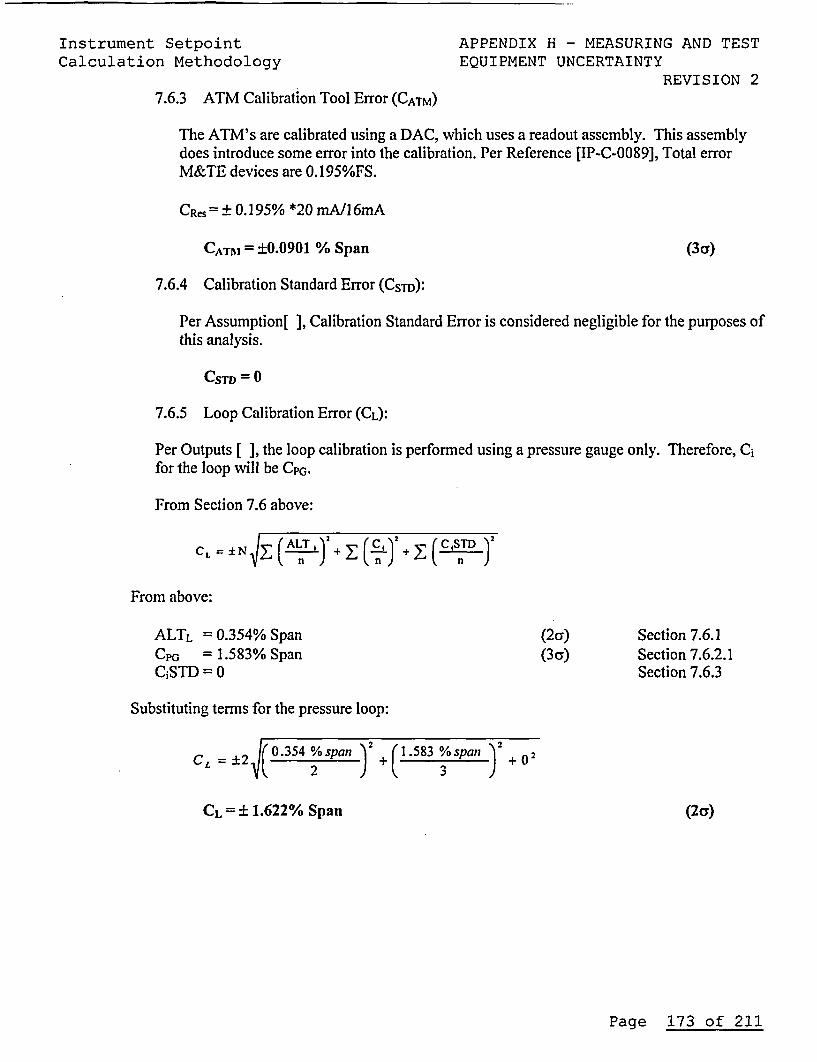
Instrument SetpointCalculation Methodology
APPENDIX H - MEASURING AND TESTEQUIPMENT UNCERTAINTY
REVISION 27.6.3 ATM Calibration Tool Error (CATM)
The ATM's are calibrated using a DAC, which uses a readout assembly. This assemblydoes introduce some error into the calibration. Per Reference [IP-C-0089], Total errorM&TE devices are 0.195%FS.
CReS= ± 0.195% *20 mA/1 6mA
CATAI = ±0.0901 % Span (3a)
7.6.4 Calibration Standard Error (CsTD):
Per Assumption[ ], Calibration Standard Error is considered negligible for the purposes ofthis analysis.
CSTD = 0
7.6.5 Loop Calibration Error (CL):
Per Outputs [ ], the loop calibration is performed using a pressure gauge only. Therefore, C;for the loop will be CPG.
From Section 7.6 above:
A| (ALT.')2 2 CSTD )2CFr=±N above:E
From above:
ALTL = 0.354% SpanCpu = 1.583% SpanCiSTD = 0
(2a)(3cy)
Section 7.6.1Section 7.6.2.1Section 7.6.3
Substituting terms for the pressure loop:
CL = ± 2 (O.354 %span ) 2 +(1.583 %spa? )2 +02
CL = ± 1.62 2 % Span (2(S)
Page 173 of 211
Instrument Setpoint APPENDIX H - MEASURING AND TESTCalculation Methodology EQUIPMENT UNCERTAINTY
REVISION 2H.2.4 Special Considerations
CL is used in the development of AFTL, which is used to calculatedNTSP. In order to preserve an existing setpoint, CL can be reducedas follows:
1. Reduce the M&TE temperature uncertainty by reducing thetemperature band from maximum (Bldg Temp. Band) to a lowerRoom Temp. Band for the location of the component. This willrequire calculating new M&TE uncertainty values consistentwith calculation IP-C-0089.
Discussion and agreement with C&I Maintenance is required for thebelow options, but these may be considered as well;
2. Specify a more accurate M&TE, such as digital heise, which aretemperature compensated. Also, there are some regular heisegauges, which are temperature compensated.
3. Reduce or change the range specified for M&TE. For theexample above, specify a 1500 psig Heise (if it exists).However, the upper Cardinal Point(typically 100% span)used inthe calibration procedure will have to be reduced such thatthe range of the M&TE is not exceeded when allowing for AsFound and As Left calibration tolerances.
Page 174 of 211
Instrument Setpoint APPENDIX I - NEGLIGIBLE UNCERTAINTIESCalculation Methodology /CPS STANDARD ASSUMPTIONS
REVISION 2
APPENDIX INEGLIGIBLE UNCERTAINTIES / CPS STANDARD ASSUMPTIONS
The uncertainties listed and discussed in sections I.1 through I.6below. The CPS Standard Assumptions are listed in I.11. Personnelperforming an uncertainty calculation must evaluate the calculationwith respect to this Appendix to verify that any specialcircumstances or unusual configurations do not invalidate any ofthese negligible uncertainties or CPS Standard Assumptions.
1.1 Normal Radiation Effects
DC-ME-09-CP, Ref. 5.36, defines the normal and harsh environmentsfor areas within the plant. There is not a substantial increase inradiation during normal operating conditions. In these areas,radiation changes during normal operation do not exist and/or areminimal, with no impact to vendor equipment. Normal radiationinduced errors shall be incorporated when provided by themanufacturer. Otherwise, it is assumed that any accumulativeeffects of <104 RAD TID radiation are calibrated out on a periodicbasis. For these reasons, the uncertainty introduced by anyradiation effect during normal operation is assumed to benegligible.
I.2 Humidity Effects
Most manufacturers' literature and technical manuals do not addressthe effect of humidity (10% RH to 95% RH) on their equipment. Theuncertainty introduced by humidity changes during normal operationis assumed to be negligible unless the manufacturer specificallydiscusses humidity effects in the technical manual. The effects ofhumidity changes are assumed to be calibrated out on a periodicbasis. A condensing environment is considered an abnormal eventthat would require equipment maintenance. A humidity below 10% isconsidered to occur very infrequently.
I.3 Seismic/Vibration Effects
The effects of normal vibration (or a minor seismic event that doesnot cause an unusual event) on a component are assumed to becalibrated out on a periodic basis. As such, the uncertaintyassociated with this effect is assumed to be negligible. Abnormalvibrations, e.g., levels that produce noticeable effects onequipment, are considered abnormal events that require maintenanceor equipment modification.
Page 175 of 211
Instrument Setpoint APPENDIX I - NEGLIGIBLE UNCERTAINTIESCalculation Methodology /CPS STANDARD ASSUMPTIONS
REVISION 21.4 Normal Insulation Resistance Effects
The uncertainties associated with insulation resistance are assumedto be negligible during normal plant operating (non-accident)conditions. Typical insulation resistances are greater than 1,000megohm. As an example, assume that the total IR is only 10 megohmand assume minimum instrument loop loading. Using the methodologyprovided in Appendix D, the expected uncertainty attributable to IRis given by:
(48 - (0.004)(250))/((10x106)(0.016)) = 0.03%
As can be seen, the IR can be considered negligible as long as theenvironment remains mild.
1.5 Lead Wire Effects
Since the resistance of a wire is equal to the resistivity timesthe length divided by the cross-sectional area, it is assumed thatthe very small differences in wire lengths between components donot contribute to any significant resistance differences betweenwires. The uncertainty associated with these insignificantresistance variations is assumed to be negligible.
If a system design includes lead wire effects that must beconsidered as a component of uncertainty, the requirement must beincluded in the design basis. The general design standard is toeliminate lead wire effects as a concern both in equipment designand installation. Failure to do so is a design fault that should becorrected. Unless specifically identified to the contrary, leadwire effects are to be assumed to be negligible. An exception tothis is thermocouples and RTDs. These cases require individualevaluation of lead wire effects.
1.6 Calibration Temperature Effects
Calibration temperature is not recorded at CPS, however, thetemperature at which an instrument is calibrated is within thenormal operating range of the instrument and generally reasonablyclose to one another between calibrations. Although, the ambienttemperature effects cannot be determined, they are consideredsmall. Therefore, the uncertainty associated with the temperaturevariations during calibration is assumed to be included within theinstrument drift errors. Note that this applies only to temperaturechanges for calibration. Temperature effects over the expectedrange of equipment operation and M&TE temperature effects must beconsidered.
Page 176 of 211
Instrument Setpoint APPENDIX I - NEGLIGIBLE UNCERTAINTIESCalculation Methodology /CPS STANDARD ASSUMPTIONS
REVISION 2I.7 Atmospheric Pressure Effects
Assuming that the atmospheric pressure might change as much as oneinch of mercury, this equates to approximately 0.5 psi. Becausethis change is small, this effect will be assumed negligible forpressures of 5 psi and larger, unless the pressure transmitter ismeasuring a relatively small pressure.
1.8 Dust Effects
Any uncertainties associated with dust are assumed to becompensated for during normal periodic calibration and are assumedto be negligible.
I.9 RTD Self Heating Errors
To determine a typical RTD self heating error, the followingcomputation is provided:
RTD: Rosemount Model 104 RTDSelf Heating Effect: 0.10C or lessResistance @ 400'C: 249.61 QResistance @ 3800C: 242.58Q2Resistance/0C around 4000C = (249.61 - 242.58)/20
= 0.35 Q/0 CSelf Heating Error = 0.1 0C x 0.35 Q/ 0C = 0.035 Q
At 4000C = 0.035/249.61 = 0.014%
The above results show that the RTD self heating error can beassumed to be negligible.
1.10 Digital Signal Processing
An accuracy of 0.1% of full scale or less is often specified.Additionally, linearity and repeatability are often specified as 1least significant bit (LSB). When this 0.1% uncertainty is comparedto the percent uncertainty for the rest of the instrument loop, itis clear that this uncertainty can be neglected.
Page 177 of 211
Instrument Setpoint APPENDIX I - NEGLIGIBLE UNCERTAINTIESCalculation Methodology /CPS STANDARD ASSUMPTIONS
REVISION 21.11 Assumptions
As defined in Section 2.2, these assumptions are considered to bedefendable and should be used in Section 2.0 for any new or revisedcalculation, performed under this methodology. All standardassumptions shall be listed first without modification, except forwhere an assumption points to another assumption, which may not bethe same number as listed (see assumptions 2.10 & 2.11 below). TheSetpoint Program Coordinator may provide corrections and/or newstandard assumptions that may have not been incorporated into thelatest revision of CI-01.00. It may be necessary to modify some ofthe CPS Standard Assumptions listed below during the development orrevision of calculations. The preparer and reviewer of acalculation must ensure the assumptions used are valid andapplicable to their calculation.
2.1 Published instrument vendor specifications are considered tobe 2a values unless specific information is available toindicate otherwise
2.2 Temperature, humidity, power supply, and ambient pressureerrors have been incorporated when provided by themanufacturer. Otherwise, these errors are assumed to beincluded in the manufacturer's accuracy or repeatabilityspecifications
2.3 Changes in ambient humidity are assumed to have a negligibleeffect on the uncertainty of the instruments used in theseloops.
2.4 Normal radiation induced errors have been incorporated whenprovided by the manufacturer. Otherwise, these errors areassumed to be small and capable of being adjusted out eachtime the instrument is calibrated. Therefore, unlessspecifically provided, normal radiation errors can be assumedto be included within the instrument drift errors.
2.5 If the manufacturers instrument performance data does notspecify Span, Calibrated Span, Upper Range Limit, etc. thecalculation will assume URL because it will result in the mostconservative estimate of instrument uncertainty. In all casesthe URL is greater than or equal to the calibrated span (CS)and it is conservative to use the URL in calculatinginstrument uncertainties. This is because, by definition, URLis the maximum upper calibrated span limit for the device.
Page 178 of 211
Instrument Setpoint APPENDIX I - NEGLIGIBLE UNCERTAINTIESCalculation Methodology /CPS STANDARD ASSUMPTIONS
REVISION 22.6 This analysis assumes that the instrument power supply
stability (PSS) is within +5% (+1.2 Vdc) of a nominal 24 Vdc.
2.7 The effects of normal vibration (or a minor seismic event thatdoes not cause an unusual event) on a component are assumed tobe calibrated out on a periodic basis. As such, theuncertainty associated with this effect is assumed to benegligible and included within the instrument drift errors.Abnormal vibrations, e.g., levels that produce noticeableeffects on equipment, are considered abnormal events thatrequire maintenance or equipment modification.
2.8 Evaluation of M&TE errors is based on the assumption that thetest equipment listed in Analysis Section 7.0 is used. Use oftest equipment less accurate than that listed will requireevaluation of the effect on calculation results.
2.9 It is assumed that the M&TE listed in Section 7.0 iscalibrated to the required manufacturer's recommendations andwithin the manufacturer's required environmental conditions.Temperature related errors are based on the difference betweenthe Calibration Lab temperature and the worst case temperatureat which the device is used.
2.10 It is assumed that the reference standards used forcalibrating M&TE or Calibration tools shall have uncertaintyrequirements of not more than 4 of the tolerance of theequipment being calibrated. A greater uncertainty may beacceptable as limited by "State of the Art". It is generallyaccepted that the published vendor accuracy of the M&TE orCalibration tool includes the uncertainty of the calibrationstandard M&TE when the 4:1 accuracy standard is satisfied.Hence, Calibration Standard uncertainty is considerednegligible to the overall calibration error term and can beignored. This assumption is based primarily upon inherentM&TE conservatism built into the calculation. Per assumption[2.11], this calculation considers the combined M&TE vendor orreference accuracy used for calibration satisfies 1:1 accuracyratio to the instrument under calibration. This ratio boundsthe upper accuracy limit on Calibration tool equal to theVendor's Accuracy (VA) specification for the device undercalibration. Use of M&TE more accurate than 1:1 isconservative to this assumption and thereby acceptable withoutimpacting the results of this calculation.
Page 179 of 211
Instrument Setpoint APPENDIX I - NEGLIGIBLE UNCERTAINTIESCalculation Methodology /CPS STANDARD ASSUMPTIONS
REVISION 22.11 It is assumed that when M&TE is not specified uniquely in a
controlling calibration procedure (e.g., SurveillanceProcedure or Preventive Maintenance Procedure), the combinedM&TE vendor or reference accuracy used for calibrationsatisfies a 1:1 accuracy ratio to the instrument undercalibration. This accuracy ratio establishes the limit onselected M&TE equal to the Vendor's Accuracy (VA) requirement.Further, M&TE uncertainty assumed per this discussion, isconsidered a 3a value regardless of the confidence associatedwith the related VA term.
2.12 The effects of EMI and RFI are considered negligible for panelmounted meters in administratively controlled EMI/RFIenvironments, unless a specific uncertainty term is providedby the vendor.
2.13 If the instrument vendor provides no drift information andthere is no clear basis for assuming drift is zero, it may beconservatively assumed that the drift over the entirecalibration period equals Vendor Accuracy (i.e., VD = VA 2a).
2.14 Data from comparable but different instruments may be usedwhen vendor specification is not available or is lacking.This comparison should evaluate like applications in likeenvironment with the instrument analyzed consistent for form,fit, and function.
Page 180 of 211
Instrument Setpoint APPENDIX J - DIGITAL SIGNALCalculation Methodology PROCESSING UNCERTAINTIES
REVISION 2
APPENDIX JDIGITAL SIGNAL PROCESSING UNCERTAINTIES
This Appendix presents a discussion on digital signal processingand the uncertainties involved with respect to determininginstrument channel setpoints for a digital system. This Appendixassumes that a digital signal processing system exists thatreceives an analog signal and provides either a digital or analogoutput. In many respects, the digital processor is treated as ablack box; therefore, the discussion that follows is applicable tomany different types of digital processors.
The digital processor is programmed to perform a controlledalgorithm. Basic functions performed are addition, subtraction,multiplication and division, as well as data storage. The digitalprocessor is the most likely component to introduce rounding andtruncation errors.
In general, an analog signal is received by the digital processor,filtered, digitized, manipulated, converted back into analog form,filtered again and sent out. The analog input signal is firstprocessed by a filter to reduce aliasing noise introduced by thesignal frequencies that are high relative to the sampling rate. Thefiltered signal is sampled at a fixed rate and the amplitude of thesignal held long enough to permit conversion to a digital word. Thedigital words are manipulated by the processor based on thecontrolled algorithm. The manipulated digital words are convertedback to analog form, and the analog output signal is smoothed by areconstruction filter to remove high-frequency components.
Several factors affect the quality of the representation of analogsignals by digitized signals. The sampling rate affects aliasingnoise, the sampling pulse width affects analog reconstructionnoise, the sampling stability affects jitter noise and thedigitizing accuracy affects the quantization noise.
J.1 Sampling Rate Uncertainty
If the sampling rate is higher than twice the analog signalbandwidth, then the sampled signal is a good representation of theanalog input signal and contains all the significant information.If the analog signal contains frequencies that are too high withrespect to the sampling rate, aliasing uncertainty will beintroduced. Anti-aliasing band limiting filters can be used tominimize the aliasing uncertainty or else it should be accountedfor in setpoint calculations.
Page 181 of 211
Instrument Setpoint APPENDIX J - DIGITAL SIGNALCalculation Methodology PROCESSING UNCERTAINTIES
REVISION 2J.2 Signal Reconstruction Uncertainty
Some information is lost when the digitized signal is sampled andheld for conversion back to analog form after digital manipulation.This uncertainty is typically linear and about ±+ Least SignificantBit (LSB).
J.3 Jitter Uncertainty
The samples of the input signal are taken at periodic intervals. Ifthe sampling periods are not stable, an uncertainty correspondingto the rate of change of the sampled signal will be introduced. Thejitter uncertainty is insignificant if the clock is crystalcontrolled, which it is in the majority of cases.
J.4 Digitizing Uncertainty
When the input signal is sampled, a digital word is generated thatrepresents the amplitude of the signal at that time. The signalvoltage must be divided into a finite number of levels that can bedefined by a digital word n bits long. This word will describe 2ndifferent voltage steps. The signal levels between these steps willgo undetected. The digitizing uncertainty (also known as thequantizing uncertainty) can be expressed in terms of the total meansquare error voltage between the exact and the quantized samples ofthe signal. An inherent digitizing uncertainty of ±+ the leastsignificant bit (LSB) typically exists. The higher the numbers ofbits in the conversion process the smaller the digitizinguncertainty.
J.5 Miscellaneous Uncertainties
Analog-to-digital converters also introduce offset uncertainty,i.e., the first transition may not occur at exactly ±+ LSB. Gainuncertainty is introduced when the difference between the values atwhich the first transition and the last transition occurs is notequal. Linearity uncertainty is introduced when the differencesbetween the transition values are not all equal.
As a rule of thumb, use id LSB for relative uncertainty for theanalog-to-digital conversion. For digital-to-analog conversion, themaximum linearity uncertainty occurs at full scale when all bitsare in saturation. The linearity determines the relative accuracyof the converters. Deviations from linearity, once the convertersare calibrated, is absolute uncertainty. As a rule of thumb, use ±+LSB for absolute uncertainty and ± LSB for linearity uncertainty.
Page 182 of 211
Instrument Setpoint APPENDIX J - DIGITAL SIGNALCalculation Methodology PROCESSING UNCERTAINTIES
REVISION 2J.6 Truncation and Rounding Uncertainties
The effect of truncation or rounding depends on whether fixed-pointor floating-point arithmetic is used and how negative numbers arerepresented. For the sign-and-magnitude one's compliment and two'scompliment methods, the numbers are represented identically. Thelargest truncation error occurs when all bits discarded are one's.
For negative numbers, the effect of truncation depends on whethersign-and-magnitude, two's compliment or one's complimentrepresentation is used. Rounding is used on the magnitude of thenumbers, and uncertainty is independent of the method of negativenumbers representation.
For positive numbers and two's compliment negative numbers, thetruncation uncertainty is estimated by:
_2-6 < ET < 0
For sign-and-magnitude and one's compliment negative numbers, thetruncation uncertainty is estimated by:
0 S ET < 2-
where b is the number of bits to the right of the binary pointafter truncation or rounding.
Estimation for rounding uncertainty is:
(-1/2)(2 -b) < ER < (1/2)(2 -b)
Where b, is the number of bits to the right of the binary pointafter truncation or rounding. Truncation and rounding Effects themantissa in floating point arithmetic. The relative uncertainty ismore important than the absolute uncertainty, i.e., floating-pointerrors are multiplicative.
For floating point arithmetic, the relative uncertainty forrounding is estimated by:
-2.2 b < E • 0
For one's compliment and sign-and-magnitude, truncation uncertaintyis estimated by:
-2.2-b < E • 0, for X <0
0 • E < 2 .2-b, for X >0
Where X is the sign and magnitude value prior to truncation.
Page 183 of 211
Instrument Setpoint APPENDIX K - PROPAGATION OF UNCERTAINTYCalculation Methodology THROUGH SIGNAL CONDITIONING MODULES
REVISION 2
APPENDIX KPROPAGATION OF UNCERTAINTY THROUGH
SIGNAL CONDITIONING MODULES
This Appendix discusses techniques for determining the uncertaintyof a module's output when the uncertainty of the input signal andthe uncertainty associated with the module are known. Using thesetechniques, equations are developed to determine the outputuncertainties for several common types of functional modules.
For brevity, error propagation equations (See Table K-1) will notbe derived for all types of signal-processing modules. Equationsfor only the most important signal-processing functions will bedeveloped; however, the methods discussed -can be applied tofunctions not specifically addressed here. The equations derivedare applicable to all signal conditioners of that type regardlessof the manufacturer.
The techniques presented here are not used to calculate theinaccuracies of individual modules; they are used to calculateuncertainty of the output of a module when the module inaccuracy,input signal uncertainty and module transfer function are known.
This section discusses only two classifications of errors oruncertainties: those, which are random and independent and can becombined statistically, and those, which are biases, which must becombined algebraically. The methods discussed can be used for bothrandom and biased uncertainty components.
It is important to note that the method of calibration or testingmay directly affect the use of the information presented in thissection. If, for example, all modules in the process electronicsfor a particular instrument channel are tested together, they maybe considered one device. The uncertainty associated with theoutput of that device should be equal to or less than theuncertainty calculated by combining all individual modules.
K.1 Error Propagation Equations Using Partial Derivatives andPerturbation Techniques
There are several valid approaches for the derivation of equations,which express the effect of passing an input signal with an errorcomponent through a module that performs a mathematical operationon the signal. The approaches discussed here, which are recommendedfor use in developing error-propagation equations, are based on theuse of partial derivatives or perturbation techniques, i.e.,changing the value of a signal by a small amount and evaluating theeffect of the change on the output. Either technique is acceptableand the results, in most cases, are similar.
Page 184 of 211
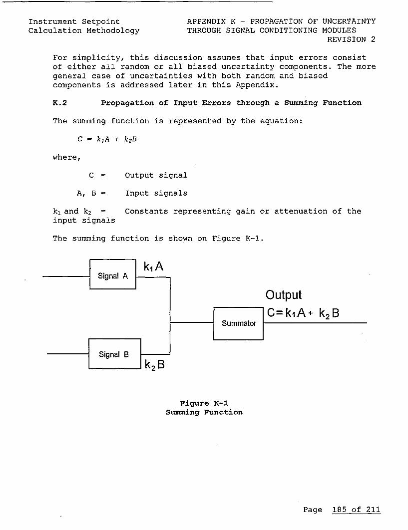
Instrument SetpointCalculation Methodology
APPENDIX K - PROPAGATION OF UNCERTAINTYTHROUGH SIGNAL CONDITIONING MODULES
REVISION 2
For simplicity, this discussion assumes that input errors consistof either all random or all biased uncertainty components. The moregeneral case of uncertainties with both random and biasedcomponents is addressed later in this Appendix.
K.2 Propagation of Input Errors through a Summing Function
The summing function is represented by the equation:
C = k1 A + k 2 B
where,
C =
A, B =
k1 and k2 =
input signals
Output signal
Input signals
Constants representing gain or attenuation of the
The summing function is shown on Figure K-1.
k1A
OutputC=kiA+ k2B
k2B
Figure K-1Summing Function
Page 185 of 211
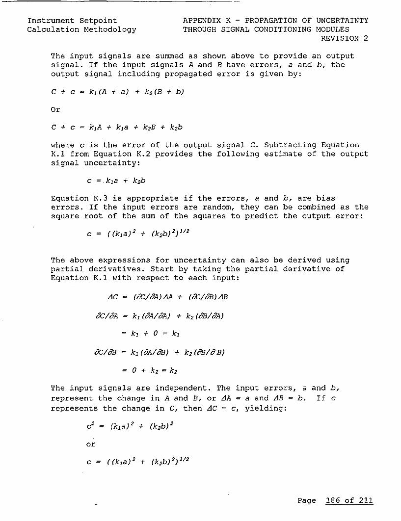
Instrument SetpointCalculation Methodology
APPENDIX K - PROPAGATION OF UNCERTAINTYTHROUGH SIGNAL CONDITIONING MODULES
REVISION 2
The input signals are summed as shown above to provide an outputsignal. If the input signals A and B have errors, a and b, theoutput signal including propagated error is given by:
C + c = k1 (A + a) + k2 (B + b)
Or
C + c = kjA + kja + k 2B + k 2 b
where c is the error of the output signal C. Subtracting EquationK.1 from Equation K.2 provides the following estimate of the outputsignal uncertainty:
c =. kja + k2 b
Equation K.3 is appropriate if the errors, a and b, are biaserrors. If the input errors are random, they can be combined as thesquare root of the sum of the squares to predict the output error:
c = ((kia) 2 +(k2b) 2) 112
The above expressions for uncertainty can also be derived usingpartial derivatives. Start by taking the partial derivative ofEquation K.l with respect to each input:
AC = (X1/dA) aA + (k¼9dB) aB
X1/A = ki (A/19A) + k2 (oB/MA)
= kj + 0 = kj
XlodB = ki (cA/e9B) + k2 (o-B/c9B)
= - + k 2 = k2
The input signals are independent. The input errors, a and b,represent the change in A and B, or AA = a and AB = b. If c
represents the change in C, then AC = c, yielding:
C2 = (kia)2 + (k 2 b) 2
or
c = ((ka) 2 + (k 2 b) 2 ) 2
Page 186 of 211
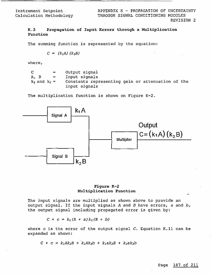
Instrument SetpointCalculation Methodology
APPENDIX K - PROPAGATION OF UNCERTAINTYTHROUGH SIGNAL CONDITIONING MODULES
REVISION 2
K.3 Propagation of Input Errors through a MultiplicationFunction
The summing function is represented by the equation:
C = (k 1 A) (k 2B)
where,
CA, Bk, and k2
Output signalInput signalsConstants representing gain or attenuation of theinput signals
The multiplication function is shown on Figure K-2.
k1A
OutputC= (kiA) (k2 B)
k2B
Figure K-2Multiplication Function
The input signals are multiplied as shown above to provide anoutput signal. If the input signals A and B have errors, a and b,the output signal including propagated error is given by:
C + c = k1 (A + a)k2 (B + b)
where c is the error of the output signal C. Equation K.11 can beexpanded as shown:
C + c = kjAk 2 B + k 1 Ak 2 b + kjak2 B + kjak2 b
Page 187 of 211
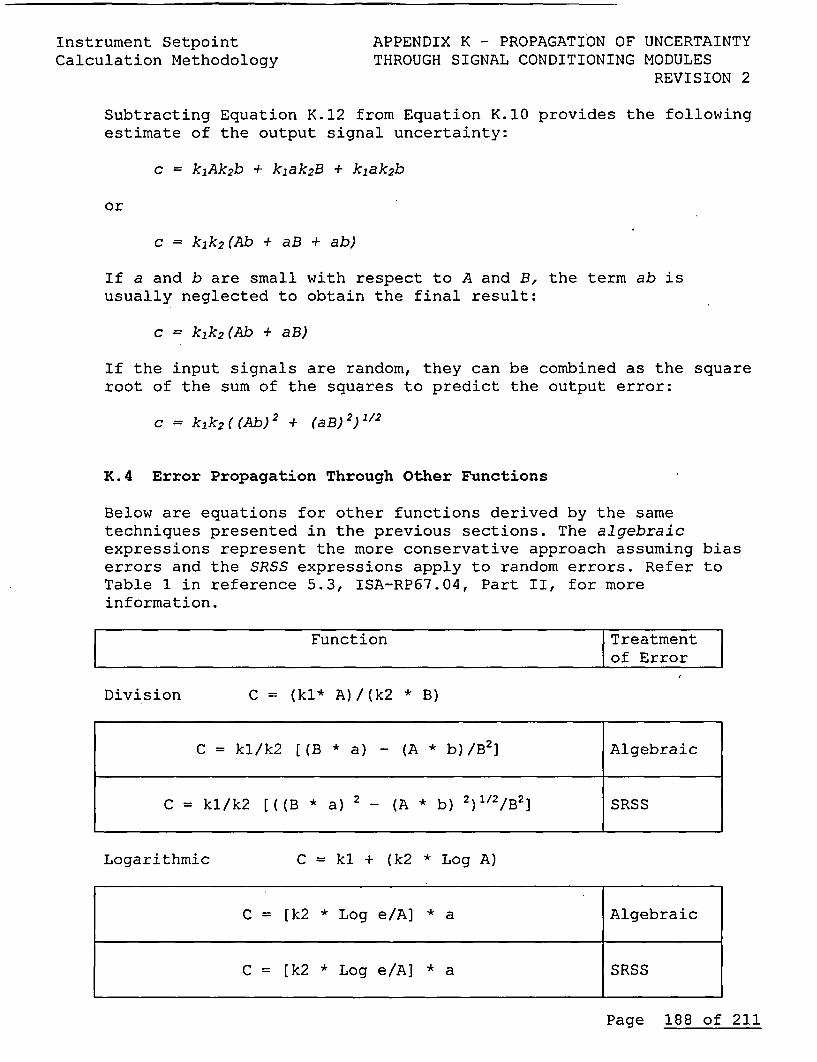
Instrument SetpointCalculation Methodology
APPENDIX K - PROPAGATION OF UNCERTAINTYTHROUGH SIGNAL CONDITIONING MODULES
REVISION 2
Subtracting Equation K.12 from Equation K.10 provides the followingestimate of the output signal uncertainty:
c = kjAk 2 b + klak2 B + kjak2 b
or
c = kjk 2 (Ab + aB + ab)
If a and b are small with respect to A and B, the term ab isusually neglected to obtain the final result:
c = kjk2 (Ab + aB)
If the input signals are random, they can be combined as the squareroot of the sum of the squares to predict the output error:
c = kjk 2 ((Ab) 2 +(aB) 2) 112
K.4 Error Propagation Through Other Functions
Below are equations for other functions derived by the sametechniques presented in the previous sections. The algebraicexpressions represent the more conservative approach assuming biaserrors and the SRSS expressions apply to random errors. Refer toTable 1 in reference 5.3, ISA-RP67.04, Part II, for moreinformation.
Function Treatment|of Error
Division C = (kl* A)/(k2 * B)
C = kl/k2 [(B * a) - (A * b)/B2] Algebraic
C = kl/k2 [((B *a) 2 (A *b) 2)1/2/B 2] SRSS
Logarithmic C kl + (k2 * Log A)
C = [k2 * Log e/A] * a Algebraic
C = [k2 *Log e/A] *a SRSS
Page 188 of 211
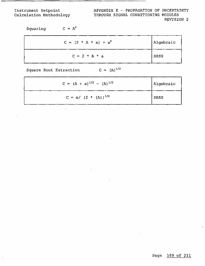
Instrument SetpointCalculation Methodology
APPENDIX K - PROPAGATION OF UNCERTAINTYTHROUGH SIGNAL CONDITIONING MODULES
REVISION 2
Squaring C = A2
C = (2 * A * a) + a2 Algebraic
C = 2 * A * a SRSS
Square Root Extraction C = (A) 1/2
C = (A + a)1 12 _ (A)1/2 Algebraic
C = a/ (2 * (A))1 12 SRSS
Page 189 of 211
Instrument Setpoint APPENDIX L - GRADED APPROACH TOCalculation Methodology UNCERTAINTY ANALYSIS
REVISION 2
APPENDIX LGRADED APPROACH TO UNCERTAINTY ANALYSIS
L.1 Introduction
The methodology presented in this engineering standard is intendedto establish a minimum 95% probability with a high confidence thata setpoint will actuate when required. The methodology is based,in part, on ISA -S67.04, Reference 5.3.
When a calculation is prepared in accordance with this engineeringstandard, it will accomplish a rigorous review of the instrumentloop layout and design. Each element of uncertainty will beevaluated in detail and the estimated loop uncertainty justified atlength. The setpoint will be carefully established with respect tothe process analytical limit and channel uncertainty. Acalculation prepared with this engineering standard will becomprehensive and can typically take an engineer at least two weeksto prepare. This level of effort is justified for thosecalculations involving reactor safety and integrity.
The importance of the various types of safety-related setpointsdiffer, and as such it may be appropriate to apply differentsetpoint determinations requirements. As described in Reference5.3, for automatic setpoints that has a significant importance tosafety. For example, those required by the plant safety analysesand directly related to Reactor Protection System, Emergency Core-Cooling Systems, Containment Isolation, and Containment HeatRemoval, a stringent setpoint methodology should consider allsources of instrument error. However, for setpoints that may nothave the same level of stringent requirements, for example, thosethat are not credited in the safety analyses or that do not havelimiting values, the setpoint determination methodology could beless rigorous. The level of detail should be commensurate withthe importance of the application.
Multiple setpoint methodologies for engineering calculations havebeen attributed-to programmatic setpoint errors at other powerstations. These stations have incorporated corrective actions thatimplement setpoint and loop uncertainty analysis that are balancedwith the importance or significance of the related plant systemsafety function. This approach is acceptable and is consistentwith a draft recommended practice by Instrument Society of America(ISA) standards, (ISA dTR 67.04.09, Graded Approaches to SetpointDetermination, Draft Technical Report, 1994 and the subsequentversion Draft 4, May, 2000). This Appendix provides guidanceregarding how to satisfy the needs for proper setpoint controlwhile allowing for simpler approaches for less criticalapplications.
Page 190 of 211
Instrument Setpoint APPENDIX L - GRADED APPROACH TOCalculation Methodology UNCERTAINTY ANALYSIS
REVISION 2The CPS setpoint methodology will establish the basis of a gradedsetpoint program by grouping the instrument loops according totheir safety significance. The graded approach to setpointdetermination provides the maximum available tolerance to optimizethe safety and reliability of the plant.
Graded approaches are based on fact that all the rigor andconservatism established in RP67.04-1994, Part II may not bewarranted for all setpoints in a nuclear power plant. Per RP67.04-1994, a nuclear plant licensee may establish a multilevelclassification scheme by documenting the rationale used toestablish the classification. Implementation of a graded approachto setpoints requires the users to identify how criticallyimportant each setpoint is. For example, setpoints for RPS andESFAS are to be maintained with a high degree of conservatism and ahigh level of confidence. Setpoints for Reg. Guide 1.97, Type Cvariables for post accident monitoring do not require the samelevel of confidence. Therefore, a graded approach, withclassification for setpoints, will help proper maintenance ofsafety grade nuclear instrumentation without compromising the safeand reliable operation of the plant.
L.2 GRADED CLASSIFICATIONS
CPS Setpoint Control distinguishes between applications byproviding the following classifications of setpoint categories interms of safety significance. For example, Setpoint Category 1instrument loops are deemed safety significant and calculations forthis class of instruments would require full rigor and conservatismestablished in RP67.04-1994, Part II for safety related setpoints.The Setpoint Category Tables are presented in order of descendingsafety significance and therefore, calculation rigor.
Page 191 of 211
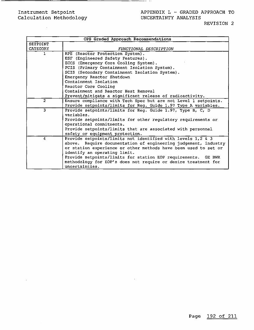
Instrument SetpointCalculation Methodology
APPENDIX L - GRADED APPROACH TOUNCERTAINTY ANALYSIS
REVISION 2
CPS Graded Approach Recommendations
SETPOINTCATEGORY FUNCTIONAL DESCRIPTION
1 RPS (Reactor Protection System).ESF (Engineered Safety Features).ECCS (Emergency Core Cooling System).PCIS (Primary Containment Isolation System).SCIS (Secondary Containment Isolation System).Emergency Reactor ShutdownContainment IsolationReactor Core CoolingContainment and Reactor Heat RemovalPrevent/mitigate a significant release of radioactivity.
2 Ensure compliance with Tech Spec but are not Level 1 setpoints.Provide setpoints/limits for Reg. Guide 1.97 Type A variables.
3 Provide setpoints/limits for Reg. Guide 1.97, Type B, C, Dvariables.Provide setpoints/limits for other regulatory requirements oroperational commitments.Provide setpoints/limits that are associated with personnelsafety or equipment protection.
4 Provide setpoints/limits not identified with levels 1,2 & 3above. Require documentation of engineering judgement, industryor station experience or other methods have been used to set oridentify an operating limit.Provide setpoints/limits for station EOP requirements. GE BWRmethodology for EOP's does not require or desire treatment foruncertainties.
Page 192 of 211
Instrument SetpointCalculation Methodology
APPENDIX L - GRADED APPROACH TOUNCERTAINTY ANALYSIS
REVISION 2
The following guidelines should be followed with regard to thelevel of rigor required for a setpoint determination.
Cat. 1 and 2:
Cat 3:
Cat 4:
A Calculation in accordance with NSED Procedure E.1is required. Setpoints must be prepared inaccordance with this standard and must account forall known sources of uncertainty. The expectedresults of these calculations are that theyestablish a well-documented basis for the 95%probability that the setpoint will actuate asdesired
A Calculation in accordance with NSED Procedure E.1is required. Setpoints need not meet all therequirements of this engineering standard, includingthe required level of detail or depth of analysis,unless they involve nuclear safety-related setpointsprotecting a safety limit, initial condition orsupport a primary success path in any design basisaccident or transient analysis functions. Cat. 3Setpoints are normally associated with systemcontrol functions. Documented engineering judgementcan be applied to those uncertainties that are notreadily known or available.
Documented basis for the setpoint or limit isrequired but may be captured in ECN, EngineeringEvaluation, or a Calculation. Engineering judgementcan be applied to those uncertainties that are notreadily known or available. Industry or stationexperience or other methods can be used to set thelimit. Need not meet the requirements accountingfor all known sources of uncertainty, including therequired level of detail or depth of analysis.
Page 193 of 211
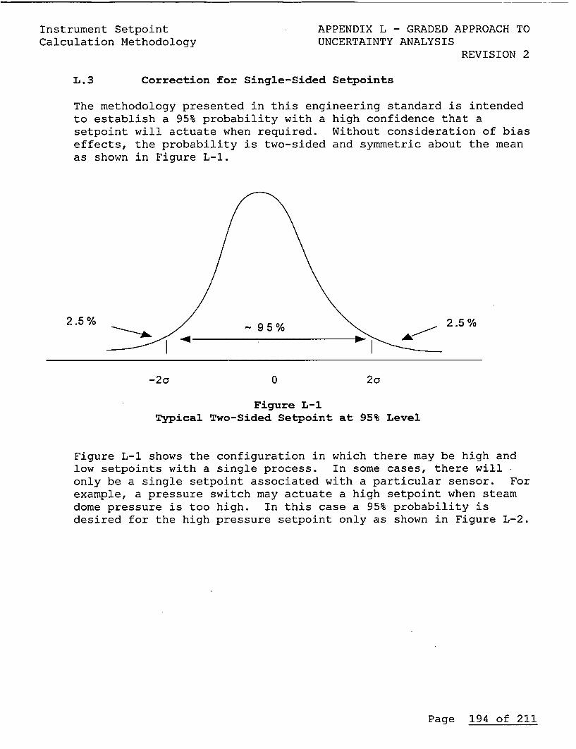
Instrument Setpoint APPENDIX L - GRADED APPROACH TOCalculation Methodology UNCERTAINTY ANALYSIS
REVISION 2
L.3 Correction for Single-Sided Setpoints
The methodology presented in this engineering standard is intendedto establish a 95% probability with a high confidence that asetpoint will actuate when required. Without consideration of biaseffects, the probability is two-sided and symmetric about the meanas shown in Figure L-1.
2.5 %- 95 % 2.5 %
_- . _
-2a 0 2a
Figure L-1Typical Two-Sided Setpoint at 95% Level
Figure L-1 shows the configuration in which there may be high andlow setpoints with a single process. In some cases, there willonly be a single setpoint associated with a particular sensor. Forexample, a pressure switch may actuate a high setpoint when steamdome pressure is too high. In this case a 95% probability isdesired for the high pressure setpoint only as shown in Figure L-2.
Page 194 of 211
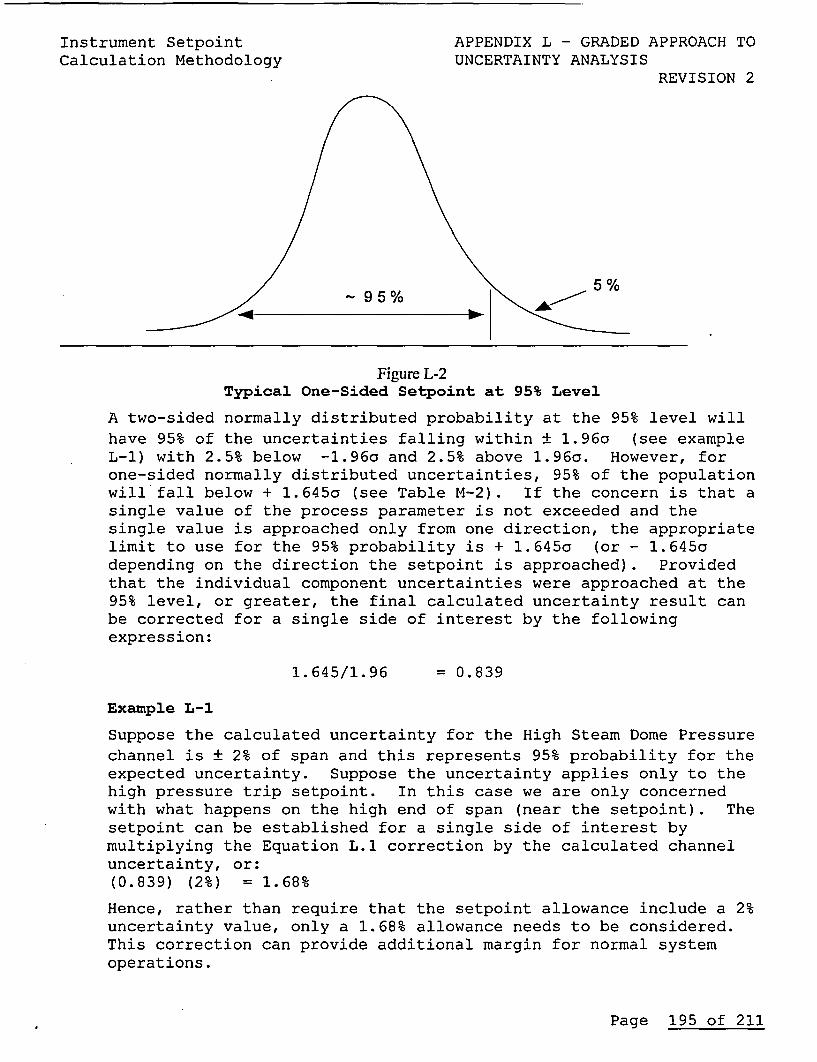
Instrument Setpoint APPENDIX L - GRADED APPROACH TOCalculation Methodology UNCERTAINTY ANALYSIS
REVISION 2
5 %
Figure L-2Typical One-Sided Setpoint at 95% Level
A two-sided normally distributed probability at the 95% level willhave 95% of the uncertainties falling within ± 1.96a (see exampleL-1) with 2.5% below -1.96c and 2.5% above 1.96a. However, forone-sided normally distributed uncertainties, 95% of the populationwill fall below + 1.645a (see Table M-2). If the concern is that asingle value of the process parameter is not exceeded and thesingle value is approached only from one direction, the appropriatelimit to use for the 95% probability is + 1.645a (or - 1.645adepending on the direction the setpoint is approached). Providedthat the individual component uncertainties were approached at the95% level, or greater, the final calculated uncertainty result canbe corrected for a single side of interest by the followingexpression:
1.645/1.96 = 0.839
Example L-1
Suppose the calculated uncertainty for the High Steam Dome Pressurechannel is ± 2% of span and this represents 95% probability for theexpected uncertainty. Suppose the uncertainty applies only to thehigh pressure trip setpoint. In this case we are only concernedwith what happens on the high end of span (near the setpoint). Thesetpoint can be established for a single side of interest bymultiplying the Equation L.1 correction by the calculated channeluncertainty, or:(0.839) (2%) = 1.68%
Hence, rather than require that the setpoint allowance include a 2%uncertainty value, only a 1.68% allowance needs to be considered.This correction can provide additional margin for normal systemoperations.
Page 195 of 211

Instrument SetpointCalculation Methodology
APPENDIX M - NOT USED
REVISION 2
APPENDIX M
NOT USED
Page 196 of 211
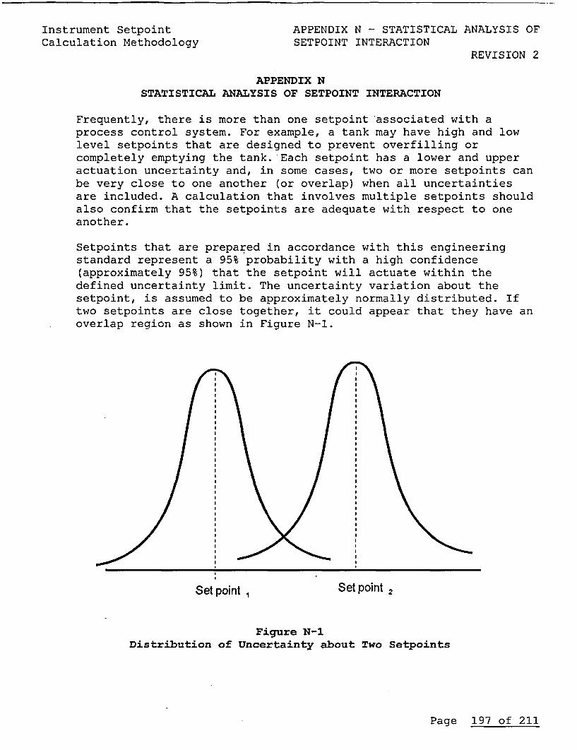
Instrument SetpointCalculation Methodology
APPENDIX N - STATISTICAL ANALYSIS OFSETPOINT INTERACTION
REVISION 2
APPENDIX NSTATISTICAL ANALYSIS OF SETPOINT INTERACTION
Frequently, there is more than one setpoint associated with aprocess control system. For example, a tank may have high and lowlevel setpoints that are designed to prevent overfilling orcompletely emptying the tank. Each setpoint has a lower and upperactuation uncertainty and, in some cases, two or more setpoints canbe very close to one another (or overlap) when all uncertaintiesare included. A calculation that involves multiple setpoints shouldalso confirm that the setpoints are adequate with respect to oneanother.
Setpoints that are prepared in accordance with this engineeringstandard represent a 95% probability with a high confidence(approximately 95%) that the setpoint will actuate within thedefined uncertainty limit. The uncertainty variation about thesetpoint, is assumed to be approximately normally distributed. Iftwo setpoints are close together, it could appear that they have anoverlap region as shown in Figure N-1.
Set point , Set point 2
Figure N-1Distribution of Uncertainty about Two Setpoints
Page 197 of 211
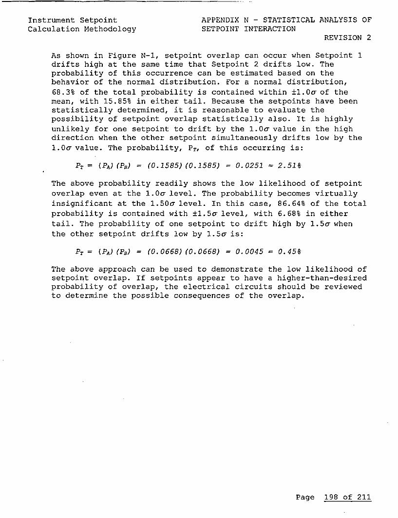
Instrument Setpoint APPENDIX N - STATISTICAL ANALYSIS OFCalculation Methodology SETPOINT INTERACTION
REVISION 2
As shown in Figure N-1, setpoint overlap can occur when Setpoint 1drifts high at the same time that Setpoint 2 drifts low. Theprobability of this occurrence can be estimated based on thebehavior of the normal distribution. For a normal distribution,68.3% of the total probability is contained within ±1.0o of themean, with 15.85% in either tail. Because the setpoints have beenstatistically determined, it is reasonable to evaluate thepossibility of setpoint overlap statistically also. It is highlyunlikely for one setpoint to drift by the 1.0o value in the highdirection when the other setpoint simultaneously drifts low by the1. Oa value. The probability, PT, of this occurring is:
PT = (PA) (PB) = (0.1585) (0.1585) = 0.0251 = 2.5196
The above probability readily shows the low likelihood of setpointoverlap even at the 1.0 level. The probability becomes virtuallyinsignificant at the 1.50a level. In this case, 86.64% of the totalprobability is contained with ±1.5a level, with 6.68% in eithertail. The probability of one setpoint to drift high by 1.5a whenthe other setpoint drifts low by 1.5a is:
PT = (PA) (PB) = (0. 0668) (0. 0668) = 0.0045 = 0.4596
The above approach can be used to demonstrate the low likelihood ofsetpoint overlap. If setpoints appear to have a higher-than-desiredprobability of overlap, the electrical circuits should be reviewedto determine the possible consequences of the overlap.
Page 198 of 211
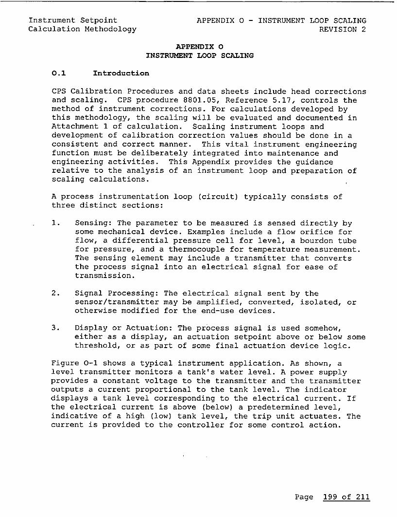
Instrument Setpoint APPENDIX 0 - INSTRUMENT LOOP SCALINGCalculation Methodology REVISION 2
APPENDIX 0INSTRUMENT LOOP SCALING
0.1 Introduction
CPS Calibration Procedures and data sheets include head correctionsand scaling. CPS procedure 8801.05, Reference 5.17, controls themethod of instrument corrections. For calculations developed bythis methodology, the scaling will be evaluated and documented inAttachment 1 of calculation. Scaling instrument loops anddevelopment of calibration correction values should be done in aconsistent and correct manner. This vital instrument engineeringfunction must be deliberately integrated into maintenance andengineering activities. This Appendix provides the guidancerelative to the analysis of an instrument loop and preparation ofscaling calculations.
A process instrumentation loop (circuit) typically consists ofthree distinct sections:
1. Sensing: The parameter to be measured is sensed directly bysome mechanical device. Examples include a flow orifice forflow, a differential pressure cell for level, a bourdon tubefor pressure, and a thermocouple for temperature measurement.The sensing element may include a transmitter that convertsthe process signal into an electrical signal for ease oftransmission.
2. Signal Processing: The electrical signal sent by thesensor/transmitter may be amplified, converted, isolated, orotherwise modified for the end-use devices.
3. Display or Actuation: The process signal is used somehow,either as a display, an actuation setpoint above or below somethreshold, or as part of some final actuation device logic.
Figure 0-1 shows a typical instrument application. As shown, alevel transmitter monitors a tank's water level. A power supplyprovides a constant voltage to the transmitter and the transmitteroutputs a current proportional to the tank level. The indicatordisplays a tank level corresponding to the electrical current. Ifthe electrical current is above (below) a predetermined level,indicative of a high (low) tank level, the trip unit actuates. Thecurrent is provided to the controller for some control action.
Page 199 of 211
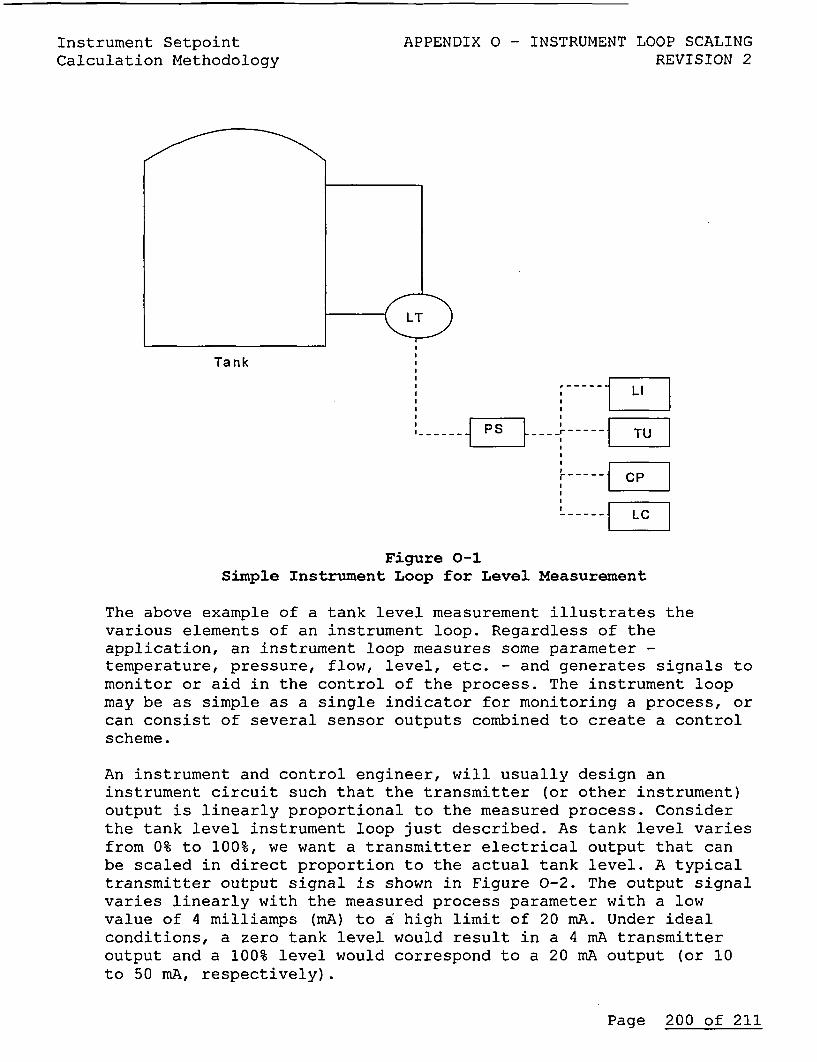
Instrument Setpoint APPENDIX 0 - INSTRUMENT LOOP SCALINGCalculation Methodology REVISION 2
Tank
ELEG
Figure 0-1Simple Instrument Loop for Level Measurement
The above example of a tank level measurement illustrates the
various elements of an instrument loop. Regardless of theapplication, an instrument loop measures some parameter -temperature, pressure, flow, level, etc. - and generates signals tomonitor or aid in the control of the process. The instrument loopmay be as simple as a single indicator for monitoring a process, orcan consist of several sensor outputs combined to create a controlscheme.
An instrument and control engineer, will usually design aninstrument circuit such that the transmitter (or other instrument)output is linearly proportional to the measured process. Considerthe tank level instrument loop just described. As tank level variesfrom 0% to 100%, we want a transmitter electrical output that canbe scaled in direct proportion to the actual tank level. A typicaltransmitter output signal is shown in Figure 0-2. The output signalvaries linearly with the measured process parameter with a lowvalue of 4 milliamps (mA) to a high limit of 20 mA. Under idealconditions, a zero tank level would result in a 4 mA transmitteroutput and a 100% level would correspond to a 20 mA output (or 10to 50 mA, respectively).
Page 200 of 211
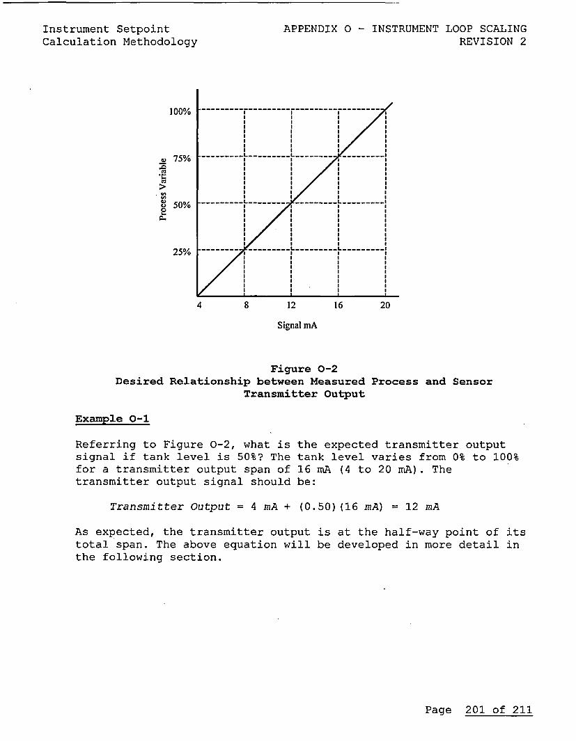
Instrument SetpointCalculation Methodology
100%
u 75%
.r
. rA
o 50%c-
25%
APPENDIX 0 - INSTRUMENT LOOP SCALINGREVISION 2
4 8 12 16 20
Signal mA
Figure 0-2Desired Relationship between Measured Process and Sensor
Transmitter Output
Example 0-1
Referring to Figure 0-2, what is the expected transmitter outputsignal if tank level is 50%? The tank level varies from 0% to 100%for a transmitter output span of 16 mA (4 to 20 mA). Thetransmitter output signal should be:
Transmitter Output = 4 mA + (0.50) (16 mA) = 12 mA
As expected, the transmitter output is at the half-way point of itstotal span. The above equation will be developed in more detail inthe following section.
Page 201 of 211
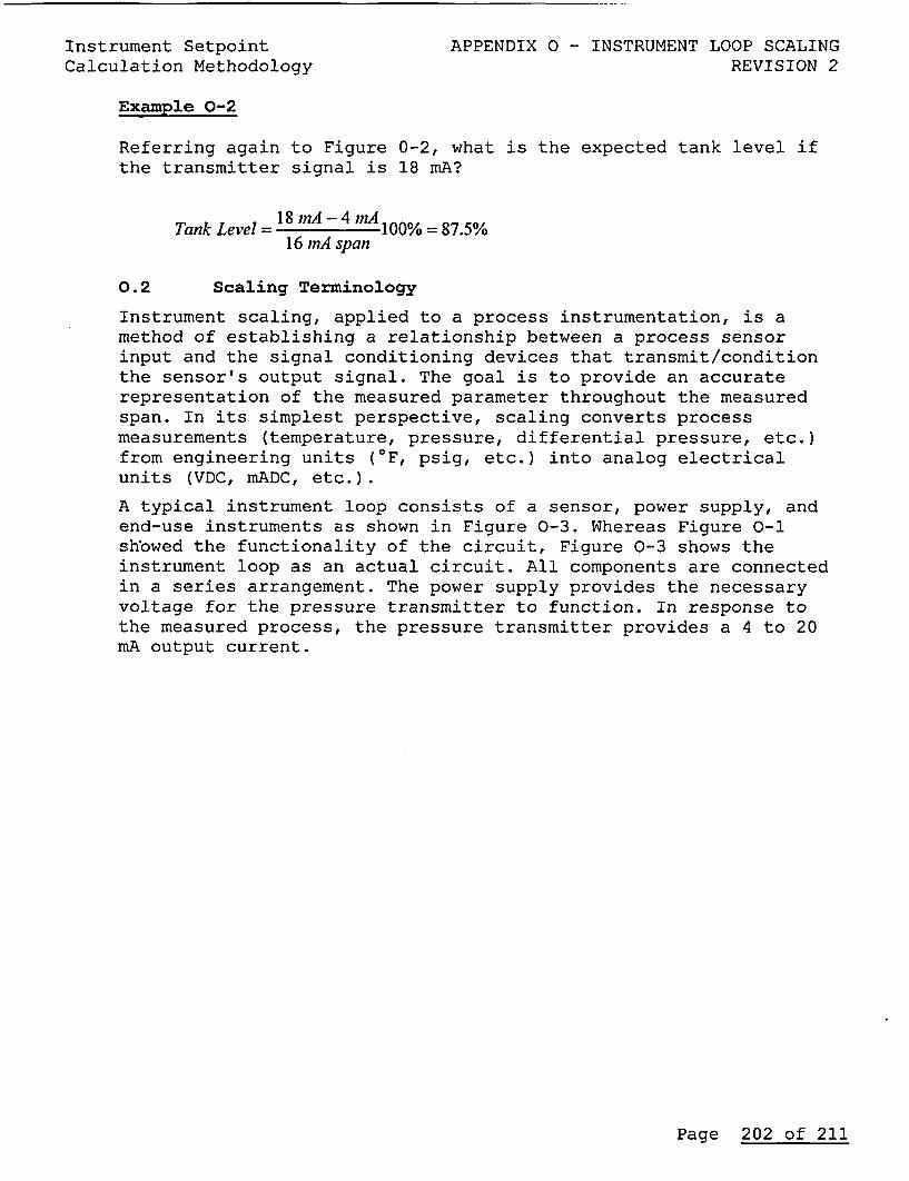
Instrument Setpoint APPENDIX 0 - INSTRUMENT LOOP SCALINGCalculation Methodology REVISION 2
Example 0-2
Referring again to Figure 0-2, what is the expected tank level ifthe transmitter signal is 18 mA?
18 mAd - 4 aTank Level =1mA-4nA10=87516 mA span
0.2 Scaling Terminology
Instrument scaling, applied to a process instrumentation, is amethod of establishing a relationship between a process sensorinput and the signal conditioning devices that transmit/conditionthe sensor's output signal. The goal is to provide an accuraterepresentation of the measured parameter throughout the measuredspan. In its simplest perspective, scaling converts processmeasurements (temperature, pressure, differential pressure, etc.)from engineering units (0F, psig, etc.) into analog electricalunits (VDC, mADC, etc.).
A typical instrument loop consists of a sensor, power supply, andend-use instruments as shown in Figure 0-3. Whereas Figure 0-1showed the functionality of the circuit, Figure 0-3 shows theinstrument loop as an actual circuit. All components are connectedin a series arrangement. The power supply provides the necessaryvoltage for the pressure transmitter to function. In response tothe measured process, the pressure transmitter provides a 4 to 20mA output current.
Page 202 of 211
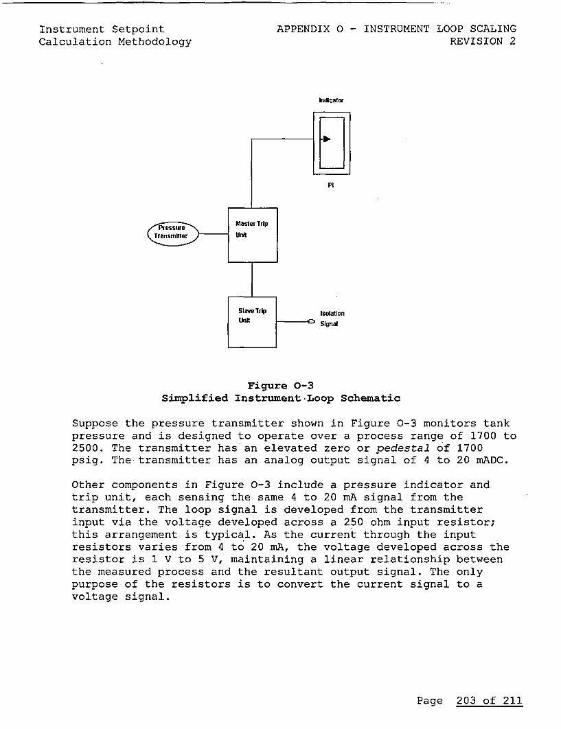
Instrument SetpointCalculation Methodology
APPENDIX 0 - INSTRUMENT LOOP SCALINGREVISION 2
Indicator
Pi
IsolationSignal
Figure 0-3Simplified Instrument-Loop Schematic
Suppose the pressure transmitter shown in Figure 0-3 monitors tankpressure and is designed to operate over a process range of 1700 to2500. The transmitter has an elevated zero or pedestal of 1700psig. The transmitter has an analog output signal of 4 to 20 mADC.
Other components in Figure 0-3 include a pressure indicator andtrip unit, each sensing the same 4 to 20 mA signal from thetransmitter. The loop signal is developed from the transmitterinput via the voltage developed across a 250 ohm input resistor;this arrangement is typical. As the current through the inputresistors varies from 4 to 20 mA, the voltage developed across theresistor is 1 V to 5 V, maintaining a linear relationship betweenthe measured process and the resultant output signal. The onlypurpose of the resistors is to convert the current signal to avoltage signal.
Page 203 of 211
Instrument Setpoint APPENDIX 0 - INSTRUMENT LOOP SCALINGCalculation Methodology REVISION 2
As configured in this example, the 1700 to 2500 psig process signalhas a span of 800 psig which corresponds to the 1 to 5 VDC (or 4VDC span) across the input resistor. The scale factor is defined asthe ratio of the analog electrical signal span to the process span,or 4 VDC/800 psig = 0.005 VDC/psig. Accounting for the 1700 psiginput pedestal and the 1 VDC output pedestal, the scaling equationthat relates the input to the output is given by:
Ep = [(0.005V/psig) (P - 1700 psig)] + 1V
where,
Ep =Voltage corresponding to the input pressure
P =Input pressure value between 1700 and 2500 psig
The above scaling equation provides an exact relationship betweenthe process variable and the voltage developed across an inputresistor for the stated configuration.
0.3 Module Equations
Module equations are commonly referred to as transfer functions.They define the relationship between a module's input and outputsignals and are just scaling equations that describe thisinput/output relationship. Transfer functions are typicallyclassified as either static or dynamic.
Static transfer functions are time-independent and can be eitherlinear or nonlinear. Modules that typically have static transferfunctions include:
* Input resistors (I/V modules)* Isolators* Summators
Page 204 of 211
Instrument Setpoint APPENDIX 0 - INSTRUMENT LOOP SCALINGCalculation Methodology REVISION 2
The module equation of a static device will sometimes include again adjustment also. For example, a simple summator may have thefollowing module equation:
E.,y= G(k1El + k2E2 + kBEB) + 1 V
where,
k1 , k2 Input signal gains
kB = Bias input gain
El, E2 = Input voltages
EB Bias voltage
G = Output gain
E0ut = Output voltage
0.4 Scaling calculation
After the process algorithm, module equations, and required rangeshave been determined, the scaling calculation can be completed. Thescaling factor is used with the scaling equation to derive thevoltage equation form the process equation. An overall systemequation can be developed, by combining module equations, asapplicable. For example, assume the use of two modules in aninstrument loop.
The first module has two inputs, Eland E2, that are summed togetherwith a module gain of G1. The simplified equation for this module.isgiven by:
EA = GI (El + E2 )
Now, assume that the output, EA, is summed with another input, E3 ,which has a module gain of G2. The resulting module equation is:
Eout = G2 (E 3 + EA)
or, substituting in for EA,
E.., = G2 [E3 + GI(El + E2)]
Page 205 of 211
Instrument Setpoint APPENDIX 0 - INSTRUMENT LOOP SCALINGCalculation Methodology REVISION 2
The expression for each voltage above can be complex also. But, theresult is an overall scaling equation that defines the systemoperation. Once a scaling equation has been developed and thescaling calculation performed, the equation should be checked byinputting typical process values and determining if reasonableanalog values are calculated. Each module should be testedseparately to ensure its accuracy before combining it with othermodules. As part of the test process, include minimum and maximumprocess values to ensure that the limits work as expected.
Page 206 of 211
Instrument Setpoint APPENDIX P - RADIATION MONITORINGCalculation Methodology SYSTEMS
REVISION 2
APPENDIX PRADIATION MONITORING SYSTEMS
Radiation monitoring systems have unique features that complicate anuncertainty analysis. The system design, detector calibration, anddisplay method all can reduce the system accuracy. Wheneverevaluating a radiation monitoring system, review References 5.9 and5.33, for additional information and:
Radiation monitoring system operation and maintenance manual
Radiation monitoring system calibration procedures
The following should be considered as part of any uncertaintyanalysis:
Detector Measurement Uncertainty
A radiation monitoring system detector's response varies with thefollowing parameters:
* Energy level of the incident particles.
* Count rate of the detected particles.* Type of particle being counted (depending on application, the
particles may be gamma photons, neutrons, or beta particles).
Detector Count Rate Measurement Uncertainty
The detector's measurement uncertainty can be affected by thefollowing:
* On the low end of scale, the uncertainty in count rate responseis affected by signal to noise ratio effects.
* On the high end of scale, the uncertainty in count rate isaffected by pulse pile-up in which discrete pulses are missed.
* Through the detection range, the alignment of the source to thedetector geometry can impact the measurement uncertainty. Forexample, the containment high range radiation monitors need anunobstructed view of the containment dome. Blockages such asconcrete walls can degrade the measurement capability of thedetector.
Detector Energy Response Uncertainty
The detector energy response uncertainty can be affected by thefollowing:
Page 207 of 211
Instrument Setpoint APPENDIX P - RADIATION MONITORINGCalculation Methodology SYSTEMS
REVISION 2* On the low end, the discriminator setting and the energy
sensitivity of the detector.
* On the high end, the point at which a rise in incident particleenergy does not result in a change in pulse height output.
* Throughout the detection range, by a degrading failure of thesystem.
For most permanently installed radiation detectors, the detector isdesigned to respond to incident particles over a certain range ofenergies. The output of count rate is then correlated to a mR/hr
or pC/cc indication by the application of a conversion factor,without regard to differing incident particle energies.
When the plant is shutdown, the detector indicated count rate isgenerally derived from lower energy particles. When the plant isoperating, the particle energy tends to be higher. In this case, atypical detector will display a higher count rate, even if thenumber of incident particles per unit time remains the same. As theincident particle energy level changes, the probability of detectionchanges, for a given count rate. During initial calibration, thisdifference is accounted for by exposing the detector sample streamsof different radioisotopes and measuring the detector's response.After in-plant installation, the calibration is checked, by exposingthe detector to fixed external sources of different radioisotopes.
The detector coefficient represents the sensitivity of the detector,which is typically specified in Amp/(R/hr). The sensitivity isprovided by the vendor for each detector and can be different if thedetectors are ever replaced.
Post Accident Radiation Measurement and Indication accuracy forcontainment area monitoring, is specified in Regulatory Guide 1.97,Table 2, Footnote 7. "Detectors should respond to gamma radiationphotons, within any energy range from 60 keV to 3 MeV with an energyresponse accuracy of "20% at any specific photon energy from 0.1 MeVto 3 MeV". Overall system accuracy should be within a factor of 2over the entire range." Revision 3 of R.G. 1.97 revised the abovefootnote to omit the "20% accuracy requirement for the detector.Now the containment area radiation monitors "should respond to gammaradiation photons within any energy range from 60 keV to 3 MeV witha dose rate response accuracy within a factor of 2 over the entirerange". Considering the prior revision, it is clear the intent ofthe "factor of 2" current requirement applies to the "overall systemaccuracy" and not the detector accuracy alone. This interpretationis consistent with the requirements placed on other radiationmonitoring devices in the same table.
Page 208 of 211
Instrument Setpoint APPENDIX P - RADIATION MONITORINGCalculation Methodology SYSTEMS
REVISION 2The uncertainty terms identified in radiation monitoringtechnologies are either percent of reading or in Equivalent LinearFull Scale (ELFS), which is the same as percent of span provided thespan and full scale are equivalent. The method for convertingpercent of reading uncertainties to percent ELFS using the "errorfactor" concept is based on the model from an example radiation tripcalculation in Reference 5.3, ISA S 67.04 Part II.Conversion of this error to an ELFS error permits combining thepercent of reading error with other string errors.
Consider the following example; A containment area monitor indicatesR/Hr over an eight (8) decade range, uncertainty is calculated forthe detector at 12.2%.
This detector accuracy error can be expressed as error factors of:(1.0 + 0.122)/1.0 = 1.122 and (1.0 - 0.122)/1.0 = 0.878. ELFS iscalculated for both factors as:
ERROR FACTOR = loDX, where D = 8, the number ofdecades on the meter and X =
ELFS as a decimal value.
X(+) = (log(l.122)/8) * 100%= +0.62% ELFSX(-) = (log(0.878)/8) * 100%= - 0.71% ELFS
The error will be assumed to be symmetrical and set at thelarger of two values, thus EDET(ref) = "0.71 % ELFS.
Whenever evaluating the uncertainty of a radiation monitoringsystem, the periodic calibration methods are particularly importantto consider. EPRI TR-102644, Reference 5.33, provides additionalguidance. Also, the applicable system engineer should be contactedfor additional expertise.
Page 209 of 211
Instrument Setpoint APPENDIX Q - ROSEMOUNT LETTERSCalculation Methodology REVISION 2
APPENDIX Q
Rosemount Nuclear Instruments Rosemount Nuclear Instruments. Inc.12001 Technology DriveEden Prairie, MN 55344 USATel 1 (612) 828-8252Fax 1 (612) 828-8280
4 April 2000.
Ref: Grand Gulf Nuclear Station message on INPO plant reports, subject Rosemount Instrument SetpointMethodology, dated March 9, 2000
Dear Customer:
This letter is intended to eliminate any confusion that may have arisen as a result of the reference message from GrandGulf. The message was concerned with statistical variation associated with published performance variables and howthe variation relates to the published specifications in Rosemount Nuclear Instruments, Inc.(RNII) pressure transmittermodels 1152, 1153 Series B, 1153 Series D, 1154 and 1154 Series H. According to our understanding, theperformance variables of primary concern are those discussed in GE Instrument Setpoint Methodology documentNEDC 31336, namely
1. Reference Accuracy2. Ambient Temperature Effect3. Overpressure Effect4. Static Pressure Effects5. Power Supply Effect
It is RNII's understanding that GE and the NRC have accepted the methodology of using transmitter testing to insurespecifications are met as a basis for confirming specifications are ±3o, The conclusions we draw regardingspecifications being ±3o are based on manufacturing testing and screening, final assembly acceptance testing, periodic(e.g., every 3 months) audit testing of transmitter samples and limited statistical analysis. Please note that allperformance specifications are based on zero-based ranges under reference conditions. Finally, we wish to make clearthat no inferences are made with respect to confidence levels associated with any specification.
1. Reference Accuracy.
All (100%) RNII transmitters, including models 1152, 1153 Series B, 1153 Series D, 1154 and 1154 Series H, aretested to verify accuracy to ±0.25% of span at 0%, 20%, 40%, 60%, 80% and 100% of span. Therefore, thereference accuracy published in our specifications is considered ±3a.
2. Ambient Temperature Effect
All (100%) amplifier boards are tested for compliance with their temperature effect specifications prior to finalassembly. All sensor modules, with the exception of model 1154, are temperature compensated to assurecompliance with their temperature effect specifications. All (100%) model 1154, model 1154 Series H and model1153 gage and absolute pressure transmitters are tested following final assembly to verify compliance withspecification. Additionally, a review of audit test data performed on final assemblies of model 1152 and model I153 transmitters not tested following final assembly indicate
FISHER-ROSEMOUNT
conformance to specification. Therefore, the ambient temperature effect published in our specifications isconsidered ±3a
Page 210 of 211
Instrument Setpoint.Calculation Methodology3. Overpressure Effect
APPENDIX Q - ROSEMOUNT LETTERSREVISION 2
Testing of this variable is done at the module stage. All (100%) range 3 through 8 sensor modules are tested forcompliance to specifications. We do not test range 9 or 10 modules for overpressure for safety reasons. However,design similarity permits us to conclude that statements made for ranges 3 through 8 would also apply to ranges 9and 10. Therefore, the overpressure effect published in our specifications is considered ±3a.
4. Static Pressure Effects
All (100%) differential pressure sensor modules are tested for compliance with static pressure zero errors.Additionally, Models 1153 and 1154 Ranges 3, 6,7 and 8 are 100% tested after final assembly for added assuranceof specification compliance. Audit testing performed on ranges 4 and 5 have shown compliance to the specification.Therefore, static pressure effects published in our specifications are considered ±3G.
5. Power Supply Effect
Testing for conformance to this specification is performed on all transmitters undergoing sample (audit) testing.This variable has historically exhibited extremely small performance errors and small standard deviation(essentially a mean error of zero with a standard deviation typically less than 10% of the specification). Alltransmitters tested were found in compliance with the specification. Therefore, power supply effect published in ourspecifications is considered ±3a.
Should you have any further questions, please contact Jerry Edwards at (612) 828-3951.
Sincerely,
Jerry L. Edwards Manager, Sales, Marketing and Contracts Rosemount Nuclear Instruments, Inc.
FISIIER-ROSENIOUNT
Page 211 of 211
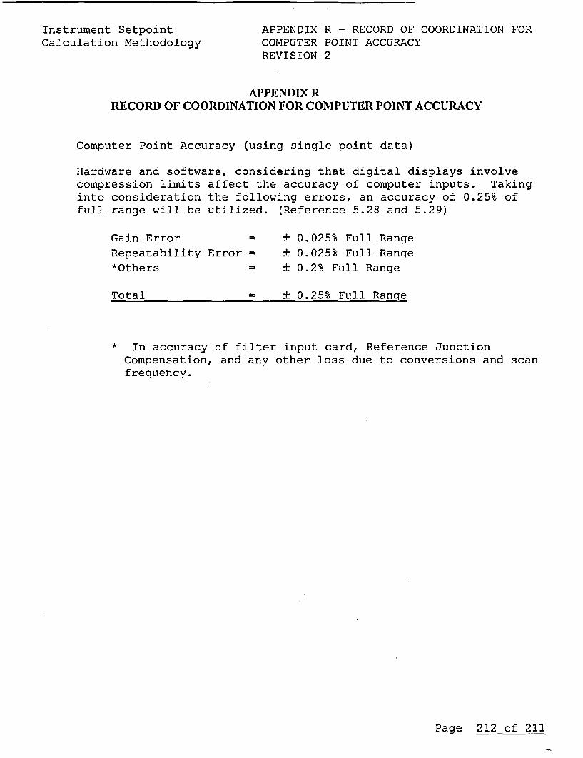
Instrument SetpointCalculation Methodology
APPENDIX R - RECORD OF COORDINATION FORCOMPUTER POINT ACCURACYREVISION 2
APPENDIX RRECORD OF COORDINATION FOR COMPUTER POINT ACCURACY
Computer Point Accuracy (using single point data)
Hardware and software, considering that digital displays involvecompression limits affect the accuracy of computer inputs. Takinginto consideration the following errors, an accuracy of 0.25% offull range will be utilized. (Reference 5.28 and 5.29)
Gain Error
Repeatability Error =*Others
Total
± 0.025% Full Range± 0.025% Full Range± 0.2% Full Range
± 0.25% Full Range
* In accuracy of filter input card, Reference JunctionCompensation, and any other loss due to conversions and scanfrequency.
Page 212 of 211