Attention in Games: An Experimental Study∗

Ala Avoyan† and Andrew Schotter ‡

September 2016

Abstract

One common assumption in game theory is that players concentrate on one

game at a time. However, in everyday life, we play many games and make many

decisions at the same time, and thus have to decide how best to divide our limited

attention across these settings. The question posed in this paper is how do people

go about solving this attention-allocation problem, and how does this decision affect

the way players behave in any given game when taken in isolation. We ask: What

characteristics of the games people face attract their attention, and does the level

of strategic sophistication exhibited by a player in a game depend on the other

games he or she is engaged in? We find there is a great deal of between-game inter

dependence which implies that if one wants to fully understand why a player in a

game acts in a particular way, one would have to take a broader general-equilibrium

view of the problem and include these inter-game effects.

JEL Classification: C72, C91, C92, D83; Keywords: Inattention, Games,

Attention Allocation, Bounded Rationality.

∗We would like to thank Andrew Caplin, Ariel Rubinstein, Guillaume Frechette, Xavier Gabaix, LarbiAlaoui, Miguel A. Ballester, Mark Dean, David Laibson, Graham Loomes, Antonio Penta, Giovanni Ponti,Matthew Rabin, David Rand and Jakub Steiner for their helpful comments. This paper also benefitedfrom comments received by conference participants at the “Typologies of Boundedly Rational Agents:Experimental Approach”, held in Jerusalem in June 2015, 2015 ESA North American meetings, BarcelonaGSE Summer Forum and Stanford Institute for Theoretical Economics (SITE) Conference. We gratefullyacknowledge financial support from the Center for Experimental Social Science at New York University(CESS), and software assistance from Anwar Ruff.†Department of Economics, New York University. E-mail: a.avoyan@nyu.edu‡Department of Economics, New York University. E-mail: andrew.schotter@nyu.edu

1

1 Introduction

When studying or teaching game theory, one common assumption is that people play

or concentrate on one game at a time. We typically analyze player’s behavior in the

Prisoners’ Dilemma, the Battle of the Sexes, or more sophisticated dynamic games in

isolation. In everyday life, however, we play many games and make many decisions at the

same time, and have to decide how to split our limited attention across all these settings.

The main question we pose in this paper is, how do people go about solving this

attention-allocation problem? In particular, what characteristics of the games people face

attract their attention and lead them to focus more on those problems rather than others;

do people concentrate on the problems that have the greatest downside or the ones with

the greatest upside payoffs; and do they pay more attention to games which are more

complicated from a game-theoretical point of view, or maybe the payoff characteristics of

the games trump these strategic considerations?

We view behavior in any given game as being determined by two factors. The first,

as mentioned above, is how much attention a player decides to give to a game, given

the other games he simultaneously faces. The second is how a player behaves given this

self-imposed attentional constraint.

To discuss the first factor we use a modified version of Koszegi and Szeidl (2013)

(hereafter, KS) as a vehicle to structure our thinking. Other models could be used to

equal advantage including an adaptation of the Alaoui and Penta (2015) model,1 used to

endogenously determine the level of strategic sophistication people use when playing a

given game in isolation, or the models of Bordalo et al. (2012) which concerns the saliency

of lottery attributes (prizes and probabilities) or Bordalo et al. (2016) where the salience

of goods defined by their price and quality compete for the attention of consumers in a

market (see also Cunningham (2011) and Bushong et al. (2015)).2 In all of these models

the objects vying for attention all have multiple attributes. We extend (to our knowledge,

for the first time) the use of such models to study attention in games (objects which also

have multiple attributes).

We have adopted the Koszegi and Szeidl (2013) model because it presents an analysis

1 We would like to thank Larbi Alaoui and Antonio Penta for making us aware of exactly how onecould adapt their model, created to describe the endogenous determination of level-k within a givengame to a multi-game setting sutch as ours. Even more appreciated is an analysis they did detail-ing how their model could be applied to our problem. For details see Alaoui and Penta (2016), athttp://www.econ.wisc.edu/apenta/EDRandRT.pdf.

2 Gabaix (2011) redoes consumer theory using his sparse max analysis where the consumer needs todecide how much attention to pay to the prices of goods he faces. Such attention allocation in his modeldepends on how variable the price of a good is and its elasticity of demand.

2

that is closest to our intuition about the problem of attention allocation. However, the

purpose of our paper is not to test the KS model (see Andersson et al. (2016) for a direct

test). While it does help us structure our discussion and provides theoretical support for

many of our conjectures, our paper deals with a number of issues that are outside of the

KS framework. Nevertheless, as stated above, KS does provide a very nice structure that

organizes our thinking.

In terms of our second factor, there is ample evidence that the level of sophistication

one employs in a game depends on how much time or attention is devoted to it. For

example, Agranov et al. (2015) allow players two minutes to think about engaging in a

beauty-contest game. At each second the players can change their strategy, but at the

end of the two minutes one of the times will be chosen at random, and the choice at that

time will be payoff relevant. The design makes it incentive compatible at each point in

time for the subject to enter his or her best guess as to what is the most beneficial choice

to make.

What these authors show is that, as time goes on, those players who are not acting

randomly (level-zeros, perhaps) change their strategies in the direction of the equilibrium.

Hence, Agranov et al. (2015) results suggest that the level-k chosen is a function of

contemplation time or that, as Rubinstein (2016) proposes, as more time is allocated to

the game people switch from an intuitive to a more contemplative strategy.

In a similar vein, Lindner and Sutter (2013), using the 11-20 Game of Arad and

Rubinstein (2012), find that, if you impose time limits on subjects who play this game,

the choice made by subjects changes in the direction of the equilibrium. As Lindner and

Sutter (2013) suggest, this might be the result of the fact that imposing time constraints

forces subjects to act intuitively (Rubinstein (2016)) and such fast reasoning leads them

to choose lower numbers.3 Rand et al. (2012) find that as people are allowed more time to

think about their contribution in a public goods game, their contributions falls.4 Finally,

Rubinstein (2016) reverses the causality and looks at the decision times used by subjects

to make their decisions in situations and infers the type of decision they are making

(intuitive or contemplative) from their recorded decision time. What is important for our

purposes is that as people pay more attention to a game their behavior changes.

One corollary of our analysis is the fact that we describe how the behavior of an agent

3 See also Schotter and Trevino (2014) for a discussion on use of response times as a predictor ofbehavior.

4 See Recalde et al. (2014) for a discussion of decision times and behavior in public goods games andthe influence of mistakes. See Kessler et al. (2015) for behavior in Prisoners’ Dilemma and Dictator Gamemade with more or less time and various incentives.

3

engaged in one specific game is affected by the type of other games he is inter-acting in.

We provide results that indicate that the level of sophistication one employs in a game

is determined endogenously and depends on the constellation of other games the person

is engaged in and the resulting attention he allocates to the game under consideration.

In other words, if one aims to explain the behavior of a person playing a game in the

real world, one must consider the other games that person is simultaneously engaged

in. While others like Choi (2012) or Alaoui and Penta (2015) have provided models of

the endogenous determination of sophistication within one game, we expand this focus

and look to include more general-equilibrium like inter-game factors.5 This result follows

naturally from our study on attention allocation in games.

To answer the questions we pose, we conduct an experiment where we present subjects

with a sequence of pairs of matrix games shown to them on a screen for a limited amount

of time (10 seconds), and ask them which of the two games displayed would they like

to allocate more time to thinking about before they play them at the end of the experi-

ment. In other words, the main task in the experiment is not having subjects play games

but presenting them with pairs of games and asking them to allocate a fixed budget of

contemplation time between them. These time allocations determine how much time the

subjects will have to play these games at the end of the experiment.

In addition to these questions, we also investigate whether subjects’ attention allo-

cation behavior is consistent. For example, are these allocation times transitive in the

sense that if a subject reveals that he would want to allocate more time to game Gi when

paired with game Gj and game Gj when paired with game Gk, then would he also allocate

more time to game Gi when paired with game Gk? Other consistency conditions are also

examined.

Finally, we also ask what it means for a player to decide that he would like to pay

more attention to one game rather than another. Does it mean that he likes or would

prefer to play that game more than the other, or does it mean the opposite, i.e., he dreads

playing that game and for that reason feels he needs to think more about it? To answer

these types of questions we run a separate treatment where subjects are presented the

same game pairs as in our original experiment but, instead of allocating contemplation

time across these games, they are asked which one they would prefer to play at the end

of the experiment. All of this information, both for attention time and game preference

is elicited in an incentive compatible way with payoff-relevant choices.

5 Bear and Rand (2016) theoretically analyze agents’ strategies when they are sequentially playingmore than one type of game over time. For the effects of simultaneous play, cognitive load and spilloverson strategies see Bednar et al. (2012) and Savikhin and Sheremeta (2013).

4

What we find is interesting. First, we present evidence that clearly demonstrates that

how a subject behaves when playing a given game varies greatly depending on the other

game he or she is engaged in. This directly supports our conjecture that a key element in

determining how a player behaves in a given game is the set of other games he or she is

simultaneously engaged in, and that the proper study of strategic behavior must include

these interconnected elements. In this sense, conventional game theory presents a type of

partial equilibrium analysis.

With respect to the allocation of time across games, we find that subjects respond

to both the strategic elements of the games presented to them and their payoffs. For

example, subjects on average allocate more time to Prisoners’ Dilemma (PD) games than

any other type or class of game shown to them, followed by Constant Sum games (CS)

and then Battle of the Sexes games (BoS). They pay the least amount of attention to

Pure Coordination games (PC), although the difference between the time allocated to

Pure Coordination and Battle of the Sexes games is only marginally significant.

This does not, by any means, suggest that strategic factors alone determine allocation

times, however. Payoffs are also relevant. For instance, subjects allocate less time to

matrix games where some payoffs are zero in comparison to otherwise-identical games

where all payoffs are positive. They also allocate more time to games as their payoffs

increase holding the payoffs in the comparison game constant. In addition, the time

allocated to different games in the same game class, such as different PD games, when

compared to an identical other game (such as a BoS game), varies according to the payoff

of the PD games. This may be interesting in the sense that game theorists might think

that once a subject identifies a game as being in a particular class, like the class of PD

games, then the amount of time allocated to that game might be invariant to payoff

changes in those games, since despite their different payoffs, all games in the same game

class are strategically equivalent, i.e., a PD game is a PD game is a PD game. This might

be the view of those who view allocation time to be a function of game complexity and,

since all PD games are of identical strategic complexity, they all would require the same

attention allocated to them no matter what their payoffs are. Our data demonstrates

that this is not the case. Different members of a game class when compared to identical

other games elicit different allocation times.

In terms of consistency, we find that while our subjects acted in a generally consistent

manner, on various consistency measures they also exhibited considerable inconsistency.

In terms of transitivity, however, our subjects appeared to be remarkably consistent in

that over 79% of subjects exhibited either 0 or 1 intransitive allocation times when three

5

pairs of connected binary choices were presented to them. Other consistency metrics,

however, provide evidence of substantial inconsistency.

Finally, it appears that the amount of time allocated to thinking about a game is

positively related to a subject’s preference for that game. One interesting exception is

Pure Coordination games since subjects allocate relatively little time to them but state

that they prefer playing them. This is because subjects seem to recognize the simplicity

of these games compared, let’s say, to constant sum games, and hence decide to spend

their time elsewhere.

We will proceed as follows. In Section 2 we describe our experimental design. In

Section 3 we present our adapted version of the KS model as applied to our time-allocation

problem. In section 4 we outline a set of intuitive conjectures, some of which (concerning

attention allocation) follow from the KS model, about the type of behavior we expect

to see in our experiment. In Section 5 we reformulate these conjectures as statistical

hypotheses and present our results. Section 6 concludes the paper.

2 Experimental Design6

The experiment was conducted at the Center for Experimental Social Science (CESS)

laboratory at New York University (NYU) using the software z-Tree (Fischbacher (2007)).

All subjects were NYU undergraduates recruited from the general population of NYU

students. The experiment lasted about one hour and thirty minutes and, on average,

subjects received $21 for their participation. The experiment consisted of two different

treatments run with different subjects. In one, subjects were asked to allocate time

between two or sometimes three games. In the other, subjects were asked to choose which

game they would prefer to play. We will call these the Time-Allocation Treatment and

the Preference Treatment. The experiment run for each treatment consisted of a set of

tasks which we will describe below.

2.1 Time-Allocation Treatment

2.1.1 Task 1

Comparison of Game-Pairs In the first task of the Time-Allocation Treatment there

were 45 rounds. In each of the first 40 rounds subjects were shown a pair of matrix games

(almost always 2×2 games) on their computer screen (we will discuss the final five round

in the next subsection). Each matrix game presented a situation where two players had

to choose actions which jointly determined their payoffs. In the beginning of any round a

6 Instructions used in our experiment can be found in Appendix D and E.

6

pair of matrix games would appear on their screen for 10 seconds. Subjects were not asked

to play these games but rather they were asked to decide how much time they would like

to allocate to thinking about them if they were offered a chance to play these games at the

end of the experiment. To make this allocation the subjects had to decide what fraction

of X seconds they would allocate to Game 1 (the remaining fraction would be allocated

to Game 2). The value of X was not revealed to them at this stage, however. Rather

they were told that X would not be a large amount of time, hence, what they needed

to decide upon in Task 1 was the relative amounts of time they would like to spend

contemplating these two games if they were to play them at the end of the experiment.

We did not tell subjects how large X was since we wanted them to anticipate being

somewhat time constrained when they had to play these games that is, we wanted the

shadow price of contemplation time to be positive in their mind. We feared that if they

perceived X to be so large that they could fully analyze each game before deciding, they

might feel unconstrained and allocate 50% to each game. Avoiding this type of strategy

was important since what we are interested in is the relative amounts of attention they

would like to allocate to each game. We wanted to learn which game they thought they

needed to attend to more. Our procedure, we felt, was suited to this purpose well.

To indicate how much time they wanted to allocate to each game the subjects had

to write a number between 0 and 100 to indicate the fraction or percentage of time they

wanted to allocate to thinking about the game designated as Game 1 on their screen. The

remaining time was allocated to Game 2. To do this, we allowed subjects to view each

pair of games for 10 seconds and then gave them 10 seconds to enter their percentage. We

limited them to 10 seconds because we did not want to give them enough time to actually

try to solve the games but rather to indicate which game appeared more worthy of their

attention later. We expected them to view the games, evaluate their features, and decide

how much the relative amounts of attention they would like to allocate to these games if

they were to play them later on.

On the screen displaying the two games was a counter in the right hand corner indi-

cating how much time they had left before the screen would go blank and they would be

asked to enter their attention percentage in a subsequent screen which also had a counter

in the right-hand corner.

<Figure 6> <Figure 7>

One of the games used for comparison was different from the others in that in involved

chance and hence is called the Chance Game. When a subject had to choose between two

7

games, one being a chance game, the subject’s screen appeared as in Figure 7. What this

says is that subjects will need to allocate time between Game 1 and Game 2 – the Chance

Game. Game 2 says that with probability 12

subjects will play the top game on the screen

and with probability 12

they will play the bottom game. However, in the Chance Game

subjects must make a choice, A or B, before knowing exactly which of those two games

they will be playing, that is determined by chance after their A/B choice is made. Note

that strategically the chance game is identical to a pure coordination game (see game

PC500 in Table 1).

2.1.2 The Last Five Rounds: Comparisons of Triplets

When 40 rounds were over, subjects were given 5 triplets of games to compare. In each

of these last 5 rounds they were presented with three matrix games on their screens and

given 20 seconds to inspect them. As in the first 40 round task, subjects were not asked

to play these games but rather to enter how much time out of 100% of total time available

they would allocate to thinking about each of the games before making a decision. To

do this, when the screen went blank after the description of the games, subjects had 20

seconds to enter the percentage of total time they wanted to allocate to thinking about

Game 1 and Game 2 (the remaining seconds were allocated to thinking about Game 3).

After the choice for the round was made subjects had some time to rest before the next

pair of problems was presented for which they repeated the same process.

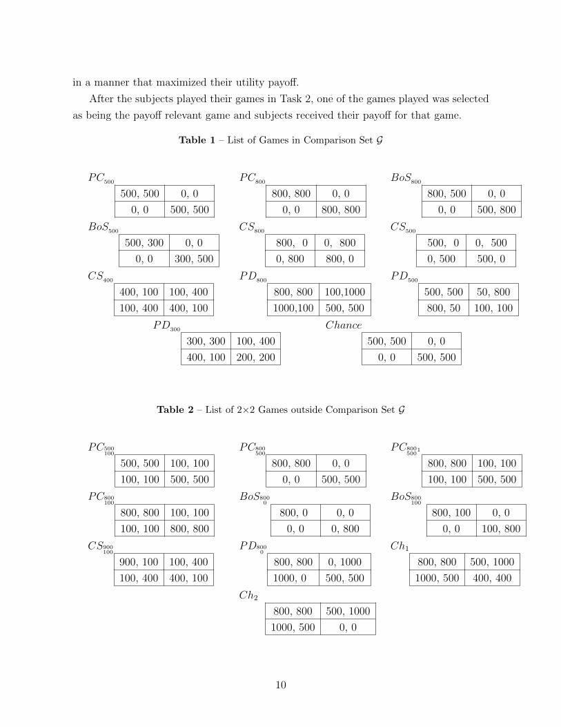
All of the games that were used to make comparisons are in Tables 1, 2, 3 and 4. In

total, there were 25 games used, ranging from Prisoners’ Dilemma, Pure Coordination,

Constant Sum, Games of Chicken, and variants on these games. Of the 25 games 21 were

2×2 games with 2 games being 2×3 and 2 games being 3×3. Of the 25 games used, there

were a set of 11 games where each game in the set was compared to every other. This

set, called the Comparison Set G below, will be a central focus for us since it will allow

us to compare how any two games attracted consideration time when compared to the

same set of games. In other words, games in the Comparison Set G allow us to hold the

games compared constant when evaluating whether one game attracted more attention

than another.

2.1.3 Task 2: Playing Games and Payoffs

In terms of payoffs, what the subjects were told is that at the end of the 45 rounds two

of the 45 pairs of games they saw in Task 1 would be presented to them again at which

time they would have to play these games by choosing one of the strategies available to

them (they always played as Row players). For each pair of games they were allowed an

8

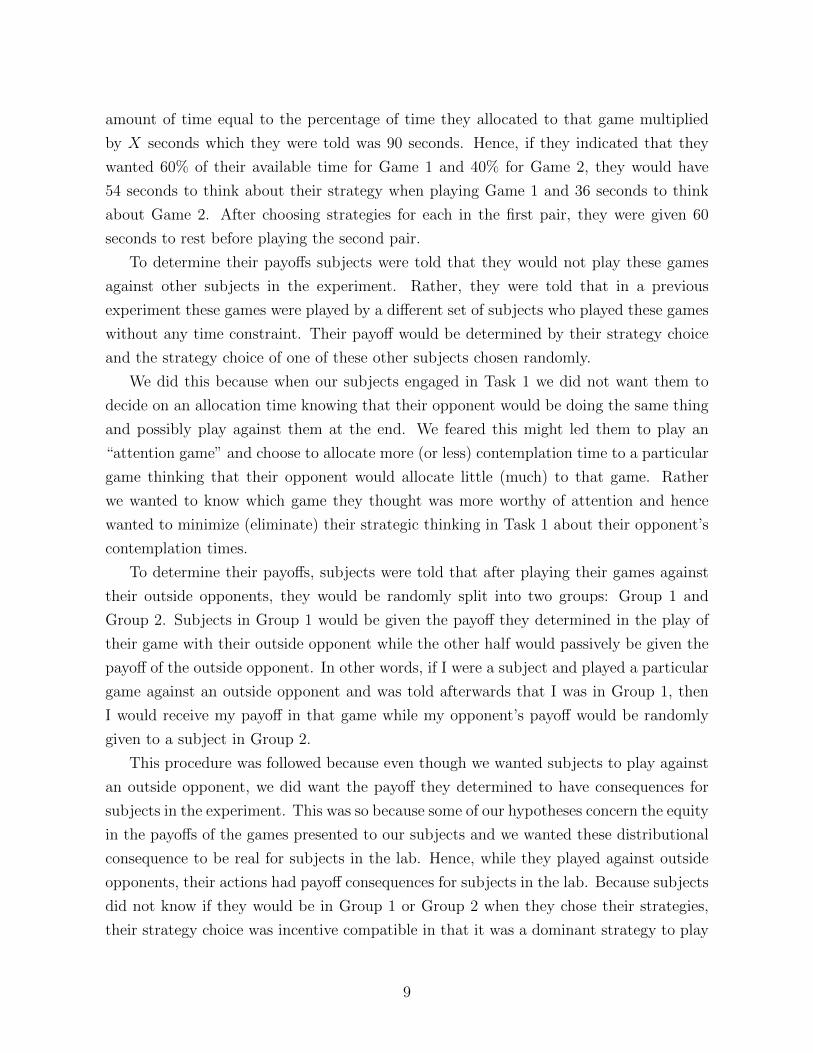
amount of time equal to the percentage of time they allocated to that game multiplied

by X seconds which they were told was 90 seconds. Hence, if they indicated that they

wanted 60% of their available time for Game 1 and 40% for Game 2, they would have

54 seconds to think about their strategy when playing Game 1 and 36 seconds to think

about Game 2. After choosing strategies for each in the first pair, they were given 60

seconds to rest before playing the second pair.

To determine their payoffs subjects were told that they would not play these games

against other subjects in the experiment. Rather, they were told that in a previous

experiment these games were played by a different set of subjects who played these games

without any time constraint. Their payoff would be determined by their strategy choice

and the strategy choice of one of these other subjects chosen randomly.

We did this because when our subjects engaged in Task 1 we did not want them to

decide on an allocation time knowing that their opponent would be doing the same thing

and possibly play against them at the end. We feared this might led them to play an

“attention game” and choose to allocate more (or less) contemplation time to a particular

game thinking that their opponent would allocate little (much) to that game. Rather

we wanted to know which game they thought was more worthy of attention and hence

wanted to minimize (eliminate) their strategic thinking in Task 1 about their opponent’s

contemplation times.

To determine their payoffs, subjects were told that after playing their games against

their outside opponents, they would be randomly split into two groups: Group 1 and

Group 2. Subjects in Group 1 would be given the payoff they determined in the play of

their game with their outside opponent while the other half would passively be given the

payoff of the outside opponent. In other words, if I were a subject and played a particular

game against an outside opponent and was told afterwards that I was in Group 1, then

I would receive my payoff in that game while my opponent’s payoff would be randomly

given to a subject in Group 2.

This procedure was followed because even though we wanted subjects to play against

an outside opponent, we did want the payoff they determined to have consequences for

subjects in the experiment. This was so because some of our hypotheses concern the equity

in the payoffs of the games presented to our subjects and we wanted these distributional

consequence to be real for subjects in the lab. Hence, while they played against outside

opponents, their actions had payoff consequences for subjects in the lab. Because subjects

did not know if they would be in Group 1 or Group 2 when they chose their strategies,

their strategy choice was incentive compatible in that it was a dominant strategy to play

9

in a manner that maximized their utility payoff.

After the subjects played their games in Task 2, one of the games played was selected

as being the payoff relevant game and subjects received their payoff for that game.

Table 1 – List of Games in Comparison Set G

PC500

500, 500 0, 0

0, 0 500, 500

PC800

800, 800 0, 0

0, 0 800, 800

BoS800

800, 500 0, 0

0, 0 500, 800

BoS500

500, 300 0, 0

0, 0 300, 500

CS800

800, 0 0, 800

0, 800 800, 0

CS500

500, 0 0, 500

0, 500 500, 0

CS400

400, 100 100, 400

100, 400 400, 100

PD800

800, 800 100,1000

1000,100 500, 500

PD500

500, 500 50, 800

800, 50 100, 100

PD300

300, 300 100, 400

400, 100 200, 200

Chance

500, 500 0, 0

0, 0 500, 500

Table 2 – List of 2×2 Games outside Comparison Set G

PC500100

500, 500 100, 100

100, 100 500, 500

PC800500

800, 800 0, 0

0, 0 500, 500

PC800500

1

800, 800 100, 100

100, 100 500, 500

PC800100

800, 800 100, 100

100, 100 800, 800

BoS8000

800, 0 0, 0

0, 0 0, 800

BoS800100

800, 100 0, 0

0, 0 100, 800

CS900100

900, 100 100, 400

100, 400 400, 100

PD8000

800, 800 0, 1000

1000, 0 500, 500

Ch1

800, 800 500, 1000

1000, 500 400, 400

Ch2

800, 800 500, 1000

1000, 500 0, 0

10

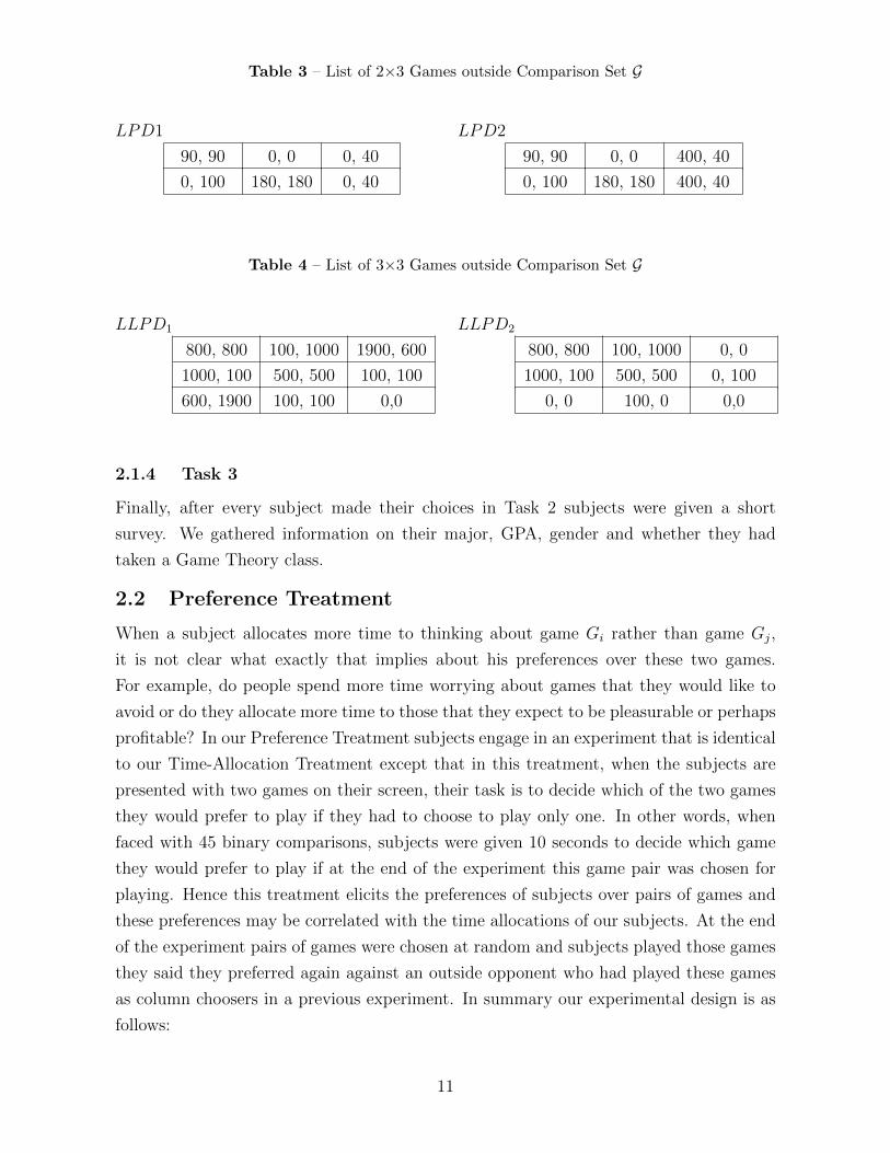
Table 3 – List of 2×3 Games outside Comparison Set G

LPD1

90, 90 0, 0 0, 40

0, 100 180, 180 0, 40

LPD2

90, 90 0, 0 400, 40

0, 100 180, 180 400, 40

Table 4 – List of 3×3 Games outside Comparison Set G

LLPD1

800, 800 100, 1000 1900, 600

1000, 100 500, 500 100, 100

600, 1900 100, 100 0,0

LLPD2

800, 800 100, 1000 0, 0

1000, 100 500, 500 0, 100

0, 0 100, 0 0,0

2.1.4 Task 3

Finally, after every subject made their choices in Task 2 subjects were given a short

survey. We gathered information on their major, GPA, gender and whether they had

taken a Game Theory class.

2.2 Preference Treatment

When a subject allocates more time to thinking about game Gi rather than game Gj,

it is not clear what exactly that implies about his preferences over these two games.

For example, do people spend more time worrying about games that they would like to

avoid or do they allocate more time to those that they expect to be pleasurable or perhaps

profitable? In our Preference Treatment subjects engage in an experiment that is identical

to our Time-Allocation Treatment except that in this treatment, when the subjects are

presented with two games on their screen, their task is to decide which of the two games

they would prefer to play if they had to choose to play only one. In other words, when

faced with 45 binary comparisons, subjects were given 10 seconds to decide which game

they would prefer to play if at the end of the experiment this game pair was chosen for

playing. Hence this treatment elicits the preferences of subjects over pairs of games and

these preferences may be correlated with the time allocations of our subjects. At the end

of the experiment pairs of games were chosen at random and subjects played those games

they said they preferred again against an outside opponent who had played these games

as column choosers in a previous experiment. In summary our experimental design is as

follows:

11

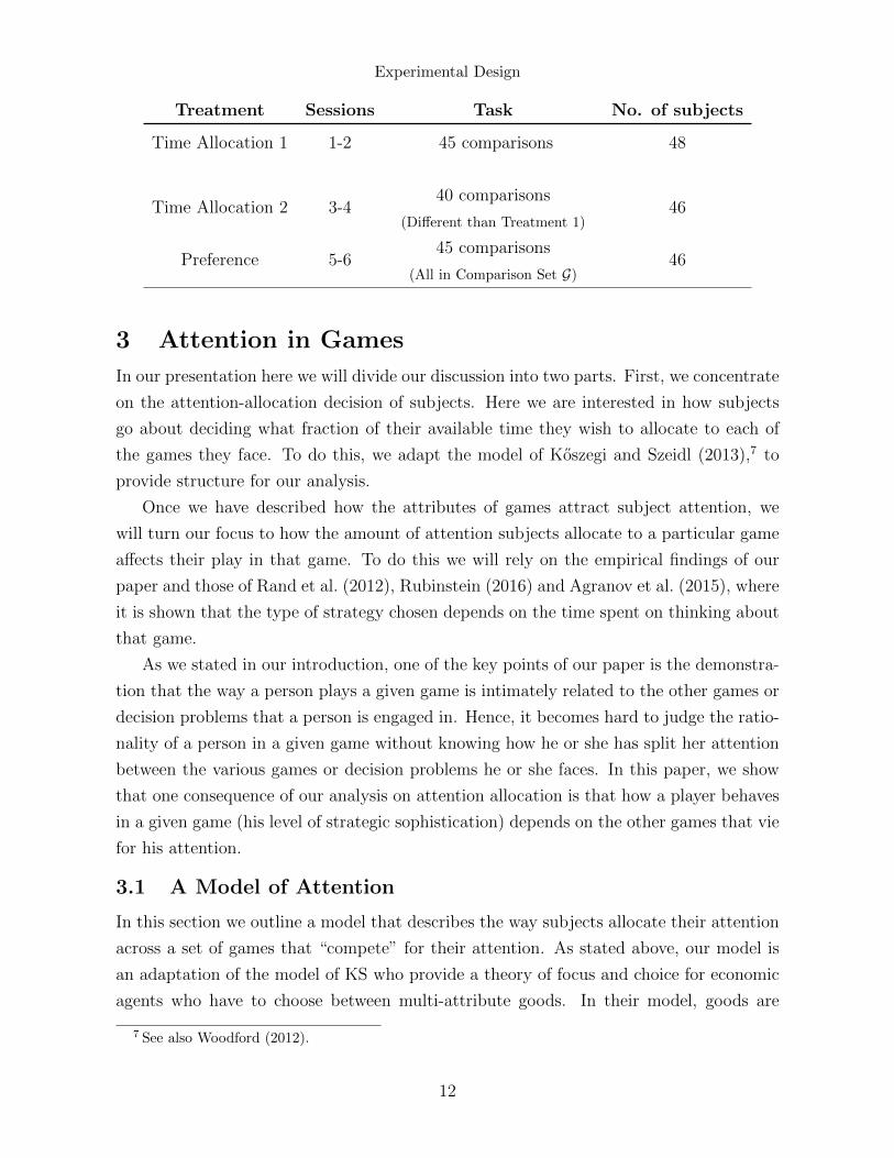
Experimental Design

Treatment Sessions Task No. of subjects

Time Allocation 1 1-2 45 comparisons 48

Time Allocation 2 3-440 comparisons

(Different than Treatment 1)46

Preference 5-645 comparisons

(All in Comparison Set G)46

3 Attention in Games

In our presentation here we will divide our discussion into two parts. First, we concentrate

on the attention-allocation decision of subjects. Here we are interested in how subjects

go about deciding what fraction of their available time they wish to allocate to each of

the games they face. To do this, we adapt the model of Koszegi and Szeidl (2013),7 to

provide structure for our analysis.

Once we have described how the attributes of games attract subject attention, we

will turn our focus to how the amount of attention subjects allocate to a particular game

affects their play in that game. To do this we will rely on the empirical findings of our

paper and those of Rand et al. (2012), Rubinstein (2016) and Agranov et al. (2015), where

it is shown that the type of strategy chosen depends on the time spent on thinking about

that game.

As we stated in our introduction, one of the key points of our paper is the demonstra-

tion that the way a person plays a given game is intimately related to the other games or

decision problems that a person is engaged in. Hence, it becomes hard to judge the ratio-

nality of a person in a given game without knowing how he or she has split her attention

between the various games or decision problems he or she faces. In this paper, we show

that one consequence of our analysis on attention allocation is that how a player behaves

in a given game (his level of strategic sophistication) depends on the other games that vie

for his attention.

3.1 A Model of Attention

In this section we outline a model that describes the way subjects allocate their attention

across a set of games that “compete” for their attention. As stated above, our model is

an adaptation of the model of KS who provide a theory of focus and choice for economic

agents who have to choose between multi-attribute goods. In their model, goods are

7 See also Woodford (2012).

12

described as bundles of attributes. More precisely, in their theory agents choose from a

finite set C ⊂ RK of K−dimensional consumption vectors, where each dimension repre-

sents an “attribute.” The consumption utility and welfare from a choice c = (c1, ......, cK)

is U(c) =∑K

k=1 u(ck). The key to their analysis, however, is a description of the fact that

while welfare is described by consumption utility, the good chosen is a function of what

they call its focus-weighted utility where focus or attention on a good is drawn to those

attributes that present the largest difference across goods. More precisely, subjects maxi-

mize U(c) =∑K

k=1 gkuk(ck), where gk = g(∆kC), ∆kC = (maxc∈C uk(ck)−minc∈C uk(ck)),

and g(·) is an increasing function. What this function says is that when looking across

bundles in C a consumer’s attention is drawn disproportionately to those attributes which

display the largest difference across the available goods. Large differences are given larger

weights via the gk(·) function. This focus on big differences leads people, as suggested by

KS to, for example, declare California preferable to Ohio as a place to live because of a

large difference in climate, while ignoring other attributes where the differences aren’t as

sizable. In KS the set of attributes is given exogenously.

In this paper, our subjects face a choice between matrix games each of which have

different attributes defined by their payoffs and their strategic attributes, i.e., the type of

game they are. For example, games differ in their maximum and minimum payoffs, by

how unequal their payoffs are, as well as the class of game they fall into, such as Pris-

oners’ Dilemma, Constant Sum, Battle of the Sexes or Pure coordination games.When

our subjects look across these games and have to decide on what fraction of their lim-

ited attention they want to pay to either game, they consider these attributes and the

differences in them across these games.

More precisely, games differ in their strategic and payoff attributes. To represent this

let a game Γ be described by its attribute vector a = (a1, ....aK , θ(Γ)), where the first K

attributes concern the payoffs in the game (i.e., maximum payoff, minimum payoff, how

inequitable are payoffs, etc.) and the second set of attributes relate to the type of game

the matrix represents denoted by a game-class variable θ(Γ). All strategic differences

between games will be represented by the class of game they fall into, i.e., whether they

are PC, BoS, CS, or PD games. In contemplating how much time or attention to

allocate to a particular game, the game-class variable θ(Γ) will function as an additive

constant that is added to the amount of time a subject will spend contemplating that

game as determined by its relative payoffs. For example, when comparing two games, if

game G1 is a Pure Coordination while game G2 is a Prisoners’ Dilemma game, then if

that distinction is recognized by the subjects and if they believe that PD games are more

13

difficult to contemplate than Pure Coordination games, then the time constant t(PD)

added to the attention allocated to the PD game will be greater than the time constant

added to the Pure Coordination game t(PC). Note that this game-class variable only

refers to the types of games we are comparing and not their payoffs.

Following KS, and restricting ourselves to comparisons of two matrix games at a time

(as is typically the case in our experiment), we define the focus-weighted attention score

of game Gi when it is compared to game Gj as T ij. More precisely, in our context we will

define T ij =∑K

k=1 gktk(aik) + t(θ(Gi)) as the attention score of game i when compared

to game j and likewise T ji =∑K

k=1 gktk(ajk) + t(θ(Gj)) for Gj’s attention score when

Gj is compared to game Gi. Here gk is the weight associated with attribute k given its

difference across the two games under investigation, while tk(ak) is the amount of time that

a game, containing attribute k of magnitude ak, adds to a subject’s contemplation time.

For example, as the largest payoff in a game matrix increases the game becomes more

attractive and attracts more of a player’s attention. The same is true as the worst payoff

in a game gets smaller since such a decrease lowers the value of the game and the worse

it gets the less one has to think about that game.8 Furthermore, as Rubinstein (2007)

and others have shown, games with large inequalities in payoffs also attract attention or

at least lead subjects to take longer before making a decision. The interesting aspect of

the KS model when applied to our analysis here is that the weight gk attached to each

payoff element, tk(aik), depends on how big is the difference in this attribute across the two

games. For simplicity, we define the fraction of time allocated to game Gi when compared

to game Gj as: α(i, j) = T ij

T ij+T ji . Obviously, α(j, i) = 1 − α(i, j). Note that this simply

says that the fraction of time allocated to game Gi is in proportion to its focus weighted

attraction score.

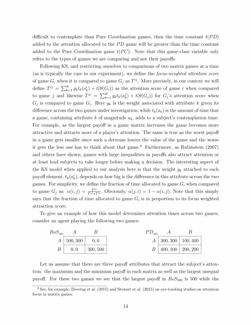
To give an example of how this model determines attention times across two games,

consider an agent playing the following two games:

BoS500 A B

A 500, 300 0, 0

B 0, 0 300, 500

PD300 A B

A 300, 300 100, 400

B 400, 100 200, 200

Let us assume that there are three payoff attributes that attract the subject’s atten-

tion: the maximum and the minimum payoff in each matrix as well as the largest unequal

payoff. For these two games we see that the largest payoff in BoS500 is 500 while the

8 See, for example, Devetag et al. (2015) and Stewart et al. (2015) on eye-tracking studies on attentionfocus in matrix games.

14

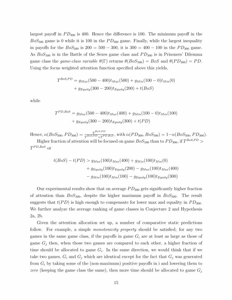
largest payoff in PD300 is 400. Hence the difference is 100. The minimum payoff in the

BoS500 game is 0 while it is 100 in the PD300 game. Finally, while the largest inequality

in payoffs for the BoS500 is 200 = 500 − 300, it is 300 = 400 − 100 in the PD300 game.

As BoS500 is in the Battle of the Sexes game class and PD300 is in Prisoners’ Dilemma

game class the game-class variable θ(Γ) returns θ(BoS500) = BoS and θ(PD300) = PD.

Using the focus weighted attention function specified above this yields,

TBoS,PD = gMax(500− 400)tMax(500) + gMin(100− 0)tMin(0)

+ gEquity(300− 200)tEquity(200) + t(BoS)

while

T PD,BoS = gMax(500− 400)tMax(400) + gMin(100− 0)tMin(100)

+ gEquity(300− 200)tEquity(300) + t(PD)

Hence, α(BoS500, PD300) = TBoS,PD

TBoS,PD

+TPD,BoS , with α(PD300, BoS500) = 1−α(BoS500, PD300).

Higher fraction of attention will be focused on gameBoS500 than to PD300, if TBoS,PD >

T PD,BoS or

t(BoS)− t(PD) > gMax(100)tMax(400) + gMin(100)tMin(0)

+ gEquity(100)tEquity(200)− gMax(100)tMax(400)

− gMin(100)tMin(100)− gEquity(100)tEquity(300)

Our experimental results show that on average PD300 gets significantly higher fraction

of attention than BoS500, despite the higher maximum payoff in BoS500. The result

suggests that t(PD) is high enough to compensate for lower max and equality in PD300.

We further analyze the average ranking of game classes in Conjecture 2 and Hypothesis

2a, 2b.

Given the attention allocation set up, a number of comparative static predictions

follow. For example, a simple monotonicity property should be satisfied; for any two

games in the same game class, if the payoffs in game Gi are at least as large as those of

game Gj then, when those two games are compared to each other, a higher fraction of

time should be allocated to game Gi. In the same direction, we would think that if we

take two games, Gi and Gj which are identical except for the fact that Gj was generated

from Gi by taking some of the (non-maximum) positive payoffs in i and lowering them to

zero (keeping the game class the same), then more time should be allocated to game Gj

15

since its minimum payoff has just been lowered making the difference in that minimum

even higher. Further, if we take two identical games, Gi and Gj that only differ in that

the payoffs in one cell of game Gi is unequal while those in game Gj are identical, then

we would expect a large fraction of time or attention to be allocated to game Gi. In

our analysis here we look at maximum inequality as the maximum difference between

payoffs in any cel of the matrix. In our later analysis we will restrict these inequalities to

equilibrium payoffs.

The predictions of our model stated above might contradict those of models who

consider that attention is drawn to more complex games where more computation is

needed to analyze them. That is, suppose one writes an algorithm to find an optimal

strategy in 2 × 2 matrix game. Then, if two games are in the same game class, it will

take the algorithm exactly the same time to find the solution. The time needed to return

an answer will depend on the class of the game, but will not depend on the magnitude

of payoffs. However, following our discussion on attributes, if the games are in the same

game class (the θ(Γ)’s are the same) then the attention focused on one game will be

strictly determined by the payoffs since they will affect each games’ attention score. In

the following section we state a set of conjectures that follow from our analysis. In our

Results Section we will reformulate these conjectures as hypotheses and use our data to

test them.

4 Conjectures

Most of our conjectures concern a comparison between the time allocated to either of two

games, games Gi and Gj when those games are compared to each other or to the same

set of alternative games, the Comparison Set G. To be more precise, let the set G contain

M games denoted G = {G1, G2, ..., GM}. In our experiment, as described above, a subject

is asked in a pair-wise fashion to allocate a fraction of time, X seconds, between game

Gi ∈ G and each of the other games in G. The conjectures below concern this allocation.

4.1 Interrelated Games

One consequence of the KS model when applied to our experiment is that the attention

allocated to a given game varies as we change the game or games it is compared to. There

is behavioral inter-game dependence.

Suppose, an agent focuses a fraction α(i, j) of his total attention on game Gi when it

is compared to game Gj. Now replace game Gj with game Gm, so that aj 6= am, i.e., the

payoff attributes of game Gj differ from those of game Gm. An agent is now comparing

game Gi and game Gm, and needs to decide how much attention to focus on game Gi,

16

(i.e., he must now determine α(i,m)). Given that the attributes of game Gj and game Gm

are not identical, aj 6= am, our focus-weighted attention score for game Gi when compared

to game Gj will differ from focus-weighted attention score for game Gi when compared

to game Gm, that is T ij 6= T im. Therefore, when we changed the opposing game, the

attention focus on the same game, game Gi, changed from α(i, j) to α(i,m), with α(i, j)

6= α(i,m). As a result, varying the second game in consideration from game Gj to game

Gm affected the attention focused on game Gi and hence, the behavior of our subjects in

game Gi. This yields a simple conjecture:

Conjecture 1 Interdependent Games: The way an agent behaves in a game is de-

pendent on the other game or games that agent is simultaneously engaged in.

We will restate this conjecture as a hypothesis and test it in the Results section of

this paper.

4.2 Strategic Attributes

When looking across types of games like Prisoners’ Dilemma games, Pure Coordination

games, Battle of the Sexes games or Constant Sum games, there may be a general view

that some of these games are easier to play than others and hence will attract less atten-

tion. In terms of our model, such games would imply a smaller game-class variable θ(Γ).

For example, it may be that across the four types of games just listed we might, on aver-

age, think that people would spend more of their time attending to Prisoners’ Dilemma

games as opposed to say Pure Coordination games. Likewise, since in Pure Coordination

games people’s interests are aligned while in the Battle of the Sexes games they are not,

we might expect more time to be allocated to the later than the former. It becomes

more difficult to conjecture about the relative contemplation times for our other games

since, while some, like the Battle of the Sexes game, contain equity issues, others, like the

Prisoners’ Dilemma, contain a trade-off between domination and efficiency. Which class

of games involve a larger additive constant, θ(Γ), is ultimately an empirical question but

our a priori expectations are summarized in the following conjecture.

Conjecture 2 Game Class Ordering: Let ¯PD, CS, ¯BoS, PC represent the mean

time allocated to all of the Prisoners’ Dilemma Games, Constant Sum Games, the Battle

of the Sexes Games and Pure Coordination Games, respectively, when compared to all

other games in G. We expect these times to be ordered as: ¯PD > CS > ¯BoS > PC.

As mentioned above, an algorithm or a trained game theorist performing our exper-

iment might conclude that once they can classify a game presented into a game class,

17

there would be no need to think more about it since strategically all games in that class

are equivalent. This would imply that the fraction of time allocated to such problems

when compared to any other game in the set G should be identical. In addition, if two

games in the same game class are compared directly, then the allocation of time should be

same – equal to 50%. However, given our model, if we have two games, Gi and Gj from

the same class of games, θ(Gi) = θ(Gj), then payoff attributes, ai and aj, will determine

the fraction of time allocated to each game, α(i, j). These considerations yield the two

conjectures stated below, and tested in the results section.

Conjecture 3 Game Class Irrelevance: For any two games Gi and Gj in the same

game class (i.e., both PD games, both CS games, etc.) the mean amount of time allocated

to each game should be identical for any comparisons made in the set G.

Conjecture 4 Within Class Payoff Irrelevance: For any two games Gi and Gj

in the same game class, when these games are compared to each other, each should be

allocated 50% of the available time no matter what their payoffs are.

4.3 Payoff Attributes

Some of the features of games that attract attention concern the game’s payoff attributes.

Lucrative games (defined appropriately) might cause you to think that the marginal ben-

efit of attending to that game is higher than a game with lower payoffs and hence might

attract attention. Games that look risky for various reasons, might also attract attention

as might games with negative or zero payoffs. The conjectures below are concerned with

these features. What we will be interested in investigating is how the time allocated to a

problem changes when we change one feature of the game’s payoffs.

However, since we are interested in ceteris paribus changes, we want to make sure that

the changes we introduce do not change the type of game being played. Hence, in several

of our conjectures we will require that whatever change we make in the game it remains

in the class of games we started with.

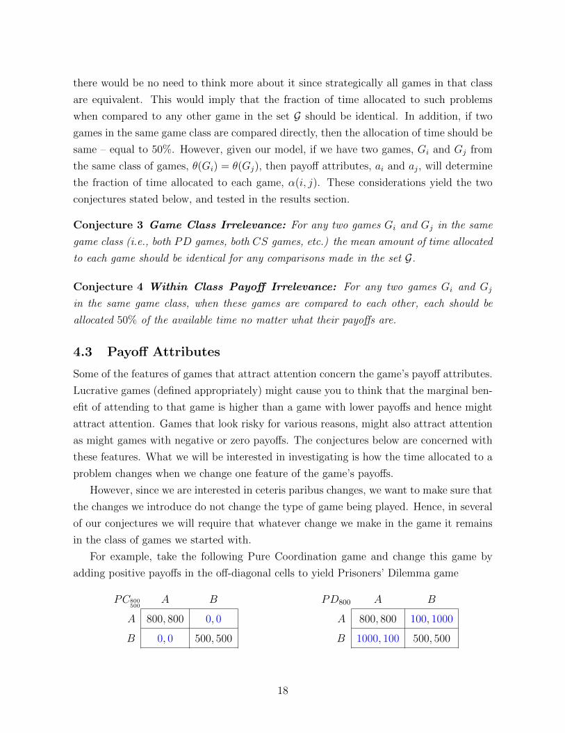
For example, take the following Pure Coordination game and change this game by

adding positive payoffs in the off-diagonal cells to yield Prisoners’ Dilemma game

PC800500

A B

A 800, 800 0, 0

B 0, 0 500, 500

PD800 A B

A 800, 800 100, 1000

B 1000, 100 500, 500

18

The second game is identical to the first with the exception that we have replaced

zero’s in PC800500

with some positive payoffs. However, note that PD800 is a Prisoners’

Dilemma game and hence outside of the game class we started with. As we will see later,

if we impose a monotonicity assumption that says that when two games are identical

except that one has strictly higher payoffs than the other, a subject will allocate more

time to the game with the higher payoffs, we may want to require that after the payoff

change the game still remains in the same class of games it started out in. We impose

this requirement because if the game type changes because of the payoff increase, subjects

may allocate more time to the second game not because the payoffs have increased, but

because they feel it is strategically more complicated. In order to avoid such confounds

we will, wherever possible, restrict such changes to games within a same game class.

Given our model in Section 3, if we have two games, Gi and Gj from the same class

of games so that θ(Gi) = θ(Gj), then payoff attributes, ai and aj, alone will determine

the fraction of time allocated to each game. Now, let payoffs in each cell of game Gi be

at least as large as in game Gj and strictly greater in at least one cell. When these two

games are compared to each other, the focus weighted attention score of Gi is going to be

greater than the focus weighted attention score of Gj.9 Therefore, α(i, j)—the fraction

of attention allocated to Gi—is going to be greater than α(j, i)—the fraction of attention

allocated to Gj. However, note that the model doesn’t necessarily predict a higher fraction

allocated to Gi than to Gj when both are compared to any Gm ∈ G. As we will see later,

this fact will be responsible for a large fraction of the inconsistencies in time allocation.

The discussion above yields the Monotonicity conjecture below.

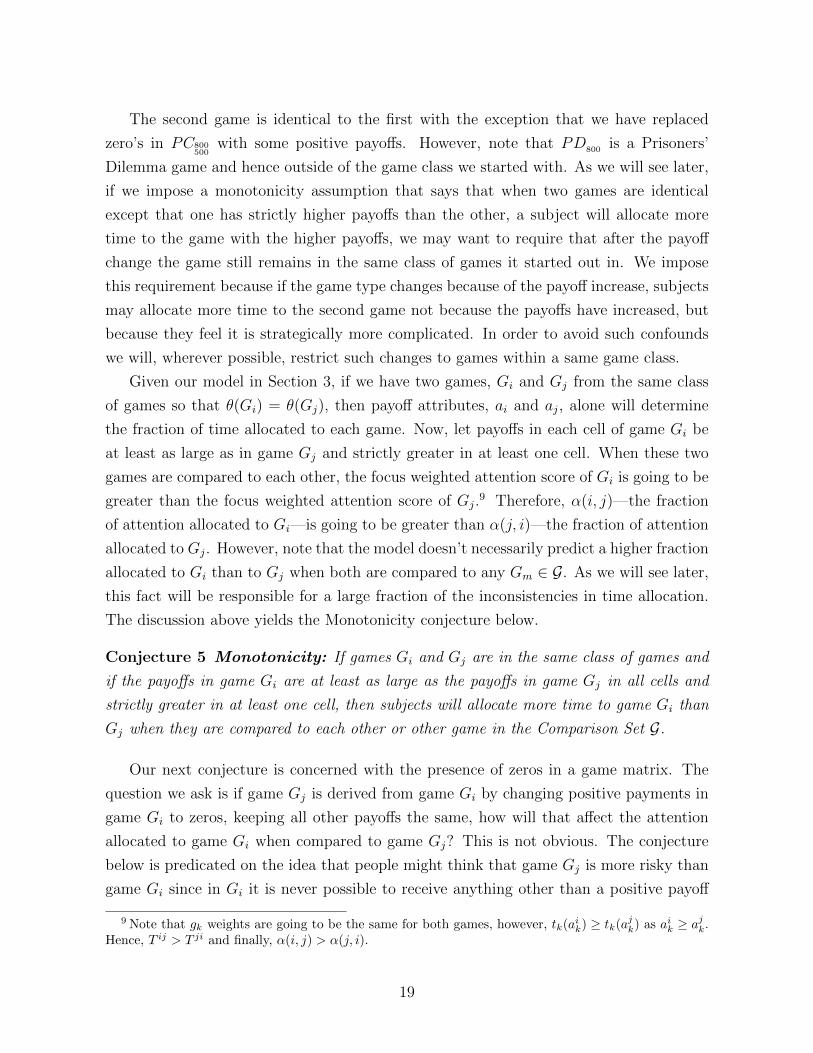
Conjecture 5 Monotonicity: If games Gi and Gj are in the same class of games and

if the payoffs in game Gi are at least as large as the payoffs in game Gj in all cells and

strictly greater in at least one cell, then subjects will allocate more time to game Gi than

Gj when they are compared to each other or other game in the Comparison Set G.

Our next conjecture is concerned with the presence of zeros in a game matrix. The

question we ask is if game Gj is derived from game Gi by changing positive payments in

game Gi to zeros, keeping all other payoffs the same, how will that affect the attention

allocated to game Gi when compared to game Gj? This is not obvious. The conjecture

below is predicated on the idea that people might think that game Gj is more risky than

game Gi since in Gi it is never possible to receive anything other than a positive payoff

9 Note that gk weights are going to be the same for both games, however, tk(aik) ≥ tk(ajk) as aik ≥ ajk.

Hence, T ij > T ji and finally, α(i, j) > α(j, i).

19

while in Gj it is. If zeros are considered scary payoffs then, in order to avoid receiving

them, subjects might want to think longer about game Gj before deciding what strategy

to choose. On the other hand, some people may think that because in creating game Gj

from game Gi we have made elements of Gi zero, game Gj has become simpler to analyze

and hence requires less time, i.e., there is less clutter in game Gi, and hence, it is easier

to process. There is no particular a priori reason to prefer one of these explanations to

the other. However, we can examine this statement using our model.

Suppose games Gi and Gj are from the same game class, θ(Gi) = θ(Gj), and let Gi

be identical to Gj except that all zeros in Gj are replaced by strictly positive payoffs,

keeping all other attributes unchanged. This will imply that the minimum of Gj is lower

than in Gi, while all other payoff and strategic attributes identical. Therefore, when

games Gi and Gj are compared to each other, the higher minimum in Gi will result in

higher focus weighted attention score for game Gi than the one for game Gj. Hence, more

attention will be payed to the game without zeros. However, note that if only some zeros

are replaced with positive payoffs but at least one of them is left unchanged that will

keep the minimums the same. Even though, the attention model doesn’t give a definitive

direction in this scenario, we are still able to test this case using our data.

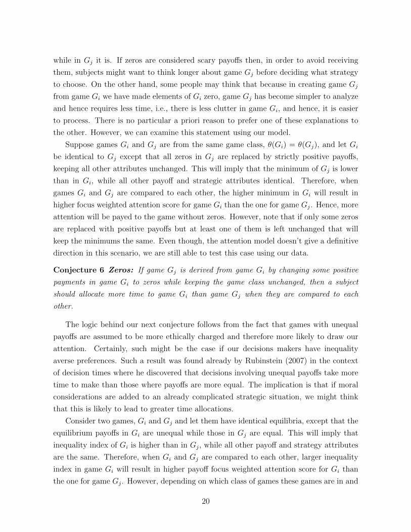
Conjecture 6 Zeros: If game Gj is derived from game Gi by changing some positive

payments in game Gi to zeros while keeping the game class unchanged, then a subject

should allocate more time to game Gi than game Gj when they are compared to each

other.

The logic behind our next conjecture follows from the fact that games with unequal

payoffs are assumed to be more ethically charged and therefore more likely to draw our

attention. Certainly, such might be the case if our decisions makers have inequality

averse preferences. Such a result was found already by Rubinstein (2007) in the context

of decision times where he discovered that decisions involving unequal payoffs take more

time to make than those where payoffs are more equal. The implication is that if moral

considerations are added to an already complicated strategic situation, we might think

that this is likely to lead to greater time allocations.

Consider two games, Gi and Gj and let them have identical equilibria, except that the

equilibrium payoffs in Gi are unequal while those in Gj are equal. This will imply that

inequality index of Gi is higher than in Gj, while all other payoff and strategy attributes

are the same. Therefore, when Gi and Gj are compared to each other, larger inequality

index in game Gi will result in higher payoff focus weighted attention score for Gi than

the one for game Gj. However, depending on which class of games these games are in and

20

the game class variable constants, more or less attention will be paid to the game with

unequal equilibrium payoffs.

Conjecture 7 Equity: If two games, Gi and Gj are identical and have identical equilib-

ria except that the equilibrium payoffs in game Gi are unequal while those in Gj are equal,

then a subject will allocate more time to game Gi with unequal payoffs when these games

are compared to each other.

Our final conjecture concerns complexity. One might think that one of the major

features of games that attract a player’s attention is their complexity. Unfortunately,

there is very little consensus as to what exactly makes a game complex and no commonly

agreed to standard. Despite this difficulty, there are situations where one might agree

that game Gi is more complex than game Gj and in our design we think we have such a

situation. More precisely, in those few instances where we expanded our games beyond

2×2 games to 3×3 games we did so by adding dominated strategies to one of our existing

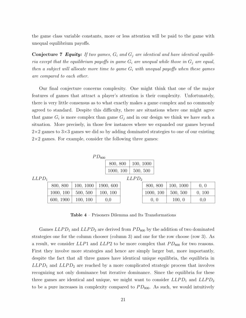
2×2 games. For example, consider the following three games:

PD800

800, 800 100, 1000

1000, 100 500, 500

LLPD1

800, 800 100, 1000 1900, 600

1000, 100 500, 500 100, 100

600, 1900 100, 100 0,0

LLPD2

800, 800 100, 1000 0, 0

1000, 100 500, 500 0, 100

0, 0 100, 0 0,0

Table 4 – Prisoners Dilemma and Its Transformations

Games LLPD1 and LLPD2 are derived from PD800 by the addition of two dominated

strategies one for the column chooser (column 3) and one for the row choose (row 3). As

a result, we consider LLP1 and LLP2 to be more complex that PD800 for two reasons.

First they involve more strategies and hence are simply larger but, more importantly,

despite the fact that all three games have identical unique equilibria, the equilibria in

LLPD1 and LLPD2 are reached by a more complicated strategic process that involves

recognizing not only dominance but iterative dominance. Since the equilibria for these

three games are identical and unique, we might want to consider LLPD1 and LLPD2

to be a pure increases in complexity compared to PD800. As such, we would intuitively

21

conclude that in a binary comparison between PD800 and LLPD1 or LLPD2, we would

expect more time to be allocated to the larger more complex games. This yields our last

conjecture.

Conjecture 8 If Game Gi is derived from game Gj by adding a strictly dominated strat-

egy to both the row and column player’s strategy set, then a subject will allocate more time

to game Gi than game Gj.

5 Results

In this Section we will start our discussion by investigating the conjectures presented

above. We split our analysis into two parts, one dealing with the question of the behavioral

inter-dependence of games and one on time allocation and consistency issues.

5.1 Interrelated Games

It is our claim in this paper that the time you allocate to thinking about any given game

depends on the other games you are simultaneously engaged in. However, since the way

you behave in a game depends on the amount of time you leave yourself to think about

it, the strategic and attention problems are intimately linked. In this section of the paper

we will investigate these two issues.

Hypothesis 1 Interdependent Games: 1. The time allocated to a given game is

independent of the other game a subject is facing. 2. The level of strategic sophistication

or the type of strategy chosen in a given game is independent of the time the subject

devoted to that game.

Given our data Hypothesis 1 is easily rejected. To give a simple illustration of how

the amount of time allocated to a game is affected by the other games a subject faces,

consider Figures 8a-d which present the mean amount of time allocated to the PC800,

BoS500, CS800, and PD300 games respectively as a function of the other games the subject

was engaged in.

<Figure 8>

Looking at Figure 8a first, we see there is a large variance in the amount of time

allocated to PC800 as we vary the other game that subjects who are engaged in this game

face. For example, on average subjects allocate less that 40% of their time to PC800 when

they also play PD800 while they allocate nearly 55% of their time to this game when also

22

facing PC500. For Figure 8b we see a similar pattern with subjects allocating close to 52%

of their time to that game when also facing the PC500 game but only around 40% to it

when simultaneously facing PD800. The same results hold in Figures 8c and 8d.

Table 5 presents the mean time allocated to each game in our Comparison Set G as

a function of the other game that game was paired with. Looking across each row, we

test the hypothesis that there is no difference in the fraction of time allocated to any

given game as a function of the “other game” the subject is playing which is what our

null hypothesis suggests. As we can see, while for some comparisons the difference is

insignificant, by and large there is a distinct pattern of the time allocated to a given game

depending on the other game a subject is simultaneously considering. This is supported

by a Friedman test that for any game in G we can reject the part one of the Hypothesis

1.

The second step in our analysis on interrelated games is to connect the time allocated

to a game type of strategy chosen. In other words, the question here is whether subjects

change the type of behavior they exhibit as the time allocated to a given game changes.

If this is true, and if the time allocated to a game depends on the other games a subject

faces, then we have demonstrated that we must consider the full set of games that a

person is playing before we can predict behavior in one isolated game.

We look for evidence of a function describing the relationship between contemplation

time and strategic choice except that given our design, we will have to content ourselves

with aggregate rather than individual level data. Figures 9a-c present such results.

<Figure 9>

In these figures we present decision time on the horizontal axis divided into two seg-

ments for those subjects spending less or more than the mean time of all subjects playing

this game. We put the fraction of subjects choosing strategy A in a given game on the

vertical axis. More simply, for any given game we compare the choices made by those sub-

jects who thought relatively little about the game (spent less than the mean time thinking

about it) to the choices of those who thought longer (more than the mean time).10

In Figure 9a, which looks at the CS400 game, the fraction of subjects choosing strategy

A who think relatively little about it is dramatically different from those who think a

longer time. For example, more than 76% of subjects who decide quickly in that game

choose A while, for those who think longer, this fraction drops to 43%. A similar, but

more dramatic pattern is found in Figure 9b for the PD300 game. Here the drop in the

10 The results are similar when we use the median instead of the mean.

23

fraction of subjects choosing strategy A (the cooperative strategy) is from 93% to 33%

indicating that quick choosers cooperate while slow choosers defect. Finally, in Figure 9c

we see that for some games choice is invariant with respect to decision time. Here, for the

game PC800500

we see that all subjects choose A no matter how long they think about the

game. Note that this is a coordination game with two Pareto-ranked equilibria one where

each subject receives a payoff of 800 and the other where the payoff is 500 (off diagonal

payoffs are 0). Choice in this game appears to be a no-brainer with all subjects seeing

that they should choose strategy.

The import of these figures for our thesis in this paper should be obvious. The time

allocated to a given game depends on the other game a subject is facing and choice in a

game typically depends on the time spent on it.

5.2 Attention Allocation

5.2.1 Preliminaries

In the remainder of this section we look in more depth at the time allocation problem.

Before we continue, it is important to consider the data we have. In total we ran four

sessions where sessions 1 and 2 we had subjects make 45 comparisons while sessions 3 and

4 we had them make 40 distinctly different ones. We ran sessions 3 and 4 to derive a set

of 11 games for which all games in the set were paired with each other. For 11 games in

the set

G = {PD300 , PD500 , PD800 , CS400 , CS500 , CS800 , BoS500 , BoS800 , PC500 , PC800 , Chance}we have a full set of 5511 comparisons such that each game in this set is compared to

every other game. This allows us to hold the comparison set constant and compare how

time is allocated between each game and every other game in set the G, thus, we are able

to make controlled comparisons.

For many of the comparisons we make we will concentrate on these 11 games. For

others we will focus on binary comparisons of games where either only one game is in Gor where both games are outside of G.

To make our comparisons we will use two metrics: mean time and fraction. The mean

time metric is exactly as it sounds. Here for any game Gi ∈ G we know that it was

compared to each of the ten games in the set G. We calculate the mean percentage of

time allocated to the game Gi over all ten comparisons in G. We do this for each of

the eleven games so each will have a mean score representing the mean fraction of time

allocated to this game when compared to each other game in G (Table 5).

11 All combination of two games out of eleven without replacement and order – C112 = 55.

24

The fraction metric records, for each comparison of games, what percentage of subjects

allocated strictly more than 50% of their time to a given game out of all subjects (we

exclude subjects who allocated exactly 50% to both games). For example, in Table 6

take PD800 and PD500 , both Prisoners’ Dilemma games. The number in the intersection

of PD800 row and PD500 column, 0.69, means that 69% of subjects allocated more than

50% to the first PD game and only 31% to the second game, when they were directly

compared to each other.

Tables 5 and 6 present these two metrics for all eleven games in the comparison set G.

One reads this table across the rows. For instance, in Table 5 which presents our mean

metric, we see that in the comparisons between PC800 and PC500 , on average, subjects

devoted 54.1% of their available time to the PC800 game and consequently, only 45.9%

to the PC500 game when these two games were compared directly. In other words, when

comparing PC800 to PC500 subjects felt they would like to spend more time contemplating

PC800 before making a choice. If we were to look at the same comparison in the Table 6,

where we present our fractions metric, we see that when the PC800vs PC500 comparison

was presented to subjects, 88% of them wanted to use more time thinking about PC800

than PC500 .

<Table 5> <Table 6>

5.2.2 Strategic Attributes

In discussing our conjectures we will discuss the impact of strategic considerations on time

allocation before we move on to the impact of payoffs. Since we investigate primarily four

basic types of games our first questions will concern whether more time was allocated to

certain types of games in aggregate. In other words, on average, was more time allocated

to PD games than PC games etc. when compared to other games in the set G. Here we

are taking the average across the set of games in G that each of our four types of games

were compared to, and then aggregating within each game class. This determines our

first null hypothesis:

Hypothesis 2a Game Class Ordering (mean): Let ¯PD, CS, ¯BoS, PC represent the

mean time allocated to all of the PD, CS, BoS, and the PC games when they are compared

with all other games in the set G. We test ¯PD = CS = ¯BoS = PC.

Hypothesis 2b Game Class Ordering (fraction): Let ˜PD, CS, ˜BoS, PC represent

the mean fraction of the PD, CS, BoS, and the PC games when they are compared with

all other games in the set G. We test ˜PD = CS = ˜BoS = PC.

25

<Table 7>

Table 7 presents data that allows us to test hypothesis 2a and 2b. It presents the mean

and the fraction metric for our classes of games and clearly indicates that both hypothesis

can be rejected. For example, it appears clear that as a class of games subjects allocated

more time to PD games (56.58%) followed by CS games (49.54%) then BoS games

(46.62%) and finally PC games (45.40%). A set of binary Wilcoxon signed-rank tests

indicates that these differences are statistically significant for all comparisons (p < 0.01)

except PC and BoS games where p > 0.05. A test of our null hypothesis, that the mean

attention time paid to games is equal across all game types, i.e., that ¯PD = PC = CS =¯BoS, is also rejected with p < 0.01 using a Friedman test.12

Similar results appear when we look at the fraction metric where PD games were

allocated more time on average, 78% of the time, compared to CS games (51%), BoS

games (34%), and PC games (26%). Again, a set of binary test of proportions indicate

that these mean fractions are significantly different except for PC and BoS classes. A

test of null hypothesis 2b that ˜PD = CS = ˜BoS = PC, is also rejected with p < 0.01.

Note that there is consistency between our two metrics in the sense that they order the

class of games in an identical manner as to which games attract more attention.

This result suggests that strategic factors are important in describing what types of

games attract attention. By and large, our subjects seem to be more concerned about

playing PD games as opposed to other types and least concerned about Pure Coordination

games. As we will see later, however, game class is not the only determining factor and

other, payoff-related, attributes of the game will also be important.

While Hypotheses 2a and 2b discuss attention issues aggregated across classes of

games, we can look within each game class and ask if there are differences in the at-

tention paid to games individually when compared to games in other classes. Here, of

course, since the games are from the same class, if subjects pay different amounts of at-

tention to them it must be because they have different payoff features. For example, let’s

consider the following hypothesis:

Hypothesis 3 Game Class Irrelevance: For any two games Gi and Gj in the same

game class (i.e., both PD games, both CS games, etc.) the mean amount of time allocated

to each game should be identical for any comparisons made in the set G.

12 The Friedman test is a non-parametric alternative to the one-way ANOVA with repeated measures.We will use Friedman test throughout this paper to test hypothesis involving more than two groups. Forone or two group analysis, we use Wilcoxon signed-rank test. In case of multiple hypothesis testing, asin Table 7, we use Bonferroni correction to adjust significance thresholds.

26

Hypothesis 3 is a way to look inside any class of games and look at how much attention

was allocated to each of these games when they were compared to games in the set Goutside their own class (i.e. we do not compare PD games with each other). We hypothesis

that the same attention will be paid to each of these games regardless their payoffs. As we

can see from Table 8, this hypothesis is rejected. For example, for PD games depending

on which PD game we look at, the mean fraction of time allocated to that game for all

out-of-class comparisons differs. While on average the mean percentage of time allocated

to PD800 when facing non-PD games in the set G was 58.52%, it was only 54.36% for

PD300 indicating that these two games, despite being PD games, were not viewed as

identical. Table 8 supports this result.

<Table 8>

Looking more broadly we see that for no class of games can we accept the null hypoth-

esis of equality of mean time allocations across games within the same class. This clearly

indicates that payoff features must be important when subjects decide how to allocate

attention across games.

If all games within a class are considered equivalent, we might expect that when they

are paired with each other in a binary comparison we should observe that each is allocated

an equal amount of time. For example, when comparing two PD games with different

payoffs it might be the case that since strategically they present identical trade-offs, a

subject might devote 50% to each no matter what their payoffs. These considerations

yield the following hypothesis.

Hypothesis 4 Game Class Payoff Irrelevance: For any two games Gi and Gj

in the same game class, when these games are compared to each other, each should be

allocated 50% of the available time no matter what their payoffs are.

<Table 9>

As we can see, from the Table 9, there is little support for Hypothesis 4. In Table 5

we present the mean time allocated to the Row game when paired with the Column game

along with the standard errors in parenthesis. What we are interested in is testing the

hypothesis that the mean in any cell is statistically different from 50%. As we can see, this

hypothesis is violated in almost all situations. For example, when BS800 is matched with

BoS8000

, subjects allocate 60.74% of their time to BoS800 which is significantly different

than the hypothesized 50% at the p < 0.01. Similarly, when BoS8000

is matched with

BoS800100

, it only attracts 42.78% of the time which is also significantly different than 50%

27

at the p < 0.01 level. The biggest exception to the rule is the class of Prisoners’ Dilemma

games where except for PD800 all other games seem to allocate a percentage of time

not significantly different to both games in any binary comparison. For example, when

PD300 is compared to PD8000

subjects allocated on average 48.67% to PD300 which is not

significantly different from 50% (p = 0.38).

In summary it appears that strategic considerations alone are not sufficient to explain

the attention that subjects pay to games. This indicates that subjects consider both

strategic as well as payoff features of games when deciding how much time to devote to

them. The implication therefore is that payoffs must matter. In the next section we

investigate exactly what it is about a game’s payoffs that attracts the subjects’ attention.

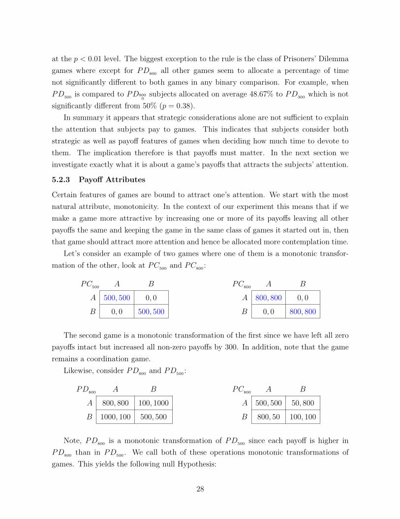
5.2.3 Payoff Attributes

Certain features of games are bound to attract one’s attention. We start with the most

natural attribute, monotonicity. In the context of our experiment this means that if we

make a game more attractive by increasing one or more of its payoffs leaving all other

payoffs the same and keeping the game in the same class of games it started out in, then

that game should attract more attention and hence be allocated more contemplation time.

Let’s consider an example of two games where one of them is a monotonic transfor-

mation of the other, look at PC500 and PC800 :

PC500 A B

A 500, 500 0, 0

B 0, 0 500, 500

PC800 A B

A 800, 800 0, 0

B 0, 0 800, 800

The second game is a monotonic transformation of the first since we have left all zero

payoffs intact but increased all non-zero payoffs by 300. In addition, note that the game

remains a coordination game.

Likewise, consider PD800 and PD500 :

PD800 A B

A 800, 800 100, 1000

B 1000, 100 500, 500

PC800 A B

A 500, 500 50, 800

B 800, 50 100, 100

Note, PD800 is a monotonic transformation of PD500 since each payoff is higher in

PD800 than in PD500 . We call both of these operations monotonic transformations of

games. This yields the following null Hypothesis:

28

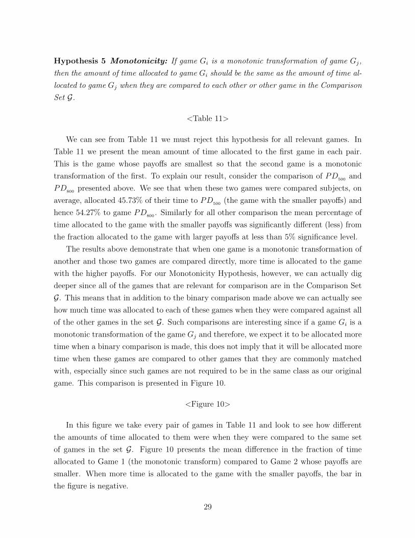
Hypothesis 5 Monotonicity: If game Gi is a monotonic transformation of game Gj,

then the amount of time allocated to game Gi should be the same as the amount of time al-

located to game Gj when they are compared to each other or other game in the Comparison

Set G.

<Table 11>

We can see from Table 11 we must reject this hypothesis for all relevant games. In

Table 11 we present the mean amount of time allocated to the first game in each pair.

This is the game whose payoffs are smallest so that the second game is a monotonic

transformation of the first. To explain our result, consider the comparison of PD500 and

PD800 presented above. We see that when these two games were compared subjects, on

average, allocated 45.73% of their time to PD500 (the game with the smaller payoffs) and

hence 54.27% to game PD800 . Similarly for all other comparison the mean percentage of

time allocated to the game with the smaller payoffs was significantly different (less) from

the fraction allocated to the game with larger payoffs at less than 5% significance level.

The results above demonstrate that when one game is a monotonic transformation of

another and those two games are compared directly, more time is allocated to the game

with the higher payoffs. For our Monotonicity Hypothesis, however, we can actually dig

deeper since all of the games that are relevant for comparison are in the Comparison Set

G. This means that in addition to the binary comparison made above we can actually see

how much time was allocated to each of these games when they were compared against all

of the other games in the set G. Such comparisons are interesting since if a game Gi is a

monotonic transformation of the game Gj and therefore, we expect it to be allocated more

time when a binary comparison is made, this does not imply that it will be allocated more

time when these games are compared to other games that they are commonly matched

with, especially since such games are not required to be in the same class as our original

game. This comparison is presented in Figure 10.

<Figure 10>

In this figure we take every pair of games in Table 11 and look to see how different

the amounts of time allocated to them were when they were compared to the same set

of games in the set G. Figure 10 presents the mean difference in the fraction of time

allocated to Game 1 (the monotonic transform) compared to Game 2 whose payoffs are

smaller. When more time is allocated to the game with the smaller payoffs, the bar in

the figure is negative.

29

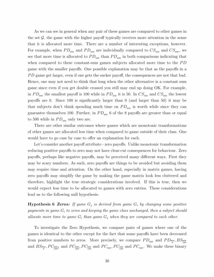
As we can see in general when any pair of these games are compared to other games in

the set G, the game with the higher payoff typically receives more attention in the sense

that it is allocated more time. There are a number of interesting exceptions, however.

For example, when PD800 and PD500 are individually compared to CS500 and CS800 , we

see that more time is allocated to PD500 than PD800 in both comparisons indicating that

when compared to these constant-sum games subjects allocated more time to the PD

game with the smaller payoffs. One possible explanation may be that as the payoffs in a

PD game get larger, even if one gets the sucker payoff, the consequences are not that bad.

Hence, one may not need to think that long when the other alternative is a constant sum

game since even if you get double crossed you still may end up doing OK. For example,

in PD800 the smallest payoff is 100 while in PD500 it is 50. In CS500 and CS800 the lowest

payoffs are 0. Since 100 is significantly larger than 0 (and larger than 50) it may be

that subjects don’t think spending much time on PD800 is worth while since they can

guarantee themselves 100. Further, in PD800 6 of the 8 payoffs are greater than or equal

to 500 while in PD500 only two are.

There are other similar outcomes where games which are monotonic transformations

of other games are allocated less time when compared to game outside of their class. One

would have to go case by case to offer an explanation for each.

Let’s consider another payoff attribute - zero payoffs. Unlike monotonic transformation

reducing positive payoffs to zero may not have clear-cut consequences for behaviour. Zero

payoffs, perhaps like negative payoffs, may be perceived many different ways. First they

may be scary numbers. As such, zero payoffs are things to be avoided but avoiding them

may require time and attention. On the other hand, especially in matrix games, having

zero payoffs may simplify the game by making the game matrix look less cluttered and

therefore, highlight the true strategic considerations involved. If this is true, then we

would expect less time to be allocated to games with zero entries. These considerations

lead us to the following null hypothesis.

Hypothesis 6 Zeros: If game Gj is derived from game Gi by changing some positive

payments in game Gi to zeros and keeping the game class unchanged, then a subject should

allocate more time to game Gi than game Gj when they are compared to each other.

To investigate the Zero Hypothesis, we compare pairs of games where one of the

games is identical to the other except for the fact that some payoffs have been decreased

from positive numbers to zeros. More precisely, we compare PD800 and PD8000, BS800

100

and BS8000, PC800

5001and PC800

500, PC800

100and PC800 , PC500

100and PC500 . We make these binary

30

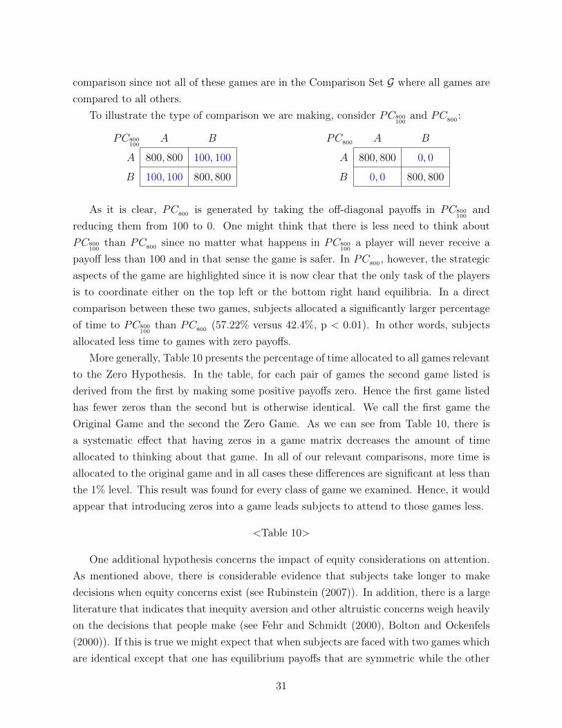
comparison since not all of these games are in the Comparison Set G where all games are

compared to all others.

To illustrate the type of comparison we are making, consider PC800100

and PC800 :

PC800100

A B

A 800, 800 100, 100

B 100, 100 800, 800

PC800 A B

A 800, 800 0, 0

B 0, 0 800, 800

As it is clear, PC800 is generated by taking the off-diagonal payoffs in PC800100

and

reducing them from 100 to 0. One might think that there is less need to think about

PC800100

than PC800 since no matter what happens in PC800100

a player will never receive a

payoff less than 100 and in that sense the game is safer. In PC800 , however, the strategic

aspects of the game are highlighted since it is now clear that the only task of the players

is to coordinate either on the top left or the bottom right hand equilibria. In a direct

comparison between these two games, subjects allocated a significantly larger percentage

of time to PC800100

than PC800 (57.22% versus 42.4%, p < 0.01). In other words, subjects

allocated less time to games with zero payoffs.

More generally, Table 10 presents the percentage of time allocated to all games relevant

to the Zero Hypothesis. In the table, for each pair of games the second game listed is

derived from the first by making some positive payoffs zero. Hence the first game listed

has fewer zeros than the second but is otherwise identical. We call the first game the

Original Game and the second the Zero Game. As we can see from Table 10, there is

a systematic effect that having zeros in a game matrix decreases the amount of time

allocated to thinking about that game. In all of our relevant comparisons, more time is

allocated to the original game and in all cases these differences are significant at less than

the 1% level. This result was found for every class of game we examined. Hence, it would

appear that introducing zeros into a game leads subjects to attend to those games less.

<Table 10>

One additional hypothesis concerns the impact of equity considerations on attention.

As mentioned above, there is considerable evidence that subjects take longer to make

decisions when equity concerns exist (see Rubinstein (2007)). In addition, there is a large

literature that indicates that inequity aversion and other altruistic concerns weigh heavily

on the decisions that people make (see Fehr and Schmidt (2000), Bolton and Ockenfels

(2000)). If this is true we might expect that when subjects are faced with two games which

are identical except that one has equilibrium payoffs that are symmetric while the other

31

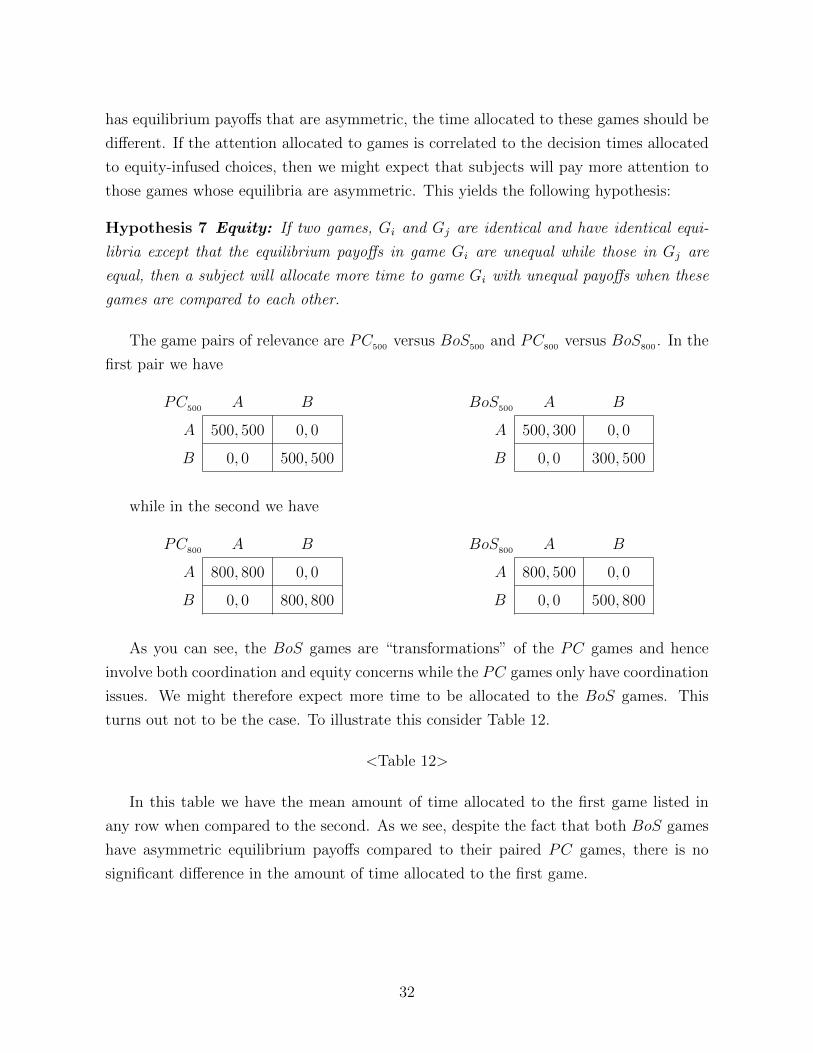
has equilibrium payoffs that are asymmetric, the time allocated to these games should be

different. If the attention allocated to games is correlated to the decision times allocated

to equity-infused choices, then we might expect that subjects will pay more attention to

those games whose equilibria are asymmetric. This yields the following hypothesis:

Hypothesis 7 Equity: If two games, Gi and Gj are identical and have identical equi-

libria except that the equilibrium payoffs in game Gi are unequal while those in Gj are

equal, then a subject will allocate more time to game Gi with unequal payoffs when these

games are compared to each other.

The game pairs of relevance are PC500 versus BoS500 and PC800 versus BoS800 . In the

first pair we have

PC500 A B

A 500, 500 0, 0

B 0, 0 500, 500

BoS500 A B

A 500, 300 0, 0

B 0, 0 300, 500

while in the second we have

PC800 A B

A 800, 800 0, 0

B 0, 0 800, 800

BoS800 A B

A 800, 500 0, 0

B 0, 0 500, 800

As you can see, the BoS games are “transformations” of the PC games and hence

involve both coordination and equity concerns while the PC games only have coordination

issues. We might therefore expect more time to be allocated to the BoS games. This

turns out not to be the case. To illustrate this consider Table 12.

<Table 12>

In this table we have the mean amount of time allocated to the first game listed in

any row when compared to the second. As we see, despite the fact that both BoS games

have asymmetric equilibrium payoffs compared to their paired PC games, there is no

significant difference in the amount of time allocated to the first game.

32

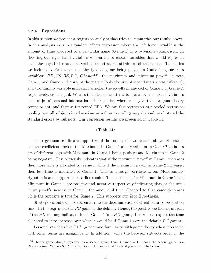
5.2.4 Regressions

In this section we present a regression analysis that tries to summarize our results above.

In this analysis we run a random effects regression where the left hand variable is the

amount of time allocated to a particular game (Game 1) in a two-game comparison. In

choosing our right hand variables we wanted to choose variables that would represent

both the payoff attributes as well as the strategic attributes of the games. To do this

we included variables such as the type of game being played in Game 1 (game class

variables: PD,CS,BS, PC, Chance13), the maximum and minimum payoffs in both

Game 1 and Game 2, the size of the matrix (only the size of second matrix was different),

and two dummy variable indicating whether the payoffs in any cell of Game 1 or Game 2,

respectively, are unequal. We also included some interactions of above mentioned variables

and subjects’ personal information: their gender, whether they’ve taken a game theory

course or not, and their self-reported GPA. We ran this regression as a pooled regression

pooling over all subjects in all sessions as well as over all game pairs and we clustered the

standard errors by subjects. Our regression results are presented in Table 14.

<Table 14>

The regression results are supportive of the conclusions we reached above. For exam-

ple, the coefficients before the Maximum in Game 1 and Maximum in Game 2 variables

are of different sign with Maximum in Game 1 being positive and Maximum in Game 2

being negative. This obviously indicates that if the maximum payoff in Game 1 increases

then more time is allocated to Game 1 while if the maximum payoff in Game 2 increases,

then less time is allocated to Game 1. This is a rough correlate to our Monotonicity

Hypothesis and supports our earlier results. The coefficient for Minimum in Game 1 and

Minimum in Game 1 are positive and negative respectively indicating that as the min-

imum payoffs increase in Game 1 the amount of time allocated to that game decreases

while the opposite is true for Game 2. This supports our Zero Hypothesis.

Strategic considerations also enter into the determination of attention or consideration

time. In the regression the PC game is the default. Hence, the positive coefficient in front

of the PD dummy indicates that if Game 1 is a PD game, then we can expect the time

allocated to it to increase over what it would be if Game 1 were the default PC games.

Personal variables like GPA, gender and familiarity with game theory when interacted

with other terms are insignificant. In addition, while the between subjects order of the

13 Chance game always appeared as a second game, thus, Chance = 1, means the second game is aChance game. While PD, CS, BoS, PC = 1, means that the first game is of that class.

33

comparisons was randomized, the subject order may still matter. However, we don’t find

an order effect in our experiment.

Finally note that our regression results comment on our last Conjecture concerning

complexity stated as the following hypothesis:

Hypothesis 8 If game Gi is derived from game Gj by adding a strictly dominated strategy

to both the row and column player’s strategy set, then a subject will allocate more time to

game Gi than game Gj.

Support for this hypothesis comes in two ways. First note that in the regression when

the number of cells in Game 2 increases, less time is allocated to Game 1. This clearly

suggests that larger game matrices strike our subjects as more complicated (even when

the added strategies are dominated) and hence deserving of more time. Further, as we

can see in Table 13 in a binary comparison between PD800 and either LLPD1 or LLPD2,

a higher fraction of time, 64.5 and 59.4, respectively, is allocated to the more complex

game. These differences are significant at the p < 0.01 level.

<Table 13>

Finally, it is important to point out we have only touched on this complicated issue of

complexity and certainly do not consider these results as definitive. The role of complexity

in the determination of attention is a complicated matter that should be dealt with in a

systematic manner.

5.3 Consistency

In this section of our paper we focus on whether the time-allocation decisions of our

subjects were consistent. While consistency of behavior has been studied with respect to

choice, it has rarely been looked with respect to attention. For example, in a two-good

commodity space, Choi et al. (2007) present subjects with a series of budget lines using a

very clever interface that allows them to test the GARP and WARP axioms. In our setting

we would be interested in discovering whether the subject choices, made both within and

across classes of games, are consistent. To do this we will specify a set of consistency

conditions that we think are reasonable and investigate whether our data supports them.

Our attention allocation function α(i, j) can be used to define a binary relation on Gcalled the “more worthy of attention” relationship such that if α(i, j) ≥ α(j, i) we would

say that game Gi is more worthy of attention in a binary comparison with game Gj. With

this notation we can specify four consistency conditions.

34

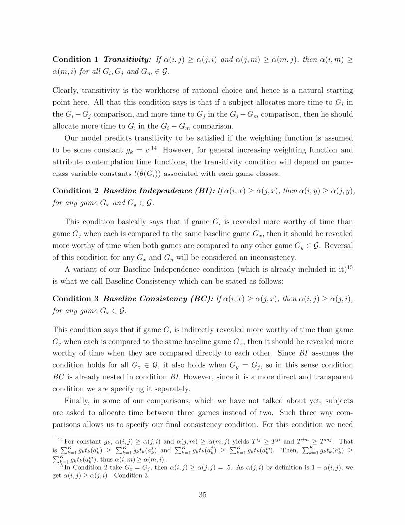
Condition 1 Transitivity: If α(i, j) ≥ α(j, i) and α(j,m) ≥ α(m, j), then α(i,m) ≥α(m, i) for all Gi, Gj and Gm ∈ G.

Clearly, transitivity is the workhorse of rational choice and hence is a natural starting

point here. All that this condition says is that if a subject allocates more time to Gi in

the Gi−Gj comparison, and more time to Gj in the Gj−Gm comparison, then he should

allocate more time to Gi in the Gi −Gm comparison.

Our model predicts transitivity to be satisfied if the weighting function is assumed

to be some constant gk = c.14 However, for general increasing weighting function and

attribute contemplation time functions, the transitivity condition will depend on game-

class variable constants t(θ(Gi)) associated with each game classes.

Condition 2 Baseline Independence (BI): If α(i, x) ≥ α(j, x), then α(i, y) ≥ α(j, y),

for any game Gx and Gy ∈ G.

This condition basically says that if game Gi is revealed more worthy of time than

game Gj when each is compared to the same baseline game Gx, then it should be revealed

more worthy of time when both games are compared to any other game Gy ∈ G. Reversal

of this condition for any Gx and Gy will be considered an inconsistency.

A variant of our Baseline Independence condition (which is already included in it)15

is what we call Baseline Consistency which can be stated as follows:

Condition 3 Baseline Consistency (BC): If α(i, x) ≥ α(j, x), then α(i, j) ≥ α(j, i),

for any game Gx ∈ G.

This condition says that if game Gi is indirectly revealed more worthy of time than game

Gj when each is compared to the same baseline game Gx, then it should be revealed more

worthy of time when they are compared directly to each other. Since BI assumes the

condition holds for all Gz ∈ G, it also holds when Gy = Gj, so in this sense condition

BC is already nested in condition BI. However, since it is a more direct and transparent

condition we are specifying it separately.

Finally, in some of our comparisons, which we have not talked about yet, subjects

are asked to allocate time between three games instead of two. Such three way com-

parisons allows us to specify our final consistency condition. For this condition we need

14 For constant gk, α(i, j) ≥ α(j, i) and α(j,m) ≥ α(m, j) yields T ij ≥ T ji and T jm ≥ Tmj . That

is∑K

k=1 gktk(aik) ≥∑K

k=1 gktk(ajk) and∑K

k=1 gktk(ajk) ≥∑K

k=1 gktk(amk ). Then,∑K

k=1 gktk(aik) ≥∑Kk=1 gktk(amk ), thus α(i,m) ≥ α(m, i).15 In Condition 2 take Gx = Gj , then α(i, j) ≥ α(j, j) = .5. As α(j, i) by definition is 1 − α(i, j), we

get α(i, j) ≥ α(j, i) - Condition 3.

35

the additional notation indicating that when three games Gi, Gj and Gk are compared

α(i, j, k) ≥ α(j, i, k) means that the decision maker allocates more time to game Gi than

game Gj when all three games are compared at the same time.

Condition 4 IIA: If α(i, j) ≥ α(j, i) then α(i, j, k) ≥ α(j, i, k).

This condition states that if game Gi is revealed more worthy of time than game

Gj when they are compared directly in a two-game comparison, then when we add an

additional game Gk and ask our subject to allocate time across these three games, game Gi

should still be revealed more worthy of time than game Gj in the three-game comparison.

Let us look at these consistency conditions one at a time.

5.3.1 Transitivity16

Our subjects prove themselves to be quite consistent in terms of transitivity. More pre-

cisely, transitivity is defined for every connected triple of games that we have data on.

In other words, we can check our transitivity condition for three games Gi, Gj and Gk if

in our experiment we have Gi compared to Gj, Gj compared to Gk and Gk compared to

Gi by the same subject. We call this cyclical comparison a triangle and in our analysis

below we will calculate the fraction of such triangles aggregated over all subjects for which

transitivity holds. There were 28 triangles in the comparisons used by subjects in Sessions

1 and 2 and 20 triangles in Sessions 3 and 4.

Our transitivity calculation is presented in Figure 11a were we look at all of our

subjects and portray the fraction of subjects making intransitive choices in the 28 triangles

they faced in Sessions 1 and 2 and the 20 triangles they faced in Sessions 3 and 4. As we

can see, over all sessions more than 79% of subjects exhibited either 0 or 1 intransitivity

while 91% exhibited strictly less than 3. A similar pattern exists when we look at the

individual sessions. For example, in Sessions 1 and 2, 92% present of subjects exhibited

strictly less that 3 intransitivities with no subject exhibiting more than 4. For Sessions 3

and 4 the corresponding percentage is 91%. In short, our more-worthy-than relationship

has proven itself to be largely transitive.

5.3.2 Baseline Independence (BI)

Transitivity is the easiest of our conditions to satisfy since all comparisons are direct

comparisons where the subject chooses between say games Gi and Gj directly then Gj

and Gk directly and then Gk and Gi. For our other conditions the comparisons are

16 In Appendix A, Figure 14 presents consistency results of our experimental data versus randomlygenerated data.

36

indirect and hence are more likely to exhibit inconsistencies. For example, consider our

BI Condition. Here we are saying that if Gi is shown to be more time worthy than Gj

when they are both compared to game Gx, then it should be more time worthy when

compared to any other game Gy in the set of all games G. This condition is more likely to

meet with inconsistencies since in the comparisons above, game Gy may be in a different

game class than game Gx so what is more time worthy when Gi and Gj are compared to

game Gx may not be considered as relevant when they are compared to game Gy.

This conjecture turns out to be true. In Figure 11b we present a histogram indicating

the frequency of violations of our Baseline Independence condition. The choices made

implied 46 comparisons where violations could be detected in Sessions 1 and 2 and 33

in Sessions 3 and 4; hence, when we detect a violation the maximum number of such

violations is 46 and 33 respectively. As we can see, there were an extremely large number

of violations of our Baseline Independence Condition. For example, the mean and median

number of violations per subjects were 10.7 and 10.5. Only 6 out of 92 subjects (6.5%)

had 1 or fewer violations compared to over 79% for our Intransitivity condition.

5.3.3 Baseline Consistency (BC)

We might expect that Baseline Consistency would be easier to satisfy than Baseline Inde-

pendence since under our consistency condition if game Gi is revealed to be more worthy

of time than Gj when both of them are compared to game Gx, then Gi should be revealed

to be more worthy of time when Gi and Gj are compared directly. BI requires that Gi be

revealed more worthy of time for all possible other comparisons that could be made. This

is a far more stringent condition since when we make these other comparisons we will be

comparing game Gi to a variety of games inside and outside of its own game class all with

varying payoff configurations while under BC we only compare it directly to game Gj.

Note that even Baseline Consistency is more difficult to satisfy than Transitivity as BC

implies Transitivity but the converse is not true.17

As we can see in Figure 11c, our results are consistent with this intuition. For exam-

ple, only 20 subjects (21%) exhibited 1 or fewer violations of our Baseline Consistency

condition as compared to 79% for Transitivity and 6.25% for Independence. 36 subjects

(38%) exhibited 5 or more violations of Consistency compared to 1 (1%) who violated

Transitivity that many times and 43 (89%) who had that many violations of Independence.

17 Consider three games: Gi, Gj and Gk. Suppose pair Gi, Gk gets 40-60%, Gj , Gk gets 30-70% andfinally, Gi, Gj gets 25-75%. We have a set {(k, i), (k, j), (j, i)} which satisfies transitivity, however, itviolates consistency as game Gi appears more time valuable than Gj when compared to Gk, nevertheless,when compared directly to game Gi is allocated less time than game Gj .

37

5.3.4 Independence of Irrelevant Alternatives (IIA)

Our final consistency measurement concerns our IIA condition. Given our design there

were only 24 subjects in Session 1 that were presented with the type of three-game com-

parisons that will allow us to test our IIA condition. For each subject there were 13

relevant comparisons or situations where we could detect an IIA violation. As Figure

11d indicates, violations were the rule rather than the exception. For example, out of 13

possible situations the mean and median number of violations per subject was 3.9 and 4

respectively. The modal number of violations was 5 with 3 out of 24 subjects violating

IIA in 9 out of 13 occasions. 3 subjects had no violations.

In summary, while our subjects appeared to have made consistent choices when viewed

through the lens of transitivity, they appeared to fail to do so when the consistency

requirements were strengthened or at least became more indirect. As we suggested, it is

difficult for our subjects to maintain consistency when the comparisons they face span

different types of games with varying payoffs. While transitivity is likely to be violated

when goods are multidimensional we found that to the contrary transitivity was the

consistence condition that fared well.

<Figure 11>

5.4 Preference Treatments

When a subject decides to pay more attention to some game rather than other, what

does that imply about his preferences over these games? Are preferences and attention

correlated and if so in what direction?

All of these questions will be answered in this section of our paper. To do this we will

use the data generated by our Preference Treatment and compare it to the data generated

by our Time-Allocation Treatment. We will proceed by asking how the time allocated to a

game is related to the preference for playing that game. To compare behavior in our time

allocation and preference treatments we merely need to compare the fraction of subjects

who allocate more time to a game when compared to another with the fraction of subjects

stating they prefer that game. In other words, if in our Time Allocation Treatment we

define a binary variable to take the value of 1 when a subject allocates more time to game

Gi than game Gj and 0 otherwise then we can compare this variable to one that takes a

value of 1 when a subject states he prefers game Gi over game Gj and zero otherwise in

our Preference Treatment. We will exploit this feature repeatedly.

38

5.4.1 Preferences and Attention

In this subsection we try to infer what it means when a subject decides to spend more

time thinking about game Gi rather than game Gj. An inference that suggests that the

subject prefers game Gi to game Gj may be faulty. For example, the revealed preference

statement “Since Johnny spends all day thinking about his little league game at the

expense of his school work he must enjoy it more than school work” might ignore the fact

that little Johnny may actually hate baseball and is only obsessing about it because it is

a source of great anxiety as he may fear humiliation in front of his friends.

To get a look into this relationship we took each of the 11 games in the Comparison

set G minus the Chance game and looked at both the time that was allocated to this game

when compared to the other 9 games and also how often this game was preferred to the

game it was paired with. For each game we then split the game comparisons into four

subsets depending on the time allocated and the preference stated in each comparison.

To explain this more fully, take one of the 10 games in G minus Chance game, say

PD800 . This game was compared to each of the other 9 games in G. Take all subjects who

made these comparisons and for any given comparison look at the fraction of subjects

who allocated more time to PD800 than the other game in the comparison. Also calculate

the fraction of times subjects stated that they preferred PD800 in this comparison. Now

divide the outcomes of all such comparisons into four subsets: those outcomes where

PD800 was simultaneously allocated more time by at least 50% of subjects and was also

preferred by more than 50% of them, those where the opposite was true, i.e., more than

50% of the subjects allocated less time to this game and it was preferred by less than 50%

of subjects, and the two mixed cases where subjects either allocated more time to a game

but liked it less or allocated less time on a game and liked it more (note that because

we did not run a within-subjects design, we can not make these calculations subject by

subject but must aggregate across all subjects).

<Figure 12>

Figure 12 presents the results of this calculation for each game in the Comparison Set

G. As we can see, preferences and time allocation appear to be highly correlated in the

sense that most of the observations are arrayed along the diagonal indicating a positive

association between time allocation and preference. Looking at the games in each cell is

interesting. For example, PD games heavily occupy the upper left hand cell in Figure

12 indicating that PD games attract a lot of attention and also are preferred to their

comparison games. More precisely, for the PD800 game in 9 of the 9 comparisons it faced

39

more than 50% of subjects allocated more time to it and also stated they preferred it to

the game it was being compared to. This was also true for 8 of the 9 comparison made

for the PD500 game and 6 of the 9 made for the PD300 game. The opposite seems to be

true of PC games. For example, there are no PC500 entries in the upper left hand cell

of Figure 12 while 7 such entries occur in the bottom right-hand cell where more than

50% of subjects both allocated less time to PC500 and listed it as their least preferred

alternative. For PC800 we see that in 6 of 9 comparisons more than 50% of subjects listed

it as their top alternative yet in three of those comparisons more than 50% of subjects

allocated less than 50% of their time to it.

Games in the bottom right-hand cell are interesting since these are games which appear

to be unpopular and to which subjects choose to allocate less time to. For example, BoS500

and CS500 seem to be the least popular games in the sense that in 6 of 9 companions they

were each the least preferred choice of more than 50% of subjects and more than 50% of

subjects also allocated less time to it. As stated above, one might think that unpleasant

games might attract more attention (remember little Johnny) but this seems not to be the

case. Some of this can be explained by looking at payoffs. For example, PC500 is a pure

coordination game with payoffs of 500 each for subjects in the upper left and lower right

hand cells and zeros on the off diagonals. PC800 is the same game but with payoffs of 800.

As can be seen, possibly because of its lower payoffs, PC500 was an unpopular game and

also one that people decided to allocate less time to while PC800 was popular (preferred

in 6 of 9 comparisons) but not paid much attend to (in only 3 of 9 comparisons did more

than 50% of subjects allocate more time to it). There are relatively few mixed cases,

i.e., entries in the off-diagonal cells in Figure 12, where subjects either prefer a game but

allocate less time to it or do not prefer the game but spend a lot of time thinking about

it.

The punch line of Figure 12, therefore, appears to be that the time allocated to a

problem (or at least whether more (or less) than 50% of subjects allocate more time to it

in any comparison) is a sign that subjects actually prefer (or do not prefer) playing that

game rather than its comparison game.

Finally we ask how consistent were our subjects’ preferences across games in the sense

that if they stated a preference for game Gi over game Gj and to game Gj over game

Gk, did they also state a preference for game Gi over game Gk? This is exactly the same

transitivity question asked of our subjects with respect to their time allocation. As Figure

13 suggests, our subjects were far more consistent in their time allocations than they were

with respect to their preferences.

40

<Figure 13>

For example, the fraction of subjects violating transitivity less than 2% (4%) of the

time is far greater in the Attention Treatment than in the Preference Treatment. More

precisely, while 47.3% (66.7%) of subjects in the Attention Treatment violated transitiv-

ity less than 2% (4%), 6.5% (17.4%) violated transitivity that often in the Preference

Treatment. The distribution of intransitivities in the Attention Treatment first-order

stochastically dominates that of the Preference Treatment.

6 Conclusions

In this paper we examine the question of why do people behave in games the way they

do. In answering this question we have extended the set of concerns players have when

playing a game to include attentional issues which derive from the fact that people do

not play games in isolation but rather have to share their attention across a set of games.

The choices that people make in one game viewed in isolation can only be understood by

including the full inter-game or general equilibrium problem they face.

We have posited a two step decision process in games. First is an attentional stage

which prescribes how much time players should allocate to any given game when they are

faced with several games to play simultaneously. To help us structure our thinking about

this stage, we adopted KS model of focus-weight attention. After this problem is solved

then our subjects need to decide how to behave given the time they have allocated.

With respect to the first, the attentional problem, by presenting subjects with pairs

of games and asking them to allocate a fraction of decision time to them, we have tried

to examine what features of games attract the most attention and hence are played in a

more sophisticated way. As might be expected, subjects devote time to thinking about

games as a function of their payoffs and their strategic properties in comparison to the

other games they are simultaneously playing. As payoffs in a given game increase, ceteris

paribus, subjects allocate more time to it. As the number of zeros in a game increase,

subjects tend to want to think less about it. Finally, while payoffs impact attention the

strategic aspects of the games being compared also matter in the sense that people tend,

on average, to allocate more time to Prisoners’ Dilemma games followed by Constant Sum

games and the Battle of the Sexes game and, finally, Pure Coordination games.

In terms of behavior, our results strongly support the idea that how people play in any

given game depends on the other game (or games) they are simultaneously dividing their

attention among. This can help explain why some people can look very sophisticated

in their behavior in some parts of their lives but rather naive in others since, given the

41

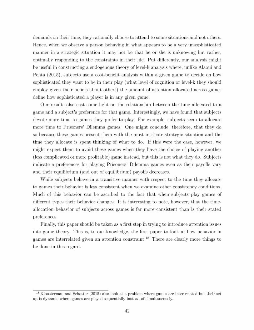
demands on their time, they rationally choose to attend to some situations and not others.

Hence, when we observe a person behaving in what appears to be a very unsophisticated

manner in a strategic situation it may not be that he or she is unknowing but rather,

optimally responding to the constraints in their life. Put differently, our analysis might

be useful in constructing a endogenous theory of level-k analysis where, unlike Alaoui and

Penta (2015), subjects use a cost-benefit analysis within a given game to decide on how

sophisticated they want to be in their play (what level of cognition or level-k they should

employ given their beliefs about others) the amount of attention allocated across games

define how sophisticated a player is in any given game.

Our results also cast some light on the relationship between the time allocated to a

game and a subject’s preference for that game. Interestingly, we have found that subjects

devote more time to games they prefer to play. For example, subjects seem to allocate

more time to Prisoners’ Dilemma games. One might conclude, therefore, that they do

so because these games present them with the most intricate strategic situation and the

time they allocate is spent thinking of what to do. If this were the case, however, we

might expect them to avoid these games when they have the choice of playing another

(less complicated or more profitable) game instead, but this is not what they do. Subjects

indicate a preferences for playing Prisoners’ Dilemma games even as their payoffs vary

and their equilibrium (and out of equilibrium) payoffs decreases.

While subjects behave in a transitive manner with respect to the time they allocate

to games their behavior is less consistent when we examine other consistency conditions.

Much of this behavior can be ascribed to the fact that when subjects play games of

different types their behavior changes. It is interesting to note, however, that the time-

allocation behavior of subjects across games is far more consistent than is their stated

preferences.

Finally, this paper should be taken as a first step in trying to introduce attention issues

into game theory. This is, to our knowledge, the first paper to look at how behavior in

games are interrelated given an attention constraint.18 There are clearly more things to

be done in this regard.

18 Kloosterman and Schotter (2015) also look at a problem where games are inter related but their setup is dynamic where games are played sequentially instead of simultaneously.

42

References

Agranov, Marina, Andrew Caplin, and Chloe Tergiman, “Naive play and the

process of choice in guessing games,” Journal of the Economic Science Association,

2015, 1 (2), 146–157.

Alaoui, Larbi and Antonio Penta, “Endogenous depth of reasoning,” The Review of

Economic Studies, 2015, pp. 1–37.

and , “Endogenous Depth of Reasoning and Response Time, with an application to

the Attention-Allocation Task,” 2016.

Andersson, Ola, Jim Ingebretsen Carlson, Erik Wengstrom et al., “Differences

Attract: An Experimental Study of Focusing in Economic Choice,” Department of

Economics, Lund Universtiy Working Papers, 2016, (2016: 15).

Arad, Ayala and Ariel Rubinstein, “The 11–20 money request game: a level-k rea-

soning study,” The American Economic Review, 2012, 102 (7), 3561–3573.

Bear, Adam and David G Rand, “Intuition, deliberation, and the evolution of coop-

eration,” Proceedings of the National Academy of Sciences, 2016, 113 (4), 936–941.

Bednar, Jenna, Yan Chen, Tracy Xiao Liu, and Scott Page, “Behavioral spillovers

and cognitive load in multiple games: An experimental study,” Games and Economic

Behavior, 2012, 74 (1), 12–31.

Bolton, Gary E and Axel Ockenfels, “ERC: A theory of equity, reciprocity, and

competition,” American economic review, 2000, pp. 166–193.

Bordalo, Pedro, Nicola Gennaioli, and Andrei Shleifer, “Salience and consumer

choice,” Technical Report, National Bureau of Economic Research 2012.

, , and , “Competition for Attention,” Review of Economic Studies, 2016, 83 (2),

481–513.

Bushong, Benjamin, Matthew Rabin, and Joshua Schwartzstein, “A model of

relative thinking,” Technical Report, working paper 2015.

Choi, Syngjoo, “A cognitive hierarchy model of learning in networks,” Review of Eco-

nomic Design, 2012, 16 (2-3), 215–250.

43

, Raymond Fisman, Douglas Gale, and Shachar Kariv, “Consistency and het-

erogeneity of individual behavior under uncertainty,” The American economic review,

2007, 97 (5), 1921–1938.

Cunningham, Tom, “Comparisons and choice,” Unpublished Manuscript, Harvard Uni-

versity, 2011.

Devetag, Giovanna, Sibilla Di Guida, and Luca Polonio, “An eye-tracking study

of feature-based choice in one-shot games,” Experimental Economics, 2015, pp. 1–25.

Fehr, Ernst and Klaus M Schmidt, “Fairness, incentives, and contractual choices,”

European Economic Review, 2000, 44 (4), 1057–1068.

Fischbacher, Urs, “z-Tree: Zurich toolbox for ready-made economic experiments,” Ex-

perimental economics, 2007, 10 (2), 171–178.

Gabaix, Xavier, “A sparsity-based model of bounded rationality,” Technical Report,

National Bureau of Economic Research 2011.

Kessler, Judd, Hannu Kivimaki, and Muriel Niederle, “Generosity Over Time,”

Technical Report, Working Paper 2015.

Kloosterman, Andrew and Andrew Schotter, “Dynamic Games with Complemen-

tarities: An Experiment,” 2015.

Koszegi, Botond and Adam Szeidl, “A model of focusing in economic choice,” The

Quarterly Journal of Economics, 2013, 128 (1), 53–104.

Lindner, Florian and Matthias Sutter, “Level-k reasoning and time pressure in the

11–20 money request game,” Economics Letters, 2013, 120 (3), 542–545.

Rand, David G, Joshua D Greene, and Martin A Nowak, “Spontaneous giving

and calculated greed,” Nature, 2012, 489 (7416), 427–430.

Recalde, Marıa P, Arno Riedl, and Lise Vesterlund, “Error prone inference from

response time: The case of intuitive generosity,” 2014.

Rubinstein, Ariel, “Instinctive and cognitive reasoning: a study of response times,”

The Economic Journal, 2007, 117 (523), 1243–1259.

, “A typology of players: Between instinctive and contemplative,” The Quarterly Jour-

nal of Economics, 2016, 131 (2), 859–890.

44

Savikhin, Anya C and Roman M Sheremeta, “Simultaneous decision-making in

competitive and cooperative environments,” Economic Inquiry, 2013, 51 (2), 1311–

1323.

Schotter, Andrew and Isabel Trevino, “Is response time predictive of choice? An

experimental study of threshold strategies,” Technical Report, WZB Discussion Paper

2014.

Stewart, Neil, Simon Gachter, Takao Noguchi, and Timothy L Mullett, “Eye

movements in strategic choice,” Journal of Behavioral Decision Making, 2015, 29 (2-3),

137–156.

Woodford, Michael, “Inattentive Valuation and Reference-Dependent Choice,” Unpub-

lished, 2012.

45

Appendix

A Figures

Figure 6 – Sample Screen

Figure 7 – Sample Chance Screen

46

Figure 8 – Average Time Allocation

40

45

50

55

60

PC500 BS800 BS500 CS500 CS400 CS800 Chance PD800 PD500 PD300

Games from Comparison Set

Aver

age

Tim

e

Time Allocation: PC800 vs

(a)

40

45

50

55

PC500 PC800 BS800 CS500 CS400 CS800 Chance PD800 PD500 PD300

Games from Comparison Set

Aver

age

Tim

e

Time Allocation: BS500 vs

(b)

40

45

50

55

PC500 PC800 BS800 BS500 CS500 CS400 Chance PD800 PD500 PD300

Games from Comparison Set

Aver

age

Tim

e

Time Allocation: CS400 vs

(c)

45

50

55

60

PC500 PC800 BS800 BS500 CS500 CS400 CS800 Chance PD800 PD500

Games from Comparison Set

Aver

age

Tim

e

Time Allocation: PD300 vs

(d)

Figure 9 – Time Taken and Strategy Relation

43

76

Less than Mean Time More than Mean Time

Per

centa

ge

of

Subje

cts

Pla

yin

g A

CS400

(a)

33

93

Less than Mean Time More than Mean Time

Perc

enta

ge o

f S

ubje

cts

Pla

yin

g A

PD300

(b)

100

Less than Mean Time More than Mean Time

Perc

enta

ge o

f S

ubje

cts

Pla

yin

g A

PC800 500−0

(c)

47

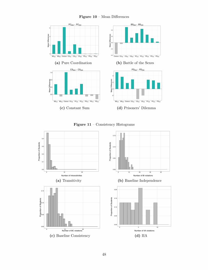
Figure 10 – Mean Differences

0

4

8

12

BS500 BS800 Chance CS400 CS500 CS800 PD300 PD500 PD800

Me

an

Diffe

ren

ce

s

PC800 − PC500

(a) Pure Coordination

-5.0

-2.5

0.0

2.5

5.0

Chance CS400 CS500 CS800 PC500 PC800 PD300 PD500 PD800

Me

an

Diffe

ren

ce

s

BS800 − BS500

(b) Battle of the Sexes

0.0

2.5

5.0

7.5

BS500 BS800 Chance CS400 PC500 PC800 PD300 PD500 PD800

Me

an

Diffe

ren

ce

s

CS800 − CS500

(c) Constant Sum

-2

0

2

4

BS500 BS800 Chance CS400 CS500 CS800 PC500 PC800 PD800

Me

an

Diffe

ren

ce

s

PD800 − PD500

(d) Prisoners’ Dilemma

Figure 11 – Consistency Histograms

0.0

0.1

0.2

0.3

0.4

0 10 20

Number of Intransitivities

Pro

port

ion o

f S

tudents

(a) Transitivity

0.00

0.05

0.10

0.15

0 10 20 30 40

Number of BI violations

Pro

port

ion o

f S

tudents

(b) Baseline Independence

0.00

0.05

0.10

0.15

0 10 20Number of BC violations

Pro

port

ion o

f S

tudents

(c) Baseline Consistency

0.00

0.05

0.10

0.15

0.20

0 5 10

Number of IIA violations

Pro

port

ion o

f S

tudents

(d) IIA

48

Fig

ure

12

–T

ime

All

oca

tion

and

Pre

fere

nce

sC

omb

ined

Pre

fere

nce

Tre

atm

ent

More

than

50L

ess

than

50

PC

800,PC

800,PC

800;

BoS

800;

BoS

800,BoS

800,BoS

800;

BoS

500;

More

CS

800,CS

800,CS

800;

CS

500,CS

500;

than

50CS

400,CS

400,CS

400,CS

400,CS

400;

CS

800,CS

800;

PD

800,PD

800,PD

800,PD

800,PD

800,PD

800,PD

800,PD

800,PD

800;

CS

400;

PD

500,PD

500,PD

500,PD

500,PD

500,PD

500,PD

500,PD

500;

Mea

nPD

300,PD

300,PD

300,PD

300,PD

300,PD

300;

Tre

atm

ent

PC

500,PC

500;

PC

500,PC

500,PC

500,PC

500,PC

500,PC

500,PC

500;

PC

800,PC

800,PC

800;

PC

800,PC

800,PC

800;

BoS

800;

BoS

800,BoS

800,BoS

800,BoS

800;

Less

BoS

500;

BoS

500,BoS

500,BoS

500,BoS

500,BoS

500,BoS

500,BoS

500;

than

50CS

800;

CS

500,CS

500,CS

500,CS

500,CS

500,CS

500,CS

500;

PD

300;

CS

800,CS

800,CS

800;

CS

400,CS

400,CS

400;

PD

500;

PD

300,PD

300;

49

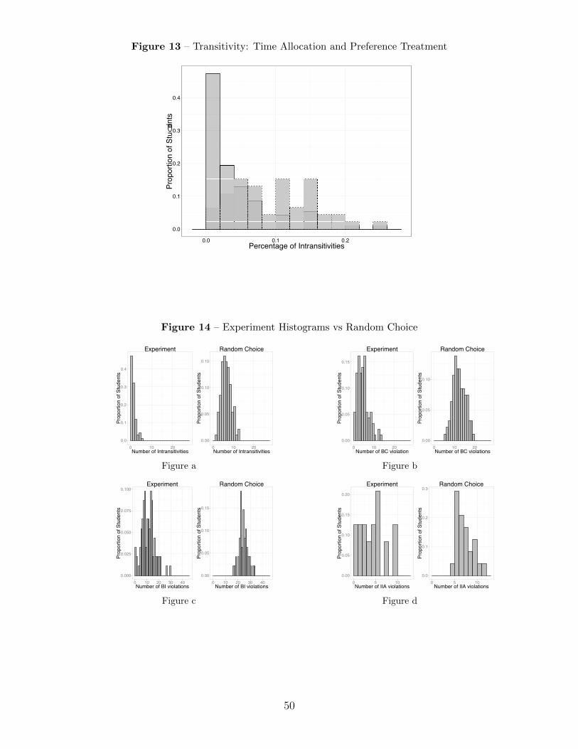
Figure 13 – Transitivity: Time Allocation and Preference Treatment

0.0

0.1

0.2

0.3

0.4

0.0 0.1 0.2Percentage of Intransitivities

Pro

port

ion o

f S

tudents

Figure 14 – Experiment Histograms vs Random Choice

0.0

0.1

0.2

0.3

0.4

0 10 20Number of Intransitivities

Pro

port

ion o

f S

tudents

Experiment

0.00

0.05

0.10

0.15

0 10 20Number of Intransitivities

Pro

port

ion o

f S

tudents

Random Choice

Figure a

0.00

0.05

0.10

0.15

0 10 20Number of BC violation

Pro

port

ion o

f S

tudents

Experiment

0.00

0.05

0.10

0 10 20Number of BC violations

Pro

port

ion o

f S

tudents

Random Choice

Figure b

0.000

0.025

0.050

0.075

0.100

0 10 20 30 40Number of BI violations

Pro

port

ion o

f S

tudents

Experiment

0.00

0.05

0.10

0.15

0 10 20 30 40Number of BI violations

Pro

port

ion o

f S

tudents

Random Choice

Figure c

0.00

0.05

0.10

0.15

0.20

0 5 10Number of IIA violations

Pro

port

ion o

f S

tudents

Experiment

0.0

0.1

0.2

0.3

0 5 10Number of IIA violations

Pro

port

ion o

f S

tudents

Random Choice

Figure d

50

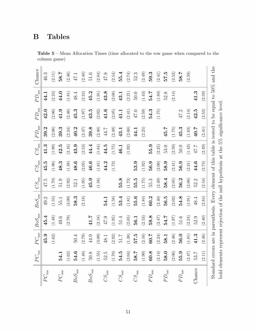
B Tables

Table 5 – Mean Allocation Times (time allocated to the row game when compared to thecolumn game)

PC

500

PC

800

BoS

800

BoS

500

CS

500

CS

800

CS

400

PD

800

PD

500

PD

300

Chan

ce

PC

500

45.9

45.4

49.2

47.5

45.5

41.3

39.2

42.0

44.1

46.3

(1.6

2)(1

.48)

(1.5

5)(1

.70)

(1.9

6)

(1.9

9)

(2.0

6)

(2.0

6)

(2.2

4)

(2.1

1)

PC

800

54.1

49.6

55.1

51.9

48.3

42.5

39.3

41.9

44.0

58.7

(1.6

2)(2

.79)

(3.0

9)(2

.92)

(1.3

8)

(2.1

6)

(2.2

4)

(2.4

6)

(1.8

1)

(2.4

6)

BoS

800

54.6

50.4

58.3

52.1

48.6

43.9

40.2

45.3

48.4

47.1

(1.4

8)(2

.79)

(2.1

8)(1

.95)

(2.0

5)

(2.5

3)

(2.4

7)

(1.9

7)

(2.2

4)

(2.4

0)

BoS

500

50.8

44.9

41.7

45.9

46.6

44.4

39.8

43.5

45.2

51.6

(1.5

5)(3

.09)

(2.1

8)(1

.58)

(1.8

1)

(1.8

4)

(2.4

0)

(2.0

2)

(1.9

1)

(2.8

4)

CS

500

52.5

48.1

47.9

54.1

44.2

44.5

44.7

41.6

43.8

47.8

(1.7

0)(2

.92)

(1.9

5)(1

.58)

(1.7

3)

(1.7

5)

(2.4

9)

(2.0

5)

(2.0

8)

(2.5

4)

CS

800

54.5

51.7

51.4

53.4

55.8

46.1

43.1

41.1

43.1

55.4

(2.0

4)(1

.38)

(2.0

5)(1

.81)

(1.7

3)

(1.9

2)

(2.0

0)

(2.4

1)

(2.2

1)

(2.7

4)

CS

400

58.7

57.5

56.1

55.6

55.5

53.9

44.1

47.0

50.0

52.3

(1.9

9)(2

.16)

(2.5

3)(1

.84)

(1.7

5)

(1.9

2)

(2.2

5)

(2.5

9)

(1.4

3)

(2.4

9)

PD

800

60.8

60.7

59.8

60.2

55.3

56.9

55.9

54.3

54.7

59.3

(2.1

4)(2

.24)

(2.4

7)(2

.40)

(2.4

9)

(2.0

0)

(2.2

5)

(1.7

5)

(1.8

3)

(2.4

1)

PD

500

58.0

58.1

54.7

56.5

58.4

58.9

53.0

45.7

52.8

57.5

(2.0

6)(2

.46)

(1.9

7)(2

.02)

(2.0

5)

(2.4

1)

(2.5

9)

(1.7

5)

(2.1

4)

(2.5

3)

PD

300

55.9

56.0

51.6

54.8

56.2

56.9

50.0

45.3

47.2

58.7

(2.4

7)(1

.81)

(2.2

4)(1

.91)

(2.0

8)

(2.2

1)

(1.4

3)

(1.8

3)

(2.1

4)

(2.5

9)

Chan

ce53

.741.3

52.9

48.4

52.2

44.6

47.7

40.7

42.5

41.3

(2.1

1)(2

.46)

(2.4

0)(2

.84)

(2.5

4)

(2.7

4)

(2.4

9)

(2.4

1)

(2.5

3)

(2.5

9)

Sta

ndar

der

rors

are

inpar

enth

esis

.E

very

elem

ent

ofth

ista

ble

iste

sted

tob

eeq

ual

to50

%an

dth

e

bol

del

emen

tsre

pre

sent

reje

ctio

nof

the

null

hyp

othes

isat

the

5%si

gnifi

cance

leve

l.

51

Table 6 – Percentage (share of students who allocated strictly greater than 50% to the rowgame)

PC

500

PC

800

BoS

800

BoS

500

CS

500

CS

800

CS

400

PD

800

PD

500

PD

300

Chan

ce

PC

500

0.1

20.2

20.

410.1

70.2

90.0

70.1

20.1

50.2

60.

43

(0.0

8)(0

.08)

(0.1

0)(0

.09)

(0.0

9)

(0.0

5)

(0.0

6)

(0.0

6)

(0.0

8)

(0.0

8)

PC

800

0.8

80.

350.

530.

520.

410.1

30.2

00.1

30.2

70.7

8

(0.0

8)(0

.09)

(0.0

9)(0

.10)

(0.1

2)

(0.0

6)

(0.0

7)

(0.0

6)

(0.0

7)

(0.0

8)

BoS

800

0.7

80.

650.9

40.

500.

360.3

00.1

30.1

80.

320.

39

(0.0

8)(0

.09)

(0.0

6)(0

.10)

(0.0

9)

(0.0

8)

(0.0

6)

(0.0

7)

(0.0

8)

(0.0

8)

BoS

500

0.59

0.47

0.0

60.2

40.2

70.1

70.0

70.2

10.2

80.

58

(0.1

0)(0

.09)

(0.0

6)(0

.09)

(0.0

9)

(0.0

7)

(0.0

5)

(0.0

8)

(0.0

8)

(0.1

0)

CS

500

0.8

30.

480.

500.7

60.1

40.2

10.

330.1

50.2

30.

35

(0.0

9)(0

.10)

(0.1

0)(0

.09)

(0.0

7)

(0.0

8)

(0.0

8)

(0.0

6)

(0.0

8)

(0.0

9)

CS

800

0.7

10.

590.

640.7

30.8

60.2

90.2

50.1

90.2

10.

67

(0.0

85)

(0.1

2)(0

.09)

(0.0

9)(0

.07)

(0.0

9)

(0.0

8)

(0.0

8)

(0.0

8)

(0.0

9)

CS

400

0.9

30.8

70.7

00.8

30.7

90.7

10.

310.2

70.

550.

49

(0.0

5)(0

.06)

(0.0

8)(0

.07)

(0.0

8)

(0.0

9)

(0.0

9)

(0.0

9)

(0.1

1)

(0.0

8)

PD

800

0.8

80.8

00.8

70.9

30.

670.7

50.

690.

690.8

10.7

7

(0.0

6)(0

.07)

(0.0

6)(0

.047

)(0

.08)

(0.0

8)

(0.0

9)

(0.0

9)

(0.0

8)

(0.0

7)

PD

500

0.8

50.8

70.8

20.7

90.8

50.8

10.7

30.

310.

710.8

4

(0.0

6)(0

.06)

(0.0

7)(0

.08)

(0.0

6)

(0.0

8)

(0.0

9)

(0.0

9)

(0.1

0)

(0.0

7)

PD

300

0.7

40.7

30.

680.7

20.7

70.7

90.

450.1

90.

290.7

7

(0.0

8)(0

.07)

(0.0

8)(0

.08)

(0.0

8)

(0.0

8)

(0.1

1)

(0.0

8)

(0.1

0)

(0.0

7)

Chan

ce0.

570.2

20.

610.

420.

650.

330.

510.2

30.1

60.2

3

(0.0

8)(0

.08)

(0.0

8)(0

.10)

(0.0

9)

(0.0

9)

(0.0

8)

(0.0

7)

(0.0

7)

(0.0

7)

Sta

ndar

der

rors

are

inpar

enth

esis

.E

very

elem

ent

ofth

ista

ble

iste

sted

tob

eeq

ual

to0.

50an

dth

e

bol

del

emen

tsre

pre

sent

reje

ctio

nof

the

null

hyp

othes

isat

the

5%si

gnifi

cance

leve

l.

52

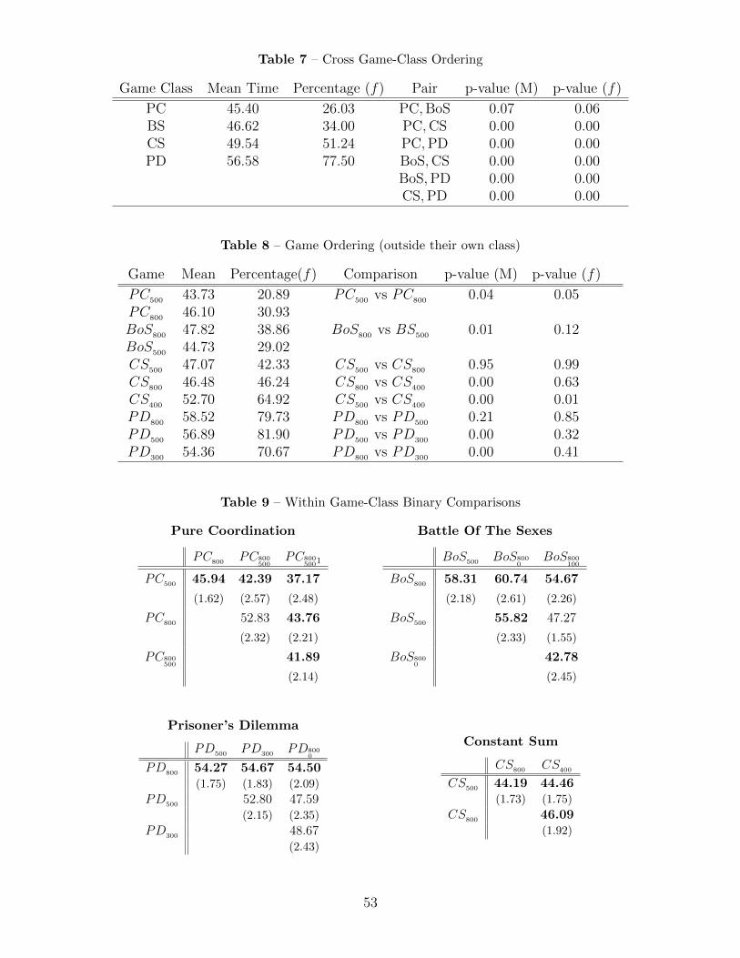
Table 7 – Cross Game-Class Ordering

Game Class Mean Time Percentage (f) Pair p-value (M) p-value (f)

PC 45.40 26.03 PC,BoS 0.07 0.06BS 46.62 34.00 PC,CS 0.00 0.00CS 49.54 51.24 PC,PD 0.00 0.00PD 56.58 77.50 BoS,CS 0.00 0.00

BoS,PD 0.00 0.00CS,PD 0.00 0.00

Table 8 – Game Ordering (outside their own class)

Game Mean Percentage(f) Comparison p-value (M) p-value (f)

PC500 43.73 20.89 PC500 vs PC800 0.04 0.05PC800 46.10 30.93BoS800 47.82 38.86 BoS800 vs BS500 0.01 0.12BoS500 44.73 29.02CS500 47.07 42.33 CS500 vs CS800 0.95 0.99CS800 46.48 46.24 CS800 vs CS400 0.00 0.63CS400 52.70 64.92 CS500 vs CS400 0.00 0.01PD800 58.52 79.73 PD800 vs PD500 0.21 0.85PD500 56.89 81.90 PD500 vs PD300 0.00 0.32PD300 54.36 70.67 PD800 vs PD300 0.00 0.41

Table 9 – Within Game-Class Binary Comparisons

Pure Coordination

PC800 PC800500

PC8005001

PC500 45.94 42.39 37.17

(1.62) (2.57) (2.48)

PC800 52.83 43.76

(2.32) (2.21)

PC800500

41.89

(2.14)

Battle Of The Sexes

BoS500 BoS8000

BoS800100

BoS800 58.31 60.74 54.67

(2.18) (2.61) (2.26)

BoS500 55.82 47.27

(2.33) (1.55)

BoS8000

42.78

(2.45)

Prisoner’s Dilemma

PD500 PD300 PD8000

PD800 54.27 54.67 54.50(1.75) (1.83) (2.09)

PD500 52.80 47.59(2.15) (2.35)

PD300 48.67(2.43)

Constant Sum

CS800 CS400

CS500 44.19 44.46(1.73) (1.75)

CS800 46.09(1.92)

53

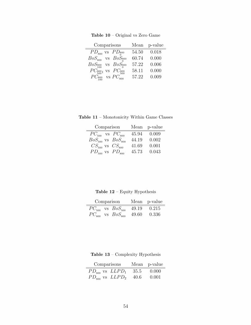
Table 10 – Original vs Zero Game

Comparisons Mean p-value

PD800 vs PD8000

54.50 0.018

BoS800 vs BoS8000

60.74 0.000

BoS800100

vs BoS8000

57.22 0.006

PC8005001

vs PC800500

58.11 0.000

PC800100

vs PC800 57.22 0.009

Table 11 – Monotonicity Within Game Classes

Comparison Mean p-value

PC500 vs PC800 45.94 0.009BoS500 vs BoS800 44.19 0.002CS500 vs CS800 41.69 0.001PD500 vs PD800 45.73 0.043

Table 12 – Equity Hypothesis

Comparison Mean p-value

PC500 vs BoS500 49.19 0.215PC800 vs BoS800 49.60 0.336

Table 13 – Complexity Hypothesis

Comparisons Mean p-value

PD800 vs LLPD1 35.5 0.000PD800 vs LLPD2 40.6 0.001

54

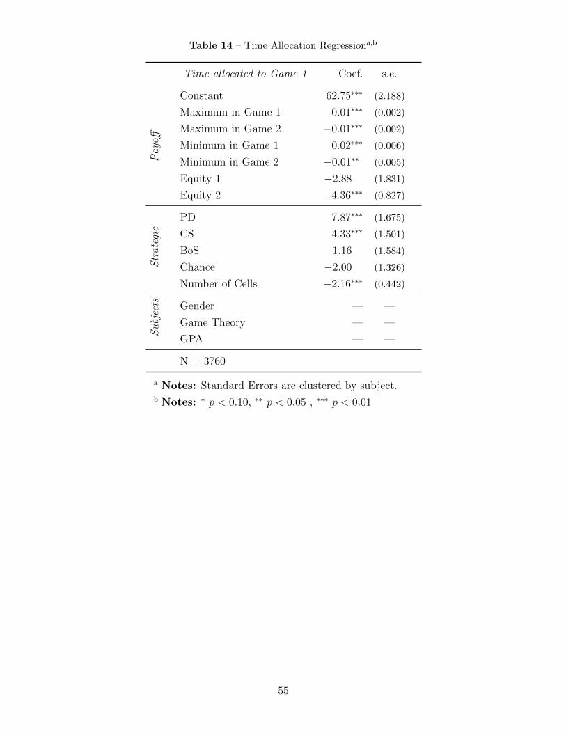
Table 14 – Time Allocation Regressiona,b

Time allocated to Game 1 Coef. s.e.

Constant 62.75∗∗∗ (2.188)

Pay

off

Maximum in Game 1 0.01∗∗∗ (0.002)

Maximum in Game 2 −0.01∗∗∗ (0.002)

Minimum in Game 1 0.02∗∗∗ (0.006)

Minimum in Game 2 −0.01∗∗ (0.005)

Equity 1 −2.88 (1.831)

Equity 2 −4.36∗∗∗ (0.827)

Str

ateg

ic

PD 7.87∗∗∗ (1.675)

CS 4.33∗∗∗ (1.501)

BoS 1.16 (1.584)

Chance −2.00 (1.326)

Number of Cells −2.16∗∗∗ (0.442)

Su

bjec

ts Gender — —

Game Theory — —

GPA — —

N = 3760

a Notes: Standard Errors are clustered by subject.b Notes: ∗ p < 0.10, ∗∗ p < 0.05 , ∗∗∗ p < 0.01

55

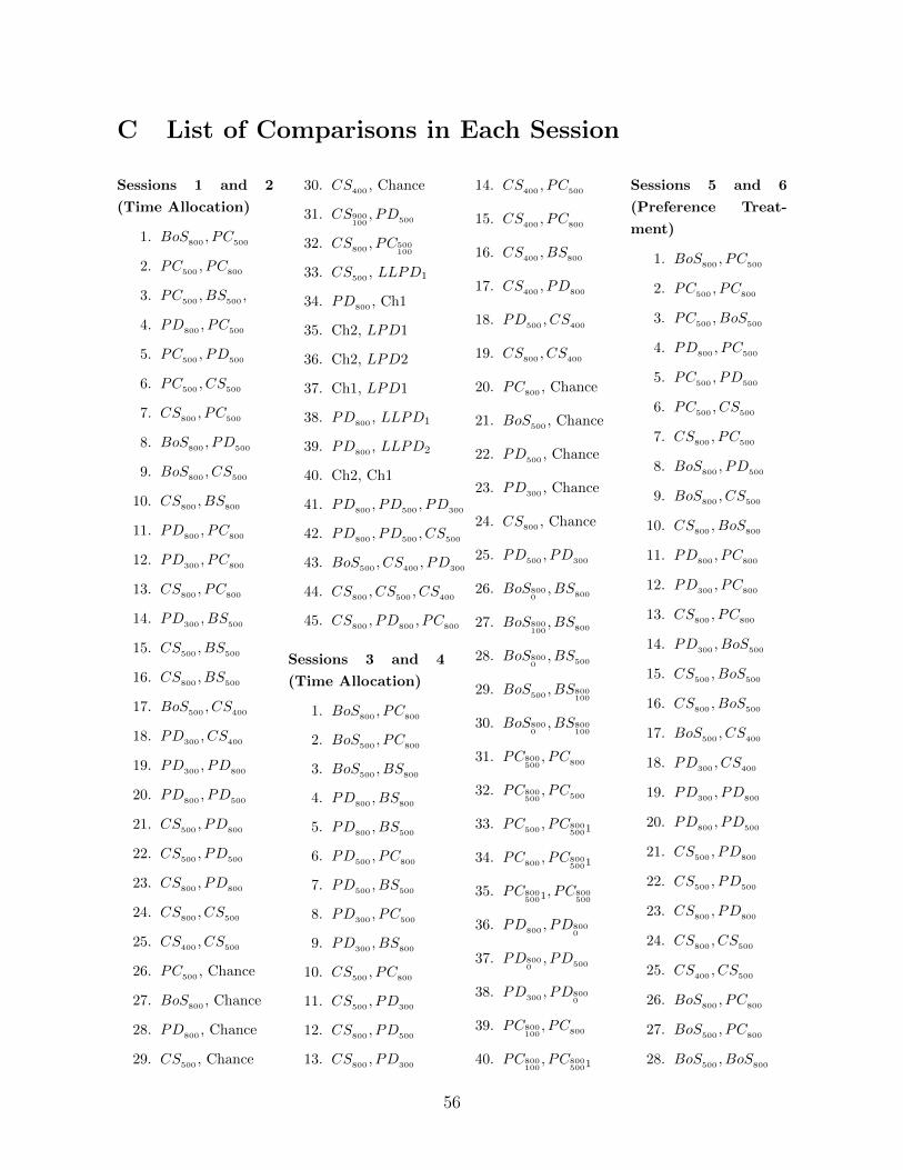
C List of Comparisons in Each Session

Sessions 1 and 2

(Time Allocation)

1. BoS800, PC

500

2. PC500 , PC800

3. PC500, BS

500,

4. PD800 , PC500

5. PC500, PD

500

6. PC500 , CS500

7. CS800, PC

500

8. BoS800, PD

500

9. BoS800, CS

500

10. CS800, BS

800

11. PD800, PC

800

12. PD300, PC

800

13. CS800 , PC800

14. PD300, BS

500

15. CS500 , BS500

16. CS800, BS

500

17. BoS500 , CS400

18. PD300, CS

400

19. PD300 , PD800

20. PD800, PD

500

21. CS500 , PD800

22. CS500, PD

500

23. CS800, PD

800

24. CS800, CS

500

25. CS400, CS

500

26. PC500 , Chance

27. BoS800

, Chance

28. PD800 , Chance

29. CS500

, Chance

30. CS400

, Chance

31. CS900100, PD

500

32. CS800 , PC500100

33. CS500 , LLPD1

34. PD800

, Ch1

35. Ch2, LPD1

36. Ch2, LPD2

37. Ch1, LPD1

38. PD800

, LLPD1

39. PD800

, LLPD2

40. Ch2, Ch1

41. PD800 , PD500 , PD300

42. PD800, PD

500, CS

500

43. BoS500, CS

400, PD

300

44. CS800, CS

500, CS

400

45. CS800 , PD800 , PC800

Sessions 3 and 4

(Time Allocation)

1. BoS800, PC

800

2. BoS500, PC

800

3. BoS500 , BS800

4. PD800, BS

800

5. PD800, BS

500

6. PD500, PC

800

7. PD500 , BS500

8. PD300, PC

500

9. PD300, BS

800

10. CS500, PC

800

11. CS500 , PD300

12. CS800 , PD500

13. CS800, PD

300

14. CS400, PC

500

15. CS400, PC

800

16. CS400, BS

800

17. CS400, PD

800

18. PD500, CS

400

19. CS800, CS

400

20. PC800

, Chance

21. BoS500

, Chance

22. PD500

, Chance

23. PD300

, Chance

24. CS800

, Chance

25. PD500, PD

300

26. BoS8000, BS

800

27. BoS800100, BS

800

28. BoS8000, BS

500

29. BoS500, BS800

100

30. BoS8000, BS800

100

31. PC800500, PC

800

32. PC800500, PC

500

33. PC500, PC800

5001

34. PC800, PC800

5001

35. PC8005001

, PC800500

36. PD800, PD800

0

37. PD8000, PD

500

38. PD300, PD800

0

39. PC800100, PC

800

40. PC800100, PC800

5001

Sessions 5 and 6

(Preference Treat-

ment)

1. BoS800, PC

500

2. PC500, PC

800

3. PC500, BoS

500

4. PD800, PC

500

5. PC500, PD

500

6. PC500, CS

500

7. CS800 , PC500

8. BoS800 , PD500

9. BoS800 , CS500

10. CS800 , BoS800

11. PD800 , PC800

12. PD300, PC

800

13. CS800, PC

800

14. PD300, BoS

500

15. CS500, BoS

500

16. CS800, BoS

500

17. BoS500, CS

400

18. PD300, CS

400

19. PD300, PD

800

20. PD800, PD

500

21. CS500, PD

800

22. CS500, PD

500

23. CS800, PD

800

24. CS800 , CS500

25. CS400 , CS500

26. BoS800 , PC800

27. BoS500 , PC800

28. BoS500 , BoS800

56

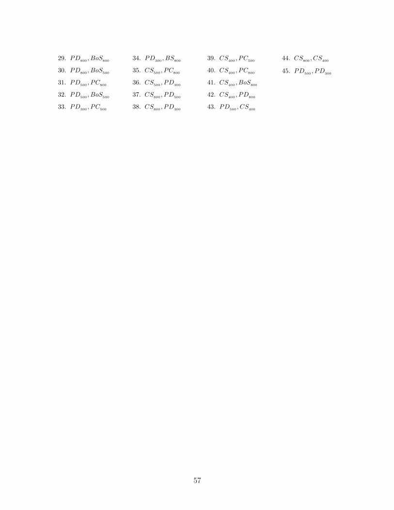
29. PD800, BoS

800

30. PD800 , BoS500

31. PD500 , PC800

32. PD500, BoS

500

33. PD300, PC

500

34. PD300, BS

800

35. CS500, PC

800

36. CS500 , PD300

37. CS800, PD

500

38. CS800, PD

300

39. CS400, PC

500

40. CS400, PC

800

41. CS400 , BoS800

42. CS400, PD

800

43. PD500, CS

400

44. CS800, CS

400

45. PD500 , PD300

57

 

Instructions

This is an experiment in decision making. Funds have been provided to run this experiment and if you make good decisions you may be able to earn a substantial payment. The experiment will be composed of two tasks which you will perform one after the other.

Task 1: Time Allocation

Your task in the experiment is quite simple. In almost all of the 45 rounds in the experiment you will be presented with a description of two decision problems or games, Games 1 and 2. (Actually, in the last 5 rounds you will be presented with some decision problems where there are three games). Each game will describe a situation where you and another person have to choose between two (or perhaps 3) choices which jointly will determine your payoff and the payoff of your opponent. In the beginning of any round the two (or three) problems will appear on your computer screen you will be given 10 (20) seconds to inspect them. Let’s assume that two problems appear. When the 10 seconds are over you will not be asked to play these games by choosing one of the two choices for each of the games, but rather you will be told that at the end of the experiment, if this particular pair of games you are looking at is chosen to be played, you will have X minutes to decide on what choice to make in each of them. Your task now is to decide what fraction of these X minutes to allocate to thinking about Game 1 and what fraction to allocate to thinking about Game 2. To do this you will need to enter a number between 0 and 100 representing the percentage of the X minutes you would like to use in thinking about what choice to make in Game 1 (the remaining time will be used for Game 2).

You will be given 10 seconds to enter this number and remember this will represent the fraction of the X minutes you want to use in thinking about Game 1. If there are two games and you allocate 70 for Game 1, then you will automatically have 30 for Game 2. (If there are ever three games on the screen, you will be asked to enter two numbers each between 0 and 100 whose sum is less than 100 but need not be 100 exactly and you will be given 20 seconds to think about this allocation and 20 seconds to enter your numbers). The first number will be the fraction of X you want to use in thinking about Game 1, the second will be the fraction of the X minutes you want to use in thinking about Game 2, and the remaining will be allocated automatically to thinking about Game 3. For example, if you allocate 30 to Game 1, 45 to Game 2, then you will have 25 left for Game 3, if there are three games. If you do not enter a number within the 10 (or 20) second limit, you will not be paid for that game if at the end this will be one of the games you are asked to play. In other words, be sure to enter your number or numbers within the time given to you.

To enter your time allocation percentages, after the screen presenting the games has closed, you will be presented with a new screen where you can enter your percentage allocations. If you have been shown two games, the screen will appear as follows:

D Time Allocation Treatment

58

In this screen you will need to enter a number between 0 and 100 representing the percentage of your time X that you will want to devote to thinking about Game 1 when it is time for you to play that game if it is one of those chosen.

If you were shown three games your entry screen will appear as follows:

Here you will need to enter two numbers. The first is the percentage of your time X you will devote to thinking about Game 1 before making a choice; the second is the percentage of your time you want to allocate to thinking about Game 2. If the first two number you enter sum up to less than 100, the remaining percentage will be allocated to Game 3.

The amount of time you will have in total, X minutes, to think about the games you will be playing, will not be large but we are not telling you what X is because we want you to report the relative amounts of time you’d like to use of X to think about each problem.

59

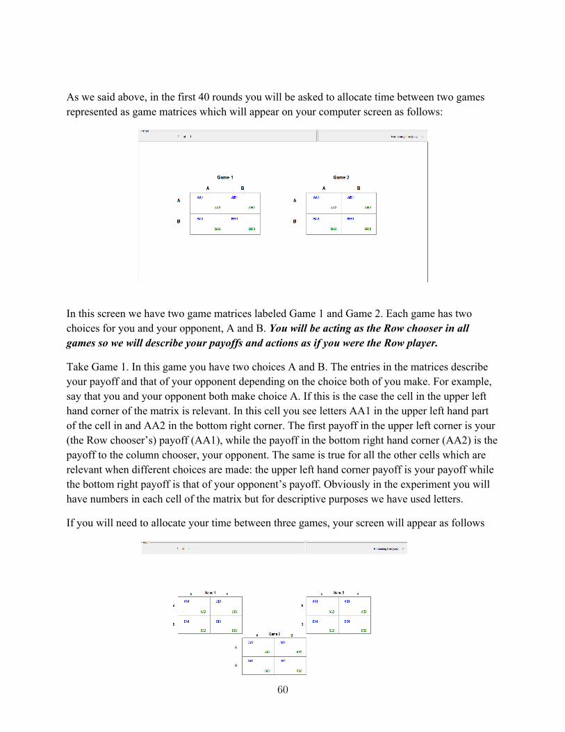
As we said above, in the first 40 rounds you will be asked to allocate time between two games represented as game matrices which will appear on your computer screen as follows:

In this screen we have two game matrices labeled Game 1 and Game 2. Each game has two choices for you and your opponent, A and B. You will be acting as the Row chooser in all games so we will describe your payoffs and actions as if you were the Row player.

Take Game 1. In this game you have two choices A and B. The entries in the matrices describe your payoff and that of your opponent depending on the choice both of you make. For example, say that you and your opponent both make choice A. If this is the case the cell in the upper left hand corner of the matrix is relevant. In this cell you see letters AA1 in the upper left hand part of the cell in and AA2 in the bottom right corner. The first payoff in the upper left corner is your (the Row chooser’s) payoff (AA1), while the payoff in the bottom right hand corner (AA2) is the payoff to the column chooser, your opponent. The same is true for all the other cells which are relevant when different choices are made: the upper left hand corner payoff is your payoff while the bottom right payoff is that of your opponent’s payoff. Obviously in the experiment you will have numbers in each cell of the matrix but for descriptive purposes we have used letters.

If you will need to allocate your time between three games, your screen will appear as follows

60

After you are finished with making your time allocation for a given pair (or triple) of games, you will be given 5 seconds to rest before the next round begins. Please pay attention to your screen at all times since you will want to be sure that you see the screen when a new pair or triple of games appear.

Finally, in very few situations you will have to think about a different type of game which we can call a “Lottery Game”. When you have to choose between two games, one being a lottery game, your screen will appear as follows:

What this says is that you will need to decide between allocating your time between Game 1, which is a type of game you are familiar with, or Game 2 which is our Lottery Game. Game 2 is actually simple. It says that with probability ½ you will play the top game on the screen and with probability ½ you will be playing the bottom game. However, when you play the Lottery Game you must make a choice, A or B, before you know exactly which of those two games you will be playing, that is determined by chance after you make your choice.

For any phase of the experiment, (i.e., when you are allocating time to games or actually choosing) you will see a timer in the upper right hand corner of the screen. This timer will count down how much time you have left for the task you are currently engaged in. For example, on the screen shown above it says you have 6 seconds left before the screen goes blank and you are asked to make a time allocation.

Task 2: Game Playing

When you are finished doing your time-allocation tasks, we will draw two pairs of games and ask you to play these games by making a choice in each game. In other words you will make choices in four games (or possibly more if we choose a triple game for you to play). What we mean by this is that before you entered the lab we randomly chose two of the 45 game-pairs or

61

triples for you to play at the end of the experiment. You will play these games sequentially one at a time starting with Game 1 and you will be given an amount of time to think about your decision equal to the amount of time you allocated to it during the previous time allocation task. So if in any game pair we choose you decided to allocate a percentage y to thinking about Game 1, you will have TimeGame1 = y · X minutes to make a choice for Game 1 before that time elapses and the remaining time, TimeGame2 =X - y·X, left when Game 2 is played. We will have a time count down displayed in the upper right hand corner of your screen so you will know when the end is approaching.

When you enter your choice the following screen will appear.

To enter your choice you simply click on the “Action A” or “Action B” button. Note the counter will appear at the top of the screen which will tell you how much time you have left to enter your choice. (If the game has 3 choices, you will have three action buttons, A, B and C.

You will then play Game 2 and have your remaining time to think about it before making a choice for that game. (If there are three games you will have the corresponding amount of time). If you fail to make a choice before the elapsed time, then your decision will not be recorded for that game and you will receive nothing for that part of the experiment. After you play the first pair of games we will present you with the second pair and have you play them in a similar fashion using the time allocated to them by you in the first phase of the experiment.

62

Payoffs

Your payoff in the experiment will be determined by a three-step process:

1. Before you did this experiment we had a group of other subjects play these games and make their choices with no time constraints on them. In other words, all they did in their experiment was to make choices for these games and could take as much time as they wanted to choose. Call these subjects “Previous Opponents”.

2. To determine your payoff in this experiment, we will take your choice in each pair of games selected and match it against the choice of one Previous Opponent playing the opposite role as you in the game. They will play as column choosers. Remember, the Previous Opponents did not have to allocate time to think about these games as you did but made their choice whenever they wanted to with no time constraint. We did this because we did not want you to think about how much time your opponent in a game might be allocating to a problem and make your allocation choice dependent on that. Your opponent had all the time he or she wanted to make his or her choice.

3. Third, after you have all made choices for both pairs of games, we will split you randomly into two groups of equal numbers called Group 1 and Group 2 and match each subject in Group 1 with a partner in Group 2. We will also choose one of the games you have just played to be the one that will be relevant for your payoffs. Subjects in Group 1 will receive the payoff as determined by their choice as Row chooser and that of their Previous Opponent’s” choice as column chooser. In other words, Group 1 subjects will receive the payoff they determined by playing against a “Previous Opponent”. A subject’s partner in Group 2, however, will receive the payoff of the Previous Opponent. For example, say that subject j in Group 1 chose choice A when playing Game 1 and his Previous Opponent chose choice B. Say that the payoff was Z for subject j and Y for the Previous Opponent. Then, subject j would receive a payoff of Z while subject j’s partner in Group 2 will receive the payoff Y. What this means is if you are in Group 1, although you are playing against an opponent that is not in this experiment, the choices you make will affect the payoff of subjects in your experiment so it is as if you are playing against a subject in this room. Since you do not know which group you will be in, Group 1 or Group 2, it is important when playing the game that you make that choice which you think is best given the game’s description since that may be the payoff you receive. Finally, the payoff in the games you will be playing are denominated in units called Experimental Currency Units (ECU’s). For purposes of payment in each ECU will be converted into UD dollars at the rate of 1 ECU = 0.05 $US.

63

Instructions

This is an experiment in decision making. Funds have been provided to run this experiment and if you make good decisions you may be able to earn a substantial payment. The experiment will be composed of two tasks which you will perform one after the other.

Task 1: Game Preference

There will be 45 rounds in the experiment. In all of the 45 rounds you will be presented with a description of two decision problems or games, Games 1 and 2. Each game will describe a situation where you and another person have to choose between two choices which jointly will determine your payoff and the payoff of your opponent. In the beginning of any round the two problems will appear on your computer screen and you will be given 10 seconds to inspect them. When the 10 seconds are over you will not be asked play these games by choosing one of the two choices for each of the games, but rather to select that game which you would prefer to play with an opponent. At the end of the experiment several of the game-pairs will be chosen for you to play and you will play that game which you said you preferred. So your task now is simply to select one of the two games presented to you in each of the 45 rounds as the game you would prefer to play.

You will be given 10 seconds to enter your preferred game. To do so simply click the button marked Game 1 or Game 2 on the selection screen that appears bellow. If both games look equally attractive to you then click “Indifferent” button and one of the games will be randomly chosen for you.

E Preference Treatment

64

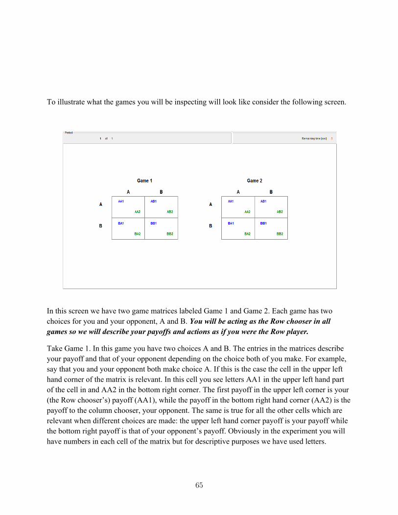
To illustrate what the games you will be inspecting will look like consider the following screen.

In this screen we have two game matrices labeled Game 1 and Game 2. Each game has two choices for you and your opponent, A and B. You will be acting as the Row chooser in all games so we will describe your payoffs and actions as if you were the Row player.

Take Game 1. In this game you have two choices A and B. The entries in the matrices describe your payoff and that of your opponent depending on the choice both of you make. For example, say that you and your opponent both make choice A. If this is the case the cell in the upper left hand corner of the matrix is relevant. In this cell you see letters AA1 in the upper left hand part of the cell in and AA2 in the bottom right corner. The first payoff in the upper left corner is your (the Row chooser’s) payoff (AA1), while the payoff in the bottom right hand corner (AA2) is the payoff to the column chooser, your opponent. The same is true for all the other cells which are relevant when different choices are made: the upper left hand corner payoff is your payoff while the bottom right payoff is that of your opponent’s payoff. Obviously in the experiment you will have numbers in each cell of the matrix but for descriptive purposes we have used letters.

65

After you are finished deciding on which game you prefer, you will be given 10 seconds to rest before the next round begins. Please pay attention to your screen at all times since you will want to be sure that you see the screen when a new pair of games appear.

For any part of Task 1, (i.e., when you are inspecting games or choosing your preferred game), you will see a timer in the upper right hand corner of the screen. This timer will count down how much time you have left for the task you are currently engaged in. For example, on the screen shown above it says you have 5 seconds left before the screen goes blank and you are asked to make a time allocation.

Task 2: Game Playing

When you are finished with Task 1, we will draw two pairs of games and ask you to play the game you said you preferred in Task 1. The other game will not be played so you are best off by choosing that game you truthfully would like to play when given the chance in Task 1. In other words you will make choices in two games. What we mean by this is that before you entered the lab we randomly chose two of the 45 game-pairs for you to play at the end of the experiment. We will then have you play the two games you selected. You will play these games sequentially one at a time.

When you are asked to play a game following screen will appear.

To enter your choice you simply click on the “Action A” or “Action B” button.

66

After you play the first game we will present you with the second game and have you play it in a similar fashion. There is no time limit on how long you can take to make a choice in these games.

Payoffs

Your payoff in the experiment will be determined by a three-step process:

1. Before you did this experiment we had a group of other subjects play these games and make their choices. Call these subjects “Previous Opponents”.

2. To determine your payoff in this experiment, we will take your choice in each pair of games selected and match it against the choice of one Previous Opponent playing the opposite role as you in the game. They will play as column choosers. Remember, the Previous Opponents did not have to allocate time to think about these games as you did but made their choice whenever they wanted to with no time constraint. We did this because we did not want you to think about how much time your opponent in a game might be allocating to a problem and make your allocation choice dependent on that. Your opponent had all the time he or she wanted to make his or her choice.

3. Third, after you have all made choices for both pairs of games, we will split you randomly into two groups of equal numbers called Group 1 and Group 2 and match each subject in Group 1 with a partner in Group 2. We will also choose one of the games you have just played to be the one that will be relevant for your payoffs. Subjects in Group 1 will receive the payoff as determined by their choice as Row chooser and that of their Previous Opponent’s” choice as column chooser. In other words, Group 1 subjects will receive the payoff they determined by playing against a “Previous Opponent”. A subject’s partner in Group 2, however, will receive the payoff of the Previous Opponent. For example, say that subject j in Group 1 chose choice A when playing Game 1 and his Previous Opponent chose choice B. Say that the payoff was Z for subject j and Y for the Previous Opponent. Then, subject j would receive a payoff of Z while subject j’s partner in Group 2 will receive the payoff Y. What this means is if you are in Group 1, although you are playing against an opponent that is not in this experiment, the choices you make will affect the payoff of subjects in your experiment so it is as if you are playing against a subject in this room. Since you do not know which group you will be in, Group 1 or Group 2, it is important when playing the game that you make that choice which you think is best given the game’s description since that may be the payoff you receive. Finally, the payoff in the games you will be playing are denominated in units called Experimental Currency Units (ECU’s). For purposes of payment in each ECU will be converted into UD dollars at the rate of 1 ECU = 0.05 $US.

67