Author's personal copy › ~aheimsat › publications › Heimsath... · (Anderson and Humphrey, 1989; Rosenbloom and Anderson, 1994; Dietrich et al., 1995; Heimsath et al., 1997)

Provided for non-commercial research and educational use only.

Not for reproduction, distribution or commercial use.

This chapter was originally published in the book Hydropedology. The copy attachedis provided by Elsevier for the author's benefit and for the benefit of the author's

institution, for non-commercial research, and educational use. This includes withoutlimitation use in instruction at your institution, distribution to specific colleagues,

and providing a copy to your institution's administrator.

All other uses, reproduction and distribution, including without limitation commercial reprints, selling orlicensing copies or access, or posting on open internet sites, your personal or institution’s website orrepository, are prohibited. For exceptions, permission may be sought for such use through Elsevier’s

permissions site at:http://www.elsevier.com/locate/permissionusematerial

From Heimsath, A.M., 2012. Quantifying Processes Governing Soil-Mantled HillslopeEvolution. In: Lin, H. (Ed.), Hydropedology: Synergistic Integration of Soil Science and

Hydrology. Academic Press, Elsevier B.V., pp. 205–242.ISBN: 9780123869418

Copyright © 2012 Elsevier B.V. All rights reserved.Academic Press

Author's personal copy

http://www.elsevier.com/locate/permissionusematerial

Chapter 7

Quantifying ProcessesGoverning Soil-MantledHillslope Evolution

Arjun M. Heimsath1

ABSTRACTThis chapter presents an overview of how field-based methods quantify the processesshaping upland, soil-mantled landscapes. These methods have been applied acrossdiverse field areas, ranging from the tropical sandstones of northern Australia to thealpine granites of the Sierra Nevada in California. In all cases, the landscapes examinedthrough such work are relatively gently sloping with a generally continuous soil mantle.Soil on such upland landscapes is distinctly defined to be the physically mobile layerderived primarily from the underlying parent material with organic content from nativeflora and fauna. These upland soils are distinguished from agriculture or lowland soils bythe convex-up, hilly topographies that are the focus of this study. Parent material isgenerally saprolite, i.e. weathered bedrock that retains relict rock structure and isphysically immobile. Processes shaping such landscapes include the physical andchemical processes that weather the parent material, and the processes moving the soildownslope. These processes are quantified using several different field-based methods.In situ produced cosmogenic nuclides (10Be and 26Al) are measured in the parentmaterial directly beneath the mobile soil mantle and define the relationship between soilproduction rates and the overlying soil thickness. The same cosmogenic nuclides aremeasured in detrital sediments sampled from local channels to quantify basin-averagederosion rates. Mobile and trace elements are measured in both the parent material andthe soils to define chemical weathering rates and processes. Short-lived, fallout-derivedisotopes (210Pb, 137Cs, and 7Be) are measured in soil profiles to quantify sediment-transport processes and short-term erosion rates. Parent material strength (competence),or resistance to shear, is measured using a hand-held shear vane as well as a conepenetrometer. The methodology for some results and the connections drawn from thisdiverse toolbox are summarized in this chapter. An important conclusion connectingparent material strength to the physical processes transporting soil and the chemicalprocesses weathering the parent material emerges with the observation that parentmaterial strength increases with overlying soil thickness and, therefore, the weatheredextent of the saprolite. This observation highlights the importance of quantifying

1School of Earth and Space Exploration, Arizona State University, AZ, USA.

Email: [email protected]

Hydropedology, Edited by H. Lin. DOI: 10.1016/B978-0-12-386941-8.00007-1

Copyright � 2012 Elsevier B.V. All rights reserved. 205

Hydropedology, First Edition, 2012, 205–242


hillslope hydrologic processes at the same locations where the measurements describedherein are made. Specifically, by understanding the hydrologic pathways that help drivethe weathering processes of upland soils and saprolites, we will gain considerablygreater insight into how the processes described in this chapter drive landscapeevolution.

1. INTRODUCTION

Quantifying the rates of Earth surface processes across soil-mantled landscapesis critical for many disciplines (Anderson, 1994; Bierman, 2004; Dietrichet al., 2003; Dietrich and Perron, 2006). Balances between soil production andtransport determine whether soil exists on any given landscape, as well as howthick it might be. Soil presence and thickness, in turn, help support much of thelife that we humans are familiar with, play important roles in the hydrologiccycle, and are coupled with processes that impact the atmosphere. Similarly,sustainability of the Earth’s soil resource under growing human populationpressures also depends on the balance between soil production and erosion:agriculture depends on soil. Fully quantifying the conditions that will lead toa depletion of the soil resource is as important, in my opinion, as quantifying thedegradation of our drinking water. As such, the near-surface environment thatincludes soil and its parent material is known as the Critical Zone (CZ) and is thefocus of exciting new research initiatives, including the NSF-supported CriticalZone Observatory program (Amundson et al., 2007; Anderson et al., 2004;Anderson et al., 2007; Brantley et al., 2007). Over the last ten years, significantprogress in the field (e.g. Anderson and Dietrich, 2001; Burkins et al., 1999;White et al., 1996; Yoo et al., 2007), lab (e.g. White and Brantley, 2003), andwith modeling (e.g. Minasny and McBratney, 2001; Mudd and Furbish, 2006)has enabled a new level in understanding how forces of sediment production andtransport shape landscapes and help determine the viability of the Earth’s soilresource (Montgomery, 2007). Despite this progress, there are significant gaps inour understanding of this interface between humans, the atmosphere, biosphere,and lithosphere. One of the most significant gaps is quantifying what controls soilthickness (Anderson et al., 2007; Brantley et al., 2007), while another is thecontinued quantification of the sediment-transport relationships (cf GeomorphicTransport Laws, Dietrich et al., 2003; Heimsath et al., 2005). The focus of thischapter is on soil-mantled, upland landscapes to provide an overview of how wequantify the rates and processes active in shaping such landscapes. This chapteris not a comprehensive review of the field, but does serve well to review some ofthe key methods and results applied on these landscapes.

Hilly and mountainous landscapes around the world are mantled withsoil. In regions where external sources of sediment (e.g. eolian and glacialdeposition) are absent or negligible, the soil mantle is typically producedfrom the underlying bedrock. Gilbert (1877) first suggested that the rate of

206 PART | I Overviews and Fundamentals



soil production from the underlying bedrock is a function of the depth of thesoil mantle. We term this rate law the soil production function (Heimsathet al., 1997) – defined as the relationship between the rate of bedrockconversion to soil and the overlying soil thickness. This soil depth that setsthe rate of soil production is a result of the balance between the soilproduction and erosion. If local soil depth is constant over time, the soilproduction rate equals the erosion rate, which equals the lowering rate of theland surface. Quantifying the soil production function therefore furthersour understanding of the evolution rates of soil-mantled landscapes(Anderson and Humphrey, 1989; Rosenbloom and Anderson, 1994; Dietrichet al., 1995; Heimsath et al., 1997). Heimsath et al. (1997, 1999, 2000)reported spatial variation of erosion rates, suggesting that the landscapeswere out of the state of dynamic equilibrium, as first conceptualized byGilbert (1877, 1909) and then Hack (1960). Such a condition, where thelandscape morphology is time-independent, was an important assumption forlandscape evolution models. Showing that upland landscapes are actuallyevolving with time helped spur a new level of understanding for howlandscapes change under climatic and tectonic forcing.

On actively eroding hilly landscapes, characterized by ridge and valleytopography (Fig. 1), the colluvial soil mantle is typically thin and is produced andtransported by mechanical processes. Tree throw, animal burrowing, and similarprocesses, such as freeze–thaw and shrink–swell cycles, convert in-placebedrock to a mobile, often rocky, soil layer that is then transported downslope bythe same actions (Lutz and Griswold, 1939; Lutz, 1940; Lutz, 1960; Hole, 1981;Mitchell, 1988; Matsuoka, 1990; Schaetzl and Follmer, 1990; Norman et al.,1995; Paton et al., 1995). On steep slopes, shallow landsliding also transports

FIGURE 1 Photograph of a typical hilly, soil-mantled landscape that is the focus of work

described in this chapter. Point Reyes, California. (Photo by the author) (Color version online)

207Chapter | 7 Quantifying Processes Governing Soil-Mantled Hillslope



material downslope, and may also play a role in producing soil. While suchprocesses are aided directly, and even accelerated, by chemical weathering of thebedrock, they are able to produce soil from bedrock irrespective of its weatheredstate. Early quantification of the soil production function focused on low-gradient topography developed on relatively homogeneous bedrock, wheresimple rate laws can characterize the geomorphic processes (Heimsath et al.,1997, 1999, 2000, 2009). Methods applied in those studies were also applied tosteep, landslide-dominated landscapes to extend our understanding of theconnections between soil production, erosion, and landscape evolution (Heim-sath et al., 2001a; Heimsath et al., 2012).

In this chapter, I review the conceptual framework used to quantify soilproduction and hillslope weathering rates, and explore the field measurementsthat we make to connect processes governing hillslope hydrology with soilproduction and transport. Specifically, I will review the mass-balance approachused to model landscape evolution and identify the key field-based parametersthat we quantify with direct measurements. These measurements include (1)cosmogenic nuclides (10Be and 26Al) to quantify soil production andcatchment-averaged erosion rates, (2) major and trace element analyses toquantify the weathered state and weathering rate of the parent material and soil,(3) short-lived isotopes (137Cs and 210Pb) and optically stimulated lumines-cence (OSL) to quantify soil transport processes, and (4) cone penetrometer andshear vane measurements to quantify the competence of the parent materialunderlying the actively eroding soil mantle (i.e. its resistance to physicaldisruption). This chapter is deliberately focused on expanding upon themethods that we use to examine hilly and mountainous landscapes that arecontinuously mantled with soil, which is actively produced from the underlyingparent material. Instead of focusing on any specific field site, which our variouspapers do, I will present representative results in a more general way to enablethe discussion that will conclude this chapter. To help provide context for theseresults drawn from different landscapes and studies, I provide a brief overviewof how they are all related following the summary of the conceptual frameworkand methods.

2. CONCEPTUAL FRAMEWORK AND METHODS

2.1. Soil Production and Chemical Weathering

Consider a depth profile at a hillcrest, extending from the soil surface tounweathered bedrock (Fig. 2). The layer of physically and/or chemicallyaltered material (saprolite and soil) atop crystalline bedrock can be millimetersto tens of meters thick depending on the landscape in question and the externaldriving forces eroding the landscape. A number of definitions are foundthroughout the literature for these terms; here, ‘soil’ is the physically mobilematerial that is produced by the mechanical disruption of the underlying




bedrock (Fig. 2b), or saprolite (Fig. 2c). Saprolite is the nonmobile, weatheredmantle produced by chemical alteration of the bedrock that lies beneath. At theupper boundary, saprolite is incorporated into the mobile soil column throughphysical disruption by soil production mechanisms such as tree throw, macro-and microfauna burrowing, and frost cracking. At the lower boundary, saproliteis produced from parent bedrock by chemical dissolution and mineral trans-formation. While mineralogical changes and alteration occur throughout thesaprolite column, much of the chemical mass loss can occur as a discreteweathering front near the bedrock boundary (Frazier and Graham, 2000; Busset al., 2004; Fletcher et al., 2006; Lebedeva et al., 2007; Buss et al., 2008).We focus specifically on the mass loss due to chemical processes (here termedchemical weathering) and physical processes (here termed erosion) on soil-mantled hillslopes. By these definitions, weathering within saprolite is purelychemical, while soils evolve by both chemical transformations and physicaldisruption and erosion.

Using basic mass conservation principals, any change in soil mass,expressed as the product of soil density (rsoil) and change in soil thickness (h),reflects the mass rates (determined with the appropriate bulk densitymeasurements times the rate) of soil production (Psoil), erosion (E), andweathering (Wsoil), such that

rsoilvh

vt¼ Psoil � E �Wsoil: (1)

Soil-Rock System Soil-Saprolite-Rock System(a) (b)

E

E

Dtotal

Dtotal

wsoil

wsoil

wsaprolitePsaprolitePsoil

Soil h

Psoil

Soil h

BedrockBedrock

Saprolite

(c)

FIGURE 2 Conceptual cross section of soil–saprolite–bedrock showing fluxes and symbols.

Soils may be mechanically produced from bedrock (a) or weathered saprolite (b). Based on

conservation of mass Eqns (1) and (2) in text, if soils have a steady-state thickness, then soil

production (Psoil) is balanced by weathering (Wsoil) and erosion (E). If saprolite thickness attains

a similar steady state, then saprolite production (Psap) is balanced by mass loss from the saprolite

profile by weathering (Wsap) and the mechanical conversion to soil (Psoil). Note that total denu-

dation rate (Dtotal) is calculated from the sum of losses, and reflects only erosion and weathering in

soil in Fig. 1a, but accounts for the additional losses due to saprolite weathering in Fig. 1b. (c)

Photograph of a typical soil-weathered bedrock boundary with gopher burrow shown penetrating

the light-colored saprolite. (From Dixon et al., 2009a)




If soil thickness (h) is constant over time

�vh

vt¼ 0

�, then the rate of soil mass

loss equals the rate of soil production:

Psoil ¼ E þWsoil: (2)

The sum of all rates of mass loss can be termed the total denudation rate (DT),and these losses occur by physical erosion of soil and chemical weathering inboth the soil (Wsoil) and the saprolite (Wsap), such that (Fig. 2c)

DT ¼ E þWtotal ¼ E þWsoil þWsap: (3)

Recalling mass conservation for steady-state soil thickness Eqn (2), and Eqn (3)can be written as

DT ¼ Psoil þWsap: (4)

It is important to note from Eqn (4) that the soil production rate (Psoil) issmaller than the total denudation rate (DT) in a landscape that experienceschemical weathering in the saprolite. Furthermore, Psoil, which can representa rate of mass flux, can be converted to a landscape lowering rate in units oflength per time by dividing by saprolite density if the analyses are done in massloss per time. DT cannot as easily be converted into a lowering rate because ofits associated saprolite weathering term in Eqn (4); saprolite weathering isobserved to be isovolumetric for the studies examined through this conceptualframework, and mass is lost from the saprolite without a corresponding changein volume.

Rates of chemical weathering in catchments have commonly beenquantified using stream solute data. These measurements provide a valuablequantification of instantaneous weathering, but provide limited insight intolandscape evolution due to their short measurement timescales (1–10 y) andbecause they integrate mass losses from all points within the catchment, thustreating a watershed as a black box. Riebe et al. (2003a) developed a methodto calculate chemical weathering rates in actively eroding terrains bycoupling a mass-balance approach using immobile elements (Brimhall et al.,1992; Brimhall and Dietrich, 1987) to rates of landscape lowering derivedfrom cosmogenic radionuclides (CRNs). CRNs such as 10Be and 26Alprovided a tool to measure surface rates of denudation over longer timescales(103–105 y) than solute measurements (1–10 y). These longer timescales,though still only a fraction of the evolutionary period of some landscapes, aremore relevant to studies examining the influence of external forcing (climateand tectonics) on landscape change.

CRN concentrations in a sample of rock, saprolite, or soil record therate of surface denudation processes that removed overlying mass, and




therefore the rate at which the sample approaches the land surface(Lal, 1991):

DCRN ¼ P0L

N: (5)

Here, the CRN-derived surface denudation rate (DCRN; g cm�2 y�1) isa function of the measured CRN concentration in quartz (atoms g�1), the CRNproduction rate at the surface (P0: atoms g�1 y�1), which decreases expo-nentially with depth, and the CRN attenuation length (L; g cm�2). A completeversion of Eqn (5), used to calculate rates in this chapter, is presented anddiscussed thoroughly by Balco et al. (2008); however, the simplified versionshown by Eqn (5) is sufficient for the purposes of our discussion. For 10Be,the most widely used CRN for determining landscape denudation rates,the penetration depths of cosmic rays, assuming a mean attenuation of160 cm2 kg�1, are ~140 cm through soil and ~60 cm through rock (Balcoet al., 2008). Nuclide concentrations, therefore, record near-surface massremoval within the top few meters of the Earth’s surface, and therefore willreflect both chemical and physical losses within soil (typically less than 2 mthick); however, mass losses due to chemical weathering at the bedrock–saprolite boundary are likely to occur at deeper depths than recorded byCRNs. These losses remain unknown and highlight an outstanding researcharea for future work. A sample of soil, saprolite, or rock will, therefore, havea 10Be concentration that reflects the rate at which overlying soil wasremoved. Assuming local steady-state soil thickness (Eqn (2)), this rate isequivalent to the soil production rate (Heimsath et al., 1997, 1999; Heimsath,2006):

DCRN ¼ Psoil: (6)

Here, we caution that the generic term denudation (DT) should not beused to specifically denote CRN-derived rates of landscape lowering. CRN-derived rates do not capture the result of deep saprolite weathering, and thusonly record a portion of total denudation on deeply weathered landscapes. Asa consequence, we distinguish between soil production rates (Psoil) that equalCRN-derived surface denudation rates (DCRN) and total denudation rates (DT)that reflect combined rates of mass loss in soil and saprolite due to physicaland chemical processes. To fully quantify the potential mass loss from deepsaprolite chemical weathering, we expand upon previously developedmethods for determining soil production, erosion, and chemical weatheringrates.

The enrichment of an immobile element in a weathered product relativeto the parent material can be used to calculate the fraction of mass thatwas lost to chemical weathering (Brimhall et al., 1992; Brimhall and




Dietrich, 1987). Riebe et al. (2001b) termed this relationship the chemicaldepletion fraction (CDF):

CDF ¼�1� ½I�p

½I�w

�; (7)

where the subscripts ‘p’ and ‘w’ refer to concentrations of the immobileelement (I ) in the parent material and weathered material, respectively.For accurate calculation of the CDF, several important conditions must bemet: homogeneous parent material, chemical immobility of the referenceelement, and minimal chemical weathering during lateral soil transport,which is also an area of active research. Additionally, we must assume noinputs of the immobile element by volcanic ash or continental dust, althoughthis highlights the need for further studies to fully constrain such potentialinputs.

Equation (7) can be used to represent the chemical depletion fraction due tosoil weathering, saprolite weathering, or total weathering processes. We termthese respective depletion fractions the CDFsoil, CDFsap, and CDFtotal, and eachis written as Eqn (7), replacing the generic immobile element ‘I’, with theelement zirconium, which is immobile in most weathering environments(e.g. Green et al., 2006).

Following Riebe et al. (2003a), the total chemical weathering rate is theproduct of the total denudation rate and the total CDF:

Wtotal ¼ DT ��1� ½Zr�rock

½Zr�soil

�¼ DT � CDFtotal: (8)

Here, the CDFtotal represents the fraction of total denudation (DT) that occurs byall chemical losses (in both the saprolite and the soil). Assuming steady-statesoil and saprolite thickness, the saprolite weathering rate can be similarlywritten (Dixon et al., 2009a). The soil weathering rate is then the calculateddifference between Wtotal and Wsap.

Calculations of chemical weathering and erosion rates require themeasurement of CRN-derived soil production rates. Taking this into account,we rearrange the equations for erosion and weathering in terms of CRN-derivedPsoil (Eqn (5)). The weathering rate of soil (Wsoil) is calculated as the product ofPsoil and the CDFsoil:

Wsoil ¼ DT ��1� ½Zr�saprolite

½Zr�soil

�¼ Psoil � CDFsoil: (9)

Here, the CDFsoil represents the fraction of original saprolite mass lost due tochemical weathering. The erosion rate (E) can then be calculated as thedifference between Psoil and Wsoil (following Eqn (2)).

Lastly, the rate of saprolite weathering (Wsap) is calculated by returning tobasic principles regarding conservation of mass for immobile elements. For




a chemically immobile element such as Zr, the conservation of mass equationcan be written as

Psap � ½Zr�rock ¼ Psoil � ½Zr�saprolite ¼ E � ½Zr�soil: (10)

Here, Psap (Fig. 2b) represents the rate conversion of rock to saprolite, and ismathematically equivalent to the total denudation rate (DT) assuming a steady-state regolith thickness. Solving for total denudation yields

DT ¼ Psap ¼ Psoil

�½Zr�saprolite½Zr�rock

�: (11)

Substituting Eqn (11) into a form of Eqn (8) for saprolite then gives us theequation for the saprolite weathering rate (Wsap):

Wsap ¼ Psoil ��½Zr�saprolite

½Zr�rock� 1

�: (12)

Summing calculated weathering and erosion rates from these equations allowsone to calculate the total denudation rates (Eqn (3)) (Dixon et al., 2009a). Theseequations differ from those of Riebe et al. (2003a) by the definition that CRN-derived rates reflect only soil production rates, and not total denudation rates inregions mantled by saprolite.

2.2. Soil Transport

The conceptual framework used for our studies is based on the equation of massconservation for physically mobile soil overlying its parent material (Carson andKirkby, 1972; Dietrich et al., 1995). Typically, the boundary between soil and theunderlying weathered (or fresh) bedrock is abrupt and can be defined withina few centimeters. Soil is produced and transported bymechanical processes, andsoil production rates decline exponentially with depth (Heimsath et al., 1997,2000). The transition from soil-mantled to bedrock-dominated landscapes occurswhen transport rates are greater than production rates (Anderson and Humphrey,1989) and two transport functions are typically used to model landscapeevolution (Braun et al., 2001; Dietrich et al., 2003). The slope-dependenttransport law has its basis in the characteristic form of convex, soil-mantledlandscapes assumed to be in equilibrium, and has some field support(e.g. McKean et al., 1993; Roering et al., 2002). A nonlinear, slope-dependenttransport law also has its roots in morphometric observations, and has recentsupport with the veracity of assuming landscape equilibrium (Roeringet al., 1999), experimental constraints (Roering et al., 2001), or for landscapeswhere postfire ravel processes are thought to dominate (Gabet et al., 2003;Roering and Gerber, 2005; Lamb et al., 2011).




Mechanistically, soil transport should depend on soil thickness as well asslope, as suggested by quantification of freeze–thaw (e.g. Anderson, 2002;Matsuoka and Moriwaki, 1992), shrink–swell (e.g. Fleming and Johnson,1975), viscous or plastic flow (e.g. Ahnert, 1976), and bioturbation processes(Gabet, 2000). In each case, disturbance processes set the mobile soilthickness and modulate soil transport by setting the magnitude of slope-normal displacement, while slope sets the downslope component of thegravitational driving force. Depth-dependent flux is also suggested by thevelocity profiles from segmented rod studies and modeling (Young, 1960;Young, 1963). For flux to be proportional to the depth–slope product is anidea that has never been tested despite being suggested almost 40 years ago(Ahnert, 1967).

Recently, Furbish (2003) suggested that for transport due to dilationaleffects of biotic activity, the vertically averaged volumetric flux density (i.e.vertically averaged velocity), qs (L t�1), is proportional to land surfacegradient, S. The depth-integrated flux per unit contour distance is then theproduct of soil thickness, H, and this flux density

Hqs ¼ �KhHS; (13)

where Kh (L t�1) is a transport coefficient, assumed to be constant. We testedthis transport relation using estimates of local depth-integrated flux, Hqs,obtained by integrating the soil production rate between flow lines at threedistinct field sites (Heimsath et al., 2005), and found support for the depth-dependent transport relationship (Furbish et al., 2009). Importantly, our workquantifying the soil production function using both CRNs and the morpho-metric test of plotting topographic curvature against soil thickness also supportsthe slope-dependent transport relationship (Heimsath et al., 1997, 1999, 2000,2006). Clearly, more direct quantification of the soil transport processes isneeded and some of our studies are pursuing this actively.

Long-standing efforts to determine average erosion rates across agriculturallandscapes involve the construction of small-scale runoff plots (Roels, 1985),monitoring of suspended sediment concentrations in streams draining thelandscapes (Steegen et al., 2001), and, with recent analytical breakthroughs,through the use of sediment tracers (Matisoff et al., 2001) or short-lived isotopes(Wilson et al., 2003; Matisoff et al., 2002a,b). Collection and analyses of soilfrom runoff plots or suspended sediment analyses remain problematic primarilybecause of the difficulties with ensuring a closed system, while injection oftracers onto agricultural lands immediately imparts a short-term measurementbias. Attempts to quantify sediment-transport processes include segmented rodstudies (Young, 1960), tephra deposit mapping (Roering et al., 2002), detailedmeasurement of bioturbation (Black and Montgomery, 1991; Gabet, 2000),optically stimulated luminescence dating of individual quartz grains (Heimsathet al., 2002), and short-lived isotope measurements (Wallbrink and Murray,1996; Walling and He, 1999; Kaste et al., 2007; Dixon et al., 2009a). Despite the




extensive effort across disciplines, quantifying sediment-transport processes andrates remains elusive (Dietrich et al., 2003).

During the middle of the twentieth century, the detonation of nuclear weaponsin the atmosphere injected a host of artificial radionuclides into the environmentwith half-lives ranging from days to decades. While atmospheric weapons weretested in various countries from the 1940s until the late 1970s, the vast majority offallout in the central United States was deposited between 1955 and 1967(Cambray et al., 1989; Simon et al., 2004). These fallout radionuclides offera unique tool for determining time-integrated erosion rates on a landscape withonly one or a few visits to the site (Brown et al., 1981a; Brown et al., 1981b;Zhang et al., 1994;Quine et al., 1997;Walling et al., 1999;Walling et al., 2002;Heand Walling, 2003; Porto et al., 2003; Fornes et al., 2005). Fallout radionuclidesare used extensively in erosion and sediment-transport studies on both agriculturaland forested landscapes. Atmospherically delivered 210Pb (T1/2¼ 22.3 y, 210Pbex,“in excess” of that supported bydirect decay of 222Rn in soil), cosmogenic 7Be (T1/

2¼ 53d), andweapons-derived 137Cs (T1/2¼ 30.1 y) and 241Am(T1/2¼ 432y) canbe used alone or simultaneously to quantify and trace erosional processes(Wallbrink andMurray, 1996;Walling et al., 1999;Whiting et al., 2001), date andsource sediments (Appleby and Oldfield, 1992), and determine sediment transittimes (Bonniwell et al., 1999). Fallout radionuclides are useful geomorphic toolsbecause of their unique atmospheric source term, but the technique relies on theassumption that the radionuclides are geochemically immobile and thus effectiveparticle tracers.

Relative rates of soil mixing can be evaluated through measurements offallout nuclide activities in soil profiles (Dorr, 1995; Tyler et al., 2001). Becausethese atoms are deposited at the soil surface, mixing processes can increase thedispersion of nuclides with depth and the overall downward transport rate. Forexample, on agricultural landscapes, where tilling homogenizes the soil to thedepth of the plow layer, a unique, well-mixed 137Cs profile captures the process(Walling et al., 1999). Field evidence suggests that some soils are homogenizednaturally by burrowing organisms (Heimsath et al. 2002; Black and Mont-gomery, 1991), which would mix fallout isotopes down to a depth governed bythe flora and fauna at the site. However, in some undisturbed forest soils wherebioturbation is less obvious, the transport mechanisms can be more elusive anddifficult to quantify. By measuring the vertical distribution of fallout radionu-clides in soils and calculating diffusion coefficients, we can quantify sediment-transport mechanisms and mixing rates that are operating on the short butimportant timescale of 10–100 years.

The techniques of relating fallout radionuclide profiles and inventories toabsolute and relative erosion rates rely on finding a “noneroding” referencelocation to compare to eroding or aggrading sites (Lowrance et al., 1988).Nearly all erosion studies by other research groups compare soils sampledat cultivated sites with those sampled from an undisturbed field or forest.We examined soil mixing and transport processes across our soil-mantled




hillslopes using fallout radionuclides and by observations of biologicalactivity in the field. We measured 210Pbexcess (here, shortened to 210Pb) and137Cs nuclide activities with depth and calculated total inventories, to gaininsight into mixing (e.g. Kaste et al., 2007; Dixon et al., 2009a) and soilerosion mechanisms (e.g. Kaste et al., 2006; O’Farrell et al., 2007). Thenuclide profile depth was defined as the soil depth at which greater than 95%of the cumulative nuclide activity, or inventory, was obtained. We usednuclide profiles to determine the degree of physical mixing, and calculateda mixing coefficient by the best-fit exponential curve to an advection–diffu-sion equation (Kaste et al., 2007).

Steady-state profiles of 210Pb provide insight into mixing and soil transportover short timescales (102–103 years). The depth distribution of 210Pb in soilscan be described by the steady-state solution to the advection–diffusionequation (e.g. He and Walling, 1996; Kaste et al., 2007):

AðzÞ ¼ A0 exp

"v� ffiffiffiffiffiffiffiffiffiffiffiffiffiffiffiffiffiffiffi

v2 þ 4lDp

2DðzÞ

#; (14)

where ‘A(z)’ is the nuclide activity at a specific depth (in Bq cm�3), ‘A0’ is theactivity at the surface, ‘v’ is the downward advection velocity due to leaching(cm y�1), ‘l’ is radioactive decay (y�1), and ‘D’ is a diffusion-like mixingcoefficient (cm2 y�1). Advection rates have previously been measured using thedepth of concentration of weapons-derived 137Cs, which was delivered to soilsas a thermonuclear bomb product between 1950 and 1970, peaking in 1964(e.g. Kaste et al., 2007). We were sometimes unable to determine clearsubsurface peaks in 137Cs activity profiles that correspond to this delivery.Instead, in such cases, we calculated diffusion-like mixing coefficients byassuming that advection plays a minimal role in subsurface nuclide redistri-bution. We then modeled a best-fit diffusion equation to each profile byminimizing the sum of residuals. Importantly, the timescale of such quantifi-cation is only appropriate for recently (~10 to <100 years) active processes.

2.3. Parent Material Strength

The depth dependency of soil production rates followed Gilbert’s earlyreasoning that rock disintegration was fastest under thin soils and slowed wherebedrock emerged at the surface or was deeply mantled with soil. Gilbertbelieved that on a steady-state landscape, where erosion is equaled by soilproduction, highest erosion rates would be under thin soils and lowest rateswould be at the extremes because (i) exposed bedrock would limit transport tothe slow rate of exposed and coherent rock and (ii) thick soil cover woulddevelop for low transport rates. While this conceptual framework persisted(Carson and Kirkby, 1972) and was explored extensively (Ahnert, 1967;Anderson and Humphrey, 1989; Cox, 1980; Dietrich et al., 1995; Heimsath




et al., 1997; Minasny and McBratney, 1999), the underlying mechanismsgoverning it remain fundamentally untested. The sharp boundary betweensaprolite and soil as well as the biogenic disruption by gopher burrowing, ants,earthworms, and burrowing wombats (Australia) are widely observed, high-lighting the role of parent material weatherability in setting the upper bound forsoil production, as well as biogenic role in downslope transport. Additionally,quantifying parent material strength at locations where soil production andtransport rates as well as chemical weathering rates are known helps make theconnection between hillslope hydrology and the geomorphic processes drivinglandscape evolution.

Specifically, the parent material resistance to the physical processes thatconvert it to transportable sediment is likely to reflect the intersection of severalaspects of forces driving landscape evolution. First, tectonic forces set the baselevel that upland landscape evolution is thought to be responding to. Second,climatic forces set both the biota (i.e. flora and fauna) providing the physicalforces of hillslope weathering, and the chemical weathering parameters thatbreak down minerals and remove mass in solution. Third, the combination ofphysical and chemical weathering processes is likely to determine just howweathered (and therefore resistant to shear) the parent material becomes. Forexample, active bioturbation that mixes a soil thoroughly also helps conveywater and organic acids to the soil-parent material boundary. Conversely,a landscape lacking bioturbation and experiencing active overland flowprocesses is likely to have a smaller degree of contact between meteoric watersand the parent material. Understanding hillslope hydrologic pathways are,therefore, critically important for coupling the physical and chemical processesthat we have focused on thus far. Quantifying all of the different processes andparameters that factor into how hillslopes are evolving thus enables us to betterpredict how landscapes are likely to change with the changing driving forces ofclimate, tectonics, and anthropogenic.

We apply independent, field-based measurements to quantify the strength(i.e. resistance to shear) of the parent material underlying the mobile soil layer.Quantifying strength can be done in a number of ways. Selby (1980, 1985)suggests a semiquantitative classification of rock mass strength for crystallinebedrock. Although this method is comprehensive and appropriate for rockyslopes, it is difficult to compare with soil-mantled slopes where we are inter-ested in the saprolite resistance to physical disruption. Several studies haveexplored the physical characteristics of granitic and metamorphic rocks andsaprolites, but have mostly focused on groundwater saturation effects and slopestabilities (e.g. Jiao et al., 2005; Johnson-Maynard et al., 1994; Jones andGraham, 1993; Kew and Gilkes, 2006; Schoeneberger et al., 1995). It isimportant to note that the complexities inherent in quantifying the strength ofcompetent rocky slopes are lessened by the fact that we are interested inquantifying the resistance of a relatively continuous layer of weathered materialthat is overlain by a relatively smooth surface mantle of soil.




We use two instruments to assess saprolite strength: a dynamic-conepenetrometer and a shear vane tester (Herrick and Jones (2002) andGEONOR). We also experimented with Schmidt hammers (see recentreview article and results in Viles et al. (2011)), but their dependence ongrain boundaries and limited applicability to competent bedrock meant thatwe could not use them for saprolitic parent material (i.e. anything expe-riencing even the slightest degree of weathering). The penetrometermeasures the compressibility of a material in units of strikes per depth,which can be converted to kPa when calibrated with the shear vane tester.The shear vane tester measures the shear strength in kilopascals (kPa). Weused a Geonor H-60 handheld vane tester (GEONOR) with an instrumentrange from 0 to 260 kPa. The standard procedure is to place the end of thevane normal to the surface and insert it about 5 cm below the surface tominimize any edge effects, then turn the handle clockwise at a constant rateuntil the lower and upper portions of the instrument move in unison,indicating that the maximum shear strength has been obtained. Otherstudies have explored the correlation between these two instruments atdifferent sites (Bachmann et al., 2006; Zimbone et al., 1996). The shearstrength of a soil is directly related to the normal stress applied (McKyes,1989); therefore, an instrument that applies a force normal to the surfacecan be used to estimate a relative shear strength. Several field seasons ofexperimenting with these instruments led us to a procedure that appears toyield reproducible and reliable results (Byersdorfer, 2006; Johnson, 2008).

3. FIELD SITE SUMMARY

To tie together the methods outlined above, I draw upon studies acrossa few selected field areas examined by my research group. It is beyond thescope of this chapter to go into all the details, or expand upon all of thespecific assumptions and caveats for each of these study areas, but there arekey aspects of the sites that I summarize here to help navigate theconnections between the conceptual framework and the representativeresults. Recall that a key assumption used to develop the conceptualframework is the assumption that soil thickness does not change with timelocally. This does not mean that soil thickness is uniform across thelandscape, but it does mean that our initial site selection was motivatedby convincing ourselves that local soil thickness remains constant(excluding the stochastic perturbations associated with bioturbation that arerelatively quickly “healed”). A similarly important criterion for site selec-tion was that the processes we observe today reflect the processes drivinglandscape evolution over the timescales captured by our methodologies(tens to tens of thousands of years). Three field areas were, therefore, theinitial focus of our studies: Tennessee Valley (TV), California, Point Reyes(PR), California, and Nunnock River (NR), southeastern Australia. Each of




these field sites has smoothly convex-up soil-mantled ridges separated byunchanneled, “zero-order” swales and also had independent studies, sug-gesting that the impact of the Pleistocene–Holocene transition on localbiota was not severe. Two of these field sites (PR and NR) have graniticparent material, while TV has metasedimentary rock. The relative ease ofworking on granitic parent material drove further studies to focus ongranitic landscapes, where possible.

Following the honing of methodology across these field sites, weexpanded our studies to include an examination of the role of climaticforcing. For that work we used a climate transect in the southern SierraNevada Mountains (Dixon et al., 2009a,b) and I summarize some of thatwork here by focusing on the climate end members of the alpine region ofWhitebark (WB) and the oak-grassland region at Blasingame (BG).We worked in parallel to examine the role of tectonic forcing by focusing ona series of sites across the San Gabriel Mountains of California (SG)(DiBiase et al., 2010; Heimsath et al., 2012); however, I draw only upon thecoupling between parent material strength and soil production for that sitehere. I do also draw briefly upon work done in a New England Forest (NE) tohighlight some differences between processes active on the upland land-scapes focused on here and a temperate forest that experienced Pleistoceneglaciation. Table 1 summarizes the field sites used to draw the representativeresults shown here, and does not include other sites that I make only briefnote of (e.g. Oregon Coast Range and northern Australia). It also does notlist the methods used at or key results from these sites that are not raised inthis paper.

4. REPRESENTATIVE RESULTS AND DISCUSSION

4.1. Soil Production

The first quantification of the soil production function was from TennesseeValley (TV), California, and utilized both 10Be and 26Al measured in thesaprolite beneath a range of soil depths (Heimsath et al., 1997, 1999). Furtherwork on both granite and metasedimentary parent material supported the newlydeveloped methodology (Heimsath et al., 2000, 2001a,b) and showed a widerange of application for this transport relationship. More recent work helpsillustrate the results well (Heimsath et al., 2005, 2010). Soil production ratesfrom 13 samples from the bedrock–soil interface at Point Reyes (PR) definea clear exponential decline of soil production with soil depth such that thevariance-weighted best-fit regression (Fig. 3a) is

εðHÞ ¼ ð88� 6Þ$e�ð0:017�0:001ÞH ; (15)

where soil production, ε(H), is in meters per million years and soil depth,H, is in centimeters. Average erosion rates, inferred from three samples of




stream sand from the creek draining the study area, determine a basin-averaged rate of 62 m/m.y., similar to Tennessee Valley (Fig. 1b). Lowererosion rates from two tors at Point Reyes are consistent with granitic core-stone emergence shown at Nunnock River (NR) (Heimsath et al., 2000).Comparison of the soil production functions reveals remarkable similarityin form with relatively little scatter around the Point Reyes regression line(Fig. 3b). Similar to the Nunnock River and Tennessee Valley sites, thesedata, combined with the spatial variation of depth data from Fig. 4a, dis-cussed below, show spatially variable rates of soil production, indicatinga landscape out of long-term dynamic equilibrium. This is not surprisinggiven the proximity of the San Andreas fault to the site, and the southernCalifornia origin of the Point Reyes Peninsula (Heimsath et al., 2005).

TABLE 1 Summary of Field Sites Reported in this Chapter

Field site

(abbreviation) Methods used Key results References

Tenn. Valley (TV) CRNs, short-livedisotopes

Soil production,depth-dependenttransport

Heimsath et al.(1997, 1999, 2005);Kaste et al. (2007)

Point Reyes (PR) CRNs, chem.,strength

Soil production,chem. weathering,parent materialstrength, depth-dependent transport

Heimsath et al.(2005)

Nunnock River(NR)

CRNs, chem., short-lived isotopes,strength

Soil production,chem. weathering,parent materialstrength, depth-dependent transport

Heimsath et al.(2000, 2005, 2006,2010); Kaste et al.(2007)

Blasingame (BG) CRNs, chem., short-lived isotopes

Soil production,chem. weathering,transport processes

Dixon et al. (2009a,b)

Whitebark (WB) CRNs, chem., short-lived isotopes

Soil production,chem. weathering,transport processes

Dixon et al. (2009a,b)

New England (NE) Short-lived isotopes Lack of soil mixing,short vs. long term E.

Kaste et al. (2007)

San Gabriels (SG) CRNs, strength Soil production,parent materialstrength

Heimsath et al.(2012)




The Point Reyes results are evidence for the applicability of the soilproduction function as a transport relationship (cf. Dietrich et al., 2003)characterizing hilly, soil-mantled landscapes. Comparison of functions fromthese different sites offers the potential for untangling the connections betweenerosion rates, climate, and tectonics. Specifically, the relationship slopequantifies the depth dependency of the soil-producing mechanisms. Similarityin slope (Fig. 3b) reveals that soil production rates are halved beneath 35 cm ofsoil and down to a tenth of their respective maxima beneath 115 cm, roughly themaximum soil depth across divergent ridges. Biogenic processes are dominantacross each site, are controlled by climate, and potential variations in theireffects across the landscapes may be responsible for this order-of-magnitudedifference in lowering rates. The absolute magnitude of such disequilibrium isquantified by the slope as well as the intercept of the soil production function,the latter potentially set by the underlying strength, or resistance to erosion, ofthe parent material. Such disequilibrium would suggest a long-term flatteningof noses, a trend that is likely to be offset by the periodic evacuation of theconvergent hollows such that local base level to the hillslopes is reset, andridge–valley topography is maintained (Dietrich et al., 1995) (Pelletier andRasmussen, 2009).

200

1008060

40

20

10

0 40 80 120

Soil

Prod

uctio

n R

ate,

m/m

.y.

creeksands

Soil Depth, cm

200

1008060

40

20

10

0 40 80 120

Soil

Prod

uctio

n R

ate,

m/m

.y.

Soil Depth, cm

Tors

(b)(a)

FIGURE 3 Soil production functions. (a) Point Reyes (PR). Solid black circles are averages of

rates from both 10Be and 26Al, and error bars represent all errors propagated through nuclide

calculations, i.e. uncertainty in atomic absorption, accelerator mass spectrometry, bulk density and

soil depth measurements, and attenuation length of cosmic rays. Gray diamonds are erosion rates

from outcropping tors on ridge crests. (b) Point Reyes data shown with results from Nunnock River

(open black squares, long-dashed regression line, Heimsath et al., 2000) and Tennessee Valley

(gray diamonds, short-dashed regression line, Heimsath et al., 1997); open symbols labeled “creek

sands” are average rates from detrital cosmogenic nuclide concentrations from each site. (From

Heimsath et al., 2005)




4.2. Chemical Weathering

To connect the soil production function to the chemical weathering processesactive across hilly landscapes, we focus on the southern Sierra NevadaMountains, California (Dixon et al., 2009a,b). We applied our diversemethodology across several field sites ranging from the low elevation oak-grassland landscape at Blasingame (BG) to the alpine region near the crest ofthe western Sierra at Whitebark (WB). Hillslope soil production rates average82� 10 ton/km2/a (37� 4 m/Ma; mean� std error) at the low elevation BGand 52� 5 ton/km2/a (24� 2 m/Ma) at high elevation WB site. At BG, soilproduction rates decrease with increasing soil thickness (Fig. 5a) and distancefrom the slope crest (Fig. 5b), as observed in other temperate landscapes(e.g. Figs 3a and b). At WB, such a relationship is not observed.

Chemical weathering results in an average net loss of 24� 4% of the soilmass at both sites, calculated as the average CDFsoil, and CDF values are notsignificantly different at the two sites. Dahlgren et al. (1997) observed that claycontent of the low elevation soils exceeds that of WB soils by a factor of two.This suggests a discrepancy in how soil weathering intensity is recorded byCDF and clay abundance. The CDF quantifies net elemental losses; however,

0.100.090.080.070.060.05

0.04

0.03

0.02

0.01

0 40 80 120Soil depth, cm

0.12

0.08

0.04

0.02

–0.04

-∇2 z

(m-1)

-∇2 z

(m-1)

0 40

Convergent(hollow)

Divergent(nose)

80 120Soil depth, cm

(a) (b)

FIGURE 4 Negative curvature versus vertical soil depth. Curvature calculated as in Heimsath

et al. (1999) and is proxy for soil production if local soil depth is constant with time. (a) Black

circles from individual soil pits at Point Reyes with exponential negative curvature axis. (b) Black

circles same as Figure 4a with open gray diamonds from Nunnock River (Heimsath et al., 2000).

Tennessee Valley data from Heimsath et al. (1997, 1999) overlay Nunnock River data values and

range and are not included here for plot clarity. Black dashed line separates divergent from

convergent topography. (From Heimsath et al., 2005)




secondary mineral formation is the balance between chemical dissolution ofprimary minerals and the leaching of weathering products. Potential mass lossmay exceed net mass loss at low elevation, due to secondary mineral devel-opment and retention, in agreement with previous observations of the lowleaching potential of clay minerals in these soils compared to high elevationsoils (Dahlgren et al., 1997). Thus, the total chemical alteration at BG site isgreater despite similar net losses to WB.

At both sites, CDFsap data indicate that saprolite weathering is a largeportion of the total weathering losses, averaging 31� 4% and reaching valuesas high as 56% of the original rock mass. Saprolite weathering rates average46� 13 ton/km2/a at BG and 25� 5 ton/km2/a at WB. Physical erosion rates atlow and high elevations average 64� 12 ton/km2/a and 38� 4 ton/km2/a,

150

150 0.00 –0.02

50

500

0

100

150 60%BG (220m)WB (2980 m)

60%

40%

40%

20%

20%0%

0%

50

0

100

100

500 100

Soil depth (cm)

Soil

prod

uctio

n ra

te (t

/km

2 /a)

Distance (m) Curvature50

50

Wso

il (t/k

m2 /a

)

Wsaprolite (t/km2/a) Saprolite CDF

Soil

CD

F

E (t/

km2 /a

)

25

00

100

(a) (b) (c)

(d) (e)

FIGURE 5 Differences in erosion and weathering between high- (Whitebark, WB) and low-

elevation (Blasingame, BG) field sites from Dixon et al. (2009b) study. Average 10Be-derived, soil

production rates are higher at BG than WB. At BG, these rates decrease with (a) soil thickness and

(b) distance from the ridge crest. (c) Soil chemical weathering rates (Wsoil) decrease with

increasing convexity (negative curvature) at BG, and insignificantly at WB. (d) Physical erosion

rates (e) increase with the chemical weathering rate of saprolite (Wsaprolite) at both sites. Average

rates of erosion are faster at the warmer and drier BG, compared to the colder and wetter WB,

although saprolite weathering rates are not significantly different. (E) Soil and saprolite weathering

extents, shown by chemical depletion fractions (CDF) are negatively correlated.




respectively. At BG, soil chemical weathering rates decline with increasingconvexity (Fig. 5c). Furthermore, physical erosion and saprolite weatheringrates at both sites are positively correlated (Fig. 5d), and a strong negativerelationship exists between the chemical weathering extents of soils andsaprolites (Fig. 5e). In the Discussion section, we explore implications of thesedata following the quantification of transport processes and the parent materialstrength.

Chemical weathering facilitates physical erosion by the dissolution ofprimary minerals, reducing the competency of rock and increasing erodibility.Our data are among the first to quantify links between saprolite weathering andphysical erosion. Physical erosion rates increase with saprolite weathering rates(Fig. 5d). These data suggest that physical erosion is dependent on the chemicalweathering extent and rate of bedrock, since weathered saprolite is more easilydetachable and mobilized into the overlying soil column. Furthermore, soilchemical weathering rates at low elevation decline with increasing convexity(Fig. 2c), and the intensity of chemical weathering in soils and saprolites isinversely related (Fig. 2e). Soil weathering may be low where saproliteweathering is high due to faster erosion that reduces soil residence times(e.g. Anderson, 2002). As water and sediment are shed off divergent areas ofthe landscape, decreased water–soil interaction could further result indecreased chemical weathering of soils. Conversely, similar CDFtotal across theSierras may support the idea that weathering of parent bedrock is limited by thesupply of fresh minerals, rather than reaction rates (e.g. Riebe et al., 2000;Riebe et al., 2001a; West et al., 2005). Saprolite weathering in the Sierras,indicated by saprolite CDFs and rates, is controlled by processes not clearlyidentified from our study, but is possibly linked to climate, moisture avail-ability, and hillslope morphology. Our data suggest that soil weathering islimited by the availability of fresh minerals, and is therefore low when saprolitehas previously depleted this supply.

Second, and perhaps most importantly, these data show an example of thestrong feedbacks between physical erosion and chemical weathering at bothSierran study sites, despite broad differences between the climates and the soilproduction and transport mechanisms. Other authors have reported positivecorrelations between soil chemical weathering and erosion and have suggestedthat physical erosion sets the pace for chemical weathering (e.g. Riebe et al.,2003b; Riebe et al., 2004) in soil-mantled terrain. Our data indicate saproliteweathering and erosion are positively linked (Fig. 5d), and soil weathering isreduced where both saprolite weathering (Fig. 5e) and landscape convexity(Fig. 5c) are high. In summary, our data suggest that saprolite weatheringcontrols erosion and weathering of the overlying soil by depleting primaryminerals, decreasing rock competence, and increasing mobility of weatheredmaterial. Since chemical weathering of the saprolite accounts for such signif-icant mass loss from these landscapes, we suggest that not accounting for itleads to missing a critical aspect of erosion–weathering feedbacks.




4.3. Soil Transport

Soil depths vary spatially across the divergent areas of the Point Reyes (PR)landscape such that topographic curvature declines exponentially withincreasing soil thickness (Fig. 4a), although a linear decline similar to theobservations from the Nunnock River (NR) and Tennessee Valley (TV) fieldsites cannot be ruled out (Fig. 4b). Using curvature as a proxy for soilproduction (Heimsath et al., 1999), these data support the soil productionfunction defined by Eqn (15), assuming an independently documented (Reneauand Dietrich, 1990, 1991) “linear diffusivity” of 30 cm2 yr�1. The clear linear(versus exponential) decline of curvature with increasing soil depths at NRsuggested, however, that a linear slope-dependent transport model did notadequately capture the transport mechanisms, prompting modeling (Braunet al., 2001) and optically stimulated luminescence (Heimsath et al., 2002)studies highlighting the importance of soil thickness in controlling transport.

We plot depth-integrated flux, determined by integrating soil productionrates downslope, against the depth–slope product across all field areas totest the nonlinear transport law of Eqn (13) (Fig. 6a). We observe linear

0 20 40

40 50

60 80 1000 20 40 60 80 100 1200

00

20 40 60 80 100 1200

0.005

0.01

0.015

0.02

5 10 15 20 0 05 10 1015 20 2025 30 30

0.0005

0.001

0.0015

0.002

Downslope distance (m) Downslope distance (m) Downslope distance (m)

Depth*gradient (cm) Depth*gradient (cm)Depth*gradient (cm)

NR TV PR

NR TV PR

kh

= 0.55 cm yr-1

kh

= 1.2 cm yr-1 kh

= 0.4 cm yr-1

Soil

Flux

/ H

*S (m

yr-1

)D

epth

-Inte

grat

ed S

oil F

lux

(m2 yr

-1)

(a)

(b)

FIGURE 6 (a) Depth-integrated soil flux per unit contour length (m2 yr�1) versus the depth–

slope product (cm) for all field sites as described in Heimsath et al. (2005). (b) Depth-integrated

flux divided by depth–slope product versus downslope distance. Kh value, determined by fitting

data shown in A, is dashed line. NR, Nunnock River; TV, Tennessee Valley; PR, Point Reyes.




increases of soil flux with increasing depth–slope product for both the NR andTV field sites, offering strong support for the depth-dependent transportrelationship. Data from NR support Eqn (13) with a transport coefficient, Kh,equal to 0.55 cm yr�1. Roughly equating this coefficient to the linear“diffusivity” with an average soil thickness for Nunnock River of 65 cm yieldsa coefficient of 36 cm2 yr�1, which is remarkably similar to the 40 cm2 yr�1

reported by Heimsath et al. (2000). Reversing the process for the TV and PRdata, which have independently determined linear “diffusivities” of 50 and30 cm2 yr�1 and average soil thicknesses of 30 and 50 cm, yields depth-dependent transport coefficients of 1.7 and 0.6 cm yr�1, respectively. Usingthe data from TV and PR (Fig. 6A), Kh values of 1.2 and 0.4 cm yr�1 aredetermined.

This comparison of transport coefficients places the depth-dependenttransport flux within the context of the more familiar slope-dependenttransport framework and supports the applicability of a linear transport lawfor low-gradient, convex landscapes. Plotting flux against gradient shows,however, that a linear relationship does not reflect all the data (Data Repos-itory; see footnote 1). Our test for depth-dependent transport thus involvestwo sets of complementary plots: Hqs versus HS (Fig. 6a) and HqsðHSÞ�1

versus downslope distance, X (Fig. 6b). If Eqn (1) is correct, the firstplots (Fig. 6a) should show a linear increase, with slope equal to Kh and zeroorigin – in the absence of covariance of H or S with distance X. However,because Hqs must, by definition, increase with X, these plots might exhibitspurious covariance with the depth–slope product. Thus, the importance of theinset plots (Fig. 6b) is to remove any such covariance such that the data shouldbe homoscedastic about a flat line equal to Kh (dashed line) to support Eqn (1).We observe, instead, an increase with distance close to the ridge crests, fol-lowed by a tendency to flatten roughly around the Kh values. Potentialexplanations for the increase include the unknown role of chemical weath-ering or a nonconstant, covariant transport coefficient that we have not yetquantified.

Fallout radionuclide activity–depth profiles and field observations revealdistinct differences in sediment-transport processes at the climate endmembers of our Sierra Nevada field site. Vegetative density is lowest at thehigh elevation WB, with an average of 83% bare soil versus 4% at BG. Lowvegetative cover and high precipitation at WB result in low soil resistance tosurface water flow and rain drop splash (e.g. Prosser and Dietrich, 1995).Rills began ~40 m downslope from the crest at WB. These have an upslopespacing of 23 m decreasing to an average spacing of 9 m at ~60 m from theslope crest. No rilling was evident at BG. At both sites, bioturbation isevident in soils, and gopher burrows were observed parallel to the groundsurface and as deep as the soil–saprolite interface. Mapping gopher burrowdensity indicates that the burrowing activity at WB is 53% that of BG(Dixon et al., 2009a).




Penetration depths of 210Pb and 137Cs increase linearly with burrowingactivity at both sites (Fig. 7a), suggesting that bioturbation – through physicaltransport and altered hydrology – redistributes nuclides to depth in the soil.Assuming nuclide profiles form primarily by diffusion-like processes, theaverage diffusive mixing coefficient of soils is 0.28� 0.05 cm2/a at BG,greater than the average 0.15� 0.02 cm2/a at WB (Fig. 7b). 210Pb inventoriesdo not vary consistently with topography at BG; however, at WB, inventoriesare lowest where slopes are steepest and have the greatest upslope contrib-uting area (Fig. 7c,d). Upslope contributing area has the strongest negativecorrelation with nuclide inventory at WB, suggesting soil loss scales with

20

20 Blasingame(BG-0-1,2)

D = 0.40 cm2/a

Whitebark(WB-0)

D = 0.09 cm2/a

20 50 10040Activity 210Pb (% inventory)

15

10 10

5

0

00 0

2000

8000

4000

00 4 8 12 16

Slope (º)

BG (220 m)WB (2980 m)

Contributing area (m2)10 100

4000 6000 8000

137Cs210Pb

210 Pb

inve

ntor

y (B

q/m

2 )

Whitebark

Burrow density (m2/km2)

Prof

ile d

epth

(cm

)

Dep

th (c

m)

Blasingame(a) (b)

(d)(c)

FIGURE 7 (a) Surface-burrowing activities from three transects at BG and WB from Dixon

et al. (2009b) increase with associated profile depths for fallout nuclide 210Pbexcess and137Cs.

“Profile depth” is defined as the soil depth at 95% cumulative nuclide inventory. (b) Fallout

profiles show nuclide activity versus depth for hillcrests at BG (two profiles shown are 2 m

apart) and WB (one profile) and are deeper at BG. We calculated diffusion-like mixing

coefficients for each profile (shown by broad gray line) by the best fit to the diffusion equation,

Eqn (14), where ‘A(z)’ and ‘A0’ are nuclide activity at depth (‘z’) and surface, respectively, ‘l’

is nuclide decay. Here, we assume advection velocity (‘V’) is zero. Diffusive mixing coefficient

of hillcrests are shown in the figure, and average hillslope values at each site are

0.28� 0.05 cm2/yr at BG and 0.15� 0.02 cm2/yr at WB. Inventories (c, d) of 210Pbexcess and137Cs for downslope soils at low-elevation BG (gray squares) and high-elevation WB (black

circles). Inventory data points reflect those calculated from individual soil profiles and activ-

ities of additional bulk soil samples gathered downslope. (c) Nuclide inventories at high

elevation are lower at high slopes; however, no statistically significant correlation exists. (d) At

BG, inventories do not change markedly, while at WB, nuclide inventories decrease with

distances downslope and increasing contributing area.




discharge (e.g. Kaste et al., 2006). This correlation, in agreement with theobservation of rills, shows that overland flow plays an important role in soiltransport at WB.

While overland flowmay play a dominant role in sediment transport atWB, itlikely has little impact on soil production. Spatial patterns of soil production aredistinctly different at the two sites (Fig. 5a), and an apparent soil productionfunction at low elevation is consistent with production mechanisms such asrooting and bioturbation, which are expected to be depth dependent(e.g. Heimsath et al., 1997, 2000, 2005). It is possible that the absence of a trendbetween Psoil and depth at the higher elevation, WB, site is due to soil depthstemporarily out of local steady state; and, indeed, the two deepest samples areanomalies in the sampled transect. More likely, the absence of depth-dependentsoil production atWB (Fig. 5a) and the differences in hillslope patterns of erosionand weathering (Fig. 5b,c) suggest that a different mechanism is dominant at thehigh elevation site.With average annual temperatures of 3.9 �C, freeze–thawmayoccur atWB; however, this process is also likely depth dependent (e.g. Anderson,2002). Furthermore, freeze–thaw is likely not a dominant soil production ortransport process given that rills are prominent on the land surface and that soilthicknesses typically exceed one meter. Biotite hydration and oxidation mayoccur at depth in saturated soils during spring snowmelt; however, our data do notspeak directly to this mechanism and further research is needed to explain whatprocesses ultimately create these thick high elevation soils.

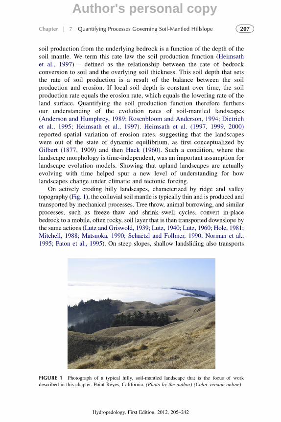
The steady-state distribution of 210Pbex in soils can be described by solvingthe traditional advection–diffusion model (e.g. DeMaster and Cochran, 1982),where the amount of 210Pbex in a particular volume of soil (A, in Bq cm�3) iscontrolled by the initial amount (A0), an advection term, which is defined hereas downward leaching of nuclides sorbed to colloidal materials, as expressedabove in Eqn (14). Radioactive equilibrium is a reasonable assumption at oursites: they have remained free from anthropogenic disturbance for at least 3half-lives of 210Pb, precipitation (which can control deposition) has remainedrelatively constant during the 20th century, and measured total inventories areconsistent with those predicted by deposition models. By modeling thedistribution of a single isotope in the soil column, it is not possible to solve forunique values of v and D, and it is unrealistic to ignore either leaching ordiffusion-like processes in soils. While our goal is to quantify D to measuresediment mixing, we need to constrain advection that might occur. For this, weuse the distribution of weapons-derived nuclides (137Cs and 241Am) in the soilprofile, which had a pulse-like input to soils during the 1950s and 1960s, witha strong global depositional maxima in 1963–1964 (US ERDA, 1977). Usingthe precise position of the subsurface concentration maxima of weapons-falloutin our soils, we determine v (Fig. 8).

While advection–diffusion models are the most common method fordescribing the depth distribution of fallout nuclides (Walling et al., 1999 andreferences therein), an alternative model for describing radionuclide




depth profiles may be required for sites that do not fall into the reasonably well-constrained conceptual framework outlined above. For example, inNewEngland (NE)>70% of the total 210Pbex inventory resides in organicmatterand the soils we examined showed no evidence of physical mixing. These,therefore, provided an important comparison with the well-mixed upland soilsthat are more typical for the landscapes selected for our work. Organic matterdecomposition must govern the concentration depth profiles of 210Pbex in Ohorizons to some extent, since the half-life of 210Pb is nearly an order ofmagnitude higher than the half-life or organic matter. As organic matterdecomposes, 210Pbex concentrations will increase from relative carbon loss. Amodified constant initial concentration (CIC) model (developed elsewhere forsedimentary environments; Appleby and Oldfield, 1992) can be applied to ourmeasured 210Pbex profiles, assuming that litterfall and 210Pb flux are relativelyconstant over time, and that the contribution of root mass in the O horizon isrelatively low. We posit that the only difference between the CIC model and ourdata is an exponential-based organic matter decomposition function. Thedecomposition functions that best explained our observed 210Pbex concentra-tion-depth profiles from NE can be evaluated using additional data on C cyclingdeveloped by others for similar forests (Currie and Aber, 1997; Berg, 2000).

We maximized the fit on the upper 15–20 cm of soil, the portion of the soilwith the majority of the nuclide inventory and the portion most likely to beinfluenced by organisms. At NR and TV, the advection–dispersion modeldescribed the 210Pbex profiles well, as total misplaced inventory was typically<18%. Dispersion coefficients can then be used to calculate mixing timeconstants s for a soil of thickness L (s¼ L2D�1). A soil 35 cm thick at NR is“turned over”, or mixed every 1200 y, and a similar thickness of soil at TV is

0 0.2 0.4 0.6

20

15

10

5

0

Bomb isotopes NRBomb isotopes NECosmogenic 7Be

Dep

th (c

m)

Activity (Bq cm-3, relative)

FIGURE 8 Depth profiles of cos-

mogenic 7Be and weapons-fallout

isotopes at New England (NE) and

Nunnock River, Bega Valley (BV)

field sites as described in Kaste et al.

(2007). 7Be is largely (>80%)

retained in the upper 2 cm of soil.

Weapons-fallout isotopes display

a sharp subsurface peak at NE

because of limited mixing; at BV,

similar isotopes are more dispersed

presumably from bioturbation. We

calculate v by using the position of

the subsurface maxima and assume

that it tracks the 1963 deposition

spike: v ranged from0.1 to 0.2 atNE,

and from 0.08 to 0.12 at BVandMC.




mixed every 660 y. If we use themixing timescale for a soil of 35-cm thickness atNR and assume that a particle travels 0.5 L during s, we calculate grain-scalevertical displacement velocities of 1–2 cmper century. Surprisingly, these valuesare relatively consistent with the 1–4 cm per century grain-scale velocitiescalculated at the same site by luminescence dating (Heimsath et al., 2002).

In contrast with NR and TV, a simple advection–dispersion model did notfit the data well in NE; our best model-data fits had misplaced inventory>30% (Fig. 9). In addition, the D values calculated here were on the order of1 cm2 y�1, a rate inconsistent with the preservation of the weapons spike(Fig. 8). Because the upper 5–10 cm of soil is the O horizon at our NE sites,which is usually >70% organic matter and very porous (~75%), the initialinfiltration of rainwater during intense storms could result in subsurface210Pbex peaks (Fig. 9c). Profiles of cosmogenic 7Be would capture this processwell because of its short half-life and its association with large rain events(Olsen et al., 1985). However, episodic vertical transport that might accom-pany intense precipitation events appears to be low at all three sites: 7Beactivity declines rapidly with depth and the upper 2 cm of soil typically retains>80% of the 7Be inventory (Fig. 8). 7Be was completely retained in the upper1–2 cm of soil at NR and TV.

Physical soil mixing rates determined with short-lived isotopes correlatewell with physical denudation rates measured by others (Fig. 10). Specifically,short-term soil mixing rates are highest at TV, where Heimsath et al. (1997)reported landscape denudation rates approaching 0.1 mm y�1 from cosmogenicnuclide analysis. On the other hand, physical denudation rates measured by

Pit 1 data

Pit 2 data

Pit 1 A-D model

Modeled D = 1.1 ± 0.3 cm2 y-1 Modeled D = 2.1 ± 0.4 cm2 y-1 Modeled D = 1.0 ± 0.3 cm2 y-1

0 0.1 0.2 0.3 0.4 0.1 0.2 0.3 0.4 0.50.50 0.1 0.2 0.3 0.4 0.5 0

Oi

Oe

Oa

E

Bs

Bw

0

5

10

15

20

25

Fraction of total 210Pbex inventory

Dep

th (c

m)

NETVNR

(a) (b) (c)

Pit 2 A-D model

Pit 1 data

Pit 2 data

Pit 1 A-D modelPit 2 A-D model

Pit 1 data

Pit 2 data

Pit 1 A-D modelPit 2 A-D model

FIGURE 9 210Pbex data and advection–diffusion (a–d) model given by Eqn (14); v was calculated

using weapons-derived isotopes (Fig. 8); we then solved for a D that best matched our data: 80–

90% agreement at BVand Point Reyes, Marin County (MC), sites of Heimsath et al. (2005), in NE

fits were typically <70%. Appendix 1 of Kaste et al. (2007) has more details on NE fits. Soil

horizons observed at New England shown on far right; no equivalent horizon boundaries exist at

Bega Valley and Marin County. Oi, fresh litter; Oe, moderately decomposed litter; Oa, humus; E,

strongly leached zone; Bs, zone with strong illuviation of iron oxides; Bw, chemically altered zone

with weak illuviation.




sediment traps in central NE are orders of magnitude lower (Likens andBormann, 1995), and we conclude from our nuclide profiles that short time-scale diffusion-like processes play a negligible role in mixing the soil layerhere. This suggests that relatively short-term soil mixing processes may limiterosion rates, and that there is a rough steady state between the continuousprocesses of soil mixing and long-term landscape evolution across contrastingfield settings. These results are interesting because tree-throw and landslides,which can occur episodically on timescales >100 y, are thought to bea significant sediment-transport mechanism (Dietrich et al., 2003). Because the210Pbex depth-concentration profiles are not described well with an A–D model,our work demonstrates quantitatively that freeze–thaw does not drive diffusion-like soil mixing in New England. The persistence of an insulating snowpackcover during the winter months probably minimizes the frequency of soilfreezing cycles here (Likens and Bormann, 1995). The presence of a fibrous,porous organic horizon in northern NE that undergoes short-term mixing onlyvia decomposition (and not random stirring) may protect mineral soil, andprobably limits physical denudation here. Using short-lived isotopes in this waydemonstrates quantitatively how process rates can vary in different geologicalsettings on a timescale that is traditionally difficult to capture. Furthermore, weshow that short-term diffusion-like processes are significant, and can play animportant role in landscape evolution and the fate of any element delivered tothe land surface.

4.4. Parent Material Strength

I now attempt to pull together all of the above results and discussion intoa final field-based measurement that is intended to provide a key mechanisticparameter for hillslope evolution. At several of our field sites, we used both

FIGURE 10 Short-term phys-

ical soil mixing rates calculated

in Kaste et al. (2007) vs. land-

scape denudation measured by

sediment traps and cosmogenic

isotopes inHeimsath et al. (1997;

2000). AmaximumD of 0.2 cm2

yr�1 forNEsoilswas determined

by using the shape of the 241Am

peak (plots similar to Fig. 7) and

an instantaneous pulse-like input

source assumption.




the cone penetrometer and the shear vane described above to quantify parentmaterial resistance to shear. Other studies explored the correlation betweenthese two instruments at different sites (Bachmann et al., 2006; Zimboneet al., 1996). Bachmann et al. specifically addressed the appropriateness ofusing a dynamic-cone penetrometer in soils to measure a horizontal shearstress that is a relative measure for the in situ strength state. The shear strengthof a soil is directly related to the normal stress applied (McKyes, 1989);therefore, an instrument that applies a force normal to the surface enables theestimate a relative shear strength. In fact, Bachmann et al. (2006) found thatthe vertically measured compression strength (strikes/cm) obtained at the finalsoil depth linearly related to the horizontal shear stress measured by the shearvane tester. We confirmed this with our own measurements and determineda linear fit between dynamic-cone penetrometer and shear vane testermeasurements that we used to convert strikes/cm from the cone penetrometerto kilopascals (Fig. 11).

Using both the shear vane and the cone penetrometer in soil pits dug acrossthree different field sites first reported elsewhere (Heimsath et al., 2000, 2005,2006, 2012), we quantify depth dependence for parent material strength(Fig. 12a). For each of the three field sites used for this aspect of our work, weoccupied the soil pits used for our cosmogenic nuclide and chemical weath-ering sampling studies and measured the competence of the parent materialimmediately beneath the mobile soil layer. The shallowest soils were observedin the rugged landscape of the San Gabriel Mountains, CA (SG) (Heimsathet al., 2012), where there is a relatively steep increase in parent materialstrength with increasing soil depth (black diamonds in Fig. 12a). Samples from

0

50

100

150

200

250

0 2 4 6 8

Shea

r stre

ngth

(kPa

)

Compressive Strength (strikes/cm)

FIGURE 11 Linear relation-

ship between shear vane tester

and dynamic-cone penetrom-

eter. Good linear fit confirms

principal stress theory such

that the vertically measured

compression strength (strikes/

cm) obtained at the final soil

depth is identical in size with

the horizontal shear stress

measured by the shear vane

tester. Green filled circles from

Byersdorfer (2006) and blue

filled diamonds from Johnson

(2008). Black line is fit to both

data sets, shear strength (kPa)¼32� compressive strength

(strikes/cm); R2¼ 0.86. (Color

version online)




the Nunnock River, Australia, site (Heimsath et al., 2000, 2006) (NR; redtriangles) overlay the SG measurements and the Point Reyes, California,samples (PR; blue circles) (Heimsath et al., 2005). Each of the three field sitesshows a distinct increase of parent material strength with increasing overlyingsoil thickness. Additionally, when taken together, these data suggest a broaderrelationship between parent material resistance to shear and the soil depth thatmantles the sample locations.

In related work that I did not expand upon in this chapter, we showed thatthe chemical weathering rates in saprolite decreased beneath increasing soilthicknesses (Burke et al., 2007, 2009). Those findings were counterintuitive toour observations of more highly weathered saprolite corresponding to thickeroverlying soil depths, but made sense when examined from the perspective thatthe higher soil production rates found beneath shallower soils should corre-spond to higher chemical weathering rates (Dixon et al., 2009a,b). The impacton physical weathering processes of the slower weathering rate beneath thickersoils is quantified with our measurements of parent material strength (Fig. 12a),and the observation of higher clay contents being found beneath thicker soils(Burke et al., 2009). We suggest that these higher clay contents and the moredeeply weathered saprolites (i.e. with higher chemical indices of alteration asdiscussed in Burke et al. (2007)) are actually more resistant to physical shear,

0

50

100

150

200

250

300

0 20 40 60 80 100 120 140

SG StrengthPR StrengthNR Strength

Stre

ngth

(kPa

)

Soil Depth (cm)

(a)

1

10

100

1000

0 50 100 150 200 250 300

PR Soil ProNR Soil ProSG Soil Pro2

Soil

Prod

uctio

n (m

/Ma)

Strength (kPa)

(b)

FIGURE 12 (a) Shear strength of the parent material beneath the active soil layer for three of the

field sites discussed here: San Gabriel Mountains (SG), California, described in DiBiase et al.

(2010) and Heimsath et al. (2012); Point Reyes (PR), California, just north of photograph in

Figure 1 and discussed in Heimsath et al. (2005); Nunnock River (NR), Bega Valley, Australia,

described initially in Heimsath et al. (2000) and several papers since then. Strength of the saprolite

is measured with both a shear vane and a cone penetrometer across the full range of soil depths –

strength vs. depth and increases across all sites with increasing soil thickness; (b) soil production

rates calculated with the soil production functions reported in Heimsath et al. (in review) for SG,

Heimsath et al. (2005 for PR) and Heimsath et al. (2000) for NR vs. the shear strength measured

beneath the same soil thicknesses as shown in (a). (Color version online)




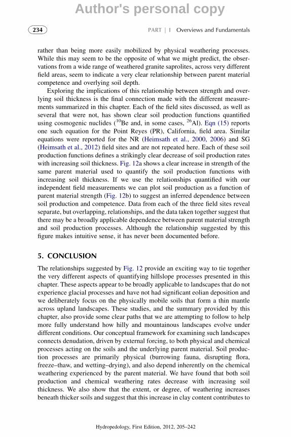
rather than being more easily mobilized by physical weathering processes.While this may seem to be the opposite of what we might predict, the obser-vations from a wide range of weathered granite saprolites, across very differentfield areas, seem to indicate a very clear relationship between parent materialcompetence and overlying soil depth.

Exploring the implications of this relationship between strength and over-lying soil thickness is the final connection made with the different measure-ments summarized in this chapter. Each of the field sites discussed, as well asseveral that were not, has shown clear soil production functions quantifiedusing cosmogenic nuclides (10Be and, in some cases, 26Al). Eqn (15) reportsone such equation for the Point Reyes (PR), California, field area. Similarequations were reported for the NR (Heimsath et al., 2000, 2006) and SG(Heimsath et al., 2012) field sites and are not repeated here. Each of these soilproduction functions defines a strikingly clear decrease of soil production rateswith increasing soil thickness. Fig. 12a shows a clear increase in strength of thesame parent material used to quantify the soil production functions withincreasing soil thickness. If we use the relationships quantified with ourindependent field measurements we can plot soil production as a function ofparent material strength (Fig. 12b) to suggest an inferred dependence betweensoil production and competence. Data from each of the three field sites revealseparate, but overlapping, relationships, and the data taken together suggest thatthere may be a broadly applicable dependence between parent material strengthand soil production processes. Although the relationship suggested by thisfigure makes intuitive sense, it has never been documented before.

5. CONCLUSION

The relationships suggested by Fig. 12 provide an exciting way to tie togetherthe very different aspects of quantifying hillslope processes presented in thischapter. These aspects appear to be broadly applicable to landscapes that do notexperience glacial processes and have not had significant eolian deposition andwe deliberately focus on the physically mobile soils that form a thin mantleacross upland landscapes. These studies, and the summary provided by thischapter, also provide some clear paths that we are attempting to follow to helpmore fully understand how hilly and mountainous landscapes evolve underdifferent conditions. Our conceptual framework for examining such landscapesconnects denudation, driven by external forcing, to both physical and chemicalprocesses acting on the soils and the underlying parent material. Soil produc-tion processes are primarily physical (burrowing fauna, disrupting flora,freeze–thaw, and wetting–drying), and also depend inherently on the chemicalweathering experienced by the parent material. We have found that both soilproduction and chemical weathering rates decrease with increasing soilthickness. We also show that the extent, or degree, of weathering increasesbeneath thicker soils and suggest that this increase in clay content contributes to




the increase in parent material competence observed beneath thicker soils. Thisincrease in competence corresponds to a decrease in soil production rates at thesame sites and we speculate that quantifying clay content more completely willlead to a more definitive connection.

Processes transporting the soil play an important role in connecting theincoming precipitation with the underlying parent material; namely, we haveused short-lived fallout-derived isotopes to quantify the physical mixingprocesses that are active across these landscapes. At all the sites where we havemade these measurements, we have documented a transition from dominantphysical mixing in the soil column to a dominance of overland flow withincreasing distance downslope. This transition from mixing to overland flowcorresponds to the transition from thin to thick soils because all of our field siteshave increasing soil depths downslope. The increase in overland flow processesdownslope may mean that the parent material beneath thicker soils is in contactwith soil water that has traveled farther through soil and is, therefore, not asable to weather as the water reacting with the parent material beneath thethinner, upslope soils. While this suggestion is speculative at best, it presentsa very clear link between hillslope hydrological processes acting across theselandscapes and the physical and chemical processes that I have summarized inthis chapter. If we can make all the observations presented in this chapter onlandscapes where the hillslope hydrology is well known, or vice versa, therewill be excellent opportunities to test this speculation and lead to a trulycomprehensive understanding of how upland landscapes evolve.

ACKNOWLEDGMENTS

This chapter reflects the enormous amount of work done by my graduate students over the last

decade. Jim Kaste helped hone and develop the short-lived isotope methodology applied here

to quantifying soil transport processes and rates. Ben Burke helped initiate the studies con-

necting soil production rates and processes with saprolite weathering. Jean Dixon took all

these methods further and integrated them with extensive work on quantifying the chemical

weathering signals on upland landscapes. Elizabeth Johnson and Joel Beyersdorfer lifted the

heavy cone penetrometer across many hillslopes and contributed to the strength studies.

Recent application of all of these methods in the San Gabriel Mountains benefited greatly

from the work of Roman DiBiase, Matt Jungers, and Josh Landis. My sincere thanks to all

of them.

REFERENCES

Ahnert, F., 1967. The role of the equilibrium concept in the interpretation of landforms of fluvial

erosion and deposition. In: Macar, P. (Ed.), L’evolution Des Versants. University of Liege,

Liege, pp. 23–41.

Ahnert, F., 1976. Brief description of a comprehensive three-dimensional process-response model

of landform development. Zeitschrift fur Geomorphologie, Supp. Band 25, 29–49.

Amundson, R., Richter, D.D., Humphreys, G.S., Jobbagy, E.G., Gaillardet, J., 2007. Coupling

between biota and earth materials in the critical zone. Elements 3 (5), 327–332.




Anderson, R.S., Humphrey, N.F., 1989. Interaction of weathering and transport processes in the

evolution of arid landscapes. In: Cross, T.A. (Ed.), Quantitative Dynamic Stratigraphy.

Prentice-Hall, Englewood Cliffs, N.J, pp. 349–361.

Anderson, R.S., 1994. Evolution of the santa cruz mountains, California, through tectonic growth

and geomorphic decay. J. Geophys. Res. Solid Earth 99 (B10), 20161–20179.

Anderson, R.S., 2002. Modeling the tor-dotted crests, bedrock edges, and parabolic profiles of high

alpine surfaces of the Wind River Range, Wyoming. Geomorphology 46, 35–58.

Anderson, S.P., Dietrich, W.E., 2001. Chemical weathering and runoff chemistry in a steep

headwater catchment. Hydrolog. Process. 15 (10), 1791–1815.

Anderson, S.P., Blum, J.D., Brantley, S.L., Chadwick, O., Chorover, J., Derry, L.A., Drever, J.I.,

Hering, J.G., Kirchner, J.W., Kump, L.R., Richter, D.D., White, A.F., 2004. Proposed

initiative would study earth’s weathering engine. EOS Trans. Am. Geophys. Union 85 (28),

265–269.

Anderson, S.P., von Blanckenburg, F., White, A.F., 2007. Physical and chemical controls on the

critical zone. Elements 3 (5), 315–319.

Appleby, P.G., Oldfield, F., 1992. Application of lead-210 to sedimentation studies. In:

Ivanovich, M., Harmon, R.S. (Eds.), Uranium-series Disequilibrium. Oxford University Press.

Bachmann, J., Contreras, K., Hartge, K.H., MacDonald, R., 2006. Comparison of soil strength

data obtained in situ with penetrometer and with vane shear test. Soil Tillage Res. 87, 112–

118.

Balco, G., Stone, J.O., Lifton, N.A., Dunai, T.J., 2008. A complete and easily accessible means of

calculating surface exposure ages or erosion rates from 10Be and 26Al measurements.

Quaternary Geochronology 3, 174–194.

Berg, B., 2000. Litter decomposition and organic matter turnover in northern forest soils. Forest

Ecol. Manag. 133, 13–22.

Bierman, P.R., 2004. Rock to sediment – slope to sea with Be-10 – rates of landscape change.

Annu. Rev. Earth Planet. Sci. 32, 215–255.

Black, T.A., Montgomery, D.R., 1991. Sediment transport by burrowing animals, Marin county,

California. Earth Surf. Process. Landforms 16, 163–172.

Bonniwell, E.C., Matisoff, G., Whiting, P.J., 1999. Determining the times and distances of particle

transit in a mountain stream using fallout radionuclides. Geomorphology 27, 75–92.

Brantley, S.L., Goldhaber, M.B., Ragnarsdottir, K.V., 2007. Crossing disciplines and scales to

understand the critical zone. Elements 3 (5), 307–314.

Braun, J., Heimsath, A.M., Chappell, J., 2001. Sediment transport mechanisms on soil-mantled

hillslopes. Geology 29, 683–686.

Brimhall, G.H., Dietrich, W.E., 1987. Constitutive mass balance relations between chemical

composition, volume, density, porosity, and strain in metasomatic hydrochemical systems:

results on weathering and pedogenesis. Geochim. Cosmochim. Acta 51, 567–587.

Brimhall, G.H., Chadwick, O.A., Lewis, C.J., Compston, W., Williams, I.S., Danti, K.J.,

Dietrich, W.E., Power, M.E., Hendricks, D., Bratt, J., 1992. Deformational mass transport and

invasive processes in soil evolution. Science 255, 695–702.

Brown, R.B., Cutshall, N.H., Kling, G.F., 1981a. Agricultural erosion indicated by Cs-137

redistribution 1. Levels and distribution of Cs-137 activity in soils. Soil Sci. Soc. Am. J. 45

(6), 1184–1190.

Brown, R.B., Kling, G.F., Cutshall, N.H., 1981b. Agricultural erosion indicated by Cs-137

redistribution. 2. Estimates of erosion rates. Soil Sci. Soc. Am. J. 45 (6), 1191–1197.

Burke, B.C., Heimsath, A.M., White, A.F., 2007. Coupling chemical weathering with soil

production across soil-mantled landscapes. Earth Surf. Process. Landforms 32, 853–873.




Burke, B.C., Heimsath, A.M., Dixon, J.L., Chappell, J., Yoo, K., 2009. Weathering the escarpment:

chemical and physical rates and processes, South-Eastern Australia. Earth Surf. Process.

Landforms 34, 768–785.

Burkins, D.L., Blum, J.D., Brown, K., Reynolds, R.C., Erel, Y., 1999. Chemistry and mineralogy

of a granitic, glacial soil chronosequence, Sierra Nevada Mountains, California. Chem. Geol.

162 (1), 1–14.

Buss, H.L., Brantley, S.L., Sak, P.B., White, A.F., 2004. Mineral dissolution at the grantie-saprolite

interface. In: Wanty, R.B., Seal, R.R.I. (Eds.), 11th International Symposium on Water-Rock

Interaction 11. Taylor and Francis, Saratoga Springs, NH, pp. 819–823.

Buss, H.L., Sak, P.B., Webb, S.M., Brantley, S.L., 2008. Weathering of the rio blanco quartz

diorite, Luquillo Mountains, Puerto Rico: Coupling oxidation, dissolution, and fracturing.

Geochim. Cosmochim. Acta 72, 4488–4507.

Byersdorfer, J.P., 2006. Correlating saprolite strength, soil production rate and chemical weath-

ering in granitic terrain: Point Reyes, CA and Nunnock River, Australia. MS Thesis, Dart-

mouth College, Department of Earth Sciences.

Cambray, R.S., Playford, K., Lewis, F.N.J., Carpenter, R.C., 1989. Radioactive Fallout in Air and

Rain: Results to the End of 1988. UK Atomic Energy Authority, Report no. AERE-R 10155,

Environ. Med. Sci. Div. Harwell Lab, Oxfordshire.

Carson, M.A., Kirkby, M.J., 1972. Hillslope Form and Process. Cambridge University Press,

New York, p. 475.

Cox, N.J., 1980. On the relationship between bedrock lowering and regolith thickness. Earth Surf.

Process. Landforms 5, 271–274.

Currie, W.S., Aber, J.D., 1997. Modeling leaching as a decomposition process in humid montane

forests. Ecology 78 (6), 1844–1860.

Dahlgren, R.A., Boettinger, J.L., Huntington, G.L., Amundson, R.G., 1997. Soil development

along an elevational transect in the western Sierra Nevada, California. Geoderma 78, 207–236.

DeMaster, D.J., Cochran, J.K., 1982. Particle mixing rates in deep-sea sediments determined from

excess 210Pb and 32Si profiles. Earth Planet. Sci. Lett. 61, 257–271.

DiBiase, R.A., Whipple, K.X., Heimsath, A.M., Ouimet, W.B., 2010. Landscape form and millennial

erosion rates in the San Gabriel Mountains, CA. Earth Planet. Sci. Lett. 289, 134–144.

Dietrich, W.E., Perron, J.T., 2006. The search for a topographic signature of life. Nature 439,

411–418.

Dietrich, W.E., et al., 2003. Geomorphic transport laws for predicting landscape form and

dynamics. In: Wilcock, P., Iverson, R. (Eds.), Prediction in Geomorphology. American

Geophysical Union, Washington, D.C, pp. 103–132.

Dietrich, W.E., Reiss, R., Hsu, M.-L., Montgomery, D.R., 1995. A process-based model for

colluvial soil depth and shallow landsliding using digital elevation data. Hydrolog. Process. 9,

383–400.

Dixon, J.L., Heimsath, A.M., Amundson, R., 2009a. The Critical Role of Climate and Saprolite

Weathering in Landscape Evolution. Earth Surf. Process. Landforms 34, 1507–1521.

Dixon, J.L., Heimsath, A.M., Kaste, J., Amundson, R., 2009b. Climate-driven processes of hill-

slope weathering. Geology 37, 975–978.

Dorr, H., 1995. Application of Pb-210 in Soils. J. Paleolimnol. 13 (2), 157–168.

Fleming, R.W., Johnson, A.M., 1975. Rates of seasonal creep of silty clay soil. Q. J. Eng. Geol.

8, 1–29.

Fletcher, R.C., Buss, H.L., Brantley, S.L., 2006. A spheroidal weathering model coupling pore-

water chemistry to soil thicknesses during steady-state denudation. Earth Planet. Sci. Lett.

244, 444–457.




Fornes, W.L., Whiting, P.J., Wilson, C.G., Matisoff, G., 2005. 137Cs-derived erosion rates in an

agricultural setting: the effects of model assumptions and management practices. Earth Surf.

Process. Landforms 30 (9), 1181–1189.

Frazier, C.S., Graham, R.C., 2000. Pedogenic transformation of fractured granitic bedrock,

southern California. Soil Sci. Soc. Am. J. 64, 2057–2069.

Furbish, D.J., 2003. Using the dynamically coupled behavior of land-surface geometry and soil

thickness in developing and testing hillslope evolution models. In: Wilcock, P., Iverson, R.

(Eds.), Prediction in Geomorphology, vol. 135. American Geophysical Union, Washington,

D.C, Geophysical Monograph, pp. 169–182.

Furbish, D.J., Haff, P.K., Dietrich, W.E., Heimsath, A.M., 2009. Statistical description of slope-

dependent soil transport and the diffusion-like coefficient. J. Geophys. Res. 114, F00A05,

doi: 10.1029/2009JF001267.

Gabet, E.J., 2000. Gopher bioturbation: field evidence for nonlinear hillslope diffusion. Earth Surf.

Process. Landforms 25, 1419–1428.

Gabet, E.J., Reichman, O.J., Seabloom, E.W., 2003. The effects of bioturbation on soil processes

and sediment transport. Ann. Rev. Earth Planet. Sci. 31, 249–273.

GEONOR, Instructions for Use, Inspection Vane Tester, H-60. GEONOR, INC, Milford, PA.

Available at http://www.geonor.com/field_vane_testing.html

Gilbert, G.K., 1877. Report on the Geology of the Henry Mountains (Utah). United States

Geological Survey, Washington, D.C.

Gilbert, G.K., 1909. The Convexity of Hilltops. Journal of Geology 17 (4), 344–350.

Green, E.G., Dietrich, W.E., Banfield, J.F., 2006. Quantification of chemical weathering rates

across an actively eroding hillslope. Earth Planet. Sci. Lett. 242, 155–169.

Hack, J.T., 1960. The interpretation of erosional topography in humid temperate regions.

Am. J. Sci. 258A, 80–97.

He, Q., Walling, D.E., 2003. Testing distributed soil erosion and sediment delivery models using

Cs-137 measurements. Hydrolog. Process. 17 (5), 901–916.

He, Q., Walling, D.E., 1996. Interpreting particle size effects in the adsorption of Cs-137

and unsupported Pb-210 by mineral soils and sediments. J. Environ. Radioact. 30 (2),

117–137.

Heimsath, A.M., 2006. Eroding the land: steady-state and stochastic rates and processes through

a cosmogenic lens. Geol. Soc. Am. Spec. Pap. 415, 111–129.

Heimsath, A.M., Chappell, J., Fifield, K., 2010. Eroding Australia: Rates and Processes from Bega

Valley to Arnhem Land. Geological Society, London. Special Publications, 346: 225–241.

Heimsath, A.M., Chappell, J., Dietrich, W.E., Nishiizumi, K., Finkel, R.C., 2000. Soil production

on a retreating escarpment in southeastern Australia. Geology 28, 787–790.

Heimsath, A.M., Chappell, J., Dietrich, W.E., Nishiizumi, K., Finkel, R.C., 2001a. Late Quaternary

erosion in southeastern Australia: a field example using cosmogenic nuclides. Quaternary Int.

83–5, 169–185.

Heimsath, A.M., Chappell, J., Finkel, R.C., Fifield, L.K., Alimanovic, A., 2006. Escarpment

erosion and landscape evolution in southeastern Australia. v. Penrose Conference Series. Geol.

Soc. Am. Spec. Pap. 398, 173–190.

Heimsath, A.M., Chappell, J., Spooner, N.A., Questiaux, D., 2002. Creeping soil. Geology 30,

111–114.

Heimsath, A.M., Dietrich, W.E., Nishiizumi, K., Finkel, R.C., 1997. The soil production function

and landscape equilibrium. Nature 388, 358–361.

Heimsath, A.M., Dietrich, W.E., Nishiizumi, K., Finkel, R.C., 1999. Cosmogenic nuclides,

topography, and the spatial variation of soil depth. Geomorphology 27, 151–172.




Heimsath, A.M., Dietrich, W.E., Nishiizumi, K., Finkel, R.C., 2001b. Stochastic processes of soil

production and transport: erosion rates, topographic variation, and cosmogenic nuclides in the

Oregon coast range. Earth Surf. Process. Landforms 26, 531–552.

Heimsath, A.M., Furbish, D.J., Dietrich, W.E., 2005. The illusion of diffusion: field evidence for

depth-dependent sediment transport. Geology 33, 949–952.

Heimsath, A.M., Hancock, G.R., Fink, D., 2009. The ‘humped’ soil production function: eroding

Arnhem Land, Australia. Earth Surf. Process. Landforms 34, 1674–1684.

Heimsath, A.M., DiBiase, R.A., Whipple, K.X., 2012. Soil production limits and the transition to

bedrock dominated landscapes. Nature Geoscience 5 (5), 210–214.

Herrick, J.E., Jones, T.L., 2002. A dynamic cone penetrometer for measuring soil penetration

resistance. Soil Sci. Soc. Am. J. 66, 1320–1324.

Hole, F.D., 1981. Effects of animals on soil. Geoderma 25, 75–112.

Jiao, J.J., Wang, X.-S., Nandy, S., 2005. Confined groundwater zone and slope instability in

weathered igneous rocks in Hong Kong. Eng. Geol. 80, 71–92.

Johnson-Maynard, J., Anderson, M.A., Green, S., Graham, R.C., 1994. Physical and hydraulic-

properties of weathered granitic rock in Southern California. Soil Sci. 158 (5), 375–380.

Johnson, E.R., 2008. Rocks Matter: Exploring the Intersection of Lithology and Tectonics.

MS Thesis, Dartmouth College Department of Earth Sciences.

Jones, D.P., Graham, R.C., 1993. Water-holding characteristics of weathered granitic rock in

chaparral and forest ecosystems. Soil Sci. Soc. Am. J. 57 (1), 256–261.

Kaste, J.M., Heimsath, A.M., Bostick, B.C., 2007. Short-term soil mixing quantified with fallout

radionuclides. Geology 35, 243–246.

Kaste, J.M., Heimsath, A.M., Hohmann, M., 2006. Quantifying sediment transport across an

undisturbed prairie landscape using cesium-137 and high resolution topography. Geomor-

phology 76, 430–440.

Kew, G., Gilkes, R., 2006. Classification, strength and water retention characteristics of lateritic

regolith. Geoderma 136, 184–198.

Lal, D., 1991. Cosmic ray labeling of erosion surfaces: in situ nuclide production rates and erosion

models. Earth Planet. Sci. Lett. 104, 424–439.

Lamb, M.P., Scheingross, J.S., Amidon, W.H., Swanson, E., Limaye, A., 2011. A Model for

Fire-Induced Sediment Yield by Dry Ravel in Steep Landscapes. J. Geophys. Res. 116,

F03006, doi:10.1029/2010JF001878.

Lebedeva, M.I., Fletcher, R.C., Balashov, V.N., Brantley, S.L., 2007. A reactive diffusion model

describing transformation of bedrock to saprolite. Chem. Geol. 244, 624–645.

Likens, G.E., Bormann, F.H., 1995. Biogeochemistry of a Forested Ecosystem. Springer-Verlag,

New York, p. 160.

Lowrance, R., McIntyre, S., Lance, C., 1988. Erosion and deposition in a field forest system

estimated using cesium-137 activity. J. Soil Water Conservat. 43 (2), 195–199.

Lutz, H.J., Griswold, F.S., 1939. The influence of tree roots on soil morphology. Am. J. Sci. 258,

389–400.

Lutz, H.J., 1940. Disturbance of forest soil resulting from the uprooting of trees. Bull. Yale Univ.

Sch. Forest 45, 1–37.

Lutz, H.J., 1960. Movement of rocks by uprooting of forest trees. Am. J. Sci. 258, 752–756.

Matisoff, G., Bonniwell, E.C., Whiting, P.J., 2002a. Radionuclides as indicators of sediment

transport in agricultural watersheds that drain to Lake Erie. J. Environ. Qual. 31 (1), 62–72.

Matisoff, G., Bonniwell, E.C., Whiting, P.J., 2002b. Soil erosion and sediment sources in an

Ohio watershed using beryllium-7, cesium-137, and lead-210. J. Environ. Qual. 31 (1),

54–61.




Matisoff, G., Ketterer, M.E., Wilson, C.G., Layman, R., Whiting, P.J., 2001. Transport of rare earth

element-tagged soil particles in response to thunderstorm runoff. Environ. Sci. Technol. 35

(16), 3356–3362.

Matsuoka, N., 1990. The rate of bedrock weathering by frost action: field measurements and

a predictive model. Earth Surf. Process. Landforms 15, 73–90.

Matsuoka, N., Moriwaki, K., 1992. Frost heave and creep in the sor rondane mountains. Arctic

Antarct. Alpine Res. 24, 271–280.

McKean, J.A., Dietrich, W.E., Finkel, R.C., Southon, J.R., Caffee, M.W., 1993. Quantification of

soil production and downslope creep rates from cosmogenic 10Be accumulations on a hillslope

profile. Geology 21 (4), 343–346.

McKyes, E., 1989. Agricultural Engineering Soil Mechanics. In: Developments in Agricultural

Engineering, vol. 10. Elsevier, Amsterdam, p. 292.

Minasny, B., McBratney, A.B., 1999. A rudimentary mechanistic model for soil production and

landscape development. Geoderma 90 (1–2), 3–21.

Minasny, B., McBratney, A.B., 2001. A rudimentary mechanistic model for soil formation and

landscape development II. A two-dimensional model incorporating chemical weathering.

Geoderma 103, 161–179.

Mitchell, P., 1988. The influences of vegetation, animals and micro-organisms on soil processes.

In: Viles, H.A. (Ed.), Biogeomorphology. Basil Blackwell, New York, pp. 43–82.

Montgomery, D.R., 2007. Soil erosion and agricultural sustainability. Proc. Natl. Acad. Sci. U S A

104 (33), 13268–13272.

Mudd, S.M., Furbish, D.J., 2006. Using chemical tracers in hillslope soils to estimate the

importance of chemical denudation under conditions of downslope sediment transport.

J. Geophys. Res. Earth Surf. 111 (F2).

Norman, S.A., Schaetzl, R.J., Small, T.W., 1995. Effects of slope angle on mass movements by tree

uprooting. Geomorphology 14, 19–27.

O’Farrell, C.R., Heimsath, A.M., Kaste, J.M., 2007. Quantifying hillslope erosion rates and

processes for a coastal California landscape over varying timescales. Earth Surf. Process.

Landforms 32, 544–560.

Olsen, C.R., et al., 1985. Atmospheric fluxes and marsh-soil inventories of Be-7 and Pb-210.

J. Geophys. Res. Atmos. 90 (ND6), 487–495.

Paton, T.R., Humphries, G.S., Mitchell, P.B., 1995. Soils: A New Global View. UCL Press

Limited, London, p. 213.

Pelletier, J.D., Rasmussen, C., 2009. Quantifying the climatic and tectonic controls on hillslope

steepness and erosion rate. Lithosphere 1, 73–80.

Porto, P., Walling, D.E., Tamburino, V., Callegari, G., 2003. Relating caesium-137 and soil loss

from cultivated land. Catena 53 (4), 303–326.

Prosser, I.P., Dietrich, W.E., 1995. Field experiments on erosion by overland flow and their

implication for a digital terrain model of channel initiation. Water Resour. Res. 31, 2867–2876.

Quine, T.A., Govers, G., Walling, D.E., Zhang, X.B., Desmet, P.J.J., Zhang, Y.S., Vandaele, K.,

1997. Erosion processes and landform evolution on agricultural land – new perspectives from

caesium-137 measurements and topographic-based erosion modelling. Earth Surf. Process.

Landforms 22 (9), 799–816.

Reneau, S.L., Dietrich, W.E., 1990. Depositional history of hollows on steep hillslopes, coastal

Oregon and Washington. Natl. Geogr. Res. 6 (2), 220–230.

Reneau, S.L., Dietrich, W.E., 1991. Erosion rates in the southern oregon coast range: evidence for

an equilibrium between hillslope erosion and sediment yield. Earth Surf. Process. Landforms

16 (4), 307–322.




Riebe, C.S., Kirchner, J.W., Finkel, R.C., 2003a. Long-term rates of chemical weathering and

physical erosion from cosmogenic nuclides and geochemical mass balance. Geochim.

Cosmochim. Acta 67, 4411–4427.

Riebe, C.S., Kirchner, J.W., Finkel, R.C., 2003b. Sharp decrease in long-term chemical weathering

rates along an altitudinal transect. Earth Planet. Sci. Lett. 6393, 1–14.

Riebe, C.S., Kirchner, J.W., Finkel, R.C., 2004. Erosional and climatic effects on long-term

chemical weathering rates in granitic landscapes spanning diverse climate regimes. Earth

Planet. Sci. Lett. 224, 547–562.

Riebe, C.S., Kirchner, J.W., Granger, D.E., Finkel, R.C., 2000. Erosional equilibrium and

disequilibrium in the Sierra Nevada, inferred from cosmogenic Al and Be in alluvial sediment.

Geology 28, 803–806.

Riebe, C.S., Kirchner, J.W., Granger, D.E., Finkel, R.C., 2001a. Minimal climatic control on

erosion rates in the Sierra Nevada, California. Geology 29, 447–450.

Riebe, C.S., Kirchner, J.W., Granger, D.E., Finkel, R.C., 2001b. Strong tectonic and weak climatic

control of long-term chemical weathering rates. Geology 29, 511–514.

Roels, J.M., 1985. Estimation of soil loss at a regional scale based on plot measurements – some

critical considerations. Earth Surf. Process. 10, 587–595.

Roering, J.J., Almond, P., Tonkin, P., McKean, J., 2002. Soil transport driven by biological

processes over millenial time scales. Geology 30 (12), 1115–1118.

Roering, J.J., Gerber, M., 2005. Fire and the evolution of steep, soil-mantled landscapes. Geology

33, 349–352.

Roering, J.J., Kirchner, J.W., Dietrich, W.E., 1999. Evidence for non-linear, diffusive sediment trans-

port on hillslopes and implications for landscapemorphology.WaterResour. Res. 35 (3), 853–870.

Roering, J.J., Kirchner, J.W., Sklar, L.S., Dietrich, W.E., 2001. Hillslope evolution by nonlinear

creep and landsliding: an experimental study. Geology 29, 143–146.

Rosenbloom, N.A., Anderson, R.S., 1994. Hillslope and channel evolution in a marine terraced

landscape, Santa Cruz, California. J. Geophys. Res. 99 (B7), 14,013–14,029.

Schaetzl, R.J., Follmer, L.R., 1990. Longevity of treethrow microtopography: implications for

mass wasting. Geomorphology 3, 113–123.

Schoeneberger, P.J., Amoozegar, A., Buol, S.W., 1995. Physical property variation of a soil and

saprolite continuum at 3 geomorphic positions. Soil Sci. Soc. Am. J. 59 (5), 1389–1397.

Selby, M.J., 1980. A rock mass strength classification for geomorphic purposes: with tests from

Antarctica and New Zealand. Zeitschrift fur Geomorphologie N. F. 24 (1), 31–51.

Selby, M.J., 1985. Hillslope Materials and Processes. Oxford University Press, Oxford, England.

Simon, S.L., Bouville, A., Beck, H.L., 2004. The geographic distribution of radionuclide depo-

sition across the continental US from atmospheric nuclear testing. J. Environ. Radioact. 74

(1–3), 91–105.

Steegen, A., Govers, G., Takken, I., Nachtergaele, J., Poesen, J., Merckx, R., 2001. Factors

controlling sediment and phosphorus export from two Belgian agricultural catchments.

J. Environ. Qual. 30 (4), 1249–1258.

Tyler, A.N., Carter, S., Davidson, D.A., Long, D.J., Tipping, R., 2001. The extent and significance

of bioturbation on Cs-137 distributions in upland soils. Catena 43 (2), 81–99.

U.S. ERDA (United States Energy Research and Development Administration), 1977, Final

Tabulation of Monthly 90Sr Fallout Data: 1954–1976: New York, Environmental Measure-

ments Laboratory, Report HASL-329.

Viles, H., A., Goudie, A., Grab, S., Lalley, J., 2011. The use of the schmidt hammer and equotip

for rock hardness assessment in geomorphology and heritage science: a comparative analysis.

Earth Surf. Process. Landforms 36, 320–333.




Wallbrink, P.J., Murray, A.S., 1996. Distribution and variability of Be-7 in soils under different

surface cover conditions and its potential for describing soil redistribution processes. Water

Resour. Res. 32 (2), 467–476.

Walling, D.E., He, Q., 1999. Using fallout lead-210 measurements to estimate soil erosion on

cultivated land. Soil Sci. Soc. Am. J. 63 (5), 1404–1412.

Walling, D.E., He, Q., Blake, W., 1999. Use of Be-7 and Cs-137 measurements to document short-

and medium-term rates of water-induced soil erosion on agricultural land. Water Resour. Res.

35 (12), 3865–3874.

Walling, D.E., Russell, M.A., Hodgkinson, R.A., Zhang, Y., 2002. Establishing sediment budgets

for two small lowland agricultural catchments in the UK. Catena 47 (4), 323–353.

West, A., Galy, A., Bickle, M., 2005. Tectonic and climatic controls on silicate weathering. Earth

and Planetary Science Letters 235 (1–2), 211–228.

White, A.F., Brantley, S.L., 2003. The effect of time on the weathering of silicate minerals: why do

weathering rates differ in the laboratory and field? Chem. Geol. 202 (3–4), 479–506.

White, A.F., Blum, A.E., Schulz, M.S., Bullen, T.D., Harden, J.W., Peterson, M.L., 1996.

Chemical weathering rates of a soil chronosequence on granitic alluvium. 1. Quantification of

mineralogical and surface area changes and calculation of primary silicate reaction rates.

Geochim. Cosmochim. Acta 60 (14), 2533–2550.

Whiting, P.J., Bonniwell, E.C., Matisoff, G., 2001. Depth and areal extent of sheet and rill erosion

based on radionuclides in soils and suspended sediment. Geology 29, 1131–1134.

Wilson, C.G., Matisoff, G., Whiting, P.J., 2003. Short-term erosion rates from a Be-7 inventory

balance. Earth Surf. Process. Landforms 28 (9), 967–977.

Yoo, K., Amundson, R., Heimsath, A.M., Dietrich, W.E., Brimhall, G.H., 2007. Integration of

geochemical mass balance with sediment transport to calculate rates of soil chemical

weathering and transport on hillslopes. J. Geophys. Res. Earth Surf. 112 (F2).

Young, A., 1960. Soil movement by denudational processes on slopes. Nature 188, 120–122.

Young, A., 1963. Some field observations of slope form and regolith, and their relation to slope

development. Trans. Inst. Br. Geogr. 32, 1–29.

Zhang, X.B., Quine, T.A., Walling, D.E., Li, Z., 1994. Application of the cesium-137 technique in

a study of soil-erosion on gully slopes in a yuan area of the loess plateau near Xifeng, Gansu

Province, China. Geogr. Ann. Phys. Geogr. 76 (1–2), 103–120.

Zimbone, S.M., Vickers, A., Morgan, R.P.C., Vella, P., 1996. Field investigations of different

techniques for measuring surface soil shear strength. Soil Technol. 9 (1–2), 101–111.




Documents

Author's personal copy › ~aheimsat › publications › Heimsath... · (Anderson and Humphrey, 1989; Rosenbloom and Anderson, 1994; Dietrich et al., 1995; Heimsath et al., 1997)