AutoLanding Controller for a Fixed Wing Unmanned Air Vehiclewelcome.isr.tecnico.ulisboa.pt/wp-content/uploads/2015/05/1742... · Autolanding Controller for a Fixed Wing Unmanned Air

Autolanding Controller for a Fixed Wing Unmanned

Air Vehicle

Paulo Rosa∗, Carlos Silvestre†, David Cabecinhas‡, Rita Cunha§

Instituto Superior Tecnico, Institute for Systems and Robotics, 1049-001 Lisbon, Portugal

This paper addresses the autolanding guidance and control problem for unmanned au-tonomous vehicles (UAV) based on the information provided by the onboard NavigationSystem. The proposed solution relies on a path-following and velocity profile tracking con-troller synthesized using an accurate aircraft dynamic model, referred to as SymAirDyn,which was designed with the objective of exploiting the whole aircraft’s flight envelope. Asuitable polytopic Linear Parameter Varying (LPV) representation with piecewise affinedependence on the parameters is adopted to accurately model the desired aircraft dy-namics over a set of predefined operating regions. The synthesis problem is stated as acontinuous-time H2 control problem for LPV systems and solved using Linear Matrix In-equalities (LMIs). During the controller design stage, the aircraft landing maneuver isdecomposed in the two standard phases: the glideslope and the flare. For each phase, therequired control objectives are identified and specific controllers are designed. The con-troller implementation is tackled within the framework of gain-scheduling control theoryusing the D-methodology. The performance and effectiveness of the resulting nonlineargain scheduling controller is illustrated in simulation, using the nonlinear model SymAir-

Dyn under different types of disturbances, namely Dryden spectrum generated wind duringthe glideslope and wind gusts near touchdown.

I. Introduction

Over the last decade, the advent of new sensor technology and the successes of already deployed platformshave bolstered a worldwide interest on developing and expanding the capabilities of Unmanned Air Vehicles(UAVs). A remarkably wide spectrum of UAV configurations is currently in use or under development,ranging from fixed and rotary wing, going from micro to jet-sized. Fixed wing UAVs are already beingused in commercial applications such as rice fields spraying and fish banks search in Japan. Companieslike Scandicraft, Schiebel and Yamaha have industrial helicopters available for filming operations in risksituations. Other applications that are currently being brought forward include maintenance and securityinspection of power lines, and oil and gas pipelines; forest fire surveillance; environmental observation andmonitoring of natural disaster areas; among others.

The advent of new empowering stand-alone sensors, such as the Laser Range Finder and GPS hasencouraged the adoption of onboard positioning and enhanced the navigation systems. These systems arecurrently recognized as instrumental in bringing about all the capabilities of an UAV to perform high precisiontasks in challenging and uncertain operation scenarios. Several different methods have been proposed andflight tested,1–3 confirming the expected robustness and performance that can be achieved in the executionof specific maneuvers, such as landing or steering the vehicle to a desired target.

Nowadays airports are equipped with runway approaching systems that provide lateral and verticalguidance to aircrafts during the glideslope and final landing maneuver. A common mechanism is the so-calledInstrument Landing System (ILS)4 that is composed of several radio beacons placed on the runway, allowingfor vertical and lateral accurate guidance of the aircraft during the landing phase. Once the approaching

∗PhD Student, Department of Electrical Engineering and Computer Science (DEEC), Av. Rovisco Pais 1;[email protected].

†Assistant Professor, DEEC, Av. Rovisco Pais 1; [email protected]. Member AIAA.‡PhD Student, DEEC, Av. Rovisco Pais 1; [email protected].§PhD Student, DEEC, Av. Rovisco Pais 1; [email protected].

1 of 22

American Institute of Aeronautics and Astronautics

AIAA Guidance, Navigation and Control Conference and Exhibit20 - 23 August 2007, Hilton Head, South Carolina

AIAA 2007-6770

Copyright © 2007 by the American Institute of Aeronautics and Astronautics, Inc. All rights reserved.

maneuver starts, the ILS guides the vehicle to a certain height, referred to as the decision height, whichdepends on the airport’s ILS category and on the ILS based guidance system available onboard the aircraft.Different ILS categories provide different levels of autonomy to the aircraft runway approach and landingsystem. The most advanced one, ILS Category IIIc, allows for the automatization of the entire maneuverincluding guidance along the runway. Despite the availability of those advanced landing systems, theircomplexity and the high cost involved on their implementation turn them into prohibitive solutions for smallUAVs which should be able to land on any opportunity runway, grassy strip, or available road, resortingto low cost onboard navigation systems.5 These systems provide the vehicle’s automatic landing guidanceand control algorithms with the actual vehicle’s linear and angular positions and velocities, and dedicatedmodules allow for the integration of GPS/INS information with height data as acquired by a Radar Altimeteror Laser Range Finder mounted underneath the aircraft.

In this paper, the autolanding guidance and control problem is addressed along the lines of the workreported in Refs. 6, 7, and in a companion paper on path following control for coordinated turn maneuvers,Ref. 8, while having in mind the high precision requirements involved in the design of guidance and controllaws for the terminal approach and landing maneuvers of fixed wing aircrafts. The proposed solution totackle the autolanding guidance and control system design problem is a path-following velocity-trackingtechnique9 that relies on the definition of a path-dependent error space to express the dynamic model ofthe aircraft. The error vector, which the autolanding controller should drive to zero, comprises velocityerrors, orientation errors, and the distance to the desired path along the different landing phases, defined asthe distance between the actual vehicle’s position and its orthogonal projection on the path. For differentapproaches to the problem, the interested reader is referred to Ref. 10, which discusses a landing angleestimation algorithm in UAV autolanding simulation, Ref. 11, where the authors investigate the use ofneural networks with linearized inverse aircraft model in automatic landing systems, and to Ref. 12, thatpresents a mixedH2/H∞ controller design for autolanding systems with application to a commercial airplane.

The design and implementation of high-precision robust guidance and control algorithms is one of the keyelements in the development of reliable UAV systems. Several approaches to the problem have been proposed,including robust linear control, nonlinear control, neural networks, and fuzzy control – see for exampleRefs. 13, 14 and references therein. Nonlinear approaches rely on feedback linearization and backsteppingtechniques, which require the aircraft dynamic model to be approximated by an input-output linearizablesystem. Linear Parameter Varying (LPV) models represent nowadays a compromise between the globalaccuracy of nonlinear models and the straightforward controller synthesis techniques available for LinearTime Invariant (LTI) representations. It is well-known that LPV models used within the framework of gain-scheduling constitute a powerful tool for tackling difficult nonlinear problems.15, 16 In the present design, apolytopic LPV representation with piecewise affine dependence on the parameters is adopted to accuratelymodel the desired aircraft dynamics over a set of predefined operating regions. Using an Linear MatrixInequalities (LMIs) approach and based on the concept of quadratic stability for LPV systems, this paperaddresses the autolanding controller synthesis problem in a systematic way and derives in a straightforwardmanner H2 controllers for the selected operating regions. The resulting set of nonlinear controllers areimplemented resorting to the so called D-methodology17 thereby eliminating the need to feedforward thetrimming values for the actuation signals and outputs.

In order to design and evaluate the performance of the autolanding controller, a simulation model ofthe aircraft dynamics named SimAirDyn, is introduced. SimAirDyn implements, in the MATLAB Simulinkenvironment, a dynamic model for fixed wing aircrafts valid over a wide flight envelope. The model wasderived from first-principles for effective control system design and simulation. The airplane is modeled asa six degrees of freedom rigid body, actuated by forces and moments that are generated at the propeller,fuselage, wings, empennage and control surfaces. The remaining components, such as the landing gear andthe antennas, which have a smaller impact on the overall behavior of the aircraft dynamic model, are notincluded in the simulator and will be treated as disturbances by the control system. Several reference bookson the theory of fixed wing aircraft flight dynamics can be found in the literature. The reader is referred toRef. 18 and Ref. 19 for a thorough and extensive coverage of full-scale aircraft dynamic modeling. Previouswork on aircraft flight dynamics identification can be found in Ref. 20 where the authors treat parameteridentification issues for nonlinear multivariable aircraft models and report results on the convergence analysisof the proposed identification algorithm.

The paper is organized as follows. Section II presents SimAirDyn, a simulation based on the standardrigid-body dynamic model, which can be used to describe autonomous air vehicles; Section III introduces

2 of 22


the path-dependent error space for each stage of the landing maneuver, presents a derivation of the errordynamics parameterized by a vector that fully characterizes the desired operating point, and particularizes forthe case of airplanes, introducing a reduced parameter vector and a suitable error output vector; Section IVreviews theoretical results on LPV systems and presents the strategy adopted to guide and control thevehicle; simulation results obtained with the full nonlinear model of an UAV are presented in Section V.

II. Vehicle Dynamic Model

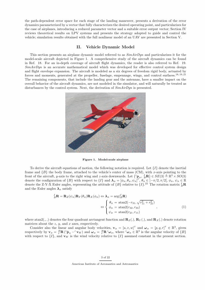
This section presents an airplane dynamic model referred to as SimAirDyn and particularizes it for themodel-scale aircraft depicted in Figure 1. A comprehensive study of the aircraft dynamics can be foundin Ref. 18. For an in-depth coverage of aircraft flight dynamics, the reader is also referred to Ref. 19.SimAirDyn is an accurate mathematical model which was developed for effective control system designand flight envelope expansion. The aircraft is modeled as a six degrees of freedom rigid body, actuated byforces and moments, generated at the propeller, fuselage, empennage, wings, and control surfaces.18, 19, 21

The remaining components, that include the landing gear and the antennas, have a smaller impact on theoverall behavior of the aircraft dynamics, are not modeled in the simulator, and will naturally be treated asdisturbances by the control system. Next, the derivation of SimAirDyn is presented.

Figure 1. Model-scale airplane

To derive the aircraft equations of motion, the following notation is required. Let {I} denote the inertialframe and {B} the body frame, attached to the vehicle’s center of mass (CM), with x-axis pointing to thefront of the aircraft, y-axis to the right wing and z-axis downwards. Let

(

IpB, I

BR)

∈ SE(3) , R3 × SO(3)denote the configuration of {B} with respect to {I} and λB = [φB , θB, ψB]

T, θB ∈ ]−π/2, π/2[, φB , ψB ∈ R

denote the Z-Y-X Euler angles, representing the attitude of {B} relative to {I}.22 The rotation matrix IBR

and the Euler angles λB satisfy

IBR = RZ(ψB)RY (θB)RX(φB) ⇔ λB = arg(I

BR)

⇔

θB = atan2(−r31,√

r211 + r221)

φB = atan2(r32, r33)

ψB = atan2(r21, r11)

, (1)

where atan2(., .) denotes the four quadrant arctangent function and RZ(.), RY (.), and RX(.) denote rotationmatrices about the z, y, and x axes, respectively.

Consider also the linear and angular body velocities, vB = [u, v, w]T and ωB = [p, q, r]T ∈ R3, givenrespectively by vB = B

I R (IpB−I vW ) and ωB = B

I R IωB , where IωB ∈ R3 is the angular velocity of {B}with respect to {I}, and vW is the wind velocity relative to {I} assumed constant in the present section.

3 of 22


According to this notation, the standard equations for the vehicle’s kinematics22 can be written as

{

IpB

= IBRvB + vW

λB = Q(φB , θB)ωB

, (2)

where

Q(φB , θB)=

1 sinφB tan θB cosφB tan θB

0 cosφB − sinφB

0 sinφB/cos θB cosφB/cos θB

, (3)

and the derivative of IBR is given by

IBR = I

BRS(ωB), (4)

where S(x) ∈ R3×3 is a skew symmetric matrix such that S(x)y = x × y, for all x, y ∈ R3. The dynamicmodel of the vehicle can be written as

{

vB = f (vB,ωB ,u, θB, φB)

ωB = n(vB ,ωB,u, θB, φB), (5)

where f , n : (R3,R3,Rm,R,R) → R3 are continuously differentiable functions of the body velocities, attitudeand control inputs u ∈ Rm that derive from the remaining forces and moments acting on the body. Furtherdefine the aircraft airspeed, V , the angle-of-attack, AOA, α = arctan(w/u), and the angle of sideslip β =arcsin(v/V ).

The overall model resulting from the integration of the above mentioned components is a highly coupledMIMO nonlinear dynamic system. However, analysis of the mission objectives will help to establish therelevant flight regimes, such as forward flight, coordinated turn, take-off, and landing, whose independentmodeling can yield simpler and more effective and intuitive dynamic systems. This paper will give particularfocus to the landing maneuver.

A standard procedure in the literature is to separate the aircraft into longitudinal and lateral-directionaldynamics. This manipulation leads to a simpler analysis and to a clearer and intuitive interpretation of theresults. The full derivation of the longitudinal and lateral-directional dynamics can be found in Ref. 18.

A. Aircraft Model Description

The resulting dynamic systems for both the full nonlinear model and the simplified models are expressed instate-space form and were used to develop a realistic aircraft simulation model using MATLAB/Simulink.The simplified models for the different flight regimes were validated against the full nonlinear aircraft simu-lation model, providing the working ground for the control design phase.

The aircraft nonlinear simulation model SimAirDyn was properly tuned so that it captures the essentialbehavior of the actual vehicle for a large operational flight envelope.18, 19 The most important model param-eters are the dimensionless aerodynamic force and torque coefficients, which can be obtained from a Taylorseries expansion about selected operating regimes.19 Typically these values are experimentally obtained in awind tunnel. Alternatively, software packages exist that allow one to obtain reasonably good approximationsof wind-tunnel experiments. One of these software packages is LinAir 4 from Desktop Aeronautics, whichwas purchased by ISR/IST. LinAir 4 is an aircraft geometry modeler that provides a wide range of compu-tational aerodynamic analysis, based on the calculation of the aerodynamic characteristics of multi-element,nonplanar lifting surfaces. The methodology used to derive the nonlinear dynamic model parameters fromthe aerodynamic loads estimated by LinAir 4 was based on the relation between the system responses andthe relative interplay of physical quantities.

f(vB,ωB,uad, θB, φB) = fad(vB,ωB,uad) + fg(θB, φB) +[

T 0 0]T

n(vB,ωB,uad, θB, φB) = nad(vB ,ωB,uad)(6)

As expressed in eq. (6), the external forces and moments acting on the rigid body can be separated intogravity, fg(θB, φB), airflow acting on the fuselage, wings, empennage and control surfaces, fad(vB,ωB,uad)

4 of 22


and nad(vB,ωB,uad), and the force exerted by the propeller [T, 0 0]T . The gravitational terms can betrivially computed from the attitude of the aircraft, while the remaining ones were obtained using a leastsquare fitting from data generated by LinAir 4. In (6), uad = [δaL

, δaR, δr, δe, δf ]T represents the vector of

control inputs, where δaL, δaR

, δr, δe, δf are the deflection angles of left and right ailerons, rudder, elevator,and flaps, respectively. The main problems addressed were the development of a reliable strategy for nonlinearmodel structure and parameter identification from data produced by LinAir 4 and the selection of a set ofaircraft maneuvers and control surface configurations to cover the aircraft flight envelope. The aerodynamicforces and moments acting on the airframe were evaluated for several flight conditions and then interpolatedusing a least square fitting to obtain the aircraft dynamic model for the whole flight envelope.

The model was tuned for the aircraft presented in Figure 1. This aircraft is capable of lifting a 11 kgpayload for two hours on a tank of gas. The wingspan is 3.5 m and the length is 1.8 m, and it has a takeoffdistance half loaded of 50 m. It uses a one cylinder two stroke-60 cc engine, producing about 8 horsepower.

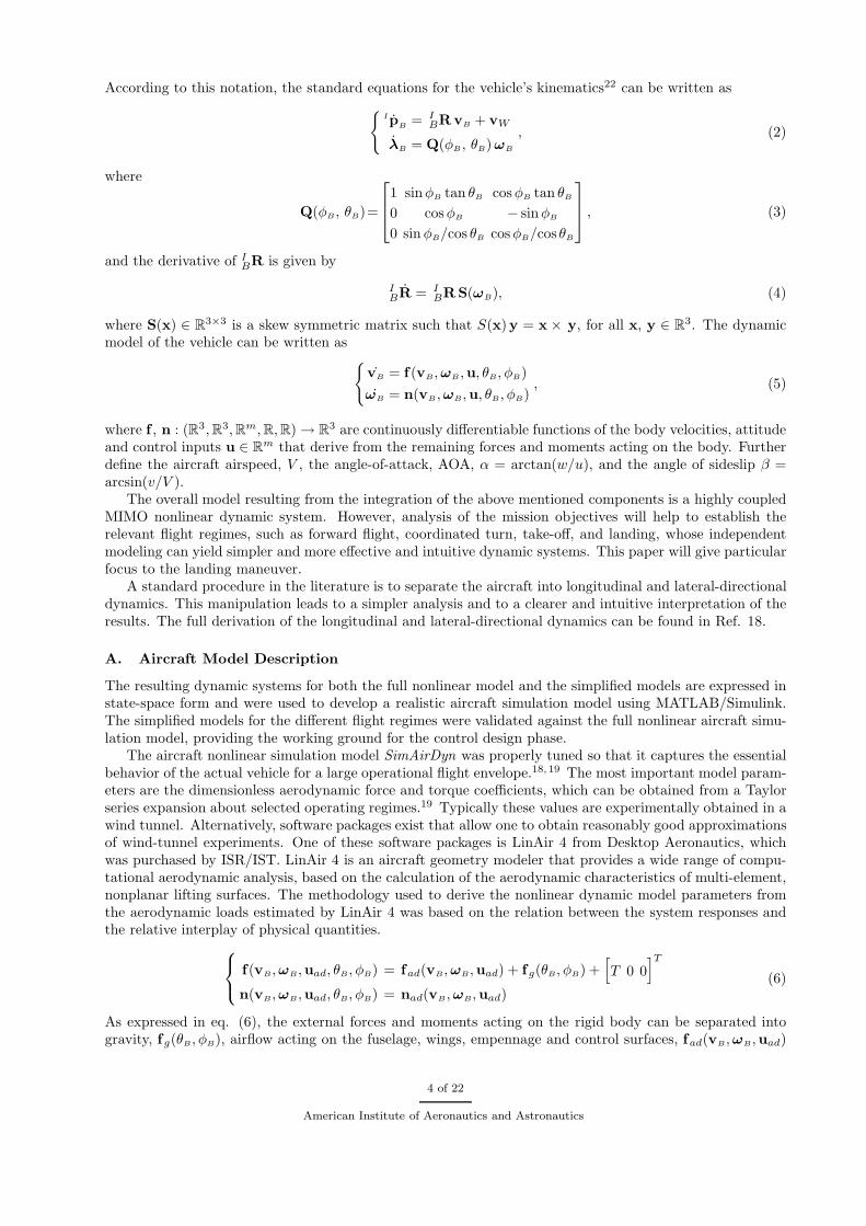
For the nonlinear simulation model to match the actual aircraft actuators, rate limitations and saturationwere included. The rate limitation is modeled using the system depicted in Figure 2, where αa = 50 rad/s.The rate limit is αak = 7 rad/s for the control surfaces, and αak = 10 N/s for the thrust. The saturationof actuators was set to ±30 degrees for the surfaces and 110 N for the thrust generated by the propeller. Inthe figure, ur is the reference control input and u is the corresponding rate limited control signal applied tothe aircraft.

k

aaur

-

u

Figure 2. Rate limitation system for the actuators

B. Model Analysis

A standard approach followed in aircraft stability analysis assumes that the coupling between lateral-directional and longitudinal modes can be neglected, and that, for a given flight condition, the airplanemotion can be described by two independent lower-order linear systems.

1. Longitudinal Dynamics

Let xlong(t) = [u(t)/V0 α(t) q(t) θB(t)]T

denote the vector of incremental longitudinal state variables about

equilibrium trajectories, where V0 is the steady-state airspeed given by V0 =√

u20 + v2

0 + w20 , α the AOA, q

the pitch angle rate, and θB the pitch angle that describes the rotation of the airplane about the y-axis ofthe body frame. After linearizing the longitudinal dynamics, one obtains

xlong(t) = Alongxlong(t) + BlongδLong(t) (7)

where δLong = [T, δaC, δf , δe]

T is the vector of incremental longitudinal control inputs. T is the thrustgenerated by the propeller, δaC

is referred to as the common-mode of the ailerons, δf is the flaps deflectionangle and δe is the elevator deflection angle. The common-mode of the ailerons is defined as

δaC=δaL

+ δaR

2(8)

where δaLand δaR

are the left and right ailerons incremental deflection angles, respectively.The eigenvalues of Along typically form two pairs of complex conjugate poles and define two natural

modes for the system. Using the standard notation, these can be described by

λ = −ωnξ ± ωn

√

1 − ξ2

5 of 22


where ωn is the natural frequency of the mode and ξ the damping coefficient. The fastest mode affectsmostly the AOA and the pitch angle of the vehicle, with major impact on the states α, θB and q. Whenexcited, this mode takes only a few seconds to reach steady-state and depends mainly on the relative locationof the center of mass (CM) of the airplane and its neutral point (NP). The NP is the virtual location wherethe CM should be for the aircraft to have neutral longitudinal stability. It can be shown that if the NP islocated aft of the CM, then the airplane is longitudinally stable.18

The slowest mode, commonly referred to as phugoid, affects mainly the normalized longitudinal velocityu/V0, and the pitch angle θB. The AOA and the pitch rate remain almost unchanged. Since q is nearzero, this mode is usually called the slow longitudinal mode. This mode can be physically interpreted as anoscillation on the altitude of the aircraft with cyclic transfers between kinetic energy and potential energy.

For the aircraft illustrated in Figure 1, the linearized model obtained when the vehicle describes a straightline path, at a speed of 30 m/s, has the fastest mode with frequency 14.31 rad/s and damping coefficientof 0.95. The phugoid mode is characterized by a frequency of 0.32 rad/s, which corresponds to a period ofabout 19.6 s, and a damping coefficient of 0.1.

2. Lateral-Directional Dynamics

For the lateral-directional dynamics, the incremental state vector can be defined as

xld(t) = [β(t) p(t) φB(t) r(t)]T

(9)

where β is the angle of sideslip, φB, the roll angle, p = φB and r = ψB, the roll and yaw rates, respectively.For the sake of completeness, we can write

xld(t) = Aldxld(t) + Bldδld(t) (10)

where δld = [δaD, δr]

T is the vector of incremental longitudinal control inputs, δaDis the differential-mode

of the ailerons given by eq. 11, and δr is the rudder angle.

δaD=δaL

− δaR

2(11)

The lateral-directional dynamics is known to have one pair of complex conjugate poles and two poles onthe real axis. The fastest of the real poles can be related to the roll angle, φB, affecting mainly this stateand its derivative, p. Therefore, this mode describes a pure roll maneuver, since all other states remainunchanged. The other real pole is related to the spiral mode. In some airplanes, this mode is unstableleading the aircraft to naturally enter into a decreasing radius spiral trajectory.

The remaining pair of complex conjugate poles is associated with the so-called Dutch-roll mode. For thismode, it can be shown that the sideslip and the yaw angles have a phase difference close to 180 degrees. Thisis reasonable from a physical point of view since, along an equilibrium trajectory, if the yaw angle suffers adisturbance, then it will also generate a sideslip angle disturbance with opposite sign, due to the definitionof angle β. In fact, this generates an oscillatory movement of the CM about a straight line defined by themean velocity of the airplane, together with a roll motion induced by the airflow asymmetry on the aircraftwings created by a nonzero sideslip angle.

Using the same trimming condition as before, a pure roll mode with a frequency of 205 rad/s wasidentified. The Dutch-roll mode was found with a frequency of 11.8 rad/s and a damping coefficient of 0.14and a slower unstable eigenvalue with frequency 0.023 rad/s was associated to the spiral mode.

C. Flaps

The flaps constitute a special type of actuators that are commonly used in manned airplanes during thelanding phase. They are control surfaces placed on the wings, usually near the fuselage, with objective ofextending the wings’ chord. This increases both the lift and the drag forces acting on the airplane, allowingfor lower speed flight trajectories. Although they are important on large aircrafts, they are not necessarilyemployed in smaller ones.

Since flaps are very slow control surfaces when compared to the rest of the aircraft actuators, they mustbe treated differently. In the present case study, they will be used in a stepwise manner, as a function of theaircraft’s height. This corresponds to the standard technique used in manned aircrafts.

6 of 22


III. Path-dependent Error Dynamic Model

The main objective of the present work is the design of a controller to steer the aircraft along the finalapproach phase which is associated with a smooth three-dimensional curve denoted by Γ. During this phase,the aircraft aligns itself with the runway and stabilizes about a constant sink rate and decreasing velocitymaneuver, called glideslope, until the flare maneuver brings it to touchdown. In this section, we present thetransformation applied to the aircraft dynamics (5) to obtain an error dynamic model, which will then beused to design controllers both for the glideslope and flare maneuvers.

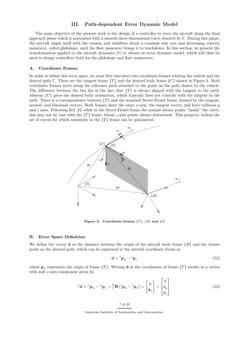
A. Coordinate Frames

In order to define this error space, we must first introduce two coordinate frames relating the vehicle and thedesired path Γ. These are the tangent frame {T } and the desired body frame {C} shown in Figure 3. Bothcoordinate frames move along the reference path attached to the point on the path closest to the vehicle.The difference between the two lies in the fact that {T } is always aligned with the tangent to the path,whereas {C} gives the desired body orientation, which typically does not coincide with the tangent to thepath. There is a correspondence between {T } and the standard Serret-Frenet frame, formed by the tangent,normal, and binormal vectors. Both frames share the same x-axis, the tangent vector, and have collinear yand z axes. Following Ref. 23, while in the Serret-Frenet frame the normal always points “inside” the curve,this may not be case with the {T } frame, whose z-axis points always downwards. This property widens theset of curves for which continuity in the {T } frame can be guaranteed.

Figure 3. Coordinate frames {T}, {B} and {I}

B. Error Space Definition

We define the vector d as the distance between the origin of the aircraft body frame {B} and the closestpoint on the desired path, which can be expressed in the inertial coordinate frame as

d = IpB− Ip

T(12)

where pT

represents the origin of frame {T }. Writing d in the coordinates of frame {T } results in a vectorwith null x-axis component given by

T d = TpB− T p

T= T

I R (IpB− Ip

T) =

[

0

dT

]

=

0

dy

dz

. (13)

7 of 22


The linear and angular velocities of frame {T } relative to the inertial frame, expressed in {T }, are given

by T (IvT) = vT =[

VT 0 0]T

and T (IωT ) = ωT = VT

[

τ 0 k]T

, respectively, where VT is the linear speed,

and κ and τ are trajectory parameters defined in Ref. 9. Using these expressions and taking the timederivative of vector dT one obtains

[

0

dT

]

= ˙TI R (Ip

B− Ip

T) + T

I R(

˙IpB− ˙Ip

T

)

= −S(ωT )

[

0

dT

]

+ TI RI

BRvB − TI RI

TRvT

= −S

VT

τ

0

k

[

0

dT

]

+ TBRvB −

VT

0

0

= −VT

−k dy

−τ dz

τ dy

+ T

BRvB −

VT

0

0

, (14)

and consequently

VT =1

1 − k dy

[

1 0 0]

TBRvB. (15)

In order to ensure that the vehicle not only follows a predefined curve Γ but also tracks a given velocityprofile, as is mandatory for the kind of maneuvers considered in the present paper, extra reference signalsare needed. For that purpose, we consider the reference tangent speed Vr, which defines references for boththe linear and angular tangent velocities given by

vr = Vr

1

0

0

=Vr

VT

vT ωr =Vr

VT

ωT , . (16)

respectively. The desired orientation can be represented by the Z-Y-X Euler angles λC = [φC θC ψC ]T,

θC ∈ ]−π/2, π/2[ , φC , ψC ∈ R. Given the definitions of {T }, {C}, and references vr and ωr, we introducethe following error state vector

xe =

ve

ωe

dT

λe

=

vB − BT Rvr

ωB − BT Rωr

[

0 1 0

0 0 1

]

TI R (Ip

B− p

C)

λB − λC

, (17)

where the states ve and ωe are used for velocity profile tracking, while the distance dT allows for path-following. Finally, the error λe is used to obtain aircraft attitude convergence. ¿From eq. (17), it isstraightforward to observe that the aircraft follows the path (dT = 0) with the linear speed ‖vB‖ = VT = VT

and orientation λB = λC if and only if xe = 0.Under these constraints, the error dynamics24 can be written as

ve = vB + S(ωe)BT Rvr +

(

1 −VT

Vr

)

BT RS(ωr)vr

ωe = ωB + S(ωe)BT Rωr

dT =VT τ

[

0 1

−1 0

]

dT +

[

0 1 0

0 0 1

]

TBRve

λe = Q(φB , θB)ωB − sign(κ)VT

√

κ2 + τ2[0 0 1]T

. (18)

The set of allowable paths is now restricted to the set of trimming paths. Similarly, the reference speed,Vr, and the motion of {C} are constrained to correspond to trimming trajectories consistent with the chosenpath. A trimming path corresponds to a curve that the aircraft can follow while satisfying the trimmingcondition, which is equivalent to having vB = 0, ωB = 0, and u = 0 in (5). It is well known that, for avehicle with dynamics described by (5) and assuming constant gravitational acceleration, the set of trimmingtrajectories comprises all z-aligned helices and straight-line trajectories. In the application presented here,

8 of 22


the aircraft is expected to track trajectories in the vertical plane with no sideslip, which correspond to theglideslope and flare maneuvers, reducing the allowed trimming paths to vertical plane straight lines. Underthese assumptions, the desired flight envelope can be parameterized by the vector ξ = (Vr , θT , θC, δf ), whereθT is the well known flight path angle γ, θC the aircraft pitch angle, and δf the deflection of the flaps.

To accomplish the tracking objectives during the sensitive landing maneuvers we define an output vectorye that corresponds to a combination of error components expressed on the body coordinate system, to bedriven to zero at steady-state by means of integral action. To summarize the foregoing considerations, theerror dynamic system for an aircraft can be written as

P(ξ) :=

{

xe = fe(xe,u, ξ)

y = g(xe, ξ), (19)

where the output to be integrated satisfies, for allowed values of ξ = ξ0, g(0, ξ0) = 0. Recalling that ξ isa constant parameter vector, the linearization of P(ξ) about (xe = 0, u = uξ) results in a time-invariantsystem of the form

Pl(ξ) =

{

δxe = Ae(ξ)δxe +Be(ξ)δu

δye = Ce(ξ)δxe

, (20)

where Ae(ξ) =∂fe

∂xe(0,uξ, ξ), Be(ξ) =

∂fe

∂u(0,uξ, ξ), and Ce(ξ) =

∂g

∂xe(0, ξ).

IV. Controller Synthesis

Aircraft dynamic models are complex nonlinear systems that are in general functions of the dynamicpressure and angles of attack and side-slip. Hence, it is inadequate, for control purposes, to representthem by LTI models. Linear Parameter Varying models embody nowadays a compromise between theglobal accuracy of nonlinear models and the straightforward controller synthesis techniques available forLTI representations. These parameter dependent systems arise naturally while modeling physical systems,where the corresponding state space description depends on a set of parameters. In the present work, apiecewise affine dependence on the parameters will be considered to accurately model the error dynamicsover a wide flight-envelope. The identification of LPV models, given the model structure and order, isaddressed determining the number of local models, the set of operating points, and the set of variables thatcan be used to form the scheduling vector.

In the approach pursued in this paper, results presented in Refs. 25, 26 were used to develop the LMIbased controller synthesis algorithm for affine parameter dependent systems. Much of the work in this areais well rooted in the theory of LMIs, which provide a powerful formulation framework as well as a versatiledesign technique for a wide variety of linear control problems. Since solving LMIs is a convex optimizationproblem for which efficient numerical solvers are now available, an LMI based formulation can be seen as apractical solution for many control problems.

A. Design Specifications

The linear controllers for the glideslope and flare maneuvers are required to meet the following designspecifications:

Zero Steady State Error. Achieve zero steady state values for the distance to the reference path, thelinear velocity error, and the roll angle.

Bandwidth Requirements. The input-output command response bandwidth for the path following errorchannels should be on the order of 0.1 rad/s; the control loop bandwidth for the deflection surfaceschannels should not exceed 5 rad/s, to ensure that the actuators would not be driven beyond theirnormal actuation bandwidth.

Closed Loop Damping and Stability Margins. The closed loop eigenvalues should have a damping ratioof a least 0.7 and a magnitude of at least 0.1 rad/s.

Glideslope. In this phase of the maneuver it will be required to achieve zero steady state deflection ofthe common mode of the ailerons δaC

= 0.

9 of 22


Flare. In this phase of the landing maneuver, the aircraft should achieve zero steady state error inresponse to pitch angle commands.

To satisfy the design requirements we introduce the following integral error for the glideslope maneuver

x1

x2

x3

=

∫

φedt∫ (

ve +BT

R [0 dT

T]T)

dt∫

δaCdt

(21)

where φe = φC −φB. For the flare maneuver, to satisfy the tracking requirements on the aircraft pitch anglewe remove the state x3 and introduce a new integral state x4, defined as

x4 =

∫

θedt. (22)

where θe = θC −θB. Two different control objectives have been introduced. The switching between states x3

and x4, requires the use of different controllers, one for each case. Notice that, when the state x4 is selected,the airspeed and pitch references profiles should agree, in order to keep the aircraft control surfaces awayfrom saturation during the controller switching. Furthermore, the reference pitch angle close the touchdowndepends on the aircraft weight. When the mass increases, the reference pitch angle should also increase, toproduce the required lift force without recruiting the actuators.

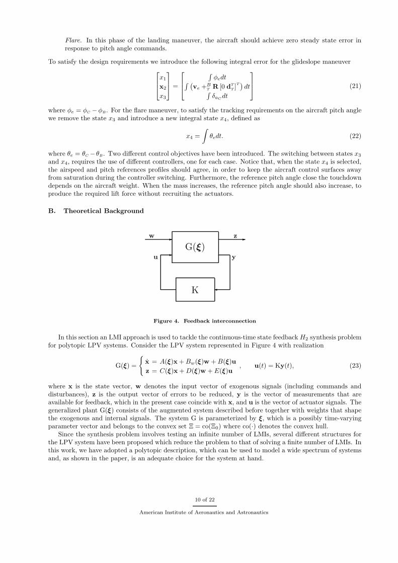
B. Theoretical Background

K

-

G(ξ)

�

--w z

yu

Figure 4. Feedback interconnection

In this section an LMI approach is used to tackle the continuous-time state feedbackH2 synthesis problemfor polytopic LPV systems. Consider the LPV system represented in Figure 4 with realization

G(ξ) =

{

x = A(ξ)x +Bw(ξ)w +B(ξ)u

z = C(ξ)x +D(ξ)w + E(ξ)u, u(t) = Ky(t), (23)

where x is the state vector, w denotes the input vector of exogenous signals (including commands anddisturbances), z is the output vector of errors to be reduced, y is the vector of measurements that areavailable for feedback, which in the present case coincide with x, and u is the vector of actuator signals. Thegeneralized plant G(ξ) consists of the augmented system described before together with weights that shapethe exogenous and internal signals. The system G is parameterized by ξ, which is a possibly time-varyingparameter vector and belongs to the convex set Ξ = co(Ξ0) where co(·) denotes the convex hull.

Since the synthesis problem involves testing an infinite number of LMIs, several different structures forthe LPV system have been proposed which reduce the problem to that of solving a finite number of LMIs. Inthis work, we have adopted a polytopic description, which can be used to model a wide spectrum of systemsand, as shown in the paper, is an adequate choice for the system at hand.

10 of 22


Definition IV.1 (Polytopic LPV system). The system (23) is said to be a polytopic LPV system with affineparameter dependence if the system matrix

S(ξ) =

[

A(ξ) Bw(ξ) B(ξ)

C(ξ) D(ξ) E(ξ)

]

(24)

verifies S(ξ) = S(0) +∑np

j=1 S(j)ξj , for all ξ = [ξ1 . . . ξnp

]T ∈ Ξ, and the parameter set takes the formΞ = co(Ξ0), where

Ξ0 = {ξ ∈ Rnp | ξi ∈ {ξ

i, ξi}, ξi

≤ ξi, i = 1, . . . , np} .

We are interested in finding a solution to the continuous-time state feedback H2 synthesis problem.Consider the static state feedback law given by u = Kx and let Tzw denote the closed-loop operator from w

to z. Then, the H2 synthesis problem can be described as that of finding a control matrix K that stabilizesthe closed-loop system and minimizes the H2 norm ‖Tzw‖2. Note that matrix D(ξ) = 0 in order to guaranteethat ‖Tzw‖2 is finite for every internally stabilizing and strictly proper controller. The technique used forcontroller design relies on results available in Refs. 27,28, after being rewritten for the case of polytopic LPVsystems. In the following, tr(L) denotes the trace of matrix L.

Result IV.1. A static state feedback controller guarantees the ζ upper-bound for the continuous-time H2

norm of the closed-loop operator Tzw(ξ) for all ξ ∈ Ξ, that is,

‖Tzw(ξ)‖2 < ζ, ∀ξ ∈ Ξ (25)

if there are real matrices X = XT > 0, Y > 0, and W such that[

A(ξ)X +X A(ξ)T +B(ξ)W +WT B(ξ)T Bw(ξ)

Bw(ξ)T −I

]

< 0 (26a)

[

Y C(ξ)X + E(ξ)W

X C(ξ)T +WT E(ξ)T X

]

> 0 (26b)

tr (Y ) < ζ2 . (26c)

for all ξ ∈ Ξ0. The respective controller gain matrix is given by K = W X−1.

Additional closed-loop regional eigenvalues placement specifications for each plant G(ξ) in the polytopicregion can also be converted into design constraints resorting to the concept of LMI regions in the complexplane introduced in Ref. 29. These constitute a generalization of the well known α-stability region presentednext.

Result IV.2. The closed-loop system with realization (23) has all the eigenvalues in the semi-plane λ ∈ C :Re(λ) < −α for all ξ ∈ Ξ if matrices X = XT > 0 and W exist such that the closed-loop Lyapunov inequality

A(ξ)X +X A(ξ)T +B(ξ)W +WT B(ξ)T + 2αI < 0 (27)

is satisfied for all ξ ∈ Ξ0.

This well known result can be generalized as follows. Let L = [lij ] and M = [mij ] be real symmetricmatrices. An LMI region Rlmi is defined as an open domain in the complex plane that satisfies

Rlmi = {z ∈ C : lij +mijz +mjiz < 0; i, j = 1, ..., n} . (28)

This description can represent a large number of regions which are symmetric with respect to the real axis,such as conic sectors, half-planes, etc. Using the concept of LMI regions, Result IV.2 admits the followinggeneralization29

Result IV.3. The closed-loop system with realization (23) has all the eigenvalues in the region Rcl defined

by (28) for all ξ ∈ Ξ if a real symmetric matrix X > 0 exists such that the generalized Lyapunov inequality

lijX +mij(A(ξ)X +B(ξ)W ) +mji(X A(ξ)T +WT B(ξ)T ) < 0; i, j = 1, ..., n (29)

is satisfied.

11 of 22


θreg

Im(z)

Re(z)−αreg

Figure 5. A typical closed-loop generalized stability region

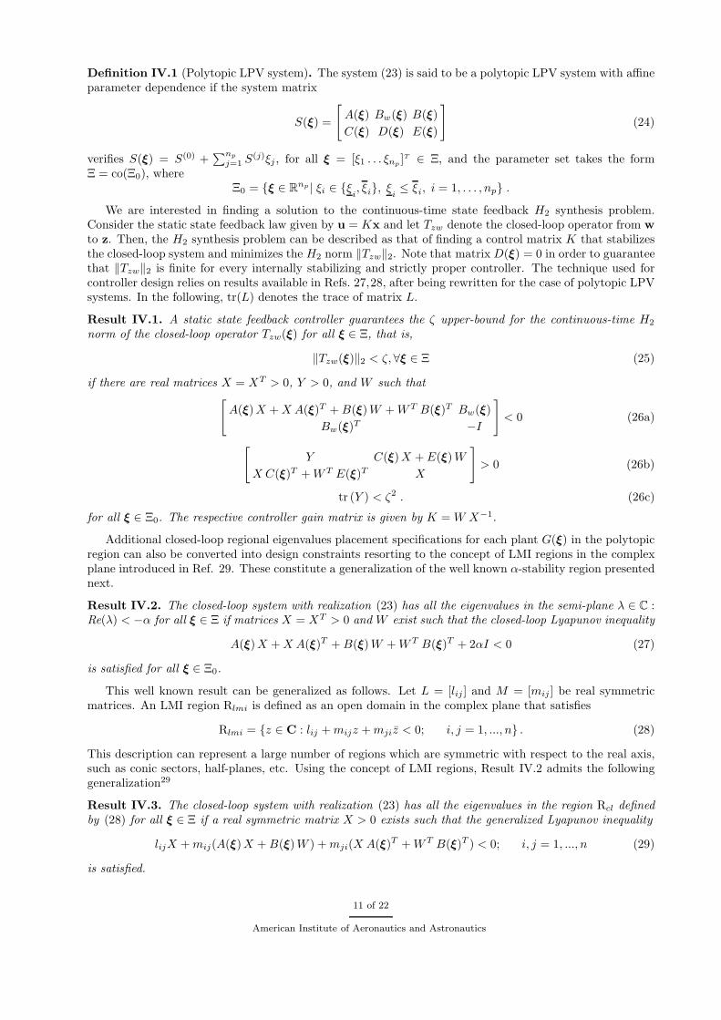
In the present design case, the closed-loop eigenvalues are required to lie in the region depicted in Figure 5.Simple computations show that in this case (29) degenerates into

sin(θreg)(∆(ξ) + ∆(ξ)T ) cos(θreg)(∆(ξ)T − ∆(ξ)) 0

cos(θreg)(∆(ξ) − ∆(ξ)T ) sin(θreg)(∆(ξ) + ∆(ξ)T ) 0

0 0 ∆(ξ) + ∆(ξ)T + 2αregX

< 0, (30)

where ∆(ξ) = A(ξ)X + B(ξ)W and parameters αreg and θreg were set to αcl = 0.1, and θcl = 45o,respectively, so as to meet the desired closed-loop performance specifications.

The optimal solution for the continuous-time H2 control problem is approximated through the minimiza-tion of ζ subject to the LMIs presented in (26) and (30).

C. Computation of the LPV System Matrices

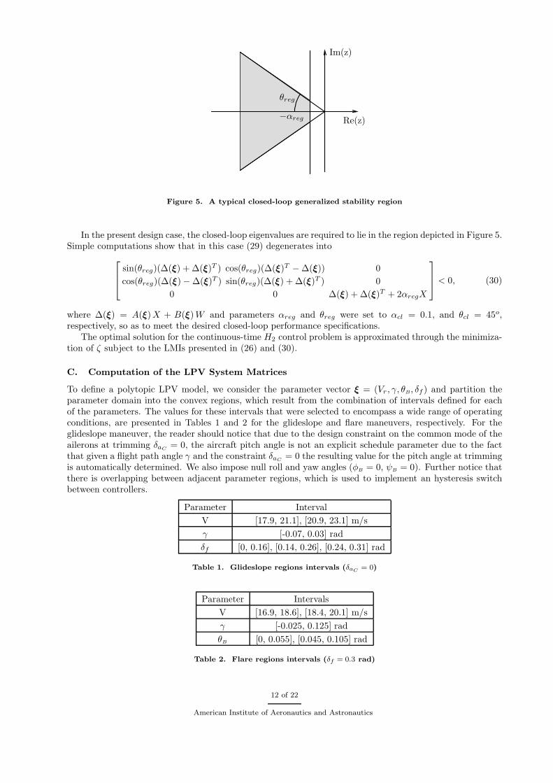
To define a polytopic LPV model, we consider the parameter vector ξ = (Vr , γ, θB, δf ) and partition theparameter domain into the convex regions, which result from the combination of intervals defined for eachof the parameters. The values for these intervals that were selected to encompass a wide range of operatingconditions, are presented in Tables 1 and 2 for the glideslope and flare maneuvers, respectively. For theglideslope maneuver, the reader should notice that due to the design constraint on the common mode of theailerons at trimming δaC

= 0, the aircraft pitch angle is not an explicit schedule parameter due to the factthat given a flight path angle γ and the constraint δaC

= 0 the resulting value for the pitch angle at trimmingis automatically determined. We also impose null roll and yaw angles (φB = 0, ψB = 0). Further notice thatthere is overlapping between adjacent parameter regions, which is used to implement an hysteresis switchbetween controllers.

Parameter Interval

V [17.9, 21.1], [20.9, 23.1] m/s

γ [-0.07, 0.03] rad

δf [0, 0.16], [0.14, 0.26], [0.24, 0.31] rad

Table 1. Glideslope regions intervals (δaC= 0)

Parameter Intervals

V [16.9, 18.6], [18.4, 20.1] m/s

γ [-0.025, 0.125] rad

θB [0, 0.055], [0.045, 0.105] rad

Table 2. Flare regions intervals (δf = 0.3 rad)

12 of 22


Within each region, the state space matrices of the continuous-time system (20) were approximated byan affine function of ξ using Least Squares Fitting applied to a relatively dense grid of evaluated operatingpoints. Then, the resulting system was evaluated at the vertices of each region, producing the finite set ofstate space matrices needed for control system design.

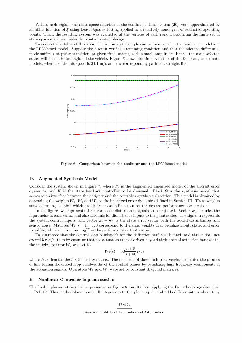
To access the validity of this approach, we present a simple comparison between the nonlinear model andthe LPV-based model. Suppose the aircraft verifies a trimming condition and that the ailerons differentialmode suffers a stepwise transition, at given time instant, with a small amplitude. Hence, the main affectedstates will be the Euler angles of the vehicle. Figure 6 shows the time evolution of the Euler angles for bothmodels, when the aircraft speed is 21.1 m/s and the corresponding path is a straight line.

0 1 2 3 4 5 6 7 8 9 10−0.01

−0.005

0

0.005

0.01

0.015

0.02

Time [s]

Eul

er a

ngle

s [r

ad]

φ − NL Modelφ − LPV Modelθ − NL Modelθ − LPV Modelψ − NL Modelψ − LPV Model

Figure 6. Comparison between the nonlinear and the LPV-based models

D. Augmented Synthesis Model

Consider the system shown in Figure 7, where Pe is the augmented linearized model of the aircraft errordynamics, and K is the state feedback controller to be designed. Block G is the synthesis model thatserves as an interface between the designer and the controller synthesis algorithm. This model is obtained byappending the weights W1, W2 and W3 to the linearized error dynamics defined in Section III. These weightsserve as tuning “knobs” which the designer can adjust to meet the desired performance specifications.

In the figure, w1 represents the error space disturbance signals to be rejected. Vector w2 includes theinput noise to each sensor and also accounts for disturbance inputs to the plant states. The signal u representsthe system control inputs, and vector xe + w1 is the state error vector with the added disturbances andsensor noise. Matrices Wi, i = 1, . . . , 3 correspond to dynamic weights that penalize input, state, and errorvariables, while z = [z1 z2 z3]

T is the performance output vector.To guarantee that the control loop bandwidth for the deflection surfaces channels and thrust does not

exceed 5 rad/s, thereby ensuring that the actuators are not driven beyond their normal actuation bandwidth,the matrix operator W2 was set to

W2(s) = 50s+ 5

s+ 50I5×5

where I5×5 denotes the 5 × 5 identity matrix. The inclusion of these high-pass weights expedites the processof fine tuning the closed-loop bandwidths of the control planes by penalizing high frequency components ofthe actuation signals. Operators W1 and W3 were set to constant diagonal matrices.

E. Nonlinear Controller implementation

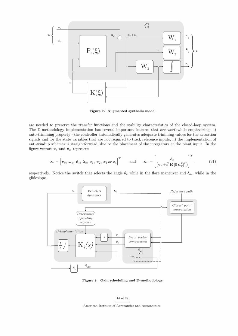
The final implementation scheme, presented in Figure 8, results from applying the D-methodology describedin Ref. 17. This methodology moves all integrators to the plant input, and adds differentiators where they

13 of 22


u

w1

K( )x

Pe( )x

W1

W2

W3

u

w2

xe z1

z2

z3

x +e 1w

G

z

w

Figure 7. Augmented synthesis model

are needed to preserve the transfer functions and the stability characteristics of the closed-loop system.The D-methodology implementation has several important features that are worthwhile emphasizing: i)auto-trimming property - the controller automatically generates adequate trimming values for the actuationsignals and for the state variables that are not required to track reference inputs; ii) the implementation ofanti-windup schemes is straightforward, due to the placement of the integrators at the plant input. In thefigure vectors xe and xD represent

xe =[

ve, ωe, dt, λe, x1, x2, x3 or x4

]T

and xD =

[

φe(

ve +BT

R [0 dT

T]T)

]T

, (31)

respectively. Notice the switch that selects the angle θe while in the flare maneuver and δaCwhile in the

glideslope.

Vehicle`sdynamics

u xB

Error vectorcomputation

Determinesoperatingregion i

Ki(s)

D-Implementation

Reference path

Closest pointcomputation

1s

qe

s

Sa

dac

xe

xD

Figure 8. Gain scheduling and D-methodology

14 of 22


F. Landing Maneuvers

Next, the maneuvers for both landing phases are presented. We assume the runway approaching maneuverhas been completed which means that the aircraft is already aligned with the runway, at a predefined height,and ready for the glideslope to start.

1. Glideslope Maneuver

During the glideslope, the aircraft should have a constant flight path angle, γgs, corresponding to a straight-line descending path until the start of the flare maneuver. Also, the airspeed should decrease along the pathand the roll angle should be close to zero. It should be noticed that the aircraft AOA is not imposed. In fact,as the common mode of the ailerons is automatically driven to zero, the AOA will depend on the airspeed,on the flaps deflection, and on the load of the aircraft.

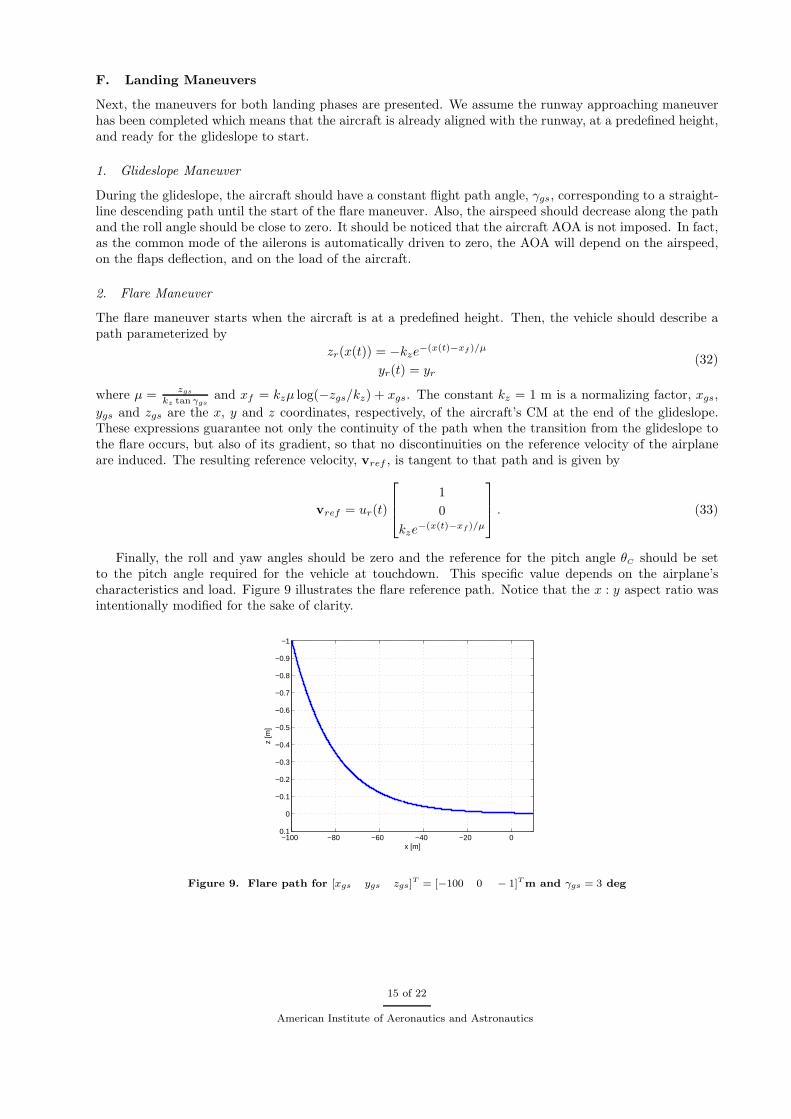
2. Flare Maneuver

The flare maneuver starts when the aircraft is at a predefined height. Then, the vehicle should describe apath parameterized by

zr(x(t)) = −kze−(x(t)−xf)/µ

yr(t) = yr

(32)

where µ =zgs

kz tan γgsand xf = kzµ log(−zgs/kz) + xgs. The constant kz = 1 m is a normalizing factor, xgs,

ygs and zgs are the x, y and z coordinates, respectively, of the aircraft’s CM at the end of the glideslope.These expressions guarantee not only the continuity of the path when the transition from the glideslope tothe flare occurs, but also of its gradient, so that no discontinuities on the reference velocity of the airplaneare induced. The resulting reference velocity, vref , is tangent to that path and is given by

vref = ur(t)

1

0

kze−(x(t)−xf)/µ

. (33)

Finally, the roll and yaw angles should be zero and the reference for the pitch angle θC should be setto the pitch angle required for the vehicle at touchdown. This specific value depends on the airplane’scharacteristics and load. Figure 9 illustrates the flare reference path. Notice that the x : y aspect ratio wasintentionally modified for the sake of clarity.

−100 −80 −60 −40 −20 0

−1

−0.9

−0.8

−0.7

−0.6

−0.5

−0.4

−0.3

−0.2

−0.1

0

0.1

x [m]

z [m

]

Figure 9. Flare path for [xgs ygs zgs]T = [−100 0 − 1]T m and γgs = 3 deg

15 of 22


V. Simulation Results

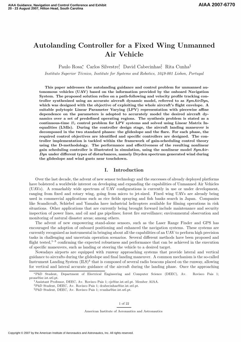
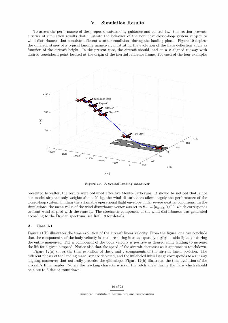
To assess the performance of the proposed autolanding guidance and control law, this section presentsa series of simulation results that illustrate the behavior of the nonlinear closed-loop system subject towind disturbances that simulate different weather conditions during the landing phase. Figure 10 depictsthe different stages of a typical landing maneuver, illustrating the evolution of the flaps deflection angle asfunction of the aircraft height. In the present case, the aircraft should land on a x aligned runway withdesired touchdown point located at the origin of the inertial reference frame. For each of the four examples

−3000−2500

−2000−1500

−1000−500

0

−150

−100

−50

0

50

100

150

−150

−100

−50

0

y [m]

Flare Start

x [m]

Flaps 17º

Flaps 11º

Flaps 6º

Glideslope Start

z [m

]

Figure 10. A typical landing maneuver

presented hereafter, the results were obtained after five Monte-Carlo runs. It should be noticed that, sinceour model-airplane only weights about 20 kg, the wind disturbances affect largely the performance of theclosed-loop system, limiting the attainable operational flight envelope under severe weather conditions. In thesimulations, the mean value of the wind disturbance vector was set to vW = [uwind, 0, 0]

T, which corresponds

to front wind aligned with the runway. The stochastic component of the wind disturbances was generatedaccording to the Dryden spectrum, see Ref. 19 for details.

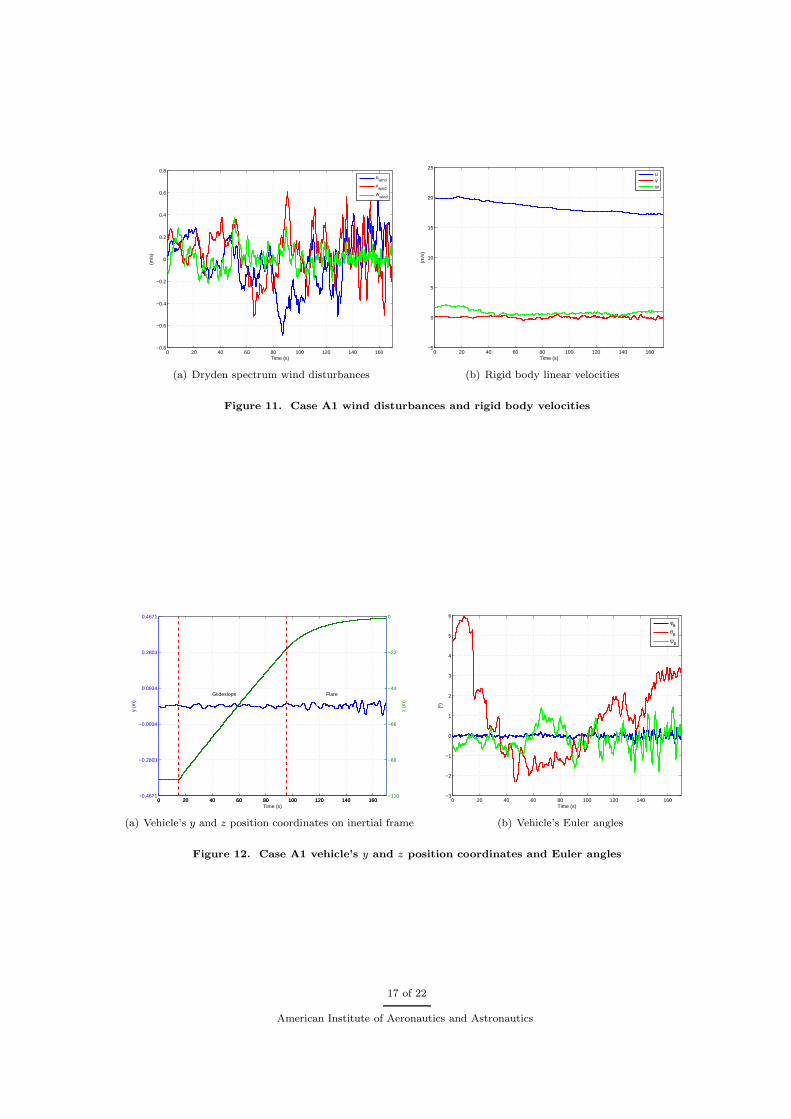
A. Case A1

Figure 11(b) illustrates the time evolution of the aircraft linear velocity. From the figure, one can concludethat the component v of the body velocity is small, resulting in an adequately negligible sideslip angle duringthe entire maneuver. The w component of the body velocity is positive as desired while landing to increasethe lift for a given airspeed. Notice also that the speed of the aircraft decreases as it approaches touchdown.

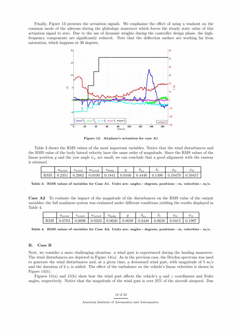
Figure 12(a) shows the time evolution of the y and z components of the aircraft linear position. Thedifferent phases of the landing maneuver are depicted, and the unlabeled initial stage corresponds to a runwayaligning maneuver that naturally precedes the glideslope. Figure 12(b) illustrates the time evolution of theaircraft’s Euler angles. Notice the tracking characteristics of the pitch angle during the flare which shouldbe close to 3 deg at touchdown.

16 of 22


0 20 40 60 80 100 120 140 160−0.8

−0.6

−0.4

−0.2

0

0.2

0.4

0.6

0.8

Time (s)

(m/s

)

u

wind

vwind

wwind

(a) Dryden spectrum wind disturbances

0 20 40 60 80 100 120 140 160−5

0

5

10

15

20

25

Time (s)

(m/s

)

uvw

(b) Rigid body linear velocities

Figure 11. Case A1 wind disturbances and rigid body velocities

0 20 40 60 80 100 120 140 160−0.4671

−0.2803

−0.0934

0.0934

0.2803

0.4671

y (m

)

Time (s)

Glideslope Flare

0 20 40 60 80 100 120 140 160−110

−88

−66

−44

−22

0

z (m

)

(a) Vehicle’s y and z position coordinates on inertial frame

0 20 40 60 80 100 120 140 160−3

−2

−1

0

1

2

3

4

5

6

Time (s)

(º)

φ

B

θB

ψB

(b) Vehicle’s Euler angles

Figure 12. Case A1 vehicle’s y and z position coordinates and Euler angles

17 of 22


Finally, Figure 13 presents the actuation signals. We emphasize the effect of using a washout on thecommon mode of the ailerons during the glideslope maneuver which forces the steady state value of thisactuation signal to zero. Due to the use of dynamic weights during the controller design phase, the high-frequency components are significantly reduced. Note that the deflection surface are working far fromsaturation, which happens at 30 degrees.

0 20 40 60 80 100 120 140 160−10

−5

0

5

10

15

20

(º)

δa

c

δa

dδ

eδ

rδ

f

0 20 40 60 80 100 120 140 160−30

−20

−10

0

10

20

30

40

50

60

Time (s)

T (

N)

T

Figure 13. Airplane’s actuation for case A1

Table 3 shows the RMS values of the most important variables. Notice that the wind disturbances andthe RMS value of the body lateral velocity have the same order of magnitude. Since the RMS values of thelinear position y and the yaw angle ψB are small, we can conclude that a good alignment with the runwayis attained.

uwind vwind wwind vbody y δadδr φB ψB

RMS 0.2351 0.2082 0.0100 0.1841 0.0106 0.4446 0.1498 0.10479 0.59457

Table 3. RMS values of variables for Case A1. Units are: angles - degrees, positions - m, velocities - m/s.

Case A2 To evaluate the impact of the magnitude of the disturbances on the RMS value of the outputvariables, the full nonlinear system was evaluated under different conditions yielding the results displayed inTable 4.

uwind vwind wwind vbody y δadδr φB ψB

RMS 0.0783 0.0696 0.0333 0.0620 0.0039 0.3448 0.0620 0.0415 0.1997

Table 4. RMS values of variables for Case A2. Units are: angles - degrees, positions - m, velocities - m/s.

B. Case B

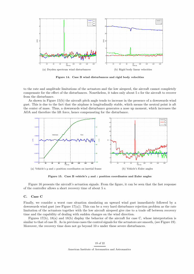
Next, we consider a more challenging situation: a wind gust is experienced during the landing maneuver.The wind disturbances are depicted in Figure 14(a). As in the previous case, the Dryden spectrum was usedto generate the wind disturbances and, at a given time, a downward wind gust, with magnitude of 5 m/sand the duration of 2 s, is added. The effect of the turbulence on the vehicle’s linear velocities is shown inFigure 14(b).

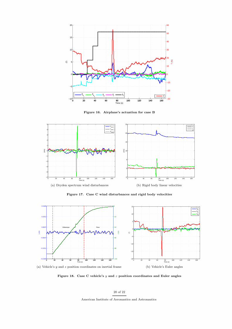
Figures 15(a) and 15(b) show how the wind gust affects the vehicle’s y and z coordinates and Eulerangles, respectively. Notice that the magnitude of the wind gust is over 25% of the aircraft airspeed. Due

18 of 22


0 20 40 60 80 100 120 140 160−1

0

1

2

3

4

5

Time (s)

(m/s

)

u

wind

vwind

wwind


0 20 40 60 80 100 120 140 160−5

0

5

10

15

20

25

Time (s)

(m/s

)

uvw


Figure 14. Case B wind disturbances and rigid body velocities

to the rate and amplitude limitations of the actuators and the low airspeed, the aircraft cannot completelycompensate for the effect of the disturbances. Nonetheless, it takes only about 5 s for the aircraft to recoverfrom the disturbance.

As shown in Figure 15(b) the aircraft pitch angle tends to increase in the presence of a downwards windgust. This is due to the fact that the airplane is longitudinally stable, which means the neutral point is aftthe center of mass. Thus, a downwards wind disturbance generates a nose up moment, which increases theAOA and therefore the lift force, hence compensating for the disturbance.

0 20 40 60 80 100 120 140 160−0.4121

−0.2472

−0.0824

0.0824

0.2472

0.4121

y (m

)

Time (s)

Glideslope Flare

0 20 40 60 80 100 120 140 160−110

−88

−66

−44

−22

0

z (m

)


0 20 40 60 80 100 120 140 160−4

−2

0

2

4

6

8

10

12

14

16

Time (s)

(º)

φ

B

θB

ψB


Figure 15. Case B vehicle’s y and z position coordinates and Euler angles

Figure 16 presents the aircraft’s actuation signals. From the figure, it can be seen that the fast responseof the controller allows a short recovery time of about 5 s.

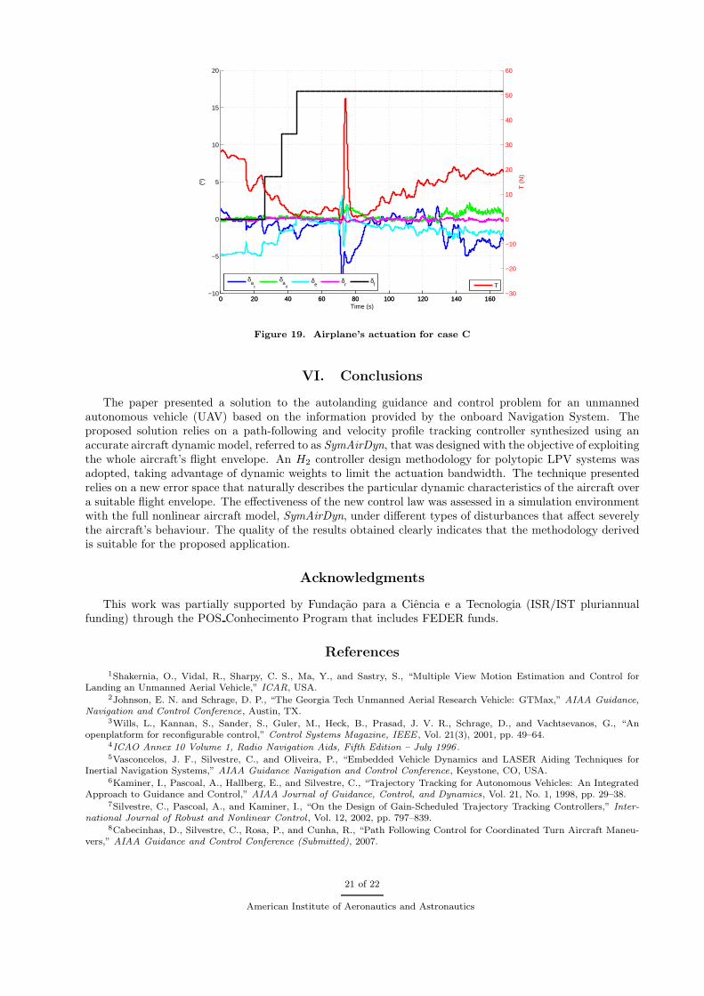
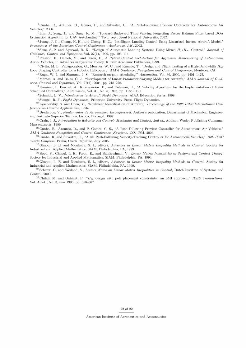
C. Case C

Finally, we consider a worst case situation simulating an upward wind gust immediately followed by adownwards wind gust (see Figure 17(a)). This can be a very hard disturbance rejection problem as the ratelimitation of the actuators together with the low aircraft airspeed give rise to a trade off between recoverytime and the capability of dealing with sudden changes on the wind direction.

Figures 17(b), 18(a) and 18(b) display the behavior of the aircraft for case C, whose interpretation issimilar to that of case B. As in previous cases the control signals for the actuators are smooth, (see Figure 19).Moreover, the recovery time does not go beyond 10 s under these severe disturbances.

19 of 22


0 20 40 60 80 100 120 140 160−10

−5

0

5

10

15

20

(º)

δa

c

δa

dδ

eδ

rδ

f

0 20 40 60 80 100 120 140 160−30

−20

−10

0

10

20

30

40

50

60

Time (s)

T (

N)

T

Figure 16. Airplane’s actuation for case B

0 20 40 60 80 100 120 140 160−5

−4

−3

−2

−1

0

1

2

3

4

5

Time (s)

(m/s

)

u

wind

vwind

wwind


0 20 40 60 80 100 120 140 160−5

0

5

10

15

20

25

Time (s)

(m/s

)

uvw


Figure 17. Case C wind disturbances and rigid body velocities

0 20 40 60 80 100 120 140 160−0.3185

−0.1911

−0.0637

0.0637

0.1911

0.3185

y (m

)

Time (s)

Glideslope Flare

0 20 40 60 80 100 120 140 160−110

−88

−66

−44

−22

0

z (m

)


0 20 40 60 80 100 120 140 160−20

−15

−10

−5

0

5

10

15

Time (s)

(º)

φ

B

θB

ψB


Figure 18. Case C vehicle’s y and z position coordinates and Euler angles

20 of 22


0 20 40 60 80 100 120 140 160−10

−5

0

5

10

15

20

(º)

δa

c

δa

dδ

eδ

rδ

f

0 20 40 60 80 100 120 140 160−30

−20

−10

0

10

20

30

40

50

60

Time (s)

T (

N)

T

Figure 19. Airplane’s actuation for case C

VI. Conclusions

The paper presented a solution to the autolanding guidance and control problem for an unmannedautonomous vehicle (UAV) based on the information provided by the onboard Navigation System. Theproposed solution relies on a path-following and velocity profile tracking controller synthesized using anaccurate aircraft dynamic model, referred to as SymAirDyn, that was designed with the objective of exploitingthe whole aircraft’s flight envelope. An H2 controller design methodology for polytopic LPV systems wasadopted, taking advantage of dynamic weights to limit the actuation bandwidth. The technique presentedrelies on a new error space that naturally describes the particular dynamic characteristics of the aircraft overa suitable flight envelope. The effectiveness of the new control law was assessed in a simulation environmentwith the full nonlinear aircraft model, SymAirDyn, under different types of disturbances that affect severelythe aircraft’s behaviour. The quality of the results obtained clearly indicates that the methodology derivedis suitable for the proposed application.

Acknowledgments

This work was partially supported by Fundacao para a Ciencia e a Tecnologia (ISR/IST pluriannualfunding) through the POS Conhecimento Program that includes FEDER funds.

References

1Shakernia, O., Vidal, R., Sharpy, C. S., Ma, Y., and Sastry, S., “Multiple View Motion Estimation and Control forLanding an Unmanned Aerial Vehicle,” ICAR, USA.

2Johnson, E. N. and Schrage, D. P., “The Georgia Tech Unmanned Aerial Research Vehicle: GTMax,” AIAA Guidance,Navigation and Control Conference, Austin, TX.

3Wills, L., Kannan, S., Sander, S., Guler, M., Heck, B., Prasad, J. V. R., Schrage, D., and Vachtsevanos, G., “Anopenplatform for reconfigurable control,” Control Systems Magazine, IEEE , Vol. 21(3), 2001, pp. 49–64.

4ICAO Annex 10 Volume 1, Radio Navigation Aids, Fifth Edition – July 1996 .5Vasconcelos, J. F., Silvestre, C., and Oliveira, P., “Embedded Vehicle Dynamics and LASER Aiding Techniques for

Inertial Navigation Systems,” AIAA Guidance Navigation and Control Conference, Keystone, CO, USA.6Kaminer, I., Pascoal, A., Hallberg, E., and Silvestre, C., “Trajectory Tracking for Autonomous Vehicles: An Integrated

Approach to Guidance and Control,” AIAA Journal of Guidance, Control, and Dynamics, Vol. 21, No. 1, 1998, pp. 29–38.7Silvestre, C., Pascoal, A., and Kaminer, I., “On the Design of Gain-Scheduled Trajectory Tracking Controllers,” Inter-

national Journal of Robust and Nonlinear Control , Vol. 12, 2002, pp. 797–839.8Cabecinhas, D., Silvestre, C., Rosa, P., and Cunha, R., “Path Following Control for Coordinated Turn Aircraft Maneu-

vers,” AIAA Guidance and Control Conference (Submitted), 2007.

21 of 22


9Cunha, R., Antunes, D., Gomes, P., and Silvestre, C., “A Path-Following Preview Controller for Autonomous AirVehicles,” 2006.

10Lim, J., Song, J., and Sung, K. M., “Forward-Backward Time Varying Forgetting Factor Kalman Filter based DOAEstimation Algorithm for UAV Autolanding,” Tech. rep., Seoul National University, 2002.

11Juang, J.-G., Chang, H.-H., and Cheng, K.-C., “Intelligent Landing Control Using Linearized Inverse Aircraft Model,”Proceedings of the American Control Conference - Anchorage, AK , 2002.

12Shue, S.-P. and Agarwal, R. K., “Design of Automatic Landing Systems Using Mixed H2/H∞ Control,” Journal ofGuidance, Control and Dynamics, Vol. 22(1), 1999, pp. 103–114.

13Frazzoli, E., Dahleh, M., and Feron, E., A Hybrid Control Architecture for Aggressive Maneuvering of AutonomousAerial Vehicles, In Advances in Systems Theory, Kluwer Academic Publishers, 1999.

14Civita, M. L., Papageorgiou, G., Messner, W. C., and Kanade, T., “Design and Flight Testing of a High-Bandwidth H∞

Loop Shaping Controller for a Robotic Helicopter,” AIAA Guidance, Navigation and Control Conference, Monterey, CA.15Rugh, W. J. and Shamma, J. S., “Research on gain scheduling,” Automatica, Vol. 36, 2000, pp. 1401–1425.16Marcos, A. and Balas, G. J., “Development of Linear-Parameter-Varying Models for Aircraft,” AIAA Journal of Guid-

ance, Control and Dynamics, Vol. 27(2), 2004, pp. 218–228.17Kaminer, I., Pascoal, A., Khargonekar, P., and Coleman, E., “A Velocity Algorithm for the Implementation of Gain-

Scheduled Controllers,” Automatica, Vol. 31, No. 8, 1995, pp. 1185–1191.18Schmidt, L. V., Introduction to Aircraft Flight Dynamics, AIAA Education Series, 1998.19Stengel, R. F., Flight Dynamics, Princeton University Press, Flight Dynamics.20Lyashevskiy, S. and Chen, Y., “Nonlinear Identification of Aircraft,” Proceedings of the 1996 IEEE lnternational Con-

ference on Control Applications, 1996.21Brederode, V., Fundamentos de Aerodinmica Incompressvel , Author’s publication, Department of Mechanical Engineer-

ing, Instituto Superior Tecnico, Lisboa, Portugal, 1997.22Craig, J. J., Introduction to Robotics and Control: Mechanics and Control, 2nd ed., Addison-Wesley Publishing Company,

Massachusetts, 1989.23Cunha, R., Antunes, D., and P. Gomes, C. S., “A Path-Following Preview Controller for Autonomous Air Vehicles,”

AIAA Guidance Navigation and Control Conference, Keystone, CO, USA, 2006.24Cunha, R. and Silvestre, C., “A 3D Path-Following Velocity-Tracking Controller for Autonomous Vehicles,” 16th IFAC

World Congress, Praha, Czech Republic, July 2005.25Ghaoui, L. E. and Niculescu, S. I., editors, Advances in Linear Matrix Inequality Methods in Control , Society for

Industrial and Applied Mathematics, SIAM, Philadelphia, PA, 1999.26Boyd, S., Ghaoui, L. E., Feron, E., and Balakrishnan, V., Linear Matrix Inequalities in Systems and Control Theory ,

Society for Industrial and Applied Mathematics, SIAM, Philadelphia, PA, 1994.27Ghaoui, L. E. and Niculescu, S. I., editors, Advances in Linear Matrix Inequality Methods in Control , Society for

Industrial and Applied Mathematics, SIAM, Philadelphia, PA, 1999.28Scherer, C. and Weiland, S., Lecture Notes on Linear Matrix Inequalities in Control , Dutch Institute of Systems and

Control, 2000.29Chilali, M. and Gahinet, P., “H∞ design with pole placement constraints: an LMI approach,” IEEE Transactions,

Vol. AC-41, No. 3, mar 1996, pp. 358–367.

22 of 22


Documents

AutoLanding Controller for a Fixed Wing Unmanned Air Vehiclewelcome.isr.tecnico.ulisboa.pt/wp-content/uploads/2015/05/1742... · Autolanding Controller for a Fixed Wing Unmanned Air