Embed Size (px)
Citation preview

Georg-August-UniversitatGottingenZentrum fur Informatik
ISSN 1612-6793Nummer ZAI-MSC-2015-02
Masterarbeitim Studiengang ”Angewandte Informatik”
Automated Deployment and DistributedExecution of Scientific Software in the Cloud
using DevOps and Hadoop MapReduce
Michael Gottsche
am Institut fur Informatik
Gruppe Softwaretechnik fur Verteilte Systeme
Bachelor- und Masterarbeitendes Zentrums fur Informatik
an der Georg-August-Universitat Gottingen
21. April 2015

Georg-August-Universitat GottingenZentrum fur Informatik
Goldschmidtstraße 737077 GottingenGermany
Tel. +49 (5 51) 39-17 20 00
Fax +49 (5 51) 39-1 44 03
Email [email protected]
WWW www.informatik.uni-goettingen.de

Ich erklare hiermit, dass ich die vorliegende Arbeit selbstandig verfasst und keineanderen als die angegebenen Quellen und Hilfsmittel verwendet habe.
Gottingen, den 21. April 2015


Master’s thesis
Automated Deployment and DistributedExecution of Scientific Software in the Cloud
using DevOps and Hadoop MapReduce
Michael Gottsche
April 21, 2015
Supervised byProf. Dr. Jens Grabowski
Institute of Computer ScienceGeorg-August-University of Gottingen, Germany
Dr. Steffen HerboldInstitute of Computer Science
Georg-August-University of Gottingen, Germany

Abstract
Researchers of various disciplines that employ quantitative modelling techniques are con-fronted with an ever-growing need for computation resources to achieve acceptable executiontimes for their scientific software. This demand is often fulfilled by the use of distributedprocessing on mid- to large size research clusters or costly specialized hardware in the formof super computers. However, to many users these resources are either not available due tofinancial constraints or their usage requires in-depth experience with parallel programmingmodels. The acquisition of respective knowledge and the provisioning of an autonomouscomputation infrastructure are both often too time-intensive tasks to be an option.
This thesis presents an approach that requires the researcher neither to have the finan-cial resources to purchase hardware or concern herself with administrative tasks, nor toimplement a complex parallel programming model into the software. Instead, we propose aCloud-based system that transparently provisions computing resources from Infrastructure-as-a-Service providers with the goal of a reduced overall runtime. Besides others, utilizingsuch providers offers the benefit of a pay-per-use model. Our solution consists of two com-ponents based on DevOps tools: (1) A tool for the provisioning and deployment of a Hadoopcluster on the Cloud computing resources based, (2) A tool for the automated deploymentand distributed execution of scientific software with minimal effort on the user’s side.
We perform two case studies to compare the performance of our solution with the non-distributed execution of the software as well as with a native MapReduce implementation.The results show that our approach outperforms both alternatives with negligible setupeffort by the user and thus is a viable choice for the scenario outlined above. While we focuson scientific software in this thesis, the suitability of our approach is by no means inherentlylimited to this category, but is much rather applicable to a wide variety of domains.

Contents
1. Introduction 11.1. Goals and Contributions . . . . . . . . . . . . . . . . . . . . . . . . . . . . . . 21.2. Outline . . . . . . . . . . . . . . . . . . . . . . . . . . . . . . . . . . . . . . . 3
2. Background 42.1. Parallel Computing . . . . . . . . . . . . . . . . . . . . . . . . . . . . . . . . . 42.2. Cloud Computing . . . . . . . . . . . . . . . . . . . . . . . . . . . . . . . . . . 5
2.2.1. Definition and Characteristics . . . . . . . . . . . . . . . . . . . . . . . 52.2.2. Service Models . . . . . . . . . . . . . . . . . . . . . . . . . . . . . . . 62.2.3. Deployment Models . . . . . . . . . . . . . . . . . . . . . . . . . . . . 62.2.4. Virtualization . . . . . . . . . . . . . . . . . . . . . . . . . . . . . . . . 7
2.3. Deployment Management with DevOps . . . . . . . . . . . . . . . . . . . . . 82.3.1. Infrastructure Management . . . . . . . . . . . . . . . . . . . . . . . . 8
2.3.1.1. Vagrant . . . . . . . . . . . . . . . . . . . . . . . . . . . . . . 82.3.2. Software Configuration Management . . . . . . . . . . . . . . . . . . . 10
2.3.2.1. Ansible . . . . . . . . . . . . . . . . . . . . . . . . . . . . . . 102.4. Hadoop . . . . . . . . . . . . . . . . . . . . . . . . . . . . . . . . . . . . . . . 11
2.4.1. MapReduce . . . . . . . . . . . . . . . . . . . . . . . . . . . . . . . . . 122.4.2. HDFS . . . . . . . . . . . . . . . . . . . . . . . . . . . . . . . . . . . . 142.4.3. Streaming . . . . . . . . . . . . . . . . . . . . . . . . . . . . . . . . . . 152.4.4. Yet Another Resource Negotiator (YARN) . . . . . . . . . . . . . . . . 16
3. Conceptual Design 183.1. Situation Analysis . . . . . . . . . . . . . . . . . . . . . . . . . . . . . . . . . 18
3.1.1. Potential Use Cases . . . . . . . . . . . . . . . . . . . . . . . . . . . . 183.1.2. Status Quo . . . . . . . . . . . . . . . . . . . . . . . . . . . . . . . . . 20
3.2. Cluster Deployment . . . . . . . . . . . . . . . . . . . . . . . . . . . . . . . . 213.2.1. User Interaction . . . . . . . . . . . . . . . . . . . . . . . . . . . . . . 213.2.2. Deployment Process . . . . . . . . . . . . . . . . . . . . . . . . . . . . 22
3.2.2.1. Initialization . . . . . . . . . . . . . . . . . . . . . . . . . . . 223.2.2.2. Configuration . . . . . . . . . . . . . . . . . . . . . . . . . . 23
3.3. Job Management . . . . . . . . . . . . . . . . . . . . . . . . . . . . . . . . . . 24
ii

3.3.1. Required Application Structure . . . . . . . . . . . . . . . . . . . . . . 243.3.2. Job Description . . . . . . . . . . . . . . . . . . . . . . . . . . . . . . . 253.3.3. Job Execution . . . . . . . . . . . . . . . . . . . . . . . . . . . . . . . 263.3.4. Output Retrieval . . . . . . . . . . . . . . . . . . . . . . . . . . . . . . 26
4. Implementation 274.1. Architectural Overview . . . . . . . . . . . . . . . . . . . . . . . . . . . . . . 274.2. Cluster Tool . . . . . . . . . . . . . . . . . . . . . . . . . . . . . . . . . . . . . 29
4.2.1. Function Overview . . . . . . . . . . . . . . . . . . . . . . . . . . . . . 294.2.2. Configuration Files . . . . . . . . . . . . . . . . . . . . . . . . . . . . . 304.2.3. Functions . . . . . . . . . . . . . . . . . . . . . . . . . . . . . . . . . . 31
4.2.3.1. init . . . . . . . . . . . . . . . . . . . . . . . . . . . . . . . . 314.2.3.2. deploy . . . . . . . . . . . . . . . . . . . . . . . . . . . . . . . 314.2.3.3. destroy . . . . . . . . . . . . . . . . . . . . . . . . . . . . . . 354.2.3.4. project init . . . . . . . . . . . . . . . . . . . . . . . . . . . . 354.2.3.5. project destroy . . . . . . . . . . . . . . . . . . . . . . . . . . 36
4.3. Job Tool . . . . . . . . . . . . . . . . . . . . . . . . . . . . . . . . . . . . . . . 364.3.1. Function Overview . . . . . . . . . . . . . . . . . . . . . . . . . . . . . 364.3.2. Job Description Format . . . . . . . . . . . . . . . . . . . . . . . . . . 364.3.3. Functions . . . . . . . . . . . . . . . . . . . . . . . . . . . . . . . . . . 38
4.3.3.1. init . . . . . . . . . . . . . . . . . . . . . . . . . . . . . . . . 384.3.3.2. start . . . . . . . . . . . . . . . . . . . . . . . . . . . . . . . . 384.3.3.3. download . . . . . . . . . . . . . . . . . . . . . . . . . . . . . 404.3.3.4. delete . . . . . . . . . . . . . . . . . . . . . . . . . . . . . . . 41
5. Case Studies 425.1. Environment . . . . . . . . . . . . . . . . . . . . . . . . . . . . . . . . . . . . 42
5.1.1. Cluster Specifications . . . . . . . . . . . . . . . . . . . . . . . . . . . 425.1.2. Software Versions . . . . . . . . . . . . . . . . . . . . . . . . . . . . . . 43
5.2. Metrics . . . . . . . . . . . . . . . . . . . . . . . . . . . . . . . . . . . . . . . 435.3. CrossPare . . . . . . . . . . . . . . . . . . . . . . . . . . . . . . . . . . . . . . 44
5.3.1. Application Description . . . . . . . . . . . . . . . . . . . . . . . . . . 445.3.2. Evaluation Setup . . . . . . . . . . . . . . . . . . . . . . . . . . . . . . 455.3.3. Results . . . . . . . . . . . . . . . . . . . . . . . . . . . . . . . . . . . 46
5.4. TaskTreeCrossvalidation . . . . . . . . . . . . . . . . . . . . . . . . . . . . . . 485.4.1. Application Description . . . . . . . . . . . . . . . . . . . . . . . . . . 485.4.2. Evaluation Setup . . . . . . . . . . . . . . . . . . . . . . . . . . . . . . 495.4.3. Results . . . . . . . . . . . . . . . . . . . . . . . . . . . . . . . . . . . 49
6. Comparison with MapReduce 51
iii

6.1. General Considerations . . . . . . . . . . . . . . . . . . . . . . . . . . . . . . . 516.2. CrossPare MapReduce port . . . . . . . . . . . . . . . . . . . . . . . . . . . . 536.3. Evaluation . . . . . . . . . . . . . . . . . . . . . . . . . . . . . . . . . . . . . . 61
7. Related Work 647.1. Application Deployment . . . . . . . . . . . . . . . . . . . . . . . . . . . . . . 647.2. Simplified Hadoop Deployment and Management . . . . . . . . . . . . . . . . 65
8. Conclusion and Outlook 668.1. Future Research Directions . . . . . . . . . . . . . . . . . . . . . . . . . . . . 67
A. Abbreviations and Acronyms 68
B. Source Code Excerpts 70B.1. Vagrantfile Template . . . . . . . . . . . . . . . . . . . . . . . . . . . . . . . . 70B.2. cluster --project init Ansible Code . . . . . . . . . . . . . . . . . . . . . . . . 72B.3. cluster --project destroy Ansible Code . . . . . . . . . . . . . . . . . . . . . . 73B.4. job --start Ansible Code . . . . . . . . . . . . . . . . . . . . . . . . . . . . . . 74B.5. SerializationHelper Class . . . . . . . . . . . . . . . . . . . . . . . . . . . . . 76B.6. WekaTraining Class . . . . . . . . . . . . . . . . . . . . . . . . . . . . . . . . 78B.7. TrainerMapper Class . . . . . . . . . . . . . . . . . . . . . . . . . . . . . . . . 82
List of Figures 84
Listings 84
List of Tables 85
Bibliography 87
iv

1. Introduction
Over the last decade a growing number of academic disciplines has either begun to employquantitative models or intensified their use. For example, while for some research directionslike meteorology or engineering modelling has long been an established tool of scientificwork, other disciplines such as the humanities and even some natural sciences only laterbegan adapting it at a broader scale. Not only has the application of mathematical modelsin science spread, the models have also become more and more complex.
Solving such complex models requires appropriate computing power and, as is well known,such has increased vastly in terms such as floating point operations per second and speedand capacity of storage. A well-known ranking of the world’s fastest supercomputers evensometimes referred to in general audience news, the ’Top 500’ list, shows that since its incep-tion in 1994 the aggregated performance has grown exponentially from one Teraflop/secondto more than half an Exaflop/second [43].
The architectures of these supercomputers, or more broadly large-sized hardware includingcompute clusters in general, however often requires vast knowledge about parallel comput-ing on the user’s side or is even designed for a very specific set of applications and thusnot available to the average modeller that has extensive domain and average programmingknowledge, but no sufficient knowledge about parallel computation models or system ad-ministration.
Having at one extreme such large and hardly accessible compute clusters and at the otherextreme the researcher’s lone desktop computer leaves a gap for the case of shortening com-putation times of small to average applications: (1) Scientists often lack adequate hardwarefor their problems due to financial constraints, (2) Writing parallel software or parallelizingexisting software is a non-trivial task as is configuring and administrating the underlyingsoftware infrastructure.
The advent of public Cloud Computing with steadily falling prices has rectified the firstproblem, because it is now possible for everyone to rent an arbitrary amount of computepower for an arbitrarily long or short timeframe. This ”per-pay-use” model allows cost sav-ings compared to acquisition of physical resources for such use cases where the computeresources would be underused for a substantial part of the year [51]. Still, having access to
1

1. Introduction
a set of virtual servers provided by his cloud provider does not relief the researcher fromthe burden of configuring them and developing his/her software in a way that it utilizes thecompute resources in a parallel fashion with an automated deployment process.
Addressing that second problem is the topic of this thesis. More specifically, it explores theissue of combining established technology into accessible tools that hide from the researcherthe underlying complexity. The topic can broadly be separated into three questions:
� What software stack is well suited for building an easy-to-use Cloud infrastructure forautomated deployment and parallel execution of existing software?
� How can such a tool be designed and implemented?
� How does it perform, i.e. does it fulfill the goal of shortening computation times formodelling problems and how well does it do so?
At the core of our proposed solution will be the Hadoop [17] framework developed bythe Apache Software Foundation which – next to supporting tools – implements a dis-tributed file system (called HDFS) that we will employ for sharing data between servers andthe MapReduce paradigm which is a system for parallel processing of data sets. The Cloudinfrastructure employed for our practical evaluation was provided by the Gesellschaftfur wissenschaftliche Datenverarbeitung Gottingen (GWDG).
1.1. Goals and Contributions
The goals and contributions of the thesis can be summarized as follows:
� Explore an approach for transparent automated deployment and parallel execution ofscientific software in the Cloud.
� Development of accessible tools that can be used by researchers for
– provisioning and deploying clusters in the Cloud with a software stack appropriatefor parallel execution of scientific software.
– parallelizing execution of software with minimal effort on the researcher’s side.
� Case studies evaluating the performance of our approach with the status quo, i.e.non-distributed execution.
� A comparison of our approach with parallelization using the MapReduce. paradigm.
2

1. Introduction
1.2. Outline
The outline for this thesis is as follows. In the chapter following this introduction we willdocument the foundations for this work, more specifically Cloud Computing as a concept,the software-based management of Cloud infrastructures and configuration managementfor software deployment onto such infrastructures (Chapter 2). Moreover, it will introduceHadoop as the core piece upon which our solution is built and its different modes of operationrelevant for us, namely Hadoop Streaming and MapReduce. Chapter 3 covers the conceptualdesign of our approach from a high level perspective, i.e. the interactions of the system’sdifferent components and the user’s interaction with the system. The actual implementationof our approach is afterwards detailed in Chapter 4. Chapter 5 presents two case studiesto evaluate the performance of our approach as well as the effort needed to deploy anddistributedly execute applications with it. To further compare it with a native MapReduceapplication, Chapter 6 will describe both the general steps for migrating a non-parallelapplication to the MapReduce paradigm as well as carry out these steps for one of our casestudy applications. Also, we will compare both approaches’ performance with each other.Chapter 7 provides an overview of related work. Finally, Chapter 7 concludes the thesisand points out possible directions for future research.
3

2. Background
In this chapter we will describe the concepts and frameworks that form the foundation ofthe thesis. We will briefly recall the taxonomy of parallel computing in Section 2.1. Sec-tion 2.2 introduces the cloud computing model that has emerged to play an essential rolein many organization’s IT infrastructures and which we will employ for our infrastructure.Section 2.3.1 discusses the software-supported management of such virtualized infrastruc-tures. Configuration management as the complementing part on the operating system levelis discussed in Section 2.3.2. An overview of the Hadoop framework concludes this chapter(Section 2.4).
2.1. Parallel Computing
Different definitions and taxonomies for parallel computing exist, but at their core lies theidea that problems are solved concurrently by dividing them up into smaller problems [50].One of the eldest taxonomies, published already in 1966 by Michael J. Flynn, that is stilloften cited, is known as Flynn’s taxonomy. Though it classifies computer architectures,the classifications are also applicable to software-level parallelism. In total, there are fourclassifications which are depicted in Table 2.1.
Single Instruction Multiple Instruction
Single Data SISD MISDMultiple Data SIMD MIMD
Table 2.1.: Flynn’s Taxonomy
As shown, Flynn distinguishes alongside two dimensions, instructions and data:
� Single Instruction, Single Data: A single processor unit executes one single instructionat a time. This equals the von Neumann-model.
� Single Instruction, Multiple Data: Again there is only a single instruction stream,but multiple data streams. Examples include e.g. vector processors that operate onarrays.
4

2. Background
� Multiple Instruction, Single Data: Multiple processors execute different operations onthe same single data. This architecture is not practically relevant except for highlyspecialized use cases.
� Multiple Instruction, Multiple Data: Multiple processors execute different instructionson different data. This is the de-facto standard for parallel computing.
Another more recent way to distinguish parallelization on the software level is by the termsof task parallelism and data parallelism. While the former describes a form of parallelizationthat emphasizes the distribution of tasks, i.e. that different processors execute differentthreads which may execute the same or different code, data parallelism emphasizes thedistribution of data. In an SIMD system this means that different processors on differentpieces of data perform the same task [52]. The approach developed in the context of thisthesis is built on the data parallelism paradigm.
2.2. Cloud Computing
2.2.1. Definition and Characteristics
Although there is a multitude of definitions for the term Cloud Computing, the definitionmost often cited is the definition by the National Institute of Standards and Tech-nology (USA):
“Cloud computing is a model for enabling ubiquitous, convenient, on-demandnetwork access to a shared pool of configurable computing resources (e.g., net-works, servers, storage, applications, and services) that can be rapidly provi-sioned and released with minimal management effort or service provider interac-tion. This Cloud model is composed of five essential characteristics, three servicemodels, and four deployment models.“ [60]
The object of the definition, namely “a shared pool of configurable computing resources”which is broadly defined by not only including physical resources such as servers, butalso non-physical resources like applications, is further defined by five characteristics. On-demand self service describes the fact that customers can unilaterally provision resourceswithout human interaction with the provider, e.g. via Application Programming Inter-faces (APIs). The capabilities need to be available “over the network and accessed throughstandard mechanisms” [60] for use by heterogeneous clients including e.g. smartphones tofulfill the broad network access requirement. The term resource pooling means that theservice provider dynamically assigns and reassigns physical and virtual resources accordingto the customer’s demand while the customer usually “has no control or knowledge over theexact location of the provided resources” [60]. According to the rapid elasticity requirement
5

2. Background
resources can be dynamically provisioned and released while the available capabilities shouldappear to be unlimited to the customer. Finally, measured service describes that the serviceusage can be “monitored, controlled and reported” [60] to establish transparency for bothsides.
2.2.2. Service Models
There are three service models in Cloud Computing which can be differentiated based onthe layer they operate on and their targeted audience [60]:
� Infrastructure as a Service (IaaS): On the IaaS level customers provision “processing,storage, networks, and other fundamental computing resources” [60], e.g. virtual ma-chines, and are able to run arbitrary software on it, including the choice of operatingsystems. The service provider manages the underlying infrastructure.
� Platform as a Service (PaaS): PaaS providers operate on top of the IaaS layer and pro-vide the customer with the possibility to deploy self-created or acquired applicationson the Cloud infrastructure. These applications can be created using “programminglanguages, libraries, services, and tools supported by the provider” [60].
� Software as a Service (SaaS): SaaS providers offer ready-to-use applications to cus-tomers which are available for different client devices via e.g. a web browser orapplication interface. In this model the customer does not control any part of theinfrastructure, but can only change user-specific application settings.
2.2.3. Deployment Models
Based on who is eligible to access the Cloud’s services they can further be differentiated bytheir deployment models, which are the following [60]:
� Private Cloud : The Cloud infrastructure is exclusively used by a single organization,e.g. a company or a university. It can, but is not necessarily owned and/or managedby this organization.
� Public Cloud : In contrast to a private Cloud a public Cloud is open for use by thegeneral public and is usually owned and managed by a company, but could also be agovernment’s or some different organization’s service.
� Hybrid Cloud : Hybrid Clouds are composed of two or more distinct infrastructureswhich are “bound together by standardized or proprietary technology that enablesdata and application portability” [60]. An example use case would be Cloud burstingto account for load balancing.
6

2. Background
� Community Cloud : Finally, community Clouds are provisioned for use by a communityof consumers that belong to different organizations which have shared concerns andfor this purpose establish a shared Cloud.
2.2.4. Virtualization
The use of the term ”virtualized resources” in the previous sections conveys that CloudComputing users do not acquire direct access to physical resources from their provider.Instead, the service provider abstracts away from the user the underlying infrastructure bycreating a virtual infrastructure on top of it. The user neither has nor needs knowledge aboutthe physical hardware because performance characteristics of the services are expressed bymeans of alternative metrics, e.g. Input/Output Operations Per Second (IOPS) for virtualstorage. This is an on-going development, which besides established technologies, as forexample virtual storage, extends to other parts of the infrastructure for which NetworkFunctions Virtualization (NFV) is a recent example [14].Most important in the context of this thesis is however the virtualization of servers throughthe use of Virtual Machines (VMs) of which usually many share one physical machinecalled the host. This approach has a number of advantages for both the service providerand consumer including [59]:
� Server Consolidation: Workloads between multiple unter-utilized machines can beconsolidated.
� Multiple execution environments: By creating multiple execution environments theQuality of Service can be increased through load balancing and removing Single Pointof Failures.
� Debugging and Sandboxing : Users can define different execution environments makingit possible to test software on different platforms and in a secure way because machinesare isolated from one another.
� Software Migration: Applications can be migrated more easily, e.g. for scaling tohigher demand.
The ability of Cloud providers to maximize hardware utilization is the bottom line of theeconomics of Cloud Computing: On average, independently run servers are not operatinganywhere near their capacity limit, but Cloud Computing providers attempt to allocate VMsto them with optimal resource utilization in mind. This fact, together with other factorssuch as economies of scale, allows Cloud services to offer rates cheap enough to provideusers cost savings compared with investments in physical hardware while still operatingprofitable. [51]
7

2. Background
2.3. Deployment Management with DevOps
Setting up clusters with more than just a handful of nodes by hand, be it in a traditionalenvironment or a Cloud Computing platform, is an unmanageable task which can roughlybe separated into the management of the infrastructure and the management of the softwareconfiguration, but they are also interconnected.In recent years, roughly at the same time of the emergence of the term DevOps, tools for thesetasks have been developed and gained popularity. There is not yet an accepted academicdefinition of the term, but its name – being a portmanteau of the words “development”and “operations” – stresses the interdependence of these two fields [48]. Specifically, theincreased use of automation tools is one of its characteristics. Therefore, since our approachis also developed with heavy use of such tools, we subsume them under the term DevOps.
2.3.1. Infrastructure Management
Since this thesis addresses only Cloud Computing-based architectures, we refer here to”infrastructure management” as such software which helps automating the provisioning ofvirtual machines based on user-defined rules. Provisioning here is defined as the instantiationof the virtual machine with the base operating system image, but without further softwaresetup and configured, which is handled by the configuration management software illustratedin the next section.
The need for infrastructure management software arises mainly from the complexity ofmulti-machine architectures and the related need for extensively testing, i.e. also repeatedlyrebuilding them. Without tool support, the administrator and/or developer has to eithermanually interact with the Cloud platform at hand every time or write her own set of scriptsthat repeat these actions and perform error checking.
Infrastructure management tools replace this approach by providing the user with thepossibility of describing the desired infrastructure in a file-based fashion and handle itsprovisioning, suspension, unprovisioning and possibly other actions.
2.3.1.1. Vagrant
For the remainder of this section we will use Vagrant [45] for illustrating this concept whichwe also employ as part of our approach.
Listing 2.1: Vagrant Example
1 VAGRANTFILE API VERSION = ”2”23 Vagrant . c o n f i g u r e (VAGRANTFILE API VERSION) do | c o n f i g |45 c o n f i g .vm. d e f i n e ”web” do |web |
8

2. Background
6 web .vm. box = ”apache ”7 end89 c o n f i g .vm. d e f i n e ”db ” do | db |
10 db .vm. box = ”mysql ”11 end1213 c o n f i g .vm. s y n c e d f o l d e r ”data /” , ”/ vagrant data ”14 end
With Vagrant, the infrastructure is defined in a so-called Vagrantfile (Listing 2.1) that iswritten in Ruby [40] syntax and supports embedding arbitrary Ruby code to enhance theinfrastructure description with dynamic parts. In the example above, two virtual machinesare defined, one under the name ”web” and the other under the name ”db”. The xx.vm.boxlines refer to the image that should be installed on the machines, in this example they refer touser-defined images for web and database servers, respectively. Vagrant’s vendor HashiCorp[28] also provides a Cloud service where vendors and community users can upload generalor special purpose operating system images which users can then directly make use of intheir Vagrantfiles. Also, new image files can easily be created from running machines usingthe package command. The last line instructs Vagrant to set up a directory synchronizationbetween the host machine’s data directory and the virtual machines linked as vagrant dataon them.
There is no mentioning of where the virtual machines should be created in the example justgiven. By default, Vagrant works with the virtualization software VirtualBox, however oneof its strengths is that it provides a plugin system to add additional so-called providers. Forinstance, there are providers for Amazon Web Services (AWS), VMware or the OpenStackIaaS platform which we are going to use later on. Since different providers may requiredifferent or additional user input, the example above cannot be applied to all of themwithout modification. In the case of OpenStack, the plugin requires at least login credentialsand information about the Cloud provider besides the infrastructure rules already given.Depending on the provider in use, Vagrant also supports up to some point the specificationof network settings for the described infrastructures, e.g. which IP to use for the machineor whether to assign just a local IP address or also a public (”floating”) one.
Once the user has defined the infrastructure, the next step in the workflow is to provisionit using the vagrant up command. Vagrant will communicate with the specified provider, e.g.using calls to the VirtualBox utilities or using API calls to a Cloud provider, to provision therequested virtual machines. After successful initialization, vagrant ssh <machine name> es-tablishes a SSH connection to a particular machine. As Vagrant covers the whole lifecycle ofan infrastructure, it also provides commands for e.g. incorporating changes of the Vagrant-
9

2. Background
file (vagrant reload), checking the infrastructure status (vagrant status) as well as shuttingdown (vagrant halt) or permanently removing the virtual machines (vagrant destroy).
2.3.2. Software Configuration Management
The infrastructure management described in the previous section covers only the provi-sioning of the infrastructure. The software-level configuration of the machines includinginstallation, configuration and advanced system settings needs to be handled by other mea-sures, for example using Software Configuration Management (SCM) software packages. Ahandful of popular SCM tools have been developed and gained popularity in recent yearssuch as Chef [7], Puppet [39] or – the tool our approach is relying on – Ansible [2].All these software packages are built upon the maxim that a system’s setup should bedeclared in the form of rules in a Domain-Specific Language (DSL) rather than in con-glomerated bash scripts and/or by manual interaction. This approach is often referred toas ”Infrastructure as Code” (where infrastructure refers to both, computing resources andsoftware installed on it) in the DevOps community [32] and associated with a number ofadvantages compared to the manual approach:
� Structured Approach: The system’s configuration can be decomposed into manageablepieces and hierarchically structured. This, as is usually the case with complex entitiesof any kind, allows for better manageability.
� Reproducibility : Infrastructures can be recreated in the same or replicated to a newenvironment in the exact same way. This is beneficiary under different circumstancesincluding
– Failure: In case of deterioration of the system it can systematically be rebuilt byrerunning the SCM tool.
– Debugging Software: Often errors in software show up only in particular setups.When these can be replicated exactly, it helps developers debug such errors whichotherwise could not be retraced by them.
� Versioning : Changes to the infrastructure can be managed using version control sys-tems, thus making them transparent.
2.3.2.1. Ansible
Listing 2.2 shows a very basic Ansible example Playbook which is its language for definingconfiguration, deployment and orchestration of the infrastructure.
10

2. Background
Listing 2.2: Ansible Example
1 −−−2 − hos t s : webservers3 vars :4 ht tp por t : 805 max c l i ent s : 2006 remote user : root7 ta sk s :8 − name : ensure apache i s at the l a t e s t v e r s i o n9 yum: pkg=httpd s t a t e=l a t e s t
10 − name : wr i t e the apache c o n f i g f i l e11 template : s r c=/srv / httpd . j 2 des t=/etc / httpd . conf12 n o t i f y :13 − r e s t a r t apache14 − name : ensure apache i s running15 s e r v i c e : name=httpd s t a t e=s t a r t e d16 hand le r s :17 − name : r e s t a r t apache18 s e r v i c e : name=httpd s t a t e=r e s t a r t e d
Ansible uses the simple YAML [49] format which ensures human-readable configuration filesand a structure that is, to a large extent, self-explanatory. The given example defines thatfor the hosts in the webservers group the tasks listed in section tasks should be executed asuser root and defines two variables. These can be used in the tasks section which definesan update procedure for the Apache web server in three steps. Each task consists of adescriptive name and an action. For the latter, Ansible provides a pool of modules fordifferent purposes, e.g. yum for the corresponding packet management software, templatefor setting system files based on templates (which can include the variables defined earlier).Finally, the example defines a handler for restarting Apache using the service module. Thishandler is called by the second task to incorporate the changes to the configuration file.
2.4. Hadoop
Hadoop [17] is a framework for distributed processing of large data sets developed as aproject of the Apache Software Foundation (ASF). As previously mentioned, large-scale computation is often performed on either expensive special-purpose hardware designedfor High Performance Computing (HPC) or on high availability clusters appearing as a singlemachine to the user. Rather than relying on hardware to ensure high availability, Hadoophas been designed to operate fail-safe on commodity hardware for which occasional failure
11

2. Background
is expected. By splitting up large problems into smaller chunks and distributing them tothe cluster it can utilize the capabilites of all nodes and account for hardware failures bysimply reassigning jobs to other nodes.
Hadoop’s development started as an open-source implementation of a new programmingmodel called MapReduce soon after its inventor, Google, published its first paper[54] aboutit. In the remainder of this section we will describe this programming model as well as theother core parts of the Hadoop framework.
2.4.1. MapReduce
MapReduce emerged at Google out of the need for a programming model for processinglarge datasets in a variety of tasks that enables the developer to concentrate on the –sometimes very short – application-specific code without having to write boilerplate codefor the common problems such as data partitioning, failure handling, load balancing et al.The description in this section is based on their often cited paper MapReduce: SimplifiedData Processing on Large Clusters [54].
At the most basic level, a MapReduce program consists of a map and a reduce function,an abstraction inspired by primitives in Lisp and other functional programming languages.The map function takes as input key/value pairs and produces new intermediate key/valuepairs as output. The library sorts these by key and passes those with same key to thereduce function which usually merges the values for that key together by some action to– most often – just zero or one values. An often cited example for the application of thisparadigm is the problem of counting words in text documents (see [23] for a Hadoop-basedimplementation). Using MapReduce this can be expressed in pseudo-code as follows:
Listing 2.3: MapReduce WordCount in Pseudo-code [54]
1 map( St r ing key , S t r ing value ) :2 // key : document name3 // value : document contents4 f o r each word w in value :5 EmitIntermediate (w, ”1 ”) ;67 reduce ( S t r ing key , I t e r a t o r va lue s ) :8 // key : a word9 // va lue s : a l i s t o f counts
10 i n t r e s u l t = 0 ;11 f o r each v in va lue s :12 r e s u l t += Parse Int ( v ) ;13 Emit ( AsStr ing ( r e s u l t ) ) ;
12

2. Background
In this example, the map function emits ”1” for every word found and the reduce functioniterates over the values for each key – here just ”1” a single or multiple times – and sumsthem up to calculate the number of occurrences for each word. More formally we can expressthe model as:
map: (k1, v1) → list(k2, v2)reduce: (k2, list(v2)) → list(v2)
Figure 2.1.: MapReduce Execution Phases [54]
The execution steps depend on the actual implementation of the MapReduce paradigmand, as the authors point out, optimality depends on the underlying hardware. Google’simplementation was designed similar to Hadoop’s with average commodity PCs in mindwith the following seven processing phases:
1. The MapReduce framework splits the input file(s) into M smaller pieces of a pre-configured size. Each map job will receive one of these pieces as input.
2. One node is assigned the master status and assigns idle nodes map tasks.
13

2. Background
3. The worker nodes read their assigned input split, parse the key/value pairs and passthem to the user-defined map function. The key/value pairs generates as output ofthis function are held in memory.
4. Periodically these pairs are partitioned into regions and written to disk. The masternode receives the locations of the buffered pairs and passes them to the reduce workers.
5. The reduce workers read the data assigned to them and sorts it by key to account forthe fact that usually different keys are usually passed to one reducer.
6. For each key of the input data the reducer node executes the user-defined reducefunction and appends its output to the final output file.
7. Upon completion of the map and reduce tasks the user program is notified and cannow either process the output files of which there are as many as reducers.
The process just described is depicted in figure 2.1.
2.4.2. HDFS
Because all worker nodes of a Hadoop cluster need access to shared data sets, it requires ashared file system. This is due to the fact that, in addition to other reasons, a centralizedstorage system would induce a Single Point of Failure and be inconsistent with the approachof employing commodity hardware. Hadoop therefore instead relies on its own distributedfile system called Hadoop Distributed File System (HDFS). HDFS has been designed withthe assumption that hardware failures are the norm so that fail-safeness has to be imple-mented on the software level rather than investing in hardware measures such as RAID.Conceptually, part of this is the quick detection of faults and automatic recovery, which inpractice is achieved primarily by redundant data replication between nodes which we willelaborate on after introducing HDFS’s architecture (figure 2.2).
HDFS uses a master/slave approach where one node is designated as the Namenode.The Namenode is responsible for the file system namespace (depicted as ”Metadata” in thefigure) and access control and is the entry point for input/output requests from users bymapping them to the corresponding Datanodes. Datanodes act as slaves in HDFS whichstore the data and serve read and write requests from clients. However, in contrast toother filesystems, in HDFS Datanodes do not store complete files, but blocks that resultfrom splitting the files based on a user-defined block size which, at the time of this writing,defaults to 64MB.
These blocks are replicated to different nodes. The number of replicas is configurabledown to the level of single files with a default count of 3. The placement of the replicas ischosen with respect to reliability and performance via HDFS’s concept of rack awareness(i.e. nodes are aware in which rack they reside). With the default number of three one
14

2. Background
Figure 2.2.: HDFS Architecture [18]
replica is placed on one node, the second on another node in the same rack and the thirdon a node in a different rack, possibly even in a different data centre. While the split todifferent racks insures against rack failures, placing two replicas in one rack reduces inter-rack network traffic and thus improves performance. The concept of rack awareness alsoplays a role in Hadoop’s MapReduce implementation as map and reduce jobs are distributedwith the goal of maximizing data locality, i.e. assigning nodes those jobs whose input datais near.
Although this architecture impedes data loss conceptually very well (and the more thehigher the replication factor), the reliance on a single Namenode renders the filesysteminaccessible in case of its outage. Hadoop supports a so-called Secondary Namenode thatperiodically checkpoints the first Namenode and thus can be used to restore filesystemmetadata onto another node. It however cannot be contacted by the Datanodes or replacethe primary Namenode in any way so if the Namenode fails, no access to the filesystem willbe possible until it has recovered or been replaced. [25]
2.4.3. Streaming
Hadoop’s MapReduce API has been written in and for Java and thus requires Java know-ledge from the user in order to write MapReduce applications. To execute existing appli-cations in a distributed fashion on a Hadoop cluster, users would have to write a wrapperapplication first if there was only the API, which is the reason why Hadoop introduced autility called Hadoop Streaming that allows the creation of Map/Reduce jobs with arbitraryscripts or executables as a replacement for a map or reduce function.
15

2. Background
Listing 2.4 shows an example call:
Listing 2.4: Hadoop Streaming WordCount Example
1 hadoop j a r hadoop−streaming −2 .6 .0 . j a r \2 −input myInputDirs \3 −output myOutputDir \4 −mapper / bin / cat \5 −reducer / usr / bin /wc
In this example, the Unix utility cat – which simply prints the contents of the files passedto it to Standard Output (STDOUT)) – serves as the mapper and the utility wc – which,besides other measures, prints the number of words in a file – as the reducer. In other words,this Streaming call is equivalent to the MapReduce example above except that it also printsout other statistics.
Technically, Hadoop Streaming operates by passing the mapper its input split line byline via the Standard Input (STDIN). The mapper processes the input and its output isinterpreted line-wise as key/value pair where everything up to the first tab character is thekey and the rest its value. The same applies to the reducer. This default input format canbe changed via the -inputformat switch. Hadoop Streaming will be an essential part of ourapproach and we will come back to the topic of input formats later.
2.4.4. Yet Another Resource Negotiator (YARN)
The description of Hadoop’s MapReduce architecture has been postponed to this section inorder to put it into context with YARN. YARN, also referred to as MapReduce 2.0, hasbeen introduced in Hadoop version 2.0 with the goal of allowing users to write more generalpurpose applications outside of the MapReduce schema but with HDFS as the data backendand Hadoop’s resource management library for load distribution. In this model MapReduceis just one potential data processing paradigm and others can be added via user-definedapplications which are not limited to running in batch mode. The architecture is depictedin Figure 2.3. [62]
Clients of the Hadoop cluster interact with its ResourceManager which consists of aScheduler and an ApplicationManager. The latter is primarily responsible for handling jobsubmissions and negotiating the first container, while the Scheduler is responsible for theallocation of resources to the different running applications under the constraints of theavailable resources. [27]
The counterpart on each node is the NodeManager that monitors the local resource usageof its applications and reports back to the ResourceManager. Both parts together form thedata-computation framework. On the application side, each application has an Application-Master responsible for negotiating resources from the Scheduler in the form of Containersthat are distributedly running on the various nodes and monitors their status. [27]
16

2. Background
Figure 2.3.: YARN Architecture Overview [27]
17

3. Conceptual Design
In this chapter we will present the design of our approach from a high level perspective.Prior to that, we will describe the current situation that researchers in the need of highercomputing power than their local resources provide are confronted with (Section 3.1). Thiswill justify the need for an alternative approach which the remainder of the chapter willpresent split into two major topics: First, Section 3.2 illustrates the automated provisioningand configuration of computing resources with minimal user interaction. Second, Section3.3 covers the job management component that allows users to move their computationsinto these acquired resources with no or only small adaptations to the original program.
3.1. Situation Analysis
3.1.1. Potential Use Cases
The forms of parallel computing are extremely diverse along different dimensions rangingfrom different hardware architectures over different parallel programming models up to vary-ing implementations of these. We have already elaborated on the different forms of parallelcomputing in Section 2.1 and pointed out that we are employing the data-parallelism ap-proach.Furthermore, the applications of parallel programming are no less diverse than its forms ofimplementation. Nowadays, parallelization is utilized in all possible kinds of environmentsand use cases from desktop applications running on commodity desktop hardware for betteruser experience to large-scale scientific experiments both in research and industry runningon specialized supercomputers. This diversity warrants for a definition of the use cases ourapproach is designed for from a high-level perspective which will later be specified moretechnically.
Examplary Use Case
Steve is a computer scientist working as research fellow at the University of Tardiness.In a software he developed for his research he employs machine learning techniquesvia the popular Weka [47] library. In the beginning, the execution of the software on
18

3. Conceptual Design
his work machine finishes in acceptable time frames of minutes to a few hours. Ashis experiments get more numerous over time and more complex in nature due to theapplication of more machine learning algorithms, the run times grow substantiallyand now range from a day to even weeks.Steve knows about parallel programming and works on a multicore computer so headapts his software in a way that it spawns as many threads as there are coresavailable handing one experiment (each defined in its own input file) to each of them.The speedup is satisfying, however the absolute run times are still unacceptably high.As Steve knows, the university’s data centre runs a HPC cluster for message passingapplications. However, he reckons rewriting his software from the ground up for MPIis too time-consuming and the queue for the cluster is long due to recently increaseduser demand. The purchase of an own cluster for himself and his research group isout of question due to financial constraints, so he instead considers the use of CloudComputing resources. Though this would be a more economical choice, it still requiresSteve to know about *nix-like system administration and even if the servers are setupthe question of how to parallelize his computations across them remains open.
The example in the box above informally describes the targeted user base and use casesfor our approach. More generally, the following characteristics define our area of application:
� Hardware: Users have limited local computing resources that are not sufficient to ex-ecute their research software in an acceptable time frame. Furthermore, it is assumedthat either the financial resources are a constraint for the purchase of adequate hard-ware or the computations are too large to be finished on a single machine in acceptabletime.
� Software: The software has not been designed upon a parallel programming model.At best, it launches threads for different inputs, thereby utilizing multiple CPU cores,but it has no support for cross-node parallelization models. All that can be assumedis that the computation the software performs is configurable via its input parametersand that the total computation can be split up into chunks by these means.
� Users: The users are technologically savvy, usually writing their own software whichat the same time is the software that should be parallelized. Their experience with par-allel programming is however either limited or time constraints limit the possibilitiesfor a post hoc adaptation to a parallel programming model.
As a side note, our approach is built upon Ubuntu Linux and while it can be adaptedto other Linux distributions easily, this is not the case for non-Unix-type operating sys-tems. This implies that the user applications also need to be runnable on Linux. In the
19

3. Conceptual Design
next sections we will briefly evaluate the status quo for such scenarios and its potentialshortcomings.
3.1.2. Status Quo
With a scenario as exemplified in the previous section the user can make choices alongsidethe dimensions of hardware and software while the user side naturally is constant. Thesheer multitude of potential combinations makes it impossible to describe them all, so onlythose that seem most practically relevant will be mentioned.On the hardware side there are mainly two options:
1. Utilizing existing infrastructure for computationally intensive applications. Leavingaside specialized supercomputers, which are usually neither designed nor availableto the average researcher, this infrastructure comes most often in the form of smallclusters belonging to a single institution (e.g. a university data centre) which is madeavailable to its researchers or as federated resources from multiple organizations.
2. Renting hardware resources in the form of Cloud Computing.
Often, option one will not be available, because not all research institutions maintain re-spective infrastructure. When both options are available, a cost comparison may – depend-ing on the particular use case and pricing models – put existing infrastructure in favour ofCloud Computing, but from a technical perspective it may be inferior. Firstly, its flexibilitymay be limited due to organizational constraints. For example, there may be an applicationprocess researchers have to go through because of scarcity of computing resources and oncethey have been given access they may still be limited by a priority queue and an overallinsufficient resource quota. Secondly, and this brings us to the other dimension, the softwareside of the infrastructure may be incompatible with the defined scenario.
Research clusters are often designed for explicitly parallel applications that are built uponthe message-passing idiom – for example in the form of an Message Passing Interface (MPI)application – or a shared memory model, for example OpenMP applications. In other words,the application contains the parallelization logic and is started as one long-running taskwhich exits after completion. Adapting a non-parallelized application for aforementionedprogramming models is generally a challenging task [61] and even intractable in the worstcase due to hardly reversible prior design choices.Underlying the execution of parallel programs in such clusters is usually a batch systemthat queues, launches and monitors user jobs (e.g. TORQUE [44]). Conceptually, thesebatch systems allow for task parallelism in that instead of launching one inherently parallelapplication the same non-parallel application can be launched concurrently multiple timeswith different input parameters. Given that, it is in principle a solution for the scenario we
20

3. Conceptual Design
defined. The general problems of the use of shared clusters however remain.
Our approach will hence focus on the use of on-demand Cloud resources and aims to providean accessible user interface which hides from the user all aspects of parallelization so thatthe distributed job execution is almost no more complicated than local execution of thesoftware.
3.2. Cluster Deployment
The first step in the workflow of our approach is the provisioning and configuration ofresources at a IaaS Cloud provider where resources here means a set of Linux-based virtualmachines. As described in the backgrounds chapter this process is twofold: First, virtualmachines have to be provisioned, i.e. created on the service provider’s hardware with a baseoperating system and then the virtual machines need to be configured with the necessarysoftware. Both tasks are handled by our cluster tool. Figure 3.1 depicts the process fromthe point of view of the user.
3.2.1. User Interaction
Figure 3.1.: Cluster Deployment Overview
The figure shows that the user’s involvement in the deployment process is limited toproviding two sets of inputs to the cluster tool. The first are the user credentials whichthe cluster tool needs to interact with the Cloud provider. As is usually the case withonline services, Cloud providers have a database of user accounts for their customers againstwhich they need to authorize themselves. Table 3.1 lists the credentials needed as input forour tool.
21

3. Conceptual Design
Parameter Purpose
Username Identifier for the user, e.g. email addressPassword Secret key only known to the userTenant Project identifier
Table 3.1.: User Credentials
While username and password are well-known parameters for login procedures, tenantsare specific to OpenStack – the IaaS software stack that the GWDG employs for its Cloudinfrastructure – and represent a project within the Cloud, i.e. resources that conceptuallybelong to each other. The second set of inputs is the cluster specification which gives thecluster tool the necessary parameters for determining the size and computational capabilitiesof the cluster to create (Table 3.2).
Parameter Purpose
Node Count Number of virtual machinesNode Flavor Computational capabilities of each nodeAccess key Access key for remote control of the nodes
Table 3.2.: Cluster Specification
The size of the cluster is defined by the number of virtual machines it operates withand each machine’s computational capabilities expressed by the so-called flavour of themachines which is an identifier for a particular combination of CPU cores, memory and diskspace, besides potentially other specifications. Finally, the access key is needed to securelyremote control the machines. We will further concretise the inputs in the context of theimplementation (Chapter 4).
3.2.2. Deployment Process
3.2.2.1. Initialization
With the user credentials and the desired cluster specification the cluster tool can com-municate with the Cloud provider on behalf of the user in order to instantiate the virtualmachines.
The first step in the process is the creation request by the cluster tool of which thereis one request for each virtual machine. The request is directed to the API of the Cloudprovider. The Cloud provider processes the request by creating the virtual machines, giventhat the usual conditions – valid login credentials, eligibility to utilize further resources etc.– are met. Finally, if the request was successful, the information needed for accessing thevirtual machines are returned to the cluster tool.
22

3. Conceptual Design
Figure 3.2.: Virtual Machine Instantiation
3.2.2.2. Configuration
The virtual machines with the base operating system are available for use after the initial-ization step. At this step, they have no knowledge about each other and therefore don’toperate as a cluster. Thus, the next step in the workflow is the configuration of the nodes.
Figure 3.3.: Virtual Machine Configuration
The process is exemplified in Figure 3.3 for one node and it is repeated for each node.The cluster tool directly communicates with the machine to send instructions and receivesfeedback from the machine about success or failure of these instructions or additional infor-mation attached to it. Instructions here include all steps required to build a cluster withthe virtual machines, i.e. changes to the system setup so the different nodes are known toeach other, installation of required software as well as its configuration.At the end of the configuration process the cluster is ready to receive jobs from the secondutility in our toolbox, the job tool.
23

3. Conceptual Design
3.3. Job Management
Once the cluster tool has setup the infrastructure, the user can execute her applicationson it. For this second part of the workflow, the job management, we introduce the job toolwhich requires (1) that the user’s application adheres to a particular application structureand (2) that the user describes the desired execution scenarios of the application in jobdescription files.Figure 3.4 depicts the job management which will be described in the following section.
Figure 3.4.: Job Management Overview
3.3.1. Required Application Structure
Frameworks always to a certain degree impose a structure onto the applications that uti-lize them and our approach marks no exception. This is paramount, because regardless ofwhich parallelization approach is chosen, the framework needs to make assumptions aboutthe application to bring it to execution in the intended way. In the context of this work,satisfying the requirement that user applications should be parallelized without implement-ing a parallel programming model in the application itself, the prerequesites are limited to(1) the way the application receives input specification from the user, i.e. how the user tellsthe application which input data to process when starting it manually and (2) the directorystructure of the application including the input data and run configurations.
There are only minimal requirements to the first point, i.e. that the application can beexecuted via the command line and takes as last input to its call a path for the input file itshould process.The applications need further be layed out in three directories:
� fixed: The fixed directory contains the application executable as well as all otherconstant data, for example third-party libraries or data sets which the applicationprocesses. The data in this directory remains fixed over the course of the life-cycle inthe Cloud.
24

3. Conceptual Design
� transient: Data that may change between different executions belongs to the transientdirectory. This includes e.g. run configurations for which the user would like to retainthe possibility of modifications during the lifecycle in the cluster.
� out: The out directory is initially empty and later on holds the output data theapplication writes.
It is noteworthy that the transient directory is optional from the point of view of ourframework. Technically, the user could place all input files in the fixed folder if no laterchanges are intended, but the convention is to place them in the designated directorynonetheless.Besides for technical reasons which will be described in Chapter 4 this directory structurewas chosen to cover a wide variety of applications with few or no modifications given thesimplicity of the layout. The case studies in Chapter 5 will also discuss the steps that werenecessary to adapt them to our structure.
3.3.2. Job Description
Besides adhering to the required application structure, the user needs to define in so-calledjob configuration files which input files the application should process, where its outputshould be saved and which parameters the program needs for its execution. In our termi-nology, a job is a particular combination of program parameters and inputs that representsan analysis. As an example, a job could represent the program configuration for the analysisof the weblog data of a specific one-day period or the clustering of recently (e.g. during thelast hour) crawled data.
Parameter Purpose
Name An arbitrary identifier that describes the jobCommand The executable’s nameParameters Further parameters that the user wants to pass to the applicationOutput Type Whether the application prints its output to screen or to fileInput/Output mapping Relates input to output files
Table 3.3.: Job Description Input
The job description (Table 3.3) requires only a handful of parameters from the user.Besides an arbitrarily chosen name which helps the user identify the purpose for which hewrote the description it contains the name of the application’s executable, parameters theapplication should get passed and specifications regarding the inputs and outputs of theprogram. The latter inform the job tool about how the application outputs its results, i.e.whether it prints to screen or directly writes to files – which requires different treatment by
25

3. Conceptual Design
the tool – and how the output files should be called.With the completed description file the user can proceed to executing the job.
3.3.3. Job Execution
Prior to execution of the application, it needs to be deployed on the cluster. Because this is acluster-specific operation and generally not related to just a particular job of an application,the cluster tool was chosen to carry out this task. The purpose of the import is to bringthe application directory into a filesystem shared by the nodes so that all of them haveaccess to the application’s data once jobs are run. We pointed out earlier, that the fixeddirectory is assumed to stay constant. This assumption is made because data sets are oftencomplex in size and should not be transferred from the user to the cluster every time a jobexecutes in order to reduce network traffic. For technical reasons out of our reach that willbe detailed in Chapter 4, it is not possible to transfer just the changes in fixed to the cluster,i.e. to perform an incremental update, so a complete new upload of the files is renderednecessary.
To execute the application on the Cloud cluster, the user passes the job description andits corresponding application directory – structured as described in Section 3.3.1 – to thejob tool along with the requested operation, in this case ”start”. This will commence thefollowing operations:
� Parsing of the job description file.
� Syncing of the application directory to the cluster.
� Scheduling of the job for distributed execution.
� Distributed execution and output aggregation.
Since this chapter covers the conceptual concepts of our approach we omit the technicaldetails here which we instead will elaborate on in the next chapter. It is noteworthy however,that although for efficiency reasons the fixed directory may not be changed after import ontothe cluster, the sync operation does commit changes to the transient directory.
3.3.4. Output Retrieval
The user application will typically produce one or more output files during its executionphase. Once the application run is finished, the job tool can be employed to download theoutput files from the cluster to the user’s computer. Since all output files by conventionreside in the out folder, the tool simply pulls this directory.
26

4. Implementation
The previous chapter covered the conceptual design of our approach from a higher-levelperspective to give an overview of the system without going into the technical details. Thischapter will make up leeway and present the implementation side. Section 4.1 will firstlygive an architectural overview, putting the components introduced in the previous chap-ter into relation from a global perspective. Following, our two tools, the cluster andthe job tool and their interactions with the other components will be described in Sections4.2 and 4.3, covering not only the client side, but also the implementation on the server side.
We will not give a real-world application example in this chapter, because Chapter 5 willpresent two real-world examples in-depth.
4.1. Architectural Overview
This section will connect the foundations introduced in Chapter 2 and our tools introducedin the previous chapter. Figure 4.1 depicts our architecture.
Shown on the left are our two tools with their executables’ names. Both of them are writ-ten in Python. The arrows in the diagram are labeled with the primary way of interactionbetween the different components. The fact that they are directional simply indicates whoestablishes the interaction, but does not imply that it is a one-sided communication. Infact, in multiple cases the communication is two-sided, e.g. between Vagrant and the CloudAPI.Our tools do not communicate with the Cloud provider or the virtual machines directly viaSSH. Instead, the software configuration management tool Ansible is used as an abstractionlayer. This applies to the cluster as well as the job tool and to all client/server communi-cation. Furthermore, Vagrant, which is used by cluster.py, in turn also employs Ansiblefor the virtual machine configuration. This homogeneous approach has – besides the advan-tages of SCM already described in Section 2.3 – the benefit of having a common internalway of interacting with the cluster’s nodes which unloads the source code from clutteringwith administrative directives. The second component Vagrant interacts with is the CloudAPI, in our case that of GWDG’s Compute Cloud service which is based on OpenStack.The Cloud API is only involved in the creation and destruction of the nodes as well aspossibly rebooting or suspending them. All other management tasks are carried out usingAnsible on behalf of the other tools. This is because Cloud APIs are generally only designed
27

4. Implementation
Figure 4.1.: Architectural Overview
28

4. Implementation
to support infrastructure management operations, but are not involved in system manage-ment tasks.Finally, the right side of the figure depicts the virtual machines with their respective roles.These are determined by Hadoop’s client/service architecture which we elaborated on inSection 2.4. Therefore, there is always a designated NameNode, a ResourceManager anda number of slaves, where slave means those machines that run the DataNode and Node-Manager services. While there are always only two dedicated nodes running the masterservices, the number of slaves is variable depending on the specifications by the user whichin turn will depend on her quota. Though the nodes are independent in the sense that theydon’t appear as one logical machine to the user, they together form a cluster because ofthe running Hadoop services. This is illustrated by the ellipse around the nodes labelled”Hadoop/HDFS” to indicate that the objectives are to provide a Hadoop managed computecluster with a shared file system (HDFS).
4.2. Cluster Tool
The cluster tool is responsible for the operations described in Section 5.1 plus a fewminor ones. We will first give an overview of the corresponding functions, then describethe necessary configuration files and afterwards sketch the implementation of the differentfunctions.
4.2.1. Function Overview
cluster.py has five different user-visible functions (i.e. not functions in the sense of Pythonfunctions) of which three belong to the cluster instantiation/destruction process and two toapplication management.
– init: Initializes the configuration for a new cluster.
– deploy: Deploys the specified cluster, i.e. initializes and configures the virtual ma-chines.
– destroy: Irreversibly destroys the specified cluster, i.e. deletes its nodes and the localfiles associated with it.
The application management specific functions are:
– project init: Initializes the project by syncing it to the specified cluster.
– project destroy: Removes the project from the cluster. Counterpart to the previousoperation.
29

4. Implementation
4.2.2. Configuration Files
The program requires two configuration files. One is needed for the user to define the desiredcluster size, the other in order for the tool to be able to communicate with the Cloudprovider’s API on behalf of the user. Both files are written in JSON (JavaScript ObjectNotation), which is a lightweight human-readable file format often used as an alternative toXML [31]. An example for the first file, cluster config.json is given in Listing 4.1.
Listing 4.1: cluster config.json Example
1 {2 ” c l u s t e r ”: {3 ” f l a v o r ”: ”m1. smal l ” ,4 ”key name ”: ”gwdgcc ” ,5 ”key path ”: ”˜ / . c l u s t e r s /<clustername>/gwdgcc . pem” ,6 ”number of nodes ”: ”7”7 }8 }
The file contains one single object named cluster with the configuration parameters asits members. The flavor defines the virtual hardware template that should be used for thevirtual machines. The flavors are defined by the Cloud provider and vary in terms of numberof cores, RAM size, disk space and others. The number of nodes parameter configures thenumber of nodes that should be instantiated. The number includes the NameNode andResourceManager nodes, i.e. the number of slaves will be the total count minus two.The remaining two parameters, key name and key path are related to authentication: InOpenStack and other IaaS stacks users upload the public part of their public/private keypair and tag it with a name. The locally stored private key part is identified by the key pathparameter, while the key name corresponds to the identifier assigned to the key pair on theCloud side. It is worth noting that the key upload to the provider is a manual task that theuser needs to perform prior to deploying a cluster with the cluster tool.
Listing 4.2: user config.json Example
1 {2 ”user ”: {3 ”username ”: ”mgoettsche ” ,4 ”password ”: ” s e c r e t 1 2 3 ” ,5 ”tenant name ”: ”12345”6 }7 }
30

4. Implementation
The user config.json file is similarly structured. The user object containts a username, apassword and a tenant name parameter. The first two parameters are the login credentialsfor the user’s account at the Cloud provider, the tenant name identifies the OpenStackproject in which the virtual machines should be created. We do not make further use ofthis concept, but only note that the tenant needs to be specified in order for Vagrant tocommunicate with the OpenStack API.
4.2.3. Functions
4.2.3.1. init
The init function creates a configuration skeleton for the cluster with a user-specified name.This step is very basic and consists of the following steps:
1. Creating a sub-directory in ˜/.clusters with the specified name of the cluster.
2. Copying a user config.json and a cluster config.json template to this directory.
3. Copying a Vagrant template (Vagrantfile.tpl).
4. Generating a SSH key pair for the user to upload to the Cloud provider. The user isfree to replace it with her own in case she already has a key pair.
In summary, init does neither instantiate nor configure the cluster, but prepares the localfiles needed for the next step.
4.2.3.2. deploy
The most complex operation implemented in the program is deploy which performs boththe instantiation and the configuration of the virtual machines. We will therefore split upthe discussion into two sections.
Instantiation As illustrated in Figure 4.1, Vagrant carries out the task of communicatingwith the Cloud provider via the OpenStack API. We described the foundations of theapplication in Section 2.3.1.1 and pointed out the need for a Vagrantfile that includes theinfrastructure definition, i.e. which and how many virtual machines should be createdalongside other settings.deploy in this phase executes the following steps:
1. Parse the user config.json and cluster config.json files.
2. Modify the Vagrantfile template prepared in the previous step according to theseconfiguration files.
31

4. Implementation
3. Execute Vagrant.
In the default installation, Vagrant does not support interaction with OpenStack. Toenable this support, we utilize a third-party plugin [46] that provides easy access to themost important API calls.We will focus the discussion on the second step since the other steps are straightforward.Large parts of the Vagrantfile (full source code in Appendix B.1) consist of obligatory boiler-plate code such as credential or network configuration (lines 11-26). Also, the instantiationof the NameNode and ResourceManager are statically defined, because there is always ex-actly one for each cluster. The aforementioned dynamic nature through the inclusion ofarbitrary Ruby code however comes into play in the definition of the slave nodes due to thepossibility of configuring the cluster size in cluster config.json.
Listing 4.3: Vagrant Slave Instantiation
1 SLAVES COUNT. t imes do | i |2 c o n f i g .vm. d e f i n e ” s l a v e#{ i +1}” do | s l a v e |3 s l a v e .vm. hostname = ”s l a v e#{ i +1}”4 end5 end
The slave instantiation (Listing 4.3) is performed in a Ruby loop with the number ofiterations equalling the number of slaves to be created. For each iteration, the loop bodydefines one virtual machine via the config.vm.define directive and assigns it a hostname.As depicted in the architectural overview figure, Vagrant calls Ansible to actuate the con-figuration of the nodes. Listing 4.4 shows the necessary code for this setup.
Listing 4.4: Setup of Vagrant/Ansible Interaction
1 resourcemanager .vm. p r o v i s i o n : a n s i b l e do | a n s i b l e |2 a n s i b l e . verbose = ”v ”3 a n s i b l e . sudo = true4 a n s i b l e . playbook = ”$MTT HOME/ c l u s t e r /deployment/ s i t e .
yml ”5 a n s i b l e . l i m i t = ” a l l ”67 s l a v e s = ( 1 . .SLAVES COUNT) . to a . map { | id | ”s l a v e#{id
}”}8 a n s i b l e . groups = {9 ”NameNode” => [ ”namenode ”] ,
10 ”ResourceManager ” => [ ” resourcemanager ”] ,11 ”S laves ” => s l a v e s12 }
32
4. Implementation
13 end
The Ansible setup is placed in the last virtual machine definition of the file to pre-vent premature execution, i.e. before all nodes are ready. Ansible requires primarilytwo components, the Playbook containing the cluster configuration code and an Inven-tory mapping IPs to hostnames as well as grouping them. The main Playbook resides in$MTT HOME/cluster/deployment where the environment variable $MTT HOME standsfor the path where our tools are installed. Lines 8-12 define the Inventory, creating a groupfor each of the different roles.The result of this phase – cluster.py having executed vagrant up --no-provision – are anumber of virtual machine instances running the base operating system (in our case UbuntuServer 14.04). The next paragraph will give attention to their actual configuration.
Configuration In this step, all the cluster tool does is to execute vagrant provision,thereby indirectly launching Ansible with the Playbook configured. Ansible encourages amodularized configuration via the concept of roles which are analogous to include files, i.e.the logically split up configuration is aggregated upon execution.
Role Purpose
common Installation of required base softwarehadoop common Hadoop download and system preparationconfiguration Hadoop configurationformat hdfs HDFS formattingservices Hadoop services start/restart
Table 4.1.: Ansible Roles for Cluster Deployment
One role should encapsulate the automation of a specific task or service. We use fiveroles in total as described in Table 4.1. These are executed in the shown order becausethey depend on the outcome of prior execution of other roles. For example, the Hadoopconfiguration cannot be replaced with our production configuration before the base one hasbeen installed and the respective services cannot be started without Java being installed.Some of the role files are themselves lengthy or involve lengthy templates and do not haveparts that stand out, so for brevity their code will be omitted here. Instead, we will shortlydescribe the state after execution of each role and which Ansible modules dominates:
� common: Required base software that is not part of the default Ubuntu Server de-ployment has been installed, e.g. Java and Network File System (NFS). The differentvirtual machines have aliases set up in the network configuration so that they areknown to each other via their name (e.g. slave1 ) instead of just their respective IP
33
4. Implementation
addresses. The installation procedures were performed via the apt package and thenetwork configuration via template.
� hadoop common: The Hadoop package has been downloaded from a mirror (moduleget_url and uncompressed to its target directory (module shell). The system userand system group have been created and the hadoop user been given sudo permissions.The modules user, group, lineinfile and file have been utilized for these tasks.
� configuration: The data directories for Hadoop and its NFS wrapper (making theHDFS available via a POSIX compatible file system) have been created via the file
module as well as that its mount point has been set up. The multitude of requiredHadoop configuration files for the setup of YARN, MapReduce et al. has been copiedfrom previously written local templates into the target directories (module template).
� format hdfs: The HDFS file system has been formatted using the shell module.Arguably, this small task could be part of the previous step as well.
� services: The various Hadoop services have been started via the shell module. Forservices that can be managed using standard init systems, the service module isutilized for this, but Hadoop services in its standard distribution are started differently.This step takes into account the different roles the nodes play, Table 4.2 shows whichservice(s) are started on which machine. Finally, the HDFS is mounted via the NFSwrapper on all nodes using the mount module.
Service Hosts
NameNode namenodeResourceManager (YARN) resourcemanagerJobHistoryServer resourcemanagerPortmap (required for NFS wrapper) namenodeNFS Wrapper namenodeNodeManager All slavesDataNode All nodes
Table 4.2.: Services running on different Node Types
Notably, all tasks in the configuration process are idempotent, meaning in this contextthat repeated runs of the process will not change the resulting system. This may seemunnecessary for a configuration step that is supposed to be performed only once, but canbe helpful in at least two cases. The first would be a later upscaling of the cluster, i.e.the addition of nodes which need to be configured while ensuring that the other nodes are
34

4. Implementation
not affected. The second would be temporary network problems that cause some opera-tions during the process to fail, thus leaving one or multiple nodes in a transitional state.Rerunning the deployment configuration then finishes it and brings them into the desiredstate.
4.2.3.3. destroy
The destroy operation is very straightforward and simply a shorthand to the equivalentVagrant operation. Besides executing vagrant --destroy the tool removes the correspondinglocal cluster directory in ˜/.clusters. The only motivation for implementing this operationis to provide the user with a thorough interface so that she does not have to work withVagrant directly.In effect, destroy shuts down and removes all virtual machines including the data storedin the cluster, thereby freeing up resources in the user’s Cloud account. Output datacontingently stored in the cluster that has not been downloaded yet must be retrieved priorto the destruction in order to avoid data loss.
4.2.3.4. project init
We explained earlier that the motivation to make the initialization of the project a clusteroperation rather than a job operation. To recall, the assumption is that a project consistsof fixed data that remains constant and transient data such as experiment configurationswhich the user may want to edit e.g. as a result of new information. The initialization takesthis into account by performing the initial upload of the project directory as a one-timeoperation, thereby putting the cluster into a state where corresponding jobs can be started.Job operations upon execution resync only the transient directory.The rationale for this is the lack of random read/writes in HDFS. Under the assumptionthat files once created need not be changed, the Hadoop team decided in favour of a write-once-read-many access model [18]. This poses a problem for synchronization software thatfollows the principle of transferring only deltas for modified files instead of replacing thefiles altogether to save network traffic and reduce the amount of input/output operations.Since the assumption of a constant fixed folder appears justified by our two case studies,the user can simply destroy and reinitialize the project in the rare occasions of changes tofixed.The --project init function imports the data to the cluster in two steps:
1. Upload of data to the NameNode via Ansible’s synchronization module.
2. Copying of the data to HDFS.
We use the NameNode as the entry point to the cluster to upload the data to it, butany other node could just as well be used, because naturally all of them have access to the
35

4. Implementation
shared file system. Once copied to the node, the data can be moved from the node’s localstorage to HDFS, thereby making it available to all nodes. The Ansible code is listed inAppendix B.2.Besides importing the data into the cluster, the init operation creates an invisible.job config directory in the project folder which initially only contains a file that links theproject to the cluster it has been imported to and will later on hold the job description files.
4.2.3.5. project destroy
The counterpart to the project initialization is its removal via --project destroy. This oper-ation reverses the initialization step by removing the data from the HDFS file system andthe NameNode. Again, these steps are supported by Ansible. The corresponding code islisted in Appendix B.3.
4.3. Job Tool
This section covers the operations of the job tool that implements the functionality de-scribed in Section 3.3. Again, we will first provide an overview of its functions, then its jobdescription format and finally sketch the implementation of the functions.
4.3.1. Function Overview
job.py has the following four user-visible functions.
� init: Initializes the configuration for a new job.
� start: Starts the given job.
� download: Downloads the output of the job if it has finished already.
� delete: Deletes files corresponding to a job.
In our terminology, a job is the template for runs of an application with a particularcombination of input files and input parameters. Therefore, a job does not describe a singleexecution of the application, but the configuration for (possibly repeated) executions.
4.3.2. Job Description Format
As in the case of the cluster configuration, we chose JSON as the file format for the jobdescriptions. Each job is defined in its own file with the parameters introduced earlier(Section 3.3.2). Listing 4.5 presents an example for a simple job description.
36
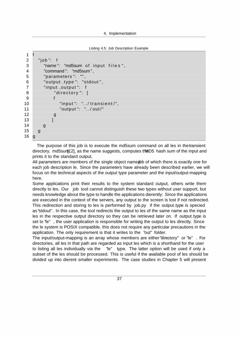
4. Implementation
Listing 4.5: Job Description Example
1 {2 ”job ”: {3 ”name ”: ”md5sum of input f i l e s ” ,4 ”command ”: ”md5sum” ,5 ”parameters ”: ”” ,6 ”output type ”: ”stdout ” ,7 ”input output ”: {8 ”d i r e c t o r y ”: [9 {
10 ”input ”: ”. . / t r a n s i e n t /” ,11 ”output ”: ”. . / out /”12 }13 ]14 }15 }16 }
The purpose of this job is to execute the md5sum command on all files in the transientdirectory. md5sum [12], as the name suggests, computes the MD5 hash sum of the input andprints it to the standard output.All parameters are members of the single object named job of which there is exactly one foreach job description file. Since the parameters have already been described earlier, we willfocus on the technical aspects of the output type parameter and the input/output-mappinghere.Some applications print their results to the system standard output, others write themdirectly to files. Our job tool cannot distinguish these two types without user support, butneeds knowledge about the type to handle the applications differently: Since the applicationsare executed in the context of the servers, any output to the screen is lost if not redirected.This redirection and storing to files is performed by job.py if the output type is specifiedas ”stdout”. In this case, the tool redirects the output to files of the same name as the inputfiles in the respective output directory so they can be retrieved later on. If output type isset to ”file”, the user application is responsible for writing the output to files directly. Sincethe file system is POSIX compatible, this does not require any particular precautions in theapplication. The only requirement is that it writes to the ”out” folder.The input/output-mapping is an array whose members are either ”directory” or ”file”. Fordirectories, all files in that path are regarded as input files which is a shorthand for the userto listing all files individually via the ”file” type. The latter option will be used if only asubset of the files should be processed. This is useful if the available pool of files should bedivided up into different smaller experiments. The case studies in Chapter 5 will present
37

4. Implementation
examples for this kind of job description.
4.3.3. Functions
4.3.3.1. init
As in the case of cluster.py, the init function here also serves to initialize a new object,in this case a job. This operation consists of just two steps:
1. Creating a sub-directory in the invisible .job config with the name of the newly createdjob.
2. Placing a job description template in the .job config directory.
The job template contains no runnable description, but is well structured and containsall parameters to ease adaptation by the user before starting the job.
4.3.3.2. start
The start operation is the most complex one of the job tool involving logic on both theclient and server side which we will explain separately.
Client Side First, start parses the job description file and checks whether its input/output-mapping is valid. While this mapping may by design include both, directories and filessections, the server side – for reasons to be explained in the next paragraph – requires afile-based mapping. This conversion is performed upon job start to incorporate any changesthat the user may have made to the job description. Technically, file entries are simplycopied into an associative array and the directory entries are converted into file entries byscanning the directory’s contents and creating an entry in the array for each file found.job.py then serializes this associative array for later transfer to the cluster.
Second, using the parameters from the job description, the function creates a Python scriptfrom a template that will later serve as the Hadoop Streaming mapper script. See belowfor a discussion of this script.
Lastly, the Ansible job start.yml playbook (Appendix B.4) is launched. The first part of theplaybook synchronizes the project files to the cluster, more specifically just the transientdirectory. The second part launches the Hadoop Streaming job which marks the transitionto the server side.
38

4. Implementation
Server Side We begin our description of the server side job execution with the correspond-ing Hadoop call:
Listing 4.6: Server-side Job Execution
1 / opt /hadoop/ bin /hadoop j a r / opt/hadoop/ share /hadoop/ t o o l s / l i b /hadoop−streaming −*. j a r
2 −D mapreduce . map . cpu . vcore s=23 −input /{{ project name }}/ . j o b c o n f i g /{{ job }}/
i n p u t l i s t . txt4 −output /mr tmp5 −mapper /mnt/ hdfs /{{ project name }}/ . j o b c o n f i g /{{ job
}}/ mr job . py6 −inputformat org . apache . hadoop . mapred . l i b . NLineInputFormat7 && touch /mnt/ hdfs /{{ project name }}/ . j o b c o n f i g / jobdone
Line 1 references the JAR file for Hadoop Streaming. Line 2 assigns each map task twocores. As described in Section 2.4.3, Hadoop expects an input and an output location.In this case (line 4), the output directory is a dummy, because we are not interested inHadoop’s diagnostic output. The input parameter refers to a file created on the client side,which simply lists line by line the files that should be processed and thus equals keys of theserialized associative array discussed above. This array is used in the mapper script specifiedin line 5 (more on that below), but cannot be used as the input parameter because it doesnot comply with any of the supported file types. Of these, we chose the NLineInputFormatinstead of the default TextInputFormat, because it ensures that each map task receives justone input file and each a separate one which is what we need for optimal distribution of theworkload. Finally, upon successful execution of the Hadoop job, the jobdone file is createdas an indicator for job.py that the output can be downloaded. The variables in the call –identifiable by their encapsulation in double curly braces – are replaced by Ansible prior toexecution.
From the start of the Hadoop job on it remains in charge of managing the different mapprocesses, monitoring the overall progress, failure handling et cetera, but the actual execu-tion of the user application is encapsulated in the mapper script which will be discussednow. A version shortened to the key parts is shown in Listing 4.7.
Listing 4.7: Mapper Script
1 . . . module imports . . .2 . . . v a r i a b l e d e c l a r a t i o n s . . .34 i o m a p p i n g f i l e = open( ’ /mnt/ hdfs / $ p r o j e c t / . j o b c o n f i g / $job /
io mapping . p i c k l e ’ , ’ r ’ )
39

4. Implementation
5 io mapping = p i c k l e . load ( i o m a p p i n g f i l e )67 for task in sys . s td in :8 ( key , task ) = task . r s t r i p ( ) . s p l i t ( ’ \ t ’ )9
10 # Bui ld t a s k command11 cmd = command + ’ ’ + parameters + ’ ’ + task12 i f output type == ’ stdout ’ :13 cmd += ’ > ’ + io mapping [ task ]1415 # Execute t a s k16 s t a t u s = os . system (cmd)1718 os . system ( ’ cp /tmp/ l o c a l j o b o u t /* %s ’ % os . path . j o i n ( p r o j e c t d i r ,
’ out ’ ) )
Line 4-5 open the serialized input/output-mapping and deserialize it. Importantly, thefile string in line 4 is modified prior to the execution as $project and $job are variables. Thereplacement of these variables with the true values occurs on the client side prior to the jobexecution. The mapper script receives its input from Hadoop via the STDIN channel. TheStreaming call above implies that each mapper process normally receives just one inputfile. However, for fail safety the script iterates over its input (line 7) to be able to dealwith multiple input files loop-wise. Due to the choice of NLineInputFormat as the inputformat, the mapper receives not just the file name from the input list, but a key/value pairseparated by a tabular character with the key corresponding to the character position of theinput list (line 8). The remainder of the for loop prepares the call to the user applicationand executes it. Line 13 marks the different treatment depending on the output type of theapplication: If the user application prints to STDOUT, the command line call arranges forthe output redirection into the file name specified by the user in the input/output-mapping(line 13). Finally, after the user application has exited (line 16), the script copies the locallycached output files to the HDFS so that all node’s output files are available at a commonlocation.
4.3.3.3. download
The download function allows the user to retrieve the output files generated by her job run.The download needs to be implemented as a pull operation (i.e., the user initiates the datatransfer) separate from the job execution, because the job may finish at a time when theuser’s machine is not running and the data could not be transferred if that is the case.The download operation uses an Ansible play shown in Appendix B.4.
40

4. Implementation
Listing 4.8: Ansible File for Result Download
1 −−−2 # job −−download play34 − hos t s : namenode5 remote user : root6 sudo : yes7 sudo user : hadoop8 ta sk s :9 − s t a t : path=/mnt/ hdfs /{{ project name }}/ . j o b c o n f i g / jobdone
10 r e g i s t e r : jobdone11 − f a i l : msg=”Job has not f i n i s h e d yet ”12 when : not jobdone . s t a t . e x i s t s13 − synchron ize : mode=p u l l s r c=/mnt/ hdfs /{{ project name }}/ out
dest={{ pro j e c t pa th }}14 when : jobdone . s t a t . e x i s t s
Prior to the tasks, the Ansible file specifies that it should work with the namenode machineand be executed as the user hadoop, which is the user that also runs the Hadoop services.The actual tasks section employs three different Ansible modules. First, stat checks whetherthere exists a file called jobdone in the project directory and registers the result of the checkin a variable of the same name. The jobdone file is created after the job run has finishedand thus tells job.py if the download may be started. If the result of the check is negative,Ansible aborts with a message that the job has not finished yet. Otherwise, synchronizeperforms a pull operation, syncing the project’s out folder on the server side to the client’smachine.
4.3.3.4. delete
The delete operation solely removes local traces of a configured job, i.e. its directory andjob description file in .job config.
41

5. Case Studies
In this chapter we will examine the practicability of our approach with the help of twoapplications written by researchers of the group of Software Engineering for Dis-tributed Systems. We chose these two applications because they represent real-worlduse cases for our approach and therefore they can provide realistic results for the judgementof the feasibility of our work. We will begin with the description of our test environmentin Section 5.1. Following, in Section 5.2 we will discuss the metrics with which we evaluatethe performance of our approach. The remainder of the chapter will then cover the two casestudies and their results (Sections 5.3 and 5.4).
5.1. Environment
5.1.1. Cluster Specifications
For mainly two reasons, we chose the Compute Cloud service of the GWDG as the Cloudservice for our evaluation. The first reason is that the GWDG is the main provider of ITservices for the University of Gottingen. Therefore, should the approach turn out to beuseful and also generalizable enough, it may be interesting for other local researchers forwhom the Compute Cloud is possibly the most cost-effective choice. The second reason isthat research grants of e.g. Amazon are no longer as easily available as in the past andthere were no resources available for purchasing commercial Cloud resources for this thesis.The GWDG provided an account with an initial quota of 10 virtual machines of a customflavour which was later on extended to 15 for testing the deployment of a second clusternext to an existing one.In expectation of possibly large data sets, the storage-rich private flavour hadoop was createdfor us with the specifications listed in Table 5.1.
Virtual CPUs 2 CoresMemory 4GB RAMStorage 275GB HDDArchitecture 64 bit
Table 5.1.: Hadoop Flavour
42

5. Case Studies
Our evaluations were performed on a cluster consisting of 10 machines of this flavour.Naturally, using a different flavour with other characteristics would yield different results,which may be better or worse depending on the respective user application. However,the rationale of our evaluation was not to find the best suited infrastructure for our casestudies, but to execute them in an average setup to explore the performance in non-optimizedconfigurations.
5.1.2. Software Versions
We here list the versions of all software that we used and deem directly relevant. Noteworthy,while our approach may be more sensible to changes in some software than in other, it shouldnot be affected by minor or even major version changes due to the backward compatibilityin the underlying foundations. Table 5.2 lists the software.
Software Versions
Hadoop 2.5.2Ansible 1.9Vagrant 1.6.5Java OpenJDK 1.7.0Python 2.7.6Linux Ubuntu Server 14.04
Table 5.2.: Environment Software Versions
5.2. Metrics
The most widely used metric to express the relative performance gain from parallelizationof a task is the speedup which is defined as[58]:
Speedup = Execution timeoldExecution timenew
where the old execution time is the wall-clock time for executing the entire task without par-allelization and the new execution time the duration with parallelization. Ideally – ignoringcases of super-linear speedup irrelevant for our case – the speedup for p processors/nodes isitself p, meaning that for p nodes the execution time reduces to 1/p.We will employ the speedup as our main and only metric for the following reasons:
� Most importantly, the speedup is the metric motivating this thesis, i.e. we want toevaluate how much speedup can be gained with no effort on the user side. Again, weare interested in the wall-clock time, because it is the metric of interest for the user.
43
5. Case Studies
� Other metrics such as the average utilization of the infrastructure depend too much onthe particular use case. As an example, given a fixed cluster size of n it is obvious thata job with m input files where m < n, the cluster cannot possibly be fully utilized,without this being a drawback of our approach. Even with m > n, the utilizationdepends primarily on the degree of input heterogeneity, as will become clear from thediscussion of our case studies.
� Yet other low-level metrics such as the communication overhead which is of intereste.g. in message-passing parallelization are neither measurable nor of interest herebecause – being determined by Hadoop – they are out of scope of our implementation,thus not improvable and implicitly a determinant of the overall speedup.
Our evaluation of the speedup, here being the quotient of the execution time on just onenode (i.e. the time of non-parallelized execution) and the time of a parallelized job in thecluster, will investigate if it is beneficial to use our approach in terms of reduced executiontimes and quantify this for different scenarios.
5.3. CrossPare
5.3.1. Application Description
CrossPare is an application developed by one supervisor of this thesis, Steffen Herbold,that employs machine learning algorithms on software project data to identify potentiallyerroneous application components. More specifically, it takes as input data from the Tera-Promise repository [42] that collects metrics from the different components of a poolof open-source projects on the source code level as well as the information whether eachcomponent contains bugs or not. Examples for such metrics are the lines of code (LOC) orthe number of methods in a class. By feeding this data into a set of configurable machinelearning algorithms, CrossPare attempts to identify the most predictive metrics. Dependingon the type and number of selected algorithms – which are defined in so-called experiments –the run time can vary substantially. We will describe this in more detail in the next section.The application directory structure had to be slightly adjusted to fit our requirementsdetailed in Section 3.3.1. However, since the application has no hard-coded input/output-mapping defined in its code, but rather reads it from its input files, the restructuring merelyinvolved some file moves and slight modifications to the experiments, but no changes on thesource code level.
Figure 5.1 depicts the directory organization after the restructuring. crosspare.jar as theapplication’s JAR file resides in fixed along with a directory containing libraries it dependson (lib) and the data directory that contains the input data. The experiments are stored ina sub-directory of transient because there may be changes to the pool of experiments. Forexample, an algorithm may be regarded as unnecessary after the first run or new experiments
44

5. Case Studies
Figure 5.1.: CrossPare Directory Structure
may be added, while the application itself remains unchanged.Finally, it is important to note that CrossPare uses thread-level parallelization, i.e. eachprocess launches as many threads as there are CPU cores if the number of input files tothat process is large enough. Thus, for a dual core machine with two or more input files,two threads will be started. This fact will be important in our evaluation.
5.3.2. Evaluation Setup
As mentioned above, experiments are defined in XML files. Listing 5.1 shows exemplarilyone of the experiment configurations we examined. Important for our discussion are the lines3 and 13 as well as 9-12. The prior define the input and output data locations and markthose parameters that needed to be adapted to match our directory structure. The latterlines define the trainers, i.e. the machine learning classification algorithms, that should beapplied to the input data.
Listing 5.1: Experiment Configuration (SMALL1)
1 <?xml version=”1 .0 ” encoding=”UTF−8”?>2 <c o n f i g xmlns=”exper imentcon f ig ” xmlns :x s i=”h t tp : //www. w3 . org
/2001/XMLSchema−i n s t anc e ” xs i : s chemaLocat ion=”exper imentcon f igexper imentcon f i g . xsd ”>
3 <l o ade r name=”CSVFolderLoader ” d a t a l o c a t i o n=” . . / f i x e d / data ”r e l a t i v e=” f a l s e ”/>
4 <v e r s i o n f i l t e r name=”MinClassNumberFilter ” param=”5 ” />5 <s e t w i s e p r e p r o c e s s o r name=”Normal izat ion ” param=””/>6 <s e t w i s e p r e p r o c e s s o r name=”AverageStandardizat ion ” param=”” />7 <s e t w i s e p o s t p r o c e s s o r name=”Undersampling ” param=”” />8 <p o s tp r o c e s s o r name=”Undersampling ” param=”” />9 <t r a i n e r name=”WekaTraining ” param=”RandomForest weka . c l a s s i f i e r s .
t r e e s . RandomForest −CVPARAM I 5 25 5 ” />
45

5. Case Studies
10 <t r a i n e r name=”WekaTraining ” param=”C4.5−DTree weka . c l a s s i f i e r s .t r e e s . J48 −CVPARAM C 0.1 0 .3 5 ” />
11 <t r a i n e r name=”WekaTraining ” param=” L o g i s t i c weka . c l a s s i f i e r s .f u n c t i o n s . L o g i s t i c ” />
12 <t r a i n e r name=”WekaTraining ” param=”NeuralNetwork weka . c l a s s i f i e r s. f u n c t i o n s . Mul t i l ayerPerceptron −CVPARAM M 1.5 2 .5 3 .0 L 0 .20 .4 3 .0 ” />
13 <r e s u l t s p a t h path=” . . / out/ r e s u l t s ”/>14 <eva l name=”NormalWekaEvaluation ” param=”” />15 </ c o n f i g>
The computational complexity of these trainers is extremely heterogeneous, ranging fromless than a minute to hours. For example, the logistic regression algorithm finishes a lotfaster than the neural network given the parameters from the experiment. For the purposeof our evaluation, we define three experiments: SMALL, MEDIUM and LARGE. The first,as already shown in 5.1 consists of four trainers with varying run times. MEDIUM doublesthe trainers, LARGE quadruples them.For the sake of comparing performance in different scenarios, we define the following cases:
1. 2x SMALL
2. 4x SMALL
3. 8x SMALL
The rationale for the first case is to measure the overhead induced by our approach. Ifthe overhead was zero, the execution time on one machine with two times the SMALLexperiment as input should be as fast as the parallelization to two nodes. This may becounterintuitive at first, because the execution on two nodes should ideally be twice as fast.However, as each map task receives just one input file, it cannot make use of the thread-level parallelism in CrossPare and thus each node takes approximately the same time for theprocessing of two input files as for one. We will discuss this shortcoming in the conclusion.
The rationale for the second and third case are to measure the speedup for parallelizingto four or eight nodes. Ideally, the execution time should have between 2x SMALL and4x SMALL and again between 4x and 8x. The other two experiment files, MEDIUM andLARGE are not part of our evaluation in this section. Instead, they will play a role in thecomparison with a native MapReduce implementation in Chapter 6.
5.3.3. Results
We execute each case parallelized via our approach and non-parallelized on just one machine.For consistent results, we chose one virtual machine of the cluster as the reference setup
46
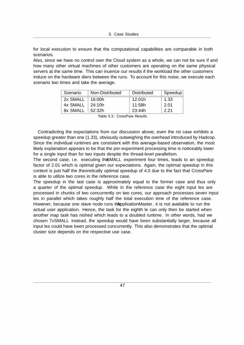
5. Case Studies
for local execution to ensure that the computational capabilities are comparable in bothscenarios.Also, since we have no control over the Cloud system as a whole, we can not be sure if andhow many other virtual machines of other customers are operating on the same physicalservers at the same time. This can influence our results if the workload the other customersinduce on the hardware differs between the runs. To account for this noise, we execute eachscenario two times and take the average.
Scenario Non-Distributed Ø Distributed Ø Speedup
2x SMALL 16:00h 12:01h 1.334x SMALL 24:10h 11:58h 2.018x SMALL 52:32h 23:44h 2.21
Table 5.3.: CrossPare Results
Contradicting the expectations from our discussion above, even the first case exhibits aspeedup greater than one (1.33), obviously outweighing the overhead introduced by Hadoop.Since the individual runtimes are consistent with this average-based observation, the mostlikely explanation appears to be that the per-experiment processing time is noticeably lowerfor a single input than for two inputs despite the thread-level parallelism.The second case, i.e. executing the SMALL experiment four times, leads to an speedupfactor of 2.01 which is optimal given our expectations. Again, the optimal speedup in thiscontext is just half the theoretically optimal speedup of 4.0 due to the fact that CrossPareis able to utilize two cores in the reference case.The speedup in the last case is approximately equal to the former case and thus onlya quarter of the optimal speedup. While in the reference case the eight input files areprocessed in chunks of two concurrently on two cores, our approach processes seven inputfiles in parallel which takes roughly half the total execution time of the reference case.However, because one slave node runs the ApplicationMaster, it is not available to run theactual user application. Hence, the task for the eighth file can only then be started whenanother map task has finished which leads to a doubled runtime. In other words, had wechosen 7x SMALL instead, the speedup would have been substantially larger, because allinput files could have been processed concurrently. This also demonstrates that the optimalcluster size depends on the respective use case.
47

5. Case Studies
5.4. TaskTreeCrossvalidation
5.4.1. Application Description
Our second case study, for the lack of an official name here referred to asTaskTreeCrossvalidation, is an application written by a researcher of the SoftwareEngineering for Distributed Systems group in the context of his PhD thesis, PatrickHarms. Again, we will briefly introduce the background of the application before discussingthe adaptations needed to be compatible with our approach.Harms research is partially concerned with the usability analysis of websites. Part of this isthe use of so-called task trees to formally describe user interactions in a tree structure whereparent nodes define the order of actions and leaf nodes the actual actions performed by theuser, called tasks (e.g. clicks, text input etc.). The rationale for the trees is to analyse themlater on to detect potential usability issues [57] [56]. The recording of the user actions isperformed using the AutoQUEST tool suite [6].The application for our case study is an intermediate tool that verifies whether the trees theapproach generates are similar trees for different recordings of the same website, becauseotherwise they would not be considered suitable for the usage analysis.The changes needed to the application for the use with our approach were small, especiallyin terms of the application structure. Basically, there is only one folder structured as follows:
� autoquest-distribution: Contains the AutoQUEST tool suite with the verification code.
� run.sh: A wrapper script for executing AutoQUEST.
� crossvalidation.data: The recording of the user interactions.
� Script files: Configuration files that instruct run.sh. Equivalent to the experimentconfiguration files of CrossPare.
The structure could remain the same for execution with our framework, though moving theexperiment configurations to the transient directory is recommended for reasons explainedearlier. However, because no changes to the files were planned for the course of the casestudy and to demonstrate that our approach can be used with minimal overhead, we leftthe structure as is.Before planning of the case study, run.sh relied heavily on command line switches for therun configurations. Since our approach assumes the same parameters for all runs, this posesa problem because all run-specific informations need to be passed via the input file. Toaccount for this, TaskTreeCrossvalidation has been modified as to receive its configurationvia one single file, the script file.
48

5. Case Studies
5.4.2. Evaluation Setup
The runtime of the application is determined by the complexity of the experiment defined inthe input file. More specifically, depending on the experiment configuration, the applicationneeds to perform more or less task tree comparisons on the data set. The size of theexperiment is expressed as the percentage of the data set which is used to generate the tasktrees for comparison, e.g. crossvalidation 10 1 script (Listing 5.2) defines an experimentwhere task trees are generated and compared for 10% subsets of the data.
Listing 5.2: TaskTreeCrossvalidation Configuration Example
1 load . . / c r o s s v a l i d a t i o n . data2 generateTaskTree s equence s subse t 10 1 t a s k t r e e s u b s e t 1 0 13 generateTaskTree s equence s subse t 10 2 t a s k t r e e s u b s e t 1 0 24 getTaskMode lS imi lar i ty t a s k t r e e s u b s e t 1 0 1 t a s k t r e e s u b s e t 1 0 25 save . . / . . / out/ c r o s s v a l i d a t i o n 1 0 1−r e s u l t s . data6 e x i t
The larger the subsets, the more comparisons are needed and the longer the executiontime. Subset sizes in the distribution provided to us range from 1% to 20%. Further-more, in addition to the crossvalidation * experiment configurations, there are crossvali-dation fullrecall * files that compares the subsets with the full dataset, leading to a sub-stantially longer runtime. For our case study, we define two scenarios for evaluating ourapproach’s performance:
1. The heterogeneous case: Consists of each two times 1%, 2.5%, 5% and 10% sizeexperiment configurations, i.e. 8 input files in total.
2. The homogeneous case: Consists of 6 input files in total, but this time only 10%experiment configurations.
The rationale for the two cases is to evaluate whether there is a difference in the speedupfor heterogeneous and homogeneous experiments. This contrasts our first case study whereinstead of evaluating differently structured inputs, we examined the use of a varying numberof input files, i.e. a different number of parallel processes.
5.4.3. Results
We perform the evaluation in the same fashion as in our first case study. To measure thereference (i.e. non-parallelized) performance, we execute the application on one machine ofour cluster and repeat both the reference and parallel case to mitigate the effects of volatileCloud performance. Table 5.4 summarizes the results.
49

5. Case Studies
Scenario Non-Distributed Ø Distributed Ø Speedup
Heterogeneous Input 4:24h 2:02h 2.16Homogeneous Input 9:57h 2:10h 4.57
Table 5.4.: TaskTreeCrossvalidation Results
As can be seen from the table, our approach processes both scenarios faster than thenon-distributed execution. However, the speedup is twice as large for the homogeneouscase compared to the heterogeneous case. The explanation for this circumstance is simple:In both cases, six worker nodes are each assigned one of the input files. While in theheterogeneous case the smaller experiments finish after just some minutes and the respectivenodes are then in an idle state, in the homogeneous case the nodes are all utilized forapproximately the same time, leading to a higher average utilization and thus to a higherspeedup.The situation for the heterogeneous case would improve with an increased problem size.Assuming that each input file exists e.g. ten times, the average utilization of each workernode would also increase, because once the smaller input configurations have been processed,there were still larger ones in the queue.
50

6. Comparison with MapReduce
In the approach we presented in the previous chapters, we have utilized Hadoop Streamingas a wrapper to MapReduce for executing arbitrary applications. The results of our casestudies were promising with regard to the possible runtime reductions involved in usingour approach. In this chapter, we are going to compare these results with that of a nativeMapReduce application.Section 6.1 will present general considerations needed for transforming an application intoa MapReduce application. It is important to note that while we try to keep them as generaland high-level as possible, they will not apply to any potential application. Section 6.2,following this guideline, shows the steps involved in porting the CrossPare application.Finally, in Section 6.3, we compare its performance with both the non-distributed executionand with the execution via our Streaming-based approach.
6.1. General Considerations
In this section we attempt to generalize the procedure of parallelizing an existing applicationusing MapReduce in the form of a few general steps that should be executed in the respectiveorder. Naturally, applications vary a lot in terms of many dimensions such as their intendedpurpose, program structure, employed libraries et cetera and not all applications will becompatible with the schema presented. To start with the most basic level, the software willneed to be implemented in Java to use Hadoop’s API.Following, we will describe the 6 steps we identified on a high-level basis prior to showingtheir implementation in CrossPare, one of our case study applications.
1. Identify Parallelizable Tasks The perhaps most critical step is the identification of par-allelizable tasks in the software. This is not only of concern for our context, but for appli-cation parallelization in general. Naturally, strictly sequential (atomic) operations cannotbe distributed across different nodes because each of them depends on the result of the op-erations preceding it. Therefore, the developer needs to identify self-contained tasks whoseexecution process is independent of others.Also, as a second criterion, the identified tasks should be complex enough to qualify forparallelization. Complex enough here means (1) that the runtime of the tasks accountsfor a non-negligible share of the overall runtime of the application and (2) that each task’s
51

6. Comparison with MapReduce
runtime justifies the overhead involved in distributing them. The rationale for the firstrequirement is that it only when it is fulfilled, there is a possibility to substantially reducethe application’s runtime. The second requirement arises from the fact that parallelizationitself comes with an overhead (most importantly communication), that, if it is too largecompared to the gains of distributed processing, leads to an increased overall runtime in-stead of a reduction. The Hadoop documentation recommends a minimum map task timeof one minute [26].
2. Identify Needed Objects Technically, MapReduce tasks run in their own JVM andhave no access to the object space of the user application. This has severe implications for theparallelization of tasks because the developer needs to think of the map tasks as independentprograms that need to receive input from the calling application in a substantially differentway than e.g. simply calling a Java method.We call this this input ”objects”, because the Java objects the mapper class needs are thefundamental entity: While static input data to the application such as experiment data canbe read by the mapper class directly from the shared file system (HDFS) and parametersof certain types (e.g. Strings) can be passed via the Hadoop API, objects of other types ofthe user application that are needed for performing the tasks to be parallelized cannot beaccessed directly, thus establishing the need to identify and transfer these explicitly.Which parts of the program these are exactly can hardly be generalized in a satisfactoryway. Our example in the next section will shed more light on this step.
3. Serialize Objects We noted in the previous step that the map tasks share access toHadoop’s filesystem. Consequently, it is also predestined to provide the storage for thepreviously identified objects to the corresponding map tasks. The de-facto standard toshare objects between processes is to serialize them, i.e. converting their state to a bytestream adhering to a certain specification which can be transformed back into the sameobject [29]. By serializing the identified objects and storing them in files in the HDFS, themap tasks gain access to their required input.
4. Implement Mapper Class As explained in the overview on the MapReduce paradigmin Section 2.4.1, at the very least a map function is required for each MapReduce application.In Hadoop’s API, this function is embedded in classes that implement the Mapper interface.In this context, the mapper class is responsible for the processing of the parallelized taskand thus contains all code related to its execution.Its schema can be described as (1) Deserialize (2) Process (3) Serialize: In step (1), the mapfunction deserializes the previously serialized objects to use them in (2) for processing thetask and (3) serializing the result for later use in the user application.
52
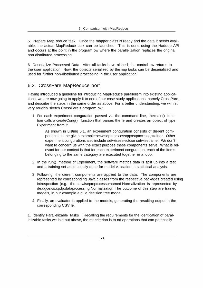
6. Comparison with MapReduce
5. Prepare MapReduce task Once the mapper class is ready and the data it needs avail-able, the actual MapReduce task can be launched. This is done using the Hadoop APIand occurs at the point in the program flow where the parallelization replaces the originalnon-distributed processing.
6. Deserialize Processed Data After all tasks have finished, the control flow returns tothe user application. Now, the objects serialized by the map tasks can be deserialized andused for further non-distributed processing in the user application.
6.2. CrossPare MapReduce port
Having introduced a guideline for introducing MapReduce parallelism into existing applica-tions, we are now going to apply it to one of our case study applications, namely CrossPare,and describe the steps in the same order as above. For a better understanding, we will firstvery roughly sketch CrossPare’s program flow:
1. For each experiment configuration passed via the command line, the main() func-tion calls a createConfig() function that parses the file and creates an object of typeExperiment from it.
� As shown in Listing 5.1, an experiment configuration consists of different com-ponents, in the given example: setwisepreprocessor, postprocessor, trainer. Otherexperiment configurations also include setwiseselector or setwisetrainer. We don’twant to concern us with the exact purpose these components serve. What is rel-evant for our context is that for each experiment configuration, each of the itemsbelonging to the same category are executed together in a loop.
2. In the run() method of Experiment, the software metrics data is split up into a testand a training set as is usually done for model validation in statistical analysis.
3. Following, the different components are applied to the data. The components arerepresented by corresponding Java classes from the respective packages created usingintrospection (e.g. the setwisepreprocessor named Normalization is represented byde.ugoe.cs.cpdp.dataprocessing.Normalization). The outcome of this step are trainedmodels, in our example e.g. a decision tree model.
4. Finally, an evaluator is applied to the models, generating the resulting output in thecorresponding CSV file.
1. Identify Parallelizable Tasks Recalling the requirements for the identification of paral-lelizable tasks we laid out above, the first criterion is to find operations that can potentially
53
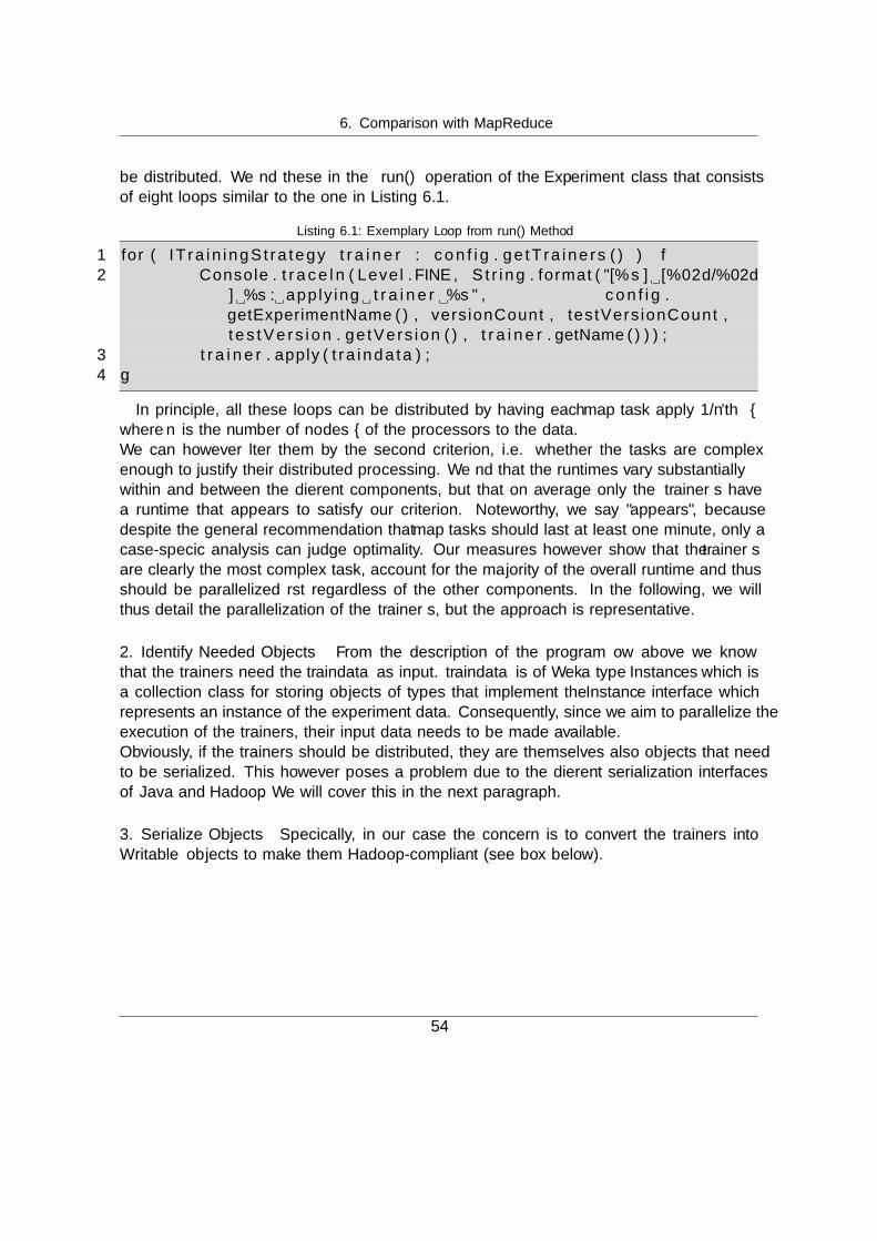
6. Comparison with MapReduce
be distributed. We find these in the run() operation of the Experiment class that consistsof eight loops similar to the one in Listing 6.1.
Listing 6.1: Exemplary Loop from run() Method
1 for ( ITra in ingSt ra tegy t r a i n e r : c o n f i g . g e tTra ine r s ( ) ) {2 Console . t r a c e l n ( Leve l . FINE , St r ing . format ( ”[%s ] [%02d/%02d
] %s : apply ing t r a i n e r %s ” , c o n f i g .getExperimentName ( ) , versionCount , testVers ionCount ,t e s t V e r s i o n . getVers ion ( ) , t r a i n e r . getName ( ) ) ) ;
3 t r a i n e r . apply ( t ra inda ta ) ;4 }
In principle, all these loops can be distributed by having each map task apply 1/n’th –where n is the number of nodes – of the processors to the data.We can however filter them by the second criterion, i.e. whether the tasks are complexenough to justify their distributed processing. We find that the runtimes vary substantiallywithin and between the different components, but that on average only the trainers havea runtime that appears to satisfy our criterion. Noteworthy, we say ”appears”, becausedespite the general recommendation that map tasks should last at least one minute, only acase-specific analysis can judge optimality. Our measures however show that the trainersare clearly the most complex task, account for the majority of the overall runtime and thusshould be parallelized first regardless of the other components. In the following, we willthus detail the parallelization of the trainers, but the approach is representative.
2. Identify Needed Objects From the description of the program flow above we knowthat the trainers need the traindata as input. traindata is of Weka type Instances which isa collection class for storing objects of types that implement the Instance interface whichrepresents an instance of the experiment data. Consequently, since we aim to parallelize theexecution of the trainers, their input data needs to be made available.Obviously, if the trainers should be distributed, they are themselves also objects that needto be serialized. This however poses a problem due to the different serialization interfacesof Java and Hadoop. We will cover this in the next paragraph.
3. Serialize Objects Specifically, in our case the concern is to convert the trainers intoWritable objects to make them Hadoop-compliant (see box below).
54

6. Comparison with MapReduce
Java vs. Hadoop Serialization
Java and Hadoop employ different serialization implementations which differ both intheir underlying storage and in their user-visible interface. CrossPare contains mul-tiple trainer classes for different purposes which all implement the ITrainingStrategyinterface and extend the WekaBaseTraining class, but which are also differ in theirsuitability for being serialized as Writables.In Java, classes need to implement the java.io.Serializable [30] interface. Giventhis and that all of its members themselves are serializable or marked as be-ing transient, this suffices to serialize objects of the class using an ObjectOutput-Stream. In the case of Hadoop, classes that should be serializable implement theorg.apache.hadoop.io.Writable [21] interface. Noteworthy, all objects that appear asinput or output in map or reduce operations need to be serializable. While in Java se-rialization no further methods need to be implemented, the Hadoop interface expectsthe developer to add the void write(DataOutput out) and void readFields(DataInputin) to the class. The latter’s purpose is to serialize the fields of the object to thegiven DataOutput stream, while the first is the reverse operation, i.e. it deserializesthe fields of the object. A crucial limitation of DataOutput is that its write operationsare limited to Java’s primitive types. This implies that user-defined classes cannotusually be serialized without effort. The two operations are typically complementedby a third static method read(DataInput in) that instantiates an object of the classand calls readFields() on it to populate the object.This relates to the internal differences in both approaches. Java does not assume thatthe class of the stored objects is known, Hadoop on the other hand does assume thisbecause the application creates the instance of the class before calling readFields().Therefore, because the type of the object does not have to be stored in the bytestream, Hadoop serialization is less input/output-intensive. Since MapReduce is veryinput/output-intensive due to the fact that objects regularly need to be transferredacross the network, reducing the required communication is paramount. [19]The differences outlined here have the important implication that both serializationapproaches are not interchangeable, therefore not allowing plain Serializable classesto be used in the context of Hadoop operations.
This is due to the way they are implemented: Some of the classes contain inner classes andmultiple class members, making it hard to serialize them in this scheme. More concretely,part of the problem is that because Hadoop’s DataOutput supports only primitive types,complex types need to be converted into one of these types first, e.g. a byte array. This,however, requires a prior serialization of the object using Java’s serialization which again isonly practicable for classes supporting it, which does not apply to all of those used in the
55

6. Comparison with MapReduce
trainer classes.Hence, to avoid making substantial changes to CrossPare, we have to limit ourselves tothe WekaTraining class that does not add any additional members to its base class (Wek-aBaseTraining) and thus only contains the members as depicted in Figure 6.1. Though thistrainer does not cover all experiments in use with CrossPare, it covers a great part of themand thus a speedup-involving distribution of them would contribute to an overall runtimeimprovement.
Figure 6.1.: WekaBaseTraining Class Diagram
We split up our discussion of the serialization into two parts, the training data and theactual trainers. Finally, we will show how to make the serialized data available to theMapReduce portion of the program.
Training dataWe recall that traindata is of type weka.core.Instances which is a Java Serializable becauseWeka has been designed to support serialization in its core types. Since the training data isrelevant to all of our map tasks instead of just a specific one as in the case of the trainers, weaim to make it available globally. Hadoop supports this via its concept of the Configurationobject used for setting up a job. This object can be assigned values via its set(String name,String value) operation. In our case, we can utilize this concept in the following way:
1. Convert the instances to a ByteArrayOutputStream via an ObjectOutputStream.
2. Convert this byte array to a Base64 String using the Apache Commons library [4].
56

6. Comparison with MapReduce
3. Set this string as the value for the configuration option ”traindata”.
Now, this serialized version of the training data is available to all map tasks. We will seehow the mapper class accesses it in the next paragraph.
TrainersThe second class of objects to serialize are the trainers. Listing 6.2 shows the correspondingcode.
Listing 6.2: Serialization of Trainers
1 ArrayList<Str ing> i n p u t F i l e s = new ArrayList<Str ing >() ;2 for ( ITra in ingSt ra tegy i : c o n f i g . g e tTra ine r s ( ) ) {3 WekaTraining t r a i n e r = ( WekaTraining ) i ;4 try {5 St r ing f i l ename = Long . t oS t r i ng ( System . nanoTime ( ) )
+ ” . s e r ” ;6 Path s e r i a l i z a t i o n F i l e = new Path (
s e r i a l i z a t i o n T r a i n e r I n p u t D i r , f i l ename ) ;7 OutputStream os = f s . c r e a t e ( s e r i a l i z a t i o n F i l e ) ;8 os . wr i t e ( S e r i a l i z a t i o n H e l p e r . s e r i a l i z e ( t r a i n e r ) ) ;9 os . c l o s e ( ) ;
10 i n p u t F i l e s . add ( s e r i a l i z a t i o n F i l e . t oS t r i ng ( ) ) ;11 } catch ( Exception e ) {12 System . out . p r i n t l n ( ”Exception s e r i a l i z i n g
to d i sk : ” + e ) ;13 }14 }
We iterate over the trainers and cast them to WekaTraining by our assumption that we onlyuse trainers of that type in this context. Our aim is to serialize the trainers to HDFS-backedfiles that can be read by the map tasks. The order is arbitrary, so a random filename (line 5)suffices, for which the corresponding HDFS path is setup (line 6) and OutputStream opened(line 7). The trainer then gets serialized and the resulting binary stream is written to thefile (line 8). Finally, the file is added to the list of filenames that should be processed. TheSerializationHelper class called in line 8 is simply a helper class for wrapping the serializa-tion to and deserialization from Writables (see Appendix B.5). For brevity, we don’t showthe corresponding write() and readFields() of the WekaTraining class here (see AppendixB.6 for the complete code).
At this point, all needed objects are serialized, notably in different fashion: While thetraining data is available to the Hadoop tasks via its Configuration object, the trainers have
57

6. Comparison with MapReduce
been serialized to disk. Conceptually, we could have serialized the former to disk, too, butnot the other way around. However, since there is an overhead involved in serializing todisk, our approach is preferable and more straightforward to implement.
4. Implement Mapper Class In our context, the task of the mapper class (see AppendixB.7 for the complete class code) is to apply a trainer to the training data and transferback the result of this operation to the program. Like in all Hadoop applications, our classimplements the map() method that is called by the framework. Additionally, we implementthe setup() method which is called once prior to the execution to the actual map operations.
Listing 6.3: setup() Method of TrainerMapper
1 protected void setup ( Context context ) {2 conf = context . g e tCon f i gura t i on ( ) ;3 s e r i a l i z a t i o n T r a i n e r O u t p u t D i r = new Path ( conf . get ( ”
outputpath ”) ) ;4 S t r ing s e r i a l i z e d T r a i n d a t a = conf . get ( ”t ra inda ta ”) ;5 try {6 byte b [ ] = Base64 . decodeBase64 ( s e r i a l i z e d T r a i n d a t a ) ;7 ByteArrayInputStream bi = new ByteArrayInputStream (b) ;8 ObjectInputStream s i = new ObjectInputStream ( bi ) ;9 t ra inda ta = ( In s tance s ) s i . readObject ( ) ;
10 } catch ( Exception e ) {11 System . out . p r i n t l n ( e ) ;12 }13 }
In setup() (Listing 6.3), we retrieve two parameters from the Configuration object of thejob. The first is the path where the processed trainers should be stored. We will discussthis point in the next paragraph. The other parameter is the serialized training data. Line4 reads this data as a Base64-formatted String and deserializes it back with the help ofApache Commons (lines 5-8). The resulting Instances object is assigned to a static variableof the class, thereby making it available to all map tasks.
Listing 6.4: map() Method of TrainerMapper
1 public void map( LongWritable key , Text value , Context context )2 throws IOException , Inter ruptedExcept ion {3 // Read s e r i a l i z e d t r a i n e r from HDFS4 Path i n p u t F i l e = new Path ( value . t o S t r i ng ( ) ) ;5 Fi leSystem f s = FileSystem . get ( conf ) ;6 FSDataInputStream in = f s . open ( i n p u t F i l e ) ;
58

6. Comparison with MapReduce
7 f ina l int a v a i l a b l e = in . a v a i l a b l e ( ) ;8 byte s e r i a l i z e d T r a i n e r [ ] = new byte [ a v a i l a b l e ] ;9 in . readFul ly (0 , s e r i a l i z e d T r a i n e r ) ;
1011 // D e s e r i a l i z e and app ly t r a i n e r12 WekaTraining t r a i n e r = S e r i a l i z a t i o n H e l p e r . asWritable (
s e r i a l i z e d T r a i n e r , WekaTraining . class ) ;13 t r a i n e r . apply ( t ra inda ta ) ;1415 // S e r i a l i z e t r a i n e r and w r i t e to HDFS16 St r ing f i l ename = Long . t oS t r i ng ( System . nanoTime ( ) ) + ” . s e r ” ;17 Path s e r i a l i z a t i o n F i l e = new Path (
s e r i a l i z a t i onTra ine rOutputD i r , f i l ename ) ;18 OutputStream os = f s . c r e a t e ( s e r i a l i z a t i o n F i l e ) ;19 os . wr i t e ( S e r i a l i z a t i o n H e l p e r . s e r i a l i z e ( t r a i n e r ) ) ;20 os . c l o s e ( ) ;21 }
The concept of the map() method is to read a previously serialized trainer from theHDFS, deserialize it, execute it using its apply() method and serialize it back. Notably, theapply() method is the time-intensive task that trains the model. Which trainer the partic-ular map task reads depends on the contents of the value parameter, which is fed in by theHadoop framework. The SerializationHelper again assists in the serialization/deserializationprocess. Processed trainers are saved in the directory specified by the static serialization-TrainerOutputDir with a random file name. By this procedure, the non-distributed partof the application can simply collect the results of the distributed processing as we will seebelow.
5. Prepare MapReduce Job Having the serialized data and the mapper class allows thesetup of a MapReduce job. This setup is performed in the class in which we also serial-ized the needed objects and which usually executes the trainers non-distributedly, namelyExperiment. Listing 6.5 shows our code for the job setup.
Listing 6.5: MapReduce Job Setup
1 Conf igurat ion conf = new Conf igurat ion ( ) ;2 ( . . . t r a i n e r s e r i a l i z a t i o n . . . )34 // Create input index f i l e ( us ing NLineInputFormat )5 Path indexFi lePath = new Path ( s e r i a l i z a t i o n S e q u e n c e I n p u t D i r , ”
input . idx ”) ;
59

6. Comparison with MapReduce
6 OutputStream os = f s . c r e a t e ( indexFi lePath ) ;7 for ( S t r ing f i l ename : i n p u t F i l e s ) {8 f i l ename += ”\n” ;9 os . wr i t e ( f i l ename . getBytes ( ) ) ;
10 }11 os . c l o s e ( ) ;1213 // Job e x e c u t i o n14 conf . s e t ( ”outputpath ” , s e r i a l i z a t i o n T r a i n e r O u t p u t D i r . t o S t r i ng ( ) ) ;15 Job job = Job . g e t In s tance ( conf , ”Weka Tra iner s ”) ;16 job . setJarByClass ( TrainerMapper . class ) ;17 job . setMapperClass ( TrainerMapper . class ) ;18 job . setInputFormatClass ( NLineInputFormat . class ) ;19 NLineInputFormat . addInputPath ( job , s e r i a l i z a t i o n S e q u e n c e I n p u t D i r ) ;20 NLineInputFormat . setNumLinesPerSpl it ( job , 1) ;21 FileOutputFormat . setOutputPath ( job , s e r i a l i z a t i o n O u t p u t D i r ) ;22 job . waitForCompletion ( true ) ;
Line 1 creates the aforementioned instance of the Configuration class. Following, in lines4-10 the input file for the Hadoop job is created by writing the filenames of the serializedtrainers to it separated by newlines. We will not elaborate on the concept of input formatshere other than to mention that Hadoop supports different input specifications of whichthe NLineInputFormat we employ is one. This format creates input splits – which can bethought of as the portion of input data a map task receives – from n lines of the specifiedinput file, where n is set to 1 in our case (line 19) [20]. That way, each map task receivesexactly one filename as its value, thus giving it the information necessary to complete theprocessing of one trainer.The actual job creation occurs in lines 15-21. Using the Configuration object, we can createa job instance (line 15) and set its mapper class (lines 16-17). The job’s input format is thenset to the mentioned NLineInputFormat and its input and output path configured. As thenames indicate, these paths inform the input format about where it should read the inputfrom and write its output to.Finally, line 22 launches the job and blocks the program flow until it is finished.
6. Deserialize Processed Data The outcome of the successfully executed MapReduce jobis the set of processed trainer objects that the mapper class has serialized to the HDFSstorage. The final step in our scheme is to integrate the processed data back into thenon-parallel part of the application. This is performed right after the job execution in theExperiment class. Listing 6.6 shows the necessary code.
60

6. Comparison with MapReduce
Listing 6.6: Trainer Deserialization
1 RemoteIterator<LocatedFi l eStatus> i t e r = f s . l i s t F i l e s (s e r i a l i z a t i onTra ine rOutputD i r , fa l se ) ;
2 while ( i t e r . hasNext ( ) ) {3 LocatedFi l eStatus s t a t = i t e r . next ( ) ;4 Path i n p u t F i l e = s t a t . getPath ( ) ;5 FSDataInputStream in = f s . open ( i n p u t F i l e ) ;6 f ina l int a v a i l a b l e = in . a v a i l a b l e ( ) ;7 byte s e r i a l i z e d T r a i n e r [ ] = new byte [ a v a i l a b l e ] ;8 in . readFul ly (0 , s e r i a l i z e d T r a i n e r ) ;9 WekaTraining t r a i n e r = S e r i a l i z a t i o n H e l p e r . asWritable (
s e r i a l i z e d T r a i n e r , WekaTraining . class ) ;10 proce s s edTra ine r s . add ( t r a i n e r ) ;11 }
We iterate over the filenames in the HDFS output directory, read them and deserialize thecontents back to WekaTraining objects. The deserialized trainers are added to the containerprocessedTrainers. This container then replaces the previously unprocessed trainers for theremainder of the program which only applies evaluators to the trainers to generate outputfiles for the user. Since this evaluation step is computationally inexpensive, the programcomes to a halt shortly after its MapReduce job.
6.3. Evaluation
In this section we evaluate the performance of the MapReduce’d version of CrossPare, bothagainst the local execution of the unmodified program and against the distributed executionusing the Hadoop Streaming approach we developed. Again, for the same reasons describedearlier, the speedup is our only criterion for the evaluation.Also, we use the same experiment configurations as defined in Section 5.3.2, but unlike inthe earlier evaluation of our approach, we this time also utilize the MEDIUM and LARGEconfigurations. The rationale for this is that while the parallelization of our approachis file-based, i.e. the elementary unit is an experiment configuration, the MapReduceversion is trainer-based, i.e. the elementary unit is a trainer. Therefore, it can onlylaunch as many tasks as there are trainers if multiple parallel MapReduce jobs (i.e. one perinput configuration) are not desired. Because the SMALL configurations contains just fourtrainers, it cannot fully utilize our test cluster with just one experiment configuration.Again, as in our evaluation in Section 5.3.3, it is important to note that there may bevariations in runtime caused by differing workload on the hardware underlying our virtualmachines smoothed out by taking the average.
61

6. Comparison with MapReduce
Streaming vs. MapReduce A balanced comparison between our Streaming-based ap-proach and the MapReduce variant demands the use of differently structured input experi-ment configurations for the two. As mentioned before, the former requires multiple inputsfor parallel processing while the latter solely takes into account the number of trainers.Hence, a scenario with only one input file cannot lead to any speedup with Streaming andthus multiple input configurations are required. On the other hand, the MapReduce variantcreates one job per input file, which is an unnecessary overhead if the same experiment canbe represented with a single configuration. Exactly this is the case with our configurations.For example, configuration LARGE simply contains the trainers of SMALL, but repeatedfour times. Thus, using 4x SMALL or 1x LARGE as input is functionally equivalent asidefrom the fact that in the first case the model output will be split across four output filesand aggregated into one in the latter. We therefore use the most efficient combination ofinputs for our comparison to rule out the possibility that runtime differences are caused bysuboptimal input choice.Table 6.1 summarizes our comparison where the left side of the first column represents theinput for the streaming approach and the right side the input for the MapReduce version.
Scenario (Input 1 | Input 2) Streaming Ø MapReduce Ø Speedup
2x SMALL | 1x MEDIUM 12:00h 12:31h 0.964x SMALL | 1x LARGE 11:58h 12:59h 0.928x SMALL | 1x XLARGE 23:44h 25:29h 0.93
Table 6.1.: Streaming vs. MapReduce
As can be seen in the table, in no scenario the MapReduce version outperforms ourapproach. This can be explained with the fact that the runtime of the MapReduce versionis determined by the longest-running trainer: Even if most trainers finish faster than in thegiven runtime and there are free nodes available for further processing, the whole processcannot exit before the last trainer is finished. The same applies to the Streaming-basedapproach, however without the overhead induced by our transformation to a MapReduceproblem which appears to slow down the computation linearly by problem size, however notby much.
Local vs. MapReduce Similar considerations regarding the input files for the evaluationapply to our second comparison. In our test environment, each node has two cores andthese are both utilized by the unmodified CrossPare application due to its thread-basedparallelism, given that there are at least two input files. However, unlike in the case of theMapReduce version, there is only a negligible difference between using e.g. 8x SMALL or 2xLARGE as the input for local execution, because more inputs in this environment do not
62

6. Comparison with MapReduce
lead to a higher degree of parallelization. We therefore employ the same scenarios. Table6.2 shows the results.
Scenario (Input 1 | Input 2) Local Ø MapReduce Ø Speedup
2x SMALL | 1x MEDIUM 16:00h 12:31h 1.284x SMALL | 1x LARGE 24:10h 12:59h 1.868x SMALL | 1x XLARGE 52:32h 25:29h 2.06
Table 6.2.: Local vs. MapReduce
The results show that the MapReduce version is superior compared to local executionand that the benefits of MapReduce are greater for larger inputs. This conforms to ourexpectations, because the runtime for the local execution is expected to grow proportionallyto the input size, while at this scale the growth for MapReduce is less than proportional.
63

7. Related Work
To the best of our knowledge, there is no work similar to the approach presented in thisthesis so far in the narrower sense. We here define the narrower sense as the combination ofboth software for the automated deployment of a Hadoop computation cluster in a Cloudenvironment and helper tools for executing a broad variety of software on it in a parallelfashion with negligible effort on the user side.Therefore, we will give an overview over related work in this chapter that addresses certainsimilar aspects of our approach. First, in Section 7.1 we will present cloud orchestrationframeworks for the deployment of applications in the cloud. Following, in Section 7.2 werefer to solutions for the automated setup of Hadoop clusters.
7.1. Application Deployment
cloudinit.d [11], part of the Nimbus project [35], is ”a tool designed for launching, con-trolling, and monitoring complex environments in the cloud” [11] that is compatible withdifferent Cloud providers and IaaS stacks. Users define so-called launch plans that instructcloudinit.d which virtual machine images and types should be launched in a specified order,thereby seeking to build a Cloud equivalent to the init.d-style systems known from theLinux world. Further, it offers the user to specify programs that should be executed uponbooting and termination of the machines, which allows to perform setup, teardown andother operations. cloudinit.d aims to provide monitoring and automatic error correction ofthe deployed system based on the hierarchization of runlevels. By the usage of speciallycrafted VM images and respective setup scripts, cloudinit.d can be employed to deploy ar-bitrary software.Neptune [53] is a Ruby-based domain-specific language ”that automates configuration anddeployment of existing HPC software via cloud computing platforms” [53]. It operates atthe cloud platform layer to control both the system and application level. For the job man-agement side it utilizes AppScale [5] which is an open source Cloud computing platformfor running Google App Engine [16] applications. Being targeted towards HPC software,Neptune provides some modules for its DSL for popular scientifically used frameworks suchas MPI. We were not able to test Neptune because its latest release seems incompatiblewith current versions of AppScale and its development appears to have been discontinuedwith the latest change having been committed in 2012.
64
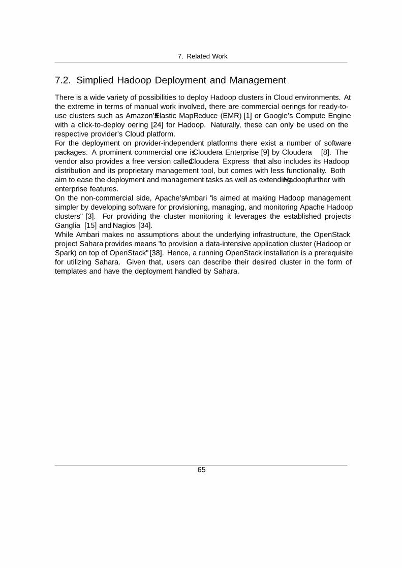
7. Related Work
7.2. Simplified Hadoop Deployment and Management
There is a wide variety of possibilities to deploy Hadoop clusters in Cloud environments. Atthe extreme in terms of manual work involved, there are commercial offerings for ready-to-use clusters such as Amazon’s Elastic MapReduce (EMR) [1] or Google’s Compute Enginewith a click-to-deploy offering [24] for Hadoop. Naturally, these can only be used on therespective provider’s Cloud platform.For the deployment on provider-independent platforms there exist a number of softwarepackages. A prominent commercial one is Cloudera Enterprise [9] by Cloudera [8]. Thevendor also provides a free version called Cloudera Express that also includes its Hadoopdistribution and its proprietary management tool, but comes with less functionality. Bothaim to ease the deployment and management tasks as well as extending Hadoop further withenterprise features.On the non-commercial side, Apache’s Ambari ”is aimed at making Hadoop managementsimpler by developing software for provisioning, managing, and monitoring Apache Hadoopclusters” [3]. For providing the cluster monitoring it leverages the established projectsGanglia [15] and Nagios [34].While Ambari makes no assumptions about the underlying infrastructure, the OpenStackproject Sahara provides means ”to provision a data-intensive application cluster (Hadoop orSpark) on top of OpenStack” [38]. Hence, a running OpenStack installation is a prerequisitefor utilizing Sahara. Given that, users can describe their desired cluster in the form oftemplates and have the deployment handled by Sahara.
65

8. Conclusion and Outlook
We have developed a Hadoop-based approach for automated deployment and distributedexecution of applications in Cloud environments with minimal effort on the user side. Animportant aspect of our work was to impose as few requirements as possible onto the setof potential applications that can be executed using our framework to design it as genericas possible. Besides Hadoop, we employed tools for the provisioning and configuration ofvirtual computing resources.
To evaluate our approach, we performed two case studies using applications developed byresearchers of the Software Engineering for Distributed Systems group of thisuniversity. Our interest besides investigating the effort needed to deploy and execute ap-plications using our solution was to measure the speedup gained in comparison to a non-distributed execution of the application, i.e. how much time the users can save from usingthe Cloud-based approach in relation to running the application on their local workingmachine. In both cases, our results showed that our approach is favourable. First, theapplications could be adapted easily to fit our modest requirements. Second, under mostscenarios we observed a speedup which was varying in size depending on the structure ofthe particular scenario.
Since our approach is based on Hadoop Streaming, which is a wrapper to execute arbi-trary applications using the MapReduce framework, a logical consequence was to compareour approach’s performance with that of a native MapReduce application to be able todraw qualified conclusions about either option’s advantages and disadvantages. Again, thespeedup was our primary criterion of interest. Moreover, we also documented the effortneeded to modify an existing application to employ MapReduce for its compute-intensivetasks. Naturally, due to the heterogeneity of software, it is only possible to examine thesequestions on a per-case basis. For the context of this thesis we chose one of our case studyapplications as the object of investigation.
Again, the results were in favour of our approach. Though the MapReduce version per-formed better than the reference situation,i.e. the non-distributed execution, and thus is animprovement in itself, our approach still outperformed it, though not by much. Also, thedevelopment work the user needs to invest is by far larger than to adapt the application toour requirements.
66

8. Conclusion and Outlook
Summarizing, the approach developed in the context of this thesis is an applicable solu-tion for automatically deploying and executing applications in Cloud environments withthe goal of reducing the overall execution time and without the user having to learn aboutCloud Computing internals.
8.1. Future Research Directions
Currently, there is a fixed one-file-one-task-mapping implying that each node processes ex-actly one file at a time. As we have seen in one of our case studies, it might be beneficial togive the user the possibility to influence this mapping while retaining the simplicity of theconfiguration. A basic solution may introduce an additional parameter in the job descrip-tion for specifying the files-per-task-mapping.
Further, the cluster size is currently set by the user prior to any job execution and thenremains constant. However, depending on the particular job it may be desirable to add orremove compute resources to either shorten the execution time or to save costs. While ourdeployment software is already prepared for scaling of the cluster, the required scaling logicis a topic for future research.Here, both a user-configurable and a machine learning-based approach is conceivable.
Throughout this thesis we used an OpenStack Cloud and our software is currently hard-coded to work with this IaaS platform. For use with other systems a Cloud-agnostic im-plementation would be necessary. Supporting other providers would only require modestchanges to our approach as long as there is a Vagrant plugin available for the desiredprovider.
Finally, we did not consider the issue of keeping the software on the cluster up-to-dateor security issues in general. Rather, we treat the clusters as just short-lived compute re-sources that are created and destroyed on-demand. For real-world application where securityconsiderations are warranted our approach needs to be extended in this direction.
67

A. Abbreviations and Acronyms
API Application Programming Interface
ASF Apache Software Foundation
AWS Amazon Web Services
DSL Domain-Specific Language
HDFS Hadoop Distributed File System
EMR Elastic MapReduce
GWDG Gesellschaft fur wissenschaftliche Datenverarbeitung Gottingen
HPC High Performance Computing
IaaS Infrastructure as a Service
IOPS Input/Output Operations Per Second
JSON JavaScript Object Notation
LOC Lines of Code
MPI Message Passing Interface
NFS Network File System
NFV Network Functions Virtualization
PaaS Platform as a Service
POSIX Portable Operating System Interface
RAID Redundant Array of Independent Disk
SaaS Software as a Service
SCM Software Configuration Management
68

A. Abbreviations and Acronyms
SIMD Single Instruction Multiple Data
STDIN Standard Input
STDOUT Standard Output
VM Virtual Machine
YARN Yet Another Resource Negotiator
69

B. Source Code Excerpts
B.1. Vagrantfile Template
Listing B.1: Vagrantfile Template for Cluster Provisioning
1 # −*− mode : ruby −*−2 # vi : s e t f t=ruby :34 # V a g r a n t f i l e template f o r c l u s t e r . py t o o l .5 # DO NOT EDIT UNLESS YOU KNOW WHAT YOU ARE DOING.67 VAGRANTFILE API VERSION = ”2”8 SLAVES COUNT = $count9
10 Vagrant . c o n f i g u r e (VAGRANTFILE API VERSION) do | c o n f i g |11 c o n f i g .vm. box = ’dummy’12 c o n f i g . ssh . username = ’ root ’13 c o n f i g . ssh . p r iva te key path = ’ $key path ’14 c o n f i g .vm. s y n c e d f o l d e r ’ . ’ , ’/ vagrant ’15 c o n f i g .vm. boot t imeout = 6001617 c o n f i g .vm. prov ide r : openstack do | os |18 os . opens tack auth ur l = ’ https : // api . c loud . gwdg . de :5000/ v2
.0/ tokens ’19 os . username = ’ $username ’20 os . password = ’ $password ’21 os . tenant name = ’ $tenant name ’22 os . f l a v o r = ’ $ f l avo r ’23 os . image = ’7 d9da5d4−2b56−477c−bb03−4
e731ad59f3e ’24 os . f l o a t i n g i p p o o l = ’ publ ic ’25 os . keypair name = ’ $key name ’26 end27
70

B. Source Code Excerpts
28 c o n f i g .vm. d e f i n e ”namenode ” do | namenode |29 namenode .vm. hostname = ”namenode ”30 end3132 SLAVES COUNT. t imes do | i |33 c o n f i g .vm. d e f i n e ” s l a v e#{ i +1}” do | s l a v e |34 s l a v e .vm. hostname = ”s l a v e#{ i +1}”35 end36 end3738 c o n f i g .vm. d e f i n e ”resourcemanager ” do | resourcemanager |39 resourcemanager .vm. hostname = ”resourcemanager ”4041 resourcemanager .vm. p r o v i s i o n : a n s i b l e do | a n s i b l e |42 a n s i b l e . verbose = ”v ”43 a n s i b l e . sudo = true44 a n s i b l e . playbook = ”$MTT HOME/ c l u s t e r /deployment/ s i t e .
yml ”45 a n s i b l e . l i m i t = ” a l l ”4647 s l a v e s = ( 1 . .SLAVES COUNT) . to a . map { | id | ”s l a v e#{id
}”}48 a n s i b l e . groups = {49 ”NameNode” => [ ”namenode ”] ,50 ”ResourceManager ” => [ ” resourcemanager ”] ,51 ”S laves ” => s l a v e s52 }53 end54 end55 end
71

B. Source Code Excerpts
B.2. cluster --project init Ansible Code
Listing B.2: Ansible Play Code for Project Initialization
1 −−−2 # Playbook f o r synchron i za t i on step in c l u s t e r −−p r o j e c t i n i t3 − hos t s : namenode4 remote user : root5 ta sk s :6 − name : Synchronize input data to NameNode7 synchron ize : s r c ={{ d i r path }} dest=/home/hadoop d e l e t e=yes
r e c u r s i v e=yes8 − name : Change ownership to Hadoop user9 s h e l l : chown −R hadoop : hadoop /home/hadoop/{{ dir name }}
1011 − hos t s : namenode12 remote user : root13 sudo : yes14 sudo user : hadoop15 ta sk s :16 − name : Import input data to HDFS17 s h e l l : cp −R /home/hadoop/{{ dir name }} /mnt/ hdfs / # TODO:
Move in s t ead o f copy
72

B. Source Code Excerpts
B.3. cluster --project destroy Ansible Code
Listing B.3: Ansible Play Code for Project Removal
1 −−−2 # Playbook f o r se rver−s i d e data removal in c l u s t e r −−
p r o j e c t d e s t r o y3 − hos t s : namenode4 remote user : root5 sudo : yes6 sudo user : hadoop7 ta sk s :8 − name : Remove d i r e c t o r y from HDFS9 s h e l l : rm −r f /mnt/ hdfs /{{ dir name }}
10 − name : Remove d i r e c t o r y from NameNode11 s h e l l : rm −r f /home/hadoop/{{ dir name }}
73

B. Source Code Excerpts
B.4. job --start Ansible Code
Listing B.4: Ansible Play Code for Job Execution
1 −−−2 # job −−s t a r t playbook34 − hos t s : namenode5 remote user : root6 ta sk s :7 − name : Synchronize input data to NameNode8 synchron ize : s r c ={{ pro j e c t pa th }} dest=/home/hadoop d e l e t e
=yes r e c u r s i v e=yes9 − name : Change ownership to Hadoop user
10 s h e l l : chown −R hadoop : hadoop /home/hadoop/{{ project name}}
11 − name : Make MapReduce mapper executab l e12 f i l e : path=/home/hadoop/{{ project name }}/ . j o b c o n f i g /{{
job }}/ mr job . py mode=”u+rwx ” owner=hadoop1314 − hos t s : namenode15 remote user : root16 sudo : yes17 sudo user : hadoop18 ta sk s :19 − name : Remove temporary f i l e s from HDFS20 s h e l l : rm −r f /mnt/ hdfs /{{ project name }}/ . j o b c o n f i g /mnt/
hdfs /{{ project name }}/ t r a n s i e n t /mnt/ hdfs /{{project name }}/ out
21 − name : Wait 3 seconds22 pause : seconds=323 − name : Import input data to HDFS24 s h e l l : cp −R /home/hadoop/{{ project name }}/ . j o b c o n f i g /
home/hadoop/{{ project name }}/ t r a n s i e n t /home/hadoop/{{project name }}/ out /mnt/ hdfs /{{ project name }}
2526 − hos t s : a l l27 remote user : root28 ta sk s :29 − name : Unmount temporary d i r e c t o r y (1/3)
74

B. Source Code Excerpts
30 mount : s r c=/tmp/ l o c a l j o b o u t name=/mnt/ hdfs /{{ project name}}/ out f s t y p e=bind s t a t e=unmounted
31 − name : Unmount temporary d i r e c t o r y (2/3)32 mount : s r c=/tmp/ l o c a l j o b o u t name=/mnt/ hdfs /{{ project name
}}/ out f s t y p e=bind s t a t e=unmounted33 − name : Unmount temporary d i r e c t o r y (3/3)34 mount : s r c=/tmp/ l o c a l j o b o u t name=/mnt/ hdfs /{{ project name
}}/ out f s t y p e=bind s t a t e=unmounted3536 − hos t s : namenode37 remote user : root38 sudo : yes39 sudo user : hadoop40 ta sk s :41 − name : Remove temporary output d i r e c t o r y42 s h e l l : rm −r f /mnt/ hdfs /mr tmp43 − name : Execute MapReduce task44 s h e l l : s c r e en −dmS mr job sh −c ”/ opt/hadoop/ bin /hadoop j a r /
opt/hadoop/ share /hadoop/ t o o l s / l i b /hadoop−streaming −*. j a r −Dmapreduce .map . cpu . vcore s=2 −input /{{ project name }}/ .
j o b c o n f i g /{{ job }}/ i n p u t l i s t . txt −output /mr tmp −mapper/mnt/ hdfs /{{ project name }}/ . j o b c o n f i g /{{ job }}/ mr job .
py −inputformat org . apache . hadoop . mapred . l i b .NLineInputFormat && touch /mnt/ hdfs /{{ project name }}/ .j o b c o n f i g / jobdone ; s l e e p 30”
75

B. Source Code Excerpts
B.5. SerializationHelper Class
Listing B.5: SerializationHelper Class (taken from [41])
1 package de . ugoe . cs . cpdp . mapreduce ;23 import org . apache . commons . i o . IOUt i l s ;45 import java . i o . * ;67 import org . apache . hadoop . i o . Writable ;89 pub l i c c l a s s S e r i a l i z a t i o n H e l p e r {
10 pub l i c s t a t i c byte [ ] s e r i a l i z e ( Writable wr i t ab l e ) throwsIOException {
11 ByteArrayOutputStream out = new ByteArrayOutputStream ( ) ;12 DataOutputStream dataOut = n u l l ;13 t ry {14 dataOut = new DataOutputStream ( out ) ;15 wr i t ab l e . wr i t e ( dataOut ) ;16 } catch ( Exception e ) {17 System . out . p r i n t l n ( e ) ;18 }19 f i n a l l y {20 IOUt i l s . c l o s e Q u i e t l y ( dataOut ) ;21 }22 return out . toByteArray ( ) ;23 }2425 pub l i c s t a t i c <T extends Writable> T asWritable ( byte [ ] bytes ,
Class<T> c l a z z )26 throws IOException {27 T r e s u l t = n u l l ;28 DataInputStream dataIn = n u l l ;29 t ry {30 r e s u l t = c l a z z . newInstance ( ) ;31 ByteArrayInputStream in = new ByteArrayInputStream (
bytes ) ;32 dataIn = new DataInputStream ( in ) ;33 r e s u l t . r e adF i e l d s ( dataIn ) ;
76

B. Source Code Excerpts
34 } catch ( I n s t a n t i a t i o nExce p t i o n e ) {35 // should not happen36 a s s e r t f a l s e ;37 } catch ( I l l e g a l A c c e s s E x c e p t i o n e ) {38 // should not happen39 a s s e r t f a l s e ;40 } f i n a l l y {41 IOUt i l s . c l o s e Q u i e t l y ( dataIn ) ;42 }43 return r e s u l t ;44 }45 }
77

B. Source Code Excerpts
B.6. WekaTraining Class
Listing B.6: WekaTraining Class
1 package de . ugoe . cs . cpdp . t r a i n i n g ;23 import java . i o . * ;4 import java . u t i l . Arrays ;5 import java . u t i l . L i s t ;6 import java . u t i l . l o gg ing . Leve l ;78 import org . apache . commons . i o . output . NullOutputStream ;9
10 import de . ugoe . cs . u t i l . c on so l e . Console ;11 import weka . core . In s tance s ;12 import weka . c l a s s i f i e r s . C l a s s i f i e r ;1314 import org . apache . hadoop . i o . Writable ;1516 /**17 * Programmatic WekaTraining18 *
19 * f i r s t parameter i s Tra iner Name .20 * second parameter i s c l a s s name21 *
22 * a l l subsequent parameters are c o n f i g u r a t i o n params ( f o r examplef o r t r e e s )
23 * Cross Va l ida t ion params always come l a s t and are prepended with−CVPARAM
24 *
25 * XML Conf i gura t i ons f o r Weka C l a s s i f i e r s :26 * <pre>27 * {@code28 * <!−− examples −−>29 * <t r a i n e r name=”WekaTraining ” param=”NaiveBayes weka . c l a s s i f i e r s
. bayes . NaiveBayes ” />30 * <t r a i n e r name=”WekaTraining ” param=”L o g i s t i c weka . c l a s s i f i e r s .
f u n c t i o n s . L o g i s t i c −R 1.0E−8 −M −1” />31 * }32 * </pre>
78

B. Source Code Excerpts
33 *
34 */35 pub l i c c l a s s WekaTraining extends WekaBaseTraining implements
ITra in ingStrategy , Writable {3637 @Override38 pub l i c void apply ( In s tance s t ra inda ta ) {39 PrintStream e r r S t r = System . e r r ;40 System . se tEr r (new PrintStream (new NullOutputStream
( ) ) ) ;41 try {42 i f ( c l a s s i f i e r == n u l l ) {43 Console . t r a c e l n ( Leve l .WARNING,
St r ing . format ( ” c l a s s i f i e r n u l l! ”) ) ;
44 }45 c l a s s i f i e r . b u i l d C l a s s i f i e r ( t r a inda ta ) ;46 } catch ( Exception e ) {47 throw new RuntimeException ( e ) ;48 } f i n a l l y {49 System . se tEr r ( e r r S t r ) ;50 }51 }5253 pub l i c void wr i t e ( DataOutput out ) throws IOException {54 ByteArrayOutputStream bo = new
ByteArrayOutputStream ( ) ;55 ObjectOutputStream so = new ObjectOutputStream ( bo )
;5657 // Write c l a s s i f i e r ( Ins tance o f C l a s s i f i e r )58 so . wr i teObject ( c l a s s i f i e r ) ;59 so . f l u s h ( ) ;60 byte [ ] b = bo . toByteArray ( ) ;61 i n t l ength = b . l ength ;62 out . w r i t e I n t ( l ength ) ;63 out . wr i t e (b) ;6465 // Write c l a s s i f i e r C l a s s N a m e / c l a s s i f i e r N a m e66 out . writeUTF ( c l a s s i f i e r C l a s s N a m e ) ;
79
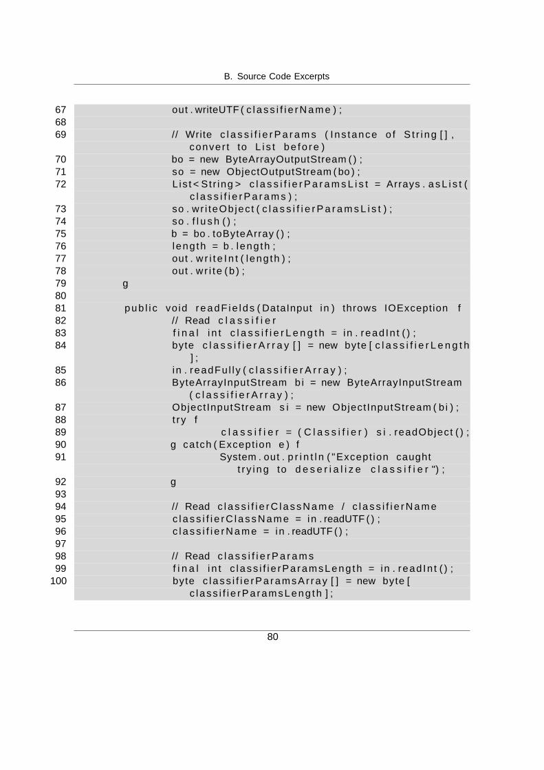
B. Source Code Excerpts
67 out . writeUTF ( c l a s s i f i e r N a m e ) ;6869 // Write c l a s s i f i e r P a r a m s ( Ins tance o f S t r ing [ ] ,
convert to L i s t be f o r e )70 bo = new ByteArrayOutputStream ( ) ;71 so = new ObjectOutputStream ( bo ) ;72 List<Str ing> c l a s s i f i e r P a r a m s L i s t = Arrays . a s L i s t (
c l a s s i f i e r P a r a m s ) ;73 so . wr i teObject ( c l a s s i f i e r P a r a m s L i s t ) ;74 so . f l u s h ( ) ;75 b = bo . toByteArray ( ) ;76 l ength = b . l ength ;77 out . w r i t e I n t ( l ength ) ;78 out . wr i t e (b) ;79 }8081 pub l i c void r eadF i e ld s ( DataInput in ) throws IOException {82 // Read c l a s s i f i e r83 f i n a l i n t c l a s s i f i e r L e n g t h = in . readInt ( ) ;84 byte c l a s s i f i e r A r r a y [ ] = new byte [ c l a s s i f i e r L e n g t h
] ;85 in . readFul ly ( c l a s s i f i e r A r r a y ) ;86 ByteArrayInputStream bi = new ByteArrayInputStream
( c l a s s i f i e r A r r a y ) ;87 ObjectInputStream s i = new ObjectInputStream ( bi ) ;88 try {89 c l a s s i f i e r = ( C l a s s i f i e r ) s i . readObject ( ) ;90 } catch ( Exception e ) {91 System . out . p r i n t l n ( ”Exception caught
t ry ing to d e s e r i a l i z e c l a s s i f i e r ”) ;92 }9394 // Read c l a s s i f i e r C l a s s N a m e / c l a s s i f i e r N a m e95 c l a s s i f i e r C l a s s N a m e = in . readUTF ( ) ;96 c l a s s i f i e r N a m e = in . readUTF ( ) ;9798 // Read c l a s s i f i e r P a r a m s99 f i n a l i n t c l a s s i f i e rParamsLeng th = in . readInt ( ) ;
100 byte c l a s s i f i e rPa ramsA r ray [ ] = new byte [c l a s s i f i e rParamsLeng th ] ;
80

B. Source Code Excerpts
101 in . readFul ly ( c l a s s i f i e rPa ramsAr ray ) ;102 b i = new ByteArrayInputStream (
c l a s s i f i e rPa ramsAr ray ) ;103 s i = new ObjectInputStream ( bi ) ;104 try {105 List<Str ing> c l a s s i f i e r P a r a m s L i s t = ( List<
Str ing >) s i . readObject ( ) ;106 c l a s s i f i e r P a r a m s = ( St r ing [ ] )
c l a s s i f i e r P a r a m s L i s t . toArray ( ) ;107 } catch ( Exception e ) {108 System . out . p r i n t l n ( ”Exception caught
t ry ing to d e s e r i a l i z e c l a s s i f i e r P a r a m s”) ;
109 }110 }111112 pub l i c s t a t i c WekaTraining read ( DataInput in ) throws
IOException {113 WekaTraining w = new WekaTraining ( ) ;114 w. r eadF i e ld s ( in ) ;115 re turn w;116 }117118 pub l i c S t r ing [ ] getParams ( ) {119 return c l a s s i f i e r P a r a m s ;120 }121 }
81
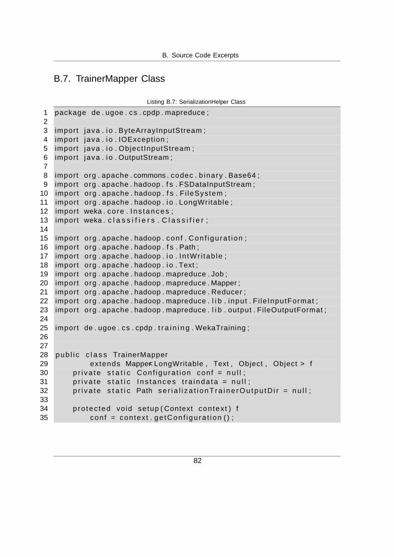
B. Source Code Excerpts
B.7. TrainerMapper Class
Listing B.7: SerializationHelper Class
1 package de . ugoe . cs . cpdp . mapreduce ;23 import java . i o . ByteArrayInputStream ;4 import java . i o . IOException ;5 import java . i o . ObjectInputStream ;6 import java . i o . OutputStream ;78 import org . apache . commons . codec . b inary . Base64 ;9 import org . apache . hadoop . f s . FSDataInputStream ;
10 import org . apache . hadoop . f s . Fi leSystem ;11 import org . apache . hadoop . i o . LongWritable ;12 import weka . core . In s tance s ;13 import weka . c l a s s i f i e r s . C l a s s i f i e r ;1415 import org . apache . hadoop . conf . Conf igurat ion ;16 import org . apache . hadoop . f s . Path ;17 import org . apache . hadoop . i o . IntWritab le ;18 import org . apache . hadoop . i o . Text ;19 import org . apache . hadoop . mapreduce . Job ;20 import org . apache . hadoop . mapreduce . Mapper ;21 import org . apache . hadoop . mapreduce . Reducer ;22 import org . apache . hadoop . mapreduce . l i b . input . Fi leInputFormat ;23 import org . apache . hadoop . mapreduce . l i b . output . FileOutputFormat ;2425 import de . ugoe . cs . cpdp . t r a i n i n g . WekaTraining ;262728 pub l i c c l a s s TrainerMapper29 extends Mapper<LongWritable , Text , Object , Object> {30 p r i v a t e s t a t i c Conf igurat ion conf = n u l l ;31 p r i v a t e s t a t i c In s tance s t ra inda ta = n u l l ;32 p r i v a t e s t a t i c Path s e r i a l i z a t i o n T r a i n e r O u t p u t D i r = n u l l ;3334 protec ted void setup ( Context context ) {35 conf = context . g e tCon f i gura t i on ( ) ;
82

B. Source Code Excerpts
36 s e r i a l i z a t i o n T r a i n e r O u t p u t D i r = new Path ( conf . get ( ”outputpath ”) ) ;
37 St r ing s e r i a l i z e d T r a i n d a t a = conf . get ( ” t ra inda ta ”) ;38 try {39 byte b [ ] = Base64 . decodeBase64 ( s e r i a l i z e d T r a i n d a t a ) ;40 ByteArrayInputStream bi = new ByteArrayInputStream (b) ;41 ObjectInputStream s i = new ObjectInputStream ( bi ) ;42 t ra inda ta = ( In s tance s ) s i . readObject ( ) ;43 } catch ( Exception e ) {44 System . out . p r i n t l n ( e ) ;45 }46 }4748 pub l i c void map( LongWritable key , Text value , Context context )49 throws IOException , Inter ruptedExcept ion {50 // Read s e r i a l i z e d t r a i n e r from HDFS51 Path i n p u t F i l e = new Path ( va lue . t oS t r i ng ( ) ) ;52 Fi leSystem f s = Fi leSystem . get ( conf ) ;53 FSDataInputStream in = f s . open ( i n p u t F i l e ) ;54 f i n a l i n t a v a i l a b l e = in . a v a i l a b l e ( ) ;55 byte s e r i a l i z e d T r a i n e r [ ] = new byte [ a v a i l a b l e ] ;56 in . readFul ly (0 , s e r i a l i z e d T r a i n e r ) ;5758 // D e s e r i a l i z e and apply t r a i n e r59 WekaTraining t r a i n e r = S e r i a l i z a t i o n H e l p e r . asWritable (
s e r i a l i z e d T r a i n e r , WekaTraining . c l a s s ) ;60 t r a i n e r . apply ( t ra inda ta ) ;6162 // S e r i a l i z e t r a i n e r and wr i t e to HDFS63 St r ing f i l ename = Long . t oS t r i ng ( System . nanoTime ( ) ) + ”. s e r
”;64 Path s e r i a l i z a t i o n F i l e = new Path (
s e r i a l i z a t i onTra ine rOutputD i r , f i l ename ) ;65 OutputStream os = f s . c r e a t e ( s e r i a l i z a t i o n F i l e ) ;66 os . wr i t e ( S e r i a l i z a t i o n H e l p e r . s e r i a l i z e ( t r a i n e r ) ) ;67 os . c l o s e ( ) ;68 }69 }
83

List of Figures
2.1. MapReduce Execution Phases [54] . . . . . . . . . . . . . . . . . . . . . . . . 132.2. HDFS Architecture [18] . . . . . . . . . . . . . . . . . . . . . . . . . . . . . . 152.3. YARN Architecture Overview [27] . . . . . . . . . . . . . . . . . . . . . . . . 17
3.1. Cluster Deployment Overview . . . . . . . . . . . . . . . . . . . . . . . . . . . 213.2. Virtual Machine Instantiation . . . . . . . . . . . . . . . . . . . . . . . . . . . 233.3. Virtual Machine Configuration . . . . . . . . . . . . . . . . . . . . . . . . . . 233.4. Job Management Overview . . . . . . . . . . . . . . . . . . . . . . . . . . . . 24
4.1. Architectural Overview . . . . . . . . . . . . . . . . . . . . . . . . . . . . . . 28
5.1. CrossPare Directory Structure . . . . . . . . . . . . . . . . . . . . . . . . . . . 45
6.1. WekaBaseTraining Class Diagram . . . . . . . . . . . . . . . . . . . . . . . . . 56
Listings
2.1. Vagrant Example . . . . . . . . . . . . . . . . . . . . . . . . . . . . . . . . . . 82.2. Ansible Example . . . . . . . . . . . . . . . . . . . . . . . . . . . . . . . . . . 112.3. MapReduce WordCount in Pseudo-code [54] . . . . . . . . . . . . . . . . . . . 122.4. Hadoop Streaming WordCount Example . . . . . . . . . . . . . . . . . . . . . 16
4.1. cluster config.json Example . . . . . . . . . . . . . . . . . . . . . . . . . . . . 304.2. user config.json Example . . . . . . . . . . . . . . . . . . . . . . . . . . . . . . 304.3. Vagrant Slave Instantiation . . . . . . . . . . . . . . . . . . . . . . . . . . . . 324.4. Setup of Vagrant/Ansible Interaction . . . . . . . . . . . . . . . . . . . . . . . 324.5. Job Description Example . . . . . . . . . . . . . . . . . . . . . . . . . . . . . 374.6. Server-side Job Execution . . . . . . . . . . . . . . . . . . . . . . . . . . . . . 39
84

4.7. Mapper Script . . . . . . . . . . . . . . . . . . . . . . . . . . . . . . . . . . . 394.8. Ansible File for Result Download . . . . . . . . . . . . . . . . . . . . . . . . . 41
5.1. Experiment Configuration (SMALL1) . . . . . . . . . . . . . . . . . . . . . . 455.2. TaskTreeCrossvalidation Configuration Example . . . . . . . . . . . . . . . . 49
6.1. Exemplary Loop from run() Method . . . . . . . . . . . . . . . . . . . . . . . 546.2. Serialization of Trainers . . . . . . . . . . . . . . . . . . . . . . . . . . . . . . 576.3. setup() Method of TrainerMapper . . . . . . . . . . . . . . . . . . . . . . . . 586.4. map() Method of TrainerMapper . . . . . . . . . . . . . . . . . . . . . . . . . 586.5. MapReduce Job Setup . . . . . . . . . . . . . . . . . . . . . . . . . . . . . . . 596.6. Trainer Deserialization . . . . . . . . . . . . . . . . . . . . . . . . . . . . . . . 60
B.1. Vagrantfile Template for Cluster Provisioning . . . . . . . . . . . . . . . . . . 70B.2. Ansible Play Code for Project Initialization . . . . . . . . . . . . . . . . . . . 72B.3. Ansible Play Code for Project Removal . . . . . . . . . . . . . . . . . . . . . 73B.4. Ansible Play Code for Job Execution . . . . . . . . . . . . . . . . . . . . . . . 74B.5. SerializationHelper Class (taken from [41]) . . . . . . . . . . . . . . . . . . . . 76B.6. WekaTraining Class . . . . . . . . . . . . . . . . . . . . . . . . . . . . . . . . 78B.7. SerializationHelper Class . . . . . . . . . . . . . . . . . . . . . . . . . . . . . . 82
List of Tables
2.1. Flynn’s Taxonomy . . . . . . . . . . . . . . . . . . . . . . . . . . . . . . . . . 4
3.1. User Credentials . . . . . . . . . . . . . . . . . . . . . . . . . . . . . . . . . . 223.2. Cluster Specification . . . . . . . . . . . . . . . . . . . . . . . . . . . . . . . . 223.3. Job Description Input . . . . . . . . . . . . . . . . . . . . . . . . . . . . . . . 25
4.1. Ansible Roles for Cluster Deployment . . . . . . . . . . . . . . . . . . . . . . 334.2. Services running on different Node Types . . . . . . . . . . . . . . . . . . . . 34
5.1. Hadoop Flavour . . . . . . . . . . . . . . . . . . . . . . . . . . . . . . . . . . . 425.2. Environment Software Versions . . . . . . . . . . . . . . . . . . . . . . . . . . 435.3. CrossPare Results . . . . . . . . . . . . . . . . . . . . . . . . . . . . . . . . . 475.4. TaskTreeCrossvalidation Results . . . . . . . . . . . . . . . . . . . . . . . . . 50
85

List of Tables
6.1. Streaming vs. MapReduce . . . . . . . . . . . . . . . . . . . . . . . . . . . . . 626.2. Local vs. MapReduce . . . . . . . . . . . . . . . . . . . . . . . . . . . . . . . 63
86

Bibliography
[1] Amazon Elastic MapReduce. Online: http://aws.amazon.com/de/elasticmapreduce/.Accessed: 2015-04-15.
[2] Ansible is Simple IT Automation. Online: http://www.ansible.com/home. Accessed:2015-04-15.
[3] Apache Ambari. Online: https://ambari.apache.org/. Accessed: 2015-04-15.
[4] Apache Commons. Online: http://commons.apache.org/. Accessed: 2015-04-15.
[5] AppScale. Online: http://www.appscale.com/. Accessed: 2015-04-15.
[6] AutoQUEST. Online: https://autoquest.informatik.uni-goettingen.de. Accessed:2015-04-15.
[7] Chef - Code Can. Online: https://www.chef.io/. Accessed: 2015-04-15.
[8] Cloudera. Online: http://www.cloudera.com/. Accessed: 2015-04-15.
[9] Cloudera Enterprise. Online: http://www.cloudera.com/content/cloudera/en/products-and-services/cloudera-enterprise.html. Accessed: 2015-04-15.
[10] Cloudera Express. Online: http://www.cloudera.com/content/cloudera/en/products-and-services/cloudera-express.html. Accessed: 2015-04-15.
[11] cloudinit.d. Online: http://www.nimbusproject.org/doc/cloudinitd/latest/. Accessed:2015-04-15.
[12] coreutils - GNU Core Utilities. Online: http://www.gnu.org/software/coreutils/.Accessed: 2015-04-15.
[13] Crosspare Application. Online: https://crosspare.informatik.uni-goettingen.de/svn/crosspare/trunk/CrossPare/. Accessed: 2015-04-15.
[14] ETSI - Network Functions Virtualisation. Online: http://www.etsi.org/technologies-clusters/technologies/nfv. Accessed: 2015-04-15.
[15] Ganglia. Online: http://ganglia.sourceforge.net/. Accessed: 2015-04-15.
87

Bibliography
[16] Google App Engine. Online: https://cloud.google.com/appengine. Accessed: 2015-04-15.
[17] Hadoop. Online: http://hadoop.apache.org/. Accessed: 2015-04-15.
[18] Hadoop. HDFS Architecture. Online: http://hadoop.apache.org/docs/r2.6.0/hadoop-project-dist/hadoop-hdfs/HdfsDesign.html. Accessed: 2015-04-15.
[19] Hadoop Mailing List - Why not use Serializable? Online: http://www.mail-archive.com/[email protected]/msg00378.html. Accessed: 2015-04-15.
[20] Hadoop Main 2.6.0 API - NLineInputFormat Class. Online:https://hadoop.apache.org/docs/stable/api/org/apache/hadoop/mapred/lib/NLineInputFormat.html.Accessed: 2015-04-15.
[21] Hadoop Main 2.6.0 API - Writable Interface. Online:https://hadoop.apache.org/docs/current/api/org/apache/hadoop/io/Writable.html.Accessed: 2015-04-15.
[22] Hadoop. MapReduce. Online: http://wiki.apache.org/hadoop/HadoopMapReduce.Accessed: 2015-04-15.
[23] Hadoop MapReduce tutorial. Online:http://hadoop.apache.org/docs/current/hadoop-mapreduce-client/hadoop-mapreduce-client-core/MapReduceTutorial.html. Accessed: 2015-04-15.
[24] Hadoop on the Google Cloud Platform. Online:https://cloud.google.com/solutions/hadoop/. Accessed: 2015-04-15.
[25] Hadoop. What is the Purpose of the Secondary Name-node? Online:http://wiki.apache.org/hadoop/FAQ#What is the purpose of the secondary name-node.3F. Accessed: 2015-04-15.
[26] Hadoop Wiki - How Many Maps And Reduces. Online:http://wiki.apache.org/hadoop/HowManyMapsAndReduces. Accessed: 2015-04-15.
[27] Hadoop. YARN. Online: http://hadoop.apache.org/docs/stable/hadoop-yarn/hadoop-yarn-site/YARN.html. Accessed: 2015-04-15.
[28] HashiCorp. Online: https://hashicorp.com/. Accessed: 2015-04-15.
[29] Java Documentation - Serializable Objects. Online:http://docs.oracle.com/javase/tutorial/jndi/objects/serial.html. Accessed:2015-04-15.
88

Bibliography
[30] Java Platform SE7 - Serializable Interface. Online:http://docs.oracle.com/javase/7/docs/api/java/io/Serializable.html. Accessed:2015-04-15.
[31] JavaScript Object Notation. Online: http://json.org/. Accessed: 2015-04-15.
[32] Meet Infrastructure as Code- DevOps.com. Online: http://devops.com/blogs/meet-infrastructure-code/. Accessed: 2015-04-15.
[33] Message Passing Interface (MPI). Online:http://www.mcs.anl.gov/research/projects/mpi/. Accessed: 2015-04-15.
[34] Nagios. Online: http://www.nagios.org. Accessed: 2015-04-15.
[35] Nimbus Project. Online: http://www.nimbusproject.org/. Accessed: 2015-04-15.
[36] OpenMP. Online: http://openmp.org/. Accessed: 2015-04-15.
[37] OpenStack. Online: http://www.openstack.org/. Accessed 2014-09-26.
[38] OpenStack Sahara. Online: https://wiki.openstack.org/wiki/Sahara. Accessed: 2015-04-15.
[39] Puppet Labs: IT Automation Software for System Administrators. Online:http://puppetlabs.com/. Accessed: 2015-04-15.
[40] Ruby Programming Language. Online: https://www.ruby-lang.org/. Accessed: 2015-04-15.
[41] Stack Overflow - How To Unit Test Hadoop Writable. Online:http://stackoverflow.com/questions/13288214/how-to-unit-test-hadoop-writable.Accessed: 2015-04-15.
[42] Tera-Promise Repository. Online: http://openscience.us/repo/. Accessed: 2015-04-15.
[43] TOP 500 Supercomputer Sites - Statistics. Online:http://www.top500.org/statistics/. Accessed: 2015-04-15.
[44] TORQUE Resource Manager. Online:http://www.adaptivecomputing.com/products/open-source/torque/. Accessed:2015-04-15.
[45] Vagrant. Online: https://www.vagrantup.com/. Accessed: 2015-04-15.
89

Bibliography
[46] Vagrant OpenStack Cloud Provider. Online: https://github.com/ggiamarchi/vagrant-openstack-provider. Accessed: 2015-04-15.
[47] Weka 3 - Data Mining with Open Source Machine Learning Software in Java. Online:http://www.cs.waikato.ac.nz/ml/weka/. Accessed: 2015-04-15.
[48] What is DevOps? Online: http://radar.oreilly.com/2012/06/what-is-devops.html.Accessed: 2015-04-15.
[49] YAML Specification. Online: http://www.yaml.org/spec/. Accessed: 2015-04-15.
[50] G. S. Almasi and A. Gottlieb. Highly Parallel Computing. Benjamin-CummingsPublishing Co., Inc., Redwood City, CA, USA, 1989.
[51] M. Armbrust, A. Fox, R. Griffith, et al. Above the Clouds: A Berkeley View of CloudComputing. Technical Report UCB/EECS-2009-28, University of California at Berke-ley, February 2009.
[52] C. Boyd. Data-parallel computing. Queue, 6(2):30–39, 2008.
[53] C. Bunch, N. Chohan, C. Krintz, and K. Shams. Neptune: a domain specific lan-guage for deploying hpc software on cloud platforms. In Proceedings of the 2nd inter-national workshop on Scientific cloud computing, pages 59–68. ACM, 2011.
[54] J. Dean and S. Ghemawat. MapReduce: Simplified Data Processing on Large Clus-ters. Commun. ACM, 51(1):107–113, January 2008.
[55] M. Flynn. Some Computer Organizations and Their Effectiveness. Computers, IEEETransactions on, C-21(9):948–960, Sept 1972.
[56] P. Harms and J. Grabowski. Usage-Based Automatic Detection of Usability Smells.In Human-Centered Software Engineering, pages 217–234. Springer, 2014.
[57] P. Harms, S. Herbold, and J. Grabowski. Trace-based task tree generation. In ACHI2014, The Seventh International Conference on Advances in Computer-Human Inter-actions, pages 337–342, 2014.
[58] J. L. Hennessy and D. A. Patterson. Computer Architecture, Fifth Edition: A Quan-titative Approach. Morgan Kaufmann Publishers Inc., San Francisco, CA, USA, 5thedition, 2011.
[59] S. Nanda and T. Chiueh. A Survey on Virtualization Technologies. Technical ReportTR-179, Stony Brook University, February 2005.
90

Bibliography
[60] National Institute of Standards and Technology. The NIST Definition of Cloud Com-puting. NIST Special Publication, (800-145), 2011.
[61] P. Pacheco. An Introduction to Parallel Programming. Morgan Kaufmann PublishersInc., San Francisco, CA, USA, 1st edition, 2011.
[62] S. Wadkar, M. Siddalingaiah, and J. Venner. Pro Apache Hadoop. Apress, Berkely,CA, USA, 2nd edition, 2014.
91

![Virtual Machine Provisioning Based on Analytical ...gridbus.csse.unimelb.edu.au/~raj/papers/VMProvisionCloud-ICPP201… · Cloud Provisioning [3] is the process of deployment and](https://img.pdfslide.net/doc/110x75/5ed5c6a808214b19be6a1da7/virtual-machine-provisioning-based-on-analytical-rajpapersvmprovisioncloud-icpp201.jpg)