LA-6885-MSInformal Report UC-32GIC-74 REPORT COLLECTION

REPRODUCTION Issued: July 1977

copy

Automated Heuristic Stability Analysis for

Nonlinear Equations

L. D. CIoutman

L. W. Fullerton

t

).

J’Ialamos

scientific laboratoryof the university of California

LOS ALA MOS, NEW MEXICO 87545

An Affirmative Action /Equcrl Opportunity Employer

uNITED STATES

ENERGY RESEARCH AND DEVELOPMENT ADMINISTRATION

CONTRACT W-7405 -ENG. 36

PrintedintheUnitedStatesofAmerica.AvailablefromNationalTechnicalInformationService

U.S.DepartmentofCommerce5285PortRoyalRoadSprirrgtleld,VA 22161

Price:PrintedCopY $4.50Microfiche$3.00

Thi. rewrt w.. pmp.r.d . . . . .cc...1 .[ work .vons.mdb. the [,nimd St.te. (:o..rnmcnt. Xeilher the l!nited SIat.snor the t%iwd SI.trs Kncrm Rrsc.rch and Ik.vcl.pm.nt Ad.mi. i.tr.t i... nor ●n, .( !heir .IIIPI.Y.CS, nor ..} of their . . . .trm’tor.. Sublwntr”c’to,.. or :hoir ●mpl., ees. m.kes myw..rr.ml>..xp....0. ,mplicd... ..wIII.-...v 11-K.IIi.hil it. orrqwmihilitv (W th. xc. ra.t. .ompl.t.n.sh or u.efulnrs. of.nv inform. ti,, n. .IUU..l . . . product. or proce.. dkclo.rd. ortcpr.., ot. th.t il. .u- would not in frinae Privat.h ownedright.

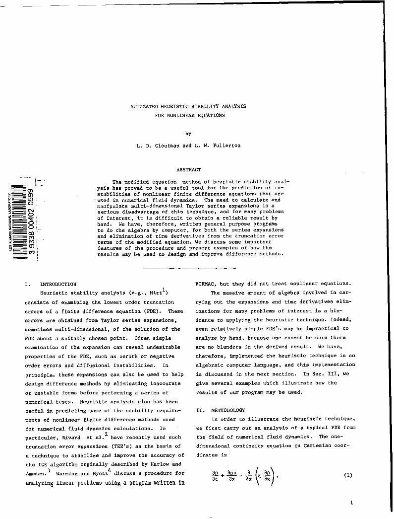
AUTOMATED HEURISTIC STASILITY ANALYSIS

FOR NONLINEAR EQUATIONS

by

L. D. Cloutman and L. V. Fullerton

AESTRACT

_ 1=The modified equation method of heuristic stability anal-

-m” ysis has proved to be a useful tool for the prediction of in->~ a stabilities of nonlinear finite difference equations that are~sm:s0. -

-used in numerical fluid dynamics. The need to calculate and

:~gmanipulate multi–dimensional Taylor series expansions is a

~co:serious disadvantage of this technique, and for many problems

d-’ of interest, it ia difficult to obtain a reliable result by

Szo ~. hand. We have, therefore, written general purpose programs

-a~~ to do the algebra by computer, for both the series expansions

3=%qnd elimination of time derivatives from the truncation error

~~m\terms of the modified equation. We discuss some important

~~~features of the procedure and present examplea of how the

—! results may be used to design and improve difference methods.

I. lNTRODUCT1ON

‘deuriaticstability analysis (e.g., ‘dirtl)

consists of examining the lowest order truncation

errors of a finite difference equation (FDE). These

errors are obtained from Taylor series expansions,

sometimes multi-dimensional, of the solution of the

FDE about a suitably chosen point. Often simple

examination of the expansion can reveal undesirable

properties of the FDE, such as zeroth or negative

order errors and diffusional instabilities. In

principle, these expansions can also be used to help

design difference methods by eliminating inaccurate

or unstable forms before performing a series of

numerical tests. Heuristic analysis also has been

useful in predicting some of the stability require-

ments of nonlinear finite difference methods used

for numerical fluid dynamics calculations. In2

particular, Rivard et al. have recently used such

truncation error expansions (TEE’s) as the basis of

a technique to stabilize and improve the accuracy of

the ICE algorithm orginally described by Harlow and

Amsden.3 Warming and Hyett4 discuss a procedure for

analyzing linear problemg using a program written in

FORNAC, but they did not treat nonlinear equations.

The maasive amount of algebra involved in car–

rying out the expansions and time derivatives elim-

inations for many problems of interest ia a hin-

drance to applying the heuristic technique. Indeed,

even relatively simple FDE’s may be impractical to

analyze by hand, because one cannot be sure there

are no blunders in the derived result. We have,

therefore, implemented the heuristic technique in an

algebraic computer language, and this implementation

is discuaaed in the next section. In Sec. III, we

give several examples which illustrate how the

results of our program may be used.

II. METHODOLOGY

In order to illustrate the heuristic technique,

we first carry out an analysis of a typical FDE from

the field of numerical fiuid dynamica. The one-

dimenaional continuity equation in Cartesian coor-

dinates is

(1)

1

where p is the fluid density, u is the velocity,and

~ is an artificial mass diffusion coefficient that

may be needed for stability. For the ICE method,

we approximate Eq. (1) by

1+p:) U;* - (p: + P:_l) u;_%

we substitute Eq. (3) for each of the variables in

Eq. (2) and drop high-order terms, we obtain the

original differential equation plus extra terms that

we call truncation er~ors:

+

[‘> Ci-%+(pY+l - P;) - ei_%(P;

+

- P:_l)j ,

(2)

where a superscript denotea the time level and a

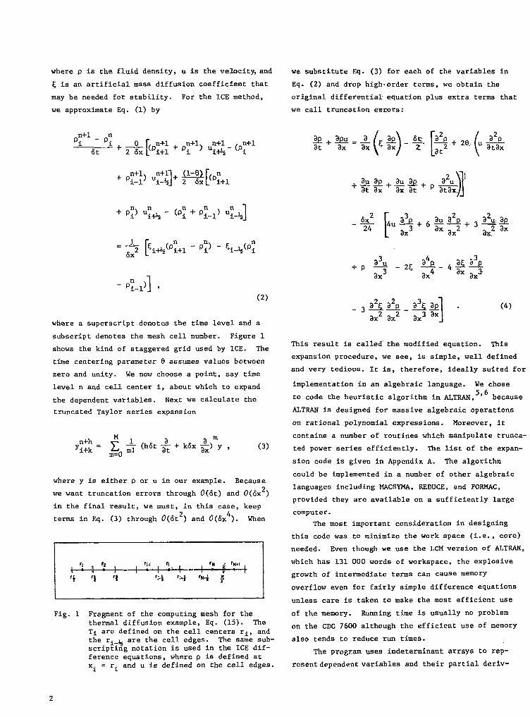
subscript denotes the mesh cell number. Figure 1

shows the kind of staggered grid used by ICE. The

time centering parameter .9assumes values between

zero and unity. We now choose a point, say time

level n and cell center i, about which to expand

the dependent variables. Next we calculate the

truncated Taylor series expansion

where y is either p

(h6t;+ k6x#Jmy , (3)

or u in our example. Because

we want truncation errors through ()(6t)and 0(6x2)

in the final result, we must, in this case, keep

terms inEq. (3) through 0(&t2) and 0(6x4). When

[

Fig. 1 Fragment of the computing mesh for thethermal diffusion example, Eq. (15). TheTi are defined on the cell centers ri, andthe ri_% are the cell edges. The same sub-scripting notation is used in the ICE dif-ference equations, where p is defined atxi=r i and u is defined on the cell edges.

%(d@-[$+2e(u&

1./

au ap + &s+p&—.at ax ax at

~24

[

4u&+6~&+3?&%

ax3 ax2 ~x2 ax

p#u-a4

a~ 83Q2C +-4axax3

ax3 ax

1

3&&_&% . (4)

ax2 ax2 3X3 ax

This result is called the modified equation. This

expansion procedure, we see, is simple, well defined

and very tedious. It is, therefore, ideally suited for

implementation in an algebraic language. We chose5,6to code the heuristic algorithm in ALTRAN, because

ALTRAN is designed for massive algebraic operations

on rational polynomial expressions. Moreover, it

contains a number of routines which manipulate trunca-

ted power series efficiently. The list of the expan-

sion code is given in Appendix A. The algorithm

could be implemented in a number of other algebraic

languages including MACSYMA, REDUCE, and FORMAC,

provided they are available on a sufficiently large

computer.

The most important consideration in designing

this code waa to minimize the work space (i.e., core)

needed. Even though we use the LCM version of ALTRAN,

which has 131 000 words of workspace, the explosive

growth of intermediate terms can cause memorY

overflow even for fairly simple difference equations

unless care is taken to make the most efficient use

of the memory. Running time is usually no problem

on the CDC 7600 although the efficient use of memory

also tends to reduce run times.

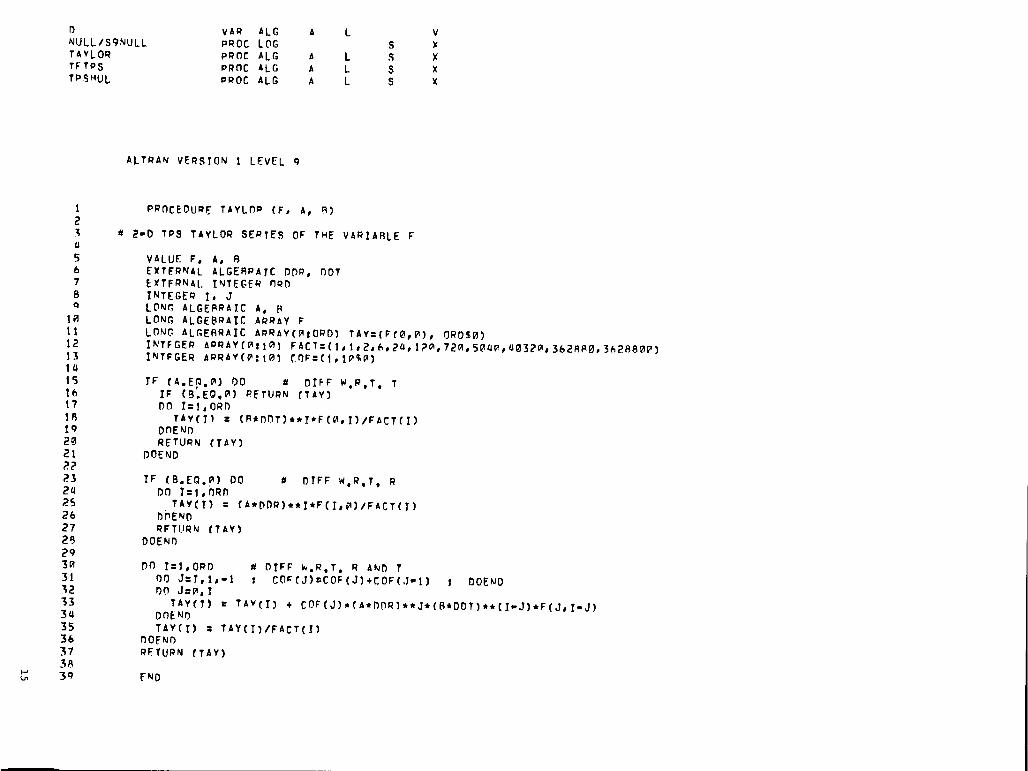
The program uses indeterminant arrays to rep-

resentdependentvariables and their partial deriv-

(i+j) ~/axiatj is representedatives. For example, 3

by the array element U(I,J). The code is set up to

handle four such variables; P, T, RHO, and U. More

variables can be added to the layout if needed,

although they would increase memory requirements.

The maximum order of the expansions is set by the

integer variable ORD, currently set to a value of

six. The maximum value of I or J is set by the

integer variable N, also currently set equal to six.

If higher order derivatives or expansions are needed

st any point in the calculation, N and/or ORD must be

increased, with a corresponding increase in memory

requirements and running time. In practice, however,

even large, high-order problems are practical on the

l.ASL7600’s,

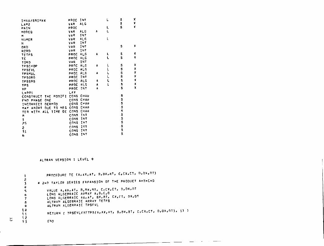
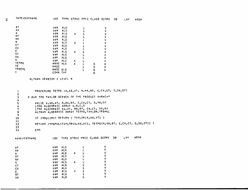
The Taylor series expansions are done by the

LONG ALGEBRAIC ALTRAN PROCEDURE TE, which is invoked

as a function. Suppose we choose (i &r, n fit)

as the point about which we want to perform the

expansions. A single call to TE csn expand a prod-

uct of up to four variables. The calling sequence

TE(fl,al, b f a b f a b f a b)expands1* 29 29 29 3* 3* 39 49 49 4

(fl)‘+bl (f2)n+b2 (f3)*+b3 (f4)n+b4 to order ORD ini-l-a

1i+a

2 i+a3

i+a4

both &r and &t. For example,n+l

is represented by‘i-%

TE(u,-1/2,1). It is more efficient to compute prod-

ucts with a single call than to make separate calls

and multiply the results. That is, usen+l nTE(RHO, O, 1, U, 1/2, O) for pi ui~, not

TE(RHO, O, 1)* TE(U, 1/2, O). The first method com-

putes only terms of order ORD. The latter method

expands each variable to order OW, and the mul-

tiplication generatee many terms through order 2*ORD

that are eventually discarded.

Since there is no simple way to specify the dif-

ference equation on data cards, all input data Is

specified in executable ALTRAN statements in a spe-

cial section of the program. RORD and TORD are the

maximum orders of &r and &t,respectively,to be

retained in the final result. DERMOD is the left-

hand side of the modified equation, and it will be

explained in more detail in the example. DE is the

differential equation, and FDE is the finite dif–

ference equation expressed in terms of ill?.lhe

listing of the code in Appendix A contains Eq.

(2) as an example. Note that DE and FDE are always

written in the fonu such that they are equal to zero.

we want the truncation errors to ~(6t) and 0(6r2),

so RORD = 2 and TORD = 1. Since the expansions are

divided by 6t and &2, they must be carried out to

at least order 2 and 4 in 6t and & respectively.

Therefore, ORD must be at least 4.

T%ia example is a trivial problem -- only 14

seconds of central processor time and 37 000 words

of workspace were required on a CDC 7600. Although

131 000 words of workspace are available in our

version of ALTRAN, memory space, not running time,

still Mmits the size of the largest problem that

can be run. Very large problems often can be run

piecemeal, however.

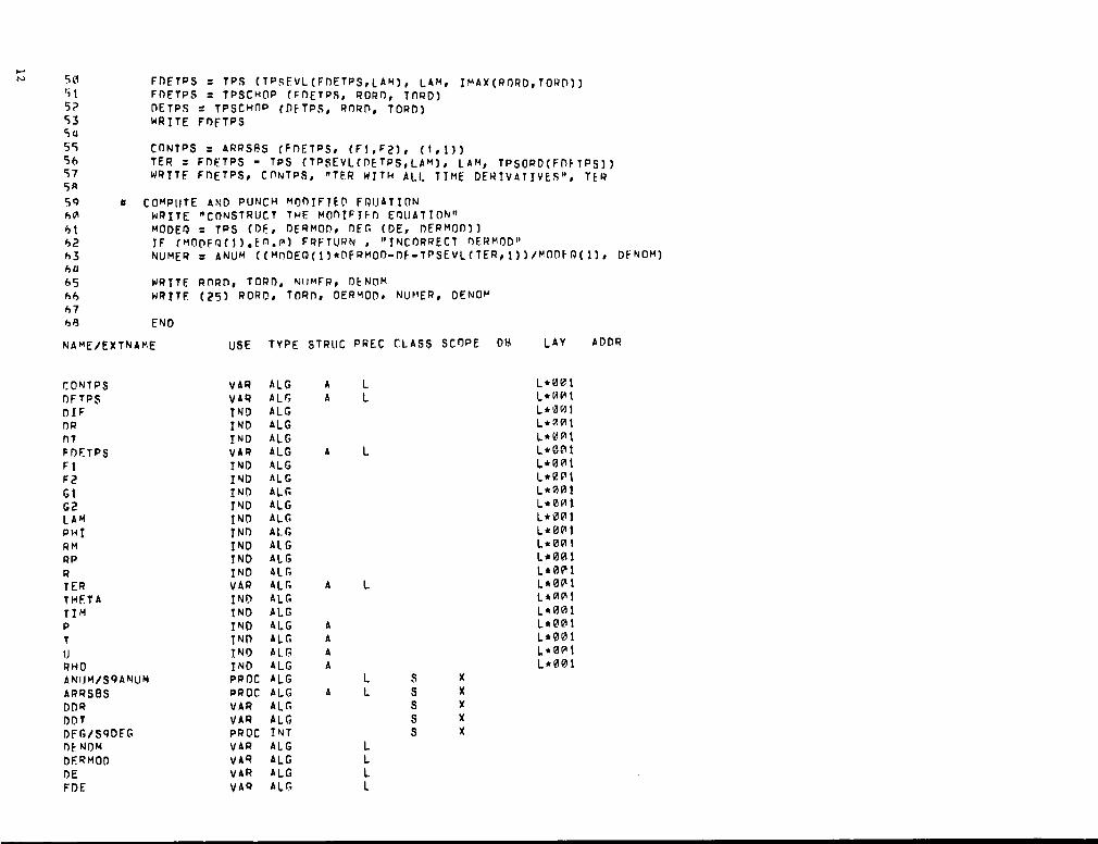
Appendix A consists of a complete listing of

the expansion code, plus a sample problem. Appendix

B contains a detailed flow chart of the ALTRAN cod-

ing, definition of all variables, and a description

of the purpose and operation of every procedure.

For some purpose it is necessary to eliminate

all time derivatives from the modified equation.

In our example, we need ap/2t and 2MIM and their

derivatives with respect to both r and t. Therefore,

the modified equation is punched out in the form

DERMOD= RHO(O,l) =~=–~- p%+ &ax

(5)

The time derivative elimination code then differen-

tiates the right-hand side and eliminates the time

derivative from the truncation error terms TER.

It is necessary to use the modified equation for the

momentum equation to eliminate the time derivatives

of u. We will return this example in the next sec-

tion.

A simpler example will suffice to illustrate

the complexities of automating the general procedure

for eliminating time derivatives. The modified

equation for the difference approximation,

n+1Ti - T; ~

&t “~(

FnnL-I-1)

- 2Ti + ‘i-1

to

aT .Kfi,Ft

ax2

(6)

(7)

3

expanded about time n and space point i is

aT2 2

6X2K a4T—=K~–~~+~ —at + o(6t2,6x4).

ax at ax4(8)

We will keep error terms of order 6t and 6X2. Begin

the elimination of a2T/M2 by differentiating Eq.

(8) wf,threspect to t,

fit Z13T+&.K 23T —— 6X2K a5T

at2 ax2at 2 at3 6 ax4at

Substitute Eq. (9) into Eq. (8) and discard

der terms:

g = ~ E12T 6tK 23T + dX2K 24Tat .

ax2 2 ax2at 6 ax4

Note

tive

iate

that we have lowered the order of time

in the error terms by one. Now we can

Eq. (8) with respect to x to obtain

a3T = K a4T dt a4T + 6X2K a6T

ax2at ax4 2 ax2at2 6~x6 ‘

which we substitute into Eq. (10):

w=K&+_

()

K6x2 1 K& a4T._—at

ax2 2 3 6X2~“

(9)

high-or-

(10)

deriva-

differen-

(11)

(12)

It is obvious from this trivial example that the

elimination of time derivativea from the truncation

error terms of the modifed equation is,in general,a

very messy algebraic problem for the general case of

coupled nonlinear partial differential equations.

The code and flow charta listed in Appendixes C and

D describe a first attempt to solve this problem.

Although this program is capable of handling very

large problems in a reasonable amount of central

processor time, a clever programmer should be able

to improve its efficiency. For this and other rea-

sons to be discussed later, this code should be

considered a useable but unpolished tool.

The elimination code reads its input from cards

punched either by itself or

elimination code only makes

4

the expansion

a single pass

code. The

at elim-

inating the time derivatives, lowering the order of

the time derivatives by at most one per run. Thus,

our simple example would require two runs. The

first run would read carde punched by the expansfon

code, and the next run (and all subsequent runs if

necessary) would read the cards punched by the expan-

sion code on the previous run. This multiple run

procedure is inefficient in terms of the human inter-

vention and turn around time involved, and we intend

to eventually combine the expansion and elimination

codes into a single completely automated code.

The elimination code can aleo handle simple

systems of equations. It can read a second modified

equation and substitute derivatives of the first, or

primary, modified equation into the second, or sec-

ondary, modified equation. Our limited experience

with systems of modified equations suggests that

improving the efficiency of workspace utilization

should receive high priority in the list of improve-

ments to this code. The memory problem is not se-

rious with the LCM version of ALTRAN available on

the CROS operating system, where 131 000 decimal

words of workspace are available, but it is likely

to be quite limiting at installations with smaller

workspaces. Some steps for reducing memory require-

ments and the mmber of runs are described in Appen-

dix C.

III. APPLICATIONS

Truncation error expansions may be employed in

three ways. First, they indicate the order and ac-

curacy of FDE’s, and so they may be used to help

choose the beat form for a particular problem. Sec-

ond, they may be used to find stability conditions

for some problems. And finally, they may be employed

as the basis of a new method for stabilizing some

finite difference algorithms. In this section we

discuss examples of each of these applications. We

emphasize that although most of our examples are

relatively simple and could be done by hand, the

ALTRAN programs are powerful tools that can do and

have done expansions much too large and complicated

to do reliably by hand in a reasonable amount of

time.

a. Comparison of Errors of Difference Equations

The TEE’s easily indicate some undesirable

properties of FDE’s, such as zeroth-or negative-

order errors. Such information is quite useful,

for it may rule out use of a particular FDE before

it is coded and subjected to numerical tests. But

beyond such simple observations, FDE’s are not easily

compared. The next example illustrates the type of

analysis frequently necessary to determine which one

of several FDE’s is more accurate. Consider the one-

dimensional diffusion problem in spherical coordinates

(13)

T(r,O) =* ,

T(n,t) = O ,

and

~ (O,t) = o ,

where $ is a constant. The analytic solution is

T(r,t) = exp(-$t) sin(r)/r . (14)

Now consider the explicit FDE

,p+l_ ,f

—-J=++!-_i

[

r2i+%(’;+l - ‘~)

&t r.-ri 1+1 1

r~_%(T~ - T~_l)

r. - r.1 1-1 1 (15)

The computing mesh is illustrated in Fig. 1. We

compare the accuracy of two different definitions of

Vi in Eq. (15):

Vi = (r~q+- r~_%)/3 (16a)

and

Vi ‘ r: (ri%- ‘i_~) . (16b)

Note that the cells are spherical shells, and Vi is

the volume of one steradian of the ith cell.

Heuristically we expect Eq. (16a) to be more

accurate than Eq. (16b) near the origin, because the

former volume elements exactly fill space. The lat-

ter volume elements are all smaller than the former

for the same set of mesh

most pronounced at small

give conservative FDE’s,

amOunts of the conserved

points, and the effect is

r. Both volume elements

but they conserve different

quantity. For constant T,

volume elements in Eq. (16a) lead to conservation of

the correct amount of the conserved quantity

fi1247

IT r2dr, but Eq. (16b) conserves the wrong

0

amount.

We can use the expansions to determine which

volume element is more accurate. The TEE’s for Eq.

(15) with Eqs. (16a) and (16b), respectively, are

equivalent to

-[+-+k$++l‘~ [$-4 ‘o(’t2’r4)

(17a)

and

1+ 4 213T +4 6r2 a2T— . + 0(rSt2,6r4) (17b)r &3 4 r2 2r2

for a uniform mesh.

At first glance, Eq. (17b) appears better than

Eq. (17a) because the coefficient of ~ in Eq. (17a)

is proportional to l/r3. Furthermore, unlike Eq.

(16a), Eq. (16b) leads to a difference scheme which

is exact for a solution T, linear in r. Thus, our

earlier arguments about volume elements in Eq. (16a)

being better appear to be wrong. However, as we

shall show, our superficial examination of Eqs. (17a)

and (17b) is at fault.

Currently, there is no general procedure for

5

choosing the more accurate of several FDE’s,based on

Taylor series expansions. But we now present a

procedure which works many problems, and we hope it

will provide a basis for an even more general proce-

dure. The cursory examination above is misleading,

because ~ = O at the origin and because some error

terms partially cancel each other. We expand T in

Taylor series about r = O for some II,O < ~ < r5,2,

andatimeT, tn<?< t’n+l”

(21a)‘N+l= ‘TN + 2Tb

or

1 8‘N+l = ‘2TN+~TN-l ‘~Tb’

(21b)

For boundary

respectively, th

where Tb = O is the boundary value.

conditions in Eqs. (21a) and (21b),

right side of Eq. (15) is equivalent to~ 21(i)T(0,T)~ .

T(rl,T) =i=o ar(i) i!

(18)

After differentiating Eq. (18) and substituting into

the space errors of Eqs. (17a) and (17b), we find(22a)

Each equation is valid for both volume elements in E

(16a) and (16b). Note that the simpler Eq. (21a) ha

a large zeroth-order in the diffusion term. Therefo

we expect the first-order boundary conditions in Eq.

(21b) to be more accurate in the outer part of the

mesh where the boundary treatment dominates the

accuracy of the solution.

1+O(rlo) (19a)

and

In order to substantiate our deductions based

[

& &T+4a3T+++12 ar4

r ar3 r ,% 1r=qon TEE’s, we numerically solved Eq. (15) using Sev-

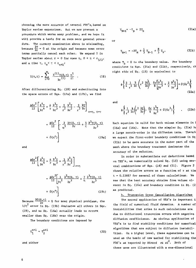
eral combinations of Eqs. (16) and (21). Figure 2

shows the relative errors as a function of r at time

t = 0.23687 for several of these calculations. We

[

_ @r2 3 32T(0, T) +

12 2~2 %2

~ a3T(0, ‘c)n ar3 see that ‘<hebest accuracy obtains from volume el-

ement in Eq. (16a) and boundary condition in Eq. (21

as predicted.

b. Truncation Error Cancellation Algorithms

The second application of TEE’s is important in

the field of ntonericalfluid dynamics. A number of

instabilities that arise in such calculations are

(19b)

Because v. ~ for most physical.

problems, the

others in Eqs.

to errors

l/TI’error in Eq. (19b) dominates all

(19), and so Eq. (16a) actually leadsdue to diffusional truncation errors with negative

diffusion coefficients. An obvious application of

TEE’s is to find stability conditions for numerical

algorithms that are subject to diffusion instabil-

ities. On a higher level, these expansions can be

used as the basis of new method

FDE’s as reported by Rivard et

smaller than Eq. (16b) near the origin.

The boundary conditions are imposed by

n+l Tn+l‘1=2

(20)

for stabilizing the

a12. Both of

a one-dimensional

and either

these uses are illustrated with

6

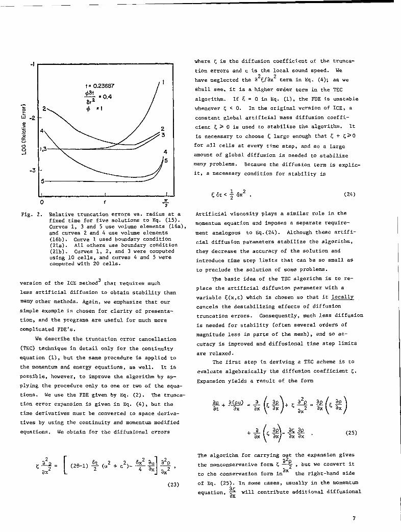
t= 0.23687+tlt— =0.4&2 /

I

2

t 23

,3 4

1 I I

u r _2

Fig. 2. Relative truncation errors vs. radius at afixed time for five soiutions to Eq. (15).Curves 1, 3 and 5 use volume elements (16a),and curves 2 and 4 use volume elements(16b). Curve 1 used boundary condition(21a). All others use boundary condition(21b). Curves 1, 2, and 3 were computedusing 10 cells, and curves 4 and 5 werecomputed with 20 cells.

3version of the ICE method that requires much

less artificial diffusion to obtain stability than

~nY other methods. Again, we emphasize that our

simple example is chosen for clarity of presenta-

tion, and the programa are useful for much more

complicated FDE’s.

We describe the truncation error cancellation

(TEc) technique in detail only for the continuity

equation (l), but the same procedure is applied to

the momentum and energy equationa, as well. It is

possible, however, to improve the algorithm by ap-

plying the procedure only to one or two of the equa-

tions. We use the FDE given by Eq. (2). The trunca-

tion error expansion is given in Eq. (4), but the

time derivatives must be converted to space deriva-

tives by using the continuity and momentum modified

equations. We obtain for the diffusional errors

where c is the diffusion coefficient of the trunca-

tion errors and c is the local sound speed. We

have neglected the 32</3x2 term in Eq. (4); aa we

shall see. it ia a higher order term in the TEC

algorithm. If ~ = O in Eq. (l), the FDE is unstable

whenever c < 0. In the original version of ICE, a

constant global artificial mass diffusion coeffi-

cient < > 0 is used to stabilize the algorithm. It

is necessary to choose E,large enough that ~ + L>O

for all cells at every time step, and so a large

amount of global diffusion is needed to stabilize

many problems. Because the diffusion term is explic-

it, a necessary condition for stability is

C6C<+6X2 . (24)

Artificial viscosity plays a similar role in the

momentum equation and imposes a separate require-

ment analogous tO Eq.(24). A-l-thoughthese artifi-

cial diffusion parameters stabilize the algorithm,

they decrease the accuracy of the solution and

introduce time step limits that can be so small as

to preclude the solution of some problems.

me basic idea of the TEC algorithm is to re-

place the artificial diffusion parameter with a

variable C(x,t) which is chosen so that it locally

cancels the destabilizing effects of diffusion

truncation errors. Consequently, much less diffusion

is needed for stability (often several orders of

magnitude less in parts of the mesh), and ao ac–

curacy is improved and diffusional time step limits

are relaxed.

The first step in deriving a TEC scheme is to

evaluate algebraically the diffusion coefficient C.

Expansion

>+at

yields a result of the form

(25)

(23)

The algorithm for carrying out the expansion gives

~ but we convert itthe nonconservative form C ax2 ‘to the conservation form in the right-hand side

of Eq. (25). In some cases, usually in the momemtum

~ will contribut‘quation’ ax e additional d~ffusional

7

errors that should be included in TEC as discussed

by Rivard et al. In our continuity equation,

~ doea not produce additional diffusional‘owever’ axerrors, and the

~~ax ax truncation error ia neglected.

In order to obtain an improved FDE, Eq. (23) is

difference to yield

[ci_%= (2e-1)$ (u;_%)2++(C2+C 1;_l)

Next we choose

(26)

which is then incorporated in the finite difference

form of Eq. (l). The constant f3,O < ~ < 1, is a

free parameter that determines the degree to which

the dlffusional truncation errors are cancelled. If

@ is too small, the l?DE’swill have so little diffu-

sion that dispersively generated ripples destroy

accuracy, If, on the other hand, B is too large,

unnecessary artifical diffusion reduces the accuracy

of the solution. The optimum value of 6 is problem

dependent and must be found by trial and error. In

practice, f3= 1 is frequently an adequate value.

Although the derivation of the diffusion errors

for the TEC schane requires extra work, the modified

FDE’s yield substantially better solutions, TEC has

been installed in several programs, and the scheme

worka well except in problems with very strong shocks

where higher order errors are significant. We now

briefly compare several TEC and non-TEC solutions in

order to show the advantage that may be expected

from using TEC.

Consider Fig. 3, which shows the run of density

for three one-dimensional shock tube calculations,

as well as the analytic solution.

tion is a 5:1

All solutions

8

pressure and density

coincide at the left

The initial condi-

jump at cell 90.

and right bound-

aries; the solutiona have been displaced vertically

for clarity. The bottom curve Is the analytic solu-

tion. ‘he top solution is an artificial viscosity

solution with nearly the minimum diffusion needed

for stability. The right density jump is a shock

wave, and the left discontinuity is a contact sur-

face. Both discontinuitiesmove to the right. The

shock is smooth, but the contact surface has disper-

sively driven ripples behind it. TEC.with the same

viscosity u as the conventional method,was used in the

second solution from the top. The shock is unchanged,

but the ripples behind the contact surface are atron-

ly damped. The third numerical solution is also TEC

run, but the viscosity is reduced by a factor of ten.

The shock is significant sharper, but it shows a

little overshoot. The first peak behind the contact

surface is as high as in the artificial viscosity run,

but the damping behind the contact is much stronger.

The artificial viscosity scheme is unstable with this

little viscosity.

The TEC algorithm readily generalizes to multi-

dimensional flows. As an example, consider a Mach

0.1 wind blowing over a pair of walls as shown in

Fig. 4. Shown there are the velocity vectors and

isotherms of a TEC solution obtained from the two-

dimensionalRICE program.’ The comparison solution

with normal artificial viscosity stabilization was

obtained with 100 times as much viscosity, because

“10

9 –

8 -

C=O.8*w= I.o

TEC I,L* 1.0%-ms TEc/.4=o.lE4 - Analytic

3 -

2 r

I

0 I I I I [ I I I I 1 I I I I I I I I

0 20 40 60 00 Im 120 140 160 180Cell Number

Fig. 3. One dimensional shock tube calculations.All four solutions coincide at the left andright ends, but the three numerical solu-tions have been displaced vertically forclarity.

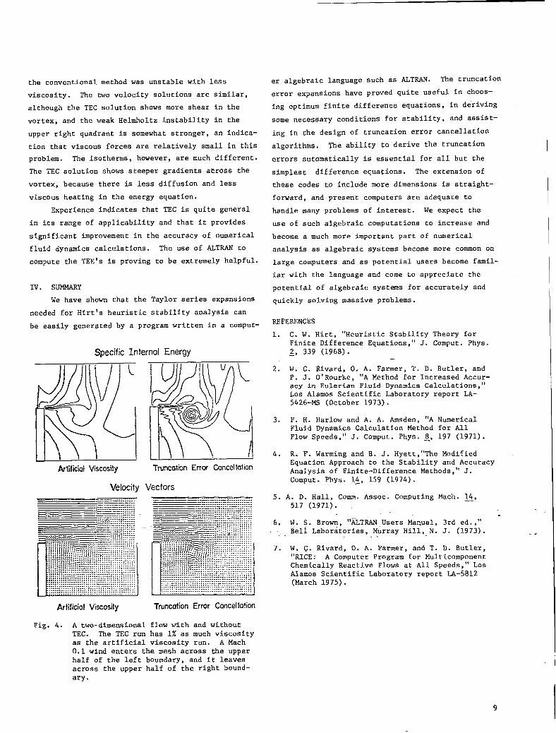
the conventional method was unstable with leas

viscosity. The two velocity solutions are similar,

although the TEC solution shows more shear in the

vortex, and the weak Helmholtz instability in the

upper right quadrant is somewhat stronger, an indica-

tion that viscous forces are relatively small in this

problem. The isotherms, however, are much different.

The TEC.solution shows steeper gradients across ‘the

vortex, because there is less diffusion and less

viscous heating in the energy equation.

Experience indicates that TEC is quite general

in its range of applicability and that it provides

significant improvement in the accuracy of numerical

fluid dynamics calculations. The use of ALTRAN to

compute the TEE’s is proving to be extremely helpful.

Iv. suMMARY

We have shown that the Taylor series expansions

needed for Hirt’s heuristic stability analysis can

be easily generated by a program written in a comput-

SpecificInternal Energy

[“

~[

&y\/J

\ArlificidViscosity Trunco\ionError Concellatian

Velocity

ArtificialViscosity TruncationErrorCancellation

Fig. 4. A two-dimensional flow with and withoutTEC. The TEC run has 1% as much viscosityaa the artificial viscosity run. A Mach0.1 wind enters the mesh across the upperhalf of the leftacross the upperary.

boundary, and it lea&half of the right bound-

er algebraic language such as ALTRAN. The truncation

error expansions have proved quite useful in choos-

ing optimum finite difference equations, in deriving

some necessary conditions for stability, and assist-

ing in the design of truncation error cancellation

algorithms. The ability to derive the truncation

errors automatically is essential for all but the

simplest difference equations. The extension of

these codes to include more dimensions is straight–

forward, and present computers are adequate to

handle many problems of interest. We expect the

use of such algebraic computations to increase and

become a much more important part of numerical

analysis as algebraic systems become more common on

large computers and as potential users become fsmil-

iar with the language and come to appreciate the

potential of algebraic systems for accurately and

quickly solving masaive problems.

REFERENCES

1.

2.

3.

4.

5.

6,

7.

C. W. Hirt, “Heuristic Stability Theory forFinite Difference Equations,” J. Comput. Phys.~, 339 (1968).

W. C. Rivard, O. A. Farmer, T. D. Butler, andP. J. O’Rourke, “A Method for Increased Accur-acy in Eulerian Fluid Dynamics Calculations,”Los Alamos Scientific Laboratory report LA-5426-MS (October 1973).

F. H. Harlow and A. A. Amsden, “A NumericalFluid Dynamics Calculation Method for AllFlow Speeds,” J. Comput. Phys. ~, 197 (1971).

R. F. Warming and B. J. Hyett,’’TheModifiedEquation Approach to the Stability and AccuracyAnalysis of Finite-Difference Methods,” J.Comput. Phys. ~, 159 (1974).

A. D. Hall, Comm. Assoc. Computing Mach. ~,517 (1971).

.- .W. S. Brown, “~TF&li Users Manual, 3rd cd.,”Beli Laboratories, Murray Hill, N. J. (1973). -..

W. ~. Rivard, O. A. Farmer, and T. D. Butler,“RICE: A Computer Program for MulticomponentChemically Reactive Flows at All Speeds,” LosAlamos Scientific Laboratory report LA-5812(March 1975).

I

I

9

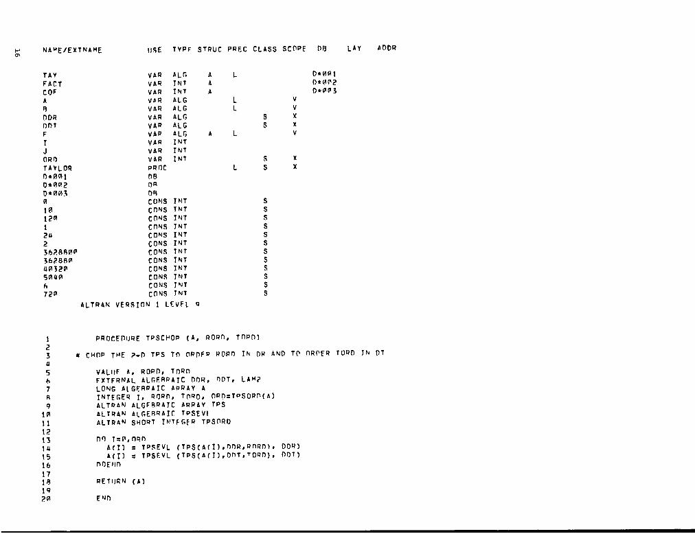
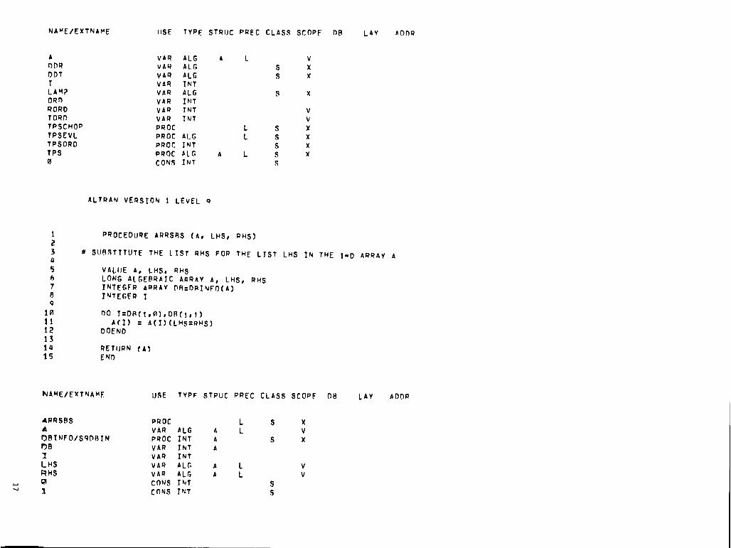
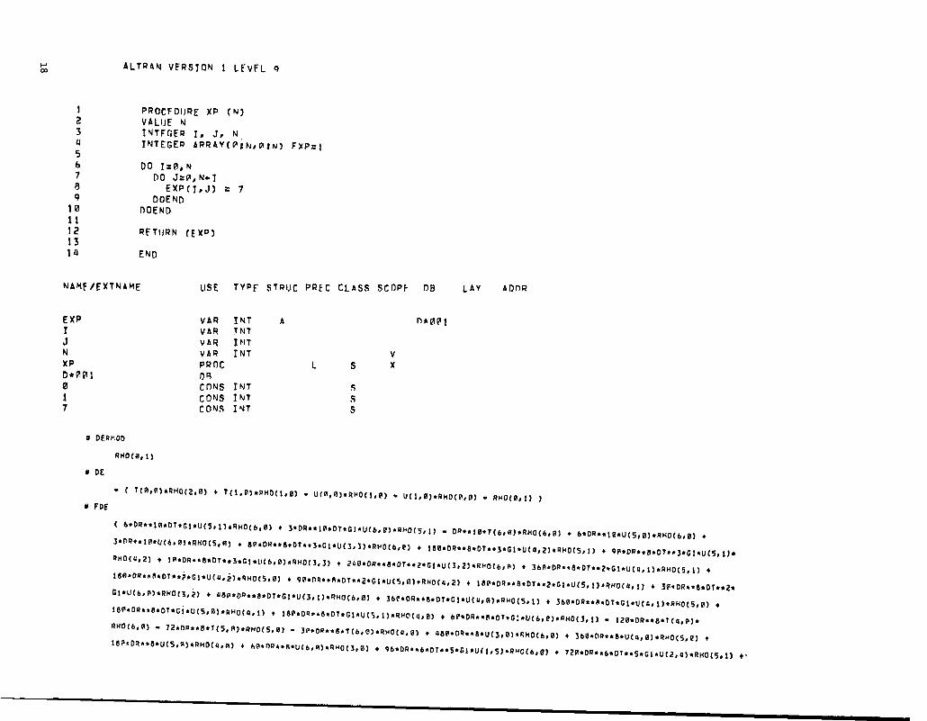
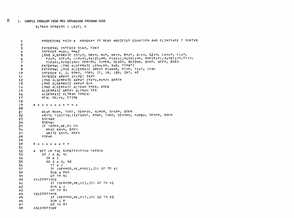
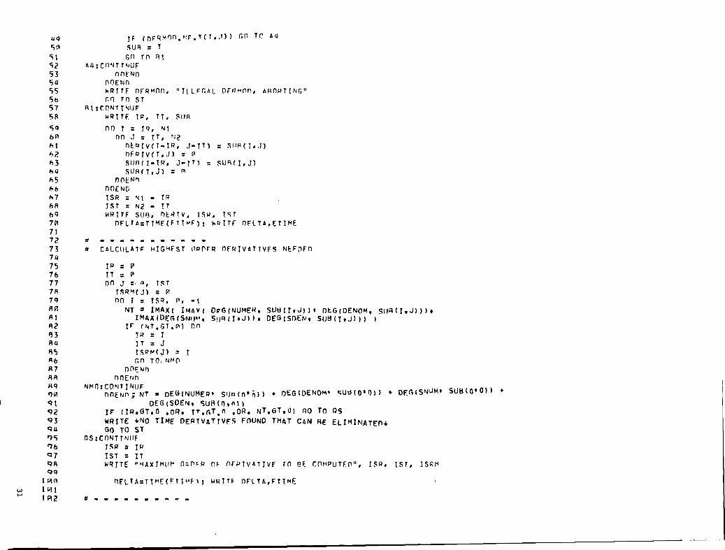
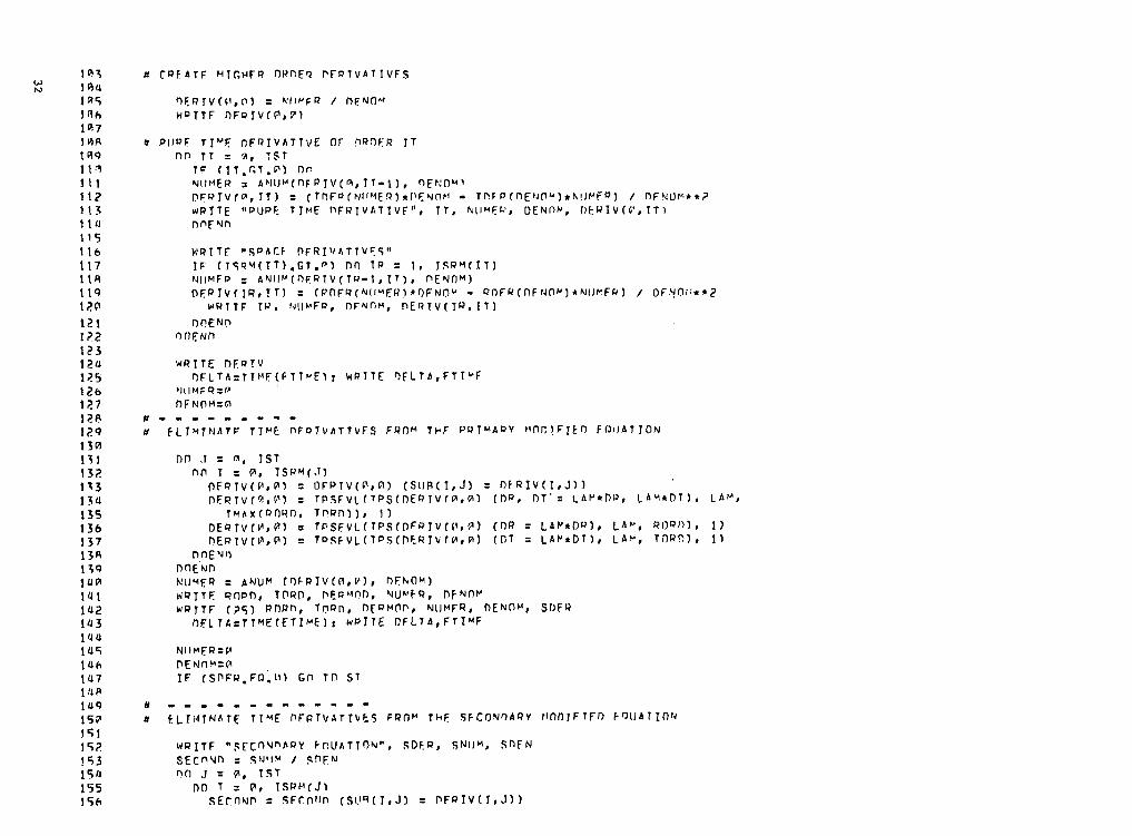
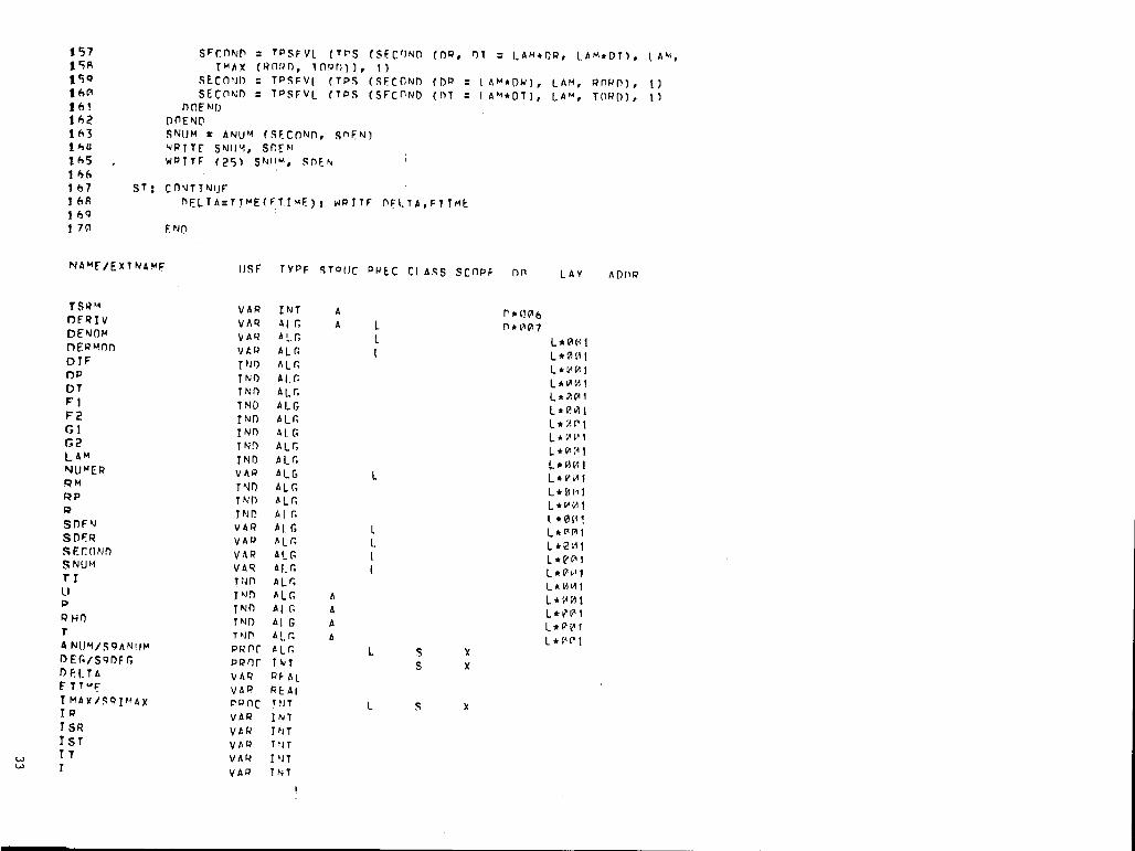
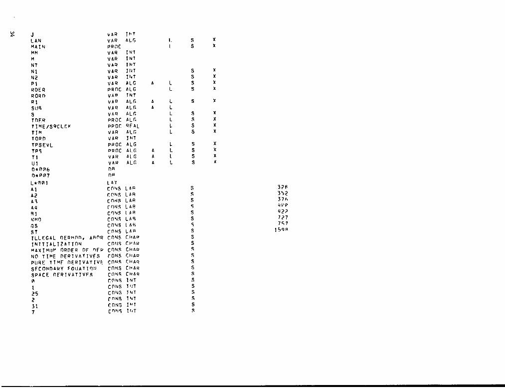
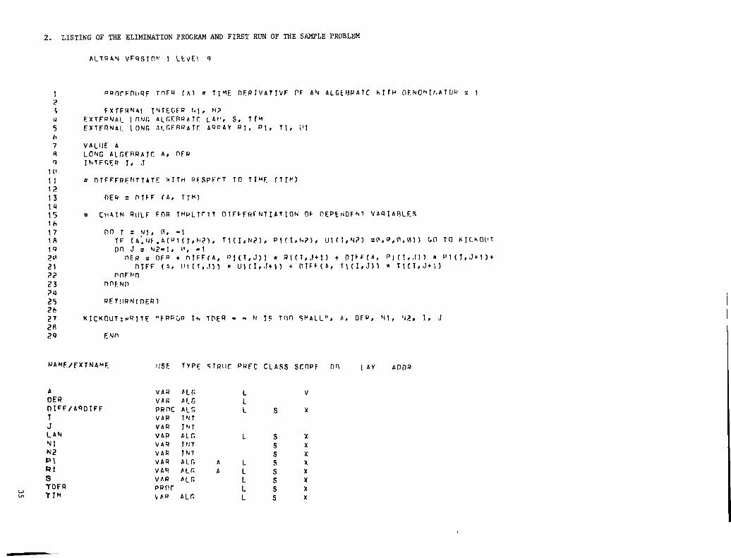
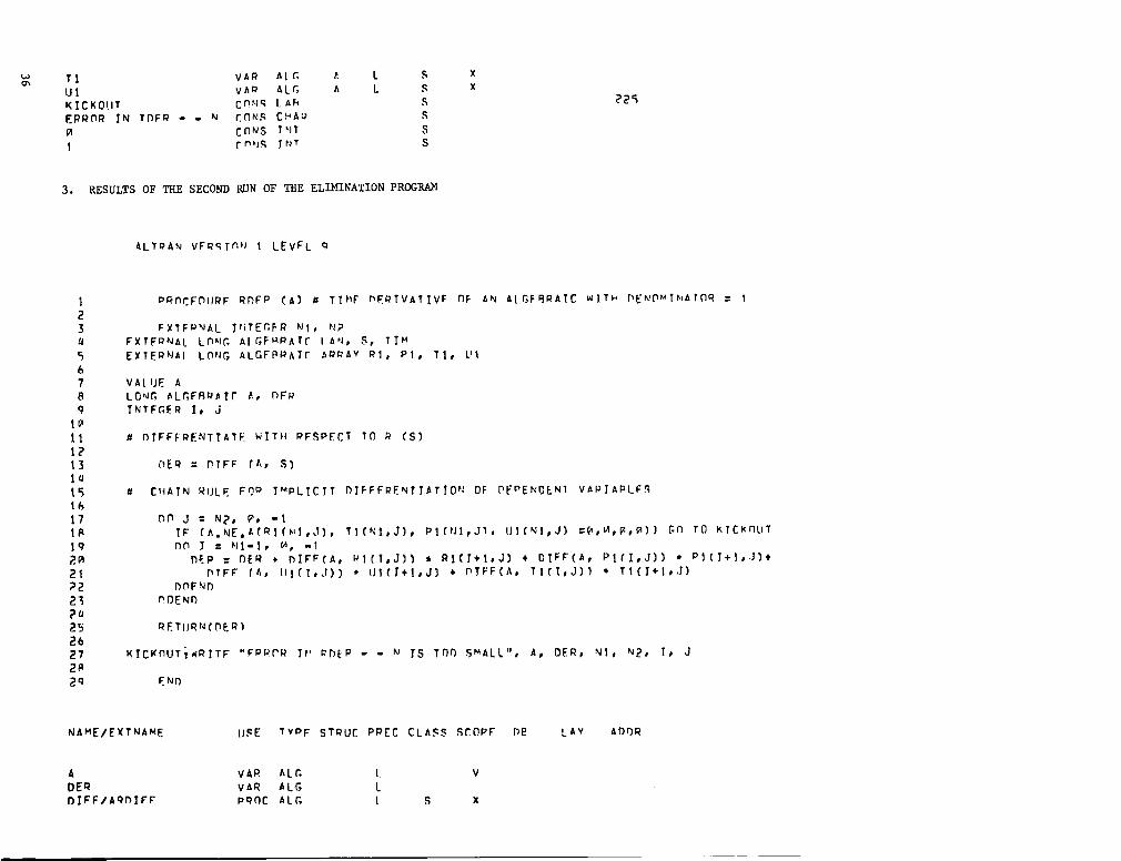
APPENDIX A

THE EXPANSION CODE LISTING

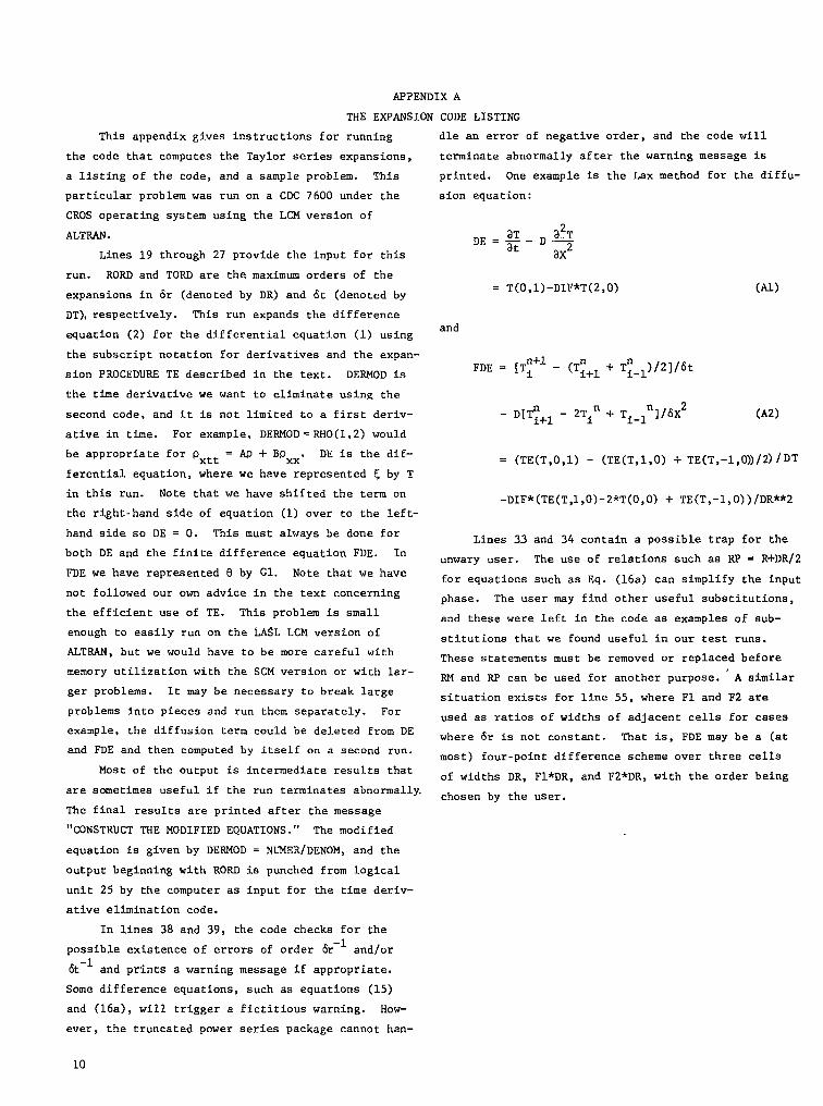
fiis appendix gives instructions for running

the code that computes the Taylor series expansions,

a listing of the code, and a sample problem. This

particular problem was run on a CDC 7600 under the

CROS opersting system using the LCM version of

ALTRAN.

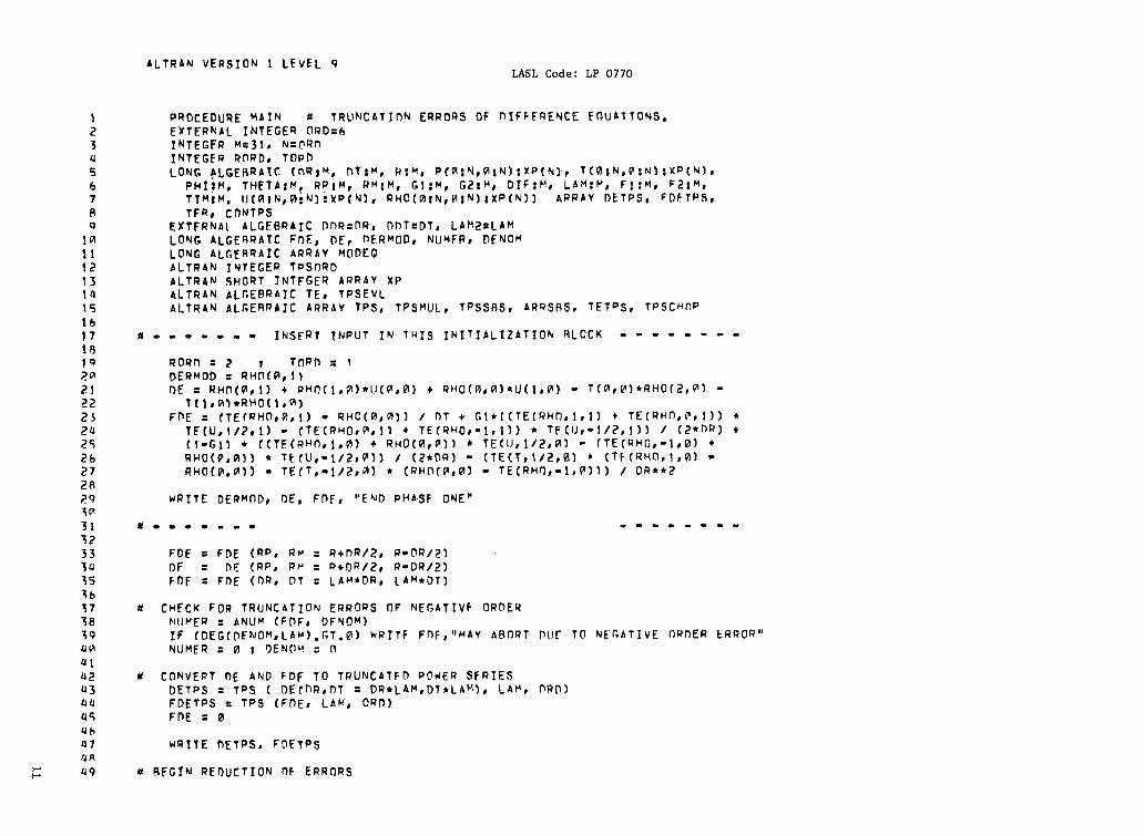
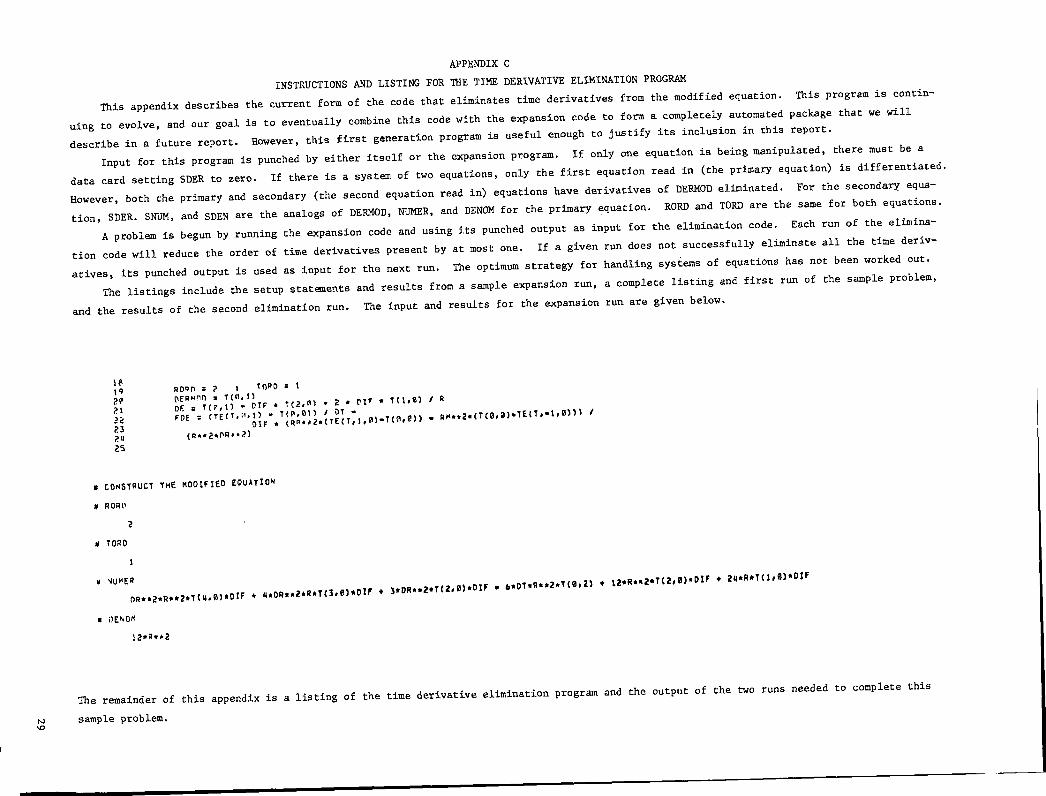
Lines 19 through 27 provide the input for this

run. RORD and TORD are the maximum orders of the

expansions in & (denoted by DR) and fit(denoted by

DT),respectively. This run expands the difference

equation (2) for the differential equation (1) using

the subscript notation for derivatives and the expan-

sion PROCEDURE TE described in the text. DERMOD iS

the time derivative we want to eliminate usin~ the

second code, and it Is not limited to a first deriv-

ative in time. For example, DERMOD=RHO(1,2) would

be appropriate for Pxtt = AP + BPXX. DE is the dif-

ferential equation, where we have represented ~ by T

in this run. Note that we have shifted the term on

the right-hand side of equation (1) over to the left-

hand side so DE = O. This must always be done for

both DE and the finite difference equation FDE. In

FDE we have represented 9 by G1. Note that we have

not followed our own advice in the text concerning

the efficient use of TE. This problem is small

enough to easily run on the LA$L LCM version of

ALTRAN, but we would have to be more careful with

memory utilization with the SCM version or with lar–

ger problems. It may be necessary to break large

problems into pieces and run them separately. For

example, the diffusion term could be deleted from DE

and FDE and then computed by itself on a second run.

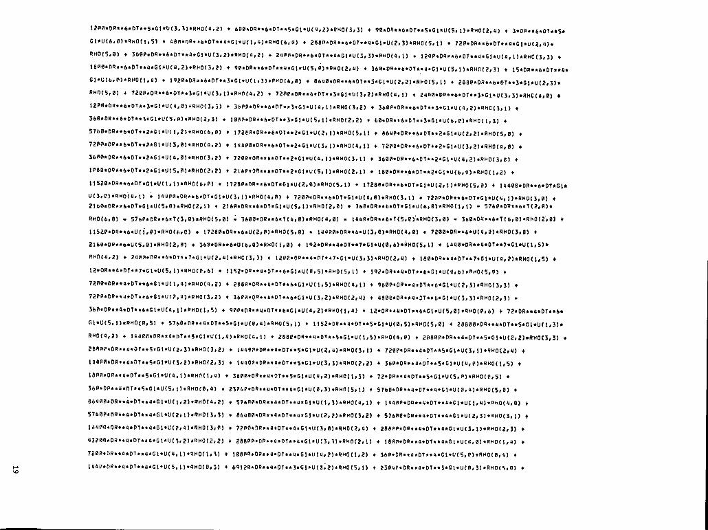
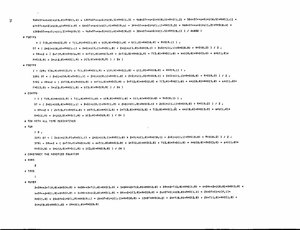
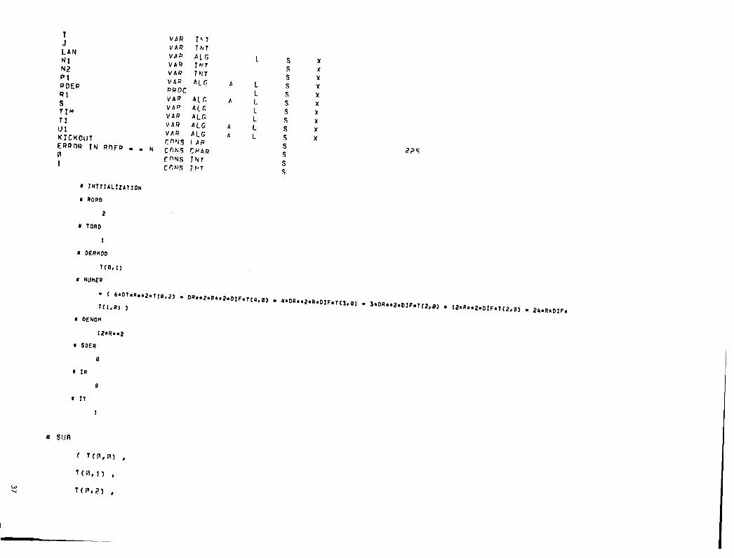
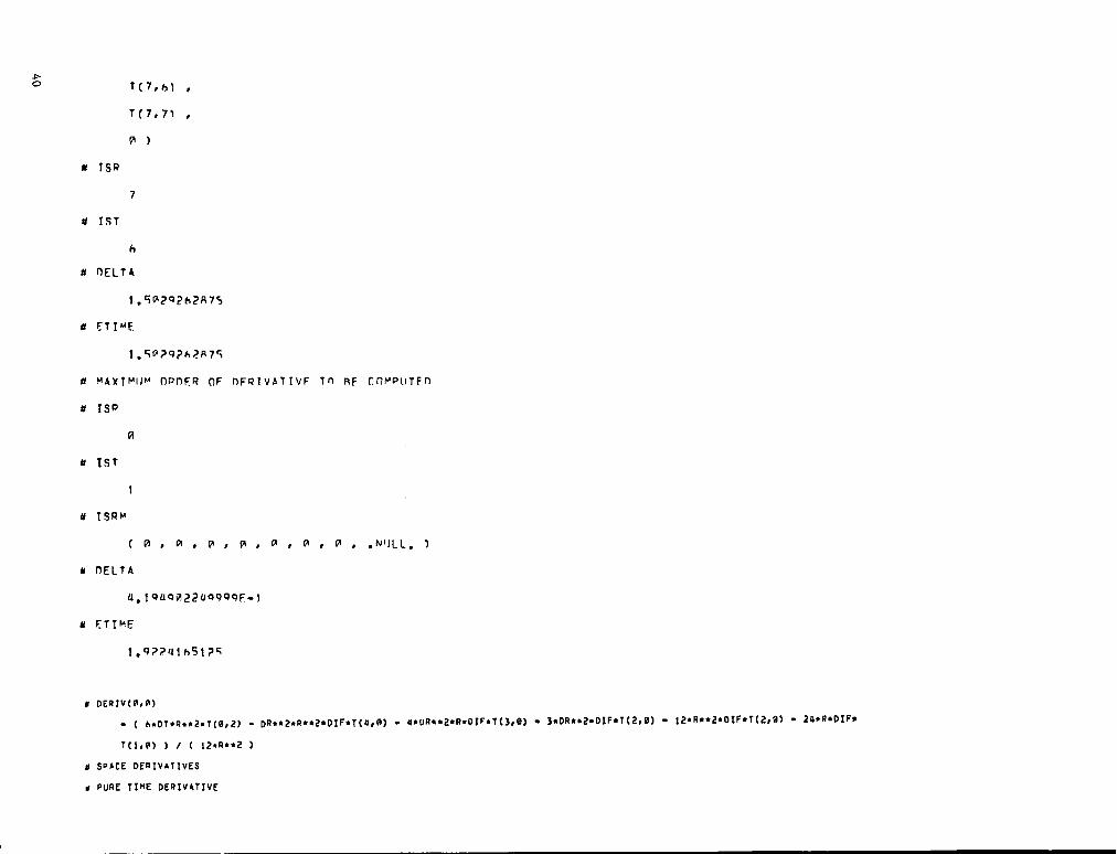
Most of the output is intermediate results that

are sometimes useful if the run terminates abnormally,

The final results are printed after the message

“CONSTRUCT THE MODIFIED EQUATIONS.” The modified

equation is given by DERMOD = NDMER/DENOM, and the

output beginning with RORD is punched from logical

unit 25 by the computer aa input for the time deriv-

ative elimination code.

In lines 38 and 39, the code checks for the-1possible existence of errors of order 6r andlor

&-l and prints a warning message if appropriate.

Some difference equations, such as equations (15)

and (16a), will trigger a fictitious warning. How-

ever, the truncated power series package cannot han-

10

dle an error of negative order, and the code will

terminate abnormally after the warning message is

printed. One example is the Lax method for the diffu-

sion equation:

DE=fl_D&at

ax2

= T(0,1)-DIF*T(2,0)

and

(Al.)

n+lFDE = [Ti - (T;+l+T;-1)/2]/6t

- DIT;+l - 2Tin + Ti_ln]/6X2 (A2)

= (TE(T,O,l) - (TE(T,l,O) +TE(T,-l,o))/2)/DT

-DIF*(TE(T,l,O)-2*T(0,0)+ TE(T,-l,o))/DR**2

Lines 33 and 34 contain a possible trap for the

unwary user. The use of relations such as RP = R+DR/2

for equations such as Eq. (16a) can simplify the input

phase. The user may find other useful substitutions,

and these were left in the code as examples of sub-

stitutions that we found useful in our test runs.

These statements must be removed or replaced before

RM and RP can be used for another purpose. ‘A similar

situation exists for line 55, where F1 and F2 are

used as ratios of widths of adjacent cells for cases

where 6r is not constant. That is, FDE may be a (at

most) four-point difference scheme over three cells

of widths DR, F1*DR, and F2*DR, with the order being

chosen by the user.

*+

..

--r.

Zrx

-.t-

nnl.uXkn

..

1A

(A$vw)

at-

-6.N0xa●s.s1-8s.

.(nz0

.-..

2=.

..

..

a

E-n-I&+

Zbu

--

-cSS..-.

>

.t-+n.

w+

\l----..

#-

-k*---15

-3.

..-m

a”

Cu.

-s.t

X+.

tu.

xN

-AC

-*>-X

U-

-W9--

.)-=--2”

UJ

u-.~+

*.iLlt-

cac.L&

xX

Oez

-lidIIG

Nz.

.cu-

0v)a0auw

..--x6X

-.“#..

Hcz-

Ztuzaa

-1*u..

nzz

..

.

.wza

zcc.

u.

nx>

u.

k4xx.

~*s..II

-

acw

CGu

-cfriu

zc

cl

c>.-

IL)(LW

*a.

+>

--Lx

U(X

o-u

18

WI

ucalxu4.cz0uo-U2uCY

zu0k.m

t-1-C

0t-U

J>G

aII

LAlz

Zc)

9-W

.4

k--X

Zw

luII

U.lz

adD-a

QZ

IL,uacs

UklluG

+t-axz

nuJ-

c....

Zs

Crxfilb

Laa

-I-uzD

-W

um

ua

D-o

-$&l&

-x-x

o+m

aw

wlrw

au+cic

Ww

zz-1

0C9

-(C-I

J4aazzz

zz’

I--V)

lu6a

x-I-I-=

2c

..Ux

x

A.

z09-I

-1

II

b-

.ax

8Itat

11

.n

c

a-IA

10>a

-

-)

xuzua

-JLLIr

.+.

l-

.-)-

-z

--X-*-lJ

..<-u-lN

nxh.++..Ll

--C

7Z

k.-.J

lz>W

.ut-

(nV

.=an

t-l-.

w-cc

Ca

iLcn!-

-R.z*C

Lou

ml

U-J

.U

m(o

Czo

.n

Xx

xxx

.x-1-1n

-xc

-lCr

.0

U)m

:.idcc

Cn

LLl--Id

.c=m

.W

,

:I&

cacxuOY

n.

)-11

W.

ao-

ldc

-lE>&u.

:>:aI-G-x

i-

trmnoouoac.

oc

cnoaaonaeon

~~

afr~aa-cru

a.azzz6zzzzzzzzzazzzz

zzaaaaa-ee-x

>>-

UU

>-I-U

-0-+

0-.-9

-9+>s+

--$8-D-fnafi

>>&

>>>

>

vU

3cn

nn

D-t-

Innt-6

?-t-iu

wIlc

cLAu.

(0ClllLu

b-l-

2b.

IIII

(nc

can

LL

ccIA.

IL

h.1t-

0zu

Z(X

Wcu

mV

b-x

v

ux-az

12

..“c.

*c.

xc.

c

.+0

.xc

1.u

.t-V.

x~

.u

b-

Z/2-.

x

%X

nxxmm

2-I

.)-m.

xm.

m

..

c-U

JrnvlL

..

l-xUti.

Xn-w

u-o

-a.

.uIzo-U

..LA

JM

x+

..m

-l+-l>>(r

.-xii.

.>tia

tnX

u-tx

a.

Irff..7)-

.rxx

m<auu

w.

.Uuua

l-b-+-a

m.a

--xm

a.&

lzww

Xc

ffimc

Uw

w-ld

.uL--I-t

-I-I-Ja

<zz

.?-5.

.k-

xm.

02--l

--a.*6

-1w>

.x-id)-“=”u(nE

t-1><t-GA

l

z0

u!

<a

3ciulYtx_lzz

)-t-40

CJ-I

>_J-t--

za

x

)-0.E.n

tY:*

.1-

0.

)-0.

xc.

C2.

I-v.

xu.

u

.t-U

’.xu.

02.

+4.

*X4.

uv,n.

$-Ld)-Wm!2U.1

G:a

xv.v

mn

-1

z?.WY

anc+

..0

!+C

u-l.>

x-l

u)-

>>

>>

>>

>>

>>

>>X

xx

>>

>>

>>

>>

>>

>

+e.

x6.

<

m

WIna-1u

L1-

V,

v.u

)v.

.+a.

xQ.-i

..

xc

-wU

.+a

.Ulc

+U

.-b.lm

%+

=c-1><)-2lx=1-.Lz.tr-12z

<u<

u<

.-m

F-Q

>(r

.<.>

t-tkx-z-cm

ma

.-x

-Q%

X-Q(J

..L

JV

Qt-u

-a6465

-a-a

uX

trffiwl

-1ldLd

-1.(30<

-1-i-l**2?Id=W

lu:d

zzk-U

cc

d>-l-la

*a

-l

u

VI

ao-

01N

LL.

14

-.K

n6

an

lO

*.

-(5-n

6-.

.w=

-m

k.-.CII

.->ru

6a

.&I--&

.----c

2---

trllu0

+1

8-(J

U.

ILu

uc-ii-u

>>

z6<--

>%

XXX

Cn

wto

Ln

Cr

cc:

Q

.t-.a

*7

-1-I

A-l

o-

nc

.

:?2cC

7U

C.

u.u-

U’

+.IA

u>2

>w3t

-a

Vu

uu

aocco

-zaafya

>nnna

>-z

+-

0n—>

cl)<

-trl-6.

C-

w

IIzo

11

0.It

v.aw>

.c?L

&l

.1

:u

nzEe

mL--

Go

cczaab-

IAu

15

-NW

SEESSci*U

*0C

C2

>>

XX

>XX

a-z-l

Q

0’

Cnw

tnlnlnmlc

co

wU

.o?u?

txam

czaafk

rxa

aa

=

-1

ZzzzzzzzZzzz

-Ia-t-a

-Iu-xaa

ae

fxma

rrac

cc

oo

oo

oo

oc

->>>>>>>>>>

>Qc

cnuuuuu

uuuouuo

z

c

Qu.cQGct-(#)n*cItid11-

ncxu

I-11

Gc.

(nc

an

c+

occ

cW

U.u

ce

ua=LA

.c

luatrfx

-J+’zo

-)-b-l-

UX

oz-1-l-l

>W-lu

u-la

..

fxo-

0C2

Oc.

.z)-C

cc

o..

--u..-aQ

.-rom

aa

+1-

.-

-1-1>>W

u!u.

Wa

mc

++

:II

1)“*zu=l-cW

zm

w

16

>u-1>aA

al

ca

)c

>Xxx

>>

XXXX

X>x

>>

-1wmxfx

vuan

-J-i-l

_l.mx-

J*

u=a1-ln

.mx-1-c

<IL

z>$

-

::C

nlx

uXam

txcv

-x

--l-t-x

(n-x-a.

II-

cc,

-x

ad

e-..-.*6

-.<

--M

an-18

H0

u-z

<u

00

(20

0“r,

.uk

Lo

z0.VI

au>

xmc

2u

17

02.+

asa>-xA

u.z

.L

t%IJIn

>X

(n(cV

.in

+cc

mQdu

-J

A!

xu.

..

u“z

Li>

,s..z

r-

-I

{M

mmIv

z.

Z&-z

.Ilac

S9X

ZII

iuwn

-10c

Zifi

00

nc

nx

,4

.u

,,:1

zIT

r1.4:ic

L>;

x

18

.+

*.

+

+

19

.

●

.3●

+

●

Gu’

--

20

+

.a...0.mz.N

+

+.+

.

21

.

+

+.02..8

D

8

*.5’I-

.

8.6

.a.m

w

22

.

+

0z.+*+

.

,-0::..2.

+

.

23

a

..a:

.

+

.+

+

a“+...+a-

.-+

.w,-az:

Inn.

.zc1v.

U:a.

24

zQnLIY***

v)u.t-ul

ua)-ln

-1uua6

ac

cJ

cil*

.O?--N

U.

N6

In.-

3=3

Wl

u-.

25

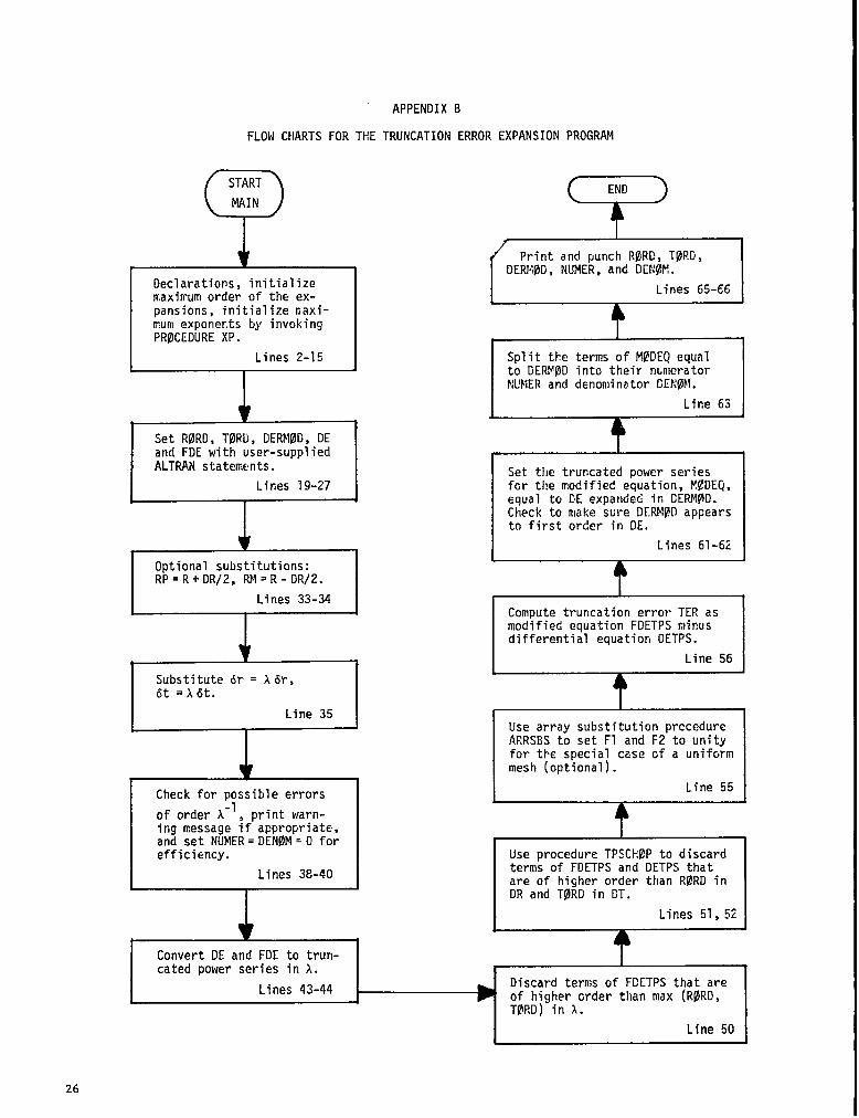
APPENDIX B

FLOW CHARTS FOR T1-!ETRUNCATION ERROR EXPANSION PROGRAM

7START

MAIN

w

Declarations, initializemaxitrumorder of the ex-pansions, initialize naxi-nwm exponer.ts by invokingPRfJCEDURE XP.

Lines 2-15

Set RORD, TORLJ,DERMOD, DEand FDE with user-suppliedALTRAN statements.

Lines 19-271

I Optional substitutions:RP=R+DR/2, RM=R-DR/2. I

YEND

‘ Print and punch RfJRC, TfWD,DERlfl$D,NUMER, and DEK!W.

Lines 65-66

t

Split the terms of MJ?DEQequalto GERVOD into their nm?ratorNIJMERand denominator CEN@M.

J Line 63I

Set.tiletruncated power seriesfcrtkemoc!ified equation, KCDEQ,equal to EE expanded itiCERM@D.Check to make sure DERNfKlappearsto first order in DE.

I Lines 61-62

Lines 33-34I

1

I Commte truncation error TER as

+ +

mod’ifiedequation FDETPS minusdifferential equation DETPS.

Check for possible errors-1

of order A , print warn-ing message if”appropriate,and set NUMER=DEN@M=O forefficiency.

Use array substitution prccedureARRSllSto set F1 and F2 to unityfor the special case of a uniformmesh (optional).

Line 55

Use procedure TPSCklZ?Pto discardterms of FDETPS and DETPS thatare of hicjherorder than R9RD inDR and TORO in DT.

Discard terms of FCETPS that areof higher order than max (RORD,T@RD) in 1.

I Line 50 I

26

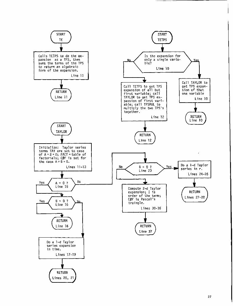
QSTART

TE QSTART

TETPS

Calls TETPS to do the ex-pansion as a TFS, thensums the terms of the TPSto return an algebraicform of the expansion.

Line 11

I

(5RETURNLine 11

START

TAYLOR

Initialize: Taylor seriesterms TAY we set to caseof A=B=O; FACT =table offactorials; COF is set forthe case A=B=O.

Lines 11-131

*

Is the expansion foronly a single varia-ble?

Line 10

Call TETFS to get TPSexpansion of all butfirst variable; callTAYLOR to get TPS ex-parisionof first vari-able; call TPSMUL tomultiply the two TPS’Stocjether.

Line 12I

ARETURN

w

vYes

I

Line 15

‘ies

f

ANo 6=0?

>

YesLine 23

+

Compute 2-d Taylorexpansion; I isorder of the term;COF is Pascal’straingle.

%1Lines 30-36

● 1

w 1x

Do a l-d Taylorseries expamionin time.

Lines 17-19

uRETURN

Line 37

t

Call TAYLOR toget TPS expan-sion of thatone variable

Line 10

I

(sRETURNLine 10

DO a l-clTaylorseries in r.

Lines 24-26

27

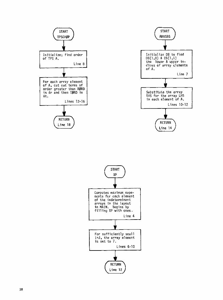
Ifiitialize;find orderof TPS A.

Line 8

For each array elementof A, cut out terns oforder greater than RORDin tirand then TORD in&t.

Lines 13-16

(5RETURNLine 18

START

ARRSBS

Initialize CB to findDll(l,O)& C6(1,1)the lower & upper in-c!ic~sof array elementsof A.

Line 74

I

Computes maximum expo-nents fcr each elementof the indeterminacyarrays in the layoutin MAIN. Begins byfilling XP with ones.

Substitute the arrayRHS for the array LHSin each element of A.

Lines 10-12

QSTART

XP

m

bRETURN

Line 14

(sRETURNLine 12

28

gP’!

c1zH5Hdz

Hjal

%01

20:u

.!5L!

rno

M.5u.:.-l

a

11

..#.8-$-:●:5.

awu.00x

.

tu

w0i3n0ua29

c

aN

mc

<<

t-C

c

.zc

ucsC

L.L>w-1

..

.

zcwLYc

=h.w

a5-

CG

l-tilnllv..

-x~ct=

6~z-tL

tYz

-I*=UI

axu

.LICYZC

ILc

LL>za+..

..mM

Qe

au

0.0

.<..u=v,

.LY

v..c*0

.

.cb,

cL4.

.&J

zv,u,>.+.>.xLc(YL

IL

n05

[*

1:858X

9M.

a:-J

Iz

8>

D:

a-a

Ozc-z

v

c

..

1-Z

L1-

<>

.-!r

-b

.

c’

..

c-m

-.0

ac.=-C

nC

c

*!t-IA

.c

It

8-.

.cL

-.*ZC

a:cZz

-ul--6

-~.

xlul-

$C

lm-.

)“●

t..2:.

:

9-1

a=,

u.

861-.

.

.E

.1-

t-+-3

II

n

xo

-t-.

.

u.cII

c.

2U.$

cCzCld

cc

.t-utJtLb

-2CZLL

J-:1

-15II

1-

w+‘aIMc

It

a

..u

c..

xw

zc

31

—

z0

m

*.zczw0

u.

.zczucX

l&-

c.x

zrcl-

hLLt-C

zb.=.

-.Z-s

-..>.

+.a1

aIA.

>cII

.--.-.

c-*

..

-ci

&L,

8-X

u?

L>1-Q>0-

L>Lc-

-)..

II-

.-u-a.

Ll,*-co

l..>

..

-c%C.Z

U!.t

-u,

c-

----

=.

--!-l>>->>-U

.c

luu.a

ma

mw

.-Laclia

-.o~

l-!-t-

:c.1?

wcEcl

l..xcx

..II+LI

cu.

.->

cc-.-llb

-<1--

I

)-ua.?.*C

-*ra-

cl-

-Ga

b$-c-

Zillu

3-Zc-:

<::;

Xltll

.1111a

cln.

-!r--

+-as

c6c

.

Itt-U.

h..-

*..->

L,*=<-z

2>

..7:(C

IIC

Z9-.

GW

6CLJ.

zC

r.l1511c

>cf,

G=-u,

0-!,-

.Z+n

e+a+x

I&.L’

.&C

6.115=

t-.-

.u

)-.

u.

m

ii

32

uvu

U..

-ULA

W,-

CC

WI

..

mL+II

.U

-W

.a

n!-l-.

.

zu.,cc

czin

GzLL

LU-J

=Id

xuz

.nt.

xxx

-1

-f_l._

<<

<U-.2

33

xxX

xxxx

Xxxx

v,(n

InC

ow

.rn

In*u.

lnvl

Xxxx

V31n

ultn

fx(i.L,CL.

ccu.

!!$C

zcc%

Zwu

at-c

Wua

CN

C.

u,u,>.

34

.

&ccu.,=.a.L&

au2.c

?Juzu2u.>

cc

>X

XX

xxxxxx

U.I

0W.-k

.z8

u.-

..-

*.c

--.w

f,-#-+

-

ZIA,

a>.

.xD-.

+..

uGk.

!5clx

3...--am

E4:

L.-

.rur=..

A-ZLI.

-z11k

2-.1)-<-c

c11--,

uz

cu.=

*LA-C

Cz

8-Cc

IL

cc

cc

.--wo-

rz%..

LA.

>74m

i-

va

Yvwx

I&zt-

0x

m

4

35

—

II

wc

v-(-U

&

z.

>*

xx

v..

u.

<iU.

V.

ICU

.WV

Y

+..C

u(n

-1

u.>

1!I.Q

05

uluJ

mb.cc?

ma:

U4C

J

>>a

ccv.

lov-

Ccnzzzz

<<c

Ccc

>>u

L’tJL.

wu;=

zb

.>zun)-Je

ccm

-—Ga

xc

Uz

4.wa

+zxws

-

36

zQ:Q!

zN

m-

.w

E.

.

37

Onthispageandthenext,thereadershouldbeawarethatthecolumns,

beginningwithT(0,3),

aretobereadasonecontinuousrun.

..-..

..

..

..

-....

..

●✍

✎✎

✎✍

..

..

..

..

-...

●✎

✎✍

✍✍

✍✍

✎✎

✎✎

✍

al

..

..

..

..

...=

..

..

..

..

.----

..

..

..

..

..

----.

..

..

..

..

..

..

..

..

..

...-.

..

..

..

.---

..

..

.

..

..

..s.

..

..

..

..

..

..

..

.

..

..-..

..

..

..

..

.n..

..

..

-.-..

.---

n-.----

r-

t-u?-

=lv

.&r-

.--n---

nvla

u-.

cT

-5

.n

’ra*lrla

r-.

..-..

..

..

..

..

.W

.4-O

.C<

*.G.c

l.r-r.

-*

br-

r--

U..

..

..

L-

E5

US

C2c

s.----

.Uu

..

..

-------

--

39

z.2!

.Lc

.6

.

6

.

6

cb.>h.c

N●

.6.

6

wn

t’un!

Saaw

In.c

:.r-t

u.

..

-.4?r-

..

?-b-.

.+)-s

aIdn.

I6

zQ

t-a

cl)

v.

mw

.

u..a(nx

40

w“

2awca

*kn.a●z8

D

.

..

..

..

..

---.

41

-...

..

.m

...-.

..

..

IbJ

c

r-

..

..

..

..

..

..

..

..

.---

...-

42

mCr

*,L-,

u.

z.

W

z<xcz

W.

-1zz.

t..

rr-mrvlx.

4-.

1-

_,2’a

-L-

t-VIc?.

c.(s1-

***

43

#;=.N.

,.:

?*.*.=

*

..●

,2

nn

%

●k0a

.

44

Onthispageandthenext,thereadershouldbe

awarethatthecolumns,beginningwithT(1,4),

aretobe

readasonecontinuousrun.

..-

-...---

.-*.---

..

..

*--

...*

-..

..----

..*..

..

●☛

✎✎

✎

------

------

----

----

lvl-l*In4)r

.(u

----.

.r)

*u,

@f-

“(u

r)e

u)

w1-

..*

ml

m.?

If).

.----

..

.-....*

00

g0“

00

.d

d-

.-Z

.+.-I

.t-u

ntN

t-kn

NN

.A

f-,~

m~.

..

..

---

---

---

---

----

---

-i-)-+

1-t-l-c)-

+>

+*I-J-

C*E

+L

-+

++

,---

--

i--k●

+

..

..*-*..

..

..

..***.-.

----_

a=u)w

**..*---

.**-----

-..*--m-

-*.

45

..

----.*-

..-..

..

00

..

Irm

nn

‘mn

-----

----*--

-.-***-

-----

..

..----

-------

-...

..

.-.

n

46

.0. ●=2

●D

1“.

..::nx’

*::N:1-

..c.c.c.c.0

.

c.nJ

.=.r,

I

●

3.u&

1n

an*

n

47

*\

!0.-.

●D

●

.-.

.*W.

m1-

.*rG-

+-C

.N.m1-

.u.CL

●W

.IN

..-m..+

..

.-.-.

.In.-00--*k

-.-‘n.08-

.,-r-.08-

1-

48

b.aG

uv

uPn**

“aC

fJ.,

-L

k)-UJ

1-

W

ns

un

*

..&.*1

-

.1-:1-

.*:1-

.U1.at-

...

.r-

C1

-

..m.f-t-

..0.1-&

1-

n

..-.*-.

...-

..-----

..

.*..

-------

---.-.

------

---*ru

rI*lnat-

ficuw*m

.o1

----

.tw

mu

mw

Jr-

-...-.

Nt-)

..

..

-.0.

..

..

..

mm

r;

mF’

v.-

e*

+*

4u

4-

ul

mm

ar

u’

r!-

e4

e.-.

---

---

----

---

----

---

-bet-l-fit-

t-c

b-kl-l-

**#-

c*t-

b-1-kkkr

)-*F

---

49

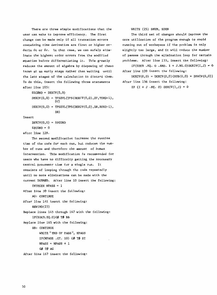
There are three simple modifications that the

user can make to improve efficiency. The firat

change can be made only if all truncation errors

containing time derivative are first or higher or–

derin dt or 6r. In that case, we can safely elim–

inate the highest order errors from the modified

equation before differentiating it. This greatly

reduces the amount of algebra by disposing of these

terms at an early stage rather than waiting until

the late stages of the calculation to discard them.

To do this, insert the following three statements

after line 105:

SECOND= DERIV(O,O)

DERIV(O,O)

i)ERIV(O,O)

Insert

DERIV(O,O)

SECOND = O

after line 129.

The second

= TPSEVL(TPS(DERIV(O,O),DT,TORD-l),DT)

= TPSEVL(TPS(DERIV(O,O),DR,RORD-1),

DR)

= SECOND

modification increase the runnine

time of the code for each run, but reduces the num-

ber of runs and therefore the amount of human

intervention. This modification is recommended for

users who have no difficulty getting the necessary

central processor time for a single run. It

consists of looping through the code repeatedly

until no more eliminations can be made with the

current DERM@D. After line 10 insert the following:

INTEGER NPASS = 1

After line 30 insert the following:

AG: CONTINUE

After line 141 insert the following:

REWIND(25)

Replace lines 145 through 147 with the following:

lF(SDER.EQ.O)G@ To BB

Replace line 165 with the following:

BB: CONTINUE

WRITE ’’ENDOF PASS”, NPASS

IF(NPASS .GT. 10) Go To ST

NPASS = NPASS + 1

GO To AG

After line 167 insert the following:

WRITE (25) SNUM, SDEN

The third aet of changes should improve the

core utilization of the program enough to avoid

running out of workspace if the problem is only

slightly too large, and it will reduce the number

of passes through the elimination loop for certain

problems. After line 133, insert the following:

IF(SDER .EQ. O .AND. I + J.NE.O)DERIV(I,J) = O

After line 139 insert the following:

DERIV(O,O) = DERIV(O,O)(SUB(O,O) = DERIV(O,O))

After line 156 insert the following:

IF (1 + J .NE. O) DERIV(I,J) = O

50

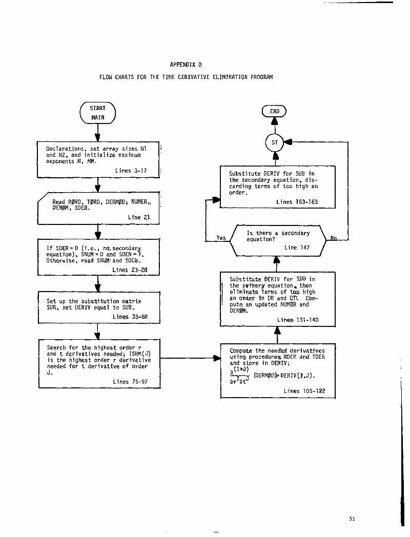
APPENDIX D

FLOW CHARTS FGR TFE TIME DERIVATIVEELIMINATIONPROGRAM

TSTART

MAIN

Declarat-iorls,set array sizes N1 ~and N2, and initialize rraximumexprments hl,MM.

I

(Read R@RD, TORD, DERM@D~ NUMER,,DENflM,SDER.

Line 23,

IIf SDER=D (i.e., n~se~ondanyequation), SNUM=O and SDEN=l’.Otherwise, read SNkiM’andSOEN.

Lines 23-28

kuuIEidSet up the substitution matrix

r

TEND

&-Substitute DEI?IVfcr SUB inthe secondary equation, dis-carding terms of triohigh anorder.

Lines 153-163I

IJ.J equation? bQ--1s there a secondary

Substitute DERIVfor UB inthe prrilr!aryequation~ thenelimirrak terms of t.mahighan o@w fn DR and DT(. Com-putew updated NUMER andDENflM:.

Lines 131-140

Search for the highest order rand t derivatives needed; ISRM(J) Compute the needed derivatives

is the highest order r derivative + ‘ using procedures RDEf?and TDER

needed for t derivative of order and store in OERIV;

J. ~(wl)

Lines 75-97 1~ (DERMODkDERIV(E,J).ar at

L I

I Lines 105-122

51

—

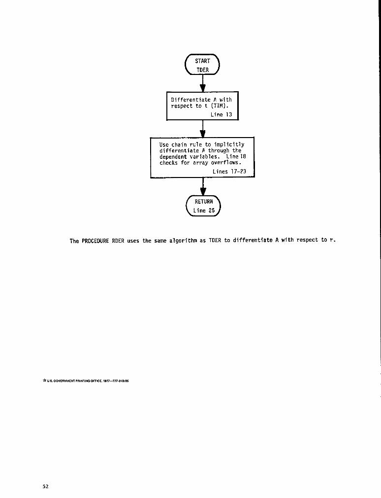
9START

TDER

Use chain rule to implicitlydifferentiate P through thedependent variables. Line18checks for array overflows.

Lines 17-23

I

(5RETURNLine 25

The PROCEDURE RDER uses the same algorithm as TDER to differentiate A with respect to r.

* U.8.CIOVEUNMENTPRINTIW OFFICE 1977-777.016/9’3

52