Embed Size (px)
Citation preview

AUTOMATED RADIO NETWORK DESIGN USING ANT COLONY
OPTIMIZATION
by
Jeffrey Allen Sharkey
A thesis submitted in partial fulfillmentof the requirements for the degree
of
Master of Science
in
Computer Science
MONTANA STATE UNIVERSITYBozeman, Montana
April 2008

c©COPYRIGHT
by
Jeffrey Allen Sharkey
2008
All Rights Reserved

ii
APPROVAL
of a thesis submitted by
Jeffrey Allen Sharkey
This thesis has been read by each member of the thesis committee and has beenfound to be satisfactory regarding content, English usage, format, citations, biblio-graphic style, and consistency, and is ready for submission to the Division of GraduateEducation.
Dr. John T. Paxton
Approved for the Department of Computer Science
Dr. John T. Paxton
Approved for the Division of Graduate Education
Dr. Carl A. Fox

iii
STATEMENT OF PERMISSION TO USE
In presenting this thesis in partial fulfillment of the requirements for a master’s
degree at Montana State University, I agree that the Library shall make it available
to borrowers under rules of the Library.
If I have indicated my intention to copyright this thesis by including a copyright
notice page, copying is allowable only for scholarly purposes, consistent with “fair
use” as prescribed in the U. S. Copyright Law. Requests for permission for extended
quotation from or reproduction of this thesis in whole or in parts may be granted
only by the copyright holder.
Jeffrey Sharkey
April, 2008

iv
ACKNOWLEDGEMENTS
I would like to thank Doug Galarus for providing me with an excellent problem
to solve, and for his guidance in the development of my solution approach. His focus
on making our theoretical results applicable in real-world scenarios has provided a
strong foundation for our research. I truly appreciate his time and guidance.
I am very grateful to the Western Transportation Institute (WTI) for extending a
graduate fellowship to me. Their financial support over the last two years has allowed
me to fully dedicate myself to this research. I would like to thank several people at
WTI for their help and technical insight, including Bill Jameson, Gary Schoep, and
Justin Krohn. Bill Jameson is an experienced radio engineer, and he was a great help
as I learned about radio systems and propagation algorithms.
I would like to thank Dr. John Paxton for his guidance as I prepared this thesis.
I am also thankful to Dr. Paxton, Dr. Neil Tang, Dr. Rocky Ross, and Doug Galarus
for all serving on my committee. I would like to thank Scott Dowdle for his help in
providing a powerful computing platform that I used to test my solution approach.
Without Scott’s help, I would still be waiting for my results to finish.
Finally, I thank and praise my Lord and savior Jesus Christ, with whom all things
are possible.
v
TABLE OF CONTENTS
LIST OF TABLES . . . . . . . . . . . . . . . . . . . . . . . . . . . . . . . . . . . . . . . . . . . . . . . . . . . . . . . . . . . . . . . . . . vi
LIST OF FIGURES . . . . . . . . . . . . . . . . . . . . . . . . . . . . . . . . . . . . . . . . . . . . . . . . . . . . . . . . . . . . . . . . . vii
ABSTRACT .. . . . . . . . . . . . . . . . . . . . . . . . . . . . . . . . . . . . . . . . . . . . . . . . . . . . . . . . . . . . . . . . . . . . . . . . vii
1. INTRODUCTION .. . . . . . . . . . . . . . . . . . . . . . . . . . . . . . . . . . . . . . . . . . . . . . . . . . . . . . . . . . . . . 1
2. PREVIOUS WORK.. . . . . . . . . . . . . . . . . . . . . . . . . . . . . . . . . . . . . . . . . . . . . . . . . . . . . . . . . . . . 4
Approximations . . . . . . . . . . . . . . . . . . . . . . . . . . . . . . . . . . . . . . . . . . . . . . . . . . . . . . . . . . . . . . . . . 4Steiner Graph Representation. . . . . . . . . . . . . . . . . . . . . . . . . . . . . . . . . . . . . . . . . . . . . . 6
Metaheuristics . . . . . . . . . . . . . . . . . . . . . . . . . . . . . . . . . . . . . . . . . . . . . . . . . . . . . . . . . . . . . . . . . . . 9Genetic Algorithms . . . . . . . . . . . . . . . . . . . . . . . . . . . . . . . . . . . . . . . . . . . . . . . . . . . . . . . . . 9Simulated Annealing . . . . . . . . . . . . . . . . . . . . . . . . . . . . . . . . . . . . . . . . . . . . . . . . . . . . . . . . 12Tabu Search . . . . . . . . . . . . . . . . . . . . . . . . . . . . . . . . . . . . . . . . . . . . . . . . . . . . . . . . . . . . . . . . . 12Ant Colony Optimization . . . . . . . . . . . . . . . . . . . . . . . . . . . . . . . . . . . . . . . . . . . . . . . . . . 13
Limitations . . . . . . . . . . . . . . . . . . . . . . . . . . . . . . . . . . . . . . . . . . . . . . . . . . . . . . . . . . . . . . . . . . . . . . 15
3. METHODOLOGY .. . . . . . . . . . . . . . . . . . . . . . . . . . . . . . . . . . . . . . . . . . . . . . . . . . . . . . . . . . . . . 17
Propagation Model . . . . . . . . . . . . . . . . . . . . . . . . . . . . . . . . . . . . . . . . . . . . . . . . . . . . . . . . . . . . . . 17Generalized Steiner Tree-Star Adaptation . . . . . . . . . . . . . . . . . . . . . . . . . . . . . . . . . . . . . 18Metaheuristic Formulation. . . . . . . . . . . . . . . . . . . . . . . . . . . . . . . . . . . . . . . . . . . . . . . . . . . . . . 23
4. RESULTS . . . . . . . . . . . . . . . . . . . . . . . . . . . . . . . . . . . . . . . . . . . . . . . . . . . . . . . . . . . . . . . . . . . . . . . . 29
Variables . . . . . . . . . . . . . . . . . . . . . . . . . . . . . . . . . . . . . . . . . . . . . . . . . . . . . . . . . . . . . . . . . . . . . . . . . 29Testing Scenarios . . . . . . . . . . . . . . . . . . . . . . . . . . . . . . . . . . . . . . . . . . . . . . . . . . . . . . . . . . . . . . . . 31
Relay Along Roadway . . . . . . . . . . . . . . . . . . . . . . . . . . . . . . . . . . . . . . . . . . . . . . . . . . . . . . 35Covering Roadway . . . . . . . . . . . . . . . . . . . . . . . . . . . . . . . . . . . . . . . . . . . . . . . . . . . . . . . . . . 37Adding Bandwidth and Delay Constraints . . . . . . . . . . . . . . . . . . . . . . . . . . . . . . . . 39
β Analysis . . . . . . . . . . . . . . . . . . . . . . . . . . . . . . . . . . . . . . . . . . . . . . . . . . . . . . . . . . . . . . . . . . . . . . . 42
5. CONCLUSIONS. . . . . . . . . . . . . . . . . . . . . . . . . . . . . . . . . . . . . . . . . . . . . . . . . . . . . . . . . . . . . . . . . 47
Future Work . . . . . . . . . . . . . . . . . . . . . . . . . . . . . . . . . . . . . . . . . . . . . . . . . . . . . . . . . . . . . . . . . . . . . 48
REFERENCES CITED .. . . . . . . . . . . . . . . . . . . . . . . . . . . . . . . . . . . . . . . . . . . . . . . . . . . . . . . . . . . . 50

vi
LIST OF TABLES
Table Page
1. Radio Sensitivity and Bandwidth . . . . . . . . . . . . . . . . . . . . . . . . . . . . . . . . . . . . . . . . . . 30
2. Assigned GSTS Node Variables . . . . . . . . . . . . . . . . . . . . . . . . . . . . . . . . . . . . . . . . . . . . 31
3. Assigned GSTS Edge Variables . . . . . . . . . . . . . . . . . . . . . . . . . . . . . . . . . . . . . . . . . . . . 31
4. Relay Along Roadway Scenarios . . . . . . . . . . . . . . . . . . . . . . . . . . . . . . . . . . . . . . . . . . . 36
5. Covering Roadway Scenarios . . . . . . . . . . . . . . . . . . . . . . . . . . . . . . . . . . . . . . . . . . . . . . . 38
6. Covering Roadway Scenarios with Constraints . . . . . . . . . . . . . . . . . . . . . . . . . . . 40

vii
LIST OF FIGURES
Figure Page
1. Example Wide-Area Network . . . . . . . . . . . . . . . . . . . . . . . . . . . . . . . . . . . . . . . . . . . . . . 2
2. Example GSTS Graph and One MST Solution . . . . . . . . . . . . . . . . . . . . . . . . . . . 7
3. Pheromones on Ant Trails. . . . . . . . . . . . . . . . . . . . . . . . . . . . . . . . . . . . . . . . . . . . . . . . . . 14
4. Example GSTS Construction Graph and MST Solution . . . . . . . . . . . . . . . . . 21
5. Example of ACO In Progress on a GSTS Graph . . . . . . . . . . . . . . . . . . . . . . . . . 26
6. Partial ACO Solution for US-199 Scenario . . . . . . . . . . . . . . . . . . . . . . . . . . . . . . . . 33
7. Partial ACO Solution for US-191 Scenario . . . . . . . . . . . . . . . . . . . . . . . . . . . . . . . . 34
8. Unconstrained MST Solution . . . . . . . . . . . . . . . . . . . . . . . . . . . . . . . . . . . . . . . . . . . . . . 41
9. Constrained MST Solution . . . . . . . . . . . . . . . . . . . . . . . . . . . . . . . . . . . . . . . . . . . . . . . . . 41
10. β Analysis for US-199 (a) Scenario . . . . . . . . . . . . . . . . . . . . . . . . . . . . . . . . . . . . . . . . 43
11. β Analysis for US-199 (b) Scenario . . . . . . . . . . . . . . . . . . . . . . . . . . . . . . . . . . . . . . . . 44
12. β Analysis for US-191 Scenario . . . . . . . . . . . . . . . . . . . . . . . . . . . . . . . . . . . . . . . . . . . . 44
13. β Analysis for US-101 Scenario . . . . . . . . . . . . . . . . . . . . . . . . . . . . . . . . . . . . . . . . . . . . 45

viii
ABSTRACT
Radio networks can provide reliable communication for rural intelligent trans-portation systems (ITS). Engineers manually design these radio networks by selectingtower locations and equipment while meeting a series of constraints such as cover-age, bandwidth, maximum delay, and redundancy, all while minimizing network cost.As network size and constraints grow, the design process can quickly become over-whelming. In this thesis we model the network design problem (NDP) as a generalizedSteiner tree-star (GSTS) problem. Any solution to the minimum Steiner tree (MST)problem on a constructed GSTS graph will directly identify the tower locations andequipment needed to build the network at an optimal cost. The direct MST solutioncan only satisfy coverage constraints.
Because the MST problem is known to be NP-hard, our research applies ant colonyoptimization (ACO) to find near-optimal MST solutions. Using ACO also allows usto meet bandwidth, maximum delay, and redundancy constraints. We verify thatour approach finds near-optimal designs by comparing it against a 2-approximationalgorithm in several different scenarios.

1
INTRODUCTION
Wired and radio links both provide communication for a variety of applications,
from public cellular networks to private backhaul networks. Each link type has its own
benefits and drawbacks. Radio links offer relatively inexpensive communication over
long distances because they do not require leasing or installation of fiber or other wired
infrastructure between the two points. However, in urban areas radio links can be less
reliable because of increased interference and multipath fading [1]. In addition, radio
links must be carefully tested for feasibility with respect to environmental conditions,
such as elevation and vegetation.
Each wired or radio link is defined with two endpoint nodes, and has an available
bandwidth and expected delay associated with it. Multiple links can be combined
in a chain to provide end-to-end communications. Nodes connected to two or more
links are called relay nodes and may offer routing services between these links.
Typical wide-area networks (WANs) are designed using a combination of both
wired and radio links [2] to meet a set of constraints while minimizing the cost of
building the network. Finding an optimal design is generally known as the network
design problem (NDP). The design process may consider thousands of possible relay
nodes and links while looking for a minimal-cost subset that meets all constraints.
Figure 1 shows an example WAN built using a combination of wired and radio
links. The links and relay nodes shown are only a small subset of those actually

2
considered during the design process. Wired links are shown as solid edges, radio
links as dashed edges, and the selected relay nodes as white vertexes.
Figure 1. Example Wide-Area Network.
As already mentioned, each WAN design must meet a set of constraints. These
constraints can be expressed in terms of coverage, bandwidth, maximum delay, and
redundancy:
• A coverage constraint describes a location or region to which the WAN must
provide network connectivity. This could be a specific node, such as a stationary
closed-circuit television (CCTV) camera, or a larger region, such as a one-mile
segment of highway.
• A bandwidth (or capacity) constraint describes the minimum bandwidth re-
quired by specific nodes in the network. As network traffic is aggregated through
various relay nodes, each link must have enough available bandwidth to satisfy
all bandwidth constraints. This is also known as the capacitated network design
problem (CNDP) [3].

3
• A maximum delay constraint describes the maximum acceptable time for a
single message to travel between two nodes. Delay constraints are important in
Voice over IP (VoIP) deployments, where excessive delay is unacceptable [4].
• A redundancy constraint describes a pair of nodes that need to have redundant
paths through the network. This ensures that the nodes can remain connected
even if one of the paths fail. This is also known as the survivable network design
problem (SNDP) [5].
The general NDP allows connections to be relayed through any number of in-
termediate nodes. Some specific NDP problems can be simplified by assuming that
only a static number of layers exist on the network. For example, most cellular net-
work designs only required a two-layer design [6] [7], where the first layer connects
from mobile phones to the tower, and the second layer from the tower to the global
backbone.
Traditionally, network engineers have manually found solutions to the NDP. How-
ever, as constraints grow, so does the complexity of the NDP. Evaluating each possible
solution is infeasible, both manually by engineers and computationally.
Thus, the development of a metaheuristic approach to solving the NDP is impor-
tant to quickly find minimal-cost solutions that meet coverage, bandwidth, maximum
delay, and redundancy constraints. This thesis develops such a metaheuristic, and is
a continuation of the work presented in [8].

4
PREVIOUS WORK
Previous work has developed several automated approaches to solving the network
design problem (NDP). Depending on the formulation, the NDP is either NP-complete
[9] or NP-hard [10], and thus not optimally solvable in polynomial time.
In this section we examine existing approaches and find that none of them solves
the NDP while simultaneously meeting coverage, bandwidth, maximum delay, and
redundancy constraints. We categorize each approach by the general strategy used.
Approximations
Several sources present integer linear programming (ILP) formulations to solve the
network design problem (NDP). Since ILP problems cannot be solved in polynomial
time, these sources also develop approximation algorithms. These approximations
are formally proven to always produce NDP solutions within a bounded error ε of the
optimal-cost NDP solution.
While the performance bounds of approximation algorithms are theoretically
valuable, they can be unacceptable for practical application. For example, a 2-
approximation NDP solution might cost twice as much as the actual optimal design.
Because network cost is important, approximations without tight bounds may not be
practically useful.

5
[11] considers the capacitated survivable network design problem (CSNDP), which
for each connectivity requirement (vi, vj, k) provides k edge-disjoint paths between vi
and vj. They also handle unique bandwidth constraints for each edge, and develop a
2 min{H(fmax), q}-approximation algorithm where fmax is the maximum connectivity
requirement, H is the harmonic series, and q is the number of distinct k constraints.
Their approach does not consider maximum delay constraints, and the approximation
bounds remain large.
[5] develops a linear programming representation for the survivable network design
problem (SNDP). Similar to [11], connectivity requirements (vi, vj, k) are designed to
provide k edge-disjoint paths between vi and vj. They then develop a 2 min{log R, p}-
approximation algorithm, where R is the largest redundancy requirement k and p is
the number of unique k constraints. Their approach does not consider bandwidth or
maximum delay constraints, and the approximation bounds remain large.
[12] handles redundancy by creating a 2-connected sensor network where each
sensor is covered by at least two relay nodes, and where two node-disjoint paths
exist between each pair of relays. They develop an ILP formulation and a D log n-
approximation algorithm where D is the (2,1)-Diameter of the network and n is the
number of sensor nodes. The (2,1)-Diameter is formally defined as the maximum
length of all 2-connected paths between any two nodes (x, y) that does not include
an arbitrary node z. [13] solves a similar problem while maximizing network lifetime

6
based on battery life. Neither approach considers bandwidth or maximum delay
constraints.
[14] designs a backhaul network by selecting a subset of existing WiMAX mesh
nodes to be converted to base stations. They present a mixed-integer linear program-
ming (MILP) formulation and show that its running time is unacceptable; several
days for networks with more than 15 nodes. Instead, they develop a minimum cost
flow (MCF) adaptation with a linear programming formulation, and use MCF solu-
tions in an iterative process to guide the formation of a near-optimal network design.
They compare their iterative approach against MILP solutions, and conclude that
their approach finds designs very close to the optimal. While their approach con-
siders bandwidth constraints, it does not consider redundancy or maximum delay
constraints.
Steiner Graph Representation
Many approaches have modeled the network design problem as a Steiner graph
G = (V, E) that has edge weights wij and a subset S ⊆ V labeled as Steiner vertices.
A Steiner tree-star graph is one variation which explicitly states that {(i, j) | i, j /∈
S} = ∅. That is, all terminal, non-Steiner vertices are required to be leaf nodes.
A generalized Steiner tree-star (GSTS) graph is another variation which has vertex
weights wi in addition to the edge weights. Given any Steiner graph, the minimum
Steiner tree (MST) problem is to find a minimum-cost tree that connects all terminal
nodes using a subset of Steiner nodes and edges.
7
Steiner nodes are analogous to possible relay nodes, where a MST solution selects
a subset of those nodes to build the network. By setting vertex and edge weights as
real-world costs, the MST problem will minimize the cost of any network design.
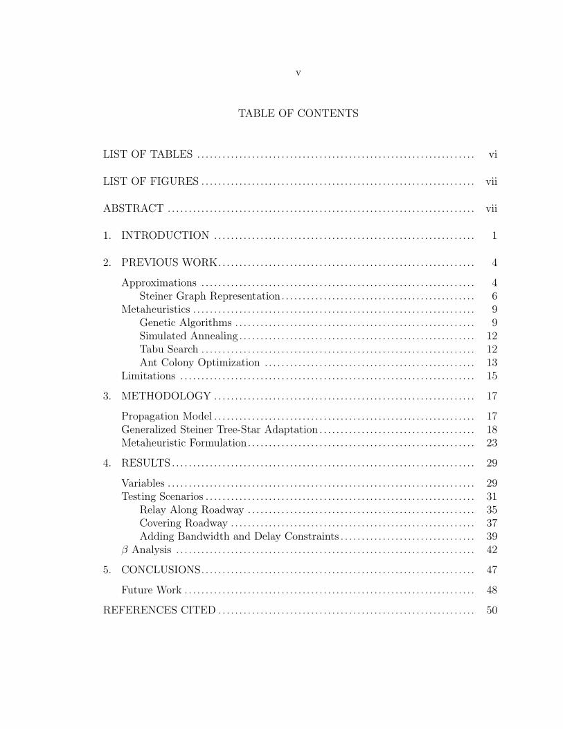
Figure 2 (a) shows an example GSTS graph, where Steiner nodes are hollow
(white) vertexes and terminal, non-Steiner nodes are solid (black) vertexes. In Figure
2 (b), one possible MST solution to the given GSTS example is shown.
(a) (b)
Figure 2. Example GSTS Graph and One MST Solution.
[15] develops an ILP formulation for solving the MST problem in Steiner graphs
with 2|E|+(|V |−1) ILP variables and 4|E|+3|V |+|S|−4 constraints. Their approach
is a solid foundation to solving the MST problem, but they do not develop any
approximations. In addition, their approach does not consider bandwidth, maximum
delay, or redundancy constraints.
[10] develops a 5-approximation algorithm to solve MST in GSTS graphs. They
adapt existing approximations for the uncapacitated facility location (UFL) problem

8
and adapt them to solve the MST problem. Their approach does not consider band-
width, maximum delay, or redundancy constraints, and the approximation bounds
remain large.
[16] develops a 2.5-approximation algorithm for solving the MST problem in
Steiner graphs. They apply the approximation to solving the NDP of selecting relay
nodes in a wireless sensor network. Their approach allows for bounded edge lengths
to maximize network lifetime. However, their approach does not consider bandwidth,
maximum delay, or redundancy constraints, and the approximation bounds remain
large.
[17] solves a variation of the GSTS where connectivity requirements are given
as node pairs (vi, vj, r) instead of the entire MST problem. Similar to [11], each
requirement says that r edge-disjoint paths must exist between vi and vj. They
develop a 2dlog2(rmax + 1)e-approximation where rmax is the highest r constraint.
Their approach does not consider bandwidth or maximum delay constraints, and the
approximation bounds remain large.
[18] develops a 2-approximation for the MST problem in GSTS graphs with the
assumption that all edge and vertex costs are unique. We compare our metaheuristic
against this approximation because it has a low bound while still solving a Steiner
representation of the NDP. Their approach does not consider bandwidth, maximum
delay, or redundancy constraints, and the approximation bounds remain too large to
directly provide a practical solution.

9
[19] develops a 2(1− 1l)-approximation to solving the MST in Steiner graphs where
l is the number of leaves in the optimal tree. In GSTS graphs, the number of leaves is
exactly the number of terminal nodes |{v | v /∈ S}|. Their approach does not consider
bandwidth, maximum delay, or redundancy constraints, and approximation bounds
remain large.
[20] develops a 1.598-approximation algorithm by assuming that the Steiner graph
can be considered complete with new edge weights assigned as the shortest path
length. They use a previous approach [21] in an iterative framework to reach their
bounds. Their assumptions about the behavior of edge weights are reasonable in geo-
metric cases, but these assumptions do not hold for the NDP. Thus this approximation
cannot be used to solve the NDP.
[22] develops a 1 + ln32
-approximation algorithm similar to [20]. Their approach
assumes that edge weights are metric (the triangle inequality holds), which does not
hold for the NDP. Thus this approximation cannot be used to solve the NDP.
Metaheuristics
Metaheuristics are another method of solving NP-complete and NP-hard prob-
lems in polynomial time. The metaheuristics presented here are artificial intelligence
algorithms designed to search for good NDP solutions while meeting constraints.

10
Genetic Algorithms
Genetic algorithms (GAs) are defined using a genetic representation of the prob-
lem space, a fitness function, and crossover and mutation operators. The GA starts
with a random population of solutions and then uses a fitness function to select a
subset for reproduction. The crossover and mutation operators are then applied to
this subset to create a new population of child solutions. This process is then repeated
using the new population as the input. Each step through this process is known as a
generation. The GA repeats this process for several generations until a termination
condition is met.
Several sources have applied GAs to the NDP of selecting tower locations for
cellular networks which are modeled as two-layer networks with the mobile handset
connecting to a local cell and each cell connecting directly to a global backbone.
Redundancy is important in cellular networks so that calls are not dropped as mo-
bile handsets pass between cells. While low delay is important in cellular networks,
maximum delay constraints are not relevant because there are only two layers in the
network.
[7] models the NDP as a minimum dominating set (MDS) problem and solves
it using multiple GA instances running in parallel. They consider bandwidth as the
number of calls that each tower needs to handle, but do not consider redundancy.
Their coverage requirement tries to maximize the ground area covered by towers, and
does not handle explicit coverage constraints.

11
[9] develops a GA to design radio networks using microcells that only cover small
areas. They assume that all bandwidth constraints and node costs are uniform, and
they do not consider redundancy constraints. Similar to [7], they focus simply on
maximizing coverage area.
[23] also addresses the design problem using a GA. They handle coverage con-
straints as reception test points (RTP) which must have signal, service test points
(STP) which must have an acceptable signal-to-noise ratio, and traffic test points
(TTP) which must have a given bandwidth available. They also handle redundancy
by requiring overlap between each cell to facilitate mobile hand-over.
[24] considers the case where cellular towers are already placed. Their approach
designs the wired network from each existing cellular tower back to base station
controllers and mobile switching centers. They also consider the bandwidth require-
ments of each cell. Their approach does not consider redundancy or maximum delay
constraints.
[25] develops a method of finding the Pareto front between cellular coverage and
cost over a region. In the process, they develop a GA to place cellular towers using the
Hata propagation model to validate radio paths. Their approach does not consider
bandwidth, maximum delay, or redundancy constraints.
[26] considers the design of wireless sensor networks. They develop a multiob-
jective GA where the competing objectives are cost and network lifetime based on
battery life, similar to the problem described in [13].

12
Simulated Annealing
Simulated annealing (SA) is a local search technique that uses a single solution to
derive neighboring solutions, and then probabilistically moves toward neighbors with
lower costs. As a SA algorithm progresses, it “cools” which reduces the probability
of selecting a non-optimal neighbor.
[27] develops an SA approach to designing multi-layered telecommunication net-
works using leased wired infrastructure. They consider bandwidth demands of clients
and focus on link pricing based on varying capacity. They also consider redundancy re-
quirements and add additional links between add drop multiplexers (ADM) as needed.
They compare SA results against a LP relaxation and find 33% better results.
[6] develops an SA approach that also finds optimal antenna parameters such as
power, azimuth, and tilt. Their approach focuses on cellular networks and thus designs
only two-layer networks. They address minimizing interference between multiple
sites, and verify that at least one coverage point in each cell has hand-over coverage
provided by four other cells. They consider bandwidth requirements as the number
of simultaneous calls that each cell must handle.
Tabu Search
Tabu search (TS) is a local search technique similar to simulate annealing. It uses
a single solution to derive neighboring solutions, and then probabilistically moves
toward neighbors with lower costs. The algorithm maintains a “tabu” list of all
previously visited solutions to prevent looping and avoid local optima.

13
[3] develops an ILP that solves the two-layer capacitated network design prob-
lem (CNDP). They develop an approximation based on algorithms for solving the
multiple-choice multidimensional knapsack problem (MCMKP). They use a greedy
algorithm to form an initial solution, and then apply TS to find a more optimal so-
lution. While their approach considers bandwidth constraints, it does not consider
maximum delay or redundancy constraints.
[28] models the NDP as a Steiner tree-star graph and solves the MST problem
using TS. In each iteration they swap Steiner nodes to create new solutions from an
existing solution list. The tabu list prevents them from selecting swaps that violate
any solution constraints. Also, after a swap they prevent its reversal for a given num-
ber of generations. They compare their results against a local search heuristic, and
confirm that their TS approach finds the optimal solution for several test cases. Their
approach does not consider bandwidth, maximum delay, or redundancy constraints.
[29] applies TS to find an optimal multicast routing tree while meeting quality-of-
service (QoS) constraints. They consider both bandwidth and delay constraints, and
show that their TS approach performs better than several other heuristics. However,
their approach does not consider redundancy constraints.
Ant Colony Optimization
Ant colony optimization (ACO) models the behavior of real-world ants as they
search for food [30]. As the ants search, they leave a trail of pheromone behind to help
guide future ants towards optimal paths to food. As time progresses, the pheromone

14
on non-optimal paths slowly evaporates while the pheromone on near-optimal paths
is reinforced. Figure 3 illustrates how, after time, pheromone is concentrated (darker)
on a short path around the obstacle, thus influencing more ants to follow that path.
Figure 3. Pheromones on Ant Trails.
In ACO, virtual ants construct solutions by traversing a graph using a local
heuristic and existing pheromones as a guide. Several ants work together to construct
a population of solutions, called a generation. Depending on the ACO variation, ants
deposit pheromone either during or after solution construction. The MAX -MIN
Ant System (MMAS) is one ACO variation that deposits pheromones at the end of
each generation using the best known solution. This construction and update process
is repeated for a set number of generations, or until the pheromones converge.

15
[31] develops an ACO approach for solving the MST problem on traditional
Steiner graphs. They place ants on each terminal node in the Steiner graph. As each
ant moves across the graph, the local heuristic tries to merge towards any nearby
ant trails. Once all ants have merged, the ACO solution is an MST solution. How-
ever, this approach does not consider bandwidth, maximum delay, or redundancy
constraints.
[32] develops an ACO approach to solving the MST problem on rectilinear Steiner
graphs. Rectilinear Steiner graphs are defined in Euclidean space with the constraint
that all edges must be strictly horizontal or vertical. Solutions to this problem are
important to finding optimal wire routing in circuit design. However, because of the
Euclidean constraints this approach cannot be used to solve the NDP.
Limitations
After a survey of the NDP, we found that several approaches have been developed
to find solutions in polynomial time. However, some approaches make assumptions
about circular or uniform radio coverage [16] [12] [7] [26] [9] [33], which do not hold
true over non-trivial distances in rural, mountainous areas.
Other approaches only consider two-layer network designs [3] [6] [7] [23] [9], which
can be infeasible in rural areas where the ability to relay through several layers can
be critical to optimal network design.

16
Only a few algorithms consider bandwidth and redundancy constraints [12] [27]
[11], but even then only in a limited way. In addition, only one algorithm considers
delay constraints [29].
Approximation algorithms exist for the MST problem, but the best applicable
approach is a 2-approximation [18] that does not consider bandwidth, delay, or re-
dundancy constraints.

17
METHODOLOGY
Propagation Model
There are two general methods of computationally determining the feasibility of
a given radio link. One method is to assign each node a radius of communication
based on radio power and antenna gain [2] [16]. This results in a circular coverage
area with the node at the center. A link is considered possible when each node is
within the coverage area of the opposite node. While this method is simple, it does
not accurately model a real-world environment where terrain can drastically change
the coverage area of a given node.
Another method is to examine the terrain along the path between the two nodes.
Several algorithms follow this method, and many radio engineers agree that the Ir-
regular Terrain Model (ITM), also called the Longley-Rice Model, is one of the most
accurate [34]. ITM is based on solid propagation theory and has been well-tested
in various terrain and environmental conditions. The height above average terrain
(HAAT) of the transmitter and receiver sites are important when examining the ter-
rain between two nodes. Higher towers might result in a better first Fresnel zone
clearance, and therefore better received signal strength.
The ITM estimates the expected power loss ITMloss of a radio signal along a given
path. At the transmitter, the equivalent isotropically radiated power (EIRP) is given

18
in dBm (the power ratio in dB referenced to 1mW ) by Equation 3.1, where p is the
transmitter power in watts, and atx is the transmitter antenna gain in dBi.
EIRP = 10 logp
1mW+ atx ( 3.1)
Given a transmitter EIRP and path loss ITMloss, the receiving radio has a sen-
sitivity r given in dBm. This sensitivity indicates the signal strength required to
successfully decode a message from the transmitter. Some radios have multiple band-
widths depending on the received signal strength, as shown later in Table 1 on page
30. Typically a stronger signal will allow for higher bandwidths. Equation 3.2 shows
the relationship that needs to hold for a signal to be decoded at a given receiver with
sensitivity r and antenna gain arx.
EIRP− ITMloss + arx > r ( 3.2)
To best model real-world conditions, our approach uses the ITM to analyze radio
link feasibility. We use 10-meter resolution elevation data to maintain accuracy in
extreme terrain conditions [35]. Because the ITM does not consider foliage, we aug-
ment it with Weissberger’s Modified Exponential Decay Model to estimate path loss
caused by any trees in the radio line-of-sight path [36].

19
Generalized Steiner Tree-Star Adaptation
Similar to [10], we model the network design problem as a generalized Steiner tree-
star (GSTS) graph. A GSTS graph is a graph G = (V, E) with both edge weights wij
and vertex weights wi. A subset S ⊆ V are called Steiner vertices. The GSTS graph
is a natural representation for the NDP, where coverage constraints are represented
by terminal nodes, all considered relay nodes are Steiner nodes, and all considered
links are edges. Any minimum Steiner tree (MST) solution to a GSTS graph directly
identifies the relay nodes and links needed to build the network at an optimal cost.
In our construction, terminal nodes represent all coverage requirements. An ad-
ditional terminal node is added to represent a global backbone. We make the as-
sumption that coverage requirements describe which locations must be connected to
this global backbone. Steiner nodes are inserted for each location where we consider
placing a relay node. Methods for selecting possible relay node locations are described
later. One possible method is to discretize an entire area to obtain a grid of possible
relay nodes.
All nodes and edges are assigned costs, each edge has an available bandwidth and
expected delay assigned. All terminal nodes have both a required bandwidth and
maximum delay assigned.
We formally construct the nodes in the GSTS graph as follows:

20
• We place a single terminal node at the top of the graph to represent the backbone
of the network. It is assigned a zero cost, a zero required bandwidth, and an
infinite maximum delay.
• For each coverage requirement, we place terminal nodes at the bottom of the
graph. Each node is assigned a zero cost, a required bandwidth, and a maximum
delay as specified by any constraints.
• We insert Steiner nodes for each location where we consider placing a relay
node. Each relay node is assigned the cost of preparing that site for use as a
relay. This cost might include baseline equipment or construction of a physical
tower. Each relay node is also assigned a zero required bandwidth and an
infinite maximum delay. Various methods for picking possible relay nodes are
discussed in our results.
Then we add edges to the GSTS graph as follows:
• We add edges for any wired links being considered. Each edge is assigned
the cost of installing and commissioning any required equipment. An available
bandwidth and expected delay are also assigned based on equipment specifica-
tions.
• Similarly, for each radio link being considered, we test its feasibility using the
ITM algorithm. If the link is possible with a given set of radio equipment, we
create an edge between the two nodes. Each edge is assigned the cost of the
21
actual radio equipment needed at both ends of the link. An available bandwidth
and expected delay are also assigned based on equipment specifications.
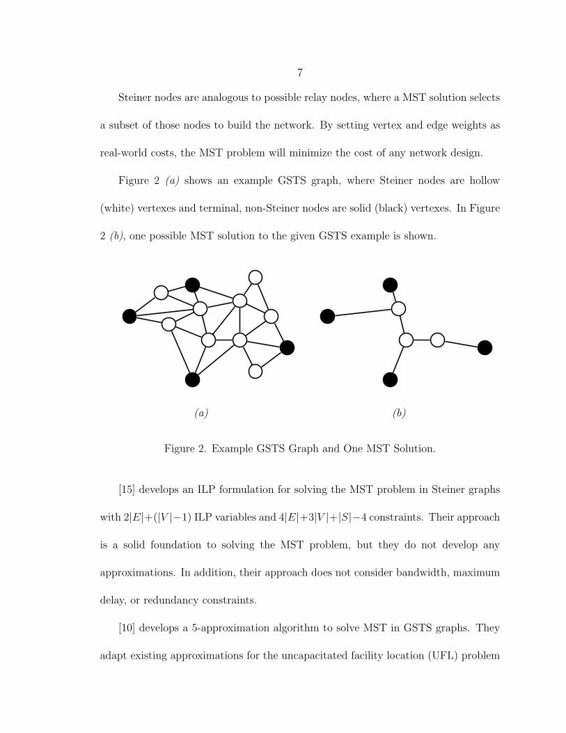
Figure 4 (a) shows an example GSTS graph following the construction outlined
above. Steiner nodes are hollow (white), terminal nodes are solid (black), and con-
sidered links are solid edges. Bandwidth and delay constraints are not shown, and
costs are assumed to be uniform. In Figure 4 (b), one possible MST solution to the
GSTS example is shown.
(a) (b)
Figure 4. Example GSTS Construction Graph and MST Solution.
Additionally, there are some special cases not handled by the above construction:
• When a coverage requirement is defined as a region, we discretize that region
into a set of individual terminal nodes. Any maximum delay constraint is
assigned, in full, to each terminal node. In this thesis we do not consider
bandwidth requirements for regions.

22
• Some wired links may have recurring costs such as line leasing. To consider
this in the network cost, estimate the lifetime of the network design and total
any recurring costs over this lifetime. These total costs can then be applied to
nodes and edges where needed. Advanced pricing techniques, such as equipment
depreciation and net present value, are not considered by this thesis.
• When locations are already developed, or equipment already exists, the assigned
cost can be reduced to reflect this. For example, an existing radio link would
be assigned zero cost while still having an associated available bandwidth and
expected delay.
• Some relay nodes may use a single omnidirectional radio (point-to-multipoint)
to connect with several other nodes. By moving the cost of the omnidirectional
radio to the Steiner node instead of leaving it on each edge, we can ensure that
the overall network cost is calculated correctly. That is, the omnidirectional
radio cost is only counted once when we insert the relay node. Links connected
to an omnidirectional radio often operate in a single, shared channel which can
introduce dynamic changes to available bandwidth and expected delay. In this
thesis we do not model these dynamic changes.
While this construction is similar to previous approaches, it is novel in the way
it distributes real-world costs. The construction also allows for connections to be
relayed through any number of relay nodes before reaching the backbone.

23
Given the construction above, any solution to the MST problem is therefore a
network design meeting all coverage constraints while minimizing cost. Note that the
MST problem does not directly consider bandwidth, maximum delay, or redundancy
constraints. Previous work has developed a 2-approximation algorithm for solving
this MST problem [18]. We next formulate a metaheuristic approach to solving this
MST problem while adding additional functionality to satisfy bandwidth, delay, and
redundancy constraints.
Metaheuristic Formulation
Solving the minimum Steiner tree (MST) problem on GSTS graphs has been
shown to be NP-hard [10]. To solve the problem in polynomial time, we apply an
artificial intelligence metaheuristic called ant colony optimization (ACO) [30]. Specif-
ically, we use the the MAX -MIN Ant System (MMAS) variation of ACO.
Following the approach described in [30] and [37], all pheromones are initialized
to τinit and we construct a population of p MST solutions. Each solution S = (V ′, E ′),
where V ′ ⊆ V and E ′ ⊆ E, is constructed by a unique group of ants. Each population
of solutions is called a single generation. At the end of each generation, we use the
lowest-cost solution found so far to update the pheromones. We repeat this process
for g generations, or until pheromones converge. The final output is the lowest-cost
MST solution found over all generations.

24
For the construction of each solution, one ant will be placed at each terminal node
at the bottom of the graph. Each ant is assigned the bandwidth required by and the
maximum delay constraint of the terminal node it represents. We randomly select
one of those ants to completely traverse the GSTS graph until it reaches the global
backbone terminal node. When this ant is finished, we randomly select the next ant
until all ants all reach the backbone. This random selection of ants is necessary to
counter bias introduced by our serial construction method.
When an ant is selecting the next edge to follow, it considers the lowest cost that
each path offers for reaching the global backbone, in addition to any pheromone left
by previous ants. When at node i, the probability of following an edge to node j is
given by Equation 3.3, where τj is the pheromone value for node j, and ηij is the
local heuristic defined later. α and β are mixing constants defined later.
P (j|i) =ταj ηβ
ij∑(i,k)∈E τα
k ηβik
( 3.3)
We only consider edges in E that both have enough available bandwidth to sup-
port our bandwidth requirement and have an expected delay low enough to not violate
our maximum delay requirement. When we follow an edge, we subtract our required
bandwidth from that edge’s available bandwidth. This ensures that future ants will
not overload an edge’s bandwidth. In addition, when we follow an edge we subtract
its expected delay from our maximum delay requirement. This ensures that data

25
from our terminal node will be able to reach the global backbone within the overall
maximum delay required.
The probability function P (j|i) mixes the pheromone and local heuristic values
using α and β, respectively. These mixing variables control how much we depend on
previous experience versus heuristic knowledge when constructing each solution. In
our results we test various β values and compare their performance.
The local heuristic ηij is dynamic and is computed as shown in Equation 3.4,
where sij is the lowest-cost path from node i to j, node 0 being the backbone terminal
node, V ′ being the set of vertices already selected by other ants, and ε being an
arbitrarily small constant for breaking ties.
ηij =
sij + sj0 if i ∈ V ′ and j ∈ V ′
2× (sij + sj0) if i ∈ V ′ and j /∈ V ′
sij + min{sj0 − ε, mink∈V ′sjk} if i /∈ V ′( 3.4)
Similar to [31], this heuristic tries to merge the ant with any existing nearby ant
trails, otherwise it moves towards the backbone node. Once the ant has merged with
another trail (i ∈ V ′), it is encouraged to move along that existing trail toward the
backbone (j ∈ V ′). If all nodes j ∈ V ′ cannot be followed because of some bandwidth
or delay constraint, then we consider nodes outside of existing trails (j /∈ V ′).
To illustrate this local heuristic, we look at examples of each case described above.
Consider the GSTS graph in Figure 5 (a), where the ant from t3 has already reached
the terminal node t0. We assume that edge and node costs are uniform for this
example. Considering the ant from t1 currently at node a, the third clause of the
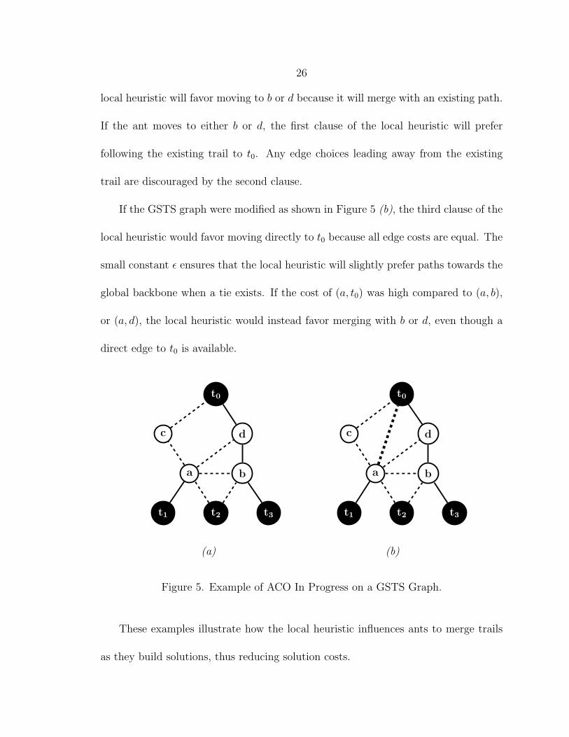
26
local heuristic will favor moving to b or d because it will merge with an existing path.
If the ant moves to either b or d, the first clause of the local heuristic will prefer
following the existing trail to t0. Any edge choices leading away from the existing
trail are discouraged by the second clause.
If the GSTS graph were modified as shown in Figure 5 (b), the third clause of the
local heuristic would favor moving directly to t0 because all edge costs are equal. The
small constant ε ensures that the local heuristic will slightly prefer paths towards the
global backbone when a tie exists. If the cost of (a, t0) was high compared to (a, b),
or (a, d), the local heuristic would instead favor merging with b or d, even though a
direct edge to t0 is available.
t1 t2 t3
t0
a b
c d
t1 t2 t3
t0
a b
c d
(a) (b)
Figure 5. Example of ACO In Progress on a GSTS Graph.
These examples illustrate how the local heuristic influences ants to merge trails
as they build solutions, thus reducing solution costs.

27
As the ant moves through the graph, it maintains a tabu list of edges it has
already visited. While this prevents looping, it can also result in dead-end solutions
where an ant becomes stuck at a node after exhausting all feasible edges leaving the
node. When we find a dead-end solution, we reset the entire solution S = (∅, ∅),
place all ants back on their respective terminal nodes, and start building the solution
again.
Redundancy constraints can be defined as requiring n unique edge-disjoint paths
with an r-edge relaxation. For each additional unique path required, we place another
ant on the terminal node. All ants from a given terminal node use a shared tabu list,
which prevents them from sharing any common edges as they construct paths to the
global backbone. The r-edge relaxation allows ants to ignore this tabu list when they
are less than r edges from reaching the global backbone. Without this relaxation,
there may be no possible solution with n completely unique paths to the backbone.
After generating a population of p solutions, we update the pheromones across the
graph as shown in Equations 3.5 and 3.6 using the lowest-cost solution S∗ = (V ∗, E∗)
found so far, where τiθ is the pheromone for vertex i at generation θ, and ρ is a constant
pheromone evaporation rate. This is based on the pheromone update process for
MMAS [37] [38].
τ ′iθ
=
{τiθ + 1/S∗
cost if i ∈ V ∗
(1− ρ)τiθ if i /∈ V ∗ ( 3.5)

28
τiθ+1= max{τmin, min{τmax, τ
′iθ}} ( 3.6)
This update rule increases the pheromone of any nodes included in the solution S∗,
while exponentially decaying the pheromone of all other nodes. We place pheromones
on nodes instead of edges because solutions do not depend on construction order.
Finally, we enforce a pheromone range [τmin, τmax] before storing the new pheromone
value.
As mentioned above, we repeat the population process until pheromones converge,
or for a constant g generations. It is important to note that pheromone convergence
results in a convergence in value. That is, solutions generated by a set of pheromones
will be similar in cost, but may be very different in construction. We formally define
pheromone convergence below, where ε is a small constant.
{τi ≤ τmin + ε or τi ≥ τmax − ε | ∀ i ∈ V } ( 3.7)
This describes pheromone convergence as the situation where all pheromones have
moved within ε of either the maximum or minimum pheromone value.
29
RESULTS
We tested our metaheuristic approach to solving the network design problem
(NDP) by examining several real-world scenarios and comparing our solutions to a
2-approximation algorithm [18]. For each testing scenario we applied the GSTS con-
struction and ACO algorithm described earlier to find near-optimal NDP solutions.
Because the 2-approximation algorithm requires unique edge and vertex costs [18],
we randomly perturbed the assigned GSTS costs to have a 1% variation.
For testing we implemented both our ACO approach and the 2-approximation
algorithm in C++ on a dual-processor Intel Xeon E5345 computer (eight 2.33GHz
cores in total) with 16GB of RAM. We used Floyd’s algorithm to generate an sij
lookup table, and used modified standard template library (STL) data structures
for storing the GSTS graph and solutions. We used the ITM propagation algorithm
with 10-meter digital elevation model (DEM) data from the United States Geological
Survey (USGS).
It should be noted that any NDP solutions should be reviewed by a professional
radio engineer before actual deployment. This ACO algorithm does not account for
all possible variables, such as radio interference or man-made obstructions. These
variables can be hard to quantify as algorithm inputs, and are left for manual exam-
ination by an engineer.
30
Variables
For our GSTS construction, we assigned real-world costs, available bandwidth,
and expected delay with the guidance of a professional radio engineer. For equipment
we assumed the use of typical 900MHz [39] and 5.8GHz [40] radio systems as shown
in Table 1. As mentioned earlier, the expected bandwidth of a radio link is based on
the sensitivity needed to receive a transmitted signal after considering ITM-estimated
path loss.
The 900MHz system we selected operates in the unlicensed 902-928MHz ISM
(industrial, scientific and medical) band at distances up to 40km. The 5.8GHz system
we selected operates in the 5.725-5.875GHz ISM band at distances up to 80km.
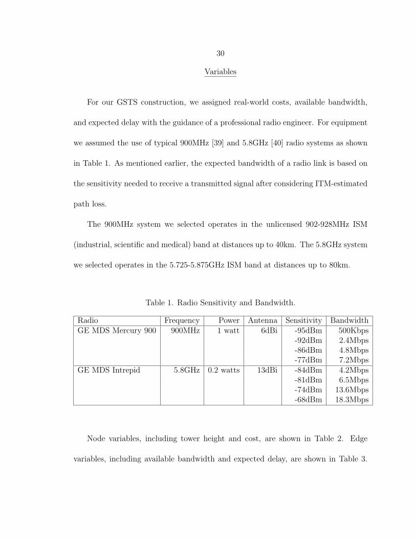
Table 1. Radio Sensitivity and Bandwidth.
Radio Frequency Power Antenna Sensitivity BandwidthGE MDS Mercury 900 900MHz 1 watt 6dBi -95dBm 500Kbps
-92dBm 2.4Mbps-86dBm 4.8Mbps-77dBm 7.2Mbps
GE MDS Intrepid 5.8GHz 0.2 watts 13dBi -84dBm 4.2Mbps-81dBm 6.5Mbps-74dBm 13.6Mbps-68dBm 18.3Mbps
Node variables, including tower height and cost, are shown in Table 2. Edge
variables, including available bandwidth and expected delay, are shown in Table 3.

31
In our construction we select only one receiver sensitivity value for each category of
radio links as shown in Table 3.
Table 2. Assigned GSTS Node Variables.
Type Tower Height CostTerminal node 10m $0Roadside relay node 10m $2,000Existing backbone relay node varies $10,000New backbone relay node 15m $50,000
Table 3. Assigned GSTS Edge Variables.
Type Frequency Bandwidth Delay CostTerminal to Roadside relay 900MHz 500Kbps 10ms $0Roadside relay to Roadside relay 900MHz 2.4Mbps 10ms $1,000Roadside relay to Backbone relay 5.8GHz 6.5Mbps 20ms $5,000Backbone relay to Global backbone wired 10Mbps 30ms $0
For our ACO algorithm we set the parameters α, β, τmin, τmax, and ρ as follows.
Based on the approach in [38], our ACO algorithm uses α = 1, τmin = 2/estimate-opt,
τmax = 5, and ρ = 0.95, where estimate-opt is the solution cost found by the 2-
approximation algorithm. Based on our analysis presented later, we set β = 30. For
pheromone convergence testing, we set ε = 0.01.
For all of our results presented here, we ran the ACO algorithm a constant number
of generations and measured how many generations it took to converge in solution
value.

32
Testing Scenarios
We selected several segments of real-world highways to use as testing scenarios.
Using these scenarios we solved two different NDP variations: one where we relayed
a connection along the highway between two points, and one where we covered the
entire roadway. For our scenarios we selected segments along US-299, US-3, US-199,
US-191, and US-101:
• US-299 runs between Arcata and Redding in northern California. It winds
through mountainous terrain in a rural area, and existing cellular coverage is
sparse. For the US-299 (a) scenario we considered one existing and one new
backbone relay tower. For the US-299 (b) scenario we considered two new
backbone relay towers.
• US-3 runs between Douglas City and Hayfork in northern California. It winds
sharply through mountainous terrain in a rural area, and existing cellular cov-
erage is sparse. For this scenario we considered two new backbone relay towers.
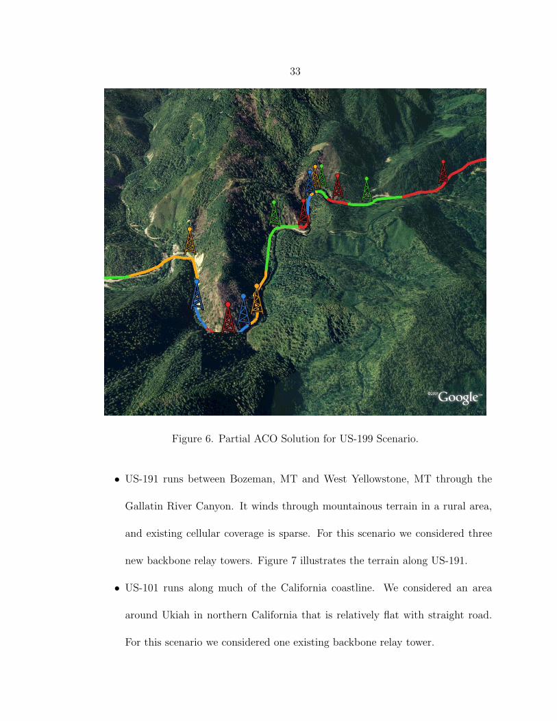
• US-199 runs between Crescent City, CA and Grants Pass, OR through the Smith
River National Recreation Area. It winds sharply through heavily mountainous
terrain in a very rural area, and existing cellular coverage is very sparse. For the
US-199 (a) scenario we considered three existing backbone relay towers. For the
US-199 (b) scenario we considered one existing backbone relay tower. Figure 6
illustrates the terrain along US-199.
33
Figure 6. Partial ACO Solution for US-199 Scenario.
• US-191 runs between Bozeman, MT and West Yellowstone, MT through the
Gallatin River Canyon. It winds through mountainous terrain in a rural area,
and existing cellular coverage is sparse. For this scenario we considered three
new backbone relay towers. Figure 7 illustrates the terrain along US-191.
• US-101 runs along much of the California coastline. We considered an area
around Ukiah in northern California that is relatively flat with straight road.
For this scenario we considered one existing backbone relay tower.

34
Figure 7. Partial ACO Solution for US-191 Scenario.
In our construction we differentiated between three types of relay nodes: roadside
relay nodes, existing backbone relay nodes, and new backbone relay nodes.
• Roadside relay nodes can be placed anywhere along the side of a road. We
consider the center of the road when placing relay nodes. Because the distance
from the road center to either shoulder is about 10 meters, relay towers can be
placed on either side of the road with minimal effect on propagation. However,

35
with this assumption manual verification by an engineer should take place before
actual network deployment.
• Existing backbone relay nodes were selected from a publicly available FCC
database. For our scenarios, we selected only state-owned radio towers above
10 meters in height. Usually these towers have several radios already installed,
and additional radios can be added.
• New backbone relay nodes were considered in areas with few existing backbone
relay nodes. We selected sites on nearby mountain ridges that appeared to have
back-road access.
Different costs are assigned to each of these relay node types as listed in Table 2.
We assume that all backbone relay nodes have direct global backbone connectivity
through existing wired infrastructure.
Relay Along Roadway
First we considered the NDP of relaying a connection along a roadway between
two points x and y. These two points are assumed to be at the roadside. For our
GSTS graph, we inserted both x and y as terminal nodes and considered x to be
our global backbone terminal node. Then we discretized the roadway between the
two points in 25-meter steps. These discretized points became the candidate relay
locations and were inserted into the GSTS graph as Steiner nodes. All terminal and
Steiner nodes were assigned costs as specified in Table 2. No bandwidth, maximum
delay, or redundancy constraints were specified.

36
Then we used the ITM algorithm to test each pair of points in the GSTS graph, in-
serting edges where communication was possible based on the radio parameters given
in Table 1. All edges were assigned costs, available bandwidth, and expected delay
as specified in Table 3. Finally, we ran our ACO algorithm on this graph for 16 gen-
erations of population 64 each. For this specific NDP construction, a known-optimal
solution can be found in polynomial time using Dijkstra’s shortest-path algorithm.
We tested this construction to explicitly show that our ACO algorithm quickly ap-
proaches known optimal solutions.
We solved this NDP construction for scenarios US-191 and US-199 (b). We first
found the optimal NDP solution using Dijkstra’s algorithm, and then ran our ACO
algorithm. A summary of these two scenarios and their results are listed in Table 4.
Table 4. Relay Along Roadway Scenarios.
US-191 US-199Segment length 48km 43.3kmVertices 1921 1732Edges 144,732 52,410Dijkstra cost $83,014 $44,012ACO cost $83,028 $44,015ACO generations 4 10
For the two scenarios tested ACO found solutions very near the known optimal,
within $14 for US-191 and $3 for US-199 (b). These small cost differences compared

37
to Tables 2 and 3 are due to the perturbed GSTS costs. On average, ACO converged
in solution value after 7 generations.
These results show that ACO can quickly find near-optimal solutions to this
variation of the NDP.
Covering Roadway
The second NDP variation we considered was covering an entire segment of road-
way so that a connection to the backbone could be made at any point along the
roadway. This scenario is important for many applications, such as Vehicle Infras-
tructure Integration (VII), roadside assistance, and public safety operations.
For our GSTS graph, we inserted Steiner nodes for any considered backbone
relay nodes. Then we discretized the roadway segment in 25-meter steps. For each
discretized point along the road, we inserted both a terminal and a Steiner node
into the GSTS graph: the terminal node representing the need to cover that point of
roadway, and the Steiner node representing that we are considering placing a roadside
relay at that point. All terminal and Steiner nodes were assigned costs as specified in
Table 2. No bandwidth, maximum delay, or redundancy constraints were specified.
Then we used the ITM algorithm to test each pair of points in the GSTS graph,
inserting edges where communication was possible based on the radio parameters
given in Table 1. All edges were assigned costs, available bandwidth, and expected
delay as specified in Table 3. When running the ITM propagation tests we did not
consider the mobile case where nodes move along the highway.

38
We solved this NDP construction for scenarios US-299 (a), US-299 (b), US-3, US-
199 (b), and US-191. We first ran the 2-approximation algorithm, and then ran our
ACO algorithm for 16 generations of population 64 each. A summary of all tested
scenarios and their results are listed in Table 5. The first section shows statistics
including the road length considered and the number of vertices and edges in the
constructed GSTS graph. The second section shows the running time of the ITM
propagation algorithm and Floyd’s algorithm which are required overhead for both
solution approaches.
The third section shows the running time in seconds taken by each solution ap-
proach. When calculating the total running time of a given approach, the time taken
for both overhead algorithms should also be included. The fourth section shows the
cost of the final solution returned by both algorithms. The final section shows the
number of generations ACO took to converge in solution value.
Table 5. Covering Roadway Scenarios.
US 299 (a) US 299 (b) US 3 US 199 US 191Segment length 16.6km 22.2km 16.5km 12km 39.3kmVertices 1329 1771 1317 956 3140Edges 41,307 375,626 74,301 24,157 225,497
ITM algorithm 24.4s 48.1s 25.2s 13.4s 384.6sFloyd’s algorithm 48.8s 125.2s 48.0s 17.3s 647.0s
2-approximation 5.0s 20.7s 5.8s 2.8s 37.5sACO algorithm 214.1s 422.3s 225.3s 150.8s 763.6sApproximation cost $211,350 $140,770 $194,320 $128,960 $275,146ACO cost $140,350 $126,770 $152,330 $89,970 $236,152
ACO generations 11 13 7 8 2

39
Portions of the ACO solution for the US-199 (b) scenario are shown in Figure 6,
and for the US-191 scenario in Figure 7.
For the five scenarios tested, ACO performed 22% better than the 2-approximation
algorithm on average and 34% better at best when comparing solution costs. ACO
resulted in a total savings of $204,974 when compared against 2-approximation costs.
ACO converged in solution value after 8 generations on average and 13 genera-
tions at worst. Running ACO for more than 16 generations might have found better
solutions, but these results show that good solutions can be found quickly.
While both algorithms run in polynomial time, the actual running time of ACO
was, on average, 35 times longer than the 2-approximation. Comparing the average
benefit $40,994 against the average running time of about 6 minutes, ACO clearly
offers an advantage over the 2-approximation algorithm.
Adding Bandwidth and Delay Constraints
We then modified the roadway-covering NDP described above to have bandwidth
and maximum delay constraints. We tested the extreme case where each discretized
point along the roadway would have a bandwidth requirement of 64kbps and a max-
imum delay requirement of 100ms.
We tested both the US-299 (a) and US-199 (b) scenarios, running ACO for 16
generations of population 64 each. The results are summarized in Table 6.

40
Table 6. Covering Roadway Scenarios with Constraints.
US-299 (a) US-199Original ACO algorithm 214.1s 150.8sConstrained ACO algorithm 393.5s 360.6sOriginal ACO cost $140,350 $89,970Constrained ACO cost $221,380 $120,970ACO generations 9 11
We cannot directly compare constrained ACO results against the 2-approximation
algorithm because it does not consider bandwidth or delay constraints. We mention
our original unconstrained ACO results for reference only.
For the scenarios tested, we see that a constrained ACO algorithm runs about 2
times slower than an unconstrained ACO algorithm. This is because constrained ACO
algorithms are more likely to become trapped in dead-end cases where all edges with
enough available bandwidth have been exhausted (and thus are tabu). As described in
our methodology, solutions are reinitialized to S = (∅, ∅) when they become trapped.
Although we have no direct comparison, we can see that constrained ACO so-
lutions are still near the costs of the unconstrained ACO and 2-approximation al-
gorithms. The constrained ACO algorithm converges in solution value after 10 gen-
erations on average, compared to 8 generations average for the unconstrained ACO
algorithm.
Figure 8 shows the MST solution selected by the unconstrained ACO algorithm
for the US-199 (b) scenario, and Figure 9 shows the MST solution selected by the

41
constrained ACO algorithm for the same scenario. Four layers are shown in each
figure, the top layer containing the single global backbone, the second layer of selected
backbone relays, the third layer of selected roadside relay nodes, and the fourth layer
of all terminal nodes along the roadway.
Figure 8. Unconstrained MST Solution.
Figure 9. Constrained MST Solution.
We can see in Figure 9 that the constrained ACO algorithm is forced to include
more routes as it works towards the global backbone at the top of the GSTS graph. In
the constrained MST solution, bandwidth aggregates as ants make their way towards

42
the global backbone. As the bandwidth is exhausted from previously selected links,
ants select other links that allow them to still reach the global backbone.
The unconstrained MST solution only selects two radio links from roadside relays
to a single backbone relay. In Figure 9 the constrained ACO algorithm selects one
additional backbone relay and two additional links from the roadside to the backbone.
In addition, much of the roadside relay structure is reorganized to distribute traffic
loads without violating bandwidth constraints.
These additional links allow the solution to meet the bandwidth and delay con-
straints while still minimizing network cost. In both scenarios our ACO approach
quickly converges in value to solutions that are similar in cost to those found by the
unconstrained ACO algorithm. This shows that the ACO approach can meet added
constraints with minimal cost increase.
β Analysis
One important variable of our ACO algorithm is β which weights our local heuris-
tic. Optimal β values will help ACO find good solutions quickly, while non-optimal
values will increase the time needed to find good solutions. Setting β = 0 is equivalent
to a random search without heuristic guidance. In this section we present extensive
testing of various β values before selecting β = 30.
For the roadway-covering NDP described earlier we tested four scenarios US-199
(a), US-199 (b), US-191, and US-101. For each scenario, we independently tested

43
discrete β values in the range [1,120]. For each β tested, we ran our ACO algorithm
15 times and compared the average solution cost against the 2-approximation algo-
rithm. Each ACO run is different due to the randomness involved. Because β is not
a parameter for the 2-approximation algorithm, there is only one 2-approximation
solution for each scenario.
Below we present each of the four scenarios, showing the average ACO solution
cost with standard deviation. The left axis is the solution cost in thousands of dollars,
and the right axis is the average number of generations that each ACO run took to
converge in solution value.
50
60
70
80
90
100
110
120
10 1000
4
8
12
16
Solution cost Generations
β
ACO cost
3333
3
33
33333
3 3 3 3 3
32-approximation cost
ACO generations++
+
+
+
+
++
+++
++
+
++
+
+
Figure 10. β Analysis for US-199 (a) Scenario.

44
90
100
110
120
130
140
150
160
170
180
190
10 1000
4
8
12
16
Solution cost Generations
β
ACO cost33
3
3
33
33
333
3 3 3 3 3
32-approximation cost
ACO generations
+++ + + + +++
+
++
++
+
+
+
Figure 11. β Analysis for US-199 (b) Scenario.
100
120
140
160
180
200
220
240
260
10 1000
4
8
12
16
Solution cost Generations
β
ACO cost
33
3
3
3
3
33333
3 3 3 3 3
32-approximation cost
ACO generations+++
+ + ++++
++
+
+
+
++
+
Figure 12. β Analysis for US-191 Scenario.

45
45
50
55
60
65
70
75
10 1000
4
8
12
16
Solution cost Generations
β
ACO cost
333
3
3
333
3333 3 3 3 3
32-approximation cost
ACO generations++
+ +
+
++++
++
++
+ + +
+
Figure 13. β Analysis for US-101 Scenario.
In Figures 10, 11, 12, and 13 we see that higher β values consistently lead to
better ACO solutions. Beyond β = 20 we see little improvement in solution quality.
When comparing average generations to convergence in solution value, we see
that higher β values tend to converge faster. However, in Figures 11 and 12 we see
that β = 120 takes more generations on average to converge than lower β values.
We conclude that β values beyond 30 offer little improvement to solution quality.
However, no solid conclusions about generations to convergence can be drawn from
this analysis. We see in each scenario that β = 30 offers good solution quality in an
acceptable number of generations. Therefore, we use β = 30 for our ACO algorithm.
46
As we add more bandwidth, maximum delay, or redundancy constraints we would
expect to see lower β values perform better. With more constraints, the shorter paths
favored by the local heuristic have a higher probability of violating a constraint.
Putting less weight on the local heuristic would give ants more freedom to explore
other paths.

47
CONCLUSIONS
In this thesis we developed a generalized Steiner tree-star (GSTS) construction
for solving the network design problem (NDP). We then developed an ant colony
optimization (ACO) approach to solving the minimum Steiner tree (MST) problem
on this GSTS graph while meeting a wide range of constraints including coverage,
bandwidth, delay, and redundancy. This is the first approach to date that considers
all of these constrains simultaneously while minimizing network cost.
We tested our GSTS construction and ACO algorithm using several real-world
scenarios. Our approach quickly found near-optimal solutions for the two relay-along-
roadway NDP scenarios when compared directly with known optimal solutions.
For the five roadway-covering NDP scenarios, our ACO approach performed 22%
($40,994) better, on average, compared to the 2-approximation algorithm with a
running time of under 15 minutes in each case. Our approach converged in solution
value after 8 generations on average. Running ACO for more than 16 generations
might find better solutions, but our results show that relatively good solutions are
found quickly.
When applying bandwidth and maximum delay constraints to two roadway-
covering NDP scenarios, our ACO approach finds solutions near the cost of the uncon-
strained NDP. No direct comparison can be made to the 2-approximation algorithm
because it does not consider bandwidth or maximum delay constraints.

48
We investigated the impact of β on our metaheuristic formulation, and found that
β = 30 offers good solution quality in an acceptable number of generations. β values
above 30 offer only minimal quality improvement.
This thesis shows that our GSTS construction and ACO approach can find near-
optimal NDP solutions in polynomial time. In addition, our approach is the first
to simultaneously consider coverage, bandwidth, maximum delay, and redundancy
constraints.
Future Work
Future work should compare ACO solutions against networks designed by human
engineers. This will give another measure of the benefit offered by our ACO approach
in addition to the 2-approximation algorithm presented here.
Radio engineers often work to maximize the margin between receiver sensitivity
and signal power, represented in Equation 3.2. Larger margins make radio links
more robust when faced with interference not considered by the ITM propagation
algorithm. Our ACO approach could reach this goal by modifying the local heuristic
to prefer links with higher margins.
The approach developed in this thesis only considers the case where one set of
radio equipment (a single edge) is considered between two nodes. With further de-
velopment of the local heuristic and changes to the pheromone update process, we
could consider multiple radio systems (multiple edges) between two nodes. We would

49
expect an ant to follow the edge that best meets the constraints it represents. This
approach would also benefit from local search, where we might exchange multiple
edges between two nodes with a single edge, thus reducing cost while still meeting
constraints.
The α parameter is important when mixing pheromones with the local heuristic,
and it can impact solution quality as generations progress. An analysis of α values
should be performed similar to the β analysis presented in this thesis. An optimal
α value would exploit pheromone knowledge to find better solutions while avoiding
local optima.
Additional β parameter testing should look at its behavior as constraints are
added. In these cases we expect to find that lower β values lead to better solutions.
The network routing problem (NRP) searches for optimal routes through an ex-
isting network while considering available links and bandwidth requirements. These
routes are then used to deliver traffic across the network. Because our approach con-
siders static bandwidth requirements, the routes chosen by our ants could be used as
initial static routes in a dynamic NRP algorithm. Other work has already applied
ACO to solve the dynamic NRP [41] [42].

50
REFERENCES CITED
[1] F. Ikegami, S. Yoshida, T. Takeuchi, and M. Umehira. Propagation factors con-trolling mean field strength on urban streets. IEEE Transactions on Antennasand Propagation, 32:822–829, 1984.
[2] R. Kahn. The organization of computer resources into a packet radio network.IEEE Transactions on Communications, 25(1):169–178, 1977.
[3] B. Lardeux, A. Knippel, and J. Geffard. Efficient algorithms for solving the 2-layered network design problem. In Proceedings of the International NetworkOptimization Conference, pages 367–372, 2003.
[4] A. Markopoulou, F. Tobagi, and M. Karam. Assessment of VoIP quality overinternet backbones. In Proceedings of the Joint Conference of the IEEE Com-puter and Communications Societies, pages 150–159, 2002.
[5] M. Goemans and D. Bertsimas. Survivable networks, linear programming relax-ations and the parsimonious property. Mathematical Programming, 60:145–166, 1993.
[6] S.M. Allen, S. Hurley, and R.M. Whitaker. Automated decision technology fornetwork design in cellular communication systems. In Proceedings of theHawaii International Conference on System Sciences, 2002.
[7] P. Calegari, F. Guidec, P. Kuonen, and D. Wagner. Genetic approach to radionetwork optimization for mobile systems. In Proceedings of the VehicularTechnology Conference, volume 2, pages 755–759, 1997.
[8] J. Sharkey and D. Galarus. Radio network design for rural intelligent transporta-tion systems using artificial intelligence. In Proceedings of the TransportationResearch Board Annual Meeting, 2008.
[9] P. Calegari, F. Guidec, P. Kuonen, B. Chamaret, S. Udeba, S. Josselin, andD. Wagner. Radio network planning with combinatorial optimisation algo-rithms. ACTS Mobile Communications, pages 707–713, 1996.
[10] S. Khuller and A. Zhu. The general steiner tree-star problem. InformationProcessing Letters, 84:215–220, 2002.

51
[11] M. Goemans, A. Goldberg, S. Plotkin, D. Shmoys, E. Tardos, and D. Williamson.Improved approximation algorithms for network design problems. In Proceed-ings of the ACM-SIAM Symposium on Discrete Algorithms, pages 223–232,1994.
[12] B. Hao, H. Tang, and G. Xue. Fault-tolerant relay node placement in wirelesssensor networks: formulation and approximation. Workshop on High Perfor-mance Switching and Routing, pages 246–250, 2004.
[13] J. Tang, B. Hao, and A. Sen. Relay node placement in large scale wireless sensornetworks. Computer Communications, 29(4):490–501, 2006.
[14] S. Bhatnagar, S. Ganguly, and R. Izmailov. Design of IEEE 802.16-based multi-hop wireless backhaul networks. In Proceedings of the International Confer-ence on Access Networks, page 5, 2006.
[15] M. Diane and J. Plesnık. An integer programming formulation of the steinerproblem in graphs. Mathematical Methods of Operations Research, 37(1):107–111, 1993.
[16] X. Cheng, D.Z. Du, L. Wang, and B. Xu. Relay sensor placement in wirelesssensor networks. Wireless Networks, 2007.
[17] A. Agrawal, P. Klein, and R. Ravi. When trees collide: an approximation algo-rithm for the generalized steiner problem on networks. pages 134–144, 1991.
[18] H. Takahashi and A. Matsuyama. An approximate solution for the steiner prob-lem in graphs. Math. Jap., 24:573–577, 1980.
[19] L. Kou, G. Markowsky, and L. Berman. A fast algorithm for steiner trees. ActaInformatica, 15:141–145, 1981.
[20] S. Hougardy and H.J. Promel. A 1.598 approximation algorithm for the steinerproblem in graphs. In Proceedings of the ACM-SIAM Symposium on DiscreteAlgorithms, pages 448–453, 1999.
[21] M. Karpinski and A. Zelikovsky. New approximation algorithms for the steinertree problems. Electronic Colloquium on Computational Complexity, 2(30),1995.
[22] G. Robins and A. Zelikovsky. Improved steiner tree approximation in graphs.In Proceedings of the ACM-SIAM Symposium on Discrete Algorithms, pages770–779, 2000.

52
[23] H. Meunier, E.G. Talbi, and P. Reininger. A multiobjective genetic algorithm forradio network optimization. In Proceedings of the Congress on EvolutionaryComputation, volume 1, pages 317–324, 2000.
[24] M. Shahbaz. Fixed network design of cellular mobile communication networksusing genetic algorithms. In Proceedings of the International Conference onUniversal Personal Communications, pages 163–167, 1995.
[25] R.M. Whitaker, L. Raisanen, and S. Hurley. A model for conflict resolutionbetween coverage and cost in cellular wireless networks. In Proceedings of theHawaii International Conference on System Sciences, 2004.
[26] D. Jourdan and O. de Weck. Layout optimization for a wireless sensor networkusing a multi-objective genetic algorithm. In Proceedings of the VehicularTechnology Conference, volume 5, pages 2466–2470, 2004.
[27] S. Soni, S. Narasimhan, and L.J. LeBlanc. Telecommunication access network de-sign with reliability constraints. IEEE Transactions on Reliability, 53(4):532–541, 2004.
[28] J. Xu, S. Chiu, and F. Glover. Using tabu search to solve the steiner tree-starproblem in telecommunications network design. Telecommunication Systems,6(1):117–125, 1996.
[29] N. Ghaboosi and A. Haghighat. A tabu search based algorithm for multicastrouting with QoS constraints. In Proceedings of the International Conferenceon Information Technology, pages 33–39, 2006.
[30] M. Dorigo and T. Stutzle. Ant Colony Optimization. Bradford Book, 2004.
[31] S. Gosavi, S. Das, S. Vaze, G. Singh, and E. Buehler. Obtaining subtrees fromgraphs: an ant colony approach. In Proceedings of the Swarm IntelligenceSymposium, pages 160–166, 2003.
[32] Y. Hu, T. Jing, X. Hong, Z. Feng, X. Hu, and G. Yan. An efficient rectilinearsteiner minimum tree algorithm based on ant colony optimization. In Pro-ceedings of the International Conference on Communications, Circuits andSystems, volume 2, pages 1276–1280, 2004.
[33] Y. Xin, T. Guven, and M. Shayman. Topology design for wireless ad-hoc net-works with backbone support. In Proceedings of the Conference on Informa-tion Sciences and Systems, 2005.

53
[34] N. De Minco and C. Holloway. Propagation modeling for its applications inthe roadway environment. Journal of Intelligent Transportation Systems,3(4):287–331, 1997.
[35] S. Rose. The effect of digital elevation model resolution on wave propagationpredictions at 24GHz. Master’s thesis, Virginia Polytechnic Institute andState University, 2001.
[36] M. Al-Nuaimi and A. Hammoudeh. Measurements and predictions of attenuationand scatter of microwave signals by trees. In Proceedings of IEE Microwaves,Antennas and Propagation, volume 141, pages 70–76, 1994.
[37] T. Stutzle and H. Hoos. Improvements on the ant system: Introducing max-min ant system. In Proceedings of the International Conference on ArtificialNeural Networks and Genetic Algorithms, pages 245–249, 1997.
[38] T. Stutzle and H. Hoos. The max-min ant system and local search for combina-torial optimization problems. In Proceedings of the International Conferenceon Metaheuristics, pages 313–329, 1999.
[39] GE MDS. MDS Mercury 900 data sheet.
[40] GE MDS. MDS Intrepid data sheet.
[41] M. Gunes, U. Sorges, and I. Bouazizi. Ara-the ant-colony based routing algorithmfor MANETs. In Proceedings of the International Conference on ParallelProcessing, pages 79–85, 2002.
[42] G. Di Caro and M. Dorigo. Antnet: Distributed stigmergetic control for com-munications networks. Journal of Artificial Intelligence Research, 9:317–365,1998.