Automatic segmentation of seven retinal layers in SDOCT images congruent with expert manual segmentation

Automatic segmentation of seven retinal layers in SDOCT images congruent with expert manual

segmentation

Stephanie J. Chiu,1,*

Xiao T. Li,1 Peter Nicholas,

2

Cynthia A. Toth,2,1

Joseph A. Izatt,1,2

and Sina Farsiu2,1

1Department of Biomedical Engineering, Duke University, Durham, NC, 27708, USA

2Department of Ophthalmology, Duke University Medical Center, Durham, NC, 27710, USA *[email protected]

Abstract: Segmentation of anatomical and pathological structures in ophthalmic images is crucial for the diagnosis and study of ocular diseases. However, manual segmentation is often a time-consuming and subjective process. This paper presents an automatic approach for segmenting retinal layers in Spectral Domain Optical Coherence Tomography images using graph theory and dynamic programming. Results show that this method accurately segments eight retinal layer boundaries in normal adult eyes more closely to an expert grader as compared to a second expert grader.

©2010 Optical Society of America

OCIS codes: (100.0100) Image processing; (100.2960) Image analysis; (110.4500) Optical coherence tomography; (170.4470) Ophthalmology.

References and links

1. D. Huang, E. A. Swanson, C. P. Lin, J. S. Schuman, W. G. Stinson, W. Chang, M. R. Hee, T. Flotte, K. Gregory, C. A. Puliafito, and et, “Optical coherence tomography,” Science 254(5035), 1178–1181 (1991).

2. J. G. Fujimoto, W. Drexler, J. S. Schuman, and C. K. Hitzenberger, “Optical Coherence Tomography (OCT) in ophthalmology: introduction,” Opt. Express 17(5), 3978–3979 (2009).

3. I. C. Han and G. J. Jaffe, “Evaluation of Artifacts Associated with Macular Spectral-Domain Optical Coherence Tomography,” Ophthalmology 117, 1177–1189. (2010).

4. S. G. Schuman, A. F. Koreishi, S. Farsiu, S. Jung, J. A. Izatt, and C. A. Toth, “Photoreceptor Layer Thinning over Drusen in Eyes with Age-Related Macular Degeneration Imaged In Vivo with Spectral-Domain Optical Coherence Tomography,” Ophthalmology 116, 488–496 (2009).

5. D. Cabrera Fernández, H. M. Salinas, and C. A. Puliafito, “Automated detection of retinal layer structures on optical coherence tomography images,” Opt. Express 13(25), 10200–10216 (2005).

6. H. Ishikawa, D. M. Stein, G. Wollstein, S. Beaton, J. G. Fujimoto, and J. S. Schuman, “Macular segmentation with optical coherence tomography,” Invest. Ophthalmol. Vis. Sci. 46(6), 2012–2017 (2005).

7. T. Fabritius, S. Makita, M. Miura, R. Myllylä, and Y. Yasuno, “Automated segmentation of the macula by optical coherence tomography,” Opt. Express 17(18), 15659–15669 (2009).

8. A. Yazdanpanah, G. Hamarneh, B. Smith, and M. Sarunic, “Intra-retinal Layer Segmentation in Optical Coherence Tomography Using an Active Contour Approach,” in Proceedings of the 12th International Conference on Medical Image Computing and Computer-Assisted Intervention: Part II, (Springer-Verlag, London, UK, 2009), pp. 649–656.

9. S. Farsiu, S. J. Chiu, J. A. Izatt, and C. A. Toth, “Optical coherence tomography,” Proc. SPIE 6844, 68440D (2008).

10. A. Mishra, A. Wong, K. Bizheva, and D. A. Clausi, “Intra-retinal layer segmentation in optical coherence tomography images,” Opt. Express 17(26), 23719–23728 (2009).

11. M. Haeker, M. Sonka, R. Kardon, V. A. Shah, X. Wu, and M. D. Abramoff, “Automated segmentation of intraretinal layers from macular optical coherence tomography images,” Proc. SPIE 6512, 651214 (2007).

12. M. K. Garvin, M. D. Abràmoff, X. Wu, S. R. Russell, T. L. Burns, and M. Sonka, “Automated 3-D intraretinal layer segmentation of macular spectral-domain optical coherence tomography images,” IEEE Trans. Med. Imaging 28(9), 1436–1447 (2009).

13. K. Lee, M. Niemeijer, M. K. Garvin, Y. H. Kwon, M. Sonka, and M. D. Abramoff, “Segmentation of the optic disc in 3-D OCT scans of the optic nerve head,” IEEE Trans. Med. Imaging 29(1), 159–168 (2010).

14. D. A. Tolliver, I. Koutis, H. Ishikawa, J. S. Schuman, and G. L. Miller, “Automatic Multiple Retinal Layer Segmentation in Spectral Domain OCT Scans via Spectral Rounding,” Invest. Ophthalmol. Vis. Sci. 49, 1878- (2008).

15. E. W. Dijkstra, “A note on two problems in connexion with graphs,” Numerische Mathematik 1(1), 269–271 (1959).

#131667 - $15.00 USD Received 15 Jul 2010; revised 18 Aug 2010; accepted 19 Aug 2010; published 27 Aug 2010(C) 2010 OSA 30 August 2010 / Vol. 18, No. 18 / OPTICS EXPRESS 19413

16. M. Niemeijer, M. K. Garvin, B. van Ginneken, M. Sonka, and M. D. Abramoff, “Vessel segmentation in 3D spectral OCT scans of the retina,” Proc. SPIE 6914, 69148 (2008).

17. J. Shi, and J. Malik, “Normalized Cuts and Image Segmentation,” IEEE Trans. Pattern Anal. Mach. Intell. 22(8), 888–905 (2000).

18. P. Elias, A. Feinstein, and C. Shannon, “A note on the maximum flow through a network,” IRE Trans. Inf. Theory 2(4), 117–119 (1956).

19. S. Warshall, “A Theorem on Boolean Matrices,” J. ACM 9(1), 11–12 (1962). 20. R. Bellman, “On a Routing Problem,” Q. Appl. Math. 16, 87–90 (1958). 21. L. R. Ford, and D. R. Fulkerson, Flows in networks, (Princeton University Press, Princeton, N.J., 1962). 22. R. W. Floyd, “Algorithm 97: Shortest path,” Commun. ACM 5(6), 345 (1962). 23. N. Otsu, “Threshold Selection Method from Gray-Level Histograms,” IEEE Trans. Syst. Man Cyber. 9(1), 62–66

(1979). 24. R. C. Gonzalez, and R. E. Woods, Digital image processing, 3rd ed. (Pearson/Prentice Hall, Upper Saddle River,

NJ, 2008), pp. xxii, 954 p. 25. S. Lu, C. Cheung, J. Liu, J. Lim, C. Leung, and T. Wong, “Automated Layer Segmentation of Optical Coherence

Tomography Images,” IEEE Trans. Biomed. Eng. (to be published). 26. Age-Related Eye Disease Study Research Group, “The Age-Related Eye Disease Study system for classifying

age-related macular degeneration from stereoscopic color fundus photographs: the Age-Related Eye Disease Study Report Number 6,” Am. J. Ophthalmol. 132(5), 668–681 (2001).

27. H. Takeda, S. Farsiu, and P. Milanfar, “Kernel regression for image processing and reconstruction,” IEEE Trans. Image Process. 16(2), 349–366 (2007).

1. Introduction

Accurate detection of anatomical and pathological structures in Spectral Domain Optical Coherence Tomography (SDOCT) images is critical for the diagnosis and study of ocular diseases [1,2]. Commercial OCT systems are equipped with segmentation software mainly targeted to measure the nerve fiber layer and the total retinal thicknesses, with varying rates of success [3]. As for the other ocular features of interest, such as the photoreceptor layer thickness, quantitative data is primarily obtained by manual segmentation [4]. Manual segmentation is not only demanding for expert graders, but is also extremely time-consuming for clinical use, or for large scale, multi-center trials. Furthermore, the inherent variability between graders yields subjective results.

This paper presents a fully automatic approach for segmenting layered structures in ocular images using graph theory and dynamic programming that significantly reduces the processing time required for image segmentation and feature extraction. While the proposed technique can be generalized for segmenting any layered structure in images of any imaging modality, we focus on the segmentation of retinal layers in SDOCT images. Figure 1 shows a cross-sectional SDOCT image of the retina centered at the macula, annotated with the targeted eight layer boundaries delineated by a consensus of the expert graders advising this study (see Section 4.1). Knowledge of these layer boundary positions allows for retinal layer thickness calculations, which are imperative for the study and detection of ocular diseases.

Fig. 1. Target retinal layers of a cross-sectional SDOCT image (B-scan) centered at the macula.


Previous reports have addressed different approaches to segmenting retinal layer boundaries with varying levels of success. Fernández proposed a combined structure tensor and complex diffusion filtering methodology in place of traditional thresholding [5]. Ishikawa implemented a column-wise intensity profiling system for layer classification with mean filtering techniques for de-speckling [6], and Fabritius introduced an alternative method for segmenting the ILM and RPE based on pixel intensity variations [7]. Active contours were yet another method explored by Yazdanpanah for layer segmentation of rodent images [8] and by Farsiu for the segmentation of drusen [9]. Mishra extended the traditional active contour with a two-step kernel-based optimization scheme [10].

Graph-cut segmentation is a technique that has proven to be successful in a variety of medical image segmentation applications; however it has only very recently been introduced into ophthalmic SDOCT segmentation applications. Haeker / Garvin utilized radial scans to generate a composite 3-D image and performed a 3-D graph search of the retinal layers [11,12], and Lee used multi-scale, 3-D graph search for segmenting the optic nerve head [13]. Finally, Tolliver employed the spectral rounding solution of the grouping problem to effectively segment layers in a rather mathematically complex framework [14]. This paper presents a conceptually simpler, yet accurate, alternative approach to graph-cut segmentation using dynamic programming [15].

Our simple algorithmic framework enables us to effectively address previous sources of instability including the merging of layers at the fovea [5,8], uneven tissue reflectivity [6], and the presence of pathology [5]. Moreover, special handling is included for issues such as vessel hypo-reflectivity, where structural information is lost due to shadowing of the vessels. Although previous works address automatic vessel detection [16], we incorporate a simple vessel detection algorithm for more accurate segmentation results. Furthermore, our algorithm is an adaptable framework for images with pathology such as drusen, as well as pediatric and corneal images, among others. Finally, while many successful segmentation techniques rely on volumetric data to accurately segment anatomic structures (e.g [12,13].), our algorithm is able to accurately segment features of interest in individual B-scans, which is important when volumetric data is not available.

The organization of this paper is as follows. Section 2 discusses the general theory behind graph segmentation as well as our generalized method for automatically segmenting layered structures, and Section 3 shows an implementation of the algorithm for segmenting eight retinal layer boundaries in normal adult eyes. Section 4 compares our automated results against expert manual segmentation, and shows the algorithm applied to other types of images such as retinal pediatric and pathological eyes, as well as the cornea.

2. A generalized layer segmentation algorithm

This section proposes a generalized method for segmenting layered structures. We describe the high-level issues when implementing a graph-based segmentation algorithm and describe our proposed solutions. Later, in Section 3, we describe the algorithmic implementation of these solutions in detail for segmenting retinal layers in SDOCT images. The following schematic (Fig. 2) outlines the core steps in our layer segmentation algorithm, which are discussed in the following subsections.

Fig. 2. A generalized layer segmentation algorithm schematic.


2.1 Graph representation and weight calculation

We represent each image (e.g. an SDOCT B-scan) as a graph of nodes, where each node corresponds to a pixel. The links connecting the nodes are called edges. A set of connected edges form a pathway for one to travel across the graph. Weights can be assigned to individual edges to create path preferences. To travel across the graph from a start node to an end node, the preferred path is the route in which the total weight sum is at a minimum. This resulting path is the cut which segments one region from another. For our problem, boundaries between retinal layers correspond to the preferred paths (cuts) on an SDOCT B-scan.

The key to accurately cutting a graph is to assign the appropriate edge weights. Common metrics for varying weight values include functions of distances between pixels or differences between intensity values [17]. As long as the feature to be segmented has characteristics unique to its surroundings, low weights can be assigned to the borders of that feature to distinguish it from the rest of the image.

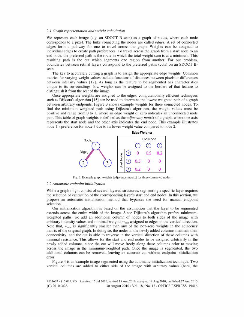
Once appropriate weights are assigned to the edges, computationally efficient techniques such as Dijkstra's algorithm [15] can be used to determine the lowest weighted path of a graph between arbitrary endpoints. Figure 3 shows example weights for three connected nodes. To find the minimum weighted path using Dijkstra's algorithm, the weight values must be positive and range from 0 to 1, where an edge weight of zero indicates an unconnected node pair. This table of graph weights is defined as the adjacency matrix of a graph, where one axis represents the start node and the other axis indicates the end node. This example illustrates node 1’s preference for node 3 due to its lower weight value compared to node 2.

Fig. 3. Example graph weights (adjacency matrix) for three connected nodes.

2.2 Automatic endpoint initialization

While a graph might consist of several layered structures, segmenting a specific layer requires the selection or estimation of the corresponding layer’s start and end nodes. In this section, we propose an automatic initialization method that bypasses the need for manual endpoint selection.

Our initialization algorithm is based on the assumption that the layer to be segmented extends across the entire width of the image. Since Dijkstra’s algorithm prefers minimum-weighted paths, we add an additional column of nodes to both sides of the image with arbitrary intensity values and minimal weights wmin assigned to edges in the vertical direction. Note that, wmin is significantly smaller than any of the non-zero weights in the adjacency matrix of the original graph. In doing so, the nodes in the newly added columns maintain their connectivity, and the cut is able to traverse in the vertical direction of these columns with minimal resistance. This allows for the start and end nodes to be assigned arbitrarily in the newly added columns, since the cut will move freely along these columns prior to moving across the image in the minimum-weighted path. Once the image is segmented, the two additional columns can be removed, leaving an accurate cut without endpoint initialization error.

Figure 4 is an example image segmented using the automatic initialization technique. Two vertical columns are added to either side of the image with arbitrary values (here, the


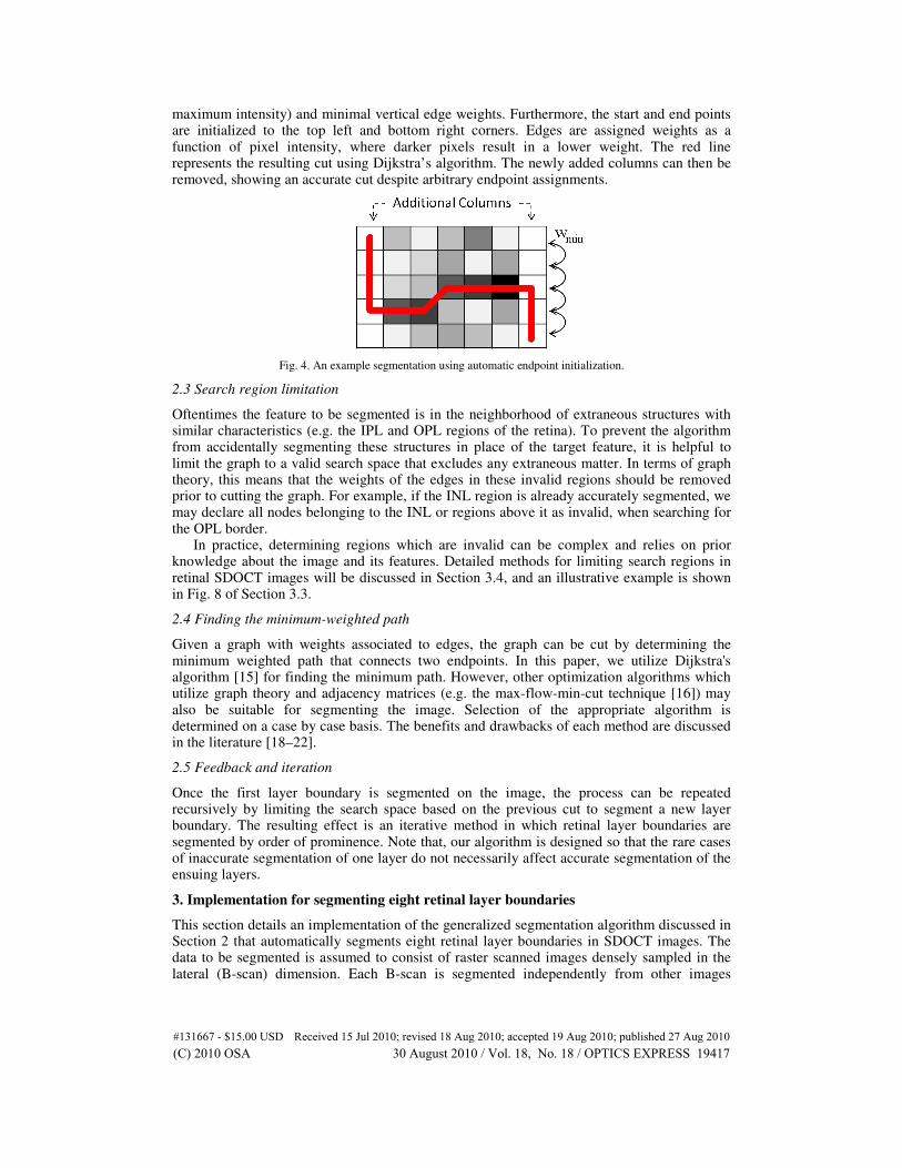
maximum intensity) and minimal vertical edge weights. Furthermore, the start and end points are initialized to the top left and bottom right corners. Edges are assigned weights as a function of pixel intensity, where darker pixels result in a lower weight. The red line represents the resulting cut using Dijkstra’s algorithm. The newly added columns can then be removed, showing an accurate cut despite arbitrary endpoint assignments.

Fig. 4. An example segmentation using automatic endpoint initialization.

2.3 Search region limitation

Oftentimes the feature to be segmented is in the neighborhood of extraneous structures with similar characteristics (e.g. the IPL and OPL regions of the retina). To prevent the algorithm from accidentally segmenting these structures in place of the target feature, it is helpful to limit the graph to a valid search space that excludes any extraneous matter. In terms of graph theory, this means that the weights of the edges in these invalid regions should be removed prior to cutting the graph. For example, if the INL region is already accurately segmented, we may declare all nodes belonging to the INL or regions above it as invalid, when searching for the OPL border.

In practice, determining regions which are invalid can be complex and relies on prior knowledge about the image and its features. Detailed methods for limiting search regions in retinal SDOCT images will be discussed in Section 3.4, and an illustrative example is shown in Fig. 8 of Section 3.3.

2.4 Finding the minimum-weighted path

Given a graph with weights associated to edges, the graph can be cut by determining the minimum weighted path that connects two endpoints. In this paper, we utilize Dijkstra's algorithm [15] for finding the minimum path. However, other optimization algorithms which utilize graph theory and adjacency matrices (e.g. the max-flow-min-cut technique [16]) may also be suitable for segmenting the image. Selection of the appropriate algorithm is determined on a case by case basis. The benefits and drawbacks of each method are discussed in the literature [18–22].

2.5 Feedback and iteration

Once the first layer boundary is segmented on the image, the process can be repeated recursively by limiting the search space based on the previous cut to segment a new layer boundary. The resulting effect is an iterative method in which retinal layer boundaries are segmented by order of prominence. Note that, our algorithm is designed so that the rare cases of inaccurate segmentation of one layer do not necessarily affect accurate segmentation of the ensuing layers.

3. Implementation for segmenting eight retinal layer boundaries

This section details an implementation of the generalized segmentation algorithm discussed in Section 2 that automatically segments eight retinal layer boundaries in SDOCT images. The data to be segmented is assumed to consist of raster scanned images densely sampled in the lateral (B-scan) dimension. Each B-scan is segmented independently from other images


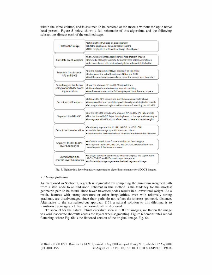
within the same volume, and is assumed to be centered at the macula without the optic nerve head present. Figure 5 below shows a full schematic of this algorithm, and the following subsections discuss each of the outlined steps.

Fig. 5. Eight retinal layer boundary segmentation algorithm schematic for SDOCT images.

3.1 Image flattening

As mentioned in Section 2, a graph is segmented by computing the minimum weighted path from a start node to an end node. Inherent in this method is the tendency for the shortest geometric path to be found, since fewer traversed nodes results in a lower total weight. As a result, features with strong curvature or other irregularities, even with relatively strong gradients, are disadvantaged since their paths do not reflect the shortest geometric distance. Alternative to the normalized-cut approach [17], a natural solution to this dilemma is to transform the image such that the desired path is shortened.

To account for the natural retinal curvature seen in SDOCT images, we flatten the image to avoid inaccurate shortcuts across the layers when segmenting. Figure 6 demonstrates retinal flattening, where Fig. 6b is the flattened version of the original image, Fig. 6a.


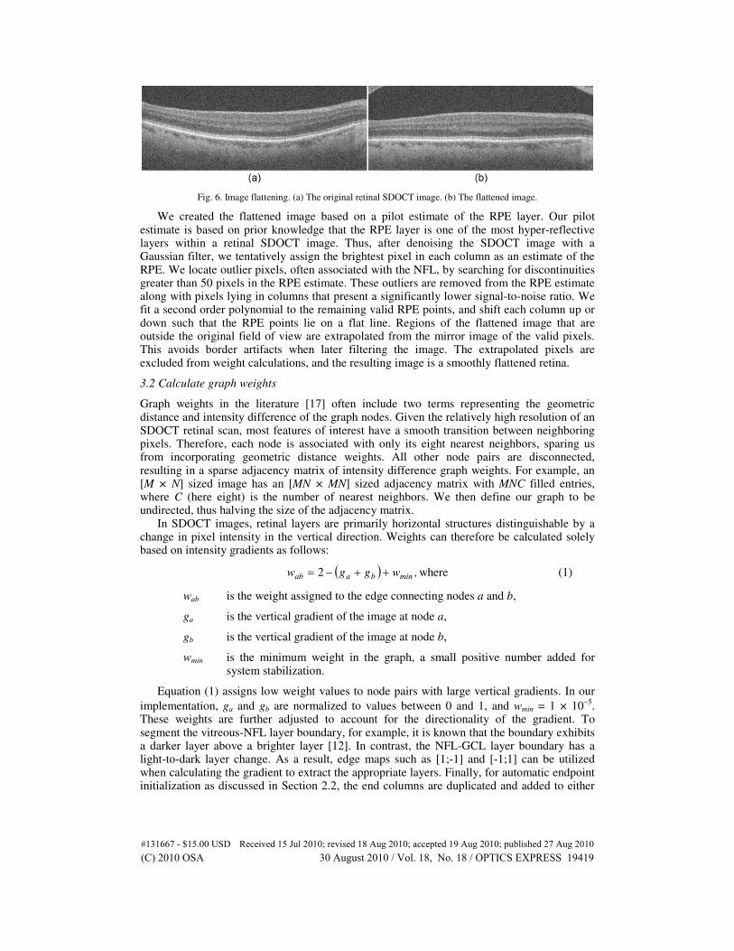
Fig. 6. Image flattening. (a) The original retinal SDOCT image. (b) The flattened image.

We created the flattened image based on a pilot estimate of the RPE layer. Our pilot estimate is based on prior knowledge that the RPE layer is one of the most hyper-reflective layers within a retinal SDOCT image. Thus, after denoising the SDOCT image with a Gaussian filter, we tentatively assign the brightest pixel in each column as an estimate of the RPE. We locate outlier pixels, often associated with the NFL, by searching for discontinuities greater than 50 pixels in the RPE estimate. These outliers are removed from the RPE estimate along with pixels lying in columns that present a significantly lower signal-to-noise ratio. We fit a second order polynomial to the remaining valid RPE points, and shift each column up or down such that the RPE points lie on a flat line. Regions of the flattened image that are outside the original field of view are extrapolated from the mirror image of the valid pixels. This avoids border artifacts when later filtering the image. The extrapolated pixels are excluded from weight calculations, and the resulting image is a smoothly flattened retina.

3.2 Calculate graph weights

Graph weights in the literature [17] often include two terms representing the geometric distance and intensity difference of the graph nodes. Given the relatively high resolution of an SDOCT retinal scan, most features of interest have a smooth transition between neighboring pixels. Therefore, each node is associated with only its eight nearest neighbors, sparing us from incorporating geometric distance weights. All other node pairs are disconnected, resulting in a sparse adjacency matrix of intensity difference graph weights. For example, an [M × N] sized image has an [MN × MN] sized adjacency matrix with MNC filled entries, where C (here eight) is the number of nearest neighbors. We then define our graph to be undirected, thus halving the size of the adjacency matrix.

In SDOCT images, retinal layers are primarily horizontal structures distinguishable by a change in pixel intensity in the vertical direction. Weights can therefore be calculated solely based on intensity gradients as follows:

( ) where2 ,wggw minbaab ++−= (1)

wab is the weight assigned to the edge connecting nodes a and b,

ga is the vertical gradient of the image at node a,

gb is the vertical gradient of the image at node b,

wmin is the minimum weight in the graph, a small positive number added for system stabilization.

Equation (1) assigns low weight values to node pairs with large vertical gradients. In our

implementation, ga and gb are normalized to values between 0 and 1, and wmin = 1 × 10−5

. These weights are further adjusted to account for the directionality of the gradient. To segment the vitreous-NFL layer boundary, for example, it is known that the boundary exhibits a darker layer above a brighter layer [12]. In contrast, the NFL-GCL layer boundary has a light-to-dark layer change. As a result, edge maps such as [1;-1] and [-1;1] can be utilized when calculating the gradient to extract the appropriate layers. Finally, for automatic endpoint initialization as discussed in Section 2.2, the end columns are duplicated and added to either


side of the image with vertical edge weights equal to wmin and all other weights following Eq. (1).

Our implementation for segmenting retinal layers in SDOCT images yields two undirected adjacency matrices sensitive to either dark-to-light or light-to-dark intensity transitions. For layer boundaries exhibiting a darker layer above a lighter layer such as the vitreous-NFL, INL-OPL, IS-OS, and OS-RPE boundaries, we utilize the dark-to-light adjacency matrix. In contrast, for the NFL-GCL, IPL-INL, OPL-PRNL, and RPE-choroid boundaries, which exhibit a lighter layer above a darker layer, we use the light-to-dark adjacency matrix.

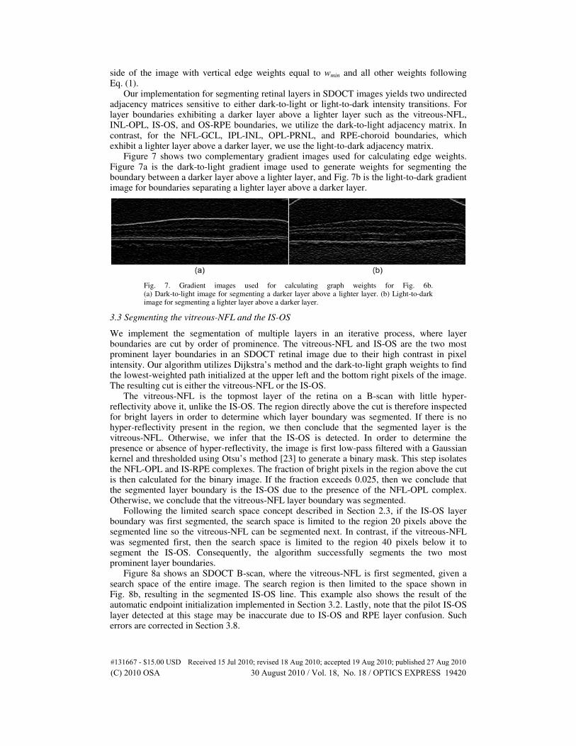
Figure 7 shows two complementary gradient images used for calculating edge weights. Figure 7a is the dark-to-light gradient image used to generate weights for segmenting the boundary between a darker layer above a lighter layer, and Fig. 7b is the light-to-dark gradient image for boundaries separating a lighter layer above a darker layer.

Fig. 7. Gradient images used for calculating graph weights for Fig. 6b. (a) Dark-to-light image for segmenting a darker layer above a lighter layer. (b) Light-to-dark image for segmenting a lighter layer above a darker layer.

3.3 Segmenting the vitreous-NFL and the IS-OS

We implement the segmentation of multiple layers in an iterative process, where layer boundaries are cut by order of prominence. The vitreous-NFL and IS-OS are the two most prominent layer boundaries in an SDOCT retinal image due to their high contrast in pixel intensity. Our algorithm utilizes Dijkstra’s method and the dark-to-light graph weights to find the lowest-weighted path initialized at the upper left and the bottom right pixels of the image. The resulting cut is either the vitreous-NFL or the IS-OS.

The vitreous-NFL is the topmost layer of the retina on a B-scan with little hyper-reflectivity above it, unlike the IS-OS. The region directly above the cut is therefore inspected for bright layers in order to determine which layer boundary was segmented. If there is no hyper-reflectivity present in the region, we then conclude that the segmented layer is the vitreous-NFL. Otherwise, we infer that the IS-OS is detected. In order to determine the presence or absence of hyper-reflectivity, the image is first low-pass filtered with a Gaussian kernel and thresholded using Otsu’s method [23] to generate a binary mask. This step isolates the NFL-OPL and IS-RPE complexes. The fraction of bright pixels in the region above the cut is then calculated for the binary image. If the fraction exceeds 0.025, then we conclude that the segmented layer boundary is the IS-OS due to the presence of the NFL-OPL complex. Otherwise, we conclude that the vitreous-NFL layer boundary was segmented.

Following the limited search space concept described in Section 2.3, if the IS-OS layer boundary was first segmented, the search space is limited to the region 20 pixels above the segmented line so the vitreous-NFL can be segmented next. In contrast, if the vitreous-NFL was segmented first, then the search space is limited to the region 40 pixels below it to segment the IS-OS. Consequently, the algorithm successfully segments the two most prominent layer boundaries.

Figure 8a shows an SDOCT B-scan, where the vitreous-NFL is first segmented, given a search space of the entire image. The search region is then limited to the space shown in Fig. 8b, resulting in the segmented IS-OS line. This example also shows the result of the automatic endpoint initialization implemented in Section 3.2. Lastly, note that the pilot IS-OS layer detected at this stage may be inaccurate due to IS-OS and RPE layer confusion. Such errors are corrected in Section 3.8.


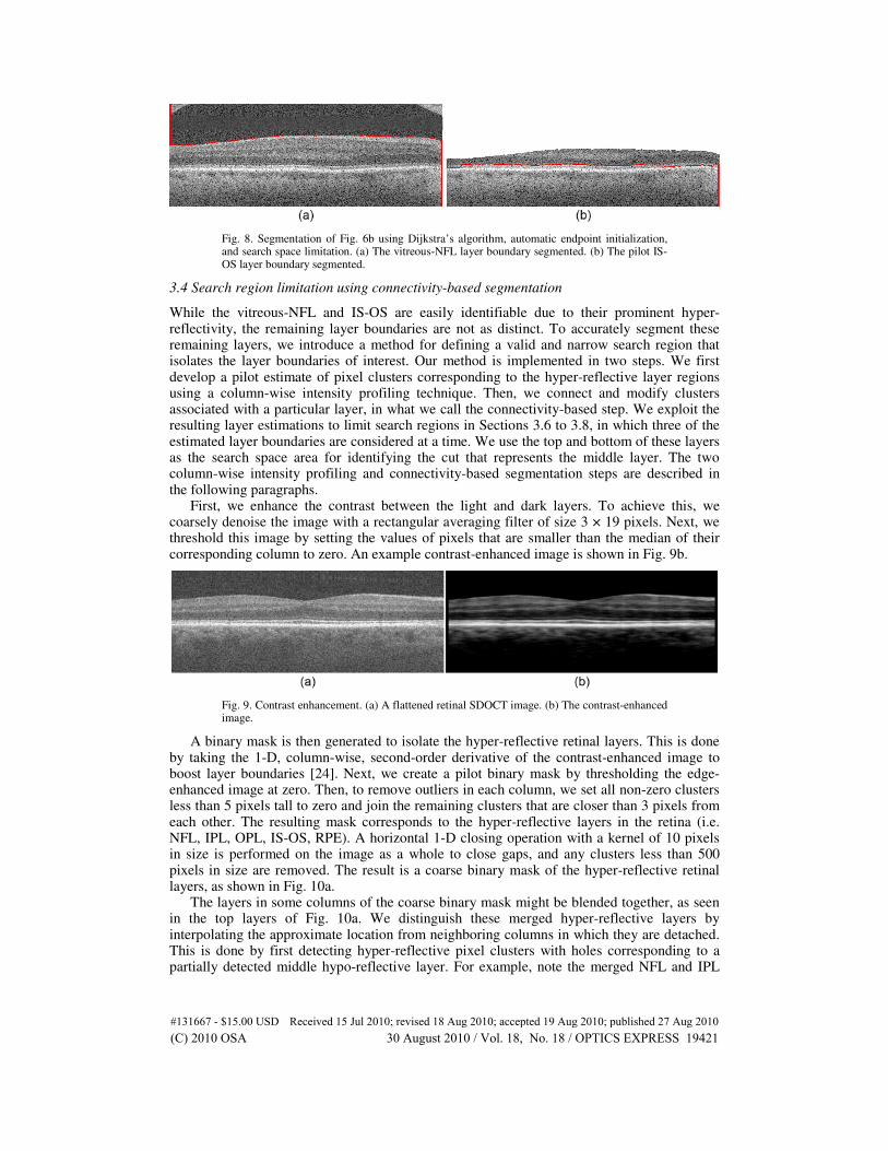
Fig. 8. Segmentation of Fig. 6b using Dijkstra’s algorithm, automatic endpoint initialization, and search space limitation. (a) The vitreous-NFL layer boundary segmented. (b) The pilot IS-OS layer boundary segmented.

3.4 Search region limitation using connectivity-based segmentation

While the vitreous-NFL and IS-OS are easily identifiable due to their prominent hyper-reflectivity, the remaining layer boundaries are not as distinct. To accurately segment these remaining layers, we introduce a method for defining a valid and narrow search region that isolates the layer boundaries of interest. Our method is implemented in two steps. We first develop a pilot estimate of pixel clusters corresponding to the hyper-reflective layer regions using a column-wise intensity profiling technique. Then, we connect and modify clusters associated with a particular layer, in what we call the connectivity-based step. We exploit the resulting layer estimations to limit search regions in Sections 3.6 to 3.8, in which three of the estimated layer boundaries are considered at a time. We use the top and bottom of these layers as the search space area for identifying the cut that represents the middle layer. The two column-wise intensity profiling and connectivity-based segmentation steps are described in the following paragraphs.

First, we enhance the contrast between the light and dark layers. To achieve this, we coarsely denoise the image with a rectangular averaging filter of size 3 × 19 pixels. Next, we threshold this image by setting the values of pixels that are smaller than the median of their corresponding column to zero. An example contrast-enhanced image is shown in Fig. 9b.

Fig. 9. Contrast enhancement. (a) A flattened retinal SDOCT image. (b) The contrast-enhanced image.

A binary mask is then generated to isolate the hyper-reflective retinal layers. This is done by taking the 1-D, column-wise, second-order derivative of the contrast-enhanced image to boost layer boundaries [24]. Next, we create a pilot binary mask by thresholding the edge-enhanced image at zero. Then, to remove outliers in each column, we set all non-zero clusters less than 5 pixels tall to zero and join the remaining clusters that are closer than 3 pixels from each other. The resulting mask corresponds to the hyper-reflective layers in the retina (i.e. NFL, IPL, OPL, IS-OS, RPE). A horizontal 1-D closing operation with a kernel of 10 pixels in size is performed on the image as a whole to close gaps, and any clusters less than 500 pixels in size are removed. The result is a coarse binary mask of the hyper-reflective retinal layers, as shown in Fig. 10a.

The layers in some columns of the coarse binary mask might be blended together, as seen in the top layers of Fig. 10a. We distinguish these merged hyper-reflective layers by interpolating the approximate location from neighboring columns in which they are detached. This is done by first detecting hyper-reflective pixel clusters with holes corresponding to a partially detected middle hypo-reflective layer. For example, note the merged NFL and IPL


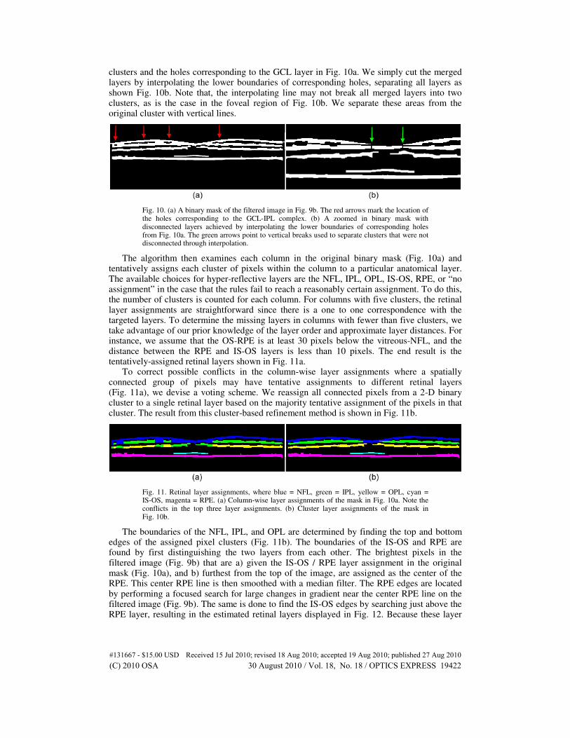
clusters and the holes corresponding to the GCL layer in Fig. 10a. We simply cut the merged layers by interpolating the lower boundaries of corresponding holes, separating all layers as shown Fig. 10b. Note that, the interpolating line may not break all merged layers into two clusters, as is the case in the foveal region of Fig. 10b. We separate these areas from the original cluster with vertical lines.

Fig. 10. (a) A binary mask of the filtered image in Fig. 9b. The red arrows mark the location of the holes corresponding to the GCL-IPL complex. (b) A zoomed in binary mask with disconnected layers achieved by interpolating the lower boundaries of corresponding holes from Fig. 10a. The green arrows point to vertical breaks used to separate clusters that were not disconnected through interpolation.

The algorithm then examines each column in the original binary mask (Fig. 10a) and tentatively assigns each cluster of pixels within the column to a particular anatomical layer. The available choices for hyper-reflective layers are the NFL, IPL, OPL, IS-OS, RPE, or “no assignment” in the case that the rules fail to reach a reasonably certain assignment. To do this, the number of clusters is counted for each column. For columns with five clusters, the retinal layer assignments are straightforward since there is a one to one correspondence with the targeted layers. To determine the missing layers in columns with fewer than five clusters, we take advantage of our prior knowledge of the layer order and approximate layer distances. For instance, we assume that the OS-RPE is at least 30 pixels below the vitreous-NFL, and the distance between the RPE and IS-OS layers is less than 10 pixels. The end result is the tentatively-assigned retinal layers shown in Fig. 11a.

To correct possible conflicts in the column-wise layer assignments where a spatially connected group of pixels may have tentative assignments to different retinal layers (Fig. 11a), we devise a voting scheme. We reassign all connected pixels from a 2-D binary cluster to a single retinal layer based on the majority tentative assignment of the pixels in that cluster. The result from this cluster-based refinement method is shown in Fig. 11b.

Fig. 11. Retinal layer assignments, where blue = NFL, green = IPL, yellow = OPL, cyan = IS-OS, magenta = RPE. (a) Column-wise layer assignments of the mask in Fig. 10a. Note the conflicts in the top three layer assignments. (b) Cluster layer assignments of the mask in Fig. 10b.

The boundaries of the NFL, IPL, and OPL are determined by finding the top and bottom edges of the assigned pixel clusters (Fig. 11b). The boundaries of the IS-OS and RPE are found by first distinguishing the two layers from each other. The brightest pixels in the filtered image (Fig. 9b) that are a) given the IS-OS / RPE layer assignment in the original mask (Fig. 10a), and b) furthest from the top of the image, are assigned as the center of the RPE. This center RPE line is then smoothed with a median filter. The RPE edges are located by performing a focused search for large changes in gradient near the center RPE line on the filtered image (Fig. 9b). The same is done to find the IS-OS edges by searching just above the RPE layer, resulting in the estimated retinal layers displayed in Fig. 12. Because these layer


estimations still contain errors, they are refined in the subsequent subsections using Dijkstra’s method, with adjacent layer estimations as search region boundaries.

Fig. 12. Connectivity-based segmentation of retinal layers using the layer assignments from Fig. 11b.

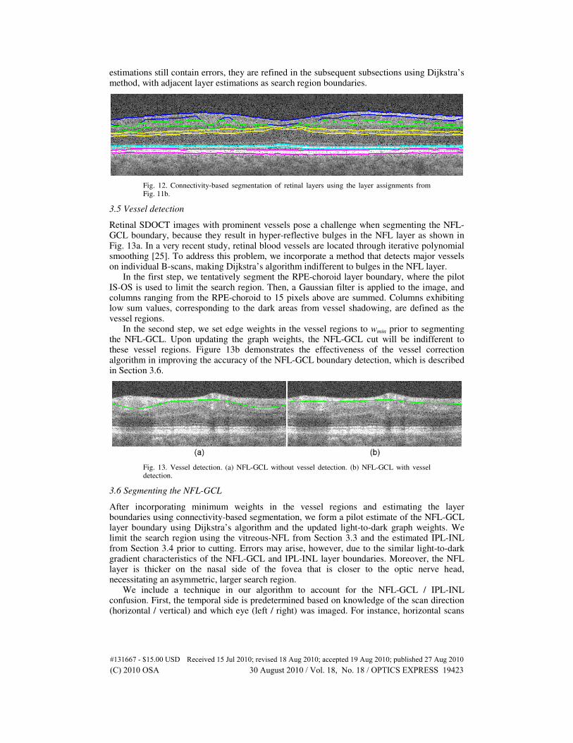
3.5 Vessel detection

Retinal SDOCT images with prominent vessels pose a challenge when segmenting the NFL-GCL boundary, because they result in hyper-reflective bulges in the NFL layer as shown in Fig. 13a. In a very recent study, retinal blood vessels are located through iterative polynomial smoothing [25]. To address this problem, we incorporate a method that detects major vessels on individual B-scans, making Dijkstra’s algorithm indifferent to bulges in the NFL layer.

In the first step, we tentatively segment the RPE-choroid layer boundary, where the pilot IS-OS is used to limit the search region. Then, a Gaussian filter is applied to the image, and columns ranging from the RPE-choroid to 15 pixels above are summed. Columns exhibiting low sum values, corresponding to the dark areas from vessel shadowing, are defined as the vessel regions.

In the second step, we set edge weights in the vessel regions to wmin prior to segmenting the NFL-GCL. Upon updating the graph weights, the NFL-GCL cut will be indifferent to these vessel regions. Figure 13b demonstrates the effectiveness of the vessel correction algorithm in improving the accuracy of the NFL-GCL boundary detection, which is described in Section 3.6.

Fig. 13. Vessel detection. (a) NFL-GCL without vessel detection. (b) NFL-GCL with vessel detection.

3.6 Segmenting the NFL-GCL

After incorporating minimum weights in the vessel regions and estimating the layer boundaries using connectivity-based segmentation, we form a pilot estimate of the NFL-GCL layer boundary using Dijkstra’s algorithm and the updated light-to-dark graph weights. We limit the search region using the vitreous-NFL from Section 3.3 and the estimated IPL-INL from Section 3.4 prior to cutting. Errors may arise, however, due to the similar light-to-dark gradient characteristics of the NFL-GCL and IPL-INL layer boundaries. Moreover, the NFL layer is thicker on the nasal side of the fovea that is closer to the optic nerve head, necessitating an asymmetric, larger search region.

We include a technique in our algorithm to account for the NFL-GCL / IPL-INL confusion. First, the temporal side is predetermined based on knowledge of the scan direction (horizontal / vertical) and which eye (left / right) was imaged. For instance, horizontal scans


of the left eye exhibit layer thinning on the right side of the fovea, whereas vertical scans of the left eye show layer thinning on both sides of the fovea.

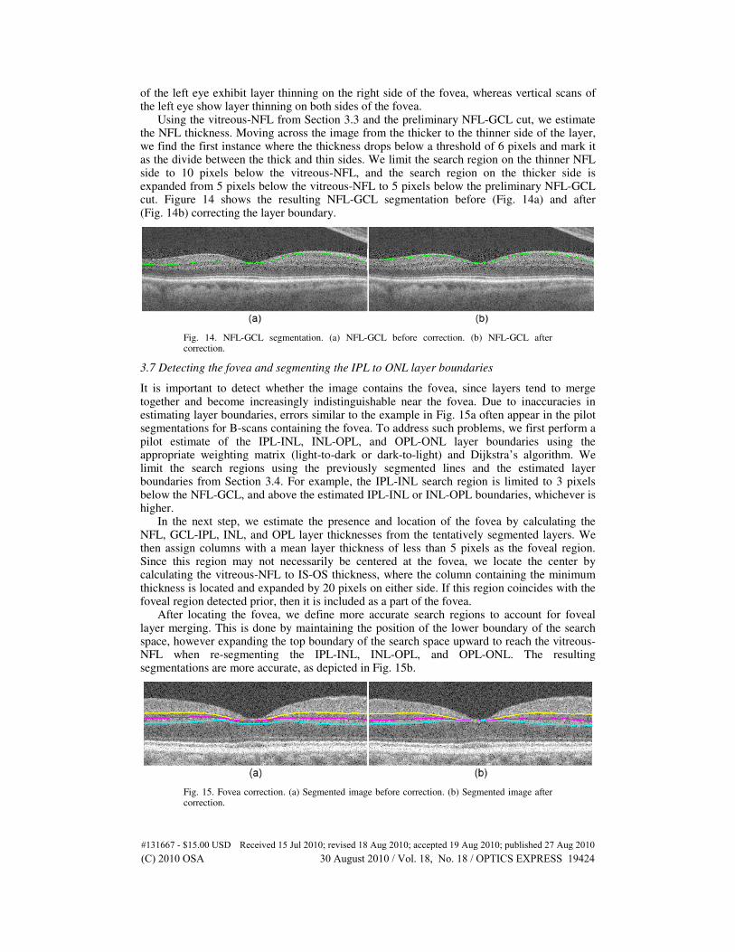
Using the vitreous-NFL from Section 3.3 and the preliminary NFL-GCL cut, we estimate the NFL thickness. Moving across the image from the thicker to the thinner side of the layer, we find the first instance where the thickness drops below a threshold of 6 pixels and mark it as the divide between the thick and thin sides. We limit the search region on the thinner NFL side to 10 pixels below the vitreous-NFL, and the search region on the thicker side is expanded from 5 pixels below the vitreous-NFL to 5 pixels below the preliminary NFL-GCL cut. Figure 14 shows the resulting NFL-GCL segmentation before (Fig. 14a) and after (Fig. 14b) correcting the layer boundary.

Fig. 14. NFL-GCL segmentation. (a) NFL-GCL before correction. (b) NFL-GCL after correction.

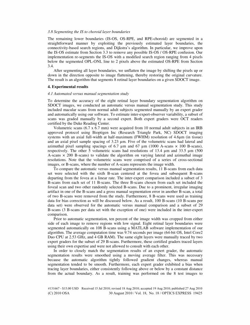
3.7 Detecting the fovea and segmenting the IPL to ONL layer boundaries

It is important to detect whether the image contains the fovea, since layers tend to merge together and become increasingly indistinguishable near the fovea. Due to inaccuracies in estimating layer boundaries, errors similar to the example in Fig. 15a often appear in the pilot segmentations for B-scans containing the fovea. To address such problems, we first perform a pilot estimate of the IPL-INL, INL-OPL, and OPL-ONL layer boundaries using the appropriate weighting matrix (light-to-dark or dark-to-light) and Dijkstra’s algorithm. We limit the search regions using the previously segmented lines and the estimated layer boundaries from Section 3.4. For example, the IPL-INL search region is limited to 3 pixels below the NFL-GCL, and above the estimated IPL-INL or INL-OPL boundaries, whichever is higher.

In the next step, we estimate the presence and location of the fovea by calculating the NFL, GCL-IPL, INL, and OPL layer thicknesses from the tentatively segmented layers. We then assign columns with a mean layer thickness of less than 5 pixels as the foveal region. Since this region may not necessarily be centered at the fovea, we locate the center by calculating the vitreous-NFL to IS-OS thickness, where the column containing the minimum thickness is located and expanded by 20 pixels on either side. If this region coincides with the foveal region detected prior, then it is included as a part of the fovea.

After locating the fovea, we define more accurate search regions to account for foveal layer merging. This is done by maintaining the position of the lower boundary of the search space, however expanding the top boundary of the search space upward to reach the vitreous-NFL when re-segmenting the IPL-INL, INL-OPL, and OPL-ONL. The resulting segmentations are more accurate, as depicted in Fig. 15b.

Fig. 15. Fovea correction. (a) Segmented image before correction. (b) Segmented image after correction.


3.8 Segmenting the IS to choroid layer boundaries

The remaining lower boundaries (IS-OS, OS-RPE, and RPE-choroid) are segmented in a straightforward manner by exploiting the previously estimated layer boundaries, the connectivity-based search regions, and Dijkstra’s algorithm. In particular, we improve upon the IS-OS estimate from Section 3.3 to remove any possible IS-OS / OS-RPE confusion. Our implementation re-segments the IS-OS with a modified search region ranging from 4 pixels below the segmented OPL-ONL line to 2 pixels above the estimated OS-RPE from Section 3.4.

After segmenting all layer boundaries, we unflatten the image by shifting the pixels up or down in the direction opposite to image flattening, thereby restoring the original curvature. The result is an algorithm that segments 8 retinal layer boundaries on a given SDOCT image.

4. Experimental results

4.1 Automated versus manual segmentation study

To determine the accuracy of the eight retinal layer boundary segmentation algorithm on SDOCT images, we conducted an automatic versus manual segmentation study. This study included macular scans from normal adult subjects segmented manually by an expert grader and automatically using our software. To estimate inter-expert-observer variability, a subset of scans was graded manually by a second expert. Both expert graders were OCT readers certified by the Duke Reading Center.

Volumetric scans (6.7 x 6.7 mm) were acquired from 10 normal adult subjects in an IRB approved protocol using Bioptigen Inc (Research Triangle Park, NC) SDOCT imaging systems with an axial full-width at half-maximum (FWHM) resolution of 4.6µm (in tissue) and an axial pixel sample spacing of 3.23 µm. Five of the volumetric scans had lateral and azimuthal pixel sampling spacings of 6.7 µm and 67 µm (1000 A-scans × 100 B-scans), respectively. The other 5 volumetric scans had resolutions of 13.4 µm and 33.5 µm (500 A-scans × 200 B-scans) to validate the algorithm on varying lateral and azimuthal image resolutions. Note that the volumetric scans were comprised of a series of cross-sectional images, or B-scans, where the number of A-scans represents the image width.

To compare the automatic versus manual segmentation results, 11 B-scans from each data set were selected with the sixth B-scan centered at the fovea and subsequent B-scans departing from the fovea at a linear rate. The inter-expert comparison included a subset of 3 B-scans from each set of 11 B-scans. The three B-scans chosen from each set included the foveal scan and two other randomly selected B-scans. Due to a prominent, irregular imaging artifact in one of the B-scans and a gross manual segmentation error in another B-scan, a total of two B-scans were removed from the study. Furthermore, 8 B-scans were used as training data for bias correction as will be discussed below. As a result, 100 B-scans (10 B-scans per data set) were observed for the automatic versus manual comparison and a subset of 29 B-scans (3 B-scans per data set with the exception of one) were included in the inter-expert comparison.

Prior to automatic segmentation, ten percent of the image width was cropped from either side of each image to remove regions with low signal. Eight retinal layer boundaries were segmented automatically on 108 B-scans using a MATLAB software implementation of our algorithm. The average computation time was 9.74 seconds per image (64-bit OS, Intel Core2 Duo CPU at 2.53 GHz, and 4 GB RAM). The same eight layers were manually traced by two expert graders for the subset of 29 B-scans. Furthermore, these certified graders traced layers using their own expertise and were not allowed to consult with each other.

In order to closely match the segmentation results of an expert grader, the automatic segmentation results were smoothed using a moving average filter. This was necessary because the automatic algorithm tightly followed gradient changes, whereas manual segmentation tended to be smooth. Furthermore, each expert grader exhibited a bias when tracing layer boundaries, either consistently following above or below by a constant distance from the actual boundary. As a result, training was performed on the 8 test images to


determine any segmentation biases from the manual grading. Each automatically segmented

layer in the set of 100 B-scans was then shifted up or down by bias values of −0.9, −0.8, −1.0,

−1.3, −1.6, −1.3, −0.3, and −0.6 pixels, respectively, in order to mimic the segmentation behavior of the manual grader.

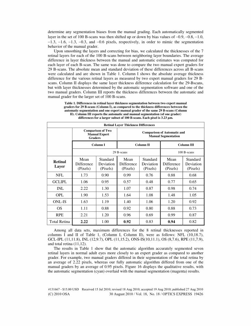
Upon smoothing the layers and correcting for bias, we calculated the thicknesses of the 7 retinal layers for each of the 100 B-scans between neighboring layer boundaries. The average difference in layer thickness between the manual and automatic estimates was computed for each layer of each B-scan. The same was done to compare the two manual expert graders for 29 B-scans. The absolute mean and standard deviation of these differences across all B-scans were calculated and are shown in Table 1. Column I shows the absolute average thickness difference for the various retinal layers as measured by two expert manual graders for 29 B-scans. Column II displays the same layer thickness difference calculation for the 29-Bscans, but with layer thicknesses determined by the automatic segmentation software and one of the two manual graders. Column III reports the thickness differences between the automatic and manual grader for the larger set of 100 B-scans.

Table 1. Differences in retinal layer thickness segmentation between two expert manual graders for 29 B-scans (Column I), as compared to the thickness differences between the automatic segmentation and one expert manual grader of the same 29 B-scans (Column

II). Column III reports the automatic and manual segmentation (of one grader) differences for a larger subset of 100 B-scans. Each pixel is 3.23 µm.

Retinal Layer Thickness Differences

Comparison of Two

Manual Expert Graders

Comparison of Automatic and Manual Segmentation

Column I Column II Column III

29 B-scans 100 B-scans

Retinal Layer

Mean Difference

(Pixels)

Standard Deviation (Pixels)

Mean Difference

(Pixels)


Mean Difference

(Pixels)


NFL 1.73 0.90 0.99 0.76 0.88 0.68

GCLIPL 1.06 0.95 0.57 0.48 0.77 0.65

INL 2.22 1.30 1.07 0.87 0.98 0.74

OPL 1.90 1.53 1.64 1.08 1.48 1.05

ONL-IS 1.63 1.19 1.40 1.06 1.20 0.92

OS 1.11 0.88 0.92 0.80 0.88 0.73

RPE 2.21 1.20 0.96 0.69 0.99 0.87

Total Retina 2.22 1.00 0.92 0.83 0.94 0.82

Among all data sets, maximum differences for the 8 retinal thicknesses reported in columns I and II of Table 1, (Column I, Column II), were as follows: NFL (10,18.7), GCL-IPL (11,11.8), INL (12,9.7), OPL (11,15.2), ONS-IS(10,11.1), OS (8,7.6), RPE (11,7.9), and total retina (11,12).

The results in Table 1 show that the automatic algorithm accurately segmented seven retinal layers in normal adult eyes more closely to an expert grader as compared to another grader. For example, two manual graders differed in their segmentation of the total retina by an average of 2.22 pixels, whereas our fully automatic algorithm differed from one of the manual graders by an average of 0.95 pixels. Figure 16 displays the qualitative results, with the automatic segmentation (cyan) overlaid with the manual segmentation (magenta) results.


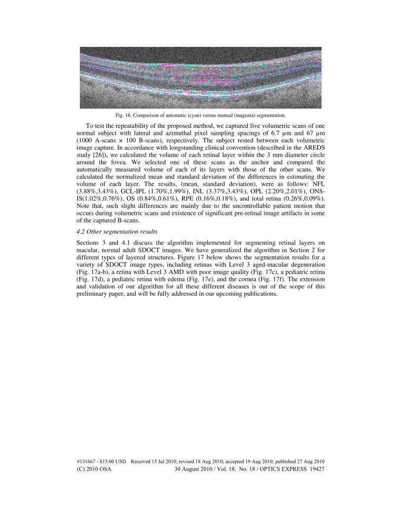
Fig. 16. Comparison of automatic (cyan) versus manual (magenta) segmentation.

To test the repeatability of the proposed method, we captured five volumetric scans of one normal subject with lateral and azimuthal pixel sampling spacings of 6.7 µm and 67 µm (1000 A-scans × 100 B-scans), respectively. The subject rested between each volumetric image capture. In accordance with longstanding clinical convention (described in the AREDS study [26]), we calculated the volume of each retinal layer within the 3 mm diameter circle around the fovea. We selected one of these scans as the anchor and compared the automatically measured volume of each of its layers with those of the other scans. We calculated the normalized mean and standard deviation of the differences in estimating the volume of each layer. The results, (mean, standard deviation), were as follows: NFL (3.88%,3.43%), GCL-IPL (1.70%,1.99%), INL (3.37%,3.43%), OPL (2.20%,2.01%), ONS-IS(1.02%,0.76%), OS (0.84%,0.61%), RPE (0.16%,0.18%), and total retina (0.26%,0.09%). Note that, such slight differences are mainly due to the uncontrollable patient motion that occurs during volumetric scans and existence of significant pre-retinal image artifacts in some of the captured B-scans.

4.2 Other segmentation results

Sections 3 and 4.1 discuss the algorithm implemented for segmenting retinal layers on macular, normal adult SDOCT images. We have generalized the algorithm in Section 2 for different types of layered structures. Figure 17 below shows the segmentation results for a variety of SDOCT image types, including retinas with Level 3 aged-macular degeneration (Fig. 17a-b), a retina with Level 3 AMD with poor image quality (Fig. 17c), a pediatric retina (Fig. 17d), a pediatric retina with edema (Fig. 17e), and the cornea (Fig. 17f). The extension and validation of our algorithm for all these different diseases is out of the scope of this preliminary paper, and will be fully addressed in our upcoming publications.


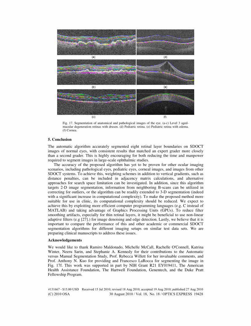
Fig. 17. Segmentation of anatomical and pathological images of the eye. (a-c) Level 3 aged-macular degeneration retinas with drusen. (d) Pediatric retina. (e) Pediatric retina with edema. (f) Cornea.

5. Conclusion

The automatic algorithm accurately segmented eight retinal layer boundaries on SDOCT images of normal eyes, with consistent results that matched an expert grader more closely than a second grader. This is highly encouraging for both reducing the time and manpower required to segment images in large-scale ophthalmic studies.

The accuracy of the proposed algorithm has yet to be proven for other ocular imaging scenarios, including pathological eyes, pediatric eyes, corneal images, and images from other SDOCT systems. To achieve this, weighting schemes in addition to vertical gradients, such as distance penalties, can be included in adjacency matrix calculations, and alternative approaches for search space limitation can be investigated. In addition, since this algorithm targets 2-D image segmentation, information from neighboring B-scans can be utilized in correcting for outliers, or the algorithm can be readily extended to 3-D segmentation (indeed with a significant increase in computational complexity). To make the proposed method more suitable for use in clinic, its computational complexity should be reduced. We expect to achieve this by exploiting more efficient computer programming languages (e.g. C instead of MATLAB) and taking advantage of Graphics Processing Units (GPUs). To reduce filter smoothing artifacts, especially for thin retinal layers, it might be beneficial to use non-linear adaptive filters (e.g [27].) for image denoising and edge detection. Lastly, we believe that it is important to compare the performance of this and other academic or commercial SDOCT segmentation algorithms for different imaging setups on similar test data sets. We are preparing clinical manuscripts to address these issues.

Acknowledgements

We would like to thank Ramiro Maldonado, Michelle McCall, Rachelle O'Connell, Katrina Winter, Neeru Sarin, and Stephanie A. Kennedy for their contributions to the Automatic versus Manual Segmentation Study, Prof. Rebecca Willett for her invaluable comments, and Prof. Anthony N. Kuo for providing and Francesco LaRocca for segmenting the image in Fig. 17f. This work was supported in part by NIH Grant R21 EY019411, The American Health Assistance Foundation, The Hartwell Foundation, Genentech, and the Duke Pratt Fellowship Program.


Documents

Automatic segmentation of seven retinal layers in SDOCT images congruent with expert manual segmentation