Availability analysis of banking server with warm · PDF fileAssociate Professor M.M. (P.G.) College, Fatehabad-125050 (Haryana), India Introduction

~ 24 ~

International Journal of Statistics and Applied Mathematics 2016; 1(2): 24-35

ISSN: 2456-1452

Maths 2016; 1(2): 24-35

© 2016 Stats & Maths

www.mathsjournal.com

Received: 08-05-2016

Accepted: 09-06-2016

Raj Kumar

Research Scholar, J.J.T.

University, Jhunjhnu

(Rajasthan), India

Dr. Pardeep Goel

Associate Professor M.M. (P.G.)

College, Fatehabad-125050

(Haryana), India

Correspondence:

Raj Kumar

Research Scholar, J.J.T.

University, Jhunjhnu

(Rajasthan), India

Availability analysis of banking server with warm

standby

Raj Kumar and Dr. Pardeep Goel

Abstract

Availability analysis of a local banking server with a remote standby server is analyzed for system

parameters using Regenerative Point Graphical Technique (RPGT).

Keywords: Availability, Regenerative Point Graphical Technique (RPGT), System Parameters, Local

Server, Remote Server

Introduction

In banking industry all the data relating to transaction history along with authorization is

stored in local sever (Bank branch) and stand-by remote server. As data in baking industry is

very important for customers and the management, daily data and transaction history of a

branch are stored in the branch and also by the manager of the branch in the hard disc at the

time of closing daily/regularly. Considering the importance of individual units in system

Kumar, J. & Malik, S. C. [1] have discussed the concept of preventive maintenance for a single

unit system. Liu., R. [2], Malik, S. C. [3], Nakagawa, T. and Osaki, S. [4] have discussed

reliability analysis of a one unit system with un-repairable spare units and its applications.

Goel, P. & Singh J. [5], Gupta, P., Singh, J. & Singh, I.P. [6], Kumar, S. & Goel, P. [7], Gupta, V.

K. [8], Chaudhary, Goel & Kumar [9] Sharma & Goel [10], Ritikesh & Goel [11] and Goyal &

Goel [12] have discussed behavior with perfect and imperfect switch-over of systems using

various techniques. All the transaction history is stored in the remote server simultaneously

because in case of failure of local server data may be retrieved from the remote server.

The failure rate of local server is much higher than that of the remote server which may be due

to poor local environmental conditions such as electricity failure, earth quake, inefficient data

operator and other local conditions. Remote server has better maintenance and environmental

conditions as the data of all branches stored in the remote server. The management maintains

better environment conditions of remote server, hence the failure rates of local server are

higher than that of remote server and repair rates of local server is poor than that of remote

server. On failure of local server data is retrieved from the remote server for the smooth

functioning of the banking industry i.e. remote server works as warm stand to local server.

Taking constant failure rates & repair rates with remote server as standby to local server a

transition diagram of the system is drawn.

The system consists of local server ‘A’ and standby remote server ‘B’. There may be times

when some of the banking operations may not be carried out by A or B, then the system works

in reduced capacity. If the failure rate of local server ‘A’ to reduced state is λ1, and from

reduced state to failed state is λ2 and repair rate of local server from reduced state to A is w2

and from failed state to reduce state is w1 similarly for the remote server B with failure rates

λ3, λ4 and repair rates w4 and w3. It is assumed that when any of servers fails then the system is

not put to use.

Fuzzy concept is used to determine failure/working state of a unit. Taking failure rates

exponential, repair rates general & independent and taking into consideration various

probabilities, a transition diagram of the system is developed to find Primary circuits,

~ 25 ~

International Journal of Statistics and Applied Mathematics Secondary circuits & Tertiary circuits and Base state. Problem is solved using RPGT to determine system parameters. System

behavior is discussed with the help of graphs and tables. Particular cases for arm, cold and hot standby cases are taken to study the

effect of failure and repair rates on system parameters. Tables and Graphs are drawn to compare the results.

Assumptions and Notations

The following assumptions and notations are taken: -

1. A single repair facility is available.

2. The distributions of failure times and repair times are exponential and general respectively and also different.

3. Failures and repairs are statistically independent.

4. Repair is perfect and repaired system is as good as new one.

5. Nothing can fail when the system is in failed state.

6. The system is discussed for steady-state conditions.

7. Replacement of Un-repairable unit and repair facility is immediate.

8. There are separate repairmen for local and remote servers.

: A circuit formed through un-failed states.

m-cycle: A circuit (may be formed through regenerative or non-regenerative / failed state) whose terminals are at the regenerative

state m.

: A circuit (may be formed through un-failed regenerative or non-regenerative state) whose terminals are at the

regenerative m state.

: r-th directed simple path from i-state to j-state; r takes positive integral values

for different paths from i-state to j-state.

: A directed simple failure free path from -state to i-state.

Vm,m : Probability factor of the state m reachable from the terminal state m of the

m-cycle.

: Probability factor of the state m reachable from the terminal state m of the

.

Ri (t): Reliability of the system at time t, given that the system entered the un-failed

Regenerative state ‘i’ at t = 0.

Ai (t) : Probability of the system in up time at time ‘t’, given that the system entered

Regenerative state ‘i’ at t = 0.

Bi (t) : Reliability that the server is busy for doing a particulars job at time ‘t’; given

That the system entered regenerative state ‘i’ at t = 0.

Vi (t) : The expected no. of server visits for doing a job in (o,t] given that the system

Entered regenerative state ‘i’ at t = 0.

‘,’ denote derivative

Wi (t) : Probability that the server is busy doing a particular job at time t without transiting to any other regenerative state ‘i’

through one or more non-regenerative states, given that the system entered the regenerative state ‘i’ at t = 0.

μi : Mean sojourn time spent in state i, before visiting any other states;

=

: The total un-conditional time spent before transiting to any other regenerative states, given that the system entered

regenerative state ‘i’ at t=0.

Ni : Expected waiting time spent while doing a given job, given that the system entered regenerative state ‘i’ at t=0;

ξ : Base state of the system.

fj : Fuzziness measure of the j-state.

λ1 : Constant failure rate of server A from full working state to reduce state.

λ2 : Constant failure rate of local server from reduce state to complete failure.

λ3 : Constant failure rate of remote server from full working to failed state.

λ4 : constant failure rate of remote server from reduced state to complete failed

state.

Regenerative State

Reduced State

Failed State

A/ /a : Unit in full capacity working / reduced state / failed state.

Similarly for the remote server B.

~ 26 ~

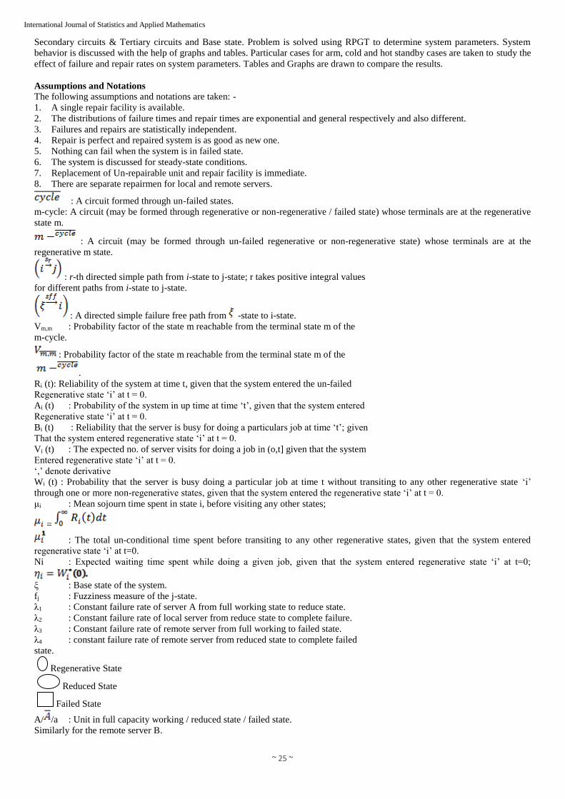
International Journal of Statistics and Applied Mathematics Taking into consideration the above assumptions and notations the Transition Diagram of the system is given in Figure 1.

S0 = AB, S1 = B, S2 = A ,

S3 = aB, S4 = Ab

Fig 1: The possible transitions rates between states along with transition states

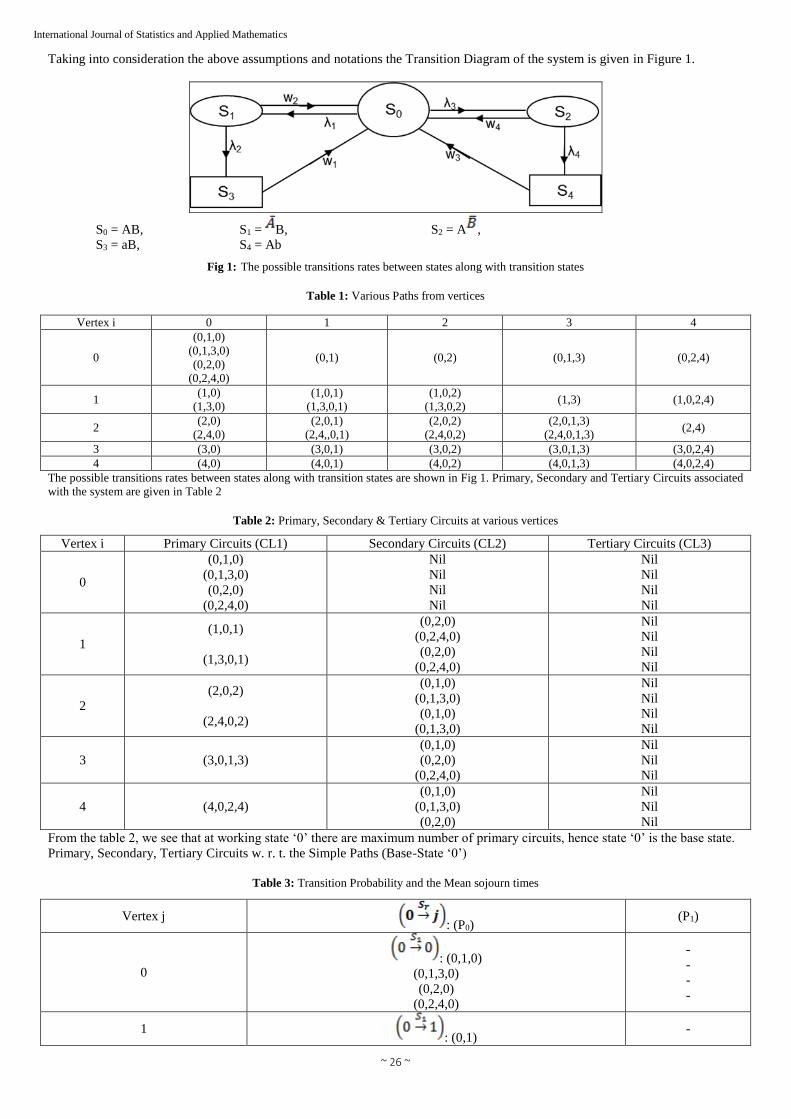
Table 1: Various Paths from vertices

Vertex i 0 1 2 3 4

0

(0,1,0)

(0,1,3,0)

(0,2,0)

(0,2,4,0)

(0,1) (0,2) (0,1,3) (0,2,4)

1 (1,0)

(1,3,0)

(1,0,1)

(1,3,0,1)

(1,0,2)

(1,3,0,2) (1,3) (1,0,2,4)

2 (2,0)

(2,4,0)

(2,0,1)

(2,4,,0,1)

(2,0,2)

(2,4,0,2)

(2,0,1,3)

(2,4,0,1,3) (2,4)

3 (3,0) (3,0,1) (3,0,2) (3,0,1,3) (3,0,2,4)

4 (4,0) (4,0,1) (4,0,2) (4,0,1,3) (4,0,2,4)

The possible transitions rates between states along with transition states are shown in Fig 1. Primary, Secondary and Tertiary Circuits associated

with the system are given in Table 2

Table 2: Primary, Secondary & Tertiary Circuits at various vertices

Vertex i Primary Circuits (CL1) Secondary Circuits (CL2) Tertiary Circuits (CL3)

0

(0,1,0)

(0,1,3,0)

(0,2,0)

(0,2,4,0)

Nil

Nil

Nil

Nil

Nil

Nil

Nil

Nil

1

(1,0,1)

(1,3,0,1)

(0,2,0)

(0,2,4,0)

(0,2,0)

(0,2,4,0)

Nil

Nil

Nil

Nil

2

(2,0,2)

(2,4,0,2)

(0,1,0)

(0,1,3,0)

(0,1,0)

(0,1,3,0)

Nil

Nil

Nil

Nil

3 (3,0,1,3)

(0,1,0)

(0,2,0)

(0,2,4,0)

Nil

Nil

Nil

4 (4,0,2,4)

(0,1,0)

(0,1,3,0)

(0,2,0)

Nil

Nil

Nil

From the table 2, we see that at working state ‘0’ there are maximum number of primary circuits, hence state ‘0’ is the base state.

Primary, Secondary, Tertiary Circuits w. r. t. the Simple Paths (Base-State ‘0’)

Table 3: Transition Probability and the Mean sojourn times

Vertex j : (P0)

(P1)

0 : (0,1,0)

(0,1,3,0)

(0,2,0)

(0,2,4,0)

-

-

-

-

1 : (0,1)

-

~ 27 ~

International Journal of Statistics and Applied Mathematics

2 : (0,2)

-

3 : (0,1,3)

-

4 : (0,2,4)

-

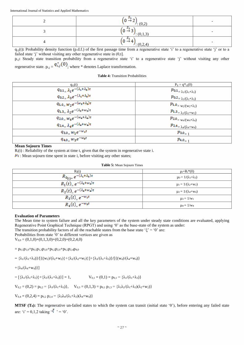
qi,j(t): Probability density function (p.d.f.) of the first passage time from a regenerative state ‘i’ to a regenerative state ‘j’ or to a

failed state ‘j’ without visiting any other regenerative state in (0,t].

pi,j: Steady state transition probability from a regenerative state ‘i’ to a regenerative state ‘j’ without visiting any other

regenerative state. pi,j = ; where * denotes Laplace transformation.

Table 4: Transition Probabilities

qi,j(t) Pij = q*i,j(0)

=

=

= λ1/(λ1+λ3)

= λ3/(λ1+λ3)

=

=

= w2/(w2+λ2)

= λ2/(λ2+w2)

=

=

= w4/(w4+λ4)

= λ4/(λ4+w4)

= = 1

= = 1

Mean Sojourn Times

Ri(t) : Reliability of the system at time t, given that the system in regenerative state i.

: Mean sojourn time spent in state i, before visiting any other states;

Table 5: Mean Sojourn Times

Ri(t) µi=Ri*(0)

(t)= µ0 = 1/(λ1+λ3)

= µ1 = 1/(λ2+w2)

= µ2 = 1/(λ4+w4)

= µ3 = 1/w1

= µ4 = 1/w4

Evaluation of Parameters

The Mean time to system failure and all the key parameters of the system under steady state conditions are evaluated, applying

Regenerative Point Graphical Technique (RPGT) and using ‘0’ as the base-state of the system as under:

The transition probability factors of all the reachable states from the base state ‘ξ’ = ‘0’ are:

Probabilities from state ‘0’ to different vertices are given as

V0,0 = (0,1,0)+(0,1,3,0)+(0,2,0)+(0,2,4,0)

= p0,1p1,0+p0,1p1,3p3,0+p0,2p2,0+p0,2p2,4p4,0

= {λ1/(λ1+λ3)}/[{(w2)/(λ2+w2)}+{λ2/(λ2+w2)}]+{λ3/(λ1+λ3)}/[{(w4)/(λ4+w4)}

+{λ4/(λ4+w4)}]

= [{λ1/(λ1+λ3)}+{λ3/(λ1+λ3)}] = 1, V0,1 = (0,1) = p0,1 = {λ1/(λ1+λ3)}

V0,2 = (0,2) = p0,2 = {λ3/(λ1+λ3)}, V0,3 = (0,1,3) = p0,1 p1,3 = {λ1λ2/(λ1+λ3)(λ2+w2)}

V0,4 = (0,2,4) = p0,2 p2,4 = {λ3λ4/(λ1+λ3)(λ4+w4)}

MTSF (T0): The regenerative un-failed states to which the system can transit (initial state ‘0’), before entering any failed state

are: ‘i’ = 0,1,2 taking ‘ ’ = ‘0’.

~ 28 ~


MTSF (T0) = ÷

T0 = (V0,0μ0+V0,1μ1+V0,2μ2)/{1-(0,1,0)-(0,2,0)}

= (V0,0μ0+V0,1μ1+V0,2μ2)/(1- p0,1p1,0- p0,2p2,0)

= (K1+K2+K3)/(1-p0,1p1,0- p0,2p2,0), where K1 = V0,0μ0, K2 = V0,1μ1, K3 = V0,2μ2

Availability of the System (A0): The regenerative states at which the system is available are ‘j’ = 0, 1, 2 and the regenerative

states are ‘i’ = 0,1,2,3,4 taking ‘ξ’ = ‘0’ the total fraction of time for which the system is available is given by

A0= ÷

A0 =

A0 = (V0,0f0µ0+V0,1f1µ1+V0,2f2µ2)/(V0,0µ01+V0,1µ1

1+V0,2µ21+V0,3µ3

1+V0,4µ41)

As fj = 1, for j = 0,1,2 and fj = 0 for j = 3,4 Taking

Let K = (V0,0µ0+V0,1µ1+V0,2µ2+V0,3µ3+V0,4µ4) = K1+K2+K3+K4+K5

= (V0,0µ0+V0,1µ1+V0,2µ2)/K, = (K1+K2+K3)/K

Busy Period of the Server: The regenerative states are 1 ≤ j ≤ 4 where server is busy while doing repairs and regenerative states

are ‘i’ = 0 to 4 taking ξ = ‘0’, the total fraction of time for which the server remains busy is

B0= ÷

B0 =

B0 = (V0,1η1+V0,2η2+V0,3η3+V0,4η4)/(V0,0 µ0+V0,1µ1 +V0,2µ2+V0,3µ3+V0,4 µ4)

Taking

= {1-(V0,0μ0)/K}, = (1-μ0/K), = (1-K1/K)

Expected Number of Inspections by the repair man: The regenerative states where the repair man do this job j = 1,2 the

regenerative states are i = 0 to 4, Taking ‘ξ’ = ‘0’, the number of visit by the repair man is given by

V0= ÷

V0 =

V0 = (V0,1+V0,2)/(V0,0µ0+V0,1µ1+V0,2µ2+V0,3µ3+V0,4µ4)

= (V0,1+V0,2)/K, = [{λ1/(λ1+λ3)}+{λ3/(λ1+λ3)}]/K, = 1/K

Particular Cases

Warm Stand -by Case

K = K1+K2+K3+K4+K5 K1 = V0,0μ0 = {1/(λ1+λ3)}

K2 = V0,1μ1 = {λ1/(λ1+λ3)(λ2+w2)}, K3 = V0,2μ2 = {λ3/(λ1+λ3)(λ4+w4)}

K4 = V0,3μ3 = {λ1λ2/(λ1+λ3)(λ2+w2)w1}, K5 = V0,4μ4 = {λ3λ4/(λ1+λ3)(λ4+w4)}

p0,1 p1,0 = {λ1w2/(λ1+λ3)(λ2+w2)}, p0,2 p2,0 = {λ3w4/(λ1+λ3)(λ4+w4)}

λ3 = λ4 = 0.001

~ 29 ~

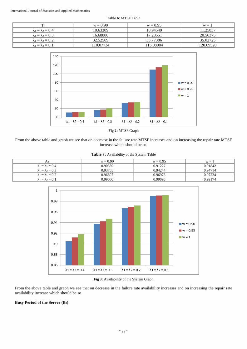
International Journal of Statistics and Applied Mathematics Table 6: MTSF Table

T0 w = 0.90 w = 0.95 w = 1

λ1 = λ2 = 0.4 10.63309 10.94549 11.25837

λ1 = λ2 = 0.3 16.68000 17.23551 20.56375

λ1 = λ2 = 0.2 32.52569 33.77386 35.02725

λ1 = λ2 = 0.1 110.07734 115.08004 120.09520

Fig 2: MTSF Graph

From the above table and graph we see that on decrease in the failure rate MTSF increases and on increasing the repair rate MTSF

increase which should be so.

Table 7: Availability of the System Table

A0 w = 0.90 w = 0.95 w = 1

λ1 = λ2 = 0.4 0.90539 0.91227 0.91842

λ1 = λ2 = 0.3 0.93755 0.94244 0.94714

λ1 = λ2 = 0.2 0.96697 0.96978 0.97224

λ1 = λ2 = 0.1 0.99000 0.99093 0.99174

Fig 3: Availability of the System Graph

From the above table and graph we see that on decrease in the failure rate availability increases and on increasing the repair rate

availability increase which should be so.

Busy Period of the Server (B0)

~ 30 ~

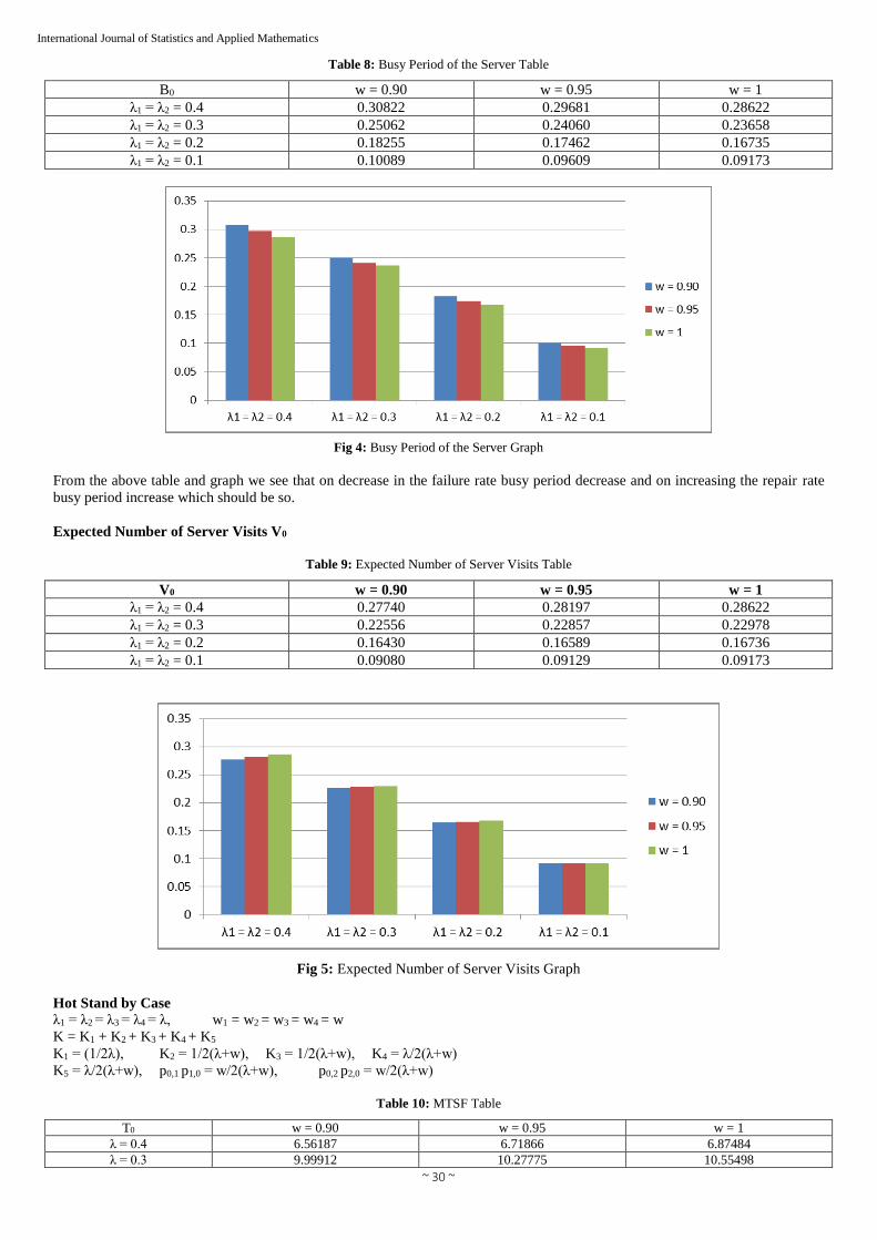
International Journal of Statistics and Applied Mathematics Table 8: Busy Period of the Server Table

B0 w = 0.90 w = 0.95 w = 1

λ1 = λ2 = 0.4 0.30822 0.29681 0.28622

λ1 = λ2 = 0.3 0.25062 0.24060 0.23658

λ1 = λ2 = 0.2 0.18255 0.17462 0.16735

λ1 = λ2 = 0.1 0.10089 0.09609 0.09173

Fig 4: Busy Period of the Server Graph

From the above table and graph we see that on decrease in the failure rate busy period decrease and on increasing the repair rate

busy period increase which should be so.

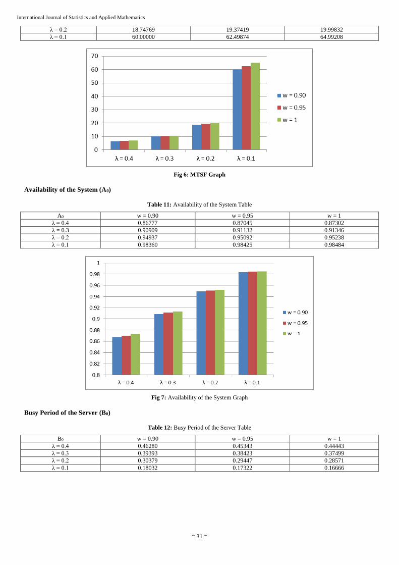
Expected Number of Server Visits V0

Table 9: Expected Number of Server Visits Table

V0 w = 0.90 w = 0.95 w = 1

λ1 = λ2 = 0.4 0.27740 0.28197 0.28622

λ1 = λ2 = 0.3 0.22556 0.22857 0.22978

λ1 = λ2 = 0.2 0.16430 0.16589 0.16736

λ1 = λ2 = 0.1 0.09080 0.09129 0.09173

Fig 5: Expected Number of Server Visits Graph

Hot Stand by Case

λ1 = λ2 = λ3 = λ4 = λ, w1 = w2 = w3 = w4 = w

K = K1 + K2 + K3 + K4 + K5

K1 = (1/2λ), K2 = 1/2(λ+w), K3 = 1/2(λ+w), K4 = λ/2(λ+w)

K5 = λ/2(λ+w), p0,1 p1,0 = w/2(λ+w), p0,2 p2,0 = w/2(λ+w)

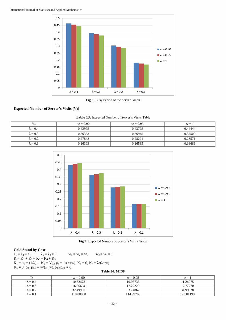
Table 10: MTSF Table

T0 w = 0.90 w = 0.95 w = 1

λ = 0.4 6.56187 6.71866 6.87484

λ = 0.3 9.99912 10.27775 10.55498

~ 31 ~

International Journal of Statistics and Applied Mathematics λ = 0.2 18.74769 19.37419 19.99832

λ = 0.1 60.00000 62.49874 64.99208

Fig 6: MTSF Graph

Availability of the System (A0)

Table 11: Availability of the System Table

A0 w = 0.90 w = 0.95 w = 1

λ = 0.4 0.86777 0.87045 0.87302

λ = 0.3 0.90909 0.91132 0.91346

λ = 0.2 0.94937 0.95092 0.95238

λ = 0.1 0.98360 0.98425 0.98484



Table 12: Busy Period of the Server Table

B0 w = 0.90 w = 0.95 w = 1

λ = 0.4 0.46280 0.45343 0.44443

λ = 0.3 0.39393 0.38423 0.37499

λ = 0.2 0.30379 0.29447 0.28571

λ = 0.1 0.18032 0.17322 0.16666

~ 32 ~



Expected Number of Server’s Visits (V0)

Table 13: Expected Number of Server’s Visits Table

V0 w = 0.90 w = 0.95 w = 1

λ = 0.4 0.42975 0.43725 0.44444

λ = 0.3 0.36363 0.36945 0.37500

λ = 0.2 0.27848 0.28221 0.28571

λ = 0.1 0.16393 0.16535 0.16666

Fig 9: Expected Number of Server’s Visits Graph

Cold Stand by Case

λ1 = λ2 = λ, λ3 = λ4 = 0, w1 = w2 = w, w3 = w4 = 1

K = K1 + K2 + K3 + K4 + K5

K1 = μ0 = (1/λ), K2 = V0,1 μ1 = 1/(λ+w), K3 = 0, K4 = λ/(λ+w)

K5 = 0, p0,1 p1,0 = w/(λ+w), p0,2 p2,0 = 0 Table 14: MTSF

T0 w = 0.90 w = 0.95 w = 1

λ = 0.4 10.62473 10.93736 11.24975

λ = 0.3 16.66664 17.22220 17.77770

λ = 0.2 32.49967 33.74862 34.99928

λ = 0.1 110.00000 114.99769 120.01199

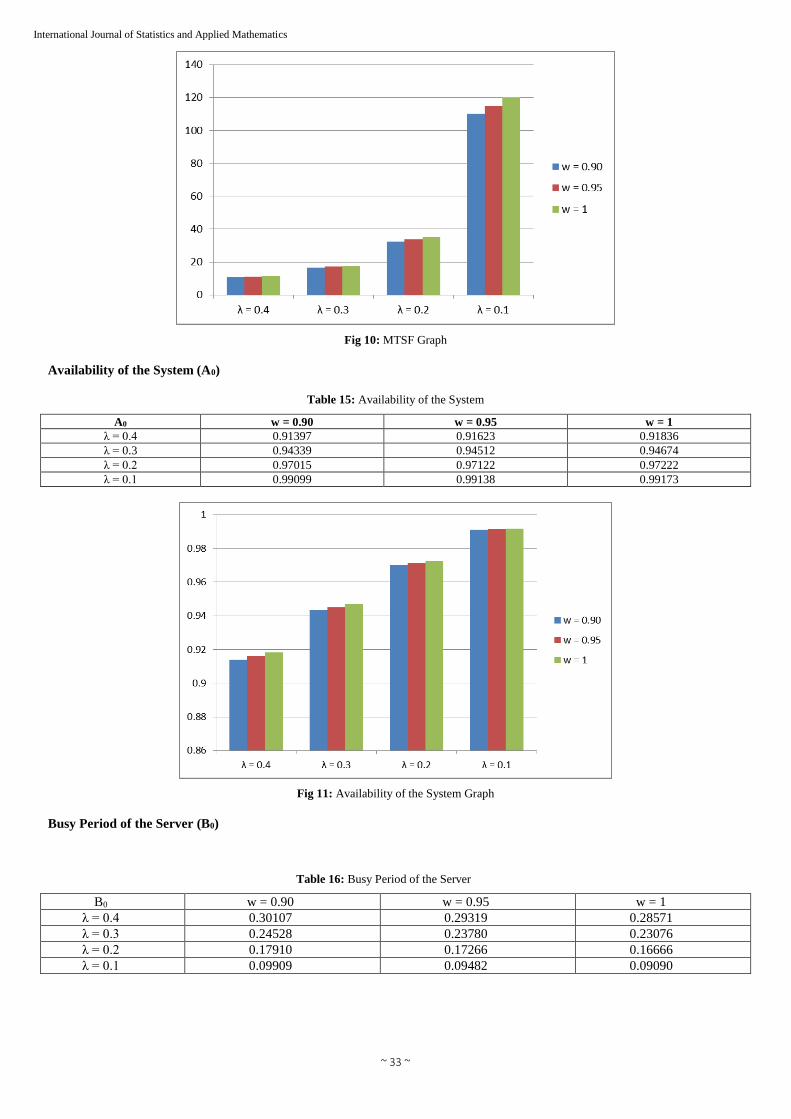
~ 33 ~


Fig 10: MTSF Graph

Availability of the System (A0)

Table 15: Availability of the System

A0 w = 0.90 w = 0.95 w = 1

λ = 0.4 0.91397 0.91623 0.91836

λ = 0.3 0.94339 0.94512 0.94674

λ = 0.2 0.97015 0.97122 0.97222

λ = 0.1 0.99099 0.99138 0.99173



Table 16: Busy Period of the Server

B0 w = 0.90 w = 0.95 w = 1

λ = 0.4 0.30107 0.29319 0.28571

λ = 0.3 0.24528 0.23780 0.23076

λ = 0.2 0.17910 0.17266 0.16666

λ = 0.1 0.09909 0.09482 0.09090

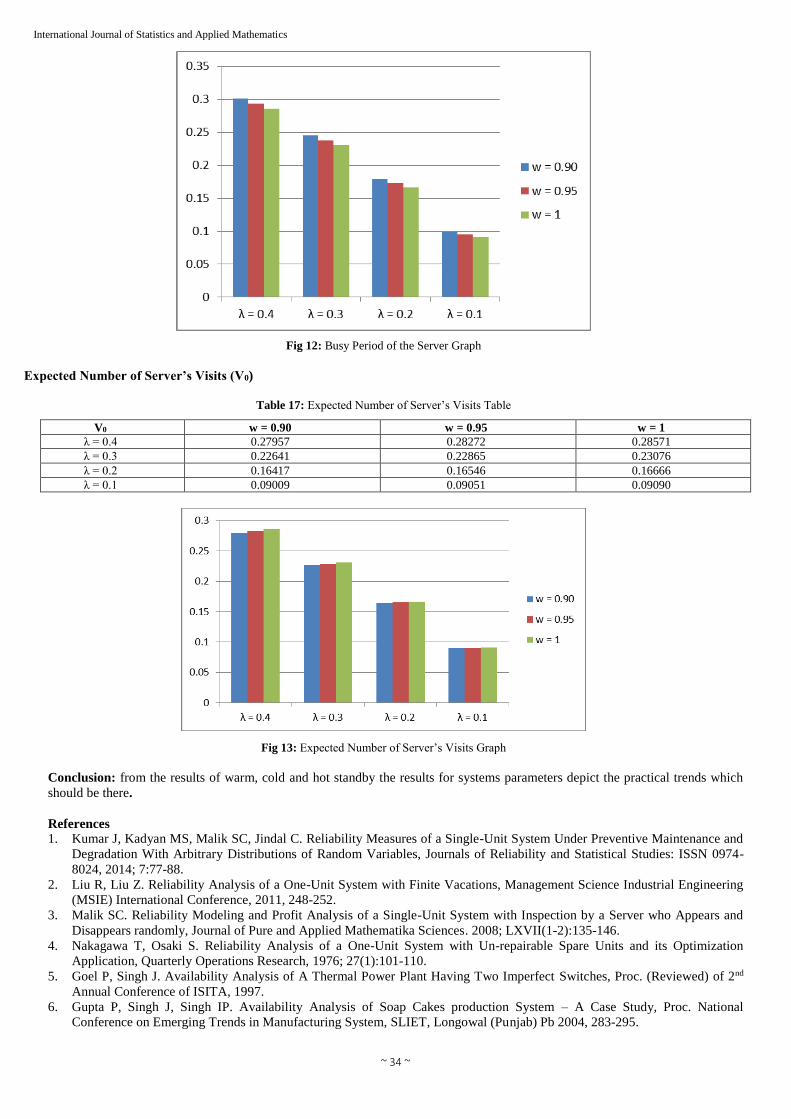
~ 34 ~



Expected Number of Server’s Visits (V0)

Table 17: Expected Number of Server’s Visits Table

V0 w = 0.90 w = 0.95 w = 1

λ = 0.4 0.27957 0.28272 0.28571

λ = 0.3 0.22641 0.22865 0.23076

λ = 0.2 0.16417 0.16546 0.16666

λ = 0.1 0.09009 0.09051 0.09090

Fig 13: Expected Number of Server’s Visits Graph

Conclusion: from the results of warm, cold and hot standby the results for systems parameters depict the practical trends which

should be there.

References

1. Kumar J, Kadyan MS, Malik SC, Jindal C. Reliability Measures of a Single-Unit System Under Preventive Maintenance and

Degradation With Arbitrary Distributions of Random Variables, Journals of Reliability and Statistical Studies: ISSN 0974-

8024, 2014; 7:77-88.

2. Liu R, Liu Z. Reliability Analysis of a One-Unit System with Finite Vacations, Management Science Industrial Engineering

(MSIE) International Conference, 2011, 248-252.

3. Malik SC. Reliability Modeling and Profit Analysis of a Single-Unit System with Inspection by a Server who Appears and

Disappears randomly, Journal of Pure and Applied Mathematika Sciences. 2008; LXVII(1-2):135-146.

4. Nakagawa T, Osaki S. Reliability Analysis of a One-Unit System with Un-repairable Spare Units and its Optimization

Application, Quarterly Operations Research, 1976; 27(1):101-110.

5. Goel P, Singh J. Availability Analysis of A Thermal Power Plant Having Two Imperfect Switches, Proc. (Reviewed) of 2nd

Annual Conference of ISITA, 1997.

6. Gupta P, Singh J, Singh IP. Availability Analysis of Soap Cakes production System – A Case Study, Proc. National

Conference on Emerging Trends in Manufacturing System, SLIET, Longowal (Punjab) Pb 2004, 283-295.

~ 35 ~

International Journal of Statistics and Applied Mathematics 7. Kumar S, Goel P. Availability Analysis of Two Different Units System with a Standby Having Imperfect Switch Over Device

in Banking Industry, Aryabhatta Journal of Mathematics & Informatics. ISSN: 0975-7139, 2014; 6(2):299-304.

8. Gupta V K. Analysis of a single unit system using a base state: Aryabhatta J of Maths & Info. 2011; 3(1):59-66.

9. Chaudhary Nidhi, Goel P, Kumar Surender. Developing the reliability model for availability and behavior analysis of a

distillery using Regenerative Point Graphical Technique.: ISSN (Online): 2347-1697, 2013; 1(iv):26-40.

10. Sharma Sandeep P. Behavioral Analysis of Whole Grain Flour Mill Using RPGT. ISBN 978-93-325-4896-1, ICETESMA-15,

2015, 194-201.

11. Ritikesh Goel. Availability Modeling of Single Unit System Subject to Degradation Post Repair after Complete Failure Using

RPGT. ISSN 2347-8527, September, 2015.

12. Goyal Goel. Behavioral Analysis of Two Unit System with Preventive Maintenance and Degradation in One Unit after

Complete Failure Using RPGT. ISSN 2347-8527. 2015; 4:190-197.

Documents

Availability analysis of banking server with warm · PDF fileAssociate Professor M.M. (P.G.) College, Fatehabad-125050 (Haryana), India Introduction