Average modeling and evaluation of 18-pulse

Turk J Elec Eng & Comp Sci(2018) 26: 3115 – 3129© TÜBİTAKdoi:10.3906/elk-1611-35

Turkish Journal of Electrical Engineering & Computer Sciences

http :// journa l s . tub i tak .gov . t r/e lektr ik/

Research Article

Average modeling and evaluation of 18-pulse autotransformer rectifier unitwithout interphase transformers

Shahbaz KHAN1,∗ , Xiaobin ZHANG1 , Husan ALI1 , Haider ZAMAN1 , Muhammad SAAD1 ,Bakht Muhammad KHAN2

1Department of Automation and Electrical Engineering, Faculty of Electronics Engineering,Northwestern Polytechnical University, Xian, P.R. China

2Department of Electronics and Information, Faculty of Electronics Engineering,Northwestern Polytechnical University, Xian, P.R. China

Received: 04.11.2016 • Accepted/Published Online: 17.09.2018 • Final Version: 29.11.2018

Abstract: This paper presents an improved average model and evaluation of an 18-pulse autotransformer rectifier unit(ATRU) in differential delta configuration. Average models remove the switching behavior of diode rectifiers and highbandwidth transients, which not only facilitates simulation of power systems by reducing computational cost but alsoenables impedance-based stability analysis for large complex power systems. To experimentally validate the proposedaverage model, a 2-kW, 18-pulse ATRU has been tested and the results of the derived model are compared with thoseof the switching model and experimental prototype. Computed transfer function of load impedance from the proposedaverage model closely resembles those of the switching model and the experimentally measured results validate themodeling procedure. Furthermore, stability analysis of the 18-pulse ATRU may be executed based on the return ratioof source and load impedance.

Key words: Autotransformer rectifier unit, return ratio, average models, high bandwidth transients

1. IntroductionThe last two decades have seen the aircraft industry focusing a lot of research on the concept of more electricaircraft. The systems utilizing nonelectrical energy in the aircraft have been partially or fully substituted withtheir electrical counterparts, which has led to the significant reduction of fossil fuel consumption [1]. Withthe rapidly growing applications of electrical power systems, in order to ensure higher efficiency and reliability,attempts are being made to minimize the size and weight of these systems.

The power conditioning, for ensuring a desired level of power quality, is achieved with the use of powerelectronic converters. The quality factors of the modern power converters are lower input current total harmonicdistortion (THD) and load voltage ripples [2]. The converter should also be characterized by high efficiency,small size, and long lifetime. Converter systems with either a voltage or current DC link are commonly used inindustrial applications [3]. With the developments of industries, harmonic distortion is increasing in industrialpower systems due to the constant growth of nonlinear loads such as rectifiers, inverters, or cycloconverters.These devices are likely to introduce significant harmonic pollution into the power systems, which may result inequipment malfunction and premature equipment failure, communication interference, or even the malfunctionof protective devices [4]. The concept of multiphase AC-DC converters, for reducing the input current THD,∗Correspondence: [email protected]

This work is licensed under a Creative Commons Attribution 4.0 International License.3115

https://orcid.org/0000-0002-0898-0491

https://orcid.org/0000-0002-9589-5825

https://orcid.org/0000-0002-9602-9259

https://orcid.org/0000-0001-6439-1133

https://orcid.org/0000-0002-7437-0675

https://orcid.org/0000-0003-4834-3443

KHAN et al./Turk J Elec Eng & Comp Sci

has been mentioned in the literature [5,6]. Input current harmonics generated in multipulse converters haveorders of 6kx ±1 with amplitudes of 1/6kx ±1, where k is any positive integer and x is the number of 3-phase rectifiers connected in parallel or series [7]. Six-pulse converters are the most common converters buttheir harmonic performance is poor and many aerospace power quality specifications now demand 12-pulseperformance or better. The use of a passive filter connected to the input of the six-pulse rectifier gives anunsatisfactory performance because of the variable frequency operation of the supply; therefore, higher pulserectifiers are the only viable solution to this problem [8]. Due to high performance, in aircraft electrical powersystems, the uncontrolled rectifier is a part of ATRUs that are widely used as front end converters for creationof DC distribution buses to drive motors such as fuel pumping, cabin pressurization and air conditioning, enginestart, and flight control actuation [9–11].

Conventionally, voltage transformers have been used for increasing the number of phases to introducethe appropriate phase shift for harmonic cancellation, but this technique is not preferred for more than12-pulse converters. Higher pulse converters require more than one conventional transformer, leading tohigher cost, larger volume, and weight of the overall system. ATRUs are employed in multipulse converters,comprising autotransformers for conversion of three-phase supply into n -phase systems using a 3-to-n -phaseautotransformer [12]. Within complex interconnected systems, one must have complete knowledge of thedynamic interactions among the subsystems so that one is in a position to be able to predict the stabilityof the overall system. The stability of every subsystem is computed from the Nyquist plot of its return ratio,the ratio of its source output impedance ZS to its load input impedance ZL [13]. Major difficulty lies in theproper extraction of these impedances for time-varying sources and loads. For DC systems, one can easilyextract these impedances through system linearization around a stable operating point, but in case of ACsystems, there is no stable operating point and hence different methods are to be applied in order to obtainstable operation point for system linearization such as dq0 transformation [14].

Stability analysis based on switching models results in increased computational complexity as well aslarge computer storage requirements. This leads to longer simulation times, especially when the overall systemcontains many switching models [15–17]. Dynamic average-value models (AVMs) have been utilized effectivelyto remove the high-frequency switching from the model while preserving the lower frequency dynamics ofthe system and provide accurate system-level steady-state and transient simulation results, which make suchmodels particularly suitable for large-scale studies of power electronic systems [18,19]. Average models convertsimulation models from discontinuous to continuous, which runs magnitudes faster than the original switchingmodels. This allows computationally efficient analysis of relatively slower dynamics, such as those involved inthe destabilizing phenomena that may arise due to the interaction between tightly regulated loads and energystorage components. Since AVMs are time-invariant, they can be numerically linearized about any operatingpoint for small-signal analysis, such as obtaining input/output impedances.

Two main techniques have been developed so far in order to derive average models of line commutatedconverters, namely the transfer function method [2] and mathematically derived models [20]. In the first method,the relation between input-output terminal parameters (voltage/current) is obtained for the respective switchingmodels. The data are curve-fitted to predict the operation of the model at different operating points. Thismodeling technique, also known as the parametric AVM approach, is easier and straightforward but requiresextensive simulations and the model is applicable to variable frequency systems. On the other hand, the secondmethod involves explicit mathematical calculations that offer improved results in terms of static and dynamicbehavior. In [21, 22], partial dynamic improvement in a model was achieved by considering linearly varying

3116


load current. However, the effect of linear load variation was ignored in computation of commutation angleand input current equations. The commutation angle depends only on the average load current during thecommutation period, not conduction.

This paper proposes the development of an explicit mathematical dynamic AVM of 18-pulse transformer-fed diode rectifiers, which is an improved model of the static model discussed in [23]. While deriving thedynamic model, addition of a linear term to the DC load current makes it match the detailed/switch modelmore precisely in steady as well as transient states. Static models are good in representing detailed modelsduring steady states but perform poorly during transient states since they do not account for load variation. Inthis proposed model, load current is assumed linearly varying throughout the averaging period (commutationand conduction) and is approximated using first-order Taylor series expansion that eases capturing the dynamiccharacteristics of the system more closely. This model is nonswitching and is in the dq0 frame; hence, it can beutilized to extract small-signal input and output impedances. Output impedance of the derived AVM is obtainedthrough linearization in MATLAB/Simulink, which is presented for comparison with output impedance of thehardware setup. It is evident from comparison that the derived AVM output impedance closely resembles thatof the hardware setup; hence, this model can be utilized for stability measurements of switch model ATRUs.

2. ATRU configuration

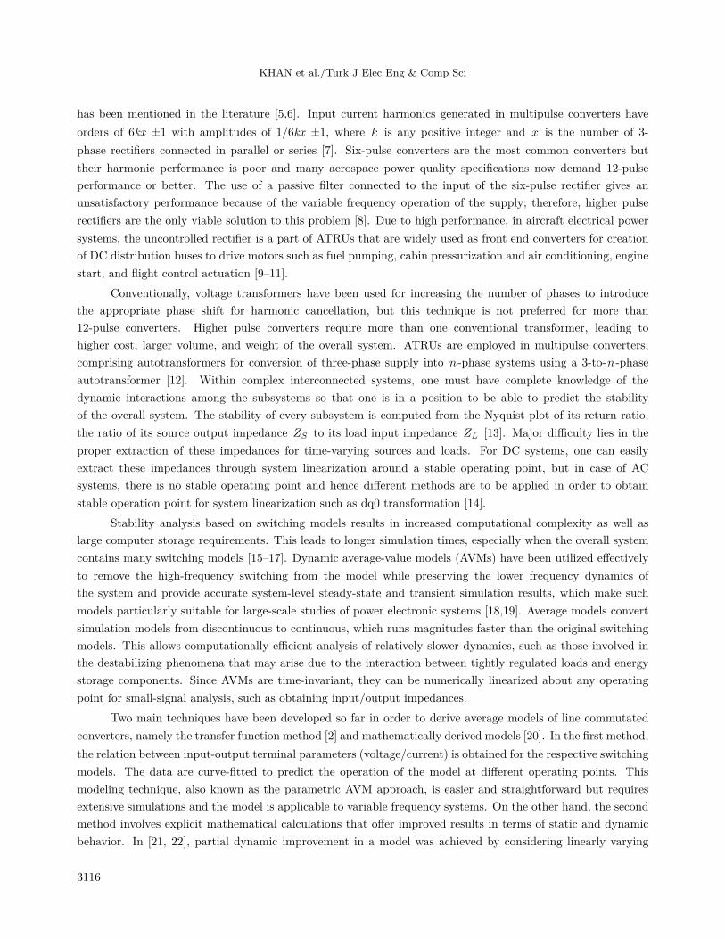
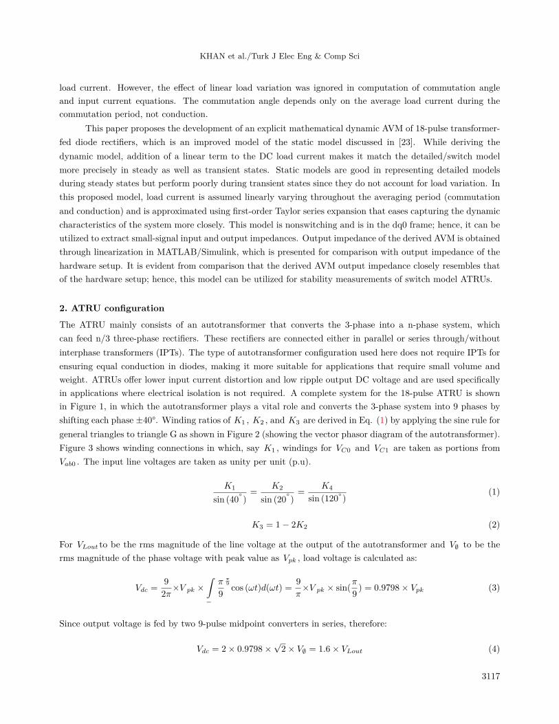
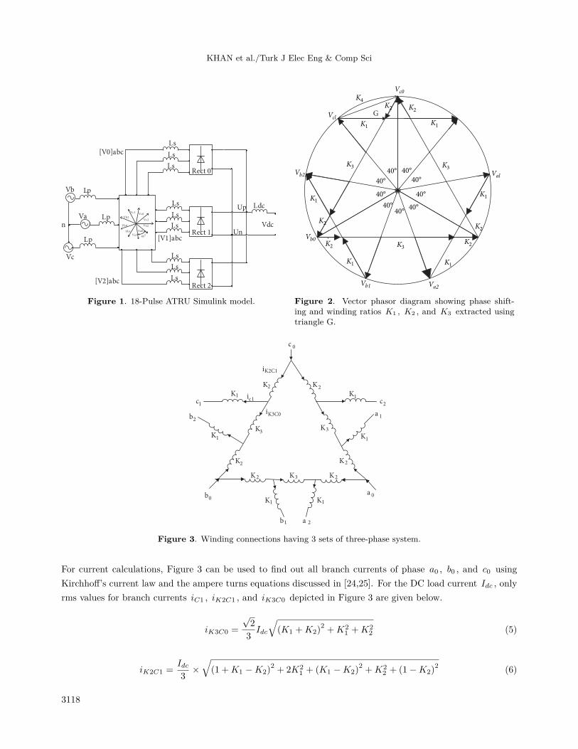
The ATRU mainly consists of an autotransformer that converts the 3-phase into a n-phase system, whichcan feed n/3 three-phase rectifiers. These rectifiers are connected either in parallel or series through/withoutinterphase transformers (IPTs). The type of autotransformer configuration used here does not require IPTs forensuring equal conduction in diodes, making it more suitable for applications that require small volume andweight. ATRUs offer lower input current distortion and low ripple output DC voltage and are used specificallyin applications where electrical isolation is not required. A complete system for the 18-pulse ATRU is shownin Figure 1, in which the autotransformer plays a vital role and converts the 3-phase system into 9 phases byshifting each phase ±40°. Winding ratios of K1 , K2 , and K3 are derived in Eq. (1) by applying the sine rule forgeneral triangles to triangle G as shown in Figure 2 (showing the vector phasor diagram of the autotransformer).Figure 3 shows winding connections in which, say K1 , windings for VC0 and VC1 are taken as portions fromVab0 . The input line voltages are taken as unity per unit (p.u).

K1

sin (40)=

K2

sin (20)=

K4

sin (120)

(1)

K3 = 1− 2K2 (2)

For VLout to be the rms magnitude of the line voltage at the output of the autotransformer and V∅ to be therms magnitude of the phase voltage with peak value as Vpk , load voltage is calculated as:

Vdc =9

2π×V pk ×

∫−

π

9

π9 cos (ωt)d(ωt) = 9

π×V pk × sin(π

9) = 0.9798× Vpk (3)

Since output voltage is fed by two 9-pulse midpoint converters in series, therefore:

Vdc = 2× 0.9798×√2× V∅ = 1.6× VLout (4)

3117


400Va1

Vb1

Vc 1

Vb2

Vb0

Vc2

Vc0

Va2

Va0

Ls[V0]abc

[V1]abc

[V2]abc

Vdc

Lp

Ldc

Va

Vb

Vc

n

Up

Rect 0

Rect 1

Rect 2

Ls

Ls

Ls

Ls

Ls

Ls

Ls

Ls

Lp

LpUn

G

40° 40°K3

K4

K1

K2

K2K2

Val

Vc0

Vcl

Vb2

Vb0

Vb1 Va2

K2

K2

K2

K1K1

K1 K1

K3

K3

K1

40°

40°

40°40°

40°

40°

40°

Figure 1. 18-Pulse ATRU Simulink model. Figure 2. Vector phasor diagram showing phase shift-ing and winding ratios K1 , K2 , and K3 extracted usingtriangle G.

0c

1c

2c

0a

1a

2a

0b

1b

2b

1K

1K

1K

1K

1K

1K

2K

2K 2K

2K

2K2

K

3K

3K 3K

1ci

i

K3C0

K2C1

i

Figure 3. Winding connections having 3 sets of three-phase system.

For current calculations, Figure 3 can be used to find out all branch currents of phase a0 , b0 , and c0 usingKirchhoff’s current law and the ampere turns equations discussed in [24,25]. For the DC load current Idc , onlyrms values for branch currents iC1 , iK2C1 , and iK3C0 depicted in Figure 3 are given below.

iK3C0 =

√2

3Idc

√(K1 +K2)

2+K2

1 +K22 (5)

iK2C1 =Idc3

×√(1 +K1 −K2)

2+ 2K2

1 + (K1 −K2)2+K2

2 + (1−K2)2 (6)

3118


iC1 =

√2

3Idc (7)

Similarly, a procedure may be applied to determine the rest of the equations. Transformer total capacity canbe derived as:

CT = 6K1VLiC1 + 6K1VLiK2C1 + 3K3VLiK3C0 (8)

Equivalent capacity is given by:

CT,eq=1

2

CT

VdcIdc(9)

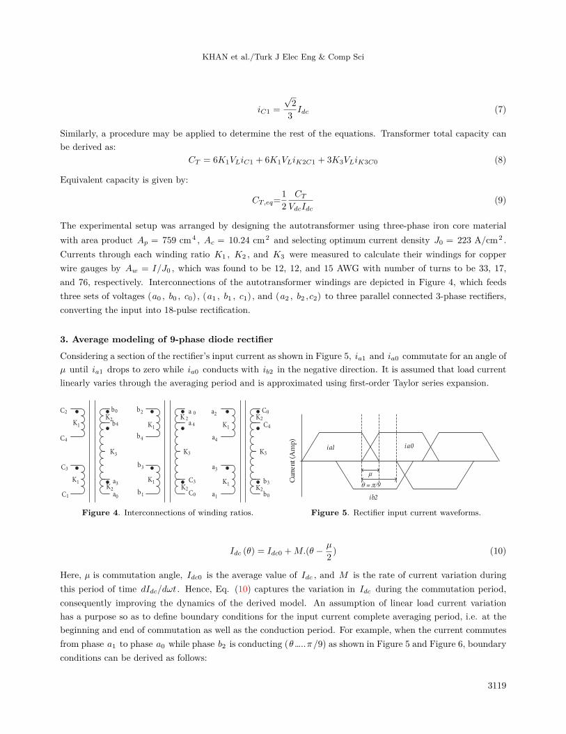
The experimental setup was arranged by designing the autotransformer using three-phase iron core materialwith area product Ap = 759 cm4 , Ac = 10.24 cm2 and selecting optimum current density J0 = 223 A/cm2 .Currents through each winding ratio K1 , K2 , and K3 were measured to calculate their windings for copperwire gauges by Aw = I/J0 , which was found to be 12, 12, and 15 AWG with number of turns to be 33, 17,and 76, respectively. Interconnections of the autotransformer windings are depicted in Figure 4, which feedsthree sets of voltages (a0 , b0 , c0) , (a1 , b1 , c1) , and (a2 , b2 ,c2) to three parallel connected 3-phase rectifiers,converting the input into 18-pulse rectification.

3. Average modeling of 9-phase diode rectifier

Considering a section of the rectifier’s input current as shown in Figure 5, ia1 and ia0 commutate for an angle ofµ until ia1 drops to zero while ia0 conducts with ib2 in the negative direction. It is assumed that load currentlinearly varies through the averaging period and is approximated using first-order Taylor series expansion.

C0

C0

C2

C1

C3

C3

C4

C4

b0

b0b1

b2

b4

b4

b3

b3

a 0

a0

a2

a1

a3

a3

a4

a 4K1

K1

K1

K1

K1

K1

K2

K2

K 2

K2

K2

K2

K3 K3 K3

ia0

ib2

µ

θ = π/9

Current(Amp)

ia1

Figure 4. Interconnections of winding ratios. Figure 5. Rectifier input current waveforms.

Idc (θ) = Idc0 +M.(θ − µ

2) (10)

Here, µ is commutation angle, Idc0 is the average value of Idc , and M is the rate of current variation duringthis period of time dIdc/dωt . Hence, Eq. (10) captures the variation in Idc during the commutation period,consequently improving the dynamics of the derived model. An assumption of linear load current variationhas a purpose so as to define boundary conditions for the input current complete averaging period, i.e. at thebeginning and end of commutation as well as the conduction period. For example, when the current commutesfrom phase a1 to phase a0 while phase b2 is conducting (θ…..π/9) as shown in Figure 5 and Figure 6, boundaryconditions can be derived as follows:

3119


+

-

ia

+

-

ia

a1

b1

c1

Ldc Ldc

Vdc Vdcc1

Ls

Ls

Ls

Ls

Ls

Lsa2

b2

c2

a2

b2

c2

a0

b0

c0c0

b0

a0

a1

b1

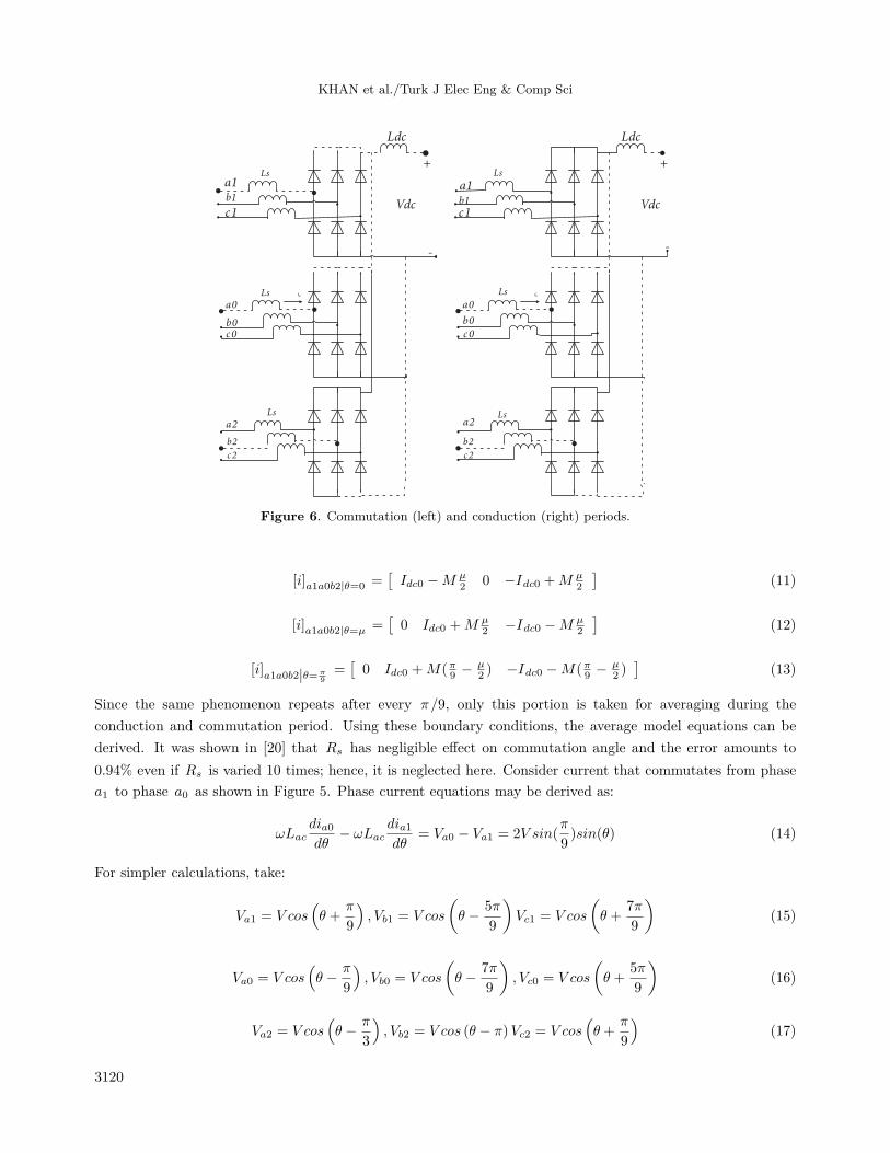
Figure 6. Commutation (left) and conduction (right) periods.

[i]a1a0b2|θ=0 =[Idc0 −M µ

2 0 −Idc0 +M µ2

](11)

[i]a1a0b2|θ=µ =[0 Idc0 +M µ

2 −Idc0 −M µ2

](12)

[i]a1a0b2|θ=π9=[0 Idc0 +M(π9 − µ

2 ) −Idc0 −M(π9 − µ2 )]

(13)

Since the same phenomenon repeats after every π/9, only this portion is taken for averaging during theconduction and commutation period. Using these boundary conditions, the average model equations can bederived. It was shown in [20] that Rs has negligible effect on commutation angle and the error amounts to0.94% even if Rs is varied 10 times; hence, it is neglected here. Consider current that commutates from phasea1 to phase a0 as shown in Figure 5. Phase current equations may be derived as:

ωLacdia0dθ

− ωLacdia1dθ

= Va0 − Va1 = 2V sin(π

9)sin(θ) (14)

For simpler calculations, take:

Va1 = V cos(θ +

π

9

), Vb1 = V cos

(θ − 5π

9

)Vc1 = V cos

(θ +

7π

9

)(15)

Va0 = V cos(θ − π

9

), Vb0 = V cos

(θ − 7π

9

), Vc0 = V cos

(θ +

5π

9

)(16)

Va2 = V cos(θ − π

3

), Vb2 = V cos (θ − π)Vc2 = V cos

(θ +

π

9

)(17)

3120


Integrating Eq. (14) from 0 to θ range including commutation and conduction period:

ia0(θ) =V

ωLacsin(π9

)(1− cos θ) + Mθ

2(18)

For commutation angle derivation, evaluate Eq. (18) at θ = µ.

Idc0 +Mµ

2=

V

ωLacsin(π9

)(1− cosµ) + Mµ

2(19)

Rearranging:

µ = cos−1

(1− Idc0.ωLac

V sin(π9

)) (20)

Similarly: eIb2 (θ)= −Idc0−K

(θ−µ

2

)(4)

ib2 (θ) = −Idc0 −M(θ − µ

2

)(21)

For Ia1(θ) ia1Ia1

(θ) , put ia0 (θ) = Idc (θ)− ia1 (θ) in Eq. (14), and integrate over 0 to θ . Rearrangement gives:

ia1 (θ) = Idc0 −V

ωLacsin(π9

)(1− cos θ) + M

2(θ − µ) (22)

3.1. Output DC voltage and currentThe average value DC link voltage and current over the diode switching period can be obtained using the statespace averaging technique as given in [26]. Circuit equations during commutation and conduction are givenbelow, where Up and eUn represent the voltages of the positive and negative terminals of rectifiers with respectto neutral (n) as shown in Figure 1:

Va0 (t)= Racia0 (t) + Lacdia0(t)

dt + Up

Va1(t)= Racia1 (t) + Lac

dia1(t)dt + Up

Vb2 (t)= Racib2 (t) + Lacdib2(t)

dt + Un

&

ia0 (t) + ia1 (t) = Idc (t)ib2 (t) = −Idc (t)

(23)

Va0 (t)= Racia0 (t) + Lac

dia0(t)dt + Up

Vb2 (t)= Racib2 (t) + Lacdib2 (t)

dt + Un

&

ia0 = Idc (t)

ia1 = 0

ib2 = −Idc (t)

(24)

Similarly at the DC load side:

Up − Un= RdcIdc (t) + LdcdIdc (t)

dt+ Vdc (25)

Solving Eqs. (23) and (24) for Up and Un and putting this in Eq. (25) yields:

dIdc (t)

dt= −R1

L1Idc (t)−

Vb2 (t)

L1

(cos(π9

)+ 1)− Vdc

L1(26)

3121


dIdc (t)

dt= −R2

L2Idc (t) +

Va0 (t)− Vb2 (t)

L2− Vdc

L2(27)

Here, R1 = Rdc +32Rac , L1 = Ldc +

32Lac , R2 = Rdc + 2Rac , L2 = Ldc + 2Lac .

Put the values of Va0 and Vb2 in Eqs. (26) and (27) where θ = ωt and 0 ≤θ≤ 2π . Since input/outputcurrents and voltages repeat after every π

9 rad interval, the dynamic equation for Idc during conduction andcommutation may be expressed as:

dIdcdt = −R1

L1Idc (α) +

VL1

(cos(π9

)+ 1)

cos (α)− Vdc

L1

dIdcdt = −R2

L2Idc (α) +

V (cos (π9 )+1) cos(α)+V sin (α) sin(π

9 )L2

− Vdc

L2

0 ≤ α < µ

µ ≤ α < π9

(28)

Here, 0 ≤ α < θ −m(π9

)< π

9 , m=1,2,3….For establishing a time-invariant model, a state-space average technique is applied as:

⟨x⟩0 (t) =1

T

∫ t

t−T

x (τ) dτ

For a periodic, time-dependent state-space equation:

dx (t)

dt= f x (t) , u (t)

When the average value is taken as the state variable, the time derivative of the average is given by:

d⟨x⟩0(t)dt

= ⟨dxdt

⟩0(t) = ⟨f(x, u)⟩0

Hence:

dIDC

dt=9

π

[((R2

L2− R1

L1

)µ− πR2

9L2

)Idc0 −

R2

L2M

(π2

162− µπ

18

)+

((1

L2− 1

L1

)µ− π

9L2

)Vdc

+V

(1

L1− 1

L2

)(cos(π9

)+ 1)

sin (µ) +V

L2sin(π9

)(cos (µ) + 1)

](29)

3.2. AC currents

The conventional dq0 transformation cannot be applied for the AC input currents as a 9-phase rectifier is beingused. In order to scale the 9-phase dq0 space into 3-phase dq0 space, a constant multiplying factor is used sothat the converter active power remains the same in 3-phase and 9-phase dq0 frames. It is required to apply

3122


9-phase transformation into the dq0 synchronous reference frame as:

T 9dq =

1

3

√2

3

cos (θ + π9 ) sin (θ + π

9 )

cos (θ − 5π9 ) sin (θ − 5π

9 )

cos (θ + 7π9 ) sin (θ + 7π

9 )

cos (θ − π9 ) sin (θ − π

9 )

cos (θ − 7π9 ) sin (θ − 7π

9 )

cos (θ + 5π9 ) sin (θ + 5π

9 )

cos (θ − π3 ) sin (θ − π

3 )

cos (θ − π) sin (θ − π)

cos (θ + π3 ) sin (θ + π

3 )

T

(30)

During the averaging period the only involved phases (shown in Figure 5) are ia0 , ia1 , and ib2 , so in the dq0synchronous reference frame:

[idiq

]=

√2

3√3

[cos (θ − π

9 ) cos (θ + π9 ) cos (θ − π)

− sin (θ − π9 ) − sin (θ + π

9 ) − sin (θ − π)

] ia0ia1ib2

(31)

Integrating the above equations for average values id and iq during commutation and conduction periodsseparately and averaging over period π/9 π

9 yields:

id =

√6

π

[V

2ωLsin2

(π9

)(cos (2µ)− 4 cos (µ)+3) + 2Idc0 sin

(π9

)cos (µ) +M sin

(π9

)(π9− sin (µ)

)](32)

and

iq =−√6

π

[V

2ωLsin2

(π9

)(sin (2µ)− 4 sin (µ) + 2µ) + 2Idc0 sin (µ) sin

(π9

)+M

(sin(π9

)(1 + cos (µ))− π

9− π

9cos(π9

))](33)

Eqs. (29), (32), and (33) represent the complete average model for the 9-phase diode rectifier where M accountsfor the dynamics of the load current.

4. Simulations and experimental results

Vc2= V cos(θ+π9 )In this section, simulation results are compared with those of hardware, with converter spec-

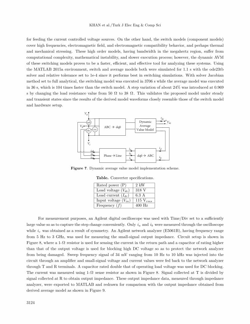
ifications given in the Table and circuit parameters in the Appendix, for validation. Implementation of theproposed dynamic average model in Simulink is shown in Figure 7 where a three-phase supply system is trans-formed into a dq0 synchronous reference frame and fed to the derived model equations. The output DC voltageis fed to the load, which draws the required amount of current from the supply. Currents id and iq are trans-formed into phase currents through dq0 to ABC conversion, which are further transformed into line currents

3123


for feeding the current controlled voltage sources. On the other hand, the switch models (component models)cover high frequencies, electromagnetic field, and electromagnetic compatibility behavior, and perhaps thermaland mechanical stressing. These high order models, having bandwidth in the megahertz region, suffer fromcomputational complexity, mathematical instability, and slower execution process; however, the dynamic AVMof these switching models proves to be a faster, efficient, and effective tool for analyzing these systems. Usingthe MATLAB 2015a environment, switch and average models both were simulated for 1.1 s with the ode23tbsolver and relative tolerance set to 1e-4 since it performs best in switching simulations. With solver Jacobianmethod set to full analytical, the switching model was executed in 3706 s while the average model was executedin 36 s, which is 104 times faster than the switch model. A step variation of about 24% was introduced at 0.969s by changing the load resistance value from 50 Ω to 38 Ω . This validates the proposed model under steadyand transient states since the results of the derived model waveforms closely resemble those of the switch modeland hardware setup.

ABC → dq0

Dynamic Average

Value Model

dq0 → ABCPhase → Line

iab

icaibc

Va

Vb

Vc

iabibcica

ia

ib

ic

Vdc

Idc+-

id

iq

Figure 7. Dynamic average value model implementation scheme.

Table. Converter specifications.

Rated power (P) 2 kWLoad voltage (Vdc) 318 VLoad current (Idc) 6.3 AInput voltage (Vin) 115 Vrms

Frequency (f) 400 Hz

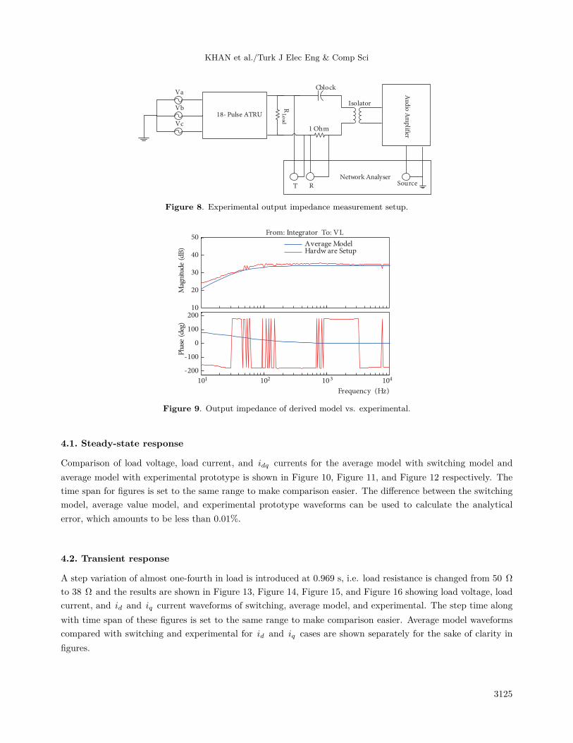
For measurement purposes, an Agilent digital oscilloscope was used with Time/Div set to a sufficientlylarge value so as to capture the step change conveniently. Only ia and ib were measured through the oscilloscopewhile ic was obtained as a result of symmetry. An Agilent network analyzer (E5061B), having frequency rangefrom 5 Hz to 3 GHz, was used for measuring the small-signal output impedance. Circuit setup is shown inFigure 8, where a 1-Ω resistor is used for sensing the current in the return path and a capacitor of rating higherthan that of the output voltage is used for blocking high DC voltage so as to protect the network analyzerfrom being damaged. Sweep frequency signal of 34 mV ranging from 10 Hz to 10 kHz was injected into thecircuit through an amplifier and small-signal voltage and current values were fed back to the network analyzerthrough T and R terminals. A capacitor rated double that of operating load voltage was used for DC blocking.The current was measured using 1-Ω sense resistor as shown in Figure 8. Signal collected at T is divided bysignal collected at R to obtain output impedance. These output impedance data, measured through impedanceanalyzer, were exported to MATLAB and redrawn for comparison with the output impedance obtained fromderived average model as shown in Figure 9.

3124


Va

Vb

Vc

18- Pulse ATRU

Au

dio A

mp

lifier

Network Analyser

T R Source

RLo

ad

Isolator

1 Ohm

Cblock

Figure 8. Experimental output impedance measurement setup.

Frequency (Hz)

Ph

ase

(deg

)M

agn

itud

e (d

B)

101 102 103 104

-200

-100

0

100

20010

20

30

40

50From : Integrator To: VL

Average ModelHardw are Setup

Figure 9. Output impedance of derived model vs. experimental.

4.1. Steady-state response

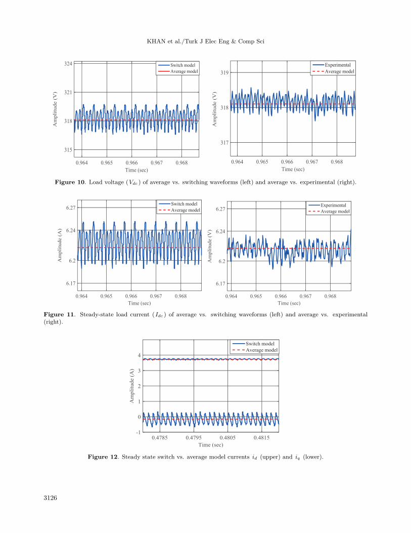
Comparison of load voltage, load current, and idq currents for the average model with switching model andaverage model with experimental prototype is shown in Figure 10, Figure 11, and Figure 12 respectively. Thetime span for figures is set to the same range to make comparison easier. The difference between the switchingmodel, average value model, and experimental prototype waveforms can be used to calculate the analyticalerror, which amounts to be less than 0.01%.

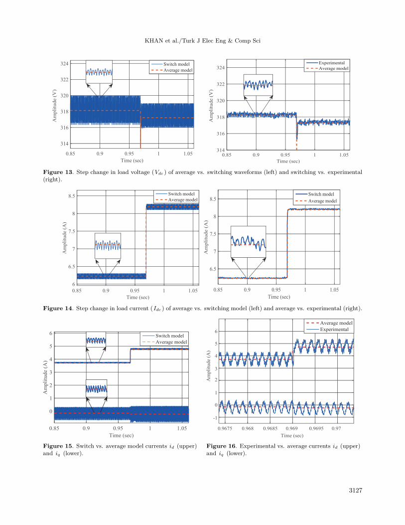
4.2. Transient response

A step variation of almost one-fourth in load is introduced at 0.969 s, i.e. load resistance is changed from 50 Ω

to 38 Ω and the results are shown in Figure 13, Figure 14, Figure 15, and Figure 16 showing load voltage, loadcurrent, and id and iq current waveforms of switching, average model, and experimental. The step time alongwith time span of these figures is set to the same range to make comparison easier. Average model waveformscompared with switching and experimental for id and iq cases are shown separately for the sake of clarity infigures.

3125


Figure 10. Load voltage (Vdc ) of average vs. switching waveforms (left) and average vs. experimental (right).

Figure 11. Steady-state load current (Idc ) of average vs. switching waveforms (left) and average vs. experimental(right).

Figure 12. Steady state switch vs. average model currents id (upper) and iq (lower).

3126


Figure 13. Step change in load voltage (Vdc ) of average vs. switching waveforms (left) and switching vs. experimental(right).

Figure 14. Step change in load current (Idc ) of average vs. switching model (left) and average vs. experimental (right).

Figure 15. Switch vs. average model currents id (upper)and iq (lower).

Figure 16. Experimental vs. average currents id (upper)and iq (lower).

3127


5. ConclusionsThis paper proposed an effective mathematical average modeling and evaluation of 18-pulse diode rectifiers thatare used for impedance extraction, stability measurements, and analysis. Switching models are discontinuous,complex, and nonlinear in behavior and hence cause mathematical instability as well as consume more time inexecution. The proposed explicit mathematical average model converts the switching model into continuous soas to run orders of magnitudes faster than the original switching model. This allow computationally efficientanalysis of relatively slower dynamics such as those involved in the destabilizing phenomena that may arisedue to the interaction between tightly regulated loads and energy storage components. Avoiding mathematicalinstability problems makes its applications twofold. Waveforms and results of the derived model as well as theprototype and switching model, under steady state as well as dynamic state, are in close agreement. Hence, thederived model can be used for linearization and small-signal output impedance extraction for stability analysis,which is the key advantage.

References

[1] Sarlioglu B, Morris CT. More electric aircraft: review, challenges, and opportunities for commercial transportaircraft. IEEE T Trans Electr 2015; 1: 54-64.

[2] Yang T, Bozhko S, Asher G. Functional modeling of symmetrical multipulse autotransformer rectifier units foraerospace applications. IEEE T Power Electr 2015; 30: 4704-4713.

[3] Szczesniak P, Urbanski K, Fedyczak Z, Zawirski K. Comparative study of drive systems using vector-controlledPMSM fed by a matrix converter and a conventional frequency converter. Turk J Elec Eng & Comp Sci 2016; 24:1516-1531.

[4] Yu Z, Fu L, Zhu X, Ngoc T, Wen Z. Operational characteristics of a filtering rectifier transformer for industrialpower systems. Turk J Elec Eng & Comp Sci 2013; 21: 1272-1283.

[5] Singh B, Singh S, Hemanth CSP. Power quality improvement in load commutated inverter-fed synchronous motordrives. IEEE T IET Power Electr 2010; 3: 411-428.

[6] Chaturvedi PK, Jain S, Pradhan KC, Goyal V. Multi-pulse converters as a viable solution for power qualityimprovement. In: IEEE 2006 Power India Conference; June 2006; Vidisha, India. New York, NY, USA: IEEE.pp. 6-11.

[7] Derek PA. Power Electronic Converter Harmonic Multipulse Methods for Clean Power. 1st ed. New York, NY,USA: Wiley, 1996.

[8] Cross A, Baghramian A, Forsyth A. Approximate, average, dynamic models of uncontrolled rectifiers for aircraftapplications. IET T Power Electr 2009; 2: 398-409.

[9] Lo Calzo G, Zanchetta P, Gerada C, Lidozzi A, Degano M, Crescimbini F, Solera L. Performance evaluation ofconverter topologies for high speed starter/generator in aircraft applications. In: IEEE 2014 Industrial ElectronicsSociety Annual Conference; 29 October–1 November 2014; Dallas, TX, USA. New York, NY, USA: IEEE. pp.1707-1712.

[10] Yang T, Bozhko S, Asher G. Modeling of uncontrolled rectifiers using dynamic phasors. In: IEEE 2012 ElectricalSystems for Aircraft, Railway and Ship Propulsion; 16–18 October 2012; Bologna, Italy. New York, NY, USA:IEEE. pp. 1-6.

[11] Yang T, Bozhko S, Asher G. Modeling of active front-end rectifiers using dynamic phasors. In: IEEE 2012International Symposium on Industrial Electronics; 28–31 May 2012; Hangzhou, China. New York, NY, USA:IEEE. pp. 387-392.

[12] Chiniforoosh S, Hamid A, Juri JA. Generalized methodology for dynamic average modeling of high-pulse-countrectifiers in transient simulation programs. IEEE T Energy Conv 2016; 31: 228-239.

3128


[13] Huang J, Corzine KA. AC impedance measurement by line-to-line injected current. In: IEEE 2006 Conference onIndustry Applications Conference Forty-First IAS Annual Meeting; 8–12 October 2006; Tampa, FL, USA. NewYork, NY, USA: IEEE. pp. 300-306.

[14] Yang T, Bozhko S, Asher G. Fast functional modelling of diode-bridge rectifier using dynamic phasors. IET T PowerElectr 2015; 8: 947-956.

[15] Chiniforoosh S, Hamid A, Davoudi A, Jatskevich J, Martinez JA, Saeedifard M, Aliprantis DC, Sood VK. Steady-state and dynamic performance of front-end diode rectifier loads as predicted by dynamic average-value models.IEEE T Power Del 2013; 28: 1533-1541.

[16] Yang T, Bozhko S, Le-Peuvedic JM, Asher G, Hill CI. Dynamic phasor modeling of multi-generator variablefrequency electrical power systems. IEEE T Power Syst 2016; 31: 563-571.

[17] Chiniforoosh S, Jatskevich J, Dinavahi V, Iravani R, Martinez JA, Ramirez A. Dynamic average modeling of line-commutated converters for power systems applications. In: IEEE Power & Energy Society General Meeting; 26–30July 2009; Calgary, Canada. New York, NY, USA: IEEE. pp. 1-8.

[18] Chiniforoosh S, Jatskevich J, Yazdani A, Sood V, Dinavahi V, Martinez JA, Ramirez A. Definitions and applicationsof dynamic average models for analysis of power systems. IEEE T Power Del 2010; 25: 2655-2669.

[19] Ebrahimi S, Amiri N, Atighechi H, Jatskevich J, Wang L. Parametric average value modeling of high power AC/ACcyclo converters. In: IEEE 2015 16th Workshop on Control and Modeling for Power Electronics; 12–15 July 2015;Vancouver, Canada. New York, NY, USA: IEEE. pp. 1-6.

[20] Zhu H. New multipulse diode rectifier average models for AC and DC power systems studies. PhD, VirginiaPolytechnic Institute, Blacksburg, VA, USA, 2005.

[21] Maldonado MA, Shah NM, Cleek KJ, Walia PS, Korba GJ. Power management and distribution system for amore-electric aircraft (MADMEL) – program status. In: IECEC-97 Proceedings of the Thirty-Second IntersocietyEnergy Conversion Engineering Conference (Cat. No. 97CH6203). pp. 3-8.

[22] Burleson C, Maurice L. Aviation and the environment: challenges and opportunities. In: AIAA/ICAS 2003International Air and Space Symposium and Exposition; 14–17 July 2003; Dayton, OH, USA. pp. 1-11.

[23] Griffo A, Wang J. State-space average modelling of synchronous generator fed 18-pulse diode rectifier. In: IEEE2009 13th Conference on Power Electronics and Applications; 8–10 September 2009; Barcelona, Spain. New York,NY, USA: IEEE. pp. 1-10.

[24] Shahbaz K, Hui GZ, Husan A, Kashif H, Izhar UH. Comparative analysis of differential delta configured 18-pulseATRU. In: IEEE 2015 International Conference Electrical Systems for Aircraft, Railway, Ship Propulsion and RoadVehicles; 3–5 March 2015; Aachen, Germany. New York, NY, USA: IEEE. pp. 1-6.

[25] Kuniomi O. Autotransformer-based 18-pulse rectifiers without using DC-side interphase transformers: classificationand comparison. In: IEEE 2008 International Symposium on Power Electronics, Electrical Drives, Automation andMotion; 11–13 June 2008; Ischia, Italy. New York, NY, USA: IEEE. pp. 760-765.

[26] Han L, Wang J, Howe D. State-space average modelling of 6- and 12-pulse diode rectifiers. In: IEEE 2007 PowerElectronics and Applications European Conference; 2–5 September 2007; Aalborg, Denmark. New York, NY, USA:IEEE. pp. 1-10.

3129


Appendix

Parameters:

Lp = 100 µH, RS = 1.75 mΩ

Ls = 0.55 mH Rdc = 235 mΩ

Ldc = 3 mH Lac = Ls + Lp×nv ×ni

Rp = 7.97e-6 Ω Ron = 1 mΩ

1

Documents

Average modeling and evaluation of 18-pulse