Embed Size (px)
Citation preview


MFA-MANUAL (Vers. 1.91)
Guidelines for the Use of Material Flow Analysis
(MFA) for Municipal Solid Waste (MSW) Management
Project AWAST Aid in the Management and European Comparison of Municipal Solid WASte Treat-
ment methods for a Global and Sustainable Approach
Contract number. EVK4-CT-2000-00015
Workpackage 1 Waste matter aspects
(Waste characterisation - Systems definition and data processing) (D1, D2)
Roland Fehringer, Bernd Brandt, Paul H. Brunner Vienna University of Technology Institute for Water Quality and Waste Management
Hans Daxbeck, Stefan Neumayer, Roman Smutny Resource Management Agency
Jacques Villeneuve, Pascale Michel Bureau de Recherches Géologiques et Miniéres
University of Stuttgart Martin Kranert, Andrea Schultheis, Dieter Steinbach Stuttgart University Institute for Water Quality and Waste Management

University of Stuttgart
AWAST D1 – D2: MFA Manual i
Table of contents
1 Introduction .........................................................................................................1
1.1 Objectives of the AWAST Project .................................................................1
1.2 Objectives of the MFA Manual......................................................................1
2 Introduction to Material Flow Analysis (MFA) ..................................................3
2.1 History of MFA and Fields of Application......................................................4
3 The Methodology of MFA ...................................................................................9
3.1 Terms and Definitions.................................................................................10
3.2 Procedures .................................................................................................12
3.2.1 Objectives and Questions...............................................................12
3.2.2 System Definition ...........................................................................13
3.2.2.1 System Boundary ........................................................................15
3.2.2.2 Definition of Processes and Goods..............................................15
3.2.2.3 Subsystems .................................................................................18
3.2.2.4 Selection of Substances ..............................................................19
3.2.3 Rough assessment of Balance.......................................................21
3.2.3.1 Rough Collecting and Processing of Data ...................................22
3.2.3.2 Rough balancing..........................................................................22
3.2.3.3 Sensitivity analysis.......................................................................22
3.2.4 Planning and Performance of a Research or Measurement Programme.....................................................................................23
3.2.5 Goods Fluxes Calculation ..............................................................23
3.2.6 Transfer Function and Transfer Coefficients Calculation................24
3.3 Results Presentation and interpretation......................................................25
3.3.1 Tables and Graphs.........................................................................25
4 Application of MFA in Waste Management.....................................................29
4.1 Objectives of the Waste Management........................................................29
4.2 The importance of MFA for the Objectives of the Directive on Waste ........32
4.2.1 Fulfilling the Objectives of the Directive on Waste (DoW) ..............32
4.2.2 Measures for a Better Fulfilment of the DoW Objectives................33
4.2.3 Efficiency of Measures ...................................................................34
University of Stuttgart
AWAST D1 – D2: MFA Manual ii
4.2.4 Forecasting.....................................................................................34
4.2.5 Monitoring.......................................................................................35
4.3 Capacity of MFA towards Waste Management...........................................35
4.4 Assessment of Material Balances...............................................................37
4.4.1 Limit Values....................................................................................37
4.4.2 Comparing geogenic to anthropogenic flows and stocks ...............37
4.4.3 Critical Volume ...............................................................................38
4.4.4 Substance Concentration Efficiency (SCE) ....................................39
4.4.5 Material Input per Service Unit (MIPS) ...........................................39
4.4.6 Life Cycle Assessment (LCA).........................................................40
4.5 Materials Accounting ..................................................................................40
5 Determination of the composition of municipal solid waste.........................43
5.1 Introduction.................................................................................................43
5.1.1 Definition of Municipal Solid Waste ................................................43
5.1.2 Objectives of Waste Analysis .........................................................43
5.2 Approach ....................................................................................................43
5.2.1 The Life Cycle of a Good................................................................43
5.3 Waste Analysis Methods ............................................................................44
5.3.1 Direct Analysis................................................................................44
5.3.1.1 Description of the method used in France ...................................45
5.3.1.1.1 Sampling methodology .............................................................45
5.3.1.1.2 Sorting and Analyzing of the Waste Samples...........................47
5.3.1.2 Description of the method used in Austria ...................................50
5.3.1.2.1 Sampling methodology .............................................................50
5.3.1.2.2 Sorting and analysing of the waste samples ............................51
5.3.1.3 Potentials and limitations of direct analysis..................................52
5.3.2 Waste analysis with market research data .....................................52
5.3.2.1 Description of the method ............................................................52
5.3.2.2 Application of the method to packaging glass..............................55
5.3.2.3 Application of the method to the substance chlorine....................57
5.3.2.4 Potentials and limits of the market product analysis ....................58
5.3.3 Analysis of waste treatment products.............................................59
5.3.3.1 Description of the method ............................................................59

University of Stuttgart
AWAST D1 – D2: MFA Manual iii
5.3.3.2 Online monitoring system ............................................................61
5.3.3.3 Potentials and limitations of the analysis of waste treatment products .......................................................................................65
5.4 Conclusions ................................................................................................66
6 Examples ...........................................................................................................67
6.1 Thermal Treatment .....................................................................................67
6.1.1 Waste Incineration in Grate Furnace Incinerators ..........................67
6.1.1.1 Functioning of a Waste Incineration Plant (Vienna, Spittelau) .....68
6.1.1.2 MFA of a Waste Incineration Plant (Vienna, Spittelau) ................70
6.1.2 Industrial Incineration by means of a Fluidised Bed Plant ..............70
6.1.2.1 Functioning of Fluidised Bed Incineration Plant ...........................72
6.1.2.2 MFA of a Fluidised Bed Incineration Plant (Austria, RVL-Lenzing73
6.1.3 Industrial Incineration by means of Rotary Shaft Kilns (Cement Industry) .........................................................................................73
6.1.3.1 Functioning of a Heat Exchange Rotary Kiln Shaft in the Cement Industry ........................................................................................74
6.1.3.2 MFA of a Rotary Kiln Shaft for Cement Production (Austria, Mannersdorf) ...............................................................................75
6.2 Mechanical Biological Waste Treatment.....................................................76
6.2.1 Introduction.....................................................................................76
6.2.1.1 Functioning of a Facility for Mechanical Biological Waste Treatment ....................................................................................76
6.2.1.2 Legal Framework in Europe.........................................................77
6.2.2 Case Study Aerobic Mechanical Biological Treatment of Residual Wastes (Residual Waste Treatment Plant Allerheiligen - Austria)..78
6.2.2.1 System Definition.........................................................................79
6.2.2.2 Determining the Goods and Substance Fluxes............................81
6.2.2.3 Results for the Allerheiligen Plant for mechanical biological treatment......................................................................................82
6.2.2.4 Conclusions .................................................................................83
6.2.2.5 Average transfer coefficients of a plant for mechanical biological treatment......................................................................................83
6.2.3 Case Study Anaerobic Mechanical Biological Treatment of Residual Wastes ...........................................................................................84
6.2.3.1 Technology Variants of Anaerobic Treatment..............................84
6.2.3.2 Pilot Plant of the Provincial County of Ravensburg, Germany.....88
University of Stuttgart
AWAST D1 – D2: MFA Manual iv
6.2.3.3 Model Derived from the Münster PMBWT, Germany...................89
6.2.3.4 Fermentation of Mechanically Pre-treated Household Wastes in Lab Conditions.............................................................................90
6.2.3.5 Transfer Coefficients of an Anaerobic Treatment Plant by the BTA Enterprise ....................................................................................91
6.2.3.6 Conclusions for the Anaerobic Plant ............................................92
6.3 Landfill 92
6.3.1 Introduction.....................................................................................92
6.3.1.1 Legal Framework in Europe (The Landfill Directive) ....................92
6.3.2 Case Study Landfill ........................................................................92
6.3.2.1 System Definition.........................................................................92
6.3.2.2 Estimation of the goods and elemental fluxes..............................94
6.3.2.3 Results.........................................................................................97
7 Literature ...........................................................................................................99
University of Stuttgart
AWAST D1 – D2: MFA Manual 1
1 Introduction
The MFA Manual is the deliverable D2 and the chapter 5 (methods to determine the compo-sition of waste) is the deliverable D1 of the project AWAST - Workpackage 1. 1.1 Objectives of the AWAST Project
Municipal solid waste (MSW) management is a major problem for all communities of the EU. The different actors involved (policymakers, industry, municipalities) are facing a lack of methodology and software for defining, evaluating, optimising or adapting their waste treat-ment decisions and for meeting the progress targets set at the EU level. The AWAST project objective is to meet this need by providing end-users and stakeholders with a flexible decision support tool that, in a comprehensive approach, takes into account technical, energetic and economic aspects, and also the social and environmental issues. The objectives for this decision support tool are:
Flexibility Adaptability to local context Simulation Process analysis as background Application of the experience of Central and Western EU countries Consideration of energetic and economic aspects within the whole waste management
system. The aim of this decision support tool is to enable cities and industrial operators involved in city waste management, possibly throughout the European Community, to:
evaluate present situation in terms of waste processing efficiency, cost, energetic bal-ance, residual streams, etc.
investigate alternative MSW management paths, accompany, control and reorient the choices, define and plan sustainable degrees of progress, and improve the concept implementation of an integrated municipal solid waste manage-
ment. The project objectives are addressed by a work plan comprising 10 work packages (WP). 1.2 Objectives of the MFA Manual
This manual follows the objectives of the project and the “description of work” given in work package 1 (WP1). WP1 focuses on waste matter description and has two tasks to solve:
University of Stuttgart
AWAST D1 – D2: MFA Manual 2
• Characterisation of the waste input into the waste management system in terms of quan-tity and quality. Development of three different approaches to determine the waste and product input: direct analysis, analysis of waste treatment product and analysis of market research data. (Chapter 5)
• Definition of the data structure of the entire project based on the methodology of material
flux analysis (MFA). This data structure serves as a powerful tool for co-ordinating all the modules of the project, linking together the work of all partners and reconciliating the data of the sub-projects. Transfer of know-how on the MFA methodology. (Chapters 2 - 4, 6, 7)
The objectives of this manual are to determine and provide the project partners with: • a rigid methodology to establish mass balances of municipal waste management sys-
tems, • a basic, common terminology for system and process analysis of municipal waste man-
agement systems, • waste characterisation methods (direct analysis, analysis of waste treatment products
and analysis of market research data), • MFA case studies, • system analysis of municipal solid waste management for the simulator.

University of Stuttgart
AWAST D1 – D2: MFA Manual 3
2 Introduction to Material Flow Analysis (MFA)
Material Flow Analysis (MFA) method enables the description of systems of any complexity grade. It allows for depicting not only operational processes, cities, regions, nations but also entities such as the EU. The advantage of the Material Flow Analysis is the possibility for reducing complex systems to the key goods and processes relevant fort he study objectives. This way, the base is created for deriving necessary measures or for calculating scenarios aiming at system optimisation. By elaborating the method at the end of the eighties, together with a determined regulated methodical approach, a special “language” was adopted as well [Baccini & Brunner, 1991]. From the very beginning, the goal has been to develop a tool being as universally applicable as possible and, when applied in different studies, the results being comparable to each other. This unified common language makes it easier to link systems both at horizontal and vertical levels. An example for a horizontal linking is connecting the substance flows of two neighboured regions. By a vertical linkage, the substance flows of an enterprise are inte-grated into the ones of the surrounding region. The key terms used most often when carrying out Material Flow Analyses are: system boundary, process, goods and substance. Defining the “System boundary” is the initial point of every MFA. The decision is to be made which processes are to be considered within the system and which not. This is indi-cated as defining the system boundary. At the same time, a system boundary in time is to be set as well, i.e. the time period for which the balance is performed. It usually amounts to one year. Parallel to defining the system boundary, the processes to consider are determined. The term „Process” stands for transportation, storage or transformation of goods and sub-stances. The process itself is usually regarded as a “black box”, i.e. internal development is not investigated except the case when the process contents a stock. Here, the stock mass and is change are taken into account. Processes are connected to each other by goods and substance fluxes, and every flux has a process of origin and a destination process. A „Good“ is defined as a tradable matter con-sisting of one pr several substances So for example, drinking water and PVC are goods, since drinking water contains dissolved substances, and the vinyl chloride in the PVC is pre-treated with additives. The trade value of the goods can be both positive (e.g. bread, flour, vegetables, drinking water, batteries, scrap metal) and negative (e.g. solid waste, old batter-ies, wastewater). Thus, goods are built of substances. A “Substance” is defined as a chemical element or compound in its pure form. Examples for substances are carbon, oxygen, hydrogen, chlorine, zinc, cadmium, and compounds, zinc oxide (ZnO), benzene, glucose(C6H12O6), water (H2O),chloroethene (= vinylchloride).

University of Stuttgart
AWAST D1 – D2: MFA Manual 4
2.1 History of MFA and Fields of Application
Although the Material Flow Analysis method was developed relatively a short time ago, the attempts to describe system metabolism and to elaborate input-output analyses go far back in time. This chapter gives an overview over the history of the material flow analysis. Finally, a demonstration of the practical application of the method is made. Human Metabolism Already in the 17th century the Venetian doctor Santorio Santorio undertook numerous ex-periments to enable describing the human metabolism. When performing balances of the amount of food intake and the excrements emitted, he established a (measurable) deficit on the part of the output of the human body. Thus, he concluded that part of the food must have been emitted by sort of an “invisible sweating”. Just several years of experimental work en-abled Santorio Santorio to calculate the amount lost by the invisible sweating in function of the visible excretions and a variety of internal and external factors [Major, 1938]. Introducing the method of balancing systems helped the science investigate the human me-tabolism. Since it was Santorio who first took up the idea of constructing balances and per-formed practical experiments, he is considered the father of the metabolism sciences. Santorio’s results are still up-to-date: nowadays, it is necessary to investigate the metabolism of the anthroposphere. For instance, the diffuse, uncontrolled emissions of metals during corrosion are equally little perceptible, and thus an equal challenge, for us as the phenome-non of the invisible sweating was 400 years ago. Whereas human sweat normally hides no threat, diffusive emissions from the anthroposphere could possibly do, for both human and environment. As once constructing balances of goods lead to the secret of the internal hu-man metabolism, we currently face the task to understand the metabolism of the organism “anthroposphere“ [Merl, 1996]. Identifying the Origin of Environmental Problems – a Way Out of the End-of-Pipe Solutions Ayres and Kneese suggested 1969 to construct a substance balance of the entire economic system as a reasonable tool to control and avoid environmental pollution [Ayres & Kneese, 1969]. This idea found its practical application just by Frank Smith within the framework of his dissertation dedicated to investigating the effects of waste landfilling. This way, the first step has been away from end-of-pipe technology set and towards an early recognition of envi-ronmental problems. In the beginning of the seventies, at conferences of the United Nations (UN) the relevance of statistical methods was recognised on substance level. So, 1973 scientist of statistics set the elements of an environmental statistical system, and in the year to follow, the structure of the system and the database were set aiming at an environmental monitoring [United Nations, 1974]. However, this programme has been only partly applied due to limited funding. Investigation of Regional (Urban) Metabolism An ever-increasing part of the population lives in cities. Therefore, long–term safeguarding this living space in a state worth living for its inhabitants is growing to a steadily rising con-cern. Investigating the system “City” proves specific legitimacies of this living space.
University of Stuttgart
AWAST D1 – D2: MFA Manual 5
An example for the begin of the research on the metabolism of cities is given by the Belgian capital Brussels. This study concludes on the significant differences between natural and urban eco systems. Energy, nutrient and water supply occur mainly outwards. These fluxes take other routes than in a natural eco system. The concentrated emission of organic sub-stances over air and wastewater results in a significant pollution of the surrounding environ-ment and the city itself. For this study, the city of Brussels was subdivided into several subsystems classified upon their grade of park facilities, infrastructure and the sociological typology of the inhabitants. An energy balance (including solar energy and energy content of the food) and a water balance were constructed. The biomass (humans, animals, plants) and its increase (by photosynthe-sis) were calculated. On the side of the output, air pollution sources as well as amount and composition for solid wastes and wastewater were determined. The conclusions drawn from both balances were that the anthropogenic eco system “city” in fact does not utilise its own resources and thus “loses” large amounts of materials without having used them. A change of the urban structure is only possible if the urban metabolism is investigated, and the latter can be achieved only by means of interdisciplinary approaches [Duvigneaud & Denayeyer-De Smet, 1975]. At the example of Hong Kong in 1978, the resource intensity of urbanisation in development countries was studied. It was assumed that until the new millennium, ca. 5000 cities world-wide would significantly grow as a consequence of the immigration from their surroundings. If this process develops following the conventional European model, global effects should be expected with regard to material and energy consumption. Hong Kong proves an extremely high population density and a living standard comparable to the one of the industrial nations. The per-capita consumption of raw materials and energy for feeding the infrastructure is however 10 times lower than in the developed countries. The study delivers an overview towards energy, nutrients and drinking water demand. When calculating the energy demand for transportation, the 4 times higher energy input for manu-facturing the transport means. As for the nutrients, a suggestion for their optimal circuit man-agement is elaborated. The stock mass in the infrastructure is broken down with regard to the construction material groups used. The following issues are evaluated: air pollution through transportation and waste incineration plants, soil and ground pollution resulting from resource exploitation, erosion and waste landfilling, and sea quality deterioration through its exploitation for fishing, leisure activities and wastewater inflows. Future urban management strategies should, on the one hand, secure human welfare, but on the other hand, reduce the dependency on external resource supply. This way, stability, di-versity and buffer capacity of urban eco systems can be augmented. The authors of the study conclude that progressive urbanisation presents a very resource intensive process. In order to guarantee a safe and stable supply with energy and goods in the future as well, natural ventilation, heating, cooling etc. processes should be optimally engaged. Only this way the life quality for poor population groups can be improved as well. The key criterion for finding the right solutions is the knowledge of urban metabolism [Newcombe, 1978]. Nations on the Quest for pollutants and Resources by Applying the MFA In the seventies and eighties, balances of goods and substance were calculated in some countries, so to locate the own resource potential, or to determine the environmentally com-

University of Stuttgart
AWAST D1 – D2: MFA Manual 6
patible amounts for dangerous substances. This is the reason for larger regions or even en-tire countries to be often regarded as study objectives. So, for example, a system for balancing the “natural heritage” was developed in France. This balance of goods includes a monetary evaluation of the stock, utilisation and damage of natural resources, and complements the balances of mere physical categories. The goods are divided into “not renewable” (e.g. fossil fuels, oars, sand), “physical environmental sys-tems” (e.g. soil, water) and “living organisms” (animals, plants, microorganisms) and then considered as balances within different eco systems (e.g. forest, pasture, sea) or utilisation sectors (e.g. industry, household). This approach, not translated into the practice yet, could deliver, along with an adjusted information system for it, the base needed for a national sub-stance accounting [Ministry of Housing Physical Planning and the Environment, 1992]. Norway applied a similar goods classification as France, so to calculate balances for the re-sources on stock and to trace their flows. In Sweden and Finland, material flow analyses were elaborated on national level in the sev-enties, whose main focus was on the heavy metals, such as Cd, Hg, Pb. However, some organic compounds were considered as well, e.g. tri-chlorine ethane, tri-butyl tin acetate. In Austria, a substance balance for the heavy metals cadmium (Cd) and lead (Pb) was calcu-lated in 1982. The impulse for this investigation was given by the aim at achieving an in-crease of the recycling rates of both metals. The life cycle of the metals was assessed, from their mining over processing and consumption to disposal. The results showed an unexpect-edly high relevance to be granted to dissipative processes, respectively, to the application of these metals with regard to the metabolism 1 [Jeneral, 1984]. In the beginning of the eighties, the National Oceanographic and Atmospheric Agency (NOAA) of the USA assigned the order for determining the pollutant freights in the Hudson-Raritan Basin. The objective was to trace the effects of the emissions from the last 100 years on the river system. Substance balances were complemented by hydrological substance transportation models, so to depict the substance fluxes within the water body. By consider-ing the registries of the economical activities in the past, the substance cycle for each inves-tigated chemical was described. Also, the processes of production, utilisation and the natural transformation processes were taken into account. The compounds studies were heavy met-als, pesticides and herbicides as well as other critical substances, such as PCB, PAH, oil, P, N, TOC. When regarding the emitters, a differentiation was made between punctual and non-punctual sources. The study proves that substance balances allow for compensating for data material missing and thus to extract the maximal possible use of the data available. A suc-cessful differentiation according to emission sources and utilisation sectors (e.g. agriculture) could be carried out. The results also enabled to prepare a forecast in dependence on fac-tors like land utilisation, population development or emission regulations [Ayres et al., 1985]. A project of a similar objective was concluded in Sweden in the end of the eighties. By con-sidering the progress of production and consumption in the period of 1880 – 1980, the en-richment of chrome and lead in the sediments and the soil in Sweden could be calculated and depicted on land maps. The results allowed for the conclusion that even if by zero emis-sions from the production, the heavy metals load, mainly in the cities, would achieve values on the level of heavily polluted industrial regions. Useful conclusions could be drawn also for the sectors of urban design and space utilisation [Lohm et al., 1994]. 1 At this time, lead still used to be applied as an additive in the fuels.

University of Stuttgart
AWAST D1 – D2: MFA Manual 7
Biospheric Substance Flows as a Model for an Optimal Resource Utilisation The concept of the “Industrial Metabolism” was seen as a model for several studies in the nineties. Both biosphere and industrial management can be regarded as systems where substance transformation takes place. In the biosphere, almost all wastes are utilised in closed substance circuits. On the contrary, our industrial system extracts large amounts of substances out of the environment (>10 t/a cap) and discharges, after a given utilisation pe-riod of less than 1 year in the average, these products in the form of wastes that could be hardly ever utilised. The industrial metabolism should be shaped in such a manner, so that small resource amounts only would be extracted and the losses through wastes would be minimised. Therefore, the requirements are derived towards closing substance cycles and avoiding employment sectors where substances are distributed. The method of substance balancing allows for depicting and analysing substance cycles. Combining input quantities from the economical statistics and data from technical processes gives the opportunity for a more reasonable forecasts for the output than by employing direct measurements. This is valid in particular for substance analyses, that occur in lower concentrations [Ayres, 1989]. Registering the fluxes and stocks within the Swiss region of Low Bünztal was the object of an investigation concluded in 1990. The region was divided into the following systems linked to each other: water, air, soil and anthroposphere. The balances for the selected substances were calculated within these subsystems. Water was considered an important transportation medium for anthropogenic and geogenic substances. The water metabolism of a region de-termines the possible dilution rates and thus defines the maximal pollutant freight that can be still emitted under still secured limit values to be met. The soil analysis shows a stock in-crease for the substances P, Cu, Zn and Pb in the soil. Achieving a fluent equilibrium for the agricultural land towards these elements would require a reduction of the fertilisers utilisation by 50 %, and towards the metal emissions in the air – by the factor of 10. Anthroposphere analysis outlines the significance of the private households: out of 240 t total annual import of goods per capita, 40 % are consumed in the private households. The private household plays in particular the key role in urban regions, since it proves higher substance and goods fluxes than the industry. By linking air, water, soil and anthroposphere, the project showed possible ways for securing a long-term management of the substance fluxes. Substance paths within systems become traceable. Locating accumulations in time, reaching the limit values for given compounds can be recognised far before the real problem occurs, and thus corresponding measures can be eventually elaborated [Brunner et al., 1990]. Applying the MFA in a Variety of Sectors - a Decision-Making Base towards Sustainable Management In the progress of the nineties, applicability and plausibility of the MFA could be proved by solving a variety of problems. The application fields ranged from assessing the metabolism of microorganisms in the biological technology [Bailey, 1991] over development of soil protec-tion concepts [Keller et al., 1999] up to elaborating material and energy flow calculations in the statistics [Wolf & Klonower, 2000]. By means of the MFA the sustainability is evaluated of enterprises, cities, regions and countries, and thus the base is created for decision-making towards a long-term environmental policy. The project PILOT proved once more the use and the feasibility of balance calculations on a substance level at the example of the city of Vienna. The metabolism of the elements carbon (as a main component of energy carriers, biogenous compounds and plastics), nitrogen (as an essential nutrient, air and water pollutant) and lead (as a heavy metal). The goods stock of a city, amounting to ca. 350 t/cap, is growing. The treatment of the elements C and N cur-rently increasingly enriched in the stock would be a future task for the waste management to

University of Stuttgart
AWAST D1 – D2: MFA Manual 8
solve. The immense stock of lead shows that even the smallest emission rates could result in endangering the health of the population. Further, the study highlights the strong depend-ence of the city on its surroundings and the link between them. A sustainable urban devel-opment is thus only to achieve by collaborating with these surroundings [Daxbeck et al., 1996]. A variety of technologies, e.g. in the waste management, could be assessed and optimised by calculating their balances. It can be generally stated that input analyses performed through the SFA can deliver solution strategies for output problems. Therefore, input – output analyses on an enterprise level are a base for introducing of environmental management systems and are increasingly prescribed for permits in the field of waste treatment law. So, for instance, the German province of North-Rhine Westphalia incorporated in October 2000 the SFA as a method of waste management evaluation into the emission protection right concerning authorisation procedure [Erlass NRW (DE), 2000]. Waste utilisation companies must be able to present substance flow analyses in future, so to verify that their wastes could be utilised without generating any harm risk. This tool should guarantee more safety for au-thorisation issuing authorities and applicants. The Austrian Federal Waste Management Plan can be outlined as another example for ap-plying the SFA in administrative structures. The Austrian Waste Management Law prescribes the regular calculation of a Federal Waste Management Plan (BAWP) [BGBl 325/1990, 1990]. The latter should guarantee the achievement of the objectives and basics given by the Austrian Waste Management Law. By means of goods balances, the amounts of wastes pro-duces are registered and distributed onto the corresponding treatment facilities, and the amount of the residues is depicted. The results allow for deriving the requirements for the further development of the waste management [Krammer & Domenig, 1995].
University of Stuttgart
AWAST D1 – D2: MFA Manual 9
3 The Methodology of MFA
This section determines the terms and procedures of MFA and illustrates the methodological work process step by step. The latter is split into 9 operation steps, of which 6 steps establish the MFA and 3 steps present the results. Next to the theoretical background, the practical application of the method is demonstrated for selected work steps on the example of the activity “Nourishing”. The MFA is a scientific method considering counting, describing and interpreting the metabo-lism processes. By means of the MFA, goods and substance turnover and their stocks or changes in an exactly defined system can be described both quantitatively and qualitatively within a given time period. The results allow for identifying the most important goods sources, sinks and transfers as well as for their hierarchical weighing according to their importance. The relevance of the MFA is given by its capacity for creating an overview over an entire sys-tem. Its greatest advantage is the possibility it offers for reducing the depiction of highly com-plex systems down to their most significant processes, goods and substance fluxes. This way, such systems are distorted into ones of manageable size. The method can be applied for a variety of question sets and problem solving. For instance, it can serve the early recog-nition of resource shortages or of environmental pollution resulting from certain human activi-ties. The MFA offers also the opportunity for a qualitative comparison of the effects of (legal) actions and economic development. By using different scenarios, measures just taken or planned can be gone through and compared to each other. The method borders on its limits in dependence on the data available, on the knowledge of the physical, chemical and biological nature of the particular processes and the correspond-ing economical means [Baccini & Bader, 1996]. The definitions presented in this chapter and the methodological approaches have been de-rived from the following publications:
Metabolism of the Anthroposphere [Baccini & Brunner, 1991] Stoffflußanalysen als Grundlagen für effizienten Umweltschutz (Material Flow Analyses
for an Efficient Environmental Protection) [Daxbeck & Brunner, 1993] Regionaler Stoffhaushalt (Regional Metabolism) [Baccini & Bader, 1996] Machbarkeitsstudie Stoffbuchhaltung Österreich (Feasibility Study Substance Ac-
coundting Austria). Project STOBU [Brunner et al., 1995] Stoffbuchhaltung Österreich – Zink (Substance Accounting Austria – Zinc). Project
STOBZ-Zn [Daxbeck et al., 1997] Güterumsatz und Stoffwechselprozesse in den Privathaushalten einer Stadt (Goods
Turnover and Substance Metabolic Processes in the Private Households). Project METAPOLIS [Baccini et al., 1993]
Stoffbilanz Vinylchlorid (Substance Balance Vinylchloride) [INFRAS, 1995] Dioxine und Furane - Stoffflussanalyse (Dioxines and Furans – MFA) [Koch et al.,
1999] Flüchtige Halogenkohlenwasserstoffe FCKW, CKW, Halone. Stoffflußanalyse Öster-
reich (Volatile Halogenous Carbo-hydrogen Substances, Halones. MFA Austria) [Obernosterer, 1994]
University of Stuttgart
AWAST D1 – D2: MFA Manual 10
Untersuchungen über die Möglichkeiten der Ausrichtung der Abfallwirtschaft nach stoff-lichen Gesichtspunkten (Research over the Possibilities of Solid Waste Management towards Substance Criteria). (Project ABASG) Vorläufiger Endbericht des Hauptban-des - Stand 15.12.2000 (Preliminary Final Report, State 15.12.2000) [Eder et al., 2001]
3.1 Terms and Definitions
In order to guarantee the consistency of the method, certain terms are to be clearly defined and consequently applied. The terms should not overlap each other. Substance: is a chemical element (e.g. nitrogen, carbon or copper) or a compound (e.g. carbon dioxide or ammonium). No substances are e.g. drinking water (since it consists not merely of water but also of many trace elements as well) or PVC (since it contains, next to the polymerised vinyl chloride, also a variety of additives) [Baccini & Brunner, 1991]. Good: consists of several substances or is a mixture of substances, with functions valued by man. A good may be given a positive (mineral oil, drinking water) or a negative value (solid wastes, wastewater). In some cases, goods prove no particular value, i.e. they behave neu-trally. Examples for the latter are air, off-gas, rain, evaporation, deposition and sedimenta-tion. In a defined system, every good is involved in a process of origin and a destination process [Baccini & Brunner, 1991]. Material: is a general term comprising both goods and substances. Thus it considers raw materials and all substances already transformed by man in physical or chemical processes. The term “material“ is applied when not specified if goods or substances are considered [Brunner et al., 1998]. Process: stands for transportation, transformation, storage and change of the value of sub-stances and goods. A process can be: an activity (e.g. doing the dishes), a machine (e.g. incineration engine), a facility (e.g. kitchen, paper mill, landfill), a service (e.g. waste collec-tion) or an environmental medium (atmosphere, hydrosphere, soil). A process can be split into several sub-processes [Baccini & Brunner, 1991]. Substance flow analysis (SFA): provides the balances for the goods and substance flows and of the processes of a system defined in time and space, while taking into account the law of the conservation of mass and the changes of the stocks as well. The system in ques-tion can be a single process or a link of several ones (including the sub-processes). An im-portant issue of the SFA is the energy balance. Substance and energy balances belong, in accordance with their nature, together, and thus should be considered jointly [Daxbeck et al., 1997]. Material flow analysis (MFA): analogous to SFA. Similarly to the term “material“, “MFA“ stands for both goods and substance balances. With regard to the same similarity, MFA does not specify if a substance or a good balance is considered [Daxbeck et al., 1997] Flow and flux: The investigated goods and substances are regarded as flows or fluxes. A flow is measured in mass per time units, and the dimension of flux mass per time and area units. Area can be defined as surface (region), an inhabitant, a household, or similarly [Daxbeck et al., 1997].
University of Stuttgart
AWAST D1 – D2: MFA Manual 11
Anthropogenic substance flow: substance set in motion or transformed by man. This in-cludes also the motion of all products and side products made in the process, and also emis-sions and wastes. The flow of goods is designated as a “goods flow“, the one of substances – a “substance flow”. [Daxbeck et al., 1997]. Input-Output analysis: was developed by Leontief in the beginning of the 1930s. Originally, the method suggests a total accounting for a sector subdivided economics, presenting the inputs and outputs of each sector in a matrix form. At present day, the framework of the envi-ronmental economical total accounting considers further the material and energy flow calcu-lations on an input-output base as well. This statistical method is also known as PIOT (Physical Input Output Tables). Both the MFA and SFA are input-output analyses [Daxbeck et al., 1997]. Stock: is the accumulation or the degradation of goods or substances within a process. An example can be given by the process Private Household where existing goods (= durable consumption goods) build the stock on hand. New goods bought, respectively, discharged goods correspond to the stock growth or reduction [Baccini & Bader, 1996]. System: consisting of materials, goods and processes. The term “system“ allows for integrat-ing the parts into an entire interlinked context. A system can be an enterprise or facility se (e.g. waste incineration plant), a region (e.g. The Krems Valley), a nation (e.g. Germany) or a unit defined by social sciences (e.g. private household) [Daxbeck et al., 1997]. System boundaries: define the demarcation of the investigated system in time and space. As a time boundary, one year is usually assumed, and a political boundary can be adopted as a boundary in space (e.g. region) [Daxbeck et al., 1997]. Input, output, import and export flows: Imports, respectively, exports are substance and goods flows running into / out of the entire system. Substance and goods flows running into / out of a process are called input / output flows. [Daxbeck et al., 1997]. Transfer function: depicts the distribution of a good or substance onto all products of a process ( output goods) [Daxbeck & Brunner, 1993]. Transfer coefficient (or –factor): The transfer coefficient kx,j describes the fraction of the substance x totally put into the process and transferred through the good j [Baccini & Bader, 1996]. Substance (flows) management: includes all the measures possible to influence the man-ner and the range of substance processing, use in the anthroposphere and treatment and storage within the waste management. The goals of the substance (flow) management are a sustainable substance management, namely protection of the humans, of the animals and plants and their environment and, with view to resource limitations, the most considerate use possible for the latter [Daxbeck et al., 1997]. Materials (substance) accounting: is a periodic quantitative coverage of the most important goods and substance flows. It could be successfully compared with the financial accounting. The idea of materials accounting is to consider in future not only the mere value and quantity data such as price, weight etc. but also the substances contained in the goods [Daxbeck et al., 1997].

University of Stuttgart
AWAST D1 – D2: MFA Manual 12
Regional substance household: represents the summary of all geogenous and anthropo-genic processes, goods and substance flows within a space defined by geographic or politi-cal criteria [Daxbeck et al., 1997]. Anthroposphere: is the range (of the biosphere) where human activities take place, being interlinked with the biosphere by substance exchange. Through resource utilization sub-stances are transferred from the geosphere into the anthroposphere and are left as wastes back to the environment. The term “Anthroposphere“ is soften used as a synonym of techno-sphere biosphere (American) [Daxbeck & Brunner, 1993]. Activity: includes the human activities aimed at covering the human needs. The latter could be summarised in four main activities that are independent of cultural background or life standard: 1. nourishing, 2. cleaning, 3. residing and working, and 4. transportation and com-munication. An activity always includes an entire process chain [Baccini & Bader, 1996]. 3.2 Procedures
Registration and description of the anthropogenic metabolism of a given region could appear, at first sight, an insoluble task. A step-by-step approach proves though the contrary: it is not necessary to register and balance all fluxes and processes, it is enough to identify the crucial ones. The fundamental points are always the goals and the particular questions – these are both they key pillars for the structure and contents of the system [Baccini & Brunner, 1991]. The methodical approach for the construction of a MFA is divided into several work steps. The approach is not linear, the progress of each working step is iterative, i.e. it is being made by applying the knowledge gained in the rough balance (sub-step 3) or by practical limita-tions (e.g. time and finance budgets, data availability and plausibility)., so sub-steps 1 and 2 might appear likely to be revised [Daxbeck & Brunner, 1993]. Usually, it is necessary to re-peat several times this iterative algorithm until a well-founded solution is achieved. The “Art of iterative development“ of a metabolic system is of central importance and can be only de-veloped by practical experience [Baccini & Bader, 1996]. The activity “Nourishing” will serve as a practical illustration of the work steps just shown as a theoretical approach. 3.2.1 Objectives and Questions
The first methodical work step is formulating the goal and the questions following it. This step is possible to iteratively set on the basis of the rough balance output or of practical limitations for the further progress of the study. The goal and the questions build the foundation for de-fining the system and its boundaries. Example: Activity “to nourish“ The problem: Quantifying the resource consumption and the waste yield caused by the activ-ity “to nourish“. The goal: Assessment from the waste management viewpoint and elaboration of suggestions for measures to improve the activity in the private households. Based on the problem definition and the goal, four questions are formulated:

University of Stuttgart
AWAST D1 – D2: MFA Manual 13
Questions: 1. Which goods and processes are the crucial ones for describing the activity “to nourish”? 2. Which substances can be used as indicators for this activity? 3. How high are the goods and substance flows for the most important goods? 4. What is the significance of such “Hows” for the environment and for the conservation of
resources? 5. Which measures can mostly contribute to a significant waste yield reduction? 3.2.2 System Definition
The second methodical step, the system definition, is the creative design process that mod-els (the processes, goods, substances and their linking) the system corresponding to the particular questions. A factor of key influence within the system definition is presented by the data. Data availability and quality are equally important fort he structure and the detail grade of the system. Generally, for the entire system the physical principle of mass and energy conservation are in force. The result of the system definition is:
Definition of the system boundary (in space and time) Definition of the processes and goods Definition of the sub-systems (optional) Selection of the substances to investigate
P.H. BrunnerGrafik: Inge Hengldanube/umwelt.DS4-10.95
A N T H R O P O S P H E R E
E N V I R O N M E N T
A N T H R O P O S P H E R E
E N V I R O N M E N T
FROM REALITY TO SYSTEM IDENTIFICATION
import
export
exportimport
supply disposal
consumption
lithosphere hydrosphere
atmosphere
import
import
export
export
Figure 3-1: Modelling a MFA-system
By means of the system definition a picture is created where a variety of processes and links (goods flows) as a simplified and manageable model stand for a highly complex reality. The model responds to the objectives of the study, yet is reduced to significant features only and meets the requirements of the boundary conditions of the study.
University of Stuttgart
AWAST D1 – D2: MFA Manual 14
Considering the investigated system subordinated of another system – a system of a higher hierarchical level, and possibly well defined - can be very helpful in some cases. For exam-ple, if the task is to investigate the waste management of a given city, the system “Metabo-lism of the city” is first defined, being the system of higher level. This system consists of both spheres “Anthroposphere“ (production, trade, consumption, waste disposal, waste treatment, recycling, landfilling) and “Environment“ (atmosphere, waters), and includes all processes and goods (production goods, energy carrier, wastes) needed for the description of these two spheres. The advantage of introducing such a main system is avoiding the “omission” of an important flow or process. Finally, the investigated system “Waste management of the city“ is separated by laying a corresponding system boundary. This way, the objectives of the study define which parts of the higher system should be taken into account, that is, which sections are included within the system boundary and which not. Special attention in this paragraph is given to the following issues:
Exact separation of the system and of the processes by applying detailed definitions. There must be clear answers given of the questions: Which processes are part of the system and which are not? Which goods flows should be included and which should not?
Unequivocal linking of the single processes over the goods flows and unequivocal naming of the latter.
Example: Activity “to nourish“ In a first step, a main system is sketched, with the processes significant for the nourishing, and the processes are roughly linked. The process chain can stretch from cradle to grave and thus pass over the political boundary of the city: 1. Production of energy carrier (e.g. hydroelectric power plant) 2. Food production (e.g. coffee plantation and processing), production of consumption
goods (e.g. coffee filters, packaging) and of the appliance goods (e.g. coffeemaker), 3. Trade and transportation 4. Storage and processing (e.g. coffee making and serving) 5. Human body (e.g. having a coffee) 6. Doing the dishes 7. WC 8. Waste collection 9. Waste treatment and disposal (landfilling) Additionally to this process chain, in the anthroposphere, environmental processes (e.g. at-mosphere, hydrosphere) are defined and linked. For the processes sketched, all relevant input goods (raw materials, production materials, products) and output goods (gaseous, liq-uid and solid wastes, products) should be depicted and conducted with other processes as completely as possible. In the system of main system simplifications and reductions could be already undertaken. This way for instance, the production of raw and support materials or of transportation means and routes can be excluded. In the next step, in accordance to the goals of the study, the system boundary is drawn around the processes (processes 4 to 8 in the process chain above) near the private house-hold. Such a “cutting” the investigated system out of its higher one allows for a clear definition of the links (imports and exports) of the investigated system with its environment. This ap-
University of Stuttgart
AWAST D1 – D2: MFA Manual 15
proach has three positive results: a sound understanding of the particular role of the investi-gated system, a discussion base for a prospective extension or reduction of the current sys-tem, and eventually, suggests further research issues for action measures. 3.2.2.1 System Boundary
Defining the system boundary is the first sub-step in system definition. The system boundary is drawn in both time and space, in dependence on the particular objectives and questions of the study. The time component of the system boundary presents the base for the balance time range. The latter can be generally selected individually; it usually amounts to 1 year. The spatial component of the system boundary offers, depending on the concrete research task, several possibilities. Here, some examples on the spatial system boundary follow:
Real estate boundary of an enterprise: e.g. paper mill, hospital, waste incineration plant Catchment area boundary of a river Political boundary: city, community, province, nation, nature reserve Boundary of a socially defined unit: e.g. private household
The spatial boundary can include several geographically separated “regions”. If, for instance, the study objective states the investigation of a product from its cradle to its grave, the boundaries could extend themselves from the mining area over the production facilities and consumption up to the waste disposal facilities. Example: Activity “to nourish“ Selection of the system boundary: As a system boundary in time, one year is assumed, in accordance to the data available and the requirement of comparability with other studies. The spatial system boundary includes exclusively the private households in Austria. Fruit and vegetables cultivation as well as composting within the private real estate are not considered and remain thus out of the system boundary. 3.2.2.2 Definition of Processes and Goods
After the system boundaries outwards have been defined in Chapter 3.2.2.1, in this second sub-step of system definition here the inner structure is described. The processes and their input and output goods are selected and characterized, and their links are identified. In this work step, the following is defined:
Process boundaries: Unequivocal definition of the process and thus an unequivocal separation of each process from the other.
Process components: Unequivocal definition of the input and output goods, of the stock and its changes (growth or reduction).
Processes are defined as transformations, transportations, storage and value change of sub-stances and goods. The term “Process” is here used not only in its narrow physical sense. So, soil or atmosphere could be also identified as processes [Baccini & Bader, 1996].
University of Stuttgart
AWAST D1 – D2: MFA Manual 16
Most processes in the systems of substance metabolism are transformation processes. In processes of this type, the input goods undergo a physical and / or chemical change. Prod-ucts (output goods) are created that prove new physical and / or chemical qualities. Exam-ples for transformation processes are paper production or waste incineration. A “Transportation” process changes the position of a good without effecting its physical and / or chemical qualities. Examples for such processes are public transport, residual waste col-lection or drinking water supply. [Baccini & Bader, 1996]. In a process of the type “Storage”, the goods are stored (stocked) on a given location, so to either join utilization in a later moment or to let them undergo bio-geo-chemical processes [Baccini & Bader, 1996]. A process of this type presents either an independent process (e.g. landfill) or as a sub-process of another process (storage of furniture pieces in a private household) (cr. also Figure 3-2). Examples for storage processes are the intermediate stor-age in the trade, a landfill for residual wastes or the durable consumption goods in a private household. Example: Activity “to nourish“ Process selection and definition: The following processes enable the description of the activity “to nourish“: Cultivation, Har-vesting, Industrial processing, Consumption, Disposal, Recycling. This process list can be individually shaped and does not claim for completeness. The entire process chain of the activity “to nourish” is now reduced down to the processes taking place in the private household. The process “Consumption” is now subdivided into several sub-processes, of which the following are plausible: 1. Food transportation: includes the transportation of the food from the stores into the pri-
vate household. 2. Food storage and processing: includes food storage in the private household and cook-
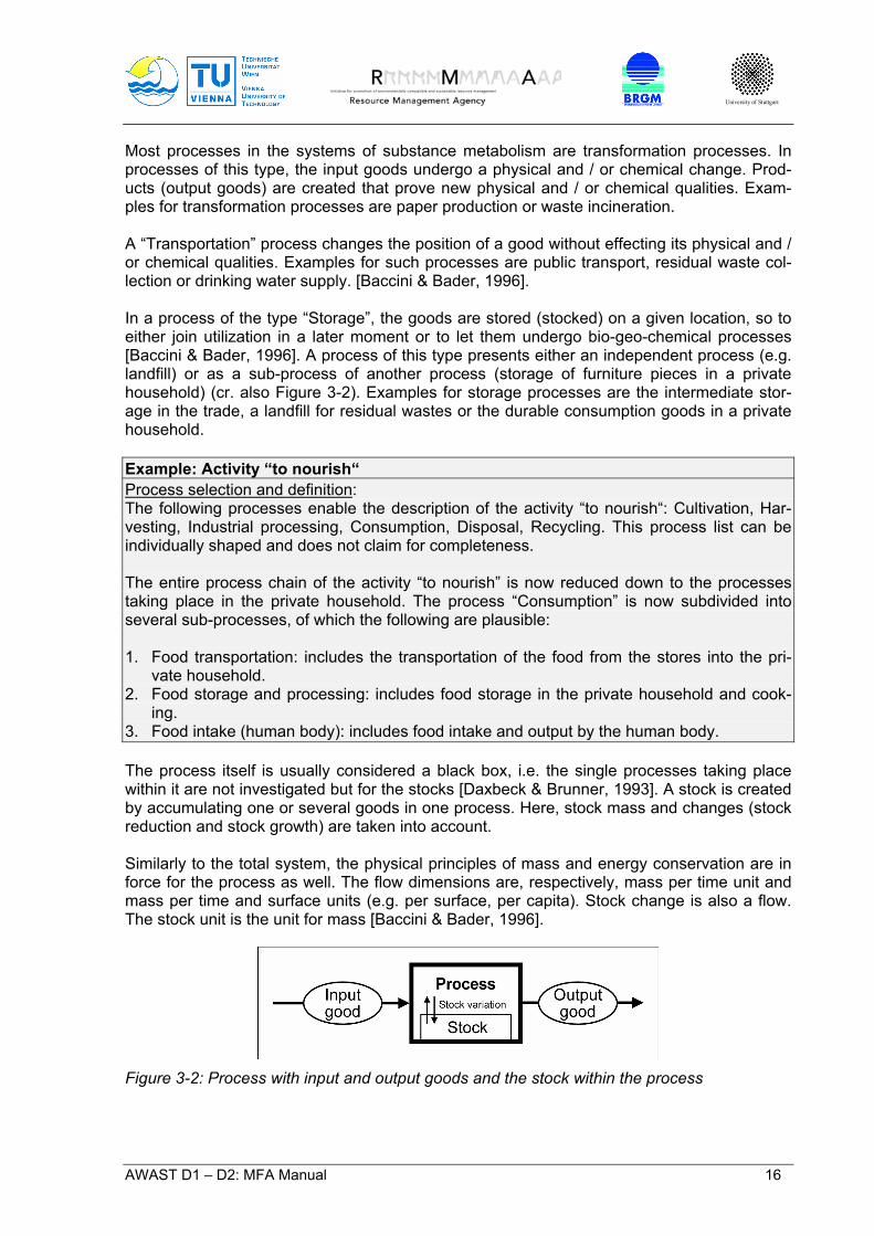
ing. 3. Food intake (human body): includes food intake and output by the human body. The process itself is usually considered a black box, i.e. the single processes taking place within it are not investigated but for the stocks [Daxbeck & Brunner, 1993]. A stock is created by accumulating one or several goods in one process. Here, stock mass and changes (stock reduction and stock growth) are taken into account. Similarly to the total system, the physical principles of mass and energy conservation are in force for the process as well. The flow dimensions are, respectively, mass per time unit and mass per time and surface units (e.g. per surface, per capita). Stock change is also a flow. The stock unit is the unit for mass [Baccini & Bader, 1996].
Figure 3-2: Process with input and output goods and the stock within the process
University of Stuttgart
AWAST D1 – D2: MFA Manual 17
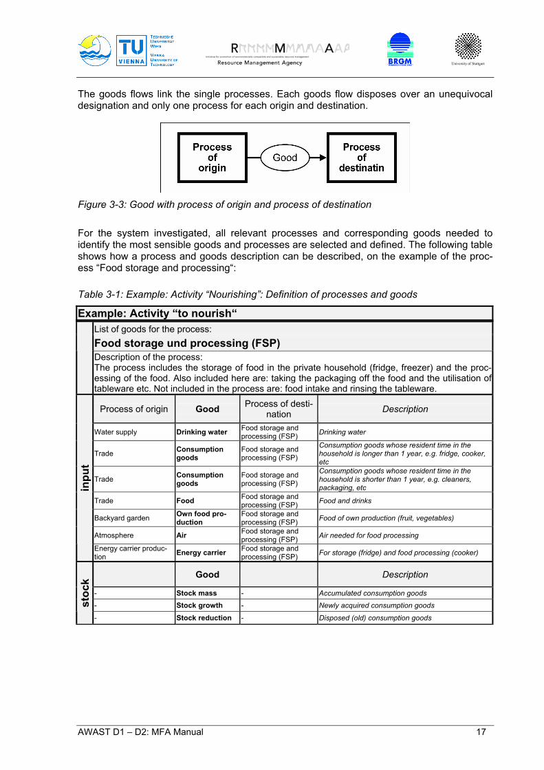
The goods flows link the single processes. Each goods flow disposes over an unequivocal designation and only one process for each origin and destination.
Figure 3-3: Good with process of origin and process of destination
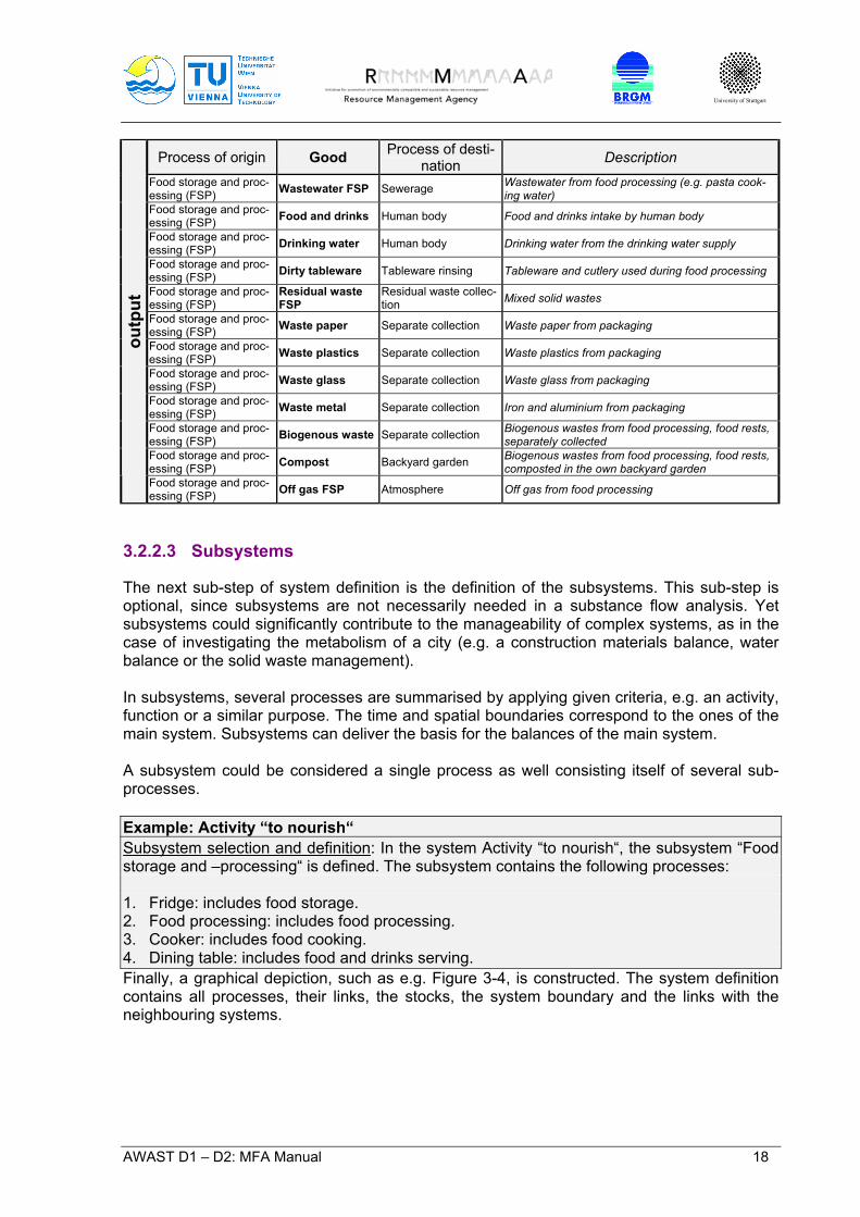
For the system investigated, all relevant processes and corresponding goods needed to identify the most sensible goods and processes are selected and defined. The following table shows how a process and goods description can be described, on the example of the proc-ess “Food storage and processing“:
Table 3-1: Example: Activity “Nourishing”: Definition of processes and goods
List of goods for the process: Food storage und processing (FSP)
Description of the process: The process includes the storage of food in the private household (fridge, freezer) and the proc-essing of the food. Also included here are: taking the packaging off the food and the utilisation of tableware etc. Not included in the process are: food intake and rinsing the tableware.
Process of origin Good Process of desti-nation Description
Water supply Drinking water Food storage and processing (FSP) Drinking water
Trade Consumption goods
Food storage and processing (FSP)
Consumption goods whose resident time in the household is longer than 1 year, e.g. fridge, cooker, etc
Trade Consumption goods
Food storage and processing (FSP)
Consumption goods whose resident time in the household is shorter than 1 year, e.g. cleaners, packaging, etc
Trade Food Food storage and processing (FSP) Food and drinks
Backyard garden Own food pro-duction
Food storage and processing (FSP) Food of own production (fruit, vegetables)
Atmosphere Air Food storage and processing (FSP) Air needed for food processing
inpu
t
Energy carrier produc-tion Energy carrier Food storage and
processing (FSP) For storage (fridge) and food processing (cooker)
Good Description
- Stock mass - Accumulated consumption goods
- Stock growth - Newly acquired consumption goods stoc
k
- Stock reduction - Disposed (old) consumption goods
Example: Activity “to nourish“
University of Stuttgart
AWAST D1 – D2: MFA Manual 18
Process of origin Good Process of desti-nation Description
Food storage and proc-essing (FSP) Wastewater FSP Sewerage Wastewater from food processing (e.g. pasta cook-
ing water) Food storage and proc-essing (FSP) Food and drinks Human body Food and drinks intake by human body
Food storage and proc-essing (FSP) Drinking water Human body Drinking water from the drinking water supply
Food storage and proc-essing (FSP) Dirty tableware Tableware rinsing Tableware and cutlery used during food processing
Food storage and proc-essing (FSP)
Residual waste FSP
Residual waste collec-tion Mixed solid wastes
Food storage and proc-essing (FSP) Waste paper Separate collection Waste paper from packaging
Food storage and proc-essing (FSP) Waste plastics Separate collection Waste plastics from packaging
Food storage and proc-essing (FSP) Waste glass Separate collection Waste glass from packaging
Food storage and proc-essing (FSP) Waste metal Separate collection Iron and aluminium from packaging
Food storage and proc-essing (FSP) Biogenous waste Separate collection Biogenous wastes from food processing, food rests,
separately collected Food storage and proc-essing (FSP) Compost Backyard garden Biogenous wastes from food processing, food rests,
composted in the own backyard garden
outp
ut
Food storage and proc-essing (FSP) Off gas FSP Atmosphere Off gas from food processing
3.2.2.3 Subsystems
The next sub-step of system definition is the definition of the subsystems. This sub-step is optional, since subsystems are not necessarily needed in a substance flow analysis. Yet subsystems could significantly contribute to the manageability of complex systems, as in the case of investigating the metabolism of a city (e.g. a construction materials balance, water balance or the solid waste management). In subsystems, several processes are summarised by applying given criteria, e.g. an activity, function or a similar purpose. The time and spatial boundaries correspond to the ones of the main system. Subsystems can deliver the basis for the balances of the main system. A subsystem could be considered a single process as well consisting itself of several sub-processes. Example: Activity “to nourish“ Subsystem selection and definition: In the system Activity “to nourish“, the subsystem “Food storage and –processing“ is defined. The subsystem contains the following processes: 1. Fridge: includes food storage. 2. Food processing: includes food processing. 3. Cooker: includes food cooking. 4. Dining table: includes food and drinks serving. Finally, a graphical depiction, such as e.g. Figure 3-4, is constructed. The system definition contains all processes, their links, the stocks, the system boundary and the links with the neighbouring systems.

University of Stuttgart
AWAST D1 – D2: MFA Manual 19
adapted fromH. Daxbeck, 1993
= flow (of goods)= good
import export
system boundary
B
C
s
x
u
t
v
w
y
z
process of originof goods t and u
Aprocess of destination
of good s
input good ofprocess A
output good ofprocess A
input good ofprocess B
output good ofprocess Bstock variation
storage
= process
import good
export good
export good
E
F
D
Figure 3-4: System definition
3.2.2.4 Selection of Substances
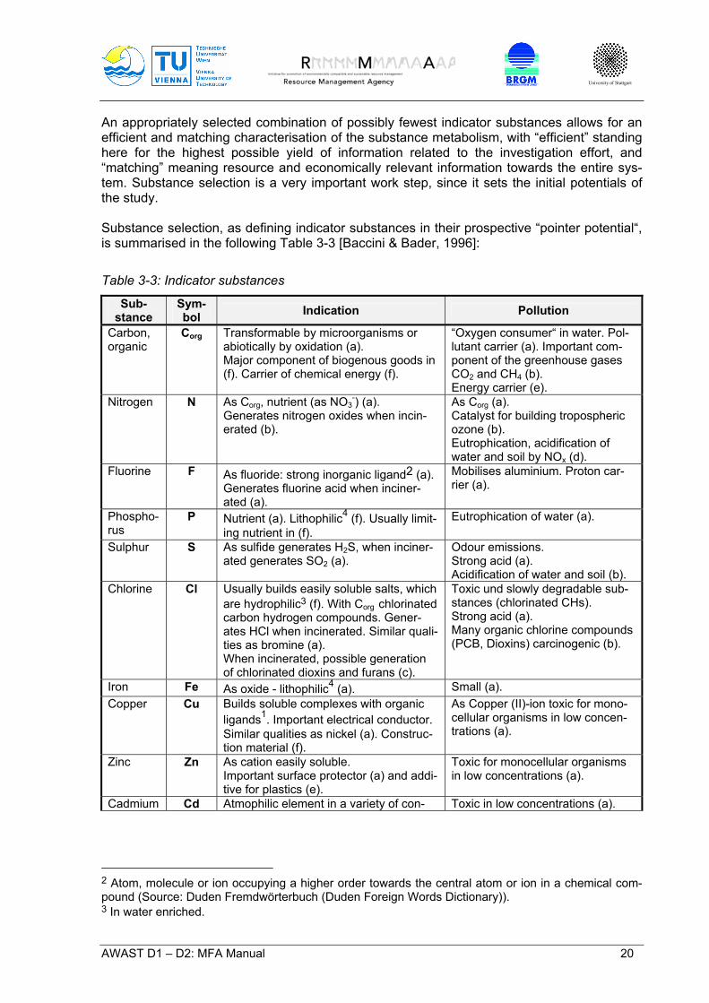
The system definition is complete when the substances have been selected. The choice of substances selection may have already been set by the study objective (e.g. depiction of the silver household of a region) or by certain legal regulations (e.g. prohibition of FCCH use) or by the potential of the particular substance as a resource (e.g. aluminium) or as a pollutant (e.g. lead). Reasons for selecting a certain substance as an indicator can be given by: 1. the substance being a significant pointer for the system in question, e.g. carbon as a major component of paper would be an indicator for the paper household of a region; 2. the chemical behaviour of the substance indicating the behaviour of another substance, e.g. nickel would behave simi-larly to copper, considering some of their chemical qualities [Baccini & Bader, 1996]. Since the number of the substances selected plays a significant role as to the funding needed, the proper selection of the substance should be paid highest attention. Table 3-2 presents some examples on indicator substances employed for purposes of con-trol, in accordance with the objectives of the EU waste management:
Table 3-2: Objectives of European waste management and adequate indicator substances
Objectives (EU waste management) Indicator Type Examples for Indicators Waste harmlessness Pollutant Lead, Cadmium, Chlorine, Chrome Resource saving Raw material Iron, Aluminium, Zinc, Copper, Nickel Recycling Raw material Iron, Aluminium, Zink, Kupfer, Nickel Recycling Energy carrier Carbon Protection of humans and environment Pollutant Lead, Cadmium, Chlorine, Chrome
University of Stuttgart
AWAST D1 – D2: MFA Manual 20
An appropriately selected combination of possibly fewest indicator substances allows for an efficient and matching characterisation of the substance metabolism, with “efficient” standing here for the highest possible yield of information related to the investigation effort, and “matching” meaning resource and economically relevant information towards the entire sys-tem. Substance selection is a very important work step, since it sets the initial potentials of the study. Substance selection, as defining indicator substances in their prospective “pointer potential“, is summarised in the following Table 3-3 [Baccini & Bader, 1996]:
Table 3-3: Indicator substances
Sub-stance
Sym-bol Indication Pollution
Carbon, organic
Corg Transformable by microorganisms or abiotically by oxidation (a). Major component of biogenous goods in (f). Carrier of chemical energy (f).
“Oxygen consumer“ in water. Pol-lutant carrier (a). Important com-ponent of the greenhouse gases CO2 and CH4 (b). Energy carrier (e).
Nitrogen N As Corg, nutrient (as NO3-) (a).
Generates nitrogen oxides when incin-erated (b).
As Corg (a). Catalyst for building tropospheric ozone (b). Eutrophication, acidification of water and soil by NOx (d).
Fluorine F As fluoride: strong inorganic ligand2 (a). Generates fluorine acid when inciner-ated (a).
Mobilises aluminium. Proton car-rier (a).
Phospho-rus
P Nutrient (a). Lithophilic4 (f). Usually limit-ing nutrient in (f).
Eutrophication of water (a).
Sulphur S As sulfide generates H2S, when inciner-ated generates SO2 (a).
Odour emissions. Strong acid (a). Acidification of water and soil (b).
Chlorine Cl Usually builds easily soluble salts, which are hydrophilic3 (f). With Corg chlorinated carbon hydrogen compounds. Gener-ates HCl when incinerated. Similar quali-ties as bromine (a). When incinerated, possible generation of chlorinated dioxins and furans (c).
Toxic und slowly degradable sub-stances (chlorinated CHs). Strong acid (a). Many organic chlorine compounds (PCB, Dioxins) carcinogenic (b).
Iron Fe As oxide - lithophilic4 (a). Small (a). Copper Cu Builds soluble complexes with organic
ligands1. Important electrical conductor. Similar qualities as nickel (a). Construc-tion material (f).
As Copper (II)-ion toxic for mono-cellular organisms in low concen-trations (a).
Zinc Zn As cation easily soluble. Important surface protector (a) and addi-tive for plastics (e).
Toxic for monocellular organisms in low concentrations (a).
Cadmium Cd Atmophilic element in a variety of con- Toxic in low concentrations (a).
2 Atom, molecule or ion occupying a higher order towards the central atom or ion in a chemical com-pound (Source: Duden Fremdwörterbuch (Duden Foreign Words Dictionary)). 3 In water enriched.
University of Stuttgart
AWAST D1 – D2: MFA Manual 21
Sub-stance
Sym-bol Indication Pollution
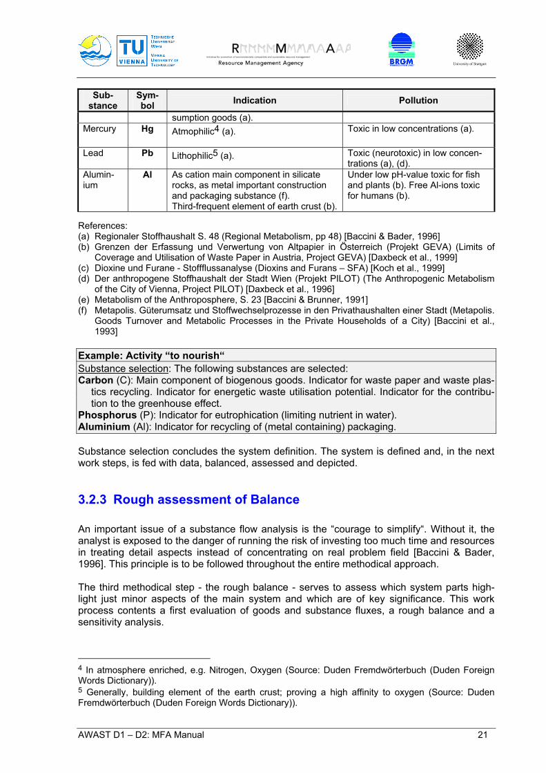
sumption goods (a). Mercury Hg Atmophilic4 (a).
Toxic in low concentrations (a).
Lead Pb Lithophilic5 (a). Toxic (neurotoxic) in low concen-trations (a), (d).
Alumin-ium
Al As cation main component in silicate rocks, as metal important construction and packaging substance (f). Third-frequent element of earth crust (b).
Under low pH-value toxic for fish and plants (b). Free Al-ions toxic for humans (b).
References: (a) Regionaler Stoffhaushalt S. 48 (Regional Metabolism, pp 48) [Baccini & Bader, 1996] (b) Grenzen der Erfassung und Verwertung von Altpapier in Österreich (Projekt GEVA) (Limits of
Coverage and Utilisation of Waste Paper in Austria, Project GEVA) [Daxbeck et al., 1999] (c) Dioxine und Furane - Stoffflussanalyse (Dioxins and Furans – SFA) [Koch et al., 1999] (d) Der anthropogene Stoffhaushalt der Stadt Wien (Projekt PILOT) (The Anthropogenic Metabolism
of the City of Vienna, Project PILOT) [Daxbeck et al., 1996] (e) Metabolism of the Anthroposphere, S. 23 [Baccini & Brunner, 1991] (f) Metapolis. Güterumsatz und Stoffwechselprozesse in den Privathaushalten einer Stadt (Metapolis.
Goods Turnover and Metabolic Processes in the Private Households of a City) [Baccini et al., 1993]
Example: Activity “to nourish“ Substance selection: The following substances are selected: Carbon (C): Main component of biogenous goods. Indicator for waste paper and waste plas-
tics recycling. Indicator for energetic waste utilisation potential. Indicator for the contribu-tion to the greenhouse effect.
Phosphorus (P): Indicator for eutrophication (limiting nutrient in water). Aluminium (Al): Indicator for recycling of (metal containing) packaging. Substance selection concludes the system definition. The system is defined and, in the next work steps, is fed with data, balanced, assessed and depicted. 3.2.3 Rough assessment of Balance
An important issue of a substance flow analysis is the “courage to simplify“. Without it, the analyst is exposed to the danger of running the risk of investing too much time and resources in treating detail aspects instead of concentrating on real problem field [Baccini & Bader, 1996]. This principle is to be followed throughout the entire methodical approach. The third methodical step - the rough balance - serves to assess which system parts high-light just minor aspects of the main system and which are of key significance. This work process contents a first evaluation of goods and substance fluxes, a rough balance and a sensitivity analysis.
4 In atmosphere enriched, e.g. Nitrogen, Oxygen (Source: Duden Fremdwörterbuch (Duden Foreign Words Dictionary)). 5 Generally, building element of the earth crust; proving a high affinity to oxygen (Source: Duden Fremdwörterbuch (Duden Foreign Words Dictionary)).
University of Stuttgart
AWAST D1 – D2: MFA Manual 22
The results of the rough balance and the sensitivity analysis are needed for:
A general understanding of the system and the role of is components (goods, proc-esses, subsystems). Goods and processes of relevance for the study objectives are identified.
Sorting out insignificant goods and processes for the further investigation. Optimising the system definition (iterative approach). For planning the work intensity for the study (data collection and description) and for
the single system components. 3.2.3.1 Rough Collecting and Processing of Data
Special emphasis is given to a rough quantitative assessment not of the numerical data but of possibly all goods, i.e. literature data are generally sufficient. The work approach includes:
Goods data collection (goods fluxes and substance concentrations). Conversion of the raw data into input and output fluxes. Calculation of the substance fluxes out of the goods fluxes and substance concentra-
tions. 3.2.3.2 Rough balancing
The balances for the goods and substance flows of the single processes in the subsystems and the main system are constructed. [Baccini & Bader, 1996]. According to the law of mass conservation, the mass balance of a process can be described by the following equation:
StockOutputInputj
ji
i ∆+= ∑∑ (Equation 3-1)
∆Stock gives the stock change within the process, whose value is positive for stock growth and negative for stock reduction. 3.2.3.3 Sensitivity analysis
In this work sub-step, the role of the single system components is investigated. The sensitivity analysis studies the effect of the parameters, respectively, of their fluctuations on the system variables. In a simple input – output model, such parameters are the import flows and the transfer coefficients (cr. Chapter 3.2.6). The system variables are all other flows in this model. It is investigated how much the system variables change when the sys-tem parameters change, and which system parameters are the most relevant (most sensi-tive) ones for a system variable or the entire system. This information is of significance for the comprehension, the steering and the optimisation of the entire system [Baccini & Bader, 1996].

University of Stuttgart
AWAST D1 – D2: MFA Manual 23
By means of sensitivity analysis the processes and goods are identified that cause the strongest reaction of the entire system. This way, the base is created for defining priorities for the following research and calculations. The sensitivity analysis is an important intermediate work step in the progress of a substance flow analysis. It enables testing the study objectives definition towards their suitability and delivers first answers. In an iterative work step, objectives and research questions (and thus the system definition as well) can be tested and adjusted within the sensitivity. 3.2.4 Planning and Performance of a Research or Measurement
Programme
In this work step, a research or measurement programme is planned based on the sensitivity analysis performed. An important issue of the planning is what dimension a good or a proc-ess should prove, so to be considerable within the further study. This mainly depends on the study objectives. Setting this limit is individual. In the studies so far done, flows < 1 % of the largest flow have proved not to be reasonable to take further into account. However, it is necessary to check the validity of this assumption for each substance and each new system. The work approach includes:
Planning the investigation or measurement programme: Setting the research pro-gramme fort he processes and their goods. Data availability and quality test for the ma-terial assessed by the rough data collection in the previous work step. If data situation proves to be insufficient, a special measurement programme is to be planned.
Data collection either by means of a literature study, questionnaires or measurements. Determination of goods flows and substance concentrations. Description of the methodical approach. Data description: here, data source and exactness declaration is of highest relevance
(Value spectrum or minimal, average and maximal values). General and technical description of the goods and processes with a view to a better
comprehensibility of the raw data. 3.2.5 Goods Fluxes Calculation
In the fifth methodical work step, the raw data for the balance of the processes, subsystems and the entire system are processed. The approach includes:
Goods flows calculation: calculation, squaring and calibration of the data. Substance flows calculation multiplication of the goods flows with the substance con-
centrations. Substance flows balance: squaring and calibration of the data.
Data squaring stands for converting the raw data into input and output flows. The dimension of the flows to balance is mass per time units, respectively mass per time and surface units (e.g. per surface, per capita). Data calibration is made by comparing the input flows with the output flows, whereas any stock change is considered. This way, flows are eventually localised that do not correspond
University of Stuttgart
AWAST D1 – D2: MFA Manual 24
to each other, i.e. the balance does not work out. If the latter should occur, the following is to do:
An analysis which flows could be wrong or not exactly enough elaborated. A repeated test of the data material, eventually, a repeated data collection. Applying a data value spectrum for single flows and testing if within this spectrum the
flows can be balanced. This approach results in a calibrated system. The accuracy aimed at for goods and sub-stance balances amounts to min. ± 20 %. 3.2.6 Transfer Function and Transfer Coefficients Calculation
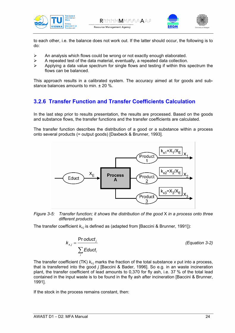
In the last step prior to results presentation, the results are processed. Based on the goods and substance flows, the transfer functions and the transfer coefficients are calculated. The transfer function describes the distribution of a good or a substance within a process onto several products (= output goods) [Daxbeck & Brunner, 1993].
Figure 3-5: Transfer function; it shows the distribution of the good X in a process onto three
different products
The transfer coefficient kx,j is defined as (adapted from [Baccini & Brunner, 1991]):
∑=
ii
jjx
Educt
oductk
Pr, (Equation 3-2)
The transfer coefficient (TK) kx,j marks the fraction of the total substance x put into a process, that is transferred into the good j [Baccini & Bader, 1996]. So e.g. in an waste incineration plant, the transfer coefficient of lead amounts to 0,370 for fly ash, i.e. 37 % of the total lead contained in the input waste is to be found in the fly ash after incineration [Baccini & Brunner, 1991]. If the stock in the process remains constant, then:
University of Stuttgart
AWAST D1 – D2: MFA Manual 25
1, =∑j
jxk (Equation 3-3)
The substance transfer coefficients are independent of the composition of total input and thus count to the system parameter. The transfer coefficient is a constant, process-defined key value being dependent on the facility and the operation mode. The goods transfer coefficients are no system parameter, since they do depend on the com-position of the input. So for instance, the goods transfer in a waste incineration facility is a function of the ash content of the input. Transfer coefficients suit:
A manageable depiction of the results. As a start basis, the assessment of substance enrichment or dilution.
3.3 Results Presentation and interpretation
Results presentation and Interpretation is performed in the following steps:
Results depiction by means of tables and graphs. Goods and substance flow diagrams, tables and graphic depictions of the transfer coefficients.
Assessment of achieving the goals and objectives of the study. 3.3.1 Tables and Graphs
For an attractive presentation, the results from goods and substance balances should be reduced once again onto the main statements and messages, whereas special attention should be paid most of all to comprehensibility [Daxbeck & Brunner, 1993]. The crucial processes, goods and substance fluxes should appear immediately recognisable, where the stress should be put on the most important statements of the project towards its objectives. Further, the limits and the uncertainties of the method selected and the data cov-erage, respectively value spectrum, should be outlined. The results are usually presented with a view to the entire system, the subsystems and even-tually, for certain processes. The results usually contain, on a goods and substance level, the following:
Tabular depiction of the average values and value spectrum for all considered flows. Graphic depictions of the average values for all flows considered by means of goods
and substances diagrams (cr. Figure 3-7). Sums of input (resp. import) flows and the output (resp. export) flows and their com-
parison; discussion and explanation of any discrepancies. Depiction of the key processes of the system or the subsystems, related to the mass
turnover on a goods or substance level. Depiction of the key goods of the system, subsystems or processes, related to the
mass or substance flow.

University of Stuttgart
AWAST D1 – D2: MFA Manual 26
Identification of the key sources and sinks of the substances considered. Identification of the theoretical possibilities for controlling, be it by changing the goods
or the process technology so to adjust to the processes or by changing the substance concentrations.
Explanation of eventual gaps and uncertainties of the data material. Here to follow, two examples for graphic depiction of the transfer coefficients, e.g. for the waste incineration plant in Wels (Austria) and an MFA of paper for Austria.
Cd
Flue Gas <0.005
Treated Ash 34+9
Cleaned WW0.04+0.03
Filter Cake 58+11
Bottom Ash 8+4
"Was
te" 1
00 %
Figure 3-6: Example for visualisation of a transfer function: Cadmium distribution in the
waste incineration plant in Wels (Austria) - Project MAPE III; ww: wastewater. [Morf et al., 1997]
Figure 3-6 shows, on the example of the substance Cadmium, its distribution onto the single output goods, based on the transfer coefficients of an incineration plant. This depiction allows for a very fast and manageable assessment of the role of each particular flow. Figure 3-7 gives an example for presenting graphically a goods balance. Clearly depicting the goods flows by applying arrows of different strength results in giving the immediate mes-sage which processes and goods are the key ones in this system. Additionally to the presen-tation of the entire system, the subsystems can be separately depicted as well in similar graphs if needed.
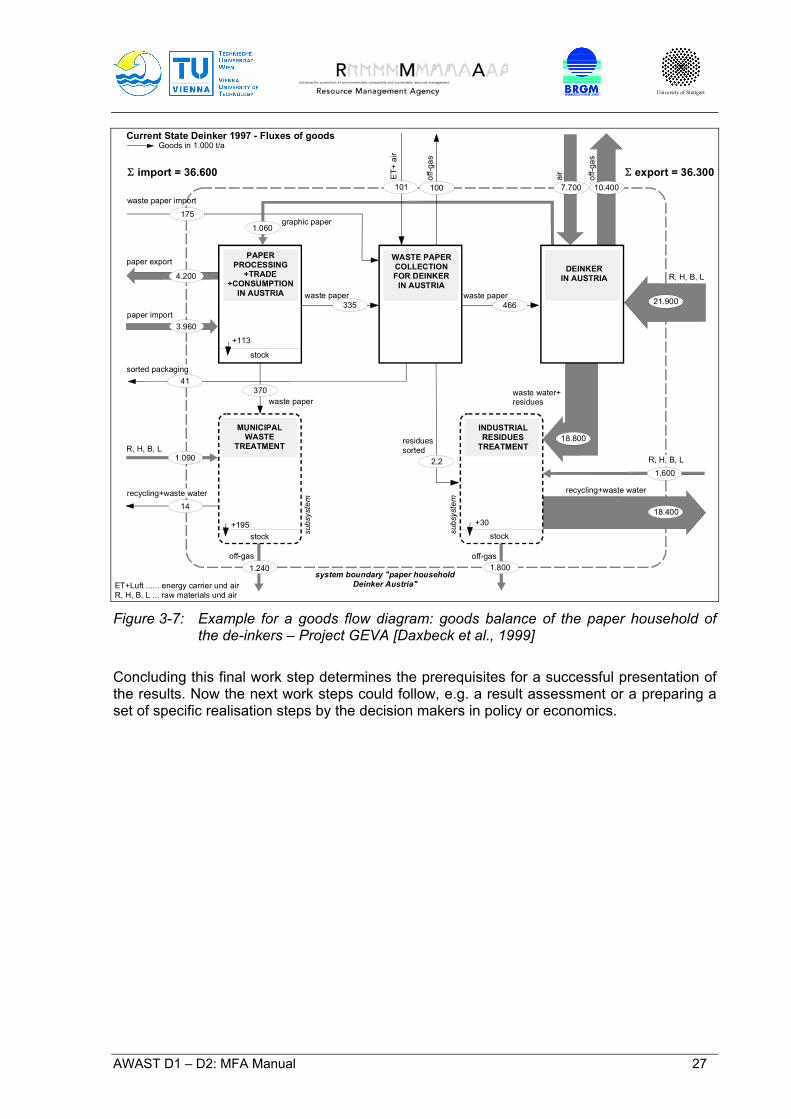
University of Stuttgart
AWAST D1 – D2: MFA Manual 27
recycling+waste water
air
R, H, B, L
R, H, B, L
waste paper import
graphic paper
residuessorted
off-gas
sorted packaging
waste water+residueswaste paper
system boundary "paper householdDeinker Austria"
paper import
paper export
ET+
air
off-g
as
off-g
as
R, H, B, L
off-gas
waste paper
recycling+waste water
subs
yste
m
subs
yste
m
PAPER PROCESSING
+TRADE+CONSUMPTION
IN AUSTRIA
WASTE PAPERCOLLECTIONFOR DEINKER
IN AUSTRIA
DEINKERIN AUSTRIA
INDUSTRIALRESIDUES
TREATMENT
MUNICIPALWASTE
TREATMENT
ET+Luft ...... energy carrier und airR, H, B, L ... raw materials und air
175
1.060
4.200
3.960
41
14
370
2,2
1.800
466 21.900
stock
stock stock
101 100 7.700 10.400
18.800
1.600
18.400
1.090
1.240
Current State Deinker 1997 - Fluxes of goods Goods in 1.000 t/a
335
Σ import = 36.600 Σ export = 36.300
+195
+113
+30
waste paper
Figure 3-7: Example for a goods flow diagram: goods balance of the paper household of
the de-inkers – Project GEVA [Daxbeck et al., 1999]
Concluding this final work step determines the prerequisites for a successful presentation of the results. Now the next work steps could follow, e.g. a result assessment or a preparing a set of specific realisation steps by the decision makers in policy or economics.

University of Stuttgart
AWAST D1 – D2: MFA Manual 28
University of Stuttgart
AWAST D1 – D2: MFA Manual 29
4 Application of MFA in Waste Management
This chapter describes the goals of the waste management. Examples are presented that illustrate the possible contribution of the MFA for achieving these goals. Further, the usability and the advantages of the MFA are demonstrated. Two important goals of waste management are the protection of human health and the envi-ronment and resource conservation. The MFA delivers quantitative and qualitative informa-tion on substances that could present a resource or a pollutant or an indicator for them. 4.1 Objectives of the Waste Management
This section deals with the legal frame of waste management systems with its objectives being paid special attention. The European Community has adopted several directives on waste management based on the following reasons:
Creation of equal conditions of competition for the common market [Directive 75/442/EEC, 1975].
Aims of the Community in the sphere of protection of the environment and improve-ment of the quality of life [Directive 75/442/EEC, 1975].
Establishment of a high level of environmental protection [Directive 91/156/EEC, 1991]. Some of the most important directives towards waste management are:
Directive on waste [Directive 75/442/EEC, 1975] Council Directive amending Directive 75/442/EEC on waste [Directive 91/156/EEC,
1991] Commission Decision of 24 May 1996 adapting Annexes IIA and IIB to Council Direc-
tive 75/442/EEC on waste [Decision 96/350/EC, 1996] Directive on packaging and packaging waste [Directive 94/62/EC, 1994] Directive on the landfill of waste [Directive 1999/31/EC, 1999] Directive on the incineration of waste [Directive 2000/76/EC, 2000]
The directives have to be implemented within a given time limit in the national regulations of the member states. The national laws, regulations and administrative provisions complying with the European directives shall contain a reference to them. The amended directive on waste (DoW) [Directive 91/156/EEC, 1991] is based on the con-sideration of the following reasons6:
Protection of human health and the environment against harmful effects caused by the collection, transport, treatment, storage and tipping of waste.
6 First two points from the introduction of the Directive on waste Directive 75/442/EEC (1975) Directive on waste., rest from the introduction of the amended directive Directive 91/156/EEC (1991) Council Directive amending Directive 75/442/EEC on waste..

University of Stuttgart
AWAST D1 – D2: MFA Manual 30
Encouragement of the material recovery of waste and of the use of recovered materials in order to conserve natural resources.
Common terminology and a definition of waste are needed in order to improve the effi-ciency of waste management in the Community.
In order to achieve a high level of environmental protection, the Member States must, in addition to taking action to ensure the responsible removal and recovery of waste, take measures to restrict the production of waste particularly by promoting clean tech-nologies and products which can be recycled and re-used, taking into consideration ex-isting or potential market opportunities for recovered waste.
Any disparity between Member States' laws on waste disposal and recovery can affect the quality of the environment and interfere which the functioning of the internal market.
It is desirable to encourage the recycling of waste and re-use of waste as raw materi-als.
It may be necessary to adopt specific rules for re-usable waste. It is important for the Community as a whole to become self-sufficient in waste disposal
and it is desirable for Member States individually to aim at such self-sufficiency. In order to achieve the above mentioned objectives, waste management plans should
be drawn up in the Member States. Movements of waste should be reduced.
Articles 3 to 5 of the amended directive on waste (DoW) [Directive 91/156/EEC, 1991] de-termine the objectives of waste management in Europe:
Article 3
1. Member States shall take appropriate measures to encourage: (a) firstly, the prevention or reduction of waste production and its harmfulness, in par-
ticular by: - the development of clean technologies more sparing in their use of natural re-
sources, - the technical development and marketing of products designed so as to make
no contribution or to make the smallest possible contribution, by the nature of their manufacture, use or final disposal, to increasing the amount or harmful-ness of waste and pollution hazards,
- the development of appropriate techniques for the final disposal of dangerous substances contained in waste destined for recovery;
(b) secondly: (i) the recovery of waste by means of recycling, re-use or reclamation or any other
process with a view to extracting secondary raw materials, or (ii) the use of waste as a source of energy.
2. Except where Council Directive 83/189/EEC of 28 March 1983 laying down a procedure for the provision of information in the field of technical standards and regulations ap-plies, Member States shall inform the Commission of any measures they intend to take to achieve the aims set out in paragraph 1. The Commission shall inform the other Member States and the committee referred to in Article 18 of such measures.
Article 4 Member States shall take the necessary measures to ensure that waste is recovered or disposed of without endangering human health and without using processes or methods which could harm the environment, and in particular: - without risk to water, air, soil and plants and animals, - without causing a nuisance through noise or odours, - without adversely affecting the countryside or places of special interest.
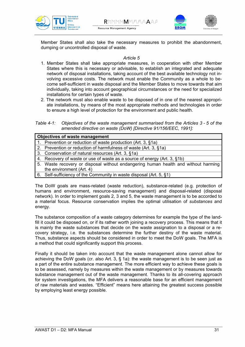
University of Stuttgart
AWAST D1 – D2: MFA Manual 31
Member States shall also take the necessary measures to prohibit the abandonment, dumping or uncontrolled disposal of waste.
Article 5 1. Member States shall take appropriate measures, in cooperation with other Member
States where this is necessary or advisable, to establish an integrated and adequate network of disposal installations, taking account of the best available technology not in-volving excessive costs. The network must enable the Community as a whole to be-come self-sufficient in waste disposal and the Member States to move towards that aim individually, taking into account geographical circumstances or the need for specialized installations for certain types of waste.
2. The network must also enable waste to be disposed of in one of the nearest appropri-ate installations, by means of the most appropriate methods and technologies in order to ensure a high level of protection for the environment and public health.
Table 4-1: Objectives of the waste management summarised from the Articles 3 - 5 of the amended directive on waste (DoW) [Directive 91/156/EEC, 1991]:
Objectives of waste management 1. Prevention or reduction of waste production (Art. 3, §1a) 2. Prevention or reduction of harmfulness of waste (Art. 3, §1a) 3. Conservation of natural resources (Art. 3, §1a) 4. Recovery of waste or use of waste as a source of energy (Art. 3, §1b) 5. Waste recovery or disposal without endangering human health and without harming
the environment (Art. 4) 6. Self-sufficiency of the Community in waste disposal (Art. 5, §1)
The DoW goals are mass-related (waste reduction), substance-related (e.g. protection of humans and environment, resource-saving management) and disposal-related (disposal network). In order to implement goals 2, 3 and 5, the waste management is to be accorded to a material focus. Resource conservation implies the optimal utilisation of substances and energy. The substance composition of a waste category determines for example the type of the land-fill it could be disposed on, or if its rather worth joining a recovery process. This means that it is mainly the waste substances that decide on the waste assignation to a disposal or a re-covery strategy, i.e. the substances determine the further destiny of the waste material. Thus, substance aspects should be considered in order to meet the DoW goals. The MFA is a method that could significantly support this process. Finally it should be taken into account that the waste management alone cannot allow for achieving the DoW goals (cr. also Art. 3, § 1a): the waste management is to be seen just as a part of the entire substance management. The more efficient way to achieve these goals is to be assessed, namely by measures within the waste management or by measures towards substance management out of the waste management. Thanks to its all-covering approach for system investigations, the MFA delivers a reasonable base for an efficient management of raw materials and wastes. “Efficient” means here attaining the greatest success possible by employing least energy possible.
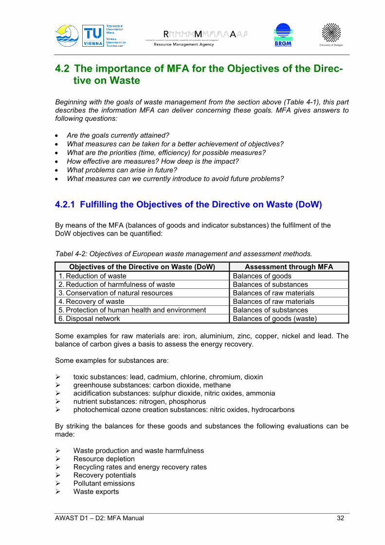
University of Stuttgart
AWAST D1 – D2: MFA Manual 32
4.2 The importance of MFA for the Objectives of the Direc-tive on Waste
Beginning with the goals of waste management from the section above (Table 4-1), this part describes the information MFA can deliver concerning these goals. MFA gives answers to following questions: • Are the goals currently attained? • What measures can be taken for a better achievement of objectives? • What are the priorities (time, efficiency) for possible measures? • How effective are measures? How deep is the impact? • What problems can arise in future? • What measures can we currently introduce to avoid future problems? 4.2.1 Fulfilling the Objectives of the Directive on Waste (DoW)
By means of the MFA (balances of goods and indicator substances) the fulfilment of the DoW objectives can be quantified:
Tabel 4-2: Objectives of European waste management and assessment methods.
Objectives of the Directive on Waste (DoW) Assessment through MFA 1. Reduction of waste Balances of goods 2. Reduction of harmfulness of waste Balances of substances 3. Conservation of natural resources Balances of raw materials 4. Recovery of waste Balances of raw materials 5. Protection of human health and environment Balances of substances 6. Disposal network Balances of goods (waste)
Some examples for raw materials are: iron, aluminium, zinc, copper, nickel and lead. The balance of carbon gives a basis to assess the energy recovery. Some examples for substances are:
toxic substances: lead, cadmium, chlorine, chromium, dioxin greenhouse substances: carbon dioxide, methane acidification substances: sulphur dioxide, nitric oxides, ammonia nutrient substances: nitrogen, phosphorus photochemical ozone creation substances: nitric oxides, hydrocarbons
By striking the balances for these goods and substances the following evaluations can be made:
Waste production and waste harmfulness Resource depletion Recycling rates and energy recovery rates Recovery potentials Pollutant emissions Waste exports
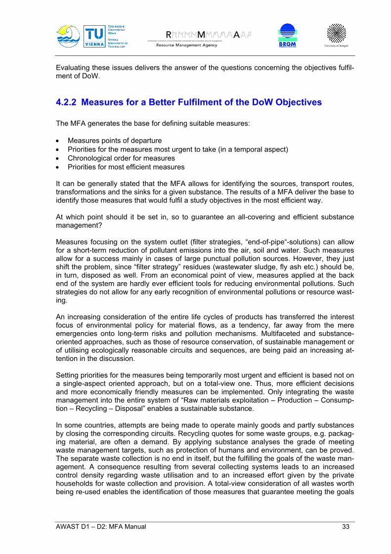
University of Stuttgart
AWAST D1 – D2: MFA Manual 33
Evaluating these issues delivers the answer of the questions concerning the objectives fulfil-ment of DoW. 4.2.2 Measures for a Better Fulfilment of the DoW Objectives
The MFA generates the base for defining suitable measures: • Measures points of departure • Priorities for the measures most urgent to take (in a temporal aspect) • Chronological order for measures • Priorities for most efficient measures It can be generally stated that the MFA allows for identifying the sources, transport routes, transformations and the sinks for a given substance. The results of a MFA deliver the base to identify those measures that would fulfil a study objectives in the most efficient way. At which point should it be set in, so to guarantee an all-covering and efficient substance management? Measures focusing on the system outlet (filter strategies, “end-of-pipe“-solutions) can allow for a short-term reduction of pollutant emissions into the air, soil and water. Such measures allow for a success mainly in cases of large punctual pollution sources. However, they just shift the problem, since “filter strategy” residues (wastewater sludge, fly ash etc.) should be, in turn, disposed as well. From an economical point of view, measures applied at the back end of the system are hardly ever efficient tools for reducing environmental pollutions. Such strategies do not allow for any early recognition of environmental pollutions or resource wast-ing. An increasing consideration of the entire life cycles of products has transferred the interest focus of environmental policy for material flows, as a tendency, far away from the mere emergencies onto long-term risks and pollution mechanisms. Multifaceted and substance-oriented approaches, such as those of resource conservation, of sustainable management or of utilising ecologically reasonable circuits and sequences, are being paid an increasing at-tention in the discussion. Setting priorities for the measures being temporarily most urgent and efficient is based not on a single-aspect oriented approach, but on a total-view one. Thus, more efficient decisions and more economically friendly measures can be implemented. Only integrating the waste management into the entire system of “Raw materials exploitation – Production – Consump-tion – Recycling – Disposal” enables a sustainable substance. In some countries, attempts are being made to operate mainly goods and partly substances by closing the corresponding circuits. Recycling quotes for some waste groups, e.g. packag-ing material, are often a demand. By applying substance analyses the grade of meeting waste management targets, such as protection of humans and environment, can be proved. The separate waste collection is no end in itself, but the fulfilling the goals of the waste man-agement. A consequence resulting from several collecting systems leads to an increased control density regarding waste utilisation and to an increased effort given by the private households for waste collection and provision. A total-view consideration of all wastes worth being re-used enables the identification of those measures that guarantee meeting the goals
University of Stuttgart
AWAST D1 – D2: MFA Manual 34
of DoW by employing the lowest effort and costs. The success of the measures is given by their contribution to fulfilling the DoW objectives. An appropriate example is given by the CFC’s: although their use was prohibited years ago, significant amounts of those are still incorporated as a stock in the infrastructure net [Obernosterer, 1994]. By registering the most relevant substance fluxes and stocks within a region, the application fields can be compared to each other. By qualifying and quantifying the products still present in the stocks, the CFC containing fluxes of wastes to expect in the future can be calculated. Priority setting towards the waste fluxes to present the greatest problem was assessed by comparing the single CFC potentials of each application field. Thus, the control and steering interfaces in the entire system could be located where the highest effect can be achieved by employing the lowest effort and costs. 4.2.3 Efficiency of Measures
A characteristic of the material flow analyses within the waste management is a similarity with regard to a phenomenon result of many studies. Often, measures taken at visible or evi-dent problem interfaces (considering in the whole system) prove to hardly be of any effi-ciency. Examples here are measures in the waste management sector, in particular in the CFC’s disposal, plastics and the licensed aluminium packaging. On the contrary, efficiency control of the measures at the scale of the entire substance metabolism would prevent from achieving a relatively low effect on the costs of a relatively high effort. The MFA allows for testing the effect of given measures and thus, for controlling the success of regulations in the sectors of waste management and environmental policy. On the one hand, the prospective state of the system can bet his way “simulated“ when certain meas-ures or a measure package would be introduced. A variety of measures can be compared to each other this way, and a choice is given for selecting the optimal one with regard to the DoW objectives. On the other hand, after a measure has already been introduced, the MFA appears a suit-able tool for examining the “correctness“ of this decision. Substance flows and transfer coef-ficients modelled in advance can be compared to the corresponding values from real meas-urements. This evaluation results in a two-fold effect: the correctness of the assumptions made can be checked, and eventually, new research questions can be generated. 4.2.4 Forecasting
The MFA is a suitable instrument to early identify the endangering of the DoW objectives, mainly in the fields of human and environment protection as well as resource saving. In par-ticular, such endangering types are:
Pollutant enrichment in the environment and the anthroposphere Emissions increase Pollutant transfers through recycling products, etc. Resource accumulation, respectively, consumption to the point of exhaustion, in
stocks.
University of Stuttgart
AWAST D1 – D2: MFA Manual 35
By applying the substance flow analysis it becomes possible to simulate future development scenarios. For example, this way substances can be identified being currently contained in stock bodies and considered to be soon disposed. The type and amount of the substance to undergo disposal can be calculated in advance, so that corresponding measures can be planned in time that secure an organised disposal accorded to the DoW objectives. The CFC’s study cited [Obernosterer, 1994] could demonstrate that methods concerned primarily with a direct waste analysis are able to recognise CFC containing wastes just when the latter have already entered the waste management sector. This means that isolated measure-ments are not capable to localise future problems. In the CFC study, the SFA was applied as an early recognition tool, whereas the CFC amounts (stocks) currently “hidden“ and accumu-lated in consumption and the potential CFC fluxes resulting from these stocks could be as-sessed. This study could show as well what amounts of CFC containing wastes come up in the future. 4.2.5 Monitoring
The key objective of the waste management is to react. Thus, the waste management is al-ways a step behind the real waste flows. The law does not explicitly foresees the issues of “Forecast” and “Monitoring of measures taken“. The legislator should issue the offer to the waste management to step over its classic field of activity, i.e. to understand and to keep the overview over the entire anthropogenic substance metabolism. This way, the waste man-agement would be given the opportunity to recognise future developments and trends in time, and would thus gain the chance to counteract and finally, to fulfil the DoW objectives more efficiently (more cost-effectively and faster). The MFA is a tool enabling a monitoring. In a variety of studies it could prove, for instance, that waste incineration plants are suitable for controlling the success of waste management measures through a continuous and cost-saving monitoring of the waste composition. 4.3 Capacity of MFA towards Waste Management
This section describes potentials of MFA for waste management. The results of MFA, bal-ances of goods, energy and substances are used as: • Direct information for elaborating recommendations, measures and conclusions • Basis for specific assessments • Basis for materials accounting and materials management A further capability of MFA within the waste management, the indirect determination of waste composition, is described in Chapter 5. The MFA is as a rule presented in flow diagrams and shows the metabolism of goods, en-ergy and substances within a defined system. The balances include detailed information (see Table 4-3) regarding the management of goods and substances.
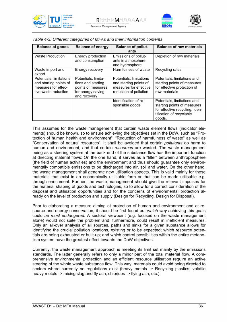
University of Stuttgart
AWAST D1 – D2: MFA Manual 36
Table 4-3: Different categories of MFAs and their information contents
Balance of goods Balance of energy Balance of pollut-ants
Balance of raw materials
Waste Production Energy production and consumption
Emissions of pollut-ants in atmosphere and hydrosphere
Depletion of raw materials
Waste import and export
Energy recovery Harmfulness of waste Recycling rates
Potentials, limitations and starting points of measures for effec-tive waste reduction
Potentials, limita-tions and starting points of measures for energy saving and recovery
Potentials, limitations and starting points of measures for effective reduction of pollution
Potentials, limitations and starting points of measures for effective protection of raw materials
Identification of re-sponsible goods
Potentials, limitations and starting points of measures for effective recycling. Iden-tification of recyclable goods.
This assumes for the waste management that certain waste element flows (indicator ele-ments) should be known, so to ensure achieving the objectives set in the DoW, such as “Pro-tection of human health and environment“, “Reduction of harmfulness of waste“ as well as “Conservation of natural resources“. It shall be avoided that certain pollutants do harm to human and environment, and that certain resources are wasted. The waste management being as a steering system at the back end of the substance flow has the important function at directing material flows: On the one hand, it serves as a “filter“ between anthroposphere (the field of human activities) and the environment and thus should guarantee only environ-mentally compatible emissions to be discharged into air, soil and water. On the other hand, the waste management shall generate new utilisation aspects. This is valid mainly for those materials that exist in an economically utilisable form or that can be made utilisable e.g. through enrichment. Further, the waste management should give the relevant impulses for the material shaping of goods and technologies, so to allow for a correct consideration of the disposal and utilisation opportunities and for the concerns of environmental protection al-ready on the level of production and supply (Design for Recycling, Design for Disposal). Prior to elaborating a measure aiming at protection of human and environment and at re-source and energy conservation, it should be first found out which way achieving this goals could be most endangered. A sectoral viewpoint (e.g. focused on the waste management alone) would not suite the problem and, furthermore, could result in inefficient measures. Only an all-over analysis of all sources, paths and sinks for a given substance allows for identifying the crucial pollution locations, existing or to be expected; which resource poten-tials are being exhausted or built-up; and which control possibilities within the entire metabo-lism system have the greatest effect towards the DoW objectives. Currently, the waste management approach is meeting its limit set mainly by the emissions standards. The latter generally refers to only a minor part of the total material flow. A com-prehensive environmental protection and an efficient resource utilisation require an active steering of the whole waste substance flow. This way, materials could avoid being directed to sectors where currently no regulations exist (heavy metals -> Recycling plastics; volatile heavy metals -> mixing slag and fly ash; chlorides -> flying ash, etc.).
University of Stuttgart
AWAST D1 – D2: MFA Manual 37
The systematic, multi-aspect design of e.g. national waste management plans towards mate-rial criteria allows for a waste management optimised towards technical, economical and ecological characteristics. 4.4 Assessment of Material Balances
The basis for all MFA assessments are balances of goods and substances. The result of the assessment is, as a rule, a physical value that can be compared with the results from alternative scenarios, respectively it registers the positive or negative changes they would cause. This value can be based on different data bases and may consider most different criteria as well (e.g. economical, ecological, social). The selection of an evaluation criterion expresses thus a certain value prioritisation as well. In the recent years, a variety of evaluation tools was developed that are based on the material flow analysis. The common goal of all these instruments is to allow for generating a summarising judgement out of the plentiful of information delivered by analysing material flows. Six evaluation methods are described in more detail below, as examples: 4.4.1 Limit Values
A simple assessment of material balances can be achieved by comparing the results with the existing legislative limit values usually available for gaseous and liquid emissions, and gen-erally concern a human-toxicological, respectively eco-toxicological background. Remaining below the limit values through purification facilities is though related to substance concentra-tion e.g. in the off-gas or the wastewater. Solid residues and emissions cannot be, on the contrary, sufficiently assessed only by sub-stance concentrations, since e.g. exceeding a limit value could be avoided through dilution with other materials. Therefore, it is necessary to consider the substance freights towards both emissions and solid residues. An example for a freight-related approach is the following one referred to below as a “geogenic-to-anthropogenic reference approach“. 4.4.2 Comparing geogenic to anthropogenic flows and stocks
In this evaluation approach, the anthropogenic flows and stocks are confronted with the cor-responding geogenic ones. This reference method takes into account the following require-ments towards a sustainable development [Sustain, 1994]. (1) Material flows induced by human activities shall not change the magnitude of the global
buffer capacity in environmental substance cycles. (2) Anthropogenic material flows shall not exceed the local assimilation capability, nor shall
they exceed the variation range of geogenic flows. According to the geogenic – anthropogenic reference approach, the effect of material flows induce by the humans on the environment is considered a key indicator. For example, changes in the process “Soil” can be investigated over the emissions of a waste incineration plant, where the current pollutant concentration in the soil, resulting from human activity is

University of Stuttgart
AWAST D1 – D2: MFA Manual 38
compared to the initial (geogenic) one existing prior to the begin of industrial processes at the given location. According to the requirements defined above, material flows can be qualified as environmen-tally compatible with regard to a sustainable development just when the geogenic flows and reservoirs would not be changed by this in a long-term perspective. Changes < 1-10 % are generally assumed to be acceptable. The exact procentual value is most often not technically justifiable but reflects a certain value prioritisation, e.g. the demand for safety of a given soci-ety (the precaution principle). 4.4.3 Critical Volume
The prerequisite needed for applying this evaluation method is the data of emitted substance and the availability of a limit value relevant for the effect of the investigated pollutant (e.g. immission limit value, maximal workplace concentration (MWPC) value, etc.), proving that below this limit, no endangering of human health, environment or infrastructure would be expected.
j
jiji GW
EV ,
, = (Equation 4-1)
where i a facility, a process or a system j a pollutant emitted into the air, soil or water Vi,j critical volume for the pollutant j for the facility, process, system i Ei,j emitted amount of the pollutant j by the facility, process, system i GWj suitable limit value for the pollutant j The critical volume Vi,j is a measure for the pollution grade of the environmental medium (air, soil, water) in question by the emission of the pollutant j, so that the limit concentration for the pollutant j is exceeded. The critical volume Vi,j links emission and immission and thus en-ables a comparison among different technologies, facilities or processes. This approach allows for relating different pollutants and for aggregating their critical single volumes to a critical total volume (for the environmental compartments air, soil and water). Critical volumes are very suitable when comparing scenarios based on material flow analy-ses.
(Equation 4-2) ∑=
=n
ijii VV
1,
where Vi critical volume for a given facility, technology, process or system by considering all
pollutants j=1...n over this technology. Vi shows the load resulting from all pollut-ants emitted by applying this technology.
University of Stuttgart
AWAST D1 – D2: MFA Manual 39
4.4.4 Substance Concentration Efficiency (SCE)
Every biological or technical system (human, waste treatment) is able to either dilute or en-rich by the majority. “Majority” stands here for the following: as a rule, a system produces many different output goods (e.g. products, wastes, emissions), and these prove very differ-ent element concentrations each. So, for example, the cadmium imported a waste incinera-tion plant through residual wastes is diluted by the purified off-gas of and enriched in the fly ash. The crucial question is if a waste incineration plant as a system presents generally the diluting or the enrichment process for cadmium. The requirement of enrichment for inorganic substances (or pollutants) is strictly stated among the goals of the Waste Management Act: to secure protection of humans and envi-ronment, emissions from the waste management are allowed to only marginally pollute the atmosphere and hydrosphere. Thus, pollutants that cannot be decomposed (e.g. heavy met-als) shall be transferred into the solid residues put out by waste management technologies. These residues can be either landfilled or utilised as resources. After-care-free disposal of residues demands either their composition to be similar to the one of earth crust or their re-peated enrichment (aiming at reducing the residual mass) followed by an immobilisation treatment and final disposal in special landfills. Utilisation of residues as a resource requires either lowering the pollutant concentration (e.g. utilisation as construction materials) or, again, achieving a very high grade of its enrichment (e.g. utilisation in the metallurgic sector). An approach for quantification of the dilution / enrichment capacity of a given technology is the method of substance concentration efficiency (SCE) [Rechberger, 1999]. The evaluation is based on the statistical entropy that quantifies distribution scattering. Several SCE values characteristic for a given element can be weighed in relation to the geogenic concentrations in air, soil and water etc and finally, be aggregated into the total evaluation value SCEtot. This approach is suitable not only for comparison of different technologies but also for optimising and managing of new technologies. So far, the approach has been tested on technologies (mechanical-biological waste treatment, waste incineration, cement production) and on sys-tems (Management of combustible wastes in Austria, Waste management of Vienna). 4.4.5 Material Input per Service Unit (MIPS)
The assessment method “Material input per Service unit“ MIPS [Schmidt-Bleek & Klüting, 1993], [Schmidt-Bleek & Behrensmeier, 1998] delivers a measure for the aggregated mass flow of goods, that arises within a service unit (e.g. hair cutting, transport). If the service unit is defined, all needed materials (input goods) and their measures are calculated. Here, the entire life cycle of the evaluation object should be registered. This material balance divides input into five categories: abiotic and biotic resources, soil, water and air. The “ecological rucksack” of each material is additionally considered, i.e. the energy and material invest-ments are taken into account as well for production, processing, transportation for both the product and the infrastructure needed for these steps. The MIPS concept defines the ap-proach for data collecting concerning the input goods, how and where to draw the system boundaries and how to deal with an insufficient data background. Regarding the application of this method onto objectives of waste management studies, the first question to be given an answer is how to define here an appropriate service unit. The latter could be interpreted as e.g. the disposal of one ton of residual waste However, since the MIPS concept is limited within the goods level, it appears suitable just for rough estimat-
University of Stuttgart
AWAST D1 – D2: MFA Manual 40
ing the effort of each disposal variant (e.g. fuel for the waste collection, supporting materials for given waste treatment technologies), as only the input of goods can be evaluated, but neither the output nor the substances contained. Thus, the MIPS method is not appropriate for evaluation of balances of goods in the waste management. Considering the concept and the current structure of the method, the latter is not yet suitable for assessing substance bal-ances, either. 4.4.6 Life Cycle Assessment (LCA)
Life Cycle Assessment (LCA), or Eco Balances, are originally methods for determining the effects of products on the environment. A LCA consists, according to the standard [ÖN EN ISO 14040, 1997], of a balance target, an object balance, an effect balance (classification and characterisation), and a balance evaluation. The object balance consists of an energy and a mass balance, inclusively the most signifi-cant emissions into air and water as well as waste amounts resulting, and the surface con-sumption. The effect balance consists of two work steps, classification and characterisation, where in the first, the results of the object balance are classified according to given “envi-ronmental effect categories” (e.g. resource demand, greenhouse effect, ozone depletion, human and ecological toxicity, etc), and the characterisation assumes the calculation of each effect category. In the balance evaluation, the results from the object and effect balances are resumed according to a given goal allowing for deriving the recommendations and conclu-sions required. Optionally, each category can be weighed and aggregated with others into a final evaluation value. However in the practice, the latter option has not proved to be of sig-nificant suitability due to the different weighing tools existing and the subjective effect on their selection. When combining MFA and LCA, single categories of environmental effects are selected fort he assessment. MFA can be applied directly or as an initial base for the LCA object balance. If the MFA should be complemented or not, depends on the requirements of the selected categories of environmental effects. 4.5 Materials Accounting
Material flow analysis requires as a rule a great effort. An elegant and cost-effective possibil-ity for the periodic update of relevant material flows is offered by the method materials ac-counting. By means of fewer and carefully selected goods or substance flows measurable within an acceptable funding, the entire flow of a given substance can be traced. Knowledge of the key processes allowing for forecasts towards the whole substance flow is a basic pre-requisite for proving the capacity of the materials. Moreover, if a material flow analysis has once been performed for a given system, a permanent update can be easily introduced [Brunner et al., 1994]. Materials accounting is used as a complementing tool to the monitoring methods existing and supplies with the base for the substance management7. Substance management means to
7 Substance management encloses all measures that could influence the manner and the range of provision with goods and substances, their utilisation in the anthroposphere and their treatment and disposal as wastes.
University of Stuttgart
AWAST D1 – D2: MFA Manual 41
discover and use potentials, to identify, reduce, substitute or avoid pollutants. The substance management does directly influence the shape and the production of goods, and thus an indirect effect on their disposal and life duration.

University of Stuttgart
AWAST D1 – D2: MFA Manual 42
University of Stuttgart
AWAST D1 – D2: MFA Manual 43
5 Determination of the composition of municipal solid waste
5.1 Introduction
5.1.1 Definition of Municipal Solid Waste
Mixed municipal solid waste means, according to the European directive on waste incinera-tion [Directive 2000/76/EC, 2000], waste from households as well as commercial, industrial and institutional waste, which because of its nature and composition is similar to waste from households, but excluding fractions indicated in the Annex to Decision 94/3/EC(22) under heading 20 01 that are collected separately at the source of origin (e.g. paper, glass, plastic, metal) and excluding other wastes indicated under heading 20 02 of that Annex (e.g. park and garden waste). 5.1.2 Objectives of Waste Analysis
The successful management of municipal solid waste depends on the knowledge of its com-position. This knowledge is necessary for municipal and industrial stakeholders involved in urban waste management to develop strategies and concepts for a sustainable municipal solid waste management, reuse and disposal. Decisions on recycling, optimisation of waste treatment processes and predictions of emissions from waste treatment require information about the content of materials and substances in municipal solid waste. Hence, the determination of the waste composition is the main objective of waste analyses. This could be either the composition in terms of fractions or the chemical and physical com-position in terms of calorific values, water contents, substance concentrations and other pa-rameters. Furthermore, the waste generation rate and the contribution of each individual waste fraction to the total composition of municipal solid waste are of interest. 5.2 Approach
5.2.1 The Life Cycle of a Good
The waste composition can be determined by focusing on different points during the life cycle of the goods generating the waste. These certain points are shown in Figure 5-1. The conventional way to determine the waste composition is done by analysing the waste itself. This so called direct waste analysis is done by a manual separation of the waste into several given fractions. Since a significant part of the waste cannot be analysed in a direct analysis, because of its small particle size, alternative methods for the determination of the waste composition were developed. These so called indirect waste analysis methods have a totally different ap-proach.
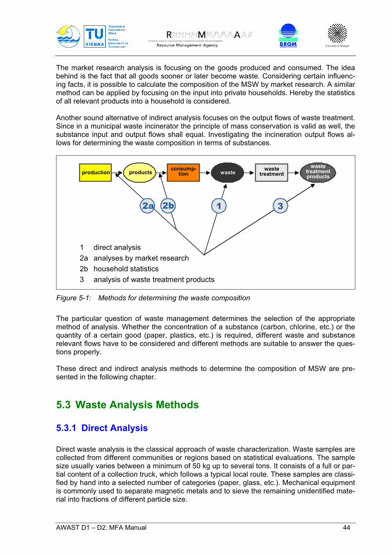
University of Stuttgart
AWAST D1 – D2: MFA Manual 44
The market research analysis is focusing on the goods produced and consumed. The idea behind is the fact that all goods sooner or later become waste. Considering certain influenc-ing facts, it is possible to calculate the composition of the MSW by market research. A similar method can be applied by focusing on the input into private households. Hereby the statistics of all relevant products into a household is considered. Another sound alternative of indirect analysis focuses on the output flows of waste treatment. Since in a municipal waste incinerator the principle of mass conservation is valid as well, the substance input and output flows shall equal. Investigating the incineration output flows al-lows for determining the waste composition in terms of substances.
2a 2b 1 3
productionconsump-
tion waste wastetreatment
wastetreatmentproducts
direct analysisanalyses by market researchhousehold statisticsanalysis of waste treatment products
12a2b3
products
Figure 5-1: Methods for determining the waste composition
The particular question of waste management determines the selection of the appropriate method of analysis. Whether the concentration of a substance (carbon, chlorine, etc.) or the quantity of a certain good (paper, plastics, etc.) is required, different waste and substance relevant flows have to be considered and different methods are suitable to answer the ques-tions properly. These direct and indirect analysis methods to determine the composition of MSW are pre-sented in the following chapter. 5.3 Waste Analysis Methods
5.3.1 Direct Analysis
Direct waste analysis is the classical approach of waste characterization. Waste samples are collected from different communities or regions based on statistical evaluations. The sample size usually varies between a minimum of 50 kg up to several tons. It consists of a full or par-tial content of a collection truck, which follows a typical local route. These samples are classi-fied by hand into a selected number of categories (paper, glass, etc.). Mechanical equipment is commonly used to separate magnetic metals and to sieve the remaining unidentified mate-rial into fractions of different particle size.
University of Stuttgart
AWAST D1 – D2: MFA Manual 45
In order to determine the chemical and physical parameters of each fraction, representative samples are drawn from each material. These samples are farther prepared (dried, pulver-ized and sieved) for laboratory analysis. The description of the methodology used to determine the composition of MSW in France is based on MODECOM, developed by ADEME (the French National Agency for Environment and Energy Management), TIRU SA (Traitement Industriel des Résidus Urbains), BRGM (the Bureau of Geological and Mining Research) and CEMAGREF (National Centre for Agricul-tural Machinery, Civil Engineering, Water and Forestry). [ADEME, 1993], [ADEME, 1997] In Austria the method of the civil engineering office Hauer [Hauer, 1999] was used for a recent waste analysis. It is based on Vogel, who has developed the methodology already in the Seventies. This method was used continuously developed in several waste analyses within the last 25 years. Furthermore a study of Lucas [Koca & Nilsson-Djerf, 2000] was used to describe both methodologies. 5.3.1.1 Description of the method used in France
5.3.1.1.1 Sampling methodology
The sampling methodology used by ADEME [ADEME, 1993], [ADEME, 1997] to support the local authorities in the assessment of their MSW and the performance of their selective col-lections, is called MODECOM. It is a flexible methodology designed to determine the compo-sition of the household waste generated by the communities on a local or regional level. The method consists of five major operations:
Preliminary inquiry, designed to collect all the data required to organize an analytical survey
Selection of collection vehicles to be sampled Constitution of samples to be sorted Sorting of samples broken down into two phases First phase: sorting of coarse elements Second phase: partial sorting of medium-size elements Laboratory analysis
The methodology starts with the collection of the data necessary to organize the waste sur-veys. Required information is as follows: 1. General characteristics of the survey area: The survey area is attempted to be described as thoroughly as possible whether it is a rural or urban municipality, a metropolitan area or an inter-municipal association. To accomplish this, the MODECOM methodology defines a procedure as given below: • Selection of all municipalities in the survey area; • Evaluation of the sedentary population (based on INSEE data municipalities are classi-
fied as rural or urban); • Identification of the nature of habitat according to type of housing (INSEE defines the
characteristics of housing according to the number of rooms or the number of flats in a building);
University of Stuttgart
AWAST D1 – D2: MFA Manual 46
• Determination of the economic activities in the survey area (based on the MAIN ACTIVITY NAP 15 nomenclature);
• Identification of any special events in the survey area which may have an influence on the nature of the waste e.g. daily or weekly open markets, local events (i.e. street sales, second hand markets etc.), seasonal activities (tourists etc.).
2. Determination of different waste flows generated in the towns of the survey area: All municipal waste flows (i.e. papers, textiles, plastic bottles, domestic waste etc.) are identi-fied and a “flow code” is given to each of them, based on a code chart developed for MODECOM. The treatment plants in the survey area are identified and the size of the collec-tion zone for each flow is then determined with reference to the actual collection routes. Fi-nally, the monthly and yearly generations of the waste flows are quantified. 3. Organization of waste collection: To be able to organize the waste collection into routes with different pick-up days and fre-quency, information regarding the days of reception of collection vehicles at the concerned treatment plant is determined. The quantities collected on each one of these days, is deter-mined as well. Any separate collections (glass, paper, scrap metal, etc.) together with their respective quantities are recorded as well. 4. Evaluation of the seasonal character: Some communities experience a medium to high seasonal activity. This is reflected by a sig-nificant change in the quantity of waste produced. In such cases, it is important to delimit the average waste amounts for the high season, as compared with the low season. The seasonality criterion is essential for the identification of non-occasional periods of high activity (at least one month). Evaluation and calculation of this seasonal character is based on the monthly waste production figures for the entire survey area and for a single reference year:
Delete the lowest month Compute the monthly mean over the six lowest remaining months Calculate for each month the ratio between the concerned month over the mean of
the six lowest months If the ratio is greater than 1.5, then the area may be regarded as having a seasonal
activity Once the necessary information to structure the organization of the waste survey is gathered, preparations for the waste sampling start. The concerned area can be either considered as a unit (i.e. a single sector) or subdivided into different sectors. Among others, some of the criterions that could be considered in the categorization of the sectors are described by the MODECOM methodology as:
The type of separate collection; The type of habitat, collective and/or housing estates (based on INSEE data); Association of municipalities according to size (rural sector, semi-urban sector, ur-
ban sector); The seasonal changes in the survey zone etc.
For all of the subdivided geographical sectors, data such as population breakdown per type of INSEE habitat, workforce breakdown per INSEE economic activity and types of collected
University of Stuttgart
AWAST D1 – D2: MFA Manual 47
flows are identified. For each flow monthly and yearly tonnages collected in a reference year, frequency of collections, type of container and type of collection are classified. After the separation of the survey area into different sectors, sampling periods are chosen. To get more accurate results, multiple surveys are conducted in different time periods (i.e. in spring, summer, autumn, winter). If the survey area includes seasonal periods (of at least one month), a minimum of one survey during one of these periods is planned. If there are no seasonal periods, surveys are chosen from any period of the year, except for atypical or ex-ceptional periods (holidays, fairs, festivals etc.) Statistical calculations performed by ADEME have shown that the precision of the waste sur-vey results depends on the number of samples analyzed and the heterogeneousness of the waste, rather than on the quantity of waste generated in the survey area. Therefore, at least five samples per survey are taken (even for the smallest survey areas) in order to determine the average composition of domestic waste in a survey area. If the survey area has a popula-tion of more than 200 000, it is preferable to increase the sample number at least to ten. If the survey area is divided into sectors, the number of samples for each sector is estimated to be at least one (proportional to waste generation in each sector). So the total number of samples collected from entire survey area is equal or greater than five. 5.3.1.1.2 Sorting and Analyzing of the Waste Samples
To collect the samples, five or more of the waste trucks transferring the waste (collected over a week) to the treatment plant are randomly selected. The selected truck empties its contents on a clean and sheltered area. With the help of a small power shovel, the waste is then col-lected into 10 containers randomly, each weighing approximately 50 kg. At the end, a waste sample of approximately 500 kg is formed for subsequent sorting and analyzing processes. Sorting nomenclature of the 15 basic categories plus sub-categories: FP – Small Fines
• < 8 mm round mesh fines FG – Large Fines
• 8-20 mm round mesh fines 1 – Fermentable Waste
• Food Waste • Yard and garden rubbish
2 – Papers
• Packaging • Newspaper-brochures • Magazines & ads on glossy paper • Other papers
3 – Cardboards
• Flat packaging cardboard • Corrugated packaging cardboard • Other cardboards

University of Stuttgart
AWAST D1 – D2: MFA Manual 48
4 – Composites • Packaging • Other composites
5 – Textiles
• Packaging • Other textiles
6 – Health Care Textiles
• Packaging • Other health care textiles
7 – Plastics
• Polyolefin films (PE & PP) • Clear PVC bottles • Clear PET bottles • Polyolefin jars & bottles • Opaque PVC jars & bottles • Opaque PET jars & bottles • Polystyrene foam packaging (PS) • Other plastic packaging • Other plastic waste
8 – Unclassified Combustibles
• Packaging • Other unclassified combustibles
9 – Glass
• Green glass packaging • Clear glass packaging • Brown glass packaging • Packaging glass other colours • Other glass waste
10 – Metals
• Ferrous metal packaging • Other ferrous metal waste • Aluminium packaging • Other aluminium waste • Other metal packaging • Other metal waste
11 – Unclassified Incombustibles
• Unclassified incombustible packaging • Other unclassified incombustibles
12 – Special waste
• Alkaline batteries • Saline batteries • Rechargeable batteries • Button power cells
University of Stuttgart
AWAST D1 – D2: MFA Manual 49
• Aerosol sprays • Packaging soiled by crop protection products • Packaging soiled by paints, varnishes and solvents • Pharmaceutical packaging (with or without drugs) • Packaging soiled by motor oil (cans, filters) • Packaging soiled by other special waste • Other special waste • Special waste from health-care activities (syringes, perfusion bags)
13 - Losses Sorting of the samples should be carried out within 24 hours after its constitution. Sorting operations are performed on a table with proper arrangements for the 2 round-mesh flat screens (100 mm and 20 mm mesh) and for the fines collection tray. The waste is unload in the upper screen (100 mm screen) and separated into the coarse fraction (elements with a size greater than the 100 mm round mesh), the medium fraction (elements with a size included between the 20 mm and 100 mm round meshes) and the fine fraction (elements with a size smaller than 20 mm). Primary screening: • The coarse fraction is separated into categories and sub-categories • The medium fraction is quartered three times – each time keeping two opposite quarters
out of the four - 1/8 remains to be sorted • The fines obtained during the sorting of the coarse fraction are separated into coarse
fines and small fines Secondary screening: • 1/8 of the medium fraction is separated into categories and sub-categories • The fines obtained during the sorting of the medium fraction are separated into coarse
fines and small fines Record all the weightings carried out during the sorting operations on the sorting chart, in particular: • Total mass of sample • Mass of coarse elements separated during the primary screening • Total mass of medium elements • Quarter mass of medium elements • Mass of elements sorted during the secondary screening • Losses resulting respectively from the primary and secondary screenings Following each separation into categories and sub-categories, the resultant values should be checked for consistency. All this information will be used to calculate the composition of the sample. The moisture content is determined by drying the sorted materials at 105°C. Ap-proximately two third of the mass to be dried from the coarse fraction and one third form the medium fraction are taken for the concerned category. The specimen composition is calculated on the basis of the weightings made during sorting operations. The composition results are expressed either in percentage of wet weight of the specimen sorted, called “total specimen” or in percentage of dry weight of the total specimen. The composition of the domestic waste collected over the survey area is determined either by simple average, or by weighted average of the quantities produced. In both cases, this composition can either be expressed in percentage of wet weight or in percentage of dry
University of Stuttgart
AWAST D1 – D2: MFA Manual 50
weight. The standard deviation of the simple or weighted mean indicates the precision of the survey results for statistical interpretations. Finally the packaged and clearly identified dried products resulting from separation are sent to a laboratory for preparation and subsequent analysis of the sorted samples. For elemen-tary analytical processes the samples have to be homogenized initially by grounding each category or sub-category into a fine powder according to the specified preparation require-ments. The elementary composition of the samples is determined with the common stan-dardized methods. 5.3.1.2 Description of the method used in Austria
5.3.1.2.1 Sampling methodology
The civil engineering office Hauer [Hauer, 1999] has realized several waste analyses within the last years. Their methodology for the determination of the composition of MSW is based on a statistical cluster model to obtain a higher accuracy from the results of household waste surveys. From former investigations it is known that each individual cluster shows signifi-cantly different average values for the specific waste quantities. The dispersion of the results is mostly closer within the clusters than measuring without a cluster model. It can be as-sumed that by applying a cluster model the accuracy of the results increases for a fixed number of samples. The total amount of waste generated from households is determined by means of waste sur-veys, which covers almost all of the local communities. Required data are provided directly from the local communities, the local community organizations, the landfill site operators or the state departments. In case of lack of data for a local community, the average value from the cluster group to which the local community belongs, is used. Cluster Model Approach (Cluster formation at local community level): For the development of this cluster model each community of Austria is assigned to a cluster. The nature of a cluster model is to provide the available elements with characteristic figures in such a way that they can be divided into groups. This should be done in such a way that the groups are as heterogeneous as possible to each other group. The elements in each group should be as homogeneous as possible in itself. So within the individual clusters the local communities should be as similar as possible to each other. Each cluster corresponds to a structural area. As characteristics of these structural areas sociodemographic data of all communities are considered, such as:
the percentage of agriculturally used areas; the percentage of industrial areas; the percentage of residential areas; the percentage of the number of offices per population; population density (inhabitants living per square kilometres); consumption patterns (poverty index) etc.
Most of these figures are available for each community. Waste management data are not a criterion for the cluster allocation. By this method the local communities are allocated to six different groups as listed below. For the allocation of a community to a certain cluster the overall evaluation decides. The community is assigned to that cluster, which fits best due to the considered characteristic

University of Stuttgart
AWAST D1 – D2: MFA Manual 51
criterions. That is the one where the total of all squares of the deviation from the average value of the respective cluster is smallest for the characteristic criterions. Individual criterions can deviate partially strongly from the average value of the respective cluster. The name for each group serves only designation purposes. It does not necessarily have to comply with the characteristics of certain local communities. Group 1: Small Towns All economically strong regional centres represent this group. These places are very densely populated and the population has very high purchasing power. All state capitals and all the main industrial towns are considered to be in this group. Group 2: Industrial Areas This group comprises local communities with medium purchasing power. They are densely populated and include a large number of district capitals that do not have a very strong in-dustrial or commercial structure. Group 3: Residential Areas Areas mostly with large separate houses form this group. In these areas industry is restricted to local supplies by regional companies. Most of the inhabitants work in other areas. Group 4: Rural Areas This group mainly consists of very small local communities, especially with high agricultural activities, low purchasing power and low population density. Group 5: Special Areas Few areas such as with high employment levels or tourism rates can not be considered to be in other groups. Therefore they are allocated in an own group. Group 6: Big Cities Vienna itself, as the only big city, is examined as group 6. Before starting to collect random samples from the household waste that is supplied to dif-ferent treatment plants or landfill sites, a sampling plan is designed. In the sampling plan, which is based on the cluster model, the number of random samples for each cluster and further the spatial distribution of the samples are determined. Also the total number of col-lected samples, which should be representative for the entire country, has to be fixed. With the help of such a plan, some of the issues (i.e. how many samples per cluster will be taken, from which specific routes the samples will be taken and how many of these will be sent to which sorting and analyzing plant) during sampling procedure are made clear. 5.3.1.2.2 Sorting and analysing of the waste samples
Trucks are delivering the refuse at landfills, reloading stations or waste treatment plants. Ac-cording to the sampling plan the samples are taken out of the delivered cart-loads manually. These samples are applied on a desk and sorted manually into 30 fractions. These fractions are based on 12 different categories: Paper, glass, plastics, composite materials, metals, textiles, wood, hygiene goods, organic waste, electrical scrap iron, hazardous materials and other wastes.
University of Stuttgart
AWAST D1 – D2: MFA Manual 52
For each sample the mass of the individual fractions is determined. The weights of the frac-tions of each sample are filled in a analysis minute. Each sample is checked for the com-pleteness of all fractions and the determined weights. For each of the six clusters the waste composition is analysed separately by determining the weight percentages of the different fractions within the household waste. The obtained waste composition for each cluster is finally related to the total amount of the waste of the commu-nities within the cluster. The overall result for the whole country can finally be determined by summing up the results obtained for each cluster. During the evaluation of the results, statistical methods are used to express the accuracy of the calculations. By computing the mean value, the median, the variance, the standard de-viation and the minimum and maximum values for all types of components, the results can be specified in intervals with an accuracy of 95 %. As the considered waste analysis was focusing on packaging and non-packaging waste, no further preparation for any laboratory analysis was performed. 5.3.1.3 Potentials and limitations of direct analysis
This method has proved useful for measuring the concentration of a number of significant categories in MSW, for determining energy and water content of MSW and its fractions, for investigating the influence of geographic, demographic and seasonal factors on the concen-tration of materials in MSW, for assessing changes of waste composition with time, as well as for evaluating the impact of separate collection measures on waste composition. Limitations are the labour intensive field and laboratory analysis, which requires expensive equipment. Total analysis is possible only for a limited amount of samples. There usually is a quite large unidentified residue fraction, which can be classified by sieving only. Finally sam-pling and sample treatment are not suited for the determination of trace elements. 5.3.2 Waste analysis with market research data
Elaborating a waste analysis by means of market research data is one of the indirect meth-ods to assess the municipal solid waste (MSW) composition. A chosen material is balanced during its life cycle in the anthroposphere – production, distribution, consumption and finally deposition. If the amount of a manufactured product can be given, and if the fate of these products during consumption is known, the amount of waste can be calculated. This method can be applied to both goods and substances. An important precondition is the availability of data, given either by the producer or by statistical bureaus or by the market research. 5.3.2.1 Description of the method
An indirect waste analysis based on market research data requires knowledge about the product and the market. Analysing the key processes and goods allows for determining the data needed and the source to obtain them. Generally, these are the following sources:
University of Stuttgart
AWAST D1 – D2: MFA Manual 53
• Bureau of Statistics: The bureau of statistics might be a source for an overview about national flows and im-ports and exports of goods. Relevant are the import / export statistics, the toll records, the production statistics and, for the private households – the micro-census. The national sta-tistics is usually also registered by the corresponding industrial branch. Currently, the state of the art still does not allow for registering the mass flows themselves, since the data are usually registered through monetary and piece units. Consumption behaviour of the private households is investigated by means of the micro-census, however the emphasis is set mainly on a monetary analysis. On the contrary to the annually updated national and industrial statistics, the micro-census does not un-dergo an annual update. Also, the sampling here is smaller in comparison to the one in the market research. Nevertheless, the micro-census provides with an overview over the goods consumed by the households. But often the bureau of statistics cannot provide all required data in detail. In order to convert the official statistical data being in monetary and piece units into mass flows, these data are to be combined with information from other sources. For example, when import and export data for packaging glass is required, there is no information about the number of filled glass containers being traded available. In that case the food and bever-age containers have to be weighted or estimated. Or the mass flow could be calculated by looking at the trade of food and beverages packed in glass containers. The bureau of statistics does not usually dispose over substance composition of the goods. For instance, the bureau of statistics does not dispose over information which goods contain chlorine. Once these goods are identified, the bureau of statistics can pro-vide with information on the number of these goods consumed. It can be generally stated that data on goods are easily available, but when the question arises how much of the substance is contained in the good, it is necessary to contact other sources for further in-formation, e.g. companies or governmental institutions.
• Market research institutes: Market research institutes collect exact information on consumption by the private households. The data can be assessed in dependence on settlement size, household size, household budget and regional factors. Since market research institutes perform commissioned research, the information they collect is not gap-free for all consumption products. For instance, the range of available consumption goods differs from country to country. Since the data on private household consumption are continuously collected, in-formation is available on the annual and on the seasonal values. The sampling of the in-vestigated households is larger than as performed in the micro-census by the bureau of statistics, which results in more exact data available. In the same time, the data provided by the bureau of statistics if free of charge, whereas the information of the market re-search institutes is liable to pay. Generally, consumption goods are registered mainly in monetary or piece units (excep-tion: food). Hence, these data are also to be complemented by data from other sources (e.g. producers).
• Companies: Identification of the products relevant for the waste composition results also in determin-ing the most important producers. Communicating with the latter is a sensible matter, since, on the one hand, internal enterprise data are used, and on other hand, enterprise
University of Stuttgart
AWAST D1 – D2: MFA Manual 54
image shall not be offended, especially in cases when data for critical materials are con-cerned, such as chlorine or mercury. Data quality depends on the goal and the objective of the MFA and has a great influence on expenses. Rough estimations can be made fairly quickly, but the more goods and processes are involved and considered, the more time and fiscal resources are required. Therefore, limits are to be defined for data collection and thus for their quality. For example, in the case study about chlorine only the three major goods (salt, PVC and chlorine bleached paper) are taken into account to determine the amount of chlorine in the waste, although it is obvious that there are some other minor goods contributing. When conducting a market product analysis, it is often necessary to revert to other disci-plines. This interdisciplinary work widens the knowledge about a certain material. As an example the determination of the daily salt intake can serve; in this case reports on nutri-tion science were used.
• Governmental and non-governmental institutions: Governmental and non-governmental institutions are a valuable data source, as they per-form research projects either themselves or commission others to do so. Thus, they are a possible source for data of environmental relevance. Also, they dispose over substance-related data, e.g. chlorine or mercury contents in goods, or over process-related informa-tion, such as the SFA of a waste incineration plant.
As a component of their research activities undertaken within projects, non-governmental institutions (e.g. Greenpeace) deliver studies on certain issues, which might be sources of additional information. Non-governmental institutions that aim at improving public knowledge, facilitate the flow of information and communication using the web site. Thus, comprehensive results of their research are accessible on the internet.
• Literature, World Wide Web: Most recent research results are published in the specialised literature and on the World Wide Web. Data from different sources are important for cross-checking, provided their plausibility has already been secured. This decision requires experience and sufficient knowledge about the material and the related processes. The gathered knowledge also serves another purpose, namely support by interpreting the results. For example, the calculated waste composition for a certain material is to be checked for plausibility. In such cases, reference values gained during the preparatory literature review are helpful. This is also of great value when assumptions have to be made.
Summarising, it can be said that when conducting a market product analysis, the following requirements should be complied with:
Knowledge about the material and its market situation A concrete objective to derive the appropriate level of detail Efficient and target-oriented communication with different information sources Experience and reference values to verify and interpret the data and the obtained re-
sult.

University of Stuttgart
AWAST D1 – D2: MFA Manual 55
Elaborating a waste analysis by means of market research data is illustrated below by the examples of the good “packaging glass” and the substance “chlorine”. Both flows are created by material balances of market products, which means quantifying the manufactured product and the ways of its consumption, so that the amount of the material discarded in the MSW can be calculated. 5.3.2.2 Application of the method to packaging glass
Packaging glass has a relatively short lifetime and it is fairly easy to get the required data from the concerned companies. Glass can be used for different purposes (e.g. window glass, light bulbs, medical glasses) but one of the main employments is packaging food or bever-ages, because it is hygienic, neutral and does not change the characteristics of the contents stored in it. Glass is generally classified by its colour; clear (most glass jars), green (wine bottles) and brown/amber (beer bottles) [Kampel, 2002]. Glass used as a packaging material has been and is still discussed a lot: pros and cons about refillable bottles, PET-bottles or glass bottles. In the end, questions like these are more likely to be answered on industrial/technical/economical than on environmental aspects. However, material flow analysis allows a more holistic approach for better decision taking as they show the whole lifecycle of the product. Table 5-1 show the lifecycle in the form of a matrix, where the columns symbolize the input to the process, and the rows the output.
Table 5-1: Matrix of the packaging glass flows, [Kampel, 2002]
Pro-duction
Distri-bution
Con-sumption
Refilling Collec-tion
Export or other
use
Out of system
Production 0 Glass contain-ers
0 0 0 0 0
Distribu-tion
Rejected glass
0 Filled glass contain-ers
0 0 0 Ex-ported glass
Consump-tion
0 0 0 Refillable glass
Recycla-ble glass
0 Waste glass
Refilling Broken glass
Refilled glass
0 0 0 0 0
Collection Secondary Raw Mate-rial
0 0 0 0 Col-lected glass
0
Export or other use
0 0 0 0 0 0 0
Out of system
Primary Raw Mate-rial
Imported glass
0 0 0 0 0
Packaging glass flow analysis has been made for the year 2000, on a national wide range, for Austria. In Austria, the European Regulation on Packaging [Directive 94/62/EC, 1994] governs the use of packaging materials, such as glass. Basically everyone, who brings

University of Stuttgart
AWAST D1 – D2: MFA Manual 56
packaging glass on the market (producers, traders), has the obligation to take it back and recycle it. The cullet of the collected glass contributes by about 60 % to the raw materials. The values having the most uncertainty are import and export. Estimations indicate that the import is 60,000 tons per year and the export 100,000 tons per year. It is difficult to give ac-curate numbers as the trade of glass containers filled with beverages and food is hard to re-construct. Consequently the market input, which depends on these numbers, carries the same uncertainty. Considered are as well the breakage rate (2 %) during refilling, the rejection rate (5 %) be-cause of not meeting the quality requirements and a stock in the household. The amount entering the private household is about 278,000 tons per year, where the main part, namely 193,000 tons per year 2000, is collected depending on the colour to be recycled. A propor-tion of 80 % is recycled in Austria, 20 % are exported for recycling. The objective of this analysis was to determine the amount of glass in the domestic garbage stream. Expressed as a percentage of the domestic garbage stream it comes up to 3.5 %. This refers to 5.6 +/- 0.7 kg/cap.a. Figure 5-2 shows the absolute values in the form of a flow chart.
38 34 +1.4
7.4
17
19 2.4
3.30.13.4
12
5.6
24
4.8
trade&
distribution
system boundary "Austria"
consumpt.
refilling
collection
productionstock export
primaryraw materials
waste
other use
import[kg/c.a]
Figure 5-2: Packaging glass flows for Austria, [Kampel, 2002]

University of Stuttgart
AWAST D1 – D2: MFA Manual 57
5.3.2.3 Application of the method to the substance chlorine
Chlorine represents one of the substances which is - as entering the anthroposphere - chemically transformed for different activities. Baccini and Brunner determined chlorine as an indicator element of material flow studies [Baccini & Brunner, 1991]. The main source of chlorine in MSW are assumed to be polyvinyl chloride (PVC) and sodium chloride (table salt, NaCl). Minor amounts of Cl are contained in plant materials, paper and other products. In this case it is important to decide, whether it is necessary to consider this minor influences or not. This question has to be answered to the according consumer habits. For example, in a country, where bleaching paper with chlorine is still common, this process should be taken into account. But it is possibly as well, that a process, which was in the be-ginning classified as important and thus considered, turns out to be negligible, when looking at the results. So the absolute numerical influence of certain processes becomes obvious not until the analysis has been performed. But this perception is important, when decisions have to be taken to change the actual state. As an example, chlorine bleached paper has a minor influence than PVC, therefore it is more sensitive to discuss and try to reduce the consump-tion of PVC than paper. Although not only quantity should the decisive factor, but also the quality of the material (composition, emissions, ways of disposal, etc.). Thus, the content of Cl in MSW can be roughly estimated according to the figures of con-sumption of PVC and NaCl and by assuming the fate of these products during and after con-sumption. For this example, it is assumed that since NaCl is utilised mainly for dietary pur-poses, 10 % of the NaCl consumed is discarded. For PVC, it was estimated that 50 ± 20 % is contained in long-living products and the rest is used for low residence time packaging mate-rial and consumer goods. There is not yet a steady state for the PVC flux through the anthro-posphere. There is a large annual growth rate on the input side and because of the partially long residence time of PVC products, this material accumulates in the human environment. Therefore, the amount of PVC-derived chlorine in MSW has been calculated according to varying percentage of PVC despite the fact that Table 5-2 is based on several assumptions, the order of magnitude (5 -10 g Cl kg-1 MSW) compares well with values resulting from direct waste analysis of 7 g Cl kg-1 MSW. All figures given in Table 5-2 are based on information which is routinely collected by manu-facturers or associations of manufacturers of table salt, polymers and, in the case of munici-pal solid waste, by communities. Basically, three factors are not well known: (1) the goods other than salt and PVC which contain Cl and which are involved in the process household; (2) the composition of PVC which, due to the additives such as softeners, stabilizers and pigments can contain considerably less than theoretical 580 g/kg of chlorine; and (3) the frac-tion of PVC and salt discarded with household refuse. Because of these uncertainties, the range of Cl in MSW given in Table 5-2 denotes only one order of magnitude. The cross-check with the chlorine content of MSW from other measurements indicates that the order of magnitude derived from this method is correct. It has to be kept in mind that for studies on the material flows, in many cases this degree of accuracy is sufficient. A market product analysis of chlorine can require more time and labour, if there are not any data on the PVC consumption are available or reasonable. In this case, processes like im-port, export, production have to be taken into account, where the data investigation can be a hard work. Especially because PVC is a multifunctional product with a miscellaneous com-position. Thus, it is inevitable to take assumptions and consider their deviation, which re-quires knowledge and experience.

University of Stuttgart
AWAST D1 – D2: MFA Manual 58
Table 5-2: Simplified chlorine balance of the average Swiss household. Educts: table salt (NaCl), polyvinyl chloride (PVC); products: sewage, municipal solid waste (MSW); storage: household (HH).
NaCl PVC Consumption (kg cap.a) 5 8 Fraction discarded (%) 10 30 50 70 Mass stored in HH (kg cap.a) 0 5.6 4 2.4 Mass in sewage (kg cap.a) 4.5 0 0 0 Mass in MSW (kg cap.a) 0.5 2.4 4 5.6 Cl content (g/kg NaCl, PVC) 610 580 580 580 Mass of Cl in NaCl and PVC discarded in MSW (kg Cl cap.a)
0.31 1.4 2.3 3.2
Contribution to the concentration of Cl in MSW (g Cl/kg MSW)
0.9 3.8 6.3 8.8
Total Cl in MSW (g Cl/kg MSW) 5 - 10 Direct analysis 3.4 - 4.2 Analysis of waste treatment products 6.9 +/- 1.7
The values from Table 5-2 may be used to draw Figure 5-2, which describes the main contri-butions of the chlorine flows through the process household. The two inputs (table salt and polyvinyl chloride), which have been taken into account for this balance, are considered to be the most important sources of Cl in a household.
NaCl
household3MSW
1.7-3.5
PVC4.6
Clvalues in kg/cap.y
sewage2.7+1.4-3.2
Figure 5-3: Chlorine balance of the process household. [Brunner & Ernst, 1986]
5.3.2.4 Potentials and limits of the market product analysis
Unlike the direct waste analyses, the indirect methods, such as the market research, do not apply a direct investigation of the wastes themselves. The following advantages and disad-vantages result from the market product analysis: The Market Product Analysis has the following advantages:
Good estimates of the waste composition can be obtained in a rather short time with little effort and therefore lower costs.
University of Stuttgart
AWAST D1 – D2: MFA Manual 59
It is mainly desk-work, and therefore field sampling or laboratory analyses are not re-quired.
In principle, the accuracy of results is sufficient, as the significance lies in the same order of magnitude.
As the pathway of the certain materials is well investigated by a Market Product Analy-sis, the method offers the potential to predict trends in waste composition according to the present market goods.
The data base of the indirect waste analysis is built on annual data. The sampling range thus exceeds the sampling range of the direct waste analysis.
The update of the data base for indirect waste analysis, once created, requires less effort and is thus more cost-efficient.
Disadvantages of this method comprise the following:
A complete dependence on the availability of data; production/consumption figures are usually known on a national level, hardly any regional or local information.
Not all goods and substances can be easily analysed, due to the limited availability of data. The greater the lack of data is, the more time and effort has to be put in to achieve reasonable results.
The possibilities to characterise the material in the waste from a physical point of view (e.g. density, particle size, moisture) are limited.
Since the data are usually based on an annual basis, fluctuations within the year are more difficult to determine.
As it is not possible to get accurate numbers for every flow, assumptions and estima-tions have to be made. This represents a risk for the accuracy of the flows in the entire system. Thus, corresponding experience is required when opting for a market product analysis.
5.3.3 Analysis of waste treatment products
An appropriate method for the determination of municipal solid waste (MSW) composition is the analysis of the products from waste treatment. The approach of the present method is important to get reliable information on the properties and composition of MSW. For the rea-son that these features are changing constantly [Baccini et al., 1985], it is necessary to ana-lyse MSW periodically. Besides, the proposed method to determine changes in the chemical waste composition by analyzing a single incineration residue only (“on-line monitoring sys-tem”), serves as a base to use MSW incineration plants as a routine tool for quality control in waste management. This method has already been applied successfully in several waste incineration plants in Austria and Switzerland. 5.3.3.1 Description of the method
Applying the method of “analysis of waste treatment products” to determine the composition of MSW bases on the following, according to Brunner and Ernst [Brunner & Ernst, 1986]:
material flows and environmental impact studies determination of elemental MSW composition investigation on the performance of waste treatment processes analysis of the products from MSW treatment long-term surveillance of MSW composition

University of Stuttgart
AWAST D1 – D2: MFA Manual 60
assessment of the impact of waste management measures Chemical waste composition may be determined by investigating the material flows through a municipal solid waste incineration plant. Analyzing the residues of the solid waste incinera-tion plant over a certain period of time allows us to determine the flow of selected elements through the solid waste incineration plant, to calculate the chemical composition of the waste input, and to assess the partitioning of selected substances into the output goods of the in-cineration plant. To quantify uncertainties, statistical instruments have been suggested in several published works. The input goods comprise municipal solid waste and air, the natural gas required by the in-cineration process, chemicals and water. The output goods consist of the flue gas arising from the incineration process, ash and slag, the combustion residue resulted from fuel and solid waste burning, as well as electrostatic precipitator (ESP) dust, filter cake, wastewater and metal scrap removed from the incombustible components (cr. Figure 6-2). For two different solid waste incineration plants with a capacity of 100 tons per day each, the total flows of slag, ESP dust and flue gas constituents have been measured for one and six days, respectively [Brunner & Mönch, 1986]. In the products, the substances C, Cl, F, S, Fe, Cu, Zn, Cd, Pb and Hg have been estimated. On the basis of this data, the input into the fur-nace has been calculated (see Table 5-3).
Table 5-3: Mean values and standard deviations of the composition of municipal solid waste (MSW) determined by the analysis of the products from incineration. MSW originates from various rural and urban areas from Switzerland and Ger-many 1978-1985
Method of analysis Incinerator
A B
Number of samples 18 72
Mass of waste processed (tons) 30 180
Duration of sampling (time) 9 h 6 days
Costs (SFr) 60,000 200,000
C (g/kg) 270 ± 50 n.d.*
F (mg/kg) 140 ± 60 n.d.
S (g/kg) 2.7 ± 0.5 n.d.
Cl (g/kg) 6.9 ± 1.7 n.d.
Fe (g/kg) 67 ± 36 n.d.
Cu (mg/kg) 200 ± 70 460 ± 190
Zn (g/kg) 2.0 ± 1.5 1.1 ± 0.5
Cd (mg/kg) 8.7 ± 1.9 12 ± 5.6
Hg (mg/kg) 0.8 ± 0.8 2 ± n.d.
Pb (mg/kg) 430 ± 130 570 ± 430
* n.d. = Not determined
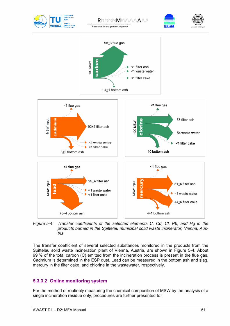
University of Stuttgart
AWAST D1 – D2: MFA Manual 61
carbon
98+3 flue gas
<1 filter cake
<1 waste water<1 filter ash
1,4+1 bottom ash10
0 M
SW
carbon
98+3 flue gas
<1 filter cake
<1 waste water<1 filter ash
1,4+1 bottom ash10
0 M
SW
cadm
ium
<1 filter cake<1 waste water
92+2 filter ash
8+2 bottom ash
<1 flue gas
MSW
Inpu
t
cadm
ium
<1 filter cake<1 waste water
92+2 filter ash
8+2 bottom ash
<1 flue gas
MSW
Inpu
t
clorine
<1 flue gas
<1 filter cake
54 waste water
37 filter ash
10 bottom ash
100
MSW
clorine
<1 flue gas
<1 filter cake
54 waste water
37 filter ash
10 bottom ash
100
MSW
clorine
<1 flue gas
<1 filter cake
54 waste water
37 filter ash
10 bottom ash
100
MSW
lead
25+4 filter ash
<1 filter cake<1 waste water
75+4 bottom ash
MSW
Inpu
t
<1 flue gas
lead
25+4 filter ash
<1 filter cake<1 waste water
75+4 bottom ash
MSW
Inpu
t
<1 flue gas
lead
25+4 filter ash
<1 filter cake<1 waste water
75+4 bottom ash
MSW
Inpu
t
<1 flue gas
mercury
<1 waste water
4+1 bottom ash
51+6 filter ash
44+6 filter cake
<1 flue gas
MSW
Inpu
t
mercury
<1 waste water
4+1 bottom ash
51+6 filter ash
44+6 filter cake
<1 flue gas
MSW
Inpu
t
Figure 5-4: Transfer coefficients of the selected elements C, Cd, Cl, Pb, and Hg in the
products burned in the Spittelau municipal solid waste incinerator, Vienna, Aus-tria
The transfer coefficient of several selected substances monitored in the products from the Spittelau solid waste incineration plant of Vienna, Austria, are shown in Figure 5-4. About 99 % of the total carbon (C) emitted from the incineration process is present in the flue gas. Cadmium is determined in the ESP dust. Lead can be measured in the bottom ash and slag, mercury in the filter cake, and chlorine in the wastewater, respectively. 5.3.3.2 Online monitoring system
For the method of routinely measuring the chemical composition of MSW by the analysis of a single incineration residue only, procedures are further presented to:
University of Stuttgart
AWAST D1 – D2: MFA Manual 62
select the appropriate incineration residue to be analyzed determine the minimum sampling frequency of the residue analyze the chemical composition of MSW routinely with a given accuracy
The method developed by Morf and Brunner [Morf & Brunner, 1998] allows to use waste in-cineration plants as an analytical tool for quality control in waste management. Mass bal-ances of selected substances are determined experimentally by a series of investigations of the municipal solid waste incineration plant, as follows: Investigation I: - a provisional material balance of the solid waste incineration plant is established to de-
termine the orders of magnitude of the material concentrations and material flows Investigation II: - mass balances of the selected elements are performed during 48 h with separately col-
lected household waste as the incinerator feed Investigation III: - mass balances of the selected substances are performed during 48 h with ordinary,
mixed municipal solid waste as the incinerator feed Investigation IV: - a certain number of additional filter ash samples are analyzed during a period of 12
months to determine statistical parameters like time constants and variances for the se-lected substances
In investigations I – III, the flows through the incinerator of all input goods (e.g. MSW) and output goods (bottom ash, scrap metals, filter ash, wastewater, filter cake, flue gas) have to be measured. Determination of the incineration residue best suited for waste composition monitoring Due to their homogeneity, substance enrichment and accessibility, the different residues of incineration offer various possibilities to determine the waste composition. In order to select the best suited incineration residue for a certain element, the following procedures are sug-gested. The design of the incineration plant, available resources, and desired accuracy influence the choice of the appropriate incineration residue. For MSW incineration, the ratio of the mass flow of the incinerator residue versus the waste input has to be a minimum. The partitioning of the investigated element from the waste input into the chosen incinerator residue (transfer coefficient) has to be a maximum. For the metals investigated, the influence of the concentration level of the chosen incineration residue and the variation of the transfer coefficient are nearly negligible. The variation of the concentra-tion in the residue considered has to be a minimum. As a result, a homogenous incineration residue with a low specific mass output rate and a high accumulation rate with minimum variance is to be preferred for monitoring waste composition. Ideally, these conditions are fulfilled for many substances in a single incineration residue. In order to select the best suited incineration residue, to design the sampling strategy, and subsequently to calculate the waste composition, the following parameters have to be deter-mined experimentally:
the transfer coefficients of the selected substances into the relevant residues the variation of transfer coefficients the variance of the concentration
University of Stuttgart
AWAST D1 – D2: MFA Manual 63
the time constant of the considered system expressing the degree of correlation Determination of the sampling frequency Fewer samples are needed to determine the mean composition of a lot for internally or auto-correlated than for lots consisting of randomly distributed components. A lot is a finite part of a process, e.g. a waste stream during one year. A process with a degree of correlation equal to zero (expressed by the time constant) is to-tally uncorrelated (a random process). Here the time variance component of the total vari-ance is large compared to the variability due to sample heterogeneity, sample preparation, and analysis. A process with the time constant → ∞ is totally correlated, respectively. For a process with a high value of the time constant, both a small sampling size fraction and a small number of samples are needed to describe the lot with sufficient accuracy. For a proc-ess with a very low time constant, only the relative size of the gross sample is determining. Therefore, it is unimportant whether the relative size of the gross sample is obtained by tak-ing many small samples or one large sample. Factors causing this correlation can depend upon time as well as on space, e.g., changing waste properties due to new consumer prod-ucts. Since the concentrations of the investigated substance in the waste stream are not meas-ured, but the concentrations are determined from a corresponding and appropriate incinera-tion residue, some equations are used to determine the sampling strategy for this residue. The uncertainty of the mean waste composition is then estimated by the variance which cor-responds to the optimum sampling strategy. Determination of waste composition by the analysis of a single incineration residue The mean concentration for an element in waste input is calculated by using:
the measured mass flows of the residue and the waste input the mean concentration of the investigated element measured in the residue the mean transfer coefficient of the investigated substance for the corresponding resi-
due To calculate the uncertainty of the mean concentration of the investigated substance in the waste input, the general law of propagation of error is applied. For a solid waste incineration, it can be generally assumed that the variance of routinely measured waste and residue mass flows and any covariance terms are negligible.
Table 5-4: Mean transfer coefficients (with ~95 % confidence interval) determined in the Spittelau municipal solid waste incineration plant, Vienna, Austria, 1994
Cu Zn Cd Pb
bottom ash 0.94 ± 0.01 0.43 ± 0.03 0.08 ± 0.02 0.75 ± 0.04
ESP dust 0.06 ± 0.01 0.57 ± 0.03 0.92 ± 0.02 0.25 ± 0.04
filter cake < 0.01 < 0.01 < 0.01 < 0.01
wastewater < 0.01 < 0.01 < 0.01 < 0.01
flue gas < 0.01 < 0.01 < 0.01 < 0.01
Table 5-4 shows the mean transfer coefficients (with approximate 95 % confidence interval) determined in the Spittelau municipal solid waste incinerator. The values are based on inves-
University of Stuttgart
AWAST D1 – D2: MFA Manual 64
tigation III and the application of the law of propagation of error without considering variances of mass and covariance terms. With the exception of lead, the mean values of the transfer coefficients are comparable (relative difference less than ±10 %) with results of other meas-uring campaigns on MSW incinerators. The mean transfer coefficients appear to depend on the applied technology and the plant design. This hypothesis is supported by a comparison of the results with other measurements and with measurements on a MSW incinerator plant with similar state of the art technology but a different plant design (e.g., type of grate, geome-try of combustion chamber, operating control). It is assumed that the partitioning of metals in MSW incinerators depends on the waste input and the incineration process. Up to now, this hypothesis cannot be tested with the available data. The rather low level of uncertainty in Table 5-4 is due to a well-designed sampling plan for the measuring campaign. Nearly 100 % of the input flow of the four selected metals (Cu, Zn, Cd, and Pb) is transferred into the two incineration residues bottom ash and ESP dust. This is due to state of the art technology applied in the Spittelau municipal solid waste incinerator. The two residues are possible monitoring goods for the selected metals. Further investigations have been carried out to distinguish which of the two residues is best suited for each metal. Hourly composite samples (five samples of two kg each per hour) of bottom ash as well as ESP dust (four samples of two kg each per hour) were taken. The composite samples were homogenized, and two samples of the same size were taken and pulverized. Duplicate analysis was performed on each pulverized sample. When comparing the approximate 95 % confidence interval of the waste composition calculated with bottom ash on the one hand and with ESP dust on the other hand, the following has to be considered: Bottom ash was sam-pled during 19 one hour measuring periods (38 total number of samples), and ESP dust was sampled only during 15 one hour periods (30 total number of samples). This enhanced pro-gram for the sampling of bottom ash has been chosen based on the results of investigation I, which showed that the filter ash was more homogenous than the bottom ash. Taking this into account and since ESP dust is a material easy to sample and to pretreat for analysis, ESP dust serves best to determine Cd, Pb, and Zn in the waste feed. Approximate uncertainty for the calculated waste composition is equal or less than 20 % for all selected metals. Cad-mium, which is highly enriched in ESP dust, can be determined even more accurately. The time constants and the variances for the four selected substances (Cu, Zn, Cd, and Pb) have been determined in investigation IV. ESP dust has been sampled every second week for five days during the time period of 1 year. Twice a day, a 12-h composite sample was taken, consisting of four 1.5-kg grab samples each. The composite samples were homoge-nized, subsampled, and prepared for analysis. Two samples were analyzed. In total, 256 mean concentration values for the selected metals evenly distributed during a one year pe-riod were determined. The calculation model for minimizing the sampling frequency was ap-plied to this data. The autocorrelation functions were calculated for the time series of all four metals. All measurements were included for the calculations. No transformation was applied to the data sets. The time constants and the variances were determined with the autocorrela-tion functions of the time series approximated with an exponential function. The parameters determined in investigation IV were applied to the calculation model for minimizing the sampling frequency to evaluate the uncertainty of the mean waste composi-tion as a function of the number of samples in the ESP dust. With a sampling period of 365 days, one analysis per sample, and the variance of analysis equal to 0.02*process variance (as determined in investigation III), the approximate relative 95 % confidence intervals were calculated for the mean ESP dust concentration during the defined time period as a function of the sampling frequency.
University of Stuttgart
AWAST D1 – D2: MFA Manual 65
To assure a relative error width of less than 10 %, with a 95 % confidence for all four se-lected metals, approximately 30 ESP dust samples have to be taken during one year. The final choice of the optimal number of samples is due to considerations regarding accepted uncertainty for the mean waste composition for the selected elements and costs. The influence of the sampling size on the results discussed above is shown by the example of Cd. With a sampling period of 365 days, one analysis per sample, the variance of analysis equal to 0.02*process variance, and the same reference values for Cd as the obtained re-sults, the effect of the sampling size on the result was calculated. By increasing the sampling size, the uncertainty level can be kept constant with a significantly decreased number of samples. This means that the best sampling strategy is to take a few samples only (2-3) per month over a full year. In practice, the sampling strategy is determined by the uncertainty accepted, the reliability of sampling equipment for long sampling periods, and the costs of sampling and analysis. By applying the calculation model for the determination of waste composition, with a sam-pling period of 365 days, sampling size << 1 day, one analysis per sample, and the variance of analysis equal to 0.02*process variance, the approximate relative 95 % confidence interval was calculated for the mean waste concentration during the defined time period as a function of the sampling frequency. Depending on the sampling strategy, the uncertainty of the mean concentration for the se-lected metals can be kept small. Due to an increased sampling effort, the variance of the mean concentration of the investigated element in the residue is minimized, which, according to an equation of the calculation model applied, results in lower values of the mean concen-tration for the two elements Cd and Zn. Thus, the annual mean concentration for all four in-vestigated metals can be determined accurately for a reasonable annual number of samples by the proposed method. Applying the method and the obtained results in practice, the MSW incinerator Spittelau serves as a fine tool to monitor routinely and cost effectively the concen-trations of selected metals in the municipal solid waste of Vienna, Austria. The Austrian experience shows that the method can be extended to other substances (e.g., carbon monitored in the flue gas, chlorine monitored in the wastewater). For all substances studied in investigations I-IV, the uncertainty level of the annual mean remains in the range of the results obtained. It is essential to use good data, to select the appropriate incineration residue, and to design an optimal sampling strategy for each element in order to assure rea-sonable uncertainty levels. Up to now, the hypothesis for a generalization of the results has not been verified yet. Therefore, determination of the sampling frequency and determination of the incineration residue best suited for waste composition monitoring have to be applied for every new plant to assure defined uncertainty levels for the estimators of the means. Fur-ther investigations about the dependency of transfer coefficients on the waste input, process conditions, and plant design, as well as on the time series of elemental concentrations in the waste stream may help to reduce sampling and costs. 5.3.3.3 Potentials and limitations of the analysis of waste treatment products
The major advantage consists in the fact that the analysis of waste treatment products is well suited for the determination of the elemental concentration of municipal solid waste. Espe-cially in the case of substances present at low concentrations, the method is the best way to get reliable information on municipal solid waste composition. This is demonstrated by the substance mercury which derives mainly from batteries. It is time consuming and requires very large quantities of MSW to find the few batteries which make up the mercury content of
University of Stuttgart
AWAST D1 – D2: MFA Manual 66
a few milligrams per kilogram of MSW, and it is even more difficult to produce a representa-tive laboratory sample suited for mercury analysis without losing most of the mercury during sample size reduction and preparation. In an incineration, about 75 % of the incoming mer-cury is transferred to the gas and can be accurately measured semi-continuously [Brunner & Mönch, 1986]. Another advantage of this method is the homogenizing effect of the treatment process. The incinerator acts as a large “thermal digester” and releases products which have a more uni-form composition than the initial MSW. Also, the incinerator concentrates certain elements in specific products of small volumes (e.g. Cadmium in the ESP dust) and it becomes therefore possible to follow the concentration of this element in MSW over a long period of time by the periodic analysis of ESP dust, if the partitioning of this metal between the products of incin-eration is known [Brunner & Mönch, 1986]. In any case, the expense for sampling and analysis to characterize a large amount of MSW (> 10 tonnes) is always larger for the “direct waste analysis” than for the “waste product analysis”. The main disadvantage of the waste product analysis is the fact that the determination of materials is generally not accomplished, e.g. it is not possible to calculate the contents of paper, plastic or other organic substances from the composition of the products from incin-eration. This means that, in most cases, the product method is limited to the analysis of ele-mental composition and parameters like energy content, water content, content of total inor-ganic and organic matter. 5.4 Conclusions
The successful management of MSW depends upon the knowledge of MSW composition. Decisions on recycling, optimization of waste treatment processes and predictions of emis-sions from waste treatment are among the many reasons that there is a need to know the content of materials and elements in MSW. The three different methods to analyse MSW discussed above have different applications and properties. It is of chief importance to choose the method of analysis which is most appropriate for the objectives of a particular question of waste management. In general, the direct waste analysis yields good results on some materials in MSW, but it is difficult and very labour intensive to determine substance concentrations by this method. The waste product analysis is well suited for the determina-tion of the substance concentration of MSW but in most cases does not allow analysing the material composition. The market product analysis is an efficient method to determine mate-rial and substance composition of MSW, and, therefore in combination with the waste prod-uct analysis is able to replace the direct waste analysis.
University of Stuttgart
AWAST D1 – D2: MFA Manual 67
6 Examples
The examples of “Thermal Treatment“, “Mechanical – Biological Waste Treatment“, “Landfill“ and “Waste Collection“ were selected as examples. They are expected to serve for: 1. identi-fying the processes and fluxes of relevance for each case study, 2. orientation towards the relevance of particular goods and substance fluxes. The average values outlined in each case study can be considered as orientation values. It should be taken into account that for certain specific facilities, some single values might quite deviate from their particular average value. 6.1 Thermal Treatment
In this chapter, three technologies of thermal treatment are presented. Among these, the most relevant for the solid waste management is the waste incineration in grate furnaces. Further, industrial waste incineration in fluidised bed incinerators and industrial incineration in rotary shaft kilns, as in the cement industry, are described. 6.1.1 Waste Incineration in Grate Furnace Incinerators
Incinerators have been employed for decades in the waste management. Municipal solid wastes from the private households and industrial wastes similar to them are usually inciner-ated there without pre-treatment. Compared to the late Sixties, off-gas treatment has been significantly improved. The general scheme and operation of a waste incinerator can be described by means of few facility components and aggregates. The latter are offered by a variety of producers, as large as the spectre of the particular design. Among these however, incineration principle and sub-stance flows hardly differ. Figure 6-7 demonstrates the construction scheme of a waste incinerator. There, the following function sections are represented:
Waste reception Storage, Pre-treatment (Homogenisation) Loading and Incineration Unit Bottom Ash Withdrawal, (optionally – Residue Treatment), Storage Furnace, Steam Utilisation Off-gas Treatment Wastewater Treatment Unit Optionally - Residue Treatment Chimney

University of Stuttgart
AWAST D1 – D2: MFA Manual 68
E. Schachermayer, 1995Grafik: Inge Hengl/EGAB/anlage.dsf
feed bell
waste bunker
furnace
electro-filter
bottom ashremoval
fly ash removal
treated wastewater
off-gaswashers
scrapbottom ash
magnet tapeconveyor
DeNOx
WTP
purifiedoff-gas
fly ash
filter cake
Figure 6-1: Construction scheme of a waste incinerator
6.1.1.1 Functioning of a Waste Incineration Plant (Vienna, Spittelau)
The waste collection truck is weighed at the entrance of the waste incineration plant (WIP) and then unloaded into a waste bunker. The weight control serves the estimation of the waste amount delivered and further mainly the fee billing. Since waste delivery occurs discontinuing (only on working days) on the contrary to waste incinerator feeding, a storage possibility should exist for the waste delivered. The waste bun-ker serves waste buffering and homogenising, where a gripping crane mixes the wastes. The crane can further enable a rough waste pre-treatment for bulky waste, so that the need of an additional facility for waste pre-treatment is avoided. For preventing odour and dust emis-sions, in the waste bunker (and as far as available in the waste unloading station) slight low-pressure is secured. The exhausted air is fed into the incineration as primary air. The waste is forwarded by means of a gripping crane into the feed bell. The latter serves as an interim storage for the continuous feeding of the incineration unit. Grate furnaces enable a steady waste throughput, since the kiln runs can be continuously conveyed. Further, targeted oxygen supply and adequate motion of the wastes during incineration are to be secured. A variety of grate furnace systems has been developed for incinerating household wastes and similar industrial wastes (advance grates, back grates and roller grates). Independently of the grate system applied, the principle construction of the incineration space is limited downwards by the incineration grate, sideward by the walls and upwards by a ceiling or a kettle.

University of Stuttgart
AWAST D1 – D2: MFA Manual 69
The incineration process can be divided in several phases that however cannot be unequivo-cally demarcated from each other:
Drying phase: at a temperature of 100 °C, the water is separated from the waste. Degasification phase: by further heating to 250 °C, the volatile substances are de-
sorbed. These are in first line residual moisture, hydrocarbons and tar. Gasification phase: at temperatures over 500 °C, the oxidation takes place less at the
grate itself but in the incineration space and in the post-incineration zone. Incineration phase: the flammable gases from the previous processes get fully oxidised
at temperatures over 800 °C. Post-incineration phase: secures a faultless burnout.
At the end of the grate, the bottom ash is gravitationally dropped out and cooled by employ-ing wet systems. After this, metal scrap is separated by a magnet tape. The bottom ash is disposed on residue landfills, the metal scrap is forwarded to the blast furnace process. For the off-gas treatment to follow, the off-gas is to be cooled from over 1,000 °C down to ca. 200 °C. The released heat can be utilised for producing warm water, saturated vapour and superheated steam for distance heating. The latter two can be also employed for electricity production. Incineration of one tone household wastes results in ca. 4,000 to 5,000 Nm³ off-gas. Along with the typical incineration gaseous products (CO, CO2, H2O, SO2, NOx ), polluters depend-ing on the waste composition occur as well. These are mainly hydrogen chlorides and fluo-rides, dust, heavy metals as well as hydrocarbons (e.g. dioxins and furans). Single air pollutants occur as gases or particles. During the off-gas treatment, particles are generally first eliminated, and just afterwards – the gaseous contaminants. A diversity of technologies is available for the (raw) off-gas purification. Through the chimney the purified off-gas is finally let out in the atmosphere. The next section describes one off-gas purification system, as installed at the Spittelau waste incineration plant in Vienna. The dust is removed from the cooled raw off-gas in the electro-filter. Here, dust particles get negatively charged and remain at the positively charged separator. An electro-filter is capa-ble of catching even smallest particles and thus secures high separation rates. Here in the flying ash, mainly heavy metals such as cadmium are concentrated. Finally, the dust-free raw off-gas passes through a vacuum pump, so to get saturated with water vapour and cooled down to ca. 60 °C. Afterwards, it is twice washed. In the acid washer where chemicals and water are added, mainly hydrogen chlorides and fluorides are eliminated from the off-gas. A part of the water is fed as circulating, another one is regularly separated. The strongly acid wastewater is fed into the internal wastewater treatment plant, in a first step of neutralisation and a second for flocculating and sedimenting the particles. The neutralisation sludge (filter cake) contains, among the rest, mercury as well and is to be thus disposed on underground landfills. In the neutral or alkaline washer, SO2 is eliminated by applying sodium hydroxide and further, in the internal wastewater treatment plant, converted into gypsum. For the following catalytic denitrification (DeNOx), the washed raw off-gas is to be warmed again. With ammonia, the nitrogen oxides are reduced to N2 and H2O. The purified off-gas leaves the incineration plant passing the chimney.
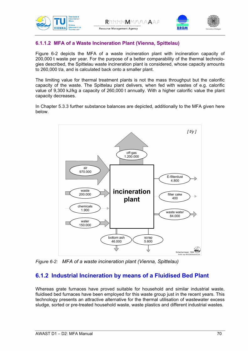
University of Stuttgart
AWAST D1 – D2: MFA Manual 70
6.1.1.2 MFA of a Waste Incineration Plant (Vienna, Spittelau)
Figure 6-2 depicts the MFA of a waste incineration plant with incineration capacity of 200,000 t waste per year. For the purpose of a better comparability of the thermal technolo-gies described, the Spittelau waste incineration plant is considered, whose capacity amounts to 260,000 t/a, and is calculated back onto a smaller plant. The limiting value for thermal treatment plants is not the mass throughput but the calorific capacity of the waste. The Spittelau plant delivers, when fed with wastes of e.g. calorific value of 9,300 kJ/kg a capacity of 260,000 t annually. With a higher calorific value the plant capacity decreases. In Chapter 5.3.3 further substance balances are depicted, additionally to the MFA given here below.
Schachermayer, 1994Grafik: Inge 98\EGAB\blackbox.dsf
incinerationplant
off-gas1.200.000
bottom ash46.000
scrap5.600
air970.000
chemicals1.900
water150.000
E-filterdust4.800
filter cake400
waste water84.000
waste200.000
[ t/y ]
Figure 6-2: MFA of a waste incineration plant (Vienna, Spittelau) 6.1.2 Industrial Incineration by means of a Fluidised Bed Plant
Whereas grate furnaces have proved suitable for household and similar industrial waste, fluidised bed furnaces have been employed for this waste group just in the recent years. This technology presents an attractive alternative for the thermal utilisation of wastewater excess sludge, sorted or pre-treated household waste, waste plastics and different industrial wastes.
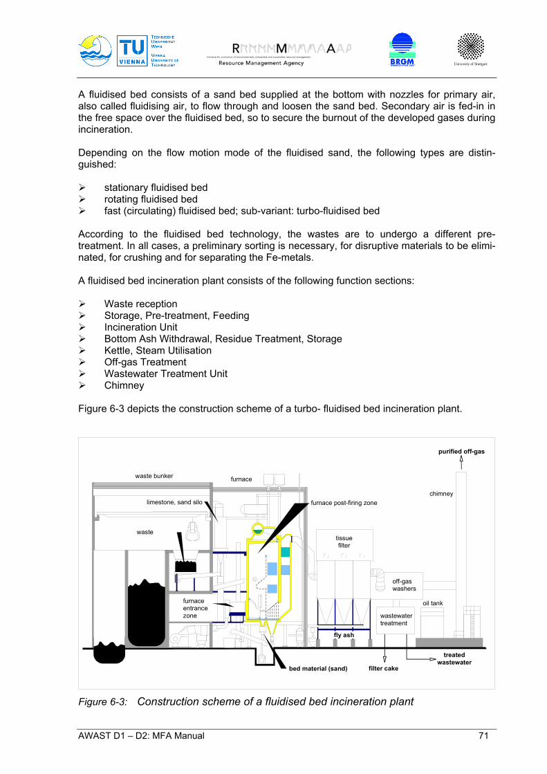
University of Stuttgart
AWAST D1 – D2: MFA Manual 71
A fluidised bed consists of a sand bed supplied at the bottom with nozzles for primary air, also called fluidising air, to flow through and loosen the sand bed. Secondary air is fed-in in the free space over the fluidised bed, so to secure the burnout of the developed gases during incineration. Depending on the flow motion mode of the fluidised sand, the following types are distin-guished:
stationary fluidised bed rotating fluidised bed fast (circulating) fluidised bed; sub-variant: turbo-fluidised bed
According to the fluidised bed technology, the wastes are to undergo a different pre-treatment. In all cases, a preliminary sorting is necessary, for disruptive materials to be elimi-nated, for crushing and for separating the Fe-metals. A fluidised bed incineration plant consists of the following function sections:
Waste reception Storage, Pre-treatment, Feeding Incineration Unit Bottom Ash Withdrawal, Residue Treatment, Storage Kettle, Steam Utilisation Off-gas Treatment Wastewater Treatment Unit Chimney
Figure 6-3 depicts the construction scheme of a turbo- fluidised bed incineration plant.
waste
limestone, sand silo
furnace entrancezone
tissuefilter
chimney
fly ash
oil tank
furnace post-firing zone
bed material (sand)
furnacewaste bunker
purified off-gas
wastewatertreatment
treatedwastewater
filter cake
off-gaswashers
Figure 6-3: Construction scheme of a fluidised bed incineration plant
University of Stuttgart
AWAST D1 – D2: MFA Manual 72
6.1.2.1 Functioning of Fluidised Bed Incineration Plant
An Austrian development to the turbo-fluidised bed incineration is described below. It has been constructed particularly for the thermal utilisation of waste and problematic materials. The most significant feature of the turbo-fluidised bed is the location of the fluidised bed and the post-incineration chamber. When delivered, the waste is weighed and undergoes a reception control. According to the aggregate state of the wastes, different interim storage bunkers are employed (sludge bun-kers for wastewater excess sludge and bunkers for residues, such as waste plastics, waste wood, pre-treated household wastes, light fraction). If necessary, the wastes from the bun-kers for residues are to be first crushed in a shredder and sieved prior to their being fed into the incineration. The wastewater treatment excess sludge is forwarded by means of a gripping crane from its bunker into the wastewater treatment excess sludge silo, and the residues – into the residue silo. From these two silos, both waste mixtures advance (e.g. by a dosing worm) onto a common conveyor. Onto the latter, quartz sand and lime can be added if necessary. The waste mixture is then fed into the firing by means of an aerated feeder. The turbo-fluidised bed is highly suitable for wastes proving great differences in their calorific value, since the sand bed is an excellent warm accumulator and thus a suitable buffer for energy fluctuations. In this technology, the fluidised bed is divided into two zones: The en-trance zone is only slightly supplied with incineration air, whereas the incineration zone is extremely intensively aerated. The fluidised bed has an open nozzle bottom, and primary air is blown through. It first sets the sand bed in motion, and then also serves as incineration air. The primary air can be pre-heated up to 650 °C, so to enable the compensation of fluctuations of the calorific value of the kiln run. Next to the nozzle bottom, the rough ash is continuously withdrawn. The waste mixture enters over the slightly aerated zone and follows the motion of the fluid-ised bed. This way, it becomes dried, degasified and gasified within a very short time period. It then proceeds into the incineration zone where, with secondary air being blown in, the in-cineration occurs at temperatures of ca. 850 °C to 900 °C. The solids are eliminated from the off-gas by a particle separator and fall off onto the en-trance zone below. This sand rain mixes up with the wastes continuously fed in and supports their blending with the fluidised bed. The incineration products set free in the incineration zone rise over the entrance zone in a mixing zone (turbulence zone). There they meet the off-gas which, after the particle separa-tor, is free of bed material and rich of oxygen. Thanks to the high flow velocity, a highly fa-vourable mixing occurs. In the post-incineration chamber, the complete burnout of the off-gases takes place. The first dust elimination step occurs in a separator where dust particles larger than 0.1 mm of diameter are led back to the fluidised bed. The equipment employed for the off-gas purifi-cation is similar to the ones in the waste incineration plants. The off-gas is first cooled in the boiler, with the energy set free being utilised. Then, the further purification takes place, by means of tissue or electro-filters, washers and denitrificators. The wastewater from the two washers is treated as in a waste incineration plant. The purified off-gas leaves the fluidized bed plant over the chimney.
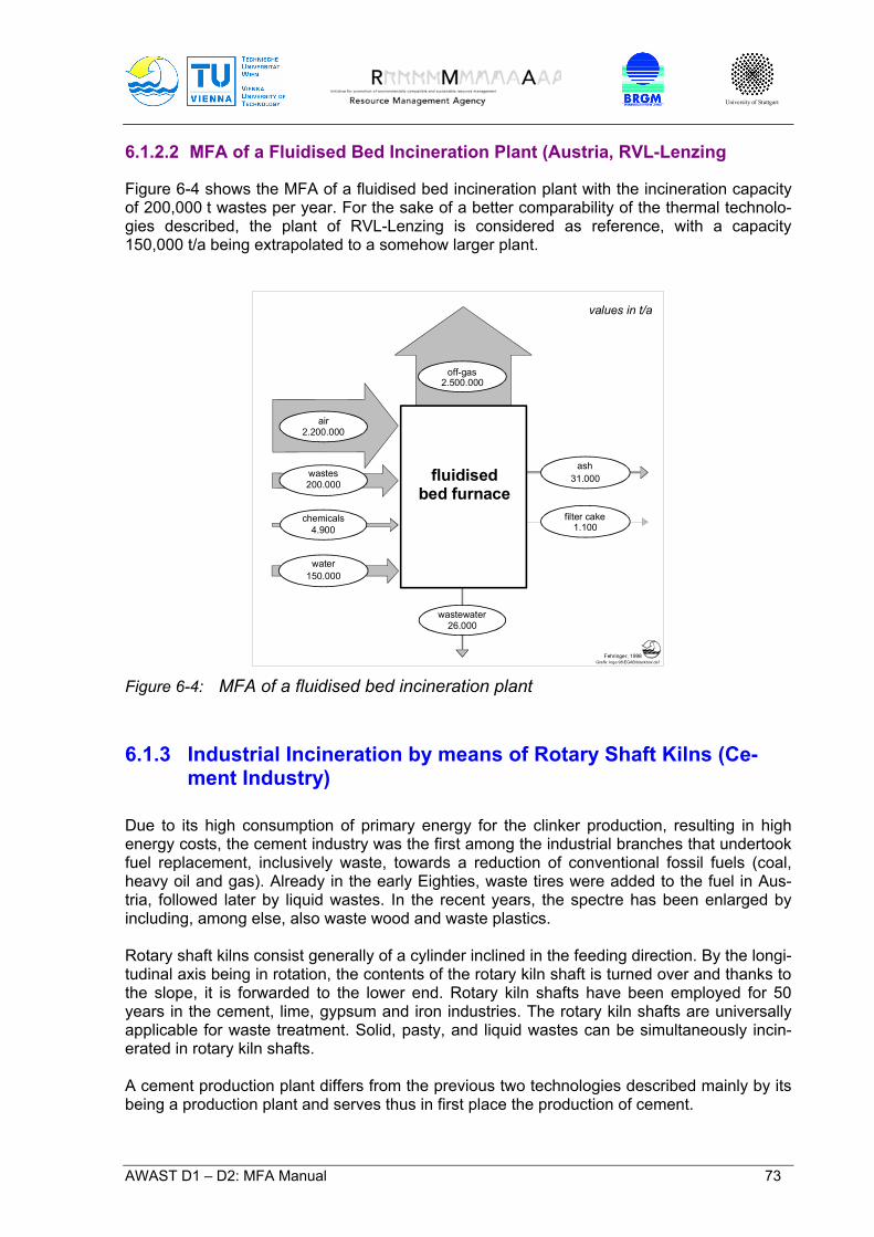
University of Stuttgart
AWAST D1 – D2: MFA Manual 73
6.1.2.2 MFA of a Fluidised Bed Incineration Plant (Austria, RVL-Lenzing
Figure 6-4 shows the MFA of a fluidised bed incineration plant with the incineration capacity of 200,000 t wastes per year. For the sake of a better comparability of the thermal technolo-gies described, the plant of RVL-Lenzing is considered as reference, with a capacity 150,000 t/a being extrapolated to a somehow larger plant.
Fehringer, 1998Grafik: Inge 98\EGAB\blackbox.dsf
2.500.000
150.000
26.000
2.200.000
4.900
31.000200.000
1.100
air
wastes
chemicals
water
off-gas
wastewater
ash
filter cake
values in t/a
fluidisedbed furnace
Figure 6-4: MFA of a fluidised bed incineration plant 6.1.3 Industrial Incineration by means of Rotary Shaft Kilns (Ce-
ment Industry)
Due to its high consumption of primary energy for the clinker production, resulting in high energy costs, the cement industry was the first among the industrial branches that undertook fuel replacement, inclusively waste, towards a reduction of conventional fossil fuels (coal, heavy oil and gas). Already in the early Eighties, waste tires were added to the fuel in Aus-tria, followed later by liquid wastes. In the recent years, the spectre has been enlarged by including, among else, also waste wood and waste plastics. Rotary shaft kilns consist generally of a cylinder inclined in the feeding direction. By the longi-tudinal axis being in rotation, the contents of the rotary kiln shaft is turned over and thanks to the slope, it is forwarded to the lower end. Rotary kiln shafts have been employed for 50 years in the cement, lime, gypsum and iron industries. The rotary kiln shafts are universally applicable for waste treatment. Solid, pasty, and liquid wastes can be simultaneously incin-erated in rotary kiln shafts. A cement production plant differs from the previous two technologies described mainly by its being a production plant and serves thus in first place the production of cement.
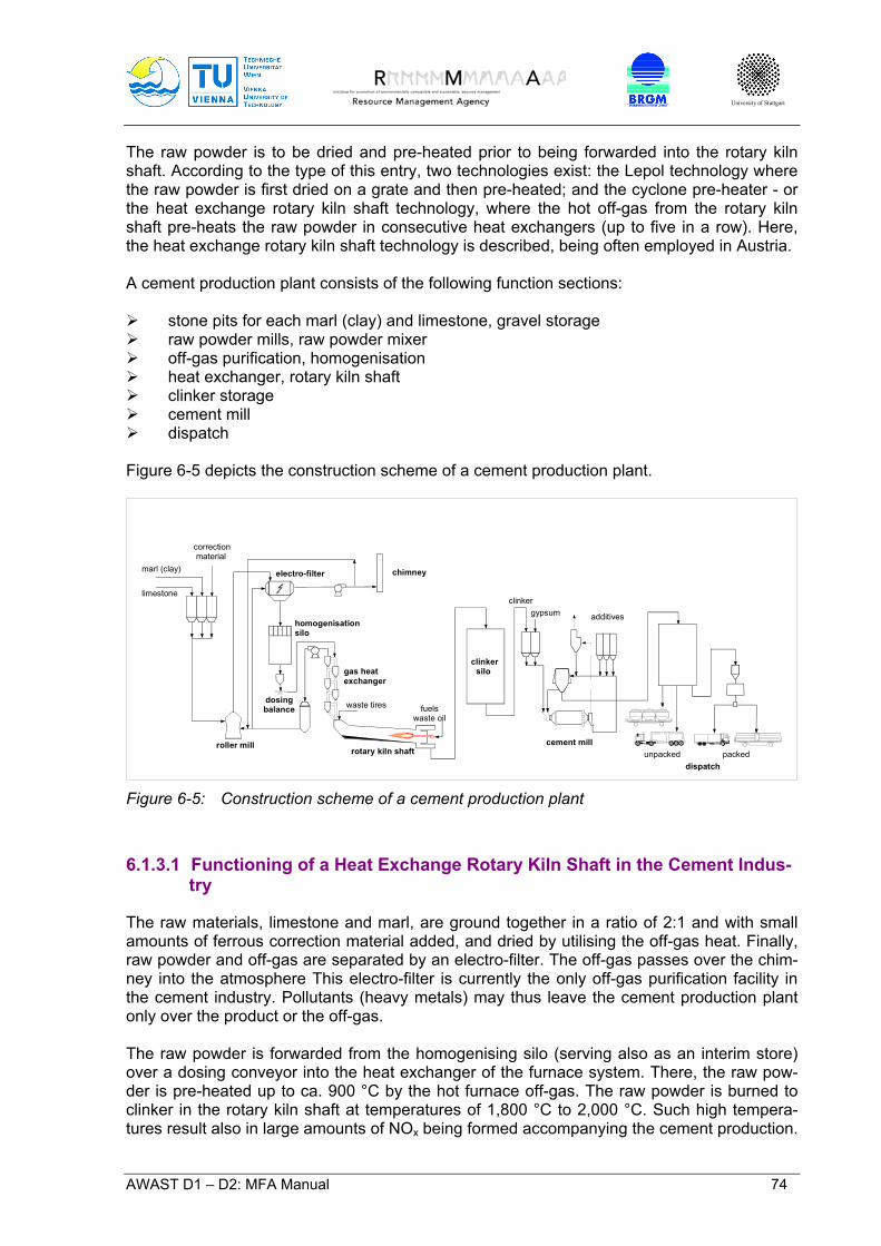
University of Stuttgart
AWAST D1 – D2: MFA Manual 74
The raw powder is to be dried and pre-heated prior to being forwarded into the rotary kiln shaft. According to the type of this entry, two technologies exist: the Lepol technology where the raw powder is first dried on a grate and then pre-heated; and the cyclone pre-heater - or the heat exchange rotary kiln shaft technology, where the hot off-gas from the rotary kiln shaft pre-heats the raw powder in consecutive heat exchangers (up to five in a row). Here, the heat exchange rotary kiln shaft technology is described, being often employed in Austria. A cement production plant consists of the following function sections:
stone pits for each marl (clay) and limestone, gravel storage raw powder mills, raw powder mixer off-gas purification, homogenisation heat exchanger, rotary kiln shaft clinker storage cement mill dispatch
Figure 6-5 depicts the construction scheme of a cement production plant.
marl (clay)
limestone
correctionmaterial
chimneyelectro-filter
homogenisationsilo
gas heatexchanger
waste tires
roller mill
dosingbalance
rotary kiln shaft
clinker silo
clinkergypsum additives
dispatchpackedunpacked
cement mill
fuelswaste oil
Figure 6-5: Construction scheme of a cement production plant
6.1.3.1 Functioning of a Heat Exchange Rotary Kiln Shaft in the Cement Indus-
try
The raw materials, limestone and marl, are ground together in a ratio of 2:1 and with small amounts of ferrous correction material added, and dried by utilising the off-gas heat. Finally, raw powder and off-gas are separated by an electro-filter. The off-gas passes over the chim-ney into the atmosphere This electro-filter is currently the only off-gas purification facility in the cement industry. Pollutants (heavy metals) may thus leave the cement production plant only over the product or the off-gas. The raw powder is forwarded from the homogenising silo (serving also as an interim store) over a dosing conveyor into the heat exchanger of the furnace system. There, the raw pow-der is pre-heated up to ca. 900 °C by the hot furnace off-gas. The raw powder is burned to clinker in the rotary kiln shaft at temperatures of 1,800 °C to 2,000 °C. Such high tempera-tures result also in large amounts of NOx being formed accompanying the cement production.
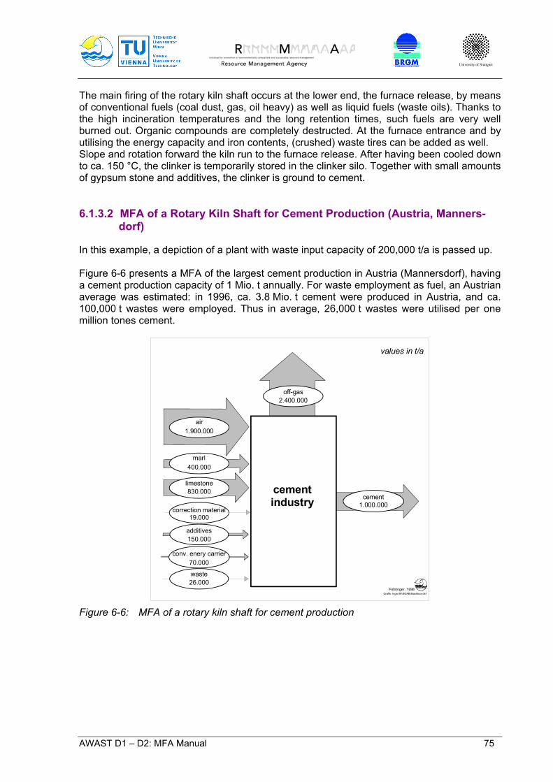
University of Stuttgart
AWAST D1 – D2: MFA Manual 75
The main firing of the rotary kiln shaft occurs at the lower end, the furnace release, by means of conventional fuels (coal dust, gas, oil heavy) as well as liquid fuels (waste oils). Thanks to the high incineration temperatures and the long retention times, such fuels are very well burned out. Organic compounds are completely destructed. At the furnace entrance and by utilising the energy capacity and iron contents, (crushed) waste tires can be added as well. Slope and rotation forward the kiln run to the furnace release. After having been cooled down to ca. 150 °C, the clinker is temporarily stored in the clinker silo. Together with small amounts of gypsum stone and additives, the clinker is ground to cement. 6.1.3.2 MFA of a Rotary Kiln Shaft for Cement Production (Austria, Manners-
dorf)
In this example, a depiction of a plant with waste input capacity of 200,000 t/a is passed up. Figure 6-6 presents a MFA of the largest cement production in Austria (Mannersdorf), having a cement production capacity of 1 Mio. t annually. For waste employment as fuel, an Austrian average was estimated: in 1996, ca. 3.8 Mio. t cement were produced in Austria, and ca. 100,000 t wastes were employed. Thus in average, 26,000 t wastes were utilised per one million tones cement.
Fehringer, 1998Grafik: Inge 98\EGAB\blackbox.dsf
2.400.000
70.000
26.000
1.900.000
830.000
150.000
1.000.000
400.000
19.000
air
marl
limestone
correction material
additives
conv. enery carrier
waste
cement industry cement
values in t/a
off-gas
Figure 6-6: MFA of a rotary kiln shaft for cement production

University of Stuttgart
AWAST D1 – D2: MFA Manual 76
6.2 Mechanical Biological Waste Treatment
6.2.1 Introduction
6.2.1.1 Functioning of a Facility for Mechanical Biological Waste Treatment
The technical options to construct a facility for mechanical biological waste treatment are manifold. This allows for the practical combination of any possible technology accorded to the local circumstances. A common feature of all them is that thanks to the treatment, the output material quality towards disposal perspectives is significantly changed compared to the input material quality. For example, the Austrian Landfill Act defines a mechanical biological waste pre-treatment, as follows: A mechanical biological waste pre-treatment is a technological combination of mechanical and biological processes for waste pre-treatment. The goal of the mechanical processes is to separate the material less appropriate for a biological treatment as well as to eliminate dis-ruptive material and pollutants as well as to optimise the biological degradation of the resid-ual material by increasing their homogeneity and biological availability. The goal of the bio-logical processes is the deepest possible degradation of organic matter (degradation and transformation of biologically degradable components by employing anaerobic – aerobic or aerobic technologies. Mechanically biologically pre-treated wastes are characterised by a significant reduction of their volume, water contents and gas building potential as well as by a significant improvement of their leaching and settling behaviour. [BGBl 164/1996, 1996] The mechanical facilities serve the material processing for the biological stage. The me-chanical stage should:
Eliminate disruptive materials (e.g. stones, very large components, dangerous wastes, foamed plastics as CFC carrier)
Separate materials not appropriate for a biological treatment (e.g. plastics, siev-ing residues of a high calorific content, metals)
Homogenise and condition the material, i.e. supply it with enough porosity, enough water contents and nutrient distribution to secure an optimal progress of the biological degradation. [Mostbauer et al., 1998]
The mechanical stage of the facility includes, among others, crushing machines, sieves, drum sieves, mixing drums, magnet separators, irrigation facilities. The biological stage serves the microbiological degradation and the transformation of the mechanically processed material. Here, both aerobic and anaerobic technologies are possi-ble to apply. During the anaerobic treatment (fermentation) the organic substance is degraded in the absence of air, at temperatures between 30° and 55°C, and with a minimum water content of >60 %. The facility can be designed as a single- or multistage reactor. The retention time of the material in the reactor amounts to in total ca. 1-3 weeks. The treatment product is biogas and part of the input fraction that remains slowly degradable under anaerobic conditions (hy-drolysis product).
University of Stuttgart
AWAST D1 – D2: MFA Manual 77
The biogas consists of 50-85 % methane (CH4). The rest is presented by carbon dioxide (CO2), with traces of H2S, H2, CO, NH3. This gas can be utilised as energy, covering the en-ergy demand of the facility. Energy excess is usually fed into the public electrical network. However, gaining an output material of low reactivity and thus well disposable at a landfill, the dewatered hydrolysis product is to undergo an aerobic treatment (2 - 5 weeks). Facility equipment (air insulation, gas collection, large liquor amounts) and its operative maintenance (constant temperature, sensitive micro organisms) are, compared to an aerobic unit, relatively intensive. The advantages of the fermentation process are that it allows for processing pasty and liquid organic wastes as well; and, appropriate operation management secured, the energy con-sumption of the entire facility is over-compensated by the biogas. Under the aerobic treatment (rotting) the organic matter is degraded, in the presence of oxygen, finally to CO2, water and inorganic compounds. The first step of the treatment is ho-mogenisation and adjusting the optimal water content by adding water or digested sludge from the wastewater treatment plants. This step takes ca. 1 - 2 days. The following main treatment step, the degradation process, lasts for ca. 6-12 weeks. The heat produced by it heats up the matter up to 70°C. The last two treatment steps are usually performed indoor. By adjusting temperature, air supply and moisture the degradation conditions are optimised and the process progress can be controlled. The following post-degradation takes place out-door and lasts for up to several months depending on treatment target – volume reduction or gas potential reduction. This step determines the final degradation grade of the organic mat-ter and thus its reactivity. Eventually, a repeated separation of fractions of high calorific value and disruptive substance may be performed between the main treatment and the post-degradation. In a rough approximation, it can be stated that the mechanical biological treatment reduces the material for landfilling down to approximately one third related to the input mass. One third is degraded microbiologically, and one third is separated as pollutants or utilisable ma-terial. The latter should undergo an appropriate further disposal or, respectively, treatment. Compared to residual wastes, the material that has undergone a mechanical biological treatment proves a lower gas building potential and better qualities towards its settling and leaching behaviour. 6.2.1.2 Legal Framework in Europe
The EU- Landfill Directive [Directive 1999/31/EC, 1999] was passed in 1999 by the Council of Ministers. Among others, it sets the amount of biologically degradable municipal wastes to be gradually reduced until 2015 down to 35 % related to the mass in 1995. Further, minimum standards are set regarding waste evaluation, and the demand is agreed upon as to landfill construction and its monitoring by the country members. Concerning waste categorisation into different landfill classes, it is required to restrict future landfilling only to pre-treated wastes. Mixing different waste types is strictly prohibited, so to secure keeping the prescribed limit values. In Germany, waste management procedures are generally settled by material cycle legisla-tion acts and the Waste Management Act (KrW-/AbfG). However, since the object of these regulations is only presented by landfills and similar facilities, a mechanical biological treat-ment is only considered in the context of landfilling. Waste utilisation facilities, waste incin-

University of Stuttgart
AWAST D1 – D2: MFA Manual 78
eration plants, sorting units and mechanical biological facilities are licensed similarly to indus-trial facilities, i.e. by applying the Federal Immission Protection Law (BimSchG). Waste categorisation towards landfill classes is performed by applying the Technical Manual for Municipal Wastes (TASi). It states the requirements to the material, the landfill and to the leachate. Normally, the required organic burn-up loss of 5 %, the content of total organic car-bon (TOC) of 3 % in the solid phase and 100 mg/l in the leachate are exceeded for materials after a mechanical biological treatment. However, starting 1. 6. 2005, no more exceptions like these will be allowed [Zeschmar-Lahl et al., 2000]. The regulations in Italy admit both thermal and mechanical biological waste pre-treatment technologies. The matter to landfill shall not exceed the limit values of 35 % for degradable organic substance and of 400 mg O2/kg dried solids for respiratory activity. These limit values were set in 1997, by allowing a transition period till 1.1.2000. [Zeschmar-Lahl et al., 2000] According to Mostbauer [Mostbauer et al., 1998], the limit value AT7of 15 mg O2/g dried sol-ids (equal to 15.000 mg O2/kg dried solids) is suggested for mechanically biologically treated wastes in Austria. This means that in Italy as well, mechanically biologically pre-treated mu-nicipal wastes cannot be landfilled except by a special permit granted. Legal preconditions for constructing, operating and licensing a facility for mechanical biologi-cal facilities (MBA) in Austria are just being elaborated aiming at a “Technical Manual MBA“ [Mostbauer et al., 1998]. The Austrian Landfill Ordinance (DVO) [BGBl 164/1996, 1996] pro-hibits to landfill wastes proving a TOC value higher than 5 %. This limit value cannot be achieved by means of the mechanical biological treatment. Therefore, the wastes treated this way are excepted from this prohibition if their upper calorific value Ho does not exceed 6.000 kJ/kg. For existing facilities, these regulations are obligatory starting in 2004 [BGBl 325/1990, 1990]. 6.2.2 Case Study Aerobic Mechanical Biological Treatment of Re-
sidual Wastes (Residual Waste Treatment Plant Allerheiligen - Austria)
The Allerheiligen plant has been investigated on behalf of the Federal Ministry of Environ-ment, Youth and Family and of the Provincial government of Styria [Harant et al., 1999]. The plant is located in the Mürztal, in the Austrian province of Styria, and is operated by the Waste Network of Mürz (the Mürzverbund). In the framework of this study, goods and sub-stance flows have been investigated gaining data material through samples and measure-ments in the period from June 1997 till April 1998. The study objective was to investigate the substance flows of a facility for mechanical biological waste treatment, so to enable forecasts on input, transformation and output paths. That would be of relevance for planning and opti-mising of real facilities. The balances for the following parameters were supposed to be cal-culated: moist solids, dried solids, organic burn-up loss, total organic carbon, biodegradable organic dried substance, upper calorific value, polycyclic aromatic carbohydrates, organic halogen compounds respectively, total carbohydrates as well as for the heavy metals lead, cadmium and zinc.
University of Stuttgart
AWAST D1 – D2: MFA Manual 79
6.2.2.1 System Definition
Allerheiligen Facility Description The Allerheiligen plant consists of two treatment lines for bio-wastes (6,500 t/a) and for re-sidual wastes under addition of digested sludge from the wastewater treatment (17,100 t/a + 5,000 t/a). This study concentrates on investigating the residual wastes – sludge – mixture only. The residual waste is weighed on a bridge balance when delivered, and proceeds to a bun-ker. A gripper forwards it into the hammer mill. Next, the iron particles are separated by a magnet separator. Afterwards, the wastes pass through a drum sieve with a mesh width of 80 mm. The fraction bigger than 80 mm and being of high calorific value does not undergo any further treatment but sorts out by being directly landfilled. The rest of the residual waste being <80 mm is mixed with digested sludge from the waste-water treatment. The mixing ratio residual waste to sludge differs depending on the water content of the wastes in the range between 65:35 and 80:20. Approximately 100 t of the waste-sludge mixture are fed into the intensive rotting stage constructed as aerated BAS rotting-tunnels. The plant disposes over 9 tunnels, 6 of which serve the residual waste treat-ment, and 3 – the bio-waste processing. Oxygen and temperature are controlled by varying the air supply. The tunnel aeration amounts up to 10,000 m3 air/h. Since the water balance of the rotting process is negative, additional moisture is fed in as fresh water and as leachate from the intensive and extensive rotting units. Leaving the rotting tunnel, the waste material is treated within further 4 weeks on vacuum-aerated rotting plates (extensive rotting). During the extensive rotting, the charge is neither being mixed nor turned nor moistened. That is why the water content of the matter usually sinks below 30 %. Due to the lack of space the treatment normally ends by this unit and the matter is landfilled. Only for this project, a post-extensive treatment stage lasting for 16 weeks was added. For this purpose, ca. 15 % (ca. 7-10 t) of the material were taken out of each process charge and piled up without aeration. The mass is turned up and moistened every 2 weeks. After a total treatment of 22 weeks, the material was sieved into 3 fractions (80-24 mm, 24-12 mm, <12 mm), and all 3 fractions were then landfilled. Defining the spatial system boundary The system includes the plant for mechanical biological treatment. Processes like delivering of residual waste, digested sludge and process water, the further treatment and the product disposal (metals, light fraction, treated matter, off-gas) lie all outside the system boundary and are thus not regarded. Defining the temporal system boundary As a temporal system boundary, the period of 1 year is selected. A continuous data measur-ing exceeding this period is not possible. The annual freights are thus extrapolated out of the punctual measurement values.
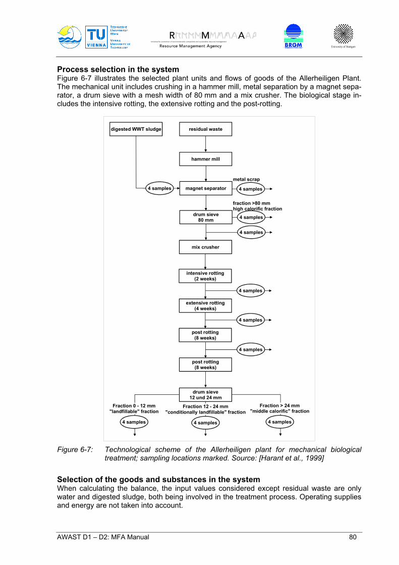
University of Stuttgart
AWAST D1 – D2: MFA Manual 80
Process selection in the system Figure 6-7 illustrates the selected plant units and flows of goods of the Allerheiligen Plant. The mechanical unit includes crushing in a hammer mill, metal separation by a magnet sepa-rator, a drum sieve with a mesh width of 80 mm and a mix crusher. The biological stage in-cludes the intensive rotting, the extensive rotting and the post-rotting.
digested WWT sludge residual waste
hammer mill
magnet separator
drum sieve80 mm
mix crusher
metal scrap
4 samples
fraction >80 mmhigh calorific fraction
4 samples
4 samples
4 samples
intensive rotting(2 weeks)
4 samples
extensive rotting(4 weeks)
4 samples
post rotting(8 weeks)
4 samples
post rotting(8 weeks)
drum sieve12 und 24 mm
4 samples
Fraction 12 - 24 mm"conditionally landfillable" fraction
4 samples
Fraction 0 - 12 mm"landfillable" fraction
4 samples
Fraction > 24 mm"middle calorific" fraction
Figure 6-7: Technological scheme of the Allerheiligen plant for mechanical biological
treatment; sampling locations marked. Source: [Harant et al., 1999]
Selection of the goods and substances in the system When calculating the balance, the input values considered except residual waste are only water and digested sludge, both being involved in the treatment process. Operating supplies and energy are not taken into account.

University of Stuttgart
AWAST D1 – D2: MFA Manual 81
The focus of the output in the balance is set on the solid goods (metal scrap, fraction of high calorific content, rotting products of different time points). Sampling and analysis concern exclusively these solids as well. Goods and substance flows over wastewater and off-gas are indirectly considered through the balances of the solids. 6.2.2.2 Determining the Goods and Substance Fluxes
Sampling The sampling approach plays a crucial role for the results derived in the project. Sampling such inhomogeneous material like residual wastes requires a 5 l sample from a charge mass up to 160 m3 (ca. 100 t) taken in a manner that secures the sample would be the representa-tive for the whole material towards its elemental composition and chemical qualities. From these 5 l, only a part is further used for analysing the parameters of interest (cr. Table 6-1).
Table 6-1: The following amounts are analysed from a 100 t charge mass:
Parameter Sample amount Dried solids DS 1,000 g Organic burn-up loss OBL 10-20 g TOC 3-4 mg Upper calorific value Ho some g biodegradable organic dried substance oDSbio no data polycyclic aromatic carbohydrates PAK 10-15 g organic halogen compounds POX 30 g Total carbohydrates max. 0.5 g Pb, Cd, Zn each 0.25 g
Residual waste composition strongly varies within a year. Since the residual wastes for this plant origin from an agricultural region, an increase of inert substances can be detected dur-ing the cold seasons. Also, the degradation conditions (temperature and moisture of the sur-rounding air and in the tunnels) vary with the season. Therefore, 12 different tunnel charge samples were taken within 4 weeks in the research year. The residual waste fraction >80 mm contains a large amount of textile and plastic objects of which even a single one not crushed would fill the sampling box. To gain a representative sample though, several kilos of the high-calorific fraction were taken out with the gripper and manually crushed. Afterwards, the mass was shrunk by cross-mixing down to 5 l. The paral-lel samples were taken in ca. 30 –minute-intervals. With regard to the Fe-metals, corresponding material was being collected at the end of the conveyor until the sample volume of 5 l was gained. Crushing and homogenisation of ac-ceptable effort were not possible, and thus not performed. The residual waste fraction <80 mm was temporarily stored in piles before its being mixed with the digested sludge. The samples were taken by shovels when the material was being fed into the mix crusher until a wheel barrow (ca. 100 l) was filled. The samples originated from the layers over the pile cross-section. The content of six wheel barrows was mixed to-gether and shrunk down by the diagonal approach, until a sample of 5 l was left. The digested sludge from the municipal wastewater treatment is a relatively homogenous mass, thus the samples were taken directly from the feeding shaft before the mix crusher. The samples at the end of the intensive rotting were taken from the conveyor when the material was being exported from the tunnel. The matter originating from its front sections
University of Stuttgart
AWAST D1 – D2: MFA Manual 82
was exported prior to the one from the back sections. In the progress of this export, 4-6 wheel barrows were collected and mixed. After cross-mixing, a sample of 5 l was taken. The samples at the end of the extensive rotting and in the middle of the post-rotting were taken in the same manner as for the residual waste <80 mm. The fine, middle and rough fractions of the rotting material at the end of the post-rotting is very homogenous. The 5 l samples were taken directly from the outlet shaft of the sieve. The off-gas of the plant was sampled only once. Sample analysis The mass fluxes were determined by weighing each total charge of residual waste fraction <80 mm during their being turned up by the wheel loader. The masses of the metals and residual wastes >80 mm thrown out were determined through the balance calculation for the entire plant. At 4 of all 12 tunnels all goods fluxes were sampled (cr. Figure 6-7), and within the pollutant analysis programme, all parameters (MS, DS, OBL, TOC, oDSbio, Ho, PAK, POX resp. total carbohydrates, Pb, Cd, Zn) were analysed. For the rest of 8 charges, the fraction >80 mm and the metal scrap were not sampled; for the other samples, only the basic analysis pro-gramme was performed, i.e. without analysing the pollutants (oDSbio, PAK, POX resp. total carbohydrates, Pb, Cd, Zn). Within the pollutant analysis programme, 4 parallel samples were taken for each material charge sampled. Within the basic analysis programme it were 3 parallel samples. Mass Balance and Result Interpretation The mass balance is based on the weighing measurements. By considering the analytical parameters, the single balances for each of them are gained. 6.2.2.3 Results for the Allerheiligen Plant for mechanical biological treatment
Table 6-2: Input-output balances of the Allerheiligen plant for mechanical biological treat-ment, [Harant et al., 1999]
INPUT Water
Intensive rotting
Water Post-rotting
Digested sludge (DS)
Residual waste (RW) Input DS + RW
Moist solids (MS) 35.6 % 17.8 % 23.9 % 76.1 % 1,394.5 t Dried solids (DS) 10.3 % 89.7 % 764.5 t Organic burn-up loss (OBL) 12.9 % 87.1 % 430.0 t TOC 11.8 % 88.2 % 255.0 t Upper calorific value Ho 12.1 % 87.9 % 10,893.0 GJ Biodegr. org. dried sub-stance oDSbio
15.8 % 84.2 % 112.9 t
Polycycl. arom. carbohydr. PAK 7.4 % 92.6 % 1.96 kg
Digested Sludge + Residual Waste = 100 %
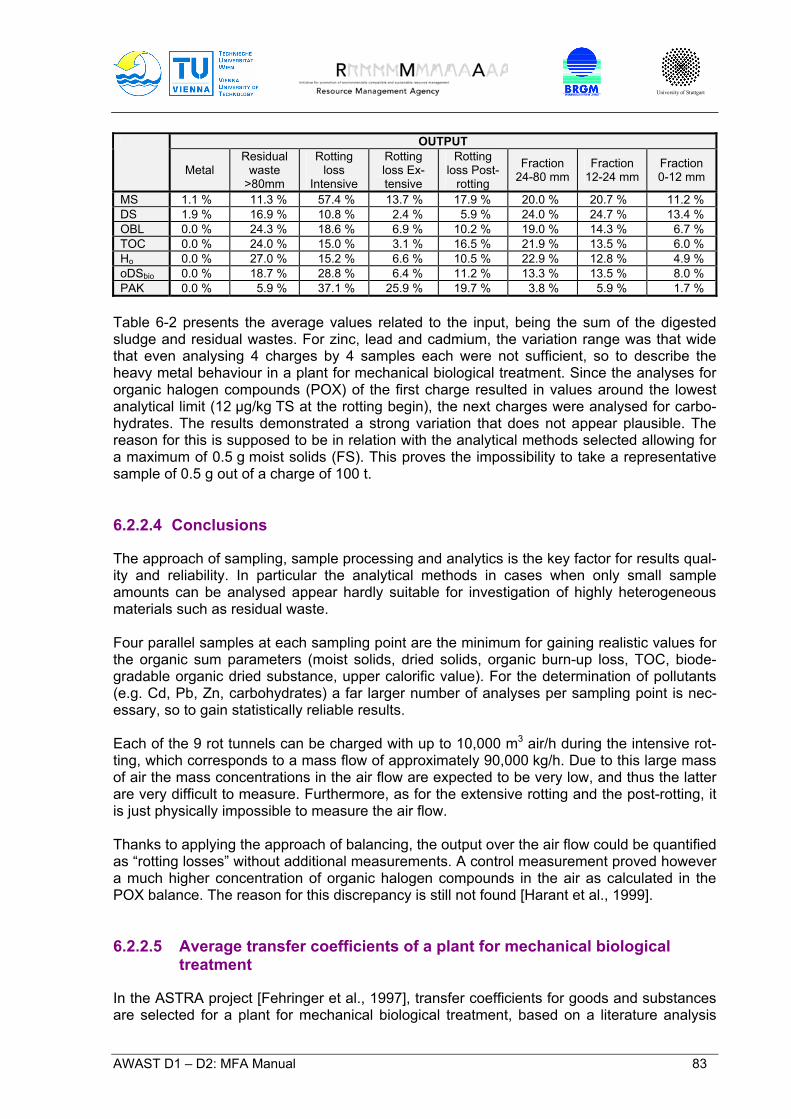
University of Stuttgart
AWAST D1 – D2: MFA Manual 83
OUTPUT
Metal Residual
waste >80mm
Rotting loss
Intensive
Rotting loss Ex-tensive
Rotting loss Post-
rotting
Fraction 24-80 mm
Fraction 12-24 mm
Fraction 0-12 mm
MS 1.1 % 11.3 % 57.4 % 13.7 % 17.9 % 20.0 % 20.7 % 11.2 % DS 1.9 % 16.9 % 10.8 % 2.4 % 5.9 % 24.0 % 24.7 % 13.4 % OBL 0.0 % 24.3 % 18.6 % 6.9 % 10.2 % 19.0 % 14.3 % 6.7 % TOC 0.0 % 24.0 % 15.0 % 3.1 % 16.5 % 21.9 % 13.5 % 6.0 % Ho 0.0 % 27.0 % 15.2 % 6.6 % 10.5 % 22.9 % 12.8 % 4.9 % oDSbio 0.0 % 18.7 % 28.8 % 6.4 % 11.2 % 13.3 % 13.5 % 8.0 % PAK 0.0 % 5.9 % 37.1 % 25.9 % 19.7 % 3.8 % 5.9 % 1.7 %
Table 6-2 presents the average values related to the input, being the sum of the digested sludge and residual wastes. For zinc, lead and cadmium, the variation range was that wide that even analysing 4 charges by 4 samples each were not sufficient, so to describe the heavy metal behaviour in a plant for mechanical biological treatment. Since the analyses for organic halogen compounds (POX) of the first charge resulted in values around the lowest analytical limit (12 µg/kg TS at the rotting begin), the next charges were analysed for carbo-hydrates. The results demonstrated a strong variation that does not appear plausible. The reason for this is supposed to be in relation with the analytical methods selected allowing for a maximum of 0.5 g moist solids (FS). This proves the impossibility to take a representative sample of 0.5 g out of a charge of 100 t. 6.2.2.4 Conclusions
The approach of sampling, sample processing and analytics is the key factor for results qual-ity and reliability. In particular the analytical methods in cases when only small sample amounts can be analysed appear hardly suitable for investigation of highly heterogeneous materials such as residual waste. Four parallel samples at each sampling point are the minimum for gaining realistic values for the organic sum parameters (moist solids, dried solids, organic burn-up loss, TOC, biode-gradable organic dried substance, upper calorific value). For the determination of pollutants (e.g. Cd, Pb, Zn, carbohydrates) a far larger number of analyses per sampling point is nec-essary, so to gain statistically reliable results. Each of the 9 rot tunnels can be charged with up to 10,000 m3 air/h during the intensive rot-ting, which corresponds to a mass flow of approximately 90,000 kg/h. Due to this large mass of air the mass concentrations in the air flow are expected to be very low, and thus the latter are very difficult to measure. Furthermore, as for the extensive rotting and the post-rotting, it is just physically impossible to measure the air flow. Thanks to applying the approach of balancing, the output over the air flow could be quantified as “rotting losses” without additional measurements. A control measurement proved however a much higher concentration of organic halogen compounds in the air as calculated in the POX balance. The reason for this discrepancy is still not found [Harant et al., 1999]. 6.2.2.5 Average transfer coefficients of a plant for mechanical biological
treatment
In the ASTRA project [Fehringer et al., 1997], transfer coefficients for goods and substances are selected for a plant for mechanical biological treatment, based on a literature analysis
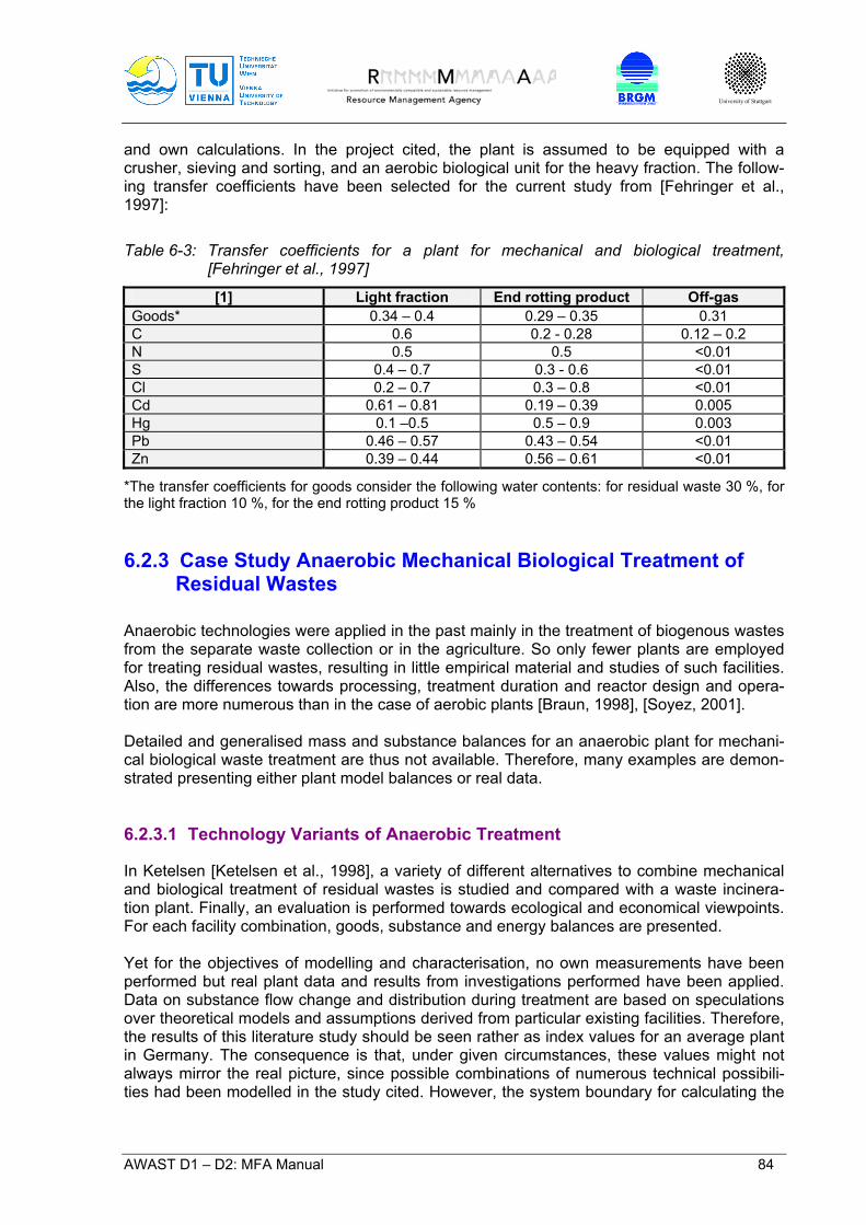
University of Stuttgart
AWAST D1 – D2: MFA Manual 84
and own calculations. In the project cited, the plant is assumed to be equipped with a crusher, sieving and sorting, and an aerobic biological unit for the heavy fraction. The follow-ing transfer coefficients have been selected for the current study from [Fehringer et al., 1997]:
Table 6-3: Transfer coefficients for a plant for mechanical and biological treatment, [Fehringer et al., 1997]
[1] Light fraction End rotting product Off-gas Goods* 0.34 – 0.4 0.29 – 0.35 0.31 C 0.6 0.2 - 0.28 0.12 – 0.2 N 0.5 0.5 <0.01 S 0.4 – 0.7 0.3 - 0.6 <0.01 Cl 0.2 – 0.7 0.3 – 0.8 <0.01 Cd 0.61 – 0.81 0.19 – 0.39 0.005 Hg 0.1 –0.5 0.5 – 0.9 0.003 Pb 0.46 – 0.57 0.43 – 0.54 <0.01 Zn 0.39 – 0.44 0.56 – 0.61 <0.01
*The transfer coefficients for goods consider the following water contents: for residual waste 30 %, for the light fraction 10 %, for the end rotting product 15 % 6.2.3 Case Study Anaerobic Mechanical Biological Treatment of
Residual Wastes
Anaerobic technologies were applied in the past mainly in the treatment of biogenous wastes from the separate waste collection or in the agriculture. So only fewer plants are employed for treating residual wastes, resulting in little empirical material and studies of such facilities. Also, the differences towards processing, treatment duration and reactor design and opera-tion are more numerous than in the case of aerobic plants [Braun, 1998], [Soyez, 2001]. Detailed and generalised mass and substance balances for an anaerobic plant for mechani-cal biological waste treatment are thus not available. Therefore, many examples are demon-strated presenting either plant model balances or real data. 6.2.3.1 Technology Variants of Anaerobic Treatment
In Ketelsen [Ketelsen et al., 1998], a variety of different alternatives to combine mechanical and biological treatment of residual wastes is studied and compared with a waste incinera-tion plant. Finally, an evaluation is performed towards ecological and economical viewpoints. For each facility combination, goods, substance and energy balances are presented. Yet for the objectives of modelling and characterisation, no own measurements have been performed but real plant data and results from investigations performed have been applied. Data on substance flow change and distribution during treatment are based on speculations over theoretical models and assumptions derived from particular existing facilities. Therefore, the results of this literature study should be seen rather as index values for an average plant in Germany. The consequence is that, under given circumstances, these values might not always mirror the real picture, since possible combinations of numerous technical possibili-ties had been modelled in the study cited. However, the system boundary for calculating the
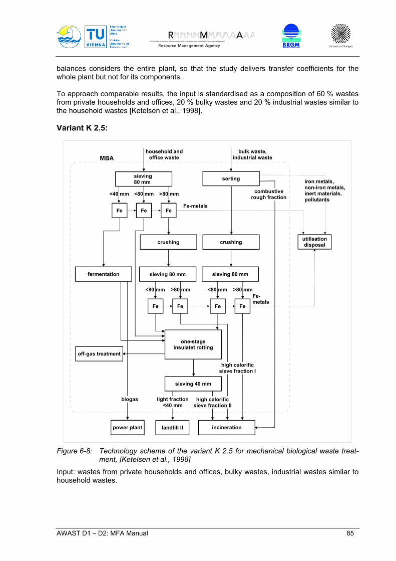
University of Stuttgart
AWAST D1 – D2: MFA Manual 85
balances considers the entire plant, so that the study delivers transfer coefficients for the whole plant but not for its components. To approach comparable results, the input is standardised as a composition of 60 % wastes from private households and offices, 20 % bulky wastes and 20 % industrial wastes similar to the household wastes [Ketelsen et al., 1998]. Variant K 2.5:
household andoffice waste
bulk waste, industrial waste
sorting
Fe
crushing
one-stageinsulatet rotting
sieving80 mm
FeFe
<40 mm <80 mm >80 mm
MBA
crushing
sieving 80 mm sieving 80 mmfermentation
FeFe
<80 mm >80 mm
FeFe
<80 mm >80 mmFe-metals
iron metals,non-iron metals,inert materials,pollutants
off-gas treatment
sieving 40 mm
light fraction<40 mm
high calorificsieve fraction II
Fe-metals
landfill II incineration
high calorificsieve fraction I
biogas
power plant
utilisationdisposal
combustiverough fraction
Figure 6-8: Technology scheme of the variant K 2.5 for mechanical biological waste treat-
ment, [Ketelsen et al., 1998]
Input: wastes from private households and offices, bulky wastes, industrial wastes similar to household wastes.
University of Stuttgart
AWAST D1 – D2: MFA Manual 86
Mechanical pre-treatment prior to the biological unit: sorting, crushing, sieving and iron sepa-ration, in two lines for household and office wastes as well as for bulky wastes and industrial wastes similar to household wastes. Biological treatment: Anaerobic treatment of the fraction < 40 mm in the household and office wastes. Aerobic treatment for the fermentation residues for the fraction 40-80 mm of the household and office wastes and of the fraction < 80 mm of the bulky and industrial wastes similar to household wastes. Mechanical after-rotting treatment: the product is separated into a landfill fraction < 40 mm and a fraction of high calorific value. The fractions > 80 mm separated in the mechanical unit prior to biological treatment for all three waste groups considered are foreseen as high calorific fractions destinated to thermal final treatment. Variants K 2.6 and K 2.7
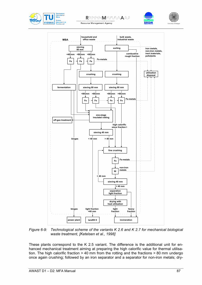
University of Stuttgart
AWAST D1 – D2: MFA Manual 87
household andoffice waste
bulk waste, industrial waste
sorting
Fe
crushing
one-stageinsulatet rotting
sieving80 mm
FeFe
<40 mm <80 mm >80 mm
MBA
crushing
sieving 80 mm sieving 80 mmfermentation
FeFe
<80 mm >80 mm
FeFe
<80 mm >80 mm
iron metals,non-iron metals,inert materials,pollutants
off-gas treatment
sieving 40 mm
< 40 mm
Fe-metals
landfill II incineration
high calorificsieve fraction I
biogas
power plant
utilisationdisposal
fine crushing
> 40 mm
Fe
NI
Fe-metals
non-ironmetals
sieving 40 mm
> 40 mm
separationlight fraction
drying withheat utilisation
Fe-metals
light fraction<40 mm
lightfraction
biogas
< 40 mm
heavyfraction
combustiverough fraction
Figure 6-9: Technological scheme of the variants K 2.6 and K 2.7 for mechanical biological
waste treatment, [Ketelsen et al., 1998]
These plants correspond to the K 2.5 variant. The difference is the additional unit for en-hanced mechanical treatment aiming at preparing the high calorific value for thermal utilisa-tion. The high calorific fraction > 40 mm from the rotting and the fractions > 80 mm undergo once again crushing; followed by an iron separator and a separator for non-iron metals; dry-
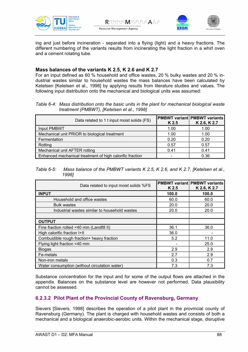
University of Stuttgart
AWAST D1 – D2: MFA Manual 88
ing and just before incineration - separated into a flying (light) and a heavy fractions. The different numbering of the variants results from incinerating the light fraction in a whirl oven and a cement rotating tube. Mass balances of the variants K 2.5, K 2.6 and K 2.7 For an input defined as 60 % household and office wastes, 20 % bulky wastes and 20 % in-dustrial wastes similar to household wastes the mass balances have been calculated by Ketelsen [Ketelsen et al., 1998] by applying results from literature studies and values. The following input distribution onto the mechanical and biological units was assumed:
Table 6-4: Mass distribution onto the basic units in the plant for mechanical biological waste treatment (PMBWT), [Ketelsen et al., 1998]
Data related to 1 t input moist solids (FS) PMBWT variant K 2.5
PMBWT variants K 2.6, K 2.7
Input PMBWT 1.00 1.00 Mechanical unit PRIOR to biological treatment 1.00 1.00 Fermentation 0.20 0.20 Rotting 0.57 0.57 Mechanical unit AFTER rotting 0.41 0.41 Enhanced mechanical treatment of high calorific fraction - 0.36
Table 6-5: Mass balance of the PMBWT variants K 2.5, K 2.6, and K 2.7, [Ketelsen et al., 1998]
Data related to input moist solids %FS PMBWT variant K 2.5
PMBWT variants K 2.6, K 2.7
INPUT 100.0 100.0 Household and office wastes 60.0 60.0 Bulk wastes 20.0 20.0 Industrial wastes similar to household wastes 20.0 20.0 OUTPUT Fine fraction rotted <40 mm (Landfill II) 36.1 36.0 High calorific fraction I+II 36.0 - Combustible rough fraction+ heavy fraction 5.2 11.0 Flying light fraction <40 mm - 25.0 Biogas 2.9 2.9 Fe-metals 2.7 2.9 Non-iron metals 0.3 0.7 Water consumption (without circulation water) 7.3 7.3
Substance concentration for the input and for some of the output flows are attached in the appendix. Balances on the substance level are however not performed. Data plausibility cannot be assessed. 6.2.3.2 Pilot Plant of the Provincial County of Ravensburg, Germany
Sievers [Sievers, 1998] describes the operation of a pilot plant in the provincial county of Ravensburg (Germany). The plant is charged with household wastes and consists of both a mechanical and a biological anaerobic-aerobic units. Within the mechanical stage, disruptive

University of Stuttgart
AWAST D1 – D2: MFA Manual 89
materials, metals and plastic films are separated in a light fraction. The organic fraction is crushed prior to the biological treatment into solids <20 mm and is homogenised. The latter fraction is mixed with water and then treated anaerobically. The fermentation resi-dues are dewatered in press units and aerobically stabilised in closed containers and in aer-ated piles.
Table 6-6 Plant data for the Ravensburg PMBWT [Sievers, 1998]
Ravensburg PMBWT Fermentation type Dry fermentation (ca. 35 % dried solidsTS) Anaerobic units 1 Reactor volume 44 m3
Temperature range of the units mesophilic to theromphilic (35-45°C resp. 45-60°C) Anaerobic treatment duration 21 d Aerobic treatment duration No data
Table 6-7 Mass balance Ravensburg PMBWT [Sievers, 1998]
Ravensburg PMBWT [% moist solids, FS] [t/a]* INPUT Residual wastes 100 % 1,250 OUTPUT mechanical unit Disruptive substances 10 % 125 Utilisable materials, plastic films, metals 26 % 325 OUTPUT biological unit Biogas 9 % 113 Rotting losses post-rotting (incl. drying) 20 % 250 Residues 35 % 438
* Approximation calculated as 5 t/d, 250 operation days/a 6.2.3.3 Model Derived from the Münster PMBWT, Germany
A comparison between fermentation and rotting has been illustrated by a fictive plant and its balance calculation by Ibrahim [Ibrahim, 1998], served by an existing plant in Münster as a prototype. The plant simulation foresees dewatering of the fermentation residue and a closed circulation for the process wastewater pressed out there. The PMBWT is fed with residual wastes. The mechanical stage separates 70 % of the input as a rough fraction which is di-rectly forwarded to the rotting process. The other 30 % of the fine fraction are fed into the conditioning container of the anaerobic unit. In this container, the fine fraction is diluted up to 10 – 15 % dried solids (DS), and floating and settling materials are separated as well. The following step is a mesophilic fermentation tank. After a retention time of 16 – 20 days in the latter, the product is dewatered and mineralised in an aerobic process (rotting). Table 6-8 presents the mass balance of this plant, viewing the moist solids (MS), dried solids (DS) and organic dried solids (oDS).
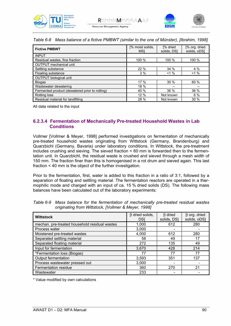
University of Stuttgart
AWAST D1 – D2: MFA Manual 90
Table 6-8 Mass balance of a fictive PMBWT (similar to the one of Münster), [Ibrahim, 1998]
Fictive PMBWT [% moist solids, MS]
[% dried solids, DS]
[% org. dried solids, oDS]
INPUT Residual wastes, fine fraction 100 % 100 % 100 % OUTPUT mechanical unit Settling substance 22 % 34 % 4 % Floating substance 3 % <1 % <1 % OUTPUT biological unit Biogas 17 % 30 % 60 % Wastewater dewatering 18 % -- -- Fermented product (dewatered prior to rotting) 40 % 36 % 36 % Rotting loss 12 % Not known 6 % Residual material for landfilling 28 % Not known 30 %
All data related to the input 6.2.3.4 Fermentation of Mechanically Pre-treated Household Wastes in Lab
Conditions
Vollmer [Vollmer & Meyer, 1998] performed investigations on fermentation of mechanically pre-treated household wastes originating from Wittstock (Germany, Brandenburg) and Quarzbichl (Germany, Bavaria) under laboratory conditions. In Wittstock, the pre-treatment includes crushing and sieving. The sieved fraction < 60 mm is forwarded then to the fermen-tation unit. In Quarzbichl, the residual waste is crushed and sieved through a mesh width of 150 mm. The fraction finer than this is homogenised in a rot drum and sieved again. This last fraction < 40 mm is the object of the further investigation. Prior to the fermentation, first, water is added to this fraction in a ratio of 3:1, followed by a separation of floating and settling material. The fermentation reactors are operated in a ther-mophilic mode and charged with an input of ca. 15 % dried solids (DS). The following mass balances have been calculated out of the laboratory experiments:
Table 6-9 Mass balance for the fermentation of mechanically pre-treated residual wastes originating from Wittstock, [Vollmer & Meyer, 1998]
Wittstock [t dried solids, DS]
[t dried solids, DS]
[t org. dried solids, oDS]
mechan. pre-treated household residual wastes 1,000 612 280 Process water 3,000 - - Moistened pre-treated wastes 4,000 612 280 Separated settling material 58 49 17 Separated floating material 272 135 49 Input for fermentation 3,670 428 214 *Fermentation loss (Biogas) 77 77 77 Output fermentation 3,593 351 137 Process wastewater pressed out 3,000 - - Fermentation residue 360 270 21 Wastewater 233 - -
* Value modified by own calculations

University of Stuttgart
AWAST D1 – D2: MFA Manual 91
Table 6-10 Mass balance for fermentation of mechanically pre-treated residual wastes originating from Quarzbichl, [Vollmer & Meyer, 1998]
Quarzbichl [t MS] [t DS] [t oDS] mechan. pre-treated household resid-ual wastes 1,000 630 390 Process water 3,500 - - Moistened pre-treated wastes 4,500 630 390 Separated settling material 41 22 4 Separated floating material 185 61 43 Input for fermentation 4,274 513 316 * Fermentation loss (Biogas) 206 206 206 Output fermentation 4,068 307 110 Process wastewater pressed out 3,500 - - Degradation in fermentation tank (Bio-gas?)
488 224 93
Fermentation residue 284 131 54 Wastewater 217 - -
* Value modified by own calculations The values given in Table 6-10 do not allow for a settled balance, without the reason being given by the authors. A possible answer could be that the values originate from two samples of different fermented material. In [Vollmer & Meyer, 1998] it is stated that these two samples had demonstrated differing values towards dried solids (TS), TOC and organic burn-up loss (GV). 6.2.3.5 Transfer Coefficients of an Anaerobic Treatment Plant by the BTA En-
terprise
The transfer coefficients have been determined by applying the work of Spaun [Spaun et al., 1994] considering a pilot plant designed by the BTA company. This plant foresees crushing followed by separation of settling and floating materials. The residue undergoes a wet fermentation, dewatering and finally a rotting process.
Table 6-11: Transfer coefficients for goods and substances of an anaerobic – aerobic treat-ment technology, [Spaun et al., 1994]
[%] Floating material Settling material Biogas Off-gas, aerobic
End product rotting
Goods 19 – 26 8 – 15 16 - 19 15 - 17 31 - 32 C 25 -45 1 - 2 20 – 25 9 – 17 20 - 40 N 19 – 26 <0.01 <1 <0.1 73 - 80 Cd 64 – 78 5 - 10 <0.1 <0.1 12 - 22 Pb 7 - 10 67 - 78 <0.1 <0.1 13 - 17 Zn 35 - 55 15 - 25 <0.1 <0.1 15 - 25 P 2 – 5 <0.1 <0.1 <0.1 96 Fe 4 - 9 70 - 80 <0.1 <0.1 15 - 20
In Fehringer [Fehringer et al., 1997], the data from Table 6-11 are used. For the substances not considered there, the following transfer coefficients are selected:
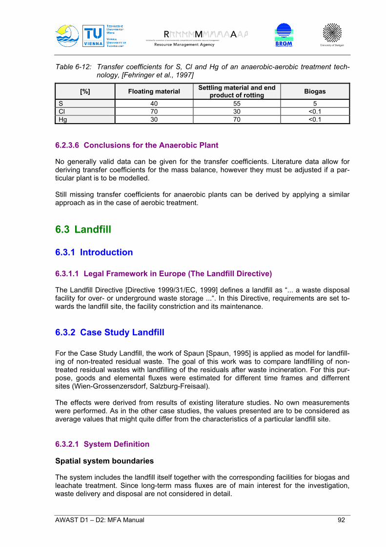
University of Stuttgart
AWAST D1 – D2: MFA Manual 92
Table 6-12: Transfer coefficients for S, Cl and Hg of an anaerobic-aerobic treatment tech-nology, [Fehringer et al., 1997]
[%] Floating material Settling material and end product of rotting Biogas
S 40 55 5 Cl 70 30 <0.1 Hg 30 70 <0.1
6.2.3.6 Conclusions for the Anaerobic Plant
No generally valid data can be given for the transfer coefficients. Literature data allow for deriving transfer coefficients for the mass balance, however they must be adjusted if a par-ticular plant is to be modelled. Still missing transfer coefficients for anaerobic plants can be derived by applying a similar approach as in the case of aerobic treatment. 6.3 Landfill
6.3.1 Introduction
6.3.1.1 Legal Framework in Europe (The Landfill Directive)
The Landfill Directive [Directive 1999/31/EC, 1999] defines a landfill as “... a waste disposal facility for over- or underground waste storage ...“. In this Directive, requirements are set to-wards the landfill site, the facility constriction and its maintenance. 6.3.2 Case Study Landfill
For the Case Study Landfill, the work of Spaun [Spaun, 1995] is applied as model for landfill-ing of non-treated residual waste. The goal of this work was to compare landfilling of non-treated residual wastes with landfilling of the residuals after waste incineration. For this pur-pose, goods and elemental fluxes were estimated for different time frames and differrent sites (Wien-Grossenzersdorf, Salzburg-Freisaal). The effects were derived from results of existing literature studies. No own measurements were performed. As in the other case studies, the values presented are to be considered as average values that might quite differ from the characteristics of a particular landfill site. 6.3.2.1 System Definition
Spatial system boundaries
The system includes the landfill itself together with the corresponding facilities for biogas and leachate treatment. Since long-term mass fluxes are of main interest for the investigation, waste delivery and disposal are not considered in detail.
University of Stuttgart
AWAST D1 – D2: MFA Manual 93
Time system boundaries
Time boundaries are set at 30, 100 and 1000 years, so as to enable the derivation of short-, middle- and long-term effects. Process selection for the system
Within the selected system, the processes Landfill, Leachate Treatment and Biogas Utilisa-tion are considered. For the purposes of elaborating a more detailed water balance, the process Landfill is subdivided into Landfill Surface and Landfill Body. Goods and element selection for the system
Environmental processes are disposed out of the system boundary. Import fluxes: Residual wastes, precipitation, air (for biogas utilisation), chemicals (for leachate treatment) Export fluxes: Evapotranspiration, surface flow off, treated off-gas, leachate treatment residuals (leachate from the biogas utilisation), lost biogas, wastewater, leachate treatment residuals (landfill leachate, process leachate treatment). Fluxes among the processes (input respectively output fluxes): Infiltration water, collected landfill gas, leachate As elements of relevance for the current study, carbon (C), nitrogen (N), phosphorus (P), sulphur (S), chlorine (Cl), iron (Fe), zinc (Zn), lead (Pb), cadmium (Cd), copper (Cu) and mercury (Hg) are selected. These elements are selected for their presenting matrix or trace elements to be detected in the environment or for their importance as raw materials (e.g. P, N as nutrients; Fe, Zn as technical raw materials). Further, the selected indicator elements prove certain chemical and physical characteristics that are crucial for their behaviour under given processes. This en-ables also an evaluation of the distribution of other elements of similar chemical behaviour within the processes considered. So for instance, elements like antimony, zinc or thallium show behaviour similar to cadmium when incinerated. Cobalt, manganese and chrome are comparable with iron as a lithophilic metal towards their chemical-physical behaviour [Baccini & Brunner, 1991]. Carbon is a main component of biogenous goods, a main carrier of chemical energy, and a basic element of toxic substances. Nitrogen is, as NO3, an essential nutrient; as NO2 and NOx a potential air pollutant. Phosphorus is, as phosphate, an essential nutrient and in natural water – a limiting nutrient. A lithophilic element. Sulphur is also an essential nutrient and, when incinerated, builds light volatile oxides. Chlorine builds as chloride light soluble salts. Together with other organic components, it can build very stable and very toxic compounds (e.g. PCB, Dioxins, Furans).

University of Stuttgart
AWAST D1 – D2: MFA Manual 94
Iron occurs as metal as part of a variety of consumption goods. Iron is a typical litophilic ele-ment as for its physical and chemical behaviour. Zinc is applied as corrosion protector, in batteries and as additive for gum. Lead builds as lead(II)-ion very stable complexes with organic ligands. Cadmium is as additive in a variety of consumption goods. Cadmium is a toxic heavy metal. Its chemical and physical behaviour proves its being a typical athmophilic (=light volatile) element. Copper builds, as Cu2+, very stable complexes with organic ligands. When solved, even very low copper concentrations are toxic for certain organisms. Mercury is, as cadmium, a typical athmophilic element (boiling point at 357°C). Under reduc-tive conditions, it builds metal-organic and toxic compounds [Baccini & Brunner, 1991].
Precipitation
Landfill surface
Infiltration water
Evapotranspiration
Biogas (collected)
Air
Residual wastes
Chemicals
LeachateLandfill body
Reservoir
Bio-chemical
degradation
Biogas utilisation
Leachate treatment
Surface flow-off
Treated gas
Residuals from biogas utilisation
Biogas (losses)
Wastewater
Residuals from leachate treatment
System boundary Landfill
Figure 6-10: System definition of a landfill for non-treated residual waste [Spaun, 1995]
6.3.2.2 Estimation of the goods and elemental fluxes
Composition of residual waste
The average values presented in Table 6-13 are elaborated by comparing the results of five studies on the elemental composition of residual waste. The water content is assumed as 30%mass of the moist solids weight.
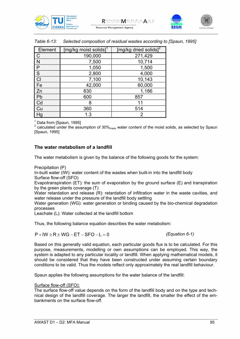
University of Stuttgart
AWAST D1 – D2: MFA Manual 95
Table 6-13: Selected composition of residual wastes according to [Spaun, 1995]
Element [mg/kg moist solids]1 [mg/kg dried solids]2
C 190,000 271,429 N 7,500 10,714 P 1,050 1,500 S 2,800 4,000 Cl 7,100 10,143 Fe 42,000 60,000 Zn 830 1,186 Pb 600 857 Cd 8 11 Cu 360 514 Hg 1.3 2
1 Data from [Spaun, 1995] 2 calculated under the assumption of 30%mass water content of the moist solids, as selected by Spaun [Spaun, 1995] The water metabolism of a landfill
The water metabolism is given by the balance of the following goods for the system: Precipitation (P) In-built water (IW): water content of the wastes when built-in into the landfill body Surface flow-off (SFO) Evapotranspiration (ET): the sum of evaporation by the ground surface (E) and transpiration by the green plants coverage (T) Water retardation and release (R): retardation of infiltration water in the waste cavities, and water release under the pressure of the landfill body settling Water generation (WG): water generation or binding caused by the bio-chemical degradation processes Leachate (L): Water collected at the landfill bottom Thus, the following balance equation describes the water metabolism:
0LSFOETWGRIWP =−−−±±+ (Equation 6-1) Based on this generally valid equation, each particular goods flux is to be calculated. For this purpose, measurements, modelling or own assumptions can be employed. This way, the system is adapted to any particular locality or landfill. When applying mathematical models, it should be considered that they have been constructed under assuming certain boundary conditions to be valid. Thus the models reflect only approximately the real landfill behaviour. Spaun applies the following assumptions for the water balance of the landfill: Surface flow-off (SFO): The surface flow-off value depends on the form of the landfill body and on the type and tech-nical design of the landfill coverage. The larger the landfill, the smaller the effect of the em-bankments on the surface flow-off.
University of Stuttgart
AWAST D1 – D2: MFA Manual 96
Since the assumption considers a large landfill with a plane surface, the surface flow-off is set equal to 0 (SFO=0). Precipitation (P): Precipitation is a crucial value for constructing the water balance. This value is to be esti-mated only by means of measuring. As annual precipitation amount, the average value for five years is assumed. Evapotranspiration (ET): Evapotranspiration is a function of climate conditions, type and structure of the landfill cover-age and on the water and nutrient supply of the green plants on it. A variety of approaches aims at estimating its value by employing empirical or physical methods. As examples, the formula of Haude and the combination equation of Penman are shown. Coming from these basic approaches, a number of their adaptations and modifications exist. After the precipitation value, the evapotranspiration significantly affects the water balance of a landfill. This is in particular valid for sites characterised by low precipitation, i.e. large amounts of water underlie evapotranspiration. For the site of Vienna (annual precipitation of 555 mm) it is calculated that 68 % - 85 % of the precipitation leaves the landfill through evapotranspiration. Water retardation (R): The composition of the wastes stored in the landfill body, the construction and the coverage types, the manner of waste in-building, the changes of the retardation characteristics of the landfill body by biochemical degradation processes and generated gas bubbles are all pa-rameters that determine the amount of retarded water. Settlement effects and biochemical degradation of organic substance lower the accumulation capacity of the landfill filling and thus water is set free. For freshly disposed wastes, the accumulation capacity is assumed to be exhausted at a water content of 40 % of the moist solids weight. Water generation (WG): Mainly anaerobic degradation processes take place in the landfill body, but also aerobic ones are present. The pure anaerobic degradation consumes 0.57 g water/ g degraded carbon. Aerobic degradation generates 1.21 g water / g degraded carbon. Generated and consumed water amount was for both considered landfill sites (Vienna, Salz-burg) so low that it could be neglected. Water metabolism modelling Mathematical models aiming at estimating the water balance of landfills consider in a differ-ent magnitude the effect of the parameters given in (Equation 6-1. For the practical applica-tion thus those models should be taken into account that best suit the particular landfill. For the estimation of the water balance, the method of Spillmann [Spillmann, 1988] and the mathematical model HELP were applied. The results show that leachate generation rises after the accumulation capacity is exhausted. From this moment on, the leachate amount approximately corresponds to the difference between precipitation and evapotranspiration amounts. Prior to this, the leachate amount is smaller. The moment of exhaustion of the ac-cumulation capacity is, as the leachate amount itself as well, also a function of the climate characteristics of the site and of the type of the landfill coverage.

University of Stuttgart
AWAST D1 – D2: MFA Manual 97
Estimation of the biogas amount
The anaerobic microbiological degradation of organic matter in the landfill body results in generation of biogas (landfill gas) consisting mainly of CO2 and CH4. The biogas consists of ca. 40 – 65 %vol CH4. The rest presents CO2 and small amounts of trace compounds (mainly H2S, carbohydrates and their compounds). Estimating the maximal possible biogas yield is relatively simple to achieve by considering the contents of biologically degradable carbon. It is more difficult to predict the time progress of the biogas production. Since a biological process is concerned, an entire set of parame-ters exists that effect it, e.g. temperature, moisture, density of the landfill coverage, waste composition. Lab experiments and on-site measurements have resulted in developing a vari-ety of mathematical models describing the behaviour of biogas production. In Spaun [Spaun, 1995], the model of Ehrig is selected. It describes the progress of biogas generation by applying two exponential functions. The first function considers a quick expo-nential raise until a maximal gas production rate is achieved (18 Nm3/t.a) within the first two years. This maximum is followed by a slow exponential abatement. In the 20th year, the bio-gas curve has sunk down to 2 Nm3/t.a. Estimating short-term elemental fluxes by the goods fluxes
Elemental fluxes over the leachate Multiplying the leachate flux with the elemental concentration gives the particular elemental flux. The concentration behaviour was analysed by evaluating the measurement results from differently old landfills (1, 5, 7, 10 years) [Baccini et al., 1987]. For the period of 10 to 20 years, constant concentrations were assumed, except for carbon. The carbon concentration sank from 1,900 mg/l down to 750 mg/l. Elemental fluxes over the biogas The elemental flux over the biogas was estimated in analogy to the freights over the leachate. Here, measurement values of [Baccini et al., 1987] were applied. as well The car-bon concentration for the period between 10 and 20 years was assumed constant. Estimating long-term elemental fluxes by the goods fluxes
For estimating the elemental fluxes in the period between 20 and 1000 years after the waste in-building, the approach by Belevi [Belevi & Baccini, 1989] was applied. Since the biogas production is no more of relevance, the element discharge over the leachate is only consid-ered. In the model of Belevi [Belevi & Baccini, 1989], the element concentrations are assumed to exponentially decrease in time. The magnitude of decrease is estimated by the current con-centration in the leachate and the still available and mobile amount of the given element in the landfill body at the end of the intensive reactor phase (20 years). 6.3.2.3 Results
In the study of Spaun [Spaun et al., 1994], it is shown that during the reactor phase of a land-fill for non-treated residual wastes, 25 % - 30 % of the carbon are carried out by the biogas.

University of Stuttgart
AWAST D1 – D2: MFA Manual 98
Approximately 8 % of the chlorine and 7 % of the nitrogen are discharged over the leachate. After 20 years, 99,9 % of the metals and, except for the carbon, 90 % of the non-metals (as average) are still remaining in the landfill body. A long-term consideration shows that the leachate concentrations of chlorine, phosphorus and organic carbon require the leachate to be treated for centuries to millennia. The duration of this after-care phase is crucially dependent on the precipitation at the particular landfill site.
University of Stuttgart
AWAST D1 – D2: MFA Manual 99
7 Literature
ADEME (1993) MODECOM - A Method for Characterization of household Waste. Basic manual. ADEME. Angers.
ADEME (1997) MODECOM - A Method for Characterization of household Waste. Methodo-
logical extra (2nd edition). ADEME. Angers. Ayres, R. U. (1989) Industrial Metabolism: Technology and Environment. Washington D.C.
National Academy Press. p. 23-49. Ayres, R. U.; Ayres, L. W.; McCurley, J.; Small, M. J.; Tarr, J. A.; Widgery, R. C. (1985) A
Historical Reconstruction of Major Pollutant Levels in the Hudson-Raritan Basin 1880-1980. Variflex Corporation.
Ayres, R. U.; Kneese, A. V. (1969) Pollution and environmental quality. In: The Quality of the
Urban Environment. Essays on "New Ressources" in an Urban Age. Hrsg. von H. S. Perloff. Washington D.C. Resources for the Future.
Baccini, P.; Bächler, M.; Brunner, P. H.; Henseler, G. (1985) Von der Entsorgung zum Stoff-
haushalt: Die Steuerung anthropogener Stoffflüsse als interdisziplinäre Aufgabe (From waste disposal to material management: the control of anthropogenic material fluxes as an interdisciplinary challenge). Müll und Abfall 17 (4). p. 99-108.
Baccini, P.; Bader, H.-P. (1996) Regionaler Stoffhaushalt. Erfassung, Bewertung und Steue-
rung. Spektrum Akademischer Verlag. Heidelberg, Berlin, Oxford. Baccini, P.; Brunner, P. H. (1991) Metabolism of the Anthroposphere. Springer-Verlag. Ber-
lin, New York. Baccini, P.; Daxbeck, H.; Glenck, E.; Henseler, G. (1993) METAPOLIS. Güterumsatz und
Stoffwechselprozesse in den Privathaushalten einer Stadt. 34A. Nationales For-schungsprogramm 25 "Stadt und Verkehr". ETH-Zürich. Eidg. Anstalt für Wasserver-sorgung, Abwasserreinigung und Gewässerschutz (EAWAG). Abteilung Abfallwirt-schaft und Stoffhaushalt. Zürich.
Baccini, P.; Henseler, G.; Figi, R.; Belevi, H. (1987) Water and Element Balances of Munici-
pal Solid Waste Landfills. Waste Management and Research 5 p. 483-499. Bailey, J. E. (1991) Towards a science of metabolic engineering. Science 252 p. 1668-1675. Belevi, H.; Baccini, P. (1989) Long-Term Behavior of Municipial Solid Waste Landfills. In:
Waste Management and Research. Jahrgang 7. Nummer 43-56. BGBl 164/1996 (1996) Verordnung des Bundesministers für Umwelt über die Ablagerung
von Abfällen (Deponieverordnung). BGBl 325/1990 (1990) Bundesgesetz über die Vermeidung und Behandlung von Abfällen
(Abfallwirtschaftsgesetz - AWG).

University of Stuttgart
AWAST D1 – D2: MFA Manual 100
Braun, R. (1998) Anaerobtechnologie für die mechanisch-biologische Vorbehandlung von Restmüll und Klärschlamm. 10/1998 Schriftenreihe des BMUJF. Bundesministeriums f. Umwelt, Jugend u. Familie. Wien.
Brunner, P. H.; Baccini, P.; Deistler, M.; Lahner, T.; Lohm, U.; Obernosterer, R.; Voet, E. v.
d. (1998) Materials Accounting as a Tool for Decision Making in Environmental Policy. Summary Report. (Projekt MAcTEmPo). Technische Universität Wien. Institut für Wassergüte und Abfallwirtschaft. Abteilung Abfallwirtschaft. Wien.
Brunner, P. H.; Daxbeck, H.; Henseler, G.; von Steiger, B.; Beer, B.; Piepke, G. (1990)
RESUB. Der Regionale Stoffhaushalt im Unteren Bünztal. Die Entwicklung einer Me-thodik zur Erfassung des regionalen Stoffhaushaltes. Eidg. Anstalt für Wasserversor-gung, Abwasserreinigung und Gewässerschutz. Abteilung Abfallwirtschaft und Stoff-haushalt. Dübendorf.
Brunner, P. H.; Daxbeck, H.; Obernosterer, R.; Schachermayer, E. (1994) Stoffbuchhaltung
Österreich - Vorprojekt. Technische Universität Wien, Institut für Wassergüte und Ab-fallwirtschaft, Abteilung Abfallwirtschaft. Wien.
Brunner, P. H.; Daxbeck, H.; Obernosterer, R.; Schachermayer, E. (1995) Machbarkeitsstu-
die Stoffbuchhaltung Österreich. 27 UBA-Berichte. Technische Universität Wien, Insti-tut für Wassergüte und Abfallwirtschaft, Abteilung Abfallwirtschaft. Wien.
Brunner, P. H.; Ernst, W. R. (1986) Alternative Methods for the Analysis of Municipal Solid
Waste. Waste Management & Research 4 (2). p. 147-160. Brunner, P. H.; Mönch, H. (1986) The flux of metals through municipal solid waste incinera-
tors. Waste Management & Research 4 (2). p. 105-119. Daxbeck, H.; Baumeler, A.; Merl, A.; Smutny, R.; Brunner, P. H. (1999) Grenzen der Erfas-
sung und Verwertung von Altpapier in Österreich. (Projekt GEVA). Technische Uni-versität Wien, Institut für Wassergüte und Abfallwirtschaft, Abteilung Abfallwirtschaft. Wien.
Daxbeck, H.; Brunner, P. H. (1993) Stoffflußanalysen als Grundlagen für effizienten Umwelt-
schutz. Oesterreichische Wasserwirtschaft 45 (3/4). p. 90-96. Daxbeck, H.; Lampert, C.; Morf, L.; Obernosterer, R.; Rechberger, H.; Reiner, I.; Brunner, P.
H. (1996) Der anthropogene Stoffhaushalt der Stadt Wien. (Projekt PILOT). Techni-sche Universität Wien. Institut für Wassergüte und Abfallwirtschaft. Abteilung Abfall-wirtschaft. Wien.
Daxbeck, H.; Schönbauer, A.; Brunner, P. H.; Maderner, W. (1997) Stoffbuchhaltung Öster-
reich - Zink. (Projekt Stobu - Zn). Technische Universität Wien, Institut für Wassergüte und Abfallwirtschaft, Abteilung Abfallwirtschaft. Wien.
Decision 96/350/EC (1996) Commission Decision adapting Annexes IIA and IIB to Council
Directive 75/442/EEC on waste. Directive 75/442/EEC (1975) Directive on waste. Directive 91/156/EEC (1991) Council Directive amending Directive 75/442/EEC on waste.

University of Stuttgart
AWAST D1 – D2: MFA Manual 101
Directive 94/62/EC (1994) Directive on packaging and packaging waste. Directive 1999/31/EC (1999) Directive on the landfill of waste. Directive 2000/76/EC (2000) Directive on the incineration of waste. Duvigneaud, P.; Denayeyer-De Smet, S. (1975) L'Écosystème Urbain Bruxellois. In: Produc-
tivité biologique en Belgique : SCOPE, Travaux de la Section Belge du Programme Biologique International. Hrsg. von P. Duvigneaud und Kestemont, P. Paris. Duculot. p. 581-597.
Eder, M.; Obernosterer, R.; Brunner, P. H.; Daxbeck, H.; Döberl, G.; Fehringer, R.; Huber,
R.; Lampert, C.; Rechberger, H.; Schachermayer, E. (2001) Untersuchungen über die Möglichkeiten der Ausrichtung der Abfallwirtschaft nach stofflichen Gesichtspunkten. (Projekt ABASG). 19/2001. Schriftenreihe des BMLFUW. Bundesministerium für Land- und Forstwirtschaft, Umwelt und Wasserwirtschaft. Wien.
Erlass NRW (DE) (2000) Arbeitshilfe Stoffflussanalyse bei abfallrechtlichen Beurteilungsfra-
gen des Ministeriums für Umwelt und Naturschutz, Landwirtschaft und Verbraucher-schutz des Landes Nordrhein-Westfalen.
Fehringer, R.; Rechberger, H.; Pesonen, H.-L.; Brunner, P. H. (1997) Auswirkungen unter-
schiedlicher Szenarien der thermischen Verwertung von Abfällen in Österreich (ASTRA). Technische Universität Wien, Institut für Wassergüte und Abfallwirtschaft, Abteilung Abfallwirtschaft. Wien.
Harant, M.; Nelles, M.; Hofer, M.; Lorber, K. E.; Raninger, B. (1999) Pilotprojekt zur mecha-
nisch-biologischen Restabfallbehandlung vor der Deponierung (MBRVD) im Mürzver-band - 2. Projektphase: Stoffstromanalyse. 15/1999 Schriftenreihe des BMUJF. Mon-tanuniversät Leoben, Institut für Entsorgungs- und Deponietechnik. Wien.
Hauer, W. (1999) Kontrolle der Restmengenziele von Abfällen an sonstigen Verpackungen
für das Kalenderjahr 1998. Auf österreichischen Deponien im Jahr 1998 abgelagerte Restmengen an sonstigen Verpackungen gemäß § 3(3) Verpackungsverordnung, BGBl. 649/1996. Technisches Büro Hauer. Korneuburg.
Ibrahim, H. A. (1998) Untersuchungen zu In- und Outputströmen bei der Restabfallvergärung
und Vergleich mit der Kompostierung. Diplomarbeit. Universität - Gesamthochschule Paderborn. Technischer Umweltschutz. Höxter.
INFRAS (1995) Stoffbilanz Vinylchlorid. 253. Schriftenreihe Umwelt. Umweltgefährdende
Stoffe. INFRAS. Bern. Jeneral, M. (1984) Angebots- und Nachfragestrukturen von Blei und Zink - Ansätze zur Er-
stellung von Rohstoffbilanzen in Österreich. Dissertation. Wirtschaftsuniversität Wien. Wien.
Kampel, E. (2002) Evaluation of computer assisted material flow models and application to
selected case studies. Masters Thesis. Vienna University of Technology. Institute for Water Quality and Waste Management. Group of Wastes and Resources Manage-ment. Wien.
University of Stuttgart
AWAST D1 – D2: MFA Manual 102
Keller, A.; von Steiger, B.; Schulin, R. (1999) Stoffflussanalyse als Vorsorgeinstrument im Bodenschutz: Eine Methode zur Quantifizierung der Unsicherheit von Stoffbilanzen landwirtschaftlicher Böden. Mitteilungen Deutsche Bodenkundliche Gesellschaft 91 p. 1478-1481.
Ketelsen, K.; Fehre, E.; Heckenkamp, G.; Lahl, U.; Zeschmar-Lahl, B.; Beckmann, M.; Wein-
eck, S.; Maselli, J.; Lemser, B. (1998) Möglichkeiten der Kombination von mecha-nisch-biologischer und thermischer Behandlung von Restabfällen - Abschlussbericht. 147 1114. Umweltbundesamt Berlin. Berlin.
Koca, D.; Nilsson-Djerf, J. (2000) Assessment of Different Methodologies/Studies Used to
Determine the Amount of Packaging Waste that Remains in Final Disposal - Experi-ences from Six European Countries. LUCAS (Lund University Center for Applied Sys-tem Dynamics). Lund.
Koch, M.; Plinke, E.; Oertlin, M. (1999) Dioxine und Furane. Stoffflussanalyse. 312. Schrif-
tenreihe Umwelt. Umweltgefährdende Stoffe. Prognos. Bern. Krammer, H.-J.; Domenig, M. (1995) Abfallaufkommen in Österreich: Materialien zum Bun-
desabfallwirtschaftsplan. 61, UBA Monographien. Umweltbundesamt Wien. Klagen-furt.
Lohm, U.; Anderberg, S.; Bergbäck, B. (1994) Industrial metabolism at the national level: A
case-study on chromium and lead pollution in Sweden, 1880-1980. In: Industrial me-tabolism: Restructuring for sustainable development. Hrsg. von R. U. Ayres und Si-monis, U. E. Tokyo. United Nations University Press. p. 376.
Major, R. H. (1938) Annals of Medical History X, New Series (5). S. 369-381. Merl, A. (1996) Vergleich der methodischen Ansätze von Stoffhaushaltsstudien. Diplomar-
beit. Technische Universität Wien. Institut für Wassergüte und Abfallwirtschaft. Abtei-lung Abfallwirtschaft. Wien.
Ministry of Housing Physical Planning and the Environment (1992) Natural Resources Ac-
counting: an aid to decision making in the context of policy on squandring. SP 1992/12. Paris.
Morf, L.; Ritter, E.; Brunner, P. H. (1997) Güter- und Stoffbilanz der MVA Wels. (Projekt
MAPE III). Technische Universität Wien, Institut für Wassergüte und Abfallwirtschaft, Abteilung Abfallwirtschaft. Wien.
Morf, L. S.; Brunner, P. H. (1998) The MSW Incinerator as a Monitoring Tool for Waste Man-
agement. Environmental Science & Technology 32 (12). p. 1812-1831. Mostbauer, P.; Schneider, M.; Angerer, T.; Binner, E.; Fuchs, A.; Konrad, W.; Lahl, U.; Lass-
nig, D.; Lechner, P.; Maurer, G.; Scharf, W.; Scheidl, K.; Widerin, M.; Zach, A.; Zeschmar-Lahl, B. (1998) Grundlagen für eine technische Anleitung zur mechanisch-biologischen Vorbehandlung von Abfällen. R-151, Reports. Umweltbundesamt Wien. Wien.
Newcombe, K., Kalma, I. D., Aston, A. R. (1978) The Metabolism of a City: The Case of
Hong Kong. Ambio: a journal of the human environment, research and management VII (1). p. 3-16.
University of Stuttgart
AWAST D1 – D2: MFA Manual 103
Obernosterer, R. (1994) Flüchtige Halogenkohlenwasserstoffe FCKW, CKW, Halone.
Stoffflußanalyse Österreich. Diplomarbeit. Technische Universität Wien. Institut für Wassergüte und Abfallwirtschaft. Abteilung Abfallwirtschaft. Wien.
ÖN EN ISO 14040 (1997) Umweltmanagement - Ökobilanz - Prinzipien und allgemeine An-
forderungen (ISO 14040:1997). Rechberger, H. (1999) Entwicklung einer Methode zur Bewertung von Stoffbilanzen in der
Abfallwirtschaft. Dissertation. Technische Universität Wien. Institut für Wassergüte und Abfallwirtschaft, Abteilung Abfallwirtschaft. Wien.
Schmidt-Bleek, F.; Behrensmeier, R. (1998) MAIA : Einführung in die Material-Intensitäts-
Analyse nach dem MIPS-Konzept. Wuppertal Texte. Birkhäuser. Berlin, Basel, Bos-ton.
Schmidt-Bleek, F.; Klüting, R. (1993) Wieviel Umwelt braucht der Mensch? MIPS: Das Maß
für ökologisches Wirtschaften. Birkhäuser. Berlin, Basel, Boston. Sievers, U. (1998) Ergebnisse des großtechnischen MBA-Pilotprojektes des Landkreis Ra-
vensburg. BMBF-Statusseminar Verbundvorhaben Mechanisch-biologische Behand-lung von zu deponierenden Abfällen. Potsdam.
Soyez, K., Hrsg. (2001) Mechanisch-biologische Abfallbehandlung: Technologien, Ablage-
rungsverhalten und Bewertung; Gesamtdarstellung der wissenschaftlichen Ergebnis-se des Verbundvorhabens "Mechanisch-biologische Behandlung von zu deponieren-den Abfällen". Abfallwirtschaft in Forschung und Praxis. Bd 120. Erich Schmidt Ver-lag. Berlin.
Spaun, S. (1995) Vergleich der Stoffbilanzen von Restmüllverbrennung und Restmülldepo-
nierung unter besonderer Berücksichtigung der Wasserbilanz. Diplomarbeit. Techni-sche Universität. Institut für Wassergüte und Abfallwirtschaft. Wien.
Spaun, S.; Schachermayer, E.; Kaas, T.; Lauber, W.; Brunner, P. H. (1994) Entscheidungs-
hilfen für die Verfahrensauswahl in der Abfallwirtschaft im Raum Oberöster-reich/Salzburg - Teil 1 Vergleich mechanisch-biologische Vorbehandlung und thermi-sche Behandlung. Technische Universität Wien, Institut für Wassergüte und Abfall-wirtschaft, Abteilung Abfallwirtschaft. Wien.
Spillmann, P. (1988) Wasserhaushalt von Abfalldeponien. Heft 3. TU Braunschweig, Zent-
rum für Abfallforschung. Sustain (1994) Forschungs- und Entwicklungsbedarf für den Übergang zu einer nachhaltigen
Wirtschaftsweise in Österreich. SUSTAIN - Verein zur Koordination von Forschung über Nachhaltigkeit. Graz.
United Nations (1974) Report of the Secretary General to the Statistical Commission, Statis-
tics of the Environment. E/CN.3/452. UN Document. New York. Vollmer, G.-R.; Meyer, A. (1998) Erschöpfende Vergärung von Restmüll mit Hygienisierung
und Schadstoffabbau. BMBF-Statusseminar Verbundvorhaben Mechanisch-biologische Behandlung von zu deponierenden Abfällen. Potsdam.
University of Stuttgart
AWAST D1 – D2: MFA Manual 104
Wolf, B.; Klonower, R. (2000) Regionale Material- und Energieflussrechnungen. In: Der Stoffhaushalt ländlicher Regionen: Analysen - Handlungsfelder - Perspektiven. Hrsg. von D. Thrän und Soyez, K. Potsdam Neuruppin. Universität Potsdam, Zentrum für Umweltwissenschaften. p. 14-24.
Zeschmar-Lahl, B.; Jager, J.; Ketelsen, K.; Lahl, U.; Scheidl, K.; Steiner, M.; Heckmann, A.
(2000) Mechanisch-Biologische Abfallbehandlung in Europa. Verband der Kommuna-len Abfallwirtschaft und Stadtreinigung e.V. (VKS) und Arbeitsgemeinschaft Stoffspe-zifische Abfallbehandlung (ASA). Parey Buchverlag. Berlin.