Embed Size (px)
Citation preview

University of Alberta
Axisymmetric Internal Solitary Waves Launched byRiver Plumes
by
Justine M. McMillan
A thesis submitted to the Faculty of Graduate Studies and Research in partial fulfillment of the
requirements for the degree of
Master of Science
Department of Physics
c©Justine M. McMillanSpring 2011
Edmonton, Alberta
Permission is hereby granted to the University of Alberta Libraries to reproduce single copies of this thesis
and to lend or sell such copies for private, scholarly or scientific research purposes only. Where the thesis is
converted to, or otherwise made available in digital form, the University of Alberta will advise potential
users of the thesis of these terms.
The author reserves all other publication and other rights in association with the copyright in the thesis
and, except as herein before provided, neither the thesis nor any substantial portion thereof may be printed
or otherwise reproduced in any material form whatsoever without the author’s prior written permission.

Examining Committee
Bruce Sutherland, Physics & Earth and Atmospheric Sciences
Martyn Unsworth, Physics & Earth and Atmospheric Sciences
Morris Flynn, Mechanical Engineering
Gordon Swaters, Mathematical and Statistical Sciences

Abstract
The generation and evolution of internal solitary waves by intrusive gravity
currents and river plumes are examined in an axisymmetric geometry by way
of theory, experiments and numerical simulations. Full depth lock-release ex-
periments and simulations demonstrate that vertically symmetric intrusions
propagating into a two-layer fluid with an interface of finite thickness can
launch a mode-2 double humped solitary wave. The wave then surrounds the
intrusion head and carries it outwards at a constant speed. The properties
of the wave’s speed and shape are shown to agree well with a Korteweg-de
Vries theory that is derived heuristically on the basis of energy conservation.
The numerical code is also adapted to oceanographic scales in an attempt
to simulate the interaction between the ocean and a river plume emanating
from the mouth of the Columbia River. Despite several approximations, the
fundamental dynamics of the wave generation process are captured by the
model.

Acknowledgements
This research would not have been possible without the support of my super-
visor, Dr. Bruce Sutherland. As well as being an ambitious scientist, Bruce
is a great mentor to all his students. I am particularly grateful for both the
challenges and opportunities that he has presented me with over the past two
years. The skills that I have developed as a result of these experiences will
enable me to be successful in whatever career path I choose.
I would also like to thank the members of my research group for their in-
sights and suggestions. In particular, I would like to acknowledge Amber, who
has been alongside me since day one. We engaged in many scientific, and non-
scientific, conversations that truly enriched my graduate student experience.
I am fortunate to have a family that provides me with unconditional love
and support. I would like to thank my parents for their encouragement and
my sisters for their friendship.
In addition, I am grateful to all the runners that I have met in Edmon-
ton. You allowed me to sustain the balance between life and school. The
engaging conversations during the 30+ km runs will become a blur, but the
companionship will never be forgotten.
I would like to acknowledge my committee members for their feedback
on my thesis, as well as their questions during my defense. Although the
evaluation was challenging, it was an invaluable learning experience. Finally,
I am grateful for the financial support of NSERC and the Alberta Ingenuity
Fund.

Table of Contents
1 Introduction 1
1.1 Motivation . . . . . . . . . . . . . . . . . . . . . . . . . . . . . 1
1.2 Background . . . . . . . . . . . . . . . . . . . . . . . . . . . . 3
1.2.1 Rectilinear Gravity Currents and Intrusions . . . . . . 3
1.2.2 Axisymmetric Gravity Currents . . . . . . . . . . . . . 4
1.2.3 Axisymmetric Solitary Waves . . . . . . . . . . . . . . 5
1.3 Thesis Overview . . . . . . . . . . . . . . . . . . . . . . . . . . 6
2 Theory 8
2.1 Rectilinear speed of a symmetric intrusion at a thick interface 9
2.2 Long small-amplitude waves at a thick interface . . . . . . . . 11
2.3 Internal Solitary Waves . . . . . . . . . . . . . . . . . . . . . . 15
2.3.1 Rectilinear KdV Theory . . . . . . . . . . . . . . . . . 16
2.3.2 Axisymmetric KdV – Rigorous Derivation . . . . . . . 17
2.3.3 Axisymmetric KdV – Heuristic Derivation . . . . . . . 20
3 Experiments 23
3.1 Set-up . . . . . . . . . . . . . . . . . . . . . . . . . . . . . . . 23
3.2 Analysis and Results . . . . . . . . . . . . . . . . . . . . . . . 24
3.3 Discussion . . . . . . . . . . . . . . . . . . . . . . . . . . . . . 25
4 Numerical Simulations 28
4.1 Governing Equations . . . . . . . . . . . . . . . . . . . . . . . 28

4.2 Solution Method . . . . . . . . . . . . . . . . . . . . . . . . . 30
4.3 Running the Code . . . . . . . . . . . . . . . . . . . . . . . . 32
5 Axisymmetric Vertically Symmetric Intrusions 35
5.1 Initial Conditions . . . . . . . . . . . . . . . . . . . . . . . . . 35
5.2 Results . . . . . . . . . . . . . . . . . . . . . . . . . . . . . . . 36
6 River Plumes 44
6.1 Columbia River Plume . . . . . . . . . . . . . . . . . . . . . . 45
6.2 Approximations and the Simulation Setup . . . . . . . . . . . 47
6.3 Analysis and Results . . . . . . . . . . . . . . . . . . . . . . . 52
6.4 Discussion . . . . . . . . . . . . . . . . . . . . . . . . . . . . . 60
7 Summary and Conclusions 65
List of Tables
4.1 Parameters for the numerical sponge layer . . . . . . . . . . . 33
6.1 Summary of river plume simulation measurements and Columbia
River observations . . . . . . . . . . . . . . . . . . . . . . . . 61

List of Figures
2.1 Schematic of mode-1 and mode-2 waves . . . . . . . . . . . . . 9
2.2 Schematic of a gravity current at a thick interface . . . . . . . 10
2.3 Relative intrusion and wave speeds as a function of interface
thickness . . . . . . . . . . . . . . . . . . . . . . . . . . . . . . 12
2.4 KdV parameters as a function of interface thickness . . . . . . 17
3.1 Schematic of experimental setup . . . . . . . . . . . . . . . . . 24
3.2 Snapshots and a time series from an intrusion experiment . . . 26
4.1 Schematic of the staggered grid used in numerical code . . . . 30
5.1 Position of the intrusion front versus time . . . . . . . . . . . 38
5.2 Snapshots from a simulation with δh = 0.2 . . . . . . . . . . . 39
5.3 Snapshots from a simulation with δh = 1.0 . . . . . . . . . . . 40
5.4 Wave amplitude versus position for δh = 0.2 . . . . . . . . . . 42
5.5 Solitary wave evolution and comparison to heuristic KdV theory
for δh = 0.2 . . . . . . . . . . . . . . . . . . . . . . . . . . . . 43
6.1 Progression of a plume emanating from the Columbia River . 46
6.2 In situ measurements of the Columbia River plume . . . . . . 48
6.3 Background density profiles for river plume simulations . . . . 50
6.4 Snapshots from a simulation with ρ = ρST and Hm
2= 50 m . . 53
6.5 Snapshots from a simulation with ρ = ρCR and Hm
2= 50 m . . 54
6.6 Richardson Number for Hm
2= 50 m . . . . . . . . . . . . . . . 55

6.7 Initial river plume speeds as a function of Hm
2. . . . . . . . . 56
6.8 Wave positions and speeds for ρ = ρST and Hm
2= 50 m . . . . 58
6.9 Wave amplitude as a function of radial position for ρ = ρST and
Hm
2= 50 m . . . . . . . . . . . . . . . . . . . . . . . . . . . . 59
Chapter 1
Introduction
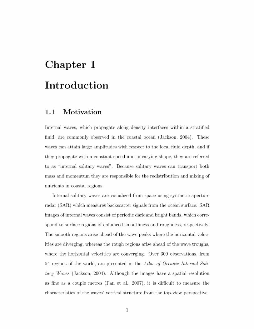
1.1 Motivation
Internal waves, which propagate along density interfaces within a stratified
fluid, are commonly observed in the coastal ocean (Jackson, 2004). These
waves can attain large amplitudes with respect to the local fluid depth, and if
they propagate with a constant speed and unvarying shape, they are referred
to as “internal solitary waves”. Because solitary waves can transport both
mass and momentum they are responsible for the redistribution and mixing of
nutrients in coastal regions.
Internal solitary waves are visualized from space using synthetic aperture
radar (SAR) which measures backscatter signals from the ocean surface. SAR
images of internal waves consist of periodic dark and bright bands, which corre-
spond to surface regions of enhanced smoothness and roughness, respectively.
The smooth regions arise ahead of the wave peaks where the horizontal veloc-
ities are diverging, whereas the rough regions arise ahead of the wave troughs,
where the horizontal velocities are converging. Over 300 observations, from
54 regions of the world, are presented in the Atlas of Oceanic Internal Soli-
tary Waves (Jackson, 2004). Although the images have a spatial resolution
as fine as a couple metres (Pan et al., 2007), it is difficult to measure the
characteristics of the waves’ vertical structure from the top-view perspective.
1
The advancement of ocean instrumentation, and specifically the develop-
ment of thermistor arrays, in the 1960s and 1970s motivated several observa-
tional in situ studies of internal solitary waves (Helfrich and Melville, 2006).
For example, waves were measured in the Andaman Sea (Perry and Schimke,
1965), the Strait of Gibraltar (Ziegenbein, 1969) and the Massachusetts Bay
(Halpern, 1971), among other locations. These, and related studies, demon-
strated that internal solitary waves can be generated by tidal currents flowing
over bottom topography, including shelf breaks and sills.
In the absence of topography, internal solitary waves can be launched by
gravity currents, which arise when a fluid of one density flows horizontally
into an ambient fluid of a different, or varying, density. In the ocean, these
currents may be manifest in the form of river plumes (Nash and Moum, 2005).
At high tide the ocean water forces the river water upstream. Then, as the
tide relaxes, ebb currents begin to flow allowing the fresh water from the river
to propagate along the surface of the coastal ocean. These plumes force the
denser near-surface ocean waters downwards launching an internal wave which
is manifest as an undulation of the pycnocline.
A distinguishing feature of SAR images of internal waves is that the fronts
tend to have some degree of curvature, regardless of whether the waves are
launched by localized topography or gravity currents. Most of the previous
experimental and theoretical attempts to characterize the dynamics of inter-
nal solitary waves have been limited to a rectilinear geometry which does not
describe the lateral spreading of the waves as they propagate away from their
source. The major thrust of this thesis is to extend earlier research into recti-
linear internal waves to the study of radially spreading internal waves.
2

1.2 Background
In this work, we focus on the generation of internal solitary waves from gravity
currents and “intrusions”, which are gravity currents that propagate at an
intermediate level between the upper and lower boundaries of a fluid along
their level of neutral buoyancy. We begin by reviewing existing experimental
and theoretical research on gravity currents and internal solitary waves in both
rectilinear and axisymmetric geometries.
1.2.1 Rectilinear Gravity Currents and Intrusions
Gravity currents are often studied in the laboratory by way of lock-release
experiments where two fluids of different densities are initially separated by
a vertical lock (e.g. see Simpson (1997)). The lock is then rapidly extracted
causing the denser fluid to flow beneath the lighter fluid. The propagation of
gravity currents can be divided into three distinct phases: the slumping phase,
the inertial (or self-similar) phase and the viscous phase. The slumping phase
occurs immediately after the lock removal and it is characterized by a gravity
current that moves at a constant velocity. In the inertial phase, the current
thins and decelerates, as the motion is dominated by buoyancy and inertial
forces. The viscous phase occurs when the motion is so slow and the current
is so thin that its evolution is dominated by the viscous and buoyancy forces
(Huppert, 1982).
Lock-release experiments of “symmetric” intrusions have been performed
in an approximate two-layer fluid with equal upper- and lower-layer depths
in which the intrusion density was the average ambient density (Britter and
Simpson, 1981; Faust and Plate, 1984; Rooij et al., 1999; Lowe et al., 2002). By
symmetry, such studies are equivalent to the examination of surface gravity
currents moving across a free-slip boundary in a stratified ambient. Unlike
3

gravity currents in uniform ambients, which are predicted to transition to the
inertial phase and decelerate after propagating 6 to 10 lock lengths (Rottman
and Simpson, 1983), symmetric intrusions at sufficiently thick interfaces were
found to propagate well beyond this distance at a constant speed (Mehta
et al., 2002; Sutherland and Nault, 2007). In a rectilinear geometry, intrusions
maintained a constant speed beyond 22 lock lengths. For small, but finite
interface thicknesses, the measured speed was faster than the linear long wave
speed, suggesting that the intrusion generated a solitary wave. Subsequently,
the closed-core solitary wave carried the intrusion outwards. The waves were
observed in intrusion experiments because the stratification at the interface
supported the formation of a wave. Similarly, if a surface gravity current
propagated into a thin stratified layer (the symmetric extension of a symmetric
intrusion at a thin interface), its speed was constant well beyond 10 lock lengths
(Sutherland and Nault, 2007).
1.2.2 Axisymmetric Gravity Currents
The dynamics of radially spreading gravity currents are qualitatively differ-
ent from rectilinear gravity currents because energy and mass conservation
require the head height to decrease. Hence the current should decelerate soon
after release due to the reduction of the horizontal pressure gradient driving
the flow. Lock-release experiments (Huppert and Simpson, 1980; Didden and
Maxworthy, 1982; Huq, 1996; Hallworth et al., 1996; Patterson et al., 2006)
demonstrated that axisymmetric bottom-propagating gravity currents main-
tain a constant speed up to 3 lock radii. Thereafter, in the inertial phase, the
position of the front changed as t1/2, consistent with the theory (Hoult, 1972;
Huppert and Simpson, 1980) that assumes the current maintains a self-similar
cylindrical shape. By symmetry, Zemach and Ungarish (2007) used shallow
water theory to extend this prediction to axisymmetric intrusion propagation,
4

again predicting that the intrusion decelerates shortly after release from the
lock.
Contrary to this prediction, full-depth lock release experiments demon-
strated that axisymmetric intrusions propagate at a constant speed well be-
yond 3 lock radii (Sutherland and Nault, 2007). This suggested that, as in
a rectilinear geometry, solitary waves were responsible for transporting the
lock-fluid long distances at a constant speed. The experiments thus put into
question the applicability of shallow water theory, which necessarily filters the
albeit weakly non-hydrostatic dynamics of solitary waves. However, the ex-
perimental analysis did not go on to study the wave generation and evolution
process.
Axisymmetric intrusions are symmetric expansions of the experiments by
Maxworthy (1980), who launched a solitary wave by releasing a bottom-
propagating gravity current into an ambient consisting of a shallow stratified
layer beneath a uniform density fluid. He observed that the front velocity of
the wave was nearly constant until its amplitude decreased beyond a critical
value. After this time the front position changed according to r ∼ t2/3.
In part of the work presented here, we will examine the advance of intru-
sions in different ambient densities. This will be done through the analysis of
experiments and numerical simulations.
1.2.3 Axisymmetric Solitary Waves
As explained in Section 1.1, the motivation for this work arises in part from
the observation of laterally spreading internal solitary waves, for which theory
is limited. In a rectilinear geometry, the weakly nonlinear Korteweg-de Vries
(KdV) model is appropriate if nonlinearity and nonhydrostatic dispersion are
comparable and small. Large amplitude closed-core solitary waves can be ac-
curately described by the fully nonlinear Dubreil-Jacotin-Long (DJL) equation
5
(Dubreil-Jacotin, 1937; Long, 1953, 1956).
Following up upon the work of Miles (1978), Weidman and Velarde (1992)
developed a theory for axisymmetric internal solitary waves within a strati-
fied ambient fluid. They predicted an amplitude dependence upon distance
as r−2/3. But, in an earlier paper, Weidman and Zakhem (1988) compared
this amplitude prediction with experiments by Maxworthy (1980) and found
that the amplitude differed by up to 34%. They explained that their weakly
nonlinear theory did not capture the experimental results because the trap-
ping of the mixed fluid was “a clear manifestation of strong nonlinear effects”.
They admitted, however, that their equation was asymptotically inconsistent
and so its predictions were not necessarily reliable. The theory presented by
Weidman and Velarde (1992) likewise relied upon inconsistent assumptions.
Part of the work presented here uses numerical simulations to examine
radially spreading solitary waves. From these observations, a heuristic theory
is developed to describe their evolution. Ultimately the goal of this thesis is to
provide some insight into the observed dynamics of solitary waves generated
by river plumes.
1.3 Thesis Overview
In this work we use theory, experiments and numerical simulations to charac-
terize the dynamics of internal solitary waves in an axisymmetric geometry1.
The thesis is organized such that the theory is summarized in Chapter 2, the
experiments are summarized in Chapter 3, and the numerical simulations are
summarized in Chapters 4–6.
More specifically, Chapter 2 outlines the theory governing the speed of a
vertically symmetric intrusion as a function of interface thickness. The theories
1Sections of Chapters 2 and 5 have been published: Justine M. McMillan and Bruce R.Sutherland (2010). Nonlinear Processes in Geophysics. 17: 443–453.
6

of axisymmetric linear waves and rectilinear solitary waves are then reviewed
before discussing two theories for cylindrical solitary waves. One theory was
derived rigorously using perturbation methods whereas the other was obtained
heuristically on the basis of an energy conservation assumption.
Chapter 3 discusses experiments of intrusions that were conducted in a
cylindrical tank. In the idealized setup, the intrusion was released from a
full-depth lock into an approximately two-layer ambient with equal upper-
and lower-layer depths. For all experiments, the density of the intrusion was
equivalent to the average density of the ambient fluid. The analysis methods
and results of measuring intrusion speeds are also provided in Chapter 3.
Chapter 4 describes the fully nonlinear numerical code that was used for
the simulation of axisymmetric internal waves. A discussion of how the code
was used to simulate intrusions is provided in Chapter 5, in which the results
are also compared to the idealized experiments of Chapter 3.
Chapter 6 explains how the code was used to simulate a river plume ema-
nating from the Columbia River and its consequent interaction with the ther-
mocline. The results of these simulations are then compared to the observa-
tions of Nash and Moum (2005).
Finally, in Chapter 7 a summary of the significant results of this work is
presented and directions for future work are suggested.
7

Chapter 2
Theory
This work involves the study of radially spreading intrusions and the interfa-
cial waves they generate. We begin by adapting existing theory for rectilinear
gravity currents in a uniform density fluid and in a uniformly stratified fluid
to develop a prediction for the speed of intrusions at interfaces of arbitrary
thickness. This analysis is restricted to the study of symmetric intrusions,
meaning that the density of the intrusion is the average ambient density and
the background density gradient is itself symmetric in the vertical. In Chap-
ters 3 and 5, we proceed to compare the speeds of experimental and simulated
radial intrusions with the rectilinear theory prediction. In doing so, we eval-
uate the effect of the initial curvature of the intrusion front upon setting the
radial intrusion speed.
Being symmetric, the intrusion most efficiently excites a mode-2 interfacial
wave, which bulges upwards above and downwards below the mid-depth of the
interface. These waves are sometimes referred to as being “varicose” because
of the double-humped shape of the isopyncals. A schematic comparing mode-1
and mode-2 waves is shown in FIgure 2.1. We briefly review the theory for
small-amplitude long interfacial waves with this mode-2 structure. Finally,
we review Korteweg-de Vries (KdV) theory for rectilinear solitary waves in
continuously stratified fluid. We then describe an adaptation of this theory
8

(a) (b)
Figure 2.1: Schematic showing the deflection of isopycnals for (a) mode-1 and(b) mode-2 waves in a vertically bounded domain.
for radially spreading solitary waves that is later compared to observations.
2.1 Rectilinear speed of a symmetric intrusion
at a thick interface
The speed of a rectilinear intrusion at an interface of finite thickness was first
predicted by Ungarish (2005) using a shallow water model. That said, his
result underpredicted the experimental speeds measured by Faust and Plate
(1984). These experiments were well described, however, by White and Hel-
frich (2008) who used a fully nonlinear Dubreil-Jacotin-Long (DJL) approach
to describe an intrusion at a finite-thickness interface. But that theory too is
limited because recent experiments and simulations by Bolster et al. (2008)
suggest that the theory of White and Helfrich (2008) overpredicts the intru-
sion speed for the limit of a linearly stratified ambient. In this limit, DJL
theory is obviously flawed because it unphysically requires the head height of
the intrusion to tend to zero.
Rather than adapt DJL theory, here we take the simplest approach to pre-
dict the rectilinear intrusion speed while ensuring that our result is in agree-
ment with the predictions for two-layer and linearly stratified ambients. The
9

ρi
hT
1
2hT h
2
1
2(hT−h)
ρU
ρi
Figure 2.2: The domain and the density profile used to derive a theory for thespeed of intrusions as a function of interface thickness.
background density profile, ρ, is assumed to have the piecewise-linear form,
ρ(z) =
ρU
h2< z < H
2
ρi + zh
(ρU − ρL) − h2≤ z ≤ h
2
ρL − H2< z < −h
2,
(2.1)
where h is the thickness of the interface and ρi = 12(ρU + ρL) is the average
of the upper and lower layer densities. To take advantage of symmetry, the
level z = 0 is positioned at the mid-depth of the fluid, which has a total depth
H. The intrusion can be viewed as a symmetric expansion of a surface- or
bottom-propagating gravity current within an ambient of total depth hT = H2
,
as illustrated in Figure 2.2.
We first formulate the speed of a gravity current with density ρi moving
in an ambient with density given by (2.1) for 0 ≤ z ≤ hT ≡ H2
. Benjamin
(1968) predicted that an energy conserving gravity current released from a
lock of height hT will propagate with a head height of hT/2 in a uniform
ambient. Ungarish (2006) made an equivalent prediction for the propagation
of a gravity current in a linearly stratified ambient. Here, it is also assumed
that the head height is hT/2 and thus the the mean density over the depth of
10

the bottom-propagating gravity current is given by
ρavg =
{ρU + (ρi − ρU)δh 0 ≤ δh ≤ 0.5ρi + ρU−ρi
4δh0.5 < δh ≤ 1,
(2.2)
where δh ≡ hH
. The gravity current speed, Ugc, given by Benjamin (1968) for
a one-layer fluid and by Ungarish (2006) for a linearly stratified fluid is
Ugc =1
2
√g
(ρi − ρavgρ00
)hT. (2.3)
Here we have used the Boussinesq approximation allowing us to normalize the
density difference by the characteristic density ρ00.
By extension, the speed Ui of an intrusion moving along the interface of a
stratified fluid with a density profile given by (2.1) is predicted by combining
(2.2) and (2.3) and letting hT = H/2 to give
Ui = U0
{(1− δh)1/2 0 ≤ δh ≤ 0.512δ−1/2h 0.5 < δh ≤ 1,
(2.4)
where U0 is the speed of a symmetric intrusion in a two-layer fluid (δh = 0),
given by
U0 =1
4
√g′LUH. (2.5)
Here the reduced gravity between the upper and lower ambient fluid is
g′LU = g
(ρL − ρU
ρ00
). (2.6)
As illustrated by the dashed line in Figure 2.3, the intrusion speed is pre-
dicted to decrease as the relative thickness of the interface, δh, increases. This
formula correctly predicts the rectilinear intrusion speed in the two-layer limit
(δh → 0) and in the uniformly stratified limit (δh → 1).
2.2 Long small-amplitude waves at a thick in-
terface
Symmetric intrusions may efficiently excite mode-2 solitary waves if they travel
faster than long mode-2 interfacial waves at a thick interface. Rectilinear intru-
11

0.0 0.2 0.4 0.6 0.8 1.0δh
0.0
0.2
0.4
0.6
0.8
1.0
Ui
U0
c0
U0
Figure 2.3: Relative initial intrusion speeds, Ui/U0, computed numerically forambients with piecewise-linear (squares) and hyperbolic tangent (triangles)profiles (discussed in Chapter 5) are compared to the predicted rectilinearspeed (dashed line) defined by (2.4) and the relative speed, c0/U0, of a mode-2linear long wave (solid line) defined by (2.20). Experimental speeds (discussedin Chapter 3) are plotted as circles with corresponding largest error bars shownin the lower right hand corner.
sion speeds were thus compared with long mode-2 waves in the x-z plane with a
piecewise-constant three-layer density profile (Mehta et al., 2002; Sutherland
and Nault, 2007). Here we find the speed of long axisymmetric interfacial
waves in a three-layer fluid with piecewise-linear background density given by
(2.1).
A cylindrical coordinate system is represented by a radial direction, r,
an azimuthal direction, θ, and a vertical direction, z. In an axisymmetric
system, derivatives with respect to θ are zero. Under this assumption, the
fully nonlinear equations of motion for an inviscid, incompressible, Boussinesq
12
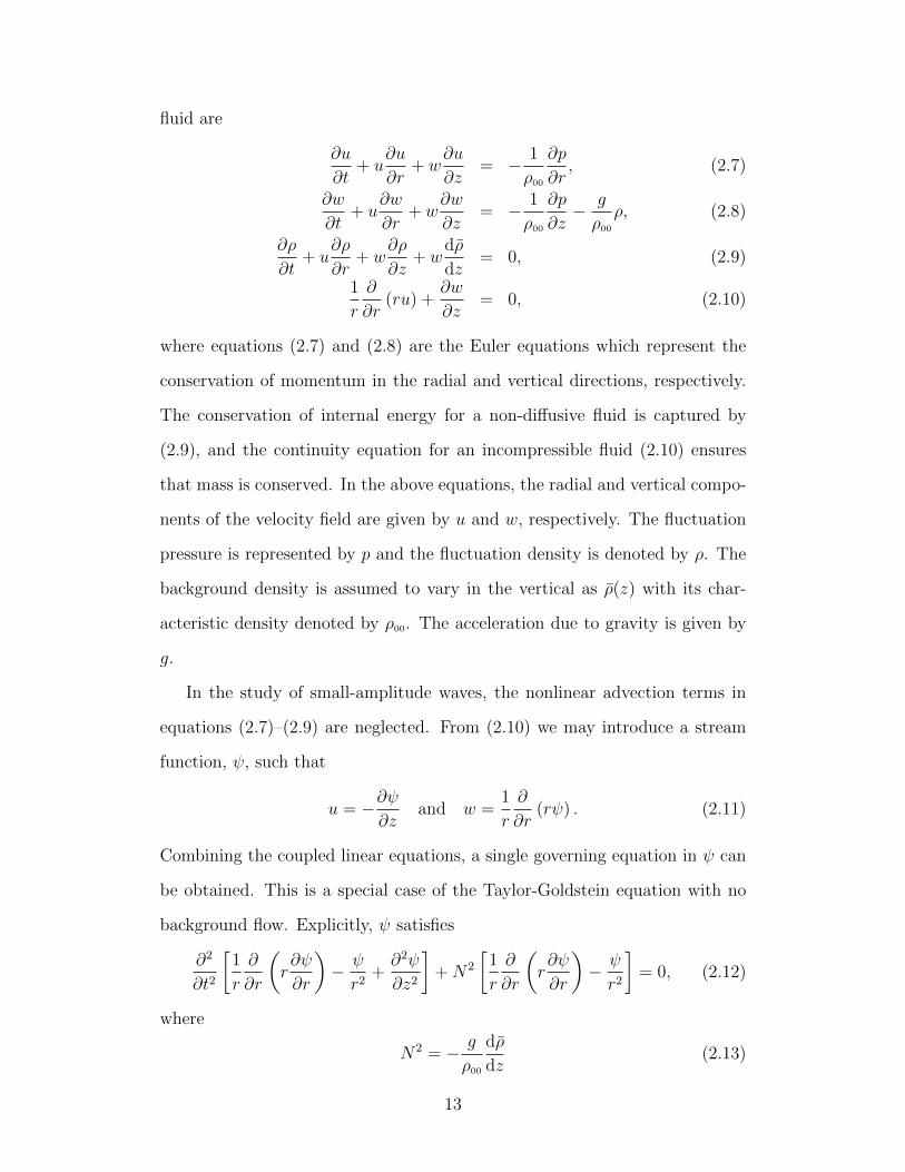
fluid are
∂u
∂t+ u
∂u
∂r+ w
∂u
∂z= − 1
ρ00
∂p
∂r, (2.7)
∂w
∂t+ u
∂w
∂r+ w
∂w
∂z= − 1
ρ00
∂p
∂z− g
ρ00
ρ, (2.8)
∂ρ
∂t+ u
∂ρ
∂r+ w
∂ρ
∂z+ w
dρ
dz= 0, (2.9)
1
r
∂
∂r(ru) +
∂w
∂z= 0, (2.10)
where equations (2.7) and (2.8) are the Euler equations which represent the
conservation of momentum in the radial and vertical directions, respectively.
The conservation of internal energy for a non-diffusive fluid is captured by
(2.9), and the continuity equation for an incompressible fluid (2.10) ensures
that mass is conserved. In the above equations, the radial and vertical compo-
nents of the velocity field are given by u and w, respectively. The fluctuation
pressure is represented by p and the fluctuation density is denoted by ρ. The
background density is assumed to vary in the vertical as ρ(z) with its char-
acteristic density denoted by ρ00. The acceleration due to gravity is given by
g.
In the study of small-amplitude waves, the nonlinear advection terms in
equations (2.7)–(2.9) are neglected. From (2.10) we may introduce a stream
function, ψ, such that
u = −∂ψ∂z
and w =1
r
∂
∂r(rψ) . (2.11)
Combining the coupled linear equations, a single governing equation in ψ can
be obtained. This is a special case of the Taylor-Goldstein equation with no
background flow. Explicitly, ψ satisfies
∂2
∂t2
[1
r
∂
∂r
(r∂ψ
∂r
)− ψ
r2+∂2ψ
∂z2
]+N2
[1
r
∂
∂r
(r∂ψ
∂r
)− ψ
r2
]= 0, (2.12)
where
N2 = − g
ρ00
dρ
dz(2.13)
13

is the squared buoyancy frequency.
Using separation of variables, (2.12) can be solved to give bounded solutions
of the streamfunction in the form
ψ(r, z, t) = AψJ1(kr)φ(z)e−iωt, (2.14)
where Aψ is the amplitude, k is the radial wavenumber, ω is the wave frequency,
J1 is the first-order Bessel function of the first kind and φ is the vertical
structure function which solves
d2φ
dz2+ k2
(N2
ω2− 1
)φ = 0. (2.15)
The solution of this ordinary differential equation depends on the upper and
lower boundary conditions as well as the stratification of the fluid prescribed
through N2.
In a fluid with a density profile given by (2.1) and no-normal-flow boundary
conditions at z = ±H2
, the vertical structure of a mode-2 wave satisfies
φ(z) =
sinh[k(H2−z)]
sinh[ k2 (H−h)]h2< z < H
2
sin (mz)
sin (mh2 )
− h2≤ z ≤ h
2
− sinh[k(H2
+z)]sinh[ k2 (H−h)]
− H2< z < −h
2.
(2.16)
Here the vertical wavenumber of the disturbance within the interface is
m = k√N2
0/ω2 − 1, (2.17)
in which the squared buoyancy frequency of the thick interface is
N20 =
g
ρ00
(ρL − ρU)
h. (2.18)
Using (2.17), k and ω are implicitly related by the dispersion relation
k tan
(mh
2
)+m tanh
[k
2(H − h)
]= 0. (2.19)
14

In the long wave limit this becomes
tan
(N0h
2c0
)+N0
2c0
(H − h) = 0, (2.20)
where c0 = ω/k is the long wave speed for a mode-2 wave. This speed is
plotted by the solid line in Figure 2.3. The same result would be found for
rectilinear interfacial waves. This indicates that although the radial structure
of the waves is different, the long wave speed is the same.
Given that the interface has a finite thickness (δh > 0), we expect that a
mode-2 wave can be established by the widening of the interface. Furthermore,
if the intrusion speed is supercritical (Ui > c0) we expect the wave to take the
form of a nonlinear solitary wave, whereas subcritical intrusions (Ui < c0)
generate linear waves. Whether, or not, the intrusion is supercritical can be
prescribed by the value of the Froude number, Fr ≡ Ui/c0. This is defined
such that Fr > 1 corresponds to a supercritical intrusion from which solitary
waves are expected to be generated. Comparing the solid and dashed lines in
Figure 2.3, we expect that Fr > 1 if δh > 0.5.
2.3 Internal Solitary Waves
KdV theory for rectilinear internal solitary waves is well-established (Benney,
1966). Using perturbation methods, Weidman and Velarde (1992) attempted
to extend the theory to an axisymmetric geometry. However, the result was
asymptotically inconsistent and it predicted an amplitude decrease as r−2/3,
inconsistent with energy conservation. Here, after reviewing rectilinear theory
we present two alternate approaches, one rigorous and one heuristic, that are
used to derive an energy conserving axisymmetric KdV equation.
15

2.3.1 Rectilinear KdV Theory
In a rectilinear geometry, internal solitary waves in a stratified fluid can be
modelled by the KdV equation. The formulation by Benney (1966) predicts
that in the Boussinesq approximation the vertical displacement field, ξ, has
the form
ξ(x, z, t) = a(x, t)φ(z), (2.21)
in which a(x, t) = a(x − ct) satisfies the KdV equation that includes the
advection term:
at + c0ax + γaax + βaxxx = 0. (2.22)
Here the subscripts denote derivatives and the constants γ and β are given by
(Benney, 1966)
γ =3
2c0
∫ H2
0φ3z dz∫ H
2
0φ2z dz
and β =1
2c0
∫ H2
0φ2 dz∫ H
2
0φ2z dz
, (2.23)
where c0 is the linear long wave speed. For a stratified ambient with the density
profile given by (2.1), we exploit symmetry and consider only the upper half
of the domain (hT = H2
). The corresponding vertical structure function, φ,
is given by the long wave limit of (2.16) with 0 ≤ z ≤ H2
and the long wave
speed, c0, satisfies (2.20).
The solution of (2.22), which assumes an isolated, steadily propagating
disturbance is
a(x− ct) = a0 sech2
(x− ctλ
). (2.24)
The speed, c, and width, λ, of the wave depend on the maximum displacement
amplitude, a0, by
c = c0 +γ
3a0 and λ2 =
12β
γ
1
a0
. (2.25)
The KdV coefficients, along with the wave speed and width, are shown in
Figure 2.4 as functions of interface thickness.
16

0.00 0.25 0.50δh
0
1
2
3
4
γ
a0
0.0
0.2
0.4
0.6
0.8
1.0
β
c0h2
(a)
0.00 0.25 0.50δh
0
1
2
3
4
cc0
0
1
2
3
λ
h
(b)
Figure 2.4: (a) Coefficients of the KdV equation as functions of interfacethickness. The nonlinear coefficient, γ, is shown by the solid line and thedispersion coefficient, β, is shown by the dashed line. (b) The speed, c, (solidline) and width, λ, (dashed line) of a rectilinear solitary wave as a function ofinterface thickness.
From the numerical simulations, which are reported upon later, it is easier
to diagnose the structure of the vertical velocity rather than the vertical dis-
placement field. The vertical velocity derived from the vertical displacement
field is
w(x, z, t) =∂ξ
∂t' 2.598Aw sech2
(x− ctλ
)tanh
(x− ctλ
)φ(z), (2.26)
in which the coefficient satisfies
2a0c
λ' 2.598Aw. (2.27)
Here Aw is defined as the maximum value of w. In these expressions, the value
2.598 is determined from the computed maximum value of sech2(x) tanh(x).
2.3.2 Axisymmetric KdV – Rigorous Derivation
Weidman and Velarde (1992) extended the theory of Benney (1966) to derive
a formula for the leading order weakly nonlinear evolution of axisymmetric
internal solitary waves. Here we outline a similar derivation but we further
17

impose that the amplitude of the wave must decrease as r−1/2 as is required
by energy conservation.
For an incompressible Boussinesq fluid, the governing equations of motion
are given by (2.7) – (2.10). Putting the nonlinear terms on the right-hand
side, the equations are
ρ00ut + pr = −ρ00(uur + wuz), (2.28)
pz + ρg = 0, (2.29)
ρt + wρ ′ = −(uρr + wρz), (2.30)
1
r(ru)r + wz = 0, (2.31)
in which the subscripts denote partial derivatives. Because we are interested
in long waves, it is assumed for now that the flow is hydrostatic. Therefore,
the vertical momentum equation (2.8) is replaced by (2.29). In Eulerian co-
ordinates, the vertical displacement field, ξ, is related at leading order to the
velocity fields by
w − ξt '1
r(rξu)r. (2.32)
The linear terms on the left-hand side of (2.28) – (2.32) can be combined to get
a linear operator acting on ξ alone. The corresponding right-hand side of the
resulting combined equation gives the nonlinear terms which non-negligibly
perturb the displacement of moderately large amplitude waves.
To determine the weakly nonlinear evolution equation, the vertical dis-
placement field is expanded in terms of the amplitude parameter, α, as follows:
ξ(r, z, t) = αξ0 + α2ξ1 + ... (2.33)
The vertical structure of the leading order solution, ξ0, is assumed to be sep-
arable from the slowly varying horizontal space and time dependence in the
following way:
ξ0 =(r0
r
)1/2
A(R, τ)φ(z). (2.34)
18

Here R = ε(r− ct) is the translating radial co-ordinate which varies slowly as
measured by ε. For consistency with the perturbation analysis that follows, the
slow time scale is taken to be τ = εαt. Different from the axisymmetric theory
of Weidman and Velarde (1992), here we have imposed energy conservation by
requiring the magnitude of ξ0 to decrease as r−1/2 beyond some radius r0. The
vertical structure function, φ, and the amplitude, A, are both of order unity.
Inserting (2.33) and the corresponding expansions for ~u, ρ and p into the
governing equations (2.28) – (2.32), extracting leading order terms in α, and
assuming r/r0 is large gives
Lξ0 = 0, (2.35)
where the linear operator L is defined as
L ≡ c20∂Rzz +N2∂R, (2.36)
in which N2(z) is the squared buoyancy frequency. Equations (2.35) and (2.36)
result in the ordinary differential equation for the vertical structure function
c20φ′′ +N2φ = 0. (2.37)
In particular, for the piecewise-linear density profile given by (2.1), φ is given
by the long-wave limit of (2.16); the vertical structure is the same whether in
a rectilinear or cylindrical geometry.
At order α2 and assuming r � r0, the following equation is satisfied:
Lξ1 = N , (2.38)
where the nonlinear operator N is given in terms of the leading-order functions
A and φ through
N = 2c0φ′′Aτ + [ 2c2
0(φφ ′)zz+2N2φφ ′′ + (N2)zφ2
+ 2c20φ′φ ′′ − c2
0(φφ′′)z ](r0
r
)1/2
AAR .(2.39)
Here the primes and z-subscripts both denote ordinary z-derivatives.
19

Recognizing (2.36) as a self-adjoint operator in z, both sides of (2.38) are
multiplied by ξ0 and the result is integrated over the domain height (0 ≤ z ≤
hT ). By construction, the left-hand side evaluates to zero, thus we arrive at the
following approximate equation describing the influence of nonlinearity upon
the amplitude A at large r >> r0:
Aτ + γ(r0
r
)1/2
AAR = 0. (2.40)
Additionally including the effects of linear dispersion introduces the term
βARRR on the left-hand side of (2.40). In the result, both γ and β are defined
as for rectilinear waves by (2.23). The result can rewritten in terms of r, t and
a = α(r0r
)1/2A, as
at + c0
(ar +
a
2r
)+ γ
(aar +
a2
2r
)+ βarrr = 0. (2.41)
Somewhat surprisingly, with the omission of the a2/2r term, this result is
identical to that of Weidman and Velarde (1992). Furthermore, setting φ(z) to
be the vertical structure function of surface waves in a one-layer fluid gives the
formula derived by Miles (1978) for cylindrical solitary surface waves. How-
ever, as was pointed out by Weidman and Zakhem (1988) for the surface wave
equation, the theory presented here is asymptotically inconsistent. By requir-
ing r � r0 in order to arrive at the KdV-like equation (2.41), the balance
between nonlinear steepening and dispersion may no longer be valid. Fur-
thermore, Weidman and Zakhem (1988) found that for large r, the solution
of (2.41) satisfied a ∼ r−2/3, whereas energy conservation requires that the
amplitude decreases with radius as r−1/2.
2.3.3 Axisymmetric KdV – Heuristic Derivation
Because the rigorous attempt at deriving an axisymmetric KdV equation did
not yield an energy conserving result, here we attempt to extend the rectilinear
20

theory to describe a solitary wave that spreads radially. For a solitary wave
spreading as an expanding ring with sufficiently large radius, we may assume
that the front on any point along the circumference negligibly feels the curva-
ture of the front but that the amplitude nonetheless decreases with radius as
r−1/2. Thus, by extension of (2.26), we predict that the vertical velocity field
should evolve as
w ' 2.598Aw0
(r0
r
)1/2
sech2
(r − ctλ
)tanh
(r − ctλ
)φ(z), (2.42)
in which the amplitude Aw0 is measured at a distance r0 where the axisym-
metric solitary wave is first generated.
For measured Aw0, we can use (2.25) and (2.27) to determine the initial
displacement amplitude, a0, the solitary wave speed, c, and the width, λ. As
the wave spreads radially, Aw = Aw0(r0/r)1/2 decreases. Correspondingly,
these equations predict that the displacement amplitude and speed should
decrease and its width should increase. Eventually, the amplitude will be
so small that weakly nonlinear effects associated with wave steepening will
become negligible, so that linear dispersion dominates the evolution.
In contrast to the asymptotically inconsistent equation (2.41), the heuristic
solution of the form (2.42) is established for r & r0. The corresponding vertical
displacement field of the form a(r, t) = a0(r0/r)1/2sech2[(r − ct)/λ] does not
satisfy (2.41). Instead, through manipulation of rectilinear KdV theory, it
satisfies the leading-order equation
at + c0
(ar +
a
2r
)+ γ
(r
r0
)1/2 [aar +
a2
2r
]+ βarrr = 0. (2.43)
Compared to (2.41), here the nonlinear term is of order (r/r0)1/2, which seems
to suggest that the balance between nonlinearity and dispersion exists for large
r. However, because a ∝ r−1/2 the nonlinear term will eventually become
negligible as the wave moves to large r and the motion will then be governed
21

by
at + c0
(ar +
a
2r
)+ βarrr = 0. (2.44)
This equation simply describes a dispersing linear wave. Using the method of
stationary phase, it can be shown that the dispersion results in spreading such
that the amplitude decreases as r−1/2. Together with the effect of geometrical
spreading, the amplitude of a long wave thus decreases as r−1.
Through comparison of these theories with the results of numerical simu-
lations (Chapter 5), we will show that the heuristic solution (2.42) more ac-
curately represents the life-cycle of axisymmetric solitary waves generated by
intrusions. Thus we show that the admittedly inconsistently derived cylindri-
cal solitary wave equation of Weidman and Velarde (1992) and our extension
of it in Section 2.3.2, indeed provide an inaccurate description of axisymmet-
ric solitary waves. However it must be emphasized that (2.43) is heuristic:
whereas the balance in rectilinear KdV theory for a disturbance of length L
is aL2 ∼ 1, the nonlinear dispersive ‘balance’ is aL2 ∼ r−1/2. And so the na-
ture of competition between nonlinearity and dispersion changes with radial
distance.
22

Chapter 3
Experiments
The motivation for this work was largely based on the experiments of axisym-
metric intrusions that were conducted, but not analysed, by Joshua Nault
and Lauren Blackburn in 2003 and 2004, respectively. I did conduct some
experiments myself, although the results are not presented here. This chapter
reports primarily upon the analysis methodology and the quantitative results.
3.1 Set-up
Experiments were conducted in a cylindrical acrylic tank with an inner di-
ameter of 2R = 90.7 cm and a height of 30.0 cm as illustrated in Figure 3.1.
The tank was filled to a depth of 5 cm with salt water of density ρL. Using a
sponge float, fresh water of density ρU was added to the surface until the total
depth of the fluid was H = 10 cm. In all experiments, the density of the upper
layer was ρU = 0.9982 g/cm3, whereas the lower layer density varied between
ρL = 1.0515 g/cm3 and ρL = 1.1047 g/cm3. Due to mixing and diffusion dur-
ing the filling process, the interface between the two layers was assumed to
vary smoothly over a depth of h = 1.5± 0.5 cm.
A small acrylic cylindrical lock with an inner diameter of 2r0 = 12 cm and
a height of 22.8 cm was inserted at the centre of the tank. The fluid within the
lock was then dyed and vigorously mixed, so that its density, ρi, was equal to
23

2R
2r0
ρL
ρU
ρi
H
2
H
2
H
Figure 3.1: A side-view schematic of the experimental setup used to observeintrusions propagating in a cylindrical tank. Although the ambient fluid isshown here as two distinct layers, it was assumed that the filling process anddiffusion caused the interface to have a thickness of approximately 1.5±0.5 cm.For all experiments, the density of the fluid within the lock was ρi = 1
2(ρU+ρL).
the mean density of the ambient fluid. The small concentration of dye allowed
the intrusion to be visualized without significantly changing the density of the
fluid in the lock.
Using a string and pulley system, the cylindrical lock was rapidly lifted
vertically out of the tank. This caused an intrusion to propagate outwards
along the interface between the light and dense fluid. An experiment was con-
sidered successful if the lock removal was purely vertical causing the intrusion
to propagate axisymmetrically.
3.2 Analysis and Results
Figures 3.2(a) and (b) show an overhead view taken from a COHU CCD
camera situated 2 m above the tank. These snapshots were taken at t = 2 s and
4 s after the lock was removed. The circular spreading of dyed fluid indicates
that the intrusion propagates axisymmetrically and the linear diagonal contour
in the time series (Figure 3.2c) confirms that it does so at a constant rate. At
about t = 6 s, the intrusion reflects off the cylinder side wall at R ' 45 cm
24

and then returns to the centre of the tank at approximately the same speed.
The magnitude of the speed was determined by measuring the slopes of two
diagonal contours from time series images. These measurements were typically
made between r = 12 cm and r = 24 cm (i.e. between one to three lock-radii
from the edge of the lock). The intrusion speed, Ui, was then calculated as
the average of the four slope values. The experimental error was taken to be
the standard deviation in the slopes.
3.3 Discussion
The measured speeds in six experiments are plotted as solid circles in Fig-
ure 2.3. In the figure, the speeds are non-dimensionalised by U0, given by (2.5).
For all experiments, the interface thickness was taken to be h = 1.5(±0.5) cm;
therefore, with H = 10 cm, δh = 0.15(±0.05). With the exception of one
experiment, Figure 2.3 shows that within error the measured speeds collapse
to a value of 0.75(±0.06)U0. This suggests that axisymmetric intrusions are
slower than rectilinear intrusions which, for δh = 0.15, have a predicted speed
of Ui/U0 ≈ 0.92 by (2.4). Furthermore, the measurements are consistent with
axisymmetric gravity current experiments (Huppert and Simpson, 1980; Pat-
terson et al., 2006) and simulations (Zhang et al., 2010), in which the observed
front speeds were about 0.8Ugc. Here Ugc, given by (2.3), plays the role of U0
for gravity currents.
The experiments that are presented here were all vertically symmetric,
meaning that the depths of the upper and lower layers were equal and the
density of the intruding fluid was equal to the average density of the ambient
(ie. ρi = 12
(ρU + ρL)). In all six experiments, the intrusions propagated
to the tank wall at a constant speed, a distance of 6.5r0 from the edge of
the lock. As explained in Section 1.2.2, axisymmetric gravity currents are
expected to decelerate around 3r0 from the release location, a consequence
25

-30
-15
0
15
30
y (c
m)
(a) t=2 s
-30 -15 0 15 30x (cm)
-30
-15
0
15
30
y (c
m)
(b) t=4 s
-40 -20 0 20 40r (cm)
0
5
10
15
20
25
t (s
)
(c)
Figure 3.2: Top view images at (a) t = 2 s and (b) t = 4 s. (c) Timeseries of an axisymmetric intrusion where the ambient density difference isρL − ρU = 0.1065 g/cm3. The lock fluid is darkly dyed. The diamond pat-tern in the time series indicates that the intrusion moves at a constant speedradially away from the lock and also radially inward after reflection from theside walls.
26

of their decreasing head height, but this does not happen in the vertically
symmetric intrusion experiments. Instead they propagate at a constant speed
beyond 8 lock radii. It is therefore hypothesized that the vertical symmetry
of the experiments presented here allows the intrusion efficiently to excite a
double-humped mode-2 wave at the density interface of the ambient fluid,
which then carries the intrusion outwards at a constant speed. Because the
experiment analysis was limited to top-view camera images, it was necessary
to use numerical simulations to confirm the existence of these waves and to
examine their properties.
27

Chapter 4
Numerical Simulations
Fully nonlinear numerical simulations were performed to confirm the exper-
imental results presented in Chapter 3, as well as to obtain a better under-
standing of internal solitary waves in an axisymmetric geometry. The original
finite-difference code was created by Richard Rotunno for the purpose of study-
ing hurricanes. Preliminary modifications were made by Bruce Sutherland to
employ the Boussinesq approximation and to advect the density field as op-
posed to the potential temperature field. I was responsible for debugging the
code, adding a passive tracer field, and including a sponge layer for enhanced
stability. I also tested the code by simulating a mode-1 small-amplitude wave
in a linearly stratified fluid. As the wave evolved, the simulated fields and fre-
quencies were compared to the respective analytical predictions (not shown).
This chapter presents a general overview of the solution method with emphasis
on features relevant to the applications discussed in the chapters that follow.
4.1 Governing Equations
In Section 2.2 the governing equations for an incompressible, inviscid, Boussi-
nesq fluid were given for an axisymmetric geometry. In the numerical code,
the effects of viscosity and diffusion are included to ensure stability by damp-
ing out numerical noise. In addition, the code includes the effects of rotation
28

and azimuthal flow, although these dynamics were not included in the simula-
tions discussed in Chapters 5 and 6. Requiring no variation in the azimuthal
direction, the governing equations are
∂u
∂t+ u
∂u
∂r+ w
∂u
∂z− v2
r− fv = − 1
ρ00
∂p
∂r+ ν
[∇2u− u
r2
], (4.1)
∂v
∂t+ u
∂v
∂r+ w
∂v
∂z+uv
r+ fu = ν
[∇2v − v
r2
], (4.2)
∂w
∂t+ u
∂w
∂r+ w
∂w
∂z= − 1
ρ00
∂p
∂z− ρg
ρ00
+ ν∇2w, (4.3)
∂ρ
∂t+ u
∂ρ
∂r+ w
∂ρ
∂z+ w
dρ
dz= κ∇2ρ, (4.4)
1
r
∂
∂r(ru) +
∂w
∂z= 0, (4.5)
where v is the azimuthal velocity, f is the rotation rate, ν is the viscosity
and κ is the diffusivity. The remaining variables are the same as those in
(2.7) – (2.10) and are described below those equations in Section 2.2. In an
axisymmetric geometry the Laplacian is given by
∇2 =1
r
∂
∂r
(r∂
∂r
)+
∂2
∂z2. (4.6)
By introducing the azimuthal vorticity,
ζ =∂u
∂z− ∂w
∂r, (4.7)
and using equation (4.5), the pressure can be eliminated from equations (4.1)
and (4.3) to yield
∂ζ
∂t+ ur
∂
∂r
(ζ
r
)+ w
∂ζ
∂z− 1
r
∂
∂z
(fvr + v2
)=
g
ρ00
∂ρ
∂r+ ν
(∇2ζ − ζ
r2
). (4.8)
The numerical code that was used in the completion of this work solves the
coupled partial differential equations for the azimuthal velocity (4.2), pertur-
bation density (4.4), and vorticity (4.8).
The streamfunction is related implicitly to the vorticity field by
∇2ψ − ψ
r2= −ζ. (4.9)
29

v,ρ v,ρ
v,ρv,ρ
u u u u
u u u u
w
w
w
w
w
w
w
w
ψ,ζ
ψ,ζ
ψ,ζ
ψ,ζ
ψ,ζ
ψ,ζ
ψ,ζ
ψ,ζ
ψ,ζ
ψ,ζ
ψ,ζ
ψ,ζ
ψ,ζ
ψ,ζ
ψ,ζ
ψ,ζ
0 ∆r R−∆r Rr
0
∆z
H−∆z
H
z
Figure 4.1: A graphical representation of the discretization of the staggeredgrid.
Inverting this equation gives ψ from ζ and, using (2.11), this gives u and w.
A passive tracer is also advected and its concentration, CPT, is governed by
∂CPT
∂t+ u
∂CPT
∂r+ w
∂CPT
∂z= κPT∇2CPT, (4.10)
where κPT represents a small diffusivity required for maintaining a smooth
field.
4.2 Solution Method
For a simulation, the domain is specified by its radial extent, R, and its vertical
extent, H. It is then discretized into a uniform grid consisting of Nr points in
the radial direction and Nz points in the vertical direction.
The grid is ‘staggered’ such that the fields are not all computed at the same
locations in the domain. This is illustrated pictorially in Figure 4.1. The v
and ρ fields are approximated at the centres of the grid boxes, whereas the ζ
30

and ψ fields are approximated at each node. Furthermore, the radial velocity,
u, is computed at node locations in the radial direction and at midpoint lo-
cations in the vertical direction. The vertical velocity, w, is computed at the
node locations in the vertical direction and at midpoint locations in the radial
direction.
At each instant in time, (4.9) is inverted using a Fourier-Bessel series.
Explicitly, the spatial components of the vorticity field are represented by
ζ(r, z) =
Nr/2∑i=1
Nz∑=1
Aζ(ki,mj)J1(kir) sin(mjz), (4.11)
where ki=αi/R is the radial wave number given in terms of the zeros, αi, of the
J1(r) Bessel function and the vertical wave number is given by mj = 2πj/H.
The series coefficients, Aζ , are found from the inverse Fourier-Bessel transform
of ζ. Likewise, we may assume the streamfunction takes the form
ψ(r, z) =
Nr/2∑i=1
Nz∑=1
Aψ(ki,mj)J1(kir) sin(mjz). (4.12)
Substituting the series expansions for ζ and ψ into (4.9) and comparing terms
gives a sequence of simple algebraic formulae relating Aψ to the computed
values of Aζ . Finally, (4.12) can be used to reconstruct ψ(r, z).
Representing ψ as a J1 function in r and a sine function in z ensures that
the no-normal flow condition, u · n = 0, is satisfied at the free-slip boundaries.
Additionally, the form of (4.11) constrains ζ to be zero at all boundaries. This
assumption is suitable for the study of flows which, near the boundary, are of
uniform-density and inviscid (hence irrotational).
From the calculated ψ field, u and w are computed using (2.11). Then,
the spatial derivatives in (4.2), (4.4), (4.8) and (4.10) are approximated using
second-order finite difference methods.
The evolution equations are then stepped forward in time using a leap-frog
scheme that is second-order accurate. More specifically, each field is advanced
31

as
F (tn+1) = F (tn−1) + 2∂F (tn∗)
∂t∆t, (4.13)
where ∆t is the time-step, F represents v, ρ, ζ or CPT and ∂tF is given by the
spatial derivatives in the Navier Stokes equations. For computational stability,
the advection and forcing terms are calculated using fields at centred timesteps
(n∗ = n), whereas the dissipation terms are calculated using fields evaluated a
timestep earlier (n∗ = n− 1). Every 20 timesteps, the fields from the current
and previous timestep are averaged. This is known as an Euler backstep and its
purpose is to minimize time-splitting errors that occur in the leapfrog scheme.
4.3 Running the Code
For all the simulations presented in this work, intrusions were launched by a
constant-volume lock-release. The code was initialized by specifying the lock
radius, r0, as well as the spatial resolution parameters (Nr, Nz, R and H).
Typical values for ∆z = H/Nz and ∆r = R/Nr were 0.039 cm and 0.044 cm,
respectively, for the idealized intrusion simulations presented in Chapter 5.
The corresponding typical values for the river plume simulations presented
in Chapter 6 were 1.6 m and 2.0 m. Typical values of the timestep (∆t) were
0.00125 s and 0.25 s for the intrusion and river plume simulations, respectively.
Input files were used to specify the background density field, ρ(z), and the
initial ρ, v and CPT fields. It was assumed there was no motion in the radial
and vertical directions. Therefore u, w and ζ were initially set to zero.
To prevent the code from becoming numerically unstable while maintaining
a reasonable computation speed, a sponge layer was included to damp out
small-scale noise created by the collapse of the lock fluid. A spatially varying
32

Parameter Intrusions River Plumes
r0 6 cm 2500 mrin 12 cm 2700 mrout 18 cm 3200 mνin 0.1 cm2/s 0.10− 0.45 m2/sνout 0.01 cm2/s 0.02− 0.09 m2/s
Table 4.1: The parameters used for the sponge layers in the simulations ofvertically symmetric intrusions (Chapter 5) and river plumes (Chapter 6).The lock radius, r0, is also given.
piecewise-linear viscosity was prescribed such that
ν(r) =
νin 0 ≤ r ≤ rin
νout −(νin−νoutrout−rin
)(r − rout) rin < r < rout
νout rout ≤ r ≤ R,
(4.14)
where νin and νout are constants satisfying νin > νout. Typical values of rin and
rout and the viscosities are given in Table 4.1. It should be noted, that in the
river plume simulations the value of νout was up to 1000 times greater than
physical value of 0.01 cm2/s. This was done to maintain numerical stability
and it did not affect the motion at early times.
The code also requires the user to specify the values of ρ00, g, κ and κPT.
Because the code works with dimensional quantities, it is important that the
units of these constants are consistent. For all simulations, ρ00 = 1.00 g/cm3
and g = 980.6 cm/s2. The diffusivities, on the other hand, were treated dif-
ferently for the intrusion and river plume simulations. For the intrusion sim-
ulations, κ and κPT were set to be everywhere equal to ν and therefore varied
with r. For the river plume simulations, κ and κPT were constant throughout
the domain and were given values such that the Schmidt number, Sc = νout/κ,
was equal to 10.
As the simulations proceeded, snapshots of the density, vorticity, velocity
and passive tracer fields were output at intervals of 0.1 s and 10 s for the
33

intrusion and river plume simulations, respectively.
All the simulations described in Chapters 5 and 6 were completed on the
WestGrid High Performance Computing cluster, including the SGI Origin
model 350 (8 MIPS, 700 MHz) and the SGI Altix XE320 model (2.5 GHz).
Because the Fourier-Bessel transform is computationally expensive, the simu-
lations described in this work required several days to complete. More specif-
ically, simulations of idealized intrusions evolving over 14 s required about 36
hours of computing time. Simulations of river plumes evolving over 4000 s
required at least 8 days.
34

Chapter 5
Axisymmetric VerticallySymmetric Intrusions
Fully nonlinear numerical simulations were performed to examine vertically
symmetric intrusions and internal solitary waves in an axisymmetric geome-
try (McMillan and Sutherland, 2010). More specifically, the effect of a finite
thickness interface was analysed. The results were compared to the theory
presented in Chapter 2 and the experiments presented in Chapter 3.
5.1 Initial Conditions
The simulations were completed using the code described in Chapter 4 on
a domain with a radius of R = 45 cm and a height of H = 10 cm. The
grid consisted of Nr = 1024 radial points and Nz = 256 vertical points. To
examine the long-time evolution of the system, simulations with a domain
radius of R = 80 cm were also performed. The other input values are given
in Section 4.3. It should be noted that the viscosity near the lock was 10
times greater than the physical value of 0.01 cm2/s. The dynamics of the
flow were unaffected using this viscosity because the Reynolds numbers were
on the order of 103 indicating that viscosity did not govern the dominant
motion. To confirm this, a high resolution simulation with a uniform viscosity
of 0.01 cm2/s was performed (this taking many days rather than many hours
35

to run) and it was found that the propagation and speed of the intrusion near
the lock remained unchanged. The diffusivity of salt water, κ, was set to
be everywhere equal to ν, even though its physical value is 10−5 cm2/s. The
purpose of doing this was again for numerical stability. However, the value of
κ was still small enough that molecular diffusion had a negligible influence on
the flow.
The simulations were completed for a non-rotating system with no back-
ground azimuthal flow. Therefore, f = 0 and v = 0. The code was initialized
by a density field that mimicked the initial density of the experimental setup
described in Chapter 3. Explicitly, we prescribed
ρinit(r, z) =
{ρi 0 < r < r0
ρ(z) r0 < r < R.(5.1)
where r0 = 6 cm is the radius of the lock. Simulations were completed with
both a piecewise-linear background density, ρ(z), given by (2.1) and a smooth
hyperbolic tangent profile given by,
ρt(z) = ρi −1
2(ρL − ρU) tanh
(2z
δhH
). (5.2)
For all simulations, the density within the lock was the average ambient den-
sity, ρi = 12(ρL + ρU). The concentration of the passive tracer field, CPT, was
initially set to unity over 0 < r < r0 and zero elsewhere.
Simulations were performed with interface thicknesses of δh = 0.02, 0.1,
0.2, 0.4, 0.6, 0.8 and 1.0 for ρ(z) given by (2.1) and δh = 0.02, 0.1, 0.2 and
0.4 for ρt(z) given by (5.2). All simulations were completed with an upper
layer density of ρU = 0.9982 g/cm3. In different simulations, the lower layer
density was set to ρL = 1.0515 g/cm3, 1.0662 g/cm3 and 1.1047 g/cm3.
5.2 Results
In agreement with the experimental observations described in Chapter 3, ax-
isymmetric intrusions at a thin interface (δh ≤ 0.2) were observed to propa-
36
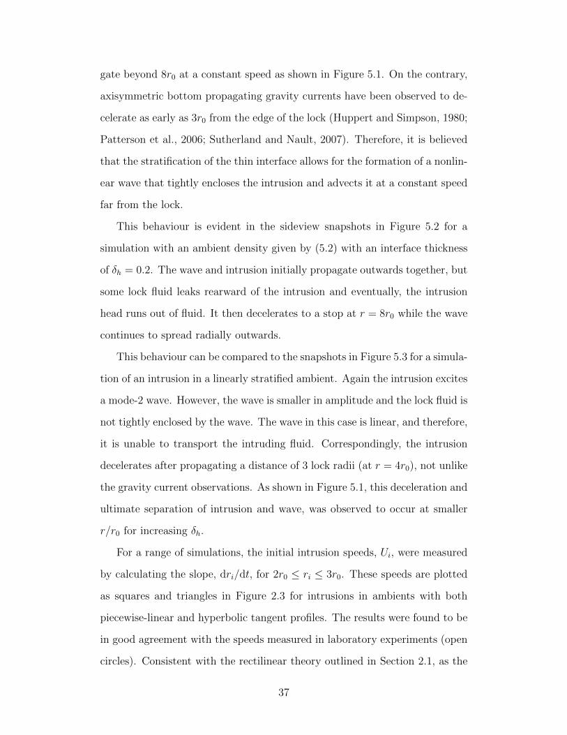
gate beyond 8r0 at a constant speed as shown in Figure 5.1. On the contrary,
axisymmetric bottom propagating gravity currents have been observed to de-
celerate as early as 3r0 from the edge of the lock (Huppert and Simpson, 1980;
Patterson et al., 2006; Sutherland and Nault, 2007). Therefore, it is believed
that the stratification of the thin interface allows for the formation of a nonlin-
ear wave that tightly encloses the intrusion and advects it at a constant speed
far from the lock.
This behaviour is evident in the sideview snapshots in Figure 5.2 for a
simulation with an ambient density given by (5.2) with an interface thickness
of δh = 0.2. The wave and intrusion initially propagate outwards together, but
some lock fluid leaks rearward of the intrusion and eventually, the intrusion
head runs out of fluid. It then decelerates to a stop at r = 8r0 while the wave
continues to spread radially outwards.
This behaviour can be compared to the snapshots in Figure 5.3 for a simula-
tion of an intrusion in a linearly stratified ambient. Again the intrusion excites
a mode-2 wave. However, the wave is smaller in amplitude and the lock fluid is
not tightly enclosed by the wave. The wave in this case is linear, and therefore,
it is unable to transport the intruding fluid. Correspondingly, the intrusion
decelerates after propagating a distance of 3 lock radii (at r = 4r0), not unlike
the gravity current observations. As shown in Figure 5.1, this deceleration and
ultimate separation of intrusion and wave, was observed to occur at smaller
r/r0 for increasing δh.
For a range of simulations, the initial intrusion speeds, Ui, were measured
by calculating the slope, dri/dt, for 2r0 ≤ ri ≤ 3r0. These speeds are plotted
as squares and triangles in Figure 2.3 for intrusions in ambients with both
piecewise-linear and hyperbolic tangent profiles. The results were found to be
in good agreement with the speeds measured in laboratory experiments (open
circles). Consistent with the rectilinear theory outlined in Section 2.1, as the
37

0 2 4 6 8 10t/t0
0
2
4
6
8
10
rir0
δh = 0.02δh = 0.20δh = 0.40δh = 0.60δh = 0.80δh = 1.00
Figure 5.1: The location of the intrusion front versus time for simulations withρL = 1.0530 g/cm3 and ρ(z) given by (2.1). At a thick interface (δh ≥ 0.60), theintrusion begins to decelerate around 3r0, whereas at a thin interface (δh ≤ 0.2)the intrusion maintains a constant speed beyond 8r0.
thickness of the interface increases, the intrusion speed decreases. However,
for all δh, axisymmetric intrusions were found to travel more slowly than the
predicted speed of intrusions in a rectilinear geometry, given by (2.4). This
implies that the curvature of the geometry has an effect on the initial intrusion
speed.
Figure 2.3 also shows that compared to the long-wave speed, symmetric in-
trusions travel more quickly if δh > 0.4 and hence the intrusion is supercritical.
This observation provides further evidence that at a sufficiently thin interface
the wave is nonlinear upon generation. Because nonlinear waves can transport
mass, intrusions in ambients with δh > 0.4 can be carried beyond 3 lock radii
at a constant speed, consistent with the results presented in Figure 5.1. On
the other hand, intrusions at thicker interfaces (δh > 0.4) are subcritical and
hence they excite linear waves, which are unable to transport mass.
Because the motivation of this work was to understand axisymmetric in-
38

Figure 5.2: Snapshots of the normalized vertical velocity field, w/wmax, ob-tained from a numerical simulation of an axisymmetric intrusion in an ambientfluid with a background density, ρt, given by Eq. (5.2) with a non-dimensionalinterface thickness of δh = 0.2. The thick black lines outline the intrusionprofile at each time and illustrate that the intrusion head is being carried out-ward by a wave. In each plot, the vertical velocity field is normalized by themaximum amplitude of the wave at t/t0 = 0.5, where t0 = r0/U0. The colour-bar limits are scaled by
√t/t0 − 0.5, making it evident that the amplitude of
the wave decays from its maximum value as t−1/2. The wave is observed topropagate at a constant speed (ie. r ∼ t); therefore, the amplitude of the waveis decreasing as r−1/2 as is predicted by linear theory.
39

Figure 5.3: Snapshots of the normalized vertical velocity field obtained froma numerical simulation of an axisymmetric intrusion in an ambient fluid witha linearly stratified background density. The colorbars are the same as thosein Figure 5.2 to illustrate that the magnitude of the wave is smaller in thisambient fluid. Futhermore, the generated waves move much slower and theintrusion fluid is not trapped, as in Figure 5.2.
40
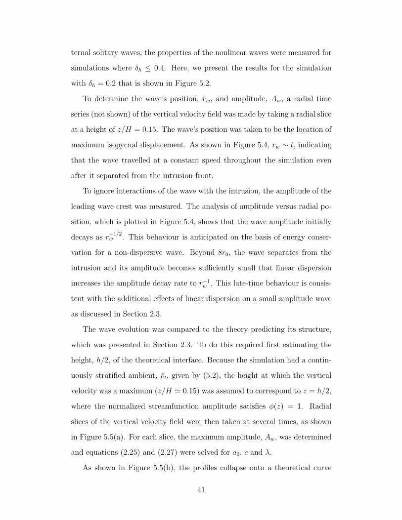
ternal solitary waves, the properties of the nonlinear waves were measured for
simulations where δh ≤ 0.4. Here, we present the results for the simulation
with δh = 0.2 that is shown in Figure 5.2.
To determine the wave’s position, rw, and amplitude, Aw, a radial time
series (not shown) of the vertical velocity field was made by taking a radial slice
at a height of z/H = 0.15. The wave’s position was taken to be the location of
maximum isopycnal displacement. As shown in Figure 5.4, rw ∼ t, indicating
that the wave travelled at a constant speed throughout the simulation even
after it separated from the intrusion front.
To ignore interactions of the wave with the intrusion, the amplitude of the
leading wave crest was measured. The analysis of amplitude versus radial po-
sition, which is plotted in Figure 5.4, shows that the wave amplitude initially
decays as r−1/2w . This behaviour is anticipated on the basis of energy conser-
vation for a non-dispersive wave. Beyond 8r0, the wave separates from the
intrusion and its amplitude becomes sufficiently small that linear dispersion
increases the amplitude decay rate to r−1w . This late-time behaviour is consis-
tent with the additional effects of linear dispersion on a small amplitude wave
as discussed in Section 2.3.
The wave evolution was compared to the theory predicting its structure,
which was presented in Section 2.3. To do this required first estimating the
height, h/2, of the theoretical interface. Because the simulation had a contin-
uously stratified ambient, ρt, given by (5.2), the height at which the vertical
velocity was a maximum (z/H ' 0.15) was assumed to correspond to z = h/2,
where the normalized streamfunction amplitude satisfies φ(z) = 1. Radial
slices of the vertical velocity field were then taken at several times, as shown
in Figure 5.5(a). For each slice, the maximum amplitude, Aw, was determined
and equations (2.25) and (2.27) were solved for a0, c and λ.
As shown in Figure 5.5(b), the profiles collapse onto a theoretical curve
41

1 10rwr0
0.1
1
1.5
Aw
Aw0
slope: -1/2
slope: -1
1
10
20
t−t ∗t0
slope: 1
Figure 5.4: The wave amplitude and position for the simulation shown inFigure 5.2 with δh = 0.2. The solid line shows the amplitude of verticalvelocity, Aw, versus radial position, rw, for the wave at a height of z/H = 0.15.A reference amplitude, Aw0 , is defined such that Aw = Aw0(rw/r0)−0.48 for2r0 ≤ rw ≤ 3r0. The circles correspond to t/t0 = 2.5, 5.0, 7.5 and 10.0, forwhich wave profiles are illustrated in Fig. 5.5. The radial position of the waveversus time is indicated by the dashed line. A reference time, t∗, is definedsuch that rw = drw
dt(t − t∗) for 4r0 ≤ rw ≤ 10r0. The curves are compared
with lines of constant slope as indicated.
when the amplitude is scaled by r−1/2w and the radial extent is shifted by
2r0 + c∆t and scaled by λ. It should be noted that the reference location
of 2r0 was chosen to ignore the initial generation of the wave caused by the
intrusion. For the intermediate times, t/t0 = 5.0 and 7.5, the simulation
results are in excellent agreement with the theory. However, at t/t0 = 10.0,
the wave amplitude became small and linear dispersion slightly increased the
broadening of the wave. The slight discrepancy at t/t0 = 2.5 can be explained
by the strong interaction between the wave and intrusion at early times.
These simulations of vertically symmetric intrusions are in good agreement
with the experimental results presented in Chapter 3 and the heuristic theory
for axisymmetric solitary waves presented in Chapter 2. The results are next
extended to oceanographic scales in an attempt to capture the essential dy-
42
2 4 6 8 10rr0
1
0
1
w
Aw0
(a)
t/t0 = 2.5
t/t0 = 5.0
t/t0 = 7.5
t/t0 = 10.0
0 1 2 3 4 5r−2r0−c∆t
λ
0.0
0.5
1.0
w Aw
0
( r 0 r w
)p
(b)
t/t0 = 2.5
t/t0 = 5.0
t/t0 = 7.5
t/t0 = 10.0
Theory
Figure 5.5: (a) Horizontal profiles of the vertical velocity field at a heightz/H = 0.15 for δh = 0.2. (b) Corresponding normalized and shifted profiles,where ∆t is the time elapsed since rw = 2r0, p = −1
2and Aw0 is a reference
amplitude defined in Fig. 5.4.
namics governing the wave generation process at the mouth of the Columbia
River.
43
Chapter 6
River Plumes
The motivation for this work is based in part on the observations of internal
solitary waves by satellite images (Jackson, 2004). Synthetic aperture radar
(SAR) images, which detect surface roughness, illustrate that internal soli-
tary waves in many locations of the world’s oceans have curved wavefronts.
This lateral spreading of the wavefronts occurs when they are generated by a
localized source and the motion is not restricted by a rectilinear domain.
As shown by experiments in Chapter 3 and by simulations in Chapter 5,
internal solitary waves can be launched by the flow of vertically symmetric
intrusions into a two-layer fluid with finite interface thickness. This is a sym-
metric expansion of a gravity current flowing along the surface of a fluid that
consists of a thin stratified layer overlying a deep layer of uniform-density fluid.
In nature, such gravity currents can manifest themselves in the form of river
plumes flowing into the coastal ocean. For example, in July 2004, measure-
ments of density and velocity fields were taken near the mouth of the Columbia
River revealing both the advance of the intruding river into the ocean and the
generation of waves at the pycnocline (Nash and Moum, 2005). Details of the
specific observations are described in Section 6.1.
Using the numerical code described in Chapter 4, simulations were per-
formed in an attempt to capture the essential dynamics of the Columbia River
44

plume. To do so, it was necessary to make many crude simplifications to the
oceanographic conditions. Regardless of this fact, the dynamics of the motion
were captured qualitatively and, for some measurements, quantitatively. Com-
parisons between the observations and the simulation results are presented in
Section 6.4.
6.1 Columbia River Plume
The Columbia River is the fourth largest river in the United States, flowing
into the Pacific Ocean at the border of Washington and Oregon. The depth
near the river mouth is approximately 20 m, increasing to 100 m within 15 km
of the coastline (Pan et al., 2007). The average flow rate from the Columbia
River is 7300 m3/s. However, during the spring months the flow rate may be
upwards of 15, 000 m3/s with ebb currents reaching 3.5 m/s (Jay et al., 2010).
SAR images and in situ measurements indicate that internal waves, manifest
as sinusoidal undulations of the pycnocline, are frequently launched ahead of
the plume (Nash and Moum, 2005; Pan et al., 2007; Stashchuk and Vlasenko,
2009), though details of the generation mechanism remain unclear.
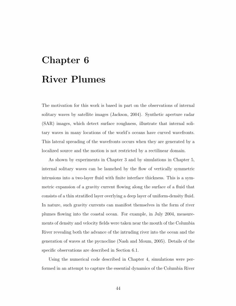
Here we focus on the in situ measurements that were made on July 23rd,
2004, which are presented in Nash and Moum (2005). Figure 6.1 shows three
snapshots of the sea surface temperature, where the plume front is approxi-
mated by the black contour. In total, nine transects across the plume front
were made, as indicated by the diamonds. Initially, at 17:21UTC, the plume
of warm summertime water flowed towards the northwest. At later times
(20:22UTC and 21:52UTC) the plume propagated eastward. These directions
are indicated in Figure 6.1 by the white velocity vectors.
At each transect of the plume front, a Chameleon turbulence profiler was
used to measure the density profiles and an Acoustic Doppler Current Profiler
was used to get the velocity profiles. Figure 6.2 shows these measurements at
45
Figure 6.1: Images of the sea surface temperature at the mouth of theColumbia River showing the progression of the plume on July 23rd, 2004 at (a)11:50, (b) 19:22, and (c) 21:31. The diamonds represent positions where theplume front was crossed and the red line represents the ship track. Measuredfluid velocities are indicated by the vectors and the 17◦C isotherm, which ap-proximates the plume front, is indicated by the black contour. The domainsize of each image is approximately 28 km in the N-S direction and 26 km inthe E-W direction. Reprinted by permission from Macmillan Publishers Ltd:Nature Publishing Group, from Figure 2 of Nash, J. D. and J. N. Moum.Nature. 437, 400 – 403 (2005).
four crossings. At 19:01UTC (Figure 6.2(a)) the plume flowed at a speed of
Uf ≈ 0.6 m/s against an ambient wind-driven current of Ua ≈ −0.1 m/s. From
the density measurements, it is evident that the plume of fresh water forced the
near surface waters to be displaced approximately 20 m downwards. One-and-
a-half hours later the plume’s speed decreased to 0.4 m/s and the internal wave
began to separate from the front (Figure 6.2(b)). The amplitude of the wave
at this time was ∼ 25 m. Approximately an hour later a second depression
of smaller amplitude separated from the plume front and trailed the leading
wave by ∼ 400 m (Figure 6.2(c)). In the final frame (Figure 6.2(d)) a total
of six waves are visible. At the ninth and final transect (not shown), a total
of seven waves were measured. All the waves propagated at a nearly constant
speed of cw ≈ 0.45 m/s. Nash and Moum (2005) also observed that the waves
46

were rank-ordered in that the largest amplitude wave was at the front of the
wave packet and each successive wave had a smaller amplitude. The distance
separating contiguous pairs of waves was also rank-ordered.
Using their measurements of the plume’s front speed, Nash and Moum
(2005) calculated two Froude numbers. The first, F = Uf/cw, was the ratio
of the front speed to the measured wave speed. The second, Fa = Uf/ca, was
the ratio of the front speed to the theoretical speed of a mode-1 linear wave
in the ambient, ca ≈ 0.4 m/s. The value of ca was determined by solving the
Taylor-Goldstein equation for the measured background density and velocity
fields. The definition of Fa is equivalent to the Froude number, Fr, introduced
in Section 2.2, though Fa is based on a measured, not theoretical, intrusion
speed. Hence, when Fa > 1 the current was supercritical and the generation of
solitary waves was expected. Initially, both F and Fa were greater than unity,
but as the plume decelerated, the Froude numbers decreased. When F ≈ 1, at
which time Fa ≈ 1.1, the leading wave separated from the plume front. Nash
and Moum (2005) diagnosed wave fission to occur when F = 1. Because the
definition of F is based on the measured, not the theoretical, wave speed it
is not useful in predicting the exact fission location for an arbitrary ambient.
However, it is useful to note that Fa is only slightly greater than unity at the
time of fission.
The measurements made by Nash and Moum (2005) are summarized in
Table 6.1.
6.2 Approximations and the Simulation Setup
The intent here is not to perform a realistic simulation of the Columbia River
plume. Rather, it is to use a simple model that attempts to capture the essen-
tial dynamics of the wave generation process. Thus many approximations are
made. The wind-driven surface currents and topography in the coastal region
47

Figure 6.2: Measurements of density, acoustic backscatter and velocity madeabout 10 km from the mouth of the Columbia River on July 23rd, 2004. (a)Internal waves grow at the front of the plume. (b) Initial separation of theinternal wave from the plume front. (c) Separation of a second wave from theplume front. (d) Large amplitude internal waves propagate freely ahead ofthe plume. The inset shows the density profile that was measured for Pass 4(panel a). Reprinted by permission from Macmillan Publishers Ltd: NaturePublishing Group, from Figure 3 of Nash, J. D. and J. N. Moum. Nature. 437,400 – 403 (2005).
48

are omitted: there is no initial ambient motion and the depth is constant.
Furthermore, the numerical code requires the background density profile to
be constant in r and t, whereas in reality the stratification changes both with
location and time.
The forcing conditions also differ significantly. As explained by Nash and
Moum (2005), the river plume is released when ebb currents begin to flow,
immediately following high tide. Rather than simulate the exact influence of
the tides by including a time-variable momentum flux at the source, a partial-
depth lock-release initial condition was used to generate the surface gravity
current.
Due to the code’s boundary conditions that require the flow to be irrota-
tional at the bottom and top of the domain, it is difficult to maintain numerical
stability in the simulation of a surface gravity current; the flow is not neces-
sarily irrotational at the front itself. Instead, a vertically symmetric intrusion
was simulated and the analysis was carried out in the lower half of the domain
where −H2≤ z ≤ 0. This symmetry was exploited, for example, in Section 2.1
in the derivation of the rectilinear intrusion speed.
The study of the Columbia River plume by Pan et al. (2007) indicated
that the coastal ocean depth in the region where the waves were observed was
about 100 m. Therefore the domain half-height was chosen to be H2
= 100 m.
Two different background density profiles, which are shown in Figure 6.3
for z < 0, were used in these river plume simulations. To ensure that the
intruding fluid propagated along z = 0, both of the density profiles were odd
functions with respect to z about the density at z = 0 (not shown).
The initial profile, denoted by ρST(z), is an analytic idealization of the
actual Columbia River data. The values of the densities were estimated based
on the profile presented in the inset of Figure 6.2, where the densities at
z = −5 m and z = −40 m were approximately 1023 kg/m3 and 1028 kg/m3,
49

1016 1020 1024 1028ρ(z) [kg/m3 ]
90
60
30
0
z [m
]
ρST(z)
ρCR(z)
Columbia River Data
Figure 6.3: The background density profiles, ρST(z) and ρCR(z), used for theriver plume simulations in comparison with data measured on July 23, 2004(Nash and Moum, 2005)(or other reference). Here, only the lower half of thedomain, z < 0, is shown. The actual profiles were odd functions with respectto z.
respectively. A hyperbolic tangent profile was used for the majority of the
simulation profile. However, the density at the three points below z = 0
varied linearly in z such that ρST(0) = ρi. This was done to maintain numerical
stability by minimizing the magnitude of the density jump at the interface.
As is shown in Figure 6.3, ρST(z) moderately overestimated the measured
densities, but it still captured a thin stratified region overlying a deeper region
of constant density.
In the actual data presented in Nash and Moum (2005) the density in
the upper 10 m of the ocean was nearly uniform. To examine its influence,
additional simulations with a density profile denoted by ρCR(z) were performed
in which the measured data were interpolated onto the computational grid, as
shown in Figure 6.3. Below a depth of 60 m, it was assumed that the density
was constant because there was no data in this region. Furthermore, the
50

densities at the two points near the surface were modified to minimize the
magnitude of the density jump at z = 0.
The initial density field for the simulations was given by
ρinit(r, z) =
{ρi 0 < r < r0, −Hm
2< z < Hm
2
ρ(z) elsewhere,(6.1)
where r0 is the lock radius and Hm is the total height of the mixed region in
the lock. In an effort to simulate the scale of the Columbia River plume, the
lock diameter, 2r0, was chosen to be 5 km, which is the approximate width of
the river’s mouth. To control the volume of the collapsing fluid, the value of
Hm
2was varied from 20 m to 70 m in increments of 10 m. The density of the
intruding fluid, ρi, was set to 1015 kg/m3, which was the approximate density
of the Columbia River plume on July 23rd, 2004 (Nash and Moum, 2005).
As was described in Section 4.3, a spatially varying viscosity was used to
damp out the small scale noise arising from the collapse of the mixed fluid.
In order to obtain a nearly uniform Reynolds number, a different viscosity
was chosen for each Hm. The value of νout where r > 3.2 km increased from
0.02 m2/s for Hm
2= 20 m to 0.09 m2/s for Hm
2= 70 m. For all simulations, the
viscosity where r < 2.7 km was set to νin = 5νout and between r = 2.7 km and
r = 3.2 km the viscosity varied linearly as given by (4.14). Upon completing
the simulations, the Reynolds numbers, Re =UfHm
νout, were determined to vary
between 2070 and 2760. The diffusivity, κ, was chosen so that the Schmidt
number, Sc = νout/κ, was equal to 10 for all simulations. Both the viscosity
and the diffusivity were much greater than the physical values in order to
maintain numerical stability. The passive tracer diffusivity, κPT, was set equal
to κ for all simulations.
The radial extent of the domain was chosen to be R = 10 km because
beyond this distance the wave amplitude was sufficiently small that the motion
was dominated by viscosity. The grid contained 5000 points in the radial
51

direction and 128 points in the vertical direction.
The majority of runs simulated the evolution of the river plume and waves
for at least 4000 s with a timestep of 0.5 s; however, a timestep of 0.25 s was
required to maintain numerical stability for Hm
2= 70 m. Snapshots of the
density, velocity and vorticity fields were output every 10 s. Due to the large
domain size, each simulation took at least 8 days to complete.
6.3 Analysis and Results
Qualitatively similar to observations, the propagation of the simulated river
plume launched a train of freely propagating internal waves. This is shown
for Hm
2= 50 m in Figure 6.4 for a simulation with analytically prescribed
ambient density (ρ = ρST) and in Figure 6.5 for a simulation with interpolated
Columbia River ambient density (ρ = ρCR). In these figures, the black line
denotes the 1023 kg/m3 isopycnal.
More waves were launched in the simulation using ρ = ρST than in the
simulation using ρ = ρCR. This comparison is consistent for all values of Hm
2,
as shown in Table 6.1. The reason less waves appear when ρ = ρCR can be
attributed to the structure of the upper mixed region in that ambient density
profile. The large density jump at z ≈ −10 m can be approximated by a
strongly stratified region between two layers of uniform density. When long
waves propagate in such an ambient fluid, shear is introduced across the strat-
ified interface. This shear causes the flow to go unstable which, in turn, causes
some of the wave energy to be converted into mixing. The necessary condi-
tion for the instability of a parallel stratified shear flow is that the Richardson
number satisfies Ri > 1/4. Generalizing the definition of Ri, at all points in
the domain we estimate
Ri(r, z) ≈ N2T
ζ2, (6.2)
52

40
20
0
z [m
]
(a) t=500 s
1018 1028
40
20
0
z [m
]
(b) t=1500 s
40
20
0
z [m
]
(c) t=2500 s
0 2000 4000 6000 8000r [m]
40
20
0
z [m
]
(d) t=3500 s
Figure 6.4: Snapshots of the total density field in units of kg/m3 from asimulation with ρ = ρST and Hm
2= 50 m. The black line is the 1023 kg/m3
isopycnal. Only a subsection of the total domain is shown as R = 10 000 mand H
2= 100 m. It should be noted that the simulated plume is propagating
from left to right in this figure, whereas the observed plume in Figure 6.2 ispropagating from right to left.
53
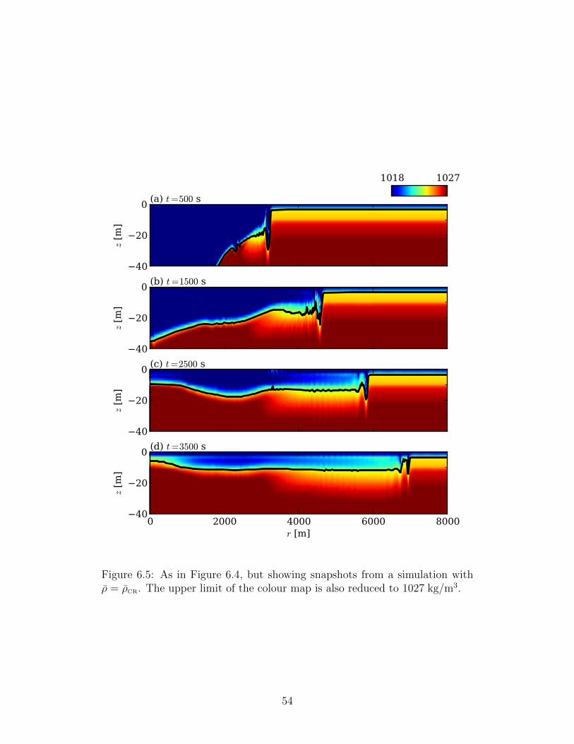
40
20
0
z [m
]
(a) t=500 s
1018 1027
40
20
0
z [m
]
(b) t=1500 s
40
20
0
z [m
]
(c) t=2500 s
0 2000 4000 6000 8000r [m]
40
20
0
z [m
]
(d) t=3500 s
Figure 6.5: As in Figure 6.4, but showing snapshots from a simulation withρ = ρCR. The upper limit of the colour map is also reduced to 1027 kg/m3.
54
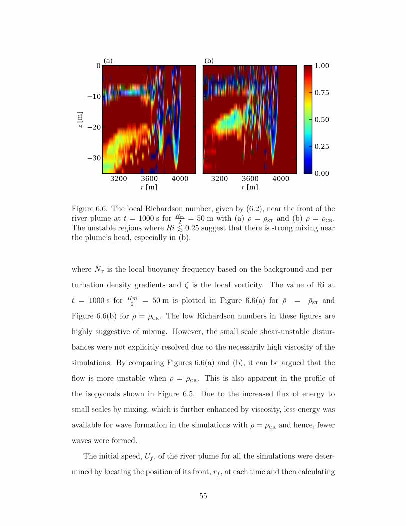
3200 3600 4000r [m]
30
20
10
0
z [m
]
(a)
3200 3600 4000r [m]
(b)
0.00
0.25
0.50
0.75
1.00
Figure 6.6: The local Richardson number, given by (6.2), near the front of theriver plume at t = 1000 s for Hm
2= 50 m with (a) ρ = ρST and (b) ρ = ρCR.
The unstable regions where Ri > 0.25 suggest that there is strong mixing nearthe plume’s head, especially in (b).
where NT is the local buoyancy frequency based on the background and per-
turbation density gradients and ζ is the local vorticity. The value of Ri at
t = 1000 s for Hm2
= 50 m is plotted in Figure 6.6(a) for ρ = ρST and
Figure 6.6(b) for ρ = ρCR. The low Richardson numbers in these figures are
highly suggestive of mixing. However, the small scale shear-unstable distur-
bances were not explicitly resolved due to the necessarily high viscosity of the
simulations. By comparing Figures 6.6(a) and (b), it can be argued that the
flow is more unstable when ρ = ρCR. This is also apparent in the profile of
the isopycnals shown in Figure 6.5. Due to the increased flux of energy to
small scales by mixing, which is further enhanced by viscosity, less energy was
available for wave formation in the simulations with ρ = ρCR and hence, fewer
waves were formed.
The initial speed, Uf , of the river plume for all the simulations were deter-
mined by locating the position of its front, rf , at each time and then calculating
55

20 30 40 50 60 70Hm
2
1.0
1.2
1.4
1.6
Uf
[m/s
]
[m]
ρST(z)ρCR(z)
Figure 6.7: Initial speeds of the leading wave, and hence the river plume, asdetermined by calculating drf/dt from t = 150 s to t = 450 s.
the slope, drf/dt, between t = 150 s and t = 450 s. These speeds are plotted
versus Hm
2in Figure 6.7. This shows that Uf increases with Hm
2, as expected,
because the initial available potential energy that is partially converted to ki-
netic energy of the plume is proportional to H2m. Figure 6.7 also shows that,
for given Hm
2, the river plume in the ambient with ρ = ρST travelled on average
2% faster than those in ambients with ρ = ρCR. The relatively small difference
in speeds implies that the advance of the plume is relatively insensitive to the
structure of the density profiles that were used.
The analysis of these simulations involved calculating the speed and ampli-
tude of each wave for various times. To do so, the location of the 1023 kg/m3
isopycnal was found every 10 s. From the resulting profile, the position of
each wave was determined from the radial location of each local minima. The
wave position rw was then plotted versus time, as shown in Figure 6.8(a) for
Hm
2= 50 m and ρ = ρST.
56
For each wave, the average speed cw was calculated every 300 s by calcu-
lating the slope, drw/dt, over a 300 s interval. As shown in Figure 6.8(b), the
wave speeds decreased with time and eventually all the waves attained a simi-
lar speed. The initial speeds of the leading waves were equal to the front speed,
Uf , because the plume and the wave initially propagated together. Eventu-
ally, the wave separated from the plume front. Admittedly, though, it was
difficult to determine the exact location of wave fission because the density of
the intruding plume was the same as that just ahead of it. Furthermore, the
high diffusivity of the passive tracer field made it an unreliable indictor for the
location of the plume at late times.
Figure 6.4 shows that waves develop successively, one after the other, even-
tually forming a wave train of crests and troughs. This is quantified in Fig-
ure 6.8. The leading wave is launched almost immediately (at t ≈ 60 s) whereas
the second wave forms around t ≈ 550 s. At this time, the second wave is ap-
proximately 130 m behind the first and, because the leading wave is initially
travelling faster than the second wave (see Figure 6.8(b)), the distance sep-
arating the waves grows. The maximum separation distance ∆r12 ≈ 250 m
is eventually attained when the waves reach a similar speed. This trend was
observed for all the simulations with ρ = ρST and the ∆r12 values are given
in Table 6.1. For these simulations, the separation distance does not depend
significantly on Hm
2. All values lie between 210 m and 280 m, suggesting that
∆r12 is set by the background density profile, not the speeds of the waves.
Additional measurements (not shown) indicate that the distance separating
successive waves decreases (ie. ∆r12 > ∆r23 > ∆r34).
The approximate values of ∆r12 are given in Table 6.1 for the simulations
with ρ = ρCR. Due to the enhanced mixing that occurs in these simulations, it
was sometimes difficult to locate the exact position of the waves. In some cases
a steady separation distance was not attained in the time of the simulation.
57

2000
4000
6000
8000
r w [
m]
(a)
Wave 1Wave 2Wave 3Wave 4
0 1000 2000 3000 4000time [s]
1.0
1.2
1.4
1.6
c w [
m/s
]
(b)
Figure 6.8: Six waves were formed in the simulation with Hm
2= 50 m and
ρ = ρST (see Figure 6.4). The positions, rw, of the first four waves weremeasured from r = 0 are plotted versus time in (a) and the average speeds,cw, of the first four waves which were calculated every 750 s are shown in (b).In comparison, the mode-1 wave speed, ca, for ρ = ρST is 0.67 m/s.
58

3000 4000 5000 6000 7000 8000rw [m]
0
5
10
15
20
25
30
Aρc [
m]
Wave 1Wave 2Wave 3Wave 4
Figure 6.9: The magnitude of the isopycnal displacement for ρc = 1023 kg/m3
versus position for the simulation with ρ = ρST and Hm
2= 50 m. Although
six waves were observed (see Figure 6.4), only the amplitude for the first fourwaves is plotted.
This is indicated in Table 6.1 by the asterisks.
In the snapshots in Figures 6.4 and 6.5 it is evident that the amplitudes
of the waves decrease as they propagate outwards. The displacement of the
isopycnal troughs were measured relative to the upstream position, and are
plotted versus position in Figure 6.9 for the simulation shown in Figure 6.4.
After an initial increase in amplitude during the generation of the wave, the
amplitude decreases approximately linearly with r. It is expected that the am-
plitude should obey an inverse power law for sufficiently large r. In particular,
a single inviscid wave should decay in amplitude as r−1/2. However, the simu-
lations were not run long enough to observe this trend. Due to the damping of
the motion by the artificially high viscosity we expect the amplitude to decay
more rapidly than A ∼ r−1/2.
It is also evident in both Figures 6.4 and 6.9, that at any given time the
waves are rank-ordered. That is, the amplitude of each successive wave is
59

smaller than the one ahead it (ie. A1 > A2 > A3). The maximum amplitudes
of the leading waves, Amax = max(A1), for all the simulations are summa-
rized in Table 6.1. As expected, the maximum wave amplitude increases with
increasing Hm
2. Furthermore, Amax does not vary significantly between simu-
lations with the two different background density profiles.
6.4 Discussion
Despite the omission of tides, surface currents and bottom topography, the sim-
ulations were in good qualitative, and in somewhat good quantitative agree-
ment with the observations presented in Nash and Moum (2005). In this
section, the observations discussed in Section 6.1 will be compared to the sim-
ulations with Hm
2= 50 m because the initial amplitudes of the observed and
simulated wave were approximately equal (see Table 6.1).
Figures 6.4 and 6.5 clearly show that the surface-propagating gravity cur-
rent launches a train of freely-propagating internal waves which are formed in
succession, qualitatively consistent with the observations of Nash and Moum
(2005).
Nash and Moum (2005) observed a total of seven freely propagating waves.
In comparison, the number of waves in the simulations varied from 2 to 6 with
less (2–3) waves being generated in simulations with ρ = ρCR, the ambient
density interpolated from the observed data. There are several possible rea-
sons for this discrepancy. As explained in Section 6.3, there appeared to be
enhanced mixing in simulations with ρ = ρCR, which reduced the amount of
energy available for wave formation. Furthermore, the measured density pro-
file shown in Figure 6.3 was observed at a specific instant in time at a specific
location, whereas the stratification likely varied throughout the observation
region, having a significant effect on wave formation. The wind-driven surface
currents that were observed by Nash and Moum (2005) also helped the wave
60

Speed Amplitude Wave Separation No. of WavesHm
2Uf Amax ∆r12
(m) (m/s) (m) (m)
Columbia River Observations
0.7 20 - 25 400 7
ρST(z)
20 1.1 11 220 630 1.3 17 210 640 1.4 22 240 650 1.5 27 250 660 1.6 32 260 570 1.6 36 280 5
ρCR(z)
20 1.0 11 150 330 1.3 16 150* 340 1.4 23 170 350 1.5 29 220 260 1.6 34 280 270 1.6 38 250* 3
Table 6.1: Data from the river plume simulations in comparison with the ob-servations made by Nash and Moum (2005). The initial speed of the riverplume is denoted by Uf . For the observations, Uf was measured at 17:21UTC
and for the simulations Uf was computed at t = 300 s. The maximum dis-placement of the 1023 kg/m3 isopycnal of the leading wave is denoted by Amaxand the maximum separation distance attained between the first and secondwaves is denoted by ∆r12. The * indicates that the separation distance wasincreasing or decreasing rather than remaining constant.
61

formation by increasing the convergence of horizontal velocities at the plume
front. Of all these reasons, it is most likely the artificially high viscosities
that caused fewer waves to form in the simulations. At late times, when the
wave amplitudes and speeds were small, the motion was significantly damped
preventing the formation of additional waves. This conclusion was made on
the basis of simulations (not shown) with still higher viscosities, in which only
1–2 waves formed.
The simulated location of the initial wave fission is significantly different
from the observed location with respect to the river mouth. As shown in
Figure 6.2(b), the leading wave separated from the plume front at roughly
19:25UTC, at which time the plume was roughly 12−15 km from the mouth of
the Columbia River (determined from Figure 6.1). In simulations, the initial
wave fission occurred within 500 m of the lock (for Hm
2= 50 m). As mentioned
in Section 6.3, it was difficult to determine the exact location of wave fission
from the simulations because the density of the intruding fluid was the same as
that just ahead of it. Because the second wave formed around r = 3000 m (see
Figure 6.8), it was assumed that the wave fission occurred prior to the intrusion
reaching this location. The reason for the discrepancy between the simulations
and the observations is likely due to the initial conditions: the simulations
used an instantaneous constant-volume release to generate a gravity current,
whereas the Columbia River plume is better represented by gradual increase
in volume flux at the source while the tide ebbs. Based on a mean flow rate
of 1 m/s and a semidiurnal tide (Jay et al., 2010), the maximum volume flux
occurs approximately 3.1 hours following high tide at a distance of 11 km from
the mouth of the Columbia River. It is at this location that a lock-release best
describes the plume. Therefore, it can be argued that the simulation results
are consistent with the observation of waves being generated 12− 15 km from
the mouth of the river.
62
Another comparison can be made in regards to the plume speeds and
Froude numbers. Although the initial front speed measurements differ by
up to a factor of 2 (see Table 6.1), the river plume decelerates as it propagates
outwards in both the simulations and the observations. On the other hand,
the observed wave speeds were approximately constant at 0.45 m/s, while the
simulated initial wave speed for Hm
2= 50 m was 1.5 m/s and then decreased
throughout the simulation by up to 50%, as shown in Figure 6.8(b). The de-
creasing values of cw in time make it difficult to determine a Froude number
with respect to the wave speed, F = Uf/cw, as was done by Nash and Moum
(2005).
It is possible, however, to calculate a linear long wave speed for the ambient,
ca, by solving the Taylor-Goldstein equation. To do so, a Matlab program
(Smyth et al., 2010) was used to calculate the mode-1 wave speed. Explicitly,
ca ' 0.67 and 0.65 m/s for ρ = ρST and ρCR, respectively. In comparison, Nash
and Moum (2005) calculated ca ' 0.4 m/s, but this computation included
the measured background horizontal velocity field. For all the simulations,
the initial plume speeds were significantly larger than ca (see Figure 6.7).
Hence, Fa > 1 and solitary waves were launched. Due to the high diffusivity
of the passive tracer field, it was difficult to measure the plume speeds, and
consequently Fa, at late times. However, the speeds of the waves (shown in
Figure 6.8) suggest that Fa > 1.5 for the entire duration of the simulation. In
comparison, Nash and Moum (2005) observed that the initial wave separated
from the front of the plume when Fa ≈ 1.1 and Fa decreased to less than unity
by the fifth measurement of the plume’s speed.
Nash and Moum (2005) measured a 20 − 25 m amplitude for the leading
wave, which compared well with the simulations in cases where Hm
2was equal
to 40 m or 50 m. In the simulations, the wave amplitude decreased rapidly
as shown in Figure 6.9. However, Nash and Moum (2005) reported that the
63

amplitude remained constant for nearly 5 km. Due to the axisymmetric ge-
ometry, the amplitude decay is expected. Therefore, their observed constant
amplitude must be attributed to other factors. A possible explanation is that
at the time of the measurements, the observed wave front (black line in Fig-
ure 6.1) is more or less planar; since the wave is not spreading radially, a
constant amplitude would be expected.
There is qualitatively good agreement between the observations and the
simulations in that the amplitude of each successive wave was smaller than the
one ahead of it. This is apparent in Figure 6.2(d) for the observed waves and in
Figure 6.9 for the simulated waves. The decreased amplitude can be attributed
to the reduced convergence at the front of each wave and the observation
of rank-ordered waves is consistent with other observations of solitary wave
packets (Jackson, 2004).
A final comparison between the observations and the simulations can be
made with respect to the spacing between contiguous waves. Figure 6.2(d)
shows that the maximum distance between the leading wave and the second
wave, ∆r12, is about 400 m. In comparison, the maximum distance measured
in the simulations varies between 150 m and 280 m. Although the magni-
tude of the separation is significantly different, both the simulations and the
observations show that the distance between successive waves decreases.
In general, despite the approximations of the numerical model, the simu-
lations were found to be in good qualitative agreement with the observations:
the propagation of a river plume into the coastal ocean launches a train of
freely-propagating internal waves that are rank-ordered with respect to their
amplitudes and separation distances. Because the intent of these simulations
was to capture the essential dynamics of the wave generation process, we can
also argue, for Hm
2= 40 m or 50 m, that the wave characteristics are is good
quantitative agreement with the observed wave speeds and amplitudes.
64

Chapter 7
Summary and Conclusions
We have studied the dynamics of axisymmetric internal solitary waves by
way of theory, experiments and numerical simulations. Although this work
was motivated by the observation of curved wave fronts advancing ahead of
river plumes in the coastal ocean, we began by investigating the launch of
these waves by vertically symmetric intrusions in a two-layer fluid with finite
interface thickness. We then adapted the idealized study to more realistic
oceanographic circumstances and compared the results with observations of
the Columbia River plume.
In the study of vertically symmetric intrusions, a theory was derived to
predict the speed of such an intrusion as a function of the interface thickness.
Unlike previous estimates (Ungarish, 2005; White and Helfrich, 2008), our
theoretical prediction was in agreement with the recent experiments by Bolster
et al. (2008).
Laboratory experiments and numerical simulations of vertically symmetric
intrusions were conducted in a cylindrical geometry. In agreement with the
theory, the intrusion speed was dependent upon the non-dimensional thickness
of the interface, decreasing from 0.8U0 to 0.5U0 as δh increased from 0 to 1.
These speeds were up to 20% slower than those of intrusions in a rectilinear
geometry.
65

From the observation that the experimental intrusions propagated well be-
yond 3 lock radii at a constant speed, it was hypothesized that a closed-core
solitary wave surrounded the intrusion and carried it outwards. In addition
to confirming the presence of this wave at interfaces satisfying 0 < δh . 0.4,
the simulations were used to obtain more information about the wave char-
acteristics. The wave carried the intrusion to approximately 7 lock radii as
its amplitude decreased as r−1/2, a power law consistent with energy conser-
vation. Beyond this distance, the intrusion ran out of fluid and decelerated
to a stop, whereas the wave continued to propagate at a constant speed. Due
to the additional effect of linear dispersion, the rate of wave amplitude decay
increased to r−1 beyond 7 lock radii.
Profiles of the wave just above the intrusion head were compared to a recti-
linear solitary wave KdV theory adapted to a cylindrical geometry in which the
wave amplitude decreased as r−1/2. The wave profiles collapsed onto a theoret-
ical curve suggesting that the amplitude decay was slow enough that it did not
significantly affect the propagation of the wave. From a single measurement
of wave amplitude and the assumption that the amplitude decays as r−1/2,
this heuristic KdV theory is able to predict the amplitude, speed and spread
of the wave during its nonlinear evolution phase after generation. The fact
that the solitary wave evolved in a manner closer to the heuristic prediction
than to the rigorous cylindrical solitary wave equation suggests that a different
mathematical approach should be taken in developing an appropriate weakly
nonlinear theory. Because the adapted KdV theory did not account for the
leaky closed-core behaviour of the wave, it is suggested that future investiga-
tion could adapt the Dubreil-Jacotin-Long equation to a cylindrical geometry;
this equation has been used to describe closed-core (Davis and Acrivos, 1967;
Tung et al., 1982) and leaky (Derzho and Grimshaw, 2007) solitary waves in
a rectilinear geometry.
66

The numerical code was also used to simulate a river plume emanating
from the mouth of the Columbia River. In essence, this involved prescribing
more realistic ambient density profiles and allowing the intrusion to emanate
from a partial-depth mixed region. In contrast to the simulations of vertically
symmetric intrusions, which launched a single wave, a freely propagating train
of internal solitary waves was launched by the simulated river plume.
The development of a freely propagating train of waves was consistent with
the observations made by Nash and Moum (2005) in July 2004 of a plume
emanating from the Columbia River. There was also qualitative agreement
between the simulations and the observations in that the waves formed one at
a time with each successive wave having a smaller amplitude. Furthermore,
the separation distance between contiguous waves decreased with each succes-
sive wave pair. Quantitatively, it can be argued that the magnitudes of the
speeds and amplitudes are of the same order. This was somewhat surpris-
ing considering the number of approximations that were made. In particular,
wind-driven surface currents and bottom topography were omitted in the sim-
ulations. Furthermore, a constant-volume lock-release was used to simulate
the river outflow and a constant stratification (in r and t) was used for the
ambient fluid. These limitations had the most effect in the Froude number
criterion for wave fission. Nash and Moum (2005) observed that the leading
wave separated from the plume when Fa ≈ 1.1 and eventually Fa was less than
unity. In contrast, Fa > 1.5 for the duration of the simulations.
Further investigation is necessary to generalize our results to make pre-
dictions about the realistic propagation of river plumes in the coastal ocean.
A better understanding of the dynamics of these plumes and the waves they
generate is important for predicting the transport of nutrients, sediments and
pollutants in the local region. Higher resolution simulations with lower viscos-
ity would be beneficial as the motion of the river plume at late times seemed
67

to be dominated by viscosity. More specifically, the fact that the amplitude
decayed more rapidly than r−1/2 suggests that energy was being dissipated due
to viscosity. It would also be useful to have in situ data for plumes emanating
from different rivers. This could provide additional insight into how parame-
ters such as stratification, wind-driven currents, or bottom topography affect
the formation and propagation of the waves. At this time, however, only the
Columbia River plume has been examined in detail for its ability to generate
internal solitary waves.
68

Bibliography
Benjamin, T. B. (1968). Gravity currents and related phenomena. J. Fluid
Mech. 31, 209–248.
Benney, D. J. (1966). Long nonlinear waves in fluid flows. J. Math. and
Phys. 45, 52–63.
Bolster, D., A. Hang, and P. F. Linden (2008). The front speed of intrusions
into a continuously stratified medium. J. Fluid Mech. 594, 369–377.
Britter, R. E. and J. E. Simpson (1981). A note on the structure of the head
of an intrusive gravity current. J. Fluid Mech. 112, 459–466.
Davis, R. E. and A. Acrivos (1967). Solitary internal waves in deep water. J.
Fluid Mech. 29, 593–607.
Derzho, O. G. and R. Grimshaw (2007). Asymmetric internal solitary waves
with a trapped core in deep fluids. Phys. Fluids 19, Art. No. 095102.
Didden, N. and T. Maxworthy (1982). The viscous spreading of plane and
axisymmetric gravity currents. J. Fluid Mech. 121, 27–42.
Dubreil-Jacotin, M. K. (1937). Sur les theoremes d’existence relatifs aux ondes
permanentes perodiques a deux dimensions dans les liquides heterogenes. J.
Math. Pures Appl. 16, 43.
Faust, K. M. and E. J. Plate (1984). Experimental investigation of intrusive
69
gravity currents entering stably stratified fluids. J. Hydraul. Res. 22 (5),
315–325.
Hallworth, M. A., H. E. Huppert, J. C. Phillips, and R. S. J. Sparks (1996).
Entrainment into two-dimensional and axisymmetric turbulent gravity cur-
rents. J. Fluid Mech. 308, 289–311.
Halpern, D. (1971). Observations of short period internal waves in Mas-
sachusetts Bay. J. Mar. Res. 29, 116–132.
Helfrich, K. R. and W. Melville (2006). Long nonlinear internal waves. Annu.
Rev. Fluid Mech. 38, 395–425.
Hoult, D. P. (1972). Oil spreading on the sea. Ann. Rev. Fluid Mech. 4,
341–368.
Huppert, H. E. (1982). The propagation of two-dimensional and axisymmetric
viscous gravity currents over a rigid horizontal surface. J. Fluid Mech. 121,
43–58.
Huppert, H. E. and J. E. Simpson (1980). The slumping of gravity currents.
J. Fluid Mech. 99, 785–799.
Huq, P. (1996). The role of aspect ratio on entrainment rates of instantaneous,
axisymmetric finite volume releases of dense fluid. J. Hazardous Mater. 49,
89–101.
Jackson, C. R. (2004). An atlas of internal solitary-like waves and their proper-
ties (2nd ed.). Technical report, Global Ocean Associates. Available online
at www.internalwaveatlas.com.
Jay, D. A., E. D. Zaron, and J. Pan (2010). Initial expansion of the Columbia
River tidal plume: Theory and remote sensing observations. J. Geophys.
Res. 115, Art. No. C00B15.
70

Long, R. R. (1953). Some aspects of the flow of stratified fluids. I. A theoretical
investigation. Tellus 5, 42–58.
Long, R. R. (1956). Solitary waves in one- and two-fluid systems. Tellus 8,
460–471.
Lowe, R. J., P. F. Linden, and J. W. Rottman (2002). A laboratory study of
the velocity structure in an intrusive gravity current. J. Fluid Mech. 456,
33–48.
Maxworthy, T. (1980). On the formation of nonlinear internal waves from the
gravitational collapse of mixed regions in two and three dimensions. J. Fluid
Mech. 96, 47–64.
McMillan, J. M. and B. R. Sutherland (2010). The lifecycle of axisymmetric
internal solitary waves. Nonlin. Proc. Geophys. 17, 443–453.
Mehta, A., B. R. Sutherland, and P. J. Kyba (2002). Interfacial gravity cur-
rents. II. Wave excitation. Phys. Fluids 14, 3558–3569.
Miles, J. W. (1978). An axisymmetric Boussinesq wave. J. Fluid Mech. 84,
181–191.
Nash, J. D. and J. N. Moum (2005). River plumes as a source of large-
amplitude internal waves in the coastal ocean. Nature 437, 400–403.
Pan, J., D. A. Jay, and P. M. Orton (2007). Analyses of internal solitary
waves generated at the columbia river plume front using SAR imagery. J.
Geophys. Res. 1112, Art. No. C07014.
Patterson, M. D., J. E. Simpson, S. B. Dalziel, and G. L. F. van Heijst (2006,
APR). Vortical motion in the head of an axisymmetric gravity current.
Phys. Fluids 18 (4), Art. No. 046601.
71

Perry, R. B. and G. R. Schimke (1965). Large amplitude internal waves ob-
served off the north-west coast of Sumatra. J. Geophys. Res. 70, 2319–2324.
Rooij, F., P. F. Linden, and S. B. Dalziel (1999). Saline and particle-driven
interfacial intrusions. J. Fluid Mech. 389, 303–334.
Rottman, J. W. and J. E. Simpson (1983). Gravity currents produced by
instantaneous releases of a heavy fluid in a rectangular channel. J. Fluid
Mech. 135, 95–110.
Simpson, J. E. (1997). Gravity Currents (2nd ed.). Cambridge, England:
Cambridge University Press.
Smyth, W. D., J. N. Moum, and J. D. Nash (2010). Narrowband oscillations
in the upper equatorial ocean. Part II: Properties of shear instabilities. J.
Phys. Oceanogr., Submitted June 29.
Stashchuk, N. and V. Vlasenko (2009). Generation of internal waves by a
supercritical stratified plume. J. Geophys. Res. 114, Art. No. C01004.
Sutherland, B. R. and J. T. Nault (2007). Intrusive gravity currents propa-
gating along thin and thick interfaces. J. Fluid Mech. 586, 109–118.
Tung, K. K., T. F. Chan, and T. Kubota (1982). Large amplitude internal
waves of permanent form. Stud. Appl. Math. 66, 1–44.
Ungarish, M. (2005). Intrusive gravity currents in a stratified ambient:
Shallow-water theory and numerical results. J. Fluid Mech. 535, 287–323.
Ungarish, M. (2006). On gravity currents in a linearly stratified ambient:
A generalization of Benjamin’s steady-state propagation results. J. Fluid
Mech. 548, 49–68.
72

Weidman, P. D. and M. G. Velarde (1992, Feb). Internal solitary waves. Stud.
Appl. Math. 86 (2), 167–184.
Weidman, P. D. and R. Zakhem (1988). Cylindrical solitary waves. J. Fluid
Mech. 191, 557–573.
White, B. L. and K. R. Helfrich (2008). Gravity currents and internal waves
in a stratified fluid. J. Fluid. Mech. 616, 327–356.
Zemach, T. and M. Ungarish (2007). On axisymmetric intrusive gravity cur-
rents: The approach to self-similarity solutions of the shallow-water equa-
tions in a linearly startified ambient. Proc. R. Soc. A 463, 2165–2183.
Zhang, L. Z., L. Zeng, B. Zhang, Z. Li, and Z. L. Luo (2010). Numerical study
on head advancement of axisymmetric gravity currents. Communications in
Nonlinear Science and Numerical Simulation 15 (7), 1893–1898.
Ziegenbein, J. (1969). Short internal waves in the Strait of Gibraltar. Deep
Sea Res. 16, 479 – 487.
73