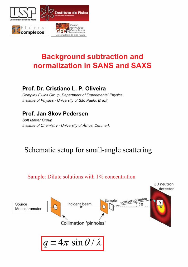
Background subtraction and normalization in SANS and SAXS

Prof. Dr. Cristiano L. P. OliveiraComplex Fluids Group, Department of Experimental PhysicsInstitute of Physics - University of São Paulo, Brazil

Prof. Jan Skov PedersenSoft Matter GroupInstitute of Chemistry - University of Århus, Denmark

Schematic setup for small-angle scattering

Sample: Dilute solutions with 1% concentration

��� /sin4�q

q2�

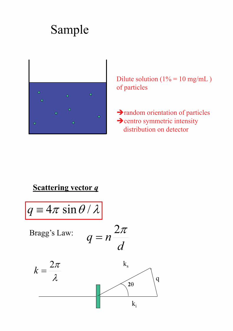
Sample

Dilute solution (1% = 10 mg/mL )of particles

�random orientation of particles�centro symmetric intensity

distribution on detector

Scattering vector q

��� /sin4�q

dnq �2

�Bragg’s Law:

2�

ki

ks

q��2

�k

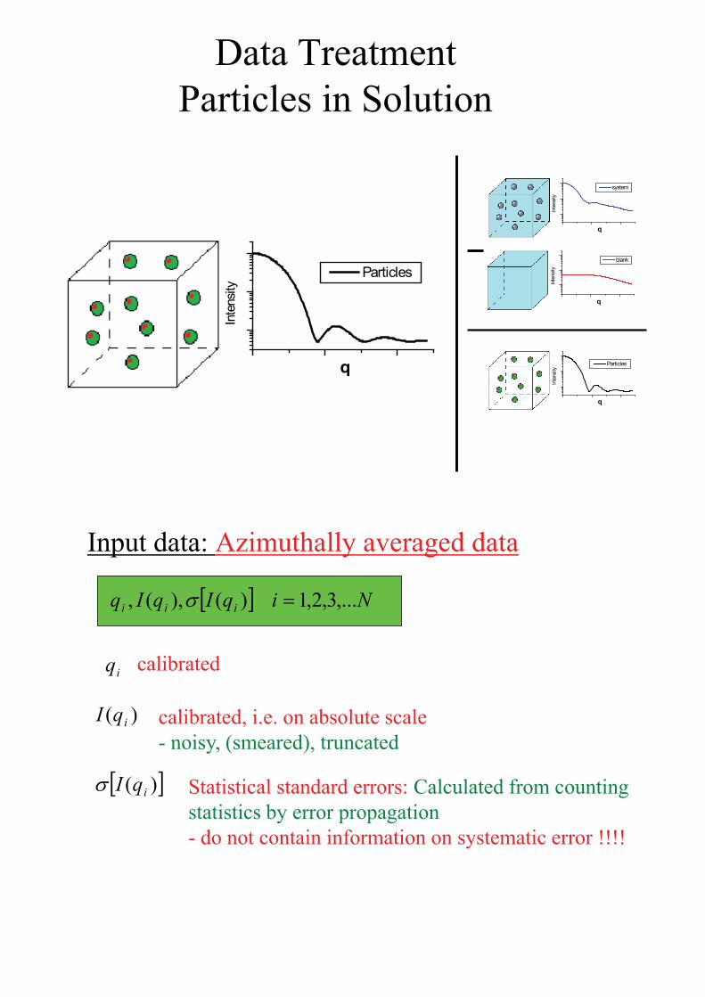
Data TreatmentParticles in Solution

Inte

nsity

q

system

Inte

nsity

q

blank

Inte

nsity

q

Particles

Inte

nsity

q

Particles

Inte

nsity

q

blank

Inte

nsity

q

system

Input data: Azimuthally averaged data

� � NiqIqIq iii ,...3,2,1)(),(, �

)( iqI

� �)( iqI

iq calibrated

calibrated, i.e. on absolute scale - noisy, (smeared), truncated

Statistical standard errors: Calculated from countingstatistics by error propagation- do not contain information on systematic error !!!!

Intensity and Differential Scattering Cross Section

number of scattered neutrons or photons per unit time, relative to the incident flux of neutron or photons, per unit solid angle at q per unit volume of the sample.

)()( qddqI

�

Unit : cm-1

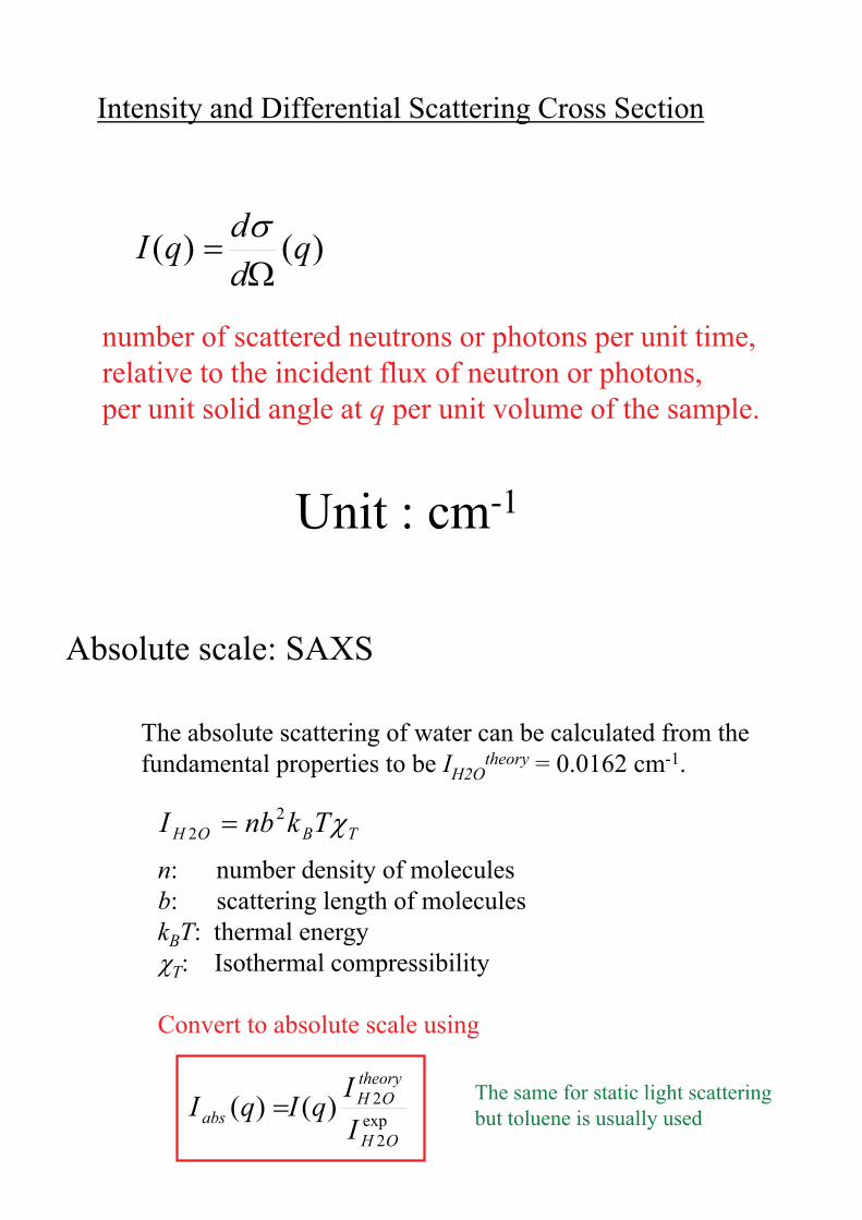
Absolute scale: SAXS

exp2

2)()(OH

theoryOH

abs II

qIqI �

The absolute scattering of water can be calculated from the fundamental properties to be IH2O

theory = 0.0162 cm-1.

TBOH TknbI �22 �

n: number density of moleculesb: scattering length of moleculeskBT: thermal energy�T: Isothermal compressibility

Convert to absolute scale using

The same for static light scatteringbut toluene is usually used

Absolute scale: SANS

exp2

2)()(OH

theoryOH

abs II

qIqI �

neutron and hydrogen parallel spins scatter very different from anti-parallel spins !

Random distribution -> incoherent scattering

)(4/)1(''2 �� gTI theory

OH ��

)(�g is an empirical factor -varies with instrument and detector-include corrections for inelactic effects anf multiple scattering

1. SAXS NT (Bruker AXS) flood correctionspatial correctionazimuthal averaging(beamcenter)(distance calibration Ag-behenate)

2. Home-written software (SUPERSAXS package)conversion, inclusion of meta dataplotbackground subtractionnormalization (H2O)rebinningscaling…

SAXS data processing

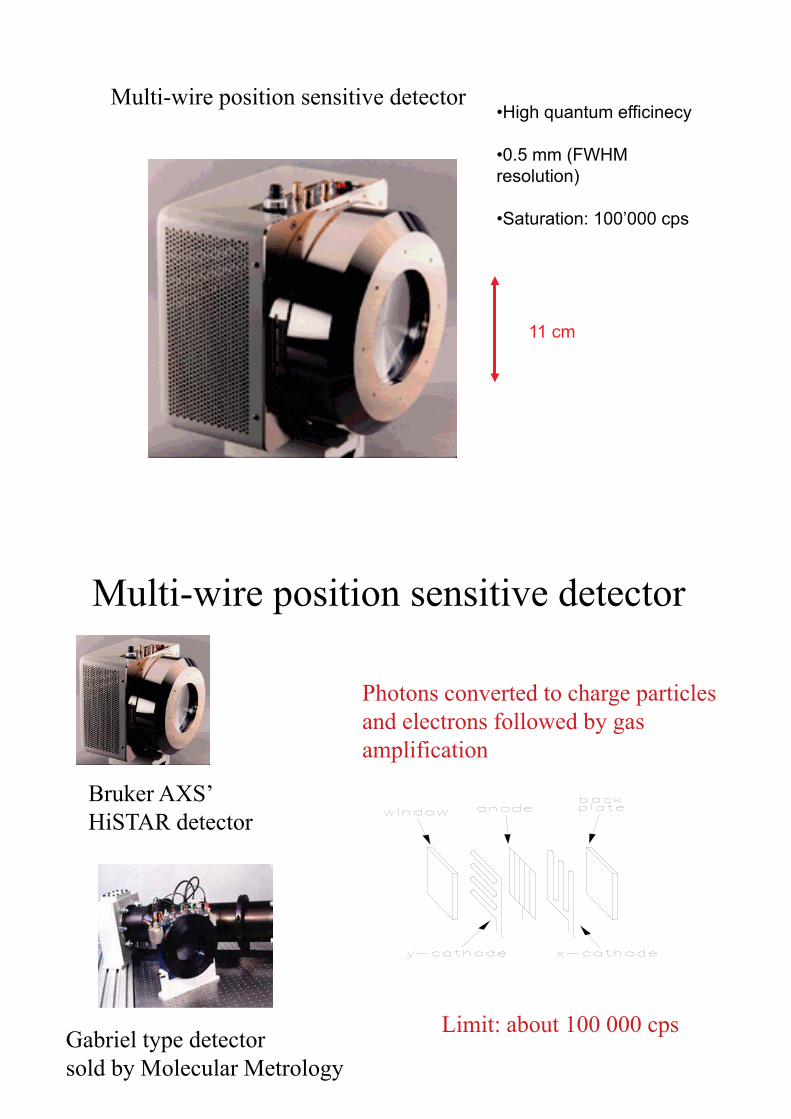
Multi-wire position sensitive detector

11 cm

•High quantum efficinecy

•0.5 mm (FWHM resolution)

•Saturation: 100’000 cps

Multi-wire position sensitive detector

Bruker AXS’ HiSTAR detector

Photons converted to charge particlesand electrons followed by gas amplification

Gabriel type detector sold by Molecular Metrology

Limit: about 100 000 cps

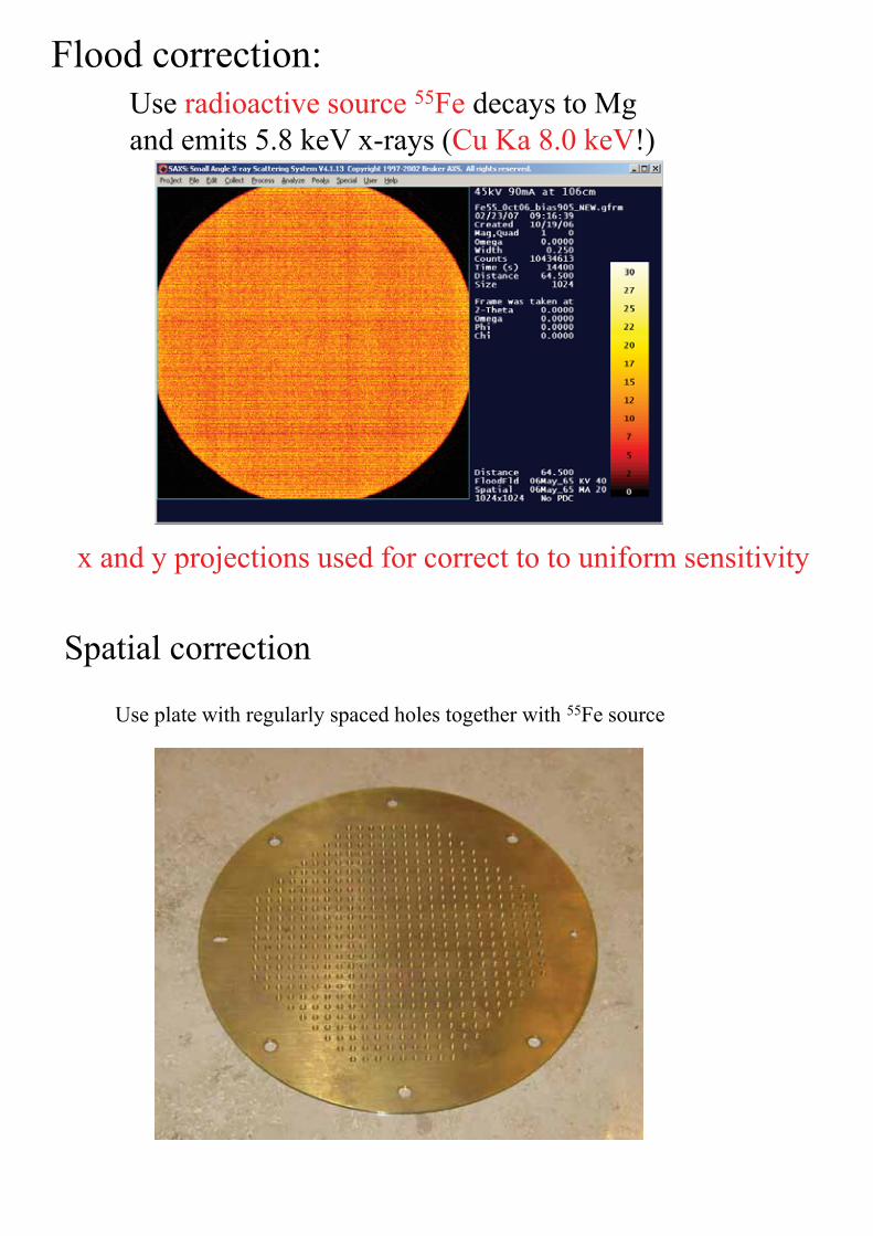
Flood correction: Use radioactive source 55Fe decays to Mg and emits 5.8 keV x-rays (Cu Ka 8.0 keV!)

x and y projections used for correct to to uniform sensitivity

Spatial correction

Use plate with regularly spaced holes together with 55Fe source

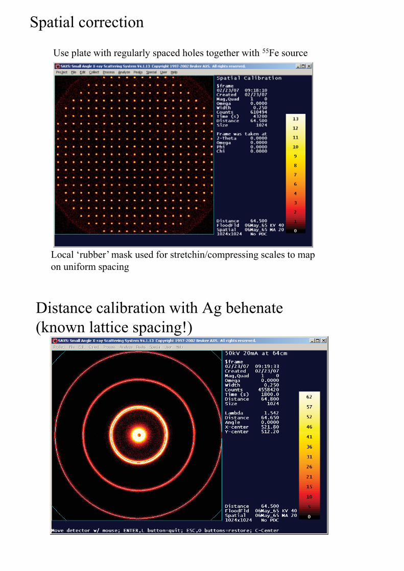
Spatial correction

Use plate with regularly spaced holes together with 55Fe source

Local ‘rubber’ mask used for stretchin/compressing scales to map on uniform spacing

Distance calibration with Ag behenate(known lattice spacing!)

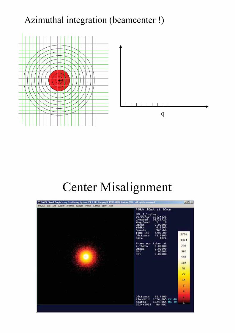
Azimuthal integration (beamcenter !)

q

+

Center Misalignment

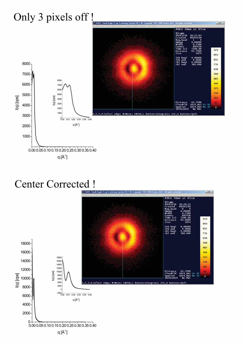
Only 3 pixels off !

0.00 0.05 0.10 0.15 0.20 0.25 0.30 0.35 0.40

1000

2000

3000

4000

5000

6000

7000

8000

0.00 0.01 0.02 0.03 0.04 0.050

1000

2000

3000

4000

5000

6000

7000

8000

I(q) [

cps]

q [Å-1]

q [Å-1]

I(q)

[cps

]

Center Corrected !

0.00 0.05 0.10 0.15 0.20 0.25 0.30 0.35 0.400

2000

4000

6000

8000

10000

12000

14000

16000

18000

0.00 0.01 0.02 0.03 0.04 0.05-2000

02000400060008000

1000012000140001600018000

I(q) [

cps]

q [Å-1]

q [Å-1]

I(q)

[cps

]

0.00 0.01 0.02 0.03 0.04 0.050

5000

10000

15000

20000I(q

) [cp

s]

q [Å-1]

Center OK Center OFF

Raw format: comment lines, then: theta, I, sig(I),q

!@!!GADDS PLOTSO FILE: Chi integration type!@!!Title: 45kV 90mA at 64cm!@!!Frame: $frame!@!!Wavelengths 1.54184 1.54056 1.54439!@!!Integration range: 2Theta: 0.100 to 4.800 Gamma: -180.000 to 180.000!@!!Integration method: bin normalized!@!N!@!SS!@!M!@!L 0.0 0.0 0.0 0.0!@!XDegrees!@!YCounts0.10 38.333706 1.547870 0.0071120.12 100.568771 2.288812 0.0085350.14 182.932983 2.857968 0.0099570.16 233.431747 3.019857 0.0113800.18 242.650208 2.902801 0.0128020.20 234.392487 2.706550 0.0142250.22 224.673691 2.526560 0.0156470.24 218.917648 2.387832 0.0170700.26 210.772476 2.251053 0.0184920.28 204.949387 2.138994 0.0199150.30 202.736664 2.055254 0.0213370.32 194.081619 1.947061 0.0227600.34 189.383942 1.865945 0.024182

Theta,I,sig(I),q

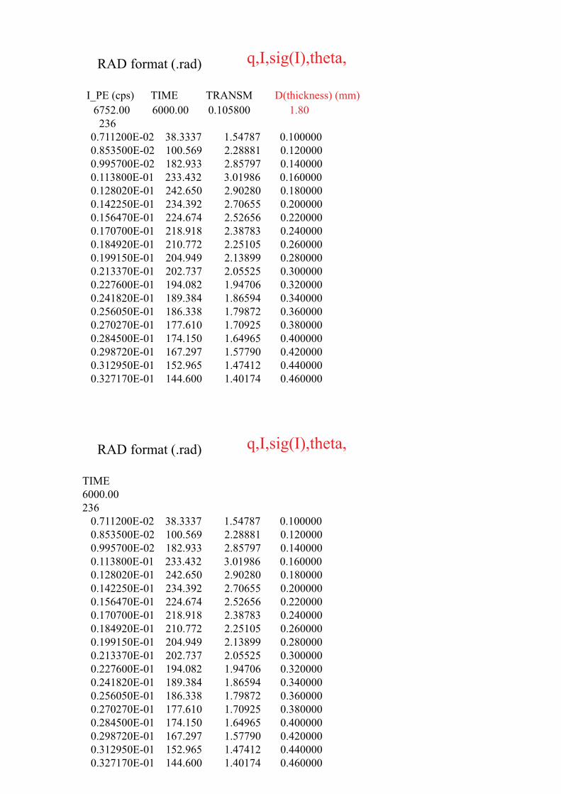
RAD format (.rad)

I_PE (cps) TIME TRANSM D(thickness) (mm)6752.00 6000.00 0.105800 1.80236

0.711200E-02 38.3337 1.54787 0.100000 0.853500E-02 100.569 2.28881 0.120000 0.995700E-02 182.933 2.85797 0.140000 0.113800E-01 233.432 3.01986 0.160000 0.128020E-01 242.650 2.90280 0.180000 0.142250E-01 234.392 2.70655 0.200000 0.156470E-01 224.674 2.52656 0.220000 0.170700E-01 218.918 2.38783 0.240000 0.184920E-01 210.772 2.25105 0.260000 0.199150E-01 204.949 2.13899 0.280000 0.213370E-01 202.737 2.05525 0.300000 0.227600E-01 194.082 1.94706 0.320000 0.241820E-01 189.384 1.86594 0.340000 0.256050E-01 186.338 1.79872 0.360000 0.270270E-01 177.610 1.70925 0.380000 0.284500E-01 174.150 1.64965 0.400000 0.298720E-01 167.297 1.57790 0.420000 0.312950E-01 152.965 1.47412 0.440000 0.327170E-01 144.600 1.40174 0.460000

q,I,sig(I),theta,

RAD format (.rad)

TIME 6000.00 236

0.711200E-02 38.3337 1.54787 0.100000 0.853500E-02 100.569 2.28881 0.120000 0.995700E-02 182.933 2.85797 0.140000 0.113800E-01 233.432 3.01986 0.160000 0.128020E-01 242.650 2.90280 0.180000 0.142250E-01 234.392 2.70655 0.200000 0.156470E-01 224.674 2.52656 0.220000 0.170700E-01 218.918 2.38783 0.240000 0.184920E-01 210.772 2.25105 0.260000 0.199150E-01 204.949 2.13899 0.280000 0.213370E-01 202.737 2.05525 0.300000 0.227600E-01 194.082 1.94706 0.320000 0.241820E-01 189.384 1.86594 0.340000 0.256050E-01 186.338 1.79872 0.360000 0.270270E-01 177.610 1.70925 0.380000 0.284500E-01 174.150 1.64965 0.400000 0.298720E-01 167.297 1.57790 0.420000 0.312950E-01 152.965 1.47412 0.440000 0.327170E-01 144.600 1.40174 0.460000

q,I,sig(I),theta,

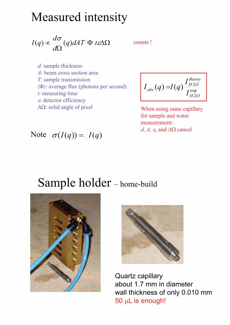
Measured intensity

�

� � tdATqddqI )()(

d: sample thicknessA: beam cross section areaT: sample transmission���: average flux (photons per second)t: measuring time�: detector efficiency ��solid angle of pixel

counts !

Note )())(( qIqI �

exp2

2)()(OH

theoryOH

abs II

qIqI �

When using same capillary for sample and water measurement: d, A, �, and cancel

Sample holder – home-build

Quartz capillaryabout 1.7 mm in diameter wall thickness of only 0.010 mm50 �L is enough!

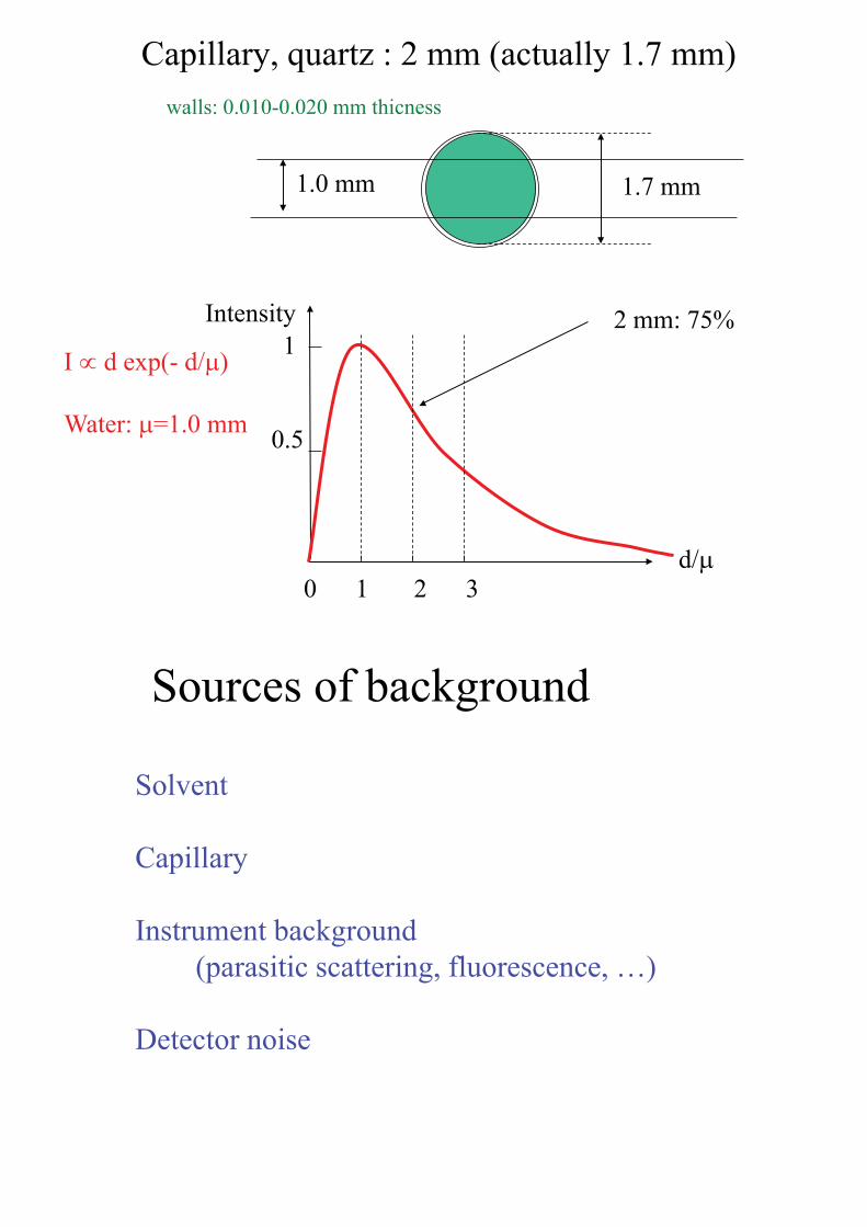
Capillary, quartz : 2 mm (actually 1.7 mm)

d/�

Intensity

0 1 2 3

1

0.5

2 mm: 75%

1.0 mm 1.7 mm

I � d exp(- d/�)

Water: �=1.0 mm

walls: 0.010-0.020 mm thicness

Sources of background

Solvent

Capillary

Instrument background (parasitic scattering, fluorescence, …)

Detector noise

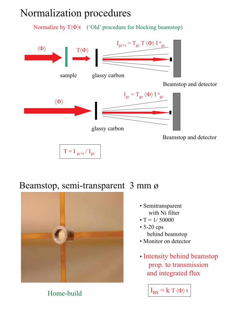
Normalization proceduresNormalize by T���t (‘Old’ procedure for blocking beamstop)

sample

��� T���

glassy carbonBeamstop and detector

Igc+s = Tgc T ��� I ngc

���

glassy carbonBeamstop and detector

Igc = Tgc ��� I ngc

T = I gc+s / Igc

Beamstop, semi-transparent 3 mm ø

• Semitransparentwith Ni filter

• T = 1/ 50000• 5-20 cps

behind beamstop• Monitor on detector

• Intensity behind beamstopprop. to transmission

and integrated flux

IBS = k T ��� tHome-build

Raw data

q [Å-1]

0.0 0.1 0.2 0.3 0.4

I(q)

0

2000

4000

6000

8000

10000

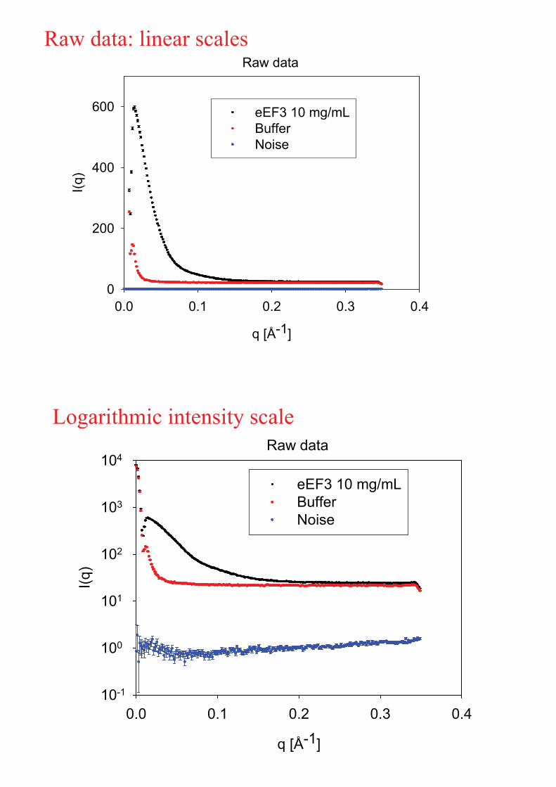
eEF3 10 mg/mLBufferNoise

Raw data

q [Å-1]

0.00 0.01 0.02 0.03 0.04 0.05

I(q)

0

2000

4000

6000

8000

10000

eEF3 10 mg/mLBufferNoise

Raw data

q [Å-1]

0.0 0.1 0.2 0.3 0.4

I(q)

0

200

400

600 eEF3 10 mg/mLBufferNoise

Raw data: linear scales

Raw data

q [Å-1]

0.0 0.1 0.2 0.3 0.4

I(q)

10-1

100

101

102

103

104

eEF3 10 mg/mLBufferNoise

Logarithmic intensity scale

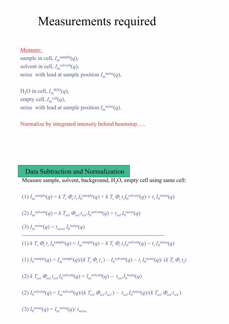
Measure: sample in cell, Im

sample(q), solvent in cell, Im

solvent(q), noise with lead at sample position Im

noise(q),

H2O in cell, ImH2O(q),

empty cell, Imcell(q),

noise with lead at sample position Imnoise(q).

Normalize by integrated intensity behind beamstop…..

Measurements required

Data Subtraction and NormalizationMeasure sample, solvent, background, H2O, empty cell using same cell:

(1) Imsample(q) = k Ts �s ts I0

sample(q) + k Ts �s tsI0solvent(q) + ts I0

noise(q)

(2) Imsolvent(q) = k Tsol �sol tsol I0

solvent(q) + tsol I0noise(q)

(3) Imnoise(q) = tnoise I0

noise(q)---------------------------------------------------------------------------(1) k Ts �s ts I0

sample(q) = Imsample(q) � k Ts �s tsI0

solvent(q) � ts I0noise(q)

(1) I0sample(q) = Im

sample(q)/(k Ts �s ts ) � I0solvent(q) � ts I0

noise(q)/ (k Ts �s ts)

(2) k Tsol �sol tsol I0solvent(q) = Im

solvent(q) � tsol I0noise(q)

(2) I0solvent(q) = Im

solvent(q)/(k Tsol �sol tsol ) � tsol I0noise(q)/(k Tsol �sol tsol )

(3) I0noise(q) = Im

noise(q)/ tnoise

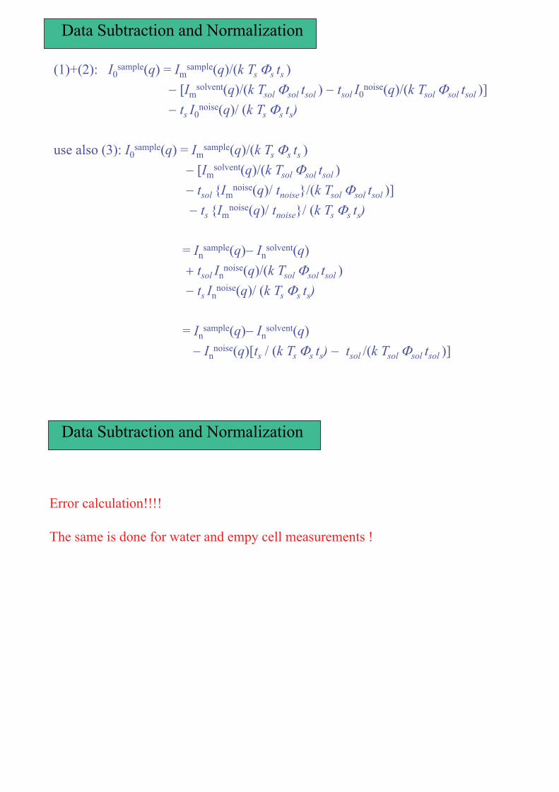
Data Subtraction and Normalization

(1)+(2): I0sample(q) = Im

sample(q)/(k Ts �s ts )� �Im

solvent(q)/(k Tsol �sol tsol ) � tsol I0noise(q)/(k Tsol �sol tsol )]

� ts I0noise(q)/ (k Ts �s ts)

use also (3): I0sample(q) = Im

sample(q)/(k Ts �s ts )� �Im

solvent(q)/(k Tsol �sol tsol )� tsol {Im

noise(q)/ tnoise}/(k Tsol �sol tsol )]� ts {Im

noise(q)/ tnoise}/ (k Ts �s ts)

= Insample(q)� In

solvent(q)� tsol In

noise(q)/(k Tsol �sol tsol )� ts In

noise(q)/ (k Ts �s ts)

= Insample(q)� In

solvent(q)� In

noise(q)[ts / (k Ts �s ts) � tsol /(k Tsol �sol tsol )]

Data Subtraction and Normalization

Error calculation!!!!

The same is done for water and empy cell measurements !

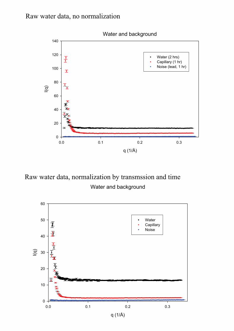
Raw water data, no normalization

Water and background

q (1/Å)

0.0 0.1 0.2 0.3

I(q)

0

20

40

60

80

100

120

140

Water (2 hrs)Capillary (1 hr)Noise (lead, 1 hr)

Raw water data, normalization by transmssion and time

2 hrs accumulationtime

Water and background

q (1/Å)

0.0 0.1 0.2 0.3

I(q)

0

10

20

30

40

50

60

WaterCapillaryNoise

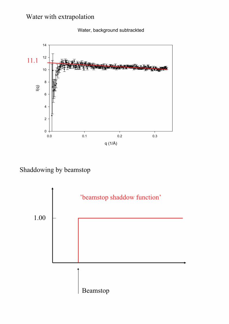
Water with extrapolation

Water, background subtrackted

q (1/Å)

0.0 0.1 0.2 0.3

I(q)

0

2

4

6

8

10

12

14

11.1

Shaddowing by beamstop

Beamstop

1.00

’beamstop shaddow function’

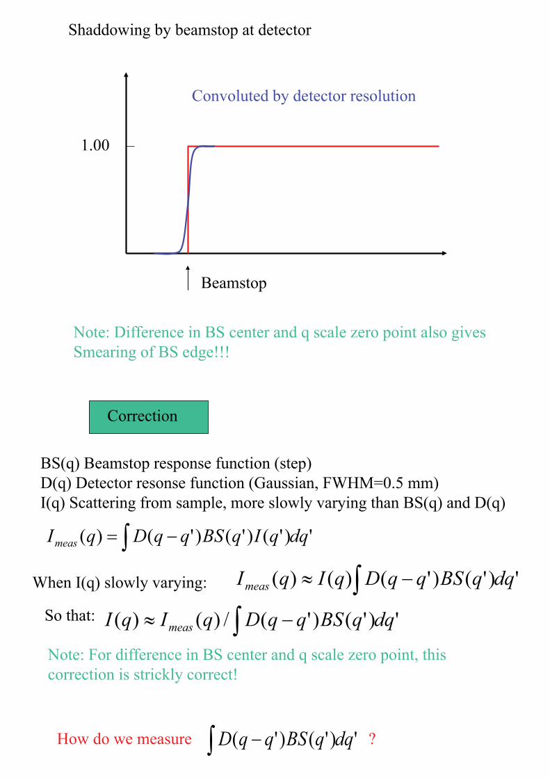
Shaddowing by beamstop at detector

Beamstop

1.00

Convoluted by detector resolution

Note: Difference in BS center and q scale zero point also gives Smearing of BS edge!!!

Correction

BS(q) Beamstop response function (step)D(q) Detector resonse function (Gaussian, FWHM=0.5 mm)I(q) Scattering from sample, more slowly varying than BS(q) and D(q)

')'()'()'()( dqqIqBSqqDqImeas � ��

When I(q) slowly varying: ')'()'()()( dqqBSqqDqIqImeas � ��

')'()'(/)()( dqqBSqqDqIqI meas � ��So that:

How do we measure ? ')'()'( dqqBSqqD� �

Note: For difference in BS center and q scale zero point, this correction is strickly correct!

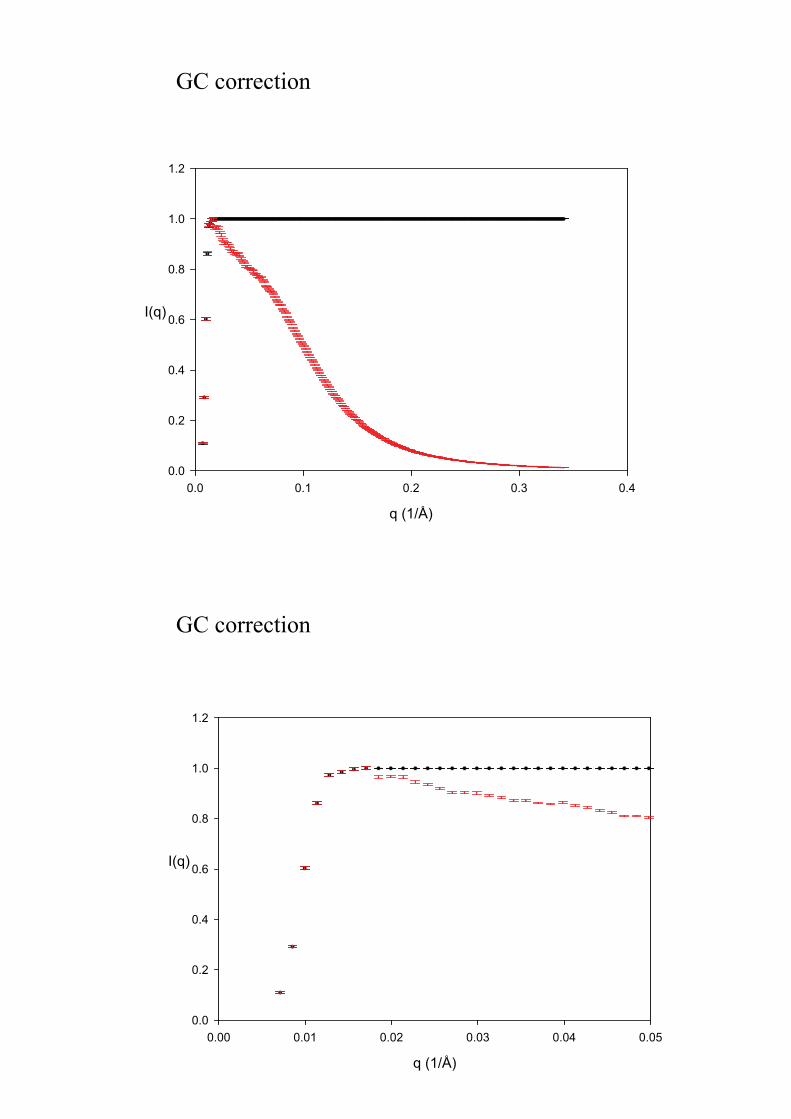
GC correction

q (1/Å)

0.0 0.1 0.2 0.3 0.4

I(q)

0.0

0.2

0.4

0.6

0.8

1.0

1.2

GC correction

q (1/Å)

0.00 0.01 0.02 0.03 0.04 0.05

I(q)

0.0

0.2

0.4

0.6

0.8

1.0

1.2

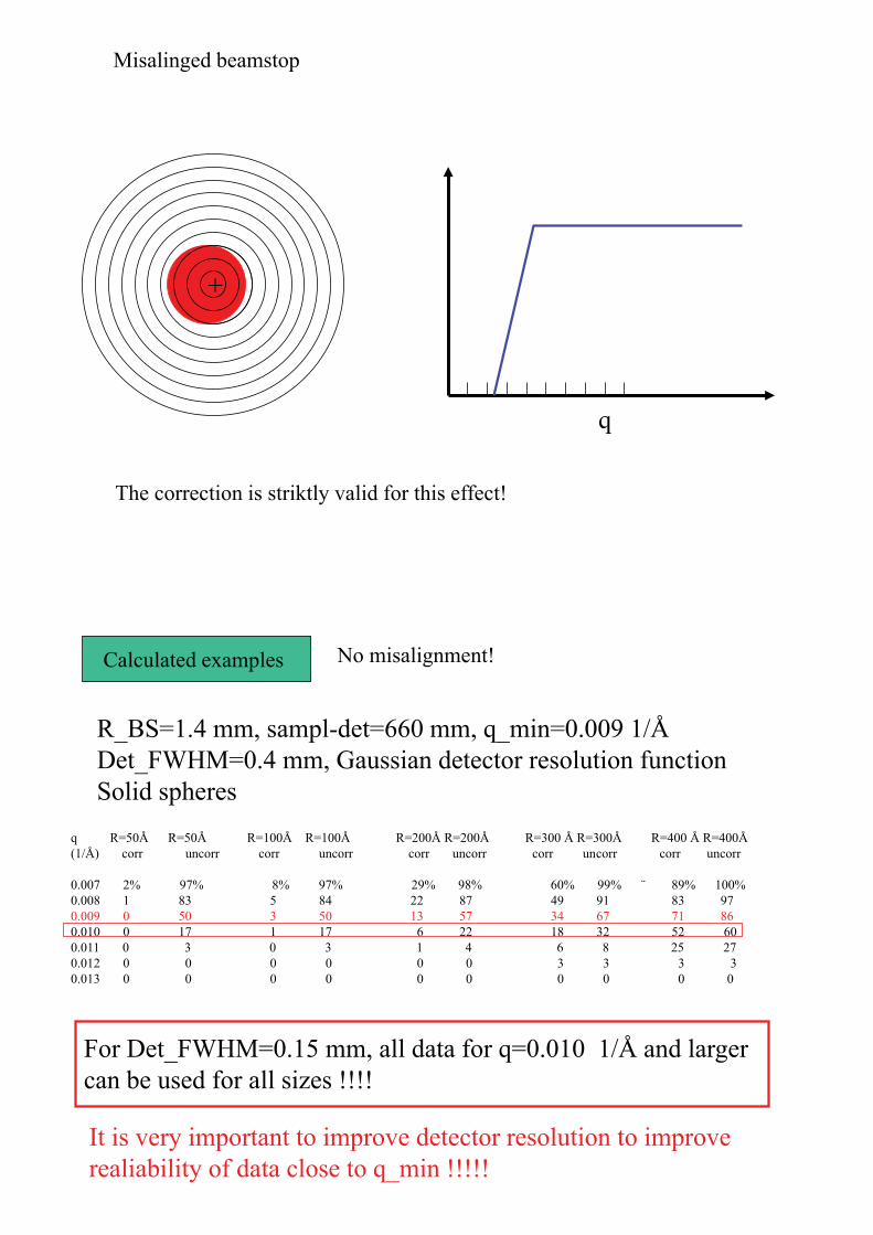
Misalinged beamstop

q

+

The correction is striktly valid for this effect!

Calculated examples

R_BS=1.4 mm, sampl-det=660 mm, q_min=0.009 1/ÅDet_FWHM=0.4 mm, Gaussian detector resolution functionSolid spheres

It is very important to improve detector resolution to improve realiability of data close to q_min !!!!!

q R=50Å R=50Å R=100Å R=100Å R=200Å R=200Å R=300 Å R=300Å R=400 Å R=400Å (1/Å) corr uncorr corr uncorr corr uncorr corr uncorr corr uncorr

0.007 2% 97% 8% 97% 29% 98% 60% 99% ¨ 89% 100% 0.008 1 83 5 84 22 87 49 91 83 970.009 0 50 3 50 13 57 34 67 71 860.010 0 17 1 17 6 22 18 32 52 600.011 0 3 0 3 1 4 6 8 25 270.012 0 0 0 0 0 0 3 3 3 30.013 0 0 0 0 0 0 0 0 0 0

For Det_FWHM=0.15 mm, all data for q=0.010 1/Å and larger can be used for all sizes !!!!

No misalignment!

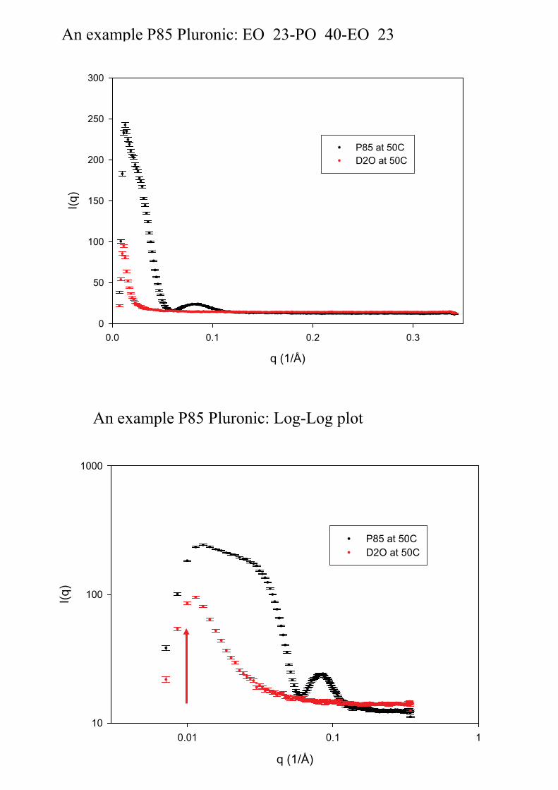
An example P85 Pluronic: EO_23-PO_40-EO_23

q (1/Å)

0.0 0.1 0.2 0.3

I(q)

0

50

100

150

200

250

300

P85 at 50CD2O at 50C

An example P85 Pluronic: Log-Log plot

q (1/Å)

0.01 0.1 1

I(q)

10

100

1000

P85 at 50CD2O at 50C

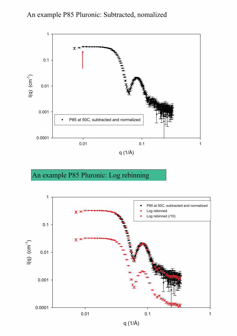
An example P85 Pluronic: Subtracted, nomalized

q (1/Å)

0.01 0.1 1

I(q)

(cm

-1)

0.0001

0.001

0.01

0.1

1

P85 at 50C, subtracted and normalized

An example P85 Pluronic: Log rebinning

q (1/Å)

0.01 0.1 1

I(q)

(cm

-1)

0.0001

0.001

0.01

0.1

1

P85 at 50C, subtracted and normalizedLog rebinnedLog rebinned (/10)

Summary

• Principles of •calibration•background subtraction •Absolute normalization

• Now to SuperSAXS program package

S_U_P_E_R_S_A_X_SPROGRAM PACKAGE FOR DATA TREATMENT, ANALYSIS AND MODELING

Cristiano L P Oliveira

Jan Skov Pedersen

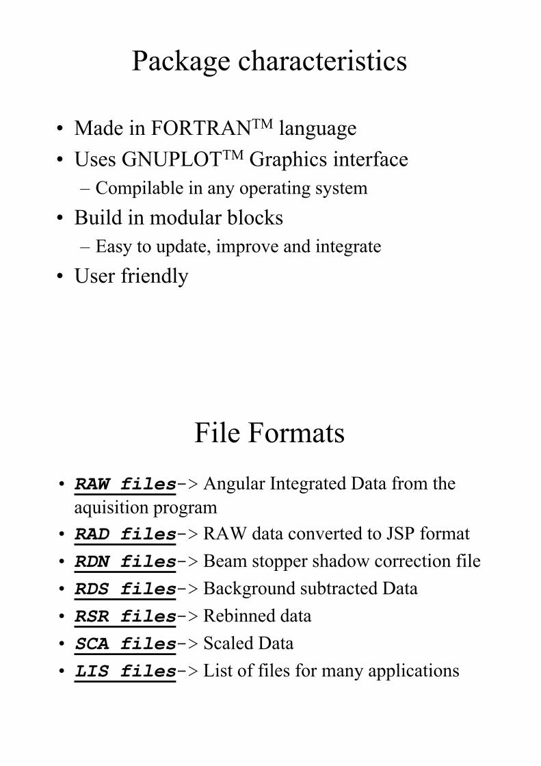
Package characteristics

• Made in FORTRANTM language• Uses GNUPLOTTM Graphics interface

– Compilable in any operating system• Build in modular blocks

– Easy to update, improve and integrate• User friendly

File Formats• RAW files-> Angular Integrated Data from the

aquisition program• RAD files-> RAW data converted to JSP format• RDN files-> Beam stopper shadow correction file• RDS files-> Background subtracted Data• RSR files-> Rebinned data• SCA files-> Scaled Data• LIS files-> List of files for many applications

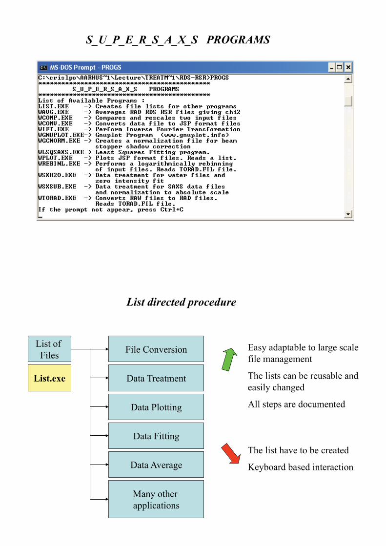
S_U_P_E_R_S_A_X_S PROGRAMS

List of Files

List directed procedure

File Conversion

Data Treatment

Data Plotting

Data Fitting

Data Average

Many other applications

Easy adaptable to large scale file management

The lists can be reusable and easily changed

All steps are documented

The list have to be created

Keyboard based interaction

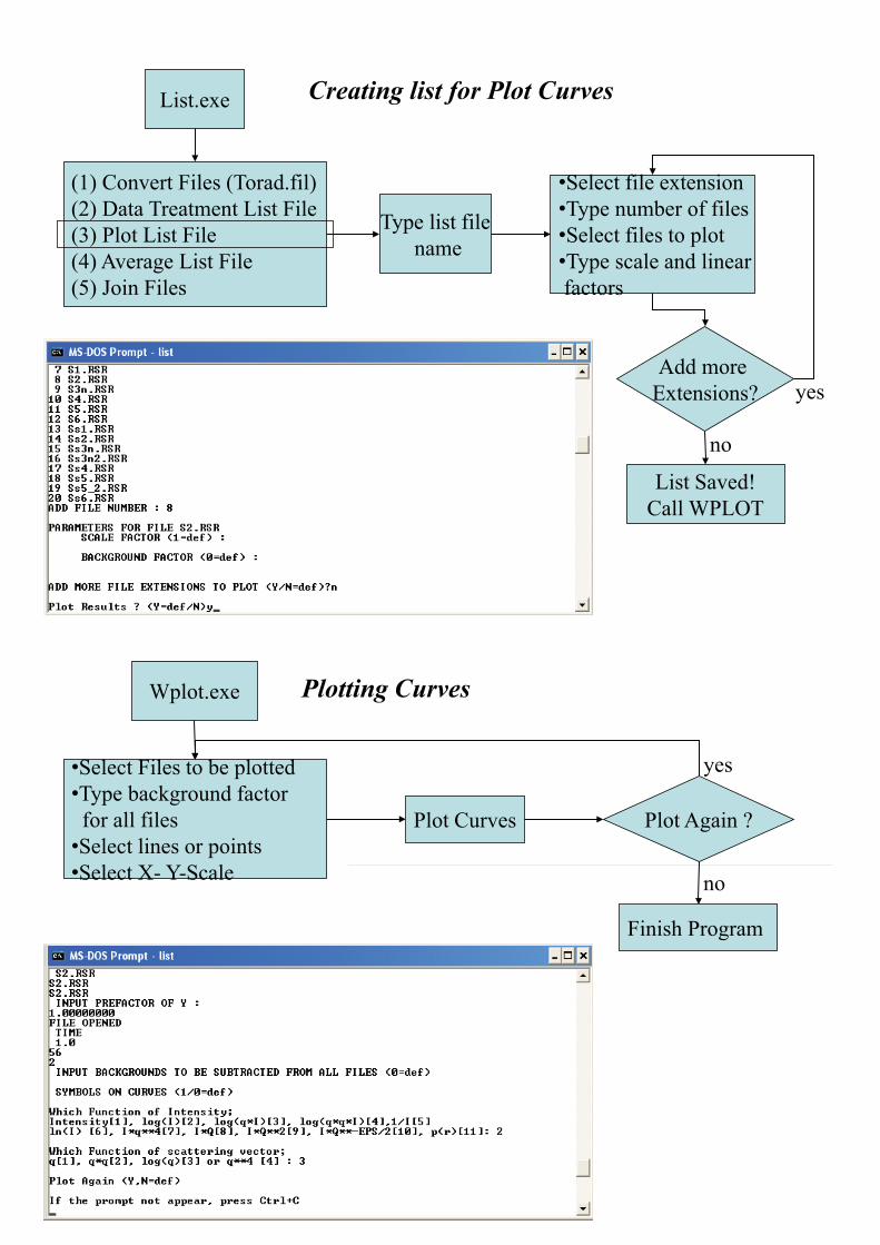
List.exe

List.exe

(1) Convert Files (Torad.fil)(2) Data Treatment List File(3) Plot List File(4) Average List File(5) Join Files

Type files extensionSelect desired files

List Saved!Call WTORAD

Converting from RAW format to RAD format

Read TORAD.FILType aquisition time

for each file

Select file index instead of type the

file name

Data Treatment of SAXS Data

•I(q) is the measured (integrated) scattering intensities

•� is the intensity incident beam

•T is the sample transmission

• t is the exposition time

• (q) is the statistical error of each point.

•Ishadow(q) , shadow (q) are the normalized intensity and error for the beam stopper shadow correction

� � � �� �

� � � �� �

2/1

2

22

2

21

.. ��

�

�

��

�

���

����

�

��qIq

tAqI

qIqq

shadow

shadow

sss

sample

shadowtreated

� � � � � � � �2

2221 .

1.1. ��

�

����

�

��

���bbss

noisebacksample AAqqqq

� � � � � � � �� � � � � � Cwater

Cwater

shadowbbssnoise

noise

bbb

back

sss

sampleTreated I

ddqITTt

qItT

qItTqI

qIº20,

º20,

0/1

......!

"#

$%&

'���

����

���

��

��

�

Bevington (1992), Data Reduction and Error Analysis for the Physical Sciences

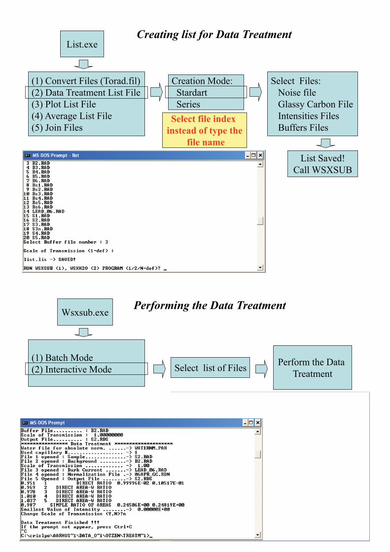
List.exe

(1) Convert Files (Torad.fil)(2) Data Treatment List File(3) Plot List File(4) Average List File(5) Join Files

Select Files:Noise fileGlassy Carbon FileIntensities FilesBuffers Files

List Saved!Call WSXSUB

Creating list for Data Treatment

Creation Mode:Stardart Series

Select file index instead of type the

file name

Wsxsub.exe

(1) Batch Mode(2) Interactive Mode Select list of Files Perform the Data

Treatment

Performing the Data Treatment

Normalized Intensity

Normalized Background

Final Intensity Normalized to Absolute Scale

0.00 0.05 0.10 0.15 0.20 0.25 0.30 0.350.00

0.01

0.02

0.03

0.04

0.05

0.06

0.07

0.08

Experimental Data

I(q) [

cm-1

]

q[Å- 1]

Fast decay

Flat Region

0.00 0.05 0.10 0.15 0.20 0.25 0.30 0.350.00

0.01

0.02

0.03

0.04

0.05

0.06

0.07

0.08

Exp. Data Linear Rebinning

I(q) [

cm-1

]

q[Å- 1]

Data Rebinning

0.00 0.05 0.10 0.15 0.20 0.25 0.30 0.35

1E-3

0.01

0.1

Exp. Data Linear Rebinning 4 points

I(q) [

cm-1

]

q[Å- 1]0.01 0.1

1E-3

0.01

0.1

Exp. Data Linear Rebinning 4 points

I(q) [

cm-1]

q[Å- 1]

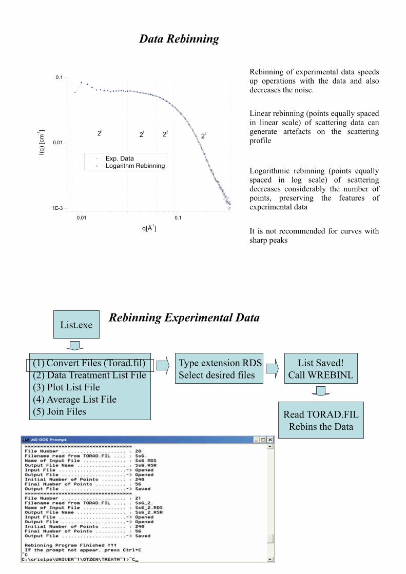
Rebinning of experimental data speedsup operations with the data and alsodecreases the noise.

Linear rebinning (points equally spacedin linear scale) of scattering data cangenerate artefacts on the scatteringprofile

Logarithmic rebinning (points equallyspaced in log scale) of scatteringdecreases considerably the number ofpoints, preserving the features ofexperimental data

It is not recommended for curves withsharp peaks

0.01 0.1

1E-3

0.01

0.1

232221

I(q) [

cm-1]

q[Å- 1]

Exp. Data

20

0.01 0.1

1E-3

0.01

0.1

232221

I(q) [

cm-1]

q[Å- 1]

Exp. Data Logarithm Rebinning

20

List.exe

(1) Convert Files (Torad.fil)(2) Data Treatment List File(3) Plot List File(4) Average List File(5) Join Files

Type extension RDSSelect desired files

List Saved!Call WREBINL

Rebinning Experimental Data

Read TORAD.FILRebins the Data

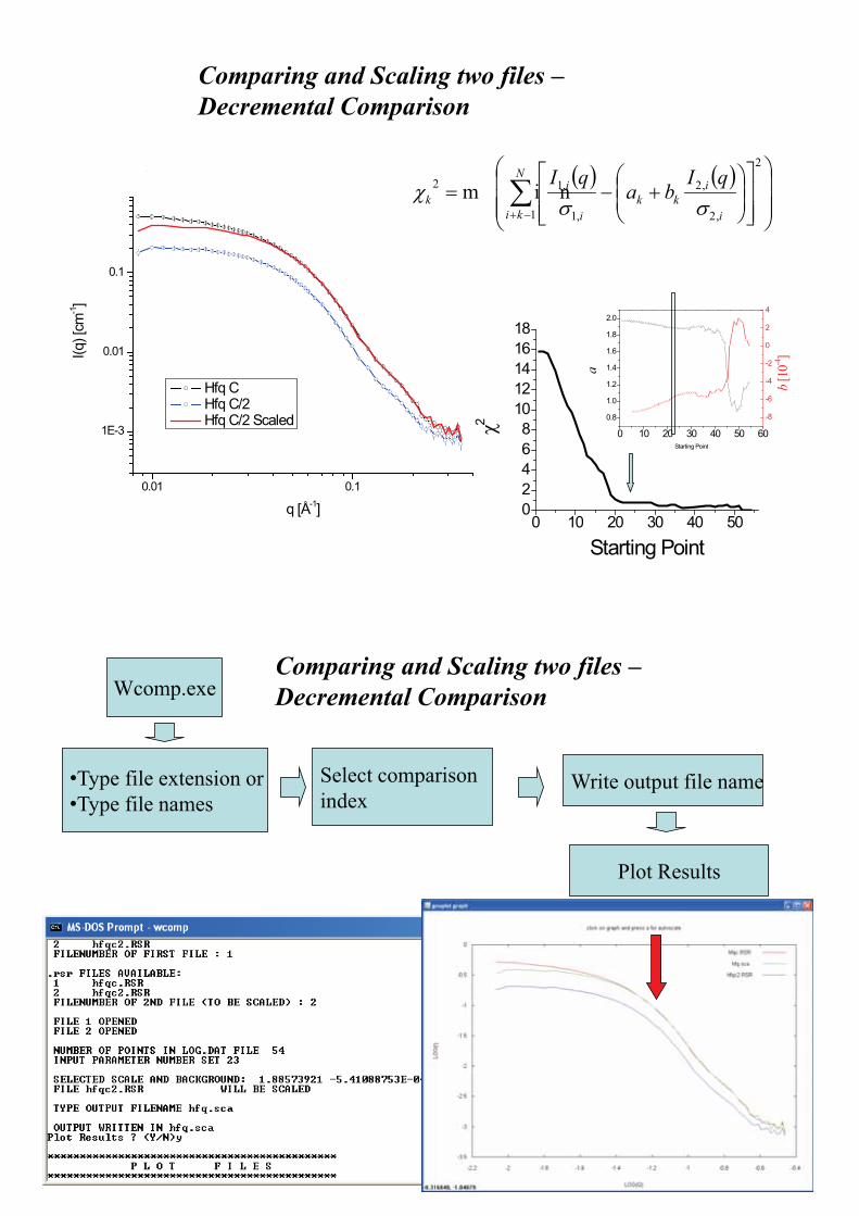
Comparing and Scaling two files –Decremental Comparison

0.01 0.1

1E-3

0.01

0.1

I(q) [

cm-1]

q [Å-1]

Hfq C Hfq C/2

0 10 20 30 40 50 60

0.8

1.0

1.2

1.4

1.6

1.8

2.0

-8

-6

-4

-2

0

2

4

a

Starting Point

b [1

0-4]

0

�12

�22

0.01 0.1

1E-3

0.01

0.1

I(q) [

cm-1]

q [Å-1]

Hfq C Hfq C/2 Hfq C/2 Scaled

� � � ����

�

�

���

�

""#

$

%%&

'���

����

��� (

��

N

ki i

ikk

i

ik

qIba

qI

1

2

,2

,2

,1

,12 m i n

�

0 10 20 30 40 5002468

1012141618

�2

Starting Point

Wcomp.exe

•Type file extension or•Type file names

Write output file name

Comparing and Scaling two files –Decremental Comparison

Select comparison index

Plot Results

List.exe

(1) Convert Files (Torad.fil)(2) Data Treatment List File(3) Plot List File(4) Average List File(5) Join Files

•Select file extension•Type number of files•Select files to plot•Type scale and linear factors

List Saved!Call WPLOT

Creating list for Plot Curves

Type list filename

Add more Extensions? yes

no

Wplot.exe

•Select Files to be plotted•Type background factor for all files

•Select lines or points•Select X- Y-Scale

Plot Curves

Plotting Curves

Plot Again ?

yes

Finish Program

no

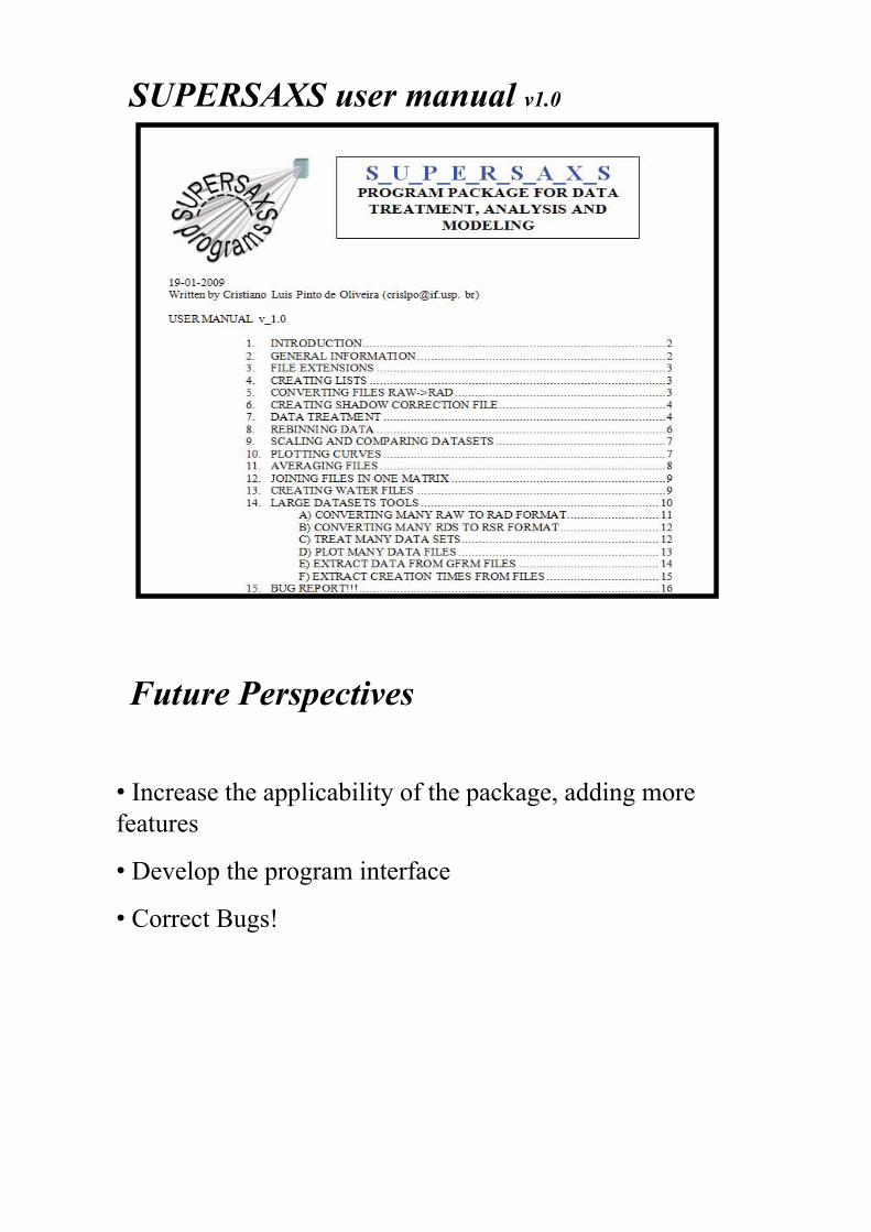
SUPERSAXS user manual v1.0

Future Perspectives

• Increase the applicability of the package, adding more features

• Develop the program interface

• Correct Bugs!