Embed Size (px)
DESCRIPTION
baker
Citation preview
CHAPTER III
MARKET REALISM: CURRENCY PRICING AND THE GAINS
FROM TRADE BETWEEN COUNTRIES AT DIFFERENT LEVELS
OF POLITICAL DEVELOPMENT
Chapter 1 introduced the foundations for the neoliberal interpretation of interna-
tional institutions’ advocacy of liberalized trade. A critical assumption behind the
neoliberal perspective is that free markets are in the collective interest – that is, that
liberalized trade maximizes the gains to world as a whole, without regard to how
those gains might be distributed. The economic theory underpinning this belief was
reviewed in Chapter 2, “Economics and Interest,” where I also noted that the prin-
cipal challenges to laissez-faire economics have concerned distributional issues, not
market liberals’ claim that perfectly free markets lead to the optimal use of resources.
In this chapter, I present a model that calls this latter belief into question. While the
classic arguments upon which free market liberalism is founded involve barter models
of trade, I introduce differentially risky currencies, and derive two important results.
First, consumers in countries with the riskier currency pay higher prices in perfectly
free markets than those with less risky currencies, shrinking their share of world out-
put. Second, currency traders’ aversion to risky currencies introduces an endogenous
distortion into perfectly free markets that leaves the equilibrium suboptimal from
the perspective of the collective interest. The chapter begins with a review of the
62
63
nuts and bolts of the standard general equilibrium model. In the middle section, I
introduce currencies. First I demonstrate that the barter results do not change when
risk-free currencies are introduced; then I derive the results described by allowing
the currencies to be differentially risky. In the final section, I provide a discussion of
appropriate interventions.
The standard barter model
For most westerners, the suggestion that unfettered markets are efficient has at-
tained the status of “well-known fact”; the proof, however, is unfamiliar. In broad
outline, it follows the logic discussed in Chapter 2. Prices producers are willing to
accept are still determined by the cost of the inputs they use in production, akin to
Smith’s “natural price.” Input costs, though, are no longer tied to the amount of
labor embodied in the inputs. Rather, they are determined indirectly by the utility
consumers attach to the various goods that can be produced by them. The argu-
ment, then, is composed of three pieces. The first piece describes the behavior of a
utility-maximizing consumer, and derives a relationship between his utility function
and the rate at which he will be willing to exchange two goods (that is, the barter
price – in the illustration that follows, the number of coffee beans he will pay for
an M&M). The second piece describes the behavior of profit-maximizing producers.
The critical result here is that when producers are producing as much of two goods
as they can, the price they’re willing to accept is related to the relative amounts
of inputs required to produce each of the two products. The third piece combines
the two pieces of information about price for the final result. If the barter price is
related, through consumer behavior, to the consumer’s relative utilities for the two
goods; and it is related, through producer behavior, to the relative input costs of
the two goods; then the relative input costs of the two goods must be related to the
consumer’s relative utilities for them. More precisely, the market mechanism – the
64
interaction of producer and consumer incentives – allocates inputs in such a way that
out of all combinations of two goods that can be produced from a given set of inputs,
the combination that will be produced is the one that consumers will be happiest
with.
With no intervention
Formally, consider two representative agents, Susan and Pedro, residing in two
different countries. Both subsist on coffee and M&M’s. Susan’s country has a com-
parative advantage in M&M production, Pedro’s has a comparative advantage in the
production of coffee. For clarity of exposition, complete specialization is assumed.1
Assume that both are rational utility maximizers with identical utility functions.
Both like M&M’s and coffee, but enjoy each additional cup of coffee and hand-
ful of M&M’s a little less than the last one consumed – that is, their common
utility function U(.) is assumed to be increasing in M&M and coffee consumption
(∂U/∂Cmm > 0, ∂U/∂Ccf > 0) but concave(∂2U/∂C2
mm < 0, ∂2U/∂C2cf < 0
). Addi-
tionally, it is assumed to be twice differentiable. Pedro, then, will trade coffee for
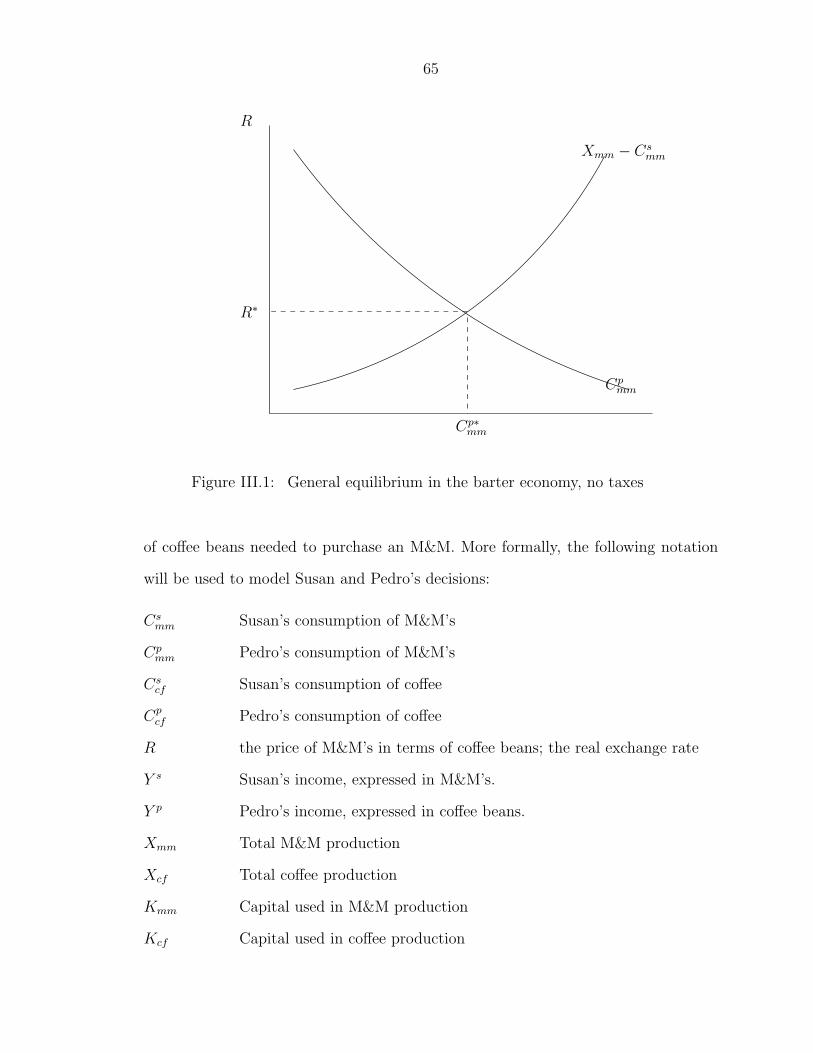
some of Susan’s M&M’s A model of their exchange, viewed from Pedro’s perspective,
is presented in Figure III.1. The barter price is expressed in terms of the number
of coffee beans Pedro pays for each M&M. The downward sloping demand curve
represents the number of M&M’s he is willing to buy at different price levels; the
upward-sloping supply curve represents the quantity of M&M’s that Susan is willing
to supply at different prices. In equilibrium, Pedro buys Cp∗mm M&M’s from Susan in
exchange for a quantity of coffee beans that will become her final coffee consumption,
Cs∗cf . The ratio of these two quantities is the equilibrium barter price, R∗, the number
1 Allowing for incomplete specialization (the more general case) does not change the results atall; it merely adds the requirement that we keep track of four goods – Susan’s M&M’s and coffeeproduced by Susan, and M&M’s and coffee produced by Pedro – instead of two.
65
Cpmm
R∗
R
Xmm − Csmm
Cp∗mm
Figure III.1: General equilibrium in the barter economy, no taxes
of coffee beans needed to purchase an M&M. More formally, the following notation
will be used to model Susan and Pedro’s decisions:
Csmm Susan’s consumption of M&M’s
Cpmm Pedro’s consumption of M&M’s
Cscf Susan’s consumption of coffee
Cpcf Pedro’s consumption of coffee
R the price of M&M’s in terms of coffee beans; the real exchange rate
Y s Susan’s income, expressed in M&M’s.
Y p Pedro’s income, expressed in coffee beans.
Xmm Total M&M production
Xcf Total coffee production
Kmm Capital used in M&M production
Kcf Capital used in coffee production
66
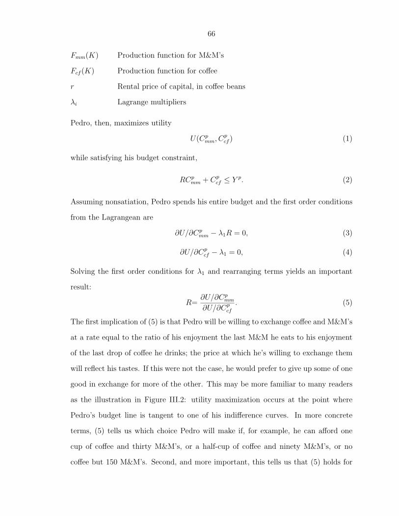
Fmm(K) Production function for M&M’s
Fcf (K) Production function for coffee
r Rental price of capital, in coffee beans
λi Lagrange multipliers
Pedro, then, maximizes utility
U(Cpmm, Cp
cf ) (1)
while satisfying his budget constraint,
RCpmm + Cp
cf ≤ Y p. (2)
Assuming nonsatiation, Pedro spends his entire budget and the first order conditions
from the Lagrangean are
∂U/∂Cpmm − λ1R = 0, (3)
∂U/∂Cpcf − λ1 = 0, (4)
Solving the first order conditions for λ1 and rearranging terms yields an important
result:
R=∂U/∂Cp
mm
∂U/∂Cpcf
. (5)
The first implication of (5) is that Pedro will be willing to exchange coffee and M&M’s
at a rate equal to the ratio of his enjoyment the last M&M he eats to his enjoyment
of the last drop of coffee he drinks; the price at which he’s willing to exchange them
will reflect his tastes. If this were not the case, he would prefer to give up some of one
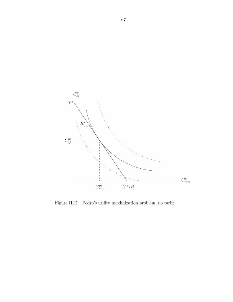
good in exchange for more of the other. This may be more familiar to many readers
as the illustration in Figure III.2: utility maximization occurs at the point where
Pedro’s budget line is tangent to one of his indifference curves. In more concrete
terms, (5) tells us which choice Pedro will make if, for example, he can afford one
cup of coffee and thirty M&M’s, or a half-cup of coffee and ninety M&M’s, or no
coffee but 150 M&M’s. Second, and more important, this tells us that (5) holds for
67
Y p/R
R∗
Cpcf
Y p
Cp∗cf
Cpmm
Cp∗mm
Figure III.2: Pedro’s utility maximization problem, no tariff
68
the demand functions Cpmm(R, Y ) and Cp
cf (R, Y ) derived from Pedro’s maximization
problem. Since prices and output will be determined by the interaction of supply
and demand, (5) enters into the determination of the relative prices of the two goods,
therefore into how much of each good will be produced, and so finally, into the
determination of how much of the capital stock will be allocated to M&M production
and how much to coffee production. To see this, turn now to the supply side. To
keep things as simple as possible, without any loss of generality, Susan and Pedro
are assumed to supply labor costlessly, but pay r coffee beans for each unit of capital
consumed. Susan maximizes profits
RXmm − rKmm, (6)
subject to the production function
Xmm ≤ Fmm(Kmm). (7)
Assuming she produces as much as she can, the first order conditions yield
R =r
∂Fmm/∂Kmm
(8)
At the same time, Pedro maximizes profits
Xcf − rKcf (9)
subject to the constraint
Xcf ≤ Fcf (Kcf ) (10)
Assuming he also produces as much as he can, the first order conditions of his maxi-
mization problem yield
r =∂Fcf
∂Kcf
(11)
Substituting (11) into (8),
R =∂Fcf/∂Kcf
∂Fmm/∂Kmm
. (12)
69
(12) tells us that producers will behave in such a way that the barter price is equal to
the marginal rate of transformation – metaphorically, the rate at which coffee beans
could be “unpicked” to the bushes they were taken from, and the recovered capital
could be reallocated to M&M production. More concretely, (12) tells us that profit-
maximizing producers will charge prices that reflect the costs of the inputs they use
in production. Equating (5) and (12),
∂U/∂Cpmm
∂U/∂Cpcf
=∂Fcf/∂Kcf
∂Fmm/∂Kmm
: (13)
the marginal rate of substitution is equal to the marginal rate of transformation.
When prices serve to equate the marginal rate of transformation with the marginal
rate of substitution, no combination of goods can be produced from the factor inputs
that would be valued more highly than the current combination. In other words, the
price mechanism acts as an invisible hand ensuring that factors are put to best use.
The barter model with a tax
Now consider what happens if Pedro’s government places a tariff on M&M imports.
He still maximizes U(Cmm, Ccf ) as in the previous analysis, but if we let t be the tariff
rate, his budget constraint becomes
R(1 + t)Cpmm + Cp
cf ≤ Y p. (2′)
Only the second first-order condition changes. (3) still holds, (4) becomes
∂U/∂Cpmm − λ2R(1 + t) = 0. (4′)
and (5) is now
R =1
1 + t
∂U/∂Cpmm
∂U/∂Cpcf
(5′).
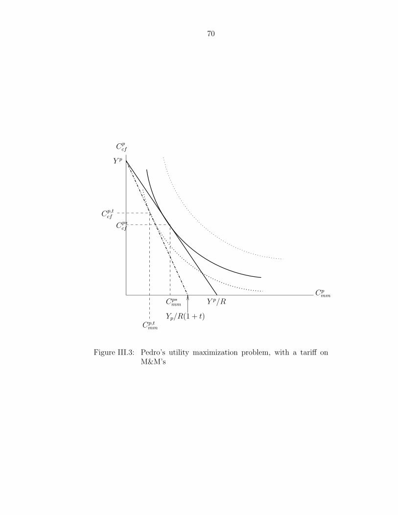
This introduces two problems. The first is the obvious one: Pedro is able to buy less
coffee. As seen in Figure III.3, his consumption bundle is now on a lower indifference
70
Yp/R(1 + t)
Cpcf
Y p
Cp,tcf
Cp∗cf
Cp∗mm Y p/R
Cp,tmm
Cpmm
Figure III.3: Pedro’s utility maximization problem, with a tariff onM&M’s
71
curve; he is clearly worse off. The second problem is more subtle. Imagine that
we could give Pedro enough additional income so that he could reach his pre-tariff
utility level after the tariff has been applied. This can be represented graphically by
shifting the new budget line outward, until it touches the pre-tariff indifference curve
but is still parallel to the tariffed budget line. The additional compensation would
allow Pedro to purchase a combination of coffee and M&M’s that makes him just as
happy as the pre-tariff combination, but they are not the same consumption bundle.
Because the tariff necessitates that he forego more coffee beans for each M&M, the
bundle purchased with his income and the additional compensation will include more
coffee and fewer M&M’s than the bundle he purchased before the tariff. His choice, in
other words, no longer reflects the relative input cost of the two goods. (13) becomes
1
1 + t
∂U/∂Cpmm
∂U/∂Cpcf
=∂Fcf/∂Kcf
∂Fmm/∂Kmm
(13′).
The marginal rate of substitution is no longer equated with the marginal rate of
transformation. The price distortion introduced by the tariff has broken the link
between them, and as a result, production inputs are no longer put to their best use.
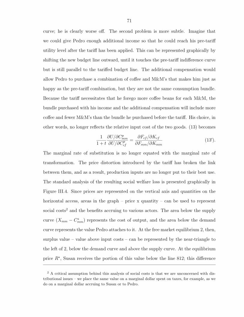
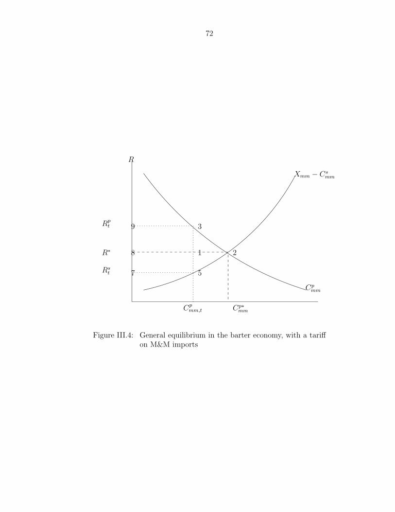
The standard analysis of the resulting social welfare loss is presented graphically in
Figure III.4. Since prices are represented on the vertical axis and quantities on the
horizontal access, areas in the graph – price x quantity – can be used to represent
social costs2 and the benefits accruing to various actors. The area below the supply
curve (Xmm − Csmm) represents the cost of output, and the area below the demand
curve represents the value Pedro attaches to it. At the free market equilibrium 2, then,
surplus value – value above input costs – can be represented by the near-triangle to
the left of 2, below the demand curve and above the supply curve. At the equilibrium
price R∗, Susan receives the portion of this value below the line 812; this difference
2 A critical assumption behind this analysis of social costs is that we are unconcerned with dis-tributional issues – we place the same value on a marginal dollar spent on taxes, for example, as wedo on a marginal dollar accruing to Susan or to Pedro.
72
Cpmm
R
R∗ 2
3
5
18
9
7
Xmm − Csmm
Rpt
Rst
Cpmm,t Cp∗
mm
Figure III.4: General equilibrium in the barter economy, with a tariffon M&M imports
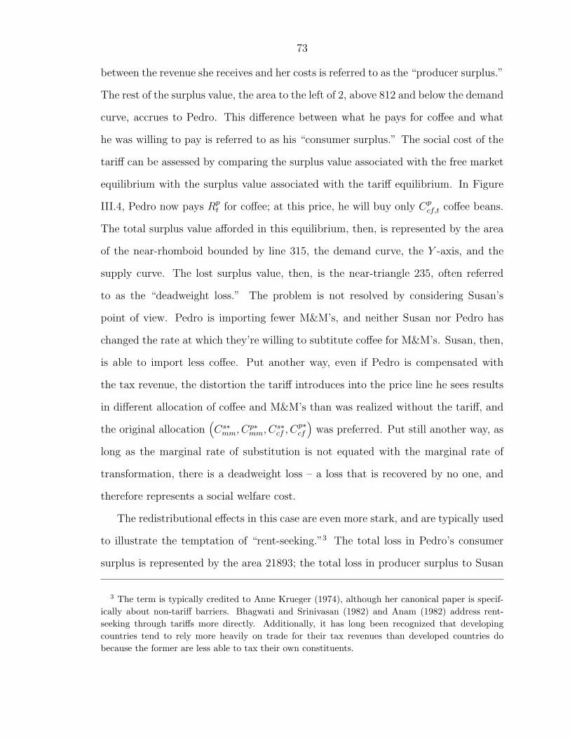
73
between the revenue she receives and her costs is referred to as the “producer surplus.”
The rest of the surplus value, the area to the left of 2, above 812 and below the demand
curve, accrues to Pedro. This difference between what he pays for coffee and what
he was willing to pay is referred to as his “consumer surplus.” The social cost of the
tariff can be assessed by comparing the surplus value associated with the free market
equilibrium with the surplus value associated with the tariff equilibrium. In Figure
III.4, Pedro now pays Rpt for coffee; at this price, he will buy only Cp
cf,t coffee beans.
The total surplus value afforded in this equilibrium, then, is represented by the area
of the near-rhomboid bounded by line 315, the demand curve, the Y -axis, and the
supply curve. The lost surplus value, then, is the near-triangle 235, often referred
to as the “deadweight loss.” The problem is not resolved by considering Susan’s
point of view. Pedro is importing fewer M&M’s, and neither Susan nor Pedro has
changed the rate at which they’re willing to subtitute coffee for M&M’s. Susan, then,
is able to import less coffee. Put another way, even if Pedro is compensated with
the tax revenue, the distortion the tariff introduces into the price line he sees results
in different allocation of coffee and M&M’s than was realized without the tariff, and
the original allocation(Cs∗
mm, Cp∗mm, Cs∗
cf , Cp∗cf
)was preferred. Put still another way, as
long as the marginal rate of substitution is not equated with the marginal rate of
transformation, there is a deadweight loss – a loss that is recovered by no one, and
therefore represents a social welfare cost.
The redistributional effects in this case are even more stark, and are typically used
to illustrate the temptation of “rent-seeking.”3 The total loss in Pedro’s consumer
surplus is represented by the area 21893; the total loss in producer surplus to Susan
3 The term is typically credited to Anne Krueger (1974), although her canonical paper is specif-ically about non-tariff barriers. Bhagwati and Srinivasan (1982) and Anam (1982) address rent-seeking through tariffs more directly. Additionally, it has long been recognized that developingcountries tend to rely more heavily on trade for their tax revenues than developed countries dobecause the former are less able to tax their own constituents.
74
is represented by the area 21875. The tax revenue, though, is represented by the
rectangle 9357. Assuming that the tax revenue accrues to Pedro, his net loss in
consumer surplus is the near-triangle 123, but he gains a portion of what Susan had
been receiving as producer surplus, 8157. In other words, Susan bears more than the
total of the social cost, and Pedro comes out ahead. In the following section, I will
show that currency risk premiums introduce a distortion that has a similar effect.
While the incidence is not the same as that for the tax on Susan’s coffee imports, the
risk premium still serves to drive a wedge between the marginal rate of substitution
and the marginal rate of transformation that moves the equilibrium away from the
efficient equilibrium.
Add currencies
Now suppose that money is used for transactions in both economies. Dollars($)
are used in Susan’s country, while pesos(℘) are used in Pedro’s. First, some new
terms:
Pmm the price of M&M’s in dollars
Pcf the price of coffee in pesos
S the spot exchange rate, in pesos per dollar.
To make it clear that the distortion is caused by the risk premium and not merely
by the introduction of currencies, the analysis is presented in two parts. In the
first, I show that the desirable free market equilibrium obtains when currencies are
used but since all transactions are simultaneous, riskiness is not an issue. In the
second, I assume that transactions are contracted in advance, and that one currency
is perceived as being riskier than the other.
75
Contemporaneous trade with currencies
In this case, Pedro still maximizes U(Cmm, Ccf ), but his budget constraint becomes
SPmmCpmm + PcfC
pcf ≤ PcfY
p. (2′′′)
The new first order conditions are
∂U/∂Cpmm − λ3SPmm = 0, (3′′′)
∂U/∂Cpcf − λ3Pcf = 0, (4′′′))
When we solve (3′′′) and (4′′′) for λ3, equate the two expressions, and solve for the
exchange rate, we find
S =Pcf
Pmm
∂U/∂Cpmm
∂U/∂Cpcf
. (5′′′)
To evaluate whether or not this is consistent with the maximally efficient allocation,
though, we need an expression involving R, the real exchange rate. Specifically, we
need to derive the relationship between the spot exchange rate S and the barter price
R. In the case of simultaneous transactions, this is straightforward. Money is valued
only for its purchasing power (its function as a store of value is irrelevant), and its
purchasing power is known. It must be the case, then, that
S = RPcf
Pmm
. (14)
Substituting this into (5′′′) yields
R =∂U/∂Cp
mm
∂U/∂Cpcf
, (15)
as in the barter case.
Trade using differentially risky currencies
Suppose, however, that Susan and Pedro must contract in advance for imports.
Then they must set prices and amounts to be exchanged in advance, and secure
76
foreign currency on the forward market. Let Ft,t+1 represent the current price, in
pesos, of dollars delivered in the next period. Pmm and Pcf represent the future prices
contracted in the current period. St+1 represents the future spot exchange rate, and
Et(St+1) is this period’s expectation of next period’s spot rate. I assume that utilities
are constant through time; i.e., that Ut(Cmm,t+1, Ccf,t+1) = Ut+1(Cmm,t+1, Ccf,t+1).
Then Pedro maximizes
Ut(Cmm,t+1, Ccf,t+1) (1′′′′)
while satisfying his budget constraint,
Ft,t+1PmmCpmm,t+1 + PcfC
pcf,t+1 ≤ PcfY
pt+1. (2′′′′)
Assuming nonsatiation, Pedro spends his entire budget and the first order conditions
from the Lagrangean are
∂U/∂Cmm,t+1 − λ4Ft,t+1Pmm = 0, (3′′′′)
∂U/∂Ccf,t+1 − λ4Pcf = 0, (4′′′′)
The demand functions Cpmm,t+1(P, Y p
t+1) and Cpcf,t+1(P, Y p
t+1) can be derived from these
conditions and the budget constraint. In this case, solving the first order conditions
for λ4 and equating gives
Ft,t+1 =Pcf
Pmm
∂U/∂Cpmm
∂U/∂Cpcf
. (5′′′′)
If the forward rate Ft,t+1 were equal to the realized spot rate, St+1, the solution
would be the same as in previous case where all exchanges are contemporaneous.
Empirically, this tends not to be the case, though. There is an extensive literature
documenting bias in forward exchange rates.4 The bias is commonly interpreted as
a risk premium: unlike the case of simultaneous exchanges, money’s role as a store
4 Hodrick (1987), Levich (1985), Lewis (1995) and Engel (1996) provide extensive surveys. Thesubject is addressed in more detail in Chapter 4.
77
of value comes into play, and some currencies are perceived as being more trustwor-
thy than others. The relevance of political factors for currency risk premiums has
been argued in MacDonald and Taylor (1991), Baker (1997) and Christodoulakis and
Kalyvitis (1997), and has been demonstrated empirically in Bachman (1992), Bern-
hard and LeBlang (forthcoming, AJPS 2002) and Freeman (2001).5 In the case of a
currency exchange between developed and developing countries, we might expect cur-
rency traders to view the currency of the less developed country as riskier, in general,
than the currency of the developed country for several reasons. Where economic insti-
tutions are still nascent, future money supplies and convertibility are less predictable
than in countries with longstanding monetary authorities who have established pat-
terns of behavior. Moreover, developing countries are more vulnerable to political
disturbances that affect the trustworthiness of their currencies. In extreme cases, the
stability of property rights and enforceability of contracts may be in question. In this
case, suppose Pedro’s currency is perceived to be riskier, as a store of value, than
Susan’s currency, and that both agents are risk-averse. Then the forward rate, Ft,t+1
must exceed the realized spot rate, St+1: Susan will demand a premium for agreeing
to make the future exchange of dollars for pesos that is necessary to complete the
trade. If we let ε represent the risk premium,
Ft,t+1 = St+1 + ε. (16)
We know that by definition,
St+1 = Rt+1Pcf
Pmm
. (14′)
From (5′′′′), (16) and (15′),
Rt+1 =St+1
St+1 + ε
∂U/∂Cpmm,t+1
∂U/∂Cpcf,t+1
(17)
5 To my knowledge, no one has considered the distributional consequences of currency riskpremiums.
78
– a new equation for the real exchange rate. Notice that when the two currencies are
viewed as being equally risky (or riskless), ε = 0 and (17) is identical to equation (5),
the real exchange rate in the barter case. When Pedro’s currency is perceived as being
riskier than Susan’s, however, the risk premium is positive, and the real exchange rate
is less than it is in the barter case. That is, Pedro pays more for Susan’s M&M’s, or
put another way, Susan pays fewer M&M’s for Pedro’s coffee beans. Pedro’s share of
world output, then, drops while Susan’s share increases. Moreover, just as in the case
of a tariff, a wedge has been driven between the marginal rate of substitution and
the marginal rate of transformation. The risk premium introduces an endogenous
distortion that keeps the price mechanism from directing inputs to their best uses, so
the risk premium not only results in a redistribution from Pedro to Susan, but also
results in a social welfare loss.
Welfare-improving alternatives
Jagdish Bhagwati, in his seminal piece on optimal intervention (1971/1987), clas-
sifies trade distortions into four general categories, and describes welfare-improving
policy interventions for each case. His treatment differs from mine in two important
respects. First, he deals only with real-side phenomena (the barter case); distortions
due to the deviation of currency pricing from purchasing power parity are not con-
sidered. Second, he assumes all decisions are contemporaneous. This latter difference
is especially important: the same problem that creates the endogenous distortion I
have described – agents’ inability to predict the future exchange rate – must plague
attempts at optimal intervention. The analysis that follows, then, is intended less
as prescription than as the final piece of the proof that the free market equilibrium
is not the optimal equilibrium, and more important, support for the argument that
many of the policies third world countries follow and/or advocate are consistent not
only with their own interests but with the collective interest.
79
Bhagwati’s advice that optimal interventions should directly address the source of
the distortion has direct implications for capital controls: clearly the most straight-
forward way to eliminate the distortion introduced by currency risk premiums is by
enforcing a forward exchange rate that more closely approximates the realized spot
rate. Developing countries that sell their currencies forward at a premium over the
market rate, then, may be enhancing global welfare by defying the advice of insti-
tutions such as the IMF. Second best interventions are those described by Bhagwati
for cases where, as he describes them, “DRS 6=DRT=FRT” – a wedge has been driven
between the marginal rate of substitution and the marginal rate of transformation.
In this case, either subsidizing Pedro’s M&M consumption or taxing Susan’s coffee
consumption will offset the distortion introduced by the risk premium. Proofs follow.
Subsidizing M&M consumption
Assume that conditions are the same as those described in the section “Trade with
differentially risky currencies,” except that Pedro’s M&M consumption is subsidized
at rate 1/(1+b). Intuitively, the subsidy offsets the risk premium he pays for importing
M&M’s.
His utility function remains the same, but his budget constraint becomes
(1/1 + b)Ft,t+1PmmCpmm + PcfC
pcf ≤ PcfY
p. (2′′′′′)
Assuming nonsatiation, Pedro spends his entire budget and the first order conditions
from the Lagrangean are
∂U
∂Cpmm
− λ51
1 + bFt,t+1Pmm = 0, (3′′′′′)
∂U
∂Cpcf
− λ5Pcf = 0, (4′′′′′)
80
Solving the first order conditions for λ5 and equating gives
Pmm
Pcf
=1 + b
Ft,t+1
∂U/∂Cpmm
∂U/∂Cpcf
; (5′′′′′)
Recalling
St+1 = Rt+1Pcf
Pmm
, (14′)
and
Ft,t+1 = St+1 + ε (16)
(5′′′′′) becomes
Rt+1 =St+1(1 + b)
St+1 + ε
∂U/∂Cpmm
∂U/∂Cpcf
(18)
Clearly, for b = ε/St+1, the subsidy offsets the distortion introduced by the currency
risk premium, the price mechanism acts to equalize the marginal rate of substitution
and the marginal rate of transformation, and so factors are put to best use.
While the subsidy mitigates the effects of the distortion regardless of its source,
to prevent redistribution in favor of Susan, the subsidy must come from her. In other
words, the developing world’s subsidy of third world imports is one intervention that
redresses the distortion introduced by currency risk premium. Considered in this
light, third world demands for a Generalized System of Preferences can be defended
as promoting not just the interests of developing countries, but the collective interest.
Taxing Susan’s coffee consumption
Suppose, instead, that Susan’s coffee consumption is taxed at rate t. Intuitively,
we want to make her refund the risk premium that accrues to her whenever she
converts currency to import coffee. While we have been examining the utility maxi-
mization problem from Pedro’s perspective so far, the logic is the same for Susan.
She maximizes utility
U(Csmm, Cs
cf ), (1′)
81
subject to the budget constraint
PmmCsmm + (1 + t)
1
Ft,t+1
PcfCscf ≤ PmmY s. (2′′′′′′)
Assuming nonsatiation, Susan spends her entire budget and the first order conditions
from the Lagrangean are
∂U/∂Cmm − λ6Pmm = 0, (3′′′′′′)
∂U/∂Ccf − λ61
Ft,t+1
(1 + t)Pcf = 0, (4′′′′′′)
In this case, solving the first order conditions for λ6 and equating gives
Pmm
Pcf
=1 + t
Ft,t+1
∂U/∂Csmm
∂U/∂Cscf
(5′′′′′′)
Again, recalling
St+1 = Rt+1Pmm
Pcf
, (14′)
and
Ft,t+1 = St+1 + ε (16)
(5′′′′′′) becomes
Rt+1 =St+1(1 + t)
St+1 + ε
∂U/∂Csmm
∂U/∂Cscf
(19)
A tax such that t = ε/St+1 offsets the distortion introduced by the currency risk
premium. In other words, it is both in the individual interest of developing countries,
and in the collective interest, for the developed world to pay higher nominal prices
for third world goods than third world consumers are required to pay.
Conclusions
The neoliberal interpretation of international institutions holds that institutions
such as the GATT, its successor the WTO, the IMF, and the World Bank help inter-
national actors reach the mutually cooperative outcome in interactions appropriately
modelled as a prisoner’s dilemma. Intervention in trade has long been considered a
82
textbook example: countries have private incentives, it is argued, to impose tariffs
and other trade barriers. If both countries in a trading pair follow their private in-
terests, though, they reach an outcome that is less desirable both individually and
collectively than the outcome that would have resulted if they had both adhered to
( laissez-faire) trade policies. These beliefs have formed the basis for the developed
world to make market liberalization a chronic condition for loans by the World Bank
and the IMF, and an explicit goal of the GATT and the WTO. These beliefs, however,
are based on barter models of trade, such as the model presented in the first section
of this chapter. They do not take into account the distortion introduced because
currency pricing is affected not only by economic factors, but by traders’ confidence
in governments’ abilities to defend their currencies and to provide the legal infrastruc-
ture necessary for the credibility of contracts. I have shown, first, that when traders
are assumed to contract in advance, and to rely on differentially risky currencies to
conduct transactions, laissez-faire trade policies result in a redistribution from the
country with the least-trusted currency to the country whose currency is perceived
to be less risky. Moreover, laissez-faire trade policies are suboptimal from a social
welfare perspective; policies consistent with those commonly advocated by the de-
veloping world, such as capital controls and preferential pricing favoring developing
countries can actually be welfare-enhancing. The behavior of international economic
institutions, then, is more aptly depicted by the realist perspective: institutions are
means by which the most powerful countries in the international system impose their
preferences on less powerful countries, regardless of the implications for the collective
interest. The argument rests on the assertion that currencies of the developing world
are perceived as being riskier than those of developed countries, a proposition I test in
the following chapter. Moreover, it has testable implications for countries’ preferences
regarding currency controls.