B

Balanced Box Decomposition Tree(Spatial Index)

�Nearest Neighbor Problem

Bayesian Estimation

� Indoor Positioning, Bayesian Methods

Bayesian Inference

�Hurricane Wind Fields, Multivariate Model-ing

Bayesian Maximum Entropy

�Uncertainty, Modeling with Spatial and Tem-poral

Bayesian Network Integrationwith GIS

Daniel P. Ames and Allen AnselmoDepartment of Geosciences, Geospatial SoftwareLab, Idaho State University, Pocatello, ID, USA

Synonyms

Directed acyclic graphs; Influence diagrams;Probabilistic map algebra; Probability networks;Spatial representation of Bayesian networks

Definition

A Bayesian network (BN) is a graphical-mathematical construct used to probabilisticallymodel processes which include interdependentvariables, decisions affecting those variables, andcosts associated with the decisions and statesof the variables. BNs are inherently systemrepresentations and, as such, are often usedto model environmental processes. Becauseof this, there is a natural connection between

© Springer International Publishing AG 2017S. Shekhar et al. (eds.), Encyclopedia of GIS,DOI 10.1007/978-3-319-17885-1

102 Bayesian Network Integration with GIS

certain BNs and GIS. BNs are represented asa directed acyclic graph structure with nodes(representing variables, costs, and decisions) andarcs (directed lines representing conditionallyprobabilistic dependencies between the nodes). ABN can be used for prediction or analysis of real-world problems and complex natural systemswhere statistical correlations can be foundbetween variables or approximated using expertopinion. BNs have a vast array of applicationsfor aiding decision-making in areas such asmedicine, engineering, natural resources, anddecision management. BNs can be used to modelgeospatially interdependent variables as wellas conditional dependencies between geospatiallayers. Additionally, BNs have been found to beuseful and highly efficient in performing imageclassification on remotely sensed data.

Historical Background

Originally described by Pearl (1988), BNs havebeen used extensively in medicine and computerscience (Heckerman 1997). In recent years,BNs have been applied in spatially explicitenvironmental management studies. Examplesinclude the Neuse Estuary Bayesian ecologicalresponse network (Borsuk and Reckhow 2000),Baltic salmon management (Varis and Kuikka1996), climate change impacts on Finnishwatersheds (Kuikka and Varis 1997), the InteriorColumbia Basin Ecosystem Management Project(Lee and Bradshaw 1998), and waterbodyeutrophication (Haas 1998). As illustratedin these studies, a BN graph structures aproblem such that it is visually interpretable bystakeholders and decision-makers while servingas an efficient means for evaluating the probableoutcomes of management decisions on selectedvariables.

Both BNs and GIS can be used to representspatially explicit, probabilistically connectedenvironmental and other systems; however, theintegration of the two techniques has only beenexplored relatively recently. BN integration withGIS typically takes one of the four distinctforms: (1) BN-based layer combination (i.e.,

probabilistic map algebra) as demonstrated inTaylor (2003); (2) BN-based classification asdemonstrated in Stassopoulou et al. (1998)and Stassopoulou et al. (1998); (3) using BNsfor intelligent, spatially oriented data retrieval,as demonstrated in Walker et al. (2004) andWalker et al. (2005); and (4) GIS-based BNdecision support system (DSS) frameworkswhere BN nodes are spatially represented ina GIS framework as presented by Ames et al.(2005).

Scientific Fundamentals

As noted above, BNs are used to model reality byrepresenting conditional probabilistic dependen-cies between interdependent variables, decisions,and outcomes. This section provides an in-depthexplanation of BN analysis using an example BNmodel called the “Umbrella” BN (Fig. 1), an aug-mented version of the well-known “Weather” in-fluence diagram presented by Shachter and Peot(1992). This simple BN attempts to model thevariables and outcomes associated with the de-cision to take or not take an umbrella on agiven outing. This problem is represented in the

A. Forecast B. Weather

C. Take Umbrella D. Satisfaction

Sunny

Cloudy

Take

Do not Take

Rainy

No Rain

Rain

Bayesian Network Integration with GIS, Fig. 1Umbrella Bayesian decision network structure. A and Bnature nodes, C a decision node, and D a utility node

Bayesian Network Integration with GIS 103

B

BN by four nodes. “Weather” and “Forecast”are nature or chance nodes where “Forecast”is conditioned on the state of “Weather” and“Weather” is treated as a random variable witha prior probability distribution based on histor-ical conditions. “Take Umbrella” is a decisionvariable that, together with the “Weather” vari-able, defines the status of “Satisfaction.” The“Satisfaction” node is known as a “Utility” or“Value” node. This node associates a resultantoutcome value (monetary or otherwise) to repre-sent the satisfaction of the individual based onthe decision to take the umbrella and whetheror not there is rain. Each of these BN nodescontains discrete states where each variable staterepresents abstract events, conditions, or numericranges of each variable.

The Umbrella model can be interpreted asfollows: if it is raining, there is a higher prob-ability that the forecast will predict it will rain.In reverse, through the Bayesian network “back-ward propagation of evidence,” if the forecastpredicts rain, it can be inferred that there isa higher chance that rain will actually occur.The link between “Forecast” and “Take Um-brella” indicates that the “Take Umbrella” deci-sion is based largely on the observed forecast.Finally, the link to the “Satisfaction” utility nodefrom both “Take Umbrella” and “Weather” cap-tures the relative gains in satisfaction derivedfrom every combination of states of the BNvariables.

Bayesian networks are governed by two math-ematical techniques: conditional probability andBayes’ theorem.

Conditional probability is defined as the prob-ability of one event given the occurrence of an-other event and can be calculated as the jointprobability of the two events occurring dividedby the probability of the second event:

P.AjB/ DP.A;B/

P.B/: (1)

From Eq. 1, the fundamental rule for proba-bility calculus and the downward propagation ofevidence in a BN can be derived. Specifically, it isseen that the joint probability of A and B equals

the conditional probability of event A given B ,multiplied by the probability of event B (Eq. 2):

P.A;B/ D P.AjB/ � P.B/ : (2)

Equation 2 is used to compute the probabilityof any state in the Bayesian network given thestates of the parent node events. In Eq. 3, theprobability of state Ax occurring given parent Bis the sum of the probabilities of the state of Ax

given state Bi , with i being an index to the statesof B , multiplied by the probability of that stateof B:

P.Ax ; B/ DX

i

P.AxjBi / � P.Bi / : (3)

Similarly, for calculating states with multipleparent nodes, the equation is modified to makethe summation of the conditional probability ofthe state Ax given states Bi and Cj multiplied bythe individual probabilities of Bi and Cj :

P.Ax ; B; C /

DX

i;j

P.AxjBi ; Cj / � P.Bi / � P.Cj / : (4)

Finally, though similar in form, utility nodesdo not calculate probability, but instead calcu-late the utility value as a metric or index giventhe states of its parent or parents as shown inEqs. 5 and 6:

U.A;B/ DX

i

U.AjBi / � P.Bi / (5)

U.A;B;C /

DX

i;j

U.AjBi ; Cj / � P.Bi / � P.Cj / : (6)

The second equation that is critical to BNmodeling is Bayes’ theorem:

P.AjB/ DP.BjA/ � P.A/

P.B/: (7)

104 Bayesian Network Integration with GIS

The conditional probability inversion repre-sented here allows for the powerful techniqueof Bayesian inference, for which BNs are par-ticularly well suited. In the Umbrella model,inferring a higher probability of a rain given arainy forecast is an example application of Bayes’theorem.

Connecting each node in the BN is a condi-tional probability table (CPT). Each nature node(state variable) includes a CPT that stores theprobability distribution for the possible states ofthe variable given every combination of the statesof its parent nodes (if any). These probabilitydistributions can be assigned by frequency anal-ysis of the variables and expert opinion based onobservation or experience, or they can be set tosome “prior” distribution based on observationsof equivalent systems.

Tables 1 and 2 show CPTs for the UmbrellaBN. In Table 1, the probability distribution ofrain is represented as 70% chance of no rain and30% chance of rain. This CPT can be assumedto be derived from historical observations of thefrequency of rain in the given locale. Table 2represents the probability distribution of the pos-sible weather forecasts (“Sunny,” “Cloudy,” or“Rainy”) conditioned on the actual weather event.For example, when it actually rained, the priorforecast called for “Rainy” 60% of the time,“Cloudy” 25% of the time, and “Sunny” 15%of the time. Again, these probabilities can bederived from historical observations of predictionaccuracies or from expert judgment.

Bayesian Network Integration with GIS, Table 1Probability of rain

Weather

No rain Rain

70% 30%

Bayesian Network Integration with GIS, Table 2Forecast probability conditioned on rain

Forcast

Weather Sunny Cloudy Rainy

No rain 70% 20% 10%

Rain 15% 25% 60%

Bayesian Network Integration with GIS, Table 3Satisfaction utility conditioned on rain and the “TakeUmbrella” decision

Satisfaction

Weather Take Umbrella Satisfaction

No Rain Take 20 units

No Rain Do not Take 100 units

Rain Take 70 units

Rain Do not Take 0 units

Table 3 is a utility table defining the relativegains in utility (in terms of generic “units” ofsatisfaction) under all of the possible states ofthe BN. Here, satisfaction is highest when thereis no rain and the umbrella is not taken andlowest when the umbrella is not taken but it doesrain. Satisfaction “units” are in this case assignedas arbitrary ratings from 0 to 100, but in morecomplex systems, utility can be used to representmonetary or other measures.

Following is a brief explanation of the imple-mentation and use of the Umbrella BN. First itis useful to compute P (Forecast D Sunny) givenunknown Weather conditions as follows:

P.Forecast D Sunny/

DX

iDNoRain; Rain

P.Forecast

D SunnyjWeatheri / � P.Weatheri /

D 0:7 � 0:7C 0:15 � 0:3 D 0:535 D 54%:

Next P (Forecast D Cloudy) and P (ForecastD Rainy) can be computed as

P.Forecast D Cloudy; Weather/

D 0:2 � 0:7C 0:25 � 0:3 D 0:215 D 22%

P.Forecast D Cloudy; Weather/

D 0:1 � 0:7C 0:6 � 0:3 D 0:25 D 25% :

Finally, evaluate the “Satisfaction” utility un-der both possible decision scenarios (take or leavethe umbrella):

Bayesian Network Integration with GIS 105

B

U.SatisfactionjTakeUmbrella D Take/

DX

i;j

U.SatisfactionjTakeUmbrella; Weatherj /

� P.TakeUmbreallai / � P.Weatherj /

D 20� 1:0� 0:7C100� 0:0� 0:7C70�1:0� 0:3

C 0� 0:0� 0:3 D 35 :

Similarly, the utility of not taking the umbrellais computed as

U.Satisfaction; TakeUmbrella

D NoTake; Weather/

D20� 0:0 � 0:7C100� 1:0� 0:7C70� 0:0

� 0:3C 0� 1:0� 0:3 D 70

Clearly, the higher satisfaction is predicted forleaving the umbrella at home, thereby providingan example of how a simple BN analysis can aidthe decision-making process. While the UmbrellaBN presented here is quite simple and not partic-ularly spatially explicit, it serves as a generic BNexample. Specific application of BNs in GIS ispresented in the following section.

Key Applications

As discussed before, integration of GIS and BNsis useful in any BN which has spatial compo-nents, whether displaying a spatially orientedBN, using GIS functionality as input to a BN, orforming a BN from GIS analysis. Given this, theapplications of such integration are only limitedby that spatial association really. One examplementioned above of such a spatial orientation hasshowed usefulness of a watershed managementBN, but there are other types of BNs whichmay benefit from this form of integration. Forinstance, many ecological, sociological, and ge-ological studies which might benefit from a BNalso could have strong spatial associations. An-other example might be that traffic analysis BNshave very clear spatial associations often. Finally,even BNs trying to characterize the spread ofdiseases in epidemiology would likely have clearspatial association.

As outlined above, GIS-based BN analysistypically takes one of the four distinct formsincluding:

• Probabilistic map algebra• Image classification• Automated data query and retrieval• Spatial representation of BN nodes

A brief explanation of the scientific fundamentalsof each of these uses is presented here.

Probabilistic Map AlgebraProbabilistic map algebra involves the use of aBN as the combinatorial function used on a cell-by-cell basis when combining raster layers. Forexample, consider the ecological habitat mod-els described by Taylor (2003). Here, severalgeospatial raster data sets are derived represent-ing proximity zones for human-caused landscapedisturbances associated with the development ofroads, wells, and pipelines. Additional data layersrepresenting known habitat for each of severalthreatened and endangered species are also devel-oped and overlaid on the disturbance layers. Next,a BN was constructed representing the probabil-ity of habitat risk conditioned on both human dis-turbance and habitat locations. CPTs in this BNwere derived from interviews with acknowledgedecological experts in the region. Finally, this BNwas applied on a cell-by-cell basis throughout thestudy area, resulting in a risk probability map forthe region for each species of interest.

The use of BNs in this kind of probabilisticmap algebra is currently hindered only by thelack of specialized tools to support the analysis.However, the concept holds significant promiseas an alternative to the more traditional GIS-based “indicator analysis” where each layer isreclassified to represent an arbitrary index andthen summed to give a final metric (often on a1 to 100 scale of either suitability or unsuitabil-ity). Indeed, the BN approach results in a moreinterpretable probability map. For example, suchan analysis could be used to generate a mapof the probability of landslide conditioned onslope, wetness, vegetation, etc. Certainly a mapthat indicates percent chance of landslide could

106 Bayesian Network Integration with GIS

Bayesian Network Integration with GIS, Fig. 2 The East Canyon Creek BDN from Ames et al. (2005), as seen inthe GeNIe (Decision Systems Laboratory 2006) graphical node editor application

be more informative for decision-makers than anindicator model that simply displays the sum ofsome number of reclassified indicators.

Image ClassificationIn the previous examples, BN CPTs are derivedfrom historical data or information from experts.However, many BN applications make use of theconcept of Bayesian learning as a means of au-tomatically estimating probabilities from existingdata. BN learning involves a formal automatedprocess of “creating” and “pruning” the BN node-arc structure based on rules intended to maximizethe amount of unique information represented bythe BN CPTs. In a GIS context, BN learningalgorithms have been extensively applied to im-age classification problems. Image classificationusing a BN requires the identification of a setof input layers (typically multispectral or hyper-spectral bands) from which a known set of objectsor classifications are to be identified.

Learning data sets include both input andoutput layers where output layers clearly indicatefeatures of the required classes (e.g., polygons in-dicating known land cover types). A BN learningalgorithm applied to such a data set will producean optimal (in BN terms) model for predictingland cover or other classification schemes at a

given raster cell based on the input layers. Theapplication of the final BN model to predictland cover or other classifications at an unknownpoint is similar to the probabilistic map algebradescribed previously.

Automated Data Query and RetrievalIn the case of application of BNs to automatedquery and retrieval of geospatial data sets, thegoal is typically to use expert knowledge todefine the CPTs that govern which data layersare loaded for visualization and analysis. Usingthis approach in a dynamic web-based mappingsystem, one could develop a BN for the display oflayers using a CPT that indicates the probabilitythat the layer is important, given the presence orabsence of other layers or features within layers atthe current view extents. Such a tool would sup-plant the typical approach which is to activate ordeactivate layers based strictly on “zoom level.”For example, consider a military GIS mappingsystem used to identify proposed targets. A BN-based data retrieval system could significantlyoptimize data transfer and bandwidth usage byonly showing specific high-resolution imagerywhen the probability of needing that data is raiseddue to the presence of other features which in-

Bayesian Network Integration with GIS 107

B

Bayesian Network Integration with GIS, Fig. 3 (a) East Canyon displayed with the East Canyon BN overlain on it.(b) Same, but with the DEM layer turned off and the BN network lines displayed

dicate a higher likelihood of the presence of thespecific target.

BN-based data query and retrieval systems canalso benefit from Bayesian learning capabilitiesby updating CPTs with new information or ev-idence observed during the use of the BN. Forexample, if a user continually views several datasets simultaneously at a particular zoom level orin a specific zone, this increases the probabilitythat those data sets are interrelated and shouldresult in modified CPTs representing those con-ditional relationships.

Spatial Representation of BN NodesMany BN problems and analyses though notcompletely based on geospatial data have a cleargeospatial component and as such can be mappedon the landscape. This combined BN-GISmethodology is relatively new but has significantpotential for helping improve the use and under-standing of a BN. For example, consider the EastCanyon Creek BN (Ames et al. 2005) represented

in Fig. 2. This BN is a model of streamflow(FL_TP and FL_HW) at both a wastewatertreatment plant and in the stream headwaters,conditional on the current season (SEASON).Also the model includes estimates of phosphorusconcentrations at the treatment plant and in theheadwaters (PH_TP and PH_HW) conditionalon the season and also on operations at both thetreatment plant (OP_TP) and in the headwaters(OP_HW). Each of these variables affects phos-phorus concentrations in the stream (PH_ST)and ultimately reservoir visitation (VIS_RS).Costs of operations (CO_TP and CO_HW) aswell as revenue at the reservoir (REV_RS) arerepresented as utility nodes in the BN.

Most of the nodes in this BN (except forSEASON) have an explicit spatial location (i.e.,they represent conditions at a specific place). Be-cause of this intrinsic spatiality, the East CanyonBN can be represented in a GIS with pointsindicating nodes and arrows indicating the BNarcs (i.e., Fig. 3). Such a representation of a BN

108 Bayesian Spatial Regression

within a GIS can give the end users a greaterunderstanding of the context and meaning of theBN nodes. Additionally, in many cases, it may bethat the BN nodes correspond to specific geospa-tial features (e.g., a particular weather station) inwhich case spatial representation of the BN nodesin a GIS can be particularly meaningful.

Future Directions

It is expected that research and development oftools for the combined integration of GIS andBNs will continue in both academia and com-mercial entities. New advancements in each ofthe application areas described are occurring on aregular basis and represent an active and interest-ing study area for many GIS analysts and users.

References

Ames DP, Neilson BT, Stevens DK, Lall U (2005) Us-ing Bayesian networks to model watershed manage-ment decisions: an East Canyon Creek case study. JHydroinform 7:267–282. IWA Publishing

Borsuk ME, Reckhow KH (2000) Summary description ofthe Neuse estuary Bayesian ecological response net-work (Neu-BERN). http://www2.ncsu.edu/ncsu/CIL/WRRI/neuseltm.html. 26 Dec 2001

Haas TC (1998) Modeling waterbody eutrophication witha Bayesian belief network. Working paper, Schoolof Business Administration, University of Wisconsin,Milwaukee

Heckerman D (1997) Bayesian networks for data mining.Data Mining Knowl Discov 1:79–119. MapWindowOpen Source Team (2007). MapWindow GIS 4.3 OpenSource Software. Accessed 06 Feb 2007 at the Map-Window Website: http://www.mapwindow.org/

Kuikka S, Varis O (1997) Uncertainties of climate changeimpacts in Finnish watersheds: a Bayesian networkanalysis of expert knowledge. Boreal Environ Res2:109–128

Lee DC, Bradshaw GA (1998) Making monitor-ing work for managers: thoughts on a concep-tual framework for improved monitoring withinbroad-scale ecosystem management. http://icebmp.gov/spatial/lee_monitor/preface.html (26 Dec 2001)

Pearl J (1988) Probabilistic reasoning in intelligent sys-tems: networks of plausible inference. Morgan Kauf-mann, San Francisco

Shachter R, Peot M (1992) Decision making using prob-abilistic inference methods. In: Proceedings of theeighth conference on uncertainty in artificial intelli-gence, Stanford, pp 275–283

Stassopoulou A, Petrou M, Kittler J (1998) Application ofa Bayesian network in a GIS based decision makingsystem. Int J Geograph Inf Sci 12(1):23–45

Taylor KJ (2003) Bayesian belief networks: a conceptualapproach to assessing risk to habitat. Utah State Uni-versity, Logan

Varis O, Kuikka S (1996) An influence diagram approachto Baltic salmon management. In: Proceedings of theconference on decision analysis for public policy inEurope, INFORMS decision analysis society, Atlanta

Walker A, Pham B, Maeder A (2004) A Bayesian frame-work for automated dataset retrieval. In: Geographicinformation systems. 10th International MultimediaModelling Conference (MMM), Brisbane, p 138

Walker A, Pham B, Moody M (2005) Spatial Bayesianlearning algorithms for geographic information re-trieval. In: Proceedings 13th annual ACM internationalworkshop on geographic information systems, Bre-men, pp 105–114

Recommended Reading

Ames DP (2002) Bayesian decision networks for water-shed management. Utah State University, Logan

Norsys Software Corp (2006) Netica Bayesian beliefnetwork software. Acquired from http://www.norsys.com/

Stassopoulou A, Caelli T (2000) Building detection usingBayesian networks. Int J Pattern Recognit Artif Intell14(6):715–733

Bayesian Spatial Regression

�Bayesian Spatial Regression for MultisourcePredictive Mapping

Bayesian Spatial Regression forMultisource Predictive Mapping

Andrew O. Finley1 and Sudipto Banerjee2

1Department of Forestry and Department ofGeography, Michigan State University, EastLansing, MI, USA2Biostatistics, School of Public Health, TheUniversity of Minnesota, A460 Mayo Bldg.MMC303, Minneapolis, MN, USA

Synonyms

Bayesian spatial regression; Pixel-based predic-tion; Spatial regression

Bayesian Spatial Regression for Multisource Predictive Mapping 109

B

Definition

Georeferenced ground measurements forattributes of interest and a host of remotely sensedvariables are coupled within a Bayesian spatialregression model to provide predictions acrossthe domain of interest. As the name suggests,multisource refers to multiple sources of datawhich share a common coordinate system andcan be linked to form sets of regressands orresponse variables, y.s/, and regressors or covari-ates, x(s), where the s denotes a known location inR

2 (e.g., easting-northing or latitude-longitude).Interest here is in producing spatially explicitpredictions of the response variables using theset of covariates. Typically, the covariates can bemeasured at any location across the domain ofinterest and help explain the variation in the set ofresponse variables. Within a multisource setting,covariates commonly include multitemporalspectral components from remotely sensed im-ages, topographic variables (e.g., elevation, slope,aspect) from a digital elevation model (DEM),and variables derived from vector or raster maps(e.g., current or historic land use, distance tostream or road, soil type, etc.). Numerous meth-ods have been used to map the set of responsevariables. The focus here is linking the y.s/ andx.s/ through Bayesian spatial regression models.These models provide unmatched flexibility forpartitioning sources of variability (e.g., spatial,temporal, random), simultaneously predictingmultiple response variables (i.e., multivariate orvector spatial regression), and providing accessto the full posterior predictive distribution ofany base map unit (e.g., pixel, multipixel, orpolygon). This entry offers a brief overview ofremotely sensed data which is followed by amore in-depth presentation of Bayesian spatialmodeling for multisource predictive mapping.Multisource forest inventory data is used toillustrate aspects of the modeling process.

Historical Background

In 1970, the National Academy of Sciencesrecognized remote sensing as “the joint effectsof employing modern sensors, data-processing

equipment, information theory and processingmethodology, communications theory anddevices, space and airborne vehicles, and large-systems theory and practices for the purposeof carrying out aerial or space surveys of theearth’s surface” (National Academy of Sciences1970) p1. In the nearly four decades since thisdefinition was offered, every topic noted hasenjoyed productive research and development.As a result, a diverse set of disciplines routinelyuse remotely sensed data including naturalresource management, hazard assessment,environmental assessment, precision farming andagricultural yield assessment, coastal and oceanicmonitoring, freshwater quality assessment, andpublic health. Several key publications documentthese advancements in remote sensing researchand application including Remote Sensing ofEnvironment, Photogrammetric Engineering andRemote Sensing, International Journal of RemoteSensing, and IEEE Transactions on Geoscienceand Remote Sensing.

With the emergence of highly efficient ge-ographical information system (GIS) databasesand associated software, the modeling and anal-ysis of spatially referenced data sets have alsoreceived much attention over the last decade. Inparallel with the use of remotely sensed data,spatially referenced data sets and their analysisusing GIS are often an integral part of scientificand engineering investigations; see, for example,texts in geological and environmental sciences(Webster and Oliver 2001), ecological systems(Scheiner and Gurevitch 2001), digital terraincartography (Jones 1997), computer experiments(Santner et al. 2003), and public health (Cromleyand McLafferty 2002). The last decade has alsoseen significant development in statistical mod-eling of complex spatial data; see, for example,the texts by Chilées and Delfiner (1999), Cressie(1993), Möller (2003), Schabenberger and Got-way (2004), and Wackernagel (2006) for a varietyof methods and applications.

A new approach that has recently garneredpopularity in spatial modeling follows theBayesian inferential paradigm. Here, oneconstructs hierarchical (or multilevel) schemes byassigning probability distributions to parametersa priori, and inference is based upon the

110 Bayesian Spatial Regression for Multisource Predictive Mapping

distribution of the parameters conditional uponthe data a posteriori. By modeling both theobserved data and any unknown regressoror covariate effects as random variables, thehierarchical Bayesian approach to statisticalanalysis provides a cohesive framework forcombining complex data models and externalknowledge or expert opinion. A theoreticalfoundation for contemporary Bayesian modelingcan be found in several key texts, includingBanerjee et al. (2004), Carlin and Louis (2000),Gelman et al. (2004), and Robert (2001).

Scientific Fundamentals

This entry focuses on predictive models that usecovariates derived from digital imagery capturedby sensors mounted on orbiting satellites. Thesemodern spaceborne sensors are categorized aseither passive or active. Passive sensors detectthe reflected or emitted electromagnetic radiationfrom natural sources (typically solar energy),while active sensors emit energy that travels tothe surface feature and is reflected back towardthe sensor, such as radar or light detection andranging (LIDAR). The discussion and illustrationcovered here focus on data from passive sensors,but can be extended to imagery obtained fromactive sensors.

The resolution and scale are additional sensorcharacteristics. There are three components toresolution: (1) spatial resolution refers to the sizeof the image pixel, with high spatial resolutioncorresponding to small pixel size; (2) radiometricresolution is the sensor’s ability to resolve levelsof brightness, and a sensor with high radiometricresolution can distinguish between many levels ofbrightness; and (3) spectral resolution describesthe sensor’s ability to define wavelength intervals,and a sensor with high spectral resolution canrecord many narrow wavelength intervals. Thesethree components are related. Specifically, higherspatial resolution (i.e., smaller pixel size) resultsin lower radiometric and/or spectral resolution. Ingeneral terms, if pixel size is large, the sensorreceives a more robust signal and can then dis-tinguish between a smaller degree of radiometric

and spectral change. As the pixel size decreases,the signal is reduced and so too is the sensor’sability to detect changes in brightness. Scalerefers to the geographic extent of the image orscene recorded by the sensor. Scale and spatialresolution hold an inverse relationship; that is,the greater the spatial resolution, the smaller theextent of the image.

In addition to the academic publicationsnoted above, numerous texts (see, e.g., Campbell2006; Mather 2004; Richards and Xiuping 2005)provide detail on acquiring and processingremotely sensed imagery for use in predictionmodels. The modeling illustrations offered in thisentry use imagery acquired from the ThematicMapper (TM) and Enhanced Thematic MapperPlus (ETM+) sensors mounted on the Landsat 5and Landsat 7 satellites, respectively (see, e.g.,http://landsat.gsfc.nasa.gov for more details).These are considered mid-resolution sensorsbecause the imagery has moderate spatial,radiometric, and spectral resolution. Specifically,the sensors record reflected or emitted radiationin blue-green (band 1), green (band 2), red(band 3), near-infrared (band 4), mid-infrared(bands 5 and 7), and far-infrared (band 6)portions of the electromagnetic spectrum. Theirradiometric resolution within the bands recordsbrightness at 265 levels (i.e., 8 bits) with a spatialresolution of 30 � 30 m pixels (with the exceptionof band 6 which is 120 � 120). The scale of theseimages is typically 185 km wide by 170 km long,which is ideal for large-area moderate-resolutionmapping.

In addition to the remotely sensed covariates,predictive models require georeferenced mea-surements of the response variables of interest.Two base units of measure and mapping arecommonly encountered: locations that are areasor regions with well-defined neighbors (such aspixels in a lattice, counties in a map, etc.), whencethey are called areally referenced data, or loca-tions that are points with coordinates (latitude-longitude, easting-northing, etc.), in which casethey are called point referenced or geostatistical.Statistical theory and methods play a crucial rolein the modeling and analysis of such data bydeveloping spatial process models, also known

Bayesian Spatial Regression for Multisource Predictive Mapping 111

B

as stochastic process or random function models,that help in predicting and estimating physicalphenomena. This entry deals with the latter –modeling of point-referenced data.

The methods and accompanying illustrationpresented here provide pixel-level prediction atthe lowest spatial resolution offered in the setof remotely sensed covariates. In the simplestsetting, it is assumed that the remotely sensedcovariates cover the entire area of interest, re-ferred to as the domain, D. Further, all covariatesshare a common spatial resolution (not necessar-ily common radiometric or spectral resolution).Finally, each point-referenced location s, in theset S D fs1; : : : ; sng, where a response variableis measured must coincide with a covariate pixel.In this way, the elements in the n � 1 responsevector, y D Œy.si /�

niD1, are uniquely associated

with the rows of the n � p covariate matrix,X D ŒxT.si /�

niD1. This statement suggest that

given the N pixels which define D, n of themare associated with a known response value, andn� D N �n require prediction. This is the typicalsetup for model-based predictive mapping.

The univariate spatial regression model forpoint-referenced data is written as

y.s/ D xT.s/ˇ C w.s/C �.s/ ; (1)

where {w.s/ W s 2 D} is a spatial randomfield, with D an open subset of Rd of dimensiond ; in most practical settings, d D 2 or d D 3.A random field is said to be a valid spatialprocess if for any finite collection of sites S ofarbitrary size, the vector w D Œw.si /�niD1 followsa well-defined joint probability distribution. Also,

�.s/i id� N.0; �2/ is a white-noise process, often

called the nugget effect, modeling measurementerror or microscale variation (see, e.g., Chiléesand Delfiner 1999).

A popular modeling choice for a spatialrandom field is the Gaussian process, w.s/ �

GP.0;K.�; �//, specified by a valid covariancefunction K.s; s0I �/ D Cov.w.s/;w.s0// thatmodels the covariance corresponding to apair of sites s and s0. This specifies the jointdistribution for w as MVN.0; †w/, where †w D

ŒK.si ; sj I �/�ni;j D1 is the n � n covariance matrixwith .i; j /-th element given by K.si ; sj I �/.Clearly K.s; s0I �/ cannot be just any function;it must ensure that the resulting †w matrix issymmetric and positive definite. Such functionsare known as positive definite functions and arecharacterized as the characteristic function of asymmetric random variable (due to a famoustheorem due to Bochner). Further technicaldetails about positive definite functions can befound in Banerjee et al. (2004), Chilées andDelfiner (1999), and Cressie (1993).

For valid inference on model parametersand subsequent prediction model, (1) requiresthat the underlying spatial random field bestationary and isotropic. Stationarity, in spatialmodeling contexts, refers to the setting whenK.s; s0I �/ D K.s � s0I �/; that is, the covariancefunction depends upon the separation of thesites. Isotropy goes further and specifiesK.s; s0/ D �2�.s; s0I �/, where k s � s0 k is thedistance between the sites. Usually one furtherspecifies K.s; s0I �/ D �2�.s; s0I �/ where�.�I �/ is a correlation function and � includesparameters quantifying rate of correlation decayand smoothness of the surface w.s/. ThenVar.w.s// D �2 represents a spatial variancecomponent in the model in (1). A very versatileclass of correlation functions is the Matérncorrelation function given by

��ks � s0kI �

�D

1

2��1�.�/

�ks � s0k

��

� K�

�ks � s0kI

�I > 0; � > 0 ;

(2)

where � D .; �/ with controlling the decayin spatial correlation and � yielding smootherprocess realizations for higher values. Also, � isthe usual gamma function, while K� is a modifiedBessel function of the third kind with order �, andks�s0k is the Euclidean distance between the sitess and s0.

With observations y from n locations, the datalikelihood is written in the marginalized formy � MVN.Xˇ; †y/, with †y D �2R.�/ C

�2In and R./ D Œ�.si ; sj I �/�ni;j D1 that is the

112 Bayesian Spatial Regression for Multisource Predictive Mapping

spatial correlation matrix corresponding to w(s).For hierarchical models, one assigns prior (hyper-prior) distributions to the model parameters (hy-perparameters), and inference proceeds by sam-pling from the posterior distribution of the param-eters (see, e.g., Banerjee et al. 2004). Genericallydenoting by� D .ˇ; �2; ; �2/, the set of param-eters that are to be updated in the marginalizedmodel from, sample from the posterior distribu-tion

p.�jy//p.ˇ/p.�2/p.�/p.�2/p.y jˇ;�2;;�2/:

(3)

An efficient Markov Chain Monte Carlo(MCMC) algorithm is obtained by updatingˇ from its full conditional MVN.�ˇj�; †ˇj�/,where

†ˇj� D Œ†�1ˇ C XT†�1

y X��1 and

�ˇj� D †ˇj � XT†�1y y : (4)

All the remaining parameters must be updatedusing Metropolis steps. Depending upon the ap-plication, this may be implemented using blockupdates. On convergence, the MCMC (MarkovChain Monte Carlo) output generates L samples,say f�.l/gL

lD1, from the posterior distribution

in (3).In updating � as outlined above, the spa-

tial coefficients w are not sampled directly. Thisshrinks the parameter space resulting in a moreefficient MCMC algorithm. A primary advantageof first-stage Gaussian models (as in (1)) is thatthe posterior distribution of w can be recovered ina posterior predictive fashion by sampling from

p.wjy/ /

Zp.wj�; y/p.�jy/d� : (5)

Once the posterior samples from p.�jy/,f�.l/gL

lD1, have been obtained, posterior samples

from p.w j y/ are drawn by sampling w.l/ fromp.wj�.l/;Data/, one for one for each �.l/.This composition sampling is routine becausep.wj�; y/ in (5) is Gaussian and the posteriorestimates can subsequently be mapped with

contours to produce image and contour plotsof the spatial processes.

For predictions, if fs0i gn0

iD1 is a collectionof n0 locations, one can compute the posteriorpredictive distribution p.w�jy/ where w� D

Œw.s0k/�n0

kD1. Note that

p.w�jy/

/

Zp.w�jw; �; y/p.wj�; y/p.�jy/d�dw:

This can be computed by composition sam-pling by first obtaining the posterior samples{�.l/gL

lD1� p.�jy/, then drawing w.l/ �

p.wj�.l/; y/ for each l as described in (5), andfinally drawing w.l/

0 � p.w0jw.l/; �.l/; y/. Thislast distribution is derived as a conditional distri-bution from a multivariate normal distribution.

As a more specific instance, considerprediction at a single arbitrary site s0 evaluatesp.y.s0/jy/. This latter distribution is sampledin a posterior predictive manner by drawingy.l/.s0/ � p.y.s0/j�

.l/; y/ for each �.l/; l D

1; : : : ; L, where �.l/’s are the posterior samples.This is especially convenient for Gaussianlikelihoods (such as (1)) since P.y.s0/j�

.l/; y/is itself Gaussian with

EŒy.s0/j�; y� D xT.s0/ˇ C �T.s0/

��R.�/C �2=�2In

��1.y �Xˇ/ and (6)

VarŒy.s0/j�; y� D �2 ��1 � �T.s0/

�R.�/C �2=�2In

��1�.s0/

�C �2; (7)

where �.s0/ D Œ�.s0; si I �/�NiD1 when s0 ¤

si ; i D 1; : : : ; n, while the nugget effect �2 isadded when s0 D si for some i . This approachis called “Bayesian kriging.”

These concepts are illustrated with data frompermanent georeferenced forest inventory plotson the USDA Forest Service Bartlett Experimen-tal Forest (BEF) in Bartlett, New Hampshire.The 1,053 hectare BEF covers a large elevationgradient from the village of Bartlett in the SacoRiver Valley at 207 m to about 914 m above

Bayesian Spatial Regression for Multisource Predictive Mapping 113

B

Elevation Tasseled cap brightness

Tasseled cap greenness Tasseled cap wetness

Longitude (meters)

Lat

iude

(m

eter

s)L

atiu

de (

met

ers)

1948500

2593

500

2595

500

2597

500

2593

500

2595

500

2597

500

1950500 1952500 1948500 1950500 1952500

Longitude (meters)

a b

c d

Bayesian Spatial Regression for Multisource Predic-tive Mapping, Fig. 1 Remotely sensed variables georec-tified to a common coordinate system (North AmericanDatum 1983) and projection (Albers Conical Equal Area)and resampled to a common pixel resolution and align-ment. The images cover the US Forest Service BartlettExperimental Forest near Bartlett, New Hampshire, USA.(a) is the elevation measured in meters above sea level

derived from the 1 arc-second (approximately 30 � 30 m)US Geological Survey national elevation dataset DEMdata (Gesch et al. 2002). (b)–(d) are the tasseled capcomponents of brightness, greenness, and wetness derivedfrom bands 1 to 5 and 7 of a spring 2002 date of Landsat 7ETM+ sensor imagery (Huang et al. 2002). This Landsatimagery was acquired from the National Land CoverDatabase for the USA (Homer et al. 2004)

sea level. For this illustration, the focus is onpredicting the spatial distribution of total treebiomass per hectare across the BEF. Tree biomassis measured as the weight of all above groundportions of the tree, expressed here as metrictons per hectare. Within the data set, biomassper hectare is recorded at 437 forest inventoryplots across the BEF (Fig. 2). Satellite imageryand other remotely sensed variables have proved

useful regressors for predicting forest biomass. Aspring, summer, and fall 2002 date of 30 � 30Landsat 7 ETM+ satellite imagery was acquiredfor the BEF. Following Huang et al. (2002), theimage was transformed to tasseled cap compo-nents of brightness (1), greenness (2), and wet-ness (3) using data reduction techniques. Threeof the nine resulting spectral variables labeledTC1, TC2, and TC3 are depicted in Fig. 1b–d.

114 Bayesian Spatial Regression for Multisource Predictive Mapping

1948500

Inventor Plots OLS residuals

2593

500

2595

500

2597

500

1950500Longitude (meters)

Lat

itude

(m

eter

s)

1952500 1948500 1950500Longitude (meters)

1952500

a b

Bayesian Spatial Regression for Multisource Predic-tive Mapping, Fig. 2 The circle symbols in (a) representgeoreferenced forest inventory plots on the US ForestService Bartlett Experimental Forest near Bartlett, NewHampshire, USA. (b) is an interpolated surface of residualvalues from an ordinary least squares regression of total

tree biomass per hectare measured at forest inventory plotsdepicted in (a) and remotely sensed regressors, some ofwhich are depicted in Fig. 1. Note that the spatial trendsin (b) suggest that observations of total tree biomass perhectare are not conditionally independent (i.e., conditionalon the regressors)

In addition to these nine spectral variables, dig-ital elevation model data was used to producea 30 � 30 elevation layer for the BEF (Fig. 1a).The centroids of the 437 georeferenced inventoryplots were intersected with the elevation andspectral variables to form the 437 � 11 covari-ate matrix (i.e., an intercept, elevation, and ninespectral components).

Choice of priors is often difficult, and there-fore in practice it is helpful to initially explore thedata with empirical semivariograms and densityplots. Examination of the semivariogram in Fig. 3suggests an appropriate prior would center thespatial variance parameter �2 at �2,000 (i.e., thedistance between the lower and upper horizontallines), the nugget or measurement error param-eter �2 at �3,000, and a support of 0–1,500 forthe spatial range . There are several popularchoices of priors for the variance parametersincluding inverse gamma, half-Cauchy, and half-normal (see, e.g., Gelman 2006). Commonly,a uniform prior is placed on the spatial rangeparameter. Once priors are chosen, the Bayesianspecification is complete and the model can befit and predictions made as described above. Pre-dictive maps are depicted in Fig. 4. Here, the

0

2500

3500

4500

5500

1000

Distance

Sem

ivar

ianc

e

2000 3000

Bayesian Spatial Regression for Multisource Predic-tive Mapping, Fig. 3 Empirical semivariograms and ex-ponential function REML parameter estimates of residualvalues from an ordinary least squares regression of totaltree biomass per hectare measured at forest inventoryplots depicted in Fig. 2 and remotely sensed regressors(Fig. 1). The estimates of the nugget (bottom horizontalline), sill (upper horizontal line), and range (vertical line)are approximately 3250, 5200, and 520, respectively

mean of the posterior predictive distribution ofthe random spatial effects, EŒw� jy�, is givenin a. The mean predicted main effect over the

Bayesian Spatial Regression for Multisource Predictive Mapping 115

B

Predicted random spatial effects w* Predicted main effects, X (s)* b

Predicted response, y* Uncertainy in y*

1948500

2593

500

2595

500

2597

500

2593

500

2595

500

2597

500

1950500 1952500 1948500 1950500 1952500

a b

c d

Bayesian Spatial Regression for Multisource Predic-tive Mapping, Fig. 4 Results of pixel-level predictionfrom a spatial regression model of the response variable

total tree biomass per hectare, depicted in Fig. 2, andremotely sensed regressors, some of which are depictedin Fig. 1

domain, Xb̌, where b̌ D EŒˇ jy� is depictedin (b) and c, gives the mean predictive surfaces,EŒy�jy�, where y� D Xb̌Cw�. The uncertainty insurface c is summarized in d as the range betweenthe upper and lower 95% credible interval foreach pixel’s predictive distribution. As noted, thetrend in pixel-level uncertainty in d is consistentwith the inventory plot locations in Fig. 2; specif-ically uncertainty in prediction increases withincreasing distance from observed sites.

In practical data analysis, it is morecommon to explore numerous alternative models

representing different hypothesis and perhapsincorporating varying degrees of spatial richness.This brings up the issue of comparing thesemodels and perhaps ranking them in terms ofbetter performance. Better performance is usuallyjudged employing posterior predictive modelchecks with predictive samples and perhaps bycomputing a global measure of fit. One popularapproach proceeds by computing the posteriorpredictive distribution of a replicated dataset, p.yrepjy/ D

Rp.yrepj�/p.�jy/d�, where

p.yrepj�/ has the same distribution as the data

116 Bayesian Spatial Regression for Multisource Predictive Mapping

likelihood. Replicated data sets from the abovedistribution are easily obtained by drawing, foreach posterior realization �.l/, a replicated dataset y.l/

rep from p.yrepj�.l//. Preferred models willperform well under a decision-theoretic balancedloss function that penalizes both departure fromcorresponding observed value (lack of fit) andfor what the replicate is expected to be (variationin replicates). Motivated by a squared error lossfunction, the measures for these two criteria areevaluated as G D .y � �rep/

T.y � �rep/ and P D

t r.Var.yrepjy//, where �rep D EŒyrepjy� is theposterior predictive mean for the replicated datapoints and P is the trace of the posterior predic-tive dispersion matrix for the replicated data; boththese are easily computed from the samples y.j /

rep .Gelfand and Ghosh (1998) suggests using thescoreD D GCP as a model selection criterion,with lower values of D indicating better models.

Another measure of model choice thathas gained much popularity in recent times,especially due to computational convenience,is the deviance information criteria (DIC)(Spiegelhalter et al. 2002). This criteria isthe sum of the Bayesian deviance (a measureof model fit) and the (effective) number ofparameters (a penalty for model complexity).The deviance, up to an additive quantity notdepending upon �, is D.�/ D �2 logL.yj�/,where L.yj�/ is the first-stage Gaussianlikelihood as in (1). The Bayesian deviance isthe posterior mean, D.�/ D E�jyŒD.�/�, whilethe effective number of parameters is given bypD D D.�/ � D. N�/. The DIC is then givenby D.�/ C pD and is easily computed fromthe posterior samples. It rewards better fittingmodels through the first term and penalizes morecomplex models through the second term, withlower values indicating favorable models for thedata.

Key Applications

Risk AssessmentSpatial and/or temporal risk mapping and auto-matic zonation of geohazards have been mod-eled using traditional geostatistical techniquesthat incorporate both raster and vector data. These

investigations attempt to predict the spatial andtemporal distribution of risk to humans or com-ponents of an ecosystem. For example, Thayeret al. (2003) explore the utility of geostatistics forhuman risk assessments of hazardous waste sites.Another example is from Kooistra et al. (2005)who investigate the uncertainty of ecological riskestimates concerning important wildlife species.As noted, the majority of the multisource riskprediction literature is based on non-Bayesiankriging models; however, as investigators beginto recognize the need to estimate the uncertaintyof prediction, they will likely embrace the basicBayesian methods reviewed here and extend themto fit their specific domain. For example, Kneiband Fahrmeir (2007) have proposed one suchBayesian extension to spatially explicit hazardregression.

Agricultural and Ecological AssessmentSpatial processes, such as predicting agriculturalcrop yield and environmental conditions (e.g.,deforestation, soil or water pollution, or forestspecies change in response to changing climates),are often modeled using multisource spatial re-gression (see., e.g., Atkinson et al. 1994; Bert-erretche et al. 2005; Bhatti et al. 1991). Onlyrecently have Bayesian models been used for pre-dicting agricultural and forest variables of interestwithin a multisource setting. For example, in aneffort to quantify forest carbon reserves, Banerjeeand Finley (2007) used single and multiple reso-lution Bayesian spatial regression to predict thedistribution of forest biomass. An application ofsuch models to capture spatial variation in growthpatterns of weeds is discussed in Banerjee andJohnson (2006).

Atmospheric and Weather ModelingArrays of weather monitoring stations providea rich source of spatial and temporal data onatmospheric conditions and precipitation. Thesedata are often coupled with a host of topographicand satellite derived variables through a spatialregression model to predict short- and long-termweather conditions. Recently, several investiga-tors used these data to illustrate the virtues ofa Bayesian approach to spatial prediction (see

Bayesian Spatial Regression for Multisource Predictive Mapping 117

B

Diggle and Ribeiro Jr 2002; Paciorek andSchervish 2006; Riccio et al. 2006).

Future DirectionsOver the last decade, hierarchical models imple-mented through MCMC methods have becomeespecially popular for spatial modeling, giventheir flexibility to estimate models that would beinfeasible otherwise. However, fitting hierarchi-cal spatial models often involves expensive ma-trix decompositions whose complexity increasesexponentially with the number of spatial loca-tions. In a fully Bayesian paradigm, where oneseeks formal inference on the correlation param-eters, these matrix computations occur in eachiteration of the MCMC rendering them com-pletely infeasible for large spatial data sets. Thissituation is further exacerbated in multivariatesettings with several spatially dependent responsevariables, where the matrix dimensions increaseby a factor of the number of spatially dependentvariables being modeled. This is often referred toas the “big N problem” in spatial statistics andhas been receiving considerable recent attention.While attempting to reduce the dimension of theproblem, existing methods incur certain draw-backs such as requiring the sites to lie on a regulargrid, which entail realigning irregular spatial datausing an algorithmic approach that might lead tounquantifiable errors in precision.

Another area receiving much attention inrecent times is that of multivariate spatial modelswith multiple response variables as well asdynamic spatiotemporal models. With severalspatially dependent variables, the associationbetween variables accrues further computationalcosts for hierarchical models. More details aboutmultivariate spatial modeling can be found inBanerjee et al. (2004), Chilées and Delfiner(1999), Cressie (1993), and Wackernagel (2006).A special class of multivariate models knownas coregionalization models is discussed andimplemented in Finley et al. (2007). Unlesssimplifications such as separable or intrinsiccorrelation structures (see Wackernagel 2006)are made, multivariate process modeling provestoo expensive for reasonably large spatial datasets. This is another area of active investigation.

Cross-References

�Data Analysis, Spatial�Hierarchical Spatial Models�Hurricane Wind Fields, Multivariate Modeling�Kriging� Public Health and Spatial Modeling� Spatial Regression Models� Spatial Uncertainty in Medical Geography: A

Geostatistical Perspective� Statistical Descriptions of Spatial Patterns�Uncertainty, Modeling with Spatial and Tem-

poral

References

Atkinson PM, Webster R, Curran PJ (1994) Cokrigingwith airborne MSS imagery. Remote Sens Environ50:335–345

Banerjee S, Carlin BP, Gelfand AE (2004) Hierarchicalmodeling and analysis for spatial data. Chapman andHall/CRC Press, Boca Raton

Banerjee S, Finley AO (2007) Bayesian multi-resolutionmodelling for spatially replicated datasets with appli-cation to forest biomass data. J Stat Plann Inference.doi:10.1016/j.jspi.2006.05.024

Banerjee S, Johnson GA (2006) Coregionalized singleand multi-resolution spatially varying growth-curvemodelling. Biometrics 62:864–876

Berterretche M, Hudak AT, Cohen WB, Maiersperger TK,Gower ST, Dungan J (2005) Comparison of regressionand geostatistical methods for mapping Leaf AreaIndex (LAI) with Landsat ETM+ data over a borealforest. Remote Sens Environ 96:49–61

Bhatti AU, Mulla DJ, Frazier BE (1991) Estimation ofsoil properties and wheat yields on complex erodedhills using geostatistics and thematic mapper images.Remote Sens Environ 37(3):181–191

Campbell JB (2006) Introduction to remote sensing, 4thedn. The Guilford Press, New York, p 626

Carlin BP, Louis TA (2000) Bayes and empirical Bayesmethods for data analysis, 2nd edn. Chapman andHall/CRC Press, Boca Raton

Chilées JP, Delfiner P (1999) Geostatistics: modellingspatial uncertainty. Wiley, New York

Cressie NAC (1993) Statistics for spatial data, 2nd edn.Wiley, New York

Cromley EK, McLafferty SL (2002) GIS and publichealth. Guilford Publications Inc., New York

Diggle PJ, Ribeiro PJ Jr (2002) Bayesian inference inGaussian model-based geostatistics. Geogr EnvironModel 6:29–146

Finley AO, Banerjee S, Carlin BP (2007) spBayes: anR package for univariate and multivariate hierarchicalpoint-referenced spatial models. J Stat Softw 19:4

118 Bead

Gelfand AE, Ghosh SK (1998) Model choice: a mini-mum posterior predictive loss approach. Biometrika85:1–11

Gelman A (2006) Prior distributions for variance parame-ters in hierarchical models. Bayesian Anal 3:515–533

Gelman A, Carlin JB, Stern HS, Rubin DB (2004)Bayesian data analysis, 2nd edn. Chapman andHall/CRC Press, Boca Raton

Gesch D, Oimoen M, Greenlee S, Nelson C, SteuckM, Tyler D (2002) The national elevation dataset.Photogramm Eng Remote Sens 68(1):5–12

Homer C, Huang C, Yang L, Wylie B, Coan M (2004)Development of a 2001 national land-cover databasefor the United States. Photogramm Eng Remote Sens70:829–840

Huang C, Wylie B, Homer C, Yang L, Zylstra G (2002)Derivation of a tasseled cap transformation based onlandsat 7 at-satellite reflectance. Int J Remote Sens8:1741–1748

Jones CB (1997) Geographical information systems andcomputer cartography. Addison Wesley Longman,Harlow

Kneib T, Fahrmeir L (2007) A mixed model approachfor geoadditive hazard regression. Scand J Stat 34:207–228

Kooistra L, Huijbregts MAJ, Ragas AMJ, Wehrens R,Leuven RSEW (2005) Spatial variability and uncer-tainty in ecological risk assessment: a case study onthe potential risk of cadmium for the little owl ina Dutch River Flood Plain. Environ Sci Technol 39:2177–2187

Mather PM (2004) Computer processing of remotely-sensed images, 3rd edn. Wiley, Hoboken, p 442

Möller J (2003) Spatial statistics and computationalmethod. Springer, New York

National Academy of Sciences (1970) Remote Sensingwith Special Reference to Agriculture and Forestry.National Academy of Sciences, Washington, DC,p 424

Paciorek CJ, Schervish MJ (2006) Spatial modelling usinga new class of nonstationary covariance functions.Environmetrics 17:483–506

Riccio A, Barone G, Chianese E, Giunta G (2006)A hierarchical Bayesian approach to the spatio-temporal modeling of air quality data. Atmosph En-viron 40:554–566

Richards JA, Xiuping J (2005) Remote sensing digitalimage analysis, 4th edn. Springer, Heidelberg, p 439

Robert C (2001) The Bayesian choice, 2nd edn. Springer,New York

Santner TJ, Williams BJ, Notz WI (2003) The design andanalysis of computer experiments. Springer, New York

Schabenberger O, Gotway CA (2004) Statistical methodsfor spatial data analysis. Texts in statistical scienceseries. Chapman and Hall/CRC, Boca Raton

Scheiner SM, Gurevitch J (2001) Design and analysis ofecological experiments, 2nd edn. Oxford UniversityPress, Oxford

Spiegelhalter DJ, Best NG, Carlin BP, van der Linde A(2002) Bayesian measures of model complexity and

fit (with discussion and rejoinder). J R Stat Soc Ser B64:583–639

Thayer WC, Griffith DA, Goodrum PE, Diamond GL,Hassett JM (2003) Application of geostatistics to riskassessment. Risk Anal Int J 23(5):945–960

Wackernagel H (2006) Multivariate geostatistics: an in-troduction with applications, 3nd edn. Springer, NewYork

Webster R, Oliver MA (2001) Geostatistics for environ-mental scientists. Wiley, New York

Recommended Reading

Handcock MS, Stein ML (1993) A Bayesian analysis ofkriging. Technometrics 35:403–410

Wang Y, Zheng T (2005) Comparison of light detectionand ranging and national elevation dataset digital el-evation model on floodplains of North Carolina. NatlHazards Rev 6(1):34–40

Bead

� Space-Time Prism Model

Best linear Unbiased Prediction

� Spatial Econometric Models, Prediction

Big Data

� Informing Climate Adaptation with Earth Sys-tem Models and Big Data

Big Data and Spatial ConstraintDatabases

Peter Z. ReveszDepartment of Computer Science andEngineering, University of Nebraska-Lincoln,Lincoln, NE, USA

Synonyms

Spatial big data; Spatial constraint database

Big Data and Spatial Constraint Databases 119

B

Definition

Business, government, and scientific spatial dataare all growing rapidly fueled by the gatheringof information using mobile devices, computers,cameras, microphones, remote sensors, and othertechnologies. The immense wealth of new spatialdata overwhelms most relational database man-agement systems.

The collected spatial data is complex andmessy and needs to be simplified for databaserepresentation. Constraint databases weredesigned to represent mathematical equationsand inequalities in a way that extend relationaldatabases while preserving the simplicity ofquerying of relational databases (Kanellakis et al.1995; Revesz 2010). Constraint databases areparticularly useful in representing spatial andspatiotemporal relationships. Data regardingspatial objects and their movements can beoften greatly compressed by the use of scientificlaws. For example, in the seventeenth century,Kepler’s laws of planetary motion summarizedover twenty years of experimental data collectedby Tycho Brahe, the Danish astronomer.Kepler’s laws and any many other spatial andspatiotemporal relationships in real data can beexpressed by constraint relations.

Historical Background

For example, real estate data can be interpolatedand the interpolation stored compactly in a con-straint database (Li and Revesz 2004). As anotherexample, in one of our recent data mining ofcitation data, we simplified very complex citationcurves by numerical approximations, which en-abled us to discover citation patterns that were notvisible before (Revesz 2014).

Scientific Fundamentals

Much of the collected big data is redundant andneeds to be compressed and represented in acompact form even if it comes with some loss of

precision. The feasibility of compressing weatherdata in a constraint database was already demon-strated in Chapter 18 of Revesz (2010). We needto store 3653 tuples in a relational database torecord the daily high temperatures from a singleweather station. That looks reasonable until weconsider a simple query such as “Find all pairs ofdays such that for each pair the high temperaturein the first day is greater than the high tempera-ture in the second day.” That would result in anoutput relation with 6; 645; 646 tuples. The well-recognized problem is that SQL queries with knumber of joins could result in output relationsof size O.nk/. That motivates every current pro-posal to deal with big data to drop SQL as a querylanguage. Instead of dropping SQL queries, wepropose another idea. We note that the temper-ature data can be represented as a piecewiselinear function. We developed an algorithm thatgiven an error tolerance parameter and theoriginal measurements .t0; y0/; .tn; yn/ returns apiecewise linear function f that approximateseach data point such that jf .ti /j � for allti . Figure 1 gives a visualization of a possibleapproximation around one data point P1. Thelarger the error tolerance value, the more com-pression can be achieved. The piecewise linearapproximation can be easily represented in aconstraint database.

There is a trade-off between compression andquery accuracy, which is commonly evaluatedby the precision and values. With a compresseddata of about 5% the original size, in the MLPQconstraint database system (Revesz et al. 2000),the output of the SQL query was only 51,681tuples, which is less than 1% of its size in arelational database. However, the precision andthe recall both remained above 93% as shown inthe following table:

Ψ Constraint approx. Precision Recall— 6,645,646 100.00% 100.00%1:0 2,006,001 99.39% 99.49%2:0 1,208,010 98.54% 98.67%4:0 235,639 96.83% 96.97%8:0 51,681 93.39% 93.53%

120 Big Data and Spatial Constraint Databases

Big Data and SpatialConstraint Databases,Fig. 1 Piecewise linearapproximation

P1

ψ

Big Data and SpatialConstraint Databases,Fig. 2 A mountain range

Similarly, a good spatial approximation wouldbe always within the error tolerance at any mea-sured location. Spatial approximations also showtrade-offs between the compression ratio and theprecision and recall measures. For example, sup-pose that we need to find an approximation for theshape of the mountain range shown in Fig. 2. Inthat case, a triangulated irregular network (TIN)can give a rough approximation of the moun-tain range where each point on the surface ofthe mountain is within at most some metersfrom the surface of the triangulated irregularnetwork. The triangulated irregular network canbe recorded in a constraint database with onlyas many constraint tuples as many triangularelements are used (Chomicki and Revesz 1999;Li and Revesz 2004).

For example, suppose that a simple trian-gulated irregular network represents the largestmountain as a pyramid with the corner vertices.0; 0; 0/; .0; 6; 0/; .6; 0; 0/, and .6; 6; 0/ and.3; 3; 9/, then it can be represented as thefollowing constraint relation.

Mountain_TINX Y Zx y ´ y � 0; y � x; x C y � 6; 3y � ´ D 0

x y ´ x � 0; y � x; x C y � 6; 3x � ´ D 0

x y ´ y � 6; y � x; x C y � 6; 3y C ´ D 18

x y ´ x � 6; y � x; x C y � 6; 3x C ´ D 18

Even with good data compression techniques,big data will need to be stored in a distributedway in many data stores. We envision that the co-operation among these distributed data stores willbe more sophisticated than the ones envisionedin HADOOP (White 2009). In particular, eachdata store will communicate with the central datastore using constraint databases as their main dataformat. Integration of the constraint data from thevarious data stores need to accomplished as easilyas the integration of aggregate data, for example,the count of customer names is accomplished inHADOOP.

The aggregation of spatial big data when de-scribed by constraint databases can be accom-

Big Data and Spatial Constraint Databases 121

B

plished by the appropriate type of constraint solv-ing, which generalizes the aggregate operatorson relational data. Some of the aggregation canbe done by spatial indexing algorithms. Anothertype of aggregation calls for finding the inter-section (or union) of various spatial areas. Theintersection operator is commutative and associa-tive and therefore can be computed using a treestructure where the leaves are the input constraintdatabases describing various areas, and each in-ternal node is the intersection of all the leavesbelow it, and the root is the intersection of all theareas.

Key Applications

There are many possible applications of spatialdata ranging from astronomy, to geography, andurban planning. As an example from astronomy,suppose that we have sky survey data with adistributed storage where each location recordsobservations at midnight on different days. Thelocation of one particular galaxy is identified inthe records at each location. Then a query may beto find any star that is always near the galaxy ona specific set of days.

Another application is in integrating data thatis stored at each location and classified usingmachine-learning techniques such as support vec-tor machines (SVMs) or decision trees. The localclassifications can be represented using constraintdatabases. Classification integration (Revesz andTriplet 2010, 2011) combines the classificationsat each location into a single classification. Theclassification integration can be also performedusing a tree structure similar to the intersectionquery described above.

Weather forecasting and climate change mod-eling is another application where a distributedsensor network continuously collects a vastamount of data to be mined for both local andglobal trends (Revesz and Woodward 2014).Finally, the explosion of genomic data whenspatial allele variations are also considered,as in the case of personalized medicine, suchas predicting a person’s chances of developingspecific types of cancer (Revesz and Assi 2013)

or other diseases, provides another growingapplication area.

Future Directions

The following are some open problems or barelyaddressed topics in the context of big data andspatial constraint databases:

• Constraint relations for communications ina map-reduce architecture need to be facili-tated by development of efficient algorithmsthat are locally produced at each data storetriangular irregular networks, spatiotemporalfunctions describing the trajectories of movingobjects, and other constraint relations. Howmuch computational time and space are re-quired by the aggregation? How conflicts inthe constraint data can be handled?

• There need to be developed good methodsto estimate the error in the spatial constraintdatabase approximation. This is similar tonumerical analysis methods that find an errorterm when estimating the integral of a func-tion using a particular numerical integrationmethod, for example, composite Simpson’srule (Burden and Faires 2014). We can reducethe size of the error by reducing the errortolerance value. That is similar to numericalintegration methods that can reduce the size ofthe error by considering smaller interval sizes.

Cross-References

�MLPQ Spatial Constraint Database System� Spatial� Spatial Join with Hadoop

References

Burden RL, Faires JD (2014) Numerical analysis, 9th edn.Springer, New York

Chomicki J, Revesz PZ (1999) Constraint-based interop-erability of spatiotemporal databases. Geoinformatica3(3):211–243

Li L, Revesz PZ (2004) Interpolation methods for spatio-temporal geographic data. Comput Env Urban Syst28(3):201–227

122 Binary Correlation

Kanellakis PC, Kuper GM, Revesz PZ (1995) Constraintquery languages. J Comput Syst Sci 51(1):26–52

Revesz PZ (2010) Introduction to databases: from biolog-ical to spatio-temporal. Springer, New York

Revesz PZ (2014) A method for predicting the citationsto the scientific publications of individual researchers.In: 18th international database engineering and appli-cations symposium. ACM Press, pp 9–18

Revesz PZ (2013) Assi C data mining the functionalcharacterizations of proteins to predict their cancer-relatedness. Int J Biol Biomed Eng 7(1):7–14

Revesz PZ, Chen R, Kanjamala P, Li Y, Liu Y, Wang Y(2000) The MLPQ/GIS constraint database system. In:ACM SIGMOD international conference on manage-ment of data. ACM Press

Revesz PZ, Triplet T (2010) Classification integration andreclassification using constraint databases. Artif IntellMed 49(2):79–91

Revesz PZ, Triplet T (2011) Temporal data classificationusing linear classifiers. Inf Syst 36(1):30–41

Revesz PZ, Woodward R (2014) Variable bounds anal-ysis of a climate model using software verificationtechniques. In: Balicki J et al (eds) Applications ofinformation systems in engineering and bioscience.WSEAS Press, pp 31–36

White T (2009) Hadoop: the definitive guide. O’ReillyMedia

Recommended Reading

Anderson S, Revesz PZ (2009) Efficient maxCount andthreshold operators of moving objects. Geoinformatica13(4):355–396

Binary Correlation

� Statistically Significant Co-location PatternMining

Bioinformatics, Spatial Aspects

Sudhanshu PandaGIS/Environmental Science, Gainsville StateCollege, Gainsville, GA, USA

Synonyms

Biological data mining; Epidemiological map-ping; Genome mapping

Definition

The web definition suggests that bioinformaticsis the science that deals with the collection, orga-nization, and analysis of large amounts of biolog-ical data using advanced information technologysuch as networking of computers, software, anddatabases. This is the field of science in whichbiology, computer science, and information tech-nology merge into a single discipline. Bioin-formatics deals with information about humanand other animal genes and related biologicalstructures and processes. Genome structures suchas DNA, RNA, proteins in cells, etc., are spatialin nature (Fig. 1a–c). They can be represented astwo- or three-dimensional.

Because of the spatial nature of genome data,geographic information systems (GIS), being aninformation science, has a larger role to play inthe area of bioinformatics. GIS and bioinformat-ics have much in common. Digital maps, largedatabases, visualization mapping, pattern recog-nition and analysis, etc., are common tasks in GISand bioinformatics (Anonymous 2007). WhileGIS research is based on analyzing satellite oraerial photos, gene research deals with high-resolution images (Fig. 2) generated by micro-scopes or laboratory sensing technologies. GIStechniques and tools are used by researchers forpattern recognition, e.g., geographic distributionof cancer and other diseases in human, animal,and plant populations (Anonymous 2007; Kotch2005).

Historical Background

According to Kotch (2005), spatial epidemiologymapping and analysis has been driven by soft-ware developments in geographic informationsystems (GIS) since the early 1980s. GIS map-ping and analysis of spatial disease patterns andgeographic variations of health risks is helpingunderstand the spatial epidemiology since pastcenturies (Jacquez 2000). Researchers in bioin-formatics also deal with similar pattern recogni-tion and analysis regarding very small patterns,

Bioinformatics, Spatial Aspects 123

B

Bioinformatics, Spatial Aspects, Fig. 1 Images of DNA and proteins in cell as 2-D and 3-D form

Bioinformatics, Spatial Aspects, Fig. 2 High-resolution (4000 � 4000 pixels) images of a genome maps showingthe spatial nature of the data

such as those in DNA structure that might predis-pose an organism to developing cancer (Anony-mous 2007). As both bioinformatics and GIS arebased on common mapping and analytical ap-proaches, there is a good possibility of gaining animportant mechanistic link between individual-level processes tracked by genomics and pro-teomics and population-level outcomes trackedby GIS and epidemiology (Anonymous 2007).Thus, the scope of bioinformatics in health re-search can be enhanced by collaborating withGIS.

Scientific Fundamentals

As discussed earlier, data in bioinformatics areof spatial nature and could be well understoodif represented, analyzed, and comprehended just

like other geospatial data. GIS can interactivelybe used in bioinformatics projects for betterdynamism, versatility, and efficiency. Figure 3shows mapping of genome data using ArcGISsoftware. This helps in managing the genomedata interactively with the application of superiorGIS functionality. Below is a description of a GISapplication in bioinformatics for different aspectsof management and analysis.

Use of GIS for Interactive Mapping ofGenome DataIn bioinformatics application, genome browsersare developed for easy access of the data. Theyuse only simple keyword searches and limit thedisplay of detailed annotations to one chromo-somal region of the genome at a time (Dolanet al. 2006). Spatial data browsing and man-agement could be done with efficiency using

124 Bioinformatics, Spatial Aspects

Bioinformatics, Spatial Aspects, Fig. 3 Display of a mouse genome in ArcGIS (Adapted from Dolan et al. 2006)

ArcGIS software (ESRI). Dolan et al. (2006) haveemployed concepts, methodologies, and the toolsthat were developed for the display of geographicdata to develop a Genome Spatial InformationSystem (GenoSIS) for spatial display of genomes(Fig. 4). The GenoSIS helps users to dynamicallyinteract with genome annotations and related at-tribute data using query tools of ArcGIS, suchas query by attributes, query by location, queryby graphics, and developed definition queries.The project also helps in producing dynamicallygenerated genome maps for users. Thus, the ap-plication of GIS in bioinformatics projects helpsgenome browsing become more versatile anddynamic.

GIS Application as a Database Tool forBioinformaticsGIS can be applied for efficient biologicaldatabase management. While developing adatabase for the dynamic representation ofmarine microbial biodiversity, the GIS option

provided (Pushker et al. 2005) with an interfacefor selecting a particular sampling location on theworld map and getting all the genome sequencesfrom that location and their details. Geodatabasemanagement ability helped them obtained thefollowing information: (i) taxonomy report,taxonomic details at different levels (domain,phylum, class, order, family, and genus); (ii)depth report, a plot showing the number ofsequences vs. depth; (iii) biodiversity report, alist of organisms found; (iv) collection of allentries; and (v) advanced search for a selectedregion on the map. Using GIS tools, theyretrieved sequences corresponding to a particulartaxonomy, depth, or biodiversity (Pushker et al.2005). Meaning, the bioinformatics dealing witha spatial scale can be well managed by GISdatabase development and management.

While developing a “Global Register of Mi-gratory Species (GROMS),” Riede (2000) devel-oped a geodatabase of the bird features includingtheir genomes. It was efficient in accessing the

Bioinformatics, Spatial Aspects 125

B

Buildings Conserved regions

Expression levels

Genes

Chromosome space

Roads, rivers

Land parcels

Elevation data

Satellite image data

Underlying geographic space

http://www.gis.com/whatisgis/whyusegis.html

Bioinformatics, Spatial Aspects, Fig. 4 Comparative use of GIS paradigm of the map layers to the integration andvisualization of genome data (Adapted from Dolan et al. 2006)

Bioinformatics, SpatialAspects, Fig. 5 Imageanalysis of a barley leaf forcell transformation analysis(Adapted from Schweizer2007)

information about the migratory birds includingtheir spatial location through the geodatabase.

Genome Mapping and PatternRecognition and AnalysisWhile studying the genome structure, it is es-sential to understand the spatial extent of itsstructure. As genome mapping is done throughimaging, image processing tools are used to an-alyze the pattern. GIS technology could be usedfor pattern recognition and analysis. Figure 5 isan example of an image of a microscopic topview of a barley leaf with a transformed ˇ-glucuronidase-expressing cell (blue-green). Fromthe image analysis, it is observed that two fungalspores of Blumeria graminis f.sp. hordei (fungus,dark blue) are interacting with the transformedcell and the spore at the left-hand side success-

fully penetrated into the transformed cell andstarted to grow out on the leaf surface illus-trated by the elongating secondary hyphae. Thisstudy shows the spatial aspect of bioinformatics(Schweizer 2007).

GIS Software in Bioinformatics as SpatialAnalysis ToolSoftware has been developed as tools ofbioinformatics to analyze nucleotide or aminoacid sequence data and extract biologicalinformation. “Gene prediction software (Pavyet al. 1999)” and “sequence alignment software(Anonymous: Sequence alignment software2007)” are examples of some of the softwaredeveloped for bioinformatics.

Gene prediction software is used to identify agene within a long gene sequence. As described

126 Bioinformatics, Spatial Aspects

by Dolan et al. (2006), if the genome databasecan be presented through ArcGIS, they can bevisualized, analyzed, and queried better than thepresent available techniques. Thus, GIS func-tion development techniques can be replicatedto make the available software more efficient.Programs like GenoSIS (Dolan et al. 2006) is astep in that direction. Sequence alignment soft-ware is a compilation of bioinformatics softwaretools and web portals which are used in se-quence alignment, multiple sequence alignment,and structural alignment (Anonymous: Sequencealignment software 2007). They are also usedfor database searching. Thus, GIS can be usedfor bringing dynamism to the database search.Matching of DNA structures could be efficientlydone with the GIS application.

Molecular modeling and 3-D visualization isanother aspect of genome research. To under-stand the function of proteins in cells, it is es-sential to determine a protein’s structure (BSCS2003). The process of determining a protein’sexact structure is labor intensive and time con-suming. Traditionally, X-ray crystallography andnuclear magnetic resonance (NMR) spectroscopytechniques are used to solve protein structuredetermination (BSCS 2003). The maps developedby these instruments are preserved in the formof a Protein Data Bank (PDB). The PDB isthe first bioinformatics resource to store three-dimensional protein structures. Currently, it ispossible to visualize the utility of GIS regardingmolecular modeling and the 3-D visualizationprocess. ArcScence™ is the 3-D visualizationand modeling software for spatial data. It couldvery well be the best tool for PDB data visualiza-tion, modeling, and analysis.

Key Applications

Bioinformatics is playing important roles in manyareas such as agriculture, medicine, biotechnol-ogy, environmental science, animal husbandry,etc., as a genome is not only a principal com-ponent of the human body but also of plants.GIS or geotechnology has been successfully usedin these areas for a long time. Therefore, using

bioinformatics in these areas could be associ-ated with spatial technology of GIS. A studyby Nielson and Panda (2006) was conductedon predictive modeling and mapping of fastingblood glucose level in Hispanics in southeasternIdaho. The levels were mapped according to theracial genes and their spatial aspect of represen-tation. This study shows how bioinformatics canbe used in several other areas including epidemi-ology.

Future Directions

According to Virginia Bioinformatics Institute(VBI) Director Bruno Sobral, “The notion of amap goes all the way from the level of a genometo a map of the United States,” he said, “bioin-formatics has focused on modeling from the levelof the molecules up to the whole organism, whileGIS has created tools to model from the level ofthe ecosystem down.” This indicates that there isgreat potential for bioinformatics and geospatialtechnology to be combined in a mutually enhanc-ing fashion for important applications.

Cross-References

�Biomedical Data Mining, Spatial� Public Health and Spatial Modeling

References

Anonymous (2007) VT conference puts new research areaon the map; GIS expert Michael Goodchild echoes itsvalue. https://www.vbi.vt.edu/article/articleview/48/1/15/. Accessed 05 Mar 2007

Anonymous (2007) Sequence alignment software. http://en .wikipedia.org/wiki/Sequence_alignment_software.Accessed

BSCS (2003) Bioinformatics and the human genomeproject. A curriculum supplement for high schoolbiology. Developed by BSCS under a contract from theDepartment of Energy

Dolan ME, Holden CC, Beard MK, Bult CJ (2006)Genomes as geography: using GIS technology tobuild interactive genome feature maps. BMC Bioinf7:416

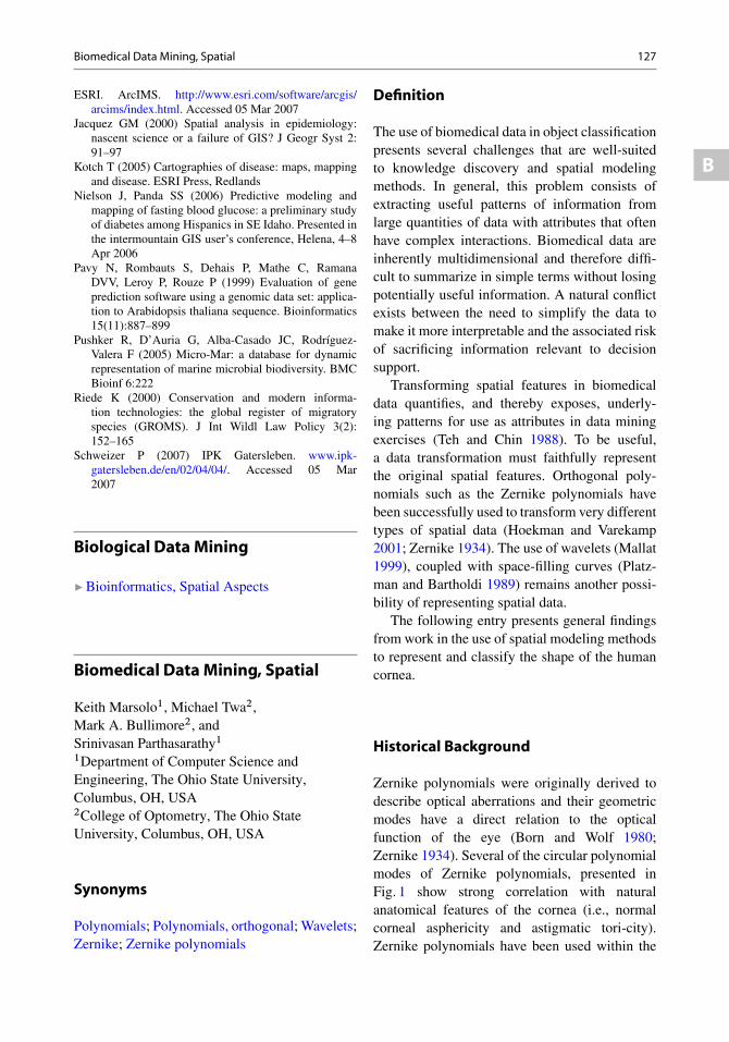
Biomedical Data Mining, Spatial 127

B

ESRI. ArcIMS. http://www.esri.com/software/arcgis/arcims/index.html. Accessed 05 Mar 2007

Jacquez GM (2000) Spatial analysis in epidemiology:nascent science or a failure of GIS? J Geogr Syst 2:91–97

Kotch T (2005) Cartographies of disease: maps, mappingand disease. ESRI Press, Redlands

Nielson J, Panda SS (2006) Predictive modeling andmapping of fasting blood glucose: a preliminary studyof diabetes among Hispanics in SE Idaho. Presented inthe intermountain GIS user’s conference, Helena, 4–8Apr 2006

Pavy N, Rombauts S, Dehais P, Mathe C, RamanaDVV, Leroy P, Rouze P (1999) Evaluation of geneprediction software using a genomic data set: applica-tion to Arabidopsis thaliana sequence. Bioinformatics15(11):887–899

Pushker R, D’Auria G, Alba-Casado JC, Rodríguez-Valera F (2005) Micro-Mar: a database for dynamicrepresentation of marine microbial biodiversity. BMCBioinf 6:222

Riede K (2000) Conservation and modern informa-tion technologies: the global register of migratoryspecies (GROMS). J Int Wildl Law Policy 3(2):152–165

Schweizer P (2007) IPK Gatersleben. www.ipk-gatersleben.de/en/02/04/04/. Accessed 05 Mar2007

Biological Data Mining

�Bioinformatics, Spatial Aspects

Biomedical Data Mining, Spatial

Keith Marsolo1, Michael Twa2,Mark A. Bullimore2, andSrinivasan Parthasarathy1

1Department of Computer Science andEngineering, The Ohio State University,Columbus, OH, USA2College of Optometry, The Ohio StateUniversity, Columbus, OH, USA

Synonyms

Polynomials; Polynomials, orthogonal; Wavelets;Zernike; Zernike polynomials

Definition

The use of biomedical data in object classificationpresents several challenges that are well-suitedto knowledge discovery and spatial modelingmethods. In general, this problem consists ofextracting useful patterns of information fromlarge quantities of data with attributes that oftenhave complex interactions. Biomedical data areinherently multidimensional and therefore diffi-cult to summarize in simple terms without losingpotentially useful information. A natural conflictexists between the need to simplify the data tomake it more interpretable and the associated riskof sacrificing information relevant to decisionsupport.

Transforming spatial features in biomedicaldata quantifies, and thereby exposes, underly-ing patterns for use as attributes in data miningexercises (Teh and Chin 1988). To be useful,a data transformation must faithfully representthe original spatial features. Orthogonal poly-nomials such as the Zernike polynomials havebeen successfully used to transform very differenttypes of spatial data (Hoekman and Varekamp2001; Zernike 1934). The use of wavelets (Mallat1999), coupled with space-filling curves (Platz-man and Bartholdi 1989) remains another possi-bility of representing spatial data.

The following entry presents general findingsfrom work in the use of spatial modeling methodsto represent and classify the shape of the humancornea.

Historical Background

Zernike polynomials were originally derived todescribe optical aberrations and their geometricmodes have a direct relation to the opticalfunction of the eye (Born and Wolf 1980;Zernike 1934). Several of the circular polynomialmodes of Zernike polynomials, presented inFig. 1 show strong correlation with naturalanatomical features of the cornea (i.e., normalcorneal asphericity and astigmatic tori-city).Zernike polynomials have been used within the

128 Biomedical Data Mining, Spatial

Biomedical Data Mining, Spatial, Fig. 1 Graphicalrepresentation of the modes that constitute a 4th orderZernike polynomial. Each mode is labeled using the singleindexing convention created by the Optical Society ofAmerica (Thibos et al. 1999)

medical community for a number of differentapplications, most recently for modeling theshape of the cornea (Schwiegerling et al. 1995).Studies have shown that these models caneffectively characterize aberrations that may existon the corneal surface (Iskander et al. 2001a, b).

The use of wavelets is natural in applicationsthat require a high degree of compression with-out a corresponding loss of detail, or where thedetection of subtle distortions and discontinuitiesis crucial (Mallat 1999). Wavelets have been usedin a number of applications, ranging from signalprocessing, to image compression, to numericalanalysis (Daubechies 1992). They play a largerole in the processing of biomedical instrumentdata obtained through techniques such as ultra-sound, magnetic resonance imaging (MRI) anddigital mammography (Laine 2000).

Scientific Fundamentals

Zernike PolynomialsZernike polynomials are a series of circular poly-nomials defined within the unit circle. They areorthogonal by the following condition:

Z 2�

0

Z 1

0

Zmn .�; /ZR

m0

n0 .�; /�d�d

D�

2.nC 1/ınn0ımm0 (1)

where ı is the Kronecker delta. Their computa-tion results in a series of linearly independent cir-cular geometric modes that are orthonormal withrespect to the inner product given above. Zernikepolynomials are composed of three elements:a normalization coefficient, a radial polynomialcomponent and a sinusoidal angular component(Thibos et al. 1999). The general form for Zernikepolynomials is given by:

Zmn .�; /

D

8<

:

p2.nC 1/ZRm

n .�/ cos.m/ for m > 0p2.nC 1/ZRm

n .�/ sin.jmj/ for m < 0p.nC 1/ZRm

n .�/ for m D 0

(2)

where n is the radial polynomial order and m

represents azimuthal frequency. The normaliza-tion coefficient is given by the square root termpreceding the radial and azimuthal components.The radial component of the Zernike polynomial,the second portion of the general formula, isdefined as:

ZRmn .�/

D

.n�jmj/=2X

sD0

.�1/s.n � s/Š

sŠ.nCjmj2

� s/Š.n�jmj2

� s/Š�n�2s:

(3)

Note that the value of n is a positive integer orzero. For a given n, m can only take the values�n, �n C 2, �n C 4, : : :, n. In other words,m � jnj D even and jnj < m. Thus, only certaincombinations of n and m will yield valid Zernikepolynomials. Any combination that is not validsimply results in a radial polynomial componentof zero.

Polynomials that result from fitting raw datawith these functions are a collection of approxi-mately orthogonal circular geometric modes. Thecoefficients of each mode are proportional to itscontribution to the overall topography of the orig-inal image data. As a result, one can effectivelyreduce the dimensionality of the data to a subsetof polynomial coefficients that represent spatial

Biomedical Data Mining, Spatial 129

B

features from the original data as the magnitudeof discrete orthogonal geometric modes.

WaveletsGiven a decomposition level S and a one-dimensional signal of length N , where N isdivisible by 2S , the discrete wavelet transformconsists of S stages. At each stage in thedecomposition, two sets of coefficients areproduced, the approximation and the detail.The approximation coefficients are generated byconvolving the input signal with a low-pass filterand down-sampling the results by a factor of two.The detail coefficients are similarly generated,convolving the input with a high-pass filter anddown-sampling by a factor of two. If the finalstage has not been reached, the approximationcoefficients are treated as the new input signal andthe process is repeated. In many cases, once thewavelet transformation is complete, the originalsignal will be represented using combinationsof approximation and detail coefficients. In theapplications presented here, however, only thefinal level of approximation coefficients are used.The rest are simply ignored.

To operate on a two-dimensional signal ofsize N � N (with N divisible by 2S ), the de-composition proceeds as follows: First, the rowsare convolved with a low-pass filter and down-sampled by a factor of two, resulting in matrixL (N=2 � N ). The process is repeated on theoriginal signal using a high-pass filter, whichleads to matrix H (N=2 � N ). The columns ofL are convolved two separate times, once with alow-pass filter and again with a high-pass filter.After passing through the filters, the signals aredown-sampled by a factor of two. This results ina matrix of approximation (LL) and horizontaldetail coefficients (LH ), respectively (both ofsize N=2 � N=2). These steps are executed oncemore, this time on the columns of H , resultingin a matrix of diagonal (HH ) and vertical (HL)detail coefficients (again of size N=2 � N=2).The whole procedure can then be repeated onthe approximation coefficients contained in ma-trix LL. As in the one-dimensional case, onlythe final level of approximation coefficients areconsidered.

Space-Filling CurvesThe two-dimensional wavelet decompositionwill, to some degree, capture the spatial localityof the original data. There may be instances,however, where the data does not lend itselfto the two-dimensional decomposition and theone-dimensional transformation is preferred.In order to retain some of the spatial locality,space-filling curves can be used to sample thedata (Platzman and Bartholdi 1989). There area number of different space-filling curves, butthis work utilizes the Hilbert curve. Hilbertcurves can be used to generate a one-dimensionalsignal that visits every point in two-dimensionalspace. Figure 2 shows the Hilbert curves of first,second and third order. These curves can beused to sample a matrix of size 4, 16, and 81,respectively. Higher-order curves can be used tosample larger input matrices, or the input datacan be scaled to fit accordingly.

Corneal TopographyClear vision depends on the optical quality of thecorneal surface, which is responsible for nearly75% of the total optical power of the eye (Kielyet al. 1982). Subtle distortions in the shape of thecornea can have a dramatic effect on vision. Theprocess of mapping the surface features on thecornea is known as corneal topography (Mandell1996).

The use of corneal topography has rapidly in-creased in recent years because of the popularityof refractive surgical procedures such as laserassisted in-situ keratomileusis (LASIK). Cornealtopography is used to screen patients for cornealdisease prior to this surgery and to monitor the ef-fects of treatment after. It is also used to diagnoseand manage certain diseases of the eye, includ-ing keratoconus, a progressive, non-inflammatorycorneal disease that can lead to corneal transplant.

The most common method of determiningcorneal shape is to record an image of a seriesof concentric rings reflected from the corneal sur-face. Any distortion in corneal shape will cause adistortion of the concentric rings. By comparingthe size and shape of the imaged rings with theirknown dimensions, it is possible to mathemati-cally derive the topography of the corneal surface.

130 Biomedical Data Mining, Spatial

00

0 1 2 3 4 5 6 7 80

1

2

3

4

5

6

7

8

1

2

1 2 00

1

2

3

4

1 2 3 4

a b

c

Biomedical Data Mining, Spatial, Fig. 2 Graphical representation of first (a), second (b), and third-order Hilbertcurves (c). Curves used to sample matrices of size 4, 16, and 81, respectively

Figure 3 shows an example of the outputproduced by a corneal topographer for a patientsuffering from Keratoconus, a patient with a nor-mal cornea, and an individual who has undergoneLASIK eye surgery. The methods presented hereare intended to differentiate between these pa-tient groups. These images represent illustrativeexamples of each class, i.e., they are designedto be easily distinguishable by simple visual in-spection. The top portion of the figure shows theimaged concentric rings. The bottom portion ofthe image shows a false color map representingthe surface curvature of the cornea. This colormap is intended to aid clinicians and is largelyinstrument-dependent.

Key Applications

This section covers techniques employed to rep-resent the topography data with the above mod-eling methods, to use those representations to

classify corneal shape, and finally, to present theresults of those decisions to allow clinicians tovisually inspect the classification criteria.

Data TransformationThe data from a corneal topographer are largelyinstrument-specific but typically consist of a 3Dpoint cloud of approximately 7000 spatial coordi-nates arrayed in a polar grid. The height of eachpoint ´ is specified by the relation ´ D f .�; /,where the height relative to the corneal apexis a function of radial distance from the origin(�) and the counter-clockwise angular deviationfrom the horizontal meridian ( ). The inner andouter borders of each concentric ring consist ofa discrete set of 256 data points taken at a knownangle , but a variable distance �, from the origin.

ZernikeThe method described here is based on tech-niques detailed by Schwiegerling et al. (1995)and Iskander et al. (2001a). In summary, the

Biomedical Data Mining, Spatial 131

B

Biomedical Data Mining, Spatial, Fig. 3Characteristic corneal shapes for three patient groups.The top image shows a picture of the cornea and reflectedconcentric rings. The bottom image shows the false

color topographical map representing corneal curvature,with an increased curvature given a color in the redspectrum, decreased curvature in blue. From left to right:Keratoconus, Normal and post-refractive surgery

data is modeled over a user-selected circularregion of variable-diameter, centered on the axisof measurement. The generation of the Zernikemodel surface proceeds in an iterative fashion,computing a point-by-point representation of theoriginal data at each radial and angular loca-tion up to a user-specified limit of polynomialcomplexity. The polynomial coefficients of thesurface that will later be used to represent theproportional magnitude of specific geometric fea-tures are computed by performing a least-squaresfit of the model to the original data, using stan-dard matrix inversion methods (Schwiegerlinget al. 1995).

2D WaveletsTo create a model using the 2D wavelet decom-position, the data must first be transformed from

polar to Cartesian coordinates. Once this step hasbeen completed, the matrix is normalized to apower of 2, typically 64� 64 or 128� 128. Afternormalization, the 2D wavelet decomposition isapplied, with the final level of approximationcoefficients serving as the feature vector.

1D WaveletsThis section details two methods for transformingthe topography data into a 1D signal. The firstmethod is to simply trace along each ring in acounter-clockwise fashion, adding each of the256 points to the end of the signal. Upon reachingthe end of a ring, one moves to the next larger ringand repeats the process. Next, a 1D decomposi-tion is applied and the final level approximationcoefficients are taken to serve as a feature vectorfor classification. The second method involves

132 Biomedical Data Mining, Spatial

transforming the data into a distance matrix aswith the 2D wavelet decomposition. Then, onecan sample the data using a space-filling curve,which will result in a 1D representation of the 2Dmatrix.

ClassificationGiven a dataset of normal, diseased, and post-operative LASIK corneas, the above represen-tations were tested using a number of differ-ent classification strategies, including decisiontrees, Naïve Bayes, and neural networks. Thedata was modeled with Zernike polynomials andseveral polynomials orders were tested, rang-ing from 4 to 10. The experiments showed thatthe low-order Zernike polynomials, coupled withdecision trees, provided the best classificationperformance, yielding an accuracy of roughly9% (Marsolo et al. 2006; Twa et al. 2003). The2D, 1D Hilbert and 1D ring-based wavelet rep-resentations were tested as well. For the 2Drepresentation, a normalized matrix of size 128�

128 and a 3rd level decomposition yielded thehighest accuracy. For the Hilbert-based approach,a normalized matrix of size 64 � 64 and a 6thlevel transformation. With the ring-based model,the 7th level decomposition yielded the highestaccuracy. The accuracy of the different wavelet-based models was roughly the same, hoveringaround 80%, approximately 10% lower than thebest Zernike-based approach.

VisualizationWhile accuracy is an important factor in choosinga classification strategy, another attribute thatshould not be ignored is the interpretability ofthe final results. Classifiers like decision trees areoften favored over “black-box” classifiers suchas neural networks because they provide moreunderstandable results. One can manually inspectthe tree produced by the classifier to examine thefeatures used in classification. In medical imageinterpretation, decision support for a domain ex-pert is preferable to an automated classificationmade by an expert system. While it is importantfor a system to provide a decision, it is oftenequally important for clinicians to know the basisfor an assignment.

Part of the rationale behind using Zernikepolynomials as a transformation method overother alternatives is that there is a direct corre-lation between the geometric modes of the poly-nomials and the surface features of the cornea.An added benefit is that the orthogonality of theseries allows each term to be considered inde-pendently. Since the polynomial coefficients usedas splitting attributes represent the proportionalcontributions of specific geometric modes, onecan create a surface representation that reflectsthe spatial features deemed “important” in classi-fication. These features discriminate between thepatient classes and give an indication as to thespecific reasons for a decision.

The section below discusses a method thathas been designed and developed to visualizedecision tree results and aid in clinical decisionsupport (Marsolo et al. 2005). The first step ofthe process is to partition the dataset based onthe path taken through the decision tree. Next asurface is created using the mean values of thepolynomial coefficients of all the patients fallinginto each partition. For each patient, an individualpolynomial surface is created from the patient’scoefficient values that correspond to the splittingattributes of the decision tree. This surface iscontrasted against a similar surface that containsthe mean partition values for the same splittingcoefficients, providing a measure to quantify how“close” a patient lies to the mean.

Figure 4 shows a partial decision tree for a4th Zernike model. The circles correspond tothe Zernike coefficients used as splitting criteria,while the squares represent the leaf nodes. Inthis tree, three example leaf nodes are shown,one for each of the patient classes considered inthis experiment (K – keratoconus, N – normal,L – post-operative LASIK). The black trianglesare simply meant to represent subtrees that wereomitted from the figure in order to improve read-ability. While each node of the tree representsone of the Zernike modes, the numbers on eachbranch represent the relation that must be true inorder to proceed down that path. (If no relationis provided, it is simply the negation of therelation(s) on the opposing branch(es)). An objectcan be traced through the tree until a leaf node is

Biomedical Data Mining, Spatial 133

B

Biomedical Data Mining,Spatial, Fig. 4 Partialdecision tree for a 4th orderZernike model

Z–13

Z 04

Z33

Z 24

Z 13

Z 22

Z 00

≤ 2.88

≤ –4.04

≤ –401.83L

K

≤ 1.42

≤ 9.34

≤ 0.07

≤ –0.31

N

> 1.00

reached and the object is then assigned the labelof that leaf. Thus, given the tree in Fig. 4, if anobject had a Z�1

3 coefficient with a value � 2.88,one would proceed down the left branch. If thevalue was> 2.88, the right branch would be takenand the object would be labeled as keratoconus.In this manner, there is a path from the root nodeto each leaf.

As a result, one can treat each possible paththrough a decision tree as a rule for classifyingan object. For a given dataset, a certain num-ber of patients will be classified by each rule.These patients will share similar surface features.Thus, one can compare a patient against themean attribute values of all the other patientswho were classified using the same rule. This

comparison will give clinicians some indicationof how “close” a patient is to the rule average. Tocompute these “rule mean” coefficients, denotedrule, the training data is partitioned and the aver-age of each coefficient is calculated using all therecords in that particular partition.

For a new patient, a Zernike transformationis computed and the record is classified usingthe decision tree to determine the rule for thatpatient. Once this step has been completed, thevisualization algorithm is applied to produce fiveseparate images (illustrated in Fig. 5). The firstpanel is a topographical surface representing theZernike model for the patient. It is constructedby plotting the 3-D transformation surface as a2-D topographical map, with elevation denoted

134 Biomedical Data Mining, Spatial

−0.5

−200

−400

−600

−800

−1−1

0 0.5 1

0

1a b c

−0.5

−200

−400

−600

−800

−1−1

0 0.5 1

0

1

−0.5

20

0

−20

20

10

0

−10

−1−1

0 0.5 1

0

1

−0.5−1−1

0 0.5 1

0

0

0.2

0.4

1 2 3 4 5 6 7 8 9 101112131415−2

0

2

1 2 3 4 5 6 7 8 9 101112131415−1.5

−1

−0.5

0

1 2 3 4 5 6 7 8 9 101112131415

1

−0.5

−200

−400

−600

0

−1−1

0 0.5 1

0

1

−0.5

−200

−400

−600

−1−1

0 0.5 1

0

1

−0.5

5

0

−10

−5

4

02

−6−4−2

−1−1

0 0.5 1

0

1

−0.5−1−1

0 0.5 1

0

1

−0.5

−200

−400

−600

−1−1

0 0.5 1

0

1

−0.5

−200

−400

−600

−1−1

0 0.5 1

0

1

−0.5

−370

−365

−360

−355

−400

−395

−390

−385

−1−1

0 0.5 1

0

1

−0.5−1−1

0 0.5 1

0

1

Biomedical Data Mining, Spatial, Fig. 5 Example sur-faces for each patient class. (a) represents a Keratoconiceye, (b) a Normal cornea, and a post-operative LASIKeye. The top panel contains the Zernike representationof the patient. The next panel illustrates the Zernike

representation using the rule values. The third and fourthpanels show the rule surfaces, using the patient and rulecoefficients, respectively. The bottom panel consists of abar chart showing the deviation between the patient’s rulesurface coefficients and the rule values

by color. The second section contains a topo-graphical surface created in a similar manner byusing the rule coefficients. These surfaces areintended to give an overall picture of how thepatient’s cornea compares to the average corneaof all similarly-classified patients.

The next two panels in Fig. 5 (rows 3 and 4)are intended to highlight the features used in clas-sification, i.e., the distinguishing surface details.These surfaces are denoted as rule surfaces. Theyare constructed from the value of the coefficientsthat were part of the classification rule (the restare zero). The first rule surface (third panel ofFig. 5) is created by using the relevant coeffi-cients, but instead of the patient-specific values,the values of the rule coefficients are used. Thissurface will represent the mean values of thedistinguishing features for that rule. The secondrule surface (row 4, Fig. 5) is created in the samefashion, but with the coefficient values from thepatient transformation, not the average values.

Finally, a measure is provided to illustratehow close a patient lies to those falling in the

same rule partition. For each of the distinguishingcoefficients, the relative error between the patientand the rule is computed. The absolute value ofthe difference between the coefficient value ofthe patient and the value of the rule is taken anddivided by the rule value. A bar chart of theseerror values is provided for each coefficient (theerror values of the the coefficients not used inclassification are set to zero). This plot is intendedto provide a clinician with an idea of the influenceof the specific geometric modes in classificationand the degree that the patient deviates from themean.

The surfaces in Fig. 5 correspond to the threeexample rules shown in the partial tree foundin Fig. 4. For each of the patient classes, themajority of the objects were classified by theexample rule. Since these are the most discrimi-nating rules for each class, one would expect thatthe rule surfaces would exhibit surface featurescommonly associated with corneas of that type.These results are in agreement with expectationsof domain experts.

B-tree, Versioned 135

B

Future Directions

The above methods are not limited just to model-ing the shape of the cornea. They could be appliedto almost any domain dealing with structure-based data.

Cross-References

� Space-Filling Curves

References

Born M, Wolf E (1980) Principles of optics: electromag-netic theory of propagation, interference and diffrac-tion of light, 6th edn. Pergamon Press, Oxford/NewYork

Daubechies I (1992) Ten lectures on wavelets. Society forIndustrial and Applied Mathematics, Philadelphia

Hoekman DH, Varekamp C (2001) Observation of trop-ical rain forest trees by airborne high-resolution in-terferometric radar. IEEE Trans Geosci Remote Sens39(3):584–594

Iskander DR, Collins MJ, Davis B (2001a) Optimal mod-eling of corneal surfaces with Zernike polynomials.IEEE Trans Biomed Eng 48(1):87–95

Iskander DR, Collins MJ, Davis B, Franklin R (2001b)Corneal surface characterization: how many Zerniketerms should be used? (ARVO) abstract. Invest Oph-thalmol Vis Sci 42(4):896

Kiely PM, Smith G, Carney LG (1982) The mean shapeof the human cornea. J Modern Opt 29(8):1027–1040

Laine AF (2000) Wavelets in temporal and spatial pro-cessing of biomedical images. Annu Rev Biomed Eng02:511–550

Mallat S (1999) A wavelet tour of signal processing, 2ndedn. Academic, New York

Mandell RB (1996) A guide to videokeratography. IntContact Lens Clin 23(6):205-28

Marsolo K, Parthasarathy S, Twa MD, Bullimore MA(2005) A model-based approach to visualizing classifi-cation decisions for patient diagnosis. In: Proceedingsof the conference on artificial intelligence in medicine(AIME), Aberdeen, 23–27 July 2005

Marsolo K, Twa M, Bullimore MA, Parthasarathy S(2006) Spatial modeling and classification of cornealshape. IEEE Trans Inf Technol Biomed

Platzman L, Bartholdi J (1989) Spacefilling curves and theplanar travelling salesman problem. J Assoc ComputMach 46:719–737

Schwiegerling J, Greinvenkamp JE, Miller JM (1995)Representation of videokeratoscopic height data withZernike polynomials. J Opt Soc Am A 12(10):2105–2113

Teh C-H, Chin RT (1988) On image analysis by themethods of moments. IEEE Trans Pattern Anal MachIntell 10(4):496–513

Thibos LN, Applegate RA, Schwiegerling JT, Webb R(1999) Standards for reporting the optical aberrationsof eyes. In: TOPS, Santa Fe. OSA

Twa MD, Parthasarathy S, Raasch TW, Bullimore MA(2003) Automated classification of keratoconus: a casestudy in analyzing clinical data. In: SIAM interna-tional conference on data mining, San Francisco, 1–3May 2003

Zernike F (1934) Beugungstheorie des Schneidenver-fahrens und seiner verbesserten Form, der Phasenkon-trastmethode. Physica 1:689–704

Bi-temporal

� Spatiotemporal Query Languages

Bitmap

�Raster Data

Bivariate Median

�Geometric Median

Black Hole Detection

�Ring-Shaped Hotspot Detection

BLUP

� Spatial Econometric Models, Prediction

Branch and Bound

� Skyline Queries

B-tree, Versioned

� Smallworld Software Suite

136 Bubble Estimation

Bubble Estimation

� Financial Asset Analysis with Mobile GIS

Bundle Adjustment

� Photogrammetric Methods

Business Application

�Decision-Making Effectiveness with GIS

Bx-Tree

� Indexing of Moving Objects, Bx-Tree