Ballot order effects in direct democracy elections

John G. Matsusaka1

Received: 19 March 2016 /Accepted: 30 May 2016 / Published online: 16 June 2016� Springer Science+Business Media New York 2016

Abstract Many political practitioners believe that voters are more likely to approve

propositions listed at the top than the bottom of the ballot, potentially distorting democratic

decision making, and this belief influences election laws across the United States. Numerous

studies have investigated ballot order effects in candidate elections, but there is little evi-

dence for direct democracy elections, and identification of causal effects is challenging.

This paper offers two strategies for identifying the effect of ballot order in proposition

elections, using data from California during 1958–2014 and Texas during 1986–2015. The

evidence suggests that propositions are not advantaged by being listed at the top compared

to the bottom of the ballot. Approval rates are lower with more propositions on the ballot.

Keywords Direct democracy � Initiative � Referendum � Ballot proposition � Ballot order �Causality

1 Introduction

In the summer of 2012, allies of California Governor Jerry Brown persuaded the legislature

to amend the state’s elections code so that the governor’s tax-raising initiative would be

listed first among 11 propositions on the ballot. Although the change was officially

motivated by a desire to ensure that voters were able to ‘‘carefully weigh the consequences

of important measures’’ on the ballot, it was widely believed that the real purpose was to

increase the initiative’s chance of passing.1 Opponents of the initiative argued that the

& John G. Matsusakamatsusak@usc.edu

1 Marshall School of Business, Gould School of Law, Department of Political Science, University ofSouthern California, Los Angeles, USA

1 The findings and declarations in the new law (AB 1499) stated: ‘‘bond measures and constitutionalamendments should have priority on the ballot because of the profound and lasting impact these measurescan have on our state…. In recognition of their significance, bond measures and constitutional amendments

123

Public Choice (2016) 167:257–276DOI 10.1007/s11127-016-0340-9

governor’s allies had cynically manipulated the elections code to secure the most favorable

position for the governor’s proposal. The implicit assumption in the debate was that ballot

position matters for direct democracy elections, and specifically, that the first position

confers an advantage.

The purpose of this paper is to assess the premise that ballot position influences the

outcomes of direct democracy elections. The idea that the top position is best is not new:

writing almost a half century ago, Mueller (1969, p. 1208) observed:

The state legislature devoutly believes in the existence of a body of citizens who start

out voting affirmatively on bond issues but turn to negativism as they move down the

ballot viewing with mounting horror the extent of the proposed expenditures. Part of

the reason for placing state bond issues at the top of the ballot is to catch the

affirmative votes of these citizens before they turn sour.

Theoretically, the top position may be advantageous if voters become fatigued moving

down the ballot, and if decision fatigue causes a status quo bias that leads to rejection of new

proposals.2 Empirically, there is a healthy literature on order effects in candidate elections,

but little evidence on order effects in proposition elections. Given the apparent existence of

order effects in candidate elections, the widespread belief of order effects among political

practitioners, and the role of this belief in framing election law, it seems worthwhile to

estimate the extent to which ballot structure actually matters for direct democracy elections.

Our current knowledge of order effects in direct democracy elections is limited by a

dearth of evidence that is convincingly causal in nature. The main contribution of this

paper is to offer evidence that addresses common challenges to causal inference. First,

since 1986 Texas has assigned ballot positions for propositions by lottery, producing

randomized experimental data. The mean observed approval rates can be compared across

ballot positions to provide direct estimates of ballot order effects. Second, in California, the

Field Poll routinely surveys likely voters about their voting intentions on select ballot

propositions in a way that is not closely linked to the order in which the propositions will

appear in the ballot. These survey responses capture voter preferences about a proposition

independent of the proposition’s position on the ballot. Ballot position effects can then be

inferred by comparing each proposition’s approval rate when ‘‘treated’’ with its actual

ballot position to its expressed pre-election Field Poll approval rate (the ‘‘control’’).

The main finding is a consistent absence of evidence that the top (or any) position on the

ballot is particularly favorable. Election data for the 240 Texas propositions during

1986–2015 show a correlation of -0.01 between ballot position and approval rates, and

parametric estimates controlling for other factors also fail to reveal a meaningful con-

nection. Similarly, an examination of the 242 California propositions during 1958–2014 for

which Field Poll data are available fails to reveal a robust effect of ballot position on

approval rates after controlling for pre-election opinion.

The evidence from Texas and California points in the same direction and is complementary

given the dissimilarity in the electoral contexts of the two states. Texas proposition elections

typically take place in odd-numbered years in which nomajor candidate races are on the ballot

and feature somewhat technical amendments to the constitution proposed by the legislature,

Footnote 1 continuedshould be placed at the top of the ballot to ensure that the voters can carefully weigh the consequences ofthese important measures.’’2 For discussion and variants on this idea, see Miller and Krosnick (1998), Bowler and Donovan (1998),Levav et al. (2010), and Augenblick and Nicholson (2016).

258 Public Choice (2016) 167:257–276

123

while California elections often feature controversial voter initiatives that attract significant

public attention and appear on the same ballot as high-profile candidate elections. One could

argue that ballot order effects aremore likely to occur in low turnout, low information elections

(Texas) or in high turnout, high information elections (California); the absence of an effect in

both cases using different methods suggests the finding may be fairly general.

I also explore the related issue of ballot length. Practitioners and scholars argue that the

information requirements associated with long ballots can overwhelm voters, causing the

status quo bias to kick in and leading to more ‘‘no’’ votes. It is not difficult to find examples

of elections that voters must have found challenging, such as the 1914 California general

election in which voters had to decide 48 ballot propositions. The danger of overloading

voters has led some states to establish limits on the number of propositions that can appear

on a ballot. For example, Arkansas and Illinois limit the number of legislative constitu-

tional amendments to three, and Mississippi has a cap of five initiatives per ballot. Previous

research suggests that voters are more likely to reject a proposition when it appears on a

ballot with many other propositions (Bowler and Donovan 1998) and, more generally, that

the size of the choice set affects decision making (Selb 2008; Iyengar and Kamenica 2010).

This study’s estimates on ballot length are less compelling in terms of causal inference than

the order estimates, but reveal a consistently lower approval rate for propositions on long

compared to short ballots.

The initial motivation for this paper was to evaluate the premise underlying a live policy

issue. However, the evidence also speaks to broader issues in public choice. In terms of

voter behavior, some evidence suggests that decision making is cognitively costly (e.g.,

Baumeister et al. 1998; Danziger et al. 2011); if voters deplete their mental resources when

faced with numerous decisions, their choices may not be rational. The evidence reported

here suggests that decision fatigue does not cause order effects in ballot proposition

elections, but it may matter when ballots become too long. At an even broader level, direct

democracy continues to play a leading role in public policy making in the United States.

Ballot propositions have been a central arena for contesting emerging social issues such as

same-sex marriage and marijuana legalization, and for making expensive fiscal decisions;

for example, voters have decided whether to authorize over $195 billion worth of bond

propositions since 2000.3 Direct democracy is motivated by the belief that laws passed by

the voters are more likely to reflect their preferences than laws passed by legislatures, so it

would be of concern if non-preference factors such as ballot design turned out to have a big

effect on outcomes. The evidence in this paper suggests that, on average, ballot position is

unlikely to have a large effect on election outcomes, somewhat allaying that concern.

2 Institutional context: California

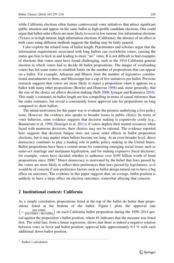
As a simple correlation, propositions listed at the top of the ballot do better than propo-

sitions listed at the bottom of the ballot. Figure 1 plots the approval rate

¼ yesvotesyesvotesþnovotes

� �on each California ballot proposition during the 1958–2014 per-

iod against the proposition’s ballot position, where #1 indicates that the measure was listed

first. The solid line, from a linear regression, shows that there is indeed a negative relation

between votes in favor and ballot position; approval falls approximately 0.5 % with each

additional down-ballot position.

3 Author’s calculation.

Public Choice (2016) 167:257–276 259

123

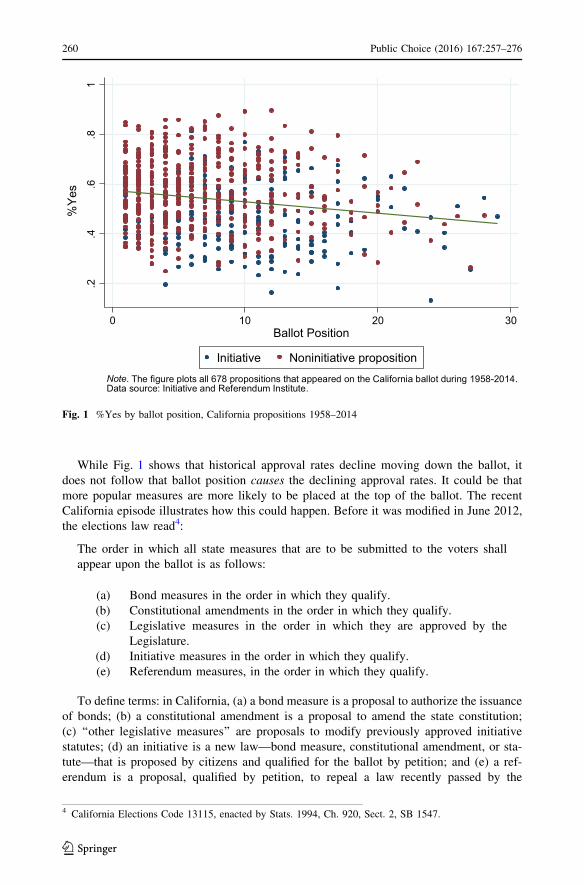
While Fig. 1 shows that historical approval rates decline moving down the ballot, it

does not follow that ballot position causes the declining approval rates. It could be that

more popular measures are more likely to be placed at the top of the ballot. The recent

California episode illustrates how this could happen. Before it was modified in June 2012,

the elections law read4:

The order in which all state measures that are to be submitted to the voters shall

appear upon the ballot is as follows:

(a) Bond measures in the order in which they qualify.

(b) Constitutional amendments in the order in which they qualify.

(c) Legislative measures in the order in which they are approved by the

Legislature.

(d) Initiative measures in the order in which they qualify.

(e) Referendum measures, in the order in which they qualify.

To define terms: in California, (a) a bond measure is a proposal to authorize the issuance

of bonds; (b) a constitutional amendment is a proposal to amend the state constitution;

(c) ‘‘other legislative measures’’ are proposals to modify previously approved initiative

statutes; (d) an initiative is a new law—bond measure, constitutional amendment, or sta-

tute—that is proposed by citizens and qualified for the ballot by petition; and (e) a ref-

erendum is a proposal, qualified by petition, to repeal a law recently passed by the

.2.4

.6.8

1

%Y

es

0 10 20 30Ballot Position

Initiative Noninitiative proposition

Note. The figure plots all 678 propositions that appeared on the California ballot during 1958-2014.Data source: Initiative and Referendum Institute.

Fig. 1 %Yes by ballot position, California propositions 1958–2014

4 California Elections Code 13115, enacted by Stats. 1994, Ch. 920, Sect. 2, SB 1547.

260 Public Choice (2016) 167:257–276

123

legislature.5 As can be seen, the original elections code placed legislative proposals (bond

issues, constitutional amendments, statutes) first, followed by citizen proposals (initiatives

and referendums). Within each category, propositions were ordered by the date at which

they qualified for the ballot.6 After June 2012, the elections code became7:

The order in which all state measures that are to be submitted to the voters shall

appear upon the ballot is as follows:

(a) Bond measures, including those proposed by initiative, in the order in

which they qualify.

(b) Constitutional amendments, including those proposed by initiative, in the

order in which they qualify.

(c) Other Legislative measures, other than those described in subdivision

(a) or (b), in the order in which they are approved by the Legislature.

(d) Initiative measures, other than those described in subdivision (a) or (b), in

the order in which they qualify.

(e) Referendum measures, in the order in which they qualify.

The new code blurs the distinction between legislative and citizen-initiated proposals.

Now bond measures are listed first, regardless of whether they originate from the legis-

lature or citizen petition, followed by constitutional amendments, regardless of whether

they originate from the legislature or petition. For non-bond statutory proposals, the

ordering stays the same: legislative proposals followed by citizen initiatives. Referendums

remain at the bottom of the ballot.8

The California elections code introduces several potential selection effects. First, prior

to 2012, it placed proposals from the legislature ahead of citizen proposals. Historically,

legislative measures have a much higher rate of passage than citizen measures; during the

period 1958–2014, 72 % of legislative proposals were approved compared to 37 % of

citizen-initiated proposals. This is probably because legislative proposals must garner

majority support in both chambers—supermajority support in the case of constitutional

amendments—so they are likely to have broader appeal than initiatives and referendums,

which require only signatures of a small percentage of the electorate.9 Second, bond

5 Ballot proposition terminology varies by state and country. In the California elections code, a ‘‘referen-dum’’ is a proposal to repeal a law passed by the legislature; in other jurisdictions it refers more generally toany popular vote on a law, whether proposed by citizens, the legislature, or other means. See Lupia andMatsusaka (2004) and Matsusaka (2005) for more details.6 The pre-2012 code is actually somewhat ambiguous. One could read the law to mean that a bond measureproposed by initiative is to be included in subdivision (a) and a constitutional amendment proposed byinitiative is to be included in subdivision (b). Under such an interpretation, subdivision (d) would apply onlyto non-bond, non-amendment initiatives. The text describes how the law was implemented in practice.7 An underline is new text; a strikethrough is deleted text. The code was modified by Stats. 2012, Ch. 30,Sect. 2.8 Governor Brown’s Proposition 30 was an initiative to amend the constitution. As an initiative, it wasoriginally included in subdivision (d), and because it qualified later in the election cycle than other ini-tiatives, it was slated to appear near the bottom of the ballot. By giving precedence to constitutionalamendments, whatever the source, the revised code moved the governor’s proposal to the top of the ballot;there were no bond propositions in that election and Proposition 30 was the only constitutional amendment.9 To reach the ballot, a bond proposal requires a majority vote in both the Assembly and Senate andsignature of the governor; a constitutional amendment requires a two-thirds vote in both chambers but doesnot require the governor’s signature; and a statute that amends an initiative requires a majority vote in bothchambers and signature of the governor. The initiative signature requirement, expressed as a percentage of

Public Choice (2016) 167:257–276 261

123

proposals must pass a different screening process than constitutional amendments (see

footnote 9), which could cause voters to view them differently, and voters may be more

hesitant to amend the constitution than to approve a bond measure. During the 1958–2014

period, voters approved 78 % of legislative bond measures, 69 % of legislative constitu-

tional amendments, and 76 % of legislative statutes. Third, measures that qualify at an

earlier date appear toward the top of the ballot. Proposals that are inherently more popular

may qualify earlier because it is easier to achieve a legislative consensus on them and

easier to collect the requisite signatures.

California’s practice of arranging the ballot by grouping issues and placing them in a

predetermined order is common. For example, most states give priority to issues according to

the times at which they qualify for the ballot. Arkansas, Arizona, Colorado, and North

Dakota place constitutional amendments before statutes. Maine places bond measures at the

bottom of the ballot. New Mexico and Rhode Island place constitutional amendments at the

top and bond measures at the bottom. Washington places advisory measures at the bottom of

the ballot. Because in most states we expect to see different approval rates for propositions at

the top compared to the bottom of the ballot for reasons having nothing to do with ballot

order, we cannot infer that that a correlation between approval and ballot position is causal.10

3 Theoretical considerations

The most common explanation for ballot order effects in candidate elections is drawn from

the psychology literature: satisficing and decision fatigue. The argument is that voters have

finite mental resources, and when working down a list, they stop once they find an

acceptable option rather than considering every possible option before making a choice.11

Being the first-listed candidate then would be an advantage. However, this argument

requires modification before it can be applied to proposition elections. To understand why,

note that in a candidate election, voters face a problem like the following:

Choose one:

h T. Butler

h A. Iommi

h J. Osborne

h W. Ward

Voters can select one and only one name from the list. If voters satisfice—stopping once

they find a ‘‘good enough’’ option—or become tired moving down a list, then appearing at

the top of the ballot in a candidate election would confer an advantage.

Footnote 9 continuedthe votes cast for governor in the previous election, is 8 % for constitutional amendments and 5 % forstatutes (since 1966); the requirement is 5 % for referendums.10 We can get a rough sense of the importance of the ballot ordering rules in California by estimating therelation between approval rates and ballot position with and without controls for type of proposition. Thecoefficient of -0.46 in Fig. 1 becomes -0.21 when dummy variables for initiatives, referendums, andlegislative measures are added to the regression, suggesting that about half of the negative relation is due toselection by type of measure. A negative relation (of smaller magnitude) appears if the sample is restrictedto only initiatives, only referendums, or only legislative measures.11 A related idea is the ‘‘primacy effect,’’ namely that people remember early items in a list better than lateritems.

262 Public Choice (2016) 167:257–276

123

The problem facing voters in a direct democracy election is different:

Proposition 1 Choose one: h Yes h No

Proposition 2 Choose one: h Yes h No

Proposition 3 Choose one: h Yes h No

Proposition 4 Choose one: h Yes h No

If voters become fatigued when moving down the list of propositions, we would expect

to see more abstention moving down the ballot, but it is less obvious why voters would be

more inclined to check the ‘‘No’’ box as they move down the ballot.

A rigorous and well-fleshed out theory of order effects in direct democracy elections has

yet to be provided, but the existing literature suggests the outlines of two theories based on

decision fatigue. The first (outline of a) theory relies on ‘‘confirmatory bias’’ (Miller and

Krosnick 1998): experimental evidence suggests that when faced with choices, people

begin by searching their memory for reasons that would lead them to select an option rather

than reasons not to select an option. As they become fatigued, they think less and less about

each option and become less likely to generate supportive thoughts. If we view voting

‘‘yes’’ on a proposition as a confirming or supporting action, this argument implies that as

voters become fatigued they will become less likely to vote in favor of a proposition. The

second theory relies on risk aversion: fatigue causes voting against a proposition because

weary voters become averse to the risk inherent in new proposals (Bowler and Donovan

1998). Research suggests that as people become fatigued, they are more likely to choose

simple or default options (see Levav et al. 2010 for discussion and evidence.) If voters

consider the proposed new law to be more risky than the status quo—or feel that sticking

with the status quo is the safe or default option—then fatigue would lead to a greater

proclivity to support the status quo, that is, to vote ‘‘no’’.

To summarize, the literature has offered theoretical conjectures about how decision

fatigue might interact with behavioral biases to create ballot order effects. This paper

evaluates these hypotheses by testing whether ballot order effects are present in direct

democracy elections. The null hypothesis is simply that citizens do not vote differently

based on ballot position.

4 Existing evidence

The literature on ballot position effects in candidate elections is extensive. Miller and

Krosnick (1998), in a well-known survey, observe that while much research concludes that

candidates benefit from being listed first, the estimated effects often are small and research

designs do not distinguish causation from correlation. The more recent literature that

employs stronger research designs generally finds that the first position is advantageous

(Meredith and Salant 2013), but some studies find small or nonexistent order effects

(Alvarez et al. 2006; Ho and Imai 2008).

The existing literature on order effects using data from direct democracy elections is

modest. Early statistical evidence was compiled and published by the California Secretary

of State (1981). That study, entirely descriptive, reports the mean percentage of votes in

favor by ballot position for all California propositions from 1884 to 1980.12 The data show

an irregular pattern, with approval rates not obviously dropping when moving down the

ballot.

12 The data are reported in an unnumbered table with the heading, ‘‘Success Rate of Each Ballot Position.’’

Public Choice (2016) 167:257–276 263

123

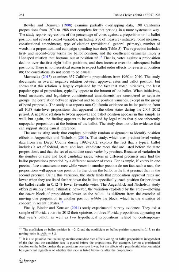
Bowler and Donovan (1998) examine partially overlapping data, 190 California

propositions from 1974 to 1988 (not complete for that period), in a more systematic way.

The study reports regressions of the percentage of votes against a proposition on its ballot

position and several control variables, including type of measure (initiative, bond measure,

constitutional amendment), type of election (presidential, general, primary), number of

words in a proposition, and campaign spending (see their Table 5). The regression includes

first- and second-order terms for ballot position, and the coefficient estimates imply a

U-shaped relation that bottoms out at position #8.13 That is, votes against a proposition

decline over the first eight ballot positions, and then increase over the subsequent ballot

positions. There is no theoretical reason to expect ballot order effects to reverse at position

#8; the correlations do not seem to be causal.

Matsusaka (2013) examines 637 California propositions from 1960 to 2010. The study

documents an overall negative relation between approval rates and ballot position, but

shows that this relation is largely explained by the fact that voter initiatives, the least

popular type of proposition, typically appear at the bottom of the ballot. When initiatives,

bond measures, and legislative constitutional amendments are considered as separate

groups, the correlation between approval and ballot position vanishes, except in the group

of bond proposals. The study also reports non-California evidence on ballot position from

all 1058 state-level propositions that appeared in the other states during the 2003–2012

period. A negative relation between approval and ballot position appears in this sample as

well, but again, the finding appears to be explained by legal rules that place inherently

unpopular propositions at the bottom of the ballot. The study does not offer evidence that

can support strong causal inference.

The one existing study that employs plausibly random assignment to identify position

effects is Augenblick and Nicholson (2016). That study, which uses precinct-level voting

data from San Diego County during 1992–2002, exploits the fact that a typical ballot

includes a set of federal, state, and local candidate races that are listed before the state

propositions, and that the set of candidate races varies by precinct. Because of variation in

the number of state and local candidate races, voters in different precincts may find the

ballot propositions preceded by a different number of races. For example, if voters in one

precinct face a state senate race while voters in another precinct do not face such a race, the

propositions will appear one position farther down the ballot in the first precinct than in the

second precinct. Using this variation, the study finds that proposition approval rates are

lower when they are listed farther down the ballot; specifically, each position farther down

the ballot results in 0.12 % fewer favorable votes. The Augenblick and Nicholson study

offers plausibly causal estimates; however, the variation exploited by the study—moving

the entire block of propositions lower on the ballot—is different from the exercise of

moving one proposition to another position within the block, which is the situation of

concern in recent debates.14

Finally, Binder and Kousser (2014) study experimental survey evidence. They ask a

sample of Florida voters in 2012 their opinions on three Florida propositions appearing on

that year’s ballot, as well as two hypothetical propositions related to contemporary

13 The coefficient on ballot-position is -2.12 and the coefficient on ballot-position-squared is 0.13, so the

turning point is 2:122�0:13 ¼ 8:2.

14 It is also possible that including another candidate race affects voting on ballot propositions independentof the fact that the candidate race is placed before the propositions. For example, having a presidentialelection on the ballot pushes the propositions one spot lower, but the effects of a presidential election mightbe significant regardless of whether that race is listed before or after the propositions.

264 Public Choice (2016) 167:257–276

123

California propositions, varying the order in which questions are asked. The findings are

mixed; some propositions do better when asked about first, while others do better when

asked about last.

To summarize, despite the contentiousness over proposition ordering in direct democ-

racy elections, the scholarly literature on order effects is limited and inconclusive. The

remainder if this paper offers two different types of new evidence, the first from Texas,

which offers randomized data, and the second from California.

5 Evidence from Texas

5.1 Methods and data

The Texas data are analyzed with a model of the following form:

VELECTit ¼ V�

it þ aþ b � POSit þ c � LENGTHit þ eit; ð1Þ

where VELECTit is the percentage of votes cast in favor of proposition i in election t, V�

it is the

(unobserved) ‘‘true’’ preferences of voters in the hypothetical situation where voting is

uninfluenced by ballot position, POSit is the measure’s ballot position (#1 is the top of the

ballot, #2 is the second proposition, and so on), LENGTHit is the number of propositions on

the ballot, eit is an error term, and a, b, c are parameters to be estimated. If voters are less

inclined to approve as they move down the ballot, then b\0.

The estimation challenge is that V�i is not observable; if we omit V�

i and simply regress

votes on ballot position, we have a textbook omitted variables problem, and the estimates

of b will be biased if V�i is correlated with ballot position. One way to avoid this problem is

to randomize ballot position, as Texas has done since 1986.15 With positions assigned

randomly, there is no reason to expect the underlying popularity of a measure to be related

to its ballot position; therefore, omitting V�i from estimates of (1) should not introduce a

bias in the estimate of b. The strategy then is simply to investigate whether propositions at

the top of the ballot attract more favorable votes than those at the bottom of the ballot.

The data are drawn from official election results published by the Texas Secretary of

State. Summary information on the 240 Texas propositions that appeared during 1986–

2015 are reported in Panel A of Table 1. Texas does not allow initiatives or referendums,

and the legislature does not place statutes on the ballot; therefore, all propositions are

constitutional amendments proposed by the legislature. The main variable of interest,

VELECTit , is operationalized as the approval rate, or ‘‘%Yes’’, defined to be

%Yes ¼ 100� yes votesyes votes + no votes. Abstentions are ignored.16

15 Texas Election Code, Title 16, Chapter 274, Subchapter A, Sect. 274.002. The relevant text is: ‘‘If morethan one proposed constitutional amendment is to be submitted in an election, the order of the propositionssubmitting the amendments shall be determined by a drawing… ‘‘To the best of my knowledge, no study hasexploited yet the randomization of proposition order in Texas; see Grant (2016) for a study of order effectsin candidate elections in Texas that exploits the randomization of candidate positions, finding large effects.16 For reasons of space, this study does not consider the interesting phenomenon of abstention or ‘‘roll off.’’Ignoring this consideration should not affect the estimates of how ballot structure influences approval ratessince approval rates are net of participation issues.

Public Choice (2016) 167:257–276 265

123

5.2 Findings

Figure 2 plots the approval rate for Texas propositions against their ballot positions. The

solid line is a regression of approval on position. The regression line is almost completely

flat, indicating essentially no connection, on average, between ballot position and approval

rates. This is initial evidence against the hypothesis that position has an important effect on

approval rates.

Table 2 extends the investigation by reporting regressions of the approval rate on ballot

position. Each column in the table reports results from a regression. Column (1) reports a

regression representing the solid line in Fig. 2. Taken at face value, the coefficient of

-0.03 on ballot position indicates that each position further down the ballot is associated

with 0.03 % fewer votes in favor, a small number that cannot be distinguished from zero

statistically.

The remaining regressions of Table 2 include a variable equal to the number of

propositions on the ballot. Column (2) shows a positive relation between ballot position

and votes in favor, again statistically insignificant, and a negative relation between ballot

length and votes in favor. The coefficient -0.40 on ballot length implies that each addi-

tional proposition on the ballot is associated with 0.40 % fewer votes in favor. This

coefficient is different from zero at the 1 % level of statistical significance. The regression

in column (3) is the same as the regression in column (2) except that extreme values of the

Table 1 Summary statistics for Texas and California propositions

Variable Mean SD Min Max

Panel A. Texas propositions, 1986–2015

%Yes (election) 63.4 12.6 30.2 93.8

Position 8.5 5.9 1 27

Number of propositions on ballot 16.0 6.4 1 27

Variable Field Poll sample(N = 242)

All props (N = 678)

Mean SD Min Max Mean

Panel B. California propositions, 1958–2014

%Yes (election) 48.6 12.5 13.3 74.2 53.8

%Yes (Field Poll) 54.5 13.5 19.1 89.0 NA

%Yes (election)–%Yes (Field Poll) -6.0 8.1 -30.4 14.3 NA

Position 8.5 5.8 1 29 7.8

Number of propositions on ballot 14.1 7.1 1 29 14.6

Type = legislative bond measure 0.23 0.42 0 1 0.22

Type = initiative 0.70 0.46 0 1 0.34

Dummy = 1 presidential election year 0.51 0.50 0 1 0.47

This table reports summary statistics for the Texas (Panel A) and California (Panel B) data. Texas datainclude 240 propositions. All Texas propositions were constitutional amendments placed on the ballot by thelegislature. California data include 678 propositions, 242 of which were surveyed in the Field Poll. Panel Breports the mean approval rate for Field Poll propositions and for all propositions (those included andexcluded from Field Poll) during the period

266 Public Choice (2016) 167:257–276

123

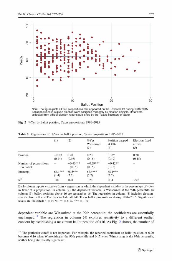
dependent variable are Winsorized at the 99th percentile; the coefficients are essentially

unchanged.17 The regression in column (4) explores sensitivity to a different outlier

concern by establishing a maximum ballot position of #16. As Fig. 2 shows, the number of

2040

6080

100

Yes

%

0 10 20 30Ballot Position

Note. The figure plots all 240 propositions that appeared on the Texas ballot during 1986-2015.Ballot positions in a given election were assigned randomly by election officials. Data werecollected from official election reports published by the Texas Secretary of State.

Fig. 2 %Yes by ballot position, Texas propositions 1986–2015

Table 2 Regressions of %Yes on ballot position, Texas propositions 1986–2015

(1) (2) %YesWinsorized(3)

Position cappedat #16(4)

Election fixedeffects(5)

Position -0.03(0.14)

0.20(0.16)

0.20(0.16)

0.32*(0.19)

0.20(0.15)

Number of propositionson ballot

– -0.40***(0.15)

-0.39***(0.15)

-0.42**(0.15)

–

Intercept 64.1***(1.4)

68.5***(2.2)

68.4***(2.2)

68.1***(2.2)

–

R2 .001 .028 .028 .034 .272

Each column reports estimates from a regression in which the dependent variable is the percentage of votesin favor of a proposition. In column (2), the dependent variable is Winsorized at the 99th percentile. Incolumn (3), ballot positions above 16 are restated as 16. The regression in column (4) includes election-specific fixed effects. The data include all 240 Texas ballot propositions during 1986–2015. Significancelevels are indicated: * = 10 %, ** = 5 %, *** = 1 %

17 The particular cutoff is not important. For example, the reported coefficient on ballot position of 0.20becomes 0.16 when Winsorizing at the 90th percentile and 0.17 when Winsorizing at the 95th percentile,neither being statistically significant.

Public Choice (2016) 167:257–276 267

123

propositions with positions greater than #15 is rare, so the column (4) specification reduces

the chance that the few extreme positions are driving the result. The coefficient on ballot

position remains positive and is now statistically different from zero at the 10 % level,

suggesting an advantage to appearing near the bottom of the ballot. The coefficient on

ballot length is essentially the same.18

One concern with the regressions in columns (2)–(4) is that ballot position and ballot

length are to some extent positively correlated for mechanical reasons. This could cause

the ballot position coefficient to absorb ballot length effects, and vice versa. The regression

in column (5) avoids this problem by including election-specific fixed effects; in this case

the ballot position coefficient is estimated based on within-ballot variation, and thus is free

from ballot length effects. As can be seen, the coefficient on ballot position remains

positive, with the magnitude similar to other specifications, and without statistical

significance.19

Following Augenblick and Nicholson (2016), we can estimate how many election

outcomes would have come out differently if every proposition had appeared in the first

position, that is, if no proposition suffered the consequences of being listed other than first.

To do this, we calculate the implied change in each proposition’s approval rate based on

the coefficient on ballot position and the proposition’s actual ballot position, and compare

this to its margin of victory or defeat. Using the estimate in column (1), where appearing

down the ballot is disadvantageous, only one of one of the 240 propositions would have

gone from fail to approve if listed at the top of the ballot. Using the estimate in column (5)

where appearing down the ballot is advantageous, no proposition would have gone from

approval to failure if listed at the top instead of its actual position. In contrast to

Augenblick and Nicholson (2016), which concludes that 6 % of elections would have been

different without ballot order effects, I find that ballot order was a determining factor in

virtually no election outcomes in Texas.20

Statistically insignificant coefficients on ballot position do not rule out order effects;

they only imply that we are unable to distinguish any potential effects from noise. To get a

sense of what size effects are plausible with these data, we can add or subtract two standard

errors to find the maximum and minimum coefficients that can be rejected at the 95 %

confidence level. Those bounds range from 0.09 to 0.49, meaning that any effects outside

those bands can be rejected statistically. Thus, even if being listed down the ballot costs

votes, it is likely that the cost is extremely small. In contrast, there appears to be a reliably

negative relation between approval rates and ballot length.

18 The positive coefficient is robust to alternative caps. For example, setting the maximum position at #10yields a coefficient of 0.51 on ballot position; capping at position #20 yields a coefficient of 0.24.19 The regressions assume a linear relation between approval rate and ballot position, but Eq. (1) allows forany sort of nonlinearity. I estimated a variety of models with alternative specifications—for example,including second-order terms and allowing for differential effects in the first position—and did not findrobust evidence of order effects with these more complicated specifications either.20 The reason for the discrepancy is unclear. Perhaps elections are more competitive in San Diego Countythan Texas, so small effects are more likely to swing an election. Another possibility is that the Augenblickand Nicholson (2016) estimates overstate the consequences by not considering the effect of switchingposition within the block of propositions, but of jumping a proposition to the top of the entire ballot, aheadof all candidate elections; no propositions appear in such a position in their data—projecting outside thesupport of their data may produce unreliable predictions.

268 Public Choice (2016) 167:257–276

123

6 California

6.1 Methods and data

Recall that the core problem in estimating (1) is that V�i typically is not observable. The

research strategy for the California data is to use pre-election opinion surveys to proxy for

V�it . If survey responses do not depend on ballot position (more on this below), then we can

assume that they are generated according to:

VSURVEYit ¼ V�

it þ kþ lXit þ uit; ð2Þ

where VSURVEYit is the percentage of respondents who express support for proposition i, Xit

includes factors that cause survey responses to differ from underlying preferences, k is a

fixed survey ‘‘bias’’ (for example, pre-election polls in California systematically overstate

support for propositions), and uit is an error term that is independent across propositions.

The difference between election returns and pre-election survey results (called the

‘‘gap’’) is denoted by D, which from (1) and (2) can be expressed as:

Dit ¼ VELECTit � VSURVEY

it ¼ a� kþ b � POSit þ cZit � lXit þ eit � uit: ð3Þ

Then we can regress D on ballot position to recover the position effects without needing

to know the electorate’s underlying preferences. The estimate of b will be unbiased even if

ballot position is determined by underlying preferences rather than being assigned ran-

domly. Another advantage of specification (3) is that it is not necessary to control for

determinants of the vote choice itself because they are subsumed in the Vit variable.

A less formal way to think about this empirical strategy is that it uses pre-election

survey information to reveal the ‘‘untreated’’ preferences on a proposition. This expressed

preference is compared to the actual election outcome that has been ‘‘treated’’ with the

position effect, and the difference is used to infer the treatment effect. A potential limi-

tation of using pre-election survey data as a control is the possibility that preferences

change between the time of the poll and the election, or that voters express preferences in

an opinion survey that differ from their true beliefs. However, to the extent that there are

systematic biases in the survey, they will be absorbed into the intercept term, and will not

confound inferences as long as they are not correlated with ballot position.

The core data are election returns from Statement of Vote, published by the California

Secretary of State, and pre-election survey data from the Field Poll, available at www.field.

com, and the Field Research Data at UC Berkeley at ucdata.berkeley.edu/data.php. If the

Field Poll conducted multiple surveys on a proposition, I use data from the final survey,

that is, the one closest to the election. The Field Poll runs from 1958 to 2014. Of the 678

propositions that went before the voters during that time, Field Poll data are available for

242 of them.

The variables VELECTit and VSURVEY

it are operationalized as ‘‘yes’’ votes as a percentage of

all votes. Abstainers or, in the case of a survey, individuals who decline to state or fail to

give an opinion in favor or against are ignored. The gap between the election outcome and

pre-election survey is defined as D ¼ %YesELECT �%YesField Poll.

Summary statistics for California propositions are reported in Panel B of Table 1. The

propositions in the sample are not representative of all propositions that appeared on the

ballot because the Field Poll focuses on high-profile or controversial propositions. Field

Poll propositions are less popular than other propositions, with a mean vote in favor of

48.6 % compared to 53.8 % for all propositions that reach the ballot. Field Poll

Public Choice (2016) 167:257–276 269

123

propositions are much more likely than the full set of propositions to be initiatives (70 %

vs. 34 %), and much less likely to be legislative proposals (27 % vs. 65 %).

Table 1 shows that the final Field Poll before an election exceeds the percentage of

favorable votes in the election by 6.0 %, on average. This indicates a systematic ‘‘bias’’ in

the Field Poll, or alternatively, a predictable tendency for support to deteriorate leading up

to an election. Many election observers have noted that support for propositions tends to

deteriorate over time; Table 1 provides a large-sample quantification of the effect. The

deterioration may occur because proponents are usually the first to mobilize—they have to

secure legislative approval or collect signatures—and their arguments are the first to reach

the voters. As the campaign progresses, opponents make their case and some voters change

their mind. This deterioration in support between the last survey and the election is not a

problem for the identification exercise as long as deterioration is uncorrelated with ballot

position.21

The empirical analysis assumes that Field Poll responses are not influenced by ballot

position. This assumption would be questionable if the Field Poll asked voters about all

propositions on the ballot in the same order that they appeared on the ballot. That is not the

case. As noted above, the Field Poll conducted surveys for only 36 % of propositions on

the ballot. Furthermore, only 14 % of the surveys included all of the questions, and in 37 %

of the surveys the questions were not asked in the order in which they appeared on the

ballot. For example, the 2002 general election featured seven ballot measures; the Field

Poll asked about four of them in this order: Proposition 47-50-49-52.22 The order on the

ballot was 46-47-48-49-50-51-52. The survey contains omissions as well as re-orderings

and does not simply reproduce the actual ballot positions.23

Finally, it is worth emphasizing that the Field Poll does not select issues at random.

Rather, it chooses issues that are likely to be of interest to the public or policymakers. This

should not create a bias in the coefficients of interest, but it does affect external validity.

The California results should be seen as applying to relatively high-profile ballot issues.

The Texas data in some sense fill in the picture by providing evidence on lower profile

issues.

6.2 Findings

Figure 3 provides a characterization of the California data by plotting the mean gap (D) byposition, with 95 % confidence intervals indicated. Positions greater than #15 are collapsed

into a single group because of the paucity of observations. The means do not show a

consistent downward (or upward) pattern.

Table 3 reports statistical evidence from the California data: each column reports a

regression of the gap, D, on ballot position, following Eq. (3). The coefficient on ballot

position in column (1) is -0.07 (meaning that each position down the ballot reduces

approval by 0.07 %), quite small and far from statistical significance. Using the two-

standard-error rule of thumb, we can think of the potential effects as ranging from -0.31 to

0.17 %, which allows the possibility of nontrivial negative effect at the boundary. A

21 While plausible, the absence of such a correlation is not self-evident. For example, one might supposethat propositions near the top of the ballot were organized earlier than propositions at the bottom of theballot, and better organized propositions suffer less deterioration in support.22 The Field (California) Poll: Codebook 02-05, questions Q19 to Q26.23 In 1994, the Field Poll conducted surveys on four ballot propositions in a randomized order. Those resultsare summarized in the Appendix.

270 Public Choice (2016) 167:257–276

123

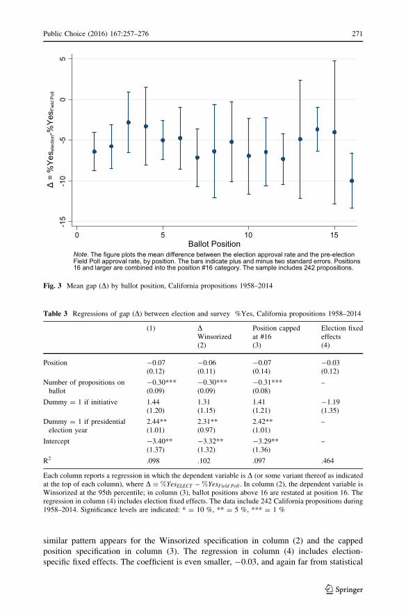
similar pattern appears for the Winsorized specification in column (2) and the capped

position specification in column (3). The regression in column (4) includes election-

specific fixed effects. The coefficient is even smaller, -0.03, and again far from statistical

-15

-10

-50

5Δ

= %

Yes

elec

tion-%

Yes

Fiel

d P

oll

0 5 10 15Ballot Position

Note. The figure plots the mean difference between the election approval rate and the pre-electionField Poll approval rate, by position. The bars indicate plus and minus two standard errors. Positions16 and larger are combined into the position #16 category. The sample includes 242 propositions.

Fig. 3 Mean gap (D) by ballot position, California propositions 1958–2014

Table 3 Regressions of gap (D) between election and survey %Yes, California propositions 1958–2014

(1) DWinsorized(2)

Position cappedat #16(3)

Election fixedeffects(4)

Position -0.07(0.12)

-0.06(0.11)

-0.07(0.14)

-0.03(0.12)

Number of propositions onballot

-0.30***(0.09)

-0.30***(0.09)

-0.31***(0.08)

–

Dummy = 1 if initiative 1.44(1.20)

1.31(1.15)

1.41(1.21)

-1.19(1.35)

Dummy = 1 if presidentialelection year

2.44**(1.01)

2.31**(0.97)

2.42**(1.01)

–

Intercept -3.40**(1.37)

-3.32**(1.32)

-3.29**(1.36)

–

R2 .098 .102 .097 .464

Each column reports a regression in which the dependent variable is D (or some variant thereof as indicatedat the top of each column), where D � %YesELECT �%YesField Poll. In column (2), the dependent variable isWinsorized at the 95th percentile; in column (3), ballot positions above 16 are restated at position 16. Theregression in column (4) includes election fixed effects. The data include 242 California propositions during1958–2014. Significance levels are indicated: * = 10 %, ** = 5 %, *** = 1 %

Public Choice (2016) 167:257–276 271

123

significance. The California data, like the Texas data, offer little reason to believe that

propositions benefit from being listed earlier on the ballot.

The California data also produce the pattern in the Texas data that propositions on

longer ballots receive fewer votes in favor, independent of the proposition’s own ballot

position. In column (1) of Table 3, each additional proposition on the ballot reduces the

approval rate by 0.30 % on average, a relation that is statistically significant at the 1 %

level, and similar in magnitude to what appears in the Texas sample. The coefficient on

ballot length is negative and statistically different from zero in regressions (2) and (3) as

well.

Another control variable is a dummy equal to one if the proposition was an initiative, as

opposed to a proposal from the legislature or a referendum. Initiatives might be expected to

attract more attention before the election, and therefore show less of a gap between election

approval and pre-election approval. This turns out not to be the case: the coefficient on the

initiative dummy suggests a larger gap for initiatives, although the coefficient is not

distinguishable from zero at conventional levels of significance in any of the regressions.

The final control variable is also related to information conditions, a dummy equal to one

for presidential election years. One could argue that voters pay more attention to politics in

presidential election years, and thus are more informed, or conversely, that a presidential

election draws voters to the polls who are uninformed about ballot propositions. The data

show a significantly wider gap in presidential election years, indicating that support does

not deteriorate as much in presidential election years.

I also estimated but do not report regressions under a variety of alternative specifications

in order to assess robustness of the findings. The alternatives included: allowing a separate

effect for the first position and for the last position; including higher order terms for ballot

position; including time dummies; including dummies for general as opposed to primary

elections; including dummies for bond propositions and for referendums; including con-

trols for the fraction of undecided voters; and alternative Winsorization cutoffs. For all of

these alternatives, it continued to be the case that no reliable relation could be found

between approval rates and ballot position.

7 Discussion and conclusion

State and local governments in the United States, and increasingly abroad, rely on ballot

propositions to resolve important public policy issues. More than 1800 state-level propo-

sitions have come before American voters in the twenty first century alone, addressing

high-profile and high-impact issues such as same-sex marriage, marijuana legalization,

taxes, and spending. The number of issues appearing in counties, cities, and towns is at

least an order of magnitude larger, and equally diverse. With citizen lawmaking playing a

central role in American democracy, it is important to identify mechanisms that might lead

to distortions in direct democracy decisions. One potential distortion—the order in which

issues are presented to voters—has long concerned practicing politicians, many of whom

believe that being listed at the top of the ballot is advantageous, and this belief has

influenced the design of state election laws. Yet research on the effect of ballot structure in

proposition elections remains scarce, and seldom allows causal inference.

This paper proposes and implements two different empirical strategies, both of which

are designed to distinguish causality from correlation. One strategy is to examine Texas

propositions since 1986, when the state began to place propositions on the ballot in a

272 Public Choice (2016) 167:257–276

123

random order. The other strategy is to use pre-election survey data from California, which

has a long history of polling on ballot measures, to control for public opinion independent

of ballot position. Both approaches fail to turn up robust evidence in support of the idea

that propositions attract more favorable votes when listed at the top of the ballot (or any

other position) than when listed elsewhere on the ballot. Because the evidence comes from

two rather different states and two different information environments—low-profile

measures in Texas in off-year elections versus high-profile issues in California—yet tells

the same story, the findings may have some generality. While it is difficult to prove a

negative, and variance around the estimates leaves some room for the possibility of modest

order effects, the evidence at hands points to the conclusion that ballot order effects are at

best rather small.

At first glance, these findings appear at odds with those of Augenblick and Nicholson

(2016). However, Augenblick and Nicholson do not actually study ballot order effects, as

conventionally defined; rather they investigate the effect of shifting the block of propo-

sitions as a group above or below the candidate elections on the same ballot. For example,

if a ballot begins with 10 candidate races in positions #1 to #10 and ends with 10

propositions in positions #11 to #20, Augenblick and Nicholson examine what would

happen if the propositions were moved to positions #1 to #10 but otherwise kept in the

same order. My study examines whether it matters to present propositions in a different

order, for example, for a particular proposition to be listed #11 versus #20.

In contrast to weak evidence for order effects, I find a robust negative relation between

approval rates and ballot length. Each additional proposition on the ballot is associated

with about 0.3 % lower approval for all propositions on that ballot. These estimates are

similar across various specifications, and hold for both California and Texas. On its own,

we might be tempted to attribute this finding to decision fatigue, but that seems paradoxical

given the absence of evidence for order effects. One way to square the two findings would

be if voters do not complete the ballot sequentially: they might come to the polling place

with a list of propositions they find important, and focus first on voting for those key

propositions and then disapprove the rest. If decision fatigue limits their set of key

propositions, then we could observe no order effects but lower approval on long ballots. An

explanation with some anecdotal appeal, unrelated to decision fatigue, is that voters dislike

long ballots in principle; if asked to resolve too many questions they sour on the entire

enterprise and are more likely to vote no on any given issue. This would cause an erosion

of support for every proposition on a long ballot, independent of position. A third possi-

bility is that the finding is spurious. The study is designed to provide causal estimates of the

order effect, but ballot length is not randomly assigned in the study. It could be that on

short ballots only the strongest propositions qualified, while on long ballots a number of

marginal propositions made the cut. Without a research design that allows stronger causal

inference, it is not possible to settle on an explanation, and the ballot length coefficient

ought to be interpreted with some care.

The policy implications of these findings are nuanced. In terms of providing a level

playing field, it appears that one should not be overly concerned with order manipulation

because the top of the ballot is not demonstrably better than the bottom. Even so, there is

no obvious downside to randomizing ballot position, so it would seem to be a useful

precaution. The evidence of lower approval rates on long ballots, if interpreted as a causal

effect, calls for some attention concerning ballot length. However, with no evidence as to

whether approval rates in general are too high or too low, it is difficult to conclude whether

the erosion of support on long ballots is a good or bad thing. Moreover, an attempt to

shorten ballots would mean that fewer issues reach the voters. Any benefits from higher

Public Choice (2016) 167:257–276 273

123

approval rates on short ballots would have to be balanced against the downside of cur-

tailing the number of public issues on which voters are allowed to decide.

Finally, the motivating example for this paper was California’s Proposition 30 that

catalyzed a revision of the California elections code. As discussed above, the revision was

widely seen as intended to help Proposition 30 pass. This study’s findings suggest that

simply moving the proposition to the top of the ballot was unlikely to have mattered.

However, there was another feature of that ballot that could change the story: a competing

initiative on the same ballot proposed a tax increase that was similar to the increase in

Proposition 30. Rather than decision fatigue, it could be that voters have a target budget in

mind and will only tax themselves (or approve spending) until that target budget is

depleted. If voters behave in that way, being listed first would be advantageous in order to

capture affirmative votes before voters exhaust their target budgets. This line of thinking

suggests that ballot order might matter in the context of competing proposals. As an

exploratory exercise, I returned to the California data and restricted the sample to bond

propositions (N = 55). I then created a variable equal to the number of bond propositions

that preceded each of the bond propositions on the ballot (i.e., the first bond proposition on

a ballot was preceded by zero bond propositions, the second was preceded by one bond

proposition, and so on). I then estimated a gap regression (3) that included the number of

preceding bond propositions as an explanatory variable. The coefficient on the new vari-

able was positive and statistically significant at the 10 % level, indicating that bond

propositions received more votes when they were preceded by other bond propositions,

contrary to what would be expected if voters have target budgets. Clearly, more rigorous

testing of this conjecture is needed.

Acknowledgments For helpful comments and suggestions, I thank Odilon Camara, Dan Klerman, andparticipants at the Initiatives and Referendums Conference at USC in November 2012 and the CLASSworkshop at USC. I thank USC for financial support.

Appendix

The Field Poll conducted a randomized controlled experiment in its survey for the June 7,

1994 primary election. I report this experiment here to bring it to the attention of

researchers in the area. The Field Poll exercise is similar to the experiment reported in

Binder and Kousser (2014). Four bond propositions were on the ballot, Propositions 1A,

1B, 1C, and 180. Each proposition authorized a bond issue for a different purpose (seismic

retrofit, K-12 schools, higher education, or parklands). The Field Poll asked respondents if

they expected to vote for or against each proposition. Half of the respondents were asked

the questions in a random order, and half were asked the questions in the order they were to

appear on the ballot (1A-1B-1C-180). This experiment presents an interesting opportunity

to check for order effects because of the availability of a clear ‘‘order-free’’ benchmark; its

main limitation is that it does not involve actual election votes and cognitive processes

might be different when speaking to a pollster than when in the voting booth.

Table 4 summarizes the responses. In the randomized sample, column (1), the highest

pre-election approval rate was 72.9 % for Proposition 1A and the lowest was 59.3 % for

Proposition 180. Column (2) reports responses when questions were asked in the order they

were to appear in the ballot. If the top of the ballot is a favored position, the gap (D)between the approval rate with the actual order and with the randomized order should

decline moving down the ballot. There is no evidence for such a pattern. Column (3)

274 Public Choice (2016) 167:257–276

123

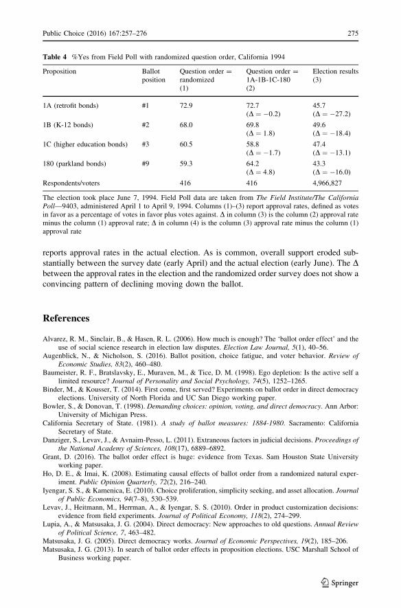
reports approval rates in the actual election. As is common, overall support eroded sub-

stantially between the survey date (early April) and the actual election (early June). The Dbetween the approval rates in the election and the randomized order survey does not show a

convincing pattern of declining moving down the ballot.

References

Alvarez, R. M., Sinclair, B., & Hasen, R. L. (2006). How much is enough? The ‘ballot order effect’ and theuse of social science research in election law disputes. Election Law Journal, 5(1), 40–56.

Augenblick, N., & Nicholson, S. (2016). Ballot position, choice fatigue, and voter behavior. Review ofEconomic Studies, 83(2), 460–480.

Baumeister, R. F., Bratslavsky, E., Muraven, M., & Tice, D. M. (1998). Ego depletion: Is the active self alimited resource? Journal of Personality and Social Psychology, 74(5), 1252–1265.

Binder, M., & Kousser, T. (2014). First come, first served? Experiments on ballot order in direct democracyelections. University of North Florida and UC San Diego working paper.

Bowler, S., & Donovan, T. (1998). Demanding choices: opinion, voting, and direct democracy. Ann Arbor:University of Michigan Press.

California Secretary of State. (1981). A study of ballot measures: 1884-1980. Sacramento: CaliforniaSecretary of State.

Danziger, S., Levav, J., & Avnaim-Pesso, L. (2011). Extraneous factors in judicial decisions. Proceedings ofthe National Academy of Sciences, 108(17), 6889–6892.

Grant, D. (2016). The ballot order effect is huge: evidence from Texas. Sam Houston State Universityworking paper.

Ho, D. E., & Imai, K. (2008). Estimating causal effects of ballot order from a randomized natural exper-iment. Public Opinion Quarterly, 72(2), 216–240.

Iyengar, S. S., & Kamenica, E. (2010). Choice proliferation, simplicity seeking, and asset allocation. Journalof Public Economics, 94(7–8), 530–539.

Levav, J., Heitmann, M., Herrman, A., & Iyengar, S. S. (2010). Order in product customization decisions:evidence from field experiments. Journal of Political Economy, 118(2), 274–299.

Lupia, A., & Matsusaka, J. G. (2004). Direct democracy: New approaches to old questions. Annual Reviewof Political Science, 7, 463–482.

Matsusaka, J. G. (2005). Direct democracy works. Journal of Economic Perspectives, 19(2), 185–206.Matsusaka, J. G. (2013). In search of ballot order effects in proposition elections. USC Marshall School of

Business working paper.

Table 4 %Yes from Field Poll with randomized question order, California 1994

Proposition Ballotposition

Question order =randomized(1)

Question order =1A-1B-1C-180(2)

Election results(3)

1A (retrofit bonds) #1 72.9 72.7(D ¼ �0:2)

45.7(D ¼ �27:2)

1B (K-12 bonds) #2 68.0 69.8(D ¼ 1:8)

49.6(D ¼ �18:4)

1C (higher education bonds) #3 60.5 58.8(D ¼ �1:7)

47.4(D ¼ �13:1)

180 (parkland bonds) #9 59.3 64.2(D ¼ 4:8)

43.3(D ¼ �16:0)

Respondents/voters 416 416 4,966,827

The election took place June 7, 1994. Field Poll data are taken from The Field Institute/The CaliforniaPoll—9403, administered April 1 to April 9, 1994. Columns (1)–(3) report approval rates, defined as votesin favor as a percentage of votes in favor plus votes against. D in column (3) is the column (2) approval rateminus the column (1) approval rate; D in column (4) is the column (3) approval rate minus the column (1)approval rate

Public Choice (2016) 167:257–276 275

123

Meredith, M., & Salant, Y. (2013). On the causes and consequences of ballot order effects. PoliticalBehavior, 35(1), 175–197.

Miller, J. M., & Krosnick, J. A. (1998). The impact of candidate name order on election outcomes. PublicOpinion Quarterly, 63(2), 291–300.

Mueller, J. E. (1969). Voting on propositions: Ballot patterns and historical trends in California. AmericanPolitical Science Review, 63(4), 1197–1212.

Selb, P. (2008). Supersized votes: ballot length, uncertainty, and choice in direct legislation elections. PublicChoice, 135(3/4), 319–336.

276 Public Choice (2016) 167:257–276

123