Banks’ Risk Exposures∗

Juliane Begenau

Stanford

Monika Piazzesi

Stanford & NBER

Martin Schneider

Stanford & NBER

October 2013

Abstract

This paper studies US banks’ exposure to interest rate and default risk. We

exploit the factor structure in interest rates to represent many bank positions as

portfolios in a small number of bonds. This approach makes exposures compa-

rable across banks and across the business segments of an individual bank. We

also propose a strategy to estimate exposure due to interest rate derivatives from

regulatory data on notional and fair values together with the history of interest

rates.

∗PRELIMINARY & INCOMPLETE. Email addresses: begenau@stanford.edu, pi-

azzesi@stanford.edu, schneidr@stanford.edu. We thank John Cochrane, Darrell Duffie, Isil Erel,

Bob Hall, Lars Hansen, Anil Kashyap, Jean-Charles Rochet, Chris Sleet, John Taylor, Harald Uhlig

and seminar participants at Arizona State, Chicago Booth Econometrics and Statistics Workshop,

Chicago Money & Banking, Duke, the 4th Banque de France—Bundesbank Conference in Paris, the

Conference in Honor of Sargent and Sims at the Federal Reserve Bank of Minneapolis, the Conference

on Expectational Coordination at the College de France, CREI, the Econometric Society Meeting in

Seoul, Federal Reserve Board, the Federal Reserve Banks of Chicago, San Francisco, and New York,

NYU, MIT, Ohio State, Princeton University, the ShovenFest at Stanford, SITE, Society of Economic

Dynamics in Cyprus, Stanford, Stanford Conference in Quantitative Finance, UC Davis, Yale and

Wharton.

1

1 Introduction

The economic value of financial institutions depends on their exposure to market risk.

A traditional bank borrows short term via deposits and lends long term via risky loans.

Modern institutions have increasingly borrowed short term in the money market, for

example via repurchase agreements and lent long term via holding securities such as

mortgage bonds. Modern banks also play a prominent role in derivatives markets. The

value of positions taken as a result of these activities changes if market prices change,

for example because of news about future monetary policy or default rates.

Measuring banks’ risk exposure is not only important for regulation, but also matters

for economic analysis more broadly. Institutions are the main players in markets for fixed

income instruments. For example, many short term instruments (such as commercial

paper) are not traded directly by households. Moreover, banks choose risk exposures that

are different from each other and therefore have different experiences when conditions

change (for example, Lehman versus JP Morgan during the 2007-2009 financial crisis.)

This has motivated a literature that aims to explain asset prices from the interaction

of heterogeneous institutions. To quantify such models, we need to know banks’ risk

exposures.

It is difficult to discern exposures from banks’ reported credit market positions. In-

deed, common data sources such as annual reports and regulatory filings record account-

ing measures on a large and diverse number of credit market instruments. Accounting

measures are not necessarily comparable across positions. For example, the economic

value of two loans with the same book value but different maturities will react quite

differently to changes in interest rates. At the same time, many instruments are close

substitutes and thus entail essentially the same market risk. For example, a 10 year

government bond and a 9 year high-grade mortgage bond will tend to respond similarly

to many changes in market conditions.

This paper constructs comparable and parsimonious measures of banks’ exposure to

market risk by representing their positions as portfolios in a small number of bonds.

We start from balance sheet data from the US Reports on Bank Conditions and Income

(“Call Reports”). We show how to construct, for any bank and for each major class of

credit market instruments, replicating portfolios of bonds that have approximately the

same conditional payoff distribution. We then compare portfolios across positions as

well as across banks.

Our findings suggest that the overall position of the major dealer banks is a portfolio

which is long in long-term bonds and short in cash. We also find that these banks have

large net positions in interest-rate derivatives. This net derivative position comes close

in magnitude to the net position in other fixed income business. We document that,

2

during much of our sample, the net-interest rate derivative position does not hedge other

balance-sheet positions. Instead, banks increase their risk exposure through derivatives.

Because of its large size, it is important to account for the net position in interest-rate

derivatives when measuring exposure. The key difficulty in measuring the exposure in

interest-rate derivatives is that banks do not report the sign of their position — whether

they represent bets on interest rate increases (e.g., pay-fixed swaps) or decreases (e.g.,

pay-floating swaps.) Moreover, there is no detailed information about the maturities of

these net (as opposed to gross) derivatives positions or the start day of these derivatives

(and thus their associated locked-in interest rates).

To deal with the lack of reported information, we propose a novel approach to obtain

the exposure contained in the net position in interest-rate derivatives. We specify a state

space model of a bank’s derivatives trading strategy. We then use Bayesian methods to

estimate the bank’s strategy using the joint distribution of interest rates, bank fair and

notional values as well as bid-ask spreads. Intuitively, the identification of the bank’s

strategy relies on whether the net position (per dollar notional) gains or loses in value

over time, together with the history of rates. If rates go up and the bank’s derivative

position experiences gains, the Bayesian estimation puts more probability on a derivative

position with a pay-fixed interest rate.

Our approach is motivated by the statistical finding that the market value of fixed

income instruments exhibit a low-dimensional factor structure. Indeed, a large literature

has documented that the prices of many types of bonds comove strongly, and that these

common movements are summarized by a small number of factors. It follows that for any

fixed income position, there is a portfolio in a few bonds that approximately replicates

how the value of the position changes with innovations to the factors.

For loans and securities, the replication portfolio is derived from detailed information

on the maturity distribution provided by the call reports. For loans reported at book

value, we follow Piazzesi and Schneider (2010) and represent loan portfolios as bundles

of zero coupon bonds. For securities reported at market value, we use those market

values together with the properties of zero coupon bond prices. For derivatives, the

replication portfolio becomes an observation equation for a state space system, which

has unobservable replication weights that can be estimated.

Related literature

The current regulatory framework is known as Basel II. The regulation distinguishes

between credit risk due to borrower default and market risk due to price changes. Reg-

ulator ask banks to estimate default probabilities of the securities that they are holding

either with (external) credit ratings or with internal models. Based on the default proba-

bilities, regulators compute capital requirements for the various positions. This approach

3

treats the positions one by one. Our portfolio approach treats credit and market risk

jointly — exploiting the fact that borrowers tend to default when prices move and vice

versa. Moreover, we make positions comparable with each other.

A popular approach to measuring the interest-rate risk exposure of a bank is to run

regressions of the bank’s stock return on a risk factor, such as an interest rate. The

regression coefficient on the interest rate — often referred to as the interest-rate beta, is a

measure of the bank’s average exposure to interest rate changes over the sample period

considered (Flannery and James 1984a). More recently, Landier, Sraer and Thesmar

(2013) take the left-hand side variable to be changes in interest income or earnings as

a fraction of assets. Interest rate betas do not tell us where the bank’s exposure comes

from, that is, what positions generate it. This issue has been investigated by relating

interest rate betas to summary statistics of bank positions. For example, interest rate

betas have been related to banks’ maturity gaps, that is, the difference between bank

assets and liabilities that mature within a specified horizon (Flannery and James 1984b).

Moreover, changes in bank equity values have been related to off-balance sheet statistics

that indicate derivative use (Venkatachalam 1996). A key feature of this line of work

is that exposure measures are by construction constant over time and cannot speak to

how exposures change. Recent extension have attempted to incorporate time-varying

interest rate betas, but those have proven difficult to estimate (for example, Flannery,

Hammed, and Haries 1997, Hirtle 1997). Our replication approach is designed to provide

time series of exposure. Moreover, since we work with positions data, we can report for

each date what positions are generating what exposure.

Our Bayesian approach estimates a time-varying exposure from banks’ gains and

losses on their interest-rate derivative positions. This approach builds on early work by

Gorton and Rosen (1995) who did not have data on market values, because few banks

reported them before the adoption of fair value accounting in the mid 1990s. Instead,

Gorton and Rosen use data on "replacement costs" from the Call Reports, which refers

to the value of derivatives that are assets to the bank (not netting out the liabilities).

Under the assumption that the positions have constant maturity and constant interest-

rate exposure, these data can be used to compute the market value of interest-rate

derivatives.

We find that banks mostly take pay-floating positions in interest-rate derivatives,

which are positions that gain in value from a surprise fall in interest rates. Some of the

counterparties to these positions are nonfinancial corporations, who use pay-fixed posi-

tions in swaps to insure themselves against surprising interest-rate increases. Hentschel

and Kothari (2001) and Chernenko and Faulkender (2011) document these positions em-

pirically. Jermann and Yue (2012) use a theoretical framework to understand why non-

financial corporations have a need for pay-fixed swaps. Minton, Stulz, and Williamson

4

(2009) document which financial corporations use credit derivatives.

Since the financial crisis, there has been renewed interest in documenting the balance-

sheet positions of financial institutions. We share the important goal of this literature:

to come up with data on positions that will inform the theoretical modeling of these insti-

tutions, as called for by Franklin Allen in his 2001 AFA presidential address. Adrian and

Shin (2011) investigate the behavior of Value-at-Risk measures reported by investment

banks. They document that VaR per dollar of book equity stayed constant throughout

the last decade, including the financial crisis, when these institutions were deleverag-

ing. He, Khang, and Krishnamurthy (2010) document the behavior of book values of

balance sheet positions of various financial institutions. These positions do not include

derivatives.

Our estimated exposures in the form of replicating portfolios provide broad risk mea-

sure for financial institutions. Other risk measures focus on tail risk (e.g., VaRs, Acharya,

Pedersen, Phillipon, and Richardson 2010, Kelly, Lustig, and van Nieuwerburgh 2011)

or on stress tests (Brunnermeier, Gorton, Krishnamurthy 2012, Duffie 2012). The ad-

vantage of replicating portfolios is that they describe the entire distribution, not just

tail risks or individual scenarios. Moreover, our portfolios are additive, so that they can

be compared across positions within a bank as well as across banks.

2 Banks’ fixed income portfolios

Our goal is to understand financial institutions’ fixed income strategies. In particular,

we would like to compare strategies across institutions and relate different components of

an individual institution’s strategy, such as its loan portfolio and its derivatives trading

business. To characterize the risk exposure of these strategies, we want to describe the

period portfolio holdings and their loadings on one-step risks. We are thus interested

in measuring the entire one-step ahead conditional value distribution of these portfolios.

To do that, we fix a probability space (∞ P). Here is the state space: oneelement ∈ is realized every period. Denote by the history of state realizations.

It summarizes all contingencies relevant to institutions up to date including not only

aggregate events (such as changes in interest rates), but also events specific to an indi-

vidual institution, such as changes in the demand for loans and deposits, or the order

flow for swaps.

We think of a fixed income instrument as a history-contingent payoff stream that

is denominated in dollars. The simplest example is a safe zero coupon bond issued at

some date that pays off one dollar for sure at the maturity date + say. More

generally, payoffs could depend on interest rates — for example, an interest rate swap

5

or an adjustable rate mortgage promise payoff streams that move with a short term

interest rate — or on other events, such as customers’ decisions to prepay or default on

a mortgage.

We assume that every instrument of interest can be assigned a fair value. Following

GAAP accounting rules, we view the fair value as the price at which the instrument

could be sold “in an orderly transaction”. For instruments traded in a market, fair

values can be read off market prices. For nontraded instruments, such as loans, fair

values have to be constructed from the payoffs of comparable instruments.

The starting point for our analysis is the fact that fair values of fixed income instru-

ments tend to move together. In particular, the overwhelming majority of movements in

bond prices is due to the “overall level” of interest rates. The latter can be summarized

by any particular interest rate, for example a riskless nominal short rate. Since fixed

income instruments are fairly predictable payoff streams, it is natural that changes in

discount rates drive their value. For bonds that are issued by borrowers in the private

sector (such as mortgages or business loans), default risk is also very important. To

describe the movements of private sector bond prices, it is thus important to capture

changes in credit risk.

We thus assume that fair values of all relevant fixed income instruments can be

written as functions of calendar time and a small number of random variables that we

refer to as factors. Let denote a ( × 1)-vector-valued stochastic process of factors.Here each is a random variable that depends on the history

but we mostly suppress

this dependence in what follows.

The fair value ( ) of a fixed income instrument depends on the factors and

calendar time , which is important because the maturity date is part of the description

of the payoff stream. As an example, let the payoff stream correspond to a riskfree zero

coupon bond with maturity date + that was issued at date or earlier. Let ()

denote the yield to maturity on an -period zero coupon bond quoted in the market

at date . The price at date is exp(−() ). At any later date + before maturity

date (so ), the price is exp(−(−)+ (− )). The payoff stream thus satisfies our

assumption as long as the interest rate depends on the factors.

We assume further that the distribution of the factors is given by a process with a

conditional Gaussian distribution. We thus represent the distribution of under P bya process that satisfies

+1 v N¡ ( )

2

¢(1)

with a conditional mean that depends on the factor and a volatility that may depend

on time to capture time-varying uncertainty. We assume that the riskless one period

6

interest rate is a linear function of the factors:

= 0 + >1

We approximate the change in the fair value of the instrument as a linear function

in the shocks +1. If time were continuous, Ito’s lemma would deliver this result

exactly, given conditional normality and the smoothness of the value . Here we use a

second-order Taylor expansion and the properties of normal distributions. We write

(+1 + 1)− ( ) ≈

( ) (+1 − ) +

( ) +

1

2

2

>( )

>

=: + (+1 − ( )) (2)

where the first (approximate) equality uses the fact that the third moments of a normal

distribution are zero and higher moments are an order of magnitude smaller than the

first and second moments. The coefficient is the expected change in fair value. If we

divide by the current fair value, ( ), we get the expected return. The 1× slope

coefficients is the exposure of the fair value to the factor risks, +1

We are now ready to replicate the payoff stream of any instrument by + 1 simple

securities. That is, we define, for each date a portfolio of + 1 securities that has

the same value as the instrument in every state of the world at date + 1. We always

take one of the securities to be the riskless one period bond; let 1 denote the number

of short bonds in the portfolio at date . Since 1 is also the face value of the one-period

riskless bonds, we will refer to 1 as cash. For the payoff stream corresponding to a short

bond, the coefficients in (2) are given by = − and = 0. Consider additional

“spanning" securities that satisfy

+1 − = + +1 (3)

The × 1 vector denotes the holdings of spanning securities at date . In our onefactor implementation below the only spanning security will be a long bond (so that will be a scalar).

For each period we equate the change in the value of the position and its replicating

portfolio. This means that for every possible realization of the shocks +1, the holdings

of cash 1 and spanning securities solve

¡

¢µ 1

+1

¶=³1

>

´µ − 0

¶µ1

+1

¶ (4)

These are +1 equations in +1 unknowns, the holdings³1

>

´of cash and longer

spanning bonds. If the matrix on the left hand side is nonsingular then we can find

portfolio holdings (1 > ) that satisfy this equation.

7

If the market prevents riskless arbitrage, then the value of the replicating portfolio

at date should be the same as the value of the payoff stream ( ). Suppose to the

contrary that the value of the replicating portfolio, b ( ) say, was lower than ( ).

Then one could sell short one unit of the payoff stream buy one unit of the replicating

portfolio and invest the difference b ( )− ( ) in the riskless asset. Since the changein value for and the replicating portfolio is identical, this strategy delivers a riskfree

profit that consists of the interest earned on b ( )− ( ). It follows that one periodahead a position in the payoff can be equivalently viewed as a position in the replicating

portfolio: it has the same value at date as well as in each state of the world at date

+ 1 Alternatively, we can divide equation (4) by the value b ( ) = ( ) and see

that the returns on these two strategies are equalized state by state.

Once positions are represented as portfolios, we can measure risk by considering how

the value of the position changes with the prices of the long term spanning securities

, or equivalently with the factor innovations +1. If the short interest rate is the only

factor, then the exposure of the position is closely related to duration, which is defined

as (minus) the derivative of a bond’s value with respect to its yield. In this case, the

holdings of the spanning bonds are the delta of the position, and the change in value

(4) can be used for Value at Risk (VaR) computations that determine the threshold loss

that occurs with a certain probability. For example, we might determine that a given

bond has a one-quarter 5% VaR of 90 cents. This would correspond to a 5% probability

that the bond’s price will fall by more than 90 cents over the quarter.

The advantage of the portfolio representation (4) over VaR is that it fully describes

the conditional distribution of risk in the instrument, not just the probability of a certain

tail event. Another advantage is that the replicating portfolios of various fixed-income

positions are additive, making these positions easy to compare. The same is not true for

VaR computations of complex positions. Moreover, our approach can easily incorporate

factors in addition to the short rate, such as liquidity factors.

2.1 Data on fixed income portfolios

Our data source for bank portfolios are the Bank Reports of Conditions and Income,

or "call reports”, filed quarterly by US commercial banks and bank holding companies

(BHCs). The call reports contain detailed breakdowns of the key items on an institution’s

balance sheet and income statement. The breakdowns are for most items more detailed

than what is contained in corporations’ SEC filings for banks. At the same time, the call

reports contain all banks, not simply those that are publicly traded. They also contain

additional information that helps regulators assess bank risk. Of particular interest to us

are data on the maturity distribution of balance sheet items such as loans and borrowed

8

money, as well as on the notional value and maturity of interest rate derivative contracts.

Table 1 shows the balance sheet for JP Morgan in year 2011. JP Morgan has 2.3

Trillion Dollars of total assets and liabilities in 2011. Much of its balance sheet is

traditional bank business. For example, half of its liabilities are deposits and a third of

its assets are loans and some cash. JP Morgan also borrows 10% from other banks in

the Federal Funds Market and lends out 17% of its assets to other banks. The more

modern bank business is contained in the 16% securities and 20% trading assets. These

positions contain a myriad of fixed-income securities that are traded on markets. For

example, Appendix A shows Schedule HC-B for securities which include Treasuries, U.S.

agency bonds, bonds issued by states and municipalities, mortgage-backed securities,

asset-backed securities, and other structured financial products.

Table1: JP Morgan0s Balance Sheet in Year 2011Assets Liabilities

Cash 6% Deposits 50%

Securities 16% Other borrowed money 15%

Trading assets 20% Trading liabilities 6%

Fed funds + Repos 17% Fed funds + Repos 10%

Loans 31%

Other assets 10% Other liabilities 11%

Equity 8%

The trading assets contain assets for which JP Morgan is a market maker, such as

Treasuries. It also contains derivatives. These are mostly interest-rate derivatives. The

lion share of these interest-rate derivatives are swaps; JP Morgan has 60 Trillion Dollars

of swap notionals. We want to understand the net exposures in these various types of

positions.

Figure 1 gives a first impression of the value of the various positions over time. The

dotted dark blue line shows the net fair value of interest rate derivatives. The value seems

smaller in magnitude compared to the solid dark blue line, which measures its traditional

fixed income business: loans plus securities plus trading assets less deposits and other

debt. To put these numbers in perspective the red line is (book) equity over assets.

Finally, the light blue line labeled "net other" is a residual defined so that all three blue

lines together add up to equity. The remainder of this paper is about understanding the

risk exposure inherent in the leveraged fixed income positions represented by the dark

blue lines (both dotted and solid.)

The net fair values in Figure 1 are not very informative about the risk exposure in

these positions. For example, if JP Morgan enters a pay-floating swap contract, its net

9

1995 2000 2005 2010

−2

0

2

4

6

8

% a

sset

s

net fixed incomenet i.r. derivsequitynet other

Figure 1: Balance sheet positions of JP Morgan Chase

fair value in interest-rate derivatives is zero (up to bid-ask spreads.) This position still

represents a leveraged bet on future interest rate declines which will gain in value with

a surprise rate drop. More formally, the fair values represent the overall value of their

replicating portfolio

( ) = 1 − +

>

To learn about the risk exposure of the portfolio, we would need to know the portfolio

weights ()

() ( ) on each of the = 1 risky spanning securities and how

these weights change over time. In particular, these portfolio weights may involve large

long-short positions that involve large exposures to risk factors +1 but with an overall

small fair value ( ) The spanning securities depend on the risk in the factors +1through the loadings in equation (3). Therefore, once we know the portfolio weights

for each period , we know how the portfolio depends on the risk factors. The rest of

the paper will compute the replicating portfolio³1

>

´for each U.S. bank.

10

3 A Portfolio View of Bank Call Reports

In this section we replicate major bank positions in the call reports by portfolios in two

“spanning” zero coupon bonds — a one quarter bond (which we often refer to as "cash")

as well as a five year bond. Zero coupon bonds are useful because most instruments can

be viewed as collections of such bonds, perhaps with adjustments for default risk. For

example, a loan or a swap can be viewed as collection of zero coupon bond positions of

many different maturities — one for every payment. We now describe a pricing model

that gives rise to a linear representation of fair values as in (2) as well as the pricing of

zero coupon bonds for that model.

3.1 Summarizing interest rate dynamics

We consider an exponential affine pricing model that describes the joint distribution of

riskfree nominal government bonds and risky nominal private sector bonds. The nominal

pricing kernel process +1 represents one step ahead dollar state prices (normalized by

conditional probabilities) for dollar payoffs contingent on the factor innovation +1. In

particular, for any payoff ( +1 ()) the date price is [+1 (

+1) ( +1 ()) |].

We choose the functional form

+1 = exp

µ− − 1

2> − > +1

¶(5)

= 0 + 1

The price of a certain payoff of one is the one period zero coupon bond price (1) =

exp (−). Consider next the risky payoff exp (+1 − 12): it has mean one and itsprice is exp (− − ). We can interpret as the price discount induced by risk

contained in the th innovation +1 — it is often referred to as the “market price” of

the risk introduced by that innovation. Equivalently, it represents the expected excess

return, or risk premium, on the risky payoff. These risk premia can in general vary over

time with the factors.

We assume that the factor dynamics (1) are an AR(1), so that

( ) =

The autoregressive parameter and the factor volatility may dependend on calendar

time in some of our estimations below as well as the risk premia parameters 0 and 1

To keep the notation in this section simple, we will omit this time dependence.

11

Riskfree government bonds

The price of an -period riskless zero coupon bond is given recursively by (0) = 1

()

¡¢=

h+1

¡+1

¢(−1)+1

¡ +1

¡¢¢ |i

For = 1, this equation just restates the definition of the one period bond price (1)

More generally, the one-period-ahead payoff of an -period zero coupon bond is the

price of the bond next period, when the bond has matured to have maturity − 1.Our functional form assumptions ensure that all prices take the form

() = exp

¡ +>

¢

(6)

where the coefficients and satisfy a system of difference equations. Log prices are

therefore affine in the factors. This property is convenient when computing log returns:

for example the one period holding return on the -period bond log(−1)+1 − log ()

is affine in +1 and .

The difference equations for the coefficients and are given by the system

+1 = −>0 +

1

2>

> − 0

>+1 = >

(− 1)− >1

with boundary conditions 1 = −0 and 1 = −1 (Ang and Piazzesi, 2003).The recursion illustrates how the model incorporates the expectations hypothesis of

the term structure. Indeed, consider first risk neutral pricing ( = 0). The Jensen’s

inequality terms involving the variance > tend to be small relative to the other terms.Up to Jensen terms, we can write the log price as minus the sum of expected future

short rates

log() = −0− 1

X=0

+ Jensen term = −

X=0

(1)+ + Jensen term.

Roughly speaking, long-term interest rates () = − log () are then short-term

interest rates that are expected to prevail over the lifetime of the bond. The coefficient

recursion for and computes this expectation since the factor has AR(1) dy-

namics. With risk adjustment, the mechanics remain the same; the only difference is

that expectations are taken under a risk-adjusted probability. After risk adjustment,

expectations are formed using different AR(1) coefficients − 1 for the factors and a

different long-run mean (−0 rather than 0.)

12

The affine model leads to simple formulas for the coefficients and in (2):

(−1)+1 −

() ≈

()

µ>−1 (+1 − ) +−1 − + (−1 −)

> +

1

2>−1

>−1

¶=

()

µ>−1 (− 1) +−1 − + (−1 −)

> +

1

2>−1

>−1

¶+

() >

−1+1

= ()

¡ +>

−1 +>−1+1

¢(7)

= + +1

where the second equality uses the coefficient difference equations.

After dividing the expected change in the bond price (7) by the current price of the

bond () , we can see that the expected excess returns on a riskfree -period bond held

over one period is >−1. The amount of risk in the excess return on a long bond is

>−1, which is a vector describing the amount of risk due to each of the shocks +1.The vector of market prices of risk captures a contribution to expected excess returns

that is earned as a compensation for a unit exposure to each shock.

Suppose that there is a single factor ( = 1) which is positively related to the riskless

short rate, that is 1 0. A large positive shock +1 means an increase in the short rate,

which lowers the one-period bond price (1)+1. If 0, a higher short rate represents a

bad state of the world. The reason is that, with a negative , the pricing kernel +1

depends positively on +1.Since bond prices are exponential-affine (6) and the coefficient

−1 is negative, they have low payoffs in bad states and are thus unattractive assets toinvestors. To hold such assets, investors want to be compensated with positive expected

excess returns. In other words, on average >−1 is positive.

The conditional standard deviation of the return on the long-term bond is (approxi-

mately) equal to−−1. This suggests an alternative interpretation of − in equation(7) as the (positive) Sharpe ratio of the bond, its expected excess return divided by the

return volatility. The Sharpe ratio is positive if long bonds have low payoffs in bad states

— in which case they are unattractive assets that need to compensate investors with a

positive premium.

Risky private sector bonds

Private sector bonds are subject to credit risk. For each dollar invested in risky

bonds between and + 1, there is some loss from default. We treat a risky bond as a

claim on many independent borrowers, such as a mortgage bond or an index of corporate

bonds. For every dollar invested in the risky bond at date , there will be some loss from

13

default between dates and +1 due to the law of large numbers. This loss will depend

on the pool of borrowers and, in particular, their credit rating. For example, a pool

of junk-rated borrowers will generate higher expected losses than a pool of AAA-rated

borrowers. Moreover, the loss can be larger or smaller depending on the state of the

economy at date , captured by the factors , as well as the state of the economy at

date + 1, captured by +1 (or equivalently, given knowledge of by the innovation

+1).

To retain the tractability of the affine model, we follow Duffie and Singleton (1999)

and assume that the recovery value on a bond in default is proportional to the value

of the bond. In particular, suppose () is the value of an -period zero coupon risky

bond trading at date with a certain credit rating. As of date , investors anticipate the

value of the bond at + 1 to be ∆+1(−1)+1 , where the loss factor

∆+1 = exp

µ− ( − )− 1

2

³> − >

´−³ −

´>+1

¶captures jointly the probability of default and the recovery value. We assume that the

risky rate is linear and the process is linear as well

= 0 + >1

= 0 + 1

Each credit rating will have its own associated group of parameters 0 1 0 and 1

The prices of risky bonds are determined recursively as risk adjusted present values:

()

¡¢=

h+1

¡+1

¢∆+1

¡+1

¢(−1)+1

¡ +1

¢ |iAs for riskless bonds, there is an exponential affine solution solution

() = exp

³ + >

´

where and satisfy a system of difference equations

+1 = − >0 +

1

2>

> − 0

>+1 = >

³− 1

´−

>1 (8)

with boundary conditions 1 = −0 and 1 = −>1 The exposures of bond prices

to the factor will vary across credit ratings.

14

The expected excess return on a risky short bond is

log∆+1 +1

2 (log∆+1)− log (1) − = −>

³ −

´With risk neutral pricing, the right-hand side is zero. Therefore, the spread between

risky and riskfree interest rate − reflects only the expected loss per dollar invested

which can vary over time with . More generally, the spread can be higher or lower than

the risks-neutral spread because of risk premia. In particular, 0 means that high

factor realizations are a bad state of the world (so that +1 is high when +1 is large.)

If losses per dollar invested are higher when the factor is high, risky bonds have low

payoffs in bad states. Investors then demand a positive expected excess return on the

one-period risky bond over the short rate. Whether or not losses are high when interest

rates are high depends on how payoffs ∆+1 depend on +1 If , high +1 leads

to high losses and thus low payoffs ∆+1. In this case, investors want positive expected

excess returns, which we can also see from the right-hand side of the equation.

Replication of risky zero coupon bonds

The affine model leads to simple formulas for the coefficients and in (2) if the

payoff stream is a risky zero coupon bond. Taking default into account, the change in

the portfolio value between and + 1 is

∆+1(−1)+1 −

() ≈

()

³− ( − ) + −1 + >

−1 (− 1) −

´+

()

µ³−1 −

´> +

1

2>−1

>−1

¶+

()

µ>−1 −

³ −

´>¶+1

= ()

µ +

µ>−1 −

³ −

´>¶ +

µ>−1 −

³ −

´>¶+1

¶= + +1

where again the first equality uses the coefficient difference equations.

Note that the parameters 0 and 1 affect the replication of the change in value only

through the coefficients −1 and −1. This is because they represent predictablelosses from default which affect the value of the risky position, but not its change over

time. The coefficient ()

() is the expected return on the risky bond, which is

equal to the riskless short rate plus the risk premium

µ>−1 −

³ −

´>¶ The

risk premium has two terms as it compensates investors for both time variation in the

bond price at + 1 as well as the default loss between and + 1. For the riskless

15

bond, this risk premium is just equal to >−1 as computed above. The coefficientµ

>−1 −

³ −

´>¶

() is the volatility of the return on the bond between and

+ 1. In the one factor case, the market price of risk is again the Sharpe ratio.

Replication with a single factor

Suppose we have a single factor, so that we can replicate any instrument using cash

1 and a public bond with spanning maturity . To replicate a private bonds with

maturity , we equate the changes in value

(1) 1 +

() ( +−1 ( + +1)) =

()

³ +

³−1 −

³ −

´´( + +1)

´

The replicating portfolio weight is given by

()

()

=−1 −

³ −

´−1

on the -period public bond. To translate this portfolio weight into holdings we

also match the value () An important feature of the portfolio weight is that it can be

computed entirely with risk-adjusted parameters. These parameters that determine ,

, , and can be estimated from repeated cross sections of bonds for every period

separately. This allows the procedure to accommodate changes in risk over time as

well as in risk premia parameters 0 1 0 and 1 Below, we will report results for both

the case where these parameters are constant and for the case where the parameters

change over time.

If the bond we are replicating is riskless, the portfolio weight is constant over time

and has the simpler formula

()

()

=−1−1

Intuitively, if = , the portfolio weight is equal to 1. Moreover, the s are negative

and their absolute value increases in maturity, so we will find a larger portfolio weight

if and smaller otherwise. If = 1, then 0 = 0 and the portfolio weight on the

long riskless bond is zero, because the replicating portfolio consists only of cash.

A risky, private sector bond is like a riskless bond with a different duration. Whether

it is shorter or longer depends on the parameters of ∆. There are two effects. First,

the replicating portfolio captures exposure to the interest rate induced by losses from

default between and + 1. The direction of this effect depends on the sign of −

If , then there is more default (or a lower payoff in default) when interest rates

16

are high. As a result, a riskier bond will have more exposure to changes in interest rates

and is thus more similar to a longer riskless bond.

The second effect comes from the difference between the coefficients and . From

(8), this effect depends not only on 1, but also on 1. If 1 1, then there are larger

expected losses from default if interest are high. This means that risky bond prices are

more sensitive to interest rates than riskless bond prices of the same maturity, so that

again risky bonds work like longer riskless bonds. The opposite result obtains if 1 1.

3.2 The estimated one factor model

We estimate the government and private sector yield curves using quarterly data on

Treasury bonds, swap rates and corporate bond rates over the sample 1995:Q1-2011:Q4.

We have data on corporate bonds with 14 different credit ratings: AAA, AA, A+, A,

A−, BBB+, BBB, BBB−, BB+, BB, BB−, B+, B and B−. Swap contracts are notmuch affected by credit risk because of collateral provisions. The floating side of the

swap is set to LIBOR, which does reflect the credit risk of banks. As a result, swap rates

are very close to AAA-rated bond yields.

The government bond yields are the solid lines in Figure 2, while swap yields with

the same maturity are the dashed lines in the same color. In a principle component

analysis, a large fraction of the variation in these yield data, 93%, is explained by a single

factor. In Figure 2, this is reflected by the fact that all rates vary around together. The

movements in the longer maturity rates (towards the top in the figure) are somewhat

dampened versions of the movements in the shorter maturity interest rates (towards the

bottom.) The gray shaded area is the TED spread, defined as the difference between

the 3-month LIBOR rate and the 3-month T-bill rate. This spread is higher in times

when interest rates are high—right before recessions. This is why these credit spreads are

commonly used as leading recession indicators. During the financial crisis of 2007-2008,

the TED spread increased further when interest rates fell unexpectedly.

As our single factor, we choose the BB-rated interest rate, which will capture both

interest rate risk as well as credit risk. To measure the exposure of public and pri-

vate bonds to changes in this risky rate, we need (i) its time series dynamics (1), (ii)

coefficients that describe the dependence of short public (0 1) and private³0 1

´short-term rates depend on the factor and (iii) coefficients that capture risk premia for

public (0 1) and private bonds³0 1

´.

The estimation of the government yield curve is in several steps. First, we estimate

the parameters and with OLS on the (demeaned) factor dynamics (1). Then we

estimate the parameter 0 as the mean of the riskless short rate and 1 with an OLS

17

1995 2000 2005 2010

0

2

4

6

8pe

rcen

t p.a

.

TED3m Libor1y swap2y swap3y swap5y swap10y swap

Figure 2: Public and private sector zero-coupon interest rates with the same maturity.

Solid lines are public, dashed lines are private. The gray shaded area is the TED spread,

which is the difference between the 3-month libor rate and the 3-month Treasury bill

rate.

regression of the short rate on the factor. Finally, we estimate the parameters 0 and 1by minimizes the squared errors from the model

min01

X

³() −b()

´2(9)

where b() = −

− >

For every credit rating, we also estimate a group of parameters 0 1 0 and 1. The

coefficients 0 and 1 are obtained with an OLS regression of the short credit-risky rate

18

on the demeaned factor. The estimates of the parameters 0 and 1 minimize the squared

errors

min01

X

³() − b()

´2(10)

where the model-implied private yields are

b() = −

− >

For the portfolio weights, it is enough to estimate the risk-adjusted parameters. We

do this by solving the nonlinear-least squares problems (9) and (10) for every period

separately We also tried estimating the factor dynamics and the ( ) parameters for

each period. These estimations did not give portfolio weights that differed much from

what we report below.

Panel A in Table 2 contains the estimation results together with Monte Carlo stan-

dard errors. The parameter 0 times four is the average short rate, 3.08%. The riskless

short rate has a loading below one on the factor, 1 = 086 The factor is highly per-

sistent with a quarterly autoregressive coefficient of 0.92. The market prices of risk are

on average negative, 0 = −029 (since the factor has a mean of zero), implying thathigh nominal interest rates represent bad states of the world. Investors want to be com-

pensated for holding assets — such as private or public nominal bonds — that have low

payoffs (low prices) in those states. These average prices of risk are, however, impre-

cisely estimated in small samples. The market prices of risk are significantly smaller

(“more negative”) in bad times, 1 = −27 In other words, risk premia are significantlycountercyclical.

Losses per dollar invested in risky bonds are estimated to be larger when the factor

realization is large Therefore, investors demand compensation for holding risky

bonds; expected excess returns on risky bonds are positive. Spreads between risky and

riskless rates covary positively with the level of interest rates—as suggested by the large

TED spread during periods of high rates in Figure 2.

Panel B in Table 2 shows average absolute fitting errors between 45 basis points and

up to 1.19 percentage points. With one factor that captures both the level of interest

rates and credit risk, the estimation distributes these errors across the various maturities

and credit ratings. Since the factor is the BB-rated short rate, the errors are largest for

the safest bonds, which have short maturities and higher credit ratings.

19

Table 2: Yield Curve Estimations

Panel A: Parameter estimates

Factor dynamics 0.9153 0.0016

(0.0053) (0.0001)

0 1 0 1public yields 0.0077 0.8648 −02940 −277352

(0.1425) (0.1153) (0.9836) (7.1847)

private yields 0 1 0 1swaps 0.0090 0.9851 −02392 −188120

(0.1623) (0.1452) (0.9808) (9.4895)

A-rated 0.0095 1.0103 −02697 −168991(0.1665) (0.1385) (0.9813) (9.0964)

BBB-rated 0.0106 0.9704 −02802 −185919(0.1599) (0.1616) (0.9816) (9.3845)

Panel B: Mean absolute errors (% per year)

maturity (in qrts) 1 4 8 12 20 40

public yields () 1.19 1.31 1.25 1.15 0.95 0.72

private yields ()

swaps 1.19 1.25 1.16 1.07 0.93 0.80

A-rated 1.04 1.07 1.00 0.86 0.70 0.51

BBB-rated 0.78 0.83 0.77 0.65 0.54 0.45

Note: Panel A reports parameter estimates and small sample standard er-

rors. The data are quarterly zero coupon yields from Treasuries, swaps, and

corporate bond rates with AAA, AA, A+, A, A-, BBB+, BBB, BBB-, BB+,

BB, BB-, B+, B and B-.ratings for the sample 1995:Q1-2011:Q4. The single

factor is the BB-rated short rate. The sequential estimation procedure is

described in the text. The small sample standard errors are computed from

10,000 Monte Carlo simulations with the same sample length as the data.

Panel B reports mean absolute fitting errors for public interest rates () and

private rates () for the indicated credit rating in annualized percentage

points.

20

3.3 Bank sample

Our analysis considers domestic top-tier bank holding companies (BHC) during 1995:Q1-

2011:Q4. Call Reports are filed by both for bank holding companies (BHC) and com-

mercial banks. A commercial bank is often owned by a BHC and a.BHC itself can be a

subsidiary of a larger BHC. We consider only BHCs that are the "top tier" company in

their BHC, and eliminate any BHC that is owned another BHC. We also eliminate all

BHC that have a foreign parent.

Most of the data series we are interested in are available directly at the consolidated

BHC level. However, for some series, in particular for positions on loans, securities

and borrowed money broken down by maturity, detailed information is available only

at the commercial bank level. To use this information, we match commercial banks to

their top tier parent BHC. We then aggregate positions by maturity over all commercial

banks with the same parent. We verify that total positions from bank and BHC files

are consistent.

We use information on merger and acquisition activities over our sample from the

Federal Reserve Bank of Chicago. This data has date of merger, the identity number of

the non-surviving and the acquiring bank and their respective bank holding company

identity number.

3.4 Loans and securities

The major categories of fixed income instruments on the asset side of the bank balance

sheet are cash, loans and securities. In order to arrive at a portfolio representation, we

first express balance sheet positions in terms of zero coupon bonds. For example, an

installment loan is as a bundle of many zero coupon bonds — one for each installment —

each with a credit rating derived from the risk weight assigned to the loan in the Call

Report. We now describe how data on balance sheet positions, interest rates, maturities

and risk weights is used for this step.

Accounting data

Under traditional accounting rules, loans and securities are recorded on balance

sheets at face value. The face value of a loan is usually the amount of money dis-

bursed when the loan is taken out (although there can be small differences, for example,

when a mortgage borrower buys points.) The face value of a securitiy position is the par

value of the security. Recent statements by the Financial Accounting Standard Board

(FASB) have moved US GAAP rules towards marked-to-market (MTM) accounting.

Statement FAS 115, issued in 1993, introduced a three way split of positions into

21

"held to maturity" (HTM), "available for sale" (AFS), and "held for trading" instru-

ments. The latter two categories are recorded at fair value on the balance sheet, while

HTM instruments are recorded at face value.1 The call reports provide a breakdown

into the three categories for both loans and securities. Over our sample, the majority of

positions in loans is recorded at face value, while the majority of positions in securities

is recorded at fair value.

Maturity data in the call reports are in the form of maturity (or repricing) buckets.

The five buckets contain positions of maturity less than one quarter, 1-4 quarters, 1-

3 years, 3-5 years, 5-15 years and more than 15 years. The call reports also provide,

for both loans and securities, risk weights that are used to calculate risk-based capital

requirements. Guidelines for filling out call reports relate risk categories to credit ratings.

Short term assets

For short term assets and liabilities, book value and fair value are typically very

similar. Here “short term” refers not to the maturity date, but rather to the next

repricing date. For example, a 30 year adjustable rate mortgage that resets every quarter

will also have a fair value close to its book value. We treat all assets with repricing date

less than one quarter as a one quarter bond, applying a private sector or government

short rate depending on the issuer.

Loans

We view loans as installment loans that are amortized following standard formulas.

We derive a measure of market value for loans by first constructing a payment stream

corresponding to a loan portfolio, and then discounting the payment stream using the

yield curve. The resulting measure is not necessarily the market price at which the bank

could sell the loan. Indeed, banks might hold loans on their portfolios precisely because

the presence of transaction costs or asymmetric information make all or parts of the

portfolio hard to sell. At least part of the loan portfolio should thus best be viewed as a

nontradable “endowment” held by the bank. Nevertheless, our present value calculation

will show how the economic value of the endowment moves with interest rates.

The first step is to find, for each date , the sequence of loan payments by maturity

expected by the bank. Let denote the loan payment that the expected as of date

by the bank in + , () To construct payment streams, we use data on the maturity

distribution of loan face values ( ) together with the yield to maturity on new loans

by maturity ( ). For the first period in the sample, we assume that all loans are new.

We thus determine the payments ( ) by a standard annuity formula: must equal

1The difference between AFS and trading assets is how changes in fair values affect earnings: trad-

ing gains and losses directly affect net income, whereas gains and losses on AFS assets enter other

comprehensive income (OCI), a component of equity.

22

the present value of an annuity of maturity with payment and interest rate .

We can also determine how much face value from the initial vintage of loans remains

in each following period, assuming that loans are amortized according to the standard

schedule. We then calculate recursively for each period the amount of new loans issued,

as well as the expected payments and evolution of face value associated with that period’s

vintage. In particular, for period we compute new loans as the difference between total

loan face values observed in the data and the partially amortized “old loans” remaining

from earlier periods.

This procedure produces a complete set of payment streams for each date and ma-

turity. The market value can then be calculated by applying the appropriate private

or public sector prices to the payment streams. We use risk weights to select the yield

curves with which to value each loan portfolio. We thus use the AAA, A and BBB yield

curves to evaluate payment streams with different risk weights as suggested by the call

report guidelines.

Securities & trading assets

Suppose there is a pool of securities for which we observe fair values by maturity

( ). Without information on face values, it is difficult to construct directly the pay-

ment stream promised by the securities. As a result, the construction of the replicating

portfolio from payoff streams is not feasible. However, we can use the maturity informa-

tion to view securities as zero coupon bonds that can be directly replicated. Consider the

case of riskless bonds — here we count both government bonds and GSE-insured mortgage

bonds. We assume that the fair value is the market value of

() =

()

riskless zero coupon bonds.

We then replicate these bonds according to (4). Similarly, for private sector bonds

— all private sector bonds that are not GSE-insured — we can find () =

()

and then replicate the resulting portfolio of private sector zero coupon bonds. As for

loans, the call reports provide maturity buckets for different types of securities. We

again proceed under the assumption that the maturity is uniform conditional on the

bucket and that the maximal maturity is 20 years.

For securities held for trading, detailed data on maturities is not available. This

item consists of bonds held in the short term as inventory of market making banks. We

proceed under the assumption that the average maturity is similar to that of securities

not held for trading. From the breakdown of bonds held for trading into different types

we again form private and public bond groups and replicate with the respective weights.

Liabilities

Since the large banks we study have low default risk, we treat their liabilities as

riskless. We treat short term liabilities as short term bonds. For long term debt, we

23

follow a similar procedure for constructing vintages of coupon rates as for loans and then

value the resulting payment streams. The difference between bonds and loans is that

long term debt is treated as coupon bonds issued at a par value equal to the face value.

As a result, the payment stream consists of a sequence of coupon payments together

with a principal payment at maturity, and the face value is not amortized.

3.5 Interest rate derivatives

The data situation for interest rate derivatives is different than that for loans and secu-

rities. In particular, we do not observe the direction of trades, that is, whether a bank

wins or loses from an increase in interest rates. We can, however, infer the direction of

trade from the joint distribution of the net fair value in interest rate derivatives together

with the history of interest rates. Intuitively, if the bank has a negative net fair value

and interest rates have recently increased, we would expect that the bank has position

that pays off when interest rates fall, for example it has entered in pay-fixed swaps or it

has purchased bonds forward. The strength of this effect should depend on the bid and

ask prices that the bank deals at.

Our goal is to approximate the net position in interest rate derivatives by a replicat-

ing portfolio. We work under the assumption that all interest rate derivatives are swaps.

In fact, swaps make up the majority of interest rate exposures, followed by futures which

behave similarly as they also have linear payoffs in interest rates. A more detailed treat-

ment of options, which have nonlinear payoffs, is likely to be not of primary importance

and in any case is not feasible given our data.

Fair values of interest rate swaps

A plain vanilla interest rate swap is an agreement by two parties to exchange interest

payments at regular intervals. The interest payments are proportional to a notional

amount . One party pays a fixed interest rate, the swap rate , while the other party

pays a floating short term market rate. The payments are made at a certain frequency

up to a given maturity . The stream of fixed interest rate payments together with the

notional value paid at maturity, is referred to as the “fixed leg” of the swap. The stream

of floating payments together with the notional value at maturity is called the “floating

leg”. Although the notional values cancel exactly, including them as part of the fixed

and floating leg streams is helpful in calculations.

The fixed leg is equivalent to a portfolio of bonds, specifically an period annuity

that pays per period, together with an period zero coupon bond that pays .

The value of the fixed leg — the present value of the payment stream — thus depends

positively on bond prices; it declines when interest rates rise and bond prices fall. The

value of the floating leg is always equal to dollars in cash. Indeed, the stream of

24

interest payments that accrues to the owner of the floating leg is the same as the stream

earned by someone who rolls over the notional at the short term rate.

To see the dependence of fair values on the yield curve, consider a pay-fixed swap of

maturity and notional value of one dollar that promises fixed payments at the swap

rate and receives floating payments at the short rate − log (1) . Define () as the

date price of an annuity that promises one dollar every period up to date +. Using

() to denote a zero coupon bond of maturity , the fair value can be written as the

difference between the floating and fixed legs

() = 1−³

() + e ()

´(11)

There is always a swap rate that makes the fair value zero — this is how the swap rate is

set in a frictionless market. For a given locked in swap rate, an increase in interest rates

that lowers bond prices also increases the fair value of a pay fixed swap. Put differently,

the fair value of a pay fixed (receive floating) swap increases when rates rise since higher

floating rates are then received.

The fair value of a pay-floating swap with notional value of one dollar is equal to

− (). We can view a pay-floating swap as a leveraged position in long bonds which

gains as interest rates fall. Put differently, the fair value of a pay-floating (receive fixed)

swap increases when rates fall, as lower floating rates must be paid. In what follows

we denote the direction of trade by , with = 1 for pay fixed and = −1 for payfloating. A swap position with notional value one is then identified by a triple ( )

and has fair value () More generally, fair value is proportional to notional, i.e.

for notional value the fair value is () .

Inference strategy

The basic idea behind our estimation exercise can be explained using (11). Suppose

we knew that a bank has exactly one swap position with known maturity and swap

rate . Suppose further that we observe the maturity the yield curve (as reflected in

the bond prices () and

() , the notional and the fair value, say. However, we

do not know the direction of trade or the swap rate. The valuation formula says that

= () (12)

It follows that for each direction ∈ 1−1 there is a unique swap rate that ratio-nalizes the observed fair value. For example, if the fair value is positive then a pay-fixed

position can be justified only by a locked-in swap rate that is relatively low compared

to the current interest rate. In contrast, a pay-floating position can be justified only

by a locked-in swap rate that is relatively high. Since the actual swap rate locked by

25

the bank must have been locked in in the recent past, we can then use the history of

interest rates to assess which possibility is more likely. While we can never be certain

about the direction and swap rate, we may be able to become rather confident about it

since combinations ( ) can appear implausible in light of history.

Bank positions in the call reports represent aggregates over many individual swap

positions, each with its own direction, remaining maturity, locked-in swap rate. The

triples ( ) differ for example because of differences in clients or the dates at which

rates were locked. Let denote the date amount of notionals in swaps with

direction, maturity and swap rate ( ). The total net fair value of the bank’s position

is the sum over all individual positions:

=X

() (13)

We now describe a series of assumptions such that the idea above can be used at the

bank level. We then formulate an observation equation for bank swap positions that is

based on (12) evaluated at the average maturity, plus measurement error and compute

posteriors for for directions and swap rates.

Swap books and bid ask spreads

In a textbook frictionless market, swap rates are determined at the inception date

(when the swap contract is written) so as to set the initial fair value equal to zero. In

practice, initial swap rates incorporate bid ask spreads. Indeed, most swaps are traded

over the counter. As for many classes of bonds, a few large dealers make the market. In

particular, dealers intermediate between two parties by initiating, say, a pay fixed swap

with the first party as well as an offsetting pay floating swap with the second party.

Often one of the parties is another dealer. The concentration of the market is illustrated

in Figure 3. It shows the total notionals of interest rate derivatives held for trading, for

all BHCs as well as for the top three BHCs in terms of interest rate derivatives held for

trading. Here we exclude Goldman-Sachs and Morgan Stanley, firms that became BHCs

only after the financial crisis.

The swap dealer makes money by adjusting the swap rates to incorporate a spread.

In particular, the swap rate on a pay-fixed (pay-floating) swap is typically lower (higher)

than the rate that makes the fair value zero. Moreover, the both swaps remain in the

accounts of the dealer and contribute to the reported numbers for notional and fair

values. The income on the swap is earned only period by period as the swap payments

are made and are recorded as income when they received.2 Bidask spreads in the swap

market are small — 2 basis points on average over our sample.

2Swap dealing and bond dealing therefore affect a dealer’s position rather differently. A bond dealer

26

1995 2000 2005 2010

20

40

60

80

100

120

140

160

Tril

lions

$U

S

for tradingnot for tradingtop 3 dealers

Figure 3: Total notionals in interest-rate derivatives of US banks. The notionals are for

trading, not for trading, and the top three dealer banks.

Consider swap positions of the same maturity started at date . We assume that

the rate on swaps of direction takes the form − , where satisfies () = 0

and is one half the bid-ask spread. Swaps started at date thus contribute to the fair

value (13) only if there is a positive bid-ask spread. In contrast, swap positions started

at earlier dates may also contribute to the fair value because () 6= 0. We refer tothe latter positions as "active". Let

denote the sum of all maturity notionals

of active positions with direction and let denote the sum of all (active or new)

notionals for maturity .

Without loss of generality, we can assume that the swap rate on all active notionals

makes the market by buying and selling bonds. He makes money because he buys at a lower bid price

and sells at a higher ask price. The inventory of bonds currently held is recorded on the dealer’s books

as trading assets (or trading liabilities if the dealer allows a short sale). Once the dealer sells a bond,

it is no longer on the dealer’s balance sheet. The bidask spread enters as income once it is earned.

27

with the same maturity and direction is the same. Indeed, the valuation formula (11)

implies that two positions with different swap rates and notionals, but the same direction

and maturity are equivalent to a single position with a notionals-weighted swap rate.

By an analogous argument, we can assume that the bid-ask spread on all swap positions

of the same maturity is the same.

The net fair value (13) of the bank’s position can then be rewritten as

=X

³

´| z

+X

()| z

(14)

For every maturity, the fair value naturally decomposes into two parts. The first sum

is the net fair value due to the bank trading on its own account, valued at the

“midmarket rate” . Its sign depends on the size and direction of the bank’s trade as

well as the relationship between swap rate and yield curve captured by . The second

term consists of the present value of bid-ask spreads, which scales directly with

total notionals.

Consider next the gross value of all swap positions: the ratio of gross to net value

is informative about the bank’s intermediation activity. We assume that the sign of a

position with nonzero value is driven by the midmarket rate. Formally, positions are such

that ( − ) 0 if and only if− (

+ ) 0 and that (

− )

0 if and only if − ( ) 0. This condition is satisfied if bid-ask spreads are

small relative to movements in interest rates.

Summing up over both sides of the balance sheet, we obtain a measure of gross fair

value

=X

| () |

=X

|

¡

¢ | +X

|1 −−1| ()

(15)

Again we have a two part decomposition. The first sum collects the gross positions

that would arise if all trades had taken place at midmarket rates. The second term is

a correction due to the presence of bid-ask spreads. Gross and net fair value coincide

if the bank trades exclusively in one direction for each maturity. More generally, gross

fair value is much larger than net fair value if there is a lot of intermediation.

Data

FAS 133 requires that all derivatives are carried on the balance sheet at fair value.

Banks thus compute for every derivative position whether the fair value is positive or

28

negative. Positions with positive (negative) fair value are included on the asset (liability)

side of the balance sheet. In the call reports, schedule HC-L provides both fair values

and notional values for derivatives by type of exposure. We therefore have measures of

both net and gross fair value and . The call reports also distinguish between

derivatives “held for trading purposes” or “not held for trading”. The difference lies in

how changes in fair value affect income, as in the case of nonderivative assets. However,

the meaning of “held for trading” is broader for derivatives than for loans and securities

and does not only cover short term holdings.3

Independently of whether a derivative is designated as “for trading”, FAS 133 pro-

vides rules for so-called hedge accounting. The idea is to allow businesses to shelter

earnings from changes in the fair value of a derivative that is used to hedge an existing

position (a “fair value hedge”) or an anticipated future cash flow (a “cash flow hedge”).

In both cases, there are stringent requirement for demonstrating the correlation between

the hedging instrument and the risk to be hedged. If the derivative qualifies as a “fair

value hedge”, then the fair value on the hedged position may be adjusted to offset the

change in fair value of the derivative. This is useful if the hedged position is not itself

marked to market, for example if it is fixed rate debt and the derivatives is a pay-floating

swap. If the derivative qualifies as a “cash flow hedge”, then a change in its fair value

can initially be recorded in OCI, with a later adjustment to earnings when the hedged

cash flow materializes.

Current accounting rules imply that call reports cannot be used to easily distinguish

hedging, speculation and intermediation. In particular, there is no clean mapping be-

tween “held for trading” and short term holdings due to intermediation or short term

speculation, and there is no clean mapping between “not held for trading” and hedg-

ing. It is therefore not possible to map these categories into motives for trading such

as “speculation” or “hedging” of other positions. On the one hand, “held for trading”

derivatives could contain long term speculative holdings, but also hedges, in principle

even qualifying accounting hedges. On the other hand, derivatives “not held for trading”

could contain speculative holdings, as long as they are not short term.

Accounting rules do suggest that the majority of positions due to market making

activity are held “for trading”. For this category, we therefore assume that the relevant

swap rates incorporate spreads. We then separately estimate the rents from market

making and the value from trading for own account

. In contrast, we

3The broad scope of the term "held for trading" is clarified in the Federal Reserve Board’s Guide

to the BHC performance report: "Besides derivative instruments used in dealing and other trading

activities, this line item [namely, derivatives held for trading purposes] covers activities in which the

BHC acquires or takes derivatives positions for sale in the near term or with the intent to resell (or

repurchase) in order to profit from short-term price movements, accommodate customers’ needs, or

hedge trading activities”. In contrast, derivatives "not held for trading" comprise all other positions.

29

assume that all derivatives held “not for trading” are due to trading on own account.

We obtain information on bid-ask spreads in the swap market by maturity from

Bloomberg. Bid-ask spreads for contracts between dealers tend to be lower than those in

contracts between dealers and clients. To assess the share of contracts a bank does with

other dealers, we use data on net credit exposure in derivatives to various counterparties,

available in the call reports since 2009. Finally, we have data on the maturity of notionals

in three broad maturity buckets: less than one year, 1-5 years and more than 5 years.

Market maker rents from derivatives held for trading

We use data on bid-ask spreads, maturities, notionals and the yield curve to obtain

an estimate of

=

X

()

For every maturity, the spread factor in (14) reflects (one half) the average bid-ask

spread for all the swaps currently on the bank’s books. To the extent that bid-ask spreads

change over time, its magnitude depends on how many current swaps were initiated in

the past when bid-ask spreads were, say, higher. To capture this effect, we construct a

vintage distribution of swap notionals analogously to the vintage distributions of loans

and long term debt discussed above. We use data on bid-ask spreads on new swaps to

find, for each maturity and period, the total bid-ask spread payment earned by swaps

of that maturity in that period.

More specifically, suppose we know the distribution ( ) of total notional values

by maturity as well as the distribution of bid-ask spreads on new swaps by maturity,

that is, the sequence (2 ). We assume that in the first sample period, all swaps are

new, and we record the stream of bid-ask spread payments (1 ) on those swaps. We

then proceed recursively: for each period and maturity, new swaps are defined as the

difference between total notionals for that period and “old” notionals that remain from

the previous period, taking into account that the old swaps have aged by one period.

We then use the current bid-ask spreads to add to the stream of payments for all future

periods.

Trading on own account

To analyze the bank’s trading on its account, we assume that, at a given point in

time, the maturity distribution of notionals as well the locked in midmarket rate are the

same for pay-fixed and pay-floating swaps. This assumption is motivated by our view

of the fixed income market as to a large degree by trades on a single factor. Formally,

we have −1 = 1 = , say. Moreover, there is a set of weights

as well as

totals of active pay-fixed and pay-floating notionals 1 and −1

such that, for all

1 =

1 and −1 =

−1 . It follows that the bank’s active net position

30

goes in the same direction = ³1

− −1

´for each maturity. We can also define

Ω = |1 − −1

| 0 as the bank’s total notionals dedicated to trading on its own

account.

The net and gross fair values can now be rewritten as

= ΩX

(

) +

=

¯¯X

(

)

¯¯+ Ω

For large dealer banks, the observed ratios is a small percentage (below 2% on

average for the 4 largest dealers in our sample). In addition, the market rent is at most

of similar order of magnitude as the net fair value. It follows that the share of notionals

Ω used for trading on the bank’s own account must also be small and the second

term in is an order of magnitude smaller than the first.

Combining the two equations and ignoring the second term in , we can relate

the multiple of gross fair value to notionals to the bank’s per dollar cumulative gains

from trading on its own account:

:= ¡ −

¢

≈ X

(

) (16)

The equation holds exactly if there is no intermediation. Indeed, in this case the share of

notionals dedicated to own account trading can be read off directly from the ratio of net

to gross fair value, that is, Ω = . Since the net notional position is small

relative to total notionals, the equation still works even when there is intermediation.

However, in order to correctly determine the sign of the own account position, we must

first remove the positive rents from market making.

The multiple defined in (16) can be interpreted as fair value per dollar of net

notional used by the bank to trade on its own account. We use this multiple as the

observable series from which we infer the bank’s trading strategy. In principle, dynamics

of depends on the entire distribution ( ), a potentially complicated state variable.

We restrict attention to first order effects due to changes in the average maturity =P. Our observation equation is

= ( ) + ; =X

(17)

where the average swap rate and the direction of trading are unknown and where the

31

measurement error is iid normal with mean zero and variance 2 .4 Up to measurement

error, this equation has the same form as (12).

Estimation

To calculate the multiple for quarter , we use and from the end of quarter

call reports. In the case of derivatives held for trading, we also use our estimate .

We identify active notionals with all notionals outstanding at the end of the previous

quarter −1. It would require a knife edge realization of the swap rate for a swap startedat any previous date not to be active at date . The only inactive swaps are therefore

those newly issued at date . The bond prices that enter the valuation factor come

from the swap curve.

We take a Bayesian approach to estimation starting from a prior over the joint

sequence of directions and average swap rates ( ). We set the variance of the mea-

surement error 2 to 10% of the variance of the multiple. The prior over the direction is a symmetric two state Markov chain with a 10% probability of switching the sign of

. The simplest exercise would treat each date as entirely separate, and simply specify a

prior. However, this approach would ignore the informatin that swap books at different

dates must be dynamically connected.

Our choice of prior for the swap rate is instead based on the following considerations

about the dynamics of swap books. First, swap rates locked-in as of time should be

drawn from the empirical distribution of rates that occurred in the last couple of years.

It makes no sense, for example, to expect that near-zero interest rates that prevailed

in 2011 could have been locked in in 2007. Second, the average swap rate should be

relatively closer to the current swap rate if notionals have been growing quickly recently.

This is because new notionals always reflect current rates. Finally, a rate that was

quoted at some date — and therefore could be locked as of date — should carry

little weight if there are intermediate dates ∈ ( ) such that that rate looks veryimplausible.

To describe the prior for the swap rates, we sketch a stylized swap trading strategy.

We view the bank as entering the period with active maturity swaps. We know that

at the end of the period the bank will have a portfolio of maturity +1 + 1 swaps. As

4If () the bond prices () and

() were linear when viewed as functions of maturity and ()

the swap rate is independent of the bond prices () and

() when all are viewed as random

variables with distribution given by the weights , then the approximation of the average valuation

factor is exact, i.e. X

(

) = ( )

32

a first step we replicate the initial swaps in terms of maturity +1+1 swaps and cash,

using a replication argument as in (4). For the fixed leg of a swap of maturity there

exist coefficients and such that the fixed leg is replicated by units of the fixed

leg of a swap of maturity +1 + 1 together with dollars in cash. We thus derive a

position of maturity +1 + 1 swaps. We assume that the cash position goes to

income; it is typically small since maturities change in small steps.

Consider now the trades the bank can make, that is, how it moves from the beginning

of period position of −1 swaps to the end of period position of swaps. There are

two possibilities. On the one hand, the bank can either increase or decrease its exposure

to to swaps. If the bank increases its exposure, it combines −1 swaps with the oldlocked in rate with − −1 new swaps that are issued at the current market rate∗ say. The payment stream of the combined swaps is equivalent to holding

−1+

swaps at the adjusted swap rate

+1 =−1

+ − −1

∗

On the other hand, the bank can decrease its exposure to long swaps by canceling

some of the old swaps. In practice, cancellation is often accomplished by initiating

an offsetting swap in the opposite direction. If the current swap rate for the relevant

maturity is different from the original locked-in rate, the cancellation will also involve

a sure gain or loss. We assume that this gain or loss is directly booked to income and

does not appear as part of the fair value after cancellation. The remaining long swaps

then retain the same locked-in swap rate, that is = −1.

Our stylized bank makes moves between positions in the simplest possible way. In

particular, if the direction of its exposure remains the same, then it makes only one

of the above trades — it either increases or decreases its exposure. the only exception to

this rule is the case where the bank changes direction: in this case we assume that it

cancels all existing long swaps and issues all new swaps in the opposite direction. Given

these assumption, a sequence of directions together with an initial conditions for 1implies a unique history of swap rates.

To complete the description of the prior, we need a distribution for the initial swap

rate 1. To allow for a flexible functional form, we discretize the swap rate on a fine

grid. We then set the initial prior equal to the empirical distribution from the first 5

years of data in our sample. All updating is therefore done with discrete distributions

and posteriors are therefore available in closed form.

Estimation results

To illustrate how the estimation works, Figure 4 shows the trading positions for

JPMorganChase. The top left panel shows the evolution of notional values. These

33

numbers are large because of the lack of netting of interdealer positions in the call

reports: the notionals of each bank by itself amounts to several times US GDP. The

blue line in the top right panel shows the mutliple , that is the net fair value as a share

of net notionals used for trading on the bank’s own account.

The bottom panels display the estimation results. The bottom left panel is the

posterior probability of a pay-fixed position ( = 1). In the bottom right panel, the

blue line shows the swap rate at the average maturity . The red and green solid line

represent the conditional posterior median swap rates given that the direction is pay

fixed or pay floating, respectively. The dotted red and green lines show the posterior

conditional interdecile range for the swap rate. The red line labeled "estimate" in the top

right picture represents an estimate of the multiple obtained by evaluating ( )

from (17) at the regime with higher probability and the median swap rate conditional

on that regime.

The estimation infers pay-fixed positions during times of temporarily rising interest

rates. For example, during 2005-07, the fair value is positive and it is not plausible to

find recent high enough interest rates to justify it. The code thus infers that a low rate

had been locked in as part of a pay-fixed strategy. In contrast, the spectacular gains

enjoyed by JPMorgan Chase in both the 2001 recession and the Great recession when

interest rates fell strongly suggest a pay-floating strategy.

4 Replication results

Figure 5 illustrates the results of the replication exercise for JP Morgan Chase. The solid

lines represent the replicating portfolio for the bank’s “traditional” net fixed income

position, defined as loans plus securities less deposits and other borrowings. The solid

green line shows the face values of 5 year zero coupon bonds, and the solid red line

shows the face value of short bonds. The dotted line shows the replicating portfolio for

the total net position in interest rate derivatives. Finally, the dashed line presents the

replicating portfolio for bonds in the bank’s trading portfolio. This position is broken

out separately in part because the replication results are more uncertain for this item

due to the lack of information on maturities.

Figure 6 shows the replicating portfolio for four top dealer banks. The top left

panel replicates Figure 5, and the other panels show Bank of America, Wells Fargo and

Citibank.

34

1995 2000 2005 20100

20

40

60

notionals

$ tr

illio

ns

1995 2000 2005 2010

−2

0

2

4

6

multiple μt (%)

dataestimate

1995 2000 2005 20100

0.5

1posterior Pr(pay fixed)

2000 2005 2010

2

4

6

avg maturity swap rate (% p.a.)

curr.fixfloat

Figure 4: Trading positions for JP MorganChase.

35

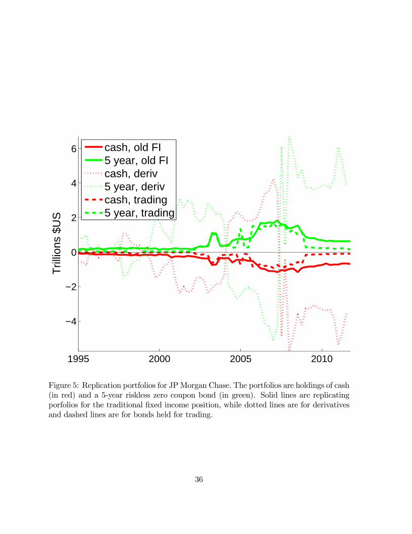
1995 2000 2005 2010

−4

−2

0

2

4

6

Tril

lions

$U

S

cash, old FI5 year, old FIcash, deriv5 year, derivcash, trading5 year, trading

Figure 5: Replication portfolios for JPMorgan Chase. The portfolios are holdings of cash

(in red) and a 5-year riskless zero coupon bond (in green). Solid lines are replicating

porfolios for the traditional fixed income position, while dotted lines are for derivatives

and dashed lines are for bonds held for trading.

36

1995 2000 2005 2010−5

0

5

Tril

lions

$U

S

JPMORGAN CHASE & CO.

cash5 year

1995 2000 2005 2010

−1

0

1

Tril

lions

$U

S

WELLS FARGO & COMPANY

1995 2000 2005 2010−4

−2

0

2

4

Tril

lions

$U

S

BANK OF AMERICA CORPORATION

2000 2005 2010

−2

−1

0

1

2

Tril

lions

$U

S

CITIGROUP INC.

Figure 6: Replication portfolios of four top dealer banks. The portfolios are holdings of

cash (in red) and a 5-year riskless zero coupon bond (in green). Solid lines are replicating

porfolios for the traditional fixed income position, while dotted lines are for derivatives

and dashed lines are for bonds held for trading.

37

References

Acharya, Viral, Pedersen, Lasse, Thomas Phillipon, and Matt Richardson 2010. “Mea-

suring Systemic Risk.” Working Paper, NYU.

Acharya, Viral, Matt Richardson, Stijn van Nieuwerburgh, and L. White 2011. “Guar-

anteed to Fail: Freddie, Fennie, and the Debacle of U.S. Mortgage Finance.” Prince-

ton University Press.

Adrian, Tobias and Hyun Song Shin 2011. “Procyclical Leverage and Value at Risk.”

Working Paper, Princeton.

Allen, Franklin 2001. “Do Financial Institutions Matter?” Journal of Finance, 56, pp.

1165-1175.

Ang, Andrew and Monika Piazzesi 2003. “A No-Arbitrage Vector Regression of Term

Structure Dynamics with Macroeconomic and Latent Variables.” Journal of Mon-

etary Economics, 50, pp. 745-787.

Brunnermeier, Markus, Gary Gorton, and Arvind Krishnamurthy 2012. “Risk Topog-

raphy.” NBER Macro Annual 2011.

Chernenko, Sergey and Faulkender, Michael 2011. “The Two Sides of Derivatives

Usage: Hedging and Speculating with Interest Rate Swaps.” Journal of Financial

and Quantitative Analysis (46), pp. 1727-1754.

Duffie, Darrell 2012. “Systemic Risk Exposures: A 10-by-10-by-10 Approach.” Systemic

Risk and Macro Modeling, Markus Brunnermeier and Arvind Krishnamurthy, ed-

itors.

Duffie, Darrell and Kenneth Singleton 1999. “Modeling Term Structures of Defaultable

Bonds.” Review of Financial Studies 12, pp. 687-720.

English, William B., Skander J. Van den Heuvel, and Egon Zakrajsek 2012. “Interest

Rate Risk and Bank Equity Valuations.” Working Paper, Federal Reserve Board.

Gorton, Gary and Richard Rosen 1995. "Banks and Derivatives". NBER Macroannual

1995, pp. 299-349.

Flannery, Mark J. and Christopher M. James 1984a. “The Effect of Interest Rate

Changes on the Common Stock Returns of Financial Institutions.” Journal of

Finance 39, 4, pp. 1141-1153.

38

Flannery, Mark J. and Christopher M. James 1984b. “Market Evidence on the Effective

Maturity of Bank Assets and Liabilities.” Journal of Money, Credit and Banking,

16, pp. 435-445.

Flannery, Mark J., Allaudeen Hammed and Richard H. Haries 1997. “Asset Pricing,

time-varying risk premia and interest rate risk.” Journal of Banking and Finance

21, pp. 315-335.

He, Zhiguo, In Gu Khang, and Arvind Krishnamurthy 2010. “Balance-Sheet Adjust-

ments during the 2008 Crisis.” IMF Economic Review 1, 118-156.

Hentschel, Ludger and S.P. Kothari 2001. “Are Corporations Reducing or Taking Risks

with Derivatives?” Journal of Financial and Quantitative Analysis 36, pp. 93-118.

Hirtle, Beverly J. 1997. “Derivatives, Portfolio Composition, and Bank Holding Com-

pany Interest Rate Risk Exposure.” Journal of Financial Services Research 12,

pp. 243-266.

Jarrow, Robert, Haitao Li, Sheen Liu, and Chunchi Wu 2010. “Reduced-form val-

uation of callable corporate bonds: Theory and Evidence.” Journal of Financial

Economics 95, pp. 227-248.

Jermann, Urban and Vivian Y. Yue 2012. “Interest Rate Swaps and Corporate De-

fault.” Working Paper, Wharton.

Kelly, Bryan, Hanno Lustig and Stijn van Nieuwerburgh 2011. “Too-Systemic-To-Fail:

What Option Markets Imply About Sector-wide Government Guarantees.” NBER

Working Paper 17149.

Landier, Augustin, David Sraer, and David Thesmar 2013. “Banks Exposure to Interest

Rate Risk and the Transmission of Monetary Policy.”NBERWorking Paper 18857.

Lustig, Hanno, Chris Sleet and Sevin Yeltekin 2008. “Fiscal hedging with nominal

assets.” Journal of Monetary Economics 55, pp. 710-727.

Minton, Bernadette, Rene Stulz and Rohan Williamson 2009. “How Much Do Banks

use Credit Derivatives to Hedge Loans?” Journal of Financial Services Research

2009, 35, pp. 1-31.

Piazzesi, Monika and Martin Schneider 2010. “Interest Rate Risk in Credit Markets”.

American Economic Review 100 (2), pp. 579-584.

Venkatachalam, Mohan 1996. “Value-relevance of banks’ derivatives disclosures.” Jour-

nal of Accounting and Economics 22, pp. 327-355.

39

Appendix

A Balance Sheet Details

This appendix provides more details about the balance sheet in Table 1. Table A.1 shows

a bank balance sheet which is based on the Consolidated Financial Statements for Bank

Holding Companies (FR-Y-9C) from December 31, 2011. These financial statements are

required by law and are filed by Bank holding companies to the Board of Governors

of the Federal Reserve System. The assets of banks include cash which can be interest

bearing (IB) or noninterest bearing (NIB) in domestic offices (DO) and foreign offices

(FO), securities, Flow of Funds sold (FFS), loans and leases, trading assets, premises and

fixed assets, other investment, intangible assets and other assets. The liabilities include

deposits, Federal Funds purchased (FFB), trading liabilities, other borrowed money,

subordinated notes, and other liabilities. The difference between assets and liabilities

is capital. The item numbers "BH" followed by more letters and numbers refer to the

entry into the financial statements by each bank holding company.

Figure 7 shows the Schedule HC-B for Securities entry in the balance sheet of Tables

1 and A.1. The schedule illustrates the asset detail available for each bank.

40

Table A.1: Bank Balance Sheets in Call Reports

Assets Liabilities

1. Cash 13. Deposits

NIB balances, currency and coin BHCK0081 a. In DO: (1) NIB BHDM6631

IB balances in US offices BHCK0395 (2) IB BHDM6636

IB balances in FO BHCK0397 b. In FO, Edges, IBFs: (1) NIB BHFN6631

(2) IB BHFN6636

2. Securities 14. FFP

a. Held-to-maturity securities BHCK1754 a. FFP in DO BHDMB993

b. Available-for-sale securities BHCK1773 b. Securities Sold to Repurchase BHCKB995

3. FFS 15. Trading Liabilities

a. FFS in DO BHDMB987 BHCK3548

b. Securities Purchased BHCKB989

4. Loans & Leases 16. Other Borrowed Money

a. Loans & leases held for sale BHCK5369 Includes mortgage, indebtness, BHCK3548

d. Loans & leases, net of unearned BHCKB529 and obligations under capitalized leases

income and allowance for (items 17., 18. are not applicable)

loan & lease losses

5. Trading Assets 19. Subordinated Notes

BHCK3545 Subordinated notes and debentures BHCK4062

Subordinated notes payable to trusts BHCKC699

6. Premises and fixed Assets 20. Other Liabilities

BHCK2145 BHCK2750

Other Investment 21. Total Liabilities

7. Other real estate owned BHCK2150 BHCK2948

8. Investments in uncons. subsidiaries BHCK2130

9. Direct & indirect investments BHCK3656

in real estate ventures

10. Intangible assets Equity

a. Goodwill BHCK3163 Total Equity Capital BHCKG105

b. Other intangible assets BHCK0426

11. Other Assets

BHCK2160

12. Total Assets BHCK2170

Abbreviations: domestic office (DO), foreign office (FO), interest baring (IB),

noninterest baring (NIB), Federal Funds sold (FFS), and Federal Funds pur-

chased (FFB).

41

Figure 7: HB-C Schedule for Securities.

42