Bar Elements in 2-D Space

By

S. Ziaei Rad

Distributed Load

=

Uniformly distributed axial load q (N/mm, N/m, lb/in) can

be converted to two equivalent nodal forces of magnitude qL/2.

We verify this by considering the work done by the load q,

Distributed Load

that is, where

Thus, from the U=W concept for the element, we have

Distributed Load

The new nodal force vector is

In an assembly of bars,

=

Bar Elements in 2-D

Note: Lateral displacement

does not contribute to the

stretch of the bar, within the

linear theory.

Transformation

In matrix form,

or, where the transformation matrix

is orthogonal, that is,

Transformation

For the two nodes of the bar element, we have

or,

The nodal forces are transformed in the same way,

Stiffness Matrix in the 2-D

SpaceIn the local coordinate system, we have

Augmenting this equation, we write

or

,

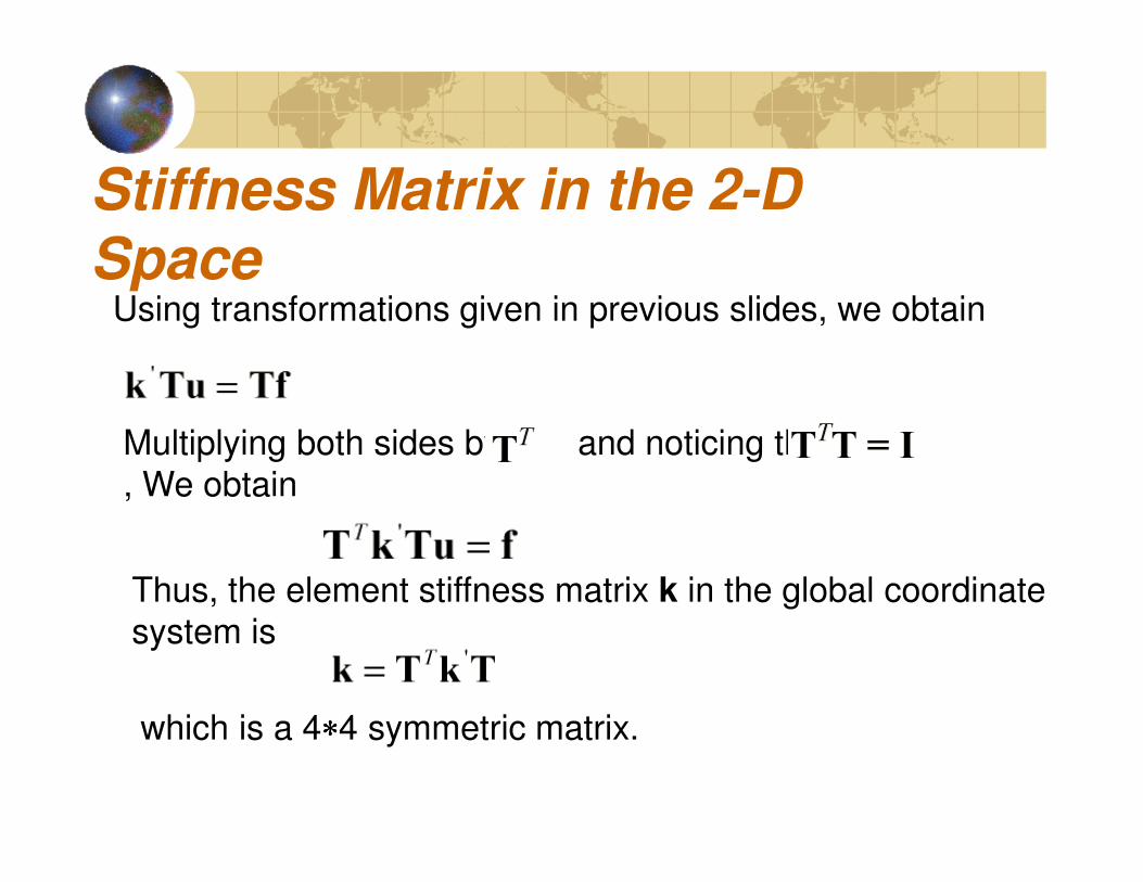
Stiffness Matrix in the 2-D

SpaceUsing transformations given in previous slides, we obtain

Multiplying both sides by and noticing that

, We obtain

Thus, the element stiffness matrix k in the global coordinate

system is

which is a 4∗∗∗∗4 symmetric matrix.

(*)

Stiffness Matrix in the 2-D

SpaceExplicit form

Calculation of the directional cosines l and m:

Note:The structure stiffness

matrix is assembled by

using the Element stiffness

matrices in the usual way a

in the 1-D case.

Assembly Rules

1. Compatibility: The joint displacements of all

members meeting at a joint must be the same.

2. Equilibrium: The sum of forces exerted by all

members that meet at a joint must balance the

external force applied to that joint.

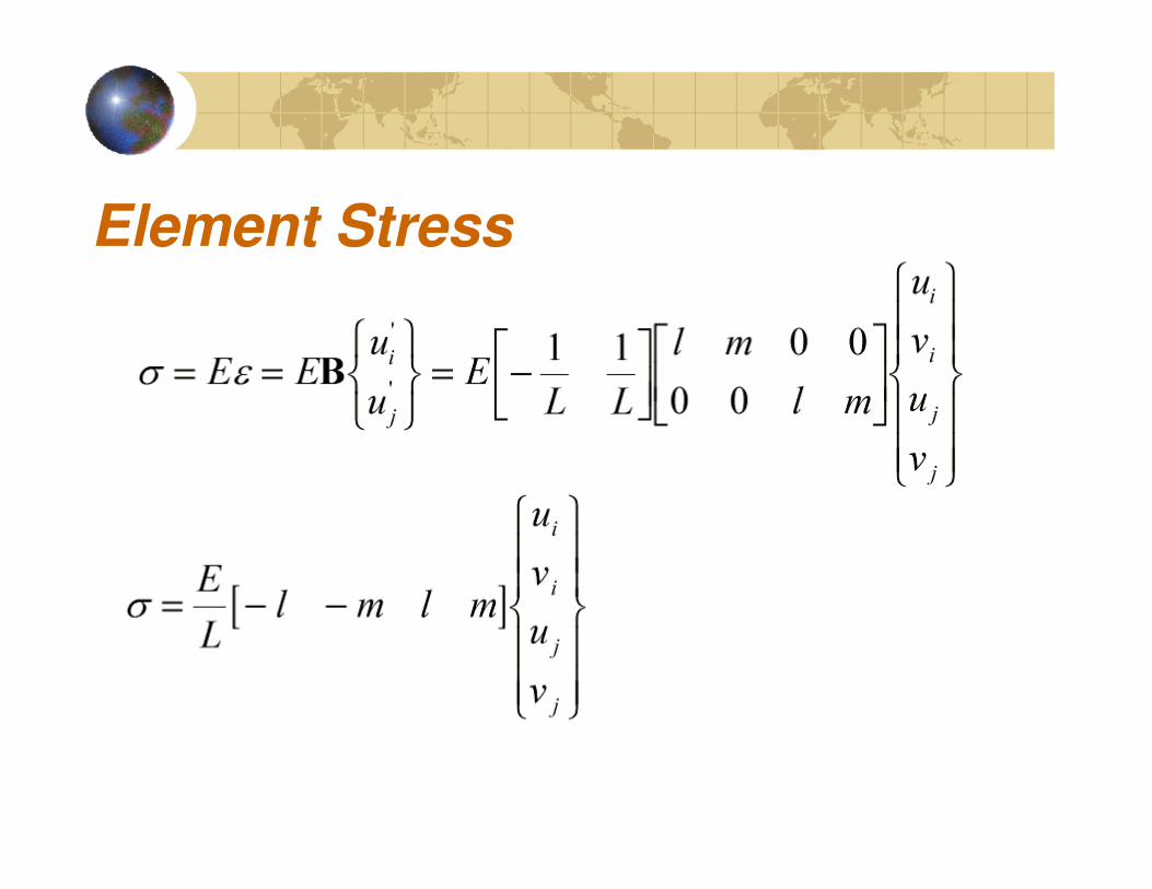
Element Stress

The Direct Stiffness Method (DSM)

Steps

Example 2.3

Problem: A simple plane truss is made

of two identical bars (with E, A, and L),

and loaded as shown in the figure. Find

1) displacement of node 2;

2) stress in each bar.

Example 2.3 (Member formation)

In local coordinate systems, we have

These two matrices cannot be assembled together, because they

are in different coordinate systems. We need to convert them to

global coordinate system OXY.

Solution: This simple structure is used here to

demonstrate the assembly and solution process using

the bar element in 2-D space.

Example 2.3 (Globalization)

Element 1:

Using formula (*), we obtain the stiffness matrix in the

global system

Example 2.3 (Globalization)

Element 2:

Using formula (*), we obtain the stiffness matrix in the

global system

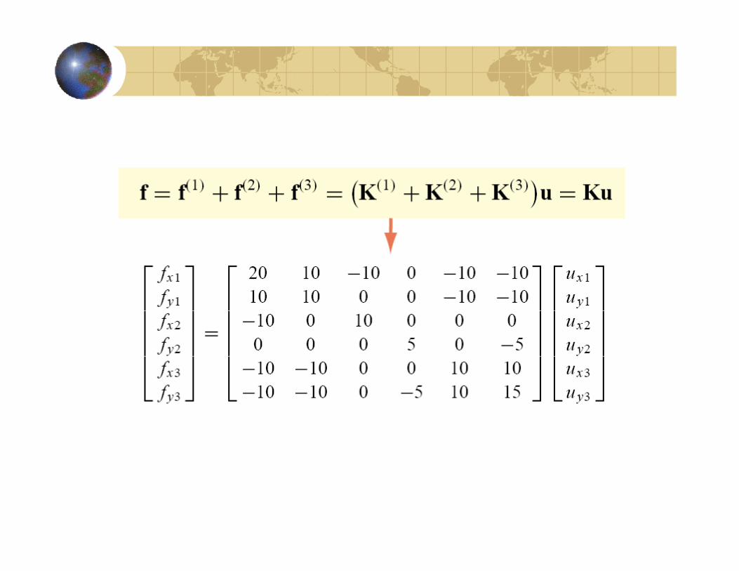
Example 2.3 (Merge or Assembly)

Assemble the structure FE equation,

Example 2.3 (Application of BCs and

Solution)Load and boundary conditions (BC):

Condensed FE equation,

Solving this, we obtain the displacement of node 2,

Example 2.3 (Recovery)

Using formula for stress, we calculate the stresses in the two bars

Example 2.4

Problem: For the plane truss shown ,

Determine the displacements and

reaction forces.

Solution: We have an inclined roller

at node 3, which needs special attention in the FE solution.

We first assemble the global FE equation for the truss.

Example 2.4Element 1:

Example 2.4

Element 2:

Example 2.4Element 3:

Example 2.4The global FE equation is,

Example 2.4Load and boundary conditions (BC):

From the transformation relation and the BC, we have

that is, This is a multipoint constraint (MPC).

Example 2.4

Similarly, we have a relation for the force at node 3,

that is,

Example 2.4Applying the load and BC’s in the structure FE equation

by ‘deleting’1st , 2nd and 4th rows and columns, we have

Further, from the MPC and the force relation at node 3, the

equation becomes,

Example 2.4

which is

The 3rd equation yields,

Substituting this into the 2nd equation and rearranging, we have

Example 2.4

Solving this, we obtain the displacements,

From the global FE equation, we can calculate the reaction

forces,

Example 2.4

A general multipoint constraint (MPC) can be described as,

where are constants and are nodal

displacement

components. In the FE software, such as ANSYS or

MSC/NASTRAN, users only need to specify this relation

to the software. The software will take care of the

solution.

THERMOMECHANICAL EFFECTS

The assumptions up to now based on the idea that truss elements

result in zero external forces under zero displacements. This is

implicit in the linear-homogeneous expression of the master stiffness

equation f = Ku.

If u vanishes, so does f. This behavior does not apply, however,

if there are initial force effects.

If those effects are present, there can be displacements without

external forces, and internal forces without displacements.

THERMOMECHANICAL EFFECTS

A common source of initial force effects are temperature changes.

Imagine that a plane truss structure is unloaded (that is, not

subjected to external forces) and is held at a uniform reference

temperature. External displacements are measured from this

environment, which is technically called a reference state. Now

suppose that the temperature of some members changes with respect

to the reference temperature while the applied external forces

remain zero. Because the length of members changes on account of

thermal expansion or contraction, the joints will displace.

Initial Force Effects (also called Initial

Strain

& Initial Stress Effects by FEM authors)

� Thermomechanical effects

� Moisture effects

� Prestress effects

� Lack of fit

� Residual stresses

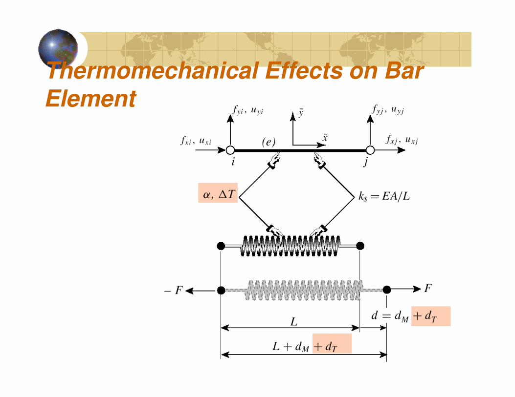
Thermomechanical Effects on Bar Element

Thermomechanical Effects on Bar

ElementAxial strain is sum of mechanical and thermal:

Incorporating Thermomechanical Effects into the Element Stiffness Equations

Generalization: Initial Force Effects

Where does come from? Thermal effects, moisture,

prestress, lack of fit, residual stresses, some nonlinearities.

Common property: if displacements u vanish

IMIM ffff −=⇒=+ 0

There are (self-equilibrating) mechanical forces in the

absence of displacements

Suppose that the example truss is now unloaded. However the

temperature of members (1) (2) and (3) changes by T ,−T and 3T ,

respectively, with respect to Tref .

The thermal expansion coefficient of all three members is assumed

to be α.

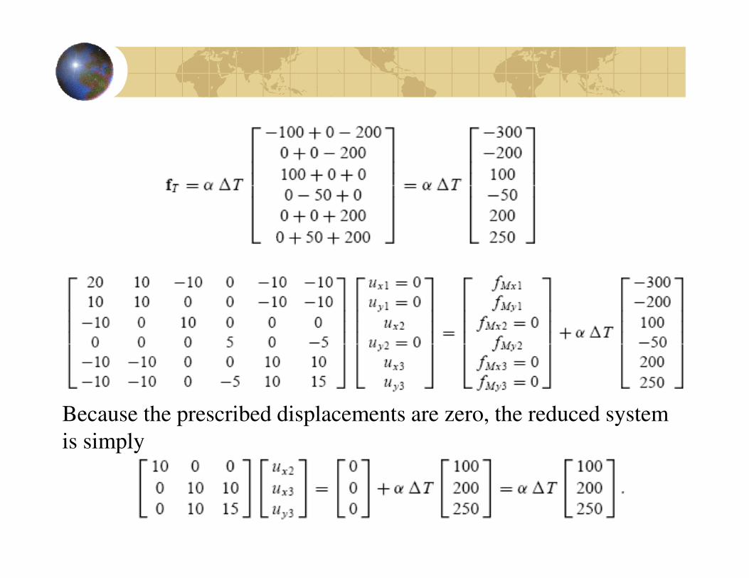
Because the prescribed displacements are zero, the reduced system

is simply

Solving

Treating Initial Force Effects

How to Write a Simple MATLAB Program for 2D bar

PreprocessorNodes, Elements ,Members Properties (Geometry, Material)

Element Stiffness Matrices(Local Coordinates)

Element Stiffness Matrices(Global Coordinates)

Forming Global Stiffness Matrix and Force Vector

Apply the B.C.

Solution Phase

Postprocessing

A MATLAB Program

Clear

Node=[

node_no1 x1 y1

node_no2 x2 y2

………………];

Element=[

elem_no node_no1 node_no2 length theta E A

………………];

BCdof=[…………………];

F_global=[ fx1 fy1 fx2 fy2 …………………]’;

Connectivity=[

elem_no Dof1 Dof2 Dof3 Dof4

………………];

(NN,MN)=size(Node) ;

(NE,ME=size(Element);

K_global=zeros(NN*2,NN*2);

A MATLAB Program

for i=1:NE

Ke_local=Kelocal (Element(i,4), Element(i,6), Element(i,7)); % Kelocal is a Matlab function

Te_rotatoin=T_rotation(Element(i,5)); % T_rotation is a Matlab function

Ke_global==Te_rotation'*ke_local*Te_rotation;

ke_assemble=Assemble(Ke_global,Connectivity(i,:),NN); % Assemble is a Matlab function

K_global= K_global+ke_assemble

end

% F_global=[ fx1 fy1 fx2 fy2 …………………]’;

% Assume that the external forces are in global coordinates

% If they are in local coordinates then they have to transfer using

% F_global=Te_rotation*Fe_local

% Applying the B.C

K_globalBC=Boundry_conditionK(K_global,BCdof)

F_globalBC=Boundry_conditionF(F_global, BCdof)

% Solution Phase

U=inv(K_globalBC)*F_globalBC;

A MATLAB Program

% Postprocessing Phase

for i=1:NE

stress(i)=Stress_calc(U, Element(i,2), Element(i,3),Element(i,4), Element(i,5) );

end

% end of the program

end