Basic Statistics and Shannon Entropy

Ka-Lok Ng

Asia University

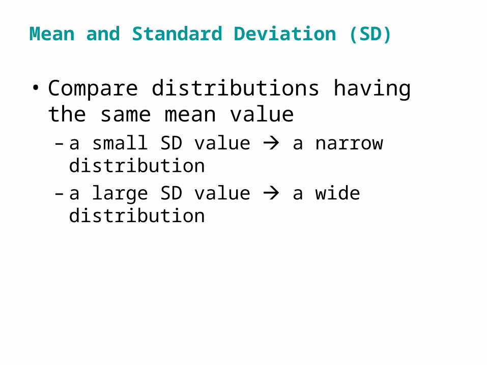
Mean and Standard Deviation (SD)

• Compare distributions having the same mean value– a small SD value a narrow distribution– a large SD value a wide distribution

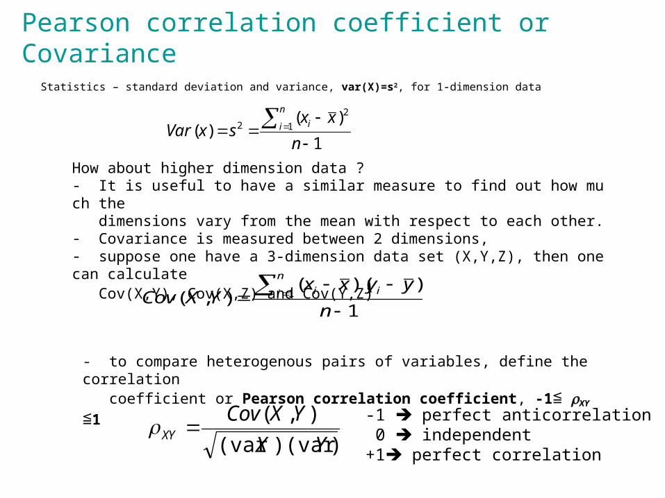
Pearson correlation coefficient or Covariance

Statistics – standard deviation and variance, var(X)=s2, for 1-dimension data

How about higher dimension data ? - It is useful to have a similar measure to find out how much the dimensions vary from the mean with respect to each other. - Covariance is measured between 2 dimensions,- suppose one have a 3-dimension data set (X,Y,Z), then one can calculate Cov(X,Y), Cov(X,Z) and Cov(Y,Z)

- to compare heterogenous pairs of variables, define the correlation coefficient or Pearson correlation coefficient, -1≦ XY ≦1

))(var(var

),(

YX

YXCovXY -1 perfect anticorrelation

0 independent+1 perfect correlation

1

)()( 1

22

n

xxsxVar

n

i i

1

))((),( 1

n

yyxxYXCov

n

i ii

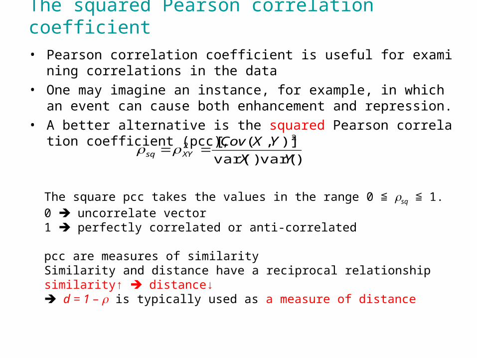
The squared Pearson correlation coefficient

• Pearson correlation coefficient is useful for examining correlations in the data

• One may imagine an instance, for example, in which an event can cause both enhancement and repression.

• A better alternative is the squared Pearson correlation coefficient (pcc),

)var()var(

)],([ 22

YX

YXCovXYsq

The square pcc takes the values in the range 0 ≦ sq 1.≦0 uncorrelate vector1 perfectly correlated or anti-correlated

pcc are measures of similaritySimilarity and distance have a reciprocal relationshipsimilarity↑ distance↓ d = 1 – is typically used as a measure of distance

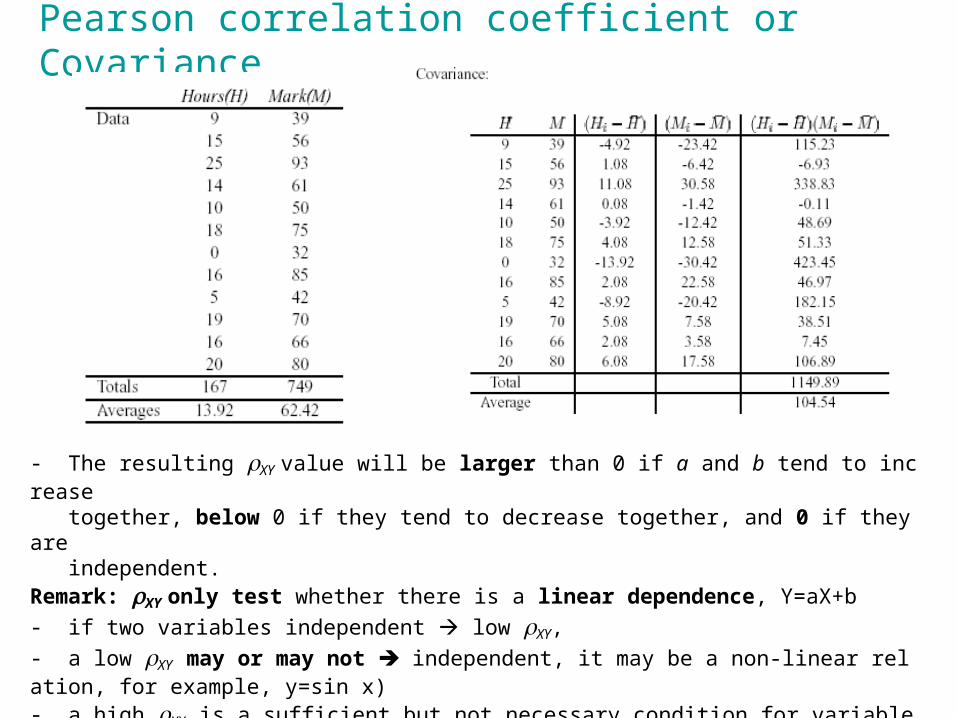
Pearson correlation coefficient or Covariance

- The resulting XY value will be larger than 0 if a and b tend to increase together, below 0 if they tend to decrease together, and 0 if they are independent.Remark: XY only test whether there is a linear dependence, Y=aX+b- if two variables independent low XY, - a low XY may or may not independent, it may be a non-linear relation, for example, y=sin x)- a high XY is a sufficient but not necessary condition for variable dependence

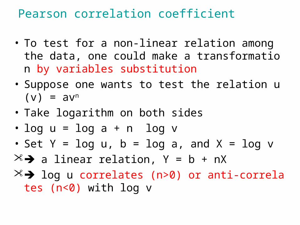
Pearson correlation coefficient

• To test for a non-linear relation among the data, one could make a transformation by variables substitution

• Suppose one wants to test the relation u(v) = avn

• Take logarithm on both sides• log u = log a + n log v • Set Y = log u, b = log a, and X = log v a linear relation, Y = b + nX log u correlates (n>0) or anti-correlates (n<0) w

ith log v

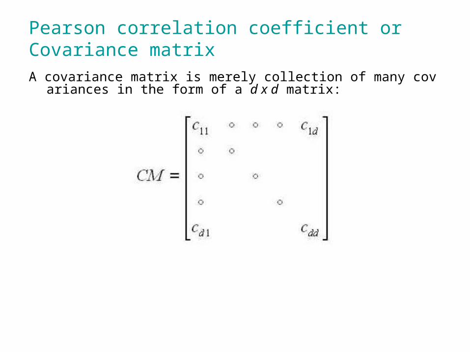
Pearson correlation coefficient or Covariance matrixA covariance matrix is merely collection of many covariances in the for

m of a d x d matrix:

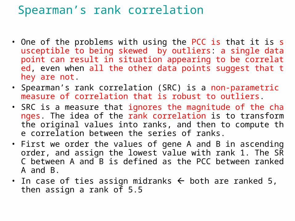
Spearman’s rank correlation

• One of the problems with using the PCC is that it is susceptible to being skewed by outliers: a single data point can result in situation appearing to be correlated, even when all the other data points suggest that they are not.

• Spearman’s rank correlation (SRC) is a non-parametric measure of correlation that is robust to outliers.

• SRC is a measure that ignores the magnitude of the changes. The idea of the rank correlation is to transform the original values into ranks, and then to compute the correlation between the series of ranks.

• First we order the values of gene A and B in ascending order, and assign the lowest value with rank 1. The SRC between A and B is defined as the PCC between ranked A and B.

• In case of ties assign midranks both are ranked 5, then assign a rank of 5.5

Spearman’s rank correlation

n

i i

n

i i

n

i iiSRC

yyxx

yyxxYX

1

2

1

2

1

])(][)([

))((),(

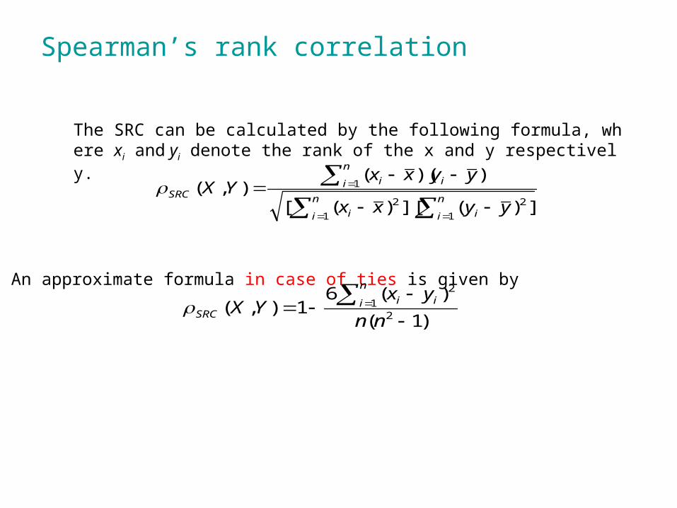
The SRC can be calculated by the following formula, where xi and yi denote the rank of the x and y respectively.

An approximate formula in case of ties is given by

)1(

)(61),(

21

2

nn

yxYX

n

i iiSRC

Distances in discretized space

• Sometimes one has to due with discreteized values

• The similarity between two discretized vectors can be measured by the notion of Shannon entropy.

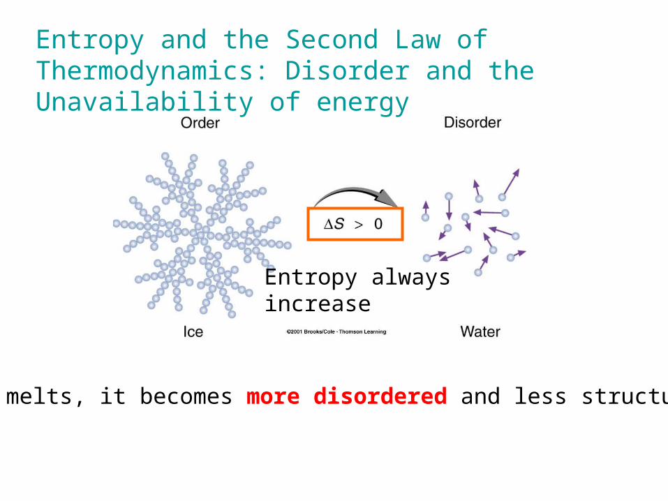
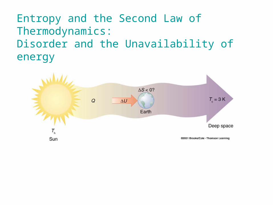
Entropy and the Second Law of Thermodynamics: Disorder and the Unavailability of energy

Ice melts, it becomes more disordered and less structured.

Entropy alwaysincrease

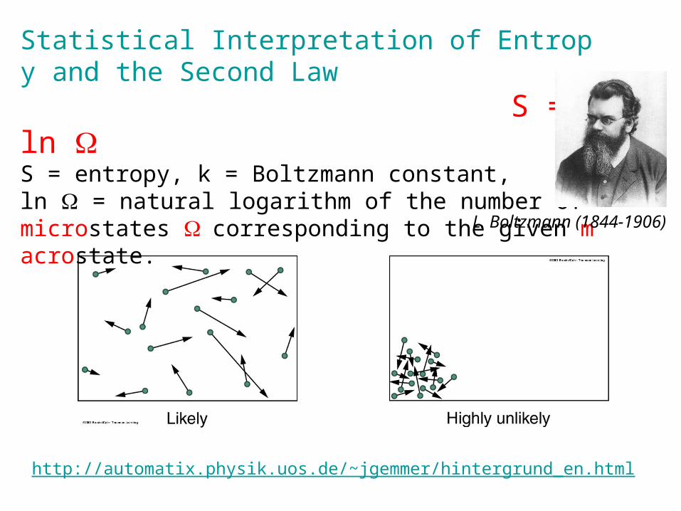
Statistical Interpretation of Entropy and the Second Law S = k ln S = entropy, k = Boltzmann constant, ln = natural logarithm of the number of microstates corresponding to the given macrostate.

L. Boltzmann (1844-1906)

http://automatix.physik.uos.de/~jgemmer/hintergrund_en.html

Entropy and the Second Law of Thermodynamics: Disorder and the Unavailability of energy

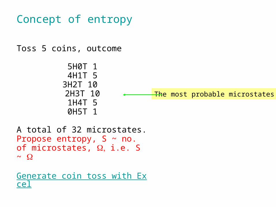
Concept of entropy

Toss 5 coins, outcome

5H0T 14H1T 5

3H2T 10 2H3T 101H4T 50H5T 1

A total of 32 microstates. Propose entropy, S ~ no. of microstates, i.e. S ~

Generate coin toss with Excel

The most probable microstates

Shannon entropy

• Shannon entropy is related to physical entropy• Shannon ask the question “What is information ?”• Energy is defined as the capacity to do work, not the work itself. Work is a fo

rm of energy.• Define information as the capacity to store and transmit meaning or knowled

ge, not the meaning or knowledge itself.• For example, a lot of information from WWW, but it does not mean knowled

ge• Shannon suggest entropy is the measure of this capacitySummary

Define information capacity to store knowlege entropy is the measure Shannon entropy

Entropy ~ randomness ~ measure of capacity to store and transmit knowledge

Reference: Gatlin L.L, Information theory and the living system, Columbia University Press, New York, 1972.

Shannon entropy

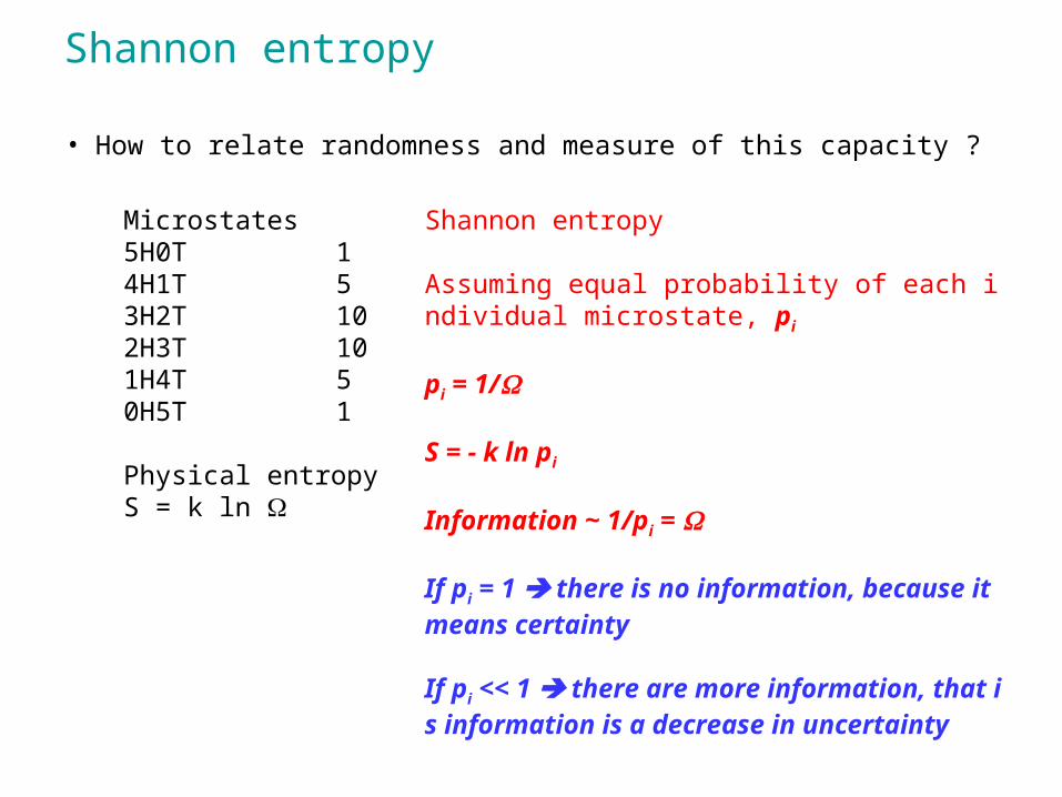
• How to relate randomness and measure of this capacity ?

Microstates5H0T 14H1T 53H2T 10 2H3T 101H4T 50H5T 1

Physical entropyS = k ln

Shannon entropy

Assuming equal probability of each individual microstate, pi

pi = 1/

S = - k ln pi

Information ~ 1/pi =

If pi = 1 there is no information, because it means certainty

If pi << 1 there are more information, that is information is a decrease in uncertainty

Distances in discretized space

n

i ii ppH11 log

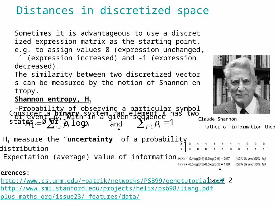
Sometimes it is advantageous to use a discretized expression matrix as the starting point, e.g. to assign values 0 (expression unchanged, 1 (expression increased) and -1 (expression decreased).The similarity between two discretized vectors can be measured by the notion of Shannon entropy.Shannon entropy, H1

-Probability of observing a particular symbol or event, pi, with in a given sequence

Consider a binary system, an element X has two states, 0 or 1

base 2References: 1. http://www.cs.unm.edu/~patrik/networks/PSB99/genetutorial.pdf2. http://www.smi.stanford.edu/projects/helix/psb98/liang.pdf3. plus.maths.org/issue23/ features/data/

Claude Shannon

- father of information theory

- H1 measure the “uncertainty” of a probability distribution- Expectation (average) value of information

11

n

i ipand

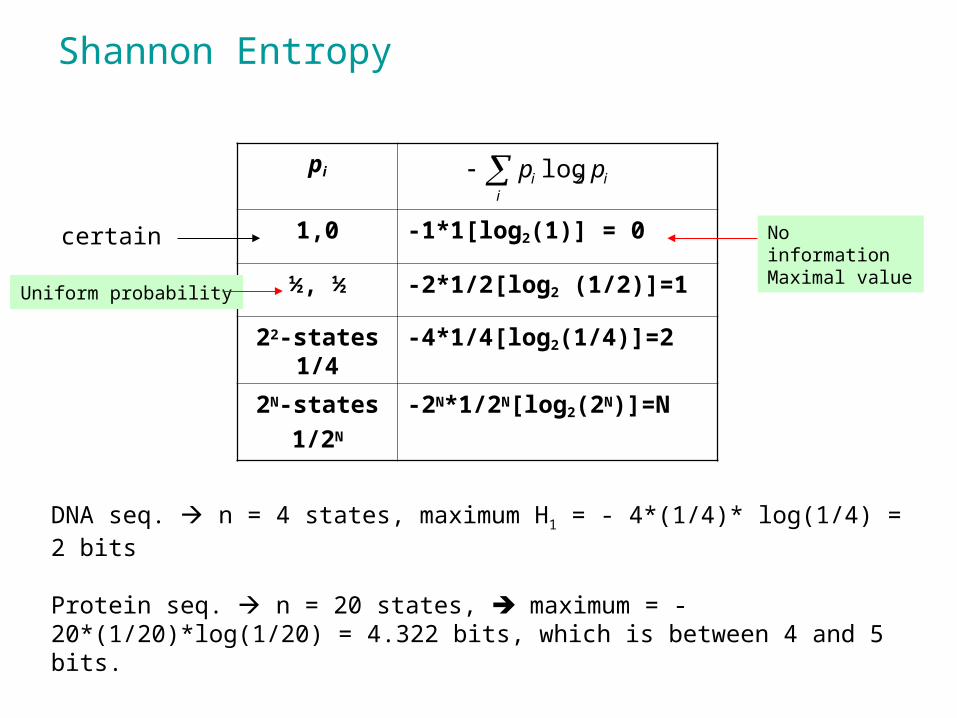
Shannon Entropy

pi

1,0 -1*1[log2(1)] = 0

½, ½ -2*1/2[log2 (1/2)]=1

22-states 1/4 -4*1/4[log2(1/4)]=2

2N-states

1/2N

-2N*1/2N[log2(2N)]=N

ii

i pp 2log

Uniform probability

certain No informationMaximal value

DNA seq. n = 4 states, maximum H1 = - 4*(1/4)* log(1/4) = 2 bits

Protein seq. n = 20 states, maximum = - 20*(1/20)*log(1/20) = 4.322 bits, which is between 4 and 5 bits.

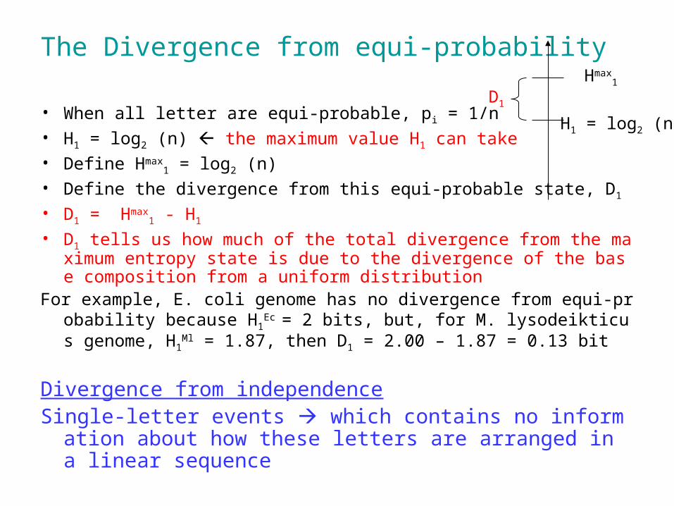
The Divergence from equi-probability

• When all letter are equi-probable, pi = 1/n• H1 = log2 (n) the maximum value H1 can take• Define Hmax

1 = log2 (n) • Define the divergence from this equi-probable state, D1

• D1 = Hmax1 - H1

• D1 tells us how much of the total divergence from the maximum entropy state is due to the divergence of the base composition from a uniform distribution

For example, E. coli genome has no divergence from equi-probability because H1

Ec = 2 bits, but, for M. lysodeikticus genome, H1

Ml = 1.87, then D1 = 2.00 – 1.87 = 0.13 bit

Divergence from independenceSingle-letter events which contains no information about

how these letters are arranged in a linear sequence

Hmax1

H1 = log2 (n)

D1

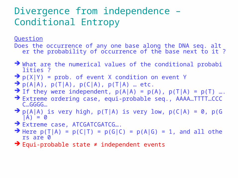
Divergence from independence – Conditional Entropy

QuestionDoes the occurrence of any one base along the DNA seq. alter the pro

bability of occurrence of the base next to it ? What are the numerical values of the conditional probabilities ? p(X|Y) = prob. of event X condition on event Y p(A|A), p(T|A), p(C|A), p(T|A) … etc. If they were independent, p(A|A) = p(A), p(T|A) = p(T) …. Extreme ordering case, equi-probable seq., AAAA…TTTT…CCCC

…GGGG… p(A|A) is very high, p(T|A) is very low, p(C|A) = 0, p(G|A) = 0 Extreme case, ATCGATCGATCG…. Here p(T|A) = p(C|T) = p(G|C) = p(A|G) = 1, and all others are 0 Equi-probable state ≠ independent events

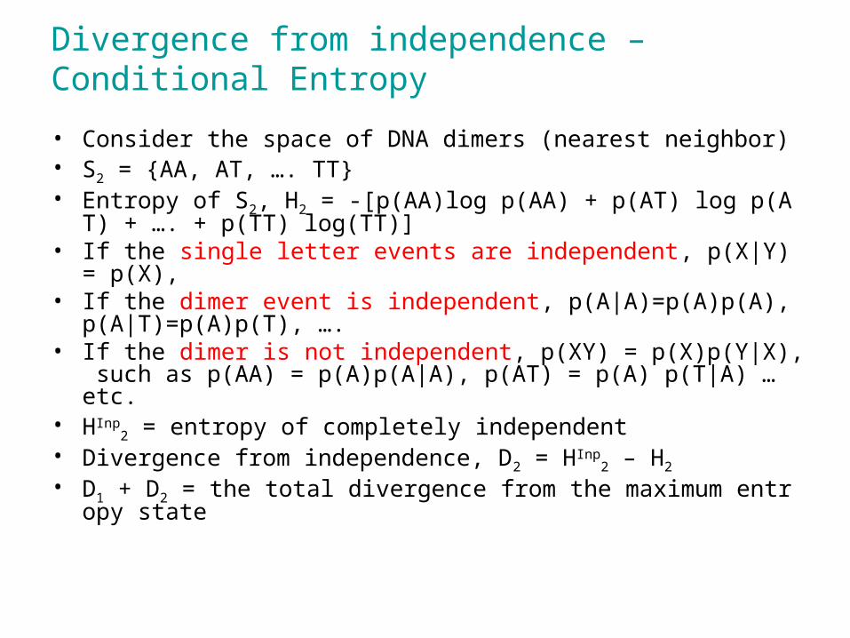
Divergence from independence – Conditional Entropy

• Consider the space of DNA dimers (nearest neighbor)• S2 = {AA, AT, …. TT}• Entropy of S2, H2 = -[p(AA)log p(AA) + p(AT) log p(AT) + …. + p(TT)

log(TT)]• If the single letter events are independent, p(X|Y) = p(X),• If the dimer event is independent, p(A|A)=p(A)p(A), p(A|T)=p(A)p(T),

…. • If the dimer is not independent, p(XY) = p(X)p(Y|X), such as p(AA) =

p(A)p(A|A), p(AT) = p(A) p(T|A) … etc.• HInp

2 = entropy of completely independent• Divergence from independence, D2 = HInp

2 – H2

• D1 + D2 = the total divergence from the maximum entropy state

Divergence from independence – Conditional Entropy

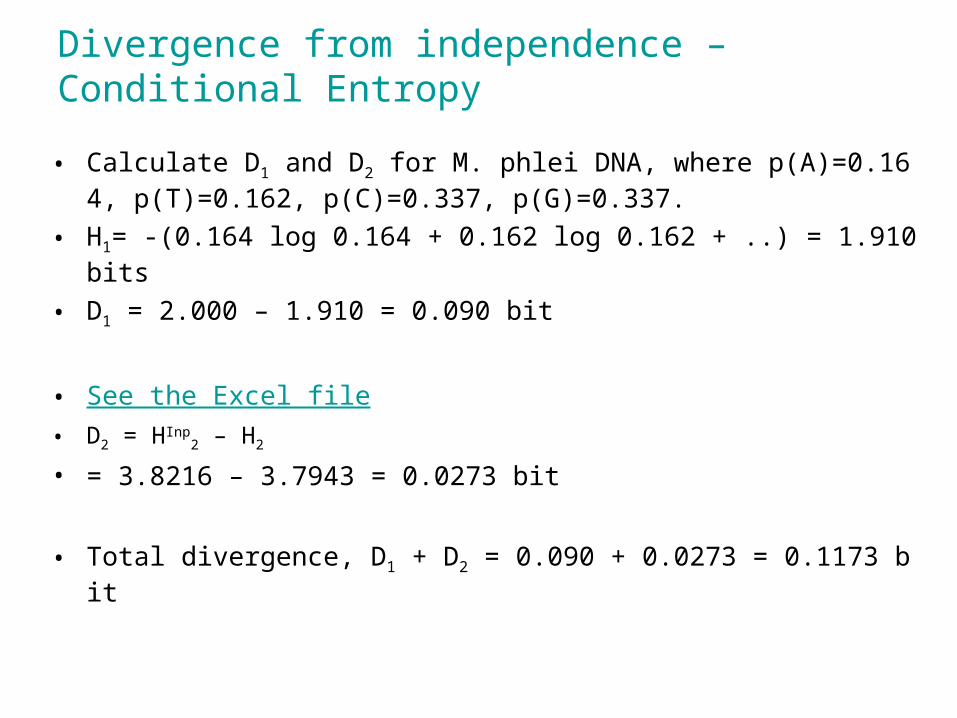
• Calculate D1 and D2 for M. phlei DNA, where p(A)=0.164, p(T)=0.162, p(C)=0.337, p(G)=0.337.

• H1= -(0.164 log 0.164 + 0.162 log 0.162 + ..) = 1.910 bits

• D1 = 2.000 – 1.910 = 0.090 bit

• See the Excel file• D2 = HInp

2 – H2

• = 3.8216 – 3.7943 = 0.0273 bit

• Total divergence, D1 + D2 = 0.090 + 0.0273 = 0.1173 bit

Divergence from independence – Conditional Entropy

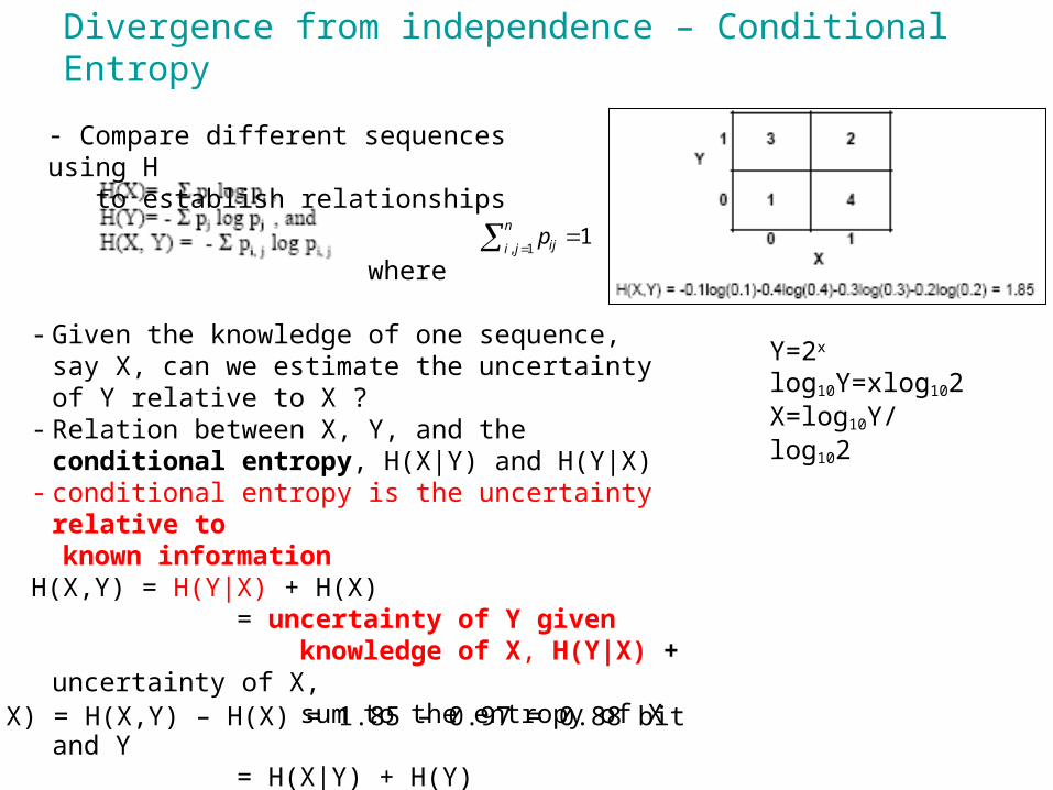
- Compare different sequences using H to establish relationships

- Given the knowledge of one sequence, say X, can we estimate the uncertainty of Y relative to X ?

- Relation between X, Y, and the conditional entropy, H(X|Y) and H(Y|X)

- conditional entropy is the uncertainty relative to known informationH(X,Y) = H(Y|X) + H(X) = uncertainty of Y given knowledge of X, H(Y|X) + uncertainty of X, sum to the entropy of X and Y = H(X|Y) + H(Y)

Y=2x

log10Y=xlog102X=log10Y/log102

H(Y|X) = H(X,Y) – H(X) = 1.85 – 0.97 = 0.88 bit

11,

n

ji ijp

where

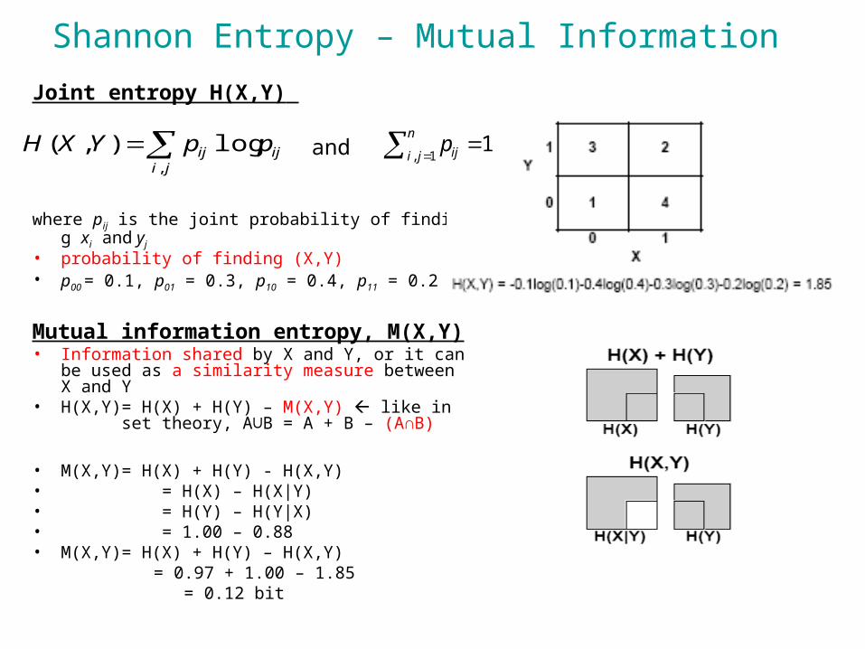
Shannon Entropy – Mutual Information

Joint entropy H(X,Y)

where pij is the joint probability of finding xi and yj

• probability of finding (X,Y) • p00 = 0.1, p01 = 0.3, p10 = 0.4, p11 = 0.2

Mutual information entropy, M(X,Y)• Information shared by X and Y, or it can be us

ed as a similarity measure between X and Y• H(X,Y)= H(X) + H(Y) – M(X,Y) like in se

t theory, A B = A + B – ∪ (A∩B)

• M(X,Y)= H(X) + H(Y) - H(X,Y) • = H(X) – H(X|Y)• = H(Y) – H(Y|X)• = 1.00 – 0.88• M(X,Y)= H(X) + H(Y) – H(X,Y) = 0.97 + 1.00 – 1.85 = 0.12 bit

ji

ijij ppYXH,

log),( 11,

n

ji ijpand

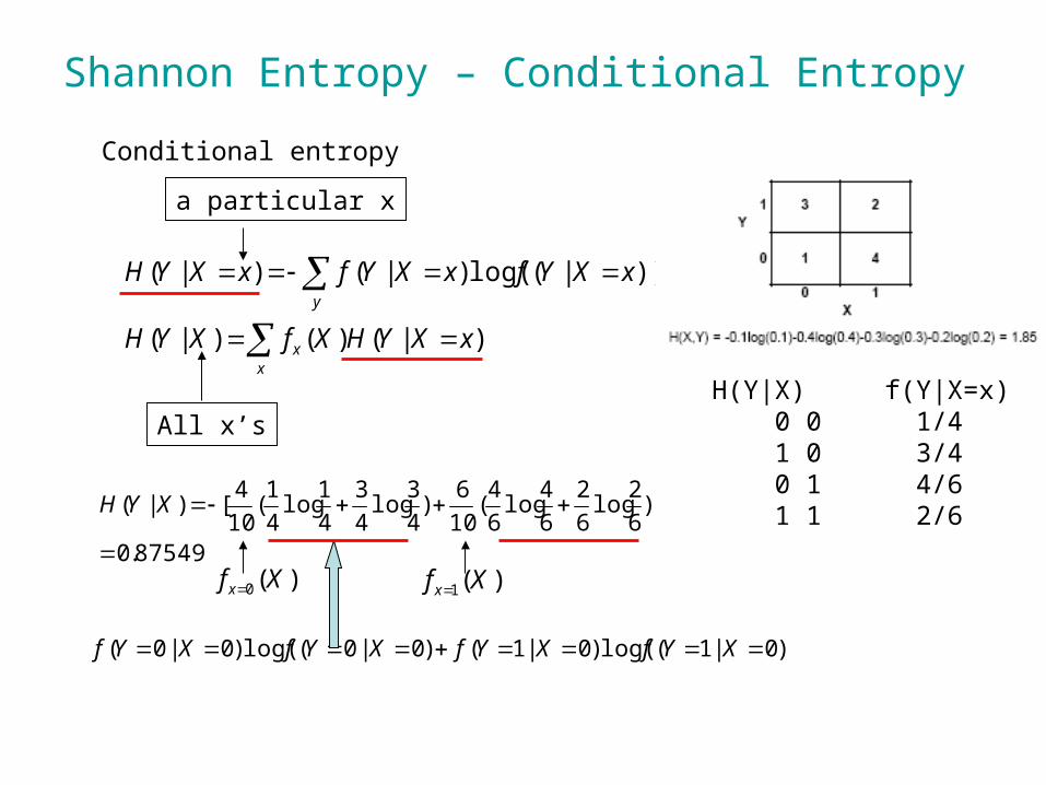
Shannon Entropy – Conditional Entropy

)(0 Xf x

)0|1(log()0|1()0|0(log()0|0( XYfXYfXYfXYf

)|()()|(

))|(log()|()|(

xXYHXfXYH

xXYfxXYfxXYH

xx

y

87549.0

)]6

2log

6

2

6

4log

6

4(

10

6)

4

3log

4

3

4

1log

4

1(

10

4[)|(

XYH

H(Y|X) f(Y|X=x) 0 0 1/4 1 0 3/4 0 1 4/6 1 1 2/6

Conditional entropy

a particular x

All x’s

)(1 Xf x