Embed Size (px)
Citation preview
Bayesian Adaptive Methods forClinical Trials
Pfizer Research Technology Center, Cambridge, MA
March 2, 2012
presented by
Bradley P. Carlin
University of Minnesota
Bayesian Adaptive Methods for Clinical Trials – p. 1/100
Textbooks for this courseRecommended
(“BCLM”): Bayesian Adaptive Methods for ClinicalTrials (ISBN 978-1-4398-2548-8) by S.M. Berry, B.P.Carlin, J.J. Lee, and P. Müller, Boca Raton, FL:Chapman and Hall/CRC Press, 2010.
Other books of interest:Your favorite math stat and linear models booksBayesian Methods for Data Analysis, 3rd ed., by B.P.Carlin and T.A. Louis, Boca Raton, FL: Chapmanand Hall/CRC Press, 2009.Bayesian Approaches to Clinical Trials andHealth-Care Evaluation, by D.J. Spiegelhalter, K.R.Abrams, and J.P. Myles: Chichester: Wiley, 2004.
Bayesian Adaptive Methods for Clinical Trials – p. 4/100

Software for Bayesian CTs IExpensive but incredibly cool commercial software: FACTS(Fixed and Adaptive Clinical Trials Simulator) software formany Phase I and II trial designs
permits dose finding in the presence of both safety andefficacy endpoints; stopping for success or futility
supports continuous, dichotomous, or time-to-event(TITE) endpoints; also longitudinal data (e.g.biomarkers)
joint venture between Berry Consultants (statistics,algorithms) and Tessella Technology and Consulting(software interface)
Website:http://www.smarterclinicaltrials.com/what-we-offer/facts/– probably best for large companies with ongoingcommitments to Bayesian CT development
Bayesian Adaptive Methods for Clinical Trials – p. 38/100
Software for Bayesian CTs IINoncommercial but still very professional software: freelyavailable from the M.D. Anderson Cancer CenterDepartment of Biostatistics Software page,https://biostatistics.mdanderson.org/SoftwareDownload/
All are stand-alone packages, free for download andlocal install
easy to learn: menu- and dialog box-driven, nicegraphics where appropriate
accompanied by extensive tutorials, typically withguidelines, exercises, and solutions
remarkably broad coverage of areas from all phases ofthe regulatory process...
Bayesian Adaptive Methods for Clinical Trials – p. 39/100
Software for Bayesian CTs IIPartial list of MD Anderson Phase I software packages:
CRMSimulator: Simulates power and Type I error ofContinual Reassessment Method (CRM) dose-findingdesigns, offering improvements in power and/or samplesize over “3 + 3" designs; see BCLM Section 3.2.
bCRM: handles bivariate dose-finding with twocompeting outcomes (say, toxicity and progression) anda single agent; see BCLM Section 3.4.2.
EffTox: finds a best dose when efficacy must be tradedoff against toxicity, both assumed increasing in dose;see BCLM Section 3.3.
ToxFinder: for combination therapy, i.e., two drugsbeing administered in combination, with only oneoutcome (usually toxicity); see BCLM Section 3.4.4.
Bayesian Adaptive Methods for Clinical Trials – p. 40/100
Software for Bayesian CTs IIPartial list of MD Anderson Phase II software packages:
Phase II PP Design: computes stopping boundaries fora single-arm Phase II predictive probability design witha binary endpoint; see BCLM Section 4.2.
MultcLean: for monitoring toxicity and efficacy in singlearm phase II clinical trials with binary data; see BCLMSection 4.3.2.
Adaptive Randomization (AR): for designing andsimulating outcome-adaptive randomized trials with upto 10 arms, using binary or time-to-event (TITE)outcomes; more patients are treated with the bettertreatment while retaining the benefits of randomization;see BCLM Section 4.4.
Bayesian Adaptive Methods for Clinical Trials – p. 41/100
Software for Bayesian CTs IIINoncommercial and not-all-that-professional software, butwith R and BUGS source code freely available: from theBCLM book’s data and software page,http://www.biostat.umn.edu/∼brad/data3.html
organized by chapter in the book
similar range of models/problems as the MDACCsoftware
continuing to grow
Mostly written in R, but those that require MCMCtypically call OpenBUGS using the BRugs package,whose installation and exemplification are given here:http://www.biostat.umn.edu/∼brad/software/BRugs/
Bayesian Adaptive Methods for Clinical Trials – p. 42/100
Software for Bayesian CTs IIIPartial list of BCLM Phase I software packages:
betabinHM.R: elementary BRugs metaanalysis programfor a single success proportion; see BCLM Section 2.4.
Power_BRugs.txt: slightly more advanced BRugs powerand Type I error-simulating program, Weibull survivalmodel; see BCLM Section 2.5.4.
titecrm.R: a basic R implementation of the TITE-CRMmethod; see BCLM Section 3.2.3.
324.R: an R program for dose-finding based on toxicityintervals (rather than fixed target levels); see BCLMSection 3.2.4.
354.R: a basic R implementation of the 2-agentcombination therapy dose-escalation method (similar toToxFinder); see BCLM Section 3.4.4.
Bayesian Adaptive Methods for Clinical Trials – p. 43/100
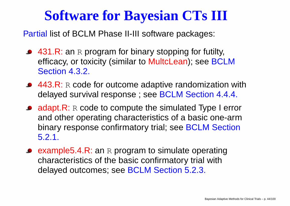
Software for Bayesian CTs IIIPartial list of BCLM Phase II-III software packages:
431.R: an R program for binary stopping for futilty,efficacy, or toxicity (similar to MultcLean); see BCLMSection 4.3.2.
443.R: R code for outcome adaptive randomization withdelayed survival response ; see BCLM Section 4.4.4.
adapt.R: R code to compute the simulated Type I errorand other operating characteristics of a basic one-armbinary response confirmatory trial; see BCLM Section5.2.1.
example5.4.R: an R program to simulate operatingcharacteristics of the basic confirmatory trial withdelayed outcomes; see BCLM Section 5.2.3.
Bayesian Adaptive Methods for Clinical Trials – p. 44/100
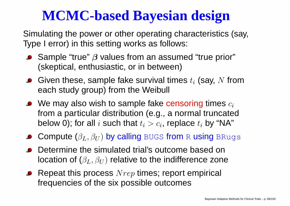
MCMC-based Bayesian designSimulating the power or other operating characteristics (say,Type I error) in this setting works as follows:
Sample “true” β values from an assumed “true prior”(skeptical, enthusiastic, or in between)
Given these, sample fake survival times ti (say, N fromeach study group) from the Weibull
We may also wish to sample fake censoring times cifrom a particular distribution (e.g., a normal truncatedbelow 0); for all i such that ti > ci, replace ti by “NA”
Compute (βL, βU ) by calling BUGS from R using BRugs
Determine the simulated trial’s outcome based onlocation of (βL, βU ) relative to the indifference zone
Repeat this process Nrep times; report empiricalfrequencies of the six possible outcomes
Bayesian Adaptive Methods for Clinical Trials – p. 68/100
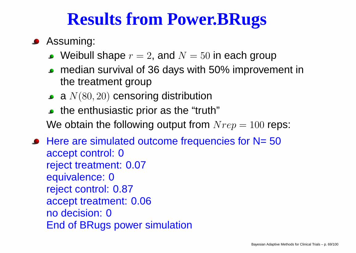
Results from Power.BRugsAssuming:
Weibull shape r = 2, and N = 50 in each groupmedian survival of 36 days with 50% improvement inthe treatment groupa N(80, 20) censoring distributionthe enthusiastic prior as the “truth”
We obtain the following output from Nrep = 100 reps:
Here are simulated outcome frequencies for N= 50accept control: 0reject treatment: 0.07equivalence: 0reject control: 0.87accept treatment: 0.06no decision: 0End of BRugs power simulation
Bayesian Adaptive Methods for Clinical Trials – p. 69/100
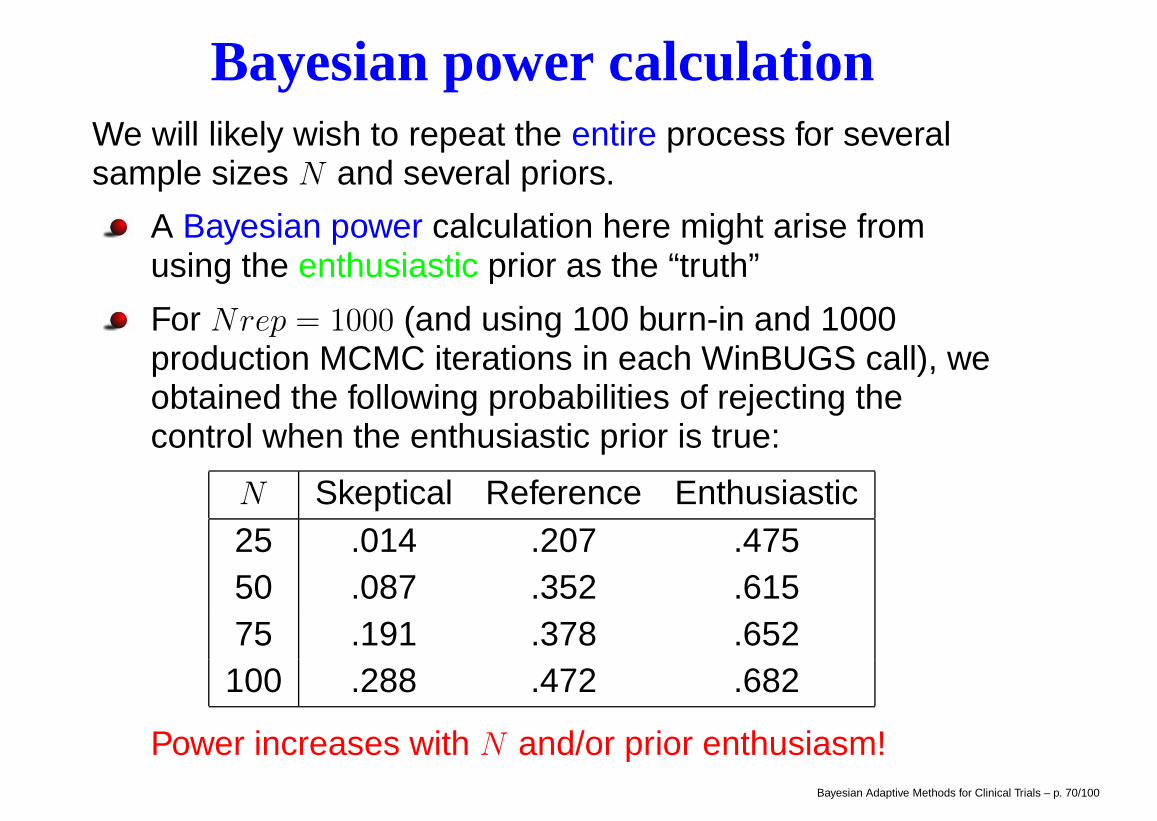
Bayesian power calculationWe will likely wish to repeat the entire process for severalsample sizes N and several priors.
A Bayesian power calculation here might arise fromusing the enthusiastic prior as the “truth”
For Nrep = 1000 (and using 100 burn-in and 1000production MCMC iterations in each WinBUGS call), weobtained the following probabilities of rejecting thecontrol when the enthusiastic prior is true:
N Skeptical Reference Enthusiastic25 .014 .207 .47550 .087 .352 .61575 .191 .378 .652100 .288 .472 .682
Power increases with N and/or prior enthusiasm!Bayesian Adaptive Methods for Clinical Trials – p. 70/100
Type I error rate calculationA Bayesian version of this calculation would arisesimilar to the method of the previous slide, but nowassuming the skeptical prior is true
A true frequentist Type I error calculation is alsopossible: simply fix β1 = 0, and generate only the ti andci for each of the Nrep iterations.
Note that while Bayesians are free to look at their dataat any time without affecting the inference, multiplelooks will alter the frequentist Type I error behavior ofthe procedure. If this is of interest, the algorithm mustbe modified to explicitly include these multiple looks,checking for early stopping after each look.
Early stopping for futility based on predictivedistributions (“Bayesian stochastic curtailment”) mayalso be of interest – see Berry and Berry (2004)!
Bayesian Adaptive Methods for Clinical Trials – p. 71/100
Ch 3: Phase I studiesThe first application of a new drug to humans
Typically small (20-50 patients)
Main goal: to establish the safety of a proposed drug,often through determining an appropriate dosingschedule (dose-finding)
For cytotoxic agents (cancer), we assume the drugbenefit (as well as the severity of its toxicity and otherside effects) increases with dose, and thus seek themaximum tolerated dose (MTD)
Key elements:
a starting dose (often 110LD10,mice)
a definition of dose limiting toxicity (DLT)a target toxicity level (TTL) (say, 20-30%)a dose escalation scheme
Bayesian Adaptive Methods for Clinical Trials – p. 72/100
Sec 3.1: Rule-based MTD designsAlter the dose based on the toxicity observed in theprevious cohort. Most common: the 3+3 design:
1. Enter 3 patients at the lowest dose level
2. Observe the toxicity outcome:if 0/3 DLT ⇒ Treat next 3 patients at next higher doseif 1/3 DLT ⇒ Treat next 3 patients at the same dose;
if 0/3 DLT ⇒ Treat next 3 at next higher doseif 1/3 ⇒ Define this dose as MTDif 2/3 or 3/3 DLT ⇒ dose exceeds MTD
if 2/3 or 3/3 DLT ⇒ dose exceeds MTD
3. Repeat Step 2. If the last dose exceeds MTD, definethe previous dose as MTD provided 6 or more patientshave been treated at that dose.
4. MTD is defined as a dose with ≤ 2/6 DLTBayesian Adaptive Methods for Clinical Trials – p. 73/100
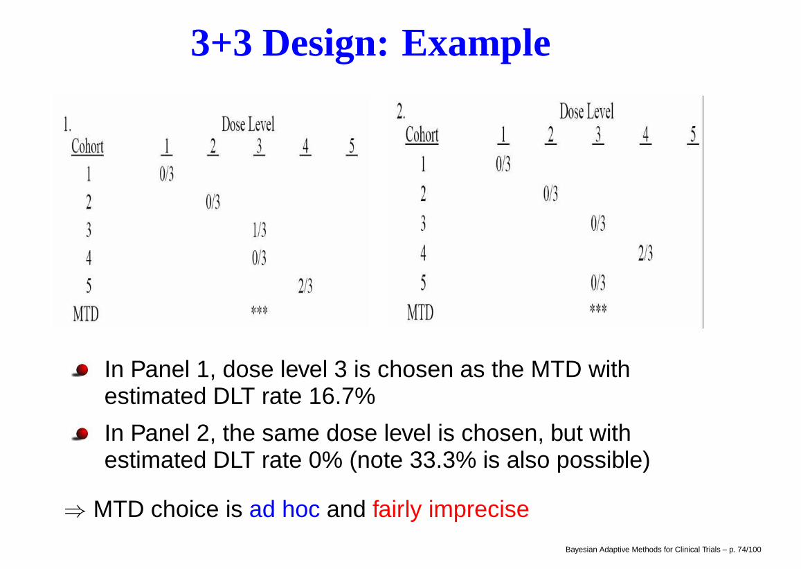
3+3 Design: Example
In Panel 1, dose level 3 is chosen as the MTD withestimated DLT rate 16.7%
In Panel 2, the same dose level is chosen, but withestimated DLT rate 0% (note 33.3% is also possible)
⇒ MTD choice is ad hoc and fairly imprecise
Bayesian Adaptive Methods for Clinical Trials – p. 74/100
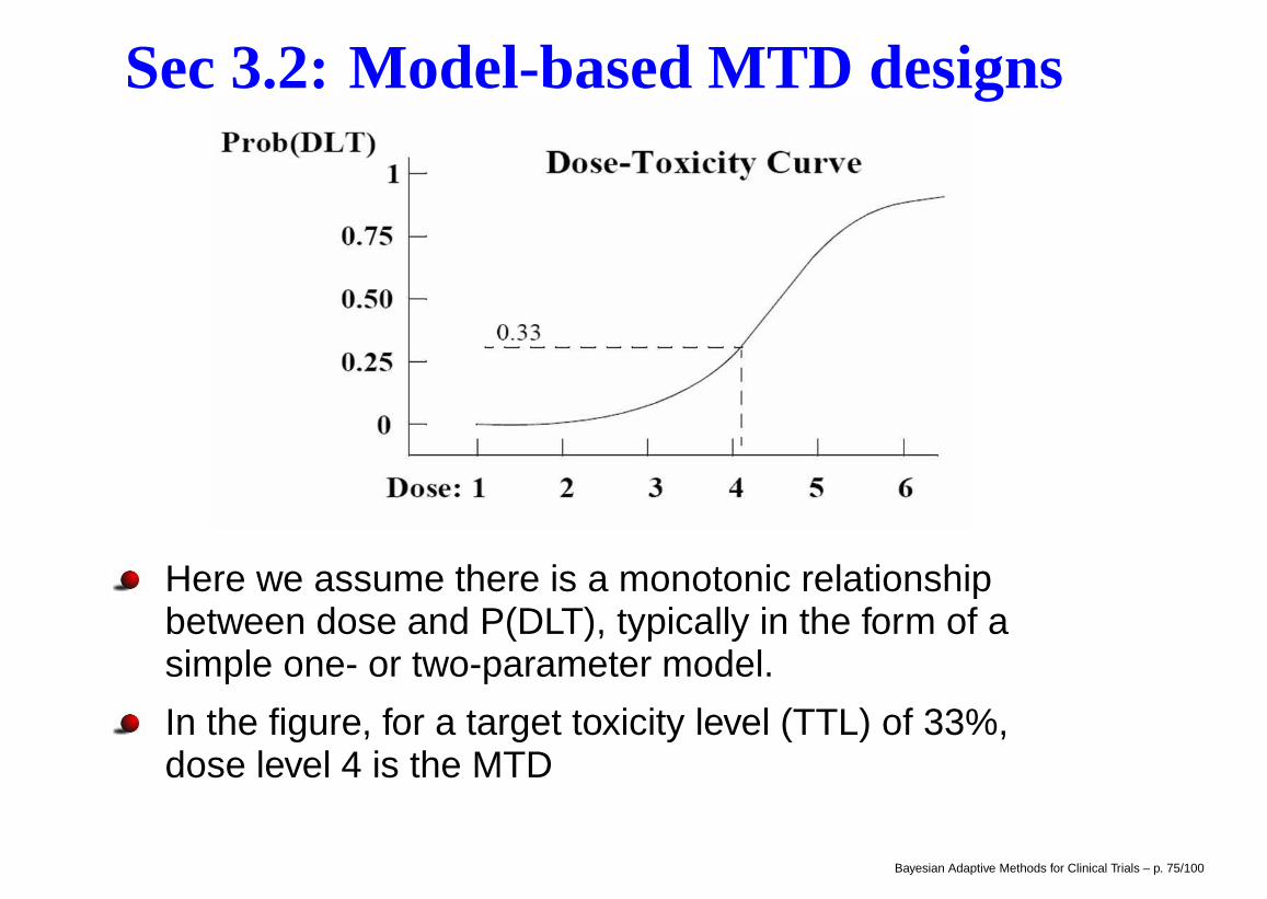
Sec 3.2: Model-based MTD designs
Here we assume there is a monotonic relationshipbetween dose and P(DLT), typically in the form of asimple one- or two-parameter model.
In the figure, for a target toxicity level (TTL) of 33%,dose level 4 is the MTD
Bayesian Adaptive Methods for Clinical Trials – p. 75/100
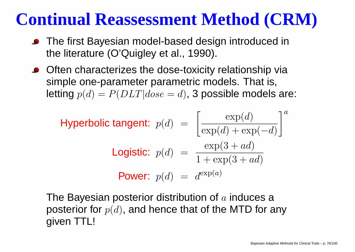
Continual Reassessment Method (CRM)The first Bayesian model-based design introduced inthe literature (O’Quigley et al., 1990).
Often characterizes the dose-toxicity relationship viasimple one-parameter parametric models. That is,letting p(d) = P (DLT |dose = d), 3 possible models are:
Hyperbolic tangent: p(d) =
[exp(d)
exp(d) + exp(−d)
]a
Logistic: p(d) =exp(3 + ad)
1 + exp(3 + ad)
Power: p(d) = dexp(a)
The Bayesian posterior distribution of a induces aposterior for p(d), and hence that of the MTD for anygiven TTL!
Bayesian Adaptive Methods for Clinical Trials – p. 76/100
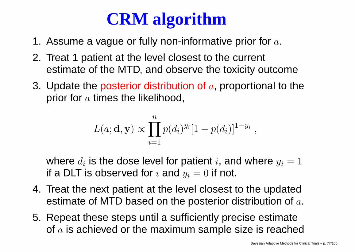
CRM algorithm1. Assume a vague or fully non-informative prior for a.
2. Treat 1 patient at the level closest to the currentestimate of the MTD, and observe the toxicity outcome
3. Update the posterior distribution of a, proportional to theprior for a times the likelihood,
L(a;d,y) ∝n∏
i=1
p(di)yi [1− p(di)]
1−yi ,
where di is the dose level for patient i, and where yi = 1if a DLT is observed for i and yi = 0 if not.
4. Treat the next patient at the level closest to the updatedestimate of MTD based on the posterior distribution of a.
5. Repeat these steps until a sufficiently precise estimateof a is achieved or the maximum sample size is reached
Bayesian Adaptive Methods for Clinical Trials – p. 77/100
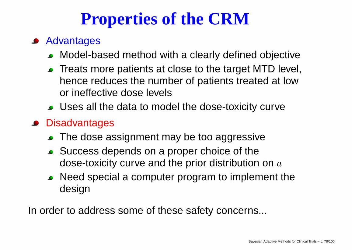
Properties of the CRMAdvantages
Model-based method with a clearly defined objectiveTreats more patients at close to the target MTD level,hence reduces the number of patients treated at lowor ineffective dose levelsUses all the data to model the dose-toxicity curve
DisadvantagesThe dose assignment may be too aggressiveSuccess depends on a proper choice of thedose-toxicity curve and the prior distribution on a
Need special a computer program to implement thedesign
In order to address some of these safety concerns...
Bayesian Adaptive Methods for Clinical Trials – p. 78/100
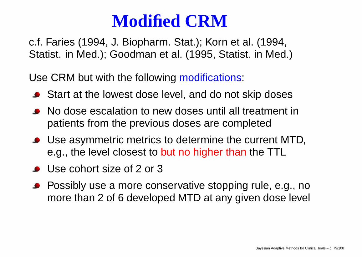
Modified CRMc.f. Faries (1994, J. Biopharm. Stat.); Korn et al. (1994,Statist. in Med.); Goodman et al. (1995, Statist. in Med.)
Use CRM but with the following modifications:
Start at the lowest dose level, and do not skip doses
No dose escalation to new doses until all treatment inpatients from the previous doses are completed
Use asymmetric metrics to determine the current MTD,e.g., the level closest to but no higher than the TTL
Use cohort size of 2 or 3
Possibly use a more conservative stopping rule, e.g., nomore than 2 of 6 developed MTD at any given dose level
Bayesian Adaptive Methods for Clinical Trials – p. 79/100
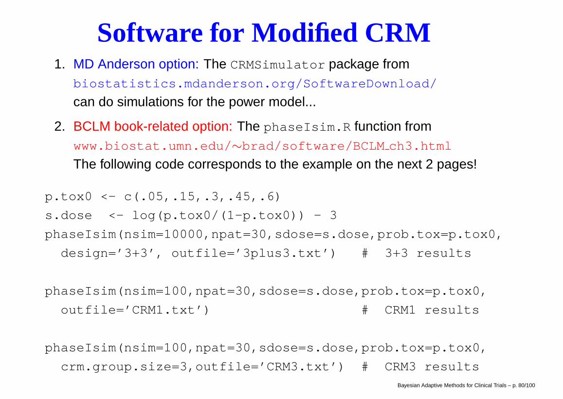
Software for Modified CRM1. MD Anderson option: The CRMSimulator package from
biostatistics.mdanderson.org/SoftwareDownload/
can do simulations for the power model...
2. BCLM book-related option: The phaseIsim.R function fromwww.biostat.umn.edu/∼brad/software/BCLM ch3.html
The following code corresponds to the example on the next 2 pages!
p.tox0 <- c(.05,.15,.3,.45,.6)
s.dose <- log(p.tox0/(1-p.tox0)) - 3
phaseIsim(nsim=10000,npat=30,sdose=s.dose,prob.tox=p.tox0,
design=’3+3’, outfile=’3plus3.txt’) # 3+3 results
phaseIsim(nsim=100,npat=30,sdose=s.dose,prob.tox=p.tox0,
outfile=’CRM1.txt’) # CRM1 results
phaseIsim(nsim=100,npat=30,sdose=s.dose,prob.tox=p.tox0,
crm.group.size=3,outfile=’CRM3.txt’) # CRM3 resultsBayesian Adaptive Methods for Clinical Trials – p. 80/100
Modified CRM outperforms 3+3Suppose that in developing a new agent, we have fivepotential dose levels, and our target toxicity level is30%. We wish to simulate and compare the operatingcharacteristics of the 3+3 and two CRM designs using10,000 simulated trials.
Suppose the true probabilities of DLT at dose levels 1 to5 are 0.05, 0.15, 0.30, 0.45, and 0.60, respectively, sothat dose level 3 is the true MTD.
The table on the next page shows that the CRM designwith a cohort size of 1 (CRM 1) treats more patients atthe true MTD level, but also more patients at dose levelsabove the MTD. The overall percent of DLT for the 3+3and CRM 1 designs are 21.1 and 27.0, respectively.
By increasing the CRM cohort size from 1 to 3 (CRM 3),we treat fewer patients at levels above the MTD.
Bayesian Adaptive Methods for Clinical Trials – p. 81/100
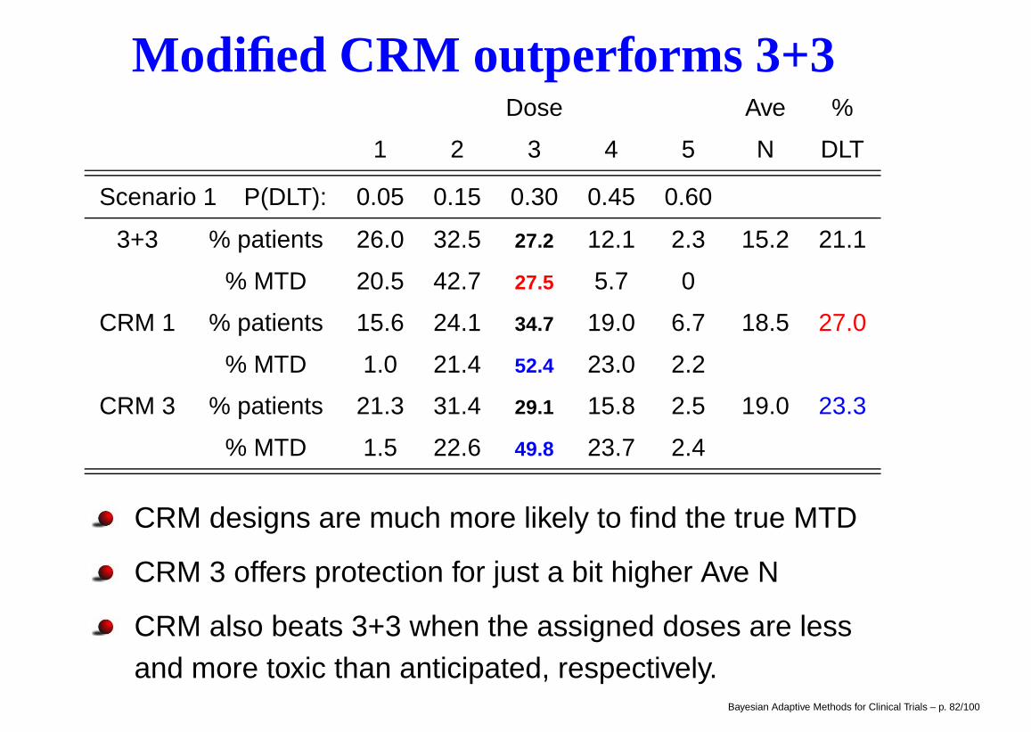
Modified CRM outperforms 3+3Dose Ave %
1 2 3 4 5 N DLT
Scenario 1 P(DLT): 0.05 0.15 0.30 0.45 0.60
3+3 % patients 26.0 32.5 27.2 12.1 2.3 15.2 21.1
% MTD 20.5 42.7 27.5 5.7 0
CRM 1 % patients 15.6 24.1 34.7 19.0 6.7 18.5 27.0
% MTD 1.0 21.4 52.4 23.0 2.2
CRM 3 % patients 21.3 31.4 29.1 15.8 2.5 19.0 23.3
% MTD 1.5 22.6 49.8 23.7 2.4
CRM designs are much more likely to find the true MTD
CRM 3 offers protection for just a bit higher Ave N
CRM also beats 3+3 when the assigned doses are lessand more toxic than anticipated, respectively.
Bayesian Adaptive Methods for Clinical Trials – p. 82/100
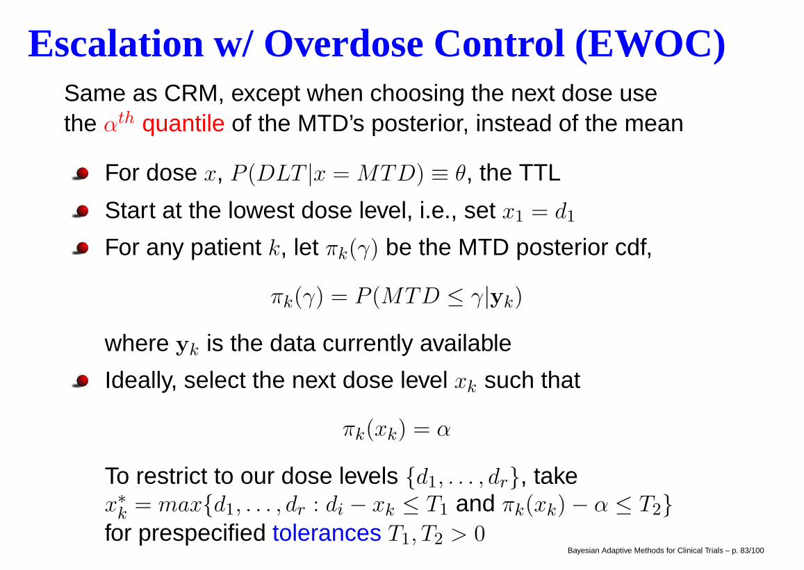
Escalation w/ Overdose Control (EWOC)Same as CRM, except when choosing the next dose usethe αth quantile of the MTD’s posterior, instead of the mean
For dose x, P (DLT |x = MTD) ≡ θ, the TTL
Start at the lowest dose level, i.e., set x1 = d1
For any patient k, let πk(γ) be the MTD posterior cdf,
πk(γ) = P (MTD ≤ γ|yk)
where yk is the data currently available
Ideally, select the next dose level xk such that
πk(xk) = α
To restrict to our dose levels {d1, . . . , dr}, takex∗k = max{d1, . . . , dr : di − xk ≤ T1 and πk(xk)− α ≤ T2}for prespecified tolerances T1, T2 > 0
Bayesian Adaptive Methods for Clinical Trials – p. 83/100
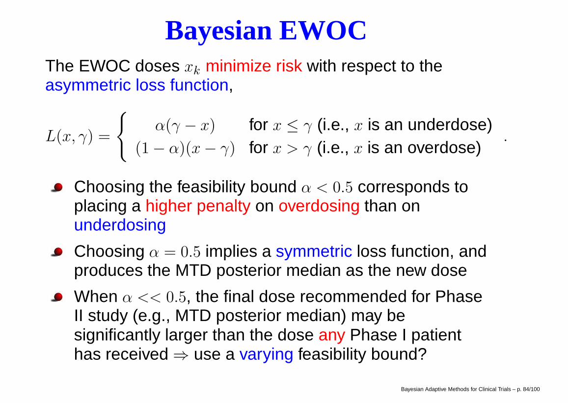
Bayesian EWOCThe EWOC doses xk minimize risk with respect to theasymmetric loss function,
L(x, γ) =
{α(γ − x) for x ≤ γ (i.e., x is an underdose)
(1− α)(x− γ) for x > γ (i.e., x is an overdose).
Choosing the feasibility bound α < 0.5 corresponds toplacing a higher penalty on overdosing than onunderdosing
Choosing α = 0.5 implies a symmetric loss function, andproduces the MTD posterior median as the new dose
When α << 0.5, the final dose recommended for PhaseII study (e.g., MTD posterior median) may besignificantly larger than the dose any Phase I patienthas received ⇒ use a varying feasibility bound?
Bayesian Adaptive Methods for Clinical Trials – p. 84/100
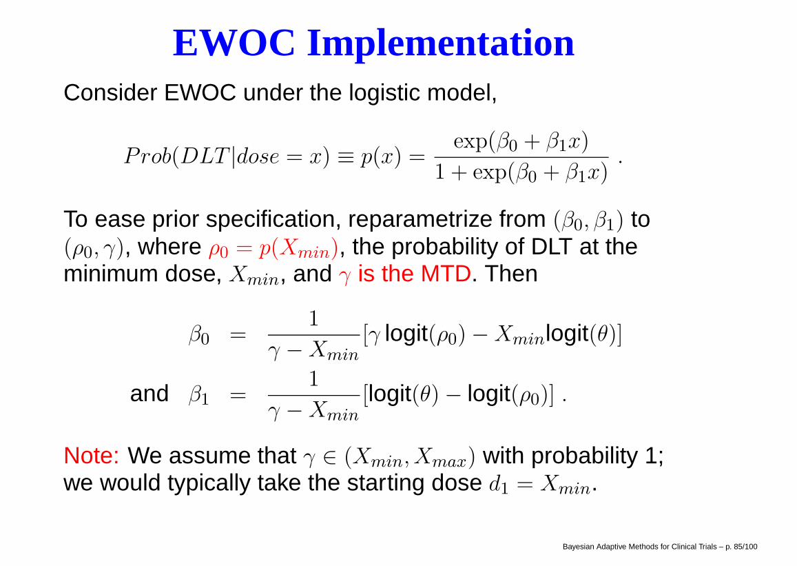
EWOC ImplementationConsider EWOC under the logistic model,
Prob(DLT |dose = x) ≡ p(x) =exp(β0 + β1x)
1 + exp(β0 + β1x).
To ease prior specification, reparametrize from (β0, β1) to(ρ0, γ), where ρ0 = p(Xmin), the probability of DLT at theminimum dose, Xmin, and γ is the MTD. Then
β0 =1
γ −Xmin[γ logit(ρ0)−Xminlogit(θ)]
and β1 =1
γ −Xmin[logit(θ)− logit(ρ0)] .
Note: We assume that γ ∈ (Xmin, Xmax) with probability 1;we would typically take the starting dose d1 = Xmin.
Bayesian Adaptive Methods for Clinical Trials – p. 85/100
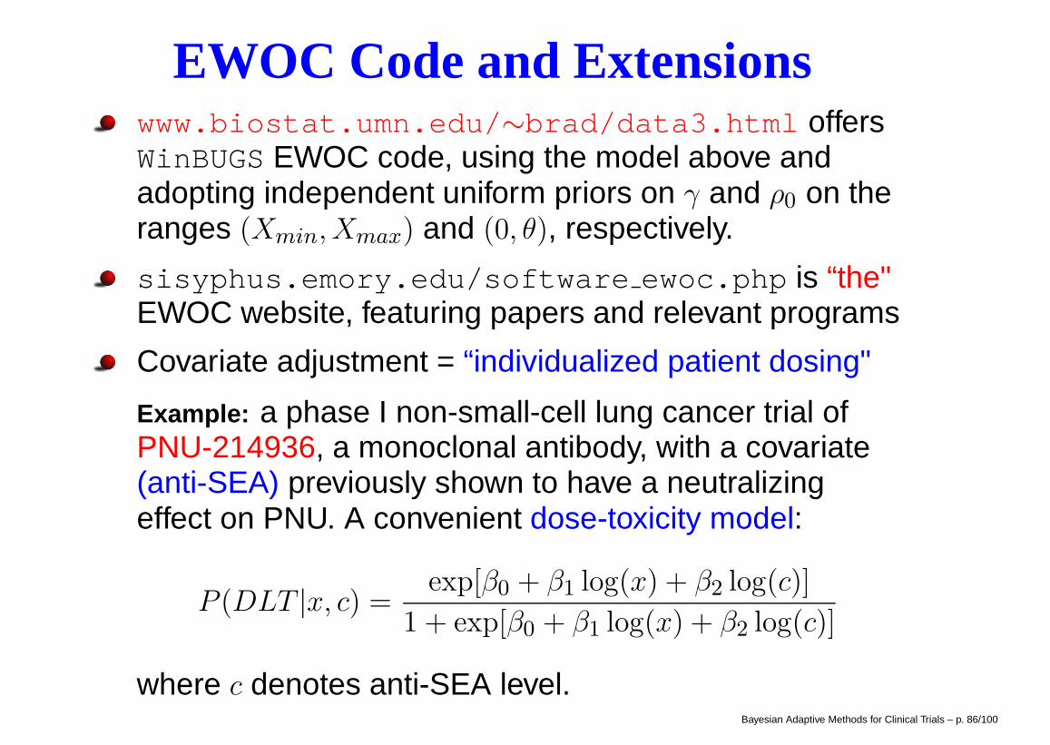
EWOC Code and Extensionswww.biostat.umn.edu/∼brad/data3.html offersWinBUGS EWOC code, using the model above andadopting independent uniform priors on γ and ρ0 on theranges (Xmin, Xmax) and (0, θ), respectively.
sisyphus.emory.edu/software ewoc.php is “the"EWOC website, featuring papers and relevant programs
Covariate adjustment = “individualized patient dosing"
Example: a phase I non-small-cell lung cancer trial ofPNU-214936, a monoclonal antibody, with a covariate(anti-SEA) previously shown to have a neutralizingeffect on PNU. A convenient dose-toxicity model:
P (DLT |x, c) = exp[β0 + β1 log(x) + β2 log(c)]
1 + exp[β0 + β1 log(x) + β2 log(c)]
where c denotes anti-SEA level.Bayesian Adaptive Methods for Clinical Trials – p. 86/100

EWOC ExtensionsRecent work by Zabor (2010) considers the case of twocovariates, one categorical and one continuous
Example: Trial of 852A, an “agonist" that can enhancethe tumor-inhibiting and immune response-boostingproperties of other oncologic agents. Let z be 0 formale, 1 for female, and let c ∈ [39, 80] be the patient’sage in years. Then our model for P (DLT ) is
P (DLT |x, c, z) = exp[β0 + β1x+ β2c+ β3z]
1 + exp[β0 + β1x+ β2c+ β3z].
Reparametrize to γmax = γ(c = 80, z = 0) and
ρ1 = P (DLT |X = Xmin, C = 39, Z = 0)
ρ2 = P (DLT |X = Xmin, C = 80, Z = 0)
ρ3 = P (DLT |X = Xmin, C = 39, Z = 1)
Bayesian Adaptive Methods for Clinical Trials – p. 87/100
EWOC Results
0.0
0.2
0.4
0.6
0.8
1.0
Dose
P(D
LT)
0.15
0.30
0.60
1.20
1.55
2.00
θ
Males
39−6465−7475−80
0.0
0.2
0.4
0.6
0.8
1.0
Dose
P(D
LT)
0.15
0.30
0.60
1.20
1.55
2.00
θ
Females
39−6465−7475−80
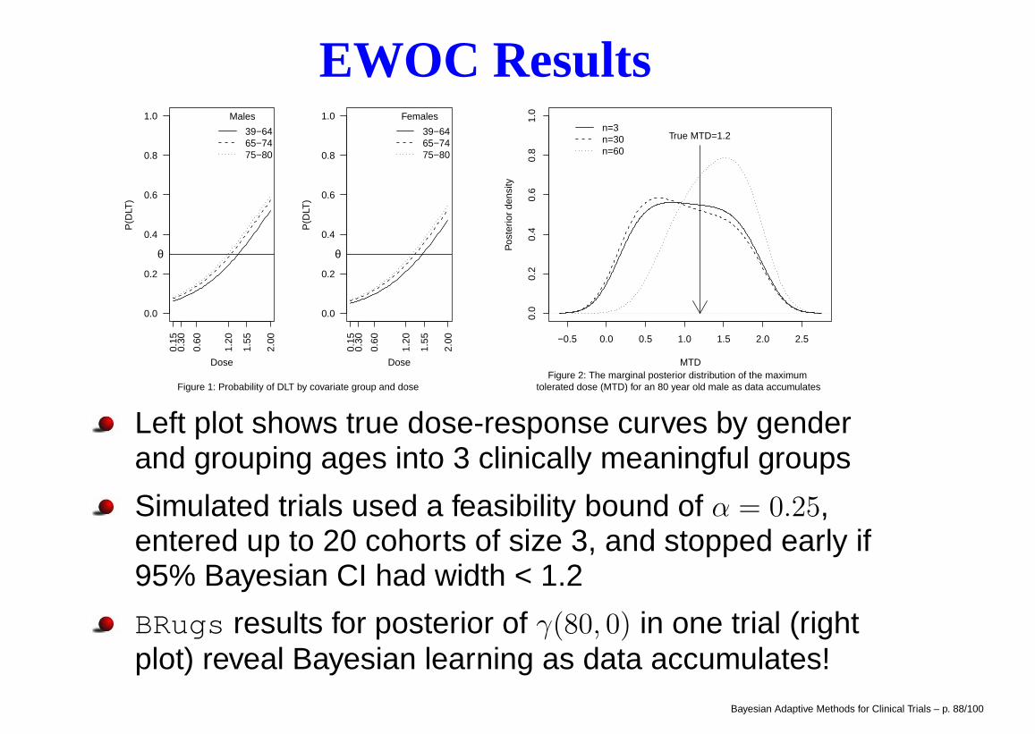
Figure 1: Probability of DLT by covariate group and dose
−0.5 0.0 0.5 1.0 1.5 2.0 2.5
0.0
0.2
0.4
0.6
0.8
1.0
MTD
Pos
terio
r de
nsity
True MTD=1.2n=3n=30n=60
Figure 2: The marginal posterior distribution of the maximum tolerated dose (MTD) for an 80 year old male as data accumulates
Left plot shows true dose-response curves by genderand grouping ages into 3 clinically meaningful groups
Simulated trials used a feasibility bound of α = 0.25,entered up to 20 cohorts of size 3, and stopped early if95% Bayesian CI had width < 1.2
BRugs results for posterior of γ(80, 0) in one trial (rightplot) reveal Bayesian learning as data accumulates!
Bayesian Adaptive Methods for Clinical Trials – p. 88/100
Outline
Session II (cont.)– TITE-CRM– Efficacy - Toxicity Trade-off (EffTox)– Combination Therapy
Session III (Phase II Studies)– Standard phase IIA Designs– Predictive Probability-Based Methods– Posterior Probability-Based Methods
Stopping for futility and efficacyStopping for futility, efficacy, and toxicity
– Adaptive Randomization (AR)Baseline ARResponse (Outcome-based) AR
– Biomarker-based Adaptive Design (BATTLE)1
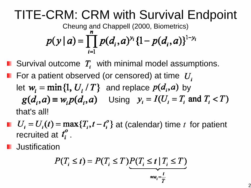
TITE-CRM: CRM with Survival EndpointCheung and Chappell (2000, Biometrics)
Survival outcome with minimal model assumptions.For a patient observed (or censored) at time let and replace by
Using that's all!
at (calendar) time t for patient recruited at .Justification
2
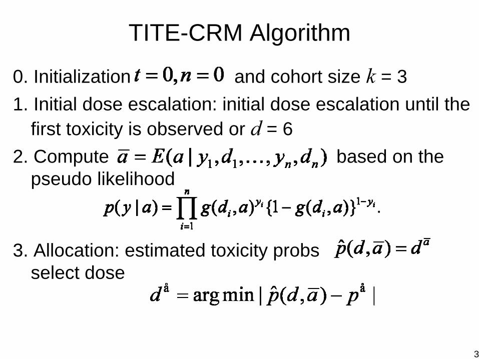
TITE-CRM Algorithm
0. Initialization and cohort size k = 31. Initial dose escalation: initial dose escalation until the
first toxicity is observed or d = 62. Compute based on the
pseudo likelihood
3. Allocation: estimated toxicity probsselect dose
3
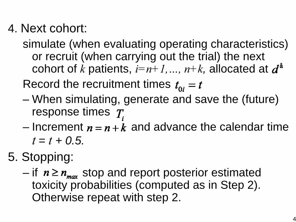
4. Next cohort:simulate (when evaluating operating characteristics)
or recruit (when carrying out the trial) the next cohort of k patients, i=n+1,…, n+k, allocated at
Record the recruitment times– When simulating, generate and save the (future)
response times – Increment and advance the calendar time
t = t + 0.5.5. Stopping:
– if stop and report posterior estimated toxicity probabilities (computed as in Step 2). Otherwise repeat with step 2.
4

Compute the Posterior of aEvaluating evaluate the posterior expectation as average over a grid:Posterior expectation:
sum over a grid.Grid:Evaluate the pointwise posterior
and compute
5
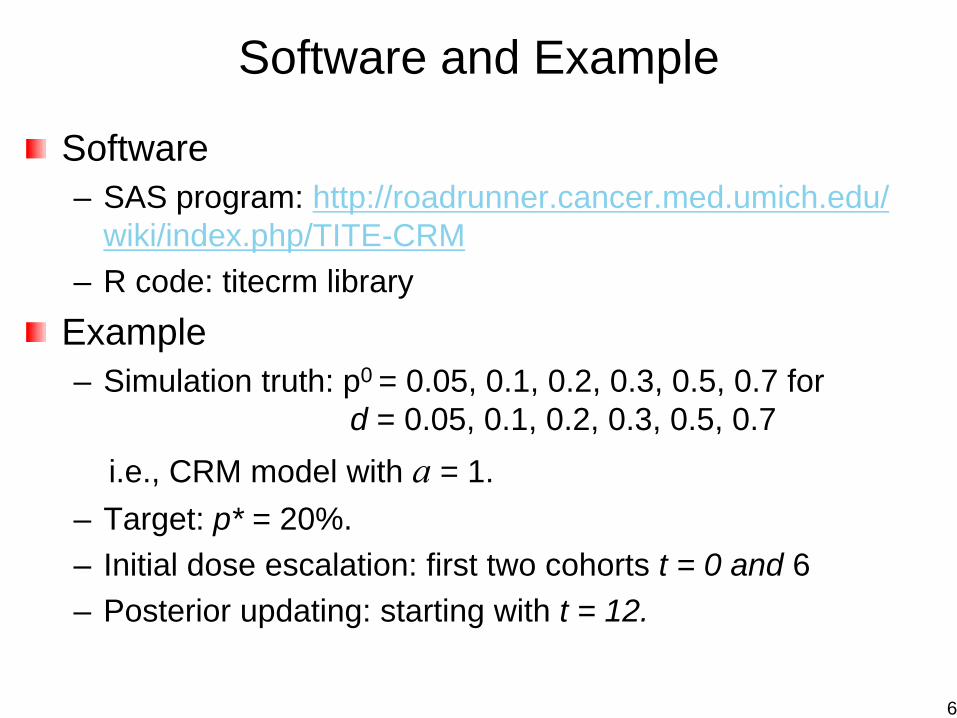
Software and Example
Software– SAS program: http://roadrunner.cancer.med.umich.edu/
wiki/index.php/TITE-CRM– R code: titecrm library
Example– Simulation truth: p0 = 0.05, 0.1, 0.2, 0.3, 0.5, 0.7 for
d = 0.05, 0.1, 0.2, 0.3, 0.5, 0.7 i.e., CRM model with a = 1.
– Target: p* = 20%.– Initial dose escalation: first two cohorts t = 0 and 6– Posterior updating: starting with t = 12.
6
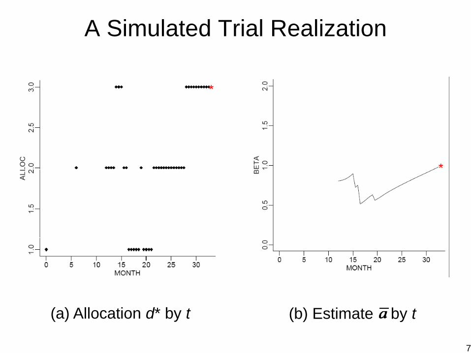
A Simulated Trial Realization
(a) Allocation d* by t (b) Estimate by t
7

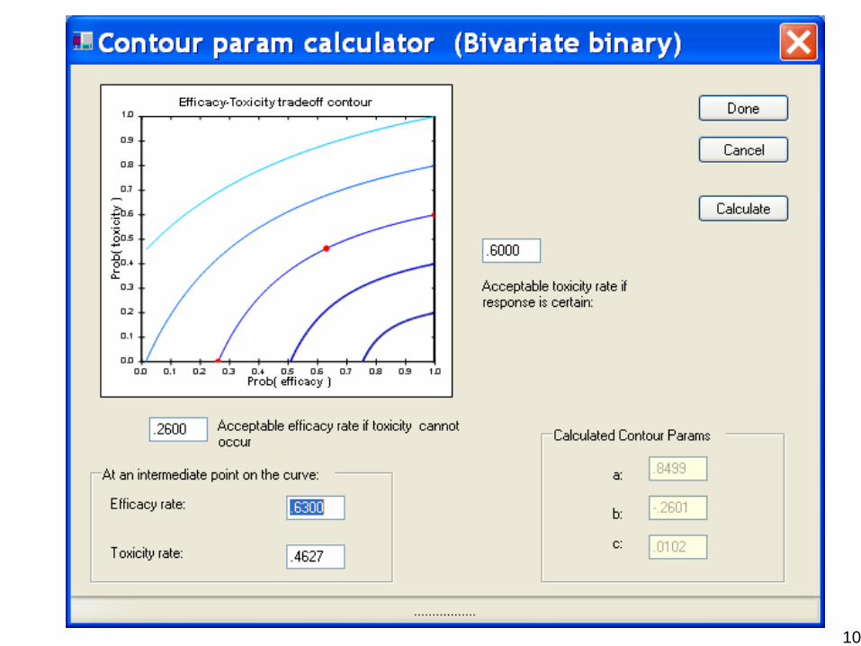
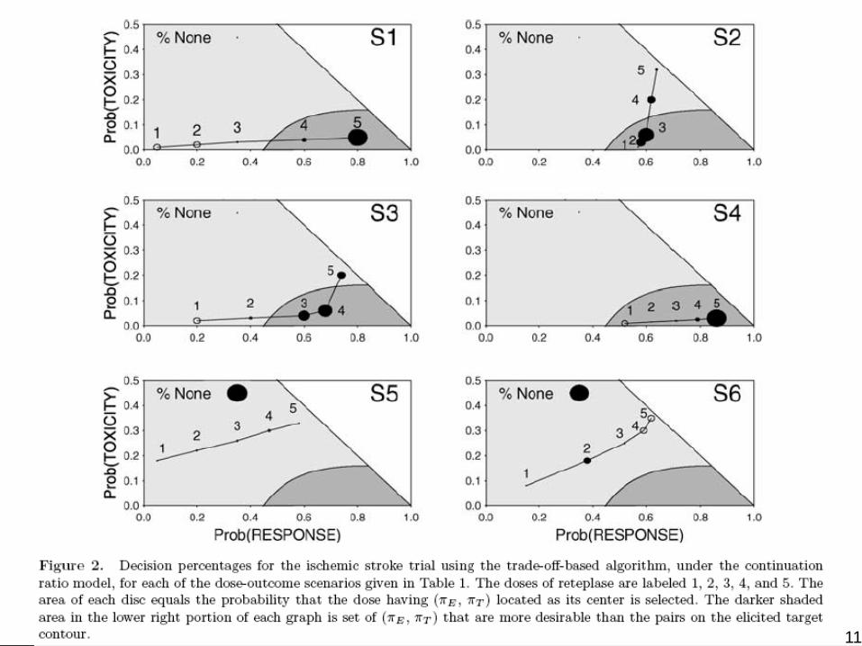
Dose-Finding Based On Efficacy-Toxicity Trade-OffsThall and Cook, Biometrics 60:684-693, 2004
Patient Outcome = {Efficacy, Toxicity}
The physician must specify – A Lower Limit pE* on πE = Pr(Efficacy)– An Upper Limit pT* on πT = Pr(Tox)– Three equally desirable(πE, πT) targets to construct an
Efficacy -Toxicity Trade-off ContourA dose x is acceptable if e.g.,
Pr{ πE(x,θ) > pE* | data } > .90
Pr{ πT(x,θ) < pT* | data } > .90
Given the current data, compute the posterior prob of πE and πT to determine the dose level of the next patient
8
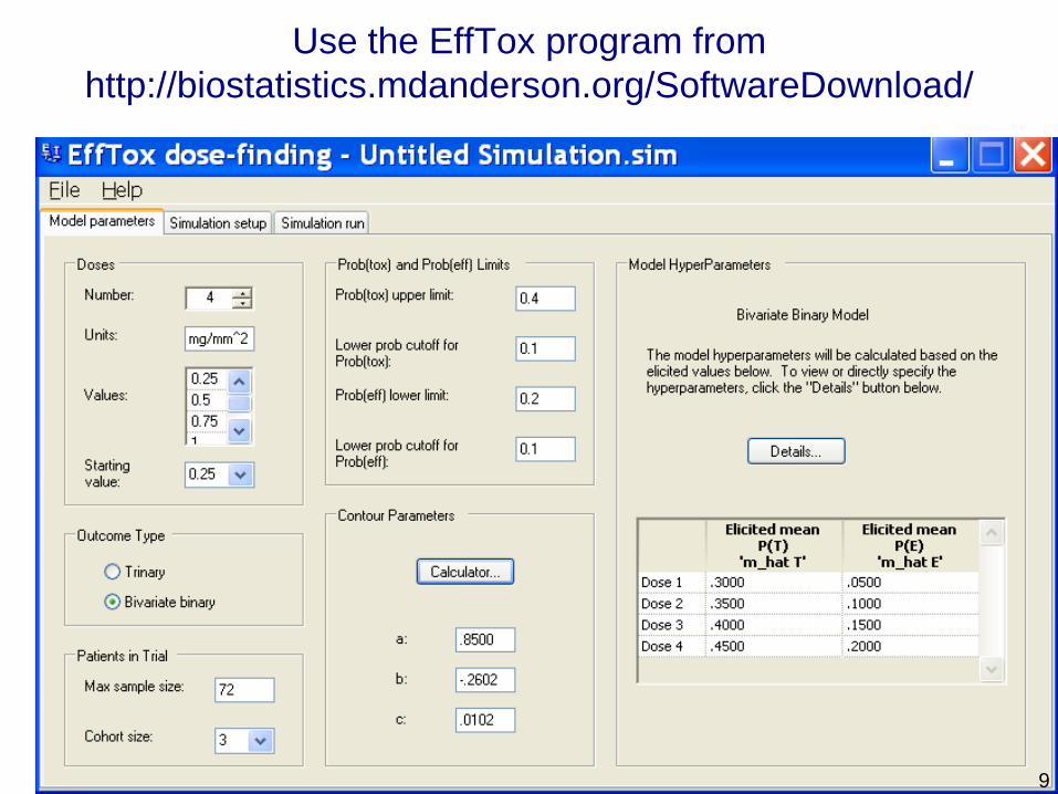
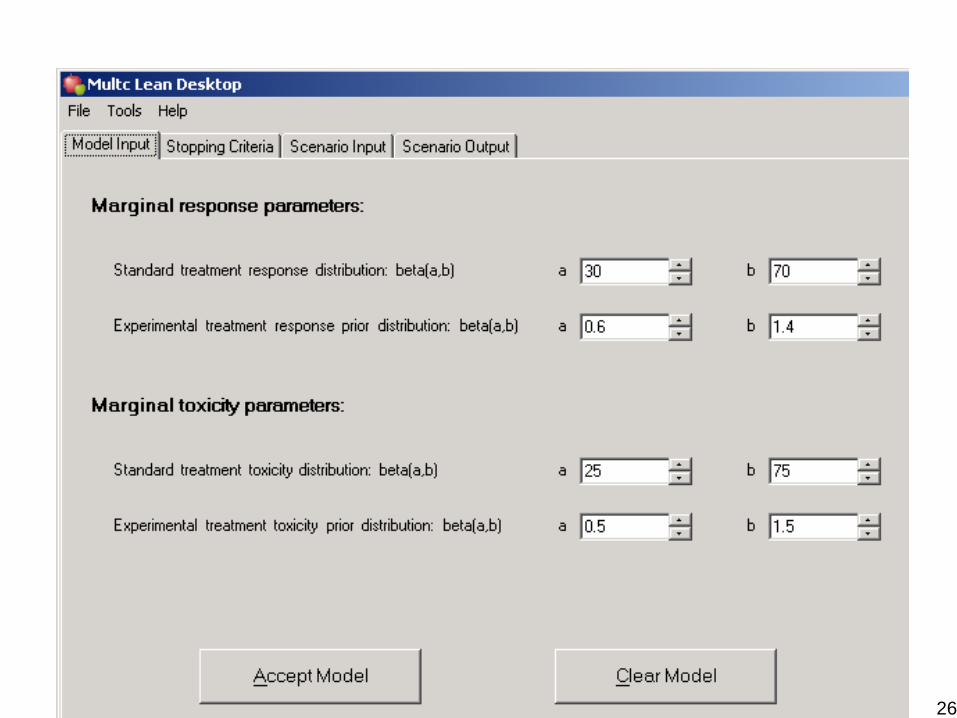
Use the EffTox program from http://biostatistics.mdanderson.org/SoftwareDownload/
9
10
11
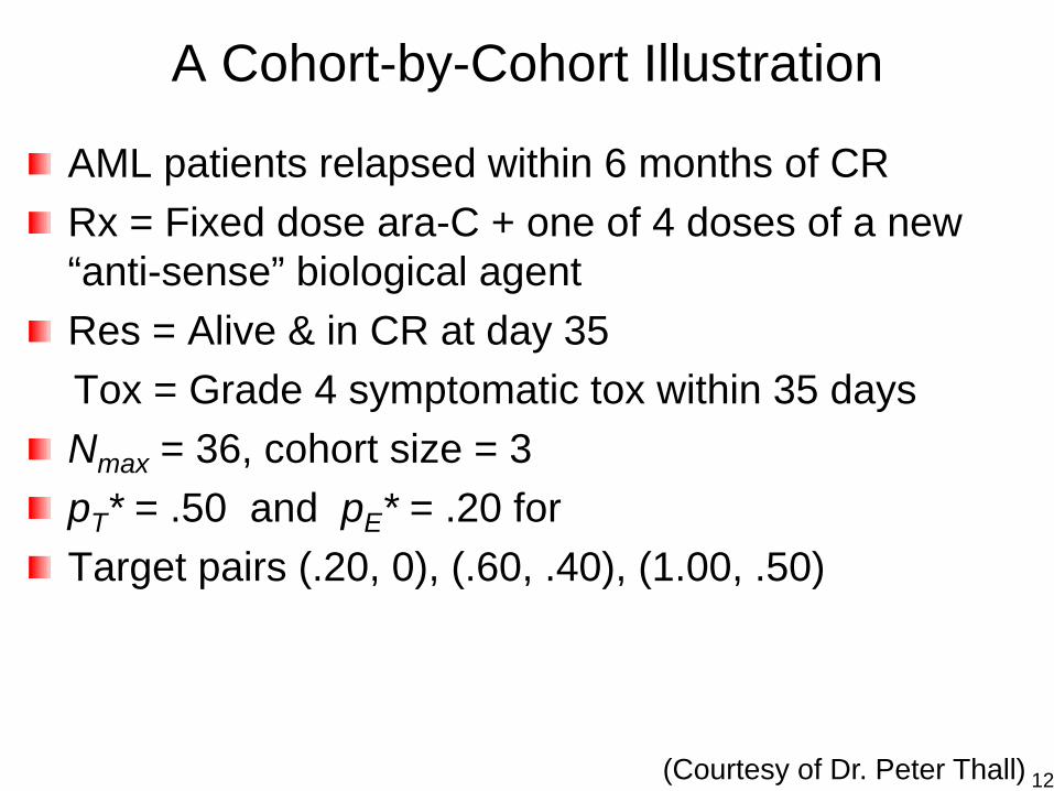
A Cohort-by-Cohort Illustration
AML patients relapsed within 6 months of CRRx = Fixed dose ara-C + one of 4 doses of a new “anti-sense” biological agent Res = Alive & in CR at day 35Tox = Grade 4 symptomatic tox within 35 daysNmax = 36, cohort size = 3pT* = .50 and pE* = .20 for Target pairs (.20, 0), (.60, .40), (1.00, .50)
(Courtesy of Dr. Peter Thall) 12
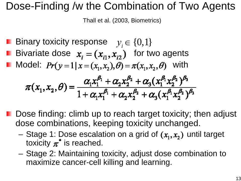
Dose-Finding /w the Combination of Two AgentsThall et al. (2003, Biometrics)
Binary toxicity responseBivariate dose for two agentsModel: with
Dose finding: climb up to reach target toxicity; then adjust dose combinations, keeping toxicity unchanged.– Stage 1: Dose escalation on a grid of until target
toxicity is reached.– Stage 2: Maintaining toxicity, adjust dose combination to
maximize cancer-cell killing and learning.
{0,1}iy ∈
13
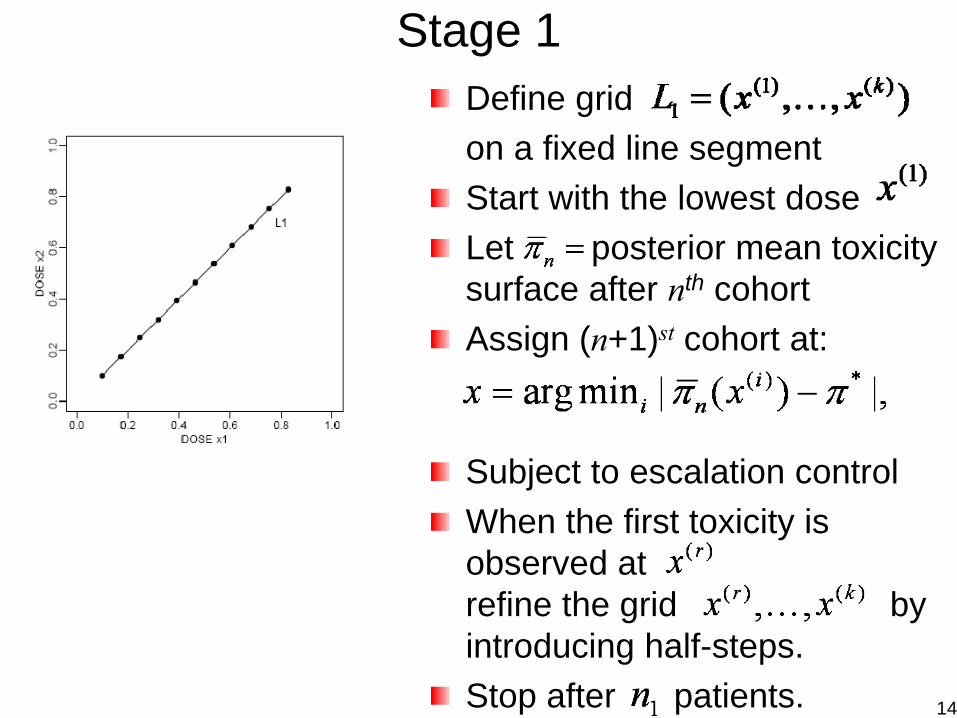
Stage 1Define grid on a fixed line segmentStart with the lowest doseLet posterior mean toxicity surface after nth cohortAssign (n+1)st cohort at:
Subject to escalation controlWhen the first toxicity is observed atrefine the grid by introducing half-steps.Stop after patients. 14
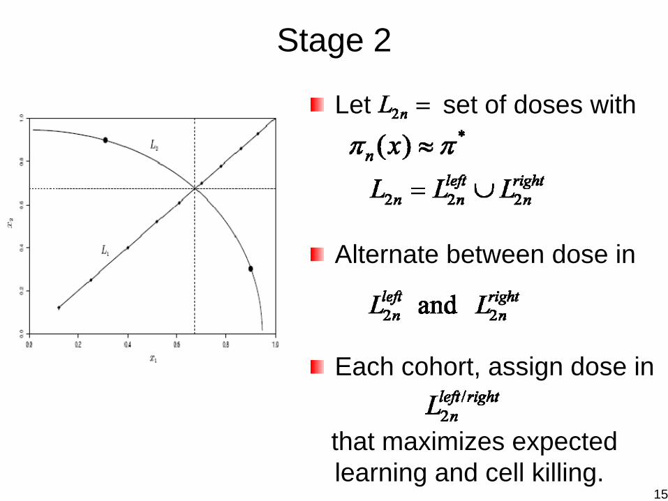
Stage 2
Let set of doses with
Alternate between dose in
Each cohort, assign dose in
that maximizes expected learning and cell killing.
15
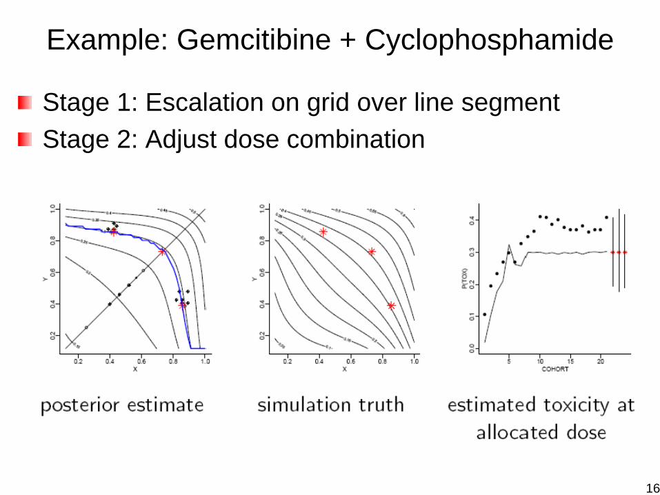
Example: Gemcitibine + Cyclophosphamide
Stage 1: Escalation on grid over line segmentStage 2: Adjust dose combination
16
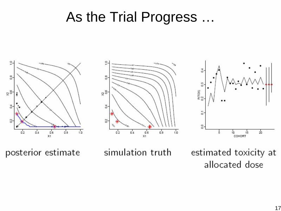
As the Trial Progress …
17
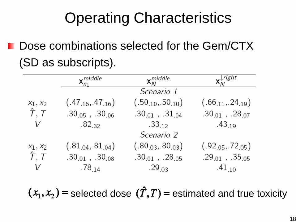
Operating Characteristics
Dose combinations selected for the Gem/CTX (SD as subscripts).
selected dose; estimated and true toxicity,V = posterior uncertainty
18
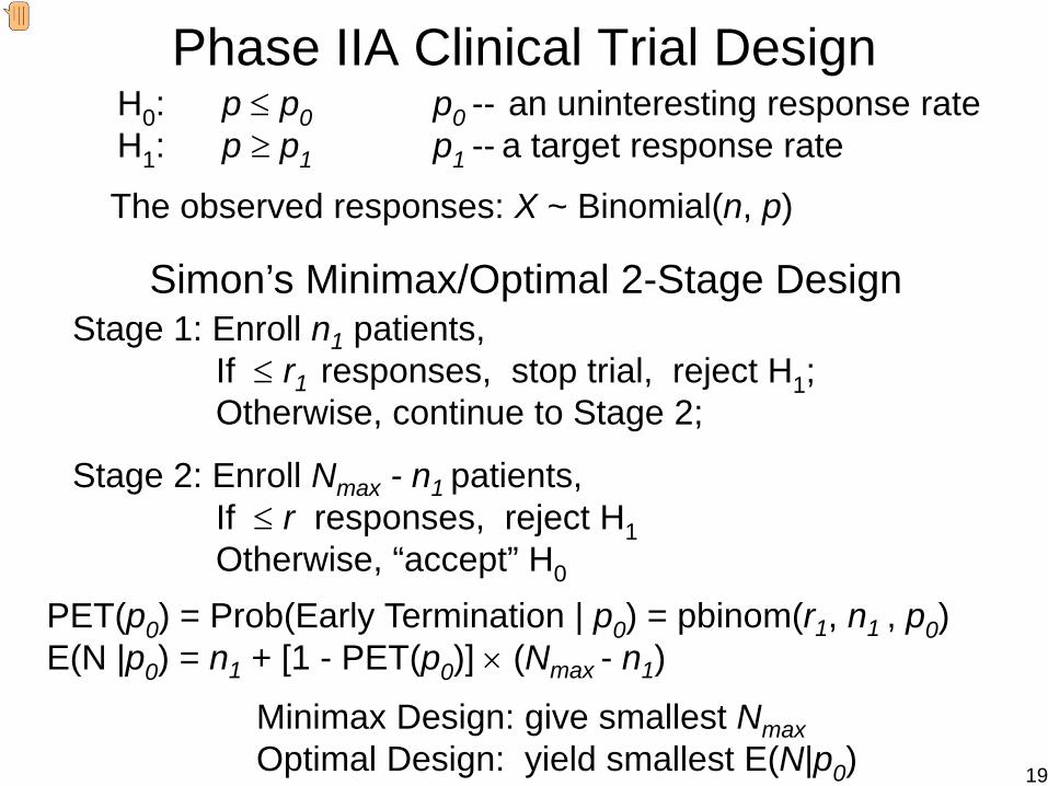
Phase IIA Clinical Trial DesignH0: p ≤ p0 p0 -- an uninteresting response rateH1: p ≥ p1 p1 -- a target response rate
The observed responses: X ~ Binomial(n, p)
Simon’s Minimax/Optimal 2-Stage DesignStage 1: Enroll n1 patients,
If ≤ r1 responses, stop trial, reject H1;Otherwise, continue to Stage 2;
Stage 2: Enroll Nmax - n1 patients, If ≤ r responses, reject H1Otherwise, “accept” H0
PET(p0) = Prob(Early Termination | p0) = pbinom(r1, n1 , p0)E(N |p0) = n1 + [1 - PET(p0)] × (Nmax - n1)
Minimax Design: give smallest NmaxOptimal Design: yield smallest E(N|p0) 19
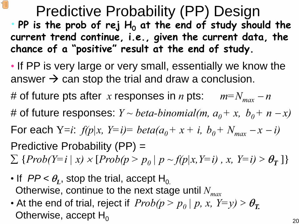
Predictive Probability (PP) Design• PP is the prob of rej H0 at the end of study should the current trend continue, i.e., given the current data, the chance of a “positive” result at the end of study.
• If PP is very large or very small, essentially we know the answer can stop the trial and draw a conclusion.# of future pts after x responses in n pts: m=Nmax − n# of future responses: Y ~ beta-binomial(m, a0 + x, b0 + n − x)For each Y=i: f(p|x, Y=i)= beta(a0 + x + i, b0 + Nmax − x − i)Predictive Probability (PP) =∑ {Prob(Y=i | x) × [Prob(p > p0 | p ~ f(p|x,Y=i) , x, Y=i) > θT ]}
• If PP < θL, stop the trial, accept H0. Otherwise, continue to the next stage until Nmax
• At the end of trial, reject if Prob(p > p0 | p, x, Y=y) > θT. Otherwise, accept H0 20

PP Designs
Goal: Find θL , θT , and Nmax to satisfying the type I and type II error rates constraints.Properties:
1. PP design can control type I and type II error rates while allow interim monitoring.
2. Under H0, PP design can yield a higher PET(p0), and smaller E(N|p0) or Nmax than Simon’s 2-stage design
3. PP design produces a flexible monitoring schedule with robust operating characteristics across a wide range of stages and cohort sizes.
4. Advantages of PP design compared to standard multi-stage design:
More flexible, More efficient, More robust21
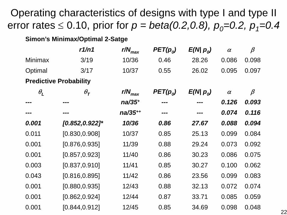
Operating characteristics of designs with type I and type II error rates ≤ 0.10, prior for p = beta(0.2,0.8), p0=0.2, p1=0.4
Simon’s Minimax/Optimal 2-Satger1/n1 r/Nmax PET(p0) E(N| p0) α β
Minimax 3/19 10/36 0.46 28.26 0.086 0.098Optimal 3/17 10/37 0.55 26.02 0.095 0.097Predictive Probability
θL θT r/Nmax PET(p0) E(N| p0) α β
--- --- na/35+ --- --- 0.126 0.093--- --- na/35++ --- --- 0.074 0.1160.001 [0.852,0.922]* 10/36 0.86 27.67 0.088 0.0940.011 [0.830,0.908] 10/37 0.85 25.13 0.099 0.0840.001 [0.876,0.935] 11/39 0.88 29.24 0.073 0.0920.001 [0.857,0.923] 11/40 0.86 30.23 0.086 0.0750.003 [0.837,0.910] 11/41 0.85 30.27 0.100 0.0620.043 [0.816,0.895] 11/42 0.86 23.56 0.099 0.0830.001 [0.880,0.935] 12/43 0.88 32.13 0.072 0.0740.001 [0.862,0.924] 12/44 0.87 33.71 0.085 0.0590.001 [0.844,0.912] 12/45 0.85 34.69 0.098 0.048
22
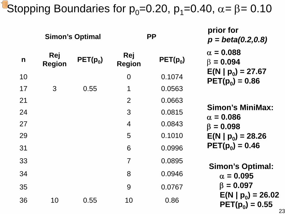
prior for p = beta(0.2,0.8)Simon’s Optimal PP
n Rej Region PET(p0)
Rej Region PET(p0)
10 0 0.107417 3 0.55 1 0.056321 2 0.066324 3 0.081527 4 0.084329 5 0.1010
31 6 0.0996
33 7 0.0895
34 8 0.0946
35 9 0.0767
36 10 0.55 10 0.86
α = 0.088 β = 0.094E(N | p0) = 27.67PET(p0) = 0.86
Simon’s Optimal: α = 0.095 β = 0.097E(N | p0) = 26.02PET(p0) = 0.55
Simon’s MiniMax:α = 0.086β = 0.098E(N | p0) = 28.26PET(p0) = 0.46
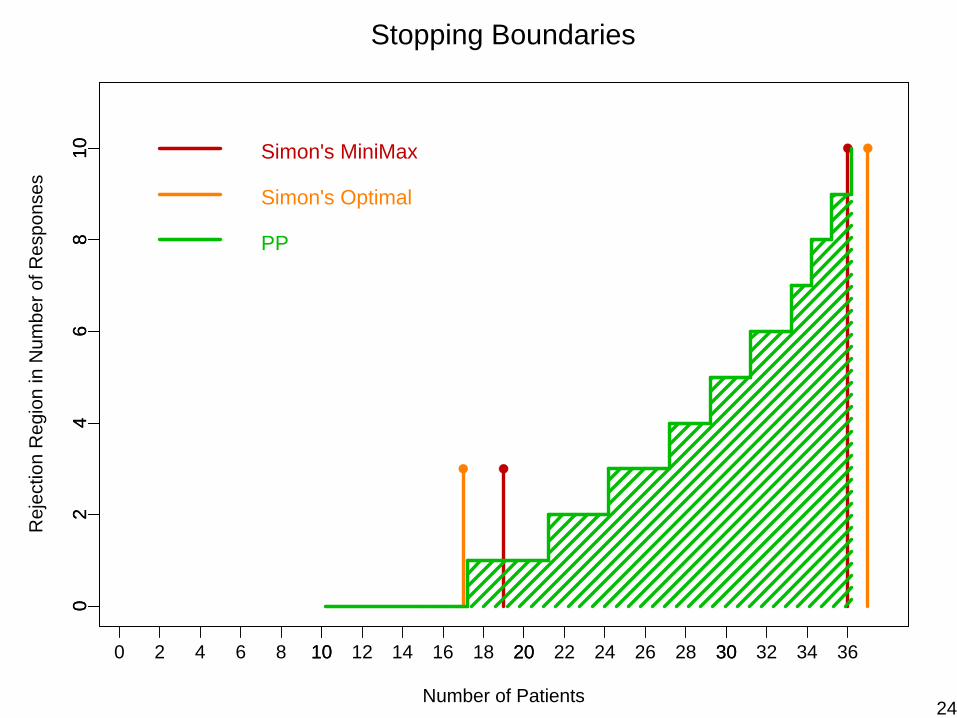
Stopping Boundaries for p0=0.20, p1=0.40, α= β= 0.10
23
Number of Patients
Rej
ectio
n R
egio
n in
Num
ber o
f Res
pons
es
0 10 20 30
02
46
810
2 4 6 8 10 12 14 16 18 20 22 24 26 28 30 32 34 36
02
46
810 Simon's MiniMax
Stopping Boundaries
Simon's Optimal
PP
24
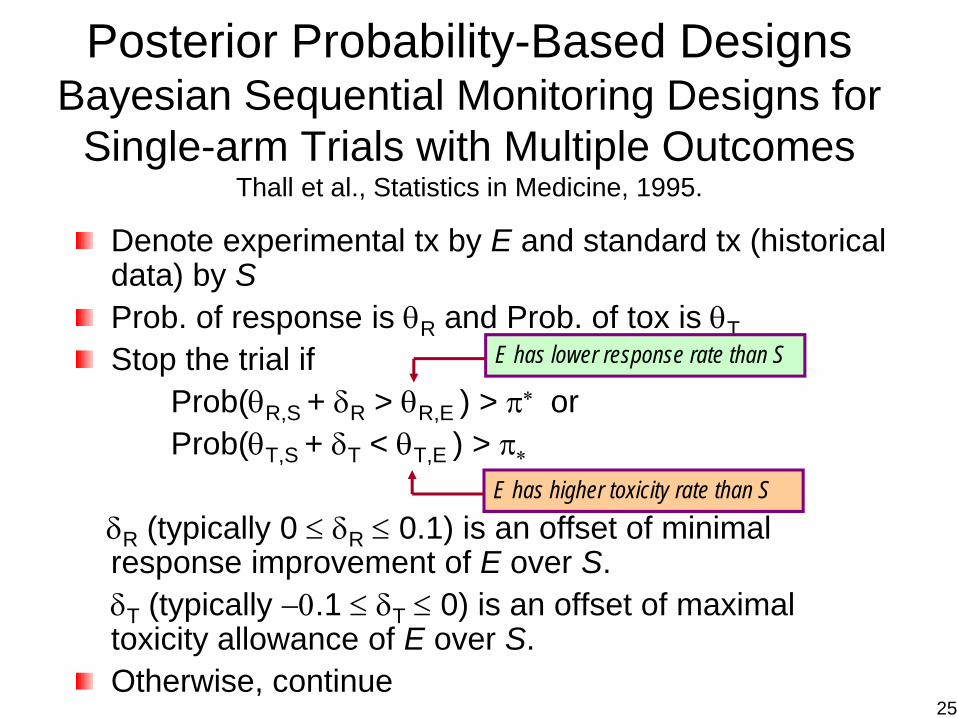
Posterior Probability-Based DesignsBayesian Sequential Monitoring Designs for
Single-arm Trials with Multiple OutcomesThall et al., Statistics in Medicine, 1995.
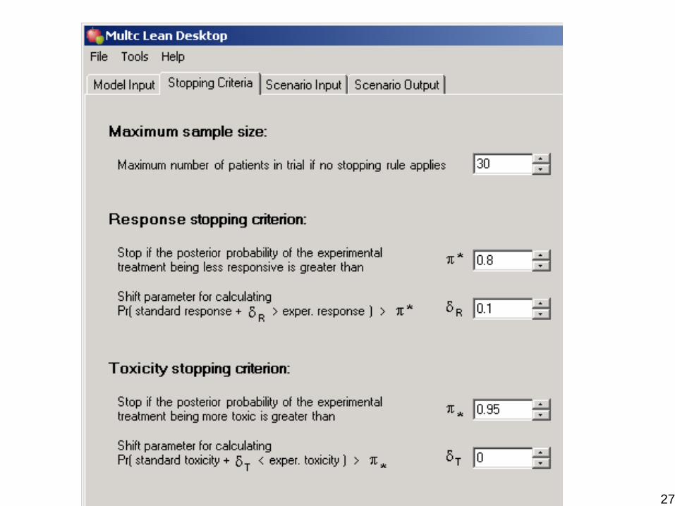
Denote experimental tx by E and standard tx (historical data) by SProb. of response is θR and Prob. of tox is θTStop the trial if
Prob(θR,S + δR > θR,E ) > π∗ orProb(θT,S + δT < θT,E ) > π∗
δR (typically 0 ≤ δR ≤ 0.1) is an offset of minimal response improvement of E over S. δT (typically −0.1 ≤ δT ≤ 0) is an offset of maximal toxicity allowance of E over S. Otherwise, continue
E has lower response rate than S
E has higher toxicity rate than S
25
26
27
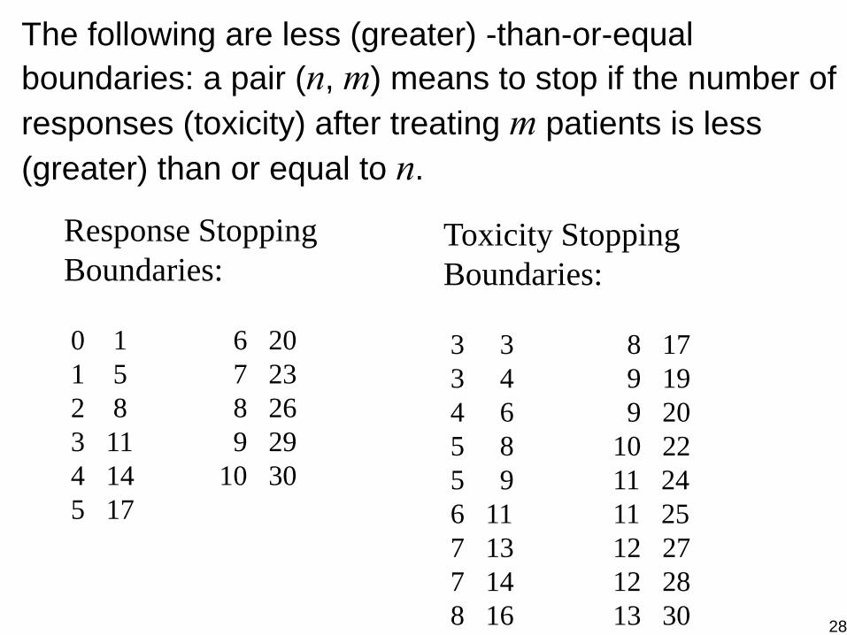
Response Stopping Boundaries:
0 1 6 201 5 7 232 8 8 263 11 9 294 14 10 305 17
Toxicity Stopping Boundaries:
3 3 8 173 4 9 194 6 9 205 8 10 225 9 11 246 11 11 257 13 12 277 14 12 288 16 13 30
The following are less (greater) -than-or-equal boundaries: a pair (n, m) means to stop if the number of responses (toxicity) after treating m patients is less (greater) than or equal to n.
28
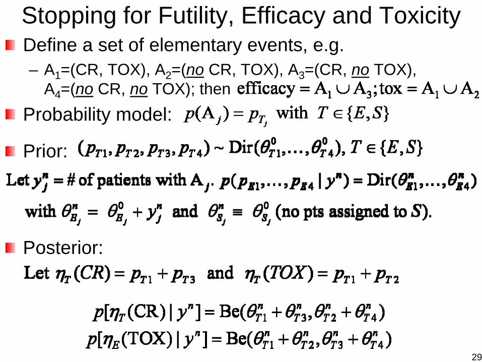
Stopping for Futility, Efficacy and ToxicityDefine a set of elementary events, e.g.– A1=(CR, TOX), A2=(no CR, TOX), A3=(CR, no TOX),
A4=(no CR, no TOX); thenProbability model:
Prior:
Posterior:
29
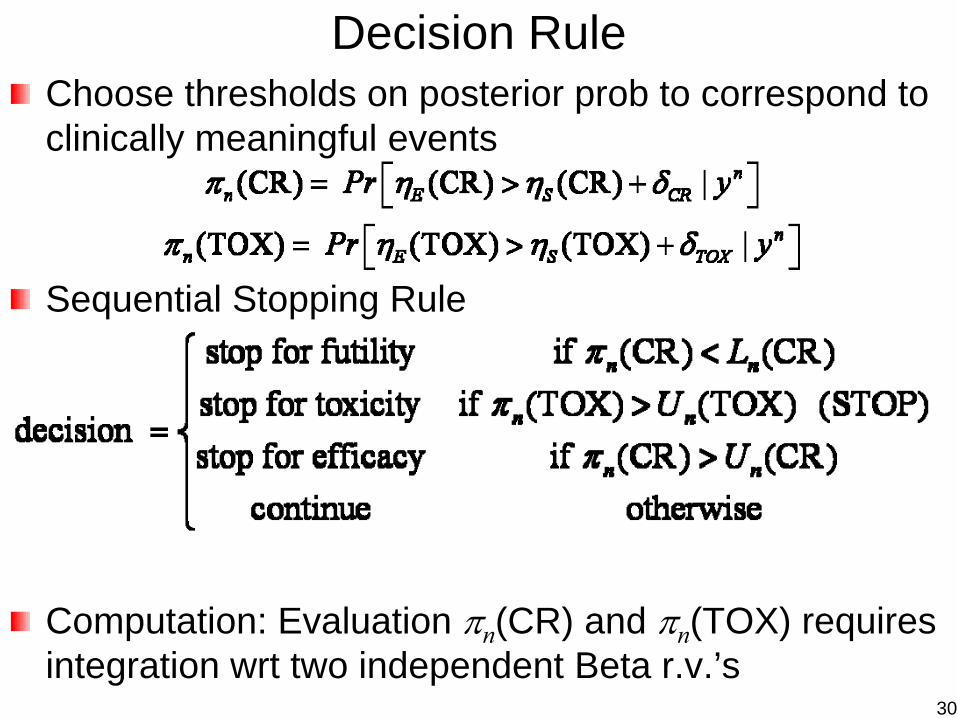
Decision RuleChoose thresholds on posterior prob to correspond to clinically meaningful events
Sequential Stopping Rule
Computation: Evaluation πn(CR) and πn(TOX) requires integration wrt two independent Beta r.v.’s
30
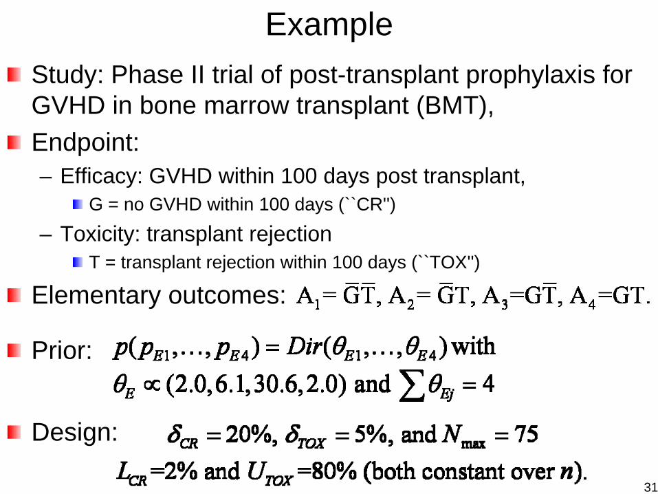
ExampleStudy: Phase II trial of post-transplant prophylaxis for GVHD in bone marrow transplant (BMT), Endpoint: – Efficacy: GVHD within 100 days post transplant,
G = no GVHD within 100 days (``CR'')
– Toxicity: transplant rejectionT = transplant rejection within 100 days (``TOX'')
Elementary outcomes:
Prior:
Design:
31
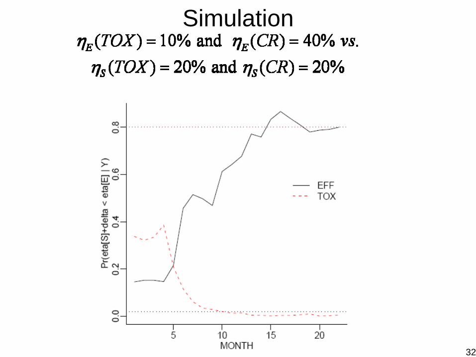
Simulation
32
Adaptive Randomization (AR)(Equal or Adaptive) Randomization Is A Good Thing– Result in comparable study groups wrt known/unknown
prognostic factors– removes investigator bias in the treatment allocation– guarantees the validity of statistical tests
Baseline AR– Ensure balance in prognostic factors among treatment
groups– Based on baseline covariates (static)– Treatment allocation method
Biased coin, urn designPocock-Simon (1975), Minimization
Response (Outcome-based) AR– Allocate more patients in superior treatments and less
patients in inferior treatment based on the observed data – Play the winner - deterministic– Model-based - probabilistic 33
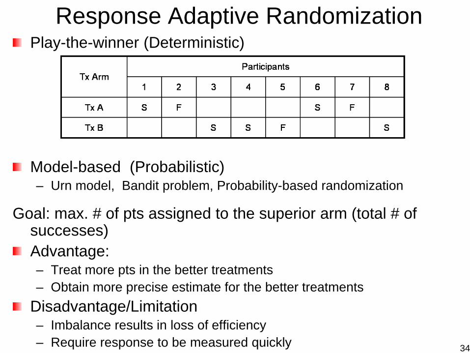
Response Adaptive RandomizationPlay-the-winner (Deterministic)
Model-based (Probabilistic)– Urn model, Bandit problem, Probability-based randomization
Goal: max. # of pts assigned to the superior arm (total # of successes)Advantage:– Treat more pts in the better treatments– Obtain more precise estimate for the better treatments
Disadvantage/Limitation– Imbalance results in loss of efficiency– Require response to be measured quickly 34
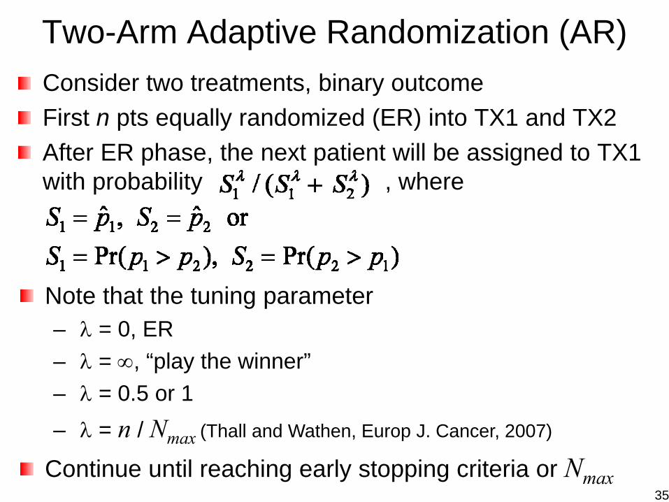
Two-Arm Adaptive Randomization (AR)Consider two treatments, binary outcomeFirst n pts equally randomized (ER) into TX1 and TX2After ER phase, the next patient will be assigned to TX1 with probability , where
Note that the tuning parameter– λ = 0, ER– λ = ∞, “play the winner”– λ = 0.5 or 1– λ = n / Nmax (Thall and Wathen, Europ J. Cancer, 2007)
Continue until reaching early stopping criteria or Nmax35
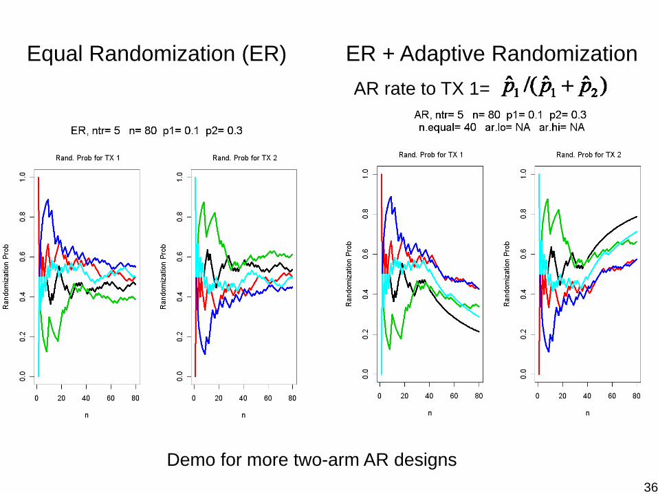
Equal Randomization (ER) ER + Adaptive RandomizationAR rate to TX 1=
Demo for more two-arm AR designs36
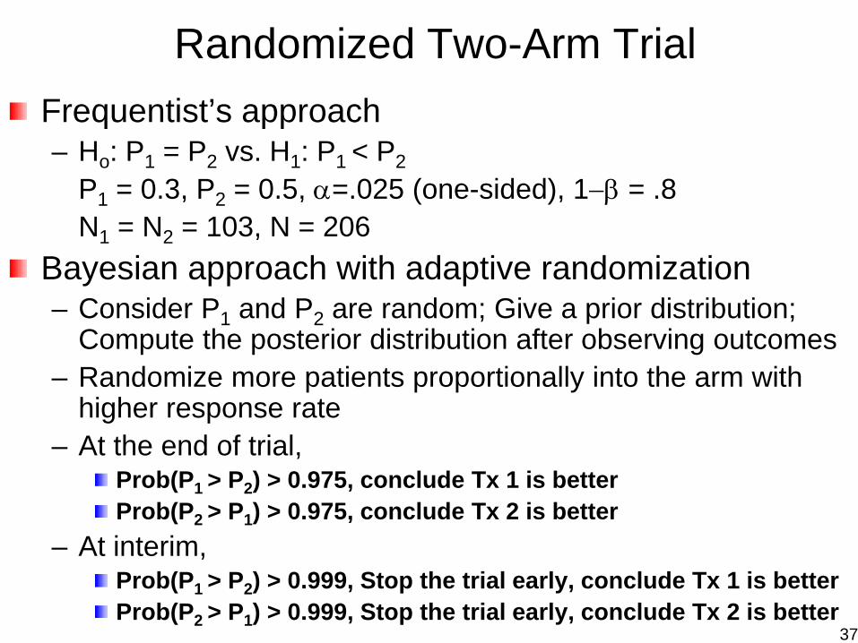
Randomized Two-Arm TrialFrequentist’s approach– Ho: P1 = P2 vs. H1: P1 < P2
P1 = 0.3, P2 = 0.5, α=.025 (one-sided), 1−β = .8N1 = N2 = 103, N = 206
Bayesian approach with adaptive randomization– Consider P1 and P2 are random; Give a prior distribution;
Compute the posterior distribution after observing outcomes– Randomize more patients proportionally into the arm with
higher response rate– At the end of trial,
Prob(P1 > P2) > 0.975, conclude Tx 1 is betterProb(P2 > P1) > 0.975, conclude Tx 2 is better
– At interim,Prob(P1 > P2) > 0.999, Stop the trial early, conclude Tx 1 is betterProb(P2 > P1) > 0.999, Stop the trial early, conclude Tx 2 is better
37
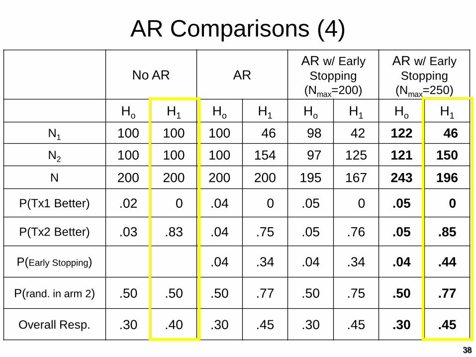
AR Comparisons (4)
No AR ARAR w/ Early
Stopping (Nmax=200)
AR w/ Early Stopping
(Nmax=250)
Ho H1 Ho H1 Ho H1 Ho H1
N1 100 100 100 46 98 42 122 46
N2 100 100 100 154 97 125 121 150
N 200 200 200 200 195 167 243 196
P(Tx1 Better) .02 0 .04 0 .05 0 .05 0
P(Tx2 Better) .03 .83 .04 .75 .05 .76 .05 .85
P(Early Stopping) .04 .34 .04 .34 .04 .44
P(rand. in arm 2) .50 .50 .50 .77 .50 .75 .50 .77
Overall Resp. .30 .40 .30 .45 .30 .45 .30 .45
38
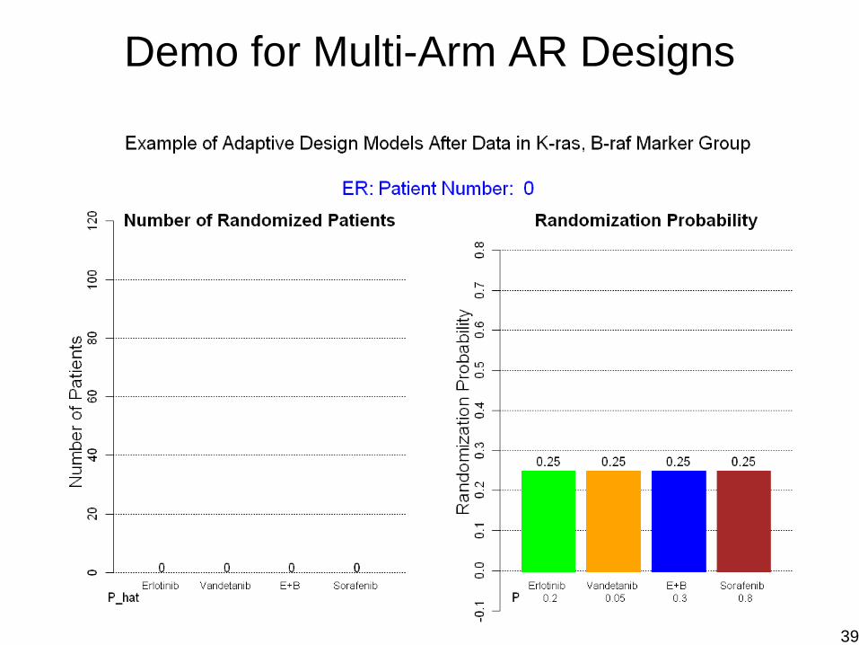
Demo for Multi-Arm AR Designs
39
Biomarker-Based Adaptive DesignsIdentify prognostic and predictive markers for treatments– Prognostic markers
markers that associate with the disease outcome regardless of the treatment: e.g., stage, performance status
– Predictive markersmarkers which predict differential treatment efficacy in different marker groups: e.g., In Marker (−), tx does not workbut in Marker (+), tx works
Test treatment efficacy– Control type I and II error rates– Maximize study power for testing efficacy between txs– Group ethics
Provide better treatment to patients enrolled in the trial– Assign patients into the better treatments with higher probs– Maximize total number of successes in the trial– Individual ethics
40
BATTLE (Biomarker-based Approaches of Targeted Therapy for Lung Cancer
Elimination)
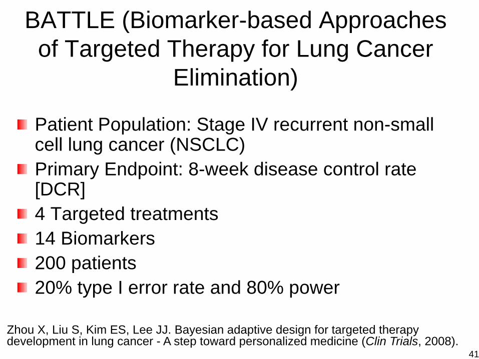
Patient Population: Stage IV recurrent non-small cell lung cancer (NSCLC) Primary Endpoint: 8-week disease control rate [DCR] 4 Targeted treatments14 Biomarkers200 patients20% type I error rate and 80% power
Zhou X, Liu S, Kim ES, Lee JJ. Bayesian adaptive design for targeted therapy development in lung cancer - A step toward personalized medicine (Clin Trials, 2008).
41
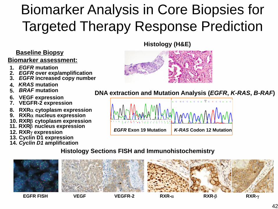
Histology (H&E)
DNA extraction and Mutation Analysis (EGFR, K-RAS, B-RAF)
EGFR Exon 19 Mutation K-RAS Codon 12 Mutation
Histology Sections FISH and Immunohistochemistry
RXR-α RXR-β RXR-γVEGF VEGFR-2
Biomarker Analysis in Core Biopsies for Targeted Therapy Response Prediction
Baseline BiopsyBiomarker assessment:1. EGFR mutation2. EGFR over exp/amplification
4. KRAS mutation5.6. VEGF expression7. VEGFR-2 expression8. RXRα cytoplasm expression
10. RXRβ cytoplasm expression
12. RXRγ expression13. Cyclin D1 expression14. Cyclin D1 amplification
BRAF mutation
EGFR FISH
3. EGFR increased copy number
9. RXRα nucleus expression
11. RXRβ nucleus expression
42
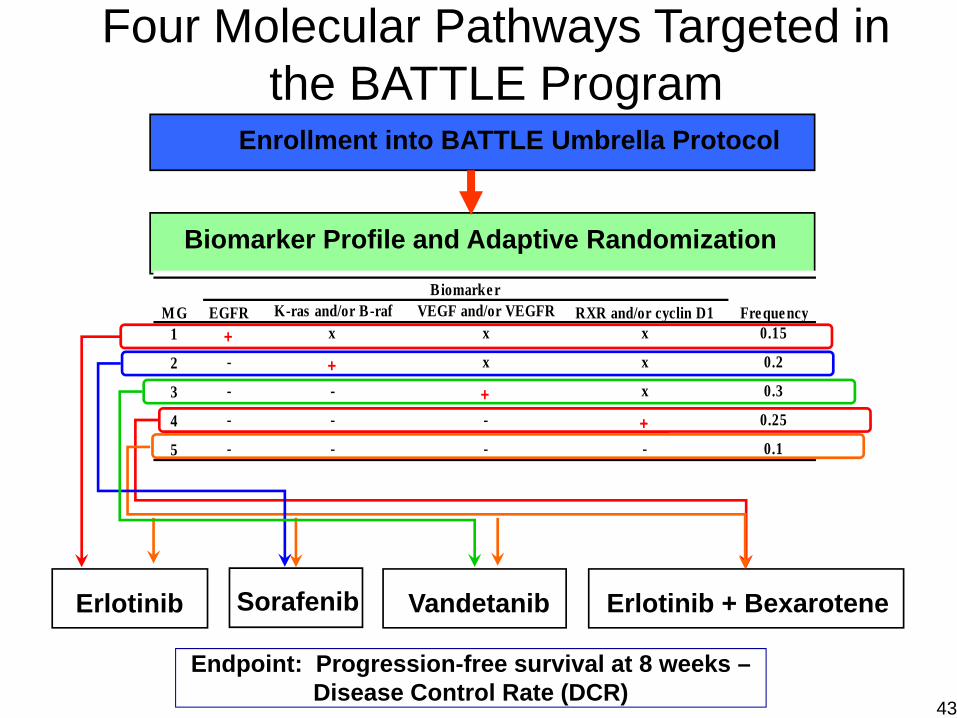
Erlotinib Vandetanib Erlotinib + BexaroteneSorafenib
Biomarker Profile and Adaptive Randomization
Enrollment into BATTLE Umbrella Protocol
Four Molecular Pathways Targeted in the BATTLE Program
Endpoint: Progression-free survival at 8 weeks –Disease Control Rate (DCR)
K-ras and/or B-raf VEGF and/or VEGFR1 + x x x 0.15
2 - + x x 0.2
3 - - + x 0.3
4 - - - + 0.25
5 - - - - 0.1
MGBiomarker
Fre quencyRXR and/or cyclin D1EGFR
43
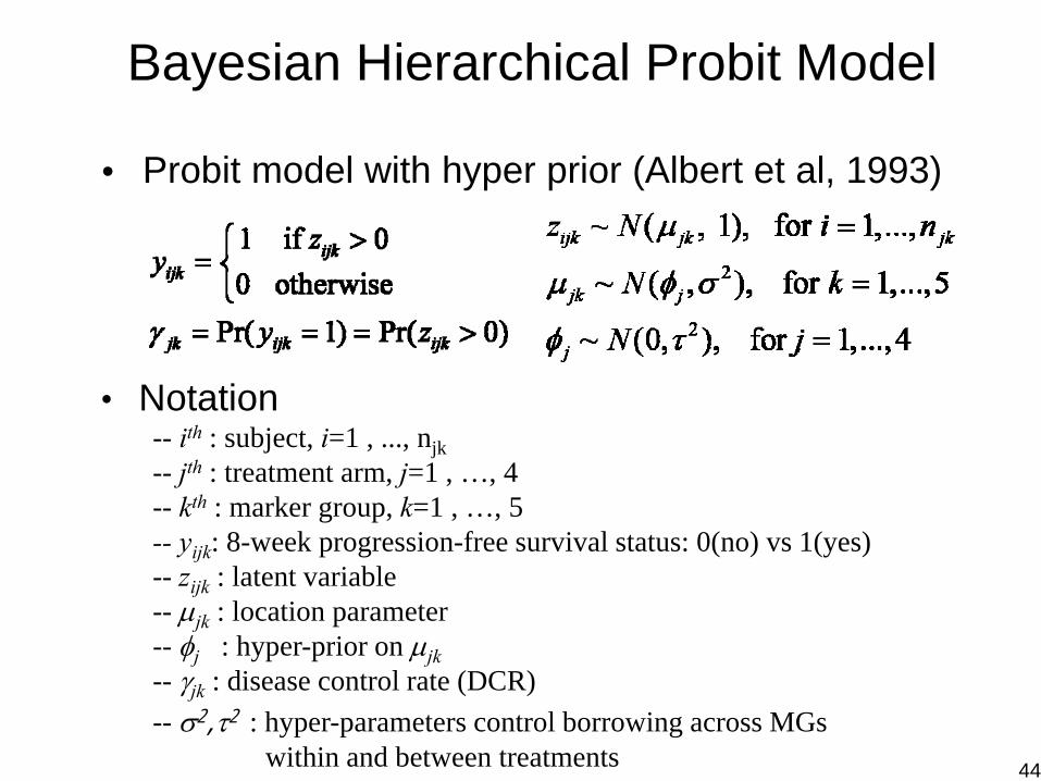
Bayesian Hierarchical Probit Model
• Notation-- ith : subject, i=1 , ..., njk-- jth : treatment arm, j=1 , …, 4-- kth : marker group, k=1 , …, 5-- yijk: 8-week progression-free survival status: 0(no) vs 1(yes)-- zijk : latent variable-- μjk : location parameter-- φj : hyper-prior on μjk-- γjk : disease control rate (DCR)-- σ2,τ2 : hyper-parameters control borrowing across MGs
within and between treatments
• Probit model with hyper prior (Albert et al, 1993)
44
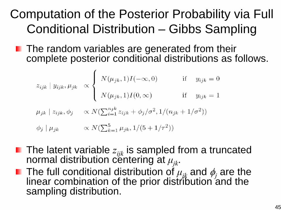
Computation of the Posterior Probability via Full Conditional Distribution – Gibbs SamplingThe random variables are generated from their complete posterior conditional distributions as follows.
The latent variable zijk is sampled from a truncated normal distribution centering at μjk.The full conditional distribution of μjk and φj are the linear combination of the prior distribution and the sampling distribution.
45
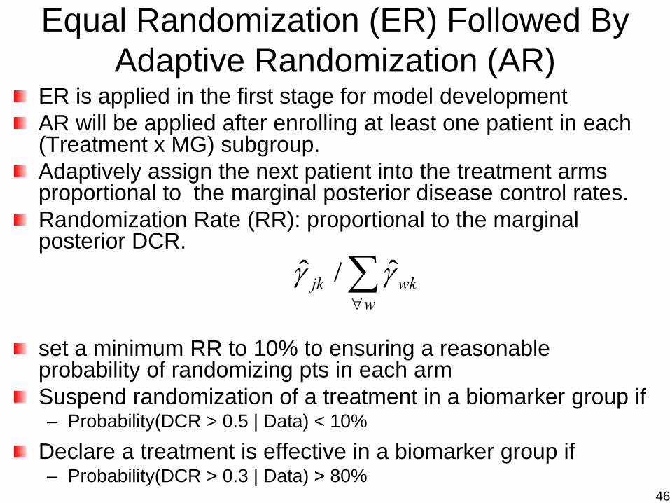
ER is applied in the first stage for model developmentAR will be applied after enrolling at least one patient in each (Treatment x MG) subgroup.Adaptively assign the next patient into the treatment arms proportional to the marginal posterior disease control rates. Randomization Rate (RR): proportional to the marginal posterior DCR.
set a minimum RR to 10% to ensuring a reasonable probability of randomizing pts in each armSuspend randomization of a treatment in a biomarker group if – Probability(DCR > 0.5 | Data) < 10%
Declare a treatment is effective in a biomarker group if – Probability(DCR > 0.3 | Data) > 80%
ˆ ˆ/jk wkw
γ γ∀∑
Equal Randomization (ER) Followed By Adaptive Randomization (AR)
46
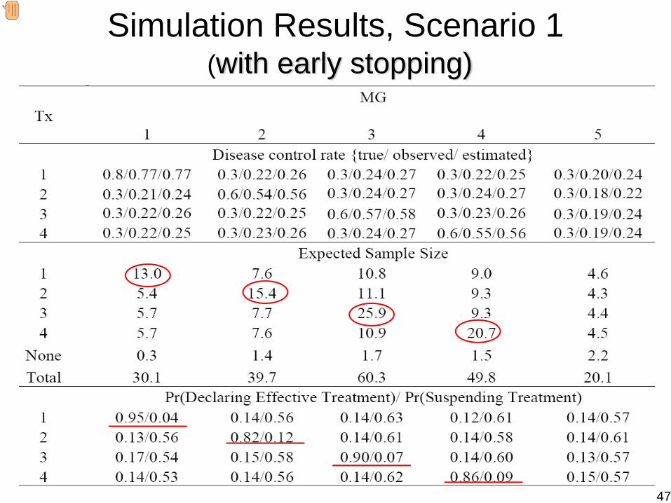
Simulation Results, Scenario 1(with early stopping)
47
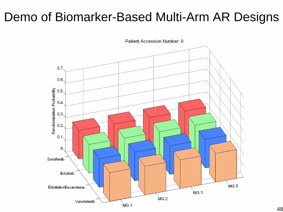
Demo of Biomarker-Based Multi-Arm AR Designs
48
49
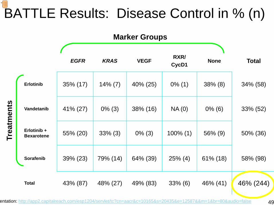
BATTLE Results: Disease Control in % (n)
EGFR KRAS VEGFRXR/
CycD1None Total
Erlotinib 35% (17) 14% (7) 40% (25) 0% (1) 38% (8) 34% (58)
Vandetanib 41% (27) 0% (3) 38% (16) NA (0) 0% (6) 33% (52)
Erlotinib + Bexarotene 55% (20) 33% (3) 0% (3) 100% (1) 56% (9) 50% (36)
Sorafenib 39% (23) 79% (14) 64% (39) 25% (4) 61% (18) 58% (98)
Total 43% (87) 48% (27) 49% (83) 33% (6) 46% (41) 46% (244)
Trea
tmen
ts
Marker Groups
entation: http://app2.capitalreach.com/esp1204/servlet/tc?cn=aacr&c=10165&s=20435&e=12587&&m=1&br=80&audio=false
Lessons Learned from BATTLEBiomarker-based adaptive design is doable! It is well received by clinicians and patients.Prospective tissues collection & biomarkers analysis provide a wealth of informationTreatment effect and predictive markers are efficiently assessed. Pre-selecting markers is not a good idea. We don’t know what are the best predictive markers at get-go.Bundling markers into groups, although can reduce total number of marker patterns, is not the best way to use the marker information either.AR should kicks in early & needs to be closely monitored.AR works well only when we have good drugs and good predictive markers. 50
Section 4.4: Adaptive Randomization“Bayesians don’t need/like randomization”
plays no role in calculating posterior probabilities(whereas crucial for frequentist inference)
we can control for prognosis-related covariates anyway
ethically difficult for physicians
patients willing to be randomized are inherently different
Our take: Randomization IS still essential:
ensures pt prognosis is uncorrelated with trt assigned
balances trt assignment within patient subgroups
we can’t control for unknown/unmeasured covariates!
BUT: Note that we needn’t randomize patients with equalprobabilities to all arms...
Bayesian Adaptive Methods for Clinical Trials – p. 90/100
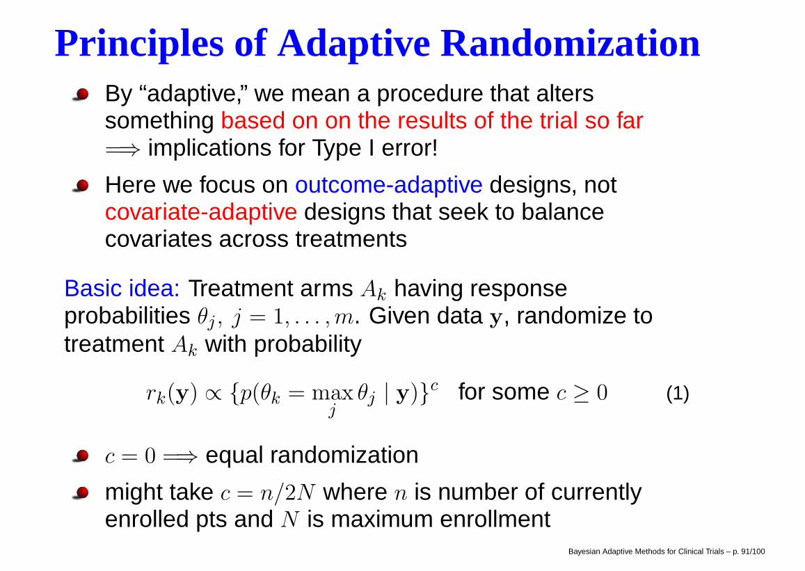
Principles of Adaptive RandomizationBy “adaptive,” we mean a procedure that alterssomething based on on the results of the trial so far=⇒ implications for Type I error!
Here we focus on outcome-adaptive designs, notcovariate-adaptive designs that seek to balancecovariates across treatments
Basic idea: Treatment arms Ak having responseprobabilities θj , j = 1, . . . ,m. Given data y, randomize totreatment Ak with probability
rk(y) ∝ {p(θk = maxj
θj | y)}c for some c ≥ 0 (1)
c = 0 =⇒ equal randomization
might take c = n/2N where n is number of currentlyenrolled pts and N is maximum enrollment
Bayesian Adaptive Methods for Clinical Trials – p. 91/100
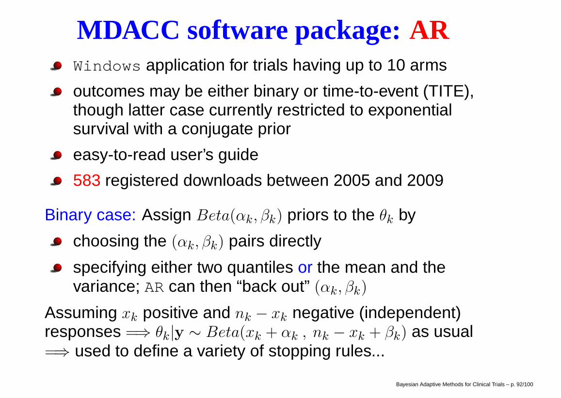
MDACC software package:ARWindows application for trials having up to 10 arms
outcomes may be either binary or time-to-event (TITE),though latter case currently restricted to exponentialsurvival with a conjugate prior
easy-to-read user’s guide
583 registered downloads between 2005 and 2009
Binary case: Assign Beta(αk, βk) priors to the θk by
choosing the (αk, βk) pairs directly
specifying either two quantiles or the mean and thevariance; AR can then “back out” (αk, βk)
Assuming xk positive and nk − xk negative (independent)responses =⇒ θk|y ∼ Beta(xk + αk , nk − xk + βk) as usual=⇒ used to define a variety of stopping rules...
Bayesian Adaptive Methods for Clinical Trials – p. 92/100
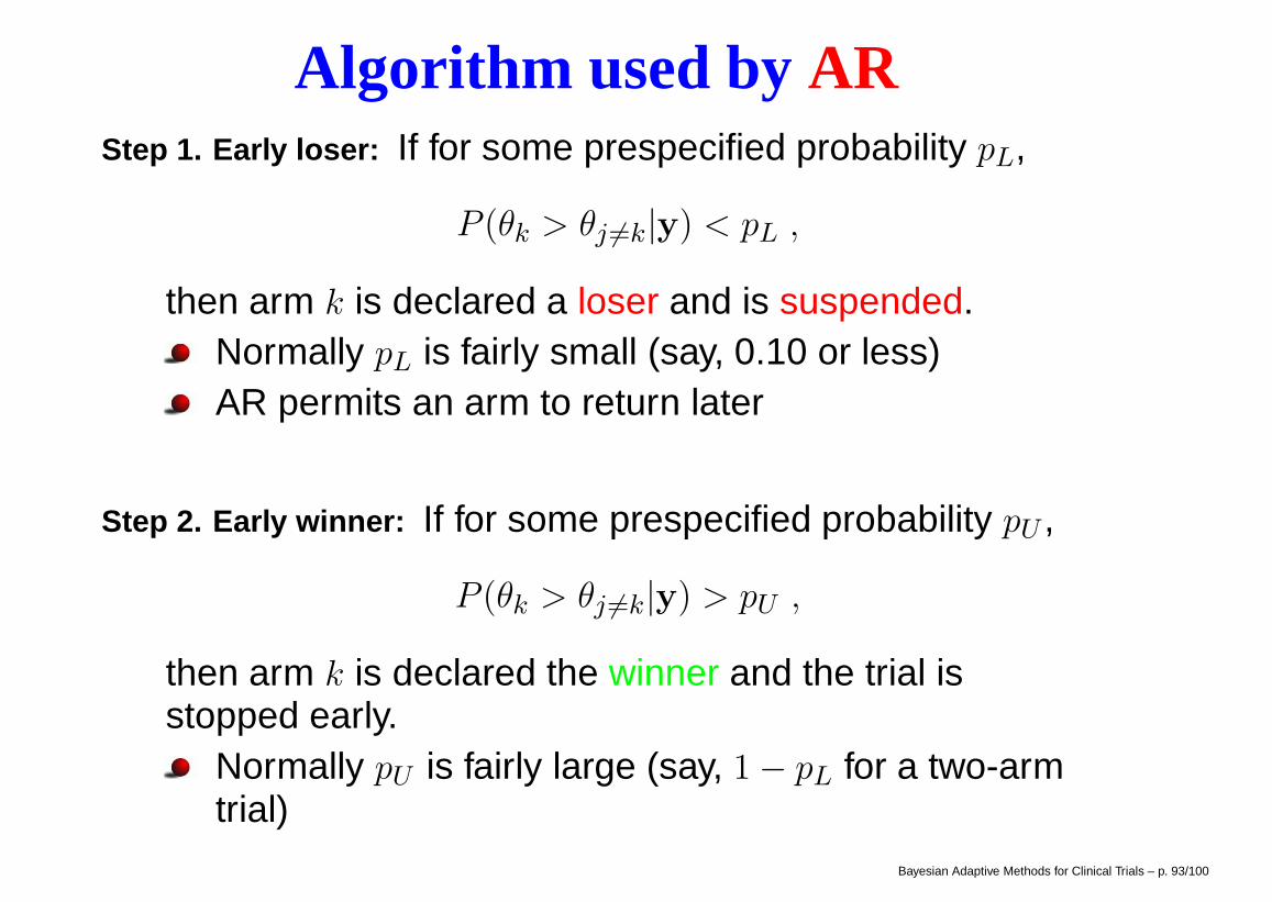
Algorithm used by ARStep 1. Early loser: If for some prespecified probability pL,
P (θk > θj 6=k|y) < pL ,
then arm k is declared a loser and is suspended.Normally pL is fairly small (say, 0.10 or less)AR permits an arm to return later
Step 2. Early winner: If for some prespecified probability pU ,
P (θk > θj 6=k|y) > pU ,
then arm k is declared the winner and the trial isstopped early.
Normally pU is fairly large (say, 1− pL for a two-armtrial)
Bayesian Adaptive Methods for Clinical Trials – p. 93/100
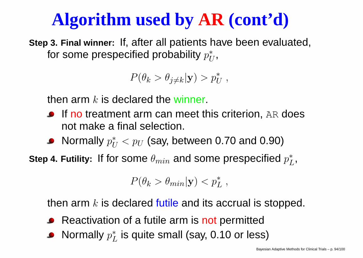
Algorithm used by AR (cont’d)Step 3. Final winner: If, after all patients have been evaluated,
for some prespecified probability p∗U ,
P (θk > θj 6=k|y) > p∗U ,
then arm k is declared the winner.If no treatment arm can meet this criterion, AR doesnot make a final selection.Normally p∗U < pU (say, between 0.70 and 0.90)
Step 4. Futility: If for some θmin and some prespecified p∗L,
P (θk > θmin|y) < p∗L ,
then arm k is declared futile and its accrual is stopped.
Reactivation of a futile arm is not permittedNormally p∗L is quite small (say, 0.10 or less)
Bayesian Adaptive Methods for Clinical Trials – p. 94/100
Example: Sensitizer TrialGoal: Evaluate ability of a “sensitizer” (given concurrentlywith another chemotherapeutic agent) to produce completeremission (CR) at 28 days post-treatment
Classical two-arm comparison of drug-plus-sensitizervs. drug alone ⇒ sample size near 100 – too large forour accrual rate of just 30/year!
Instead, use some prior information with a Bayesian ARdesign having
maximum patient accrual = 60
minimum randomization probability = 0.10
first 14 patients randomized fairly (7 to each arm)before AR begins
AR tuning parameter c = 1 (i.e., modest deviation fromequal randomization after the first 14 patients)
Bayesian Adaptive Methods for Clinical Trials – p. 95/100
Priors for the Sensitizer Trial
0.0 0.2 0.4 0.6 0.8 1.0
01
23
45
6
θ
density
Arm 1 (control)
Arm 2 (sensitizer)
0.0 0.2 0.4 0.6 0.8 1.0
01
23
45
6
θdensity
Arm 1 (control)
Arm 2 (sensitizer)
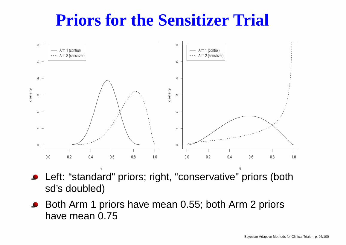
Left: “standard" priors; right, “conservative" priors (bothsd’s doubled)
Both Arm 1 priors have mean 0.55; both Arm 2 priorshave mean 0.75
Bayesian Adaptive Methods for Clinical Trials – p. 96/100
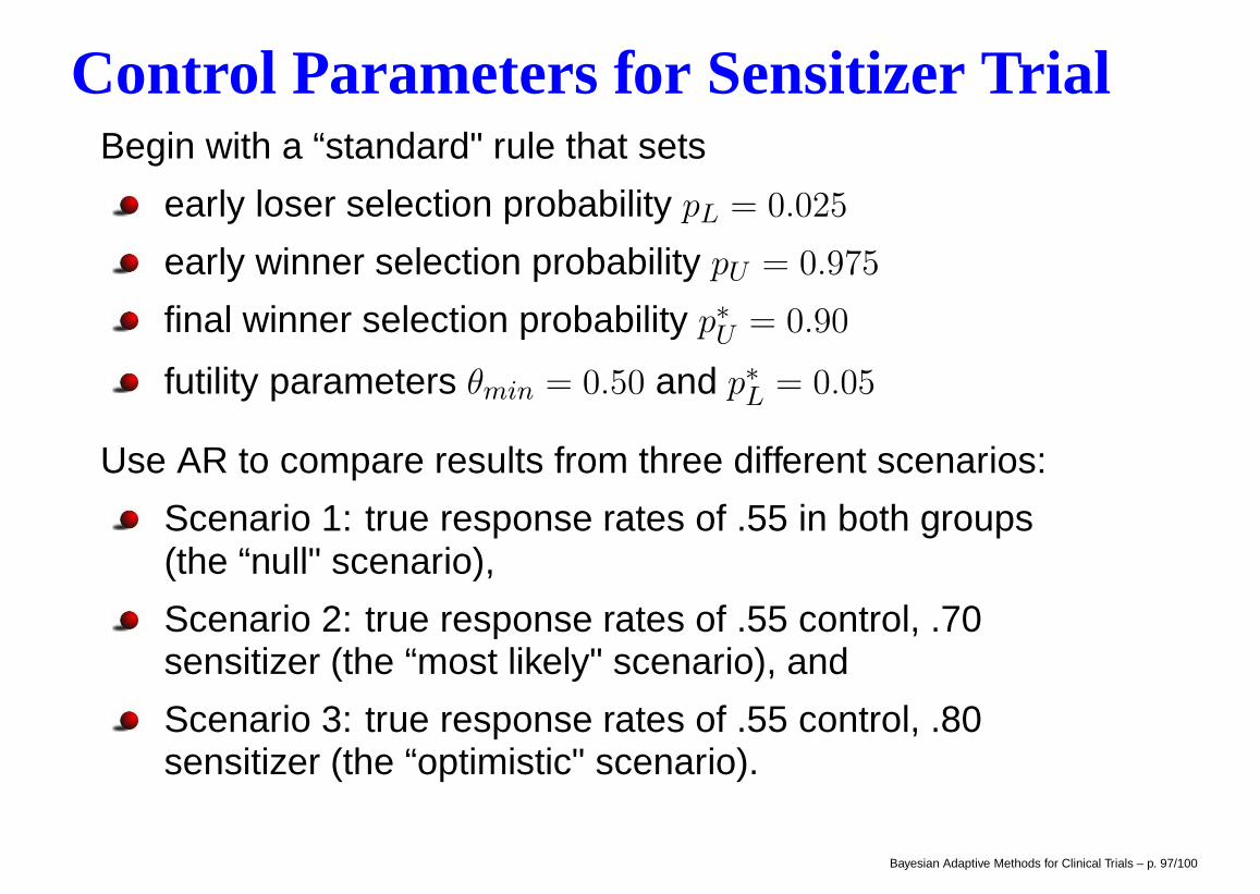
Control Parameters for Sensitizer TrialBegin with a “standard" rule that sets
early loser selection probability pL = 0.025
early winner selection probability pU = 0.975
final winner selection probability p∗U = 0.90
futility parameters θmin = 0.50 and p∗L = 0.05
Use AR to compare results from three different scenarios:
Scenario 1: true response rates of .55 in both groups(the “null" scenario),
Scenario 2: true response rates of .55 control, .70sensitizer (the “most likely" scenario), and
Scenario 3: true response rates of .55 control, .80sensitizer (the “optimistic" scenario).
Bayesian Adaptive Methods for Clinical Trials – p. 97/100
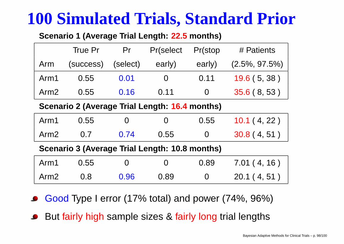
100 Simulated Trials, Standard PriorScenario 1 (Average Trial Length: 22.5 months)
True Pr Pr Pr(select Pr(stop # Patients
Arm (success) (select) early) early) (2.5%, 97.5%)
Arm1 0.55 0.01 0 0.11 19.6 ( 5, 38 )
Arm2 0.55 0.16 0.11 0 35.6 ( 8, 53 )
Scenario 2 (Average Trial Length: 16.4 months)
Arm1 0.55 0 0 0.55 10.1 ( 4, 22 )
Arm2 0.7 0.74 0.55 0 30.8 ( 4, 51 )
Scenario 3 (Average Trial Length: 10.8 months)
Arm1 0.55 0 0 0.89 7.01 ( 4, 16 )
Arm2 0.8 0.96 0.89 0 20.1 ( 4, 51 )
Good Type I error (17% total) and power (74%, 96%)
But fairly high sample sizes & fairly long trial lengths
Bayesian Adaptive Methods for Clinical Trials – p. 98/100
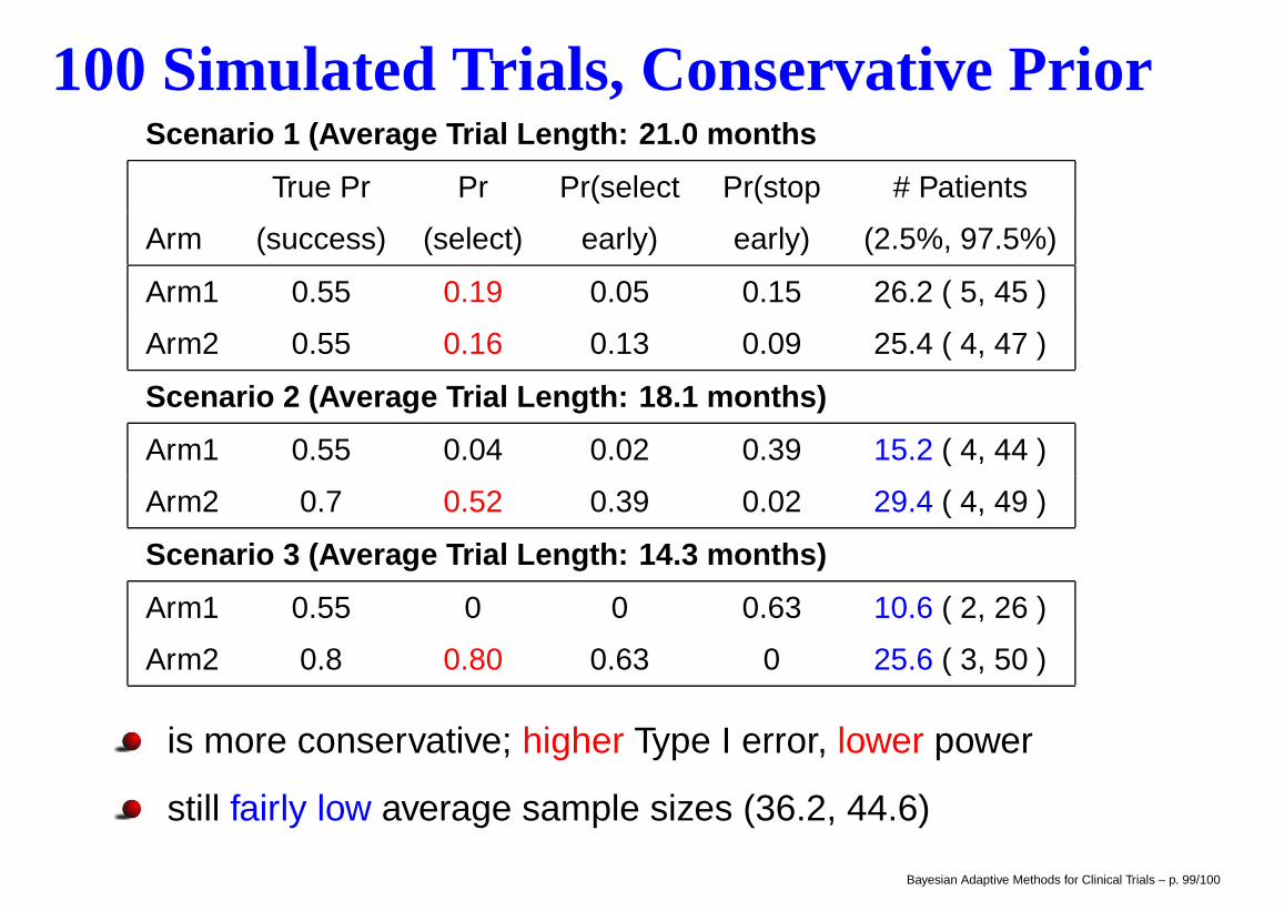
100 Simulated Trials, Conservative PriorScenario 1 (Average Trial Length: 21.0 months
True Pr Pr Pr(select Pr(stop # Patients
Arm (success) (select) early) early) (2.5%, 97.5%)
Arm1 0.55 0.19 0.05 0.15 26.2 ( 5, 45 )
Arm2 0.55 0.16 0.13 0.09 25.4 ( 4, 47 )
Scenario 2 (Average Trial Length: 18.1 months)
Arm1 0.55 0.04 0.02 0.39 15.2 ( 4, 44 )
Arm2 0.7 0.52 0.39 0.02 29.4 ( 4, 49 )
Scenario 3 (Average Trial Length: 14.3 months)
Arm1 0.55 0 0 0.63 10.6 ( 2, 26 )
Arm2 0.8 0.80 0.63 0 25.6 ( 3, 50 )
is more conservative; higher Type I error, lower power
still fairly low average sample sizes (36.2, 44.6)
Bayesian Adaptive Methods for Clinical Trials – p. 99/100
Summary
MD Anderson software available athttps://biostatistics.mdanderson.org/SoftwareDownload/
BCLM text-related software available at:http://www.biostat.umn.edu/∼brad/data3.html
BRugs package installation and further examples:http://www.biostat.umn.edu/∼brad/software/BRugs/
Related design site for binary and Cox PH models:www.biostat.umn.edu/∼brianho/papers/2007/JBS/prac_bayes_design.html
Thanks for your attention!
Bayesian Adaptive Methods for Clinical Trials – p. 100/100
Intro Power Priors Alternatives Metaanalysis GLMs Rando Discussion
Hierarchical Commensurate Prior Modelsfor Adaptive Incorporation of
Historical Information in Clinical Trials
Brian P. Hobbs1, Bradley P. Carlin2,Sumithra Mandrekar,3 and Daniel Sargent3
1 Department of Biostatistics, University of Texas M.D. Anderson Cancer Center,Houston, TX
2 Division of Biostatistics, School of Public Health, University of Minnesota,Minneapolis, MN
3 Mayo Clinic, Rochester, MN
University of Chicago, Department of Health Studies,December 7, 2011

Intro Power Priors Alternatives Metaanalysis GLMs Rando DiscussionBackground
Using Historical Data
I Email 8 Sep 2008 from Dr. Telba Irony, FDA: “When we tryto borrow strength from only one historical study (be it acontrol group or a treatment group) ... [the results] becomeVERY sensitive to the hyperprior [on the variance parametersthat control the amount of borrowing].”
I Borrowing from historical data offers advantages:I reduced sample size (at least in control group) hence lower
cost and ethical hazard, plus higher power
but also disadvantages:I higher Type I error, plus a possibly lengthier trial if the
informative prior turns out to be wrong
I Thus what is needed is a recipe for how much strength toborrow from the historical data
I One possibility: “back out” this amount based on Type I errorand power considerations. This is often done, but tends todefeat the historical data’s original purpose!

Intro Power Priors Alternatives Metaanalysis GLMs Rando DiscussionIntro Commensurate Power Priors Linear Model Example
Proposed Solution: Power Priors
I Introduced by Ibrahim and Chen (2000, Statistical Science)
I Let D0 = (n0, x0) denote historical data, suppose θ is theparameter of interest, and let L(D0|θ) denote the generallikelihood
I Suppose π0(θ) is the prior distribution on θ before D0 isobserved, the initial prior
I The conditional power prior on θ for the current study is thehistorical likelihood, L(D0|θ), raised to power α0, whereα0 ∈ [0, 1], multiplied by the initial prior:
π(θ|D0, α0) ∝ L(D0|θ)α0π0(θ) ,
I α0 is the power parameter that controls the “degree ofborrowing” from D0
Intro Power Priors Alternatives Metaanalysis GLMs Rando DiscussionIntro Commensurate Power Priors Linear Model Example
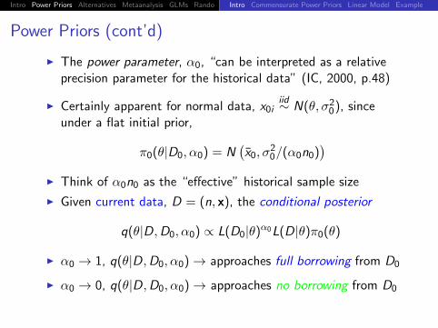
Power Priors (cont’d)
I The power parameter, α0, “can be interpreted as a relativeprecision parameter for the historical data” (IC, 2000, p.48)
I Certainly apparent for normal data, x0iiid∼ N(θ, σ20), since
under a flat initial prior,
π0(θ|D0, α0) = N(x0, σ
20/(α0n0)
)I Think of α0n0 as the “effective” historical sample size
I Given current data, D = (n, x), the conditional posterior
q(θ|D,D0, α0) ∝ L(D0|θ)α0L(D|θ)π0(θ)
I α0 → 1, q(θ|D,D0, α0)→ approaches full borrowing from D0
I α0 → 0, q(θ|D,D0, α0)→ approaches no borrowing from D0

Intro Power Priors Alternatives Metaanalysis GLMs Rando DiscussionIntro Commensurate Power Priors Linear Model Example
Power Priors (cont’d)
I We could fix α0 ∈ [0, 1] and assume consistency among D0
and D is known, but if this is not the case, models with poorfrequentist operating characteristics may result
I Choosing a hyperprior, π(α0), for α0 enables the data to helpdetermine probable values for α0
I Ibrahim-Chen (2000) propose joint power priors of form
π(θ, α0|D0) ∝ L(D0|θ)α0π0(θ)π(α0)
I Duan et al. (2006), Neuenschwander et al. (2009), andPericchi (2009) propose modified joint power priors (MPP)which respect the Likelihood Principle,
π(θ, α0|D0) ∝ L(D0|θ)α0π0(θ)∫L(D0|θ)α0π0(θ)dθ
π(α0)
Intro Power Priors Alternatives Metaanalysis GLMs Rando DiscussionIntro Commensurate Power Priors Linear Model Example
Location Commensurate Power Priors (LCPP)
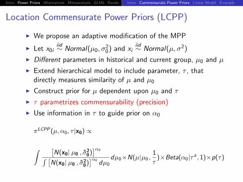
I We propose an adaptive modification of the MPP
I Let x0iiid∼ Normal(µ0, σ
20) and xi
iid∼ Normal(µ, σ2)
I Different parameters in historical and current group, µ0 and µ
I Extend hierarchical model to include parameter, τ , thatdirectly measures similarity of µ and µ0
I Construct prior for µ dependent upon µ0 and τ
I τ parametrizes commensurability (precision)
I Use information in τ to guide prior on α0
πLCPP(µ, α0, τ |x0) ∝
∫ [N(x0| µ0 , σ
20)]α0∫ [
N(x0| µ0 , σ20)]α0 dµ0
dµ0×N(µ|µ0 ,1
τ)×Beta(α0|τ a , 1)×p(τ)
Intro Power Priors Alternatives Metaanalysis GLMs Rando DiscussionIntro Commensurate Power Priors Linear Model Example
LCPP for Single Arm Trial
I Formalize commensurate as µ0 near µ by adopting Normalprior on µ with mean µ0 and precision τ
I Beta(τ a , 1) prior on α0 for some a > 0
I τ close to 0 corresponds to very low commensurability, whilevery large τ implies the two datasets may arise from similarpopulations
I τ →∞, point-mass prior on α0 at 1
I τ → 0 discourages incorporation of historical information
I Requires a fixed, known sampling historical variance σ20 (MLE)
Intro Power Priors Alternatives Metaanalysis GLMs Rando DiscussionIntro Commensurate Power Priors Linear Model Example
LCPP for Single Arm Trial (cont’d)
I Both α0 and τ inflate the “prior” variance
πLCPP(µ, α0, τ |x0) ∝ N(µ| x0 ,1
τ+
σ20
α0n0)× Beta(α0|τ a , 1)× p(τ)
I Prior on τ : Mixture of two gammas with mixing probabilityω = 1/2 and with hyperparameter a = 1/2 provides sufficientflexibility:
p(τ) ∝(ωGamma(τ | 1 , 10) + (1− ω)Gamma(τ | 3/2 ,
1
1000)
)
I Posterior obtained after multiplying by current likelihoodN(x| µ , σ2) and vague (say reference) prior on σ2
I q(σ2|x) ∝ IG(n2 ,
n2
[s2 + (x − µ)2
])
Intro Power Priors Alternatives Metaanalysis GLMs Rando DiscussionIntro Commensurate Power Priors Linear Model Example
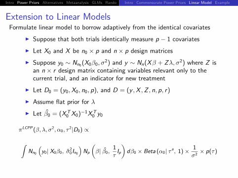
Extension to Linear ModelsFormulate linear model to borrow adaptively from the identical covariates
I Suppose that both trials identically measure p − 1 covariates
I Let X0 and X be n0 × p and n × p design matrices
I Suppose y0 ∼ Nn0(X0β0, σ2) and y ∼ Nn(Xβ + Zλ, σ2) where Z is
an n × r design matrix containing variables relevant only to thecurrent trial, and an indicator for new treatment
I Let D0 = (y0,X0, n0, p), and D = (y ,X ,Z , n, p, r)
I Assume flat prior for λ
I Let β0 = (XT0 X0)−1XT
0 y0
πLCPP(β, λ, σ2, α0, τ2|D0) ∝
∫Nn0
(y0| X0β0, σ
20 In0
)Np
(β| β0,
1
τIp
)dβ0 × Beta (α0| τ a, 1)× 1
σ2× p(τ)
Intro Power Priors Alternatives Metaanalysis GLMs Rando DiscussionIntro Commensurate Power Priors Linear Model Example
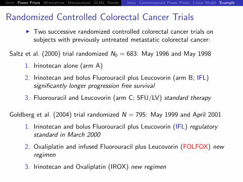
Randomized Controlled Colorectal Cancer Trials
I Two successive randomized controlled colorectal cancer trials onsubjects with previously untreated metastatic colorectal cancer:
Saltz et al. (2000) trial randomized N0 = 683: May 1996 and May 1998
1. Irinotecan alone (arm A)
2. Irinotecan and bolus Fluorouracil plus Leucovorin (arm B; IFL)significantly longer progression free survival
3. Fluorouracil and Leucovorin (arm C; 5FU/LV) standard therapy
Goldberg et al. (2004) trial randomized N = 795: May 1999 and April 2001
1. Irinotecan and bolus Fluorouracil plus Leucovorin (IFL) regulatorystandard in March 2000
2. Oxaliplatin and infused Fluorouracil plus Leucovorin (FOLFOX) newregimen
3. Irinotecan and Oxaliplatin (IROX) new regimen
Intro Power Priors Alternatives Metaanalysis GLMs Rando DiscussionIntro Commensurate Power Priors Linear Model Example
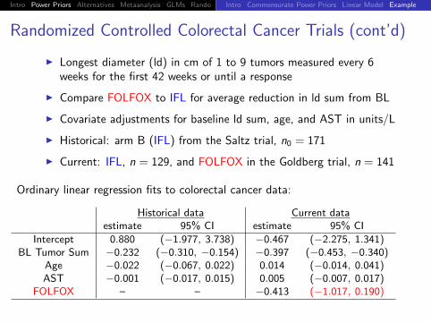
Randomized Controlled Colorectal Cancer Trials (cont’d)
I Longest diameter (ld) in cm of 1 to 9 tumors measured every 6weeks for the first 42 weeks or until a response
I Compare FOLFOX to IFL for average reduction in ld sum from BL
I Covariate adjustments for baseline ld sum, age, and AST in units/L
I Historical: arm B (IFL) from the Saltz trial, n0 = 171
I Current: IFL, n = 129, and FOLFOX in the Goldberg trial, n = 141
Ordinary linear regression fits to colorectal cancer data:
Historical data Current dataestimate 95% CI estimate 95% CI
Intercept 0.880 (−1.977, 3.738) −0.467 (−2.275, 1.341)BL Tumor Sum −0.232 (−0.310, −0.154) −0.397 (−0.453, −0.340)
Age −0.022 (−0.067, 0.022) 0.014 (−0.014, 0.041)AST −0.001 (−0.017, 0.015) 0.005 (−0.007, 0.017)
FOLFOX – – −0.413 (−1.017, 0.190)
Intro Power Priors Alternatives Metaanalysis GLMs Rando DiscussionIntro Commensurate Power Priors Linear Model Example
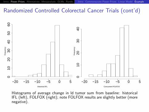
Randomized Controlled Colorectal Cancer Trials (cont’d)
Historical IFL
Fre
quen
cy
−20 −15 −10 −5 0 5
010
2030
4050
60
Concurrent FOLFOX
Fre
quen
cy
−20 −15 −10 −5 0 50
1020
3040
Histograms of average change in ld tumor sum from baseline: historicalIFL (left), FOLFOX (right); note FOLFOX results are slightly better (morenegative).
Intro Power Priors Alternatives Metaanalysis GLMs Rando DiscussionIntro Commensurate Power Priors Linear Model Example
Randomized Controlled Colorectal Cancer Trial (cont’d)
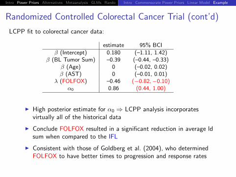
LCPP fit to colorectal cancer data:
estimate 95% BCI
β (Intercept) 0.180 (–1.11, 1.42)β (BL Tumor Sum) –0.39 (–0.44, –0.33)
β (Age) 0 (–0.02, 0.02)β (AST) 0 (–0.01, 0.01)
λ (FOLFOX) –0.46 (−0.82,−0.10)α0 0.86 (0.44, 1.00)
I High posterior estimate for α0 ⇒ LCPP analysis incorporatesvirtually all of the historical data
I Conclude FOLFOX resulted in a significant reduction in average ldsum when compared to the IFL
I Consistent with those of Goldberg et al. (2004), who determinedFOLFOX to have better times to progression and response rates

Intro Power Priors Alternatives Metaanalysis GLMs Rando DiscussionEqual Sampling Variances Unequal Sampling Variances
Competing Non-Power Prior Approaches
Let x0iiid∼ Normal(µ0, σ
20) and xi
iid∼ Normal(µ, σ2)
1. Cauchy prior on µ centered at historical sample mean x0I πcau ∝ Cauchy(µ|median = x0, scale = γ)
2. Location Commensurate Prior (LCP)I Adaptive mechanism based solely on the commensurability
parameter τ :
πLCP(µ, σ2, τ |x0) ∝ N(µ| x0 ,1
τ+σ20
n0)× 1
σ2× p(τ)
I We use a mixture prior on τ , often with ω = 1/2:
p(τ) ∝(ωGamma(τ | 1 , 10) + (1− ω)Gamma(τ | 3/2 ,
1
1000)
)
Intro Power Priors Alternatives Metaanalysis GLMs Rando DiscussionEqual Sampling Variances Unequal Sampling Variances
Non-Power Prior Approaches (cont’d)
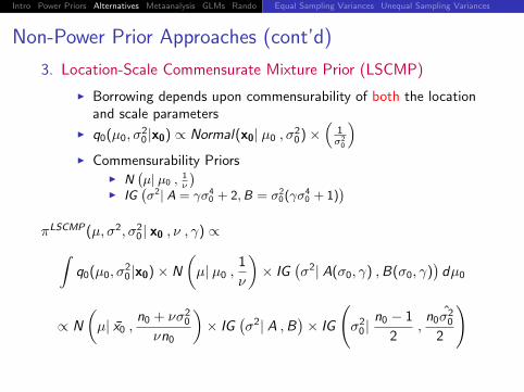
3. Location-Scale Commensurate Mixture Prior (LSCMP)
I Borrowing depends upon commensurability of both the locationand scale parameters
I q0(µ0, σ20 |x0) ∝ Normal(x0| µ0 , σ
20)×
(1σ20
)I Commensurability Priors
I N(µ| µ0 ,
1ν
)I IG
(σ2| A = γσ4
0 + 2,B = σ20(γσ4
0 + 1))
πLSCMP(µ, σ2, σ20 | x0 , ν , γ) ∝∫
q0(µ0, σ20 |x0)× N
(µ| µ0 ,
1
ν
)× IG
(σ2| A(σ0, γ) ,B(σ0, γ)
)dµ0
∝ N
(µ| x0 ,
n0 + νσ20
νn0
)× IG
(σ2| A ,B
)× IG
(σ20 |
n0 − 1
2,
n0σ20
2
)

Intro Power Priors Alternatives Metaanalysis GLMs Rando DiscussionEqual Sampling Variances Unequal Sampling Variances
Non-Power Prior Approaches (cont’d)
3. Location-Scale Commensurate Mixture Prior (cont’d)
I Fix values of ν = (ν1, ν0) and γ = (γ1, γ0) corresponding to highand low precision
I ν = (1012, (10σ20)−1)
I γ = (102, 5−1)
I Formulate mixture prior with fixed mixing probability θ such thatπ?(µ, σ|x0, ν, γ, θ) is proportional to
θπ(µ, σ2, σ20| x0 , ν1 , γ1) + (1− θ)π(µ, σ2, σ20| x0 , ν0 , γ0) ,
where fixing θ = 0.5 seems to work well.
Intro Power Priors Alternatives Metaanalysis GLMs Rando DiscussionEqual Sampling Variances Unequal Sampling Variances
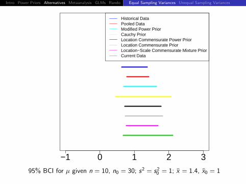
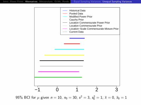
−1 0 1 2 3
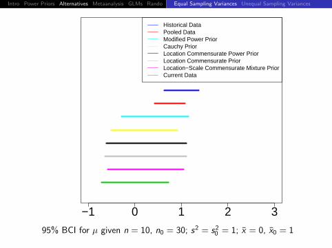
Historical DataPooled DataModified Power PriorCauchy PriorLocation Commensurate Power PriorLocation Commensurate PriorLocation−Scale Commensurate Mixture PriorCurrent Data
95% BCI for µ given n = 10, n0 = 30; s2 = s20 = 1; x = 0, x0 = 1

Intro Power Priors Alternatives Metaanalysis GLMs Rando DiscussionEqual Sampling Variances Unequal Sampling Variances
−1 0 1 2 3
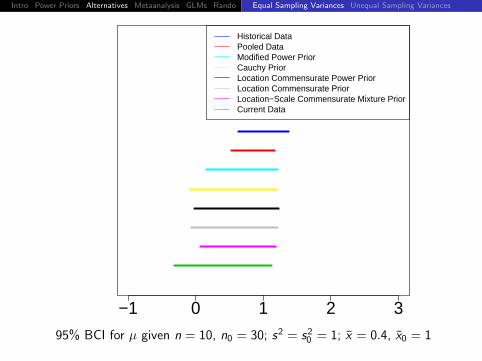
Historical DataPooled DataModified Power PriorCauchy PriorLocation Commensurate Power PriorLocation Commensurate PriorLocation−Scale Commensurate Mixture PriorCurrent Data
95% BCI for µ given n = 10, n0 = 30; s2 = s20 = 1; x = 0.2, x0 = 1
Intro Power Priors Alternatives Metaanalysis GLMs Rando DiscussionEqual Sampling Variances Unequal Sampling Variances
−1 0 1 2 3
Historical DataPooled DataModified Power PriorCauchy PriorLocation Commensurate Power PriorLocation Commensurate PriorLocation−Scale Commensurate Mixture PriorCurrent Data
95% BCI for µ given n = 10, n0 = 30; s2 = s20 = 1; x = 0.4, x0 = 1
Intro Power Priors Alternatives Metaanalysis GLMs Rando DiscussionEqual Sampling Variances Unequal Sampling Variances
−1 0 1 2 3
Historical DataPooled DataModified Power PriorCauchy PriorLocation Commensurate Power PriorLocation Commensurate PriorLocation−Scale Commensurate Mixture PriorCurrent Data
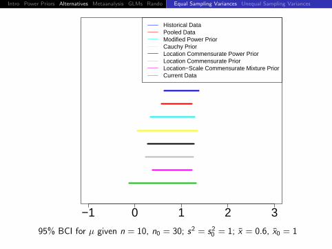
95% BCI for µ given n = 10, n0 = 30; s2 = s20 = 1; x = 0.6, x0 = 1
Intro Power Priors Alternatives Metaanalysis GLMs Rando DiscussionEqual Sampling Variances Unequal Sampling Variances
−1 0 1 2 3
Historical DataPooled DataModified Power PriorCauchy PriorLocation Commensurate Power PriorLocation Commensurate PriorLocation−Scale Commensurate Mixture PriorCurrent Data
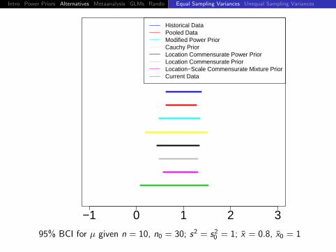
95% BCI for µ given n = 10, n0 = 30; s2 = s20 = 1; x = 0.8, x0 = 1
Intro Power Priors Alternatives Metaanalysis GLMs Rando DiscussionEqual Sampling Variances Unequal Sampling Variances
−1 0 1 2 3
Historical DataPooled DataModified Power PriorCauchy PriorLocation Commensurate Power PriorLocation Commensurate PriorLocation−Scale Commensurate Mixture PriorCurrent Data
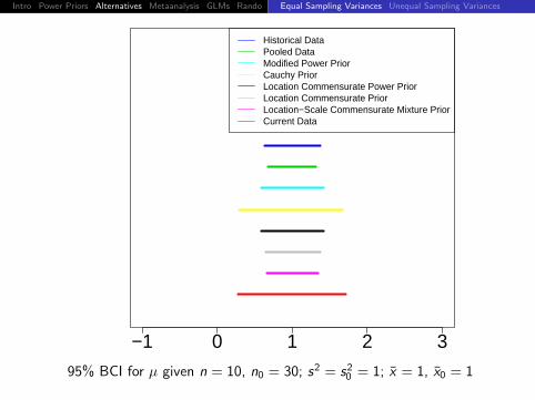
95% BCI for µ given n = 10, n0 = 30; s2 = s20 = 1; x = 1, x0 = 1
Intro Power Priors Alternatives Metaanalysis GLMs Rando DiscussionEqual Sampling Variances Unequal Sampling Variances
−1 0 1 2 3
Historical DataPooled DataModified Power PriorCauchy PriorLocation Commensurate Power PriorLocation Commensurate PriorLocation−Scale Commensurate Mixture PriorCurrent Data
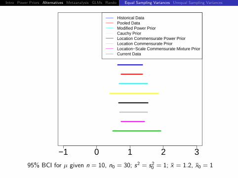
95% BCI for µ given n = 10, n0 = 30; s2 = s20 = 1; x = 1.2, x0 = 1
Intro Power Priors Alternatives Metaanalysis GLMs Rando DiscussionEqual Sampling Variances Unequal Sampling Variances
−1 0 1 2 3
Historical DataPooled DataModified Power PriorCauchy PriorLocation Commensurate Power PriorLocation Commensurate PriorLocation−Scale Commensurate Mixture PriorCurrent Data
95% BCI for µ given n = 10, n0 = 30; s2 = s20 = 1; x = 1.4, x0 = 1
Intro Power Priors Alternatives Metaanalysis GLMs Rando DiscussionEqual Sampling Variances Unequal Sampling Variances
−1 0 1 2 3
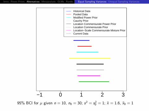
Historical DataPooled DataModified Power PriorCauchy PriorLocation Commensurate Power PriorLocation Commensurate PriorLocation−Scale Commensurate Mixture PriorCurrent Data
95% BCI for µ given n = 10, n0 = 30; s2 = s20 = 1; x = 1.6, x0 = 1
Intro Power Priors Alternatives Metaanalysis GLMs Rando DiscussionEqual Sampling Variances Unequal Sampling Variances
−1 0 1 2 3
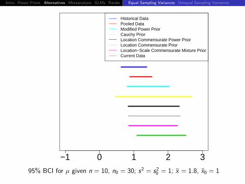
Historical DataPooled DataModified Power PriorCauchy PriorLocation Commensurate Power PriorLocation Commensurate PriorLocation−Scale Commensurate Mixture PriorCurrent Data
95% BCI for µ given n = 10, n0 = 30; s2 = s20 = 1; x = 1.8, x0 = 1
Intro Power Priors Alternatives Metaanalysis GLMs Rando DiscussionEqual Sampling Variances Unequal Sampling Variances
−1 0 1 2 3
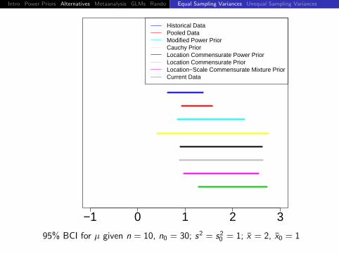
Historical DataPooled DataModified Power PriorCauchy PriorLocation Commensurate Power PriorLocation Commensurate PriorLocation−Scale Commensurate Mixture PriorCurrent Data
95% BCI for µ given n = 10, n0 = 30; s2 = s20 = 1; x = 2, x0 = 1
Intro Power Priors Alternatives Metaanalysis GLMs Rando DiscussionEqual Sampling Variances Unequal Sampling Variances
−1 0 1 2 3
Historical DataPooled DataModified Power PriorCauchy PriorLocation Commensurate Power PriorLocation Commensurate PriorLocation−Scale Commensurate Mixture PriorCurrent Data
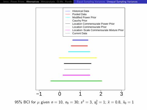
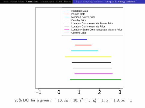
95% BCI for µ given n = 10, n0 = 30; s2 = 3, s20 = 1; x = 0, x0 = 1
Intro Power Priors Alternatives Metaanalysis GLMs Rando DiscussionEqual Sampling Variances Unequal Sampling Variances
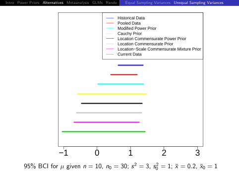
−1 0 1 2 3
Historical DataPooled DataModified Power PriorCauchy PriorLocation Commensurate Power PriorLocation Commensurate PriorLocation−Scale Commensurate Mixture PriorCurrent Data
95% BCI for µ given n = 10, n0 = 30; s2 = 3, s20 = 1; x = 0.2, x0 = 1
Intro Power Priors Alternatives Metaanalysis GLMs Rando DiscussionEqual Sampling Variances Unequal Sampling Variances
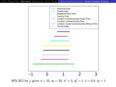
−1 0 1 2 3
Historical DataPooled DataModified Power PriorCauchy PriorLocation Commensurate Power PriorLocation Commensurate PriorLocation−Scale Commensurate Mixture PriorCurrent Data
95% BCI for µ given n = 10, n0 = 30; s2 = 3, s20 = 1; x = 0.4, x0 = 1
Intro Power Priors Alternatives Metaanalysis GLMs Rando DiscussionEqual Sampling Variances Unequal Sampling Variances
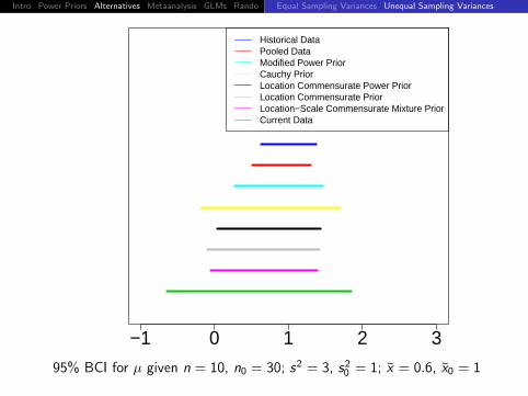
−1 0 1 2 3
Historical DataPooled DataModified Power PriorCauchy PriorLocation Commensurate Power PriorLocation Commensurate PriorLocation−Scale Commensurate Mixture PriorCurrent Data
95% BCI for µ given n = 10, n0 = 30; s2 = 3, s20 = 1; x = 0.6, x0 = 1
Intro Power Priors Alternatives Metaanalysis GLMs Rando DiscussionEqual Sampling Variances Unequal Sampling Variances
−1 0 1 2 3
Historical DataPooled DataModified Power PriorCauchy PriorLocation Commensurate Power PriorLocation Commensurate PriorLocation−Scale Commensurate Mixture PriorCurrent Data
95% BCI for µ given n = 10, n0 = 30; s2 = 3, s20 = 1; x = 0.8, x0 = 1
Intro Power Priors Alternatives Metaanalysis GLMs Rando DiscussionEqual Sampling Variances Unequal Sampling Variances
−1 0 1 2 3
Historical DataPooled DataModified Power PriorCauchy PriorLocation Commensurate Power PriorLocation Commensurate PriorLocation−Scale Commensurate Mixture PriorCurrent Data
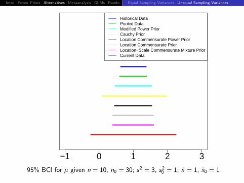
95% BCI for µ given n = 10, n0 = 30; s2 = 3, s20 = 1; x = 1, x0 = 1
Intro Power Priors Alternatives Metaanalysis GLMs Rando DiscussionEqual Sampling Variances Unequal Sampling Variances
−1 0 1 2 3
Historical DataPooled DataModified Power PriorCauchy PriorLocation Commensurate Power PriorLocation Commensurate PriorLocation−Scale Commensurate Mixture PriorCurrent Data
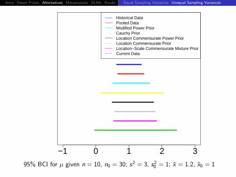
95% BCI for µ given n = 10, n0 = 30; s2 = 3, s20 = 1; x = 1.2, x0 = 1
Intro Power Priors Alternatives Metaanalysis GLMs Rando DiscussionEqual Sampling Variances Unequal Sampling Variances
−1 0 1 2 3
Historical DataPooled DataModified Power PriorCauchy PriorLocation Commensurate Power PriorLocation Commensurate PriorLocation−Scale Commensurate Mixture PriorCurrent Data
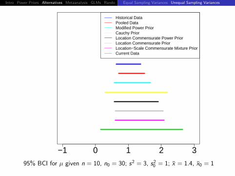
95% BCI for µ given n = 10, n0 = 30; s2 = 3, s20 = 1; x = 1.4, x0 = 1

Intro Power Priors Alternatives Metaanalysis GLMs Rando DiscussionEqual Sampling Variances Unequal Sampling Variances
−1 0 1 2 3
Historical DataPooled DataModified Power PriorCauchy PriorLocation Commensurate Power PriorLocation Commensurate PriorLocation−Scale Commensurate Mixture PriorCurrent Data
95% BCI for µ given n = 10, n0 = 30; s2 = 3, s20 = 1; x = 1.6, x0 = 1
Intro Power Priors Alternatives Metaanalysis GLMs Rando DiscussionEqual Sampling Variances Unequal Sampling Variances
−1 0 1 2 3
Historical DataPooled DataModified Power PriorCauchy PriorLocation Commensurate Power PriorLocation Commensurate PriorLocation−Scale Commensurate Mixture PriorCurrent Data
95% BCI for µ given n = 10, n0 = 30; s2 = 3, s20 = 1; x = 1.8, x0 = 1
Intro Power Priors Alternatives Metaanalysis GLMs Rando DiscussionEqual Sampling Variances Unequal Sampling Variances
−1 0 1 2 3
Historical DataPooled DataModified Power PriorCauchy PriorLocation Commensurate Power PriorLocation Commensurate PriorLocation−Scale Commensurate Mixture PriorCurrent Data
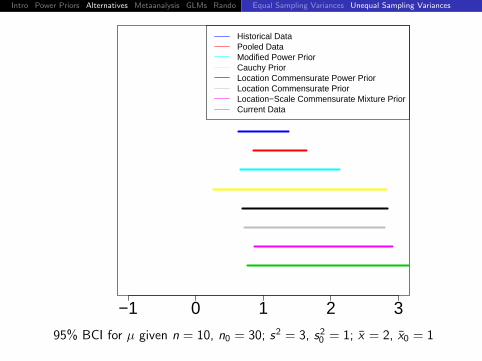
95% BCI for µ given n = 10, n0 = 30; s2 = 3, s20 = 1; x = 2, x0 = 1
Intro Power Priors Alternatives Metaanalysis GLMs Rando Discussion
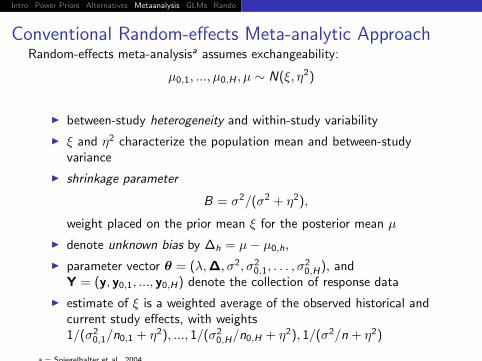
Conventional Random-effects Meta-analytic ApproachRandom-effects meta-analysisa assumes exchangeability:
µ0,1, ..., µ0,H , µ ∼ N(ξ, η2)
I between-study heterogeneity and within-study variability
I ξ and η2 characterize the population mean and between-studyvariance
I shrinkage parameter
B = σ2/(σ2 + η2),
weight placed on the prior mean ξ for the posterior mean µ
I denote unknown bias by ∆h = µ− µ0,h,
I parameter vector θ = (λ,∆, σ2, σ20,1, . . . , σ
20,H), and
Y = (y, y0,1, ..., y0,H) denote the collection of response data
I estimate of ξ is a weighted average of the observed historical andcurrent study effects, with weights1/(σ2
0,1/n0,1 + η2), ..., 1/(σ20,H/n0,H + η2), 1/(σ2/n + η2)
a = Spiegelhalter et al., 2004
Intro Power Priors Alternatives Metaanalysis GLMs Rando Discussion
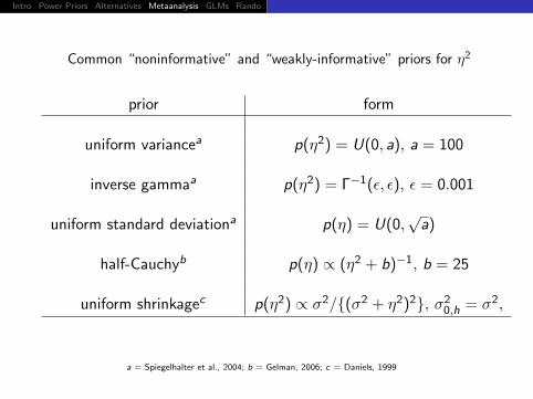
Common “noninformative” and “weakly-informative” priors for η2
prior form
uniform variancea p(η2) = U(0, a), a = 100
inverse gammaa p(η2) = Γ−1(ε, ε), ε = 0.001
uniform standard deviationa p(η) = U(0,√
a)
half-Cauchyb p(η) ∝ (η2 + b)−1, b = 25
uniform shrinkagec p(η2) ∝ σ2/{(σ2 + η2)2}, σ20,h = σ2,
a = Spiegelhalter et al., 2004; b = Gelman, 2006; c = Daniels, 1999
Intro Power Priors Alternatives Metaanalysis GLMs Rando Discussion
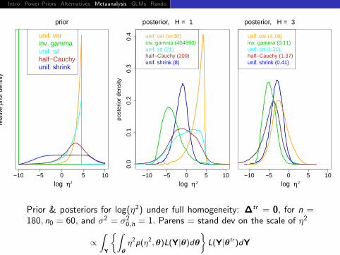
−10 −5 0 5 10
rela
tive
prio
r de
nsity
prior
2ηlog
unif. varinv. gammaunif. sdhalf−Cauchyunif. shrink
−10 −5 0 5 10
0.0
0.1
0.2
0.3
0.4
post
erio
r de
nsity
posterior, H = 1
2ηlog
unif. var (v=30)inv. gamma (404890)unif. sd (21)half−Cauchy (209)unif. shrink (8)
−10 −5 0 5 10
posterior, H = 3
2ηlog
unif. var (4.19)inv. gamma (0.11)unif. sd (1.30)half−Cauchy (1.37)unif. shrink (0.41)
Prior & posteriors for log(η2) under full homogeneity: ∆tr = 0, for n =180, n0 = 60, and σ2 = σ2
0,h = 1. Parens = stand dev on the scale of η2
∝∫
Y
{∫θ
η2p(η2,θ)L(Y|θ)dθ
}L(Y|θtr )dY

Intro Power Priors Alternatives Metaanalysis GLMs Rando Discussion
Commensurate Prior: One Historical Study
I commensurate prior for µ (HCMS, 2011)
µ ∼ N(µ| µ0, 1/τ)
I µ is a “non-systematically biased” representation of µ0
I initial prior, p(µ0), characterizes info. before observing hist. data
I one-to-one relationship between τ and η2: τ = 1/(2η2)
I joint posterior: q(θ|τ, y, y0) ∝
N(µ| µ0, 1/τ)p(µ0)p(σ, σ0)n0∏j=1
N(y0j | µ0, σ20)
n∏i=1
N(yi | µ+ diλ, σ2)
I Pocock (1976) repeated analysis under several fixed values of 1/τ
I HCMS (2011) consider fully Bayesian approaches as well as powerprior formulations

Intro Power Priors Alternatives Metaanalysis GLMs Rando Discussion
Commensurate Prior: One Historical Study (cont’d)
I HSC (2011) proceed with parametric empirical Bayesian inferenceby replacing hyperparameter τ in with its marginal MLE,
τ∗ = arg maxτ∈[lτ ,uτ ]
{m(Y|τ)} ,
restricted to the effective range of borrowing of strength
I Gaussian data, τ∗ ∈ [0.5/102, 0.5/0.052], or η ∈ [0.05, 10]
Our proposed empirical Bayes (EB) procedure:
I “underestimates” variability in θ given that posterior uncertainty inτ∗ is unacknowledged
I offers alternative, (perhaps more desirable) trade-off betweenborrowing of strength and bias
I reduce dimensionality in the numerical marginalization of θ with anormal approx. for non-Gaussian data

Intro Power Priors Alternatives Metaanalysis GLMs Rando Discussion
Commensurate Prior: Multiple Historical Studies
I assume homogeneity among the hist. studies (or fixed degree ofheterogeneity)
I commensurate prior for µ cond. on the hist. population mean:
N(µ| ξ0, 1/τ)
Relationship between τ and η2 is more complicated
I denote v0,h = σ20,h/n0,h, and let v = σ2/(n −
∑di )
I τ−1 characterizes the meta-analytic between-study variability, plusthe diff. between the summed variability among the sample means,and the pop. mean when heterogeneity is estimated η2 versus whenfull homogeneity is assumed,
τ−1 = η2+
{1/(v + η2) +
H∑h=1
1/(v0,h + η2)
}−1−
(1/v +
H∑h=1
1/v0,h
)−1
Intro Power Priors Alternatives Metaanalysis GLMs Rando Discussion
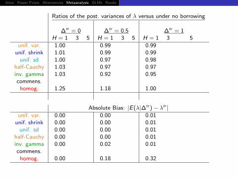
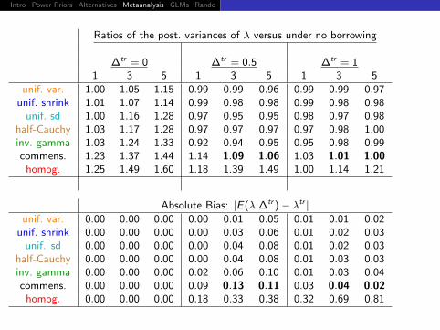
Ratios of the post. variances of λ versus under no borrowing
∆tr = 0 ∆tr = 0.5 ∆tr = 1H = 1 3 5 H = 1 3 5 H = 1 3 5
unif. var. 1.00 0.99 0.99unif. shrink 1.01 0.99 0.99
unif. sd 1.00 0.97 0.98half-Cauchy 1.03 0.97 0.97inv. gamma 1.03 0.92 0.95commens.
homog. 1.25 1.18 1.00
Absolute Bias: |E(λ|∆tr )− λtr |unif. var. 0.00 0.00 0.01
unif. shrink 0.00 0.00 0.01unif. sd 0.00 0.00 0.01
half-Cauchy 0.00 0.00 0.01inv. gamma 0.00 0.02 0.01commens.
homog. 0.00 0.18 0.32
Intro Power Priors Alternatives Metaanalysis GLMs Rando Discussion
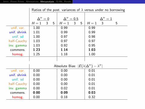
Ratios of the post. variances of λ versus under no borrowing
∆tr = 0 ∆tr = 0.5 ∆tr = 1H = 1 3 5 H = 1 3 5 H = 1 3 5
unif. var. 1.00 0.99 0.99unif. shrink 1.01 0.99 0.99
unif. sd 1.00 0.97 0.98half-Cauchy 1.03 0.97 0.97inv. gamma 1.03 0.92 0.95commens. 1.23 1.14 1.03
homog. 1.25 1.18 1.00
Absolute Bias: |E(λ|∆tr )− λtr |unif. var. 0.00 0.00 0.01
unif. shrink 0.00 0.00 0.01unif. sd 0.00 0.00 0.01
half-Cauchy 0.00 0.00 0.01inv. gamma 0.00 0.02 0.01commens. 0.00 0.09 0.03
homog. 0.00 0.18 0.32
Intro Power Priors Alternatives Metaanalysis GLMs Rando Discussion
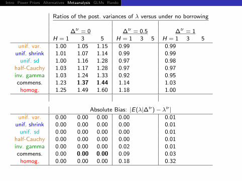
Ratios of the post. variances of λ versus under no borrowing
∆tr = 0 ∆tr = 0.5 ∆tr = 1H = 1 3 5 H = 1 3 5 H = 1 3 5
unif. var. 1.00 1.05 1.15 0.99 0.99unif. shrink 1.01 1.07 1.14 0.99 0.99
unif. sd 1.00 1.16 1.28 0.97 0.98half-Cauchy 1.03 1.17 1.28 0.97 0.97inv. gamma 1.03 1.24 1.33 0.92 0.95commens. 1.23 1.37 1.44 1.14 1.03
homog. 1.25 1.49 1.60 1.18 1.00
Absolute Bias: |E(λ|∆tr )− λtr |unif. var. 0.00 0.00 0.00 0.00 0.01
unif. shrink 0.00 0.00 0.00 0.00 0.01unif. sd 0.00 0.00 0.00 0.00 0.01
half-Cauchy 0.00 0.00 0.00 0.00 0.01inv. gamma 0.00 0.00 0.00 0.02 0.01commens. 0.00 0.00 0.00 0.09 0.03
homog. 0.00 0.00 0.00 0.18 0.32
Intro Power Priors Alternatives Metaanalysis GLMs Rando Discussion
Ratios of the post. variances of λ versus under no borrowing
∆tr = 0 ∆tr = 0.5 ∆tr = 11 3 5 1 3 5 1 3 5
unif. var. 1.00 1.05 1.15 0.99 0.99 0.96 0.99 0.99 0.97unif. shrink 1.01 1.07 1.14 0.99 0.98 0.98 0.99 0.98 0.98
unif. sd 1.00 1.16 1.28 0.97 0.95 0.95 0.98 0.97 0.98half-Cauchy 1.03 1.17 1.28 0.97 0.97 0.97 0.97 0.98 1.00inv. gamma 1.03 1.24 1.33 0.92 0.94 0.95 0.95 0.98 0.99commens. 1.23 1.37 1.44 1.14 1.09 1.06 1.03 1.01 1.00
homog. 1.25 1.49 1.60 1.18 1.39 1.49 1.00 1.14 1.21
Absolute Bias: |E(λ|∆tr )− λtr |unif. var. 0.00 0.00 0.00 0.00 0.01 0.05 0.01 0.01 0.02
unif. shrink 0.00 0.00 0.00 0.00 0.03 0.06 0.01 0.02 0.03unif. sd 0.00 0.00 0.00 0.00 0.04 0.08 0.01 0.02 0.03
half-Cauchy 0.00 0.00 0.00 0.00 0.04 0.08 0.01 0.03 0.03inv. gamma 0.00 0.00 0.00 0.02 0.06 0.10 0.01 0.03 0.04commens. 0.00 0.00 0.00 0.09 0.13 0.11 0.03 0.04 0.02
homog. 0.00 0.00 0.00 0.18 0.33 0.38 0.32 0.69 0.81
Intro Power Priors Alternatives Metaanalysis GLMs Rando DiscussionLogistic Generalized Linear Time-to-Event Mixed Simulations
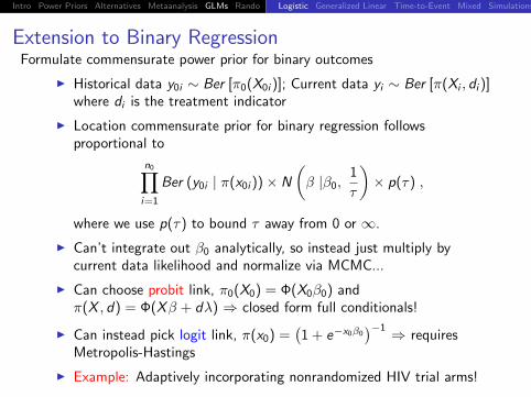
Extension to Binary RegressionFormulate commensurate power prior for binary outcomes
I Historical data y0i ∼ Ber [π0(X0i )]; Current data yi ∼ Ber [π(Xi , di )]where di is the treatment indicator
I Location commensurate prior for binary regression followsproportional to
n0∏i=1
Ber (y0i | π(x0i ))× N
(β |β0,
1
τ
)× p(τ) ,
where we use p(τ) to bound τ away from 0 or ∞.
I Can’t integrate out β0 analytically, so instead just multiply bycurrent data likelihood and normalize via MCMC...
I Can choose probit link, π0(X0) = Φ(X0β0) andπ(X , d) = Φ(Xβ + dλ) ⇒ closed form full conditionals!
I Can instead pick logit link, π(x0) =(1 + e−x0β0
)−1 ⇒ requiresMetropolis-Hastings
I Example: Adaptively incorporating nonrandomized HIV trial arms!

Intro Power Priors Alternatives Metaanalysis GLMs Rando DiscussionLogistic Generalized Linear Time-to-Event Mixed Simulations
Extension to Generalized Linear Models
I Assume an initial flat prior on β0, and use the “Bayesian CentralLimit Theorem” with the historical likelihood to obtain
β0·∼ N
(β0, Σ0
),
where β0 is the historical MLE for β0, and Σ0 is the inverse of thehistorical observed Fisher information matrix
I Specifying a flat prior for λ, a N(β0,1τ Ip) prior for β, and integrating
out β0 again leads to joint location commensurate prior of
p(β, λ, τ |y0) ∝ Np
(V−1M,
1
τV−1
)p(τ)
I The joint posterior follows by multiplying by the current datalikelihood, which yields intractable full conditionals. Here we useMetropolis-Hastings (NOT the BCLT again, which would requirefixed β and λ in the Fisher information matrix)
I Primary target application: formulation for survival outcomes...
Intro Power Priors Alternatives Metaanalysis GLMs Rando DiscussionLogistic Generalized Linear Time-to-Event Mixed Simulations
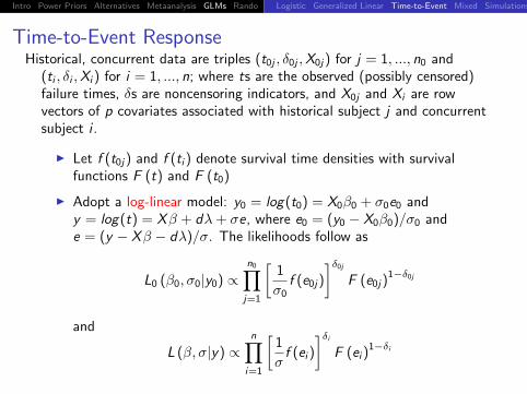
Time-to-Event ResponseHistorical, concurrent data are triples (t0j , δ0j ,X0j) for j = 1, ..., n0 and
(ti , δi ,Xi ) for i = 1, ..., n; where ts are the observed (possibly censored)failure times, δs are noncensoring indicators, and X0j and Xi are rowvectors of p covariates associated with historical subject j and concurrentsubject i .
I Let f (t0j) and f (ti ) denote survival time densities with survivalfunctions F (t) and F (t0)
I Adopt a log-linear model: y0 = log(t0) = X0β0 + σ0e0 andy = log(t) = Xβ + dλ+ σe, where e0 = (y0 − X0β0)/σ0 ande = (y − Xβ − dλ)/σ. The likelihoods follow as
L0 (β0, σ0|y0) ∝n0∏j=1
[1
σ0f (e0j)
]δ0jF (e0j)
1−δ0j
and
L (β, σ|y) ∝n∏
i=1
[1
σf (ei )
]δiF (ei )
1−δi
Intro Power Priors Alternatives Metaanalysis GLMs Rando DiscussionLogistic Generalized Linear Time-to-Event Mixed Simulations
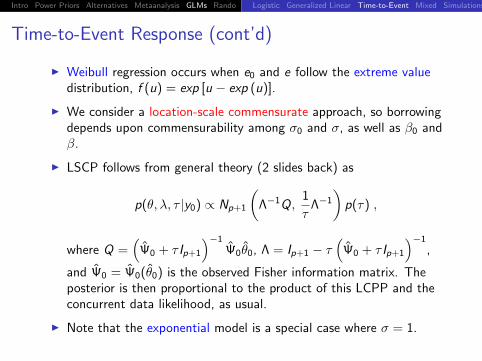
Time-to-Event Response (cont’d)
I Weibull regression occurs when e0 and e follow the extreme valuedistribution, f (u) = exp [u − exp (u)].
I We consider a location-scale commensurate approach, so borrowingdepends upon commensurability among σ0 and σ, as well as β0 andβ.
I LSCP follows from general theory (2 slides back) as
p(θ, λ, τ |y0) ∝ Np+1
(Λ−1Q,
1
τΛ−1
)p(τ) ,
where Q =(
Ψ0 + τ Ip+1
)−1Ψ0θ0, Λ = Ip+1 − τ
(Ψ0 + τ Ip+1
)−1,
and Ψ0 = Ψ0(θ0) is the observed Fisher information matrix. Theposterior is then proportional to the product of this LCPP and theconcurrent data likelihood, as usual.
I Note that the exponential model is a special case where σ = 1.

Intro Power Priors Alternatives Metaanalysis GLMs Rando DiscussionLogistic Generalized Linear Time-to-Event Mixed Simulations
Extension to General/Generalized Mixed ModelsConsider the Gaussian case for now (non-Gaussian also feasible):
I historical data: y0ij , i = 1, . . . , n0j , j = 1, . . . ,m0; arrange in avector y0 and model as y0 = X0β0 + Z0u0 + ε0, where
E
(u0
ε0
)=
(0
0
)and Cov
(u0
ε0
)=
(G0 00 R0
)I current data: uses similar notation: y = Xβ + dλ+ Zu + ε, where
d is a N × 1 indicator of treatment.
I The location commensurate prior emerges as proportional to
Np
(β V−1M,
1
τV−1
)× Nm
(u 0, σ2
uIm)× p(λ, σε, σu, τ),
where M =(
XT0 Σ−1X0 + τ Ip
)−1XT0 Σ−1X0β0,
V = Ip − τ(
XT0 Σ−1X0 + τ Ip
)−1, and β0 is the BLUE.
I As usual, multiply by current data likelihood and normalize; fullconditionals are normal and inverse Wishart; non-Gaussian caserequires Metropolis-Hastings
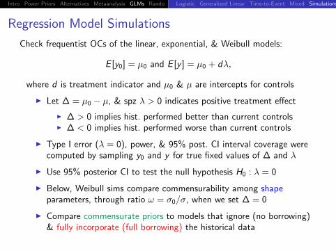
Intro Power Priors Alternatives Metaanalysis GLMs Rando DiscussionLogistic Generalized Linear Time-to-Event Mixed Simulations
Regression Model Simulations
Check frequentist OCs of the linear, exponential, & Weibull models:
E [y0] = µ0 and E [y ] = µ0 + dλ,
where d is treatment indicator and µ0 & µ are intercepts for controls
I Let ∆ = µ0 − µ, & spz λ > 0 indicates positive treatment effect
I ∆ > 0 implies hist. performed better than current controlsI ∆ < 0 implies hist. performed worse than current controls
I Type I error (λ = 0), power, & 95% post. CI interval coverage werecomputed by sampling y0 and y for true fixed values of ∆ and λ
I Use 95% posterior CI to test the null hypothesis H0 : λ = 0
I Below, Weibull sims compare commensurability among shapeparameters, through ratio ω = σ0/σ, when we set ∆ = 0
I Compare commensurate priors to models that ignore (no borrowing)& fully incorporate (full borrowing) the historical data
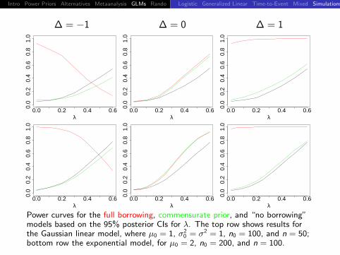
Intro Power Priors Alternatives Metaanalysis GLMs Rando DiscussionLogistic Generalized Linear Time-to-Event Mixed Simulations
∆ = −1 ∆ = 0 ∆ = 1
0.0 0.2 0.4 0.6
0.0
0.2
0.4
0.6
0.8
1.0
λ0.0 0.2 0.4 0.6
0.0
0.2
0.4
0.6
0.8
1.0
λ0.0 0.2 0.4 0.6
0.0
0.2
0.4
0.6
0.8
1.0
λ
0.0 0.2 0.4 0.6
0.0
0.2
0.4
0.6
0.8
1.0
λ0.0 0.2 0.4 0.6
0.0
0.2
0.4
0.6
0.8
1.0
λ0.0 0.2 0.4 0.6
0.0
0.2
0.4
0.6
0.8
1.0
λ
Power curves for the full borrowing, commensurate prior, and “no borrowing”models based on the 95% posterior CIs for λ. The top row shows results forthe Gaussian linear model, where µ0 = 1, σ2
0 = σ2 = 1, n0 = 100, and n = 50;bottom row the exponential model, for µ0 = 2, n0 = 200, and n = 100.
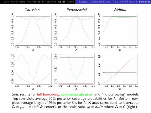
Intro Power Priors Alternatives Metaanalysis GLMs Rando DiscussionLogistic Generalized Linear Time-to-Event Mixed Simulations
Gaussian Exponential Weibull
−1.5 −0.5 0.5 1.5
0.0
0.2
0.4
0.6
0.8
1.0
∆−1.0 −0.5 0.0 0.5 1.0
0.0
0.2
0.4
0.6
0.8
1.0
∆0.5 1.0 1.5 2.0 2.5 3.0
0.0
0.2
0.4
0.6
0.8
1.0
ω
−1.5 −0.5 0.5 1.5
0.90
1.00
1.10
1.20
∆−1.0 −0.5 0.0 0.5 1.0
0.70
0.80
0.90
∆0.5 1.0 1.5 2.0 2.5 3.0
0.4
0.8
1.2
1.6
ω
Sim. results for full borrowing, commensurate prior, and “no borrowing” models.Top row plots average 95% posterior coverage probabilities for λ. Bottom rowplots average length of 95% posterior CIs for λ. X-axes correspond to intercepts,∆ = µ0 − µ (left & center), or the scale ratio, ω = σ0/σ where ∆ = 0 (right).

Intro Power Priors Alternatives Metaanalysis GLMs Rando Discussion
Adaptive Randomization
Friedman, Furberg, and DeMets (1998, p.69) broadly refer torandomization procedures that adjust the allocation ratio as the studyprogresses as adaptive. Commonly used to
I balance prognostic factors among the intervention arms
I assign patients to the better performing regimen in early phase trials
Commensurate prior models for controlled trials naturally advocate arandomization scheme that is “optimal” with respect to the amountstrength borrowed from the historical controls
I Use more of the new patients to learn about the efficacy and safetyprofile of the new intervention
I Adjust prob. of allocating next patient to new intervention accordingto the commensurability of the historical and current controls
I Evaluate sequentially using repeated fitting
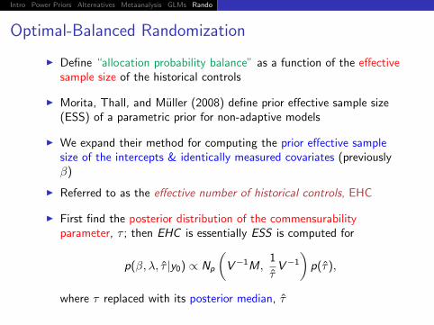
Intro Power Priors Alternatives Metaanalysis GLMs Rando Discussion
Optimal-Balanced Randomization
I Define “allocation probability balance” as a function of the effectivesample size of the historical controls
I Morita, Thall, and Muller (2008) define prior effective sample size(ESS) of a parametric prior for non-adaptive models
I We expand their method for computing the prior effective samplesize of the intercepts & identically measured covariates (previouslyβ)
I Referred to as the effective number of historical controls, EHC
I First find the posterior distribution of the commensurabilityparameter, τ ; then EHC is essentially ESS is computed for
p(β, λ, τ |y0) ∝ Np
(V−1M,
1
τV−1
)p(τ),
where τ replaced with its posterior median, τ
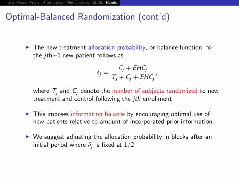
Intro Power Priors Alternatives Metaanalysis GLMs Rando Discussion
Optimal-Balanced Randomization (cont’d)
I The new treatment allocation probability, or balance function, forthe jth+1 new patient follows as
δj =Cj + EHCj
Tj + Cj + EHCj,
where Tj and Cj denote the number of subjects randomized to newtreatment and control following the jth enrollment
I This imposes information balance by encouraging optimal use ofnew patients relative to amount of incorporated prior information
I We suggest adjusting the allocation probability in blocks after aninitial period where δj is fixed at 1/2
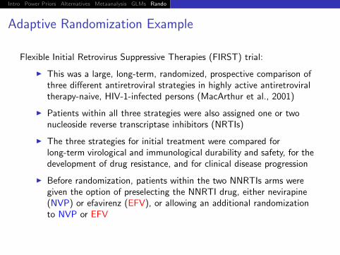
Intro Power Priors Alternatives Metaanalysis GLMs Rando Discussion
Adaptive Randomization Example
Flexible Initial Retrovirus Suppressive Therapies (FIRST) trial:
I This was a large, long-term, randomized, prospective comparison ofthree different antiretroviral strategies in highly active antiretroviraltherapy-naive, HIV-1-infected persons (MacArthur et al., 2001)
I Patients within all three strategies were also assigned one or twonucleoside reverse transcriptase inhibitors (NRTIs)
I The three strategies for initial treatment were compared forlong-term virological and immunological durability and safety, for thedevelopment of drug resistance, and for clinical disease progression
I Before randomization, patients within the two NNRTIs arms weregiven the option of preselecting the NNRTI drug, either nevirapine(NVP) or efavirenz (EFV), or allowing an additional randomizationto NVP or EFV
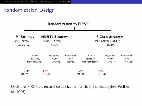
Intro Power Priors Alternatives Metaanalysis GLMs Rando Discussion
Randomization Design
Randomization to FIRST
PI Strategy(PI + NRTIs)
(data not used)
NNRTI Strategy(NNRTI + NRTIs)
N=409
NNRTI
substudy
Randomization
Prescribed
NVP
(N=100)
Prescribed
EFV
(N=211)
NVP
(N=50)
EFV
(N=48)
3-Class Strategy(PI + NNRTI + NRTIs)
N=403
NNRTI
substudy
Randomization
Prescribed
NVP
(N=137)
Prescribed
EFV
(N=161)
NVP
(N=51)
EFV
(N=54)
Outline of FIRST design and randomization for eligible subjects (Berg-Wolf et
al., 2006).
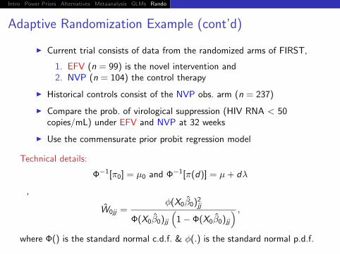
Intro Power Priors Alternatives Metaanalysis GLMs Rando Discussion
Adaptive Randomization Example (cont’d)
I Current trial consists of data from the randomized arms of FIRST,
1. EFV (n = 99) is the novel intervention and2. NVP (n = 104) the control therapy
I Historical controls consist of the NVP obs. arm (n = 237)
I Compare the prob. of virological suppression (HIV RNA < 50copies/mL) under EFV and NVP at 32 weeks
I Use the commensurate prior probit regression model
Technical details:
Φ−1[π0] = µ0 and Φ−1[π(d)] = µ+ dλ
,
W0jj =φ(X0β0)2jj
Φ(X0β0)jj(
1− Φ(X0β0)jj) ,
where Φ() is the standard normal c.d.f. & φ(.) is the standard normal p.d.f.
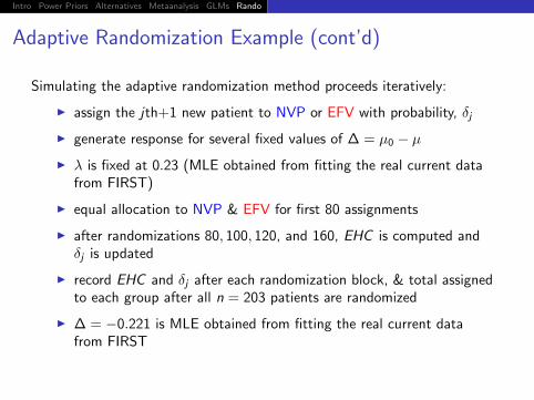
Intro Power Priors Alternatives Metaanalysis GLMs Rando Discussion
Adaptive Randomization Example (cont’d)
Simulating the adaptive randomization method proceeds iteratively:
I assign the jth+1 new patient to NVP or EFV with probability, δj
I generate response for several fixed values of ∆ = µ0 − µI λ is fixed at 0.23 (MLE obtained from fitting the real current data
from FIRST)
I equal allocation to NVP & EFV for first 80 assignments
I after randomizations 80, 100, 120, and 160, EHC is computed andδj is updated
I record EHC and δj after each randomization block, & total assignedto each group after all n = 203 patients are randomized
I ∆ = −0.221 is MLE obtained from fitting the real current datafrom FIRST
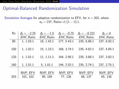
Intro Power Priors Alternatives Metaanalysis GLMs Rando Discussion
Optimal-Balanced Randomization Simulation
Simulation Averages for adaptive randomization to EFV, for n = 203, wheren0 = 237, Ratio=δ/(1− δ):1.
Rz ∆ = −2.25 ∆ = −1.5 ∆ = −0.75 ∆ = −0.221 ∆ = 0EHC ,Ratio EHC ,Ratio EHC ,Ratio EHC ,Ratio EHC ,Ratio
80 1, 1.03:1 18, 1.42:1 177, 5.43:1 235, 6.86:1 237, 6.92:1
100 1, 1.02:1 15, 1.23:1 168, 3.74:1 235, 4.82:1 237, 4.85:1
120 1, 1.01:1 11, 1.11:1 164, 2.95:1 235, 3.80:1 237, 3.82:1
160 1, 1.01:1 5, 1.01:1 144, 2.02:1 235, 2.74:1 237, 2.75:1
NVP, EFV NVP, EFV NVP, EFV NVP, EFV NVP, EFV203 101, 102 99, 104 77, 126 66, 137 65, 138

Intro Power Priors Alternatives Metaanalysis GLMs Rando DiscussionConclusion
Is all of this “legal”?
I X-L Meng: NO: Agreement between the historical andconcurrent data does not necessarily imply they are studyingthe same thing! External validation/information is alwaysrequired!
I (Fairly hardcore) frequentist referee: Not yet: One needs to“evaluate theoretical properties, such as Bernstein-von Misestype results [showing asymptotic equivalence between Bayesand frequentist results] to provide some kind of universalassurances and/or insight beyond simulations into when gainscan be expected.”
I BP Carlin: Yes: Point taken, but our goal here was never to“match” frequentist results, and moreover the frequentistsimulations we have carried out speak for themsselves and are“Bayesianly justified” in the sense of Rubin (1984)!

Intro Power Priors Alternatives Metaanalysis GLMs Rando DiscussionConclusion
ConclusionI Adaptive borrowing is consistent with recent arguments on
behalf of the ease and desirability of adaptivity in Bayesianclinical trials generally; c.f. new Chapman and Hall textbookby Berry, Carlin, Lee, and Muller (2010)!
Papers related to this work:
I Hobbs, B.P., Carlin, B.P., Mandrekar, S., and Sargent, D.J.(2011). Hierarchical commensurate and power prior modelsfor adaptive incorporation of historical information in clinicaltrials. Biometrics, 67, 1047–1056.
I Hobbs, B.P., Sargent, D.J., and Carlin, B.P. (2010).Commensurate priors for incorporating historical informationin clinical trials using general and generalized linear models.Under revision for Bayesian Analysis.
I Hobbs, B.P. and Carlin, B.P. (2012). Optimal-balancedrandomization for controlled clinical trials that incorporatehistorical controls. Manuscript in process.

Bayesian Hierarchical Modeling
for Detecting Safety Signals
in Clinical Trials
Amy Xia, Amgen, Inc.
Haijun Ma, Amgen, Inc.
Brad Carlin, University of Minnesota
Medtronic Statistics Conference
Minneapolis, MN, October 4, 2011

Outline
• Introduction
• Why Are Bayesian Models Helpful?
• Three Stage Bayesian Hierarchical Models
• An Example
• Simulation Study
• Closing Remarks
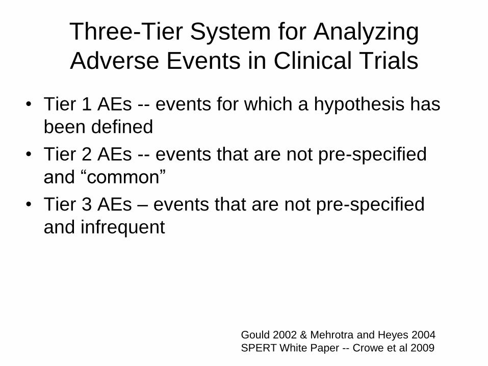
Three-Tier System for Analyzing
Adverse Events in Clinical Trials
• Tier 1 AEs -- events for which a hypothesis has
been defined
• Tier 2 AEs -- events that are not pre-specified
and “common”
• Tier 3 AEs – events that are not pre-specified
and infrequent
Gould 2002 & Mehrotra and Heyes 2004
SPERT White Paper -- Crowe et al 2009
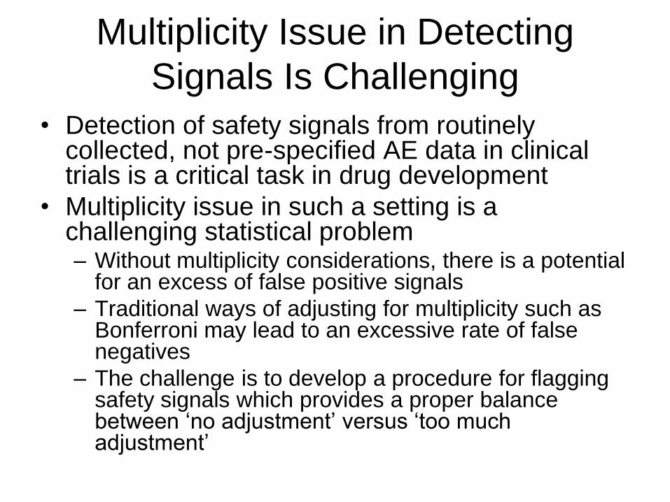
Multiplicity Issue in Detecting
Signals Is Challenging
• Detection of safety signals from routinely collected, not pre-specified AE data in clinical trials is a critical task in drug development
• Multiplicity issue in such a setting is a challenging statistical problem – Without multiplicity considerations, there is a potential
for an excess of false positive signals
– Traditional ways of adjusting for multiplicity such as Bonferroni may lead to an excessive rate of false negatives
– The challenge is to develop a procedure for flagging safety signals which provides a proper balance between „no adjustment‟ versus „too much adjustment‟
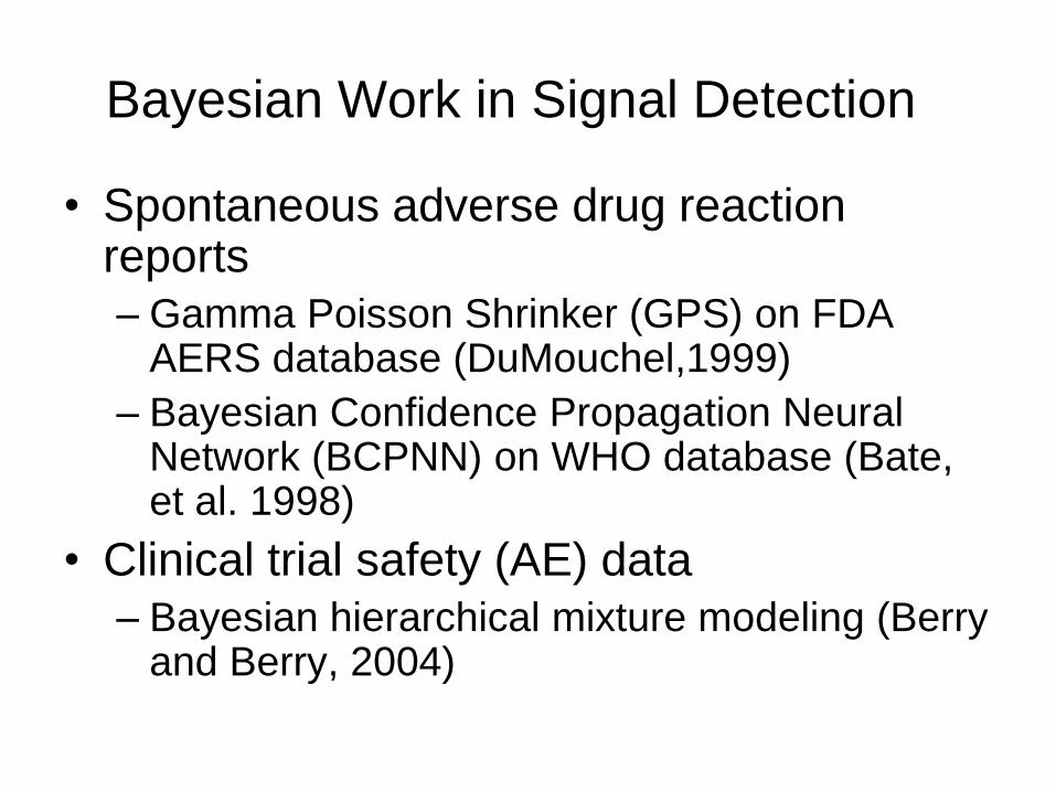
Bayesian Work in Signal Detection
• Spontaneous adverse drug reaction reports
– Gamma Poisson Shrinker (GPS) on FDA AERS database (DuMouchel,1999)
– Bayesian Confidence Propagation Neural Network (BCPNN) on WHO database (Bate, et al. 1998)
• Clinical trial safety (AE) data
– Bayesian hierarchical mixture modeling (Berry and Berry, 2004)

“Safety assessment is one area
where frequentist strategies have
been less applicable. Perhaps
Bayesian approaches in this area
have more promise.”
-- Chi, Hung, and O‟Neill;
Pharmaceutical Report, 2002
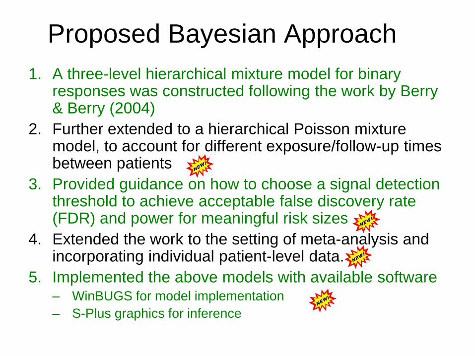
Proposed Bayesian Approach
1. A three-level hierarchical mixture model for binary responses was constructed following the work by Berry & Berry (2004)
2. Further extended to a hierarchical Poisson mixture model, to account for different exposure/follow-up times between patients
3. Provided guidance on how to choose a signal detection threshold to achieve acceptable false discovery rate (FDR) and power for meaningful risk sizes
4. Extended the work to the setting of meta-analysis and incorporating individual patient-level data.
5. Implemented the above models with available software – WinBUGS for model implementation
– S-Plus graphics for inference
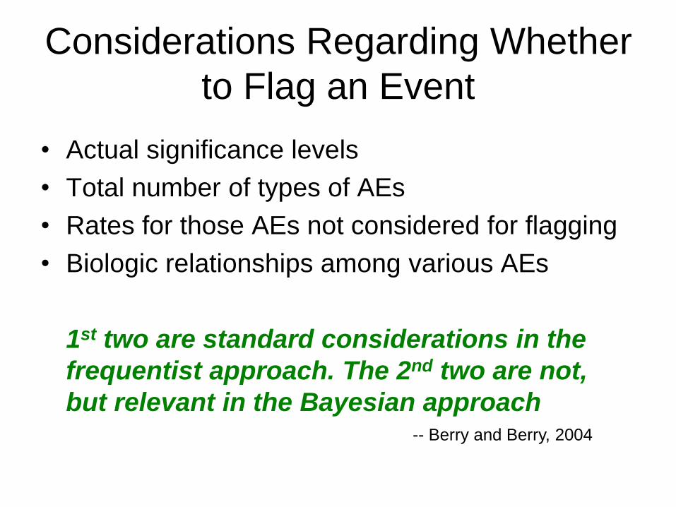
Considerations Regarding Whether
to Flag an Event
• Actual significance levels
• Total number of types of AEs
• Rates for those AEs not considered for flagging
• Biologic relationships among various AEs
1st two are standard considerations in the
frequentist approach. The 2nd two are not,
but relevant in the Bayesian approach
-- Berry and Berry, 2004
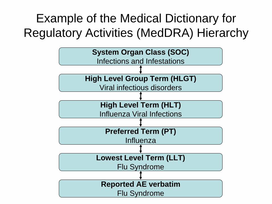
Example of the Medical Dictionary for
Regulatory Activities (MedDRA) Hierarchy
System Organ Class (SOC)
Infections and Infestations
High Level Group Term (HLGT)
Viral infectious disorders
High Level Term (HLT)
Influenza Viral Infections
Preferred Term (PT)
Influenza
Lowest Level Term (LLT)
Flu Syndrome
Reported AE verbatim
Flu Syndrome
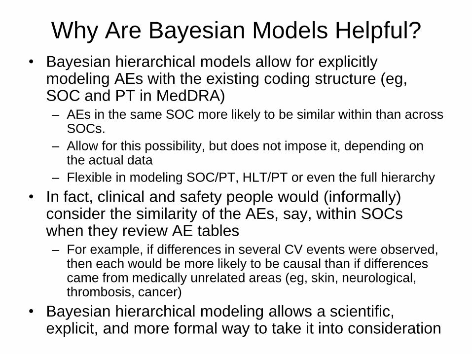
Why Are Bayesian Models Helpful?
• Bayesian hierarchical models allow for explicitly modeling AEs with the existing coding structure (eg, SOC and PT in MedDRA) – AEs in the same SOC more likely to be similar within than across
SOCs.
– Allow for this possibility, but does not impose it, depending on the actual data
– Flexible in modeling SOC/PT, HLT/PT or even the full hierarchy
• In fact, clinical and safety people would (informally) consider the similarity of the AEs, say, within SOCs when they review AE tables – For example, if differences in several CV events were observed,
then each would be more likely to be causal than if differences came from medically unrelated areas (eg, skin, neurological, thrombosis, cancer)
• Bayesian hierarchical modeling allows a scientific, explicit, and more formal way to take it into consideration
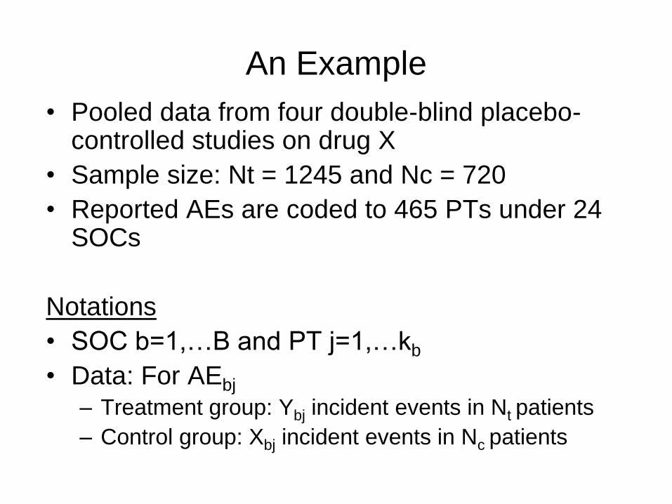
An Example
• Pooled data from four double-blind placebo-controlled studies on drug X
• Sample size: Nt = 1245 and Nc = 720
• Reported AEs are coded to 465 PTs under 24 SOCs
Notations
• SOC b=1,…B and PT j=1,…kb
• Data: For AEbj – Treatment group: Ybj incident events in Nt patients
– Control group: Xbj incident events in Nc patients
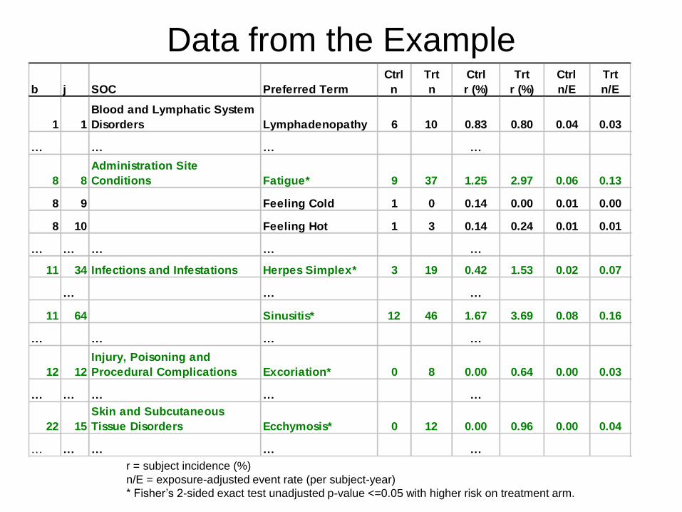
r = subject incidence (%)
n/E = exposure-adjusted event rate (per subject-year)
* Fisher‟s 2-sided exact test unadjusted p-value <=0.05 with higher risk on treatment arm.
Data from the Example
b j SOC Preferred Term
Ctrl
n
Trt
n
Ctrl
r (%)
Trt
r (%)
Ctrl
n/E
Trt
n/E
1 1
Blood and Lymphatic System
Disorders Lymphadenopathy 6 10 0.83 0.80 0.04 0.03
… … … …
8 8
General Disorders and
Administration Site
Conditions Fatigue* 9 37 1.25 2.97 0.06 0.13
8 9 Feeling Cold 1 0 0.14 0.00 0.01 0.00
8 10 Feeling Hot 1 3 0.14 0.24 0.01 0.01
… … … … …
11 34 Infections and Infestations Herpes Simplex* 3 19 0.42 1.53 0.02 0.07
… … …
11 64 Sinusitis* 12 46 1.67 3.69 0.08 0.16
… … … …
12 12
Injury, Poisoning and
Procedural Complications Excoriation* 0 8 0.00 0.64 0.00 0.03
… … … … …
22 15
Skin and Subcutaneous
Tissue Disorders Ecchymosis* 0 12 0.00 0.96 0.00 0.04
… … … … …
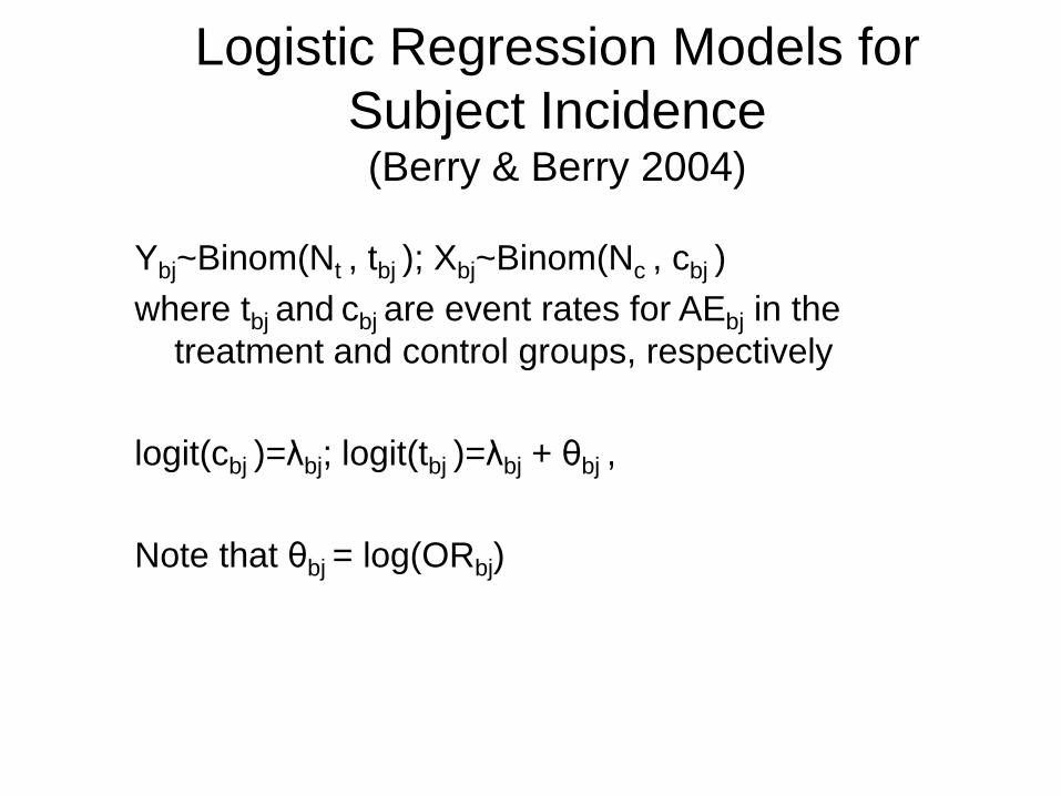
Logistic Regression Models for
Subject Incidence (Berry & Berry 2004)
Ybj~Binom(Nt , tbj ); Xbj~Binom(Nc , cbj )
where tbj and cbj are event rates for AEbj in the
treatment and control groups, respectively
logit(cbj )=λbj; logit(tbj )=λbj + θbj ,
Note that θbj = log(ORbj)
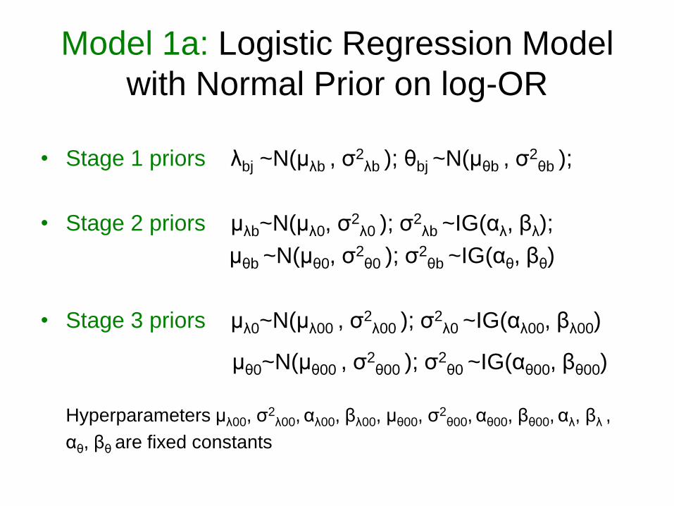
Model 1a: Logistic Regression Model
with Normal Prior on log-OR
• Stage 1 priors λbj ~N(μλb , σ2
λb ); θbj ~N(μθb , σ2
θb );
• Stage 2 priors μλb~N(μλ0, σ2
λ0 ); σ2
λb ~IG(αλ, βλ);
μθb ~N(μθ0, σ2
θ0 ); σ2
θb ~IG(αθ, βθ)
• Stage 3 priors μλ0~N(μλ00 , σ2
λ00 ); σ2
λ0 ~IG(αλ00, βλ00)
μθ0~N(μθ00 , σ2
θ00 ); σ2
θ0 ~IG(αθ00, βθ00)
Hyperparameters μλ00, σ2
λ00, αλ00, βλ00, μθ00, σ2
θ00, αθ00, βθ00, αλ, βλ ,
αθ, βθ are fixed constants
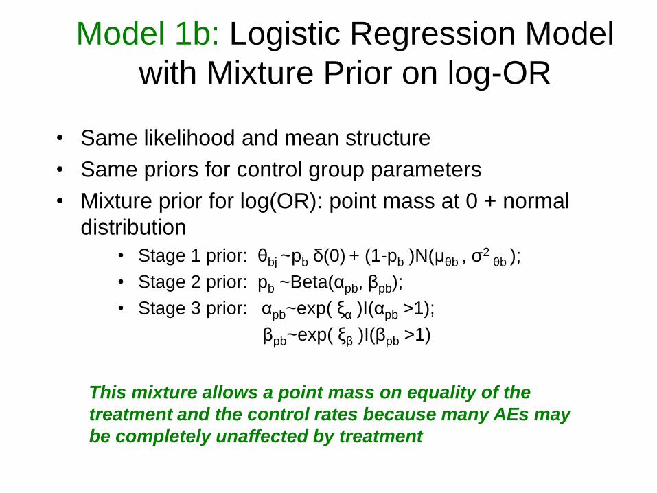
Model 1b: Logistic Regression Model
with Mixture Prior on log-OR
• Same likelihood and mean structure
• Same priors for control group parameters
• Mixture prior for log(OR): point mass at 0 + normal
distribution
• Stage 1 prior: θbj ~pb δ(0) + (1-pb )N(μθb , σ2
θb );
• Stage 2 prior: pb ~Beta(αpb, βpb);
• Stage 3 prior: αpb~exp( ξα )I(αpb >1);
βpb~exp( ξβ )I(βpb >1)
This mixture allows a point mass on equality of the
treatment and the control rates because many AEs may
be completely unaffected by treatment
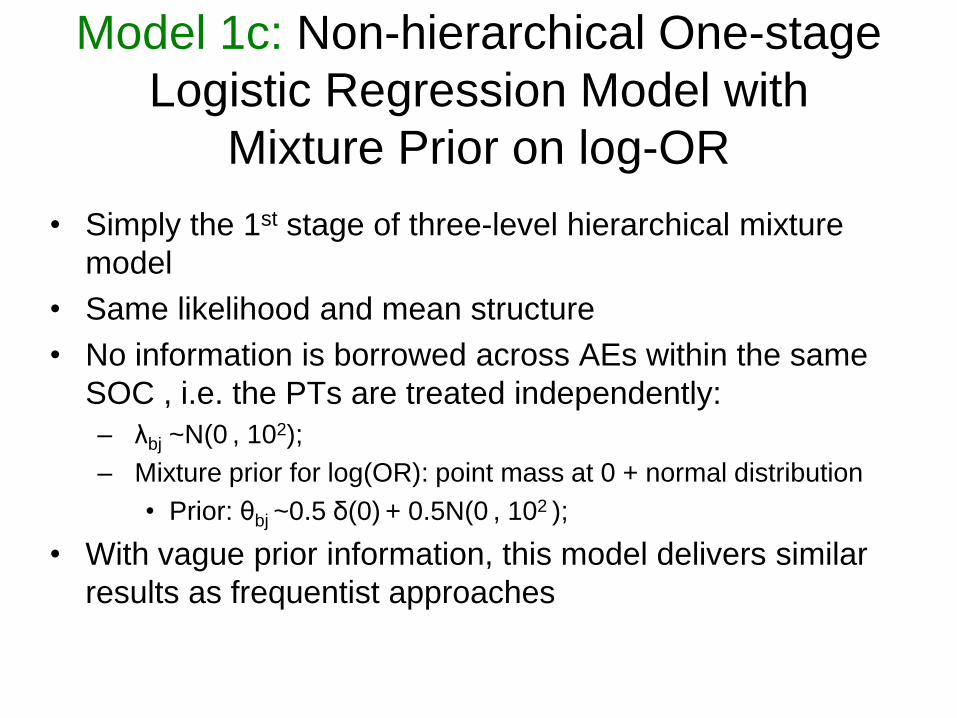
Model 1c: Non-hierarchical One-stage
Logistic Regression Model with
Mixture Prior on log-OR
• Simply the 1st stage of three-level hierarchical mixture
model
• Same likelihood and mean structure
• No information is borrowed across AEs within the same
SOC , i.e. the PTs are treated independently:
– λbj ~N(0 , 102);
– Mixture prior for log(OR): point mass at 0 + normal distribution
• Prior: θbj ~0.5 δ(0) + 0.5N(0 , 102 );
• With vague prior information, this model delivers similar
results as frequentist approaches
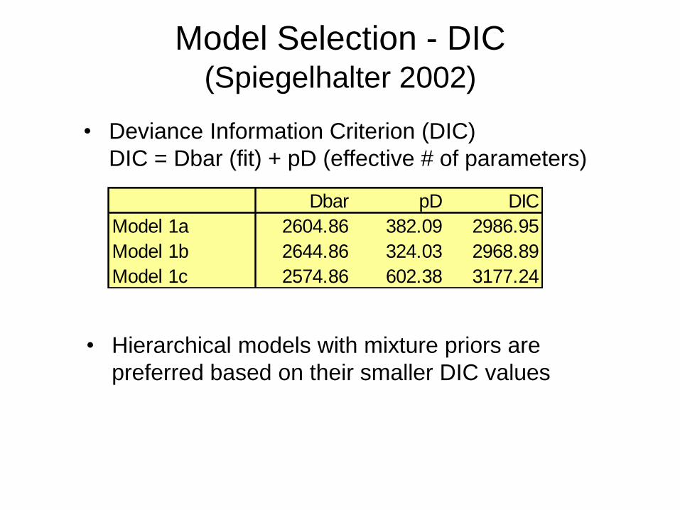
Model Selection - DIC (Spiegelhalter 2002)
• Hierarchical models with mixture priors are
preferred based on their smaller DIC values
Dbar pD DIC
Model 1a 2604.86 382.09 2986.95
Model 1b 2644.86 324.03 2968.89
Model 1c 2574.86 602.38 3177.24
• Deviance Information Criterion (DIC)
DIC = Dbar (fit) + pD (effective # of parameters)
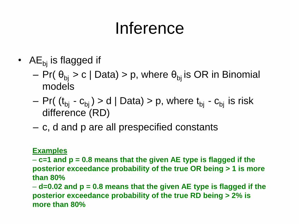
Inference
• AEbj is flagged if
– Pr( θbj > c | Data) > p, where θbj is OR in Binomial
models
– Pr( (tbj - cbj ) > d | Data) > p, where tbj - cbj is risk
difference (RD)
– c, d and p are all prespecified constants
Examples
– c=1 and p = 0.8 means that the given AE type is flagged if the
posterior exceedance probability of the true OR being > 1 is more
than 80%
– d=0.02 and p = 0.8 means that the given AE type is flagged if the
posterior exceedance probability of the true RD being > 2% is
more than 80%
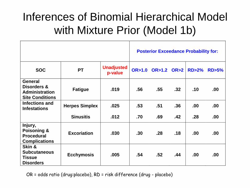
Inferences of Binomial Hierarchical Model
with Mixture Prior (Model 1b)
Posterior Exceedance Probability for:
SOC PT Unadjusted
p-value OR>1.0 OR>1.2 OR>2 RD>2% RD>5%
General Disorders & Administration Site Conditions
Fatigue .019 .56 .55 .32 .10 .00
Infections and Infestations
Herpes Simplex .025 .53 .51 .36 .00 .00
Sinusitis .012 .70 .69 .42 .28 .00
Injury, Poisoning & Procedural Complications
Excoriation .030 .30 .28 .18 .00 .00
Skin & Subcutaneous Tissue Disorders
Ecchymosis .005 .54 .52 .44 .00 .00
OR = odds ratio (drug:placebo), RD = risk difference (drug - placebo)
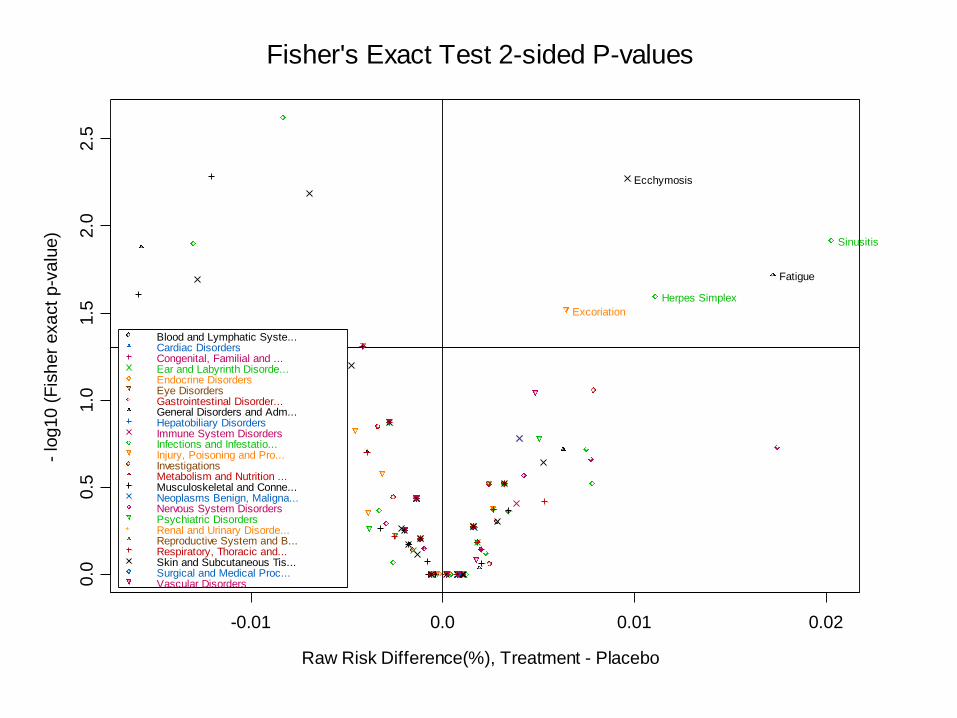
Fisher's Exact Test 2-sided P-values
Raw Risk Difference(%), Treatment - Placebo
- lo
g10
(F
ish
er
exa
ct
p-v
alu
e)
-0.01 0.0 0.01 0.02
0.0
0.5
1.0
1.5
2.0
2.5
Fatigue
Herpes Simplex
Sinusitis
Excoriation
Ecchymosis
Blood and Lymphatic Syste...Cardiac DisordersCongenital, Familial and ...Ear and Labyrinth Disorde...Endocrine DisordersEye DisordersGastrointestinal Disorder...General Disorders and Adm...Hepatobiliary DisordersImmune System DisordersInfections and Infestatio...Injury, Poisoning and Pro...InvestigationsMetabolism and Nutrition ...Musculoskeletal and Conne...Neoplasms Benign, Maligna...Nervous System DisordersPsychiatric DisordersRenal and Urinary Disorde...Reproductive System and B...Respiratory, Thoracic and...Skin and Subcutaneous Tis...Surgical and Medical Proc...Vascular Disorders
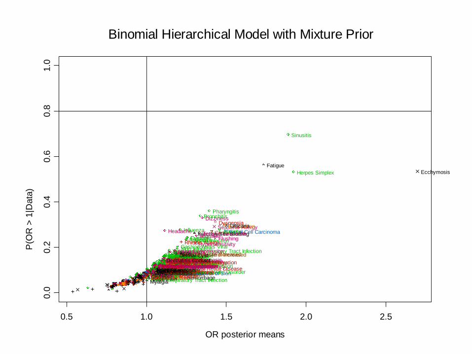
Binomial Hierarchical Model with Mixture Prior
OR posterior means
P(O
R >
1|D
ata
)
0.5 1.0 1.5 2.0 2.5
0.0
0.2
0.4
0.6
0.8
1.0
Lymphadenopathy Ear Pain Tinnitus
Vertigo
Vertigo Positional Cataract
Conjunctival Haemorrhage
Conjunctivitis
Conjunctivitis Allergic Diplopia
Dry Eye
Eye Haemorrhage Eye Inflammation Eye Irritation Eye Pruritus Eyelid Oedema Vision Blurred Abdominal Distension
Abdominal Pain Abdominal Pain Upper
Diarrhoea Dry Mouth
Dyspepsia
Flatulence Food Poisoning
Gastrointestinal Inflammation Gastrooesophageal Reflux Disease
Nausea Stomach Discomfort Toothache
Fatigue
Feeling Hot
Injection Site Bruising
Injection Site Haemorrhage
Malaise
Hypersensitivity
Seasonal Allergy
Abdominal Infection Acute Sinusitis Appendicitis
Bronchitis
Bronchitis Chronic
Candidiasis Cat Scratch Disease Cellulitis Staphylococcal Cervicitis Condyloma Acuminatum
Cystitis
Diverticulitis
Ear Infection
Erysipelas Eyelid Infection
Folliculitis
Fungal Infection
Furuncle
Gastroenteritis Viral
Genital Infection Female Gingival Infection
Herpes Simplex
Herpes Virus Infection Herpes Zoster
Impetigo
Infected Insect Bite
Infected Sebaceous Cyst Infectious Mononucleosis
Influenza
Labyrinthitis Laryngitis
Lower Respiratory Tract Infection Mastitis
Nasopharyngitis
Onychomycosis
Oral Candidiasis Oral Pustule
Otitis Externa Otitis Media
Pharyngitis
Pneumonia Postoperative Infection Pulpitis Dental Puncture Site Infection Rash Pustular
Rhinitis
Sialoadenitis
Sinusitis
Skin Infection
Subcutaneous Abscess Tinea Cruris Tinea Infection Tinea Pedis
Tinea Versicolour Tonsillitis
Tooth Abscess Tooth Infection
Upper Respiratory Tract Infection
Vaginal Candidiasis
Vaginal Infection
Vaginal Mycosis
Viral Infection
Viral Pharyngitis
Viral Upper Respiratory Tract Infection
Animal Bite Contusion
Excoriation
Fall Foot Fracture Hand Fracture Muscle Strain
Pain Trauma Activated
Road Traffic Accident Skin Laceration Sunburn Thermal Burn Tooth Injury Wound
Blood Cholesterol Increased
Blood Glucose Increased
Blood Pressure Increased
Body Temperature Increased Weight Decreased Weight Increased Decreased Appetite Back Pain
Myalgia
Shoulder Pain Tendonitis
Basal Cell Carcinoma
Fibrous Histiocytoma
Seborrhoeic Keratosis Skin Papilloma
Squamous Cell Carcinoma of Skin Burning Sensation
Carotid Artery Stenosis Carpal Tunnel Syndrome Cerebrovascular Accident Cerebrovascular Insufficiency Disturbance in Attention
Dizziness
Dizziness Postural
Dysgeusia Facial Palsy
Headache
Hypersomnia Hypertonia Hypoaesthesia
Lethargy Memory Impairment
Migraine
Nerve Compression
Neuropathic Pain
Paraesthesia
Restless Legs Syndrome Sciatica
Sensory Disturbance Somnolence Syncope
Syncope Vasovagal
Tension Headache
Agitation Alcoholism
Anxiety
Attention Deficit/Hyperactivity Disorder Bipolar I Disorder Depression
Dysphoria
Insomnia
Irritability Libido Decreased Nervousness Premature Ejaculation Stress Dysuria
Nephrolithiasis
Cervical Dysplasia Dysmenorrhoea
Erectile Dysfunction
Cough
Dysphonia
Dyspnoea Epistaxis
Nasal Congestion
Rhinitis Allergic
Rhinorrhoea
Sinus Congestion Sleep Apnoea Syndrome
Throat Irritation
Acne
Actinic Keratosis
Dermal Cyst Dermatitis Contact
Ecchymosis
Eczema Intertrigo Night Sweats Onychomadesis Psoriasis Rash
Skin Lesion
Urticaria
Flushing
Hot Flush
Hypertension
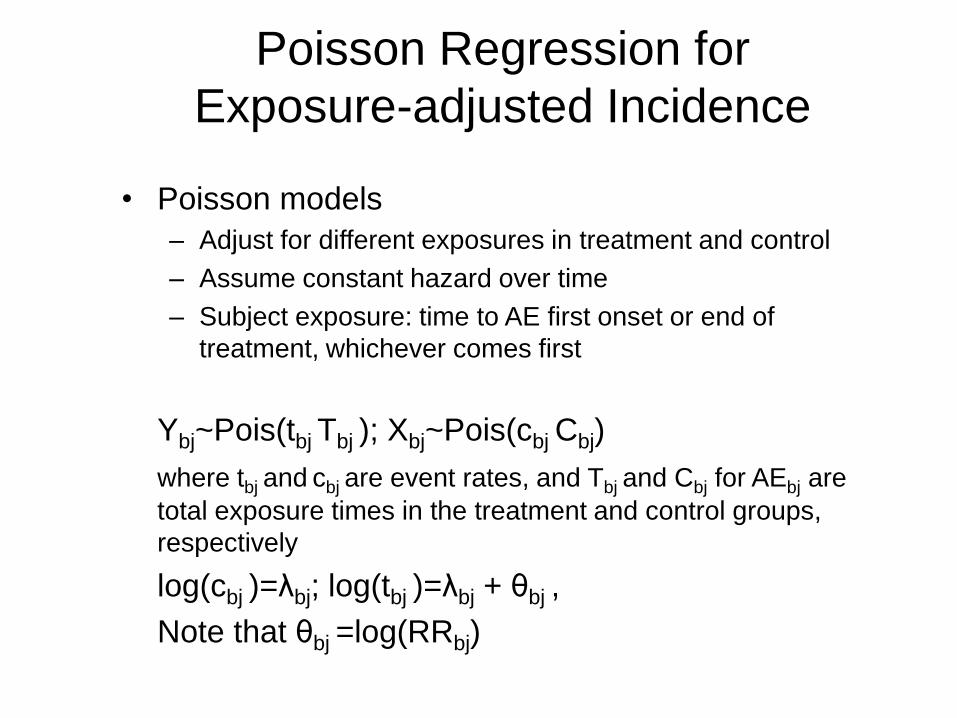
Poisson Regression for
Exposure-adjusted Incidence
• Poisson models
– Adjust for different exposures in treatment and control
– Assume constant hazard over time
– Subject exposure: time to AE first onset or end of
treatment, whichever comes first
Ybj~Pois(tbj Tbj ); Xbj~Pois(cbj Cbj)
where tbj and cbj are event rates, and Tbj and Cbj for AEbj are
total exposure times in the treatment and control groups,
respectively
log(cbj )=λbj; log(tbj )=λbj + θbj ,
Note that θbj =log(RRbj)
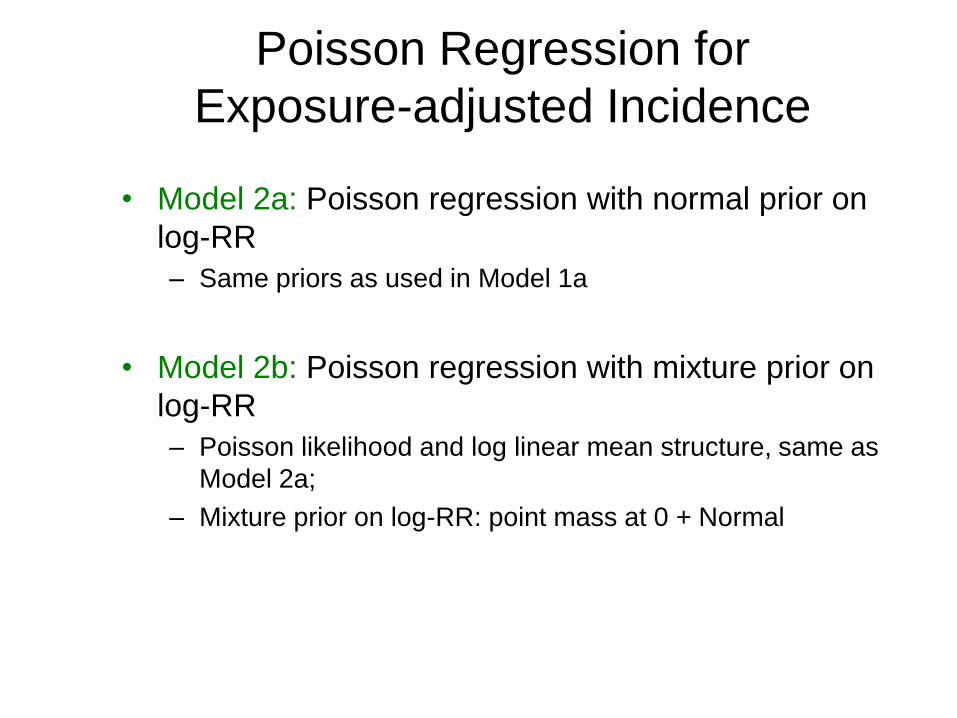
Poisson Regression for
Exposure-adjusted Incidence
• Model 2a: Poisson regression with normal prior on
log-RR
– Same priors as used in Model 1a
• Model 2b: Poisson regression with mixture prior on
log-RR
– Poisson likelihood and log linear mean structure, same as
Model 2a;
– Mixture prior on log-RR: point mass at 0 + Normal
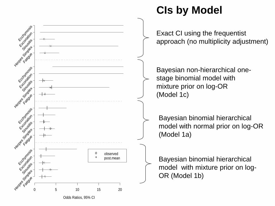
Exact CI using the frequentist
approach (no multiplicity adjustment)
Bayesian binomial hierarchical
model with normal prior on log-OR
(Model 1a)
Bayesian binomial hierarchical
model with mixture prior on log-
OR (Model 1b)
Bayesian non-hierarchical one-
stage binomial model with
mixture prior on log-OR
(Model 1c)
CIs by Model
Odds Ratios, 95% CI
0 5 10 15 20Fa
tigue
Her
pes Sim
plexS
inus
itis
Exc
oriatio
n
Ecc
hymos
is
Fatig
ue
Her
pes Sim
plexS
inus
itis
Exc
oriatio
n
Ecc
hymos
is
Fatig
ue
Her
pes Sim
plexS
inus
itis
Exc
oriatio
n
Ecc
hymos
is
Fatig
ue
Her
pes Sim
plexS
inus
itis
Exc
oriatio
n
Ecc
hymos
is
|
|
|
|
|
|
|
|
|
|
|
|
|
o observed+ post.mean
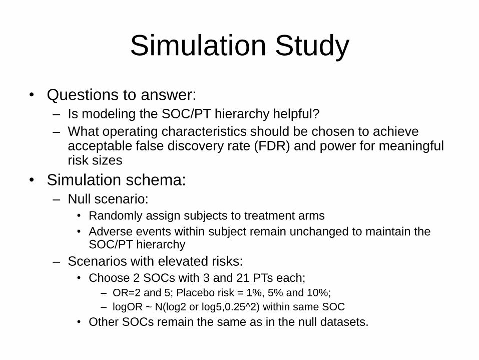
Simulation Study
• Questions to answer: – Is modeling the SOC/PT hierarchy helpful?
– What operating characteristics should be chosen to achieve acceptable false discovery rate (FDR) and power for meaningful risk sizes
• Simulation schema: – Null scenario:
• Randomly assign subjects to treatment arms
• Adverse events within subject remain unchanged to maintain the SOC/PT hierarchy
– Scenarios with elevated risks:
• Choose 2 SOCs with 3 and 21 PTs each;
– OR=2 and 5; Placebo risk = 1%, 5% and 10%;
– logOR ~ N(log2 or log5,0.25^2) within same SOC
• Other SOCs remain the same as in the null datasets.
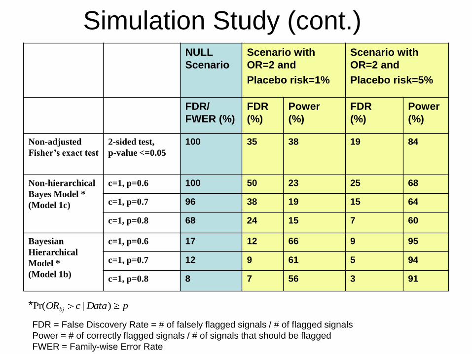
Simulation Study (cont.)
NULL
Scenario
Scenario with
OR=2 and
Placebo risk=1%
Scenario with
OR=2 and
Placebo risk=5%
FDR/
FWER (%)
FDR
(%)
Power
(%)
FDR
(%)
Power
(%)
Non-adjusted
Fisher’s exact test
2-sided test,
p-value <=0.05
100 35 38 19 84
Non-hierarchical
Bayes Model *
(Model 1c)
c=1, p=0.6 100 50 23 25 68
c=1, p=0.7 96 38 19 15 64
c=1, p=0.8 68 24 15 7 60
Bayesian
Hierarchical
Model *
(Model 1b)
c=1, p=0.6 17 12 66 9 95
c=1, p=0.7 12 9 61 5 94
c=1, p=0.8 8 7 56 3 91
pDatacORbj )|Pr(*
FDR = False Discovery Rate = # of falsely flagged signals / # of flagged signals
Power = # of correctly flagged signals / # of signals that should be flagged
FWER = Family-wise Error Rate
Closing Remarks • Current traditional approach of flagging
routinely collected AEs based on
unadjusted p-values or CIs can result in
excessive false positive signals – As a result, it can cause undue concern for
approval/labeling/post marketing commitment
• Bayesian hierarchical mixture modeling
provides a useful tool to address
multiplicity – Allows for explicitly modeling AEs with the existing
MedDRA coding structure so that AEs within a SOC
or across SOCs can borrow strength from each other
Closing Remarks (Cont.)
(Cont.)
– Appealing in the rare event setting
• The model modulates the extremes
• Inferences based on the „exact‟ full posterior distributions,
relaxing the assumption of normality of the outcome
– Models the entire AE dataset, so the distinction
between Tier 2 and Tier 3 AEs may not be necessary
• Makes efficient use of all the data
– Straightforward and flexible to assess clinically
important difference with different scales (risk
difference, OR, or RR)
• Avoid detecting medically unimportant signals (an AE could
have high Pr(OR or RR > 1 or RD > 0 | Data), but medically
unimportant)
Closing Remarks (Cont.) • Simulation study can guide selection of a
signal detection threshold
• Graphics are effective in displaying
flagged signals when analyzing hundreds
or thousands types of AEs
• The field of clinical trial signal detection is
still in its infancy – More research and practice are needed
– Further developments await statisticians work closely
with clinicians/safety scientists to advance this field

Thank You!
References • Bate A, Lindquist M, Edwards, IR, Olsson S, Orre R, Lansner A, and De Freitas
RM (1998). A Bayesian neural network method for adverse drug reaction signal detection. Eur J Clin Pharmacol 54:315-321
• Berry S and Berry D (2004) Accounting for multiplicities in assessing drug safety: a three-level hierarchical mixture model. Biometrics, 60: 418-426
• Chi G, Hung HMJ, and O’Neill R (2002). Some comments on “Adaptive Trials and Bayesian Statistics in Drug Development” by Don Berry. In Pharmaceutical Report, Vol 9, 1-11
• Crowe B, Xia A, Berlin, J, Watson D, Shi H, Lin S, Kuebler J, et al. (2009). Recommendations for Safety Planning, Data Collection, Evaluation and Reporting During Drug, Biologic and Vaccine Development: A Report of the PhRMA Safety Planning, Evaluation and Reporting Team (SPERT). To appear in Clinical Trials
• DuMouchel W (1999). Bayesian data mining in large frequency tables, with an application to the FDA Spontaneous Reporting System (with discussion). The American Statistician 53:177-202
• Gould AL. Drug safety evaluation in and after clinical trials. Deming Conference, Atlantic City, 3 December 2002
• Mehrotra, DV and Heyse, JF (2004). Multiplicity considerations in clinical safety analysis. Statistical Methods in Medical Research 13, 227-238
• O'Connell, M. (2006). Statistical graphics for the design and analysis of clinical development studies. Insightful Webcast: http://www.insightful.com/news_events/webcasts/2006/07clinical/default.asp
• Spiegelhalter DJ, Best NG, Carlin BP and van der Linde A (2002) Bayesian measures of model complexity and fit (with discussion). J. Roy. Statist. Soc. B. 64, 583-640.